dentification and lains and olling - twritwri.tamu.edu/reports/2013/tr451.pdf · groundwater...
TRANSCRIPT

Groundwater nitroGen source identification and remediation in the texas hiGh plains and rollinG plains reGions
Paul Delaune, Bridget R. Scanlon, Robert C. Reedy, Robert C. Schwartz, Louis Baumhardt, Lucas F. Gregory
Texas Water Resources Institute TR-451September 2013

GROUNDWATER NITROGEN SOURCE IDENTIFICATION AND REMEDIATION IN THE TEXAS HIGH PLAINS AND ROLLING
PLAINS REGIONS
FINAL REPORT
FUNDING PROVIDED BY THE TEXAS STATE SOIL AND WATER CONSERVATION BOARD THROUGH A CLEAN WATER ACT §319(H) NONPOINT SOURCE GRANT FROM THE U.S
ENVIRONMENTAL PROTECTION AGENCY
TSSWCB GRANT #09-03
PREPARED FOR: THE TEXAS STATE SOIL AND WATER CONSERVATION BOARD
AUTHORS: PAUL DELAUNE1, BRIDGET R. SCANLON2, ROBERT C. REEDY2, ROBERT C.
SCHWARTZ3, LOUIS BAUMHARDT3, LUCAS F. GREGORY4
1 TEXAS A&M AGRILIFE RESEARCH AND EXTENSION CENTER AT VERNON
2 BUREAU OF ECONOMIC GEOLOGY, JACKSON SCHOOL OF GEOSCIENCES, UNIVERSITY OF TEXAS AT AUSTIN, TEXAS
3 USDA AGRICULTURE RESEARCH SERVICE, CONSERVATION AND PRODUCTION RESEARCH LABORATORY
4 TEXAS WATER RESOURCES INSTITUTE
TEXAS WATER RESOURCES INSTITUTE TECHNICAL REPORT-451
SEPTEMBER 2013


i | P a g e
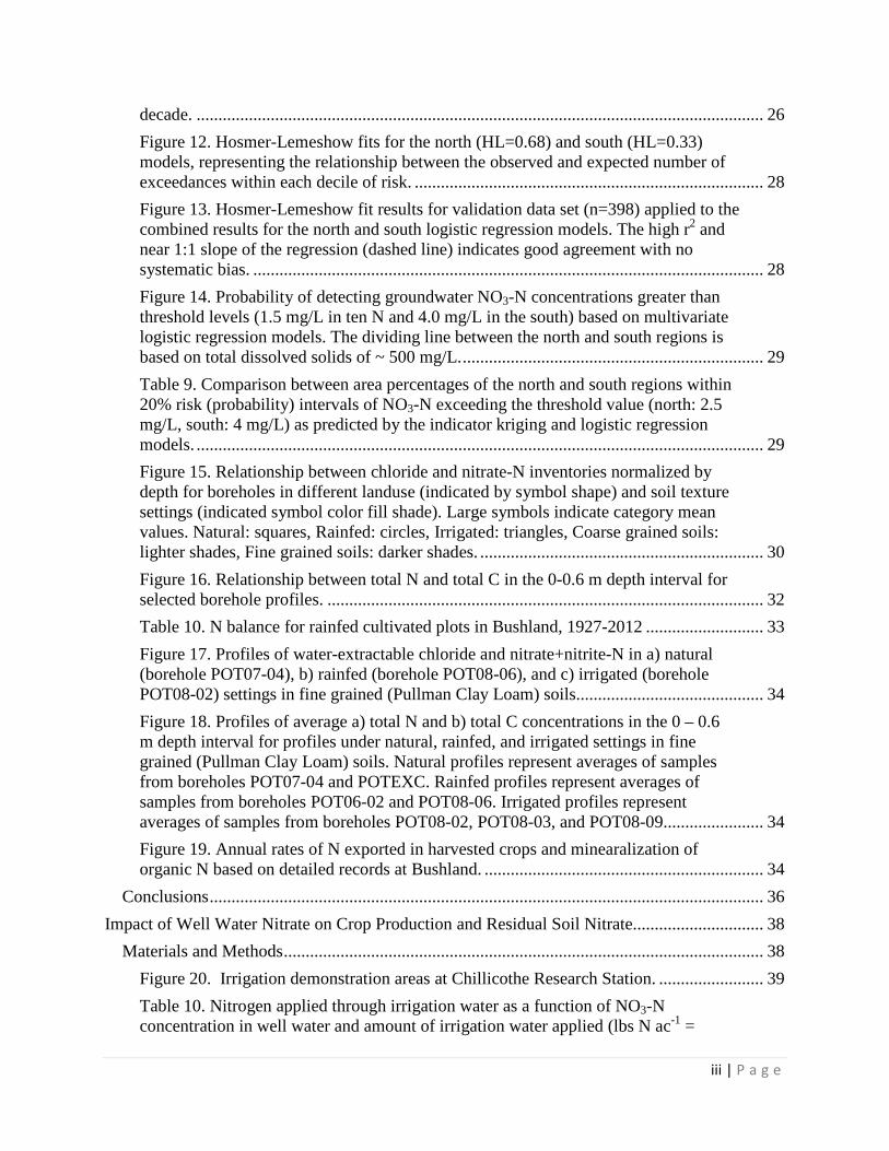
Table of Contents Table of Contents ............................................................................................................................. i List of Acronyms ........................................................................................................................... vi
Acknowledgements .................................................................................................................... vi Executive Summary ........................................................................................................................ 1
Introduction ..................................................................................................................................... 3
Figure 1. Distribution of NO3-N in groundwater in Texas (TWDB Data). ........................... 5
Figure 2. Concentration of nitrate and chloride in soil water in a 6-m soil profile in the SHP (Terry County) related to evapoconcentration. ............................................................... 5
Controls on and Sources of Groundwater Nitrate Contamination: Texas High Plains Case Study ............................................................................................................................................... 6
Study Area Description ............................................................................................................... 7
Figure 3. THP study area, land use, and borehole locations. Heavy black line depicts High Plains boundary in Texas and surrounding states. Land use percentages shown represent THP region values only. Irrigated crop area from Qi (2002) and remaining land use based on NLCD (2006). Irrigated crop area was calculated by subtraction from total NLCD crop area (38%), with remainder categorized as rainfed crops. ................. 8
Figure 4. Mean annual precipitation from PRISM 1981 – 2010 data (1 km resolution (www.prism.oregonstate.edu) ................................................................................................. 9
Figure 5. Mean soil clay content in the study area based on STATSGO (http://soildatamart.nrcs.usda.gov). Borehole locations and settings from Figure 3 are shown for reference................................................................................................................. 9
Materials and Methods ................................................................................................................ 9
Table 1. Total depths and inventories of Cl and NO3-N in boreholes completed in natural (rangeland) settings. Clay content and presence of Pullman soil series derived from SSURGO. ..................................................................................................................... 10
Table 2. Total depths and inventories of Cl and NO3-N in boreholes completed in rainfed (dryland) agricultural settings. Clay content and presence of Pullman soil series derived from SSURGO. .............................................................................................. 11
Table 3. Total depths and inventories of Cl and NO3-N in boreholes completed in irrigated agricultural settings. Clay content and presence of Pullman soil series derived from SSURGO. ........................................................................................................ 11
Table 4a. Rangeland setting borehole sample C and N analysis results. .............................. 13
Table 4b. Rainfed setting borehole sample C and N analysis results. .................................. 13
Table 4c. Irrigated setting borehole sample C and N analysis results. ................................. 14
Table 5a. Rangeland setting borehole sample N and C isotope analysis results. ................. 15
Table 5b. Rainfed setting borehole sample N and C isotope analysis results....................... 15
Table 5c. Irrigated setting borehole sample N and C isotope analysis results. ..................... 16

ii | P a g e
Data Analysis ............................................................................................................................ 17
Table 6. Univariate logistic regression analysis results, including standardized estimates and p-values of individual variables related to the probability of NO3-N exceeding 2.5 mg/L in the north region and 4 mg/L in the south region. Bold values indicate variables having p-values smaller than ~0.2. Larger standardized estimates tend to have smaller p-values. ............................................................................................... 20
Figure 6. Depth to water table in the High Plains Aquifer study area based on data from the TCEQ SWAP database. The THP is divided into north and south regions by the NW-SE trending line representing the 500 mg/L total dissolved solids (TDS) contour separating higher TDS concentrations to the south (median 874 mg/L, 751 wells) from lower TDS concentrations to the north (median 356 mg/L, 1,281 wells). The aquifer is traditionally divided into geographic regions defined as the CHP and SHP regions separated where the outcrop area is narrowest in the central Texas panhandle region. The 500 mg/L TDS subdivides the THP into a shallow water table zone in the south region (median depth 26 m) from a deeper water table zone in the north region (medial depth 62 m). ........................................................................................ 21
Results and Discussion ............................................................................................................. 22
Figure 7. Spatial distribution of NO3-N concentrations of groundwater sample analyses for 2,032 wells (points) sampled between 1988 and 2012 from the TWDB database. ................................................................................................................................ 23
Table 7. Pearson’s correlation coefficients (r) for relationships between NO3-N and groundwater major ion chemistry for different regions ........................................................ 23
Figure 8. Groundwater NO3-N distributions a) for all wells in the north and south regions and b) different well uses in the south region. Median NO3-N concentration in the south (4.8 mg/L) is 250% greater than in the north (1.9 mg/L). Within the south region, the median concentration for domestic wells (6.5 mg/L), which represent 30% of all wells in the south, is 150% greater than for all other well uses combined (4.4 mg/L)..................................................................................................................................... 24
Figure 9. LOWESS plots of groundwater nitrate-N concentrations versus well depth in the a) northern and b) southern regions of the study area. Vertical dashed lines represent the 10 mg/L NO3-N MCL and the 2.5 mg/L (a) and 4 mg/L (b) threshold concentrations used in indicator kriging. .............................................................................. 24
Figure 10. Spatial probability of groundwater NO3-N exceeding background concentrations of 4.0 mg/L in the south and 2.5 mg/L in the north regions of the study area based on indicator kriging of groundwater sample analyses for 2,032 wells (points) sampled between 1988 and 2012. Stable variogram models were fitted to the data with lag distances of 2.5 km (south) and 5.1 km (north), major range distances of 13.2 km (south) and 61.2 km (north), and anisotropy ratios of 1.2 (south) and 1.8 (north). ......................................................................................................... 26
Figure 11. Temporal trends in groundwater nitrate-N concentration distributions since 1960 in the a) north and b) south regions of the study area. Points represent the 50th, 75th, and 90th percentiles of concentration for samples pooled by decadal time intervals. Values at the tops of the graphs represent the numbers of samples in each
iii | P a g e
decade. .................................................................................................................................. 26
Figure 12. Hosmer-Lemeshow fits for the north (HL=0.68) and south (HL=0.33) models, representing the relationship between the observed and expected number of exceedances within each decile of risk. ................................................................................ 28
Figure 13. Hosmer-Lemeshow fit results for validation data set (n=398) applied to the combined results for the north and south logistic regression models. The high r2 and near 1:1 slope of the regression (dashed line) indicates good agreement with no systematic bias. ..................................................................................................................... 28
Figure 14. Probability of detecting groundwater NO3-N concentrations greater than threshold levels (1.5 mg/L in ten N and 4.0 mg/L in the south) based on multivariate logistic regression models. The dividing line between the north and south regions is based on total dissolved solids of ~ 500 mg/L. ..................................................................... 29
Table 9. Comparison between area percentages of the north and south regions within 20% risk (probability) intervals of NO3-N exceeding the threshold value (north: 2.5 mg/L, south: 4 mg/L) as predicted by the indicator kriging and logistic regression models. .................................................................................................................................. 29
Figure 15. Relationship between chloride and nitrate-N inventories normalized by depth for boreholes in different landuse (indicated by symbol shape) and soil texture settings (indicated symbol color fill shade). Large symbols indicate category mean values. Natural: squares, Rainfed: circles, Irrigated: triangles, Coarse grained soils: lighter shades, Fine grained soils: darker shades. ................................................................. 30
Figure 16. Relationship between total N and total C in the 0-0.6 m depth interval for selected borehole profiles. .................................................................................................... 32
Table 10. N balance for rainfed cultivated plots in Bushland, 1927-2012 ........................... 33
Figure 17. Profiles of water-extractable chloride and nitrate+nitrite-N in a) natural (borehole POT07-04), b) rainfed (borehole POT08-06), and c) irrigated (borehole POT08-02) settings in fine grained (Pullman Clay Loam) soils........................................... 34
Figure 18. Profiles of average a) total N and b) total C concentrations in the 0 – 0.6 m depth interval for profiles under natural, rainfed, and irrigated settings in fine grained (Pullman Clay Loam) soils. Natural profiles represent averages of samples from boreholes POT07-04 and POTEXC. Rainfed profiles represent averages of samples from boreholes POT06-02 and POT08-06. Irrigated profiles represent averages of samples from boreholes POT08-02, POT08-03, and POT08-09....................... 34
Figure 19. Annual rates of N exported in harvested crops and minearalization of organic N based on detailed records at Bushland. ................................................................ 34
Conclusions ............................................................................................................................... 36
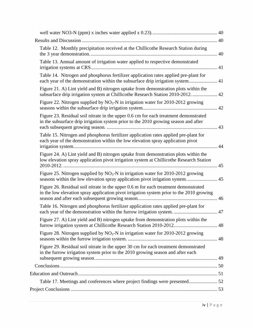
Impact of Well Water Nitrate on Crop Production and Residual Soil Nitrate.............................. 38
Materials and Methods .............................................................................................................. 38
Figure 20. Irrigation demonstration areas at Chillicothe Research Station. ........................ 39
Table 10. Nitrogen applied through irrigation water as a function of NO3-N concentration in well water and amount of irrigation water applied (lbs N ac-1 =
iv | P a g e
well water NO3-N (ppm) x inches water applied x 0.23). .................................................... 40
Results and Discussion ............................................................................................................. 40
Table 12. Monthly precipitation received at the Chillicothe Research Station during the 3 year demonstration. ...................................................................................................... 40
Table 13. Annual amount of irrigation water applied to respective demonstrated irrigation systems at CRS...................................................................................................... 41
Table 14. Nitrogen and phosphorus fertilizer application rates applied pre-plant for each year of the demonstration within the subsurface drip irrigation system. ...................... 41
Figure 21. A) Lint yield and B) nitrogen uptake from demonstration plots within the subsurface drip irrigation system at Chillicothe Research Station 2010-2012. .................... 42
Figure 22. Nitrogen supplied by NO3-N in irrigation water for 2010-2012 growing seasons within the subsurface drip irrigation system. ........................................................... 42
Figure 23. Residual soil nitrate in the upper 0.6 cm for each treatment demonstrated in the subsurface drip irrigation system prior to the 2010 growing season and after each subsequent growing season. ......................................................................................... 43
Table 15. Nitrogen and phosphorus fertilizer application rates applied pre-plant for each year of the demonstration within the low elevation spray application pivot irrigation system.................................................................................................................... 44
Figure 24. A) Lint yield and B) nitrogen uptake from demonstration plots within the low elevation spray application pivot irrigation system at Chillicothe Research Station 2010-2012. ............................................................................................................................ 45
Figure 25. Nitrogen supplied by NO3-N in irrigation water for 2010-2012 growing seasons within the low elevation spray application pivot irrigation system. ........................ 45
Figure 26. Residual soil nitrate in the upper 0.6 m for each treatment demonstrated in the low elevation spray application pivot irrigation system prior to the 2010 growing season and after each subsequent growing season. ............................................................... 46
Table 16. Nitrogen and phosphorus fertilizer application rates applied pre-plant for each year of the demonstration within the furrow irrigation system. ................................... 47
Figure 27. A) Lint yield and B) nitrogen uptake from demonstration plots within the furrow irrigation system at Chillicothe Research Station 2010-2012. .................................. 48
Figure 28. Nitrogen supplied by NO3-N in irrigation water for 2010-2012 growing seasons within the furrow irrigation system. ........................................................................ 48
Figure 29. Residual soil nitrate in the upper 30 cm for each treatment demonstrated in the furrow irrigation system prior to the 2010 growing season and after each subsequent growing season. .................................................................................................. 49
Conclusions ............................................................................................................................... 50
Education and Outreach ................................................................................................................ 51
Table 17. Meetings and conferences where project findings were presented ....................... 52
Project Conclusions ...................................................................................................................... 53

v | P a g e
References ..................................................................................................................................... 55
Appendix A: Cotton Nitrogen Fertilizer Calculator ..................................................................... 60
Appendix B: Education and Outreach Materials .......................................................................... 61
vi | P a g e
List of Acronyms CAFO confined animal feeding operation CHP central high plains CRS Chillicothe Research Station EPA US Environmental Protection Agency HL Hosmer-Lemeshow LESA low elevation spray application LLR likelihood ratios MCL maximum contaminant limit NANI net anthropogenic nitrogen inputs NLCD national landcover dataset SDI subsurface drip irrigation SHP southern high plains SOC soil organic carbon SOM soil organic matter SON soil organic nitrogen SSURGO soil survey geographic STATSGO state survey geographic SWAP Source Water Assessment and Protection TCEQ Texas Commission on Environmental Quality TDS total dissolved solids THP Texas high plains TSSWCB Texas State Soil and Water Conservation Board TWDB Texas Water Development Board TWRI Texas Water Resources Institute USDA ARS US Department of Agriculture – Agriculture Research Service USGS US Geological Survey Acknowledgements We are very grateful for financial support for this project provided by the Texas State Soil and Water Conservation Board and U.S. Environmental Protection Agency through the Clean Water Act, Section 319(h) Grant Program. We would also like to thank Dr. Thomas Boutton for analyses of C and N isotopes as well as local landowners for granting access to collect soil samples in the Texas High Plains.

1 | P a g e
Executive Summary Nitrogen in groundwater, more specifically nitrate, is common in certain areas and is often associated with agricultural production or urban areas underlain by coarse soils. While the presence of nitrates in groundwater is not debated, the specific sources or cause of the elevated nitrate in these areas is often questioned. The Texas High Plains and Rolling Plains regions are two areas in the state where elevated nitrates are readily found in groundwater and such questions regarding its cause and source are raised. These areas include portions of the Ogallala and Seymour Aquifers which both exhibit elevated nitrates in certain areas. The Ogallala Aquifer is the largest aquifer in the United States and underlies portions of eight states and 46 Texas counties. Consisting primarily of sand, gravel, clay and silt, the aquifer’s water generally meets established drinking water standards; however, isolated areas of naturally occurring and man-made pollution have been noted. Generally, its quality declines in the southern portion of the aquifer where total dissolved solids levels are elevated and naturally occurring pollutants are more common. Over 95% of the water pumped from the Ogallala Aquifer is used for irrigated agriculture but rural homeowners rely heavily on the aquifer for potable water. The Seymour Aquifer exists solely in Texas and underlies portions of 20 counties. An alluvial aquifer, the Seymour consists of gravels, sands and silty clays and is typically less than 100 ft thick. Water quality ranges from fresh to slightly saline in most areas with some very saline regions and elevated nitrate levels throughout its extent. Approximately 90% of water pumped from the Seymour Aquifer is used for irrigation while the remainder is used for human consumption. In an effort to address questions about sources and causes of elevated groundwater nitrate and to provide sound data on potential management strategies that can remediate groundwater nitrate levels, this project was developed. The primary objective was to identify sources of groundwater nitrate in the Texas High Plains and Rolling Plains and the secondary objective was to evaluate and demonstrate strategies and practices for reducing nitrate levels in these same areas. Collectively, this effort was able to provide insight into the potential sources of nitrate found in groundwater while also demonstrating how available nitrates can be captured as a beneficial resource and effectively removed from the underlying aquifer. Source identification efforts in the Texas High Plains and Rolling Plains indicated that the presence of elevated groundwater nitrates can be linked to physical features of the surrounding area as well as the uses of the land. Generally, nitrate levels increased in the Texas High Plains on a north to south gradient and are also associated with higher levels of total dissolved solids within the aquifer. As compared to the northern portion of this region, the south consists of coarser grained soils with lower amounts of clay and the average water table depth is also shallower. The probabilities of exceeding established background nitrate levels area were also calculated. In the southern portion of the area, the probability of exceedances is highest in areas where the water tables are shallow and irrigation is prevalent while in the north, the exceedance probability is highest where soils are coarser grained and nitrogen loads from fertilizer are higher.

2 | P a g e
Unsaturated soil profiles from various landuses were also evaluated to determine how nitrates migrate through the soil toward underlying aquifers. Findings indicated that under native rangeland conditions, nitrates are low while chlorides are high indicating that little recharge occurs below the root zone. Alternatively, in non-irrigated cropland, nitrate levels were found to be higher due to several factors. Soil organic nitrogen derived from organic matter incorporated into the soil profile when the prairie was first tilled was attributed as a considerable source of nitrates in deeper portions of the soil profile while inorganic fertilizer application was the primary source nearer the surface. Where irrigation is prevalent, nitrates in the profile are typically higher as are chlorides indicating that the application of irrigation water plus additions of inorganic fertilizers have contributed nitrate to the soil profile over the years. Once present in the soil profile and underlying aquifer, nitrate remains mobile and is readily transported in pumped irrigation water. As a result, it was hypothesized and supported by anecdotal evidence that irrigated crops would be able to utilize nitrates present in irrigation water similar to the way they utilize excess nitrate present in the root zone. To test this hypothesis, demonstration and control plots were established and planted to cotton under three irrigation scenarios in the Rolling Plains: flood, low elevation spray application pivot and subsurface drip. Results illustrated that lint yield was not adversely impacted by accounting for nitrate in irrigation water to meet the crops nutrient requirements. Additionally, substantial cost savings can be realized by the producer applying this technique while effectively ‘mining nitrate’ from the aquifer below. If this practice of ‘nitrogen crediting’ is implemented on a broad enough scale, it could reduce nitrate levels in the aquifer over time and ultimately improve groundwater quality. Incorporating soil sampling to at least 30 cm, and preferably 60 cm will further improve nitrogen harvesting abilities by accounting for residual nitrogen stored in the soil profile and will minimize the potential to leach nitrogen through the soil profile and into underlying aquifers.

3 | P a g e
Introduction Groundwater nitrate contamination is widespread in the US, mostly in agricultural areas in the High Plains, Midwest, Central Valley of California, and other regions (Nolan et al., 2002, 2006). High nitrate concentrations in groundwater can have adverse health impacts and as a result, the federal safe drinking water standard, or maximum contaminant limit (MCL) has been established at 10 mg/L NO3-N. Above this level, the risk of adverse health impacts increases. Conditions commonly associated with continued consumption of high nitrates in groundwater include methemoglobinemia in infants which is a potentially fatal disease resulting from low oxygen levels in the blood (Spalding and Exner, 1993). An increased risk of developing non-Hodgkin’s lymphoma has also been related to nitrate concentrations ≥4 mg/L nitrate in community water supply wells in Nebraska (Ward et al., 1996). Toxicological studies indicate that multi-contaminant exposure such as nitrates and pesticides, may have a much greater impact on health than exposure to single pure contaminants because of additive or synergistic interactions among compounds (Squillace et al., 2002; Porter et al., 1999) and suggest that the MCL for nitrate should be reduced. If implemented, this would affect water availability in Texas. However, other studies suggest that the basis for the MCL of 10 mg/L NO3-N should be revisited and possibly raised (Powlson et al., 2008). The Seymour Aquifer is a shallow aquifer underlying over 300,000 acres in 20 counties in northwest central Texas. According to Table D.1 of the Texas NPS Management Program, the Seymour Aquifer has the highest aquifer vulnerability rating of all the major aquifers in Texas. This indicates the aquifer’s high susceptibility to impacts from surface activities. High nitrate concentrations are widespread in the Seymour Aquifer. In their 2008 Texas Water Quality Inventory Groundwater Assessment, the Texas Commission on Environmental Quality (TCEQ) reported that ambient groundwater quality data collected from 1999-2006 shows that of the 91 wells sampled, 83 exceeded the nitrate maximum contaminant limit (MCL) of 10 mg/L. All 91 wells had detectable levels of nitrate. Median nitrate levels in Knox, Haskell, Baylor, Hall, Wichita, Wilbarger, and Fisher counties exceeded the federal safe drinking water standard (10 mg/L NO3-N), with some exceeding 40 mg/L. Additionally, this report indicates that 15 sites had confirmed groundwater contamination with atrazine, dicamba, prometon, and propazine due to nonpoint sources (TCEQ, 2008). A study by the University of Texas Bureau of Economic Geology found that nitrate accumulations beneath irrigated agriculture are generally high. High levels of nitrate in groundwater prior to fertilization and irrigation in the Seymour aquifer, low to moderate fertilizer application rates, and low to moderate unsaturated zone nitrate accumulations indicate that high groundwater contamination may be related to natural nitrate sources prior to irrigation and to irrigation recycling. These high concentrations are a concern because although 90% of the water from the aquifer is used for irrigation, it is used as a municipal water source for Vernon, Burkburnett, and Electra and rural families in the region. In addition to the use of groundwater from the Seymour Aquifer for irrigation and municipal purposes, the aquifer also naturally discharges through seeps and springs. This natural discharge contributes to the baseflow of many streams throughout the region. Groundwater flows toward the east-southeast, heading to the perimeter of the Seymour deposits. Stream flow increases towards the perimeter because stream stage is at a lower elevation than groundwater in the

4 | P a g e
Seymour aquifer. Nitrate is a concern in a number of waterbodies in the region including Buck Creek, South Groesbeck Creek, Wichita River Below Diversion Lake Dam, and Paradise Creek. Activities designed to reduce nitrate levels in the aquifer may also benefit area streams receiving baseflow from the Seymour Aquifer. Currently, producers do not account for the high nitrate levels in the irrigation water they apply from the Seymour Aquifer. Underutilization of water testing, historical low cost of fertilizer, and speculation regarding the amounts of nitrate in the irrigation water that is actually available to crops prevent widespread accounting of this nitrate source. As a result, this lack of crediting has in many cases led to over-application and build-up of soil nitrate which increases the potential for N transport to surface and groundwater water supplies. With the recent increases in fuel and fertilizer costs, farmers are searching for ways to better manage their nutrients and make their operations more efficient and profitable. Thus, the stage is set for positive changes in nutrient management. In the Seymour Aquifer Water Quality Improvement Project Final Report (Sij et al., 2008), it was recommended that educational programs on irrigation management and nutrient management be provided to encourage regular soil testing, better manage irrigation systems, and account for nitrate levels in irrigation water when determining N fertilization needs. The report suggested that if nitrate in the aquifer could be “mined” using irrigation, then substantial cost savings could be realized by producers as a result of reduced nitrogen fertilization. It is estimated that irrigation water from some wells could supply the entire N requirement of a cotton crop (Sij et al., 2008). This in turn could potentially improve the quality of the water in the aquifer and streams receiving water from aquifer. Groundwater nitrate contamination is also very important in the Texas High Plains (THP) and the Ogallala Aquifer. Groundwater contamination is most widespread in the southern half of the Southern High Plains (SHP) where 25% of all wells exceed the MCL of 10 mg/L nitrate-N (Scanlon et al., 2008). Understanding the source of nitrate in the aquifers is essential for mitigating the problem. There are a variety of potential sources of high groundwater nitrate concentrations in the THP (Ogallala) and Rolling Plains (Seymour) Aquifers. High nitrate concentrations are generally attributed to a surface source because of high correlations with water table depth and negative correlation with aquifer saturated thickness as a result of reduced assimilative capacity. Potential sources of nitrate in groundwater include atmospheric deposition, natural sources, inorganic fertilizer, organic fertilizer (manure), concentrated animal feeding operations (CAFOs), barnyards, septic tanks, and leaking sewer systems.

5 | P a g e
Figure 1. Distribution of NO3-N in groundwater in Texas (TWDB Data).
Figure 2. Concentration of nitrate and chloride in soil water in a 6-m soil profile in the SHP (Terry County) related to evapoconcentration.
In the High Plains and Rolling Plains, the most widespread source of nitrate is from fertilizer application. However, preliminary results from a recent study suggest that much of the nitrate in the SHP could be natural, originating from mineralization of soil organic matter (SOM) associated with initial soil cultivation (Scanlon et al., 2008). These data include high nitrate concentrations that extend into zones of high chloride concentrations in the unsaturated zone, indicating old soil water that pre-dated cultivation. The mechanism for release of nitrate from SOM is attributed to increased aeration and increased moisture content associated with cultivation and is shown by soil moisture data. Nitrogen isotope data from soil water could not be used to distinguish natural sources from fertilizer sources because fertilizer nitrogen is derived primarily from ammonium-based fertilizers that undergo similar processes to natural mineralization of SOM. If the nitrate pulse is related primarily to natural sources, then this source should eventually move through the system as a pulse and groundwater quality should improve with time. Reservoirs of Nitrate in the Soil It is difficult for farmers to determine if they are over applying nitrogen to their fields without knowing the nitrogen content of their soils and water. Drilling and sampling soil profiles provides excellent information on long-term nitrogen transport in the subsurface. Preliminary results from drilling in areas of different land management indicate that the largest nitrate-N reservoirs are restricted to irrigated agriculture with maximum concentrations ranging from 93 to 430 mg/L (Figure 2). Large bulges of nitrate are accumulating under irrigated settings because of over application and inappropriate timing of application (50% applied pre-plant). Educational materials need to be developed for agricultural and water resource managers to show that nitrate is currently being over-applied and is being leached below the root zone, particularly in irrigated areas. With increasing costs of fertilizers, such information would be extremely valuable to producers and could result in large scale reductions of nitrogen fertilizer applications.
#
##
#
#
##
### #
######################## #
###
#
###
### #####
##
###
#
##
###
#
##
#
#
###
# #
##### ############################### #### #
##
# ## ## ### ##
################ #### ## ### #
########################################
##
#
######## # #
######
#
#
##
#
####
###########
##
#
#
#
#
#
###
##
####
#
#
######
#
#
#
#
##
#
### #
###
#
#
# #
#
##
# ### ###
#### #######
### ### ###
# ### ##
########
#########
# ##
#
## ## ###
#
#
### #
#
###### #
# ############
##
#
##
##
## #
##
### # ## ## #
# #
### ## #
# ##
# ##
# # #
## ### ## ## ### # ## #
# # ##
##
# ## ###
#
#
# ##
##
#
#######
## ## ##
##
##
#
#
#
#
# ### ###
#
#
###
# #
#
#
####
#
###
#
##
##
# ##
#
#
## ####
## ###
########### # #
### #
##### #
###
##
# ## # ## # ##### # #
### ##### ## ##### # # #
# # ## ## ## #
## ## ## # ### #
### # ##### #########
###
######## ########### ###### ##### ######## # ###
###########
##
##
# ################# ##### ################
#### ##### ## #
## #
## ## #
##
## #
# # ####
#
####
## ###
## ## ### ## ## ### ## # ####
#
# ##### ### ## ### # ## #### ## ## # # #
##
### ## ##
#
#####
###### #
# ## ### #### #### #### #
## ## #
### ### ##### #######
#
# ### ## ##
###
###
## ###
#
# ###### ##
### #
#
# ###
#
#
## ##### ##
# # ##
# #
#
##
## ###### #
#### ### #
##
#### #
##
# ###
#
##
##
#
#
## ##### ## ###### ### #### #
## # # ###
#
#
# # # ###
## #
###### ## #
## ## #
#
###### # ##
### ####### # ##### ######## # #
## #### ### #
#
####
#
#
###
### # ###
# #
## #
#
#
##
#
#
#
## ## # ##
#
#
# #### #
# ###### #
#
## ## #
##
# #
#
## # # #
# ## ## ###### #
#
# # # ## ##
# # # #### # ##
#
#
#
#
###
#
####
#
#
# #
####
####### ###
###### ###
#
#
#
# #####
#
#
#
###
##
# ##
#
#
#
#
##
## #
#
##
# #
#
###
#
#
# #
##
#
### # # #
# # # ### # # ##
# ## #
# ## # #
## ### ## #
# # ## #
## #
# # # ## ## #
# ###
# ##
# ### ### #
##
#
####
#
##
####
# ## #
#
# ## ##### ####
##
#
### #
## ## ## # # ### #
# ## # #
#
# # ### # # #### # ###
# ###
## ## #
#
# ### ## # #
#
#
#
#
######
##
# ###
# #
### #
# # # ###
## # ## #
###
# # ### ### ## ###
### #
#
# # # ###
## ### ## # # #
# ##
## #
### ####
#
## ## #### # ##
###
##
# # ## # # ## ##
# #### ### # # ###### ####
# # ## #
## ### # #
# # ### # # # ## # ## # ##
## #
#
## # #
#### #
#
# ### ## # #
#####
### ##
### # #
### # ##### ###
#
# ### #
# ### ##
# ###
# #####
# #### # ## ####
# #### ## # # #####
####
# ## ## ######
##### # #### ## # # ###
###### # ### #
## # #
# # ### #####
# # ## ## ## # # ####
###
### ## ## ###
###
## #
#
####
#
# #
### #
## #
# #### ###### ###
# ##
##
#### ########
################
# #
#
#
### #
##### ## ##
#
###
########
##
### #
#
## ######### #
#### # #
### ### #### #
#
## ##
## #### # #
###
#### ### ##### #
### ##
###
##
## ### # ###
## #
### #####
# ####
##
#
########
##
#
######
# # ###
##
#
##
###
###
######
## ## ###
##
#
#
#### #
# ##
#
## ### ##########
###
##
###
#
#
#
### #
#
## ##
### ### ### #
#
####
##
## ###
#######
##
#
#
#
##
#
# #
###
#### ##
######
### #
#### #####
####
#
###
#
#
#####
#
##
# ##
#
######
##
# ### ####
# ## ###
##### # ##
# ##
### ## #########
#
########
####
###
#### ## # ##
#####
#####
###
## #
#
# #
##
###
##
#
## ##
###
#####
##
#
#### ##### ##
## ##
#
##
# ### ##
### #
##########
#
########
###
#
# # ###
#
##
#
###
############
######## #
# ## # ##### # #
# # ####
##
# ##### #
## # ##
# ### #
#####
## ####
###
#######
##### #
#
# ## ## #
##
#
####
### #####
#
##
## #
# #####
# ################
###############################
#
### ####
#
##
## #####
###
#
#
##### ##
###
#
#####
###
####
##
##########
#
# #### ############# ####
######
######
#
##
#
################# ########################
################################
#########
##
##
# ##
# ## #### ##### # #
# # # #
##
## ##
#####
#
## #
##
## #####
#######
##
###
#
#
####
######
#
##########################################
#######
#
#
##
###
#
##
#
#####
#
###
#####
#####
###
####
### # ###### # #
###
#### # #########
##
##
### ## ## #### ## ### #
########
## #########
##############
############## ####
######
###################################### #
# #######
##
##
#
####
# ## # ###
#####
#####
###
######### ###
#
##
#
### # #
#
######
### ##
### ##### #
# ####
#####################
####
####### # ################ #####
#####
########
#######
######
# ## #### # ###
### ##
##
#
####
#
##
#
#
#
#
#
#
#
#
##
#
##
#
#
#
#
## ### ## #
#
#
#
# ### #####
#
#
#
## #
########
# # ###
#
# ##
###
####
##
#
##
#
## #####
# # ## ##
# ##### ### #
##### ##### ## ##
# # #### #
# ## #### ### # ### ## ## #####
### ########### ### #### ##
## ##
###### #
##
## # ###
###
### # #######
##### #
## # # ## #
#
## #
##
# # ## #
### ##
# #
### ### # #
# #### #
# # ### #
# #
#
## # #
# ## # ###
## #
#
## ###
#
###
# #####
####
###
#
## ###
##### ##
################## ############# ######### ################# #
### # #
############### ###############
###
## #### #
#############
## #
# #####
## #
#
##########################
###
# ##
# ## ##
# ##
##
##################
#
# #
#
## # #
### ##
#
#
# ################# #### ### ###### #
#
## ###### #######
#### #
## ##
# # ## ####
##### # ## #
# # ## #
## #
## ## # ##### ### # ## # #
#
## #
# ### ##
####
# #
## #
# # ### # ###
#
### ### #
# # ## ##
## ##
#### #
##
# #
##
##
###### # ###
## ###### #
## #
##
### #### #
## ##### ##
#
#
##
# #
# ###
#
#
#
##
###
# # ###### ### ###
# #
##
##
# #####
###
## #
##### #
#### ## #
## # #
#### # ##
#### #
##
## # ##
#####
# #
### ### # # ### # #
#### #
##### # ## # ##
# # ## ## #### ### # ### ##
# ## ### ## ## ##
# ##
# # ## # ## # ## ## ## # # ## #
# ##### ####### ##
# # #
# #
#
## #
#
# ###
#
##### ############ ##### ### ########## ### ##### ## # ## ##### ###### #
# ######## ##############
#######
#
# #
##
# ###
## # ## # #
# ## #
## ## # #
#### # #
### ## # ##
## # ##
## ##
# # ##### # #
# ## ## ##
#### # #
# # ## # #
#
#
# ###
# ##
###
##
# #
##
###
# # ## #
##
#### ###
##
#
#
##
#
# ##
#
# #
#
### #
# # #
#
# ### # #
#
#### ##
######
##
#
#
##
##
#
########### ### #
# ## ## ###
##
#
########
#
#######
###
##
# ###
#
#
##### #
#
### #
#
#
#### ##
#
### ##
##
#
# #
#
### #### # # #
#
###
## #
#### ##
#
##
##
# #####
###
## #
# ### #
#
# ## #
# # ####
## ######
# ## ##
# # #
##
### # #
### # # # ######## ####
# ## # ### #
###
##
#
# #####
#
#
# #
#
##
#
###
##
###
#
#
##
#
##
#
#
#
#
##### # #
#####
## # ##
# ###
##### #
##
#
#
# ######## #
# #
# ## ### ##### ## ###
##
# ##### ##
### ##
###### #
##
#
#
#
#
#
#
#
#
#
#
## #
##
###
#####
##### ## ### #
# ########
# ##### # ##
# # # ## #### ######
##
## #####
# ## #####
#
# ## ## ####### #
# # # # #### #### ## #
# ######## ### # #
### # #### # #
### ## # ### ##
#####
#
##
### #
#
########
###
# #
###
## ### #### ## #
# #### # #
# ## # #
#
#
#
#
#
# # #
# # ##
### # ## ## ## # ###
## ### ### ##
# ####
## ## ###
# ####
######### #
### ### ##
## #
## #
#
###
# # ## ##
# ###
#### ## ### ## #### ### #### #
# ## # #### #
#
## #
######
##
##
##
##### ##
## ###
#
#
# #
###
# ##
#
#
#
#######
## ##
###
##
#
#
###
# ##
# #
#
#
# #
#
####
# ##
##
###
#
#
# #
##
##
### ###
#
##
## #
#### #
### ##
###
### ## ####
#
#
#
###
#
# #
#
#
#
#
# ##
####
# #
#
# ###
# ####
##
########### # ####
### ##
##
#
##
# ###
#
#
##
###
########## #
# ##
#
#
#
## ## # #
## ##
##
#### #### # # ## #
#
####### #
# ###
##
###
#
##
# ## ## ## ## #
### # #
## #
# #### #
## #
##
##
###
##
# # ## # #
## # # #
# # # ## ##
##
## # ##
# # # ###
# ## ## # #
# # ###
#
# ###
##
# ### #
# ## ## # #
## # #
# ### ## ### # # #
### # ## #
# # ###
# # ##
### ####
##
# ## ## ##
####### ## ## #
# # ##
## ## ##
# ### ###
# ####
##
####
###
##
#
# #
#
## #
#
###
#
## #
# ##### # #
#
##
#
#
#
#####
# # ##
# #
## #
##
## ## # ##
# #
#
#
## ## ## #
#####
# ###
#
######
## #
#
#
# # # ## #
# ### ### ######## ##
## ## # # #
### ##
## ## ###
# ######
#
# ## ## ## ## #
# # ##
###
##
##
##
####
# #
##
### # #
##
#### #
# # # # ## #
## # #
##
## # # ###
## # # #
# # ##
##### ## ## # ##
# # ## #
#
# ## #
## ##
#
#
# ## #
#
# # # #### ##
# ### # # #
# # ## #### #
## #
## ## ### #
# ## ### ##
###
## ##
##
## ##
#
##
## #
# # ###
## #### ##
## ##### ## # #
# ## # ### # ###### ###### #
# # #
###
# ## # ##
# ###
##
####### ##### # ### #### ####### ##
#
#
#######
#### #
#
#####
# ## # # #
# # ## # #
### ##
## # ### ## # #
## ## # # ### ## # # ##
## #### ##
### # ## ##
### #### ##
## ## ##
# ###
## # # # # #
#### # #
### ## ## # #### # # ## #
##
# ### #
# ## ### ## ## ## # #
## ##
# # ####
# ## ### #
## ### ### # # #
# ###
## ##
#
##
# ##### ## ##
# ########
##### #
# # ###### # ##### # #
# ### ## ####
###
## #### ##
# # ## # #
# ######
# ## # ####
# ### ####
# ## ## # ### ## ## ## ## ## # ## ## #
# # # ######### #
# ## # ##### #
# ## ###### # # ## ## #
######
### # ## #
#
#
## #####
##
# ##
#### # ###
## # # # ##
# # ## ##### # #
# #
# # ##
# ## # ##### ### # # #
# ### # # ###
### # ##### # ## ##
# # # ## #
# ## #
#
# ## # ### # ##
#
###
##
## ##
### ## #
###
# ###### ## ### #
### #### #### ####
# #######
## ## ##### ## ### #
# ### ### # # ### # ##### ## # ###
###### ##
# ## # #
##
##
######
##
######
#
### ##
### #
#
#
##
# ##
# #### # #
# ## ##
## # #
# ####### #######
#### #
###### #
######################################
################
## #########
########### # ##
#######
#
##
## #
##
# ##
##
# ### ###
#
#
#
# #
#
### ### #
##### ##### ##
# ###
##
# ## ### ##
#
# ##### ####
#### ######### #####
#
#### #### #### ############
#
#### ### ###
## ###
## ###
#
#
# #### ######
#
#### ### ###
#
#### #### ###########
#####
#### ######### ##
#
### ########
#
#
#########################
######## ###
# ############
###### ##
# ###### ### ##
######### ############ #####
##
# ########################### ###
##
################## ##################################
###################### ################
######
#
# #
###
###
#########
#
#
#### ###
##
###
##
#
# ##### ### #######
#
##
######
#
#####
# #
###
#######
#
######
################ ######## #
# ################
# ####### ###
#### ###### ##### # ##
####
##### ####
#
#
#
## # ## ## #
# ####
#
#
#
#### # # ### ######## #######
###
########### ######
########
#######
##
#
#
# ###########################
##########
#
###
####
#
#
#
# # #
##
#
# ## ## #
##
######
##
#
#
###### #
### # # #
# ################
# #### # ## #### ###########
##
# ##### ####
##
##
# ### #
### ################## #####
# #### # # #####
#
#
## # ##### ####
## ### #
##### # ## ######## #
### ##
### ####### ######### #### ########## ####
####
## # # ##
# ##### #
### #
## ## # ### ### #
# ## ## ## ###
## #################### ##### ############### ##
## ### ####### # ## # #### ### ### # #### ## ##### ### ####
# ## #### # ###
## ## #
##
#
#
##
##### ######
# ## ### ####
#
## ##
#
##
######
## ##
##### # ### ### # ### ## ######## #### ######### #######
#### #####
# ######
##
## ## #
####### ### ###########
# ### ## # #
##### ###### # # # #
#
#
##########
### # ## ## ## ### ## # ####
# #
### # #### ### ######### ##### #
### #### ###
################ # ######
###
#
##
##### #
# # ### #
############################
#
###
##
#
#
#
#################
#
#######
#
## #### ##############
######
#
#
#
#
#
######### ###
#
#
##
#
#
# #
#
#
####
#
## #
####
### #
# # # #### ##
# ###
# ######### ## #### ##
# ##
############################ # ####
# ####
## #
# ## ######## # ##
## #### # ####### ###
# ## #
#########
# ######## # ############
# ## ########
##
# ###### ### #
##### ##
# ############
##
# ##
### # ###### # ##
###
##
##### ########################## ##
#### #### ####
# ## ###### ###### #
####
### ### ###### #
##### #### ###
############ ### ####### ##### ####### ## ##
## ####
# # ######## ### ## ############### # ##
###################
###########
###
# # #
## ##### # #
# ### ##
# # ###### # ###
# ###
## #### #
# # ### # #
# ###################################### #
# #
##### #
### ####### #
# ### ## #
######
##
# ##############################
#
#
#
####
##
##
##
#
###
#
##
#### ##### #
### # #
## # #
#
## # ### # # ### ###### #
# ##
###
# ## # ###
# # ### #
######## ## # #
## # ## #
##
#### ## ## # ## ### # ##
######### ### # # ##
##### # ####
#
## # ## ## # # # ### ##### # # ###### #
#
## # #### ### ##########
############### ## #################
##
## ###
# ## #### # ## # # # #### ### ## ## ###
# ## ## # #
# # # ### ## ##
#### #
# ####
## ## ## # # ### # #
## ##
#
# #### ### ## ## # ###### #
# ## ## # ######
###
# # # #### # # #
#
# ### #
#
############################
## ##
# ###
## # # #
# ####
## #
#
####
# #
##
## ### #
## # # ### # #
## #
#
## #
#
#
##
# # ####
#
## # #
#
###
#
# ### #
##
#
#
# ## #
#
##
##
# # #
## # ### # # ####
### ## # ## # #
# # # # ##
# ## ## ## ##
# ## # ## ##
#
## # #
# ##
###
## # ### # #
# ### ## ### ### #### ## ###
### #
# ## ##
## ##
## #
## ##
#
#### ## #
# #
# #
#
##### ### ##
#####
### ####### #
# # ###
#
####
###
## #
##
# # ### #
##
# #
# ###### ## #
# #
###### #### ########### #############################
#
########### ########
# ####
############################
## ## # # ##### ### # # # ########## # # ### ###
# ## ## ## # ## #
# # ## ## # ###
# #######
# # ###
## ## ##### #
## # ## ##### ###### ## ## ### # ## #### #
##
#
## #### # #
# # ##
### ### # ## ### ### # ### ### #### ##
# # #### # # ###### ##
# # ## # ### ### ### #### ## ###### ## #### ##### ## ## #
# #
## ## ####### # ## ## #
## ##### #
##
# #
#
##
# # ## # ##### ##
# # ###
### # # ###
# ### ## ## ##
####### ##
##
##### #
# #### #
# ## # ## ##
# ###
## # ## ## ### # #
## ####
#### # # ## ## ## ##
#####
# ## ### # ## ### ## ### #### # #### ## ### # #### ### ###
#
#
##
###### #### # #
# ### # #
### ## #### ##
### # #########
### #
######
## ###
## ##
#
###
####
## ###
### ## # # #
###
# ##
#### #######
###### # ####
## #
## # #### ###### ###
###### ######### # ### ###
## # #
########
### ##### # ######## ####
######### #######
# ########
######## ## ########### ############# ## # #### ### ###
##
#### # ###### ## #### # ## ### ## ####### ###
###### ### # # ### # #### # ##### ######
# ## # ## ####
# ### ## ## ## ##
# ## ### ###### # ## # ###
## # # ### # # ##
#### ##
###### ## ## ##### ####### #
##
####
# # #### ## #### ### ##### ########
## #### ###### ## #
#### ###
### ## ### ####### ################### ## ##
### ##### ## # ### # # ### ####
## # # # ### #####
#### #### ### #####
## # # #####################
#####
#
## ###### ##
## ###### ## ## #
##### ## ## ########## ############# #
# ## ###
## ##### ############ ## ######### ## ##### ## ### # ########## #
# # ###### ## ########## #
# # ## ########### #
############
###### ## ########## ######
#### ## # # # # ## ###### ###### #
# # ### ## ##
## #### ####
####### ## #####
##### # #### ### ## ### # #### #
############################################################################################
####
##
### #
#
#
##
######
### #
### ### #
## #
##
##### #
#####
#
#
#
# #### #
##
#### ## ###
#
#
#
##
# ### # # #
##
##
#
#
#
## ##
######
#
#
##
#
#
###
#
#
# ### ###
## #
###
### ##
## # #
## ### #
# # #
####
############
# # ###
### #### ##
######## # ### ###########################
# ## ##############
################### #########
########### # ##########
##
#######
#
# ##
## ##### #######
# ###
# # ### ## ## #
# ###
#
# #######
# ##### #
# # ##
# ## #
####
### ##
## # # #
# # ###
#
#
#
# ### #
# ###
### # ## ##
##
#######
####
#
#
#
#
##
#
##
##############
### #### ##
# ## ###############
########## ####### ##
##
# ######
##
#### ### #
# #
#
###
###
#
#
#
#
#
###
#####################
## #####
##
#
#
###
###
##
# #
#
#
#
#
#
#
###
#
###
#
# #
# ### #
### #
## # ##
#### ##
##
#
#
##
#
#
##### ###
##
# ##
# # ###
## ##
###### ##########
#
##
#####
###
##
##
########### ##
#
###
#
# ###
#
#
# ###
#
#
##
## #
#
# ##
##
#
# ### #### #
######
# ##
##
###
###
#
#
##
##
###
#
###
# #
##
#
#
#
########
###
# ### ##### ## #
###
#
## ## #
#
##
#
## ##
####
#########################
##
# #
#
### #
########
#
####
# ##
#
#
##
###
# ####
## ##
######
# ##
# ### ##
# #
#####
#
#
#
#####
##
##
#
#
# ### #
##
##
# #########
## ### #
#### ### ##### ####
## # ########
#### ## ## ##############
##### # ##
### ### #
### ##
# #
###
##### ###
# ###### # #
### ##
# #### ##### ####### ####
####
# ###
#
#
####
####### ##### #
## #
##
##
#
#######################
################################### #
#
##
#
#
#
#
##
##
######
########
# ####
### #
## ## ##
#
#
##
#
#
##
#
##
#
#
#
#
##
####
#
# ## #
###
##
### #####
# ##### ###
#
#### #
#
#
### ##### #
#
#
###
###
#
#######
#
##
#
#
#######
# #
#
##
#
#
# ##
#
#
#
#
#
#####
## #
#
#
# ### #
#
### #
#
######
#
#
##
#
## #
#####
# #
## ##
###
###
#
##
#
# #
#
#
#######
#
#
#
#
####
#### ###
#
#
#
#
#
#
#
##
#
###
# # # ### # ### # # #
#
#######
#### #
##
### ##
##
#
#
#
#
##
##
#
##### ##
##
###
####
#
##
##
#
#
#
# ##
# #
#
#
# #
#### #
# #
# ##
###
#
##
#
#
### ##
##
# #
#
##
#
##
## #
##
#
####
##
## #
#
#
# ###
## #
#
# # ##
## ##
##
#
#
###
#
#
##
##
#
#
# # ###
# #
#
#
# ## #
#### #
##
# ## ### #
#
##
#
# ##
#
# #
### ### #
##
#
##
# ##
# #
#
##
# ##
####
##
### # ##
###### #
#
##
# # ##
##
# ## # ##### ##
##### #
##
##
####
##
###
###
###
### ## # ##
####
# #
## ## #
### #
# ## ####
# ## ##
##
####
# #
#
# ####
#
###
##
###
# #####
##
#######
####
####
##### # #
### ## ####
####
#
## #
######## ####
########################
##
###
########################################
######## ##
####
###
#
###################
#
### #
#
#
# #
#
#
#
#
### ##
##
# ## ##
#####
### #########
# ##
##
#### ##
###
##
#
###
###
## # ######## ###
### #################
### #
# #####
#
##
##
###
###
#
#
#
#
#
## ## ##
##
#
##
##
#
##
#
#
#
##
#
#####
# ##
##
##
###
##
#
##
##
## ##
# ##### ######
##
# ##
###
###
### #
#
# ##
# ## ## #
#
## # #
### #
##
# ##
## #
## ###
## #
##
##
#
# #
####
#
###
#
#
############
#
## ### ##
##
### #
# ### ## # ## ####
## #
# # # #
##
# ### ####
# ##
### #
# # # ############# ########## #
#
##########
#
#
#
#
##
#
#######
####
###
## ####
#####
#
##
####### ####
#
#
##
# #
#
#
#
##
#
#
###
# ##### ###### #####
## ##
### #
# # ## # #
##### ## ###
# ## ### # ### ## # ########
# ##### # # #####
## #### #### ##
## ####### #
##### ###### ## # ###
#
## ####
#####
##
#
### #
#
#
#
###
##
####
##
#
#
##
#### # ### ## #### #
##
###
##
#### ##
##
###
##
##
#
#
# ########## #######
######
#
####
# ########
#
# #
##
####
##
# ##
# #
###
####
#
#
##
# ## ####
####
#####
#
#
#
#
# ##### ### ##### ## # #
######
##
# ##########
###
### ###### ## ### ###
##
###
# ## ## #
#### # ####
## ## # # ### # #
## #
### # #####
# ## ##### #### #
# #
##
#### ##
# #####
# ####### #######
###
##### ############
#########
##
## ###### # ## #
#
# # ###
## ## ## #
# #
# ###
##
# ###
### # #
##### ####
# ### ## ######## #### #### # #
#### # ####
## #
## #### ###
##
## #
#
# ##
######## #
### #
###
#
###
#####
#
#
###
##### ###
# ## #
##
# ##
## ##
# ##
#
# ##
#
##
# ############################ ##
##
# ##
#
# ##
# ####
## ### # ### ##
#### # ##
#
#
#
#
##### ## #
##### ########## ## ## ##
####################### ######### ####### #########
##
#######
#
#### ##
#
#
### ##
# ##
#### #
#####
######
# ## # #
#
#
#
#
############
######### #######
##
#
### ####
#
###
##
##
#
##
# #
#
# ##
# ### # #
#### ### ## ####
#
###
# #
# ## ####
# ###### ####
## ########
# ####### #
#### #### # ## #
####### ## #
## #
####
### ##
#
#
##
# ##### # # ### # ## #
## # # ##### #
# # # ##
####### # # #
# ##### ## ## # #
#
### ###
########
### # ## ### # # ### ####### ##
##
###
#########
######## ##
#
## ## ## ##
# ########### #
##
# #### #
#
##
##
# #### # #
## ## ###
#
####
#
# ## ##
## #########
# #### ###
#
###
####
#
#
## #
##
##
#
#
#
# ## ###################
#
##
#######
#
##
#
# ##
### ##
##
# ## # ### ## ### #
# # ## #############
# ########### ####
##
##
####
#
# #####
##
### ## ## ## ## #
#
# #### ##
# #
#
#
####
#### ### ### ## ### # ####
# # ##
# ##
##
####
## #### # ###
##
# ## ## # # ##
####
# ### # # ##
## ## # #
### # ## # # ## ### ## ## #
# #### ##### ## # #
## ####### #####
## ##
### ## # # ###
## ### # # # # ## #
## ## #
# # ## ## ##
##
# ####
## #### # #
# #### ##
######
# ## ##
#### # #
## ### # ###
## ## # # ###
#
# # ## ## ##
#
# # ###
##
## ## ## # ###
# # # ## ##
# #
####
# # #####
# # ## # ## #
## # # ### # #
## ## #
## ###
## ## ##### # #
##
### #
####
# ###
#
# ##
#
####
#
# ### #
#
# ##### ## ## #####
# ## #### ##
### #######
########################## ##
####
#
##
###
#
#
#####
# ######
#
##
# # #####
###
#
######
###
##
#
## ####
### #
## ##
##
# ## ## ####
# ###
#
##
######
# ## #
##
###### ##
###
###
##
##
# # #### ##
# # ## # #####
# # ### ###
#
### ###
###
##
#
###
# #### ## ##
##
##
#
##
#
#
#
#
##
#
###
#
##
#
#### #
# #### ###
#####
## ##
##
#
### ##
#
#
###
###
#
##
### # ##
# ###
##
###################################
##
#
###
#
#
#
#
#
######
#
##
#
##
# ##
## ###
#
# # #
###
# # # ## ## #
# #### ### ## # # #
## #
#
#
######
# ####
## ### ## #
######
Nitrate-N (mg/L)# 0 - 4# 4 - 10# 10 - 20# 20 - 50# 50 - 355
Chloride (mg/L)0 1500 3000
Dept
h (m
)
0
5
10
15
NO3-N (mg/L)0 150 300
Cl NO3-N
6 | P a g e
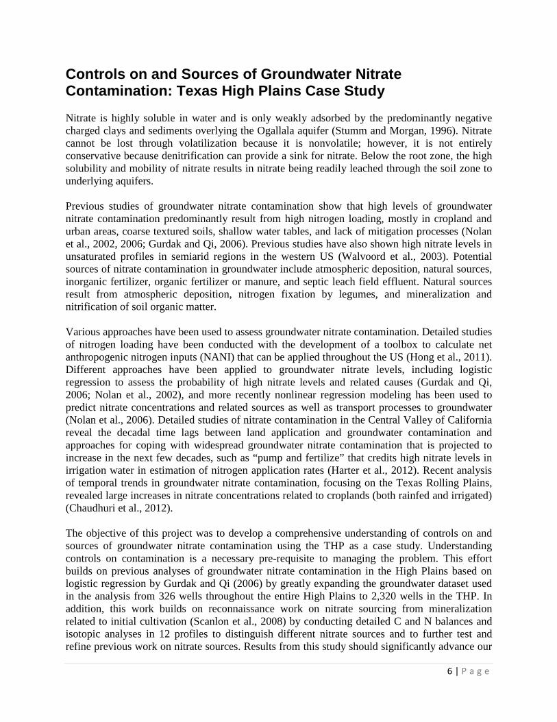
Controls on and Sources of Groundwater Nitrate Contamination: Texas High Plains Case Study Nitrate is highly soluble in water and is only weakly adsorbed by the predominantly negative charged clays and sediments overlying the Ogallala aquifer (Stumm and Morgan, 1996). Nitrate cannot be lost through volatilization because it is nonvolatile; however, it is not entirely conservative because denitrification can provide a sink for nitrate. Below the root zone, the high solubility and mobility of nitrate results in nitrate being readily leached through the soil zone to underlying aquifers. Previous studies of groundwater nitrate contamination show that high levels of groundwater nitrate contamination predominantly result from high nitrogen loading, mostly in cropland and urban areas, coarse textured soils, shallow water tables, and lack of mitigation processes (Nolan et al., 2002, 2006; Gurdak and Qi, 2006). Previous studies have also shown high nitrate levels in unsaturated profiles in semiarid regions in the western US (Walvoord et al., 2003). Potential sources of nitrate contamination in groundwater include atmospheric deposition, natural sources, inorganic fertilizer, organic fertilizer or manure, and septic leach field effluent. Natural sources result from atmospheric deposition, nitrogen fixation by legumes, and mineralization and nitrification of soil organic matter. Various approaches have been used to assess groundwater nitrate contamination. Detailed studies of nitrogen loading have been conducted with the development of a toolbox to calculate net anthropogenic nitrogen inputs (NANI) that can be applied throughout the US (Hong et al., 2011). Different approaches have been applied to groundwater nitrate levels, including logistic regression to assess the probability of high nitrate levels and related causes (Gurdak and Qi, 2006; Nolan et al., 2002), and more recently nonlinear regression modeling has been used to predict nitrate concentrations and related sources as well as transport processes to groundwater (Nolan et al., 2006). Detailed studies of nitrate contamination in the Central Valley of California reveal the decadal time lags between land application and groundwater contamination and approaches for coping with widespread groundwater nitrate contamination that is projected to increase in the next few decades, such as “pump and fertilize” that credits high nitrate levels in irrigation water in estimation of nitrogen application rates (Harter et al., 2012). Recent analysis of temporal trends in groundwater nitrate contamination, focusing on the Texas Rolling Plains, revealed large increases in nitrate concentrations related to croplands (both rainfed and irrigated) (Chaudhuri et al., 2012). The objective of this project was to develop a comprehensive understanding of controls on and sources of groundwater nitrate contamination using the THP as a case study. Understanding controls on contamination is a necessary pre-requisite to managing the problem. This effort builds on previous analyses of groundwater nitrate contamination in the High Plains based on logistic regression by Gurdak and Qi (2006) by greatly expanding the groundwater dataset used in the analysis from 326 wells throughout the entire High Plains to 2,320 wells in the THP. In addition, this work builds on reconnaissance work on nitrate sourcing from mineralization related to initial cultivation (Scanlon et al., 2008) by conducting detailed C and N balances and isotopic analyses in 12 profiles to distinguish different nitrate sources and to further test and refine previous work on nitrate sources. Results from this study should significantly advance our

7 | P a g e
understanding of controls on groundwater nitrate contamination in the THP and assess appropriate techniques for evaluating contamination that should be applicable to many other regions. Project Area Description The THP (94,000 km2 area) includes part of the SHP (57,000 km2 area) and part of the central High Plains (CHP) (37,000 km2 area) of the US High Plains (454,000 km2) (Figure 3). Underlying the High Plains, the Ogallala aquifer is one of the major aquifers in Texas. This aquifer is a major source of water for irrigation, which covers about 12% of the area (Qi et al., 2002). Land use in the THP includes 39% cropland and fallow, 55% grassland/shrubland, and 6% other (Figure 3). Precipitation in the THP ranges from 348 mm/yr in the west to 667 mm/yr in the east (mean 496 mm/yr, PRISM, 1981-2010) (Figure 4). Soil clay content in the shallow subsurface (1.0 – 2.0 m) is predominantly low in the south where soils are mostly sandy and much higher in the north, particularly in the area corresponding to the Pullman clay loam and related soil series (Figure 5). Previous studies of groundwater nitrate contamination in 29 wells screened within 1.5 m of the upper extent of the water table in the SHP showed NO3-N concentrations ranging from 1.0 – 22 mg/L (median 4.1 mg/L) (Stanton and Fahlquist, 2006). High correlations between NO3-N and TDS were attributed to natural and anthropogenic sources of nitrate. Logistic regression analysis applied to the entire High Plains aquifer was used to predict the probability of detecting groundwater nitrate concentrations ≥4 mg/L NO3-N recharged during the past 50 yr based on 336 wells screened near the water table (Gurdak and Qi, 2006). The best fit model includes spatial distribution of nonirrigated and irrigated agricultural lands, soil organic matter and clay content, and depth to the regional water table. Areas with high probability of nitrate contamination include the southern areas of the SHP in Texas, eastern arm of the CHP in Kansas, and southwestern and eastern areas of the NHP in Nebraska. Unsaturated zone studies of nitrate in the SHP show low nitrate inventories in rangeland areas and much higher inventories in rainfed and irrigated agriculture (Scanlon et al., 2008). Much of the higher nitrate inventories under cultivated land were attributed to mineralization of soil organic matter during initial cultivation. High nitrate levels were found at depth corresponding to higher chloride concentrations, indicating old soil water that pre-dated cultivation. Because recharge is the primary mechanism for transporting nitrate from the land surface to the underlying aquifer, previous studies of recharge in the THP are highly relevant for understanding groundwater nitrate contamination. Unsaturated zone studies were used to quantify groundwater recharge under different land use settings, including natural vegetation (rangeland), and rainfed and irrigated cropland (McMahon and Böhlke, 2006; Scanlon et al., 2007, 2010a, b). Rangeland areas are characterized by very low recharge rates, mostly focused beneath ephemeral lakes or playas with most groundwater recharged more than 10,000 yr ago (Pleistocene times) (McMahon et al., 2006). Very sandy soils in parts of the CHP are the exception, with median recharge rates up to 4.8 mm/yr (Scanlon et al., 2010b). Typical recharge rates beneath rainfed cropland range from 5 to 92 mm/yr (median 24 mm/yr) in the SHP and no recharge beneath fine grained soils in the CHP to a median value of 27 mm/yr under coarse grained soils (Scanlon et al., 2010a, b). The range of recharge rates beneath irrigated cropland (18-97 mm/yr) is similar to that under rainfed cropland (5 – 92 mm/yr) but the median is higher under irrigated cropland (41 versus 24 mm/yr)

8 | P a g e
in the SHP. Irrigation in the CHP has increased percolation in all soil types (median 37 mm/yr); however, irrigation return flow has not recharged the aquifer because of deep water tables.
Figure 3. THP study area, land use, and borehole locations. Heavy black line depicts High Plains boundary in Texas and surrounding states. Land use percentages shown represent THP region values only. Irrigated crop area from Qi (2002) and remaining land use based on NLCD (2006). Irrigated crop area was calculated by subtraction from total NLCD crop area (38%), with remainder categorized as rainfed crops.

9 | P a g e
Figure 4. Mean annual precipitation from PRISM 1981 – 2010 data (1 km resolution (www.prism.oregonstate.edu)
Figure 5. Mean soil clay content in the study area based on STATSGO (http://soildatamart.nrcs.usda.gov). Borehole locations and settings from Figure 3 are shown for reference.
Materials and Methods Analysis of Groundwater Nitrate Distribution Groundwater nitrate concentrations were obtained from the Texas Water Development Board (TWDB) groundwater database (www.twdb.state.tx.us). Several aquifers are present in the THP region. The primary aquifer is the Ogallala, which is underlain in different areas by the Edwards-Trinity High Plains, Dockum, and Rita Blanca aquifers (Ashworth and Hopkins, 1995). However, only water wells completed solely in the main body of the Ogallala Aquifer were included in this analysis, excluding wells completed partially or soley in other regional aquifers and in isolated areas of the Ogallala Aquifer occurring outside the main body of the aquifer. Although water quality data in the study area are available beginning in 1937, this study focused on the most recent analyses from data collected between 1988 and 2012 because these data are considered most reliable. Many of the samples during this time were collected under a rigorous quality assurance plan and the Lower Colorado River Authority’s Environmental Laboratory Services (https://els.lcra.org/) performed the majority of the analyses. Only the latest samples for individual wells that are also charge-balanced (i.e., the net cation/anion valence balance is within 10%) are included. For purposes of evaluating long-term trends in nitrate concentrations, data

10 | P a g e
from 1960 to 2012 were assessed using median, 75th, and 90th percentile values of all sample data, grouped by decadal periods, except for the last period representing 2000 to 2012. The selection criteria applied to the recent data available from 2,032 wells which were generally distributed across the area evenly. The mean sample analysis date was 2000. All NO3 concentrations are reported here as equivalent nitrogen (NO3-N) values. For all but 14 samples, NO3-N concentrations were above the detection limit of the analytical method used, which ranged from 0.005 to 1 mg/L NO3-N. All samples were also analyzed for major anions (Cl, SO4, CO3, HCO3), major cations (Ca, Mg, Na, K), and total dissolved solids (TDS). Soil Profiling Soil samples were obtained using a direct-push coring system (Geoprobe 6620DT, Salina, KS) at a total of 65 locations distributed across the region in rangeland (15 profiles), non-irrigated (i.e, rainfed or dryland, 29 profiles), and irrigated (21 profiles) agricultural settings in the THP (Figure 1, Tables 1-3). The boreholes were sampled at various times between 2003 and 2011, to depths ranging from 2.8 to 29 m (mean 10.1 m). Previous evaluation of unsaturated zone nitrate levels was based on 25 profiles restricted to the SHP and 26 profiles in the CHP (Scanlon et al., 2008, 2010a, b). Additional soil samples were collected for C and N analyses in the upper 0.6 m zone in a total of 12 profiles, 5 profiles drilled with a Geoprobe (Model 6620 DT) and 7 profiles drilled using a 35 mm ID bit and a hydraulic soil coring machine (Model 15-TS GSRT, Giddings Machine Co., Windsor, CO). Table 1. Total depths and inventories of Cl and NO3-N in boreholes completed in natural (rangeland) settings. Clay content and presence of Pullman soil series derived from SSURGO.
Borehole Depth (m)
Cl (kg/ha/m)
NO3-N (kg/ha/m)
Clay (%)
Non-Pullman Soils Rob06-02 12.2 23 4.6 25 Whe06-01 11.0 23 32 7 Don06-02 8.4 23 16 13 Hem07-02 12.2 38 0.2 18 And05-02 8.5 736 10 27 Rob07-04 22.6 786 1.6 26 Rob07-01 11.7 883 2.6 27 Hem07-04 10.6 1183 1.3 29 Lyn06-01 29.0 1507 2.5 24 Daw11-01 8.0 1779 18 28 Rob07-06 12.2 2533 5.4 33 Lub11-01 10.3 2805 2.5 17 Daw06-01 8.4 3505 8.9 23 Pullman Soils Pot07-04 14.6 1045 20 42

11 | P a g e
Table 2. Total depths and inventories of Cl and NO3-N in boreholes completed in rainfed (dryland) agricultural settings. Clay content and presence of Pullman soil series derived from SSURGO.
Borehole Depth (m)
Cl (kg/ha/m)
NO3-N (kg/ha/m)
Clay (%)
Non-Pullman Soils Daw03-02 5.0 13 73 23 Daw03-05 4.6 16 25 30 Daw05-01 4.1 8 26 29 Daw06-02 9.3 6 67 24 Daw06-03 7.9 13 53 24 How05-01 6.2 11 125 25 Mar05-01 7.6 8 33 13 Mar05-03 6.6 10 11 26 Bai05-01 11.2 15 24 35 Bai05-02 6.2 39 6 25 Bai06-01 4.7 29 114 26 Gai05-01 5.0 86 38 26 Gai05-02 10.8 13 78 22 Lam05-01 8.6 53 74 25 Mar05-02 9.0 61 139 22 Mar05-04 4.6 40 58 17 Ter05-01 7.2 22 169 23 Hem06-01 9.4 23 8 29 Har08-03 8.9 1061 25 35 Don06-01 15.2 17 3 25 Whe06-02 9.6 7 22 19 She08-02 7.3 23 4 18 Lyn11-02 6.6 16 46 23 Lyn11-03 4.8 47 13 31 Median 7.2 17 33 25 Pullman Soils Arm06-01 8.5 1798 52 44 Pot06-02 13.4 826 22 42 Pot08-04 18.3 809 37 42 Pot08-06 13.7 1229 42 42 Median 13.7 826 37 42
Table 3. Total depths and inventories of Cl and NO3-N in boreholes completed in irrigated agricultural settings. Clay content and presence of Pullman soil series derived from SSURGO.
Borehole Depth (m)
Cl (kg/ha/m)
NO3-N (kg/ha/m)
Clay (%)
Non-Pullman Soils Ter05-03 12.6 914 272 26 Ter08-03 11.8 1974 228 26 Daw08-01 11.9 2431 129 23 Lub08-01 16.7 1262 160 27 Mar08-01 4.9 3528 20 22 Mar08-02 7.4 3755 86 26 Ter05-04 10.2 1609 112 23 Mar08-03 4.3 4371 395 22 Gai08-01 7.9 1317 136 27 Ter08-01 12.2 1206 98 23 Ter08-02 6.5 1395 163 24 She08-01 5.0 481 107 36 Dal08-01 2.8 953 621 25 Hem07-01 10.4 176 12 13 Lyn11-01 10.1 2889 125 24 Median 9.0 1356 127 25 Pullman Soils Pot07-03 18.0 307 134 42 Rob07-02 15.2 663 186 43 Gra06-02 9.8 104 127 42 Pot07-03 18.0 276 121 42 Hal11-02 9.8 195 76 41 Median 15.2 276 127 42

12 | P a g e
Anion concentrations were determined for 1,213 core subsamples by adding double deionized water to the sediment sample in a 1:1 to 2:1 ratio by weight, shaking for 4 h, centrifuging the supernatant, and filtering through 0.45 μm filters. Ion concentrations were analyzed by ion chromatography (Dionex ICS 2000). Ion concentrations are expressed on a mass basis as mg ion per kg of dry soil (=supernatant concentration multiplied by extraction ratio, g water/g soil and divided by water density) and as mg ion per L of soil pore water (= mg/kg divided by gravimetric water content and multiplied by water density). Concentrations on a mass basis are useful for inter-profile comparisons and to reduce variations from differences in soil water contents due to textural variability. Inventories of ions (kg/ha) were calculated by multiplying depth-weighted concentrations (mg/kg) by the interval thickness (m), soil bulk density (kg/m3), and 104 (m2/ha) for units conversion. Approximately 100 samples were analyzed for total C and N from the upper 0.6 m of the profile at 0.05 m intervals to 0.2 m depth, 0.2 - 0.3 m, and 0.3 – 0.6 m (Table 4a-c). These samples were initially air-dried and ground to pass through a 2 mm sieve and stored at 8° C until analyzed. Bulk density was determined using equivalent oven dry sample mass evaluated using water contents calculated for oven dried (24 h) subsamples. Total C and N in soils were determined by dry combustion (900° C) and subsequent differential thermal conductivity analysis of evolved gasses using a Vario Max CN analyzer (Elementar, Inc., Hanau, Germany). Soil samples were analyzed for 2M KCl extractable NO3–N and NH4–N (2 g soil in 20 ml 2M KCl shaken for 0.5 h) using the method described by Keeney and Nelson (1982). A Lachat (Hach Co., Loveland, CO) flow injection autoanalyzer was used to determine analyte concentrations in filtered 2M KCl extracts. Ammonium in extracts was determined using the salicylic analog of the indophenol blue method (EPA, 1983) and NO3 + NO2 in the extracts were determined using the cadmium reduction procedure (EPA, 1983).

13 | P a g e
Table 4a. Rangeland setting borehole sample C and N analysis results.
Borehole Depth NO3-N NH4-N Total N Total C Thickness Bulk Density Total N Total C
cm mg/kg mg/kg mg/kg g/kg m g/cm3 kg/ha Mg/ha
Pot07-04
0-5 15.10 10.11 2393.08 21.63 0.05 1.19 1419.55 12.83 5-10 5.98 7.17 1390.12 12.12 0.05 1.08 753.96 6.57
10-15 5.70 6.63 1298.16 10.33 0.05 1.23 795.40 6.33 15-20 6.30 7.35 1157.46 8.81 0.05 1.33 767.33 5.84 20-30 7.33 5.23 1057.06 7.89 0.10 1.40 1483.88 11.08 30-60 5.71 3.66 824.67 7.34 0.30 1.34 3317.17 29.53
Pot Exc
0-5 17.86 18.52 3515.25 33.80 0.05 1.19 2085.21 20.05 5-10 6.64 8.38 1707.03 16.61 0.05 1.08 925.84 9.01
10-15 5.86 7.30 1559.19 14.13 0.05 1.23 955.34 8.66 15-20 5.27 7.35 1384.12 11.15 0.05 1.33 917.60 7.39 20-30 7.27 6.48 1174.77 9.12 0.10 1.40 1649.11 12.80 30-60 5.50 4.38 884.54 8.02 0.30 1.34 3557.96 32.27
Lub11-01
0-5 5.33 7.45 1806.23 17.55 0.05 1.17 1056.42 5-10 3.46 5.40 1261.20 12.02 0.05 1.29 811.20
10-15 1.56 6.77 1087.95 9.36 0.05 1.25 678.14 15-20 1.80 7.31 1090.88 8.82 0.05 1.19 648.09 20-30 2.15 5.71 1030.09 7.82 0.10 1.37 1406.67 30-60 3.67 8.20 999.34 7.07 0.30 1.46 4366.23
Daw11-01
0-5 1.83 10.38 1542.25 13.99 0.05 1.31 1006.83 5-10 1.07 5.54 1185.10 10.53 0.05 1.43 849.67
10-15 0.76 4.60 1046.15 9.05 0.05 1.31 684.98 15-20 0.59 3.98 1159.29 9.64 0.05 1.30 753.24 20-30 0.57 3.92 1231.89 9.95 0.10 1.02 1258.15 30-60 0.86 6.81 926.63 6.69 0.30 1.48 4127.96
Table 4b. Rainfed setting borehole sample C and N analysis results.
Borehole Depth NO3-N NH4-N Total N Total C Thickness Bulk Density Total N Total C
cm mg/kg mg/kg mg/kg g/kg m g/cm3 kg/ha Mg/ha
Pot06-02
0-5 24.26 14.53 1262.81 9.65 0.05 1.19 749.09 5.73 5-10 6.98 6.98 1128.16 8.76 0.05 1.08 611.88 4.75
10-15 3.48 7.06 1063.26 7.75 0.05 1.23 651.48 4.75 15-20 6.13 5.78 991.45 7.51 0.05 1.33 657.28 4.98 20-30 11.07 4.77 903.30 7.09 0.10 1.40 1268.03 9.96 30-60 8.99 4.55 754.23 6.60 0.30 1.34 3033.82 26.53
Pot08-06
0-5 11.86 10.23 1193.20 9.64 0.05 1.19 707.80 5.72 5-10 4.77 7.98 1132.23 9.15 0.05 1.08 614.09 4.96
10-15 4.02 6.34 1069.12 8.24 0.05 1.23 655.07 5.05 15-20 6.47 5.38 999.20 7.70 0.05 1.33 662.42 5.11 20-30 8.77 7.23 1014.69 7.18 0.10 1.40 1424.40 10.07 30-60 9.39 4.86 798.39 6.29 0.30 1.34 3211.44 25.29
Lyn11-02
0-5 5.44 3.59 455.89 2.53 0.05 1.47 335.87 1.87 5-10 2.00 2.67 469.92 2.38 0.05 1.55 363.42 1.84
10-15 1.39 3.07 470.03 2.36 0.05 1.49 349.32 1.76 15-20 1.37 5.40 479.55 2.56 0.05 1.42 341.56 1.82 20-30 1.61 2.64 418.90 2.53 0.10 1.59 664.20 4.02 30-60 1.10 6.05 697.31 7.01 0.30 1.37 2873.65 28.88
Lyn11-03
0-5 7.40 6.38 708.90 6.53 0.05 1.47 522.28 5-10 2.72 4.24 699.83 6.36 0.05 1.55 541.22
10-15 1.33 4.01 583.54 5.53 0.05 1.49 433.68 15-20 1.00 4.08 678.43 5.56 0.05 1.42 483.21 20-30 1.04 3.78 775.12 7.17 0.10 1.59 1229.02 30-60 0.97 7.60 764.69 9.50 0.30 1.37 3151.34

14 | P a g e
Soils were analyzed for δ13C, δ15N, %C, and %N using a Carlo Erba EA-1108 (CE Elantech, Lakewood, NJ) interfaced with a Delta Plus (ThermoFinnigan, San Jose, CA) isotope ratio mass spectrometer operating in continuous flow mode (Table 5). C and N isotope ratios are presented in δ notation:
δ = [(RSAMPLE – RSTD)/RSTD] x 103 (Eq. 1) where RSAMPLE is the 13C/12C or 15N/14N ratio of the sample and RSTD is the 13C/12C ratio of the V-PDB standard (Coplen, 1996) or the 15N/14N ratio of atmospheric N2 (Mariotti, 1983). Precision of duplicate measurements was 0.10 ‰ for δ13C, 0.15 ‰ for δ15N, 0.03 for %N, and 0.14 for %C. Table 4c. Irrigated setting borehole sample C and N analysis results.
Borehole Depth NO3-N NH4-N Total N Total C Thickness Bulk Density Total N Total C
cm mg/kg mg/kg mg/kg g/kg m g/cm3 kg/ha Mg/ha
Pot08-02
0-5 299.02 36.44 1908.15 13.07 0.05 1.19 1131.89 7.75 5-10 47.40 15.12 1650.68 13.07 0.05 1.08 895.28 7.09
10-15 28.36 14.18 1353.26 10.18 0.05 1.23 829.16 6.24 15-20 19.17 12.97 1111.82 8.27 0.05 1.33 737.07 5.48 20-30 17.48 9.07 1011.47 7.03 0.10 1.40 1419.87 9.87 30-60 20.43 5.84 788.05 6.88 0.30 1.34 3169.87 27.67
Pot08-03
0-5 165.79 22.39 1937.94 14.38 0.05 1.19 1149.57 8.53 5-10 22.06 10.99 1451.47 11.56 0.05 1.08 787.23 6.27
10-15 16.20 12.89 1230.22 9.14 0.05 1.23 753.77 5.60 15-20 7.04 13.13 1071.22 7.45 0.05 1.33 710.16 4.94 20-30 3.79 10.96 904.24 7.09 0.10 1.40 1269.35 9.95 30-60 6.94 8.11 772.95 6.90 0.30 1.34 3109.12 27.77
Pot08-09
0-5 99.70 27.94 1743.90 12.50 0.05 1.19 1034.46 7.42 5-10 31.21 14.52 1397.28 10.23 0.05 1.08 757.84 5.55
10-15 18.26 9.58 1166.40 7.89 0.05 1.23 714.67 4.83 15-20 20.79 13.40 1116.83 7.20 0.05 1.33 740.40 4.77 20-30 13.53 6.98 962.96 6.52 0.10 1.40 1351.78 9.15 30-60 10.12 5.20 789.87 7.45 0.30 1.34 3177.19 29.95
Lyn11-01
0-5 27.05 29.63 532.04 3.11 0.05 1.47 391.98 2.29 5-10 9.05 2.66 528.79 3.04 0.05 1.55 408.95 2.35
10-15 7.23 2.99 446.42 2.64 0.05 1.49 331.77 1.96 15-20 4.73 2.37 463.13 2.53 0.05 1.42 329.86 1.80 20-30 5.57 2.46 472.83 2.38 0.10 1.59 749.71 3.78 30-60 6.68 4.01 516.68 3.03 0.30 1.37 2129.28 12.49
Hal11-02
0-5 100.41 72.42 1910.96 15.41 0.05 1.19 1139.67 5-10 19.44 4.21 1137.12 9.17 0.05 1.34 764.65
10-15 14.67 8.90 990.77 7.17 0.05 1.45 720.00 15-20 6.75 3.92 927.98 6.43 0.05 1.34 619.97 20-60 10.73 8.26 789.21 12.13 0.40 1.27 4001.54

15 | P a g e
Table 5a. Rangeland setting borehole sample N and C isotope analysis results. Bore-hole
Sub-sample
Depth d15N d13C N C (cm) (‰) (‰) (%) (%)
Pot07-04
A
0-5 5.52 -20.11 0.30 3.08 5-10 7.33 -16.96 0.15 1.39 10-15 8.31 -15.01 0.12 1.04 15-20 8.48 -14.97 0.11 0.97 20-30 9.08 -14.77 0.09 0.85 30-60 8.68 -14.89 0.07 0.81
B
0-5 5.97 -18.52 0.22 2.16 5-10 7.34 -16.48 0.12 1.21 10-15 8.15 -14.97 0.11 1.03 15-20 8.57 -14.33 0.09 0.83 20-30 8.60 -14.76 0.08 0.78 30-60 8.49 -15.71 0.07 0.81
Pot Exc
A
0-5 5.35 -17.99 0.37 4.17 5-10 6.54 -14.18 0.17 1.64 10-15 7.53 -13.51 0.16 1.47 10-15 Dup
7.67 -13.46 0.15 1.38
15-20 8.03 -13.17 0.13 1.23 20-30 8.47 -13.16 0.11 0.95 20-30 Dup
8.57 -13.19 0.10 0.90
30-60 8.57 -13.78 0.07 0.80
B
0-5 5.12 -17.15 0.32 3.44 0-5 Dup
5.24 -17.59 0.35 3.87
5-10 6.28 -15.02 0.16 1.66 5-10 Dup
6.38 -15.25 0.16 1.70
10-15 7.40 -14.13 0.14 1.44 15-20 8.23 -13.13 0.11 1.09 20-30 8.28 -13.85 0.10 0.98 30-60 8.42 -14.15 0.07 0.92
Lub11-01
A
0-5 6.30 -17.40 0.23 2.46 5-10 6.55 -15.90 0.15 1.62 10-15 6.83 -15.18 0.13 1.38 15-20 6.57 -14.28 0.10 1.35 20-30 7.48 -13.52 0.10 1.32 20-30 Dup
7.97 -13.36 0.09 1.22
30-60 7.89 -15.01 0.08 0.89
B
0-5 6.25 -17.31 0.17 2.26 5-10 6.43 -15.71 0.14 1.97 10-15 6.90 -14.36 0.10 1.36 15-20 6.82 -14.49 0.10 1.53 20-30 8.06 -13.05 0.09 1.11
Table 5b. Rainfed setting borehole sample N and C isotope analysis results. Bore-hole
Sub-sample
Depth d15N d13C N C
(cm) (‰) (‰) (%) (%)
Pot06-02
A
0-5 6.82 -16.46 0.10 0.93
5-10 7.50 -15.95 0.09 0.85
10-15 7.71 -14.57 0.09 0.79
15-20 8.10 -13.57 0.09 0.79
20-30 8.66 -12.62 0.08 0.72
30-60 8.91 -13.74 0.06 0.74
B
0-5 5.59 -16.59 0.10 0.92
5-10 6.43 -16.02 0.09 0.95
10-15 7.50 -14.34 0.08 0.80
15-20 7.86 -13.15 0.09 0.75
20-30 8.13 -12.12 0.07 0.72
30-60 8.74 -13.60 0.06 0.75
Pot08-06
A
0-5 7.04 -15.95 0.11 0.94
5-10 7.01 -16.09 0.10 0.96
10-15 7.99 -14.34 0.10 0.87
15-20 8.39 -13.38 0.08 0.78
20-30 9.11 -13.10 0.08 0.72
30-60 9.15 -13.55 0.06 0.79
B
0-5 6.72 -16.15 0.10 0.96
5-10 7.44 -15.26 0.09 0.90
10-15 8.36 -13.25 0.09 0.82
15-20 8.95 -12.88 0.09 0.76
20-30 8.92 -13.12 0.08 0.72
30-60 9.03 -13.75 0.07 0.79
Lyn11-02
A
0-5 7.53 -16.93 0.04 0.41
5-10 7.34 -16.83 0.04 0.36
10-15 7.40 -17.01 0.04 0.37
15-20 7.68 -16.67 0.04 0.39
15-20 Dup
7.48 -16.87 0.04 0.39
20-30 7.43 -16.26 0.04 0.38
30-60 7.84 -14.39 0.06 0.59
B
0-5 7.64 -16.08 0.03 0.23
5-10 7.78 -15.50 0.02 0.21
10-15 7.97 -16.39 0.03 0.24
15-20 7.55 -19.31 0.03 0.35
20-30 7.29 -16.42 0.03 0.23

16 | P a g e
Table 5c. Irrigated setting borehole sample N and C isotope analysis results. Bore-hole
Sub-sample
Depth d15N d13C N C (cm) (‰) (‰) (%) (%)
Pot08-02
A
0-5 7.88 -17.57 0.20 2.11 5-10 8.12 -17.83 0.16 1.82 10-15 8.00 -17.33 0.14 1.68 15-20 7.70 -16.78 0.12 1.38 20-30 8.23 -14.72 0.08 0.73 30-60 7.65 -14.29 0.06 0.76
B
0-5 8.50 -18.11 0.23 2.48 5-10 8.46 -17.93 0.17 1.91 10-15 7.77 -17.31 0.13 1.54 15-20 7.57 -16.47 0.11 1.26 20-30 7.89 -14.80 0.08 0.71 30-60 8.47 -14.35 0.06 0.73
Pot08-03
A
0-5 8.87 -17.66 0.21 2.32 5-10 7.17 -18.72 0.15 1.79 10-15 6.80 -17.59 0.12 1.43 15-20 6.98 -16.41 0.10 1.16 20-30 7.99 -13.74 0.08 0.71 30-60 7.91 -15.11 0.08 0.72
B
0-5 9.14 -18.40 0.23 2.65 0-5 Dup 8.78 -18.52 0.22 2.41 5-10 6.74 -18.67 0.13 1.13 10-15 6.38 -17.77 0.11 0.91 15-20 6.85 -16.52 0.09 0.77 15-20 Dup
6.98 -16.64 0.09 1.05
15-20 Dup
6.82 -13.72 0.09 0.93
20-30 8.32 -13.77 0.08 0.71 20-30 Dup
8.37 -13.63 0.08 0.70
30-60 8.90 -15.05 0.07 0.67 30-60 Dup
8.21 0.06
Pot08-09
A
0-5 8.82 -17.87 0.18 2.04 5-10 7.64 -17.89 0.13 1.53 10-15 7.70 -16.59 0.11 1.20 15-20 7.41 -16.29 0.10 1.14 20-30 8.87 -14.20 0.08 0.66 30-60 8.43 -14.12 0.09 0.70
B
0-5 8.71 -17.31 0.18 1.42 5-10 7.93 -17.64 0.12 1.05 10-15 7.66 -15.89 0.10 0.81 15-20 7.46 -16.50 0.09 0.73 20-30 8.58 -13.99 0.08 0.67 30-60 8.77 -13.99 0.06 0.72
Bore-hole
Sub-sample
Depth d15N d13C N C
(cm) (‰) (‰) (%) (%)
Hal11-02
A
0-5 5.41 -19.35 0.20 2.42 5-10 6.43 -18.12 0.13 1.36 5-10 Dup
6.32 -18.49 0.14 1.46
10-15 7.29 -15.18 0.11 1.07 15-20 6.86 -15.83 0.10 1.04 20-60 7.21 -14.58 0.08 0.78
B
0-5 6.31 -19.70 0.19 2.58 5-10 6.68 -17.20 0.10 1.24 10-15 7.26 -16.34 0.08 0.73 15-20 7.32 -14.38 0.07 0.64
Lyn11-01
A
0-5 6.54 -21.21 0.05 0.47 5-10 7.33 -19.83 0.04 0.44 10-15 7.36 -18.57 0.03 0.32 15-20 7.28 -18.24 0.04 0.34 20-30 7.43 -18.06 0.04 0.35 30-60 8.09 -14.09 0.05 0.43
B
0-5 6.60 -20.08 0.03 0.27 5-10 7.07 -20.40 0.03 0.30 10-15 7.18 -18.37 0.03 0.23 15-20 7.71 -17.98 0.03 0.24 20-30 7.63 -17.50 0.03 0.23

17 | P a g e
Data Analysis Indicator Kriging The spatial distribution of groundwater NO3-N was characterized using indicator kriging to produce a map depicting the probability that NO3-N would exceed a pre-specified background level. Indicator kriging uses transformed values to produce maps that estimate the probability of exceeding the background or a given threshold value. The primary advantages of using indicator kriging in this application are that it does not require a priori assumption regarding the normality of the data distribution and that it can incorporate non-detect or “less-than” values (though limited in this case) that are less than or equal to the threshold concentration. Concentration values were assigned a value of “1” if greater than the threshold concentration and a value of “0” if less than or equal to the threshold. Logistic Regression Logistic regression is widely used in social sciences research and for epidemiological studies to assess risk. The use of logistic regression to produce probability maps of groundwater contamination with potential explanatory variables has increased in the past decade and has been used in several national assessments of nitrate and pesticide contamination (Nolan et al., 1998; 2002; Nolan and Stoner, 2000; Nolan, 2001) and also in evaluation of nitrate contamination in recently recharged groundwater (≤50 yr old) in the High Plains (Gurdak and Qi, 2006). The logistic regression approach frequently used to evaluate nitrate contamination has been to represent groundwater nitrate concentration as a bivariate, dependent variable by selecting a threshold or background nitrate concentration to represent nitrate concentrations that exceed natural background levels. Background nitrate concentrations in the area have ranged from 2 mg/L (Rupert, 1998); 3 mg/L (Squillace et al., 2002), 4 mg/L (Nolan, 2002), and 5 mg/L (Rupert, 2003) in different studies. Groundwater nitrate concentrations are then related to various explanatory variables that include nitrogen loading (atmospheric deposition, organic and inorganic fertilizer application, nitrogen fixation, septic leach field effluent) and parameters related to loading (precipitation, irrigation), ability of soils to transmit contaminants from the land surface (well drained soils, land surface slope, clay content, and soil organic matter), and aquifer characteristics (depth to water, saturated thickness). Logistic regression is used to predict binary dependent variables using independent variables. It also assesses the percent of variance in the dependent variable (nitrate exceeding background level) that can be explained by the independents and simultaneously determines the relative importance of different independent variables evaluated (Kleinbaum, 1994; Hosmer and Lemeshow, 2001). One of the primary differences between logistic regression and ordinary least squares linear regression is that the dependent variable is the probability of being in a category (i.e. ≥4 mg/L NO3) rather than the measured value of the dependent variable. Ordinary least squares linear regression cannot be used with binary dependent variables because residuals have to be normally distributed and binary variables do not fit this requirement. Logistic regression is much less stringent than ordinary least squares regression. It does not assume a linear relationship between the independent and dependent variables, or require variables to be normally distributed, and does not require homoscedasticity (uniform variance with X). Ordinary regression is used to predict a continuous dependent variable from one or many independent

18 | P a g e
variables (x, predictors) by finding values of b0, b1, b2 etc. ...** 221 +++= xbxbay (Eq. 2)
Logistic regression is used when the dependent variable is limited to 2 values (e.g. presence or absence of nitrate concentrations with respect to a threshold concentration, 2, 3, 4, or 5 mg/L). However, ordinal models can be used when more than one threshold value is considered in the analysis. The resultant equation from logistic regression is used to determine the probability of occurrence of the dependent variable as a function of the independent variables. The odds ratio is the probability of occurrence of an event, e.g. probability of exceeding a background value, divided by the probability of the event not occurring.
PPratioOdds−
=1 (Eq. 3)
The odds ratio provides information on the number of times the outcome occurs or does not occur when the predictor is increased by 1 unit. The odds ratio is constrained between 0 and 1. To make the odds of an event occurring relative to the odds of an event not occurring symmetrical, the natural log is used. If P is > 0.5, ln(P/1-P) is positive whereas if P < 0.5, ln(P/1-P) is negative. In logistic regression, the dependent variable is a logit (i.e. natural log of the odds ratio) (Helsel and Hirsch, 1992):
−
==P
PPitratioodds1
ln)(log)ln( (Eq. 4)
In logistic regression, logit (P) is a linear function of the independent variables. Odds ratios can be converted back to probabilities as follows:
)(0 00
00
11
1;
1;
1ln bXbbXb
bXbbXb
ePor
eePe
PPXbb
PP
+−+
++
+=
+==
−+=
− (Eq. 5)
where P is probability of a 1 or the occurrence of a contaminant concentration greater than a threshold value in our case. The last 2 expressions for P represent the logistic transform. If ln(odds) is linearly related to X, then P and X are nonlinearly related and form an S shaped curve. The variance, P(1-P), is not constant with X (i.e. not homoscedastic) and is a maximum at P = 0.5 and approaches zero as P approaches 1 or 0. Model parameters are generally selected to maximize the goodness of fit between the measured and simulated values. In ordinary least squares regression, the sum of squared distances of the data points to the regression line are minimized to estimate the coefficients in the regression equation. In logistic regression, there is no mathematical solution to produce least squares estimates of parameters. Maximum likelihood estimation optimizes the fit by maximizing the log likelihood (LL) which represents how likely it is (the odds that the measured values of the dependent variable may be predicted from the measured values of the independent variables). A likelihood is a conditional probability (e.g. P(Y|X) the probability of Y given X) or probability of

19 | P a g e
the measured values of the dependent variable may be predicted from the observed values of the independent variables. The likelihood varies from 0 to 1 like any probability. Because the probability is a small number, the natural log of this number is used which varies from 0 to minus infinity. The resulting natural log is generally multiplied by -2 to make the number positive. The null hypothesis is that the LL coefficients are zero. Therefore, increased values of the statistic -2LL (-2 log likelihood) represents a worse fit. An iterative process is used to determine the parameters of the logistic regression (i.e. b0 and b) to maximize the likelihood (conditional probability of the data given parameter estimates) of the sample data until convergence is achieved. When large samples are used, -2LL is chi-square distributed. The log-likelihood test of a model (also called the model chi-square test, likelihood ratio test, or G statistic) tests the statistical significance of coefficients in the logistic regression model (Hosmer and Lemeshow, 2001):
)(2 modint elLLG −−= (Eq. 6) where Lint is log-likelihood of intercept only and Lmodel is log-likelihood of model with explanatory variables. The G statistic is chi square distributed and the null hypothesis is that the slope coefficients for the explanatory variables are 0. The G statistic is used to compare predicted values with observed values of the dependent variable with and without different explanatory variables. A well-fitting model will have a low p value (e.g. <0.05). The Wald statistic can be used to test the significance of individual logistic regression coefficients for independent variables. The Wald statistic is approximately equal to the L statistic for large samples and is the ratio of the unstandardized logit coefficient to its standard error. If logit coefficients are large, the standard error is inflated which lowers the Wald statistic and may result in false negatives (i.e. effect not significant when it is) (Menard, 2002). The Hosmer and Lemeshow’s (HL) goodness of fit test provides a test of the overall model (Hosmer and Lemeshow, 2001). The HL test differs from the G statistic in that only one model is evaluated in the HL test whereas the G statistic compares models with and without specific explanatory variables. The data are divided into deciles based on predicted probabilities and chi squares are computed from observed and expected frequencies. A probability value is calculated from the chi square distribution with 9 degrees of freedom to test the fit of the logistic regression model. The null hypothesis is that the model fits the data; therefore, higher p values indicate a better fit. The goodness of fit was also evaluated using linear regression of predicted probabilities for deciles of risk used to calculate the HL statistic versus observed probabilities of elevated nitrate concentrations. Higher coefficients of determination (R2) values indicate better fits. In addition, predicted and observed probabilities were plotted and compared with a 1:1 line with a zero intercept. A perfect fit between predicted and observed probabilities would plot along the 1:1 line. Explanatory Variables Evaluated in Logistic Regression A variety of potential explanatory variables were examined in this study, including those

20 | P a g e
reflecting nitrate loading as well as soil and hydrogeologic attributes affecting contamination. To minimize collinearity impacts, variables that were correlated with each other were represented by a single representative variable where possible. Although several variables used in the logistic regression related to soils examined from the STATSGO (USDA, 1994) database (soil thickness, permeability, organic matter, available water capacity, drainage, surface slope), most were related to soil clay content. A map of average clay content in the upper 1.0 to 2.0 m (Figure 3) shows the general trend of high clay content in the CHP decreasing toward and into the SHP. Clay content is generally related to the underlying geology. Other variables were examined initially, but the final set of variables examined in the univariate logistic regression analysis is listed in Table 6. The variables can be broadly divided into three categories; nitrogen loading and related parameters, intrinsic susceptibility to contamination related to soil, and aquifer properties. Table 6. Univariate logistic regression analysis results, including standardized estimates and p-values of individual variables related to the probability of NO3-N exceeding 2.5 mg/L in the north region and 4 mg/L in the south region. Bold values indicate variables having p-values smaller than ~0.2. Larger standardized estimates tend to have smaller p-values.
Variable Explanation North model South model Est. Std. p-value Est. Std. p-value
Natural Natural land 1 km2 area (%) -0.0061 -0.1181 0.1710 -0.0209 -0.4150 0.0023 Irrigated Irrigated land 1 km2 area (%) 0.0066 0.0488 0.1334 0.0130 0.1555 0.0283 Agricultural Agricultural land 1 km2 area (%) -0.0020 -0.0388 0.7463 -0.0004 -0.0084 0.9614 FertN County average fertilizer loading (kg-N/ha/yr) 0.0128 0.1215 0.2012 0.0023 0.0186 0.8674 ManN County average manure loading (kg-N/ha/yr) 0.0062 0.0487 0.2925 0.0072 0.0224 0.7094 Fertilizer FertN applied only to Ag area (kg-N/ha/yr) -0.0057 -0.0497 0.6675 -0.0076 -0.0556 0.7176 Precip Average annual precipitation (m/yr) -2.9496 -0.0888 0.0664 -1.3810 -0.0300 0.7023 DTW Depth to water table (m) -0.0070 -0.1141 0.0191 -0.0677 -0.5614 <0.0001 Sthk Aquifer saturated thickness (m) -0.0002 -0.0023 0.9582 -0.0031 -0.0167 0.7574 AvgClay Soil clay content percent (%) -0.0526 -0.2640 <0.0001 0.0435 0.0990 0.1371 Est: Estimate, Std: Standardized Estimate Sources of nitrate include inorganic fertilizer (Fertilizer), organic fertilizer (manure), atmospheric deposition, and natural N fixation, which are found in the NANI toolbox (Hong et al., 2011). Databases used in NANI include county-level Agricultural Census data for 1987, 1992, 1997, 2002, and 2007 (http://www.agcensus.usda.gov/), county-level Census data for the population in Census years 1990 and 2000 (http://www.census.gov/), county-level USGS fertilizer application from 1987 to 2001 (Ruddy et al. 2006) and 2002 - 2006, and N deposition data from Community Multiscale Air Quality from 2002 to 2006 (Schwede et al., 2009). Parameters related to N loading include precipitation from PRISM (mean annual precipitation 1981 – 2010) (Figure 4) and irrigation from Qi et al. (2002). Land cover data (natural and cropland) were based on the 2006 National Land Cover Data (NLCD) (Figure 3) and water table depths (Figure 6) were obtained from Texas Commission on Environmental Quality (TCEQ) Source Water Assessment and Protection (SWAP) program (http://www.tceq.texas.gov/drinkingwater/SWAP). This data was used to calculate aquifer saturated thickness using water table elevation and Ogallala aquifer base depth information. Gurdak and Qi (2006) calculated the 90 degree contributing area to each of the 326 wells used in their analysis for the entire High Plains aquifer based on the groundwater flow regime; however,

21 | P a g e
the contributing area used in this study was based on a 1 km² area surrounding the well location points.
Figure 6. Depth to water table in the High Plains Aquifer study area based on data from the TCEQ SWAP database. The THP is divided into north and south regions by the NW-SE trending line representing the 500 mg/L total dissolved solids (TDS) contour separating higher TDS concentrations to the south (median 874 mg/L, 751 wells) from lower TDS concentrations to the north (median 356 mg/L, 1,281 wells). The aquifer is traditionally divided into geographic regions defined as the CHP and SHP regions separated where the outcrop area is narrowest in the central Texas panhandle region. The 500 mg/L TDS subdivides the THP into a shallow water table zone in the south region (median depth 26 m) from a deeper water table zone in the north region (medial depth 62 m).
Logistic Regression Model Development The relationship between NO3-N concentrations exceeding the background value and individual explanatory variables was evaluated (Table 6). Different units apply to the various explanatory variables so their coefficients were standardized to facilitate direct intercomparisons among explanatory variables. The standardization of the logistic regression coefficients involved multiplication by the standard deviation of the explanatory variable, by the square root of the correlation coefficient and dividing by the standard deviation of the estimated logit (×SDx × r/SDy) technique (Menard, 2002; Gurdak and Qi, 2006). Multivariate models were then developed using both forward (stepwise) and backward elimination techniques. Forward modeling is performed by sequentially adding variables in a stepwise fashion, starting with the most significant variable. At each step, the significances of the remaining variables are calculated and the most significant remaining variable is then included in the next model. This process continues until all of the variables have been sequentially examined in relation to the (growing) combined model. Also, during the process, a pre-specified threshold significance level is used to determine if a variable can be included in the model. A threshold (model entry) value of 0.4 was used in this analysis. Backward elimination modeling is essentially the reverse of the forward process, where all of the variables are initially included and the least significant variable is eliminated sequentially. Again, a threshold (model exit) elimination value of 0.1 was used in this analysis. Both the entry and exit threshold values are consistent with those used by Gurdak and Qi (2006).

22 | P a g e
Analysis of Nitrogen Mineralization and Nitrification Sources of high NO3–N in boreholes beneath cultivated land (Figure 3) include both mineralized nitrogen (Scanlon et al., 2008) and applied N-fertilizer. Analysis of mineralization/nitrification of soil organic N as a source of groundwater nitrate included evaluation of old nitrate dated using application of the chloride mass balance equation to soil water as described in Scanlon et al. (2008). This old nitrate is generally found at depth in unsaturated zone profiles. Additional unsaturated zone profiles drilled in this study sampled for soil organic carbon and nitrogen in adjacent noncultivated plots where available to assess this source of nitrate. A detailed management record (1927 – present) of rainfed cultivated plots at the USDA-ARS Conservation and Production Research Laboratory in Potter County, Texas was available and provided the rare opportunity to evaluate mineralization of soil organic nitrogen (SON). Sampled plots are situated in Pullman clay loam soil in the CHP have never been fertilized since they were first cultivated in 1919. In 1921, the plots were returned to native vegetation until 1927 when cultivation again resumed (Johnson and Davis, 1972). From this point on, the plots have been in continuous cultivation with no N fertilizer amendments throughout their entire history. The cropping system consisted of continuous wheat or wheat-fallow rotation (1927 – 1948) and wheat-sorghum-fallow rotation (1949 – present). Yields for wheat and sorghum were reported in 57 and 64 years respectively out of a possible 86 years (Johnson and Davis, 1972; Jones and Popham, 1997; Unger and Baumhardt, 1999). The impact of land use changing from native rangeland to cropland at this site was estimated to assess mineralization/nitrification as a source of nitrate in the system. To accomplish this, a N balance was constructed using long-term yield records for the applied crop rotations along with near surface and entire soil profile sampling of the N inventory under unfertilized rainfed cropland and adjacent native grassland vegetation. Increases in profile N are balanced by the N in crop biomass exported off of the site in the form of grain, hay, and fiber. Results and Discussion Spatiotemporal Distribution of Groundwater Nitrate Groundwater nitrate concentrations are highly variable spatially (Figure 7). Over the entire THP, 9% of recently sampled wells (latest sample between 1988 and 2012) exceed the EPA MCL of 10 mg/L NO3-N. Most of the contaminated wells are located in a zone of high total dissolved solids (TDS ≥500 mg/L) in the southern region of the THP, where 23% of the wells exceed the MCL. In contrast, only 1% of wells exceed the MCL in the north region. Much of the results section of this report includes reference to this south region with high TDS and is distinct from the geographic SHP region (Figures 6 & 7). The north region refers to the remaining area of the THP outside this zone of high TDS in the south. Nitrate-N concentrations are distinctly higher in the south (4.8 mg/L) relative to the north (1.9 mg/L) (Figure 8). There are no differences in NO3-N distributions among the different well use categories (domestic, irrigation, municipal) in the north region; however, the median concentration for domestic wells (6.5 mg/L) in the south is 150% higher than that for other well uses combined (4.4 mg/L). Domestic well make up 30% of all wells in that region. The higher NO3-N concentrations associated with domestic wells may result from the shallower depths of domestic wells (median 24 m deep) relative to irrigation
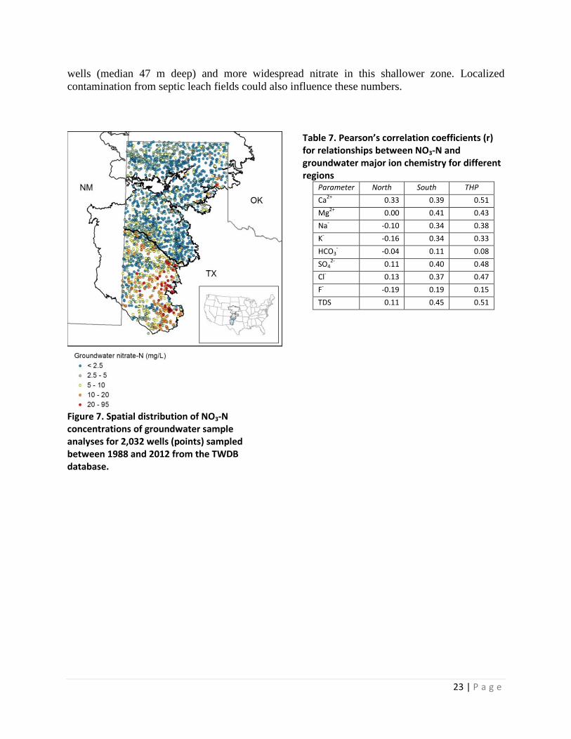
23 | P a g e
wells (median 47 m deep) and more widespread nitrate in this shallower zone. Localized contamination from septic leach fields could also influence these numbers.
Figure 7. Spatial distribution of NO3-N concentrations of groundwater sample analyses for 2,032 wells (points) sampled between 1988 and 2012 from the TWDB database.
Table 7. Pearson’s correlation coefficients (r) for relationships between NO3-N and groundwater major ion chemistry for different regions
Parameter North South THP Ca2+ 0.33 0.39 0.51 Mg2+ 0.00 0.41 0.43 Na- -0.10 0.34 0.38 K- -0.16 0.34 0.33 HCO3
- -0.04 0.11 0.08 SO4
2- 0.11 0.40 0.48 Cl- 0.13 0.37 0.47 F- -0.19 0.19 0.15 TDS 0.11 0.45 0.51

24 | P a g e
Figure 8. Groundwater NO3-N distributions a) for all wells in the north and south regions and b) different well uses in the south region. Median NO3-N concentration in the south (4.8 mg/L) is 250% greater than in the north (1.9 mg/L). Within the south region, the median concentration for domestic wells (6.5 mg/L), which represent 30% of all wells in the south, is 150% greater than for all other well uses combined (4.4 mg/L).
Figure 9. LOWESS plots of groundwater nitrate-N concentrations versus well depth in the a) northern and b) southern regions of the study area. Vertical dashed lines represent the 10 mg/L NO3-N MCL and the 2.5 mg/L (a) and 4 mg/L (b) threshold concentrations used in indicator kriging.
Depth Variations in Nitrate Concentrations Concentrations of NO3-N vary with total well depth as illustrated in Figure 9 by the locally-weighted, smoothed scatterplot (LOWESS, Cleveland, 1981). The regional variations in NO3-N with well depth reflect the spatial variation in well depths and water table depths between the south (high TDS) and north regions (low TDS). Focusing on the high NO3-N zone in the south shows that NO3-N concentrations also tend to decrease significantly as well depth increases, most likely reflecting input of NO3-N from the unsaturated zone. The 1% of wells exceeding the EPA MCL in the north region are almost exclusively shallower wells with depths similar to those

25 | P a g e
found in the south. The LOWESS plot values for the deepest wells in both regions give an indication of appropriate “background concentrations” which refer to concentration levels attributed to natural, i.e. “nonanthropogenic” processes: 2.5 mg/L in the northern region and 4 mg/L in the southern region. Gurdak and Qi (2006) selected a value of 4.0 mg/L NO3-N throughout the SHP and CHP to include the range of background concentrations from the paloerecharge (1.9 – 3.5 mg/L; McMahon et al., 2004). Probability Map of Groundwater Nitrate Concentrations In addition to the point map of groundwater NO3-N concentrations, the spatial distribution of nitrate contamination is also represented by a probability of exceeding the selected threshold of NO3-N concentrations using indicator kriging (Figure 10). The threshold values of 2.5 mg/L NO3-N in the north region and 4 mg/L in the south region approximately represent the respective 75th percentile distribution values and are consistent with the deeper NO3-N concentrations from the LOWESS plots in these regions (Figure 9). Thus, high probability values represent regions where groundwater NO3-N concentrations are generally highest. The 60% or greater probability of exceeding the background level (4 mg/L) in the south region extends over 49% of the area whereas the 80% or greater probability extends over 19% of the area. In contrast, the 60% or greater probability of exceeding 2.5 mg/L in the north extends over only 9% of the area with the 80% or greater probability being limited to 1% of the area. Because domestic wells have higher NO3-N concentrations in the south, the impact of these wells was separately investigated in the indicator kriging by excluding domestic wells in the south region from the analysis; however, these results were not significantly different from those obtained using all the data. The point concentration and probability concentration maps show similar regional trends; however, the latter tends to smooth-out hotspots of contamination related to single wells that may result from local contamination and not reflect a regional trend. Therefore, the kriged probability map (Figure 10) is considered more representative of the regional nitrate distribution than the well point location map (Figure 7). Temporal Variability in Groundwater Nitrate Concentrations Groundwater NO3-N concentrations have increased with time, with overall higher concentrations and greater increases in the south relative to the north (Figure 11). From the 1960s when widespread groundwater sampling began to the 2000s, median NO3-N increased from 1.5 to 1.9 mg/L (31% increase) and the 90th percentile increased from 2.7 to 4.9 mg/L (85% increase) in the north. During the same time period, median NO3-N increased from 1.2 to 5.1 mg/L (310% increase) and the 90th percentile increased from 3.2 to 15.9 mg/L (400% increase) in the south. Controls on Groundwater Nitrate Contamination Logistic Regression Analysis The univariate logistic regression analysis reveals that significantly correlated explanatory variables (p ≤0.2) for high nitrate, NO3-N ≥4 mg/L, include natural and irrigated land, depth to water and average clay content in the south (Table 6). Similar variables were found for the north region with the addition of inorganic N fertilizer and precipitation.

26 | P a g e
Figure 10. Spatial probability of groundwater NO3-N exceeding background concentrations of 4.0 mg/L in the south and 2.5 mg/L in the north regions of the study area based on indicator kriging of groundwater sample analyses for 2,032 wells (points) sampled between 1988 and 2012. Stable variogram models were fitted to the data with lag distances of 2.5 km (south) and 5.1 km (north), major range distances of 13.2 km (south) and 61.2 km (north), and anisotropy ratios of 1.2 (south) and 1.8 (north).
Figure 11. Temporal trends in groundwater nitrate-N concentration distributions since 1960 in the a) north and b) south regions of the study area. Points represent the 50th, 75th, and 90th percentiles of concentration for samples pooled by decadal time intervals. Values at the tops of the graphs represent the numbers of samples in each decade.
The initial multivariate logistic regression model included all the data from the north and south regions; however, the Hosmer-Lemeshow (2001) fit was poor (p<0.01; a p value > 0.05 is a good fit). As a result, separate models were developed for each region. The best multivariate model for the south region included, in order of importance, depth to water table, and percents of both natural and irrigated land within the surrounding 1 km2 grid (Table 8). The negative correlation with percent natural land indicates that decreasing natural land increases the probability of groundwater contamination whereas the positive correlation with irrigation land indicates that increasing irrigated land increases the probability of nitrate contamination; therefore, these two factors are consistent. The multivariate model for the north region included different explanatory variables: average soil clay content, inorganic fertilizer, precipitation, and water table depth. The models were developed based on 80% of the wells (1634 out of 2032) with the remaining 20%
27 | P a g e
(398 wells) randomly selected and reserved for model validation. The multivariate logistic regression model representing the probability of exceeding the background NO3-N concentration of 4.0 mg/L in the south region is as follows:
( )2.8579 0.0689 DTW 0.0207 Natural 0.0120 Irrigated
11SouthP
e− − × − × + ×=
+ (Eq. 7)
where: PSouth is the probability of detecting groundwater nitrate-N ≥ 4 mg/L in the
south region DTW is depth to the water table (circa 2000) (m) Natural is percent of natural land cover (grassland and shrubland) in
surrounding 1 km2 grid based on NLCD (2006) (%) Irrigated is percent of irrigated lands in surrounding 1 km2 grid based on Qi et
al. (2002) (%) The model for the north region is as follows:
( )3.0398 0.0476AvgClay 0.0176Fertilizer 4.0539Precip 0.00611DTW
11NorthP
e− − + − −=+ (Eq. 8)
Where: PNorth is the probability of detecting groundwater nitrate-N ≥ 2.5 mg/L in the
north region AvgClay is average soil clay content based on STATSGO (USDA, 1994)(%); Fertilizer is the county-wide average fertilizer loading rate (based on USGS
data) multiplied by the percentage of cropland in the surrounding 1 km2 area (based on NLCD 2006) (kg-N/ha/yr)
Precip is the mean annual (1981-2009) precipitation depth based on PRISM (m)
DTW is depth to water table (circa 2000) based on TCEQ SWAP models (m) The high log likelihood ratios (LLR) and associated very low p values for the south and the north region models indicate that the models have a strong statistical significance (Table 8). The percent concordance (PC) between predicted and observed probabilities of NO3-N relative to background levels ranges from 66% in the north to 77% in the south indicating relatively good model fits. The Hosmer-Lemeshow (HL) goodness-of-fit test evaluates the overall model fit by comparing average predicted versus observed probabilities for deciles of risk. The HL p values indicate that the fitted models are generally acceptable (values >0.05). The coefficients of determinations (high r2) between predicted probabilities of NO3-N exceedances relative to background values and observed percent of NO3-N exceedances for both regions indicate good model fits (Figure 12). The predictive capability of the multivariate logistic regression models was tested using the randomly selected validation dataset of 398 wells (20% of 2032). The high r2 values for the

28 | P a g e
validation data set (0.86) and minimal bias relative to the 1:1 line indicates high predictive capabilities of the logistic regression models (Figure 13). Table 8. Multivariate logistic regression model parameters and fit statistics. See Table 6 for explanation of variable names.
Explanatory variables Coefficients LLR (p-value)
Model fit Region Variable Units Range Med. Value Std. p-value HL r2 PC c
North
Intercept - - - 3.0398 - 0.0001 73.44 (<0.0001) 0.6849 0.95 65.6 0.66
AvgClay % 8.7-43.7 39 -0.0476 0.2387 0.0001
Fertilizer1 kg/ha 0-54.4 11 0.0176 0.1546 0.0002
Precip m 0.38-0.67 0.51 -4.0539 0.1221 0.0035
DTW m 0-158 75 -0.00611 -0.0990 0.0263
South
Intercept - - - 2.8579 <0.0001 136.48 (<0.0001) 0.3293 0.95 76.5 0.77
DTW m 0-70.4 29 -0.0689 0.5710 <0.0001 Natural2 % 0-100 17 -0.0207 0.4100 <0.0001 Irrigated2 % 0-92 2 0.0120 0.1436 0.0203
Med: Median, Std.: Standardized, LLR: Log Likelihood Ratio, HL: Hosmer-Lemeshow p value, r2: Pearson’s coefficient of determination, PC: Percent Concordant. 1average county fertilizer application rate multiplied by the percentage of agricultural land within 500 m 2percentage of land use with 500 m
Figure 12. Hosmer-Lemeshow fits for the north (HL=0.68) and south (HL=0.33) models, representing the relationship between the observed and expected number of exceedances within each decile of risk.
Figure 13. Hosmer-Lemeshow fit results for validation data set (n=398) applied to the combined results for the north and south logistic regression models. The high r2 and near 1:1 slope of the regression (dashed line) indicates good agreement with no systematic bias.
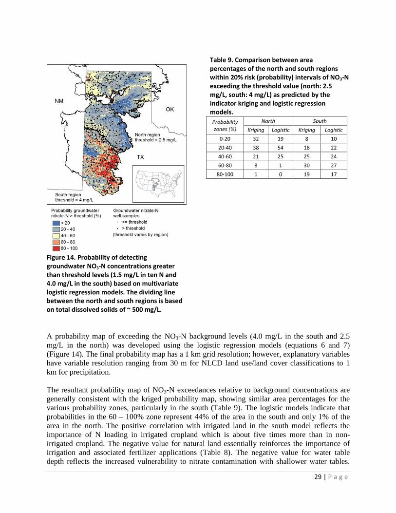
29 | P a g e
Figure 14. Probability of detecting groundwater NO3-N concentrations greater than threshold levels (1.5 mg/L in ten N and 4.0 mg/L in the south) based on multivariate logistic regression models. The dividing line between the north and south regions is based on total dissolved solids of ~ 500 mg/L.
Table 9. Comparison between area percentages of the north and south regions within 20% risk (probability) intervals of NO3-N exceeding the threshold value (north: 2.5 mg/L, south: 4 mg/L) as predicted by the indicator kriging and logistic regression models. Probability zones (%)
North South Kriging Logistic Kriging Logistic
0-20 32 19 8 10 20-40 38 54 18 22 40-60 21 25 25 24 60-80 8 1 30 27
80-100 1 0 19 17
A probability map of exceeding the NO3-N background levels (4.0 mg/L in the south and 2.5 mg/L in the north) was developed using the logistic regression models (equations 6 and 7) (Figure 14). The final probability map has a 1 km grid resolution; however, explanatory variables have variable resolution ranging from 30 m for NLCD land use/land cover classifications to 1 km for precipitation. The resultant probability map of NO3-N exceedances relative to background concentrations are generally consistent with the kriged probability map, showing similar area percentages for the various probability zones, particularly in the south (Table 9). The logistic models indicate that probabilities in the 60 – 100% zone represent 44% of the area in the south and only 1% of the area in the north. The positive correlation with irrigated land in the south model reflects the importance of N loading in irrigated cropland which is about five times more than in non-irrigated cropland. The negative value for natural land essentially reinforces the importance of irrigation and associated fertilizer applications (Table 8). The negative value for water table depth reflects the increased vulnerability to nitrate contamination with shallower water tables.

30 | P a g e
Clay content is important in the north region where soils vary from clay loam to sand. High groundwater nitrate levels in this area are essentially restricted to isolated pockets of sandy soils in the region. In the south region, soil texture is mostly coarse grained with little variability and as a result is not an influential factor. Inorganic fertilizers are also important in the north region and may be considered similar to N loading in irrigated land in the south model. In the northern region, precipitation is an important factor in the model due to the wider range of average annual precipitation received across the region (Figure 4). Water table depths are important in both regions but more important in the south because the water table is too deep for contamination in much of the north region. Therefore, the combination of fine grained soils and deep water tables in the north results in lower vulnerability to nitrate contamination than in the south where coarser grained soils, shallower water tables, and similar N loading lead to a much higher vulnerability to nitrate contamination. Land Use and Soil Texture Impacts on Unsaturated Zone Nitrogen Inventories Unsaturated zone profiles provide a link between the land surface and the underlying aquifer that can be used to further evaluate the controls on groundwater nitrate contamination identified through logistic regression. A cross plot of unsaturated zone NO3-N versus Cl inventories, normalized by profile depth, shows distinct grouping related to land use and soil texture (Figure 15, Tables 1-3). Natural ecosystem (grassland/rangeland) profiles generally have high Cl and low NO3-N inventories whereas rainfed agroecosystems generally have the opposite; low Cl and moderate to high NO3-N inventories. Profiles under irrigated agroecosystems generally have high Cl and high NO3-N inventories. The comparison is complicated because vertical variations in land use are also recorded in profiles that have transitioned from natural ecosystems, to rainfed cropland, and sometimes to irrigated cropland. Deeper sections of rainfed profiles may reflect natural ecosystems where profile depths are sufficiently deep.
Figure 15. Relationship between chloride and nitrate-N inventories normalized by depth for boreholes in different landuse (indicated by symbol shape) and soil texture settings (indicated symbol color fill shade). Large symbols indicate category mean values. Natural: squares, Rainfed: circles, Irrigated: triangles, Coarse grained soils: lighter shades, Fine grained soils: darker shades. With the exception of profiles in coarse textured soils in the north region, high Cl in native grassland/rangeland profiles (median 964 kg/ha/m) is attributed to little or no

31 | P a g e
percolation/recharge in many of these profiles. The general lack of recharge is attributed to perennial vegetation (grasses and shrubs) scavenging all the infiltrated water entering the profile since Pleistocene times some 10,000 yr ago (Scanlon et al., 2005). Plants transpire water leaving Cl in the soil profile to accumulate over millennial timescales. Generally low NO3-N in these profiles (median 5.0 kg/ha/m) has been attributed to accumulation of N from atmospheric deposition mostly as SON rather than as nitrate (NO3-N) (Scanlon et al., 2008, 2010a). Soil texture also plays a role as shown by fine textured soils (median clay 27%) under native grassland having higher Cl (median 1,350 kg/ha/m) but lower NO3-N (median 4.0) than coarser textured soils within the same land use (median clay 16%, Cl 23 kg/ha/m; NO3-N 10 kg/ha/m). The transition from native grassland/rangeland to rainfed cropland did not impact Cl profiles in fine grained soils (median clay content 42%; median Cl inventory 826 kg/ha/m), mostly in the north region; however, NO3-N inventories in these profiles (34 kg/ha/m) are much higher than those under natural vegetation in this region and may be related to mineralization/nitrification of SON. In coarser textured soils, cultivation in the early 1900’s generally increased percolation that is attributed to crops with short growing seasons and winter and summer fallow periods, allowing infiltrated water to percolate through the soil profile. The modified hydrology of these systems generally flushed Cl that accumulated under native vegetation resulting in Cl inventories (median 11 kg/ha/m) almost two orders of magnitude lower than similar native grassland sites. The changed hydrology also facilitated mineralization of SON thus increasing NO3 inventories by about an order of magnitude (median 39 kg/ha/m) relative to those under native vegetation. About half of the profiles under rainfed agroecosystems are partially flushed, rather than fully flushed (not plotted in Figure 15). These sites have higher Cl inventories below the flushed zone (median 523 kg/ha/m) because of incomplete flushing and NO3-N inventories (92 mg/ha/m) are much higher than those under fully flushed profiles. Irrigated profiles generally have high Cl inventories (median 1264 kg/ha/m) that are similar to those under natural grassland/rangeland ecosystems (883 kg/ha/m). The Cl inventories in irrigated profiles depend in part on the Cl concentration in the irrigation water. Lower Cl inventories in some irrigated profiles reflect low Cl concentrations in irrigation water. Irrigated profiles also have high NO3-N inventories (132 kg/ha/m) because of higher N fertilizer amendments associated with greater projected irrigated crop yields and NO3-N in irrigation water (roughly 10 – 20% of total). Similarly, finer textured profiles (median clay 42%) under irrigated cropland have higher Cl (1264 vs 740 kg/ha/m) than coarser textured profiles (median clay 26%) but similar NO3-N (132 vs 127 kg/ha/m). Evaluation of Sources of Nitrate Potential sources of NO3-N include atmospheric deposition, fertilizers (organic and inorganic), irrigation water, mineralization and nitrification of SON, biological N fixation, and septic leach field effluent. N fixation is not considered an important source because the native vegetation or major crops grown in the THP are not N fixers. Although quantitative estimates of atmospheric deposition are low (1.3 – 7.0 kg N/ha/yr), it is most likely the only nitrate source in natural ecosystems and, like Cl, may have been accumulating over the past 10,000 – 15,000 yr. N can accumulate as SON or as NO3-N. Profiles under natural ecosystems generally have low NO3-N (Figure 15) and most N accumulates as SON, which is high. Fine-textured soils have a greater capacity to physico-chemically protect organic matter compared with coarse textured soils and

32 | P a g e
therefore N inputs favor more accumulation as SON (Baer et al., 2010). Soil organic carbon (SOC) is also high in natural ecosystem profiles (Figure 16). Previous studies in the SHP indicate that mineralization and nitrification of SON was important based on the presence of high NO3-N inventories in deeper parts of the profiles corresponding to pre-cultivation based on chloride mass balance ages of soil water (Scanlon et al., 2008). Fertilizers are an obvious source of N and may explain high N levels, particularly under irrigated cropland. Higher NO3-N in domestic wells relative to irrigation wells suggests that septic leach fields may provide an important local source of NO3-N in groundwater in these regions.
Figure 16. Relationship between total N and total C in the 0-0.6 m depth interval for selected borehole profiles. Mineralization and Nitrification of Soil Organic Nitrogen Previous studies showed that the major source of increased NO3–N in rainfed cultivated profiles, unflushed Cl profiles and deeper sections of partially flushed Cl profiles is mineralization and nitrification of SON. In the shallower, flushed section, NO3-N sources may be derived from mineralization of SON and fertilizer application. The previous analysis of these sources focused on the SHP and this work extends the analysis to the CHP. The results are similar in both regions and show that old (pre-cultivation) soil water, dated using the chloride mass balance approach (Scanlon et al., 2008) has high NO3-N inventories (median 242 kg/ha). These NO3-N inventories account for 86% (median) of the total NO3-N in these profiles. Previous studies showed that N and O isotopes of NO3 support mineralization and nitrification of SON (Scanlon et al., 2008). Wetter conditions in this zone based on soil matric potential measurements may have caused increased microbial activity that accounted for mineralization in this deeper zone associated with land use change from native vegetation to cropland. In this study we also quantified SON and SOC in the shallow subsurface (0.6 m zone) from 12 profiles under different land uses. Results show that SON and SOC are highest under natural ecosystems (rangeland) and lowest under rainfed (non-irrigated cropland) ecosystems (Figure 16). Values in irrigated areas generally fall between natural and rainfed areas. SON and SOC values may also vary with soil texture and comparisons of the impacts of land use should be made using adjacent profiles with similar soil textures. These comparisons are consistent with the regional analysis, confirming that SOC and SON are highest under natural ecosystems and lowest under rainfed cropland and in-between for irrigated profiles. These profiles also show lower SOC and SON levels in coarser textured profiles (Figure 16).

33 | P a g e
Nitrogen Balance in Unfertilized Rainfed Cropland Region Unsaturated profiles with a non-fertilized cultivated cropland land use and detailed crop production records since 1937 (described earlier) as well as adjacent profiles under natural ecosystems provide a unique opportunity to quantify mineralization and nitrification of SON (Figure 17). The total N inventory under native vegetation is 9,314 kg/ha (upper 0.6 m) whereas that under adjacent unfertilized cropland is 7,123 kg/ha (Table 10, Figure 18). The reduction in total N is attributed to mineralization and nitrification of SON. Most (~80%) of this mineralized-nitrified SON can be accounted for in harvested crops (wheat and grain sorghum), which totaled 1,730 kg/ha (Figure 19). Inventories of NO3-N in the deeper profile (0.6 – 14.5 m) totaled 220 kg/ha and is attributed to leaching of NO3-N from the shallow subsurface. This N balance analysis provides strong evidence for mineralization and nitrification of SON in this region. Table 10. N balance for rainfed cultivated plots in Bushland, 1927-2012 Source/Sink kg/ha Total N inventory of native rangeland in 1927 (0 – 0.6 m)a 9314 Export of crop N 1927 - 2012 (wheat and sorghum grain)b -1730 Fertilizer N 0 Mean increase in borehole NO3
− + NO2− from native rangeland surfaces to present day cultivation (0.6 – 14.5 m) -220
Total N inventory of dryland cultivated systems 2012 (0 – 0.6 m) -7123 Balancec 241 90% Confidence interval ±139 a Atmospheric deposition (~2.34 kg ha-1 yr-1) is not included in the balance because this quantity cancels out assuming that present day N inventory on rangeland includes 86 years of accumulation equivalent to that received on the dryland cultivated systems. b In years when crop yields were not available (29 of 86 years for wheat and 7 of 64 years for sorghum), grain yield was estimated based on county and state records weighted according to factors determined from yield ratios with Bushland in years with data. Total N in wheat and sorghum was calculated as 2.30 and 1.87 percent of dry grain weight, respectively. c Change in bulk density was not considered in this calculation because differences between native rangeland and dryland cultivated soil were insignificant (0.02 Mg m-3). Assuming SOC and SON mineralization rates can be described by exponential decay (Lamb et al., 1985) with a rate constant obtained from the current rainfed cultivated and initial native grassland N inventories, ~50% of the mineralization of SON occurred prior to 1941. This analysis indicates that N exported in the grain began to exceed N mineralization rates in 1978 and that currently, the N export rate exceeds the mineralization rate (23 kg/ha/yr) by 14 kg/ha/yr (Figure 19). Wheat, and to a lesser extent sorghum, is likely assimilating additional N from NO3–N in the 1 – 2 m zone in the soil profile which was largely mineralized in the mid-1900’s. Earlier values of mineralization rates of 50 kg/ha/yr for these plots (Eck and Jones, 1992) seem greatly overestimated because this would require a more than doubling of total soil N from initiation of cultivation to present day inventories as determined in this study (Table 10). Eventually, accessible NO3–N sources will decline with time due to assimilation by the crops and continued leaching below the root zone. Presently, rainfed crops on no tillage plots may require supplemental N fertilizer because, unlike stubble-mulch plots, most of the NO3–N inventory is below 3 m depth.

34 | P a g e
Figure 17. Profiles of water-extractable chloride and nitrate+nitrite-N in a) natural (borehole POT07-04), b) rainfed (borehole POT08-06), and c) irrigated (borehole POT08-02) settings in fine grained (Pullman Clay Loam) soils.
Figure 18. Profiles of average a) total N and b) total C concentrations in the 0 – 0.6 m depth interval for profiles under natural, rainfed, and irrigated settings in fine grained (Pullman Clay Loam) soils. Natural profiles represent averages of samples from boreholes POT07-04 and POTEXC. Rainfed profiles represent averages of samples from boreholes POT06-02 and POT08-06. Irrigated profiles represent averages of samples from boreholes POT08-02, POT08-03, and POT08-09.
Figure 19. Annual rates of N exported in harvested crops and minearalization of organic N based on detailed records at Bushland.

35 | P a g e
Stable Isotopes Stable isotopes (δ15N) are of limited value in distinguishing different NO3-N sources because, as noted in Scanlon et al., 2008; NO3-N from SON and from fertilizers undergoes similar processes (mineralization and nitrification) because the dominant fertilizer source is NH3 (Table 5). The δ15N profiles seem to reflect the degree of disturbance with low δ15N near the surface (5.1 – 6.3‰) and greater stratification with depth under the native grassland as a result of accumulation of 15N-depleted plant residues near the surface (Högberg, 1997). In the Potter county sites, δ15N at 0 – 0.05 m was 5.4, 6.4, and 8.7‰ for native grassland, cultivated rainfed, and irrigated plots, respectively. Additionally, the change in δ15N from 0 to 0.15 m in these plots was 0.24, 0.13 and -.13 ‰ per m respectively which likely reflects the stratification of δ15N under native grasslands and homogenization of profiles under tillage. The δ13C isotopes of the SOC were analyzed to assess impacts of the shift from natural to cultivated ecosystems on the relative proportions of SOC derived from the native vegetation versus the cropping system. The δ13C isotopes should reflect that of the original vegetation. Native grasses have a C4 photosynthetic pathway with typical δ13C values ranging from -17‰ to -9‰ (mean ~ -13‰) while wheat and cotton have a C3 photosynthetic pathway with typical δ13C values of -32‰ to -22‰ (mean -27‰) (Boutton et al., 1998). Corn and sorghum are C4 plants, similar to native grasses, which complicate the analysis. Most profiles show increasing δ13C with depth, particularly in the upper 0.1 to 0.2 m depth zone, attributed to increasing fraction of organic carbon formed from input of native C4 plants with depth. Implications for Nitrate Management Nitrogen management in terms of environmental impacts should focus in the south region where nitrate contamination is highest as a result of coarse textured soils and shallow water tables. Regardless of source, this area has the highest vulnerability to nitrate contamination and should be the focus area of planned management efforts. Various approaches can be used to reduce groundwater N contamination, including reducing N fertilizer application rates by taking credit for (a) residual N in soils and (b) N in irrigation water. Residual soil NO3-N in the upper 0.6 m of the SHP is high and was estimated to be 27 kg/ha (Bronson et al., 2011). Producers should be sampling deeper than 0.15 to 0.2 m (standard), perhaps down to 0.6 m, to evaluate the total mineralized nitrogen available (NO3) to the crop and include this information in estimating the fertilizer rate (Bronson et al., 2009; Halvorsen et al., 2005; Appendix A). Under irrigated conditions (e.g. corn) residual N may be available to the next crop; however, if another corn or shallow rooted crop is grown, this NO3 may be leached below the root zone of corn (1 m) prior to the time roots penetrate this deep (i.e. pre-irrigation of 3 inches is not uncommon). Under these circumstances, a winter cereal crop planted after corn harvest may be useful for scavenging residual N deep in the profile (Shipley et al. 1992). This might be considered by operators in the near future because groundwater pumping limits in the High Plains Underground Water District will be reduced to 15 inches/year – insufficient (or too risky) for annual corn production (corn could still be grown every other year). Nitrate inputs from septic tanks and landscape fertilization should also be considered when thinking about nitrate reduction in the area. Properly locating septic systems relative to domestic

36 | P a g e
wells and ensuring that the leach field will function properly are musts when reducing potential nitrate contamination from septic systems. Landscape fertilization could also constitute a significant localized source of nitrate input to underlying aquifers. In this part of the state, irrigation is required to keep lawns growing year round and could easily enhance nutrient leaching into the aquifer over time. As a result, nutrient and irrigation application timing and rates should be managed closely to reduce nitrate leaching potential. Previous analyses for the SHP suggest that N in irrigation water represents ~ 15% of required N application for cotton, based on a projected yield goal of 1,400 kg lint/ha with a N requirement of ~ 140 kg N/ha (Bronson et al., 2011; Yabaji et al., 2009). The N credit for irrigation was based on 11 inches of in-season irrigation with 8 mg/L NO3-N in irrigation water. A N calculator was developed to estimate the fertilizer application required for center pivot and subsurface drip irrigation (SDI) systems in the SHP (http://soiltesting.tamu.edu/cottonNcalc/cottonNcalc.htm) that takes credit for residual N in the soil profile and N in irrigation water for irrigated cotton (Appendix A). The approach of crediting NO3-N in groundwater-fed irrigation is also recommended in the Central Valley of California and has been termed “pump and fertilize” (Harter et al., 2012). Appropriate timing of N fertilizer application is also important to reduce N leaching as a premature application can allow N to leach below the root zone before it is utilized. Fall applications of N are also used in some areas; however, these are not recommended unless fall cover crops are planted. The actual rate of N fertilizer applied should depend on the soil test N and the yield response curve (for a particular crop/county/region) using past yield records vs. N rate. Use of cover crops is another approach to reduce N leaching into underlying aquifers. These are useful for scavenging for N (rye, alfalfa, wheat); however, cover crops are generally not considered an option in the THP because water is generally limiting. Conclusions Analysis of groundwater nitrate contamination in the THP based on 1,232 data points shows that nitrate contamination is highest in the southern region, coinciding with high total dissolved solids (TDS ≥500 mg/L), and much lower in the northern region with low TDS. Median nitrate concentration is 4.8 mg/L in the south, 250% higher than in the north (1.9 mg/L). Kriging shows the regional distribution of high nitrate contamination in the south associated with coarser grained soils (S: median clay content 24%; N 31%) and shallower water table depth (S: 26 m: N 62 m) relative to the north. Depth variations based on LOWESS analysis shows that background NO3-N concentrations in the south region is 4.0 mg/L and 2.5 mg/L in the north region. Multivariate logistic regression analysis of the probability of exceeding background NO3-N concentrations indicates that probabilities are higher where water tables are shallow and natural and irrigated land is prevalent in the south and probabilities are lower where soils are finer grained, N loading from inorganic fertilizers are higher, precipitation is lower, and water table is deeper in the north. Unsaturated zone NO3-N profiles link the land surface with underlying aquifers to assess

37 | P a g e
processes controlling groundwater NO3-N contamination. Nitrate inventories are low under native grassland/rangeland vegetation throughout the THP and coincide with high Cl inventories which indicate little or no recharge except were soils are very coarse grained in the north. Conversion from rangeland to cropland resulted in increases in NO3-N inventories in fine grained soils where Cl was not displaced yet also increased NO3-N in coarse grained soils where Cl is flushed through the profile. Much of the NO3-n in the deeper portion of the rainfed profiles is attributed to mineralization/nitrification of SON during initial cultivation. This is supported by profiles in rainfed cropland that had never been fertilized and showed that N in wheat/sorghum harvests could be explained by mineralization/nitrification of SON. Irrigated profiles in the THP are characterized by high N inventories and generally high Cl inventories attributed to Cl in irrigation water or evapoconcentration of irrigation water. Analysis of groundwater and unsaturated zone data provide a comprehensive understanding of groundwater NO3-N contamination, emphasizing land use, soil texture, and water table depth as the primary factors controlling NO3-N contamination. Groundwater vulnerability to contamination is highest in the south where soils are coarse, the water table is shallow, and N loading from mineralization/nitrification of SON is high. In contrast, groundwater vulnerability is low in the north region where soils are often fine grained and water table is generally deep. Future groundwater NO3-N contamination could be reduced by decreasing N application rates as a result of crediting N in irrigation water and residual N in soil profiles. The timing of N applications could also be improved to coincide with crop growth. The results of this study have important implications for managing groundwater NO3-N contamination and illustrate the ability to extract nitrogen from groundwater by deficit fertilizing to meet crop needs. Results also emphasize the importance of mineralization /nitrification of SON as an important N source in this region.

38 | P a g e
Impact of Well Water Nitrate on Crop Production and Residual Soil Nitrate The Seymour Aquifer has the highest median NO3 concentration among the nine major aquifers in Texas (13.5 mg NO3-N L-1, Hudak, 2000). Recent research has indicated that NO3 levels have persisted, and perhaps increased, over the last 40-50 years (Chaudhuri et al., 2012). As these levels exceed the EPA Safe Drinking Water Standards (10 mg NO3-N L-1), human health concerns usually receive the most attention. However, these elevated NO3-N levels could provide a benefit to producers of irrigated crop production. A two-year study in Colorado concluded that when properly used, NO3-N crediting is a sound economic and agronomic practice (Bauder and Waskom, 1999). Thus, our hypothesis is that accounting for well water NO3-N toward crop N requirements can reduce fertilizer N inputs and subsequently reduce residual soil NO3-N and the risk of NO3-N leaching. As fertilizer N inputs are reduced due to NO3-N crediting, substantial economic savings could also be realized by producers. Materials and Methods Demonstration trials were initiated during the 2010 growing season and repeated in 2011 and 2012 at the Texas A&M AgriLife Chillicothe Research Station (CRS) near Chillicothe, TX. Demonstrations at CRS targeted three different irrigation systems cropped to cotton: 1) SDI; 2) furrow; and 3) overhead sprinkler irrigation (Figure 20). The sprinkler system was a standard low elevation spray application (LESA) center-pivot system. The SDI systems consisted of drip tape approximately 30 cm below the soil surface with emitter spacing of 40 cm. Soil types varied for each irrigation system. The LESA demonstration site consisted of a Grandfield fine sandy loam (Fine-loamy, mixed, superactive, thermic Typic Haplustalfs); the SDI system on a Abilene clay loam (Fine, mixed, superactive, thermic Pachic Argiustolls); and the furrow irrigation was located on a Rowena clay loam (Fine, mixed, superactive, thermic Vertic Calciustolls). Within each irrigation system, five fertility management strategies were demonstrated, including:
1. Control (N from irrigation water only; no inorganic N fertilizer) 2. N applied based on soil testing and yield goal, disregarding NO3-N content in the well water
(uncredited N) 3. N and P application based on soil testing and yield goal disregarding NO3-N content in the well
water (uncredited N + P) 4. N application based on soil testing, yield goal and accounting for NO3-N in well water (Credited
N) 5. N and P application based on soil testing, yield goal, and accounting for NO3-N in well water
(Credited N + P) Fertility treatments were demonstrated three times within the furrow irrigation site and four times in the LESA and SDI systems. Annual yield goals were 1120 kg ha-1 for the furrow system and 1680 kg ha-1 for the LESA and SDI systems. Nitrogen needs were assumed to be 56 kg for every 560 kg of lint yield. Thus, annual crop N needs were 112 kg ha-1 for the furrow system and 168 kg ha-1 within LESA and SDI systems. The amount of N applied annually was based upon the yield goal N requirement minus the residual soil NO3-N in the top 0.6 m of the soil

39 | P a g e
profile. For credited N treatments, those treatments accounting for the NO3-N concentration in the well water, it was estimated that 30 cm of irrigation water would be applied annually. This amount is based upon historical irrigation requirements for cotton at CRS. We also knew that average well water NO3-N at CRS was 20 mg L-1. Hence, 30 cm irrigation water containing 20 mg NO3-N L-1 will provide 62 kg N ha-1 (Table 11). Thus, N application rates were reduced by 62 kg ha-1 in credited treatments. Treatments including P applications were based upon Mehlich III analysis of soil samples taken to a depth of 0.15 m. Liquid fertilizer was applied pre-plant over the entire demonstration area to achieve a uniform application and then incorporated by tillage. All plots were irrigated with a goal to achieve 100% ET replacement based on data obtained from the High Plains ET network. Water samples were collected weekly and analyzed for NO3-N to determine the amount of in-season N application supplied by well water. Prior to defoliation, cotton samples were clipped and dissected (burrs, stems, leaves, and seed) to determine N content and N uptake. All plant samples were dried and ground and analyzed for total N using combustion analysis. Defoliants were used as a harvest aid in all demonstration areas. All demonstration areas were mechanically harvested and processed to determine lint yields.
Figure 20. Irrigation demonstration areas at Chillicothe Research Station. Soil samples were taken to a depth of 0.9 m using a hydraulic Giddings probe and were segmented into depth increments of 0-0.15, 0.15-0.30, 0.30-0.45, 0.45-0.60, and 0.60-0.90 m. Soil samples were taken prior to planting in 2010, 2011, 2012 and after harvest in 2012. Samples were dried at 60oC and ground to pass a 2mm sieve. Soil NO3-N was determined colorimetrically after extracting 2 g soil with 20 mL KCl for 1 hr. Mehlich III P was also
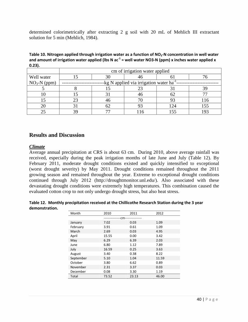
40 | P a g e
determined colorimetrically after extracting 2 g soil with 20 mL of Mehlich III extractant solution for 5 min (Mehlich, 1984). Table 10. Nitrogen applied through irrigation water as a function of NO3-N concentration in well water and amount of irrigation water applied (lbs N ac-1 = well water NO3-N (ppm) x inches water applied x 0.23). cm of irrigation water applied Well water NO3-N (ppm)
15 30 46 61 76 --------------------------kg N applied via irrigation water ha-1--------------------------
5 8 15 23 31 39 10 15 31 46 62 77 15 23 46 70 93 116 20 31 62 93 124 155 25 39 77 116 155 193
Results and Discussion Climate Average annual precipitation at CRS is about 63 cm. During 2010, above average rainfall was received, especially during the peak irrigation months of late June and July (Table 12). By February 2011, moderate drought conditions existed and quickly intensified to exceptional (worst drought severity) by May 2011. Drought conditions remained throughout the 2011 growing season and remained throughout the year. Extreme to exceptional drought conditions continued through July 2012 (http://droughtmonitor.unl.edu/). Also associated with these devastating drought conditions were extremely high temperatures. This combination caused the evaluated cotton crop to not only undergo drought stress, but also heat stress. Table 12. Monthly precipitation received at the Chillicothe Research Station during the 3 year demonstration.
Month 2010 2011 2012 ---------------cm--------------- January 7.02 0.03 1.09 February 3.91 0.61 1.09 March 2.69 0.03 4.95 April 15.55 0.00 3.42 May 6.29 6.39 2.03 June 6.80 1.12 7.89 July 16.59 0.25 3.63 August 3.40 0.38 8.22 September 5.10 1.04 11.59 October 3.80 6.62 0.89 November 2.31 3.37 0.03 December 0.08 3.30 1.19 Total 73.52 23.13 46.00

41 | P a g e
As expected, drought conditions resulted in greater irrigation demand. At CRS, annual irrigation needs for cotton (based upon historical records) is estimated to be 30 cm. Water applied via irrigation was below average during 2010 for all irrigation systems (Table 13). However, the amount of irrigation water applied was at least 128% and 25% greater than average in 2011 and 2012 respectively for LESA and SDI systems. The furrow irrigation system at Chillicothe Research Station is supplied from a sole well and cycled among several fields. Thus, “on demand” irrigation was not possible during the drought of 2011 and 2012. This resulted in lower irrigation amounts for the furrow system compared to the LESA and SDI systems (Table 13). Table 13. Annual amount of irrigation water applied to respective demonstrated irrigation systems at CRS.
Irrigation System 2010 2011 2012 -------------------------cm------------------------ Furrow 19.1 29.1 13.2 LESA 19.9 69.1 39.7 SDI 25.4 68.4 37.4
Subsurface Drip Irrigation Entering the 2010 growing season, residual soil NO3-N to a depth of 0.6 m was 22 kg ha-1 within the SDI demonstration area. Fertilizer N applications were adjusted accordingly (Table 14). In 2010, pre-plant fertilizer N applications were 146 kg ha-1 for uncredited treatments compared to 84 kg ha-1 for credited treatments (Table 14). Accounting for well water NO3-N resulted in a 42% reduction in applied N fertilizer. Treatments including P received 28 kg P ha-1 pre-plant in years 1 and 2 and 22 kg P ha-1 in year 3. Table 14. Nitrogen and phosphorus fertilizer application rates applied pre-plant for each year of the demonstration within the subsurface drip irrigation system.
Treatment Nitrogen Applied†
Phosphorus Applied
Nitrogen Applied
Phosphorus Applied
Nitrogen Applied
Phosphorus Applied
2010 2011 2012 ---------------------------kg ha-1------------------------- Control 0 0 0 0 0 0 Uncredited N 146 0 123 0 0 0 Uncredited N + P 146 28 123 28 0 22 Credited N 84 0 84 0 0 0 Credited N + P 84 28 73 28 0 22
†Nitrogen applied is equal to N needs for yield goal minus soil NO3-N in upper 0.6 m of the soil profile. Lint yields in 2010 ranged from 1133 to 1261 kg ha-1 (Figure 21A), which were 25-32% lower than our yield goal of 1680 kg ha-1. While all fertilizer treatments resulted in a numeric increase in yield over the control, there was little difference among treatments. This was somewhat surprising, as a greater response between the control and fertilized treatments were expected. As irrigation requirements were less than expected in 2010, the N applied through irrigation water

42 | P a g e
was 54.5 kg ha-1 (Figure 22). This was slightly lower than the 62 kg ha-1 estimated during pre-season calculations. Within the SDI system, an increase in lost bolls was noted late in the season due to uncertain factors. Excess N application can result in decreased boll retention and increased pest problems (Hons et al., 2004). This may partially explain the reason for no yield response of fertilized treatments over the unfertilized control. A better representation is evident through N uptake calculations, as cotton clippings were taken in late August, approximately 2 months prior to harvest and prior to noted loss of bolls. Nitrogen uptake calculations showed a response to N inputs (Figure 21B), as treatments receiving pre-plant N fertilizer resulted in greater N uptake compared with the control (Figure 21B). The most important observation during 2010 is the fact that there were no differences among uncredited and credited treatments for lint yield and N uptake. Thus, results in the initial year indicated that cotton was utilizing NO3-N in the irrigation water. Soil sampling prior to the 2011 cropping season indicated that residual soil NO3-N was greater for uncredited treatments than credited treatments (Figure 23). Pre-plant N applications were similar for credited treatments in 2010 and 2011 (Table 12), as soil NO3-N in the upper 30 cm of the soil profile was also similar between years (Figure 23). In contrast, pre-plant N requirements for uncredited treatments declined from 146 kg ha-1 in 2010 to 123 hg ha-1 in 2011 due to increasing residual soil NO3-N (Table 12; Figure 23).
Figure 21. A) Lint yield and B) nitrogen uptake from demonstration plots within the subsurface drip irrigation system at Chillicothe Research Station 2010-2012.
Figure 22. Nitrogen supplied by NO3-N in irrigation water for 2010-2012 growing seasons within the subsurface drip irrigation system.
Lint
Yie
ld (k
g ha
-1)
0
200
400
600
800
1000
1200
1400
1600
1800
Control Uncredited N Uncredited N + P Credited N Credited N + P
2010 2011 2012
Nitr
ogen
Upt
ake
(kg
ha-1
)
0
50
100
150
200
250
A
B2010 2011 2012
Irrig
atio
n N
itrog
en A
pplie
d (k
g ha
-1)
0
20
40
60
80
100
120
140
160
180

43 | P a g e
Lint yields in 2011 were once again similar among all treatments (Figure 21A) but were much lower in 2011 than other years as a result of extreme drought and heat. Exceptional drought conditions increased the irrigation demand to 68 cm (Table 11); more than a 2 fold increase over average requirements. As a result, 158 kg N ha-1 was supplied by the irrigation water alone surpassing the 73 to 123 kg N ha-1 needed to meet crop N requirements (Table 12). Since naturally occurring NO3-N in irrigation water met crop N requirements, excess N was inadvertently applied to both credited and uncredited treatments. This explains the lack of N response (yield and N uptake) among treatments in 2011 (Figure 21A and 21B). As a result, residual soil NO3-N levels increased dramatically post 2011 and remained elevated through 2012 (Figure 23). Soil NO3-N in the upper 0.6 m post 2011 growing season increased by more than 12 fold compared with post 2010 measurements. Credited and uncredited treatments had higher post 2011 soil NO3-N levels than the control. Within credited and uncredited treatments, soil NO3-N levels increase by at least 5 fold compared to the previous growing season (Figure 22). Soil NO3-N levels were slightly higher for uncredited treatments compared to credited treatments.
Figure 23. Residual soil nitrate in the upper 0.6 cm for each treatment demonstrated in the subsurface drip irrigation system prior to the 2010 growing season and after each subsequent growing season. Increased irrigation demands and decreased crop production in 2011 led to higher N applications, reduced N uptake, and greater residual soil NO3-N levels. As a result, crop N requirements (169 kg ha-1) entering the 2012 growing season were fully met for all treatments by residual soil NO3-N in the upper 0.6 m and precluded the need to apply pre-plant N in 2012 (Table 12). As expected, no differences among treatments were noted in regards to lint yield and N uptake (Figures 21A and 21B). Irrigation water supplied 69 kg N ha-1 during the 2012 growing season, which was very close to the estimated value of 62 kg N ha-1 (Figure 22). Residual soil NO3-N levels decreased following the 2012 growing season (Figure 23) since additional fertilizers were
Control
Uncredited N
Uncredited N + P
Credited N
Credited N + P
Soi
l Nitr
ate
(kg
ha-1
)
0
50
100
150
200
250
300Pre 2010 Post 2010 Post 2011 Post 2012

44 | P a g e
not applied. Soil samples collected after the 2012 growing season (post 2012) showed that soil NO3-N levels decreased by 30% for the control treatment and 35 to 42% for credited and uncredited treatments (Figure 23). It should be noted that the highest yields were obtained during 2012 when no commercial fertilizer was applied (Figure 21A) thus highlighting the need for soil testing to a depth of at least 0.6 m, which can provide valuable N to desired crops. Low Elevation Spray Application Pivot Irrigation (LESA) After accounting for residual soil NO3-N in the upper 0.6 m, 146 kg N ha-1 was applied pre-plant to uncredited treatments in 2010 (Table 13). As within the SDI system, pre-plant commercial N application rates were reduced by 42% in credited N treatments compared with uncredited N treatments (Table 15). Uncredited and credited N treatments (with and without P) resulted in increased lint yield over the control (Figure 24A). Treatments receiving commercial N resulted in at least a 31% increase in lint yield over the control. The control treatment received 44 kg N ha-1 via NO3-N in the irrigation water (Figure 25). Due to below average irrigation requirements, the estimated N contribution from irrigation water (62 kg ha-1) was not met. However, there were no marginal differences between uncredited and credited treatments with lint yields ranging from 1481 to 1566 kg ha-1 (Figure 24A). These results show that reducing commercial N application rates by 42% had no effect on lint yield, indicating that NO3-N in irrigation water was being utilized by the crop. Phosphorus application resulted in similar lint yields and N uptake than treatments not receiving P applications (Figures 24A and 24B). Table 15. Nitrogen and phosphorus fertilizer application rates applied pre-plant for each year of the demonstration within the low elevation spray application pivot irrigation system.
Nitrogen Applied†
Phosphorus Applied
Nitrogen Applied
Phosphorus Applied
Nitrogen Applied
Phosphorus Applied
2010 2011 2012 ---------------------------kg ha-1------------------------- Control 0 0 0 0 0 0 Uncredited N 146 0 146 0 90 0 Uncredited N + P 146 28 146 28 101 39 Credited N 84 0 90 0 39 0 Credited N + P 84 28 90 28 56 39
†Nitrogen applied is equal to N needs for yield goal minus soil NO3-N in upper 0.6 m of the soil profile. Post 2010 soil sampling indicated that residual soil NO3-N levels were similar to levels prior to the 2010 growing season (Figure 26). Hence, pre-plant commercial N applications in 2011 mirrored those in 2010 (Table 15). Lint yields on the LESA irrigated plots were lower in 2011 than other years due to adverse environmental conditions. Lint yields were similar among all treatments in 2011, ranging from 866 to 907 kg ha-1 (Figure 24A). This can be explained by the fact that 167 kg N ha-1 was applied through NO3-N in the irrigation water alone (Figure 25). Coupled with residual soil NO3-N levels, N supplied by irrigation water exceeded crop N requirements yielding a substantial excess of N applied in those treatments fertilized with commercial N. This was reflected in post 2011 soil sampling where residual soil NO3-N levels in the upper 0.6 m increased by at least 3 fold (Figure 26). The increase in residual soil NO3-N was not as dramatic within the LESA system as observed in the SDI system. This is due to

45 | P a g e
differences in soil type. The LESA system is on a sandy loam soil compared with a clay loam soil encompassing the SDI system. Thus, leaching is more prone within the more porous sandy soil of the LESA system. Furthermore, irrigation within the LESA system was applied once a week in 2011 compared with daily applications in the SDI system. For example, the amount of water applied in a single application using the LESA system is evenly distributed over a 7 day period within the SDI system. This is supported in the findings of Sij et al. (2008) who conducted trials within the Texas Rolling Plains and concluded that NO3-N leaching is approximately twice as likely under pivot irrigation as under SDI.
Figure 24. A) Lint yield and B) nitrogen uptake from demonstration plots within the low elevation spray application pivot irrigation system at Chillicothe Research Station 2010-2012.
Figure 25. Nitrogen supplied by NO3-N in irrigation water for 2010-2012 growing seasons within the low elevation spray application pivot irrigation system.
Due to increased residual soil NO3-N, pre-plant commercial N applications were reduced in 2012 as compared to 2011 (Table 15). Credited N treatments resulted in 38 to 61% lower pre-plant commercial N applications compared with uncredited treatments. Lint yields were about 8% higher for uncredited N and credited N treatments compared with the control (Figure 24A). An even greater response was observed for treatments receiving P. Both uncredited N + P and credited N + P treatments increased lint yields by 18% over the control (Figure 24A). Soil test P levels were lower in post 2011, resulting in greater P application requirements in 2012 than any other year. This suggests that adequate P fertility likely aided proper plant N utilization. Nitrogen uptake was greater for fertilized treatments compared to the control, but was inconsistent among
Lint
Yie
ld (k
g ha
-1)
0
200
400
600
800
1000
1200
1400
1600
1800
2000
Control Uncredtied N Uncredited N + P Credited N Credited N + P
2010 2011 2012
Nitr
ogen
Upt
ake
(kg
ha-1
)
0
50
100
150
200
250
300
A
B2010 2011 2012
Irrig
atio
n N
itrog
en A
pplie
d (k
g ha
-1)
0
20
40
60
80
100
120
140
160
180

46 | P a g e
fertilized treatments (Figure 24B). Residual soil NO3-N treatments following the 2012 growing season remained the same or decreased for 4 of 5 treatments. With lower irrigation demand in 2012 as well as two irrigation applications weekly rather than one, leaching potential may have been lower during the 2012 season than the 2011 season.
Figure 26. Residual soil nitrate in the upper 0.6 m for each treatment demonstrated in the low elevation spray application pivot irrigation system prior to the 2010 growing season and after each subsequent growing season. Furrow Irrigation Pre-plant commercial N application rates in 2010 were 73% lower for credited N treatments than in uncredited N treatments (Table 16). Lint yields were 11 to 12% higher for all fertilized treatments compared with the control (Figure 27A). The exception was the uncredited N + P treatment, which resulted in a 6% lint yield increase over the control. Yield goals were exceeded in all credited and uncredited treatments. A treatment response for N uptake, with all credited and uncredited treatments occurred resulting in greater N uptake as compared to the control. Similar to the other irrigation systems, lint yields were not reduced with a significant decrease in pre-plant commercial N application. Residual soil NO3-N in the upper 0.6 m remained relatively constant from 2010 to 2011, resulting in similar pre-plant N application rates in 2011. Drought conditions had the greatest effect in the furrow demonstration area. Unlike pivot and SDI irrigation systems, uniform pre-water or post-plant applications for stand establishment are not as easily achieved. For this demonstration, pre-watering was not conducted. Furrow irrigation at CRS is rotated among several fields which limited watering during the demonstration to about every two weeks. Due to exceptional drought and heat conditions, plant establishment was fair. The furrow irrigation
Control
Uncredited N
Uncredited N + P
Credited N
Credited N + P
Soi
l Nitr
ate
(kg
ha-1
)
10
20
30
40
50
60
70
80
90
Pre 2010 Post 2010 Post 2011 Post 2012

47 | P a g e
system could not keep up with water demand resulting in only 29 cm of the 70 cm water demand being applied. Under normal farming operations, the cotton crop would have been declared a failure; however, lint yields and N uptake were measured for evaluation purposes. Table 16. Nitrogen and phosphorus fertilizer application rates applied pre-plant for each year of the demonstration within the furrow irrigation system.
Nitrogen Applied†
Phosphorus Applied
Nitrogen Applied
Phosphorus Applied
Nitrogen Applied
Phosphorus Applied
---------------------------kg ha-1------------------------- 2010 2011 2012 Control 0 0 0 0 0 0 Uncredited N 84 0 78 0 11 0 Uncredited N + P 84 28 67 28 11 29 Credited N 22 0 9 0 0 0 Credited N + P 22 28 22 28 0 29
†Nitrogen applied is equal to N needs for yield goal minus soil NO3-N in upper 0.6 m of the soil profile. As expected, residual soil NO3-N after the 2011 growing season increased by at least 2 fold (Figure 29). No pre-plant commercial N applications were applied to the credited treatments and only 11 kg N ha-1 were applied to uncredited treatments (Table 16). Early in 2012, herbicide drift heavily damaged seedling cotton, resulting in poor stand establishment and survival. The demonstration area was harvested and N uptake was determined, with little response among treatments (Figure 27A and B). As within the SDI system, residual soil NO3-N was sufficient to meet crop requirements. Unlike the SDI and LESA systems, residual soil NO3-N increased after the 2012 growing season (Figure 29). Due to poor stand establishment, N uptake was probably overestimated. In cases where large “skips” occurred within the row, soil NO3-N values would be expected to be higher. Although care was taken to avoid these areas during soil sampling, high variance was possible due to the nature of the irrigation system and ambient environmental conditions. Under normal conditions, nitrate crediting is a sound practice within a furrow irrigation system. However, it is probably the most variable system and most difficult to predict. Economic Considerations We demonstrated that commercial N application rates can be reduced significantly as a result of accounting for well water NO3-N. Commercial N prices have increased 300% over the last decade. At CRS, the average NO3-N concentration in groundwater is 20 mg L-1 and based upon the historical average irrigation application, 30 cm of water is applied annually to cotton supplying 62 kg N ha-1. Commercial N prices were as high as $1.74 kg-1 N during this demonstration. Thus, the value of N in 30 cm of irrigation water at CRS is $107.88 ha-1 and shows that nitrate crediting can provide substantial cost savings if implemented. This is further exacerbated in drought years. As much as 69 cm water was applied in 2011, which provided N valued at $243.79 ha-1. Not only should the value of NO3-N in irrigation water be considered, but also residual soil NO3-N. After drought conditions or poor crop conditions, residual soil NO3-N was sufficient to supply 100% of crop N needs.

48 | P a g e
Figure 27. A) Lint yield and B) nitrogen uptake from demonstration plots within the furrow irrigation system at Chillicothe Research Station 2010-2012.
Figure 28. Nitrogen supplied by NO3-N in irrigation water for 2010-2012 growing seasons within the furrow irrigation system.
Well Water Example: After submitting a well water sample, a farmer finds the irrigation well water NO3-N content to be 13.5 mg L-1 (or ppm), which is the median NO3-N concentration in the Seymour Aquifer. The farmer’s historical records indicate that 30 cm (12 inches) of irrigation water is typically applied. The resulting N applied through irrigation water would be:
13.5 ppm NO3-N x 12 inches x 0.23 = 37 lb ac-1(42 kg ha-1). Assuming the price per pound of N fertilizer to be $0.60, the approximate cash value per pound of actual NO3-N per acre is $22.20. If the farmer is irrigating 120 ac, potential savings would be: $0.60 per lb N x 37 lb N ac-1 x 120 ac = $2,264 ($46.50 ha-1)
Lint
Yie
ld (k
g ha
-1)
0
200
400
600
800
1000
1200
1400
Control Uncredited N Uncredited N + P Credited N Credited N + P
2010 2011 2012
Nitr
ogen
Upt
ake
(kg
ha-1
)
0
50
100
150
200
A
B2010 2011 2012
Irrig
atio
n N
itrog
en A
pplie
d (k
g ha
-1)
0
20
40
60
80

49 | P a g e
Figure 29. Residual soil nitrate in the upper 30 cm for each treatment demonstrated in the furrow irrigation system prior to the 2010 growing season and after each subsequent growing season. Residual Soil Nitrate Example: A producer submits two composite soil samples, 0-6 in and 6-24 in (0-0.15 m and 0.15-0.6 m). Soil analysis indicates residual soil NO3-N to be 20 lb ac-1 in the upper 6 in (22 kg ha-1 in upper 0.15 m) and 15 lb ac-1 at the 6-24 in depth (17 kg ha-1 at 0.15-0.6 m). Thus, a total of 35 lb NO3-N ac-1 (39 kg ha-1) is available in the upper 24 in (0.6 m) of the soil profile. Potential savings due to soil testing over the 120 ac field is: $0.60 per lb N x 35 lb ac-1 x 120 ac = $2,520 ($21 ac-1 or $51.85 ha-1) The additions of soil testing to a depth of 24 in (0.6 m), rather than the typical 6 in (0.15 m) provided an additional 15 lb NO3-N ac-1 savings as well: $0.60 per lb N x 15 lb ac-1 x 120 ac = $1,080 ($9 ac-1 or $22.22 ha-1) Combining Soil and Water Testing: If the farmer implemented both well water testing and soil testing to a depth of 24 in (0.6 m), substantial savings would be realized. For the 120 ac field irrigation scenario described above, total savings would be: Soil Nitrate Value: $2,520 Water Nitrate Value: $2,260 Total Savings: $4,780 ($39.83 ac-1 or $98.35 ha-1)
Control
Uncredited N
Uncredited N + P
Credited N
Credited N + P
Soi
l Nitr
ate
(kg
ha-1
)
0
50
100
150
200
250
300
350
Pre 2010 Post 2010 Post 2011 Post 2012

50 | P a g e
Hons et al. (2004) showed that sampling soil to a depth of 0.6 m, as compared to 0.15 m, reduced recommended N application amount for a 2 bales of lint per acre yield goal by an average of about 30 percent. Obviously, savings per unit land area increases with increasing soil testing depth and well water testing. As seen in Table 10, N contributions from irrigation water increase dramatically with either increasing irrigation application rates or increasing NO3-N concentration. A cotton N calculator (http://soiltesting.tamu.edu/cottonNcalc/cottonNcalc.htm) was developed to aid farmers in determining potential N contributions from soil and water, based on inputted yield goal, soil NO3-N results at sampled depths, and water testing results (Appendix A). Soil and water testing is a relatively cheap investment considering the potential returns this work has examined and provided. For example, through the Texas A&M AgriLife Extension Soil, Forage and Water Testing Laboratory, cost of a routine soil test is $10 per sample ($20 for 0.15 m plus 0.15 to 0.6 m) and a routine water test is $20. As measured in this demonstration study and previous studies, NO3-N concentrations in well water have been shown to remain relatively constant over the course of the irrigation season. Hence, a single water sample prior to initiating crop irrigation should suffice to determine potential N contributions from well water. Conclusions In this demonstration, N applications were significantly reduced when accounting for well water NO3-N toward crop N needs without reducing lint yields within three different irrigation systems. During the 2011 drought, when yields were well below estimated yield goals and irrigation requirements were greater than expected, NO3-N in the well water supplied 100% of the crop N needs in SDI and LESA irrigation systems. As a result, there were no differences in lint yield among treatments and residual soil NO3-N levels increased. For cases in which yield goals are not achieved and/or elevated NO3-N in well water is not accounted for, NO3-N levels in the soil can rapidly buildup or leach through the profile. This increase was more dramatic in clay loam soils within SDI than sandy loam soils within the pivot system. Leaching of NO3-N is more likely in course textured soils and could be impacted by irrigation application method. Wells should be sampled every year prior to the growing season along with soil samples collected to a depth of at least 0.6 m and measured for NO3-N. Crediting well water NO3 toward crop N requirements can provide substantial savings in fertilizer costs and reduce the risk of leaching without compromising crop yields. To most effectively manage nitrogen to improve crop yield, economic profitability, and environmental sustainability, the following guidelines should be followed: • Determine a realistic yield goal • Collect and submit water samples for nitrate content from each well used for irrigation • Soil test for residual nitrate to a depth of 0.6 m (24 inches) every year Standard water testing ($20 per sample) and soil testing ($10 per sample) submittal forms can be found at the Texas A&M AgriLife Extension Soil, Water and Forage Testing Laboratory website (http://soiltesting.tamu.edu/). There are also numerous other commercial laboratories available for soil and water testing. While this demonstration focused on cotton, nitrate crediting should be a sound agronomic, economic, and environmental practice in other cropping systems as well. Further nitrate crediting demonstrations in additional cropping systems are warranted.

51 | P a g e
Education and Outreach A critical component of this project was conveying information to the general public through education and outreach through a variety of platforms to reach a diverse audience. To accomplish this objective and convey findings that will promote adoption of improved management practices by producers, fact sheets were produced, newsletter articles and news releases were distributed, a field day highlighting demonstration results was held and numerous presentations were given at local, regional, state and national meetings and conferences. Fact Sheets A factsheet entitled “Nitrates in Irrigation Water: An Asset for Crop Production” (DeLaune & Trostle, 2012) was developed and has been distributed widely a crop production programs across the THP and Rolling Plains regions of the state (Appendix A). This resource clearly and concisely describes nitrogen content common in irrigation water across the state, discusses federal drinking water standards and human health related to nitrate consumption, estimating nitrate application through irrigation water, potential cost savings to the producer as well as a few key considerations that producers should make when crediting their nitrate in irrigation water or soils. This fact sheet was published by the Texas A&M AgriLife Extension Service and is available for free on line at: http://www.agrilifebookstore.org/product-p/e-619.htm. Newsletters & News Releases Broad distribution of information related to this project and its findings was achieved through the inclusion of project findings in regional newsletters and statewide news releases. Two installments of the Buck Creek Watershed Partnership newsletter discussed nitrogen crediting and project findings as well as provided a recap of the Rolling Plains Summer Crops Field Day (Appendix A). These newsletters have a good distribution in Childress, Collingsworth and Donley counties but also make it to many other areas of the THP and Rolling Plains. Two news releases also highlighted the accomplishments of the project and promoted the Rolling Plains Summer Crops Field Day held at the Chillicothe Research Station near Chillicothe, TX on July 17, 2012 (Appendix A). These articles were released through AgriLife Today, Texas A&M AgriLife’s news outlet which has statewide exposure. Field Day The Rolling Plains Summer Crops Field Day was held in Chillicothe on July 17, 2012 and was attended by about 75 area producers, crop advisors and natural resource professionals. Attendees received a variety of information built around the central message of maximizing nutrient and water use efficiency. Specific topics discussed included irrigation scheduling technologies, optimizing fertilizer applications, no-till and cover cropping methods, soil health and fertility, and nitrate availability and crediting. Meetings & Conferences The presentation of project findings at local, regional, statewide and national meetings was the most effective means for distributing project findings to broad audiences. Meetings where

52 | P a g e
findings were presented included local programs such as the Texas Well Owner Network program held in Wellington, TX, regional events such as the Panhandle Peanut Growers Association Meeting held in Quail, TX and national programs like the Beltwide Cotton Conference Meetings held in Atlanta, GA and San Antonio, TX. Table 17 lists the meetings or conferences presented at, the event location and the approximate number of event participants. Additionally, three graduate student posters were presented with the posters taking two second places and one third place. Table 17. Meetings and conferences where project findings were presented Meeting/Conference Name Event Location Number
Attending AgriLife Administration Field Day Chillicothe Research Station 15 Beltwide Cotton Conference Atlanta, GA 35 Beltwide Cotton Conference Orlando, FL 45 Peanut Growers Association Quail, TX 30 Red River Basin Advisory Committee Amarillo & Wichita Falls, TX 65 Rolling Plains Summer Crops Field Day Chillicothe, TX 75 TSSWCB Board Meeting Temple, TX 40 American Society of Agronomy, Crop Science of America, Soil Society of America Tri- Society Meeting
Cincinnati, OH 35
Beltwide Cotton Conference San Antonio, TX 55 North Rolling Plains Ag Conference Vernon, TX 45 American Society of Agronomy Orlando, FL 30 Texas Well Owners Network Training Wellington, TX 15 Texas Well Owners Network Training Haskell, TX 25 Plant Protection Conference Bryan, TX 20

53 | P a g e
Project Conclusions The analysis of available groundwater nitrate levels as well as nitrates and chlorides in soil profiles in the THP and Rolling Plains confirm that nitrate is widely distributed at levels that are often in excess of EPA’s 10 mg/L MCL and that they are derived from a variety of sources. While this does pose a concern for public water supplies, this is a potential resource for farmers who irrigate their crops. In fact, through the judicious accounting of nitrates in soils and groundwater in meeting crop requirements, farms may actually be able to remediate aquifers. Nitrate concentrations were found to be highest in the southern region of the THP and are often associated with high total dissolved solids in excess of 500 mg/L. The regional distribution of high nitrate contamination in the south is often associated with coarser grained soils than exhibited in the north. Shallower water table depths in the south also tend to make this area more vulnerable to nitrate contamination than the north. To better understand the link between aquifers and the land above, nitrate in the unsaturated soil zone were evaluated. Profiles under native grassland/rangeland vegetation showed low nitrate levels that coinciding with high Cl levels that indicate little or no recharge except on very coarse grained soils. Cropped lands that are not irrigated show increases in NO3-N in fine grained soils where Cl was not displaced and also increased NO3-N in coarse grained soils where Cl is flushed through the profile. Much of the NO3-N in the deeper portion of these rainfed systems is attributed to mineralization/nitrification of soil organic nitrogen (SON). This SON was released into the profile when virgin prairies were initially cultivated in the late 1800s and early 1900s. Irrigated cropland profiles are also characterized by high nitrate inventories and generally high Cl inventories attributed to Cl in irrigation water or evapoconcentration of irrigation water. Collectively, these results illustrate that nitrates present in both soil profiles and underlying groundwater come from both natural and manmade sources. Analysis of groundwater and unsaturated zone data also provide a comprehensive understanding of groundwater NO3-N contamination pathways and the influences that land use, soil texture, and water table depth have on controlling NO3-N contamination. Groundwater vulnerability to contamination is highest in the south where soils are coarse and water table is shallow and N loading from mineralization/nitrification of SON is high. In contrast, groundwater vulnerability is lower in the north region where soils are often fine grained and water tables are generally deep. Overlying landuses and land management practices do influence the presence and quantity of nitrates found both in the soil and groundwater; however, soil types and the depth to water are the strongest factors controlling potential nitrate contamination of underlying groundwater. These findings suggest that future groundwater NO3-N contamination could be reduced by decreasing inorganic nitrate application rates and accounting for N in irrigation water and in soil profiles. Cropping demonstrations employing nitrogen crediting under various irrigation systems proved that nitrogen applications can be significantly reduced when accounting for well water NO3-N toward crop nitrogen needs without reducing lint yields. Additionally, residual soil nitrate levels also declined through deficit nutrient applications indicating that the crop was able to utilize residual nutrients within the soil profile to meet its needs. The control in this demonstration was fertilized simply based on crop requirements and did not account for soil or groundwater available nitrogen, as a result NO3-N levels in clay loam soils rapidly built up while

54 | P a g e
those in sandy loam leached into the profile. This further illustrates the importance of accounting for nutrients available in the soil and water frequently. At a minimum, irrigation wells and soils should be sampled every year prior to the growing season to determine available quantities of NO3-N that can help meet crop needs. Soils should be sample to a depth of at least 30 cm, but 60 cm would be even better when planting of deep rooted crops is being considered. In addition to removing nitrogen from the soil and groundwater, nitrogen crediting can also provide substantial cost savings by reducing the amount of inorganic fertilizers required to meet crop nutrient requirements. At the demonstration sites utilized in this project, the application of 30 cm of irrigation containing 20 mg/L of NO3-N, contributed nitrate valued at $107.88 ha-1 with nitrogen prices of $1.74 kg-1. As NO3-N concentrations or irrigation levels increase, the offset nutrient costs increase. Collectively, the results of this project have important implications of managing groundwater NO3-N and emphasize the importance of mineralization /nitrification of SON as an important N source in this region.

55 | P a g e
References Ashworth, J. B., and J. Hopkins (1995), Aquifers of Texas, Texas Water Development Board
Report 345, 68 p. Baer, S. G., C. K. Meyer, R. P. Klopf, and J. Six (2010), Contrasting ecosystem recovery on two
soil textures: implications for carbon mitigation and grassland conservation, Ecosphere, 1(1). Bauder, T.A., and R.M. Waskom. Improving Profitability and Water Quality: Irrigation Water
Nitrate Crediting. 1999. Ag. Chemicals and Groundwater Protection Fact Sheet #17, Colorado State Univ.
Boutton, T. W., S. R. Archer, A. J. Midwood, S. F. Zitzer, and R. Bol (1998), delta C-13 values
of soil organic carbon and their use in documenting vegetation change in a subtropical savanna ecosystem, Geoderma, 82(1-3), 5-41.
Bronson, K. F., A. Malapati, J. D. Booker, B. R. Scanlon, W. H. Hudnall, and A. M. Schubert
(2009), Residual soil nitrate in irrigated Southern High Plains cotton fields and Ogallala groundwater nitrate, Journal of Soil and Water Conservation, 64(2), 98-104.
Bronson, K. F., A. Malapati, P. C. Scharf, and R. L. Nichols (2011), Canopy Reflectance-Based
Nitrogen Management Strategies for Subsurface Drip Irrigated Cotton in the Texas High Plains, Agronomy Journal, 103(2), 422-430.
Centers for Disease Control (1996), Spontaneous abortions possibly related to ingestion of
nitrate-contaminated well water -- LaGrange County, Indiana, 1991-1994, Morbidity and Mortality Weekly Report, 45(569-572).
Chaudhuri, S., S. Ale, P. DeLaune, and N. Rajan (2012), Spatio-temporal variability of
groundwater nitrate concentration in Texas: 1960 to 2010, Journal of Environmental Quality, 41(6), 1806-1817.
Cleveland, W. S. (1981), LOWESS: a program for smoothing scatterplots by robust locally
weighted regress, The American Statistician, 35, 54. Coplen, T.B., 1996, Guidelines for reporting certain isotopic values relevant to ground-water
studies, Ground Water, v. 34, p. 388. DeLaune P.B., and C. Trostle (2012), Nitrates in Irrigation Water: An Asset for Crop Production.
Texas AgriLife Extension Service. E-619. Eck, H. V., and O. R. Jones (1992), Soil-Nitrogen Status as Affected by Tillage, Crops, and Crop
Sequences, Agronomy Journal, 84(4), 660-668. EPA (1983), Methods for chemical analysis for water and wastes. EPA/6/4-79-020. US Govt.
Printing Office, Washington, D.C.

56 | P a g e
Gurdak, J. J., and J. X. Qi (2006), Vulnerability of recently recharged ground water in the High
Plains aquifer to nitrate contamination, US Geological Survey Scientific Investigations Report 2006-5050, 39.
Halvorson, A. D., F. C. Schweissing, M. E. Bartolo, and C. A. Reule (2005), Corn response to
nitrogen fertilization in a soil with high residual nitrogen, Agronomy Journal, 97(4), 1222-1229.
Harter, T., and J. R. Lund (2012), Addressing Nitrate in California’s Drinking Water With a
Focus on Tulare Lake Basin and Salinas Valley Groundwater, Report for the State Water Resources Control Board Report to the Legislature.
Helsel, D. R., and R. M. Hirsch (1992), Statistical Methods in Water Resources, 522 pp.,
Amsterdam. Högberg, P. (1997), 15N natural abundance in soil-plan systems, New Phytol., 137, 179-203. Hong, B., D. P. Swaney, and R. W. Howarth (2011), A toolbox for calculating net anthropogenic
nitrogen inputs (NANI), Environmental Modelling & Software, 26(5), 623-633. Hons, F.M., M.L. McFarland, R.G. Lemon, R.L. Nichols, R.K. Boman, V.A. Saladino, F.J.
Mazac Jr., R.L. Jahn, and J.R. Stapper. 2004. Managing nitrogen fertilization in cotton. Texas Cooperative Extension L-5458 11-04. 4 pg.
Hosmer, D. W. J., and S. Lemeshow (2001), Applied Logistic Regression, 672 pp., John Wiley &
Sons, New York. Hudak, P. F. (2000), Regional trends in nitrate content of Texas groundwater. Journal of
Hydrology 228 (2000) 37-47. Johnson, W. C., and R. G. Davis (1972), Research on Stubble-Mulch Farming of Winter Wheat. ,
USDA Agricultural Research Service. Conservation Research Report No. 16. Jones, O. R., and T. W. Popham (1997), Cropping and tillage systems for dryland grain
production in the Southern High Plains, Agron. J. , 89, 222-232. Keeney, D. R., and D. W. Nelson (1982), Nitrogen-Inorganic forms. pp 643-698. In: A.L. Page,
R.H. Miller, and D.R. Keeney (Eds.) Methods of soil analysis part 2. Chemical and microbiological properties. 2nd Ed. Am. Soc. Agron., Madison, WI.
Kleinbaum, D. G. (1994), Logtistic Regression: A Self-Learning Text, Springer-Verlag, New
York. Lamb, J. A., G. A. Peterson, and C. R. Fenster (1985), Wheat fallow tillage systems' effect on a
newly cultivated grassland soils' nitrogen budget, Soil Sci. Soc. Am. J., 49(352-356).

57 | P a g e
Mariotti, A. (1983), Atmospheric nitrogen is a reliable standard for natural 15N abundance
measurements, Nature, 303, 685-687. McMahon, P. B., K. F. Dennehy, K. M. Ellett, M. A. Sophocleous, R. L. Michel, and D. B.
Hurlbut (2003), Water movement through thick unsaturated zones overlying the central High Plains aquifer, southwestern Kansas, 2000-2001, USGS Water Resour. Inv. Rept. 03-4171.
McMahon, P. B., J. K. Bohlke, and S. C. Christenson (2004), Geochemistry, radiocarbon ages,
and paleorecharge conditions along a transect in the central High Plains aquifer, southwestern Kansas, USA, Appl. Geochem., 19(11), 1655-1686.
McMahon, P. B., and J. K. Bolke (2006), Regional patterns in the isotopic composition of natural
and anthropogenic nitrate in groundwater, high plains, USA, Env. Sci. & Technol., 40(9), 2965-2970.
McMahon, P. B., K. F. Dennehy, B. W. Bruce, J. K. Bohlke, R. L. Michel, J. J. Gurdak, and D.
B. Hurlbut (2006), Storage and transit time of chemicals in thick unsaturated zones under rangeland and irrigated cropland, High Plains, United States, Water Resour. Res., 42, W03413, doi:10.1029/2005WR004417.
Mehlich, A. (1984), Mehlich III soil test extractant: a modification of the Mehlich II extractant.
Soil Science and Plant Analysis. 15: 479-492. Menard, S. (2002), Applied Logistic Regression Analysis, 2nd ed., Sage Publications, Thousand
Oaks, CA. Nolan, B. T., B. C. Ruddy, K. J. Hitt, and D. R. Helsel (1998), A national look at nitrate
contamination in ground water, Water Conditioning and Purification, 39(12), 76-79. Nolan, B. T., and J. D. Stoner (2000), Nutrients in groundwaters of the conterminous United
States, Environ. Sci. Technol., 34, 1156-1165. Nolan, B. T. (2001), Relating nitrogen sources and aquifer susceptibility to nitrate in shallow
ground waters of the United States, Ground Water, 39, 290-299. Nolan, B. T., K. J. Hitt, and B. C. Ruddy (2002), Probability of nitrate contamination of recently
recharged groundwaters in the conterminous United States, Environmental Science & Technology, 36(10), 2138-2145.
Nolan, B. T., and K. J. Hitt (2006), Vulnerability of shallow groundwater and drinking-water
wells to nitrate in the United States, Environmental Science & Technology, 40(24), 7834-7840.
Porter, W. P., J. W. Jaeger, and I. H. Carlson (1999), Endocrine, immune, and behavioral effects
of aldicarb (carbamate), atrazine (triazine) and nitrate (fertilizer) mixtures at groundwater

58 | P a g e
concentrations, Toxicology and Industrial Health, 15, 133-150. Powlson, D. S., T. M. Addisott, N. Benjamin, K. G. Cassman, T. M. de Kok, H. van Grinsven, J.
L. L'Hirondel, A. A. Avery, and C. van Kessel (2008), When does nitrate become a risk for humans?, Journal of Environmental Quality, 37(2), 291-295.
Qi, S. L., A. Konduris, D. W. Litke, and J. Dupree (2002), Classification of irrigated land using
satellite imagery, the High Plains aquifer, nominal data 1992, U.S. Geol. Surv. Water Resour. Inv. Rept. 02-4236, 31 p.
Ruddy, B. C., D. L. Lorenz, and D. K. Mueller (2006), County-level Estimates of Nutrient Inputs
to the Land Surface of the Conterminous United States, 1982-2001, U.S. Geological Survey Scientific Investigations Report 2006-5012, 17 p.
Rupert, M. G. (1998), Probability of detecting atrazine/desethyl-atrazine and elevated
concentrations of nitrate (NO2+NO3-N) in groun water in the Idaho part of the upper Snake River Basin, U.S. Geol. Surv. Water Resour. Inv. Rept. 98-4203, 32 p.
Rupert, M. G. (2003), Probability of detecting atrazine/desethyl-atrazine and elevated
concentrations of nitrate in ground water in Colorado, U.S. Geol. Surv. Open File Rept. 02-4269.
Scanlon, B. R., R. C. Reedy, D. A. Stonestrom, D. E. Prudic, and K. F. Dennehy (2005), Impact
of land use and land cover change on groundwater recharge and quality in the southwestern USA, Global Change Biol., 11(10), 1577-1593.
Scanlon, B. R., R. C. Reedy, and J. A. Tachovsky (2007), Semiarid unsaturated zone chloride
profiles: Archives of past land use change impacts on water resources in the southern High Plains, United States, Water Resour. Res., 43, W03437, doi:10.1029/2006WR005769.
Scanlon, B. R., R. C. Reedy, and K. F. Bronson (2008), Impacts of land use change on nitrogen
cycling archived in semiarid unsaturated zone nitrate profiles, southern High Plains, Texas, Env. Sci. & Tech., 42(20), 7566-7572.
Scanlon, B. R., R. C. Reedy, J. B. Gates, and P. H. Gowda (2010a), Impact of agroecosystems on
groundwater resources in the Central High Plains, USA, Agriculture, Ecosystems, & Environment, 139(4), 700-713.
Scanlon, B. R., J. B. Gates, R. C. Reedy, A. Jackson, and J. Bordovsky (2010b), Effects of
irrigated agroecosystems: (2). Quality of soil water and groundwater in the Southern High Plains, Texas, Water Resour. Res. , 46, W09538, doi:10.1029/2009WR008428.
Schwede, D. B., R. L. Dennis, and M. A. Bitz (2009), The Watershed Deposition Tool: A Tool
for Incorporating Atmospheric Deposition in Water-Quality Analyses(1), Journal of the American Water Resources Association, 45(4), 973-985.

59 | P a g e
Shipley, P. R., J. J. Meisinger, and A. M. Decker (1992), Conserving residual corn fertilizer nitrogen with winter cover crops, Agron. J. , 84(5), 869-876.
Sij, J., C. Morgan, M. Belew, D. Jones, K. Wagner (2008), Seymour Aquifer Water Quality
Improvement Project Final Report. Texas Water Resources Institute Technical Report 332. Spalding, R. F., and M. E. Exner (1993), Occurrence of nitrate in groundwater - a review, J. Env.
Qual., 22, 391-402. Squillace, P. J., J. C. Scott, M. J. Moran, B. T. Nolan, and D. W. Kolpin (2002), VOCs,
pesticides, nitrate, and their mixtures in groundwater used for drinking water in the United States, Environ. Sci. Technol., 36, 1923-1930.
Stanton, J. S., and L. Fahlquist (2006), Ground-water quality beneath irrigated cropland of the
northern and southern High Plains aquifer, Nebraska and Texas, 2003-04, USGS Scientific Inv. Rept. 2006-5196.
Stumm, W., and J. J. Morgan (1996), Aquatic Chemistry, 3rd ed., 1022 pp., Wiley Interscience,
New York. TCEQ (2008), Texas Water Quality Inventory Groundwater Assessment. Available online at:
http://www.tceq.texas.gov/assets/public/compliance/monops/water/08twqi/08twqi_groundwater.pdf. Accessed September 19, 2013.
Unger, P. W., and R. L. Baumhardt (1999), Factors related to dryland grain sorghum yield
increases: 1939 through 1997. , Agron. J. , 91, 870-875. USDA (1994), State soil geographic (STATSGO) Data Base, National Resour. Cons. Svc., Misc.
Pub. No. 1492, variably paginated. Walvoord, M. A., F. M. Phillips, D. A. Stonestrom, E. C. Evans, P. C. Hartsough, B. D.
Newman, and R. G. Striegl (2003), A reservoir of nitrate beneath desert soils, Science, 302, 5647.
Ward, M. H., S. D. Mark, K. P. Cantor, D. D. Weisenburger, A. Correa-Villasenor, and S. H.
Zahm (1996), Drinking water nitrate and risk of non-Hodgkin's lymphoma, Epidemiology, 7, 465-471.
Yabaji, R., J. W. Nusz, K. F. Bronson, A. Malapati, J. D. Booker, R. L. Nichols, and T. L.
Thompson (2009), Nitrogen management for subsurface drip irrigated cotton: ammonium thiosulfate, timing, and canopy reflectance, Soil Science Society of America Journal, 73(2), 589-597.

60 | P a g e
Appendix A: Cotton Nitrogen Fertilizer Calculator

61 | P a g e
Appendix B: Education and Outreach Materials

62 | P a g e

63 | P a g e

64 | P a g e

65 | P a g e

66 | P a g e

67 | P a g e

68 | P a g e

69 | P a g e

70 | P a g e