Demand Reduction and Inefficiency in

Multi-Unit Auctions

Lawrence M. Ausubel, Peter Cramton, Marek Pycia, Marzena Rostek, and Marek Weretka∗

March 2014

Abstract

Auctions often involve the sale of many related goods: Treasury, spectrum and

electricity auctions are examples. In multi-unit auctions, a bid for one unit may affect

payments for other units won, giving rise to an incentive to shade bids differently

across units. We establish that such differential bid shading results generically in

ex post inefficient allocations in the uniform-price and pay-as-bid auctions. We also

show that, in general, the efficiency and revenue rankings for the two formats are

ambiguous. However, in settings with symmetric bidders, the pay-as-bid auction often

outperforms. In particular, with diminishing marginal utility, symmetric information

and linearity, it yields greater expected revenues. We explain the rankings through

multi-unit effects, which have no counterparts in auctions with unit demands. We

attribute the new incentives separately to multi-unit but constant marginal utility and

diminishing marginal utility.

JEL classification: D44, D82, D47, L13, L94

Keywords: Multi-Unit Auctions, Demand Reduction, Treasury Auctions, Electricity

Auctions

∗Lawrence M. Ausubel and Peter Cramton: University of Maryland, Department of Economics, CollegePark, MD 20742; ausubel@econ.umd.edu, pcramton@gmail.com. Marek Pycia: UCLA, Department ofEconomics, 8283 Bunche Hall, CA 90095; pycia@ucla.edu. Marzena Rostek and Marek Weretka: Univer-sity of Wisconsin-Madison, Department of Economics, 1180 Observatory Drive, Madison, WI 53706, U.S.A.;rostek@wisc.edu, weretka@wisc.edu. This paper combines the results from “Demand Reduction and In-efficiency in Multi-Unit Auctions” by L. M. Ausubel and P. Cramton and “Design of Divisible Good Markets”by M. Pycia, M. Rostek and M. Weretka. We would like to thank Jen-Wen Chang, Steven Durlauf, ManolisGalenianos, Edward Green, Ali Hortacsu, Jakub Kastl, Paul Klemperer, Vijay Krishna, Daniel Marszalec,Preston McAfee, Meg Meyer, Stephen Morris, James Wang, Kyle Woodward, Jaime Zender, anonymousreferees, and participants at numerous conferences and seminars and for helpful comments and suggestions.Ausubel and Cramton (SES-09-24773 and earlier grants) and Rostek and Weretka (SES-08-51876) gratefullyacknowledge the financial support of the National Science Foundation.

1

1 Introduction

Many markets sell goods or assets to bidders who demand multiple units. Important ex-

amples include auctions of government debt, electricity, spectrum, emission permits, and

refinancing (repos). One of the preeminent justifications for auctioning public resources is to

attain allocative efficiency. Vice President Al Gore opened the December 1994 Broadband

PCS spectrum auction proclaiming; “Now we’re using the auctions to put licenses in the

hands of those who value them the most.”1 For single-item auctions, the theory, which has

built on the seminal efficiency and revenue equivalence results by Vickrey (1961) and the

revenue rankings by Milgrom and Weber (1982), informs design and policy. To assess the

relative merits of the multi-unit auction formats, none of the classic results can be invoked.

In this paper, we show that the classic conclusions about efficiency and revenue rankings

and the possibility of surplus extraction from auctions with unit demands do not hold in

multi-unit settings. The key to why the analogy between single-unit and multi-unit auctions

does not apply is differential bid shading, the incentive to shade bids differently across units

in multi-unit auctions. Such shading arises because a bid for one unit may affect the pay-

ments for other units won and, thus, it is enhanced by bidders’ market power, observed in

many markets. Indeed, even in Treasury auctions, where the number of participants is large,

the top five bidders typically purchase nearly one-half of the issue (Malvey and Archibald

(1998)). Electricity and spectrum markets exhibit even higher levels of concentration. De-

mand reduction (supply reduction in the case of electricity auctions) is of great practical

importance, both in terms of auction design and participants’ bidding strategies and, in-

deed, has influenced design choices in major markets (Section 6 recalls some prominent

cases).

In the majority of multi-unit auctions that are known to us, variants of two formats are

used in practice: the pay-as-bid (“discriminatory-price”) auction, the traditional format in

the U.S. Treasury auctions; and the uniform-price auction, proposed by Milton Friedman

(1960) and currently used by the Treasury. In both formats, bidders each submit bids for

various quantities at various prices, the auctioneer determines the market-clearing price and

accepts all bids exceeding market-clearing price. The two auctions differ in terms of payment:

In the pay-as-bid auction, bidders pay their actual bids. In the uniform-price auction, bidders

pay the market-clearing price for all units won.2 This paper compares these two commonly

1In the Omnibus Budget Reconciliation Act of 1993, which authorized spectrum auctions, the U.S.Congress established the “efficient and intensive use of the electromagnetic spectrum” as a primary ob-jective of U.S spectrum auctions (47 U.S.C. § 309(j)(3)(D)).

2The cross-country study on Treasury practices by Brenner, Galai and Sade (2009) reports that, out ofthe 48 countries surveyed, 24 use a pay-as-bid auction to finance public debt, 9 use a uniform-price auction,and 9 employ both auction formats, depending on the type of security being issued; the remaining 6 usea different mechanism. In the United States, the Treasury has been using the pay-as-bid auction to sellTreasury bills since 1929 and to issue notes and bonds since the 1970s. In November 1998, the Treasury

2

used multi-unit auction formats, as well as the multi-unit Vickrey (1961) auction. To explore

the new effects relative to unit-demand settings, we first depart from the single-unit demands

minimally by considering a flat demands environment: multi-unit demands with constant

marginal utility. We allow for general distributions of bidder values, generalizing the Milgrom

and Weber (1982) single-object model. We then examine additional effects introduced by

decreasing marginal utility, in settings where bidders’ values are symmetric and decrease

linearly.

Our main findings can be summarized as follows. The uniform-price and pay-as-bid auctions,

respectively, may appear to be multi-unit extensions of the second-price and first-price auc-

tions for a single item. Nonetheless, the attractive truth-telling and efficiency attributes

of the second-price auction do not carry over to the uniform-price auction; nor does the

uniform-price auction, as a general theoretical matter, generate as much expected revenues

as the pay-as-bid auction.3 In fact, every equilibrium of the uniform-price auction is ex post

inefficient (with flat demands, this holds generically in capacities). Our Inefficiency Theorem

relies on differential bid shading. This is apparent from considering the standard first-price

auction: every bidder shades his bid, but with symmetric bidders and in a symmetric equilib-

rium, higher bids still imply higher values. In certain settings where efficiency is impossible

in the uniform-price auction, full efficiency is nevertheless possible in the pay-as-bid auction.

For example, with flat demands, bids for all units are shaded by identical amounts, which

remains consistent with efficiency.

Considering the objectives of efficiency and revenue maximization, we find that the rank-

adopted the uniform-price design, which it still uses today, for all marketable securities. The two auctionformats also have become standard designs when selling IPOs, repos, electricity, and emission permits. Forinstance, the European Central Bank uses auctions in refinancing (repo) operations on a weekly and monthlybasis; since July 2000, these auctions have been pay-as-bid. U.K. electricity generators sell their productsvia daily auctions; the uniform-price format was adopted in 1990, but U.K. electricity auctions switched tothe pay-as-bid price format in 2000.

3Friedman (1960) conjectured that the uniform-price auction would dominate the pay-as-bid auction inrevenues. The notion that sincere bidding does not extend to the uniform-price auction where bidders desiremultiple units originates in the seminal work of Vickrey (1961). Nevertheless, this analogy motivated theinfluential public debate between two auction formats in the context of U.S. Treasury auctions. The JointReport on the Government Securities Market (1992, p. B-21), signed by the Treasury Department, theSecurities and Exchange Commission, and the Federal Reserve Board, stated: “Moving to the uniform-priceaward method permits bidding at the auction to reflect the true nature of investor preferences ... In thecase envisioned by Friedman, uniform-price awards would make the auction demand curve identical tothe secondary market demand curve.” In September 1992, the Treasury began experimenting with theuniform-price format, encouraged by Milton Friedman. Empirical evidence on the superiority of eitherauction format in the Treasury experiment was inconclusive (Malvey and Archibald (1998), p. 14; see alsoMalvey, Archibald and Flynn (1996) and Reinhart and Belzer (1996)). In switching to uniform pricing, theTreasury was apparently motivated in part by an incorrect extension to the multi-unit setting of Milgrom andWeber’s (1982) result that the second-price auction generates greater revenue than the first-price auction:“One of the basic results of auction theory is that under a certain set of assumptions the revenue to theseller will be greater with uniform-price auctions than with [pay-as-bid] auctions.” (Malvey and Archibald(1998), p. 3).

3

ing is generally ambiguous for both criteria.4 We construct environments where the pay-

as-bid auction dominates the uniform-price auction both in expected gains from trade and

expected seller revenues, yet we construct other environments where the reverse rankings

hold. We qualify this ambiguous message with two positive results. First, in auctions with

symmetric bidders and flat demands, the pay-as-bid auction (as well as the Vickrey auction)

dominates the uniform-price auction in both efficiency and revenues, for any fixed number

of bidders. Second, in symmetric information settings with decreasing linear marginal util-

ity, even with ex post efficient allocations, revenues can be ranked: the pay-as-bid auction

dominates the Vickrey auction, which in turn dominates the uniform-price auction, for all

environments where linear equilibria exist. With decreasing marginal utility, none of the

multi-unit auctions considered extracts the entire surplus, even in the competitive limit

(where shading is absent in the uniform-price, but not in the pay-as-bid design. Moreover,

while the seller faces a trade-off between expected revenues and riskiness when selecting an

auction format, this trade-off disappears in large markets. Our analysis also draws attention

to the critical role of entry in the assessment of design performance.

Two modeling features of our framework are worth highlighting. First, our model allows for

interdependent values. It is essential that the bidder conditions his bid on the information

revealed by winning a particular quantity of the good. Extending the notions of the first-order

statistic and Winner’s Curse to multi-unit auction setting, we assume that winning a larger

quantity of the good is worse news about the good’s value, since winning more means that

others do not value the good as highly as they might—an effect that we term the Generalized

Winner’s Curse. As a result, a rational bidder shades his bid to avoid bidding above his

conditional marginal value for the good, as with the standard Winner’s Curse. Henceforth,

we will refer to bid shading as bidding below the bidder’s conditional marginal value for the

good, rather than merely as the shading that arises from Winner’s Curse avoidance.

Second, obtaining a sharp ranking of multi-unit auction formats in settings with decreas-

ing marginal utility requires strong assumptions. Indeed, our approach is motivated in part

by empirical research on multi-unit auctions. As part of the challenge in this literature,

obtaining predictive results in multi-unit auctions requires identifying a solution concept

that addresses the multiplicity of equilibria, a problem that is understood to be endemic for

uniform-price auctions. The linear equilibrium does just this for the model with diminishing

linear marginal utility.5

4Important earlier work by Back and Zender (1993) in a pure common value setting demonstrated thatrevenues may be lower from the uniform-price auction than from a particular equilibrium of the pay-as-bidauction.

5The linear equilibrium allowed us to provide several positive results along with the general conclusionsof the first part; in particular, the expected revenue ranking for all distributions that admit linear equilibria;the ex post revenue ranking for general distributions; a stochastic dominance result implying risk-revenuetradeoff for the seller; of the uniform-price and Vickrey auctions (Propositions 4, 5, 8, 9; Theorem 3). The

4

The theorems of our paper are stated formally for static multi-unit auctions where bid-

ders submit bid schedules, and so the theorems are most obviously applicable to sealed-bid

auctions such as those for Treasury bills or electricity. However, most of our results can

be adapted to any auction context where equilibria possess a uniform-price character. For

example, in the simultaneous ascending auctions used for spectrum licenses, there is a strong

tendency toward arbitrage of the prices for identical items.6 Similarly, consider items that

are sold through a sequence of (single-item) English auctions. The declining-price anomaly

notwithstanding, there is a reasonable tendency toward intertemporal arbitrage of the prices

for identical items, and so a variant on our Inefficiency Theorem should typically apply.

Related literature. Wilson (1979) and subsequent authors (notably, Back and Zender

(1993) and Wang and Zender (2002)) develop the continuous methodology of “share auc-

tions” that we exploit. However, each of these papers assumes pure common values, so

that allocative efficiency is never an issue—every allocation is efficient. Back and Zender

(1993), as well as Wang and Zender (2002), also address the issue of revenue ranking of

the uniform-price and pay-as-bid auctions for a class of functional forms. They faced the

methodological limitation of comparing one equilibrium (out of a multiplicity of equilibria)

of the uniform-price auction with one equilibrium of the pay-as-bid auction. By contrast,

our Inefficiency Theorem is a statement about the entire set of equilibria; and our analysis

of settings with diminishing linear marginal utility is based on the linear equilibrium, which

is unique in both auction formats.

Noussair (1995) and Engelbrecht-Wiggans and Kahn (1998) examine uniform-price auc-

tions where each bidder desires up to two identical, indivisible items. They find that a bidder

generally has an incentive to bid sincerely on his first item but to shade his bid on the second

item. Engelbrecht-Wiggans and Kahn (1998) provide a construction which is suggestive of

the inefficiency and revenue results we obtain below, and offer a particularly ingenious class

of examples in which bidders bid zero on the second unit with probability one. Tenorio

(1997) examines a model with two bidders who each desire up to three identical items and is

constrained to bid a single price for a quantity of either two or three. He finds that greater

demand reduction occurs under a uniform-price auction rule than under a pay-as-bid rule.

linear equilibrium gives rise to fixed-point characterizations of price impacts. The linear equilibrium is widelyused in the literature, particularly for the uniform-price auction, and has some empirical support in bothformats (see Ft. 16). Our characterization of the class of distributions which admit such linear equilibriumin the discriminatory price auction is of independent interest. The assumptions on distributions (but notvalues) are admittedly less general, but the revenue ranking results for the linear marginal utility give acomplete understanding for the class of Linear Bayesian Equilibria, which has been the focus of the theoryand microstructure literature on games with demand schedules as strategies, and allow us to consistentlyseparate the effect of decreasing marginal utility and uncertainty on bidding.

6Indeed, in the FCC’s Nationwide Narrowband Auction of July 1994, similar licenses were on averagepriced within 0.3 percent of the mean price for that category of license, and the five most desirable licensessold to three different bidders identically for $80 million each.

5

Bolle (1997) addresses the efficiency question which we pose here. In a framework restricted

to discrete goods and to independent private values, he simultaneously and independently of

our work concludes that equilibria of the uniform-price and pay-as-bid auctions are always

inefficient.7

The revenue in multi-unit auctions where bidders desire multiple units of a good was

studied by Engelbrecht-Wiggans (1988) and Maskin and Riley (1989), who show that the

weak form of the Revenue Equivalence Theorem holds in an independent private value set-

ting: each bidder’s surplus, and hence the seller’s revenue, depends only on the allocation

of the goods. Auctions that result in the same allocation of goods necessarily yield the

same revenue. As we indicate, however, the uniform-price, pay-as-bid, and Vickrey auctions

generally assign goods differently, so the strong form of revenue equivalence fails.

Controlled field and experimental studies confirm the presence of demand reduction in

the uniform-price auctions. Kagel and Levin (2001) find substantial demand reduction with

uniform pricing, regardless of whether the auction was static or dynamic. Similarly, List and

Lucking-Reiley (2000) find demand reduction in Internet experiments with two units and two

bidders. Engelbrecht-Wiggans, List, and Lucking-Reiley (2006) conduct sportscard auctions

with more than two bidders. Consistent with our results, they find that demand reduction

diminishes with competition but does not vanish. Extensive literature of laboratory exper-

iments on revenue rankings has tended to slightly favor the uniform-price auction, except

when bidders’ demand curves are sufficiently steep (Smith (1967, 1982)). More recently,

a growing empirical literature seeks structural methods to examine bidding behavior and

compare auction mechanisms (e.g., Hortacsu and McAdams (2010), Wolak (2003, 2007),

Fevrier, Preget and Visser (2004), Armantier and Sbai (2006), Chapman, McAdams and

Paarsch (2007), Hortacsu and Puller (2008), and Kastl (2010)). The pioneering work of

Hortacsu and McAdams (2010) using Turkish data finds that the pay-as-bid auction pro-

duced more revenue, ex post, than the uniform-price auction would have, but the authors

fail to reject ex ante expected revenue equality.

This paper is organized as follows. In Section 2, we develop a series of examples providing

some intuition for bidding behavior and its impact on efficiency and revenues. Section 3 in-

troduces a general model of divisible good auctions. In Section 4, we analyze the special case

of constant marginal utility up to a fixed capacity. This flat demands assumption simplifies

the analysis while still nesting most of the unit-demand settings that have been analyzed

in the literature. We establish that, generically, all equilibria of the uniform-price auction

7Holmberg (2009) and Hasto and Holmberg (2006) study electricity markets in which the bidders can takeboth long (buy) and short (sell) positions in the auction, and they show that bidders prefer the uniform-priceauction to the pay-as-bid auction. Other theoretical advances focused on the revenue rankings and efficiencyin large, competitive markets (Swinkels (2001); Federico and Rahman (2003); Jackson and Kremer (2006)),abstracting from the strategic effects of bidders’ market power (Federico and Rahman (2003) also analyzemonopolistic market structures).

6

are inefficient (Theorem 1) and that the efficiency and revenue rankings of the uniform-price

and pay-as-bid auctions are ambiguous (Theorem 2). One insight from this comparison is

that bidder heterogeneity matters: Equilibrium efficiency of the pay-as-bid auction relies on

strong symmetry of bidder values and capacities (compare Propositions 2 and 3). Then,

in Section 5, we consider bidders with diminishing linear marginal utilities in a symmetric-

information model and we examine the additional multi-unit effects that are introduced. In

this setting, we establish expected revenue dominance of the pay-as-bid auction over the

Vickrey and uniform-price auctions for all symmetric linear equilibria (Theorem 3) and ex

post revenue dominance of the Vickrey auction over the uniform-price auction (Proposition

8). Section 6 concludes, emphasizing the practical importance of demand reduction, as seen

in spectrum and electricity auctions. Appendix A contains the proofs, Appendix B offers

additional examples, and Appendix C provides a full treatment of Example V (Section 2.2).

2 Examples

We illustrate the intuition of this paper with a series of simple two-bidder, two-unit examples.

We first discuss how the presence of multi-unit demands alters strategic incentives in a

standard asymmetric information setting. To highlight the differences relative to an auction

with unit demands, we assume that each bidder has the same value for a second unit as

for the first. In the second part, we discuss strategic considerations arising purely from

diminishing marginal utility for the second unit.

2.1 Flat demands

Consider two bidders with quasilinear utilities bidding for a supply of two identical, indi-

visible items. Each bidder i (i = 1, 2) has a constant marginal value vi ≥ 0 for a first and

second unit (except for Bidder 1 in Example IV, who demands only a single unit). Thus,

bidder i paying Pi for qi units receives utility ui(vi, qi, Pi) = qivi − Pi. The examples are:

Example I: Each bidder i has a constant marginal value, vi, for two units, where vi ∼U [0, 100], for i = 1, 2.

Example II: Each bidder i has a constant marginal value, vi, for two units, where v1 ∼U [0, 662

3] and v2 ∼ U [0, 1331

3].

Example III: Each bidder i has a constant marginal value, vi, for two units, where v1 ∼U [0, 80] and v2 ∼ U [40, 80].

Example IV: Bidder 1 has value for only a single unit, while Bidder 2 has a constant

marginal value for two units, where vi ∼ U [0, 100], for i = 1, 2.

Since the demands are flat, an auction is ex post efficient if it allocates both units to the

7

bidder with the higher realization of vi, except in Example IV, where if v1 > v2, then each

bidder receives one unit for efficiency.

We consider three standard multi-unit auction formats: the two formats predominantly

used in practice, the uniform-price and pay-as-bid auctions; as well as the theoretical bench-

mark of the Vickrey auction. In each of these formats, a bidder submits a bid given by two

numbers (b1i , b2i ), one for each item. The auctioneer ranks all four bids and awards items to

the two highest bids. The formats differ in how the payment Pi is determined.

Uniform-Price Auction: In the uniform-price auction, the monetary payment for each

item is given by the highest rejected bid (i.e., the third-highest bid). We show below that

the bidding strategies:

b1i (vi) = vi and b2i (vi) = 0, for i = 1, 2 , (1)

constitute a Bayesian-Nash equilibrium of the uniform-price auction in each of Examples

I–IV, i.e., regardless of whether the values are drawn from symmetric or asymmetric distri-

butions. Thus, a bidder with demand for two units behaves in this equilibrium as if he had

a positive marginal value for only a single unit, and he bids his true value for that unit.8

As in the second-price auction for a single item, it is weakly dominant for both bidders

to bid their true value for the first item; the first bid determines the price only when it is

the third-highest bid, in which case the bidder wins zero items and the price is irrelevant to

the bidder. When the first bid does not set the price, profits are maximized by making the

bid compete favorably against all bids below the bidder’s true value; the bidder then wins a

unit only when it can profitably be won.

Now, consider bids for the second item. Given strategy (1) of bidder j, bidder i’s bid of

b2i faces two possibilities: if b2i < vj then bidder i wins one item and pays b2i ; if b2i > vj then

bidder i wins two items and pays vj for each. Thus, bidder i’s expected payoff from strategy

(vi, b2i ) is:

πi(vi, b

2i

)= 2

ˆ b2i

0

(vi − p) dFj (p) +(vi − b2i

) (1− Fj

(b2i)),

where Fj(·) is the distribution function of bidder j ’s value. Bidding more aggressively for

the second item increases the probability of winning that item, while increasing the expected

payment for the first item. Note that increasing the bid b2i by a small amount ε > 0 changes

the expected payoff by approximately [(vi − b2i ) fj (b2i )− (1− Fj (b

2i ))] ε. With the uniform

distribution, this effect is always negative, and so it is strictly optimal for the bidder to

submit b2i = 0. In other words, it is optimal for him to shade his value maximally for the

8Equilibria with this structure were discovered by Noussair (1995) and Engelbrecht-Wiggans and Kahn(1998) in closely related models.

8

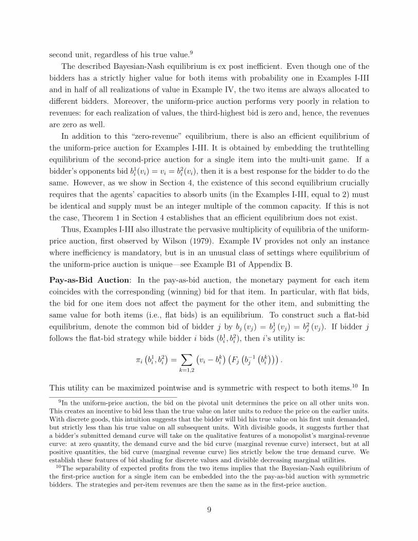
second unit, regardless of his true value.9

The described Bayesian-Nash equilibrium is ex post inefficient. Even though one of the

bidders has a strictly higher value for both items with probability one in Examples I-III

and in half of all realizations of value in Example IV, the two items are always allocated to

different bidders. Moreover, the uniform-price auction performs very poorly in relation to

revenues: for each realization of values, the third-highest bid is zero and, hence, the revenues

are zero as well.

In addition to this “zero-revenue” equilibrium, there is also an efficient equilibrium of

the uniform-price auction for Examples I-III. It is obtained by embedding the truthtelling

equilibrium of the second-price auction for a single item into the multi-unit game. If a

bidder’s opponents bid b1i (vi) = vi = b2i (vi), then it is a best response for the bidder to do the

same. However, as we show in Section 4, the existence of this second equilibrium crucially

requires that the agents’ capacities to absorb units (in the Examples I-III, equal to 2) must

be identical and supply must be an integer multiple of the common capacity. If this is not

the case, Theorem 1 in Section 4 establishes that an efficient equilibrium does not exist.

Thus, Examples I-III also illustrate the pervasive multiplicity of equilibria of the uniform-

price auction, first observed by Wilson (1979). Example IV provides not only an instance

where inefficiency is mandatory, but is in an unusual class of settings where equilibrium of

the uniform-price auction is unique—see Example B1 of Appendix B.

Pay-as-Bid Auction: In the pay-as-bid auction, the monetary payment for each item

coincides with the corresponding (winning) bid for that item. In particular, with flat bids,

the bid for one item does not affect the payment for the other item, and submitting the

same value for both items (i.e., flat bids) is an equilibrium. To construct such a flat-bid

equilibrium, denote the common bid of bidder j by bj (vj) = b1j (vj) = b2j (vj). If bidder j

follows the flat-bid strategy while bidder i bids (b1i , b2i ), then i’s utility is:

πi(b1i , b

2i

)=∑k=1,2

(vi − bki

) (Fj(b−1j

(bki)))

.

This utility can be maximized pointwise and is symmetric with respect to both items.10 In

9In the uniform-price auction, the bid on the pivotal unit determines the price on all other units won.This creates an incentive to bid less than the true value on later units to reduce the price on the earlier units.With discrete goods, this intuition suggests that the bidder will bid his true value on his first unit demanded,but strictly less than his true value on all subsequent units. With divisible goods, it suggests further thata bidder’s submitted demand curve will take on the qualitative features of a monopolist’s marginal-revenuecurve: at zero quantity, the demand curve and the bid curve (marginal revenue curve) intersect, but at allpositive quantities, the bid curve (marginal revenue curve) lies strictly below the true demand curve. Weestablish these features of bid shading for discrete values and divisible decreasing marginal utilities.

10The separability of expected profits from the two items implies that the Bayesian-Nash equilibrium ofthe first-price auction for a single item can be embedded into the the pay-as-bid auction with symmetricbidders. The strategies and per-item revenues are then the same as in the first-price auction.

9

the symmetric case, the distributions of values are identical and the first-order condition

Fj(b−1i

(bki))

=(vi − bki

)fj(b−1i

(bkj)), k = 1, 2, has a symmetric solution bi (·) = bj (·).

The auction then efficiently allocates both items. In the asymmetric case, the equilibrium

strategies are asymmetric and the outcome is inefficient.

Vickrey Auction: In the benchmark multi-unit Vickrey auction, the payment for bidder

i ’s first and second items (if won) is the sum of the first- and the second-highest rejected

bids reported by bidders j 6= i. A bidder has no impact on his own payments and bidding

b1i (vi) = b2i (vi) = vi for i = 1, 2 is weakly dominant for each bidder and constitutes a

Bayesian-Nash equilibrium, which is ex post efficient.

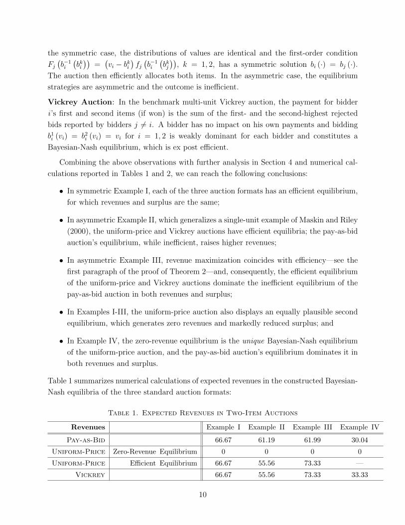
Combining the above observations with further analysis in Section 4 and numerical cal-

culations reported in Tables 1 and 2, we can reach the following conclusions:

• In symmetric Example I, each of the three auction formats has an efficient equilibrium,

for which revenues and surplus are the same;

• In asymmetric Example II, which generalizes a single-unit example of Maskin and Riley

(2000), the uniform-price and Vickrey auctions have efficient equilibria; the pay-as-bid

auction’s equilibrium, while inefficient, raises higher revenues;

• In asymmetric Example III, revenue maximization coincides with efficiency—see the

first paragraph of the proof of Theorem 2—and, consequently, the efficient equilibrium

of the uniform-price and Vickrey auctions dominate the inefficient equilibrium of the

pay-as-bid auction in both revenues and surplus;

• In Examples I-III, the uniform-price auction also displays an equally plausible second

equilibrium, which generates zero revenues and markedly reduced surplus; and

• In Example IV, the zero-revenue equilibrium is the unique Bayesian-Nash equilibrium

of the uniform-price auction, and the pay-as-bid auction’s equilibrium dominates it in

both revenues and surplus.

Table 1 summarizes numerical calculations of expected revenues in the constructed Bayesian-

Nash equilibria of the three standard auction formats:

Table 1. Expected Revenues in Two-Item Auctions

Revenues Example I Example II Example III Example IV

Pay-as-Bid 66.67 61.19 61.99 30.04

Uniform-Price Zero-Revenue Equilibrium 0 0 0 0

Uniform-Price Efficient Equilibrium 66.67 55.56 73.33 —

Vickrey 66.67 55.56 73.33 33.33

10

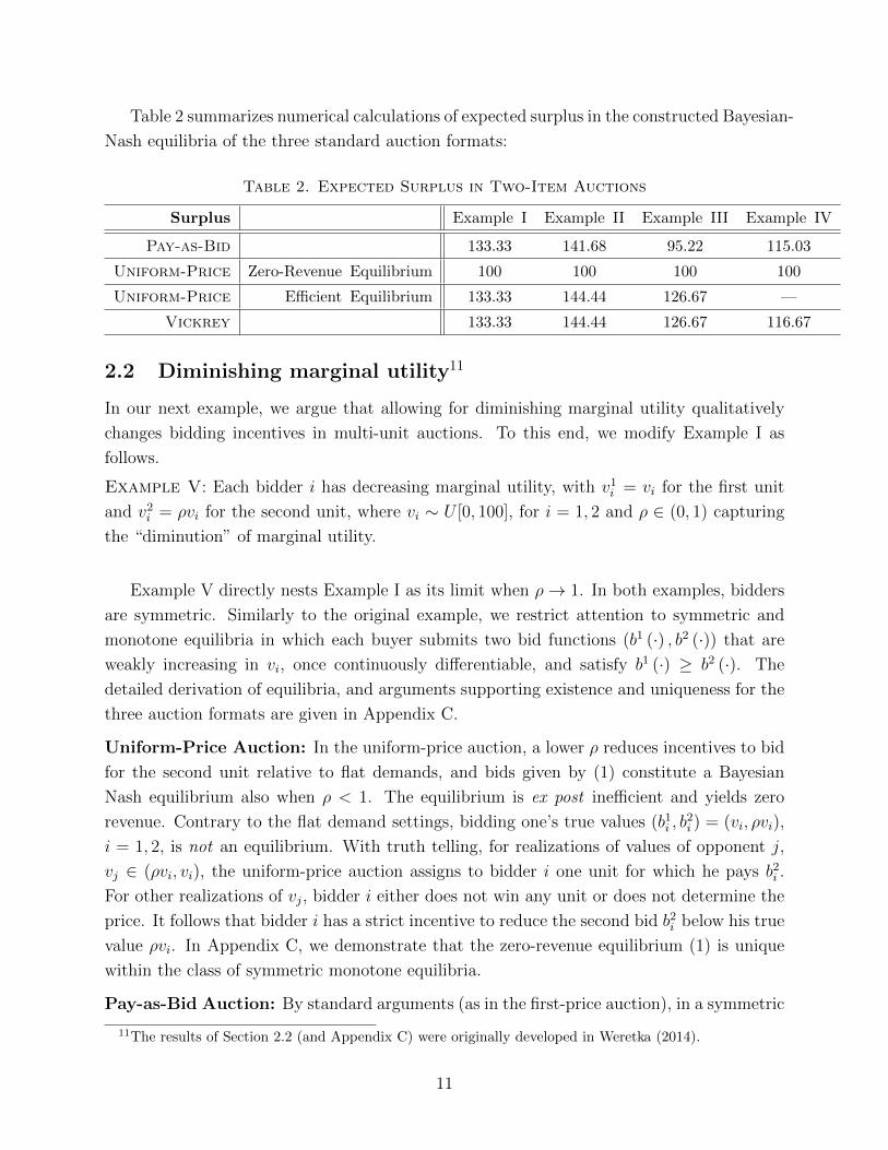
Table 2 summarizes numerical calculations of expected surplus in the constructed Bayesian-

Nash equilibria of the three standard auction formats:

Table 2. Expected Surplus in Two-Item Auctions

Surplus Example I Example II Example III Example IV

Pay-as-Bid 133.33 141.68 95.22 115.03

Uniform-Price Zero-Revenue Equilibrium 100 100 100 100

Uniform-Price Efficient Equilibrium 133.33 144.44 126.67 —

Vickrey 133.33 144.44 126.67 116.67

2.2 Diminishing marginal utility11

In our next example, we argue that allowing for diminishing marginal utility qualitatively

changes bidding incentives in multi-unit auctions. To this end, we modify Example I as

follows.

Example V: Each bidder i has decreasing marginal utility, with v1i = vi for the first unit

and v2i = ρvi for the second unit, where vi ∼ U [0, 100], for i = 1, 2 and ρ ∈ (0, 1) capturing

the “diminution” of marginal utility.

Example V directly nests Example I as its limit when ρ→ 1. In both examples, bidders

are symmetric. Similarly to the original example, we restrict attention to symmetric and

monotone equilibria in which each buyer submits two bid functions (b1 (·) , b2 (·)) that are

weakly increasing in vi, once continuously differentiable, and satisfy b1 (·) ≥ b2 (·). The

detailed derivation of equilibria, and arguments supporting existence and uniqueness for the

three auction formats are given in Appendix C.

Uniform-Price Auction: In the uniform-price auction, a lower ρ reduces incentives to bid

for the second unit relative to flat demands, and bids given by (1) constitute a Bayesian

Nash equilibrium also when ρ < 1. The equilibrium is ex post inefficient and yields zero

revenue. Contrary to the flat demand settings, bidding one’s true values (b1i , b2i ) = (vi, ρvi),

i = 1, 2, is not an equilibrium. With truth telling, for realizations of values of opponent j,

vj ∈ (ρvi, vi), the uniform-price auction assigns to bidder i one unit for which he pays b2i .

For other realizations of vj, bidder i either does not win any unit or does not determine the

price. It follows that bidder i has a strict incentive to reduce the second bid b2i below his true

value ρvi. In Appendix C, we demonstrate that the zero-revenue equilibrium (1) is unique

within the class of symmetric monotone equilibria.

Pay-as-Bid Auction: By standard arguments (as in the first-price auction), in a symmetric

11The results of Section 2.2 (and Appendix C) were originally developed in Weretka (2014).

11

monotone equilibrium, bid functions b1 (·) , b2 (·) are strictly increasing. Bidder i observes

vi and submits (b1i , b2i ) satisfying b1i ≥ b2i . With no benefit from overbidding for the first

unit at vi = 100, b1 (100) = b2 (100) = b, and both bids are from some interval b ∈[0, b].

Let φ1 (·) , φ2 (·) denote corresponding inverses of b1 (·) , b2 (·), satisfying φ2 (·) ≥ φ1 (·). The

marginal bid distribution of buyer j for units k = 1, 2 is Pr[bk (vj) ≤ b

]= F

[φk (b)

]= φk(b)

100.

Bidder i wins two units if the second bid exceeds j′s bid for the first unit, b2i > b1 (vj). The

probability of this event is F [φ1 (b2i )], and he wins one unit if b1i > b2 (vj) and b2i < b1 (vj),

which happens with probability F [φ2 (b1i )] − F [φ1 (b2i )]. Thus, i′s net expected utility is

given by:

πi(b1i , b

2i ) = F

[φ1(b2i)] (

vi + ρvi − b1i − b2i)+ (F

[φ2(b1i)]

− F[φ1(b2i)])(vi − b1i

)=

= F[φ1(b2i)] (

ρvi − b2i)+ F

[φ2(b1i)] (

vi − b1i).

The net utility functions consist of two separate components, each depending on the bid for

one of the two units. The first order conditions and the uniform distribution jointly imply

for any b ∈[0, b]:

[φ1 (b)]′ (ρvi − b) = φ1 (b) ,

[φ2 (b)]′ (vi − b) = φ2 (b) .

By equilibrium symmetry, the optimal bids satisfy b1i = b1 (vi) and b2i = b2 (vi), and hence

[φ1 (b)]′ =φ1 (b)

ρφ2 (b)− b, [φ2 (b)]′ =

φ2 (b)

φ1 (b)− b. (2)

Following the steps analogous to the derivation of equilibrium in the first-price auction with

asymmetric bidders, one can solve the system of differential equations and obtain equilibrium

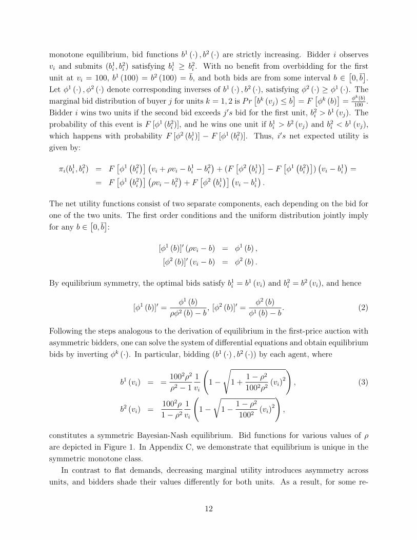
bids by inverting φk (·). In particular, bidding (b1 (·) , b2 (·)) by each agent, where

b1 (vi) = =1002ρ2

ρ2 − 1

1

vi

(1−

√1 +

1− ρ2

1002ρ2(vi)

2

), (3)

b2 (vi) =1002ρ

1− ρ21

vi

(1−

√1− 1− ρ2

1002(vi)

2

),

constitutes a symmetric Bayesian-Nash equilibrium. Bid functions for various values of ρ

are depicted in Figure 1. In Appendix C, we demonstrate that equilibrium is unique in the

symmetric monotone class.

In contrast to flat demands, decreasing marginal utility introduces asymmetry across

units, and bidders shade their values differently for both units. As a result, for some re-

12

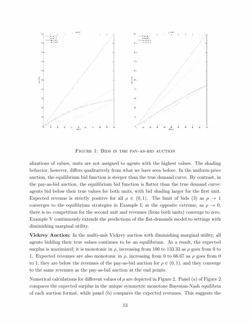
Figure 1: Bids in the pay-as-bid auction

alizations of values, units are not assigned to agents with the highest values. The shading

behavior, however, differs qualitatively from what we have seen before. In the uniform-price

auction, the equilibrium bid function is steeper than the true demand curve. By contrast, in

the pay-as-bid auction, the equilibrium bid function is flatter than the true demand curve:

agents bid below their true values for both units, with bid shading larger for the first unit.

Expected revenue is strictly positive for all ρ ∈ (0, 1). The limit of bids (3) as ρ → 1

converges to the equilibrium strategies in Example I; at the opposite extreme, as ρ → 0,

there is no competition for the second unit and revenues (from both units) converge to zero.

Example V continuously extends the predictions of the flat-demands model to settings with

diminishing marginal utility.

Vickrey Auction: In the multi-unit Vickrey auction with diminishing marginal utility, all

agents bidding their true values continues to be an equilibrium. As a result, the expected

surplus is maximized; it is monotonic in ρ, increasing from 100 to 133.33 as ρ goes from 0 to

1. Expected revenues are also monotonic in ρ, increasing from 0 to 66.67 as ρ goes from 0

to 1; they are below the revenues of the pay-as-bid auction for ρ ∈ (0, 1), and they converge

to the same revenues as the pay-as-bid auction at the end points.

Numerical calculations for different values of ρ are depicted in Figure 2. Panel (a) of Figure 2

compares the expected surplus in the unique symmetric monotone Bayesian-Nash equilibria

of each auction format, while panel (b) compares the expected revenues. This suggests the

13

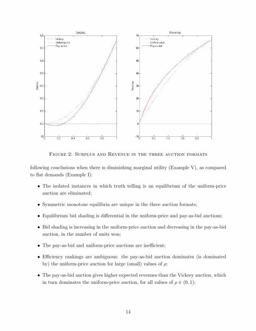
Figure 2: Surplus and Revenue in the three auction formats

following conclusions when there is diminishing marginal utility (Example V), as compared

to flat demands (Example I):

• The isolated instances in which truth telling is an equilibrium of the uniform-price

auction are eliminated;

• Symmetric monotone equilibria are unique in the three auction formats;

• Equilibrium bid shading is differential in the uniform-price and pay-as-bid auctions;

• Bid shading is increasing in the uniform-price auction and decreasing in the pay-as-bid

auction, in the number of units won;

• The pay-as-bid and uniform-price auctions are inefficient;

• Efficiency rankings are ambiguous: the pay-as-bid auction dominates (is dominated

by) the uniform-price auction for large (small) values of ρ;

• The pay-as-bid auction gives higher expected revenues than the Vickrey auction, which

in turn dominates the uniform-price auction, for all values of ρ ∈ (0, 1);

14

• For ρ → 0, all auctions give the maximal surplus of 100 and zero revenue, while for

ρ → 1, the surplus and revenue converge to those in Example I (and, specifically for

the uniform-price auction, the zero-revenue equilibrium).

While the examples of this Section have been special, they are representative of more general

results that will follow. Auctions in settings with flat demands are studied more generally

in Section 4, and auctions in settings with perfectly divisible goods and linearly decreasing

marginal utility are studied in Section 5. Multiplicity of equilibrium is endemic to multi-unit

auctions, making efficiency and revenue comparisons of auction formats potentially problem-

atic. Diminishing marginal utility introduces further strategic aspects. A recurring theme

of our paper is to find compelling ways to make comparisons possible.

3 Model

We make the following general assumptions. Quantity Q of a perfectly-divisible good is

sold to I bidders. Each bidder receives a private signal si ∈ [0, 1] of his value vi before

bids are submitted; this signal will be referred to as the bidder’s type. Let s ≡ {si}Ii=1

and let s−i ≡ {sj}j 6=i. Types are drawn from the joint distribution F with support [0, 1]I

and finite density f that is strictly positive on (0, 1)I . While distribution function F is

commonly known to bidders, the realization si is known only to bidder i. A bidder i with

value vi consuming qi and paying Pi has a payoff ui(vi, qi, Pi), where vi = vi(s). The seller’s

valuation for the good is 0.

An assignment of the good auctioned among bidders Q∗ (s) ≡ (Q∗1 (s) , . . . , Q

∗I (s)) is said

to be ex post efficient if each unit goes to the bidder who values it the most:

Q∗ (s) ≡ arg maxQ1(s),...,QI(s)

{I∑i=1

ui(vi (s) , Qi (s) , 0)

∣∣∣∣∣I∑i=1

Qi (s) ≤ Q

}. (4)

The seller uses a conventional auction to allocate the good. In a conventional auction,

bidders simultaneously and independently submit bids and the items are awarded to the

highest bidders. In the formal analysis we assume that, having observed his signal si, each

bidder i submits a bid function bi(·, si) : [0, Q] → [0,∞) expressing the value bi bid for any

quantity q. We require the function bi to be right-continuous at q = 0, left-continuous at

all q ∈ (0, Q] and weakly decreasing. The market-clearing price p is then set at the highest

rejected bid,

p = min

{p|

I∑i=1

b−1i (p) ≤ Q

},

15

where b−1i is bidder i’s demand function constructed by inverting his bid function.12 If∑

i b−1i (p, si) = Q, then each bidder i is assigned a quantity ofQi ≡ b−1

i (p, si). If∑

i b−1i (p, si) >

Q, then the aggregate demand curve is flat at p, and some bidders’ demands at p will need

to be rationed.13 The pricing rule Pi depends on the auction:

Uniform-Price Auction: Each bidder i assigned Qi pays the market clearing price p for

each of the Qi units obtained; i’s total payment is Pi = Qip.

Pay-as-Bid Auction: Each bidder i assigned Qi pays his winning bids; Pi =´ Qi0bi(y, si)dy.

Note that most other sealed-bid auction formats in the literature (most conspicuously,

the multi-unit Vickrey auction) also satisfy the definition of a conventional auction.

Finally, the equilibrium concept used in this paper is the usual Bayesian-Nash Equilib-

rium, which comprises a profile of bid functions, bi(·, si), for every type of every bidder which

are mutual best responses.

4 Constant Marginal Values

In this section, we study bidders with constant marginal values for the good, up to fixed

capacities, i.e. “flat demands”.

4.1 Assumptions

In the analysis of the flat demands model, we normalize Q = 1 without loss of generality.

Each bidder i can consume any quantity qi ∈ [0, λi], where λi ∈ (0, 1) is a capacity; formally,

we assume that utility from consuming quantities qi > λi is negative. To make the problem

nontrivial, we require that there be competition for each quantity of the good: for each

i,∑

j 6=i λj ≥ 1. One can interpret qi as bidder i’s share of the total quantity and λi as a

12In section with flat demands, an inverse bid b−1i (·, si) is constructed from the bid function as follows.

Given fixed si, let Γ = {(q, bi(q, si))|q ∈ [0, λi]} ∪{(0, P ), (λi, 0)

}, where λi is the capacity of bidder i

(defined in Section 4.1), capacities denote the graph of bi(q) and the two additional points which say that, ata sufficiently high price P , the bidder demands nothing, and at a price of zero, the bidder demands his optimalquantity (denoted λi). Take the closure of Γ, and then fill vertically all the discontinuities of the demandcurve, and call the result Γ′. Define a weakly-decreasing correspondence γi(p) = {q|(q, p) ∈ Γ′}, and definefunction b−1

i (p, si) to be the selection from γi(p) which is left-continuous at p = P and right-continuous at allp ∈ [0, P ). Since each b−1

i (·, si) is weakly decreasing, and since the construction for inverting bid functionsimposes that b−1

i (0) = λi and b−1i (P ) = 0, observe that the market-clearing price p exists and is unique, and

p ∈ (0, P ).13If there is just a single bidder whose demand curve is flat at p, then this bidder’s quantity is reduced

by∑

i b−1i (p, si)−Q. If there are multiple bidders with demand curves flat at p, then quantity is allocated

by proportionate rationing. For our purposes, the specific tie-breaking rule will not matter, since withprobability one, there is at most a single bidder with flat demand at p. Define bidder i’s incrementaldemand at p as ∆i(p) ≡ b−1

i (p, si) − limp↓p b−1i (p, si). Then, bidder i is awarded an amount b−1

i (p, si) −(∑

i b−1i (p, si))−Q)∆i(p)/

∑i ∆i(p).

16

quantity restriction. For example, in the U.S. Treasury auctions, a bidder’s net long position,

including both pre-auction trading and the auction award, cannot exceed 35%. The FCC

spectrum auctions have had similar quantity restrictions.

Bidder i has a constant marginal value vi ∈ [0, 1] for the good up to the capacity λi, and

the bidder’s utility is ui(vi, qi, Pi) = qivi−Pi, for qi ∈ [0, λi]. The relationship between types

si ∈ [0, 1] and values vi (·, ·) is common knowledge among bidders, and is assumed to satisfy

the following:

Assumption 1 (Value Monotonicity) Function vi (si, s−i) is strictly increasing in si,

weakly increasing in each component of s−i, and continuous in all its arguments.

Assumption 2 (Types Rank Values) si > sj ⇒ vi(s) > vj(s).

The model generalizes that of independent private values in two ways: values may de-

pend on the private information of others, and a bidder’s private information need not be

independent of the private information of others. The types rank values assumption deliber-

ately excludes a pure common value model, since in that case any assignment respecting the

capacities λi—and hence any auction that does not have a reserve price and that does not

force bidders to buy more than they want—is efficient.14 Note that the above assumptions

imply that any two ex-post efficient assignments are equal with probability one.

A critical element in the analysis of auctions for a single good is the first-order statistic.

If Yi = max {sj|j 6= i} is the highest signal of bidders other than i, then bidder i receives

the good in the efficient assignment only if si ≥ Yi. In m-unit auctions where each bidder

can win at most one unit, the mth-order statistic serves the analogous role. However, when

analyzing general multi-unit auctions the order statistics by themselves are inadequate: the

quantity won by a bidder confers additional information. We thus appropriately generalize

the first-order statistic notions to a multi-unit auction.

Definition. Fix an efficient assignment Q∗. For any s−i ∈ [0, 1]I−1 and q ∈ (0, λi], define

τ qi (s−i) ≡ inf {si ∈ [0, 1] : Q∗i (si, s−i) ≥ q} , the minimal signal of bidder i such that this

bidder is assigned at least q items in the efficient assignment Q∗. Let F qi (y|x) = Pr{τ qi (s−i) ≤

y|si = x} be the c.d.f. of statistic τ qi (s−i) conditional on i’s own signal, and let f qi (y|x)denote the associated density function. Let wqi (x, y) = E[vi (si, s−i) |si = x, τ qi (s−i) = y]

be an expected value conditional on own signal and statistic τ qi (s−i), and (if defined) let

w+i (x, x) ≡ limq↓0w

qi (x, x).

Note that, with probability one, Q∗(s) is defined uniquely by equation (4). Furthermore,

τ qi (s−i) is defined uniquely for every s−i ∈ (0, 1)I−1 and q ∈ (0, λi]. We will henceforth

assume that the primitives of the model have been specified such that F qi (y|x), f

qi (y|x), and

wqi (x, y), when needed, are mathematically well-defined functions, and such that wqi (x, y) is

continuous in (x, y).

14Section 5 studies a special case of the pure common value model.

17

Essentially all of the previous auction literature has made assumptions that imply the

presence of the Winner’s Curse, the notion that winning is “bad news”: a bidder’s expected

value conditional on winning is less than or equal to his unconditional expected value. In the

single-good case, the standard assumptions postulate that each bidder’s expected value from

the good vi(x, y) ≡ E[vi|si = x, Yi = y] is strictly increasing in x and weakly increasing in

y (Milgrom and Weber, 1982, p. 1100). Our value monotonicity Assumption 1 implies that

wqi (x, y) is strictly increasing in x and weakly increasing in y for all bidders i and quantity

levels q. To extend the Winner’s Curse concept to the multi-unit auction setting, we also

need to capture the idea that winning a larger quantity is “worse news” than winning a

smaller quantity. We thus assume the following.

Assumption 3 (Generalized Winner’s Curse) A multi-unit auction environment ex-

hibits the Generalized Winner’s Curse if, for all bidders i, wqi (x, x) is weakly decreasing in

q. Note that this assumption implies that w+i is well-defined for all bidders i.

4.2 Efficiency

We begin our analysis by noting that, in any of the considered auction formats, an equilibrium

can be efficient only if the bids are flat.

Proposition 1 (Efficient Bids) If a Bayesian-Nash equilibrium of a conventional auc-

tion attains ex post efficiency then all bidders use symmetric, monotonic, flat bid functions:

there exists a strictly increasing function φ : [0, 1] → [0, 1] such that bi(q, si) = φ(si) for

all bidders i = 1, . . . , I, for all quantities q ∈ [0, λi], and for almost every type si ∈ [0, 1].

Moreover, in the uniform-price auction, every bidder i uses the symmetric, flat bid function

bi(q, si) = φ(si) = w+ (si, si), for every type si ∈ [0, 1] and every quantity q ∈ [0, λi].

To see heuristically why efficiency requires flat bidding, consider a symmetric equilibrium

where bi = bj for all bidders i, j. Efficiency requires that the bidder with the highest value,

say bidder i, receives quantity λi. Thus bi (q, si) ≥ bj (0, y) = bi (0, y) for all bidders j 6= i

and signals y < si. The monotonicity and left-continuity of bi allow us to conclude that bi is

flat. We provide a complete proof in the Appendix.

Uniform-Price Auction: Next, we develop the main insight of Section 4: all equilibria of

the uniform-price auction are inefficient. We then finish the equilibrium analysis by looking

at the efficiency of pay-as-bid auctions.

Theorem 1 (Generic Inefficiency of Uniform-Price Auction): Consider a flat-

demand setting that exhibits the Generalized Winner’s Curse. There exists an ex post efficient

equilibrium of the uniform-price auction if, and only if, λi = λ for all i, 1/λ is an integer,

and w+i (x, x) = w+

j (x, x) for all i, j and x.

18

The intuition behind Theorem 1 is that bidders have market power in the uniform-price

auction. If a bidder has a positive probability of influencing price in a situation where the

bidder wins a positive quantity, then the bidder has incentives to shade his bid. In particular,

if a bidder cannot be pivotal for small quantities then he bids his expected values for them. If

the same bidder is pivotal with positive probability for large quantities then he shades his bid

for such quantities. Consequently, his bid cannot be flat, and by the preceding proposition,

the equilibrium is not efficient. We show that such a bidder exists, unless λi = λ for all i

and 1/λ is an integer.

The logic is as follows. By Proposition 1, in an efficient equilibrium each bidder i expects

other bidders j 6= i to submit flat bids. Thus, bidder i’s bids for sufficiently small quantities

are never pivotal: for any subset of other bidders I ′ ⊂ {1, ..., I}−{i} whose combined capacity

satisfies∑

j∈I′ λj < 1, adding a sufficiently small quantity qi to the combined capacity of

bidders in I ′ does not reverse the strict inequality,∑

j∈I′ λj + qi < 1. Thus, bids bi(q, si) for

small quantities q never determine the market-clearing price. Analogous to the reasoning for

the second-price auction of a single item, it will then be optimal for bidder i to maximize

the probability of winning in all events in which the expected value, conditional on winning,

exceeds the payment. Hence bidder i bids bi(q, si) = wqi (si, si) for all small q. This part of

the argument relies on the assumption of a Generalized Winner’s Curse.15

Furthermore, by Proposition 1, in an efficient equilibrium the bid function is constant

for all quantities up to capacity, and hence the necessary condition for efficiency is

bi(q, si) = w+i (si, si) for q ∈ [0, λi]. (5)

This condition is generically violated in a Bayesian-Nash Equilibrium. In the Appendix, we

demonstrate that flat bid bi(q, si) = w+i (si, si) is not a best response for the bidder with the

greatest capacity (say, bidder 1), unless λi = λ for all i = 1, . . . , I and 1/λ is an integer.

Specifically, there exists a subset of bidders other than i = 1, J ⊂ {2, ..., I}, for which∑j∈J λj < 1 and

∑j∈J λj + λ1 > 1. Then, for a quantity threshold L1 ≡ 1 −

∑j∈J λj,

bidding strategy

b1(q, s1) =

{w+

1 (s1, s1) for q ∈ [0, L1]

β for q ∈ (L1, λ1]

},

for β less than but sufficiently close to w+1 (s1, s1), yields a strictly higher payoff than strategy

(5). This is so because with positive probability the signals of all bidders from set J are

higher than s1 while the signals of the remaining bidders are lower than s1, and bidder 1

wins L1 units at price β. Such an event gives bidder i = 1 an incentive to shade his bid for

15In the absence of the Generalized Winner’s Curse, wqi (si, si) > w+

i (si, si) for some q ∈ (0, λi]. Becausebids are constrained to be weakly decreasing in quantity, this violation of the Generalized Winner’s Cursewould imply that bidder i might want to bid more than w+

i (si, si) at some small q ∈ (0, λi] in order to beable to bid higher than w+

i (si, si) at some large q ∈ (0, λi].

19

sufficiently large quantities, q ∈ (L1, λ1].

For an integer 1/λ with λi = λ, the proof of inefficiency does not go through. In this

special case, a bidder affects price only when he wins nothing, and bidding expected value

conditional on winning wqi (si, si) = w+i (si, si) for all qi is a best response. Hence, bids (5) for

all i constitute an equilibrium. Moreover, if w+i (si, si) is identical for all bidders, efficiency

is achieved.

We see that efficiency of the uniform-price auction requires a substantial amount of

symmetry in the model. In environments with interdependent values, the condition that

w+i (x, x) = w+

j (x, x) for any i, j is unlikely to be satisfied without symmetry of value func-

tions, capacities, and distribution of types. By imposing several symmetry assumptions,

we obtain an environment that satisfies the Generalized Winner’s Curse, and we can apply

Theorem 1 to determine when there exists an efficient equilibrium.

Corollary 1 (Symmetric Interdependent Values Model) Consider a flat demands

setting that additionally satisfies:

(i) vπ1 (sπ1 , . . . , sπI ) = v1 (s1, . . . , sI) for any permutation π1, . . . , πI of 1, . . . , I;

(ii) F (sπ1 , . . . , sπI ) = F (s1, . . . , sI) for any permutation π1, . . . , πI of 1, . . . , I;

(iii) (s1, . . . , sI) are affiliated random variables; and

(iv) λi = λ, for all i (i = 1, ..., I).

Then, there exists an ex post efficient equilibrium of the uniform-price auction if, and

only if, 1/λ is an integer.

The above corollary includes, as a special case, the independent private values model

in which individual values (or, equivalently, individual signals) are drawn from the same

distribution. The independent private values environment satisfies the Generalized Winner’s

Curse even if the agents’ values are drawn from different distributions, and thus the following

further corollary obtains.

Corollary 2 (Independent Private Values Model) Consider a flat demands model,

with vi(si, s−i) = si and λi ≡ λ for each i = 1, . . . , I, and with independent but not necessarily

identically distributed Fi (·). There exists an ex post efficient equilibrium of the uniform-price

auction if, and only if, 1/λ is an integer.

Pay-as-Bid Auction: We now establish that in some situations in which efficiency is im-

possible in the uniform-price auction, full efficiency is nevertheless possible in the pay-as-bid

auction. The intuition is straightforward: the inefficiency result in the uniform-price auc-

tion is driven by the incentive for demand reduction due to price impact, in that a bidder

who shades his bids on subsequent units saves money on the purchase of earlier units. By

contrast, this incentive does not exist in the pay-as-bid auction with flat demands; a bidder

20

who reduces his bid for subsequent units (but holds his bids constant on earlier units) does

not realize any savings on his purchase of earlier units.

This is analogous to the situation of a monopolist deciding how much to produce. Recall

that the uniform-price auction is often referred to as a “nondiscriminatory auction” while the

pay-as-bid auction is referred to as a “discriminatory auction.” Just as monopoly without

price discrimination leads to social inefficiency while a monopolist with perfect price discrim-

ination may realize all gains from trade, a nondiscriminatory auction will lead to inefficiency

but a discriminatory auction has the possibility of efficiency. The nondiscriminating monop-

olist’s marginal revenue curve lies strictly below his demand curve, except at zero quantity;

the perfectly discriminating monopolist’s marginal revenue curve may actually coincide with

his demand curve. We therefore obtain supply reduction in the former but not necessarily

in the latter situation.

To construct an efficient Bayesian-Nash equilibrium of the pay-as-bid auction, consider

bidders that have independent private values vi (s) = si and are ex ante symmetric: their

signals si are i.i.d., and their capacities λi = λ are equal for all i. Let Ui(vi) denote the

interim expected utility of bidder i, and let Qi(vi) denote the interim expected quantity

received by bidder i in an efficient direct mechanism. Let m be the greatest integer less than

1/λ, let v−i(m) denote the mth order statistic of signals of all bidders except i, and let F−i(m) (·)

denote its distribution function. Observe that efficiency requires that bidder i must obtain

λ units of the good if vi > v−i(m), 1−mλ units of the good if v−i(m+1) < vi < v−i(m), and 0 units

of the good if vi < v−i(m+1). Thus,

Qi (vi) = λF−i(m) (vi) + (1−mλ)

[F−i(m+1) (vi)− F−i

(m) (vi)]. (6)

Since the interim expected utility of the zero type must equal zero, the usual incentive-

compatibility argument implies that Ui (vi) =´ vi0Qi (x) dx. Now suppose that an efficient

equilibrium of the pay-as-bid auction exists. By Proposition 1, each bidder must use a flat-

bid function almost everywhere: bi(q, vi) = φi(vi). Using this bid function, an alternative

way to calculate the interim expected utility of bidder i is Ui (vi) = Qi (vi) [vi − φi (vi)].

Combining the two expressions for utility gives the equilibrium bid. In the appendix, we

build on this argument to prove the following:

Proposition 2 (Efficient Pay-as-Bid Auction) If bidders have independent private

values vi (s) = si and are ex ante symmetric, i.e., if their signals si are i.i.d., and their

capacities λi = λ are equal, then

bi(q, vi) = φi (vi) = vi −´ vi0Qi (x) dx

Qi (vi)(7)

constitutes an ex-post efficient equilibrium of the pay-as-bid auction.

21

This positive result does not mean that the pay-as-bid auction should be preferred to

uniform pricing. It is well known that a first-price auction for a single indivisible item does

not admit an efficient equilibrium except in special settings. If bidders’ values are random

variables that are not identically distributed, then any equilibrium of the first-price auction

will typically be inefficient. These considerations from the first-price auction carry over to

the current context; the assumption in Proposition 2 that each bidder’s marginal value, vi,

is drawn from the same distribution should be viewed as essential. Proposition 3 treats the

case of asymmetric bidders and easily obtains a negative result.

Proposition 3 (Inefficient Pay-as-Bid Auction) If bidders’ values are independent

but not identically distributed or if their capacities are unequal, then generically there does

not exist an ex post efficient equilibrium of the pay-as-bid auction.

4.3 Ambiguous Rankings of Conventional Auctions

Early discussions of U.S. Treasury auctions conjectured that the uniform-price auction is

superior to the pay-as-bid auction when selling multiple units in terms of both revenue and

efficiency. We have shown above that this conjecture, which derives largely from the analysis

of auctions in which bidders have tastes for only a single unit, is flawed. In uniform-price

auctions, rational bidders strategically submit lower unit prices for larger quantities than for

smaller quantities, even when demands are flat, adversely affecting allocative efficiency. By

contrast, the pay-as-bid auction need not suffer from demand reduction, enabling it to yield

full efficiency in some situations where the uniform-price auction cannot.

We shall now show that in some circumstances the pay-as-bid auction also raises more

revenue than the uniform-price auction. Theorem 2 demonstrates that the efficiency and

revenue rankings of the two auction formats are both ambiguous. We establish this theorem

via two positive results which identify two environments where revenue maximization coin-

cides with full efficiency. Our construction is based on the principle that in any flat-demands

environment, revenues are maximized (subject to no reserve price) by allocating items to

the bidders in descending order of their “marginal revenues,” MRi(vi) = vi − 1−Fi(vi)fi(vi)

, up to

their capacities λi (see Ausubel and Cramton (1999)). We say that the marginal revenues

are monotonic in values if MR(vi) > MR(vj) ⇐⇒ vi > vj.

In the first environment, the pay-as-bid auction attains efficiency while the uniform-price

auction cannot. Consequently, it has the feature that the pay-as-bid auction dominates with

respect to both revenues and efficiency.

Proposition 4 (Dominance of Pay-as-Bid Auction) Consider any symmetric flat-

demands environment in which the marginal revenues are monotonic in values and the bid-

ders’ capacities satisfy λi = λ, for all i = 1, . . . , I. Then, pay-as-bid auction dominates

22

uniform-price in terms of both revenue and efficiency. Furthermore, the dominance is strict

if 1/λ is not an integer.

In the second environment, the uniform-price auction attains efficiency while the pay-

as-bid auction cannot.16 Here, the uniform-price auction dominates with respect to both

revenues and efficiency.

Proposition 5 (Dominance of Uniform-Price Auction) Consider a flat-demand model

in which the bidders’ capacities satisfy λi = 1 for all i = 1, ..., I. Let F be a cdf with support

[v, v], let f be its density, and let its marginal revenue be monotonic in values. Suppose that

vi ∈ [v, v) and each bidder i = 1, ..., I has his value drawn independently from distribution

Fi =F (v)−F (vi)

1−F (vi)on [vi, v]. Then, uniform-price auction dominates pay-as-bid in terms of both

revenue and efficiency. Furthermore, the dominance is strict if there are some i, j such that

Fi 6= Fj.

We prove this proposition in Appendix A. Let us illustrate the forces behind the dom-

inance of the uniform-price auction in the following example. Consider the asymmetric

single-item17 auction environment in which v1 ∼ U [η1, 1], v2 ∼ U [η2, 1], ... , vI ∼ U [ηI , 1],

where 0 ≤ η1 < η2 < . . . < ηI < 1. Observe by an easy calculation that marginal revenues

are monotonic in values, and so revenues are maximized by allocating the item to the bidder

with the highest value. The uniform-price auction now collapses to the second-price auction;

bidding one’s true value, which is the unique equilibrium in undominated strategies, attains

full efficiency and consequently maximizes revenues. We will have established that the equi-

librium of the uniform-price auction dominates the equilibrium of the pay-as-bid auction,

with respect to both efficiency and revenues, provided we can show that the equilibrium of

the first-price auction with these distributions is inefficient. This is demonstrated as follows.

For I = 2 bidders, suppose that the first-price auction has an efficient equilibrium in un-

dominated strategies. For efficiency, bidder 2 must use a monotonic bidding strategy, and

all types v1 < η2 of bidder 1 must win the auction with zero probability. It follows that, for

any ε > 0, type η2 + ε of bidder 2 must bid at least η2 − ε. Otherwise, types v1 ∈ (η2 − ε2, η2)

of bidder 1 could profitably deviate by bidding η2− ε. Define p =12(η1+η2)−η1

1−η1 , the probability

16For simplicity of exposition, we state this and the next proposition assuming no type of bidder i hasvalues between 0 and vi. This violates our modeling assumptions that bidders draw signals from [0, 1]I

and the mapping from signals to values is continuous. One can adapt the propositions to our modelingassumptions by shifting a small mass ε of each bidder’s types to have values in [0, vi). The desired revenueranking will still go through provided that the mass ε is sufficiently small.

17The essential aspects of this counterexample and the preceding proposition do not require a single-unit-demand environment. Alternatively, we could assume that the bidders’ capacities satisfy λi = λ, for all i =1, . . . , I, and 1/λ = M , any integer. However, the efficient equilibrium of the uniform-price auction wouldgenerally no longer be unique; see, for example, the discussion in Section 2.

23

that bidder 1’s type is less than 12(η1 + η2). By bidding 1

2(η1 + η2), every type of bidder 2

can assure himself a payoff of at least 12(η2 − η1)p > 0. Consequently, for ε sufficiently small,

type η2 + ε of bidder 2 does not optimally bid at least η2 − ε, a contradiction. We conclude

that there is no efficient equilibrium of the first-price auction. A similar argument can be

made with more than two bidders.

The above two propositions imply our second major result.

Theorem 2 (Ambiguous Rankings) The efficiency and revenue rankings of the uniform-

price and pay-as-bid auctions are inherently ambiguous.

To summarize, in general, the revenue and efficiency rankings of the two commonly-used

auction formats are ambiguous. However, in all settings with symmetric buyers that we

study, the pay-as-bid auction dominates the uniform-price auction.

5 Diminishing Marginal Values

Apart from affecting bidder’s incentives in the presence of asymmetric information, as ana-

lyzed so far, another aspect of multi-unit demands not present in auctions of unit demands

is the possibility of decreasing marginal utility, which itself introduces new effects, even in

settings where agents’ valuation functions are identical. To study such effects we now allow

bidders to have marginal values that are decreasing in the quantity received. We assume

that the bidders have linear marginal utilities with the same slope and value for the good

(si = v for all i). We examine linear equilibria, in which bids bi(·, v) : R → R+ are linear

in quantity and value.18 The uniqueness of the linear equilibrium allows us to compare the

auction formats in a consistent way.19

18The strategy space is not restricted to the class of linear bids; rather, in a linear equilibrium, it is optimalfor a bidder to submit a linear bid, given that the other bidders play linear strategies. For the uniform-pricemechanism, the linear (Bayesian) Nash equilibrium has been widely used in modeling financial, electricity,and other oligopolistic markets. Hortacsu’s (2002) study of the Turkish Treasury auction and Hortacsu andPuller’s (2008) study of spot market for electricity in Texas find that linear equilibrium provides a gooddescription of the data. Analysis based on non-linear equilibria is developed in Glebkin and Rostek (2014).

19With unbounded support of supply, the linear equilibrium of the uniform-price auction is unique withina large class of equilibria studied by Klemperer and Meyer (1989). They study a model of a procurementauction with an exogenous downward-sloping demand, and show that when utilities are quadratic and uncer-tainty has unbounded support, Nash equilibrium in the uniform-price auction is unique in the set of strategiesthat are piecewise differentiable functions. Their result applies directly to our uniform-price model (witha vertical supply); thus, in our analysis for Generalized Pareto distributions with ξ > 0, the uniform-priceequilibrium is unique within a large class. For distributions with ξ < 0, the set of Nash equilibria in theuniform-price auction is not determinate (but the linear equilibrium is unique). When the utilities are notquadratic, apart from the result by Klemperer and Meyer (1989) that the set of equilibria is connected, noresults are available in the literature about the determinacy of equilibrium in the uniform-price auction. Forthe pay-as-bid auction, Back and Zender (1993), Wang and Zender (2002), and Pycia and Woodward (2014)prove the uniqueness of equilibrium.

24

We identify the class of distributions that admits a linear equilibrium and provide revenue

rankings for all distributions in this class. Decreasing marginal utility changes bidding

incentives and equilibrium properties: Bidders shade their bids even if they have no private

information; in particular, a traditional Bertrand-style argument does not apply and no

auction format allows the seller to extract full surplus, even in the limit as the number

of bidders grows to infinity. Moreover, even though equilibria are ex post efficient (i.e.,

Q (s) = Q∗ (s)), seller revenue varies across auction formats. In particular, with any finite

number of bidders, the pay-as-bid auction brings strictly higher expected revenue than the

uniform-price auction.

5.1 Assumptions

Each bidder i’s marginal utility is affine with common slope ρ > 0 and intercept v ∈ R, thatis ∂u(qi)/∂qi = v−ρqi where u(qi) is the quadratic utility of bidder i. The value v is random

and commonly known to all bidders (i.e., si = v for all i), but not the seller. Bidders are

uncertain about the supply Q being auctioned. The joint c.d.f., F (v,Q) of the value v and

supply Q—which can be correlated—is common knowledge and has non-degenerate support

F (·|v). We make the usual assumption for the quadratic model that for all values of v and

Q in the support of F , the bidders prefer more of the good rather than less; that is, bidders

are not satiated. This last assumption implies that the support of Q is compact for any v.20

5.2 Linear Equilibrium

If the marginal utility was constant, bidding bi(qi, v) = v would be a linear Nash equilibrium

in both uniform-price and pay-as-bid auctions. In such an equilibrium, bidders would not

shade their bids, and both auctions would be revenue maximizing; hence, they would also be

revenue equivalent. None of these predictions obtains when marginal utility is decreasing,

ρ > 0.

Our derivation exploits the following feature of linear equilibrium with downward-sloping

demands: Given a profile of bid functions bj (·, v), j 6= i, bidder i trades against an upward-

sloping, linear (residual) supply p = x+µiqi where the intercept x = x(Q) is a deterministic

function of value v and quantity Q. Market clearing implies that qi +∑

j 6=i b−1j (p, v) =

Q, and with symmetric bids bj = bj′ the slope of the residual supply is given by µi =

− (1/ (I − 1)) ∂bj (·, v) /∂qj (Propositions 6 and 7 below establish that the linear equilib-

rium is symmetric in both the uniform-price and pay-as-bid auctions). For bidder i, the

distribution of the intercept x derived from F (·|v) and µi contains all of the payoff-relevant

information about the strategies of other bidders.

20The non-satiation assumption is not needed for any of the equilibrium characterization in Section 5.2.We use it only in Proposition 6 in Section 5.3.

25

Uniform-Price Auction: The first-order condition equates marginal utility with marginal

payment at each realization of supply; that is, order shading is

v − ρqi − bi = µiqi. (8)

Aggregating the bids of bidders other than i gives i’s residual supply, the slope of which—i’s

price impact—can be characterized as

µi =

(∑j 6=i

(µj + ρ)−1

)−1

. (9)

The unique, symmetric solution to I equations (9) gives the equilibrium price impact of

bidder i equal to µi = ρ/ (I − 2), for I > 2.21 Proposition 6 characterizes equilibrium bids.

Proposition 6 (Equilibrium in Uniform-Price Auction) Suppose I > 2. In the

unique linear equilibrium, the strategy of each bidder is

bi(qi, v) = v −(I − 1

I − 2

)ρqi. (10)

Note that, with decreasing marginal utility, the equilibrium bids remain optimal ex post,

when supply is known.22 By best-responding with a downward-sloping bid, a bidder effec-

tively conditions on the realization of supply, Q, thereby hedging away supply uncertainty.

Furthermore, for any qi the bid bi(qi, v) affects a bidder’s payoff only for the realization of

Q = Iqi.

In contrast to the flat demands model—in which the winning bids do not affect the

equilibrium price unless capacities are heterogeneous, or 1/λ is not an integer, or supply

is sufficiently large—with decreasing marginal utility, the winning bids affect the revenue

irrespective of the level of supply. In linear equilibrium, bid shading v − ρqi − bi = qiµi

is increasing in quantity, and the corresponding bid function (10) is steeper than marginal

21Wilson’s (1979) characterization of equilibrium in the uniform-price auction includes the case of I = 2while assuming constant marginal utility. Non-existence of equilibrium with two bidders for decreasingmarginal utility is standard (e.g., Kyle (1989)).

22Proposition 6 and its argument extend to a more general model with private information and interde-pendent values, a setting we analyzed in 2007 draft of the second of the papers subsumed by the presentmerged work. For independent private values, no restrictions on (nondegenerate) distributions of values arerequired. For interdependent values, Rostek and Weretka (2012) characterize the necessary and sufficientcondition for the ex post property of equilibrium (see also Vives (2011). With private information, theequilibrium assignment is generically inefficient due to the increasing-in-quantity bid shading: a high-valuebidder is shading more than a low-value bidder at the market-clearing price. Since quantity is assigned basedon the bids, the high-value bidder wins too little and the low-value bidder wins too much, relative to theefficient allocation. That is, uniform pricing gives large bidders incentives to make room for smaller bidders.In multi-unit auctions—with flat or decreasing marginal utility—it’s not shading per se but differential bidshading that gives rise to inefficiency.

26

utility. Note also that the payment structure of the uniform-price mechanism together with

the decreasing marginal utility imply that even if the bidders were not to shade their bids,

they would retain a strictly positive surplus.

Pay-as-Bid Auction: Unlike the uniform-price auction (and the Vickrey auction), while a

downward-slopping bid function allows conditioning on the realization of Q in the pay-as-bid

auction, linear equilibrium in the pay-as-bid auction is not an ex-post equilibrium. The value

of bid bi(qi, v) affects the payment for all realizations of supply larger than Q. Thus, the

distribution of supply matters for trade-offs and hence for optimal bids.

Let G(·) denote the c.d.f. and g(·) the density function of the distribution of per capita

supply Q/I, derived from the supply distribution F (·|v) (in the notation we suppress the

dependence of G and g on v). The inverse hazard rate of the equilibrium quantity is defined

as h(·) ≡ (1−G(·))/g(·). When written to reveal the structure of bid shading and the role

of market power, the first-order condition is

v − ρqi − bi = h(qi)[µi − ∂bi(·)/∂qi]. (11)

For any qi, the marginal benefit—measured as the marginal utility net of the bid obtained in

state Q = qiI—is equal to the cost of increased payments in all states with higher realization

of supply. In the Euler equation (11), the cost is thus weighted by the inverse hazard rate

h(·), which captures probabilistic importance of higher realizations of supply.

The dependence of the optimal bid on the distribution of equilibrium quantity raises

the question of which distributions F (·|v) admit linear best responses. Since in a linear

equilibrium µi and ∂bi(·)/∂q are constants, the Euler equation (11) defines a linear schedule

only if h(·) is linear. Lemma 1 characterizes the class of all distributions F (·|v) that exhibita linear inverse hazard rate h (·).

Lemma 1 (Linearity of h(·)) The inverse hazard rate h(·) of per capita supply Q/I is

linear if, and only if, F (·|v) belongs to the class of Generalized Pareto distributions.

The c.d.f. of a Generalized Pareto distribution is given by F (Q|v) = 1 − (1 + ξQ−ασI

)−1ξ ,

where ξ ∈ R is the shape parameter, α ∈ R is the location parameter, and σI > 0 is the scale

parameter. The per-capita supply Q/I is then distributed according to Generalized Pareto

with the inverse hazard rate h(q) = σ− ξα+ ξQI. The Generalized Pareto class encompasses

distributions with decreasing (ξ < 0), constant (ξ =0), and increasing (ξ > 0) inverse hazard

ratios; and has a lower bound of support given by α.23

23Whenever ξ < 0, the support also has an upper bound, equal to −(I − ξ)/ξ. Among distributions withcompact support, ξ = −1 corresponds to a uniform distribution; for ξ = 0 (exponential distribution) andξ > 0 (the class of Pareto distributions), the support is unbounded. Conveniently, the linearity of an inversehazard ratio is preserved under additive (i.e., changing the location) or positive multiplicative (i.e., changingthe scale) transformations of a random variable.

27

Order shading in the pay-as-bid auction can now be understood through the properties of

the supply distributions. Namely, order shading inherits monotonicity in quantity through

the inverse hazard ratio and is decreasing, constant, and increasing in quantity for ξ < 0,

ξ = 0, and ξ > 0, respectively. By contrast to the uniform-price auction, the bid in the

pay-as-bid auction is shaded at zero quantity, and for all distributions with compact support

(ξ < 0), the bid coincides with the marginal utility at the upper end of the support, where

the externality on the payments in higher states vanishes. In the uniform-price auction,

there is no shading at zero quantity, and bids are strictly below the marginal utility at

the upper-end quantity. Moreover, order shading in the pay-as-bid auction need not be

increasing in quantity. Except when ξ = 0 (exponential distribution), the Generalized Pareto

class induces bids that can be flatter (ξ < 0) or steeper (ξ > 0) than the marginal utility,

which reflects the decreasing and increasing with quantity, respectively, relative importance

of higher states.

Observe that when the support of the equilibrium quantity is bounded away from 0,

the optimal bid is flat for small quantities and decreasing for large quantities, which is

inconsistent with linear bidding. To rule out flat-bid parts, we set the lower bound of the

support of Q to zero.

Assumption 4 (Generalized Pareto Distribution: Location Parameter) For

any v, F (·|v) is a Generalized Pareto distribution with location parameter α = 0.

Without imposing bid symmetry, price impact in the pay-as-bid auction is

µi =

(∑j 6=i

(ξµj1− ξ

+ρ

1− ξ

)−1)−1

. (12)

Unlike in the uniform-price auction (Equation (9)), the price impact of bidder i can depend

negatively on the price impact of other bidders; this occurs when ξ < 0. With higher market

power, other bidders are induced to shade more, which makes their inverse bids more elastic,

thereby reducing the price impact of bidder i. To close the model, we determine equilibrium

µi from the first-order condition and bid symmetry, µi = ρ/ (I(1− ξ)− 1). Proposition 7

characterizes equilibrium bids.24

Proposition 7 (Equilibrium in Pay-as-Bid Auction) Suppose ξ < (I − 1)/I. In the

24This strategic interdependence explains why, in the pay-as-bid auction, a linear equilibrium exists evenwith two bidders. However, when ξ exceeds (I − 1)/I, linear equilibrium fails to exist because of theamplification of price impacts, similar to their amplification in the uniform-price auction. The non-satiationassumption implies that ξ < 0, but our equilibrium characterization remains valid for nonnegative ξ. Thecharacterization of the set of (possibly non-linear) Nash equilibria by Wang and Zender (2002) is providedfor a class of supply distributions that is a strict subset of ours. We focus on linear equilibria and Proposition7 characterizes equilibrium bids in all environments that admit linear equilibria.

28

unique linear equilibrium, the strategy of bidder i is

bi(qi, v) = v − (I − 1)ρ

I(1− ξ)− 1

(qi +

I

I − 1σ

). (13)

By Proposition 7, bid shading in the pay-as-bid auction depends on the distribution of

supply. Bid shading is proportional to the inverse hazard rate, and unlike in the case of

flat demands (Proposition 2) shading can decrease or increase in quantity, as determined

by the sign of parameter ξ. With compact support, ξ < 0 and the bidding involves no

shading at the upper end of the support of the per-capita supply. At this quantity, there is

no negative effect on the payments for higher realizations of supply, and the bid coincides

with the marginal value.

With decreasing marginal utility, bidders shade their value regardless of auction size,

including in the limit as I → ∞; this contrasts with the uniform-price auction. Although

in all auction formats considered bidders have no impact on equilibrium price in the com-

petitive auction limit (Equations (9) and (12)), uncertainty still affects order shading in the

pay-as-bid auction (Equation (11)), as the bids still determine the payments for the items

won. Observe further that, in markets with ξ < 0, equilibrium converges more slowly to the

price-taking limit in the pay-as-bid than in the uniform-price auction. The reduction of price

impact via aggregation brought about by additional participants in the pay-as-bid auction

is partially offset by the steepening of individual bids.

5.3 Revenue Rankings

This section presents comparative analysis of revenue in the uniform-price, pay-as-bid, and

the Vickrey auctions against the benchmark of total social surplus.25 In the Vickrey auction,

for the qth unit, bidder i is charged the reported marginal value of the item by other bidders

if q units are reallocated efficiently to other bidders. Thus, the total Vickrey payment of

bidder i is given by the opportunity cost to others and corresponds to the area below his

residual supply. We examine strategic and competitive auctions, and consider risk-averse as

well as risk-neutral preferences of the bidders and of the seller. Assumption 4 is maintained.

Theorem 3 establishes expected revenue rankings: Even though the optimal bidding in

the pay-as-bid auction depends on the supply distribution, the comparison of the mecha-

nisms does not. Let RU , RD, and RV denote the equilibrium revenues in the uniform-price,

25In our setting, the (sealed-bid) Vickrey auction is equivalent to the ascending-bid clinching auctionproposed by Ausubel (2004). Note also that the total surplus can be fully extracted. Recall that si = vfor all i, and consider the following mechanism. Bidders report types v1, v2, ..., vI . Bidders with the highestreports, vi = max (v1, v2, ..., vI), receive Q/I units, where I ≥ 1 is the number of the bidders with the

maximal bid, and they pay their reported surplus viQI − 12ρ(Q/I

)2. Bidders with lower reports receive and

pay zero. By a Bertrand-type argument, the bidders bid truthfully in the unique Nash equilibrium, and theseller extracts the entire surplus.

29

pay-as-bid (discriminatory), and Vickrey auction, respectively, and let TS be the total social

surplus, all in per-capita terms.

Theorem 3 (Expected Revenue Ranking) In the unique linear equilibrium, for any v,

E(TS|v) > E(RD|v) > E(RV |v) > E(RU |v), (14)

whenever equilibria exist.

Consistent with a conjecture often invoked in the literature, the uniform-price design

fosters more aggressive bidding in all the environments considered (see the proof of the

theorem). Nevertheless, the benefit from smaller expected bid shading is not sufficient for the

uniform-price to outperform the pay-as-bid auction in terms of seller’s revenue. Dominance of

the pay-as-bid auction with symmetric bidders is consistent with Proposition 4 and Example

V.26

The revenue dominance of the Vickrey auction over the uniform-price auction can be

strengthened: the Vickrey auction is preferred by the seller regardless of the realization of v

and Q, and, hence, regardless of the seller’s risk attitude.

Proposition 8 (Ex Post Revenue Ranking) For any realization of v and Q, the seller’s

revenue satisfies TS ≥ RV ≥ RU , and both inequalities are strict whenever Q > 0. In

particular, for any strictly increasing utility function of the seller u(·), in the unique linear

equilibrium,

E(u (TS) |v) > E(u(RV)|v)> E(u

(RU)|v). (15)

Since the equilibria of the Vickrey auction and the uniform-price auction are both ex post

equilibria, the ex post dominance of the Vickrey auction over the uniform-price auction does

not depend on the distributional assumptions. Furthermore, the dominance is consistent with

Example V. In contrast to the Vickrey and uniform-price formats, the seller’s preference for

the pay-as-bid does depend on his risk attitude as we show in Proposition 9 below.

As the number of bidders increases, the expected revenue increases both absolutely and as

as a fraction of the expected total surplus E(TS|v). The ranking from Theorem 3 must hold

at least weakly in the limit as I → ∞ (a competitive limit). In fact, if we increase the number

of bidders while keeping the distribution of per capita supply fixed, then the three auctions

yield the same expected revenue in the competitive limit. Nevertheless, the common limit

26In a study of Turkish Treasury auctions, Hortacsu and McAdams (2010) found that the pay-as-bidauction leads to higher revenues than the revenue obtainable from the Vickrey auction, which the authorsattributed to the allocational inefficiency in a pay-as-bid auction with heterogenous bidders. Our resultshows that the pay-as-bid auction brings higher revenue than the Vickrey auction even when the allocationis efficient in both.

30

revenue does not extract the total surplus of E(TS|v); fraction σρ/ (v (1− 2ξ)− σρ) > 0 of

the total surplus is not extracted,

E(TS|v) > limI→∞

E(RV |v) = limI→∞

E(RU |v) = limI→∞

E(RD|v).

In the competitive limit, the residual supply of each bidder is perfectly elastic, and in the

uniform-price auction, bidding becomes truthful, as in the Vickrey auction. With pay-as-bid

pricing, by contrast, bidders still shade their marginal utility (see Equation (13)). Thus,

the reasons underlying the seller’s inability to extract surplus differ across the mechanisms:

in the pay-as-bid auction, it is due to bid shading, whereas in the other two designs, it is

attributed to the payment structure itself, which leaves part of surplus to the bidder.27

Less-than-full surplus extraction, even with symmetric information, is another instance

of new effects brought by diminishing marginal utility that will hold outside of the setting

analyzed here, in any equilibrium with downward-sloping bids. The less-than-full surplus

extraction is also different from large auctions in single-unit demand settings where full

surplus extraction, and hence revenue equivalence, has been established by the literature

on information aggregation, cf. Pesendorfer and Swinkels (1997) and Kremer (2002). One

insight from our simple setting with symmetric information is that the competitive-market

result does not follow from the standard revenue equivalence theorem for unit demands. In

all three auction formats, the allocation is efficient, while the revenue is strictly lower than

the total surplus, which can be extracted (Footnote (25)).

With a finite number of bidders, a risk-averse seller faces a risk-revenue tradeoff when select-

ing an auction format. First, consider the competitive limit in which no such trade-off arises.

By the equality of expected revenue in the competitive limit, a risk-neutral seller concerned

about the expected revenue will be indifferent among the three mechanisms. Proposition

9 asserts that a risk-averse seller strictly prefers the uniform-price auction to the pay-as-

bid auction when there are sufficiently many bidders and the bidders’ marginal utility is

decreasing.

Proposition 9 (SOSD) For any strictly concave increasing utility function u(·), in the

unique linear equilibrium, there exists I such that for any I ≥ I,

E(u(TS)|v) > E(u(RV )|v) > E(u(RU)|v) > E(u(RD)|v).27In a study of large auctions, Swinkels (2001) obtained expected-revenue equivalence between the uniform-

price and pay-as-bid auctions in an indivisible good, multi-unit demand setting with independent privatevalues. Our model is a continuous-bid, complete information counterpart of his setting.

31

In the limit,

limI→∞

E(u(TS)|v) > limI→∞

E(u(RV )|v) = limI→∞

E(u(RU)|v) > limI→∞

E(u(RD)|v).

Theorem 3 and Proposition 9 jointly define a trade-off faced by a seller when choosing

an auction design in markets with strategic bidders. With sufficiently large I, the pay-as-bid

auction gives higher expected revenue but also higher risk than the uniform-price auction.

More generally, for any number of bidders, risk averse preferences exist for which either

format is strictly preferred by the seller: For any I sufficiently high, the c.d.f. of the revenue

induced by the uniform-price auction crosses (once) the c.d.f. of the revenue in the pay-as-bid

auction from below (as shown in the proof of Proposition 9). At the same time, Theorem 3

implies that the second-order stochastic dominance does not extend to auctions with a small

number of bidders. Our results suggest that the uniform-price auction is more likely to be

superior in markets with many bidders, whereas the pay-as-bid might be favored in small

markets.

5.4 Entry

An important lesson from auction theory with single-unit demand is that a seller should favor

auction formats that encourage greater participation (e.g., Bulow and Klemperer (1996)).

With an additional bidder, other participants bid more aggressively. This recommendation is

even more relevant in the context of divisible good auctions with decreasing marginal utility:

apart from the competitive effect, additional participants increase the total surplus in the

auction, even if bidders have identical marginal utilities. For quick intuition, consider a

seller offering two units of a good to identical bidders with utility function u (q) = 2q−0.5q2.

Allocating the two units to one bidder brings the total surplus of 2, but allocating the good

to two bidders so that each bidder receives one unit, increases the total surplus to 3. If

the identical demands were flat, the total surplus would be independent of the number of

bidders.

Let us allow an infinite pool of potential entrants in the model. Having learned v, the

bidders—simultaneously or sequentially—choose whether or not to join an auction. Entry

incurs a fixed cost c. Given the exogenous distribution of Q, per capita supply depends on

the number of entrants. Consider pure strategy Subgame Perfect Nash equilibria such that

the entrants submit linear bids in the bidding stage. Barring indifference, the number of

entrants equals the maximal integer for which the expected bidder’s payoff is greater than c.

Our main observation regarding entry is that, in any equilibrium, the uniform-price

auction encourages weakly more entry than the Vickrey auction, which in turn encourages

weakly more entry than the pay-as-bid auction; there exist values of parameters for which

the inequalities are strict. In equilibrium, the uniform-price auction leaves more surplus

32

to the bidders; given the fixed number and symmetry of the bidders, the allocations in all

auction formats are Pareto efficient, and the total surplus is shared between the bidders and

the seller. The ranking of entry then follows from the revenue rankings of Theorem 3. The

weak relative advantage of the uniform-price design in encouraging entry is consistent with

the evidence from the U.S. Treasury experiment.

The entry advantage of the uniform-price auction turns out to be sufficient to reverse

the revenue rankings established for auctions with a fixed number of participants. A small

difference in the number of bidders translates into a significant revenue change, due to the

surplus effect as well as the competitive effect. As a result, there are parameter values

such that the uniform-price auction dominates the other auction formats in both expected

revenue and participation. Thus, Friedman’s conjecture about participation margin giving

an advantage to the uniform-price auction holds even without information acquisition.

Ignoring the integer problem, one can show that the endogenized number of participants

exceeds the Pareto efficient auction size in all three auction formats—an argument in favor

of the pay-as-bid auction. In all auction formats, excess entry arises because each bidder

ignores the negative externality of his participation on the net utility of other bidders. For

auctions of single items, Levin and Smith (1994) demonstrate that auctions encourage entry

levels that are excessive from a social point of view.

6 Conclusions

Multi-unit auctions differ from single-unit auctions in essential ways. Most fundamentally,

the classic efficiency result for the second-price auction of a single item does not extend

to the uniform-price auction of many items. In the uniform-price auction, winning bidders

affect the market price with positive probability. Hence, bidders have incentives to reduce

their demands, upsetting both the strategic simplicity and the efficiency of uniform-price

auctions. By shading his bid for marginal items, the bidder is able to reduce the expected

price paid on inframarginal items. The more one buys, the greater the incentive to shade.

As a result, large bidders will sometimes lose against small bidders on items that the large

bidders value more highly.

In this paper, we prove the general inefficiency of the uniform-price auction. Differential

incentives to shade bids arise whenever a winner influences the market-clearing price with

positive probability. The only cases that escape our inefficiency result are: (1) pure common

values, in which all assignments are efficient, and (2) single-unit demands and analogous

cases, where a bidder determines the price only when the bidder wins zero quantity.

An implication of the inefficiency result is that there is a class of environments (namely,

symmetric private value auctions) in which the symmetric equilibrium of the oft-criticized

pay-as-bid auction dominates all equilibria of the uniform-price auction in both efficiency and

33

seller revenues. However, relaxing the symmetry and risk-neutrality assumptions leads to a

class of environments where the uniform-price auction outperforms the pay-as-bid auction

in both efficiency and revenues. Determining the better pricing rule is therefore an empirical

question.

The practical importance of demand reduction is easily seen in spectrum auctions. Our

theorems do not directly apply to the spectrum auctions, since the FCC and others used a

simultaneous ascending auction and, often, the licenses are not perfect substitutes. Hence,

the analogy between our setting and the spectrum auctions is crude. Still, based on the expe-

rience of many spectrum auctions around the world, we conclude that demand reduction is of

fundamental importance to bidders. Indeed, demand reduction is likely more pronounced in

simultaneous ascending auctions than in sealed-bid auctions, since the bidders can propose

divisions of the licenses through their early bids.28 The October 1999 German auction of

GSM spectrum, in which ten spectrum blocks were offered and the two principal bidders won

five apiece, illustrates this behavior most clearly. The auction lasted just two rounds—one

to propose the split and one to accept it.

Direct evidence of strategic demand reduction was observed in the FCC’s Nationwide

Narrowband Auction. In round 11, PageNet decided to cut back from bidding on three large

licenses to two (Cramton 1995). PageNet felt that, if it continued to demand a third large

license, it would drive up the prices on all of the large licenses to disadvantageously-high

levels. Hence, it made sense to reduce its demand to two, even though the auction price

had not yet reached PageNet’s incremental value for a third large license. In making this

decision, it was essential for PageNet to anticipate the effect of demand reduction on prices.

Anticipating price movements as a function of one’s demand is often guesswork. Still

the consequences of guessing wrong can be dramatic, as was illustrated in the August 2000

German auction of third-generation (3G) mobile wireless licenses. After round 127, Deutsche

Telekom could have likely brought the auction to a rapid close by reducing its demand from

three license blocks to two. Instead, Deutsche Telekom continued bidding for three blocks

for some 40 more rounds, ultimately buying the two license blocks that it could have bought

earlier, but paying about $2 billion extra.

As in experiments, real-world bidders learn from their mistakes. Three months later,

in November 2000, the Austrian 3G auction was held, with essentially the same rules and

essentially the same players as the German auction. The starting prices in the Austrian

auction were one-seventh of the final German prices (on a population-adjusted basis) and

there were sufficiently few bidders that all could be winners if they reduced their demands.

All but one of the bidders engaged in demand reduction at the first opportunity and there was

a wide presumption that the one holdout, government-owned Telekom Austria, was under

severe political pressure to prevent the auction from ending. Even then, demand reduction

28See, for example, Ausubel and Schwartz (1999).

34

did well at predicting the outcome: the auction ended in just 14 rounds, at prices only 15%

above the low starting prices, and with most participants shading their marginal bids well

below their presumed values.

Another important application is in wholesale electricity markets. With only a few excep-

tions, these are uniform-price auctions conducted daily by the system operator. Our theory

applies directly, accounting for the strategic supply reduction in response to uniform pricing

in a procurement auction. The incentive to inflate bids grows with the quantity supplied,

since the higher price is enjoyed on the larger quantity. Wolfram (1998) found compelling

evidence of supply reduction in the early years of the UK electricity market. In 2001, the UK

switched from uniform pricing to pay-as-bid pricing. The study by Borenstein, Bushnell, and

Wolak (2002) of why electricity expenditures in California’s restructured wholesale market

rose from $2 billion in summer 1999 to $9 billion in summer 2000 found that over one-half

of this increase was attributable to market power. In response to the crisis, the California

Power Exchange considered switching from uniform to pay-as-bid pricing. Unlike in the UK,

the proposal was rejected (Kahn et al. 2001).

We present this experience from electricity and spectrum markets to highlight the prac-

tical importance of demand reduction, rather than necessarily as an argument against the

uniform-price auction. Uniform pricing has several desirable properties, including: (1) it is

easily understood in both static and dynamic forms, (2) it is fair in the sense that the same

price is paid by everyone, (3) absent market power it is efficient and strategically simple

(“you just bid what you think it’s worth”), and (4) the exercise of market power under

uniform pricing favors smaller bidders. While the first three points are commonly made in

practice, it is the fourth point that may decisively favor uniform pricing in many practical

settings, including some spectrum and electricity markets.

Competition and innovation are often fostered by market designs that encourage the

entry and success of small participants. Pay-as-bid pricing disadvantages small bidders:

profits depend critically on the bidder’s ability to guess the clearing price, and this ability

grows with size. In sharp contrast, uniform pricing levels the playing field by weakening the

penalty for guessing wrong. At the same time, the current paper has shown that uniform

pricing also creates an incentive for large bidders to make room for their smaller rivals.

In his original proposal, Milton Friedman (1960, p. 65) recognized the informational

leveling effect of uniform pricing: “This alternative, in any of its variants, will make the

price the same for all purchasers, reduce the incentive for collusion, and greatly widen the

market.” We add to Friedman’s effect the demand reduction effect, which cuts in the same

direction. The Treasury auction experiment provides empirical support for the prediction

that uniform pricing widens market participation: the five-firm concentration ratio declined

by 10 percentage points in auctions that were changed from pay-as-bid to uniform pricing

(Malvey and Archibald 1998). The uniform-price auction is not a panacea, since unlike its

35

unit-demand counterpart it inevitably yields inefficiency, whereas some alternative multi-unit

designs do not (see Vickrey (1961) and Ausubel (2004)). Nonetheless, good market design

should encourage the evolution toward more competitive market structures, and uniform

pricing does just that.

References

Armantier, O. and E. Sbai (2006): “Estimation and Comparison of Treasury Auction Format

when Bidders are Asymmetric,” Journal of Applied Econometrics, 21, 6, 745-79.

Ausubel, L. M. (2004): “An Efficient Ascending-Bid Auction for Multiple Objects,” American

Economic Review , 94, 5, 1452-75.

Ausubel, L. M. and P. Cramton (1999): “The Optimality of Being Efficient,” Working Paper.

Ausubel, L. M. and J. A. Schwartz (1999): “The Ascending Auction Paradox,” Working

Paper.

Back, K. and J. F. Zender (1993): “Auctions of Divisible Goods: On the Rationale for the

Treasury Experiment,” Review of Financial Studies, 6, 733-64.

Bolle, F. (1997): “Necessary Conditions for Efficient Multiple-Bid Auctions,” in R. Nau, E.

Gronn, M. Machina and O. Bergland, eds., Economic and Environmental Risk and Uncertainty:

New Models and Methods, Boston: Kluwer Academic Publishers, 123-143.

Borenstein, S., J. B. Bushnell, and F. A. Wolak (2002): “Measuring Market Inefficiencies

in California’s Restructured Wholesale Electricity Market,” American Economic Review , 92, 5,

1376-1405.

Brenner, M., D. Galai and O. Sade (2009): “Sovereign Debt Auctions: Uniform or Discrimi-

natory?,” Journal of Monetary Economics, 56, 267-274.

Bulow, J. I. and P. D. Klemperer (1996): “Auctions vs. Negotiations,” American Economic

Review , 86, 180-194.

Chapman, J. T. E., D. McAdams, and H. J. Paarsch (2007): “Bounding revenue compar-

isons across multi-unit auction formats under best response,” American Economic Review , 97, 2,

455–458.

Cramton, P. (1995): “Money Out of Thin Air: The Nationwide Narrowband PCS Auction,”

Journal of Economics and Management Strategy , 4, 267-343.

Engelbrecht-Wiggans, R. (1988): “Revenue Equivalence in Multi-object Auctions,” Economics

Letters, 26, 15-19.

Engelbrecht-Wiggans, R., J. A. List, and D. Lucking-Reiley (2006): “Demand Reduc-

tion in Multi-unit Auctions with Varying Numbers of Bidders: Theory and Field Experiments,”

International Economic Review , 47, 1, 203-231.

Engelbrecht-Wiggans, R. and C. M. Kahn (1998): “Multi-Unit Auctions with Uniform

Prices,” Economic Theory , 12, 2, 227-258.

Federico, G. and D. Rahman (2003): “Bidding in an Electricity Pay-as-Bid Auction,” Journal

of Regulatory Economics, 24, 2, 175-211.

36

Fevrier, P., R. Preget and M., Visser (2004): “Econometrics of Share Auctions,” Working

Paper.

Friedman, M. (1960): A Program for Monetary Stability , New York, NY: Fordham University

Press.

Glebkin S. and M. Rostek (2014): “Divisible Good Auctions: Designing Bidders’ Valuation,”

Working Paper.

Hasto, P. and Holmberg, P. (2006): ”Some Inequalities Related to Electricity Auctions,”

Applied Mathematics Letters, 19, 8, 814-819.

Holmberg, P. (2009): ”Supply Function Equilibria of Pay-as-Bid Auctions,” Journal of Regula-

tory Economics, 36, 154-177.

Hortacsu, A. (2002): “Bidding Behavior in Divisible Good Auctions: Theory and Empirical

Evidence from Turkish Treasury Auctions,” Working Paper,.

Hortacsu, A. and D. McAdams (2010): “Mechanism Choice and Strategic Bidding in Divisible

Good Auctions: An Empirical Analysis of the Turkish Treasury Auction Market,” Journal of

Political Economy , 188, 5, 833-865.

Hortacsu, A. and S. Puller (2008): “Understanding Strategic Models of Bidding in Deregulated

Electricity Markets: A Case Study of ERCOT ,” RAND Journal of Economics, 39, 1, 86-114.

Jackson, M. O. and I. Kremer (2006): “The Relevance of a Choice of Auction Format in a

Competitive Environment,” Review of Economic Studies, 73, 4, 941-960.

Kagel, J. H. and D. Levin (2001): “Behavior in Multi-Unit Demand Auctions: Experiments

with Uniform Price and Dynamic Vickrey Auctions,” Econometrica, 69, 413-454.

Kahn, A. E., P. Cramton, R. H. Porter, and R. D. Tabors (2001): “Pricing in the California

Power Exchange Electricity Market: Should California Switch from Uniform Pricing to Pay-as-Bid

Pricing?” Blue Ribbon Panel Report, California Power Exchange.

Kastl, J. (2010): “Discrete Bids and Empirical Inference in Divisible Good Auctions,” Review of

Economic Studies, 78, 3, 974-1014.

Klemperer, P. D. and M. A. Meyer (1989): “Supply Function Equilibria in Oligopoly under

Uncertainty,“ Econometrica, 57, 6, 1243-1277.

Kremer, I. (2002): “Information Aggregation in Common Value Auctions,” Econometrica, 70,

1675-1682.

Kyle, A. S. (1989): “Informed speculation with imperfect competition,” Review of Economic

Studies, 56, 317-56.

Levin, D. and J. L. Smith (1994): “Equilibrium in Auctions with Entry,” American Economic

Review , 84, 585-599.

List, J. A. and D. Lucking-Reiley (2000): “Demand Reduction in Multi-Unit Auctions: Evi-

dence from a Sportcard Field Experiment,” American Economic Review , 90:4, 961-972.

Malvey, P. F. and C. M. Archibald (1998): “Uniform-Price Auctions: Update of the Treasury

Experience,” U.S. Department of the Treasury, Washington D.C.,

http://www.treas.gov/offices/domestic-finance/debt-management.

Malvey, P. F., C. M. Archibald, and S. T. Flynn (1996): “Uniform-Price Auctions: Evalu-

37

ation of the Treasury Experience,” U.S. Department of the Treasury, Washington D.C.,

http://www.treas.gov/offices/domestic-finance/debt-management.

Maskin, E. and J. Riley (2000): “Asymmetric Auctions,” Review of Economic Studies, 67,

413-438.

Milgrom, P. and R. J. Weber (1982): “A Theory of Auctions and Competitive Bidding,”

Econometrica, 50, 1089-1122.

Noussair, C. (1995): “Equilibria in a Multi-Object Uniform Price Sealed Bid Auction with Multi-

Unit Demands,” Economic Theory , 5, 337-351.

Pycia, M. and K. Woodward (2014): “Pay As Bid: Selling Divisible Goods to Informed Bid-

ders,” Working Paper.

Rostek, M. and M. Weretka (2012): “Price Inference in Small Markets”, Econometrica, 80,

687-711.

Pesendorfer, W. and J. Swinkels (1997): “The Loser’s Curse and Information Aggregation

in Common Value Auctions,” Econometrica, 65, 1247-1281.

Smith, V. L.(1967): “Experimental Studies of Discrimination versus Competition in Sealed-Bid

Auction Markets,” Journal of Business, 40, 58-84.

Smith, V. L. (1982): “Microeconomic Systems as an Experimental Science,” American Economic

Review , 72, 923-955.

Swinkels, J. (2001): “Efficiency of Large Private Value Auctions,” Econometrica, 61, 37-68.

Tenorio, R. (1997): “On Strategic Quantity Bidding in Multiple Unit Auctions,” Journal of

Industrial Economics, 95, 207-217.

Vickrey, W. (1961): “Counterspeculation, Auctions, and Competitive Sealed Tenders,” Journal

of Finance, 16, 8-37.

Vives, X. (2011): “Strategic Supply Function Competition with Private Information,” Economet-

rica, 79, 1919-1966.

Wang J. J. D. and J. F. Zender (2002): “Auctioning Divisible Goods,” Economic Theory , 19,

673-705.

Weretka, M. (2014): “A Note on Two-Unit Auctions with Diminishing Values,” Working Paper.

Wilson, R. (1979): “Auctions of Shares,” Quarterly Journal of Economics, 94, 675-689.

Wolak, F. (2003): “Identification and Estimation of Cost Functions Using Observed Bid Data:

An Application to Electricity,” Advances in Econometrics, 133-169.

Wolak, F. (2007): “Quantifying the Supply-Side Benefits from Forward Contracting in Wholesale

Electricity Markets,” Journal of Applied Econometrics, 22, 7, 1179-1209.

Wolfram, C, D. (1998): “Strategic Bidding in a Multi-Unit Auction: An Empirical Analysis of

Bids to Supply Electricity in England and Wales,” Rand Journal of Economics, 29, 703-725.

Appendix A. Proofs

Proof. Proposition 1 (Efficient Bids): First, we demonstrate that, in an ex post

efficient equilibrium, each bidder must use a flat-bid function, almost everywhere in types. Ex

38

post efficiency and the simplifying assumptions we imposed on bidders’ capacities λi require

that bidder i wins qi = λi if bidder i has the highest type and qi = 0 if bidder i has the lowest

type. Take any s′i > si. With positive probability all other bidders’ types, s−i, lie strictly

between si and s′i and hence efficiency requires that s′i must win λi and si must win 0, and thus

bi(λi, s′i) ≥ bi(0, si). Define φi (si) =

12[bi(0, si) + bi(λi, si)]; since bids are downward-sloping

the preceding observation implies that φi (·) is a weakly increasing function. Also define

Si = {si ∈ (0, 1)|φi (·) is differentiable at si}, and observe that that bi(0, si) = bi(λi, si) for

every si ∈ Si. Furthermore, since a monotonic function is differentiable almost everywhere,

the measure of Si equals one for all i = 1, . . . , I. Since bi(·, si) is weakly decreasing in q, we

conclude that bi(·, si) is constant in q for almost every type si.

Second, bidders use symmetric bid functions almost everywhere in types. Otherwise,

there exist i 6= j and x ∈ Si ∩ Sj such that φi (x) < φj (x). Using the continuity of φi (·)and φj (·) at x, there exist si ∈ Si and sj ∈ Sj such that si > x > sj but φi (si) < φj (sj).

Then when all other bidders’ signals, s−i,j ≡ {sh}h6=i,j, lie strictly between si and sj (a

positive-probability event), si must win λi and sj must win 0, but this cannot happen if

bi(·, si) = φi (si) < φj (sj) = bj(·, sj). We conclude that φi (x) = φj (x) for almost every type

x, and we write φ (x) for the common bid.

Third, φ (·) is strictly increasing. Otherwise, there exist x′ > x such that φi (x) = φj (x′),

and therefore si, s′i ∈ Si such that x′ > s′i > si > x and φ(s′i) = φ(si). We can then repeat

the same argument as above: when all other bidders’ types, s−i, lie strictly between si and

s′i (a positive-probability event), s′i must win λi and si must win 0 for efficiency. But this

cannot happen if bi(·, s′i) = bi(·, si).The claim for the uniform-price auction follows from the lemma below.

Lemma 2 Suppose that there exists an ex post efficient equilibrium of the uniform-price

auction in a flat demands environment that exhibits the Generalized Winner’s Curse. Then

the expected value to bidder i conditional on winning a small quantity is independent of i,

that is, there exists w+ (·, ·) such that w+i (x, x) = w+ (x, x), for every bidder i = 1, . . . , I

and every x ∈ [0, 1]. Moreover, every bidder i uses the symmetric flat-bid function bi(q, si) =

φ(si) = w+ (si, si), for every type si ∈ [0, 1] and every quantity q ∈ [0, λi].

Proof. For each i = 1, . . . , I, define

J−i ≡ arg maxI′⊂{1,...,I}/i

{∑j∈I′

λj|∑j∈I′

λj < 1

}and Li ≡ 1−

∑j∈J−i

λj. (16)

If there are multiple possible sets J−i, select one arbitrarily. J−i is a combination of

bidders other than bidder i with a combined capacity 1 − Li closest to, but strictly less

than, one (the total quantity available). Note that Li > 0; if in equation (16), Li > λi

39

redefine Li ≡ λi. By the proven above part of Proposition 1, in an efficient equilibrium,

all bidders j submit flat-bid schedules bj(q, sj) = φ (sj) with probability one. Consider

any bidder i, any quantity q ∈ (0, Li), and almost any s−i ∈ (0, 1)I−1. Then by equation

(16), for any combination J of opponents of bidder i, we have q +∑

j∈J λj 6= 1 establishing

that bidder i’s bid is not pivotal. Note that wqi (x, y) and f qi (y|x) are constant in q on the

interval (0, Li), for every x, y ∈ (0, 1); consequently, wqi (x, y) = w+i (x, y) ≡ limq↓0w

qi (x, y)

and f qi (x|y) = f+i (x|y) ≡ limq↓0 f

qi (x|y) for all q ∈ (0, Li). Therefore, bidder i’s optimal

strategy for q ∈ [0, Li) is to bid b which maximizes

Li

ˆ φ−1(b)

0

[w+i (x, y)− φ (y)]f+

i (y|x) dy. (17)

Recall that φ (·) from Proposition 1 is monotonic, and hence continuous almost everywhere.

Consider any x at which φ (·) is continuous. Also recall that for any such x, bi(q, x) = φ (x) for

all quantities q ∈ [0, λi]. Next, observe that the integrand of equation (17) is independent of b

and, in fact, b enters into the expression only through the upper limit, φ−1 (b), on the integral.

Thus, if the bid b = φ (x) is optimal, it must be the case that the integrand, evaluated at

y = φ−1 (b) = x, equals zero. (Otherwise, since the integrand of equation (??) is continuous

in y when evaluated at y = x, there must exist ε > 0 such that either the integrand is

positive for all y ∈ (x, x + ε) or the integrand is negative for all y ∈ (x − ε, x); either of

these conclusions would contradict the optimality of b = φ(x).) But then, φ(x) = w+i (x, x).

Moreover, this conclusion holds for every bidder, so that w+i (si, si) = w+

j (si, si) ≡ w+(si, si),

for all bidders i, j = 1, . . . , I, and for almost every type si ∈ [0, 1]. Finally, φ(si) = w+i (si, si)

is strictly increasing in si, so bi(q, si) = φ(si) = w+(si, si) for every type si.

Proof. Theorem 1 (Inefficiency of Uniform-Price Auction): Notice that if λi = λ

and 1/λ is an integer, then wqi (x, x) is constant on (0, λ1] and equal to w+i (x, x). With

w+i (x, x) = w+(x, x) for all i, bids bi (q, v) = w+(x, x) for all i constitute a Bayesian-Nash

equilibrium in which, in a uniform-price auction, items are assigned to the bidders with

highest values with probability one.

We have already proven part of the converse statement in Lemma 2: in any ex-post

efficient equilibrium w+i (x, x) does not depend on the bidder i. It remains to be shown that

efficiency implies that λi = λ and 1/λ is an integer. Let us rename the bidders so that

λ1 ≥ λ2 ≥ . . . ≥ λI .

By way of contradiction, suppose that there exists an ex post efficient equilibrium of the

uniform-price auction, but that either λi = λ, where 1/λ is not an integer, or λi 6= λj for some

i 6= j. By Lemma 2, all bidders i = 1, . . . , I use the bid function bi(q, x) = φ(x) = w+(x, x),

for all quantities q ∈ [0, λi]. Take L1 defined in equation (16). To obtain a contradiction in

the remainder of the proof we construct L1 ∈ (L1, λ1] such that it is not a best response for

40

bidder 1 to bid b1(q, x) = φ(x) = w+(x, x), for any q ∈ (L1, λ1].

Let us begin by observing that interval (L1, λ1] is nonempty. If capacities are equal,

λi = λ for all i, then L1 = 1 − mλ where m is the greatest integer such that mλ < 1;

since 1/λ is not an integer we conclude that L1 < λ. If capacities are not equal, and hence

λ1 > λI , define j′ = max{j|j /∈ J−1} where J−1 is defined in equation (16). Observe that

j′ 6= 1, since∑I

k=2 λk ≥ 1. There are two cases: λj′ < λ1 (Case I), and λ′j = λ1 (Case II).

In Case I, consider the set J−1 ∪ {j′}. By the definition of L1, we have 1− L1 + λj′ ≥ 1. In

Case II, observe that j′ 6= I, so I ∈ J−1. Consider the set {j′} ∪ J−1\{I}. By the definition

of L1, we have 1− L1 + λj′ − λI ≥ 1. In each case, this implies that L1 < λ1, as desired.

Next, define

J ≡ arg minI′⊂{2,...,I}

{∑j∈I′

λj|∑j∈I′

λj > 1− λ1

}and L1 ≡ 1−

∑j∈J

λj. (18)

(If there are multiple possible sets J , select one arbitrarily.) Since the previously-defined set

J−1 has the property that∑

j∈J−1λj > 1− λ1, it satisfies the strict inequality restriction in

problem (18). It follows that∑

j∈J λj ≤∑

j∈J−1λj, implying that L1 ≤ L1 < λ1. (For the

case of λi = λ, where 1/λ is not an integer, L1 = L1 = 1 −mλ.) Now, τ q1 (s−1) , Fq1 (y|x),

f q1 (y|x) and wq1 (y, x) are constant in q for q ∈ (L1, λ1], and we write τ 21 (s−1) , F21 (y|x),

f 21 (y|x) and w2

1 (y, x), for these values, respectively. Also, τ q1 (s−1) , Fq1 (y|x), f

q1 (y|x) and

wq1 (y, x) are constant in q for q ∈ (0, L1), and we write τ 11 (s−1) , F11 (y|x), f 1

1 (y|x) and

w11 (y, x), respectively, for these values. In terms of notation introduced in Section 4.1,

w11 (x, x) = w+

1 (x, x).

Given type x ∈ (0, 1], consider an alternative strategy for bidder 1 of bidding bi (q, si) =

φ(x) for q ∈ [0, L1], and bidding bi (q, si) = β ≤ φ (x), for q ∈ (L1, λ1]. Let Π1(β) denote the

expected payoff from this two-step strategy given that the other firms are bidding bi(q, ·) =φ (x). We show that dΠ1(β)/dβ evaluated at β = φ(x) is negative, which implies that bidder

1 can strictly improve his payoff by using the two-step bid function with β < φ(x), rather

than bidding φ(x) for all q ∈ [0, λ1].

The three regions of bidder types to consider in calculating Π1(β) are as follows:

1. φ−1 (β) is greater than τ 21 (s−1). Then bidder 1 wins quantity λ1, and τ21 (s−1) deter-

mines the price. The contribution to the expected payoff is

λ1

ˆ φ−1(β)

0

[w2

1 (x, y)− w+1 (x, y)

]f 21 (y|x) dy. (19)

2. φ−1 (β) is between τ 11 (s−1) and τ21 (s−1). Then bidder 1 wins quantity L1, and β determines

41

the price. The contribution to the expected payoff is

L1

ˆ φ−1(β)

0

ˆ 1

φ−1(β)

[E(v1|s1 = x, τ 21 (s−1) = y, τ 11 (s−1) = z

)− β

]f 2,11 (y, z|x) dydz, (20)

where f 2,11 (y, z|x) denotes the joint density of τ 21 (s−1) = y and τ 11 (s−1) = z, conditional on

s1 = x.

3. φ−1 (β) is less than τ 11 (s−1). Then, when x is greater than τ 11 (s−1), bidder 1 wins

quantity L1, and τ11 (s−1) determines the price. The contribution to the expected payoff is

L1

ˆ x

φ−1(β)

[w1

1 (x, z)− w+1 (z, z)

]f 11 (z|x) dz.

Π1(β) is the sum of these three integrals. Taking the derivative of each with respect to β

when evaluated at β = φ(x) and combining and simplifying terms yields,

dΠ1

dβ= −L1 Pr

{τ 11 (s−1) < x < τ 21 (s−1)

}+(λ1 − L1

)φ−1′ (φ (x))

[w2

1 (x, x)− w+1 (x, x)

]f 21 (x|x)

(21)

Observe that the first term of the right-hand side of equation (21) is strictly negative, while

the second term is weakly negative (since w21 (x, x) ≤ w+

1 (x, x), from the Generalized Win-

ner’s Curse assumption). Hence, bidder i = 1 strictly gains by bidding β < φ(s1) for

q ∈ (L1, λ1], yielding a contradiction.

Proof. Proposition 2 (Efficient Pay-as-Bid Auction): The argument in the text

showed that a necessary condition for an ex post efficient equilibrium of the pay-as-bid

auction is equation (7). If vi and vj are i.i.d. and λi = λj, then by equation (6), Qi(·) = Qj(·)and thus φi(·) = φj(·) = φ(·). Furthermore, φ(·) is strictly monotone increasing, so every

bidder using the same bid function, φ(·), leads to an efficient allocation. Finally, note that

every bidder using φ(·) from (7) constitutes a Bayesian-Nash equilibrium.

Proof. Proposition 3 (Inefficient Pay-as-Bid Auction): Suppose there exist bidders

i and j such that the associated distribution functions, Fi(·) and Fj(·), are not identical. Asbefore, a necessary condition for an ex post efficient equilibrium is that bidder i’s bid function

be given by φi(·), defined by the right-hand side of equation (7). At the same time, another

necessary condition is that bidder j’s bid function be given by φj(·), defined by replacing

F−i(m) and F−i

(m+1) with F−j(m) and F−j

(m+1) on the right-hand side of equation (7). For generic

Fj 6= Fi, the implied φj(·) 6= φi(·) on sets of positive measure, contrary to Proposition 1. We

conclude that there cannot exist any ex post efficient equilibrium. Similarly, if the capacities

λi are not all equal, then equation (7) again implies that, if λj 6= λi, then φj 6= φi on sets of

42

positive measure. Hence, there again cannot exist an ex post efficient equilibrium.

Proof. Proposition 4 (Dominance of Pay-as-Bid Auction) In such an environment,

that revenues are maximized by allocating items in descending order of their values, i.e.,

revenue maximization coincides with efficiency. Since the pay-as-bid auction inherits the

symmetric equilibrium of the first-price auction for a single item, it attains full efficiency

and consequently maximizes revenues proving the first part of the proposition. Now, if 1/λ

is not an integer, then Theorem 1 and Proposition 2 tell us that there is no efficient equilib-

rium of the uniform-price auction; and using the previous sentences, there is no equilibrium

of the uniform-price auction that maximizes revenues. In particular, this means that the

equilibrium of the pay-as-bid auction dominates all equilibria of the uniform-price auction

with respect both to efficiency and revenues.

Proof. Proposition 5 (Dominance of Uniform-Price Auction): The marginal rev-

enues are monotonic in values as MRi(v) = v− 1−Fi(v)fi(v)

= v− 1−F (v)f(v)

for all i = 1, ..., I. Thus,

revenues are maximized by allocating the item to the bidder with the highest value. In the

uniform-price auction bidding one’s true value is the unique equilibrium in undominated

strategies, and this equilibrium attains full efficiency and consequently maximizes revenues,

proving the first part of the proposition.

To prove the second part of the proposition, suppose that two of the bidders have different

distributions of values. We will have established that the equilibrium of the uniform-price

auction dominates the equilibrium of the pay-as-bid auction, with respect to both efficiency

and revenues, provided we can show that the equilibrium of the pay-as-bid auction is inef-

ficient. This is demonstrated as follows. Consider the case of I = 2 bidders; we may then

assume that v1 < v2. Suppose that the pay-as-bid auction has an efficient equilibrium in

undominated strategies. For efficiency, bidder 2 must use a monotonic bidding strategy, and

all types v1 < v2 of bidder 1 must win the auction with zero probability. It follows that, for

any ε > 0, type v2+ ε of bidder 2 must bid at least v2− ε. Otherwise, types v1 ∈ (v2− ε2, v2)

of bidder 1 could profitably deviate by bidding flat v2 − ε. Let p be the probability that

bidder 1’s type is less than 12(v1 + v2). By bidding 1

2(v1 + v2), every type of bidder 2 can

assure himself a payoff of at least 12(v2 − v1)p > 0. Consequently, for ε sufficiently small,

type v2 + ε of bidder 2 does not optimally bid at least v2 − ε, a contradiction. We conclude

that there is no efficient equilibrium of the pay-as-bid auction. A similar argument can be

made with more than two bidders.

Proof. Proposition 6 (Equilibrium in Uniform-Price Auction): Statistic µi and

c.d.f. of x, Gi(·), contain all of the payoff-relevant information about bids bj (·, v), j 6= i. A

linear equilibrium is obtained in three steps: (1) we find the best response to the residual

43

supply function, taking µi and Gi(·) as given; (2) given the best response, we determine µi;

and finally, (3) we derive Gi(·) from F (·).29 In the first step, we discretize the distribution

of intercept x by partitioning its support into a countable number of intervals of length ∆x.

The discrete realization of the supply function—which defines a state and is indexed by

s—originates at the midpoint of the corresponding interval. The probability of state s, πs,

is equal to the probability of the interval assigned by the distribution function Gi(·). Then,as the length of the interval goes to zero, ∆x→ 0, the limit bid constitutes a best response

to a continuously distributed residual supply.

For a bidder i who faces a residual supply with slope µi, consider a small deviation from

equilibrium bid function around the bid-quantity pair (b, q) observed in equilibrium given

state s. The deviation increases the equilibrium quantity by dq and the equilibrium price

by dp = µidq in state s; in no other state are the stop-out prices or equilibrium quantities

altered. This translates into a marginal utility gain by dq × πs × (v − ρq). The deviation

increases the payment for state s in two ways: (1) more units are purchased at price b,

which yields the change in payments of dq× b and (2) the price increases for all units q, and

hence the payment increases linearly by q × µidq. At the optimum, marginal benefit and

cost are equal, dq × πs × (v − ρq) = dq × πs × (b + µi × q). The Euler equation holds for

any ∆x and, by the Maximum Theorem, in the limit as ∆x → 0. This gives bid function

bi (q, v) = v− (ρ+ µi) q; denote its slope by ψi = ρ+µi. Since ρ > 0 and µi ≥ 0 we conclude

that ψi > 0 and bi (·, v) are invertible and the inverse bids are b−1i (p, v) = v−p

ψi. From the

market clearing condition qi +∑

j 6=iv−pψj

= Q, and hence the price impact of bidder i can be

expressed as µi =1∑

j 6=i1ψj

, giving

ψi =1∑j 6=i

1ψj

+ ρ.

Thus, each ψi equals1I−1

times the harmonic mean of other agents’ ψj, plus a constant.

For I > 2, the mapping from (ψi)i=1,...,I to 1I−1

times the profile of harmonic means (plus

a constant) is a contraction; therefore the above system of equations has a unique solution,

ψi = (I − 1) ρ/ (I − 2). Substituting ψi in bid functions gives bids in terms of primitive

parameters. The resulting bid functions are in equilibrium, and the uniqueness of solution

of the above system of equations implies that this equilibrium is unique in the class of linear

equilibria.

Proof. Lemma 1 (Linearity of h (·)): (Only if) Suppose h(·) is linear on the support,

29To shorten the analysis one could rely on the first-order condition derived by Wilson (1979) (see alsoHortacsu 2002). We provide the slightly longer proof for completeness, and because we think that thediscretization-based approach is more intuitive and elementary.

44

and hence there exist h0, h1 ∈ R such that h(q) = h0+h1q. Since h(·) is well-defined, g(·) > 0

on the support, and hence G(·) is strictly increasing. Therefore, there exists a unique q∗ ∈ Rsuch that G(q∗) = 1

2. For any q in the support, g(q) = 1−G(q)

h0+h1q. The right-hand side is

continuous in the interior of the convex support as h0 + h1q > 0, and thus the differential

equation gives a unique solution G(·) on the interior of the support, up to a constant. Thus

there can exist at most one G(·) for which h(q) = h0 + h1q and the median is given by q∗. If

h1 = 0, the only solution is an exponential distribution; hence, it is within the class. For any

h1 6= 0, define ξ ≡ h1, σ ≡ h0+h1q∗

2h1, and α ≡

(h0 + h1q

∗/2h1 − h0)/h1. Since h0 + h1q

∗ > 0,

we have σ > 0. Therefore, parameters ξ, α ∈ R and σ ∈ R++ define a Generalized Pareto

distribution. It is straightforward to verify that, with thusly defined parameters, the inverse

hazard rate of the Generalized Pareto distribution h0 + h1q and its median is q∗. By the

uniqueness argument, there can be at most one such distribution. Hence, the Generalized

Pareto Distribution coincides with G(·).(If) Given F (Q|v) = 1 − (1 + ξQ−α

σI)−

1ξ , the c.d.f. of per capita supply is q = Q/I is

G (q) = 1− (1 + ξ q−ασ)−

1ξ . Thus, h(q) = σ − αξ + ξq and hence h(·) is linear.

Proof. Proposition 7 (Equilibrium in Pay-as-Bid Auction): Consider bidder i in

pay-as-bid auction, whose residual supply has slope µi and intercept x with c.d.f. Gi(·) andthe corresponding density gi(·). With a discrete x, agent i is bidding against a countable

family of residual supplies, and the best response is a step function.30 Therefore, in deriving

the best response for discrete x, we restrict attention to the class of step functions. Consider

a local perturbation of a bid to a new step function around (b, q), observed in state s. In

state s, the perturbation increases the obtained quantity by dq and the equilibrium price

by dp = µidq and does not affect either of the two variables in any other state. With the

deviation increasing his quantity in state s, the marginal benefit is dq×πs×(v−ρq). To find

the cost of the deviation, observe that in state s, the payment increases because additional

units purchased at price b augment the payment by dq× b and, in addition, more aggressive

bidding raises the price by dp = µidq. Since the payment for all units up to q − ∆q is

determined by the upper part of the bid function, the increased price changes the payment for

∆q units. Consequently, the price impact effect is given by ∆q×µidq. In addition, aggressive

bidding inflicts a negative externality on the payments in higher states. In all higher states,

the payment increases by ∆q × µidq and ∆p× dq. The total marginal cost associated with

aggressive bidding amounts to dq × πs × (b+ µi∆q) + dq × (∆p+ µi∆q)×∑

k>s πk. At the

optimum, the marginal benefit balances the marginal cost. Alternatively, the Euler equation

equalizes the net marginal benefit in state s with the negative externality inflicted on the

30As in the proof of Proposition 6, a shorter analysis would rely on the first-order condition derived byWilson (1979) (see also Hortacsu 2002). We provide the slightly longer proof for completeness, and becausewe think that the discretization-based approach is more intuitive and elementary.

45

payments in all higher (but not lower) states

πs

∆x

∆x

∆q× (v − ρq − b− µi∆q) =

(∆p

∆q+ µi

)×∑k>s

πk. (22)

The Euler equation (22) gives a necessary optimality condition for a partition of the intercept

into intervals of size ∆x. Let ∆x → 0. The distribution Gi(·) is smooth, hence πs/∆x =

gi(x) + o(1). By the Maximum Theorem on compact intervals, the best response converges

uniformly to the unique linear best reply bi(·, v). Thus, the ratio ∆p/∆q converges to the

slope of the best response, ∆p/∆q = ∂bi(·, v)/∂q+o(1), and the ratio ∆x/∆q converges to the

negative of the slope of the affine function x(q) that maps the equilibrium quantities into the

intercepts, which is the relation observed in a linear equilibrium, ∆x/∆q = −∂x(·)/∂q+o(1).The minus sign reflects the fact that the equilibrium relation x(q) has a negative slope. Note

that with an infinitely-fine grid, the within-state price impact effect disappears as ∆q → 0

and µi∆q = o(1). Substituting the limits into (22), ignoring the o(1) elements, and observing

that the probability of all higher states coincides with Gi(·), gives the limit Euler equation

−∂x(·)∂q

[v − ρq − b] =

[µi −

∂bi(·)∂q

]Gi(x)

gi(x). (23)

We re-cast the Euler equation in terms of the distribution of the equilibrium quantity q. In

equilibrium, x(q) is an affine decreasing transformation of q, the c.d.f. of q can be found as

G(q) = 1 − Gi(x(q)) and the density of q as g(q) = −gi(x) × ∂x(·)/∂q. The inverse hazard

rate of the equilibrium quantity is defined by h(q) ≡ (1 − G(q))/g(q). Thus, v − ρq − p =

h(q)[µi − ∂bi(·)/∂q].31

Substituting in for h(q) = σ + ξq this last condition can be rewritten as

v − ρq − b = (σ + ξq)(µi − ψi).

In a linear equilibrium, the slope of the bid function ψi ≡ ∂bi(·)/∂q is a constant. Solving

for b, differentiating with respect to q, and solving for the slope of the bid gives ψi =

ξµi/ (1− ξ) + ρ/ (1− ξ). Since ρ > 0 and ξ < I−1I

< 1 we conclude that ψi > 0 and the

bid functions are invertible, with the slope of inverse bids ψ−1i = 1

ξµi/(1−ξ)+ρ/(1−ξ) . From the

31 In the derivation of the first-order condition, we assume that the considered q is in the support of theequilibrium quantity. When density g(q) is equal to zero, inverse hazard rate is not well defined, and thefirst-order condition does not apply. If q is smaller than the quantities in the support, a bidder has anincentive to submit the smallest possible bid. Aggressive bidding for such q brings no benefit of greaterquantity, while it does increase the payments in higher states. Given that submitted bids are required to benon-increasing, the optimal bid has flat parts. Note that the flat-bid parts do not occur for the quantities tothe right of the support. For such quantities, the submitted bids have and effect neither on the equilibriumquantities nor on the payment in any of the possible states, and bidders are indifferent to what they submit.

46

market clearing condition, qi − p∑

j 6=i ψ−1i −Q is a constant, and hence the price impact of

bidder i can be expressed as µi =1∑

j 6=i ψ−1j

, giving

ψi = ξµi/ (1− ξ) + ρ/ (1− ξ) =ξ

1− ξ

1∑j 6=i

1ψj

+ constant

Thus each ψi equalsξ

1−ξ1I−1

times the harmonic mean of other agents’ ψj, plus a constant.

Notice that for ξ < 0 we have∣∣∣ ξ1−ξ

1I−1

∣∣∣ < 1; this bound remains true for ξ ≥ 0 as long

as ξ < I−1I. We conclude that the mapping from (ψi)i=1,...,I to ξ

1−ξ1I−1

times the profile of

harmonic means (plus a constant) is a contraction; therefore the above system of equations

has a unique solution, ψi =(I−1)ρI(1−ξ)−1

. The resulting bid functions are in equilibrium, and

the uniqueness of solution of the above system of equations implies that this equilibrium is

unique in the class of linear equilibria.

Proof. Theorem 3 (Expected Revenue Ranking): Given equilibrium bids, revenue

per capita in three auction formats are

RU = vq − I − 1

I − 2ρq2, (24)

RD =

(v − Iρσ

I − 1− Iξ

)q − 1

2

(I − 1) ρ

I (1− ξ)q2, (25)

RV = vq − 2I − 1

2I − 2ρq2, (26)

where q = Q/I. The total surplus per capita is given by

TS = vq − 1

2ρq2. (27)

The first two moments of q with Generalized Pareto distribution with α = 0, σ > 0 and

ξ < 1/2 are given by E(q) = σ1−ξ and E(q2) = 2σ2

(1−ξ)(1−2ξ). The interim expected revenues are

E(RU |v) =σ

1− ξ

[v − I − 1

I − 2

2ρσ

(1− 2ξ)

], (28)

E(RD|v) =σ

1− ξ

[v − Iρσ

I − 1− Iξ− I − 1

I − 1− Iξ

ρσ

(1− 2ξ)

], (29)

E(RV |v) =σ

1− ξ

[v − 2I − 1

I − 1

ρσ

(1− 2ξ)

]. (30)

For all I > 2, ρ > 0, and ξ < 0 strict inequalities TS > E(RD|v) > E(RV |v) > E(RU |v)

47

hold, as required.32

Proof. Proposition 8 (Ex Post Revenue Ranking): For any realization of Q and v,

the per-capita total surplus and the seller’s revenues in the Vickrey auction and the uniform

price auction are given by (24), (26), and (27), respectively. The revenue rankings follow.

Proof. Proposition 9 (SOSD): In light of Proposition 8 and the discussion preceding

Proposition 9, it is enough to prove that in the limit as I → ∞ and q = Q/I stays constant,

the expected seller’s payoff is higher in the uniform-price auction than in the pay-as-bid

auction. Let us fix v and notice that for any realization of q, the revenue in the competitive

limit of uniform-price and Vickrey auctions is given by RU = RV = vq − ρq2, whereas in a

pay-as-bid auction, it is RD =(v − ρσ

1−ξ

)q− 1

2ρ

1−ξq2. Crucially, our non-satiation assumption

implies that both RU = RV and RD are strictly increasing in q that belongs to the support

of Q/I.

As the difference RU(q)−RD(q) = ρσ1−ξq−

1−2ξ2−2ξ

ρq2 is quadratic in q and RU(0) = RD(0) =

0, there is at most one q∗ > 0 in the support of both random variables, for which R∗ ≡RU(q∗) = RD(q∗). Since, the revenues are equal in expectation over q, threshold q∗ exists

and belongs to the interior of the support of per-capita supply. Because the revenue function

in the uniform-price and the Vickrey auction is steeper at q = 0 than that of the pay-as-bid,

we conclude that RU(q) > RD(q) for q ∈ (0, q∗) and RU(q) < RD(q) for q > q∗. Thus, with

fixed v, in the interval (0, R∗) the c.d.f. of the pay-as-bid auction revenue is strictly higher

than that of the uniform-price auction, and for all R > R∗ the c.d.f. of the uniform-price

auction revenue is greater than that of the pay-as-bid auction. Since the expected revenues

are equal, this single-crossing of the two c.d.f.’s at R∗ is sufficient for the uniform-price

auction revenue to stochastically dominate the pay-as-bid auction in the second-order sense.

Continuity of revenues gives the assertion.

Appendix B. Additional Examples

(Intended for Online Appendix)

We have said little about existence and uniqueness of equilibria, nor about how one might go

about constructing equilibria. In general, all of these remaining tasks may be problematic.

In particular, we know from Wilson (1979) and subsequent papers that when the items are

32While our non-satiation assumption implies that F has bounded support, and hence ξ < 0, note that ifξ ∈ (0, 1/2) then our characterization of equilibria remains true, and TS > E(RV |v) > E(RD|v) > E(RU |v)for all v.

48

infinitely divisible, a vast multiplicity of equilibria is probably inherent to the uniform-price

auction and, in any case, the calculation of equilibria may be difficult.

In this appendix, we give some examples where the above difficulties disappear. They gen-

eralize the examples of Section 2. These examples—which have simple theoretical outcomes—

are especially useful for experiments and classroom exercises. They are also useful in getting

a sense of the theoretical magnitudes of the necessary efficiency losses—and possible revenue

losses—inherent in the uniform-price auction.

Example B1. Only One Multi-Unit Bidder. Consider a uniform-price auction with

n+1 bidders and m indivisible identical items, where n ≥ m. Bidders 1, ..., npossess positive

marginal values only for a single unit, but Bidder 0 possesses positive marginal values for

two or more units. This is a simple extension of the unit-demand model (Weber 1983). As

in that model, a single round of elimination of weakly dominated strategies has substantial

cutting power. Each bidder 1, ..., nfinds that his bid cannot be pivotal in any state of the

world in which he wins a unit, and so he bids his true value. After this round of elimination,

Bidder 0 faces a simple decision problem whose solution, by Theorem 1, inevitably involves

demand reduction.

Further suppose bidder 0 places the same marginal value, v0, on each unit, where v0 is

drawn from distribution function F0. Each bidder i = 1, ..., n demands only one unit of the

good, placing a marginal value of vi on the single unit, where each vi is independently drawn

from distribution function F . The distribution functions F0 and F have the same support.

Let v(k) denote the kth-order statistic of v1, ..., vn (the kth-highest value excluding bidder

0). Bidder 0 performs a calculation analogous to that in the proof of Theorem 1. On his first

unit of quantity, bidder 0 bids v0. Let b denote his bid on the second unit, and let π0 (v0, b)

denote his expected payoff from bidding b when his true value is v0. Then

π0 (v0, b) = 2

ˆ b

0

(v0 − b) dF(m−1) (p)+[v0 − b][F(m) (b)− F(m−1) (b)

]+

ˆ v0

b

(v0 − p) dF(m) (p) .

Differentiating with respect to b and canceling terms yields the first-order condition

[v0 − b] f(m−1) (b) = F(m) (b)− F(m−1) (b) .

Recognizing that F(m) (b)−F(m−1) (b) =

(n

m− 1

)[1− F (b)]m−1 [F (b)]n−m+1, we conclude

b+

(1

m− 1

)(1− F (b)

f (b)

)= v0. (31)

If this equation yields a unique b for each realization v0, then the model in which Bidder 0 pos-

49

sesses positive marginal values for two units has a unique equilibrium in weakly-undominated

strategies. When the implied b is nonnegative, this gives Bidder 0’s bid; when the implied b

is negative, Bidder 0 bids zero for the second unit.

Example B2. Only One Multi-Unit Bidder and Uniform Distributions. Con-

tinue Example 1, assuming F (b) = b. Equation (31) then yields

b (v0) =

(m−1)v0−1

m−2,

0,

if v0 >1

m−1

otherwise(32)

Example B3. All Bidders Desire Two Units, Supply Equals Two Units, and

Uniform Distributions. First continue Example B2 by assuming that the supply equals

two units (m = 2). Observe that Equation (32) implies that if one multi-unit bidder, who

has positive marginal value for two units, bids against nbidders, who each demand only a

single unit, then b(v0) = 0. Thus, the two-unit bidder behaves in equilibrium as if he has a

positive marginal value for only a single unit, and he bids his true value on the single unit.

Now suppose instead that each of the bidders desires two units. If all other bidders bid

their true value on the first unit but zero on the second unit, the best response for the

remaining bidder is also to bid his true value on the first unit but zero on the second unit.

Thus, one equilibrium of the uniform-price auction is for every bidder to bid his true value

on the first unit but to bid b = 0 on the second unit. (Equilibria with this structure were

discovered by Noussair (1995) and Engelbrecht-Wiggans and Kahn (1998), in models closely

related to Example B3.)

This example is particularly striking in that it admits another equilibrium. Observe that

it can be reinterpreted as a flat-demands model with λ = 1 for all bidders. Consequently,

it is also an equilibrium for every bidder to bid his true value on the first unit and to also

bid his true value on the second unit. That is to say, Example B3 lies within one of the

exceptions to the Inefficiency Theorem 1, but it nevertheless possesses a grossly inefficient

equilibrium as well as a fully efficient equilibrium.

Appendix C. Full Treatment of Example V

(Intended for Online Appendix)

We now demonstrate the existence and the uniqueness of symmetric monotone equilibrium

in the three auction formats.

Uniform-price auction: Existence: By the arguments analogous to those for flat demands

(Example I), bidding strategies b1 (vi) = vi and b2 (vi) = 0 for agents i = 1, 2 with de-

50

creasing marginal utilities constitute an equilibrium. Relative to flat demands, assumption

ρ < 1 reduces incentives to bid for the second unit. Uniqueness: We argue by contradiction

that with decreasing marginal utility, ρ ∈ (0, 1), the zero-revenue equilibrium is the only

equilibrium within the class of symmetric, (weakly) monotone equilibria with continuously

differentiable bids (b1 (·) , b2 (·)). Since the bid for the first unit never determines the price,

in a symmetric equilibrium, we have b1 (vi) = vi, for otherwise the bidders could strictly

increase their utilities. Now, suppose that b2 (·) 6= 0 in equilibrium. It follows that there

exists v′i such that b2 (v′i) > 0. Since b2 (0) = 0, v′ 6= 0 and by the intermediate value the-

orem, there exists v′′ ∈ (0, v′), for which the slope of the bid function is strictly increasing,

[b2 (v′′)]′ = b2(v′)−b2(0)v′

> 0. Since b2(·) is C1, there exists ε > 0 and a corresponding neighbor-

hood V = [v′′ − ε, v′′ + ε] on which b2(·) is strictly positive and strictly increasing. Define

B = b2(V ) as an image of interval V . By the standard arguments, B is an interval too.

Restriction b2 : V → B is a bijection, with a well defined inverse φ2 : B → V . Moreover,

φ2(·) is strictly increasing and differentiable. Given the equilibrium strategy for bidder j, for

any b ∈ B, Pr [b2 (vj) ≤ b] = F [φ2 (b)] = φ2(b)100

with density [φ2(b)]′

100.

In the uniform-price auction, there are three events in which bidder i wins: when b2i ≥b1 (vj) in which case he wins two units and pays vj; when b

1 (vj) ≥ b21 ≥ b2 (vj) in which case

he wins one unit and pays b21, and finally when b11 ≥ b2 (vj) and b2 (vj) ≥ b21. The expected

payoff is then given by

π(b1i , b2i ) = F

(b2i)(1 + ρ) vi − 2

ˆ φ1(b2i)

0

vjf (vj) dvj

+[F(φ2(b2i))

− F(φ1(b2i))] (

vi − b2i)

+[F(φ2(b1i))

− F(φ2(b2i))]

vi −ˆ φ2

(b1i)

φ2(b2i) b2 (vj) f (vj) dvj,

which can be rewritten as

π(b1i , b2i ) = F

(φ1(b2i))

(1 + ρ) vi − 2

ˆ φ1(b2i)

0

vjf (vj) dvj

+[F(φ2(b1i))

− F(φ1(b2i))]

vi

−[F(φ2(b2i))

− F(φ1(b2i))]

b2i −ˆ φ2

(b1i)

φ2(b2i) b2 (vj) f (vj) dvj.

Using the assumption of the uniform distribution and truthful bidding for the first unit by

agent i,

π = b2i ρvi − φ2(b2i)b2i −

ˆ φ2(b1i)

φ2(b2i) b2 (vj) f (vj) dvj + φ2

(b1i)vi.

51

The first-order necessary condition implies

∂π

∂b2i= = ρvi − φ2′ (b2i ) b2i − φ2

(b2i)+ b2iφ

2′ (b2i ) = ρvi − φ2(b2i).

It follows that for vi ∈ V , bidding strategy b2i = b2 (vi) gives a strictly negative value ∂π∂b2i

=

(ρ− 1) vi < 0 and, hence, given vi, bidding vi, b2 (vi) is not a best response to b1 (·) , b2 (·), a

contradiction. It follows that, in any equilibrium, b2 (vi) = 0 and the zero revenue equilibrium

is unique within the class of weakly monotone symmetric equilibria.

Pay-as-bid auction: Existence: We first derive a symmetric equilibrium in pay-as-bid auc-

tion in Example 5: As shown in the text, the first order necessary and sufficient conditions

give two differential equations

[φ1 (b)]′ =φ1 (b)

ρφ2 (b)− b, [φ2 (b)]′ =

φ2 (b)

φ1 (b)− b. (33)

Rearranging terms in (33) gives[[φ1 (b)]′ − 1

] [ρφ2 (b)− b

]= φ1 (b)−

[ρφ2 (b)− b

],

and [ρ[φ2 (b)]′ − 1

] [φ1 (b)− b

]= ρφ2 (b)−

[φ1 (b)− b

].

Adding both equations[[φ1 (b)]′ − 1

][ρ[φ (b)− b] +

[ρ[φ2 (b)]′ − 1

][φ (b)− b] = 2b,

which can be reduced to

d

db

[[ρφ2 (b)− b

] [φ1 (b)− b

]]= 2b.

Integrating both sides and using the fact that φ1 (0) = φ2 (0) = 0 gives[ρφ2 (b)− b

] [φ1 (b)− b

]= b2. (34)

Since φ1(b)= φ2

(b)= 100, it follows that

[100ρ− b

] [100− b

]= b2, and hence,

b =100ρ

1 + ρ. (35)

52

The first order conditions (33) combined with (34) give two independent differential equations

[φ1 (b)]′ =φ1 (b) [φ1 (b)− b]

b2,

[φ2 (b)]′ =φ2 (b) [ρφ2 (b)− b]

b2,

one for each inverse bid function. It is straightforward to verify that the two differential

equations have the following solutions

φ1 (b) =2b

1 + c1b2,

and

φ2 (b) =2b

ρ+ c2b2.

The integration constants can be obtained from conditions 100 = φk(b), i. e. c1 = ρ2−1

(100ρ)2

and c2 =1−ρ2

(100)2ρ. The bids can be obtained in closed from by inverting functions φk:

vi =2b

1 + c1b2→ vic1b

2 − 2b+ vi = 0

b1 (vi) =1

vic1

(1−

√1− c1 (vi)

2

)=

1002ρ2

ρ2 − 1

1

vi

(1−

√1− ρ2 − 1

1002ρ2(vi)

2

),

and for the second bid,

vi =2b

ρ+ c2b2→ vic2b

2 − 2b+ viρ = 0

b2 (vi) =1

vic2

(1−

√1− c2ρ (vi)

2

)=

=1002ρ

1− ρ21

vi

(1−

√1− 1− ρ2

1002(vi)

2

).

We conclude by arguing that constraint b1 ≥ b2 is satisfied in equilibrium for all vi. For

vi = 0, bids are zero as well and, hence, the condition is not binding. For vi > 0, inequality

53

b1 ≥ b2 holds if

1002ρ2

ρ2 − 1

1

vi

(1−

√1− ρ2 − 1

1002ρ2(vi)

2

)≥ 1002ρ

1− ρ21

vi

(1−

√1− 1− ρ2

1002(vi)

2

),

−ρ+√ρ2 − ρ2 − 1

1002(vi)

2 ≥ 1−√

1− 1− ρ2

1002(vi)

2,√ρ2 − ρ2 − 1

1002(vi)

2 +

√1− 1− ρ2

1002(vi)

2 ≥ 1 + ρ.

Since both sides are strictly positive, the inequality is preserved under squaring√ρ2 − ρ2 − 1

1002(vi)

2

√1− 1− ρ2

1002(vi)

2 ≥ ρ,

again, using that both sides are positive, we have

(ρ2 − ρ2 − 1

1002(vi)

2)(1− 1− ρ2

1002(vi)

2) ≥ ρ2,

−((vi)2 − 1002) (vi)

2) ≥ 0,

which is equivalent to v2i ∈ [0, 1002] or vi ∈ [0, 100] . Thus, for all realizations of vi, the

condition b1i ≥ b2i is not binding. Since by the standard arguments (analogously to the

asymmetric first-price auction), the first-order conditions are necessary and sufficient, bid

functions are mutual best responses. Uniqueness: The constructed equilibrium was derived

from the necessary conditions and, hence, is unique within the class of symmetric, strictly

monotone functions. Bidding zero is not an equilibrium, a bid with “flat parts” is also

ruled out by the standard argument that the best response to such a bid necessarily involves

gaps and, hence, is not a C1 function, the constructed equilibrium is within monotone and

symmetric class.

Vickrey auction: Existence: In the Vickrey auction, bidder never affects the prices of units

won and, hence, bidding the true values is a weakly dominant strategy, and it constitutes an

equilibrium.

54