decline curve analysis using a pseudo-pressure-based … · 2017-08-27 · decline curve analysis...
TRANSCRIPT
ORIGINAL PAPER - PRODUCTION ENGINEERING
Decline curve analysis using a pseudo-pressure-basedinterporosity flow equation for naturally fractured gas reservoirs
Zhenzihao Zhang1 • Luis F. Ayala H.1
Received: 23 February 2016 / Accepted: 31 July 2016 / Published online: 26 August 2016
� The Author(s) 2016. This article is published with open access at Springerlink.com
Abstract Significant amounts of oil and gas are trapped in
naturally fractured reservoirs, a phenomenon which has
attracted growing attention as production from unconven-
tional reservoirs starts to outpace production from conven-
tional sources. Traditionally, the dual-porosity model has
been used in modeling naturally fractured reservoirs. In a
dual-porosity model, fluid flows through the fracture system
in the reservoir, while matrix blocks are segregated by the
fractures and act as fluid sources for them. This model was
originally developed for liquid flow in naturally fractured
systems and it is therefore inadequate for capturing pressure-
dependent effects such as viscosity–compressibility changes
in gas systems in its original form. This study presents a
rigorous derivation of a gas interporosity flow equation that
accounts for the effects of such pressure-sensitive properties.
A numerical simulator using the gas interporosity flow
equation is built and demonstrates a significant difference in
system response from that of a simulator implementing a
liquid-form interporosity flow equation. For this reason,
rigorous modeling of interporosity flow is considered
essential to decline curve analysis for naturally fractured gas
reservoirs. In this study, we also show that the use of the
proposed gas interporosity flow equation eliminates late-
time decline discrepancies and enables rigorous decline
curve analysis. The applicability of density-based approach
in dual-porosity gas systems is investigated, and the
approach reveals that gas production can be forecast in terms
of a rescaled liquid solution that uses depletion-driven
parameters, k and b. Application of this approach demon-
strated that, at the second decline stage, gas production
profile shifted from its liquid counterpart is identical to gas
numerical responses with gas interporosity flow equation in
effects. The production rates from the pseudo-function
approach and those from simulations implementing the gas
interporosity flow equation for the synthetic reservoirs are
compared against each other, which demonstrated good
matches during decline.
Keywords Gas � Naturally fractured reservoir � Dual-porosity system � Decline curve analysis � Density-basedapproach � Pseudo-functions
List of symbols
Roman
am Radius of spherical matrix (ft)
bD,PSS 12ln 4
ecA
CAr02w
� �, pseudo-steady component,
dimensionless
c Compressibility (1/psi)
cf Fracture compressibility plus liquid
compressibility (1/psi)
CA Dietz’s reservoir shape factor, dimensionless
Gi Original gas in place (Mscf)
Gp Cumulative gas production (Mscf)
h Thickness (ft)
k Permeability (md)
m(p) Pseudo-pressure (psia2/cp)
�mðpÞ Average pseudo-pressure in a reservoir (psia2/cp)
MW Molecular weight of gas (lbm/lbmol)
OGIP Original gas in place (Mscf)
p Pressure (psia)
qD Dimensionless flow rate, dimensionless
& Zhenzihao Zhang
1 John and Willie Leone Family Department of Energy
and Mineral Engineering, The Pennsylvania State University,
University Park, PA 16802, USA
123
J Petrol Explor Prod Technol (2017) 7:555–567
DOI 10.1007/s13202-016-0277-z
qgie Initial decline rate for density-based model under
full potential drawdown (Mscf/D)
r Radius (ft)
re External radius (ft)
rw Wellbore radius (ft)
rq Wellbore-to-initial density ratio, dimensionless
R Molar gas constant, 10:73 psia�ft3
lbmol��R
s Laplace variable, dimensionless
SG Specific gravity, dimensionless
t Time, days
ta Normalized pseudo-time, days
T Temperature (�R)u qmr ð lbcf�ftÞZ Compressibility factor, dimensionless
Greek
a Shape factor (1=ft2)
b Time-averaged k, dimensionless�b Time-averaged �k, dimensionless�bm Time-averaged �km, dimensionless
bm*
Time-averaged �k�m, dimensionless
c Euler’s constant, 0.5772156649
h RTMW
k Viscosity–compressibility dimensionless ratio,
dimensionless�k Space-averaged viscosity–compressibility ratio for
single-porosity system, dimensionless�km Average viscosity–compressibility ratio between
average matrix pressure and bottom-hole pressure,
dimensionless
km* Viscosity–compressibility ratio for matrix fluid,
dimensionless
l Viscosity (cp)
n Interporosity flow coefficient, dimensionless
q Density of fluids, lb/cf
/ Porosity, dimensionless
x Storativity ratio, dimensionless
Subscript
avg Average value in the matrix
D Dimensionless
f Fracture
g Gas
i Initial
l Liquid
m Matrix
sc Standard condition
wf Wellbore condition
Superscript
gas Gas
liq Liquid
Introduction
Naturally fractured reservoirs are widely distributed around
the world. A considerable number of natural gas reservoirs,
both conventional and unconventional, are naturally frac-
tured. As a result of the recent rapid development of
unconventional resources, naturally fractured reservoirs are
supplying increasing amount of oil and gas to the world
markets. Natural fractures result from various reasons such
as tectonic movement, lithostatic pressure changes, thermal
stress, and high fluid pressure. The fractures are either
connected or discrete. Good interconnectivity between
fractures yields fracture network dividing matrix into
individual blocks, which is found in many reservoirs. Fluid
flow in fractures is treated as Darcy flow in these models.
The fractures have large flow capacity, but small storage
capacity. On the contrary, matrix is characterized by small
flow capacity, but large storage capacity. In such a system,
flow throughout the reservoir occurs in fracture system, and
matrix blocks act as source of fluids. Barenblatt et al.
(1960) first proposed a dual-porosity model for liquid flow
in naturally fractured reservoirs. Warren and Root (1963)
subsequently applied Barenblatt’s et al. (1960) theory to
well testing using a pseudo-steady-state interporosity flow
equation, given as follows:
o /mqmð Þot
¼ qmakml
pf � pmð Þ ð1Þ
where /m is matrix porosity, qm is fluid density in the
matrix, a is the shape factor, km is matrix permeability, l is
liquid viscosity, pm is matrix fluid pressure, and pf is
fracture fluid pressure. In this interporosity equation, a is a
constant in Warren and Root’s model, but differs with the
changes in matrix blocks’ shapes. Zimmerman et al. (1993)
demonstrated the rigorous derivation of Eq. 1 and the
shape factor for a slab-like matrix blocks. Lim and Aziz
(1995) used the same approach to generate shape factors
for different matrix shapes.
Equation 1 assumes liquid flow, i.e., a fluid with con-
stant viscosity and constant compressibility, in its devel-
opment. Yet due to the drastic pressure changes that occur
as fluid flows from the matrix to the fractures, Eq. 1 can
prove to be inadequate for modeling interporosity gas flow
in naturally fractured gas systems. A rigorous interporosity
flow equation for gas needs to be in place for the reliable
production data analysis in such systems. Though Eq. 1
does not account for viscosity–compressibility changes in
the fluid, it remains widely applied. For example, a number
of reservoir simulators utilize this equation for reservoir
modeling with viscosity and compressibility evaluated at
the pressure of the upstream one between matrix and
fracture when modeling dual-porosity gas systems.
556 J Petrol Explor Prod Technol (2017) 7:555–567
123
Azom and Javadpour (2012) used a modified pseudo-
pressure approach and obtained an adequate matrix–frac-
ture shape factor for interporosity gas flow. They presented
a two-dimensional implicit dual-continuum reservoir sim-
ulator for naturally fractured reservoirs with single-phase
compositional setting. However, implementing the model
required implementing a numerical simulation. Sureshjani
et al. (2012) derived explicit rate-time solution of single-
phase interporosity gas flow assuming quasi-steady-state
flow for dual-porosity system. In the derivation, they
approximated pseudo-time to time when integrating out-
flow from matrix block, and moreover,licilc � p
Z
� ��pZ
� �iis
assumed. Ranjbar and Hassanzadeh (2011) developed
semi-analytical solutions for nonlinear diffusion equation
in gas-bearing reservoir before back-calculating matrix–
fracture shape factor with the developed solution. How-
ever, the solutions contain two unknown parameters
determined by matching data generated by numerical
simulator for corresponding matrix and fluid type.
Incorporation of the aforementioned interporosity
equation for gas in decline curve analysis needs to be
investigated more thoroughly. State-of-the-art methodolo-
gies of decline curve analysis for naturally fractured gas
reservoirs have been using the liquid-form interporosity
flow equation for development or validation purposes.
Spivey and Semmelbeck (1995), for example, combined
transient radial model, adjusted pressure, and desorption
term together and developed a production-prediction
method for shale gas and dewatered coal seams producing
at constant bottom-hole pressure. Adjusted pseudo-time
and adjusted pseudo-pressure were used instead of real
time and real pressure in the analytical solution for Warren
and Root’s model. This approach produces error less than
10 % when nreD � 1 with a slab-like dual-porosity model.
The study did not specify details on the interporosity flow
equation implemented in the simulator. In addition, a direct
substitution of pseudo-pressure and pseudo-time into the
liquid analytical solution seems not to be supported by the
governing equations.
Gerami et al. (2007) applied pseudo-time and pseudo-
pressure to dual-porosity reservoirs, and, without deriva-
tion, they proposed a pseudo-pressure-based interporosity
flow equation for gas. However, their model verification
did not use a numerical simulator that accounted for an
appropriate gas interporosity flow equation. As a result,
their prediction error increased with increased production
when their semi-analytical results were compared against
results from a commercial simulator.
In this study, a pseudo-steady-state interporosity flow
equation for single-phase gas is rigorously derived. Appli-
cation of the new model is found to enable pseudo-func-
tions-based decline curve analysis in dual-porosity gas
systems. For the case of single-porosity systems, Ye and
Ayala (2012, 2013), and Ayala and Ye (2012, 2013) had
proposed a density-based approach for decline curve anal-
ysis. With depletion-driven dimensionless variables k and b,Ye and Ayala (2012) was able to rescale dimensionless gas
rate solution under constant bottom-hole pressure from their
liquid counterparts, which thereupon facilitates the decline
curve analysis based on density. Zhang and Ayala (2014a)
provided rigorous derivation for the density-based approach
and improved the methods for analyzing data at variable
pressure drawdown/rate at decline stage (Ayala and Zhang
2013; Zhang and Ayala 2014b). In our study, the applica-
bility of the density-based approach to naturally fractured
systems is investigated and a match is found between den-
sity-based prediction and gas numerical responses with the
application of gas interporosity flow equation.
Pseudo-steady-state interporosity flow equationfor gas
The interporosity flow equation in Barenblatt et al. (1960)
and Warren and Root (1963) was proposed for pseudo-
steady-state liquid flow from matrix blocks to fracture
system. Starting from physical principles, Zimmerman
et al. (1993) derived this interporosity flow equation for
liquid using a spherical matrix shape. The development
procedure assumes the quasi-steady-state approximation,
which treats fracture pressure on the outer boundary, pf, as
constant throughout the derivation. Developed for liquid
flow, the interporosity equation can prove largely inade-
quate for gas flow. Since gas compressibility and viscosity
are pressure-dependent, the gas flow out of the matrix
gridlock experiences large changes in pressure-dependent
properties and presents a markedly different behavior from
that of liquid flow. This difference could be drastic as the
contrast between fracture pressure and matrix pressure
increases. In this study, we develop a different inter-
porosity equation for gas with quasi-steady-state assump-
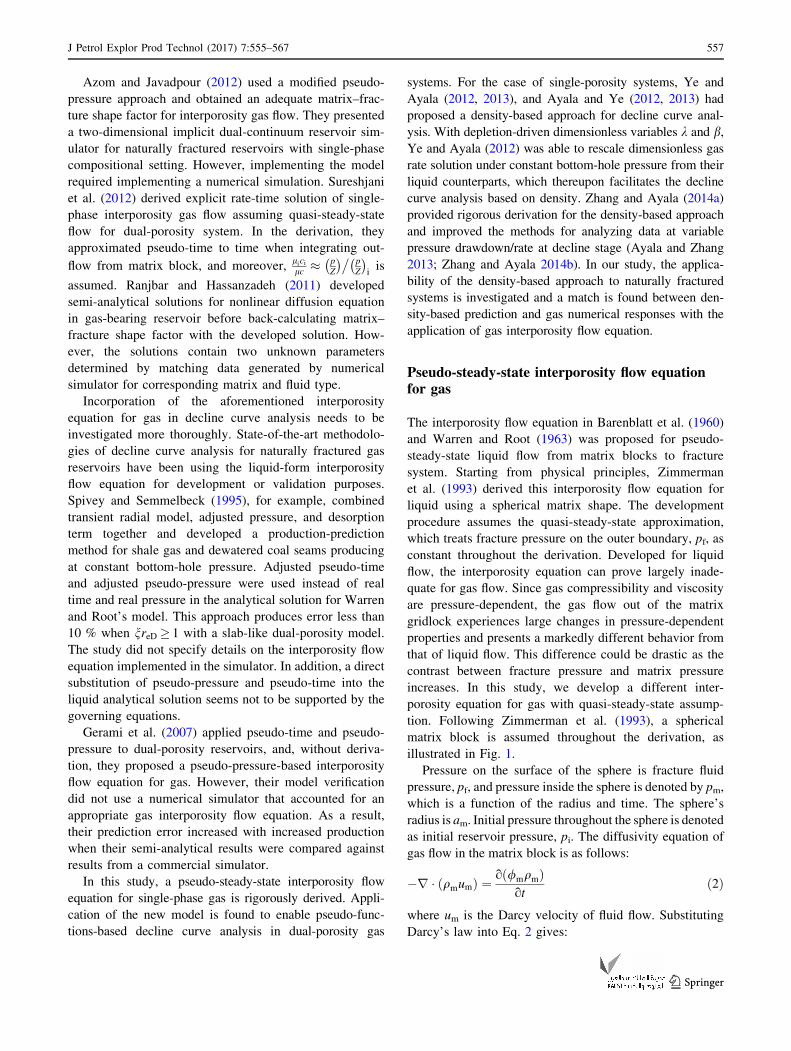
tion. Following Zimmerman et al. (1993), a spherical
matrix block is assumed throughout the derivation, as
illustrated in Fig. 1.
Pressure on the surface of the sphere is fracture fluid
pressure, pf, and pressure inside the sphere is denoted by pm,
which is a function of the radius and time. The sphere’s
radius is am. Initial pressure throughout the sphere is denoted
as initial reservoir pressure, pi. The diffusivity equation of
gas flow in the matrix block is as follows:
�r � qmumð Þ ¼ o /mqmð Þot
ð2Þ
where um is the Darcy velocity of fluid flow. Substituting
Darcy’s law into Eq. 2 gives:
J Petrol Explor Prod Technol (2017) 7:555–567 557
123
r � qmkm
lgmrpm
!¼ o /mqmð Þ
otð3Þ
Assuming an incompressible matrix rock, multiplying
both sides by h, adding the term lgmcgm=ðlgmcgmÞ on the
RHS and substituting dmðpmÞ ¼ 2hdqm=ðlgmcgmÞ gives:
r � kmrm pmð Þð Þ ¼ /mlgmcgmom pmð Þ
otð4Þ
For a homogeneous and isotropic matrix (constant km),
dividing both sides by /mlgmcgm, and substituting k�m ¼lgicgi=ðlgmcgmÞ into Eq. 4 gives:
omðpmÞk�mot
¼ km
/mlgicgir2mðpmÞ ð5Þ
Denoting �k�m as the k�m evaluated average pressure in the
matrix block and substitute b�m ¼ r �k�mdt=t into Eq. 5. This
yields:
omðpmÞo b�mt� � ¼ km
/mlgicgir2mðpmÞ ð6Þ
where b�mt is a term equivalent to normalized pseudo-time.
For gas reservoirs, the average reservoir pressure is utilized
to evaluate pseudo-time, which has been proven to work
well during boundary dominated period. Expanding Eq. 6
to spherical coordinates and taking u (r, t) = m (pm) r
gives:
ou
o b�mt� � ¼ km
/mlgicgi
o2u
or2ð7Þ
We then take the spherical matrix shape with radius am.
With the fracture surrounding the matrix, the pressure at
the matrix surface is the same as the fracture pressure. The
boundary conditions are written as:
u 0; b�mt� �
¼ 0 ð8Þ
u am; b�mt
� �¼ ammðpfÞ ð9Þ
uðr; 0Þ ¼ rmðpiÞ ð10Þ
Solving Eqs. 8–10 for mðpmÞ distribution and
calculating the average pseudo-pressure gives (Crank
1975):
mavgðpmÞ � mðpiÞmðpfÞ � mðpiÞ
¼ 1� 6
p2X1n¼1
1
n2exp � p2kmn2b
�mt
lgicgi/ma2m
!
ð11Þ
where mavg(pm) is the average pseudo-pressure throughout
the matrix block. The long-term approximation truncates to
the first term of the infinite series, giving:
mavg pmð Þ � m pið Þm pfð Þ � m pið Þ ¼ 1� 6
p2exp � p2kmb
�mt
lgicgi/ma2m
!ð12Þ
Lim and Aziz (1995) validated the long-term
approximation in their derivation for a liquid system.
This approximation is accurate for
p2kmb�mt=lgicgi/ma
2m [ 0:5 as shown in Fig. 8 of their
work. For a wide variety of cases, the approximation is
valid at the decline stage. Rearranging terms in Eq. 12
gives:
6
p2exp � p2kmb
�mt
lgicgi/ma2m
!¼ mðpfÞ � mavgðpmÞ
mðpfÞ � mðpiÞð13Þ
Taking the derivatives of Eq. 13with respect tob�mt gives:
1
mðpfÞ � mðpiÞdðmavgðpmÞÞ
d b�mt� �
¼ 6
p2exp � p2kmb
�mt
lgicgi/ma2m
!p2km
lgicgi/ma2m
ð14Þ
Writing dðmavgðpmÞÞ=d b�mt� �
in Eq. 14 asdðmavgðpmÞÞ
dtdt
d b�mtð Þ and substituting d b�mt� �
¼ �k�mdt into the
resulting equation gives:
1
mðpfÞ � m pið Þd mavg pmð Þ� �
dt
¼ 6
p2exp � p2kmb
�mt
lgicgi/ma2m
!p2km
lgicgi/ma2m
�k�m
ð15Þ
Substituting Eq. 13 into Eq. 15 gives:
dðmavgðpmÞÞ�k�mdt
¼ p2kmlgicgi/ma
2m
ðmðpfÞ � mavgðpmÞÞ ð16Þ
p2
a2mis a constant known as shape factor, a, that changes with
the geometry of matrix. Moreover, replacing average
pseudo-pressure in matrix volume, mavg(pm), with point-
Fig. 1 Schematics of a spherical matrix block
558 J Petrol Explor Prod Technol (2017) 7:555–567
123
specific matrix pseudo-pressure and substituting �k�m with
k�m since matrix is point-specific as represented by the
governing equations gives:
/m
dðmðpmÞÞk�mdt
¼ akmlgicgi
m pfð Þ � m pmð Þð Þ ð17Þ
The application of the definition of k�m and dðmðpmÞÞ ¼2hdqm=lgmcgm to Eq. 17 gives:
/m
dqmdt
¼ akm2h
ðmðpfÞ � mðpmÞÞ ð18Þ
This interporosity flow equation is rigorously derived for
gas, incorporating the viscosity–compressibility effects. An
important characteristic of this model is the same shape
factor as that in Lim and Aziz (1995) for Warren and Root’s
model. For the slab-like matrix, the shape factor is p2=4L2,where L denotes fracture half-spacing. Equation 18 is in the
same form as the interporosity flow equation written by
Gerami et al. (2007) without derivation—1 if we consider an
incompressible matrix and fracture and no connate water.
Sureshjani et al. (2012) proposed the same interporosity flow
equation in a different form with a different approach
utilizing two approximations in a different derivation:
lgicgilgcg
� p=Z
ðp=ZÞið19Þ
t � ta ð20Þ
This study shows that this pseudo-steady-state
interporosity flow equation is valid without invoking such
approximations. Sureshjani et al. (2012) built a fine grid
single-porosity numerical simulator to model flow between
slab-shaped matrix and fracture. Both the matrix and the
fracture are represented by fine gridblocks. The shape
factor is back-calculated and compared against p2=4L2,demonstrating a close match at the decline stage. The
results of the comparison validate the pseudo-steady-state
interporosity flow equation for gas. The back calculation is
thus rewritten as follows:
a ¼ 2h/m
km m pfð Þ � m pmð Þð Þdqmdt
ð21Þ
Substituting dm pmð Þ ¼ 2hdqm=lgmcgm into Eq. 18 and
canceling 2h, Eq. 18 can be rewritten as:
/m
dqmdt
¼ akm
Zqf
0
1
lgfcgfdqf �
Zqm
0
1
lgmcgmdqm
0@
1A ð22Þ
If a constant viscosity and compressibility is assumed,
Eq. 22 would collapse to the interporosity flow equation in
the Warren and Root’s model, which was developed for
liquid. Replacing lgfcgf and lgmcgm with the constant lc inEq. 22 gives:
/m
dqmdt
¼ akmlc
ðqf � qmÞ ð23Þ
The liquid systems have similar qf and qm due to small
compressibility. Thus, by substituting pf � pm ¼ln qf=qmð Þ=cl and ln(qf=qmÞ � ðqf � qmÞ=qm into Eq. 22,
the interporosity flow equation in Warren and Root’s
model is produced:
/m
1
qm
oqmot
¼ akml
pf � pmð Þ ð24Þ
The biggest obstacle to using the Warren and Root’s
model in gas scenarios is the difference between viscosity
and compressibility in the fracture systems and the matrix
systems for gas. The derived interporosity flow equation
for gas incorporates effects of pressure-dependent
properties by invoking pseudo-functions. The
development embraces pseudo-steady-state interporosity
flow and long-term approximation that requires p2kmbm* t/
lgicgi/mam2 [ 0.5 for the spherical matrix block.
Rate-time forecast of naturally fractured gasreservoirs
An in-house dual-porosity reservoir simulator, in-house
simulator 1, was developed for modeling dual-porosity gas
reservoirs using the appropriate pseudo-steady-state inter-
porosity flow equation for gas derived above. This is an
important undertaking because commercial simulators use
the liquid-form interporosity flow equation in Warren and
Root’s model with fluid properties evaluated at the pressure
of the upstream one between fracture and matrix instead.
As shown above, such liquid-version of the interporosity
equation is written as follows:
/m
oðpmÞot
¼ akmctlg
ðpf � pmÞ ð25Þ
For comparison purposes, this study also developed the
‘in-house simulator 2’, which solves all the dual-porosity
gas reservoir equations but forces the use of the liquid-
version of the interporosity equation above—as done by
commercial simulators. Our numerical simulator
implementation follows Abou-Kassem et al. (2006). A
circular reservoir is considered with a well fully penetrating
with no skin at the center. The reservoir is homogeneous and
isotropic. Logarithmic discretization is taken owing to its
radial nature. Equation discretization is implicit, and simple-
iteration method (SIM) acts as pressure advancing
algorithm. Viscosity is calculated with method by Lee
1 Per personal communication with Dr. Pooladi-Darvish where he
indicated that and they wrote it using an analogy with the liquid
formulation.
J Petrol Explor Prod Technol (2017) 7:555–567 559
123
et al. (1966). The Abou-Kassem et al. (1990) is used for
determining compressibility, and compressibility factor
calculation follows Dranchuk and Abou-Kassem (1975).
For testing purposes, a synthetic case was analyzed as
described in Tables 1 and 2. The specific gravity of natural
gas, rg, is 0.55. Matrix porosity and fracture porosity are
taken as 0.15 and 0.01, respectively. The permeability
values in the matrix and fractures are changed to 0.005 and
50 md, respectively, to guarantee apparent dual-porosity
behavior. The shape factor is assumed to be
9:98959� 10�05 1=ft2. A summary of the relevant
properties is provided in Table 1. Three scenarios with
different reservoir sizes are used for generating production
data and are presented in Table 2.
When it comes to a dual-porosity reservoirs, two sys-
tems—the fracture system and the matrix system—overlap
with each other, and the two systems communicate through
an interporosity flow described by the interporosity flow
equation. The behavior of production rate, when producing
from a dual-porosity system at constant bottom-hole pres-
sure, is different from that in a single-porosity system. As
has been pointed out by Moench (1984), in the first decline
stage, the production is primarily from fracture storage, and
matrix storage does not begin to significantly contribute to
production until the end of this stage. At the end of the first
decline stage, fluids originally in the fracture system are
depleted compared to those in the matrix system. There-
fore, with decreasing fracture fluid pressure, interporosity
flow develops and becomes dominant in the second decline
stage. That is, flow out of the matrix into the fracture makes
the dominant contribution to gas production. The matrix
blocks are therefore treated as the only storage sites at the
second decline stage, and the matrix blocks’ pressures are
representative pressure in the reservoir for evaluating
pressure-dependent effects.
For decline analysis of single-porosity gas reservoirs, Ye
and Ayala (2012, 2013) and Ayala and Ye (2012, 2013)
proposed a density-based approach. Using depletion-driven
dimensionless variables k and b, they successfully decou-
pled pressure-dependent effects from pressure depletion.
Ye and Ayala (2012) were accordingly able to show that
the dimensionless gas rate solutions under constant bottom-
hole pressure can be rescaled from their liquid counterparts
with depletion-driven dimensionless variables k and b.Zhang and Ayala (2014a) subsequently provided rigorous
derivation for the rescaling approach. The relationship is
written by Zhang and Ayala (2014a) as follows:
qgasD tDð Þ ¼ �k � qliqD �btD
� �ð26Þ
where qgasD is the dimensionless gas flow rate, q
liqD is the
liquid counterpart, and �k and �b are depletion-driven
dimensionless variables defined as follows:
�k ¼lgicgi
2h �q�qwfð Þ�m pð Þ�m pwfð Þ
ð27Þ
where �q is the average reservoir gas density, qwf is the gasdensity at the bottom-hole condition, �mðpÞ is the average
pseudo-pressure of reservoir fluids, m(pwf) is the pseudo-
pressure of gas at the bottom-hole condition, lgi and cgi are
the initial gas viscosity and initial gas compressibility,
h = RT/MW, T is temperature, and MW is molecular
weight.
b ¼R t0kdt
tð28Þ
�q could be obtained from a material balance equation
assuming a tank model for the reservoir, �m pð Þ is evaluatedat the pressure corresponding to �q. It was demonstrated that�k and �b are able to capture the effects of pressure-sensitive
properties on a single-porosity system’s behavior.
For dual-porosity reservoirs, following Moench (1984),
it would be reasonable to speculate that �k and �b could
capture the response of a dual-porosity system in the sec-
ond decline stage since the pressure-sensitive effects are
controlled by matrix pressure only. From this perspective,
the �k and �b for a dual-porosity systems could be written as�km and �bm. Considering that matrix fluids account for the
vast majority of reservoir fluids, the fracture pressure’s
influence on the average reservoir pressure is negligible.
Thus, a simple material balance equation for a single-
porosity system is able to predict the average pressure,
from which �km and �bm are then calculated.
The proposed �k and �b rescaling approach can be
validated for a variety of scenarios that exhibit dual-
porosity behaviors. First, we test the rescaling approach
against the three scenarios described by Tables 1 and 2.
The in-house simulator 1 is used to generate production
data. The rate-time production data are then transformed
into a dimensionless form and compared against rescaled
dimensionless gas production rates from analytical
dimensionless liquid flow rates.
The dimensionless flow rate produced at constant bottom-
hole pressure in a bounded circular reservoir in Laplace
space is given as follows (Da Prat et al. 1981):
~qD ¼ffiffiffiffiffiffiffiffiffiffisf sð Þ
pI1
ffiffiffiffiffiffiffiffiffiffisf sð Þ
preD
� �K1
ffiffiffiffiffiffiffiffiffiffisf sð Þ
p� �� K1
ffiffiffiffiffiffiffiffiffiffisf sð Þ
preD
� �I1
ffiffiffiffiffiffiffiffiffiffisf sð Þ
p� �� �
s I0ffiffiffiffiffiffiffiffiffiffisf sð Þ
p� �K1
ffiffiffiffiffiffiffiffiffiffisf sð Þ
preD
� �þ K0
ffiffiffiffiffiffiffiffiffiffisf sð Þ
p� �I1
ffiffiffiffiffiffiffiffiffiffisf sð Þ
preD
� �� �
ð29Þ
By numerical inversion such as the Stehfest algorithm
(Stehfest 1970) from Laplace space to real space, the
dimensionless liquid flow rate is obtained. Similar to its
counterpart in a single-porosity system (Ye and Ayala
2012), the definition of qgasD is:
560 J Petrol Explor Prod Technol (2017) 7:555–567
123
qgasD ¼
qsclgicgiqgsc2pkfh qi � qwfð Þ ð30Þ
where qsc is gas density under standard conditions and kf is
fracture permeability.
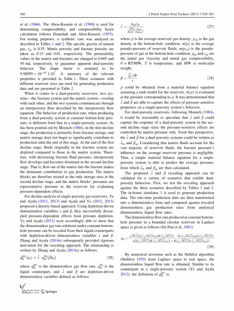
Figure 2 presents the well-known constant-pressure
liquid solutions of a dual-porosity system in terms of
qD ¼ qDðrD; tDÞ with Eq. 29 for the three different reser-
voir sizes under consideration in Tables 1 and 2 and the
rescaled liquid solutions using �km and �bm. The curves and
the dots are dimensionless liquid rates and rescaled
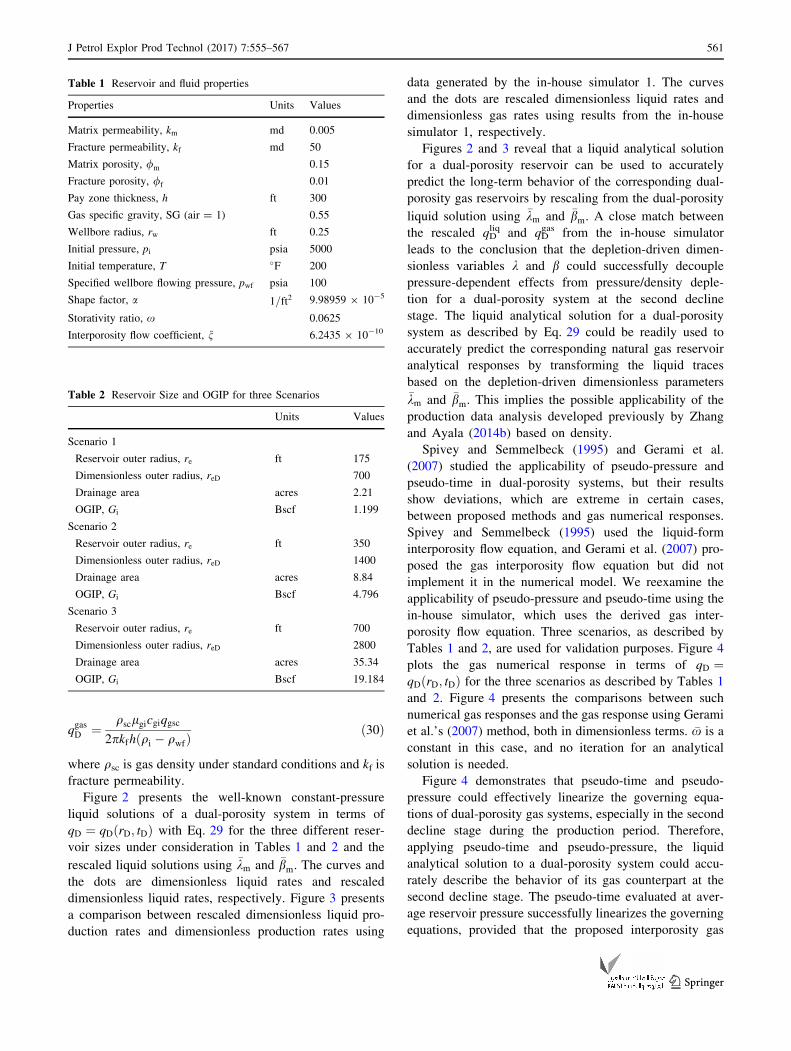
dimensionless liquid rates, respectively. Figure 3 presents
a comparison between rescaled dimensionless liquid pro-
duction rates and dimensionless production rates using
data generated by the in-house simulator 1. The curves
and the dots are rescaled dimensionless liquid rates and
dimensionless gas rates using results from the in-house
simulator 1, respectively.
Figures 2 and 3 reveal that a liquid analytical solution
for a dual-porosity reservoir can be used to accurately
predict the long-term behavior of the corresponding dual-
porosity gas reservoirs by rescaling from the dual-porosity
liquid solution using �km and �bm. A close match between
the rescaled qDliq and qD
gas from the in-house simulator
leads to the conclusion that the depletion-driven dimen-
sionless variables k and b could successfully decouple
pressure-dependent effects from pressure/density deple-
tion for a dual-porosity system at the second decline
stage. The liquid analytical solution for a dual-porosity
system as described by Eq. 29 could be readily used to
accurately predict the corresponding natural gas reservoir
analytical responses by transforming the liquid traces
based on the depletion-driven dimensionless parameters�km and �bm. This implies the possible applicability of the
production data analysis developed previously by Zhang
and Ayala (2014b) based on density.
Spivey and Semmelbeck (1995) and Gerami et al.
(2007) studied the applicability of pseudo-pressure and
pseudo-time in dual-porosity systems, but their results
show deviations, which are extreme in certain cases,
between proposed methods and gas numerical responses.
Spivey and Semmelbeck (1995) used the liquid-form
interporosity flow equation, and Gerami et al. (2007) pro-
posed the gas interporosity flow equation but did not
implement it in the numerical model. We reexamine the
applicability of pseudo-pressure and pseudo-time using the
in-house simulator, which uses the derived gas inter-
porosity flow equation. Three scenarios, as described by
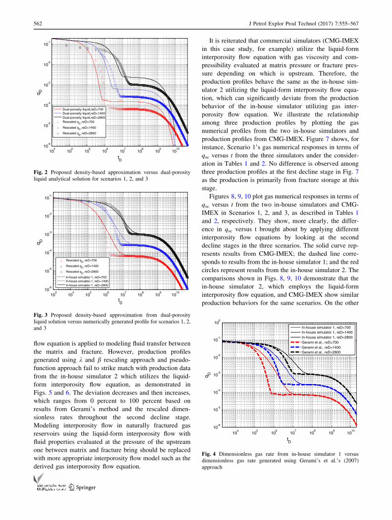
Tables 1 and 2, are used for validation purposes. Figure 4
plots the gas numerical response in terms of qD ¼qDðrD; tDÞ for the three scenarios as described by Tables 1
and 2. Figure 4 presents the comparisons between such
numerical gas responses and the gas response using Gerami
et al.’s (2007) method, both in dimensionless terms. �x is a
constant in this case, and no iteration for an analytical
solution is needed.
Figure 4 demonstrates that pseudo-time and pseudo-
pressure could effectively linearize the governing equa-
tions of dual-porosity gas systems, especially in the second
decline stage during the production period. Therefore,
applying pseudo-time and pseudo-pressure, the liquid
analytical solution to a dual-porosity system could accu-
rately describe the behavior of its gas counterpart at the
second decline stage. The pseudo-time evaluated at aver-
age reservoir pressure successfully linearizes the governing
equations, provided that the proposed interporosity gas
Table 1 Reservoir and fluid properties
Properties Units Values
Matrix permeability, km md 0.005
Fracture permeability, kf md 50
Matrix porosity, /m 0.15
Fracture porosity, /f 0.01
Pay zone thickness, h ft 300
Gas specific gravity, SG (air = 1) 0.55
Wellbore radius, rw ft 0.25
Initial pressure, pi psia 5000
Initial temperature, T �F 200
Specified wellbore flowing pressure, pwf psia 100
Shape factor, a 1=ft2 9.98959 9 10-5
Storativity ratio, x 0.0625
Interporosity flow coefficient, n 6.2435 9 10-10
Table 2 Reservoir Size and OGIP for three Scenarios
Units Values
Scenario 1
Reservoir outer radius, re ft 175
Dimensionless outer radius, reD 700
Drainage area acres 2.21
OGIP, Gi Bscf 1.199
Scenario 2
Reservoir outer radius, re ft 350
Dimensionless outer radius, reD 1400
Drainage area acres 8.84
OGIP, Gi Bscf 4.796
Scenario 3
Reservoir outer radius, re ft 700
Dimensionless outer radius, reD 2800
Drainage area acres 35.34
OGIP, Gi Bscf 19.184
J Petrol Explor Prod Technol (2017) 7:555–567 561
123
flow equation is applied to modeling fluid transfer between
the matrix and fracture. However, production profiles
generated using k and b rescaling approach and pseudo-
function approach fail to strike match with production data
from the in-house simulator 2 which utilizes the liquid-
form interporosity flow equation, as demonstrated in
Figs. 5 and 6. The deviation decreases and then increases,
which ranges from 0 percent to 100 percent based on
results from Gerami’s method and the rescaled dimen-
sionless rates throughout the second decline stage.
Modeling interporosity flow in naturally fractured gas
reservoirs using the liquid-form interporosity flow with
fluid properties evaluated at the pressure of the upstream
one between matrix and fracture bring should be replaced
with more appropriate interporosity flow model such as the
derived gas interporosity flow equation.
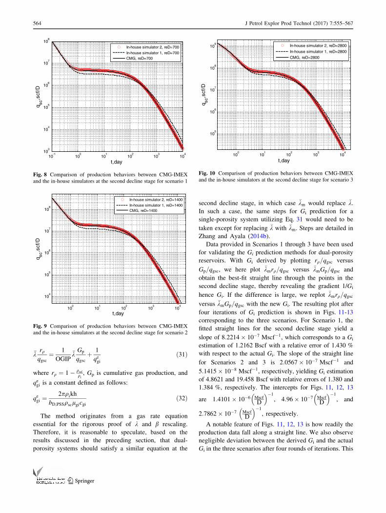
It is reiterated that commercial simulators (CMG-IMEX
in this case study, for example) utilize the liquid-form
interporosity flow equation with gas viscosity and com-
pressibility evaluated at matrix pressure or fracture pres-
sure depending on which is upstream. Therefore, the
production profiles behave the same as the in-house sim-
ulator 2 utilizing the liquid-form interporosity flow equa-
tion, which can significantly deviate from the production
behavior of the in-house simulator utilizing gas inter-
porosity flow equation. We illustrate the relationship
among three production profiles by plotting the gas
numerical profiles from the two in-house simulators and
production profiles from CMG-IMEX. Figure 7 shows, for
instance, Scenario 1’s gas numerical responses in terms of
qsc versus t from the three simulators under the consider-
ation in Tables 1 and 2. No difference is observed among
three production profiles at the first decline stage in Fig. 7
as the production is primarily from fracture storage at this
stage.
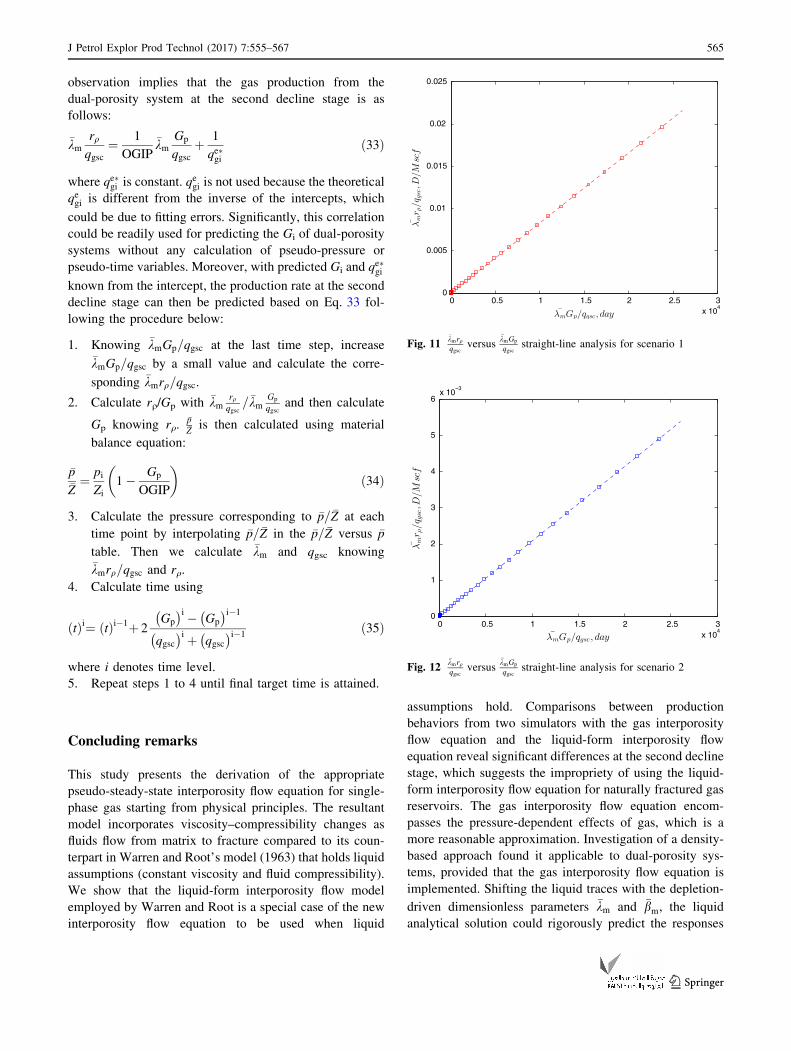
Figures 8, 9, 10 plot gas numerical responses in terms of
qsc versus t from the two in-house simulators and CMG-
IMEX in Scenarios 1, 2, and 3, as described in Tables 1
and 2, respectively. They show, more clearly, the differ-
ence in qsc versus t brought about by applying different
interporosity flow equations by looking at the second
decline stages in the three scenarios. The solid curve rep-
resents results from CMG-IMEX; the dashed line corre-
sponds to results from the in-house simulator 1; and the red
circles represent results from the in-house simulator 2. The
comparisons shown in Figs. 8, 9, 10 demonstrate that the
in-house simulator 2, which employs the liquid-form
interporosity flow equation, and CMG-IMEX show similar
production behaviors for the same scenarios. On the other
103
104
105
106
107
108
109
1010
10-6
10-5
10-4
10-3
10-2
10-1
tD
q D
Dual-porosity liquid,reD=700Dual-porosity liquid,reD=1400Dual-porosity liquid,reD=2800Rescaled q
D,reD=700
Rescaled qD
,reD=1400
Rescaled qD
,reD=2800
Fig. 2 Proposed density-based approximation versus dual-porosity
liquid analytical solution for scenarios 1, 2, and 3
103
104
105
106
107
108
109
1010
10-6
10-5
10-4
10-3
10-2
10-1
tD
q D
Rescaled qD
, reD=700
Rescaled qD
, reD=1400
Rescaled qD
, reD=2800
In-house simulator 1, reD=700In-house simulator 1, reD=1400In-house simulator 1, reD=2800
Fig. 3 Proposed density-based approximation from dual-porosity
liquid solution versus numerically generated profile for scenarios 1, 2,
and 3
104
105
106
107
108
109
1010
10-6
10-5
10-4
10-3
10-2
10-1
100
tD
q D
In-house simulator 1, reD=700In-house simulator 1, reD=1400In-house simulator 1, reD=2800Gerami et al., reD=700Gerami et al., reD=1400Gerami et al., reD=2800
Fig. 4 Dimensionless gas rate from in-house simulator 1 versus
dimensionless gas rate generated using Gerami’s et al.’s (2007)
approach
562 J Petrol Explor Prod Technol (2017) 7:555–567
123
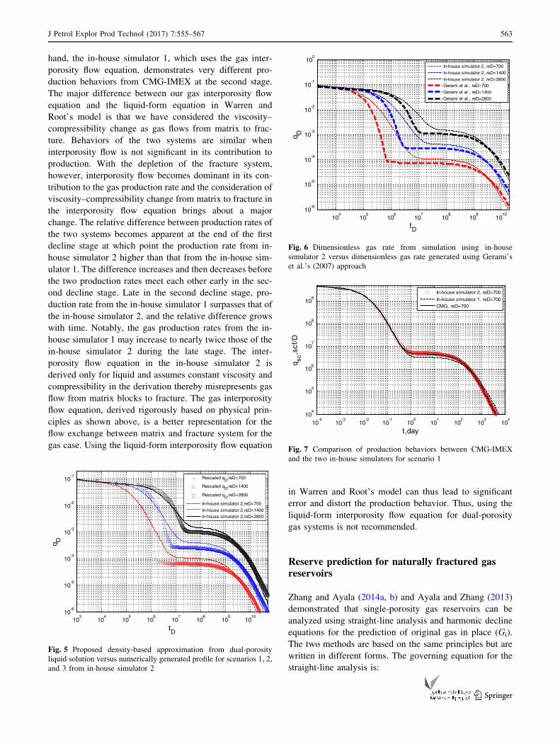
hand, the in-house simulator 1, which uses the gas inter-
porosity flow equation, demonstrates very different pro-
duction behaviors from CMG-IMEX at the second stage.
The major difference between our gas interporosity flow
equation and the liquid-form equation in Warren and
Root’s model is that we have considered the viscosity–
compressibility change as gas flows from matrix to frac-
ture. Behaviors of the two systems are similar when
interporosity flow is not significant in its contribution to
production. With the depletion of the fracture system,
however, interporosity flow becomes dominant in its con-
tribution to the gas production rate and the consideration of
viscosity–compressibility change from matrix to fracture in
the interporosity flow equation brings about a major
change. The relative difference between production rates of
the two systems becomes apparent at the end of the first
decline stage at which point the production rate from in-
house simulator 2 higher than that from the in-house sim-
ulator 1. The difference increases and then decreases before
the two production rates meet each other early in the sec-
ond decline stage. Late in the second decline stage, pro-
duction rate from the in-house simulator 1 surpasses that of
the in-house simulator 2, and the relative difference grows
with time. Notably, the gas production rates from the in-
house simulator 1 may increase to nearly twice those of the
in-house simulator 2 during the late stage. The inter-
porosity flow equation in the in-house simulator 2 is
derived only for liquid and assumes constant viscosity and
compressibility in the derivation thereby misrepresents gas
flow from matrix blocks to fracture. The gas interporosity
flow equation, derived rigorously based on physical prin-
ciples as shown above, is a better representation for the
flow exchange between matrix and fracture system for the
gas case. Using the liquid-form interporosity flow equation
in Warren and Root’s model can thus lead to significant
error and distort the production behavior. Thus, using the
liquid-form interporosity flow equation for dual-porosity
gas systems is not recommended.
Reserve prediction for naturally fractured gasreservoirs
Zhang and Ayala (2014a, b) and Ayala and Zhang (2013)
demonstrated that single-porosity gas reservoirs can be
analyzed using straight-line analysis and harmonic decline
equations for the prediction of original gas in place (Gi).
The two methods are based on the same principles but are
written in different forms. The governing equation for the
straight-line analysis is:
103
104
105
106
107
108
109
1010
10-6
10-5
10-4
10-3
10-2
10-1
tD
q D
Rescaled qD,reD=700
Rescaled qD,reD=1400
Rescaled qD,reD=2800
In-house simulator 2,reD=700
In-house simulator 2,reD=1400In-house simulator 2,reD=2800
Fig. 5 Proposed density-based approximation from dual-porosity
liquid solution versus numerically generated profile for scenarios 1, 2,
and 3 from in-house simulator 2
104
105
106
107
108
109
1010
10-6
10-5
10-4
10-3
10-2
10-1
100
tD
q D
In-house simulator 2, reD=700
In-house simulator 2, reD=1400
In-house simulator 2, reD=2800Gerami et al., reD=700
Gerami et al., reD=1400
Gerami et al., reD=2800
Fig. 6 Dimensionless gas rate from simulation using in-house
simulator 2 versus dimensionless gas rate generated using Gerami’s
et al.’s (2007) approach
10-4
10-3
10-2
10-1
100
101
102
103
104
104
105
106
107
108
109
t,day
q sc,s
cf/D
In-house simulator 2, reD=700
In-house simulator 1, reD=700CMG, reD=700
Fig. 7 Comparison of production behaviors between CMG-IMEX
and the two in-house simulators for scenario 1
J Petrol Explor Prod Technol (2017) 7:555–567 563
123
�krq
qgsc¼ 1
OGIP�kGp
qgscþ 1
qegið31Þ
where rq ¼ 1� qwfqi, Gp is cumulative gas production, and
qegi is a constant defined as follows:
qegi ¼2pqikh
bD;PSSqsclgicgið32Þ
The method originates from a gas rate equation
essential for the rigorous proof of k and b rescaling.
Therefore, it is reasonable to speculate, based on the
results discussed in the preceding section, that dual-
porosity systems should satisfy a similar equation at the
second decline stage, in which case �km would replace �k.In such a case, the same steps for Gi prediction for a
single-porosity system utilizing Eq. 31 would need to be
taken except for replacing �k with �km. Steps are detailed in
Zhang and Ayala (2014b).
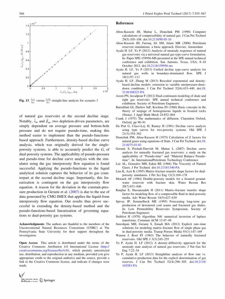
Data provided in Scenarios 1 through 3 have been used
for validating the Gi prediction methods for dual-porosity
reservoirs. With Gi derived by plotting rq=qgsc versus
Gp=qgsc, we here plot �kmrq=qgsc versus �kmGp=qgsc and
obtain the best-fit straight line through the points in the
second decline stage, thereby revealing the gradient 1/Gi
hence Gi. If the difference is large, we replot �kmrq=qgscversus �kmGp=qgsc with the new Gi. The resulting plot after
four iterations of Gi prediction is shown in Figs. 11-13
corresponding to the three scenarios. For Scenario 1, the
fitted straight lines for the second decline stage yield a
slope of 8:2214� 10�7 Mscf�1, which corresponds to a Gi
estimation of 1.2162 Bscf with a relative error of 1.430 %
with respect to the actual Gi. The slope of the straight line
for Scenarios 2 and 3 is 2:0567� 10�7 Mscf�1 and
5:1415� 10�8 Mscf�1, respectively, yielding Gi estimation
of 4.8621 and 19.458 Bscf with relative errors of 1.380 and
1.384 %, respectively. The intercepts for Figs. 11, 12, 13
are 1:4101� 10�6 Mscf
D
� ��1
, 4:96� 10�7 Mscf
D
� ��1
, and
2:7862� 10�7 Mscf
D
� ��1
, respectively.
A notable feature of Figs. 11, 12, 13 is how readily the
production data fall along a straight line. We also observe
negligible deviation between the derived Gi and the actual
Gi in the three scenarios after four rounds of iterations. This
10-1
100
101
102
103
104
103
104
105
106
107
108
t,day
q sc,s
cf/D
In-house simulator 2, reD=700
In-house simulator 1, reD=700CMG, reD=700
Fig. 8 Comparison of production behaviors between CMG-IMEX
and the in-house simulators at the second decline stage for scenario 1
100
101
102
103
104
104
105
106
107
108
t,day
q sc,s
cf/D
In-house simulator 2, reD=1400
In-house simulator 1, reD=1400CMG, reD=1400
Fig. 9 Comparison of production behaviors between CMG-IMEX
and the in-house simulators at the second decline stage for scenario 2
100
101
102
103
104
105
106
107
108
109
t,day
q sc,s
cf/D
In-house simulator 2, reD=2800
In-house simulator 1, reD=2800
CMG, reD=2800
Fig. 10 Comparison of production behaviors between CMG-IMEX
and the in-house simulators at the second decline stage for scenario 3
564 J Petrol Explor Prod Technol (2017) 7:555–567
123
observation implies that the gas production from the
dual-porosity system at the second decline stage is as
follows:
�kmrq
qgsc¼ 1
OGIP�km
Gp
qgscþ 1
qe�gið33Þ
where qe�gi is constant. qegi is not used because the theoretical
qegi is different from the inverse of the intercepts, which
could be due to fitting errors. Significantly, this correlation
could be readily used for predicting the Gi of dual-porosity
systems without any calculation of pseudo-pressure or
pseudo-time variables. Moreover, with predicted Gi and qe�gi
known from the intercept, the production rate at the second
decline stage can then be predicted based on Eq. 33 fol-
lowing the procedure below:
1. Knowing �kmGp=qgsc at the last time step, increase�kmGp=qgsc by a small value and calculate the corre-
sponding �kmrq=qgsc.
2. Calculate rq/Gp with �kmrqqgsc
=�kmGp
qgscand then calculate
Gp knowing rq.�p�Zis then calculated using material
balance equation:
�p�Z¼ pi
Zi1� Gp
OGIP
� ð34Þ
3. Calculate the pressure corresponding to �p=�Z at each
time point by interpolating �p=�Z in the �p=�Z versus �p
table. Then we calculate �km and qgsc knowing�kmrq=qgsc and rq.
4. Calculate time using
tð Þi¼ tð Þi�1þ 2Gp
� �i � Gp
� �i�1
qgsc� �i þ qgsc
� �i�1ð35Þ
where i denotes time level.
5. Repeat steps 1 to 4 until final target time is attained.
Concluding remarks
This study presents the derivation of the appropriate
pseudo-steady-state interporosity flow equation for single-
phase gas starting from physical principles. The resultant
model incorporates viscosity–compressibility changes as
fluids flow from matrix to fracture compared to its coun-
terpart in Warren and Root’s model (1963) that holds liquid
assumptions (constant viscosity and fluid compressibility).
We show that the liquid-form interporosity flow model
employed by Warren and Root is a special case of the new
interporosity flow equation to be used when liquid
assumptions hold. Comparisons between production
behaviors from two simulators with the gas interporosity
flow equation and the liquid-form interporosity flow
equation reveal significant differences at the second decline
stage, which suggests the impropriety of using the liquid-
form interporosity flow equation for naturally fractured gas
reservoirs. The gas interporosity flow equation encom-
passes the pressure-dependent effects of gas, which is a
more reasonable approximation. Investigation of a density-
based approach found it applicable to dual-porosity sys-
tems, provided that the gas interporosity flow equation is
implemented. Shifting the liquid traces with the depletion-
driven dimensionless parameters �km and �bm, the liquid
analytical solution could rigorously predict the responses
0 0.5 1 1.5 2 2.5 3x 10
4
0
0.005
0.01
0.015
0.02
0.025
Fig. 11�kmrqqgsc
versus�kmGp
qgscstraight-line analysis for scenario 1
0 0.5 1 1.5 2 2.5 3x 10
4
0
1
2
3
4
5
6x 10
−3
Fig. 12�kmrqqgsc
versus�kmGp
qgscstraight-line analysis for scenario 2
J Petrol Explor Prod Technol (2017) 7:555–567 565
123
of natural gas reservoirs at the second decline stage.
Notably, �km and �bm, two depletion-driven parameters, are
simply dependent on average pressure and bottom-hole
pressure and do not require pseudo-time, making this
method easier to implement than the pseudo-functions-
based approach. Furthermore, density-based decline curve
analysis, which was originally derived for the single-
porosity systems, is able to accurately predict the Gi of
dual-porosity systems. The applicability of pseudo-pressure
and pseudo-time for decline curve analysis with the sim-
ulator using the gas interporosity flow equation is found
successful. Applying the pseudo-functions to the liquid
analytical solution captures the behavior of its gas coun-
terpart at the second decline stage. Importantly, this lin-
earization is contingent on the gas interporosity flow
equation. A reason for the deviation in the constant-pres-
sure production in Gerami et al. (2007) is due to the use of
data generated by CMG-IMEX that applies the liquid-form
interporosity flow equation. Our results thus prove suc-
cessful in extending the density-based method and the
pseudo-functions-based linearization of governing equa-
tions to dual-porosity gas systems.
Acknowledgments The authors are thankful to the members of the
Unconventional Natural Resources Consortium (UNRC) at The
Pennsylvania State University for their support throughout the
investigation.
Open Access This article is distributed under the terms of the
Creative Commons Attribution 4.0 International License (http://
creativecommons.org/licenses/by/4.0/), which permits unrestricted
use, distribution, and reproduction in any medium, provided you give
appropriate credit to the original author(s) and the source, provide a
link to the Creative Commons license, and indicate if changes were
made.
References
Abou-Kassem JH, Mattar L, Dranchuk PM (1990) Computer
calculations of compressibility of natural gas. J Can Pet Technol
29(5):105–108. doi:10.2118/90-05-10
Abou-Kassem JH, Farouq Ali SM, Islam MR (2006) Petroleum
reservoir simulations: a basic approach. Elsevier, Amsterdam
Ayala H. LF, Ye P (2012) Analysis of unsteady responses of natural
gas reservoirs via a universal natural gas type-curve formulation.
In: Paper SPE-159956-MS presented at the SPE annual technical
conference and exhibition. San Antonio, Texas, USA, 8–10
October 2012. doi:10.2118/159956-ms
Ayala H. LF, Ye P (2013) Unified decline type-curve analysis for
natural gas wells in boundary-dominated flow. SPE J
18(1):97–113
Ayala H. LF, Zhang M (2013) Rescaled exponential and density-
based decline models: extension to variable rate/pressure-draw-
down conditions. J Can Pet Technol 52(6):433–440. doi:10.
2118/168223-PA
Azom PN, Javadpour F (2012) Dual-continuum modeling of shale and
tight gas reservoirs. SPE annual technical conference and
exhibition. Society of Petroleum Engineers.
Barenblatt GI, Zheltov IuP, Kochina IN (1960) Basic concepts in the
theory of seepage of homogeneous liquids in fissured rocks
(Strata). J Appl Math Mech 24:852–864
Crank J (1975) The mathematics of diffusion. Clarendon Oxford,
Oxford, pp 90–91
Da Prat G, Cinco-Ley H, Ramey H (1981) Decline curve analysis
using type curves for two-porosity systems. Old SPE J
21(3):354–362
Dranchuk PM, Abou-Kassem H (1975) Calculation of Z factors for
natural gases using equations of State. J Can Pet Technol. doi:10.
2118/75-03-03
Gerami S, Pooladi-Darvish M, Mattar L (2007) Decline curve
analysis for naturally fractured gas reservoirs: a study on the
applicability of ‘‘Pseudo-time’’ and ‘‘Material Balance Pseudo-
time’’. In: InternationalPetroleum Technology Conference
Lee AL, Gonzalez MH, Eakin BE (1966) The Viscosity of Natural
Gases. J Pet Technol. doi:10.2118/1340-PA
Lim K, Aziz K (1995) Matrix-fracture transfer shape factors for dual-
porosity simulators. J Pet Sci Eng 13(3):169–178
Moench AF (1984) Double-porosity models for a fissured ground-
water reservoir with fracture skin. Water Resour Res
20(7):831–846
Ranjbar E, Hassanzadeh H (2011) Matrix–fracture transfer shape
factor for modeling flow of a compressible fluid in dual-porosity
media. Adv Water Resour 34(5):627–639
Spivey JP, Semmelbeck ME (1995) Forecasting long-term gas
production of dewatered coal seams and fractured gas shales.
In: Low Permeability Reservoirs Symposium, Society of
Petroleum Engineers
Stehfest H (1970) Algorithm 368: numerical inversion of laplace
transforms. Commun ACM 13:47–49
Sureshjani MH, Gerami S, Emadi MA (2012) Explicit rate–time
solutions for modeling matrix–fracture flow of single phase gas
in dual-porosity media. Transp Porous Media 93(1):147–169
Warren J, Root PJ (1963) The behavior of naturally fractured
reservoirs. Old SPE J 3(3):245–255
Ye P, Ayala H. LF (2012) A density-diffusivity approach for the
unsteady state analysis of natural gas reservoirs. J Nat Gas Sci
Eng 7:22–34
Ye P, Ayala H. LF (2013) Straightline analysis of flow rate vs.
cumulative-production data for the explicit determination of gas
reserves. J Can Pet Technol 52(4):296–305. doi:10.2118/
165583-PA
0 0.5 1 1.5 2 2.5 3x 10
4
0
0.2
0.4
0.6
0.8
1
1.2
1.4x 10
−3
Fig. 13�kmrqqgsc
versus�kmGp
qgscstraight-line analysis for scenario 3
566 J Petrol Explor Prod Technol (2017) 7:555–567
123
Zhang M, Ayala H. LF (2014a) Gas-rate forecasting in boundary-
dominated flow: constant-bottomhole-pressure decline analysis
by use of rescaled exponential models. SPE J 19(3):410–417.
doi:10.2118/168217-PA
Zhang M, Ayala H. LF (2014b) Gas-production-data analysis of
variable-pressure-drawdown/variable-rate systems: a density-
based approach. SPE Reserv Eval Eng 17(4):520–529. doi:10.
2118/172503-PA
Zimmerman RW, Chen G, Hadgu T, Bodvarsson GS (1993) A
numerical dual-porosity model with semianalytical treatment of
fracture/matrix flow. Water Resour Res 29(7):2127–2137
J Petrol Explor Prod Technol (2017) 7:555–567 567
123