datalogging - pdst · datalogging allows real-time data such as ... advisable to connect your...

Datalogging

Datalogging and Datalogging Activities Page

What is datalogging 2

Datalogging activities 5

PASCO

a. Investigate the effect of exercise on the pulse rate of a human 6

b. Conduct any activity to demonstrate osmosis 10

c. Effect of pH on the rate of catalase activity 13

d. Prepare and show the production of alcohol by yeast 16

e. Investigate the abiotic factor, pH, in an ecosystem 19

VERNIER

a. Investigate the effect of exercise on the pulse rate of a human 23

b. Conduct any activity to demonstrate osmosis 26

c. Effect of pH on the rate of catalase activity 28

d. Prepare and show the production of alcohol by yeast 30

e. Investigate the abiotic factor, pH, in an ecosystem 32

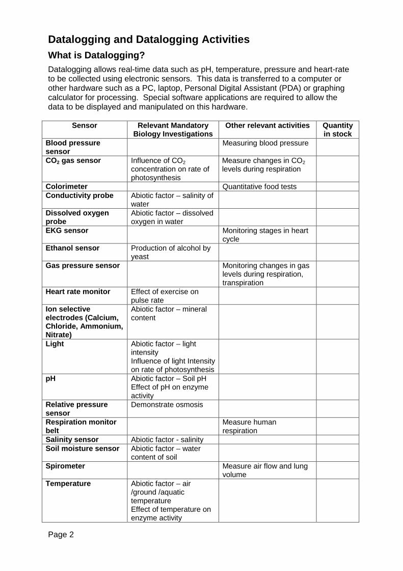
Datalogging and Datalogging Activities What is Datalogging? Datalogging allows real-time data such as pH, temperature, pressure and heart-rate to be collected using electronic sensors. This data is transferred to a computer or other hardware such as a PC, laptop, Personal Digital Assistant (PDA) or graphing calculator for processing. Special software applications are required to allow the data to be displayed and manipulated on this hardware.

Sensor Relevant Mandatory

Biology Investigations Other relevant activities Quantity

in stock Blood pressure sensor

Measuring blood pressure

CO2 gas sensor Influence of CO2 concentration on rate of photosynthesis

Measure changes in CO2 levels during respiration

Colorimeter Quantitative food tests Conductivity probe Abiotic factor – salinity of

water

Dissolved oxygen probe

Abiotic factor – dissolved oxygen in water

EKG sensor Monitoring stages in heart cycle

Ethanol sensor Production of alcohol by yeast

Gas pressure sensor Monitoring changes in gas levels during respiration, transpiration

Heart rate monitor Effect of exercise on pulse rate

Ion selective electrodes (Calcium, Chloride, Ammonium, Nitrate)

Abiotic factor – mineral content

Light Abiotic factor – light intensity Influence of light Intensity on rate of photosynthesis

pH Abiotic factor – Soil pH Effect of pH on enzyme activity

Relative pressure sensor

Demonstrate osmosis

Respiration monitor belt

Measure human respiration

Salinity sensor Abiotic factor - salinity Soil moisture sensor Abiotic factor – water

content of soil

Spirometer Measure air flow and lung volume

Temperature Abiotic factor – air /ground /aquatic temperature Effect of temperature on enzyme activity

Components of a basic Datalogging system Every datalogging system has the following main components:

1. Sensor e.g. light, temperature 2. Interface: transfers data collected from the sensor to the computer/hardware. 3. Computer/Hardware: stores and displays the collected data. 4. Software: allows computer to interpret the data collected.

Sensors More than fifty types of sensor are available from different companies. Some of those most popular for Biology include; CO2 gas sensor, light sensor, pressure sensor, dissolved oxygen probe, heart-rate monitor, pH sensor, temperature probe, anemometer sensor and water quality sensors. A practical tip when using sensors is to clamp the probe so that it dips into what you are measuring. This reduces the risk of equipment being knocked over. Finally, it is advisable to connect your sensors to the datalogger and computer before starting the software. Interface There are two main types of interfaces that may be used to connect the sensors to the computer. The first and least expensive provides a simple route from the sensor to the computer/hardware and allows you to display the results ‘live’. The second kind, a datalogger, can store and record readings which can later be transferred to the computer. This facility allows remote data-collection for example when carrying out fieldwork. Dataloggers are either fitted with a rechargeable internal battery or employ regular alkaline batteries. It is advisable when storing such dataloggers that the batteries be removed when not in use to prolong their lifespan. Some may also have an external power supply. Normally such dataloggers may be connected to a computer by a cable. Up to four sensors may be connected to some interfaces. Thus, more than one parameter may be monitored at a time. Computer/Hardware Every datalogging system requires hardware such as PCs, laptops, graphing calculators or PDAs. When choosing which hardware system to employ, consideration should be given to the following;

• PCs and laptops are more appropriate for whole class demonstration and may be connected to a data-projector to display data and graphs to a class.

• The majority of operating systems support datalogging hardware and software but this should be checked with the datalogging manufacturer.

• Hard drives, floppy discs and USB pen drives may be used to store data. • PDAs that offer colour display and sound are a more expensive option but are

less robust than graphing calculators.

Software In addition to recording data from sensors, datalogging software allows the data to be manipulated in various ways. Data may be displayed in various forms such as time graphs, digital meters or bar gauges. A crucial feature is being able to change the scale of a graph to zoom in on interesting sections. In addition, being able to correlate a graph to a table of results is very useful. Statistical features allow minimum, maximum and average values to be calculated, in addition to the area under a graph or the slope of a graph. Furthermore, curve fitting

allows you to choose from a list of functions or curves and see which best fits the data. It is also possible to carry out all these functions on a selected region of a graph. Graphs may also be formatted in various ways such as adding titles, labels or comments. Advantages of using datalogging

• Accurate ‘real time’ data may be collected. • Stored data is easily manipulated and graphed using software. • Two or more parameters e.g. light intensity and temperature may be monitored

at once. • Allows students to focus on higher order thinking skills such as data analysis,

interpretation of graphs, result prediction and reflecting on the control of variables.

• Allows measurements to be taken over long periods of time e.g. overnight. • Investigations may be repeated easily in a short period of time. • Promotes student motivation. • Promotes collaborative work between students. • Remote data collection e.g. fieldwork may be carried out.

Purchasing considerations When choosing which datalogging system to purchase, consideration should be given to the following;

• Sensors are generally not easily exchanged between systems; therefore, it is advisable to check which sensors are available for use with the datalogger.

• Some sensors may be expensive. It is advisable to start with a small number of each type of sensor and scale up according to interests.

Commercial websites: www.casio.co.uk www.data-harvest.com www.dcpmicro.com www.economatics.co.uk www.education.ti.com www.pasco.com www.philipharris.co.uk www.picotech.com www.r-p-r.co.uk/ www.vernier.co

http://www.casio.co.uk/

http://www.data-harvest.com/

http://www.dcpmicro.com/

http://www.economatics.co.uk/

http://www.education.ti.com/

http://www.pasco.com/

http://www.philipharris.co.uk/

http://www.picotech.com/

http://www.r-p-r.co.uk/

Datalogging activities PASCO

And now ……..

PASCO Software

USB link

PasPort Xplorer

PasPort GLX

500 interface

750 interface

Computer based

Remote logging

Graphical analysis

PASCO Interfaces

The SPARK Science Learning

System

Media rich, touch screen capable and with powerful analysis tools

SPARKvue For

iPhone

Touchscreen

(a) Investigate the effect of exercise on the pulse rate of a human Background The Exercise Heart Rate Sensor uses a chest transmitter belt and a sensor (receiver) to measure heart rates (pulse rates) between 40 and 240 beats per minute. Basic procedure (PasPort interface)

1. Connect the USB link to a USB port on your computer. 2. Moisten the belt and wrap it around your chest or hold it in both hands. 3. Connect the sensor to the USB link. 4. The software automatically launches when it detects a PasPort sensor. 5. From the PasPortal window, select launch DataStudio 6. A graph of Heart Rate against Time appears. 7. Place the sensor on a table. (Continue to step 8 …)

Basic procedure (Science Workshop interface)

Connect the Science Workshop 500 interface to the serial port of the computer using the serial lead provided. Switch the interface to ‘ON’

or Connect the Science Workshop 500 interface to the USB port of the laptop using the USB/serial converter lead provided. Switch the interface to ‘ON’ 1. Connect the sensor to channel A on the interface. Close the window. 2. Double click on the DataStudio icon on the desktop. 3. Select Create Experiment. 4. From the Sensors list on the L.H.S. double-click on heart rate sensor to connect this

sensor to channel A on the interface. 5. Under on the L.H.S. double click on graph to create a graph display. 6. From Choose a Data Source select heart rate and click OK. A graph display of Heart

Rate vs Time appears. 7. Sit comfortably on a chair. 8. On the main toolbar, click the button and record your resting heart rate for 60

seconds. 9. Click the button to stop collecting data 10. Select the button. 11. Use the button to display max, min and mean heart rates. 12. Begin walking briskly 13. Repeat steps 8 to 10. 14. Begin running 15. Repeat steps 8 to 10.

Skill builders

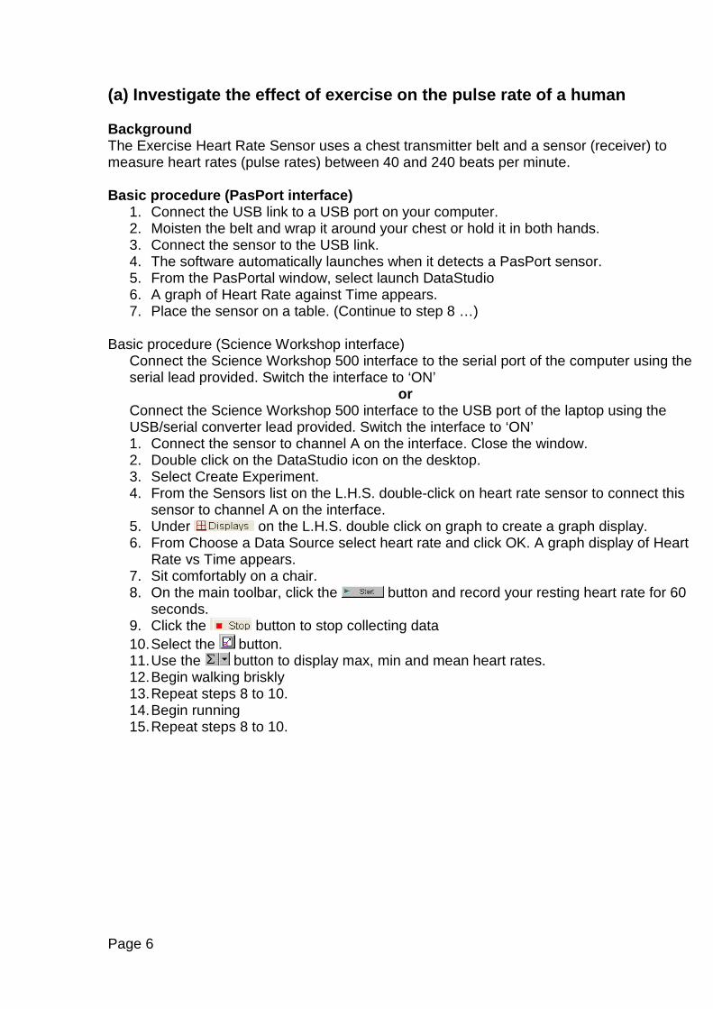
⇒ Saving your file 1. From the toolbar go to File and Save Activity As …

2. Navigate to the folder in which you wish to store your file Give the file a name followed by Save.

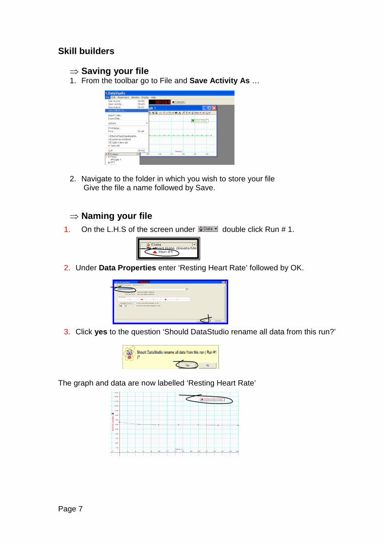
⇒ Naming your file 1. On the L.H.S of the screen under double click Run # 1.

2. Under Data Properties enter ‘Resting Heart Rate’ followed by OK.

3. Click yes to the question ‘Should DataStudio rename all data from this run?’

The graph and data are now labelled ‘Resting Heart Rate’

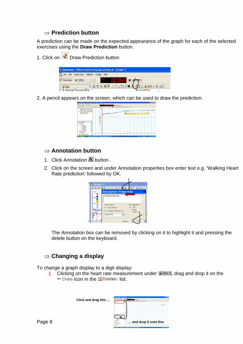
⇒ Prediction button A prediction can be made on the expected appearance of the graph for each of the selected exercises using the Draw Prediction button.

1. Click on Draw Prediction button 2. A pencil appears on the screen, which can be used to draw the prediction.

⇒ Annotation button 1. Click Annotation button. 2. Click on the screen and under Annotation properties box enter text e.g. ‘Walking Heart

Rate prediction’ followed by OK.

The Annotation box can be removed by clicking on it to highlight it and pressing the delete button on the keyboard.

⇒ Changing a display

To change a graph display to a digit display:

1. Clicking on the heart rate measurement under , drag and drop it on the icon in the list.

Click and drag this …

… and drop it onto this

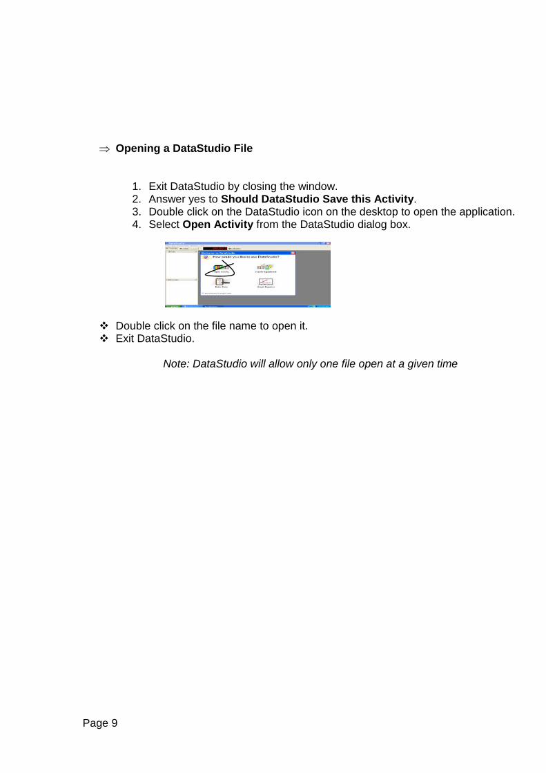
⇒ Opening a DataStudio File

1. Exit DataStudio by closing the window. 2. Answer yes to Should DataStudio Save this Activity. 3. Double click on the DataStudio icon on the desktop to open the application. 4. Select Open Activity from the DataStudio dialog box.

Double click on the file name to open it. Exit DataStudio.

Note: DataStudio will allow only one file open at a given time

(b) Conduct any experiment to demonstrate Osmosis

Background A relative pressure sensor is used to measure pressure in kilopascals (kPa), psi, or N/m2. As water moves by osmosis through the dialysis tubing the change in pressure is detected by the relative pressure sensor. Basic Procedure (PasPort interface)

1. Attach a rubber bung and connecting tube to the PasPort relative pressure sensor

2. Connect the USB link using the USB cable to a USB port on the computer.

3. Connect the PasPort relative pressure sensor to the USB link. 4. The software automatically launches when it detects the PasPort sensor. 5. From the PasPortal window select launch DataStudio. 6. A graph of Relative Pressure against Time appears.

Basic procedure (Science Workshop interface) Connect the Science Workshop 500 interface to the serial port of the computer using the serial lead provided. Switch the interface to ‘ON’

or Connect the Science Workshop 500 interface to the USB port of the laptop using the USB/Serial converter lead provided. Switch the interface to ‘ON’ 1. Double click on the DataStudio icon on the desktop. 2. Select Create Experiment. 3. From the Sensors list on the L.H.S. double-click on pressure sensor to connect this

sensor to Channel A on the interface. 4. Under on the L.H.S. double click on graph to create a graph display. 5. From Choose a Data Source select Pressure and click OK. A graph display of Pressure

vs Time appears. Experimental procedure 1. Soften two 20 cm strips of dialysis tubing by soaking them in

water. 2. Tie a knot at one end of each strip. 3. About half-fill one piece of tubing with sucrose solution and

the other with distilled water. 4. Eliminate as much air as possible from the tubing with the

sucrose solution. 5. Wash off any excess sucrose solution from the outside of

the sucrose tubing and pat dry both tubing with the paper towels.

6. Connect the relative pressure sensor to the open end of the tubing. Draw the tubing up around the rubber bung ensuring an air tight fit.

7. Suspend the tubing containing the concentrated sucrose solution, in a beaker of distilled water.

8. On the main toolbar, click the button to start collecting data 9. Select the Scale to Fit button.

10. The datalogger collects and graphs the data. 11. After the selected time has passed click the stop button. 12. Remove the Relative Pressure sensor from the conical flask. A graph labelled Run # 1 has been completed on the screen. 13. Repeat steps 4 -11 for tube labelled ‘distilled water’. This acts as a control.

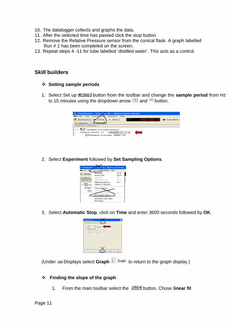
Skill builders Setting sample periods 1. Select Set up button from the toolbar and change the sample period from Hz

to 15 minutes using the dropdown arrow and button.

2. Select Experiment followed by Set Sampling Options.

3. Select Automatic Stop, click on Time and enter 3600 seconds followed by OK.

(Under Displays select Graph to return to the graph display.) Finding the slope of the graph

1. From the main toolbar select the button. Chose linear fit

2. Highlight the data points of interest by clicking and dragging around the relevant data points until they are highlighted in yellow.

3. Read and record the value for slope e.g. 0.0025.This data represents the rate of osmosis

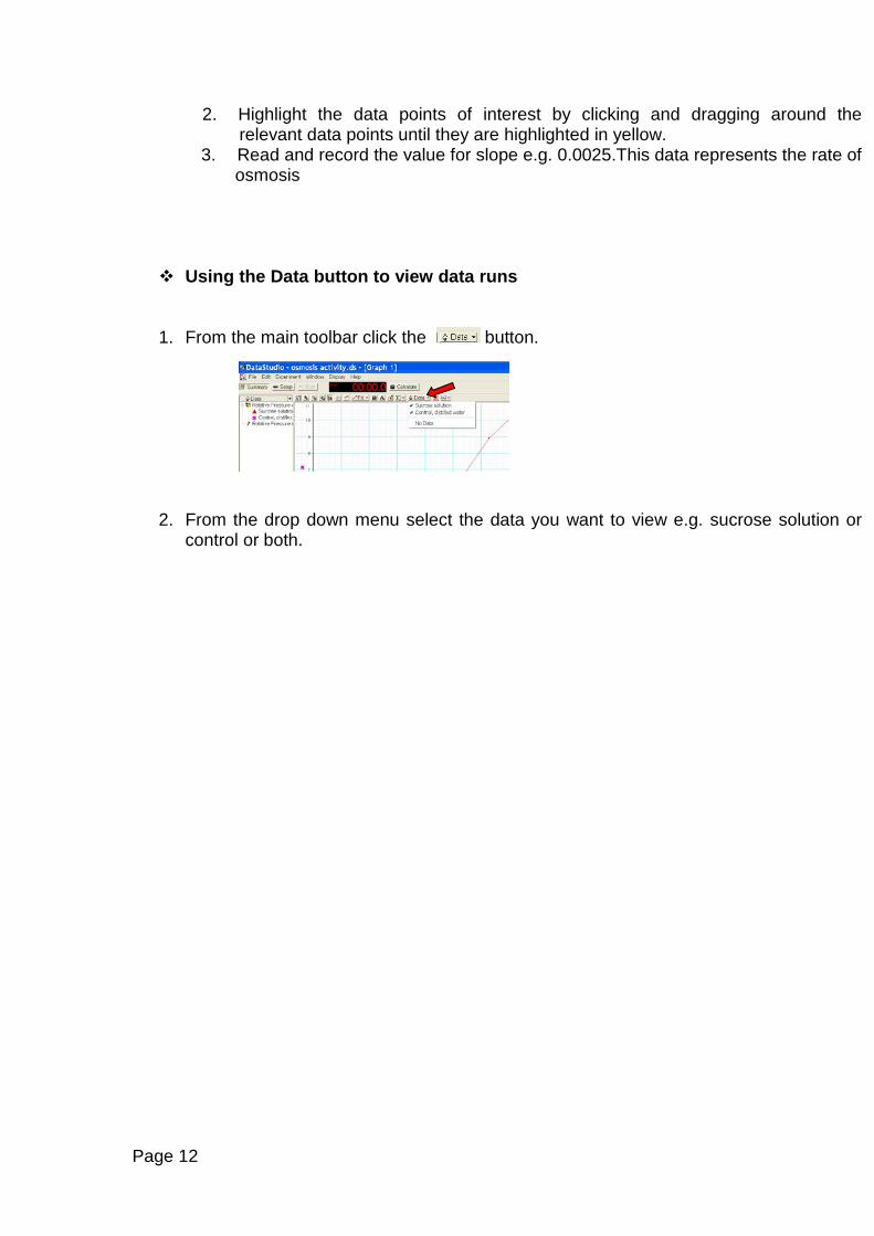
Using the Data button to view data runs 1. From the main toolbar click the button.

2. From the drop down menu select the data you want to view e.g. sucrose solution or

control or both.

(c) Effect of pH on the rate of catalase activity

The absolute pressure sensor measures pressure in kilopascals (kPa), psi, or N/m2. A graph of the rate of enzyme activity vs pH is required. This activity is carried out in two stages: A graph of pressure vs time is prepared for each pH

value. The slopes of these graphs represent the rate of enzyme activity. A graph of pH against the rate of enzyme activity is

then prepared. Basic procedure (PasPort interface)

1. Attach a rubber bung and connecting tube to the PasPort absolute pressure sensor. 2. Connect the USB link using the USB cable to a USB port on the computer. 3. Connect the PasPort absolute pressure sensor to the USB link. 4. The software automatically launches enzyme activity when it detects the PasPort

sensor. 5. From the PasPortal window select launch DataStudio.

Basic procedure (ScienceWorkshop interface)

• Connect the Science Workshop 500 interface to the serial port of the computer using the serial lead provided. Switch the interface to ‘ON’.

or 2. Connect the Science Workshop 500 interface to the USB port of the laptop using the USB/Serial converter lead provided. Switch the interface to ‘ON’. • Double click on the DataStudio icon on the desktop. • Select Create Experiment. • From the Sensors list on the L.H.S. double-click on pressure sensor to connect this

sensor to channel A on the interface. • Under on the L.H.S. double click on graph to create a graph display. • From Choose a Data Source select pressure and click OK. A graph display of

Pressure vs Time appears. • Set sample period to 1 second. • Set automatic stop to 300 seconds.

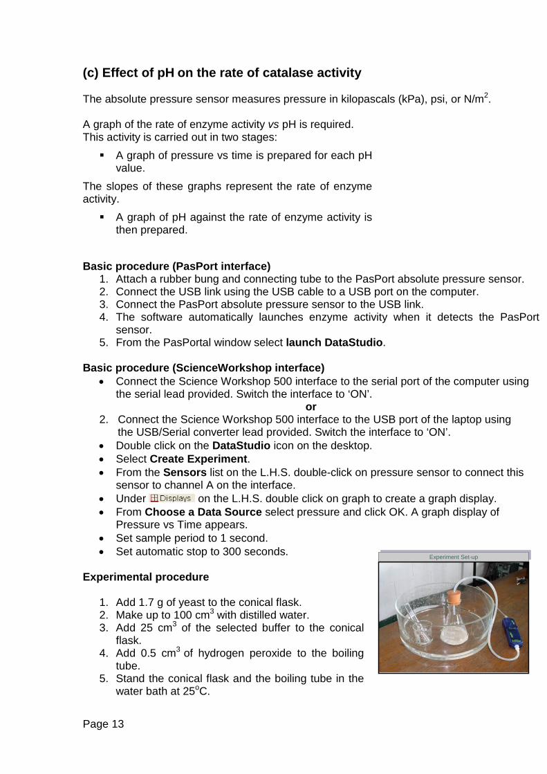
Experimental procedure

1. Add 1.7 g of yeast to the conical flask. 2. Make up to 100 cm3 with distilled water. 3. Add 25 cm3 of the selected buffer to the conical

flask. 4. Add 0.5 cm3 of hydrogen peroxide to the boiling

tube. 5. Stand the conical flask and the boiling tube in the

water bath at 25oC.

Experiment Set-upExperiment Set-up

6. Pour the hydrogen peroxide into the conical flask. 7. Place the rubber bung on the conical flask. 8. On the main toolbar, click the button to start collecting data. 9. Select the Scale to Fit button. 10. The datalogger collects and graphs the data. 11. After the selected time has passed click the Stop button and remove the rubber bung

from the conical flask. A graph labelled Run # 1 has been completed on the screen. 12. Repeat steps 1-11 for each of the selected pH values.

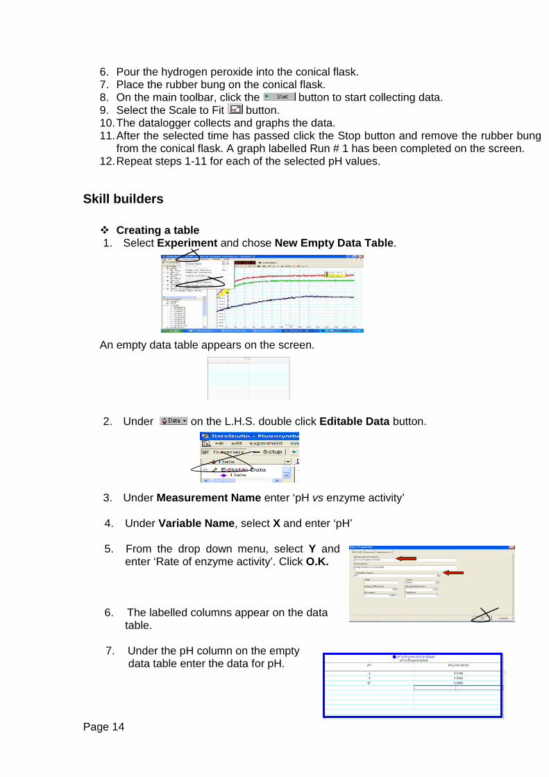
Skill builders Creating a table 1. Select Experiment and chose New Empty Data Table.

An empty data table appears on the screen.

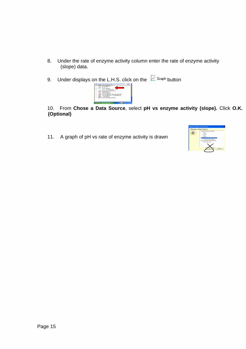
2. Under on the L.H.S. double click Editable Data button.

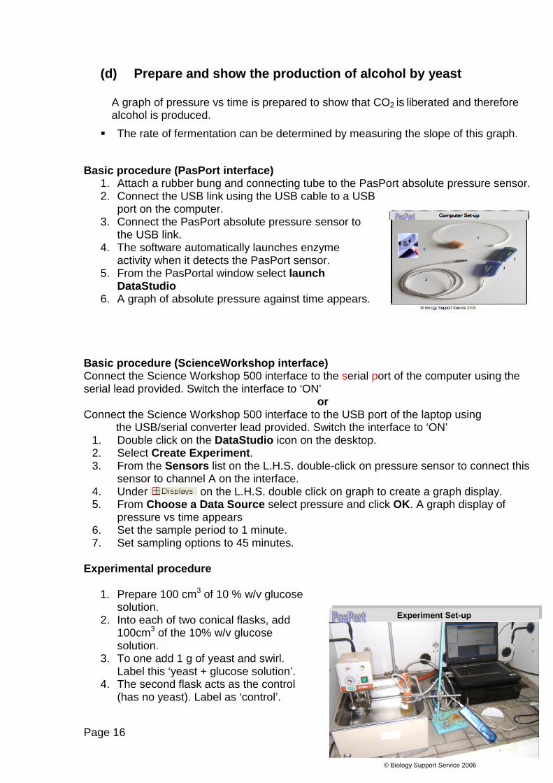
3. Under Measurement Name enter ‘pH vs enzyme activity’ 4. Under Variable Name, select X and enter ‘pH’ 5. From the drop down menu, select Y and

enter ‘Rate of enzyme activity’. Click O.K. 6. The labelled columns appear on the data

table.

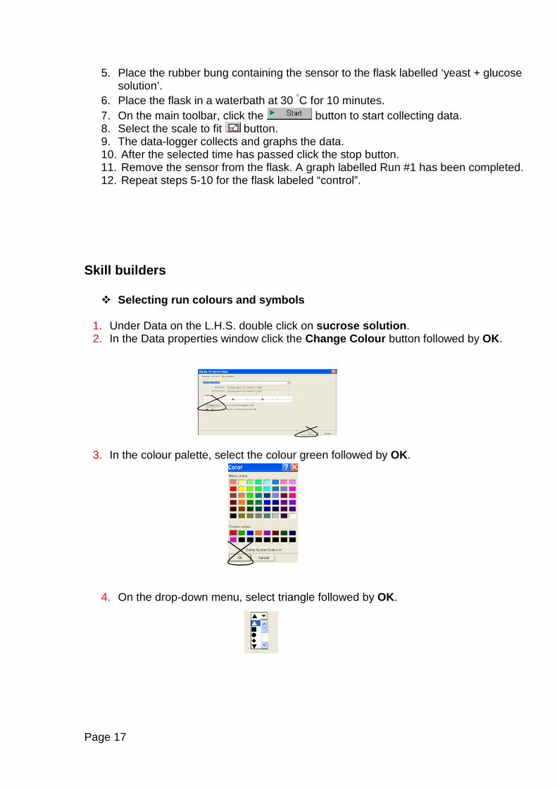
7. Under the pH column on the empty data table enter the data for pH.

8. Under the rate of enzyme activity column enter the rate of enzyme activity

(slope) data. 9. Under displays on the L.H.S. click on the button 10. From Chose a Data Source, select pH vs enzyme activity (slope). Click O.K. (Optional) 11. A graph of pH vs rate of enzyme activity is drawn

(d) Prepare and show the production of alcohol by yeast

A graph of pressure vs time is prepared to show that CO2 is liberated and therefore alcohol is produced.

The rate of fermentation can be determined by measuring the slope of this graph.

Basic procedure (PasPort interface) 1. Attach a rubber bung and connecting tube to the PasPort absolute pressure sensor. 2. Connect the USB link using the USB cable to a USB

port on the computer. 3. Connect the PasPort absolute pressure sensor to

the USB link. 4. The software automatically launches enzyme

activity when it detects the PasPort sensor. 5. From the PasPortal window select launch

DataStudio 6. A graph of absolute pressure against time appears.

Basic procedure (ScienceWorkshop interface) Connect the Science Workshop 500 interface to the serial port of the computer using the serial lead provided. Switch the interface to ‘ON’

or Connect the Science Workshop 500 interface to the USB port of the laptop using

the USB/serial converter lead provided. Switch the interface to ‘ON’ 1. Double click on the DataStudio icon on the desktop. 2. Select Create Experiment. 3. From the Sensors list on the L.H.S. double-click on pressure sensor to connect this

sensor to channel A on the interface. 4. Under on the L.H.S. double click on graph to create a graph display. 5. From Choose a Data Source select pressure and click OK. A graph display of

pressure vs time appears 6. Set the sample period to 1 minute. 7. Set sampling options to 45 minutes.


1. Prepare 100 cm3 of 10 % w/v glucose solution.

2. Into each of two conical flasks, add 100cm3 of the 10% w/v glucose solution.

3. To one add 1 g of yeast and swirl. Label this ‘yeast + glucose solution’.

4. The second flask acts as the control (has no yeast). Label as ‘control’.

© Biology Support Service 2006

Experiment Set-upExperiment Set-up

5. Place the rubber bung containing the sensor to the flask labelled ‘yeast + glucose solution’.

6. Place the flask in a waterbath at 30 ◦C for 10 minutes. 7. On the main toolbar, click the button to start collecting data. 8. Select the scale to fit button. 9. The data-logger collects and graphs the data. 10. After the selected time has passed click the stop button. 11. Remove the sensor from the flask. A graph labelled Run #1 has been completed. 12. Repeat steps 5-10 for the flask labeled “control”.

Skill builders Selecting run colours and symbols

1. Under Data on the L.H.S. double click on sucrose solution. 2. In the Data properties window click the Change Colour button followed by OK.

3. In the colour palette, select the colour green followed by OK.

4. On the drop-down menu, select triangle followed by OK.

Using graph viewing tools Scaling and zooming the graph axes Moving the graph origin

1. Use the zoom in button and zoom out buttons located on the main toolbar and observe their effect.

2. Use the Origin Moving Cursor and observe its effect. 3. Use the X scaling cursor and observe its effect.

4. Use the Y- scaling cursor and observe its effect.

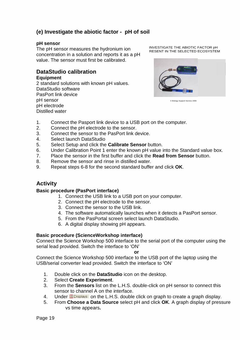
(e) Investigate the abiotic factor - pH of soil

pH sensor The pH sensor measures the hydronium ion concentration in a solution and reports it as a pH value. The sensor must first be calibrated. DataStudio calibration Equipment 2 standard solutions with known pH values. DataStudio software PasPort link device pH sensor pH electrode Distilled water 1. Connect the Pasport link device to a USB port on the computer. 2. Connect the pH electrode to the sensor. 3. Connect the sensor to the PasPort link device. 4. Select launch DataStudio 5. Select Setup and click the Calibrate Sensor button. 6. Under Calibration Point 1 enter the known pH value into the Standard value box. 7. Place the sensor in the first buffer and click the Read from Sensor button. 8. Remove the sensor and rinse in distilled water. 9. Repeat steps 6-8 for the second standard buffer and click OK.

Activity Basic procedure (PasPort interface)

1. Connect the USB link to a USB port on your computer. 2. Connect the pH electrode to the sensor. 3. Connect the sensor to the USB link. 4. The software automatically launches when it detects a PasPort sensor. 5. From the PasPortal screen select launch DataStudio. 6. A digital display showing pH appears.

Basic procedure (ScienceWorkshop interface) Connect the Science Workshop 500 interface to the serial port of the computer using the serial lead provided. Switch the interface to ‘ON’

or Connect the Science Workshop 500 interface to the USB port of the laptop using the USB/serial converter lead provided. Switch the interface to ‘ON’

1. Double click on the DataStudio icon on the desktop. 2. Select Create Experiment. 3. From the Sensors list on the L.H.S. double-click on pH sensor to connect this

sensor to channel A on the interface. 4. Under on the L.H.S. double click on graph to create a graph display. 5. From Choose a Data Source select pH and click OK. A graph display of pressure

vs time appears.

© Biology Support Service 2006

INVESTIGATE THE ABIOTIC FACTOR pH PRESENT IN THE SELECTED ECOSYSTEM

Experimental procedure Measure the pH of a soil sample as follows: Mix the sample with distilled water. Filter the sample. Insert the pH probe into the filtrate. Press the to start collecting data. Press the to stop collecting data. Remove the probe from the sample and rinse with distilled water. Repeat for different samples.

Skill builders

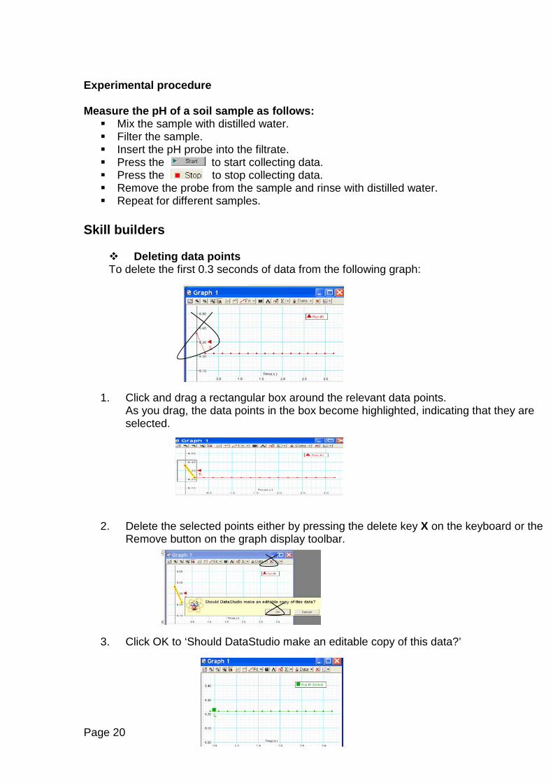
Deleting data points To delete the first 0.3 seconds of data from the following graph:

1. Click and drag a rectangular box around the relevant data points.

As you drag, the data points in the box become highlighted, indicating that they are selected.

2. Delete the selected points either by pressing the delete key X on the keyboard or the Remove button on the graph display toolbar.

3. Click OK to ‘Should DataStudio make an editable copy of this data?’

Under Data the data run is a different colour and is now labeled Run # 1 (Edited). The original Run#3 is still intact.

Using print screen 1. Open pH activity file (if not already open). 2. Press the Print Screen button on the keyboard. 3. Minimise the screen and open a word document. 4. Select paste. The image can then be formatted.

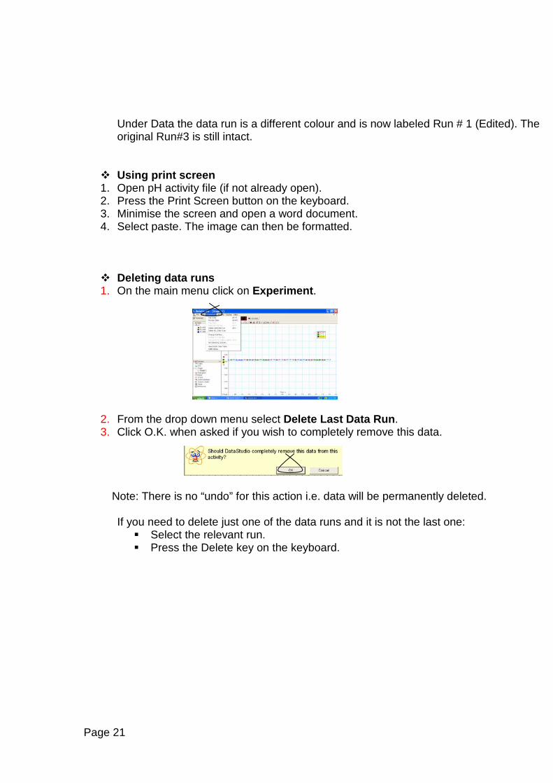
Deleting data runs 1. On the main menu click on Experiment.

2. From the drop down menu select Delete Last Data Run. 3. Click O.K. when asked if you wish to completely remove this data.

Note: There is no “undo” for this action i.e. data will be permanently deleted.

If you need to delete just one of the data runs and it is not the last one: Select the relevant run. Press the Delete key on the keyboard.

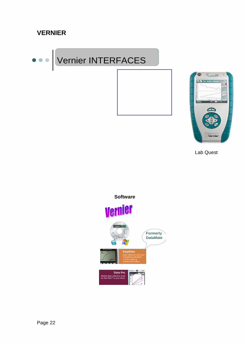
VERNIER

Formerly DataMate

Software

Vernier INTERFACES

Lab Quest

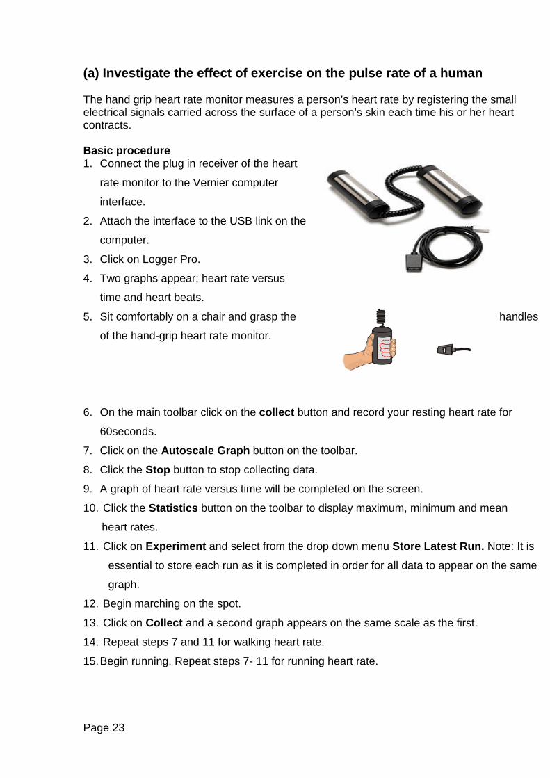
(a) Investigate the effect of exercise on the pulse rate of a human The hand grip heart rate monitor measures a person’s heart rate by registering the small electrical signals carried across the surface of a person’s skin each time his or her heart contracts. Basic procedure 1. Connect the plug in receiver of the heart

rate monitor to the Vernier computer

interface.

2. Attach the interface to the USB link on the

computer.

3. Click on Logger Pro.

4. Two graphs appear; heart rate versus

time and heart beats.

5. Sit comfortably on a chair and grasp the handles

of the hand-grip heart rate monitor.

6. On the main toolbar click on the collect button and record your resting heart rate for

60seconds.

7. Click on the Autoscale Graph button on the toolbar.

8. Click the Stop button to stop collecting data.

9. A graph of heart rate versus time will be completed on the screen.

10. Click the Statistics button on the toolbar to display maximum, minimum and mean

heart rates.

11. Click on Experiment and select from the drop down menu Store Latest Run. Note: It is

essential to store each run as it is completed in order for all data to appear on the same

graph.

12. Begin marching on the spot.

13. Click on Collect and a second graph appears on the same scale as the first.

14. Repeat steps 7 and 11 for walking heart rate.

15. Begin running. Repeat steps 7- 11 for running heart rate.

Results

Condition Rate in beats per minute

Heart rate at rest

Heart rate after marching

Heart rate after running

Skill builders 1. Saving your file From the toolbar go to File and Save Activity As……

Navigate to the folder in which you wish to store your file. Give the file a name followed by

Save.

2. Naming the graph Click on the graph and a graph options box appears. Under title enter heart rate versus time and click on done. The graph is now labelled heart rate versus time.

3. Using the prediction function A prediction can be made on the expected appearance of the graph for each of the selected

exercises. Click on the Analyze button on the toolbar and scroll down to Draw Prediction. A pencil

appears when the cursor is positioned over the graph.

4. Using the annotation function Click on Insert and then on Text Annotation. Enter text e.g. “walking heart rate prediction”.

To remove the Annotation Text Box click on Edit and select Undo. 5. Changing a display Add a table or metre or additional graphs to the screen by clicking on the drop down menu

under the Insert button on the toolbar.

6. Viewing stored data in logger pro

Click on the Open icon on the toolbar (second icon from the left). An experiment file opens.

Click on Sample Data and open. Click on Biology and heart rate to view a completed graph

of the experiment.

Helpful hint Ensure that the arrow on the plug in receiver of the heart rate monitor and the hand grip heart rate monitor are aligned during data collection and that they are no further than 1 metre apart.

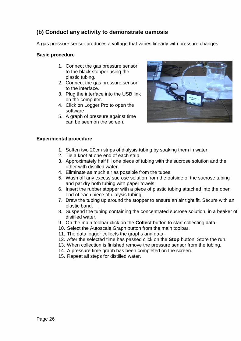
(b) Conduct any activity to demonstrate osmosis A gas pressure sensor produces a voltage that varies linearly with pressure changes. Basic procedure

1. Connect the gas pressure sensor to the black stopper using the plastic tubing.

2. Connect the gas pressure sensor to the interface.

3. Plug the interface into the USB link on the computer.

4. Click on Logger Pro to open the software

5. A graph of pressure against time can be seen on the screen.


1. Soften two 20cm strips of dialysis tubing by soaking them in water. 2. Tie a knot at one end of each strip. 3. Approximately half fill one piece of tubing with the sucrose solution and the

other with distilled water. 4. Eliminate as much air as possible from the tubes. 5. Wash off any excess sucrose solution from the outside of the sucrose tubing

and pat dry both tubing with paper towels. 6. Insert the rubber stopper with a piece of plastic tubing attached into the open

end of each piece of dialysis tubing. 7. Draw the tubing up around the stopper to ensure an air tight fit. Secure with an

elastic band. 8. Suspend the tubing containing the concentrated sucrose solution, in a beaker of

distilled water. 9. On the main toolbar click on the Collect button to start collecting data. 10. Select the Autoscale Graph button from the main toolbar. 11. The data logger collects the graphs and data. 12. After the selected time has passed click on the Stop button. Store the run. 13. When collection is finished remove the pressure sensor from the tubing. 14. A pressure time graph has been completed on the screen. 15. Repeat all steps for distilled water.

1 Sensor

2 LabProinterface

1

2

3

4

5

Skill builders 1. Setting sample periods Click on Experiment on the main toolbar. Then click on Data Collection. Enter 15 minutes into the length box. Set the sample rate to one sample per minute. Then click on done. 2. Finding the slope of the graph Click on the Linear Fit button on the main toolbar. A linear fit for the entire graph is shown. Read and record the value for slope. This figure represents the overall rate of osmosis. The rate between any number of points may be found by highlighting the points of interest and then clicking on Linear Fit. 3. Using the data button When both runs are on the screen they may be viewed separately if necessary. Click on Data on the main toolbar and then on Hide Data Set. Then press latest. One set of data is removed. It may be replaced by clicking on Data Set Options and then on Latest. Remove the tick from hide data set and click on ok.

(c) Investigate the effect of pH on the rate of catalase activity This activity is carried out in two stages

• A graph of pressure vs time is prepared for each pH value. The slopes of these graphs represent the rate of enzyme activity.

• A graph of pH against the rate of enzyme activity is then prepared Basic procedure

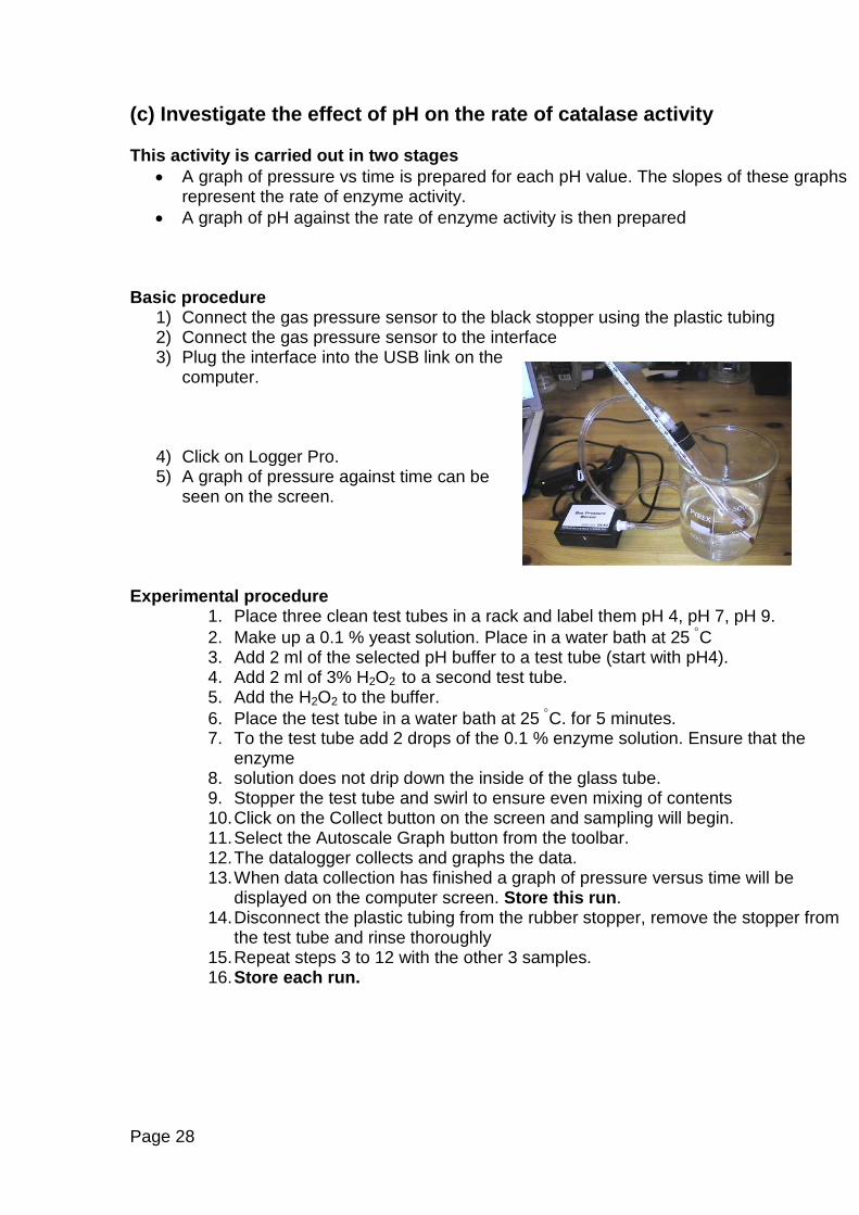
1) Connect the gas pressure sensor to the black stopper using the plastic tubing 2) Connect the gas pressure sensor to the interface 3) Plug the interface into the USB link on the

computer.

4) Click on Logger Pro. 5) A graph of pressure against time can be

seen on the screen. Experimental procedure

1. Place three clean test tubes in a rack and label them pH 4, pH 7, pH 9. 2. Make up a 0.1 % yeast solution. Place in a water bath at 25 °C 3. Add 2 ml of the selected pH buffer to a test tube (start with pH4). 4. Add 2 ml of 3% H2O2 to a second test tube. 5. Add the H2O2 to the buffer. 6. Place the test tube in a water bath at 25 °C. for 5 minutes. 7. To the test tube add 2 drops of the 0.1 % enzyme solution. Ensure that the

enzyme 8. solution does not drip down the inside of the glass tube. 9. Stopper the test tube and swirl to ensure even mixing of contents 10. Click on the Collect button on the screen and sampling will begin. 11. Select the Autoscale Graph button from the toolbar. 12. The datalogger collects and graphs the data. 13. When data collection has finished a graph of pressure versus time will be

displayed on the computer screen. Store this run. 14. Disconnect the plastic tubing from the rubber stopper, remove the stopper from

the test tube and rinse thoroughly 15. Repeat steps 3 to 12 with the other 3 samples. 16. Store each run.

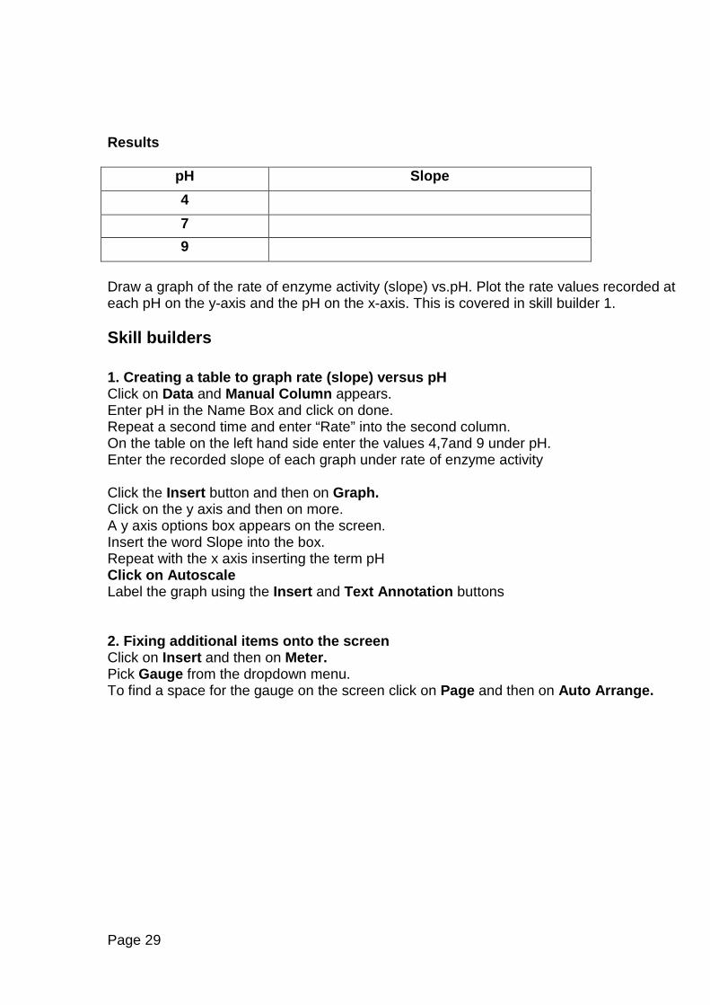
Results

pH Slope 4 7 9

Draw a graph of the rate of enzyme activity (slope) vs.pH. Plot the rate values recorded at each pH on the y-axis and the pH on the x-axis. This is covered in skill builder 1. Skill builders 1. Creating a table to graph rate (slope) versus pH Click on Data and Manual Column appears. Enter pH in the Name Box and click on done. Repeat a second time and enter “Rate” into the second column. On the table on the left hand side enter the values 4,7and 9 under pH. Enter the recorded slope of each graph under rate of enzyme activity Click the Insert button and then on Graph. Click on the y axis and then on more. A y axis options box appears on the screen. Insert the word Slope into the box. Repeat with the x axis inserting the term pH Click on Autoscale Label the graph using the Insert and Text Annotation buttons 2. Fixing additional items onto the screen Click on Insert and then on Meter. Pick Gauge from the dropdown menu. To find a space for the gauge on the screen click on Page and then on Auto Arrange.

(d) Prepare and show the production of Alcohol by Yeast A gas pressure produces a voltage, which varies linearly with pressure changes. • Prepare a pressure versus time graph to show that CO2 is liberated and therefore alcohol

is produced. • The rate of fermentation can be determined by measuring the slope of the graph. Basic Procedure 1. Connect the gas pressure sensor to the black stopper using the plastic tubing 2. Connect the gas pressure sensor to the interface 3. Plug the interface into the USB link on the computer 4. Click on logger pro to open the software 5. A graph of pressure against time can be seen on the screen 6. Set sample period to 45 minutes 7. Set sampling rate to 1 per minute

Experimental procedure 1. Set up a water bath at 300C. 2. Prepare 100cm3 or a 10% w/v glucose solution. 3. Half fill two test tubes with glucose solution. 4. To one, add 0. 5g of yeast and swirl. Label this yeast + glucose solution. 5. The second flask acts as a control (has no yeast) label as control. 6. Insert a one holed rubber stopper assembly into the flask labelled yeast and glucose

solution. 7. Place the test tube in the water bath for 10 minutes. 8. Click on Collect on the computer to start data collection. 9. Select the Autoscale graph button. 10. The data logger collects and graphs the data. 11. Data collection will end after 45 minutes. 12. When the data is collected a graph of pressure versus time will be on the computer

screen Skill builders 1. Selecting Run Colours and Symbols Double click on the graph and the Graph Options Menu opens. Click on the down arrow opposite the title box and change the colour of the graph title to violet. Staying in the same menu move to the Grid Box click on the top box with Grey and from the drop down menu select Custom. The Colour Palette appears, select the colour Green followed by ok. Click on the down arrow in the grid box and under major tick style select Dotted from the menu to change the graph style.

In the appearance menu click on Bar Graph “followed by “done”. The line graph changes to a bar graph. To undo this deselect the ticked box 2. Using Graph Viewing Tools Scaling and zooming the graph axes. Use the zoom in buttons and zoom out buttons located on the main toolbar and observe their effect 3. Moving the Graph Origin Click on the left and right arrows beside time on the x axis to move the origin. Click on the left and right arrows beside Pressure on the y axis to move the graph up or down 4. Recording values at given times Click on the Examine button on the main toolbar and move the cursor to the graph note how pressure time values are displayed.

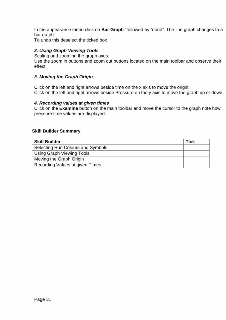
Skill Builder Summary Skill Builder Tick Selecting Run Colours and Symbols Using Graph Viewing Tools Moving the Graph Origin Recording Values at given Times

(e) Investigate the abiotic Factor – pH - in the selected ecosystem Important: Do not let the pH electrode dry out. Keep it in a 250 ml beaker with about 100 ml of tap water when not in use. The tip of the probe is made of glass—it is fragile. Handle with care! Basic procedure Connect the interface to the USB link on the computer. Connect the pH sensor to the interface. Start logger pro. A digital display showing pH appears. Set the sample rate to 5 samples per second. Experimental procedure - measure the pH of a soil sample as follows 1. Mix the sample with distilled water. 2. Filter the sample. 3. Insert the pH probe into the filtrate. 4. Press the Collect button to start collecting data. 5. Press the Stop button to stop collecting data. 6. Remove the probe from the sample and rinse with distilled water. 7. Repeat for different samples. Skill builders 1. Deleting Data Points Click on the table where the data is being recorded. It is now highlighted. Now click on the value you wish to remove. Click on Edit and then on Strike Through Data Cells A line appears through the point in the Table and the point is removed from the graph. 2. Using the Print Screen Key When a graph is finished press the Print Screen on they keyboard. Minimize the screen and open a Word Document. Click on Paste and the completed graph is copied into a word file. Name it and save it. 3. Deleting a Data Set When two or more graphs are present on the screen one may be removed.

Click on Data and then on Delete Data Set. You are then given the option of which run to delete. Click on the one you wish to remove. Click on Edit and Undo Delete Data Set to restore the graph. Skill Builders Summary Skill Builders Tick

Deleting Data Points

Using Print Screen

Deleting a Data Set

Calibration of sensor Sensors normally do not require calibration as the chip in the handle stores the calibration values. If you wish to calibrate a sensor the instructions are below. Equipment 2 standard solutions with known pH values Logger pro software Interface link pH sensor Distilled water Logger Pro two point calibration 1. Connect the interface to the USB link on the computer. 2. Attach the pH sensor to the interface. 3. Start logger pro. 4. Remove the storage bottle from the electrode by first unscrewing the lid, then removing

the bottle and lid. 5. Rinse the lower section containing the bulb with distilled water. 6. Click on Experiment on the toolbar. 7. Click on Calibrate. 8. From the Sensor Setting Menu. 9. Click on Calibrate Now. Click on the interface and sensor opposite calibrate. 10. Put the sensor into pH 7 solution. A pH value is registered on the screen. When the value

stabilises enter 7 into the first reading box and click on keep. 11. Rinse with distilled water 12. Put the sensor into a pH 4 buffer solution. A new pH value is recorded. When the value

stabilises, enter 4 into the second reading box and click on keep. 13. Rinse sensor with distilled water and return it to the original storage bottle. (Remember to

slide the cap onto the electrode body and then twist it onto the storage bottle). 14. Disconnect the sensor from the interface.

datalogging - pdst · datalogging allows real-time data such as ... advisable to connect your...

Documents