Data Warehousing & OLAPData Warehousing & OLAP

2

What is Data Warehouse?

• “A data warehouse is a subject-oriented, integrated, time-variant, and nonvolatile collection of data in support of management’s decision-making process.”—W. H. Inmon

• A Data Warehouse is used for On-Line-Analytical-Processing:“Class of tools that enables the user to gain insight into data through

interactive access to a wide variety of possible views of the information”

• 3 Billion market worldwide [1999 figure, olapreport.com]

– Retail industries: user profiling, inventory management– Financial services: credit card analysis, fraud detection– Telecommunications: call analysis, fraud detection

3

Data Warehouse Initiatives

• Organized around major subjects, such as customer, product, sales – integrate multiple, heterogeneous data sources

– exclude data that are not useful in the decision support process

• Focusing on the modeling and analysis of data for decision makers, not on daily operations or transaction processing– emphasis is on complex, exploratory analysis not day-to-day

operations

• Large time horizon for trend analysis (current and past data)

• Non-Volatile store– physically separate store from the operational environment

4

Data Warehouse Architecture

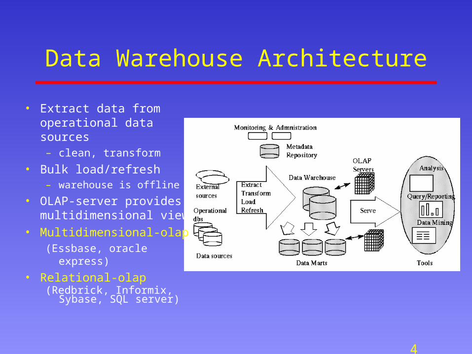
• Extract data from operational data sources– clean, transform

• Bulk load/refresh– warehouse is offline

• OLAP-server provides multidimensional view

• Multidimensional-olap (Essbase, oracle express)

• Relational-olap(Redbrick, Informix, Sybase,

SQL server)

5

Why do we need all that?

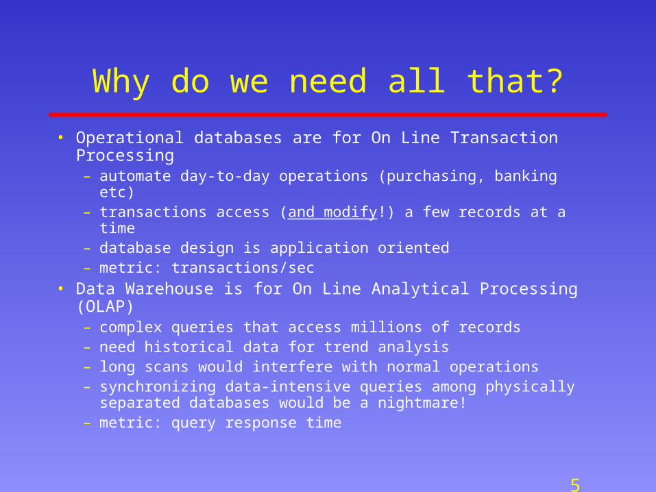
• Operational databases are for On Line Transaction Processing– automate day-to-day operations (purchasing, banking etc)– transactions access (and modify!) a few records at a time– database design is application oriented– metric: transactions/sec

• Data Warehouse is for On Line Analytical Processing (OLAP)– complex queries that access millions of records– need historical data for trend analysis – long scans would interfere with normal operations– synchronizing data-intensive queries among physically separated

databases would be a nightmare!– metric: query response time

6

Examples of OLAP

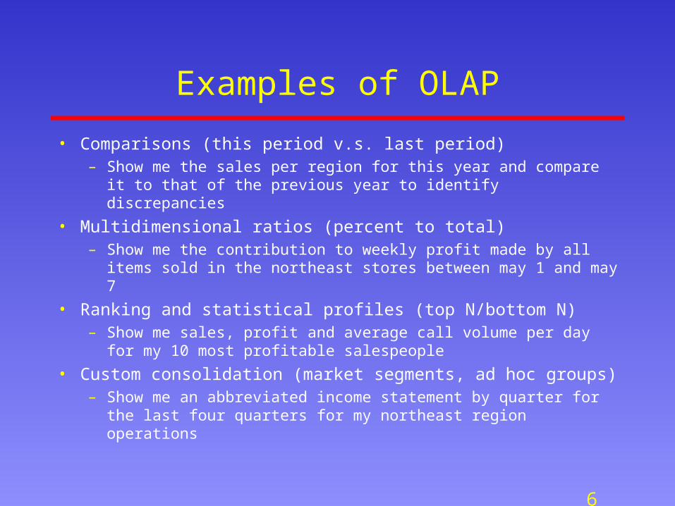
• Comparisons (this period v.s. last period)– Show me the sales per region for this year and compare it to that of

the previous year to identify discrepancies

• Multidimensional ratios (percent to total)– Show me the contribution to weekly profit made by all items sold in

the northeast stores between may 1 and may 7

• Ranking and statistical profiles (top N/bottom N)– Show me sales, profit and average call volume per day for my 10

most profitable salespeople

• Custom consolidation (market segments, ad hoc groups)– Show me an abbreviated income statement by quarter for the last

four quarters for my northeast region operations

7

Multidimensional Modeling

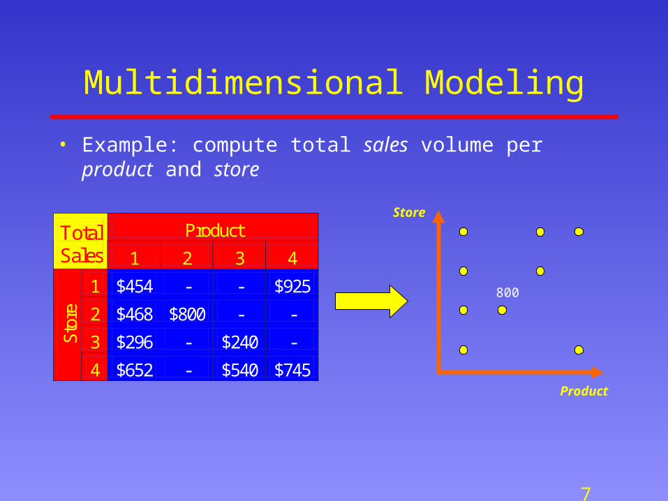
• Example: compute total sales volume per product and store

Product Total Sales 1 2 3 4

1 $454 - - $925

2 $468 $800 - -

3 $296 - $240 - Sto

re

4 $652 - $540 $745

Product

Store

800

8

Dimensions and Hierarchiespr

oduc

tcit

y

month

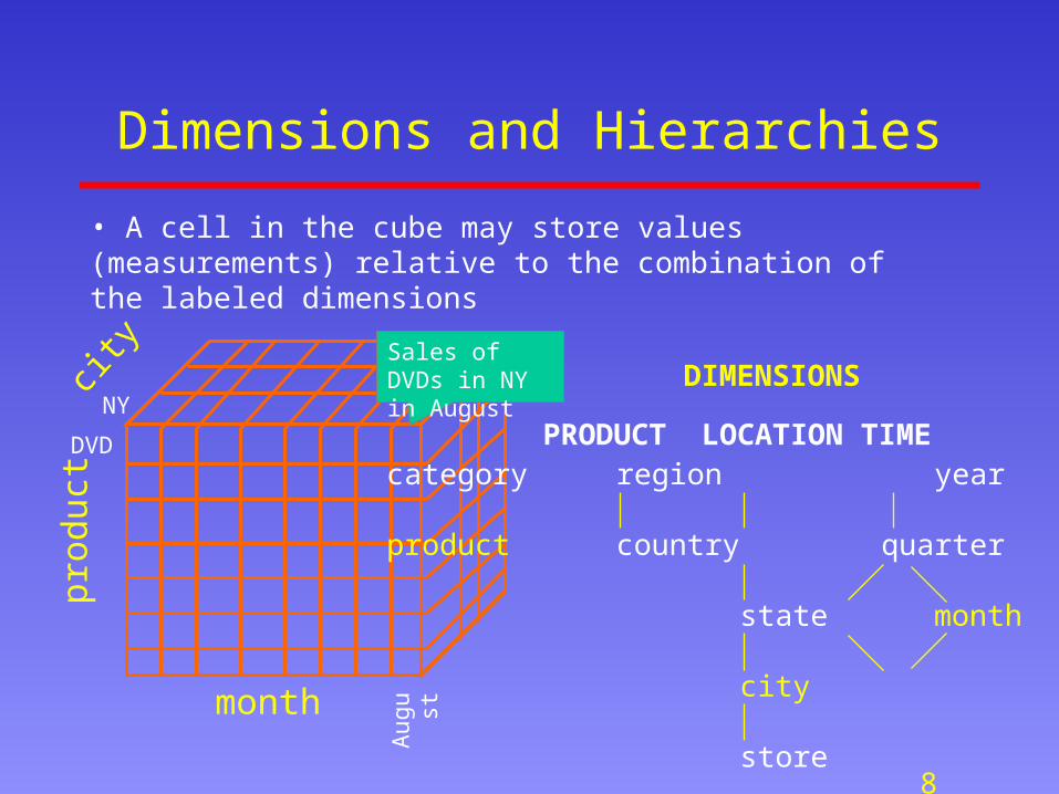
category region year

product country quarter

state month week

city day

store

PRODUCT LOCATION TIMENY

DVD

Aug

ust

Sales of DVDs in NY in August

• A cell in the cube may store values (measurements) relative to the combination of the labeled dimensions

DIMENSIONS

9

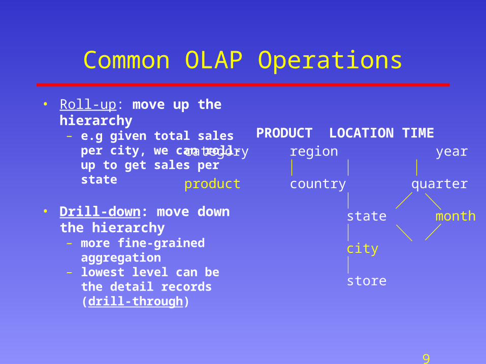
Common OLAP Operations

• Roll-up: move up the hierarchy– e.g given total sales per city, we

can roll-up to get sales per state

• Drill-down: move down the hierarchy– more fine-grained aggregation– lowest level can be the detail

records (drill-through)

category region year

product country quarter

state month week

city day

store

PRODUCT LOCATION TIME

10

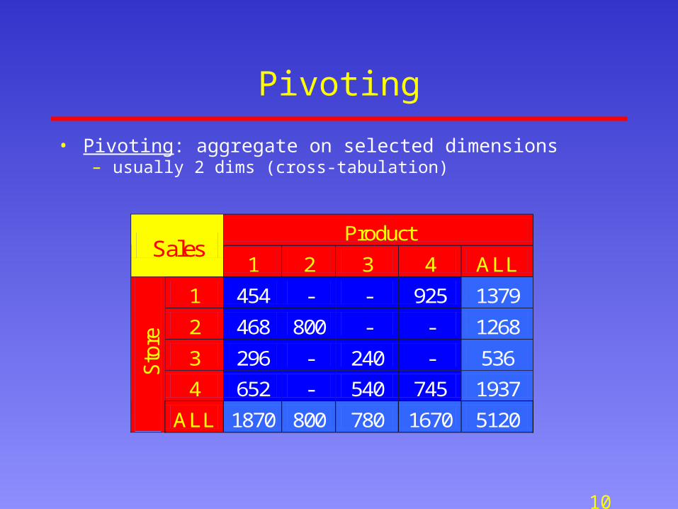
Pivoting

• Pivoting: aggregate on selected dimensions– usually 2 dims (cross-tabulation)

Product Sales

1 2 3 4 ALL

1 454 - - 925 1379

2 468 800 - - 1268

3 296 - 240 - 536

4 652 - 540 745 1937

Sto

re

ALL 1870 800 780 1670 5120

11

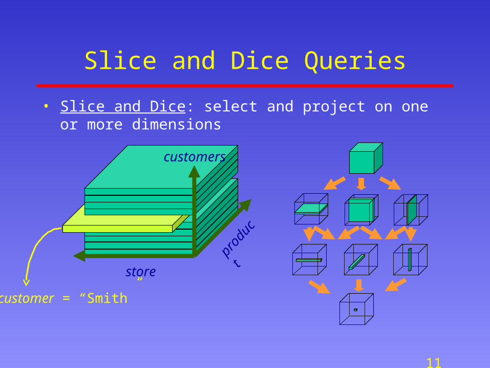
Slice and Dice Queries

• Slice and Dice: select and project on one or more dimensions

prod

uct

customers

store

customer = “Smith”

12

Roadmap

• What is a data warehouse and what it is for

• What are the differences between OLTP and OLAP

• Multi-dimensional data modeling

• Data warehouse design– the star schema, bitmap indexes

• The Data Cube operator– semantics and computation

• Aggregate View Selection

• Other Issues

13

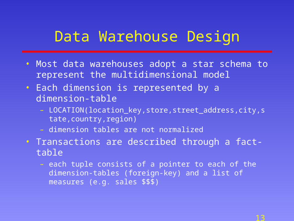
Data Warehouse Design

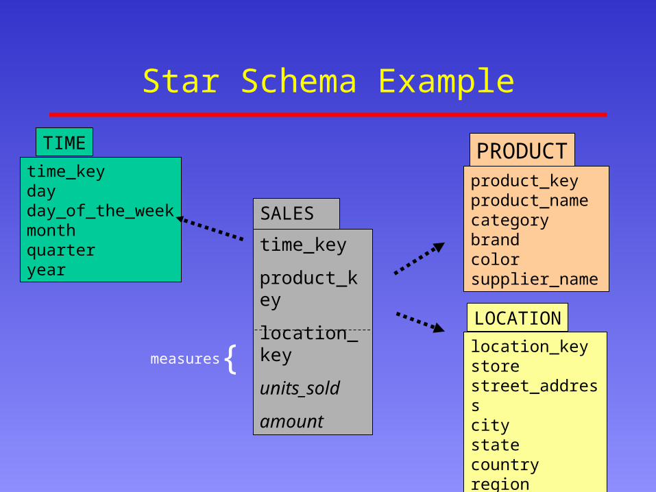
• Most data warehouses adopt a star schema to represent the multidimensional model

• Each dimension is represented by a dimension-table– LOCATION(location_key,store,street_address,city,state,country,region)

– dimension tables are not normalized

• Transactions are described through a fact-table– each tuple consists of a pointer to each of the dimension-tables (foreign-

key) and a list of measures (e.g. sales $$$)

14

Star Schema Example

time_keydayday_of_the_weekmonthquarteryear

TIME

location_keystorestreet_addresscitystatecountryregion

LOCATION

SALES

product_keyproduct_namecategorybrandcolorsupplier_name

PRODUCT

time_key

product_key

location_key

units_sold

amount{measures

15

Advantages of Star Schema

• Facts and dimensions are clearly depicted– dimension tables are relatively static, data is loaded (append

mostly) into fact table(s)

– easy to comprehend (and write queries)

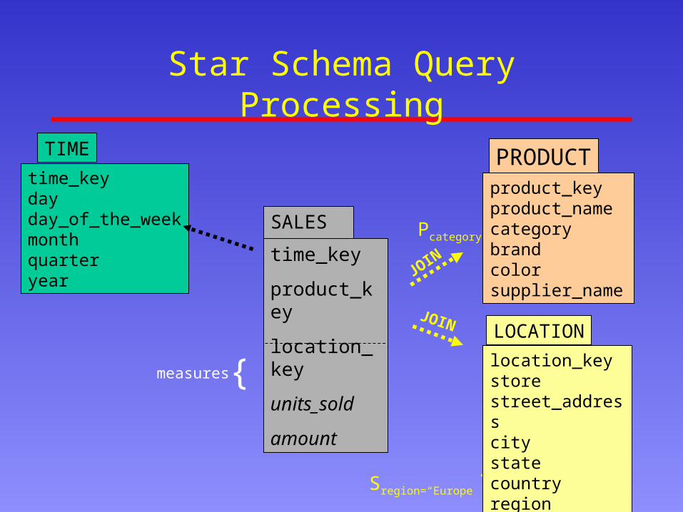
“Find total sales per product-category in our stores in Europe”

SELECT PRODUCT.category, SUM(SALES.amount)

FROM SALES, PRODUCT,LOCATION

WHERE SALES.product_key = PRODUCT.product_key

AND SALES.location_key = LOCATION.location_key

AND LOCATION.region=“Europe”

GROUP BY PRODUCT.category

16

Star Schema Query Processing

time_keydayday_of_the_weekmonthquarteryear

TIME

location_keystorestreet_addresscity statecountryregion

LOCATION

SALES

product_keyproduct_namecategorybrandcolorsupplier_name

PRODUCT

time_key

product_key

location_key

units_sold

amount{measures

JOIN

JOIN

Sregion=“Europe”

Pcategory

17

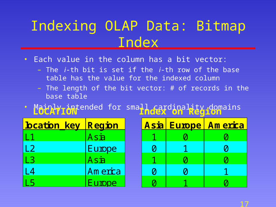
Indexing OLAP Data: Bitmap Index

• Each value in the column has a bit vector: – The i-th bit is set if the i-th row of the base table has the value for the

indexed column

– The length of the bit vector: # of records in the base table

• Mainly intended for small cardinality domains

location_key RegionL1 AsiaL2 EuropeL3 AsiaL4 AmericaL5 Europe

Asia Europe America1 0 00 1 01 0 00 0 10 1 0

LOCATION Index on Region

18

R102

R117

R118

R124

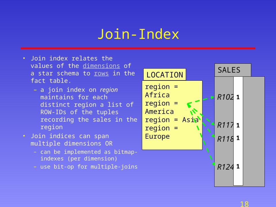
Join-Index

• Join index relates the values of the dimensions of a star schema to rows in the fact table.

– a join index on region maintains for each distinct region a list of ROW-IDs of the tuples recording the sales in the region

• Join indices can span multiple dimensions OR– can be implemented as bitmap-

indexes (per dimension)

– use bit-op for multiple-joins

SALES

region = Africaregion = Americaregion = Asiaregion = Europe

LOCATION

1

1

1

1

19

Problem Solved?

• “Find total sales per product-category in our stores in Europe”

– Join-index will prune ¾ of the data (uniform sales), but the remaining ¼ is still large (several millions transactions)

• Index is unclustered

• High level aggregations are expensive!!!!!– long scans to get the data

– hashing or sorting necessary for group-bys

region

country

state

city

store

LOCATON

Long Query Response Times

Pre-computation is necessary

20

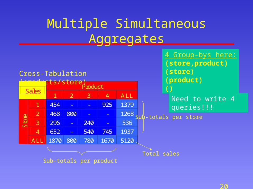
Multiple Simultaneous Aggregates

Product Sales

1 2 3 4 ALL

1 454 - - 925 1379

2 468 800 - - 1268

3 296 - 240 - 536

4 652 - 540 745 1937

Sto

re

ALL 1870 800 780 1670 5120

Cross-Tabulation (products/store)

Sub-totals per store

Sub-totals per productTotal sales

4 Group-bys here:(store,product)(store)(product)()

Need to write 4 queries!!!

21

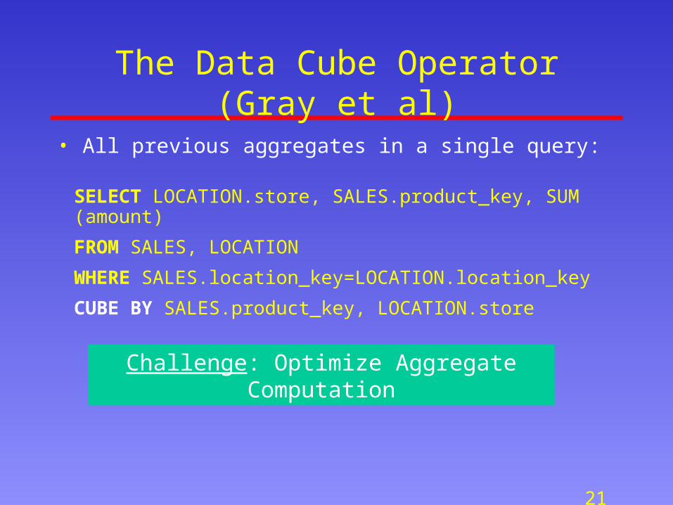
The Data Cube Operator (Gray et al)

• All previous aggregates in a single query:

SELECT LOCATION.store, SALES.product_key, SUM (amount)

FROM SALES, LOCATION

WHERE SALES.location_key=LOCATION.location_key

CUBE BY SALES.product_key, LOCATION.store

Challenge: Optimize Aggregate Computation

22

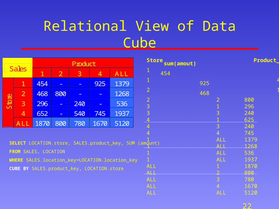
Store Product_key sum(amout)1 1 4541 4 9252 1 4682 2 8003 1 2963 3 2404 1 6254 3 2404 4 7451 ALL 13791 ALL 12681 ALL 5361 ALL 1937ALL 1 1870ALL 2 800ALL 3 780ALL 4 1670ALL ALL 5120

Relational View of Data Cube

Product Sales

1 2 3 4 ALL

1 454 - - 925 1379

2 468 800 - - 1268

3 296 - 240 - 536

4 652 - 540 745 1937

Sto

re

ALL 1870 800 780 1670 5120

SELECT LOCATION.store, SALES.product_key, SUM (amount)

FROM SALES, LOCATION

WHERE SALES.location_key=LOCATION.location_key

CUBE BY SALES.product_key, LOCATION.store

23

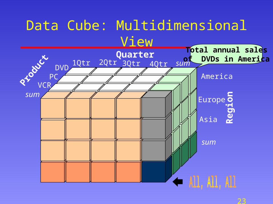
Data Cube: Multidimensional ViewTotal annual sales

of DVDs in AmericaQuarter

Produ

ct

Reg

ionsum

sum DVD

VCRPC

1Qtr 2Qtr 3Qtr 4Qtr

America

Europe

Asia

sum

24

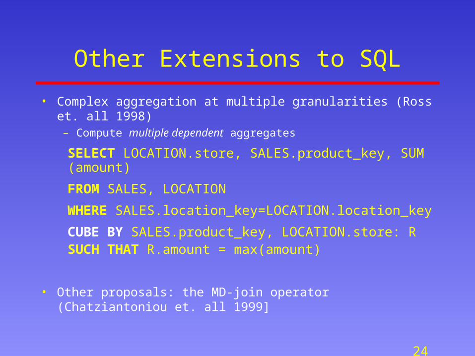
Other Extensions to SQL

• Complex aggregation at multiple granularities (Ross et. all 1998)– Compute multiple dependent aggregates

• Other proposals: the MD-join operator (Chatziantoniou et. all 1999]

SELECT LOCATION.store, SALES.product_key, SUM (amount)

FROM SALES, LOCATION

WHERE SALES.location_key=LOCATION.location_key

CUBE BY SALES.product_key, LOCATION.store: RSUCH THAT R.amount = max(amount)

25

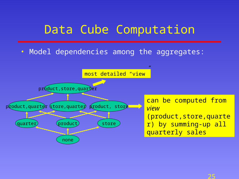
Data Cube Computation

• Model dependencies among the aggregates:

most detailed “view”

can be computed from view (product,store,quarter) by summing-up all quarterly sales

product,store,quarter

product storequarter

none

store,quarterproduct,quarter product, store

26

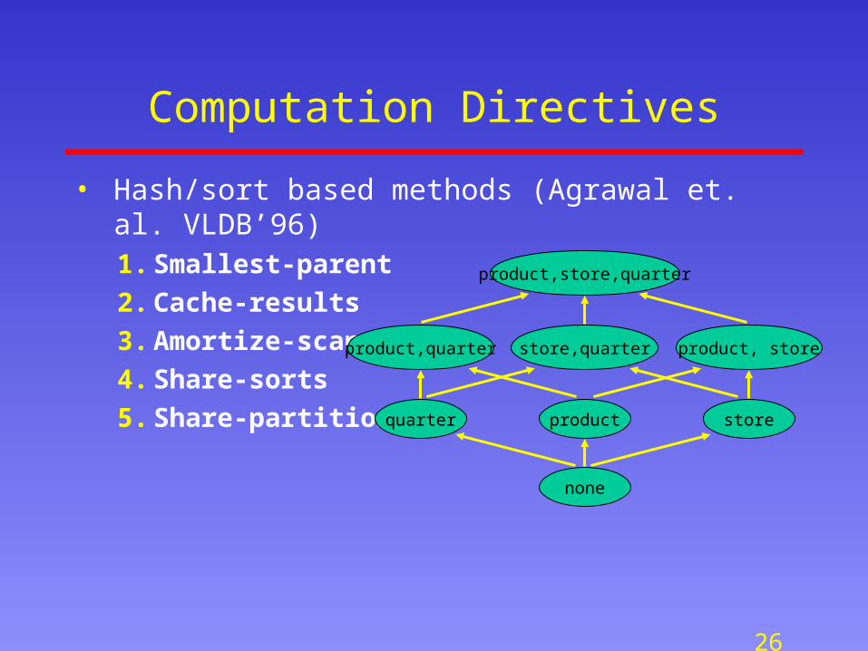
Computation Directives

• Hash/sort based methods (Agrawal et. al. VLDB’96)1. Smallest-parent

2. Cache-results

3. Amortize-scans

4. Share-sorts

5. Share-partitions

product,store,quarter

product storequarter

none

store,quarterproduct,quarter product, store

27

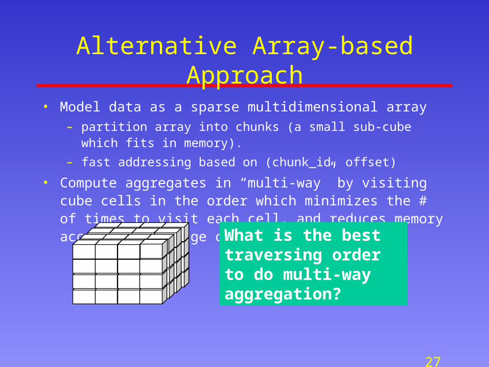
Alternative Array-based Approach

• Model data as a sparse multidimensional array– partition array into chunks (a small sub-cube which fits in memory).

– fast addressing based on (chunk_id, offset)

• Compute aggregates in “multi-way” by visiting cube cells in the order which minimizes the # of times to visit each cell, and reduces memory access and storage cost.

BWhat is the best traversing order to do multi-way aggregation?

28

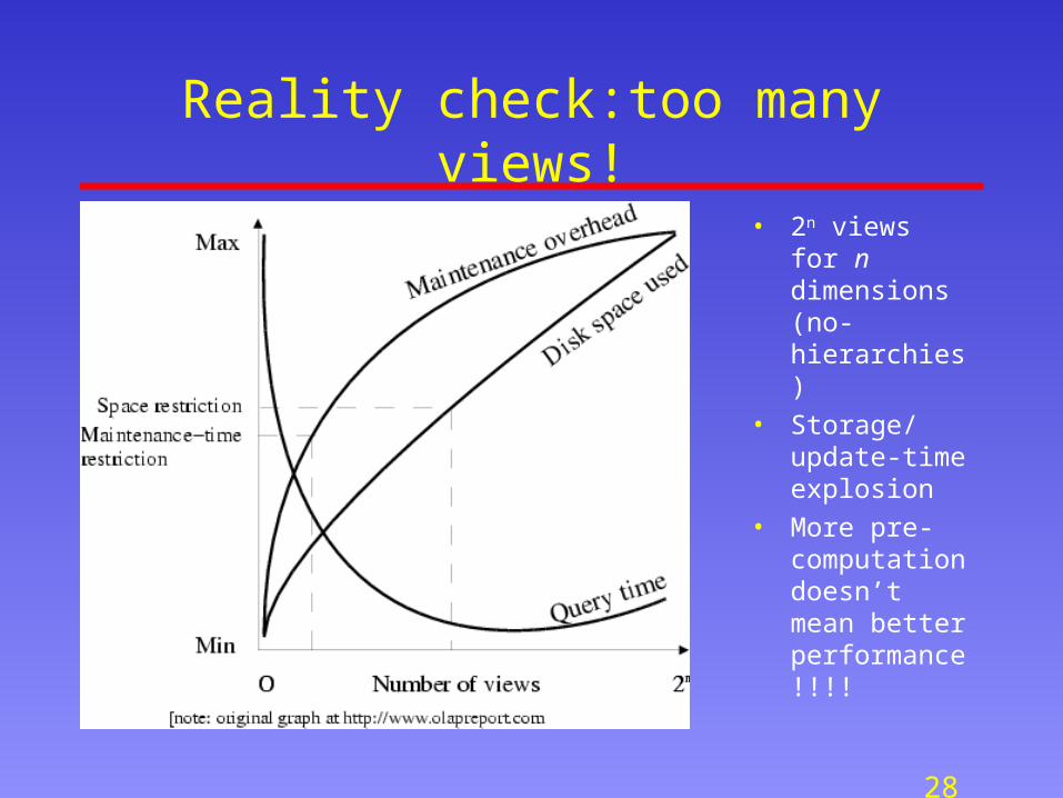
Reality check:too many views!

• 2n views for n dimensions (no-hierarchies)

• Storage/update-time explosion

• More pre-computation doesn’t mean better performance!!!!

29

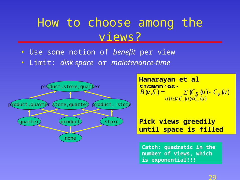
How to choose among the views?

• Use some notion of benefit per view

• Limit: disk space or maintenance-time

product,store,quarter

product storequarter

none

store,quarterproduct,quarter product, store

Hanarayan et al SIGMOD’96:

Pick views greedily until space is filled

)()(,:

))()((),(uCuCvuu

vSSv

uCuCSvB

Catch: quadratic in the number of views, which is exponential!!!

30

View Selection Problem

• Selection is based on a workload estimate (e.g. logs) and a given constraint (disk space or update window)

• NP-hard, optimal selection can not be computed > 4-5 dimensions– greedy algorithms (e.g. [Harinarayan96]) run at least in polynomial time in

the number of views i.e exponential in the number of dimensions!!!• Optimal selection can not be approximated [Karloff99]

– greedy view selection can behave arbitrary bad

• Lack of good models for a cost-based optimization!

31

Other Issues

• Fact+Dimension tables in the DW are views of tables stored in the sources

• Lots of view maintenance problems– correctly reflect asynchronous changes at the sources

– making views self-maintainable

• Interactive queries (on-line aggregation)– e.g. show running-estimates + confidence intervals

• Computing Iceberg queries efficiently

• Approximation– rough-estimates for hi-level aggregates are often good-enough

– histogram, wavelet, sampling based techniques (e.g. AQUA)