Naeem A. Mahoto

Department of Software Engineering Mehran Univeristy of Engineering and Technology Jamshoro

Email: naeemmahoto@gmail.com

Data warehouse and Data Mining Lecture No. 13

Teradata Architecture and its compoenets

Teradata •  Teradata is a relational database management

system (RDBMS): –  Designed to run the world’s largest commercial

databases –  Preferred solution for enterprise data warehousing –  Runs on single or multiple nodes –  Acts as a database server to client applications

throughout the enterprise –  Uses parallelism to manage terabytes of data –  Open, UNIX-based or NT-based system platforms

Teradata - A brief History

Teradata DATABASE

Win 95 Win NT

IBM Main- frame

UNIX

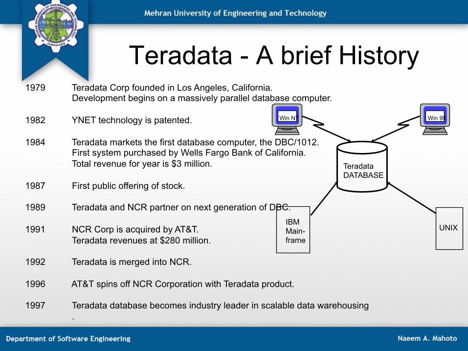
1979 Teradata Corp founded in Los Angeles, California. Development begins on a massively parallel database computer.

1982 YNET technology is patented. 1984 Teradata markets the first database computer, the DBC/1012.

First system purchased by Wells Fargo Bank of California. Total revenue for year is $3 million.

1987 First public offering of stock. 1989 Teradata and NCR partner on next generation of DBC. 1991 NCR Corp is acquired by AT&T.

Teradata revenues at $280 million. 1992 Teradata is merged into NCR. 1996 AT&T spins off NCR Corporation with Teradata product. 1997 Teradata database becomes industry leader in scalable data warehousing

.

The Teradata Charter •  Relational database •  Enormous capacity

–  Billions of rows –  Terabytes of data

•  High-performance parallel processing •  Single database server for multiple clients •  Industry standard access language (SQL) •  Manageable growth via modularity •  Fault tolerance at all levels of hardware and software •  Data integrity and reliability

1 Kilobyte = 103 bytes 1 Megabyte = 106 bytes 1 Gigabyte = 109 bytes 1 Terabyte = 1012 bytes 1 Petabyte = 1015 bytes 1 Exabyte = 1018 bytes 1 Zetabyte = 1021 bytes 1 Yottabyte = 1024 bytes

Components of Teradata System

AMP AMP AMP AMP

Parsing Engine(s) (PEs)

BYNET

Disk Storage

Disk Storage

Disk Storage

Disk Storage

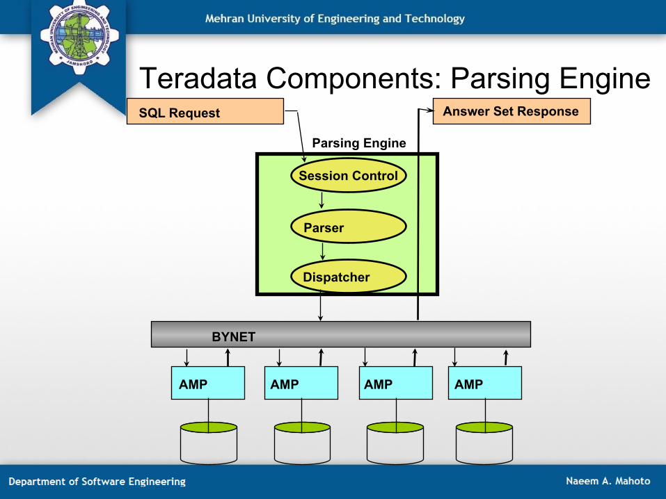
Teradata Components: Parsing Engine

BYNET

AMP AMP AMP AMP

SQL Request Answer Set Response

Parsing Engine

Session Control

Parser

Dispatcher

Teradata Components: Parsing Engine

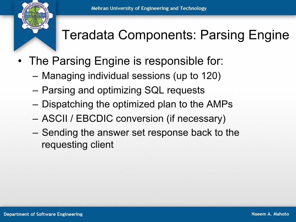
•  The Parsing Engine is responsible for: –  Managing individual sessions (up to 120) –  Parsing and optimizing SQL requests –  Dispatching the optimized plan to the AMPs –  ASCII / EBCDIC conversion (if necessary) –  Sending the answer set response back to the

requesting client

Teradata Components: BYNET •  The BYNET is responsible for:

–  Carrying messages between the AMPs and PEs. –  Broadcasting, point-to-point, or point-to-multipoint

communications. –  Merging answer sets back to the PE. –  Making Teradata parallelism possible.

•  The BYNET is implemented for multi-node or single-node systems

The Access Module Processor (AMP)

•  AMPs are responsible for: –  Finding requested rows –  Lock management –  Sorting rows –  Aggregating columns –  Join processing –  Output conversion and formatting –  Creating answer sets for clients –  Disk space management –  Accounting –  Special utility protocols –  Recovery processing

AMPs store and retrieve rows to and from the disks. An AMP can control up to 64 physical disks.

Disk storage – Disk Arrays AMP 1

vproc

AMP 2

vproc

AMP 3

vproc

AMP 4

vproc

Rank1 Rank2 Rank3 Rank4

•  Each AMP vproc is assigned to a vdisk.

•  A vdisk may contain 119 GB of disk space.

Disk Array Raid Protection •  Two kinds of protection are currently available

with Teradata disk arrays.

•  RAID-1 (Mirroring) –  Each physical disk in the array has an exact copy in the same

array. –  The array controller can read from either disk and write to both. –  When one disk of the pair fails, there is no change in

performance. –  Mirroring reduces available disk space by 50%. –  Array controller reconstructs failed disks quickly.

Primary Mirror

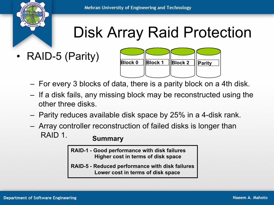
Disk Array Raid Protection •  RAID-5 (Parity)

–  For every 3 blocks of data, there is a parity block on a 4th disk. –  If a disk fails, any missing block may be reconstructed using the

other three disks. –  Parity reduces available disk space by 25% in a 4-disk rank. –  Array controller reconstruction of failed disks is longer than

RAID 1.

Parity Block 0 Block 2 Block 1

Summary RAID-1 - Good performance with disk failures Higher cost in terms of disk space

RAID-5 - Reduced performance with disk failures Lower cost in terms of disk space

Teradata Storage Process •  The Parsing Engine

dispatches a request to insert a row.

•  The BYNET ensures that the row gets to the appropriate AMP (Access Module Processor).

•  The AMP stores the row on its associated disk.

•  Each AMP can have multiple physical disks associated with it.

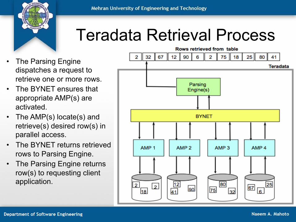
Teradata Retrieval Process •  The Parsing Engine

dispatches a request to retrieve one or more rows.

•  The BYNET ensures that appropriate AMP(s) are activated.

•  The AMP(s) locate(s) and retrieve(s) desired row(s) in parallel access.

•  The BYNET returns retrieved rows to Parsing Engine.

•  The Parsing Engine returns row(s) to requesting client application.

Multiple Tables on Multiple AMPs

•  Some rows from each table may be found on each AMP.

•  Each AMP may have rows from all tables.

•  Ideally, each AMP will hold roughly the same amount of data.

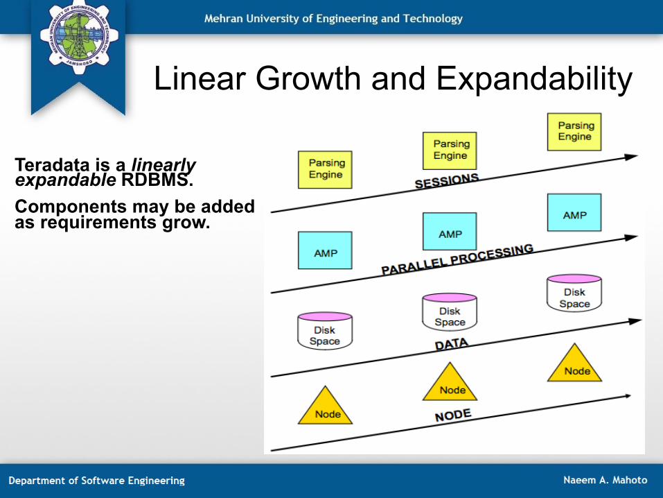
Linear Growth and Expandability

Teradata is a linearly expandable RDBMS. Components may be added as requirements grow.

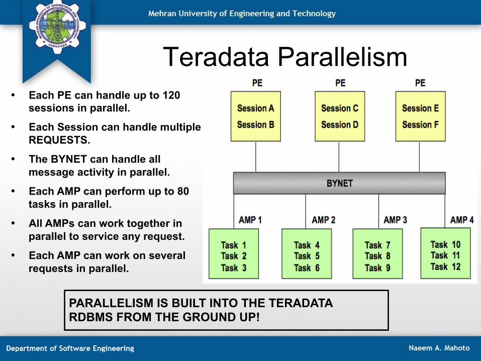
Teradata Parallelism •  Each PE can handle up to 120

sessions in parallel.

•  Each Session can handle multiple REQUESTS.

•  The BYNET can handle all message activity in parallel.

•  Each AMP can perform up to 80 tasks in parallel.

•  All AMPs can work together in parallel to service any request.

•  Each AMP can work on several requests in parallel.

PARALLELISM IS BUILT INTO THE TERADATA RDBMS FROM THE GROUND UP!

Teradata Functional Overview

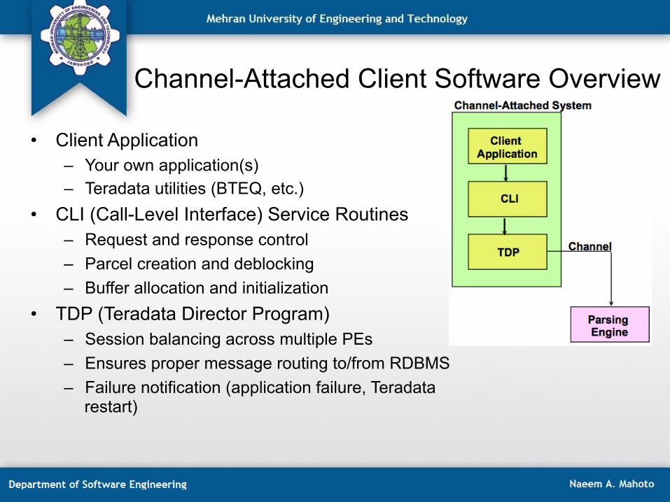
Channel-Attached Client Software Overview

•  Client Application –  Your own application(s) –  Teradata utilities (BTEQ, etc.)

•  CLI (Call-Level Interface) Service Routines –  Request and response control –  Parcel creation and deblocking –  Buffer allocation and initialization

•  TDP (Teradata Director Program) –  Session balancing across multiple PEs –  Ensures proper message routing to/from RDBMS –  Failure notification (application failure, Teradata

restart)

Network-Attached Client Software Overview

CLI (Call Level Interface) •  Library of routines for blocking/unblocking requests

and responses to/from the RDBMS MTDP (Micro Teradata Director Program) •  Library of session management routines MOSI (Micro Operating System Interface) •  Library of routines providing OS-independent

interface

Teradata Objects •  Three fundamental objects may be

found in a Teradata database: •  Tables—rows and columns of data •  Views—predefined subsets of existing

tables •  Macros—predefined, stored SQL

statements •  These objects are created, maintained,

and deleted using Structured Query Language (SQL).

•  Object definitions are stored in the Data Dictionary (DD).

The Data Dictionary (DD) •  The Data Dictionary (DD)

–  Is an integrated set of system tables. –  Contains definitions of and information about all objects in the

system. –  Is entirely maintained by the RDBMS. –  Is “data about the data” or “metadata.” –  Is distributed across all AMPs. –  May be queried by administrators or support staff. –  Is accessed via Teradata-supplied views.

•  Examples of views: –  DBC.Tables—information about all tables –  DBC.Users—information about all users –  DBC.AllRights—information about access rights –  DBC.DiskSpace—info about space utilization

Evolution of Data Processing Traditional

OLTP—On-line Transaction Processing Example: Update a checking account to reflect a deposit.

Small number of rows accessed Response time in seconds

DSS—Decision Support Systems Example: How many child size blue jeans were sold across all of our Eastern stores in the month of March?

Large number of rows processed Response time in seconds or minutes

Evolution of Data Processing Today

OLCP—On-line Complex Processing Example: Instant credit—How much credit can be extended to this person?

Small to moderate number of rows processed against multiple databases Response time in minutes

OLAP—On-line Analytical Processing Example: Show the top ten selling items across all stores for 1997.

Large number of detail rows or moderate number of summary rows processed Data aggregated and analyzed Response time in seconds or minutes

Data Protection: Locks

•  Exclusive—prevents any other type of concurrent access

•  Write—prevents other Read, Write, Exclusive locks

•  Read—prevents Write and Exclusive locks

•  Access—prevents Exclusive locks only

•  Database—applies to all tables/views in the database

•  Table/View—applies to all rows in the table/views

•  Row Hash—applies to all rows with same row hash

There are four types of locks:

Locks may be applied at three database levels:

Data Protection: Locks

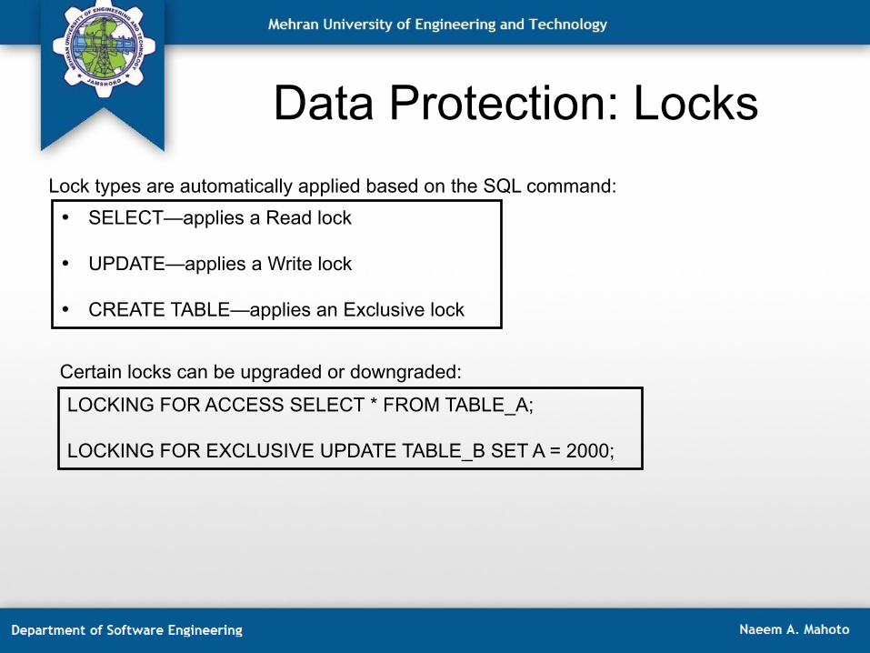
LOCKING FOR ACCESS SELECT * FROM TABLE_A; LOCKING FOR EXCLUSIVE UPDATE TABLE_B SET A = 2000;

Lock types are automatically applied based on the SQL command: •  SELECT—applies a Read lock

•  UPDATE—applies a Write lock

•  CREATE TABLE—applies an Exclusive lock

Certain locks can be upgraded or downgraded:

Rules of Locking

Lock requests are queued behind all outstanding incompatible lock requests for the same object.

Rule

LOCK LEVEL HELDLOCKREQUEST

ACCESS

READ

WRITE

EXCLUSIVE

NONE ACCESS READ WRITE EXCLUSIVE

Granted

Granted Granted

GrantedGranted

Granted

Granted

Granted

Granted Granted Queued

QueuedQueued

Queued

Queued

Queued

Queued

QueuedQueuedQueued

Queued

Example: Rules of Locking Example 1: A new READ lock request goes to the end of queue.

READ

WRITE READ READ WRITE READ

New request

New lock queue Lock queue Current lock Current lock

Example 2: A new READ lock request shares slot in the queue.

READ

READ WRITE READ WRITE

New request New lock queue

Lock Queue Current lock Current lock READ

Access Locks

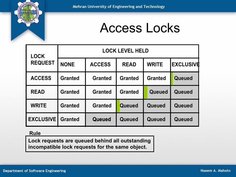
Lock requests are queued behind all outstanding incompatible lock requests for the same object.

Rule

LOCK LEVEL HELDLOCKREQUEST

ACCESS

READ

WRITE

EXCLUSIVE

NONE ACCESS READ WRITE EXCLUSIVE

Granted

Granted Granted

GrantedGranted

Granted

Granted

Granted

Granted Granted Queued

QueuedQueued

Queued

Queued

Queued

Queued

QueuedQueuedQueued

Queued

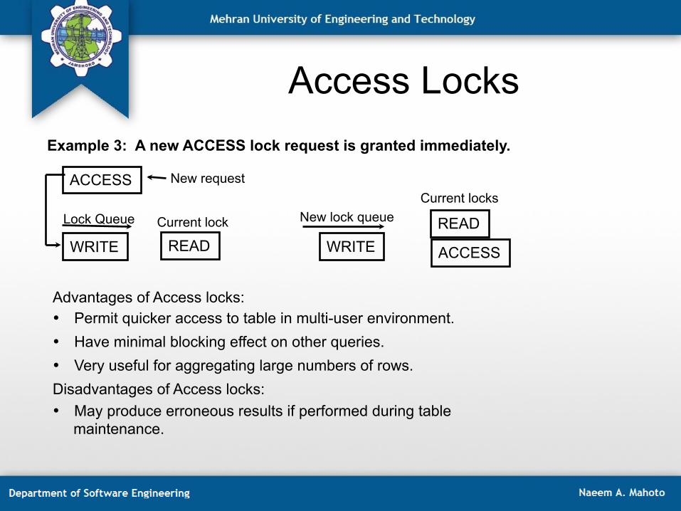
Access Locks Example 3: A new ACCESS lock request is granted immediately.

ACCESS

WRITE READ WRITE READ

New request

New lock queue Lock Queue Current lock

Current locks

ACCESS

Advantages of Access locks: •  Permit quicker access to table in multi-user environment. •  Have minimal blocking effect on other queries. •  Very useful for aggregating large numbers of rows. Disadvantages of Access locks: •  May produce erroneous results if performed during table

maintenance.

Fallback

Primary rows

PE PE

AMP 4 AMP 3 AMP 2 AMP 1

6 11 12 2 5 8 3 1

6 11 12 2 5 8 3 1

BYNET

Fallback rows

•  A fallback table is fully available in the event of an unavailable AMP. •  A fallback row is a copy of a primary row stored on a different AMP.

Note: The loss of two AMPs within a cluster will cause the RDBMS to halt!

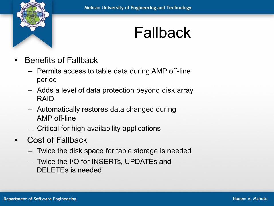
Fallback •  Benefits of Fallback

–  Permits access to table data during AMP off-line period

–  Adds a level of data protection beyond disk array RAID

–  Automatically restores data changed during AMP off-line

–  Critical for high availability applications

•  Cost of Fallback –  Twice the disk space for table storage is needed –  Twice the I/O for INSERTs, UPDATEs and

DELETEs is needed

Fallback Clustering –  A fallback cluster is a defined number of AMPs which are treated as a single, fault-

tolerant unit. –  All fallback rows for AMPs in a cluster must reside within

the cluster. –  Loss of one AMP in the cluster permits continued table access. –  Loss of two AMPs in the cluster causes the RDBMS to halt.

Two Clusters of Four AMPs Each

1 14 38 22 34 50 8 27 62 5 19 78

7 41 66 17 37 72 2 45 88 20 58 93

AMP 1 AMP 2 AMP 3 AMP 4

AMP 5 AMP 6 AMP 7 AMP 8

8 62 22 34 5 19 27 50 78 1 14 38

17 37 72 2 45 88 20 58 93 7 41 66

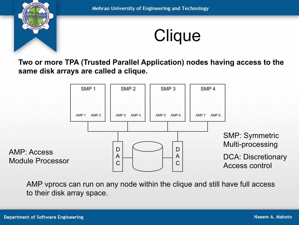
Clique Two or more TPA (Trusted Parallel Application) nodes having access to the same disk arrays are called a clique.

SMP 1 SMP 2 SMP 3 SMP 4

AMP 1 AMP 2 AMP 3 AMP 4 AMP 5 AMP 6 AMP 7 AMP 8

D A C

D A C

AMP vprocs can run on any node within the clique and still have full access to their disk array space.

SMP: Symmetric Multi-processing

DCA: Discretionary Access control

AMP: Access Module Processor

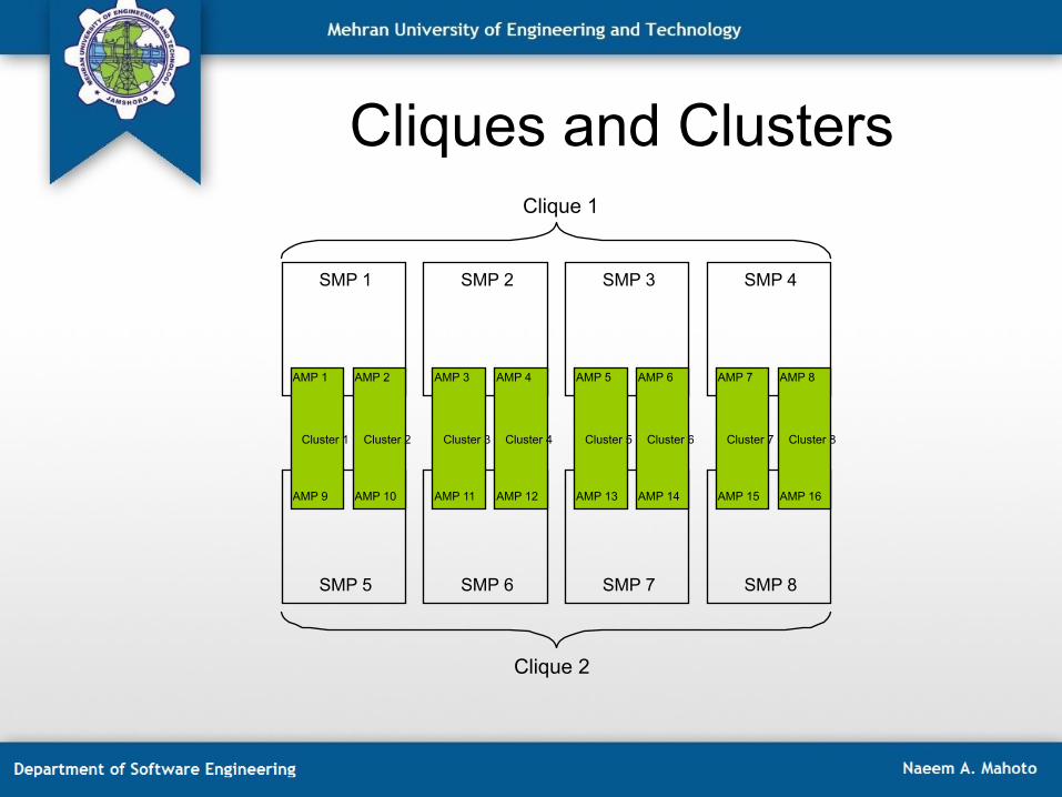
Cliques and Clusters

SMP 1 SMP 2 SMP 3 SMP 4

Clique 1

SMP 5

Cluster 2 Cluster 1

AMP 1 AMP 2

AMP 9 AMP 10

SMP 6 SMP 7 SMP 8

Cluster 4 Cluster 3

AMP 3 AMP 4

AMP 11 AMP 12

Cluster 6 Cluster 5

AMP 5 AMP 6

AMP 13 AMP 14

Cluster 8 Cluster 7

AMP 7 AMP 8

AMP 15 AMP 16

Clique 2