Data Mining Techniques for Query Relaxation

2

Query Relaxation via Abstraction

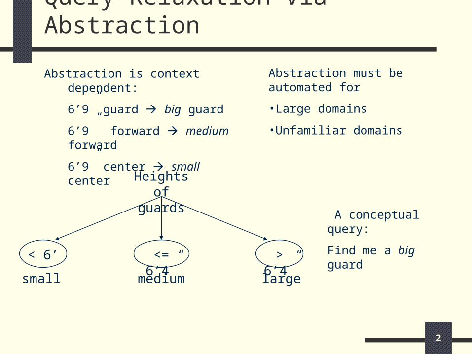
Abstraction is context dependent:

6’9” guard big guard

6’9” forward medium forward

6’9” center small center

< 6’ <= 6’4”

> 6’4”

small medium

large

Heights of

guards A conceptual query:

Find me a big guard

Abstraction must be automated for

•Large domains

•Unfamiliar domains

3

Related Work

Maximum Entropy (ME) method: Maximization of entropy (- p log p) Only considers frequency distribution

Conceptual clustering systems: Only allows non-numerical values (COBWEB) Assume a certain distribution (CLASSIT)

4

Supervised vs. Unsupervised LearningSupervised Learning:Given instances with known class information,

generate rules/decision tree that can be used to infer class of future instances

Examples: ID3, Statistical Pattern Recognition

Unsupervised Learning:Given instances with unknown class information,

generate concept tree that cluster instances into similar classes

Examples: COBWEB, TAH Generation (DISC, PBKI)

5

Automatic Construction of TAHs

Necessary for Scaling up CoBaseSources of Knowledge Database Instance

Attribute Value Distributions Inter-Attribute Relationships

Query and Answer Statistics Domain Expert

Approach Generate Initial TAH

With Minimal Expert Effort Edit the Hierarchy to Suit

Application Context User Profile

For Clustering Attribute Instances with Non-Numerical

Values

7

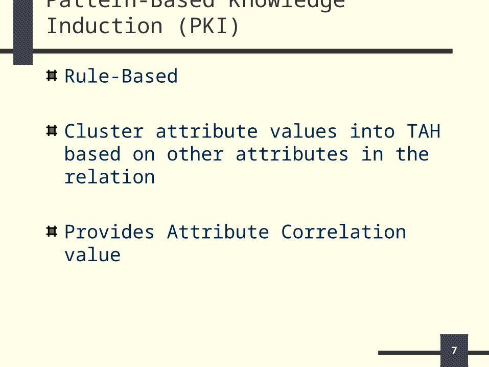
Pattern-Based Knowledge Induction (PKI)

Rule-Based

Cluster attribute values into TAH based on other attributes in the relation

Provides Attribute Correlation value

8

Definitions

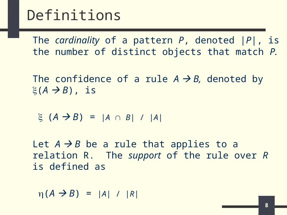
The cardinality of a pattern P, denoted |P|, is the number of distinct objects that match P.

The confidence of a rule A B, denoted by (A B), is

(A B) = |A B| / |A|

Let A B be a rule that applies to a relation R. The support of the rule over R is defined as

(A B) = |A| / |R|

9

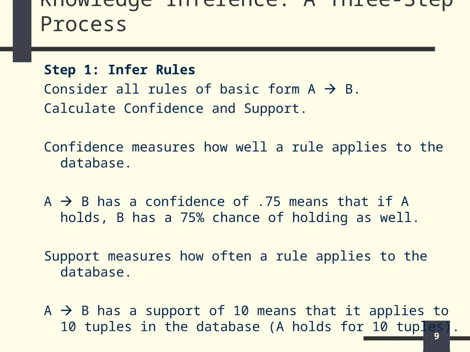
Knowledge Inference: A Three-Step Process

Step 1: Infer RulesConsider all rules of basic form A B.Calculate Confidence and Support.

Confidence measures how well a rule applies to the database.

A B has a confidence of .75 means that if A holds, B has a 75% chance of holding as well.

Support measures how often a rule applies to the database.

A B has a support of 10 means that it applies to 10 tuples in the database (A holds for 10 tuples).

10

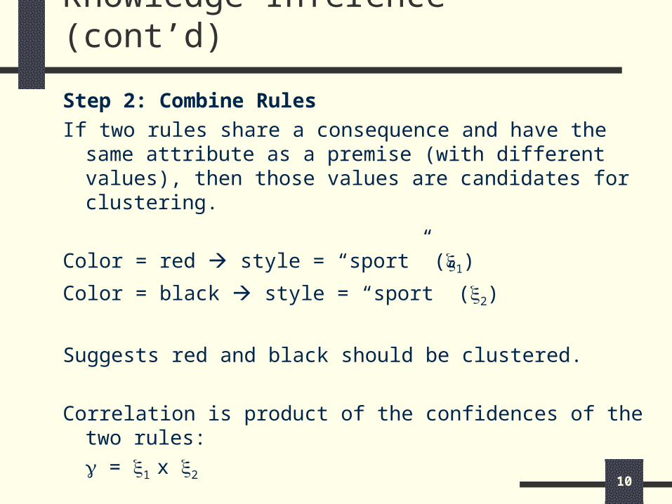
Knowledge Inference (cont’d)

Step 2: Combine RulesIf two rules share a consequence and have the same

attribute as a premise (with different values), then those values are candidates for clustering.

Color = red style = “sport” (1)

Color = black style = “sport” (2)

Suggests red and black should be clustered.

Correlation is product of the confidences of the two rules:

= 1 x 2

11

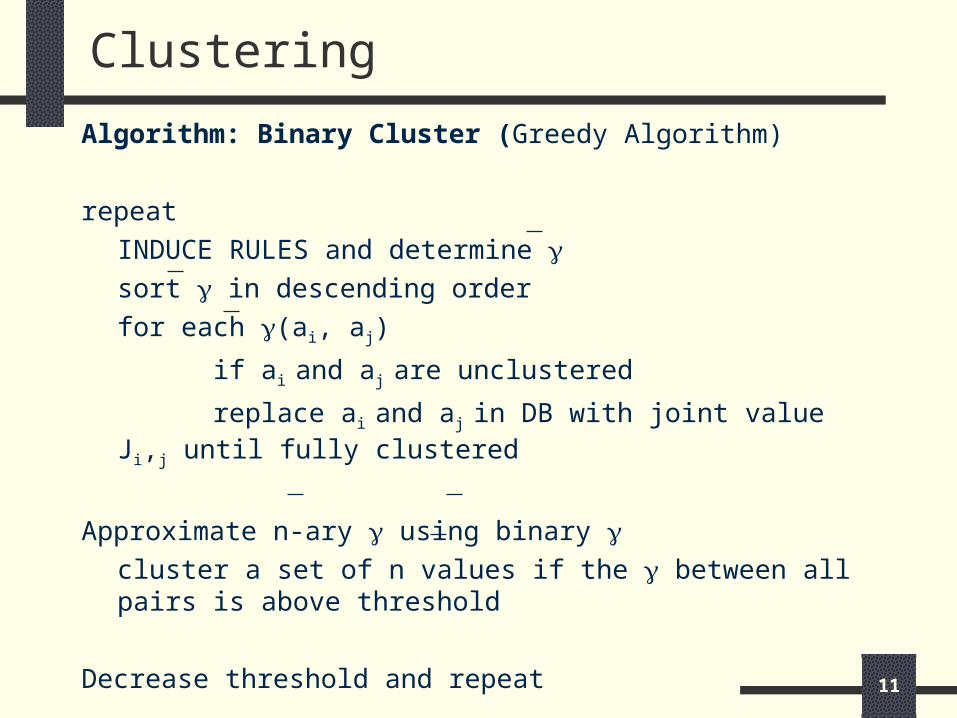
Clustering

Algorithm: Binary Cluster (Greedy Algorithm)

repeatINDUCE RULES and determine sort in descending orderfor each (ai, aj)

if ai and aj are unclustered

replace ai and aj in DB with joint value Ji,j until fully clustered

Approximate n-ary using binary cluster a set of n values if the between all pairs is above threshold

Decrease threshold and repeat

12

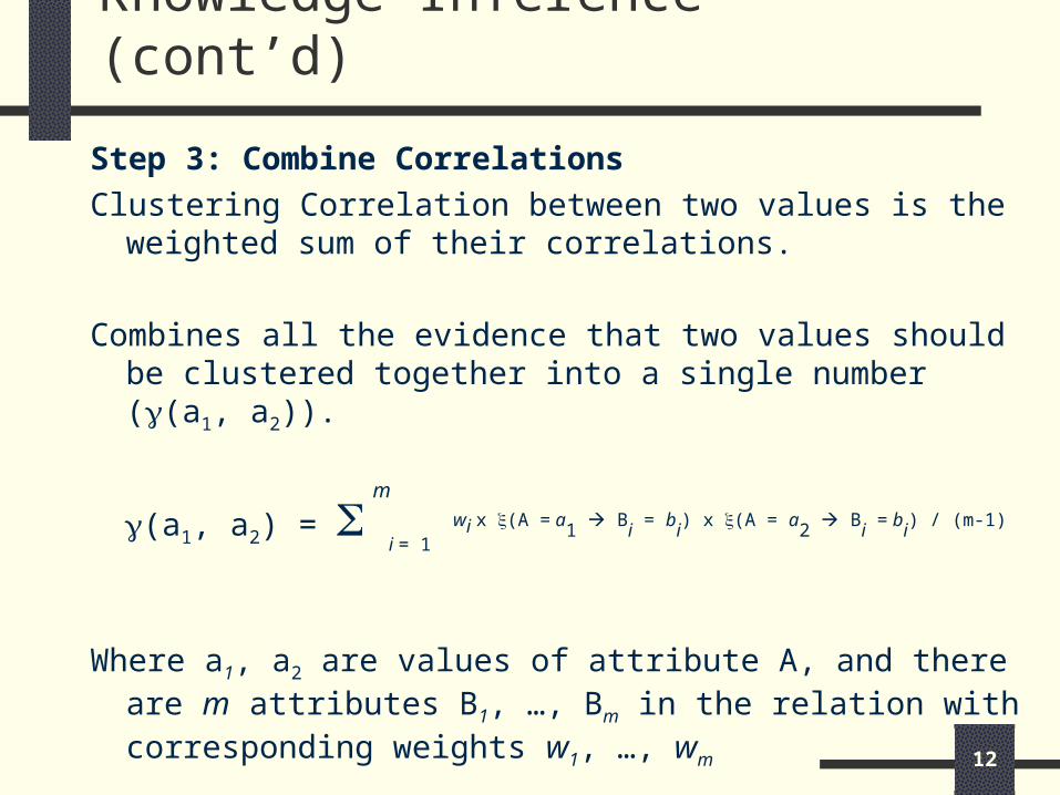
Knowledge Inference (cont’d)

Step 3: Combine CorrelationsClustering Correlation between two values is the

weighted sum of their correlations.

Combines all the evidence that two values should be clustered together into a single number ((a1, a2)).

(a1, a2) = i = 1

wi x (A = a

1 B

i = b

i) x (A = a

2 B

i = b

i) / (m-1)

Where a1, a2 are values of attribute A, and there are m attributes B1, …, Bm in the relation with corresponding weights w1, …, wm

m

13

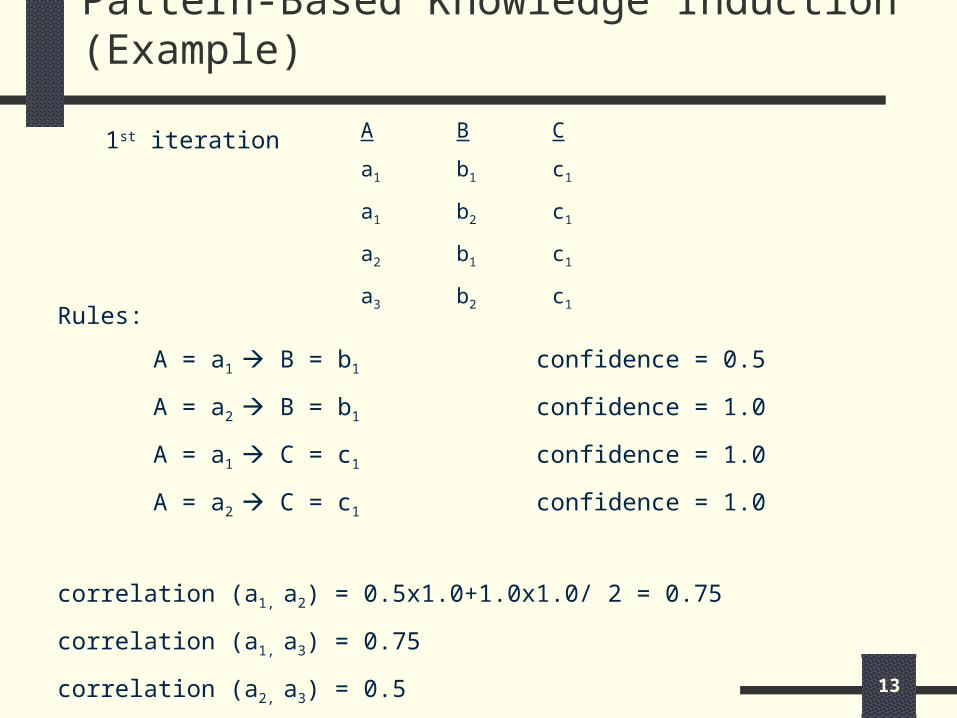
Pattern-Based Knowledge Induction (Example)

A B C

a1 b1 c1

a1 b2 c1

a2 b1 c1

a3 b2 c1Rules:

A = a1 B = b1 confidence = 0.5

A = a2 B = b1 confidence = 1.0

A = a1 C = c1 confidence = 1.0

A = a2 C = c1 confidence = 1.0

correlation (a1, a2) = 0.5x1.0+1.0x1.0/ 2 = 0.75

correlation (a1, a3) = 0.75

correlation (a2, a3) = 0.5

1st iteration

14

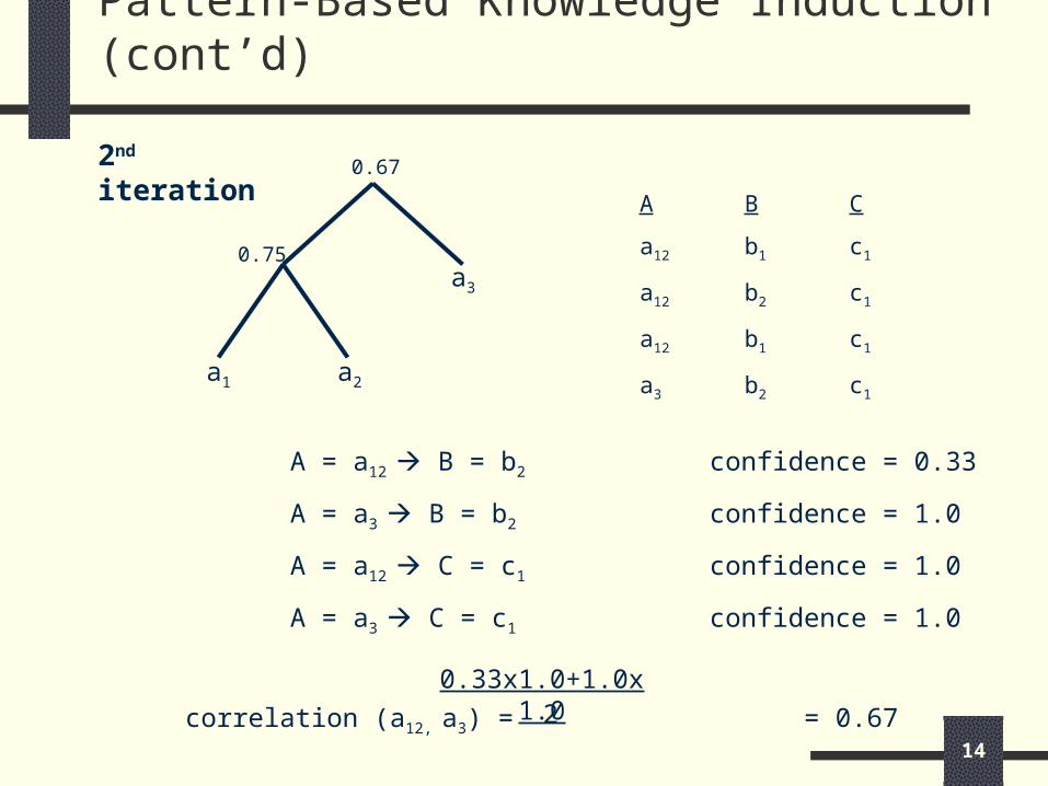
Pattern-Based Knowledge Induction (cont’d)

A B C

a12 b1 c1

a12 b2 c1

a12 b1 c1

a3 b2 c1

A = a12 B = b2 confidence = 0.33

A = a3 B = b2 confidence = 1.0

A = a12 C = c1 confidence = 1.0

A = a3 C = c1 confidence = 1.0

correlation (a12, a3) = = 0.67

0.33x1.0+1.0x1.02

a1 a2

a3

0.67

0.75

2nd iteration

15

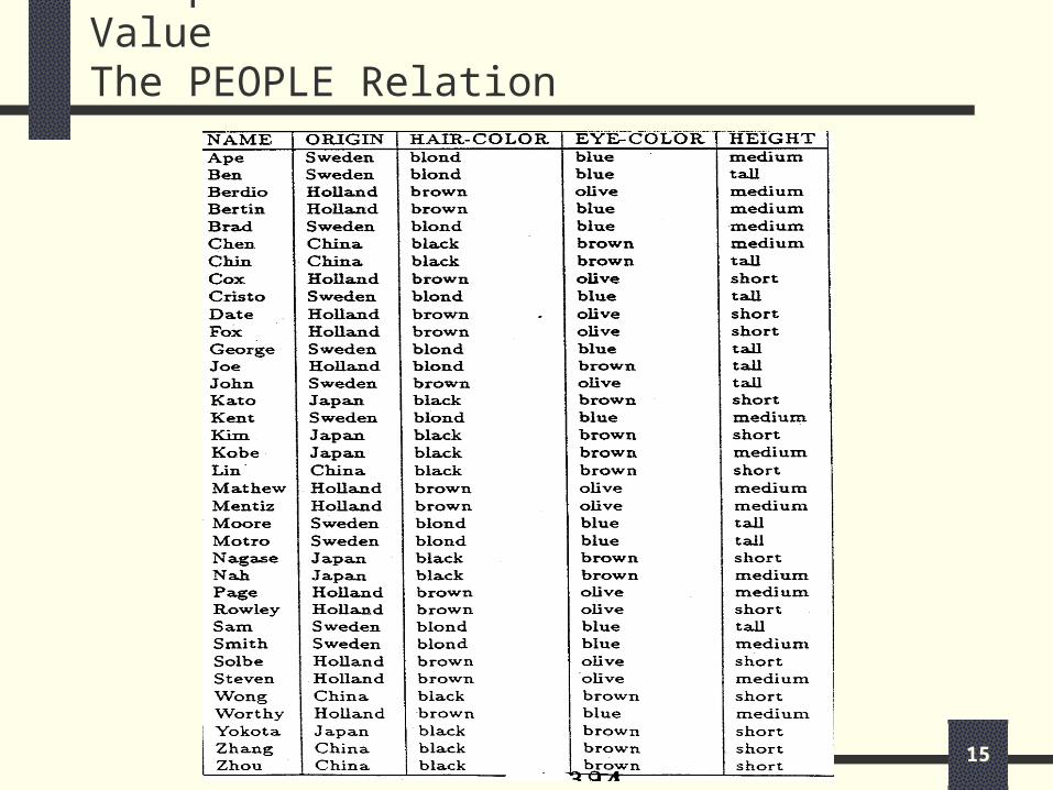
Example for Non-Numerical Attribute ValueThe PEOPLE Relation

16

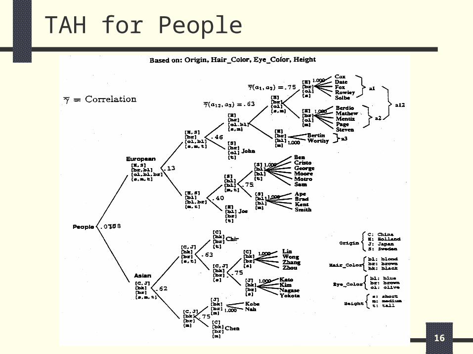
TAH for People

17

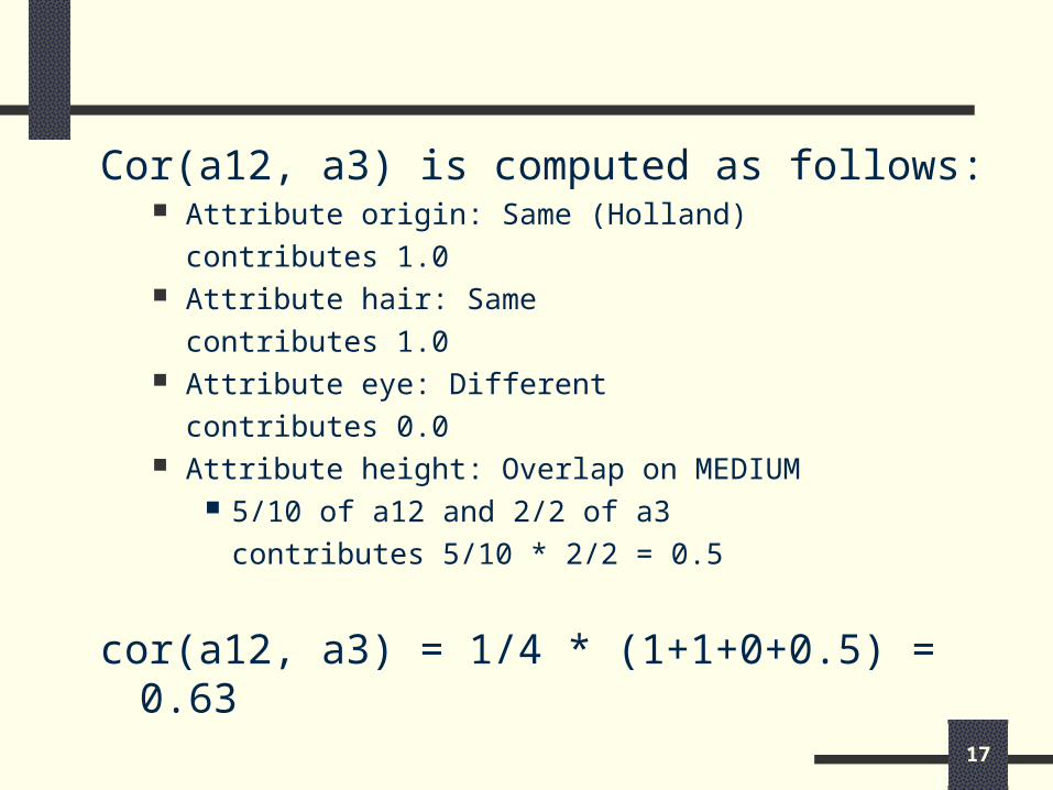
Cor(a12, a3) is computed as follows: Attribute origin: Same (Holland)

contributes 1.0 Attribute hair: Same

contributes 1.0 Attribute eye: Different

contributes 0.0 Attribute height: Overlap on MEDIUM

5/10 of a12 and 2/2 of a3contributes 5/10 * 2/2 = 0.5

cor(a12, a3) = 1/4 * (1+1+0+0.5) = 0.63

18

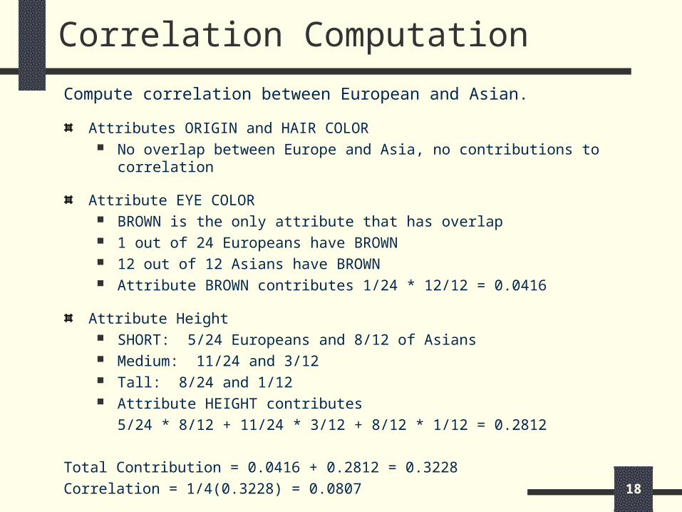
Correlation Computation

Compute correlation between European and Asian.

Attributes ORIGIN and HAIR COLOR No overlap between Europe and Asia, no contributions to correlation

Attribute EYE COLOR BROWN is the only attribute that has overlap 1 out of 24 Europeans have BROWN 12 out of 12 Asians have BROWN Attribute BROWN contributes 1/24 * 12/12 = 0.0416

Attribute Height SHORT: 5/24 Europeans and 8/12 of Asians Medium: 11/24 and 3/12 Tall: 8/24 and 1/12 Attribute HEIGHT contributes

5/24 * 8/12 + 11/24 * 3/12 + 8/12 * 1/12 = 0.2812

Total Contribution = 0.0416 + 0.2812 = 0.3228Correlation = 1/4(0.3228) = 0.0807

19

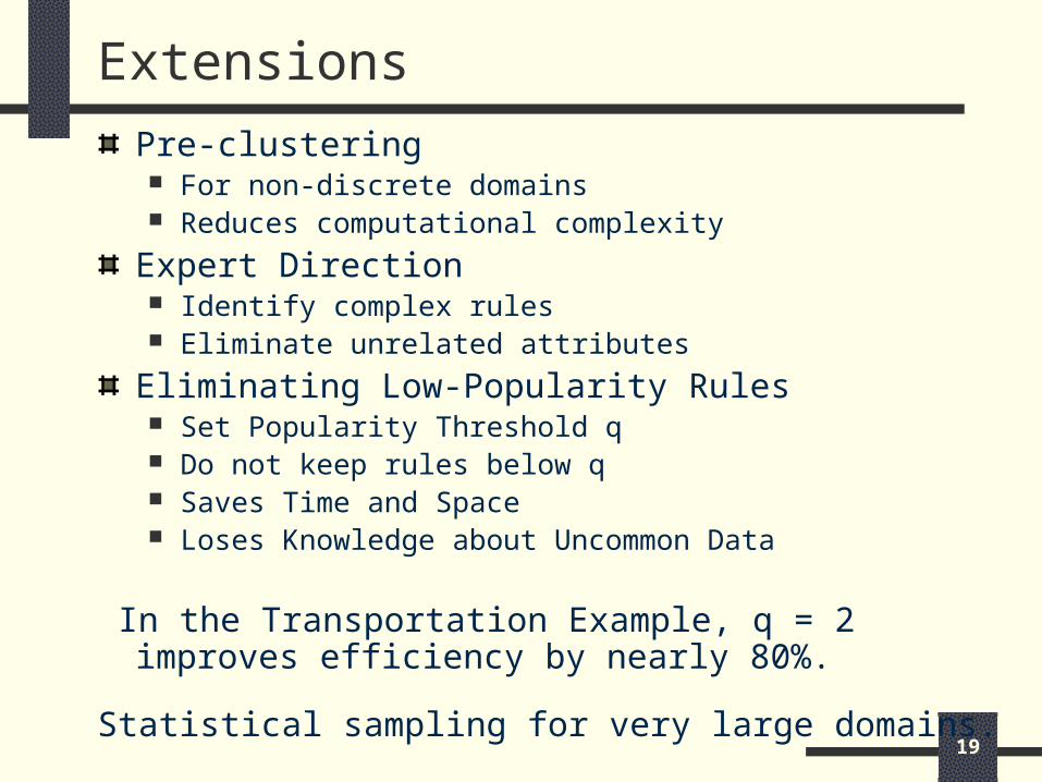
Extensions

Pre-clustering For non-discrete domains Reduces computational complexity

Expert Direction Identify complex rules Eliminate unrelated attributes

Eliminating Low-Popularity Rules Set Popularity Threshold q Do not keep rules below q Saves Time and Space Loses Knowledge about Uncommon Data

In the Transportation Example, q = 2 improves efficiency by nearly 80%.

Statistical sampling for very large domains.

Clustering of Attribute Instances with Numerical

Values

21

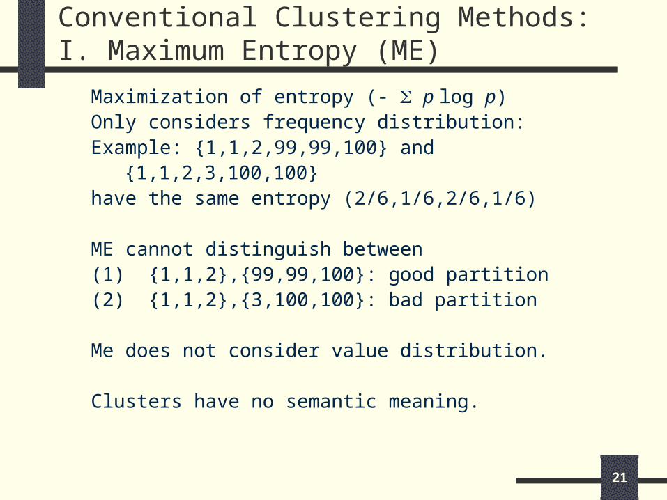
Conventional Clustering Methods:I. Maximum Entropy (ME)

Maximization of entropy (- p log p)Only considers frequency distribution:Example: {1,1,2,99,99,100} and

{1,1,2,3,100,100}have the same entropy (2/6,1/6,2/6,1/6)

ME cannot distinguish between(1) {1,1,2},{99,99,100}: good partition(2) {1,1,2},{3,100,100}: bad partition

Me does not consider value distribution.

Clusters have no semantic meaning.

22

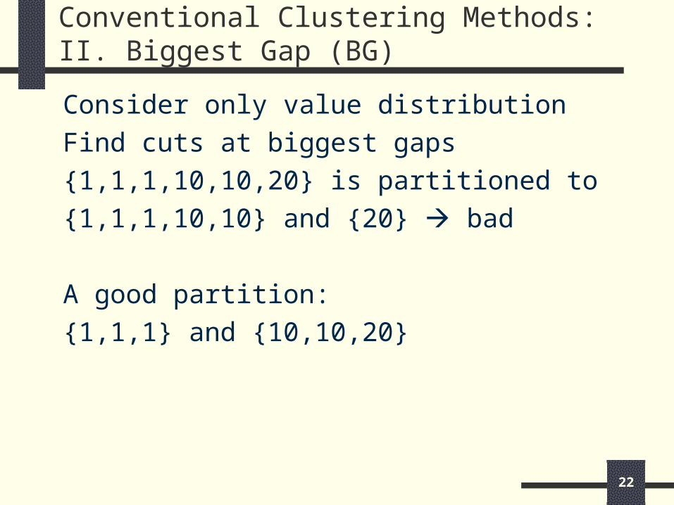
Conventional Clustering Methods:II. Biggest Gap (BG)

Consider only value distributionFind cuts at biggest gaps{1,1,1,10,10,20} is partitioned to{1,1,1,10,10} and {20} bad

A good partition:{1,1,1} and {10,10,20}

23

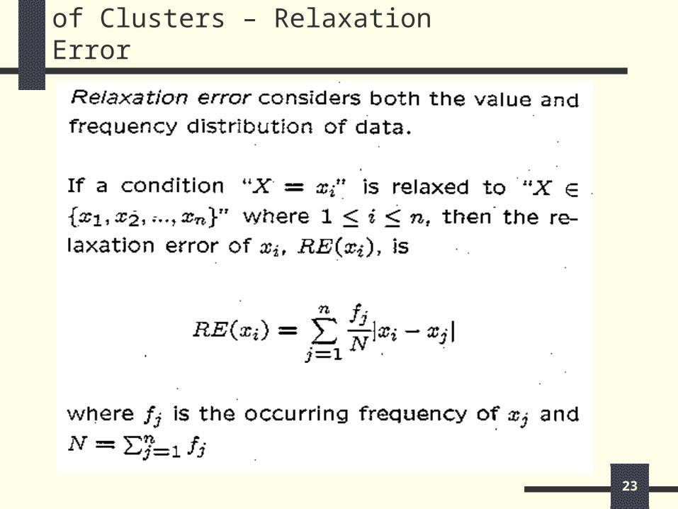
New Notion of “Goodness” of Clusters – Relaxation Error

24

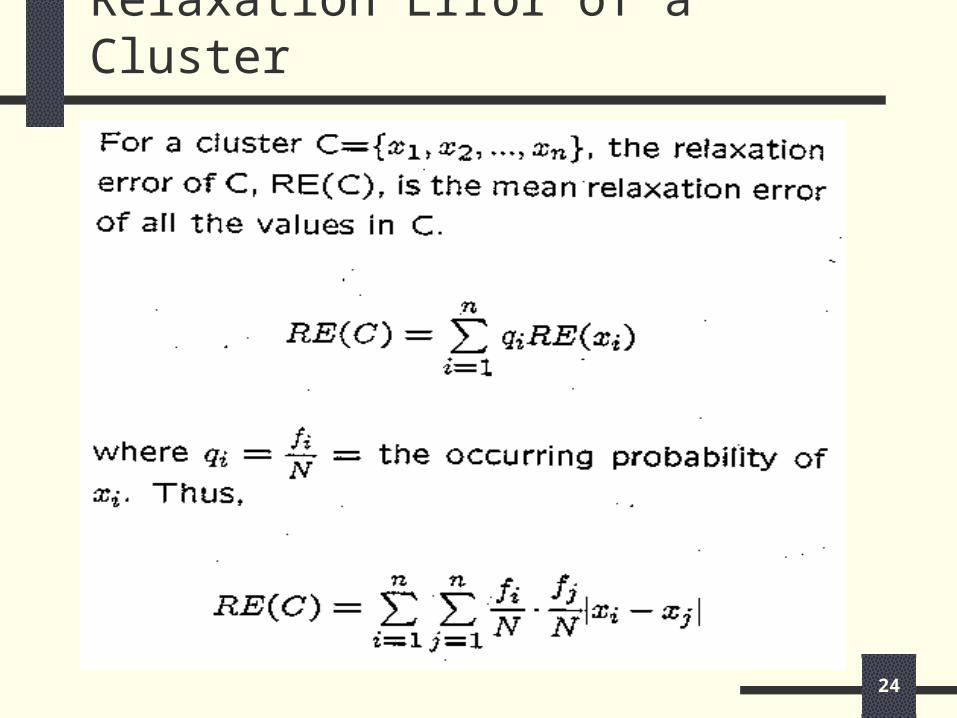
Relaxation Error of a Cluster

25

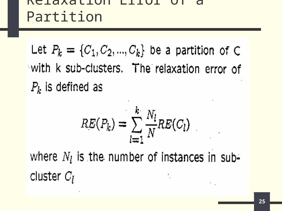
Relaxation Error of a Partition

26

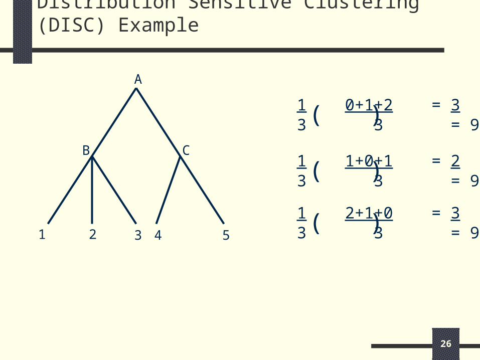
Distribution Sensitive Clustering (DISC) Example

A

B C

1 2 3 4 5

1 0+1+2 = 33 3 = 9( )

1 1+0+1 = 23 3 = 9( )

1 2+1+0 = 33 3 = 9( )

27

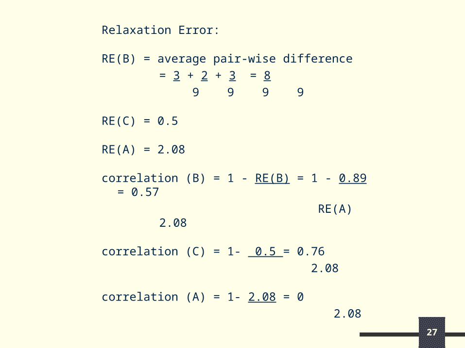
Relaxation Error:

RE(B) = average pair-wise difference

= 3 + 2 + 3 = 8

9 9 9 9

RE(C) = 0.5

RE(A) = 2.08

correlation (B) = 1 - RE(B) = 1 - 0.89 = 0.57

RE(A) 2.08

correlation (C) = 1- 0.5 = 0.76

2.08

correlation (A) = 1- 2.08 = 0

2.08

28

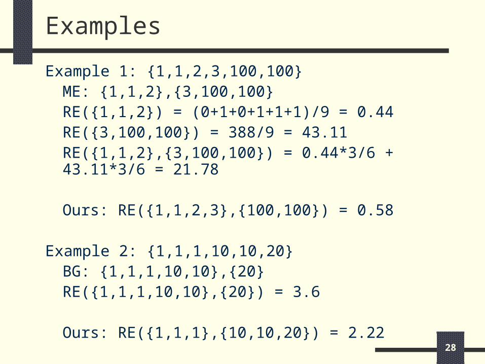
Examples

Example 1: {1,1,2,3,100,100}ME: {1,1,2},{3,100,100}RE({1,1,2}) = (0+1+0+1+1+1)/9 = 0.44RE({3,100,100}) = 388/9 = 43.11RE({1,1,2},{3,100,100}) = 0.44*3/6 + 43.11*3/6 = 21.78

Ours: RE({1,1,2,3},{100,100}) = 0.58

Example 2: {1,1,1,10,10,20}BG: {1,1,1,10,10},{20}

RE({1,1,1,10,10},{20}) = 3.6

Ours: RE({1,1,1},{10,10,20}) = 2.22

29

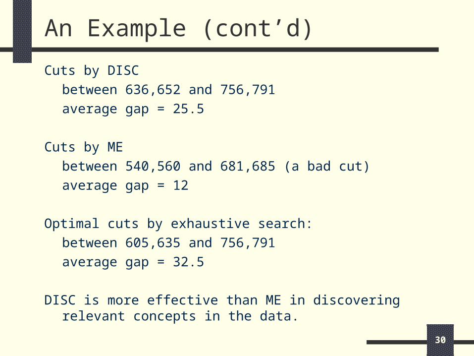
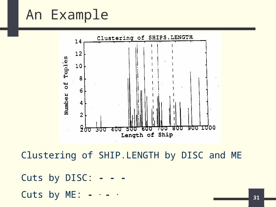
An Example

Example:

The table SHIPS has 153 tuples and the attribute LENGTH has 33 distinct values ranging from 273 to 947. DISC and ME are used to cluster LENGTH into three sub-concepts: SHORT, MEDIUM, and LONG.

30

An Example (cont’d)

Cuts by DISCbetween 636,652 and 756,791average gap = 25.5

Cuts by MEbetween 540,560 and 681,685 (a bad cut)average gap = 12

Optimal cuts by exhaustive search:between 605,635 and 756,791average gap = 32.5

DISC is more effective than ME in discovering relevant concepts in the data.

31

An Example

Clustering of SHIP.LENGTH by DISC and ME

Cuts by DISC: - - -

Cuts by ME: - . - .

32

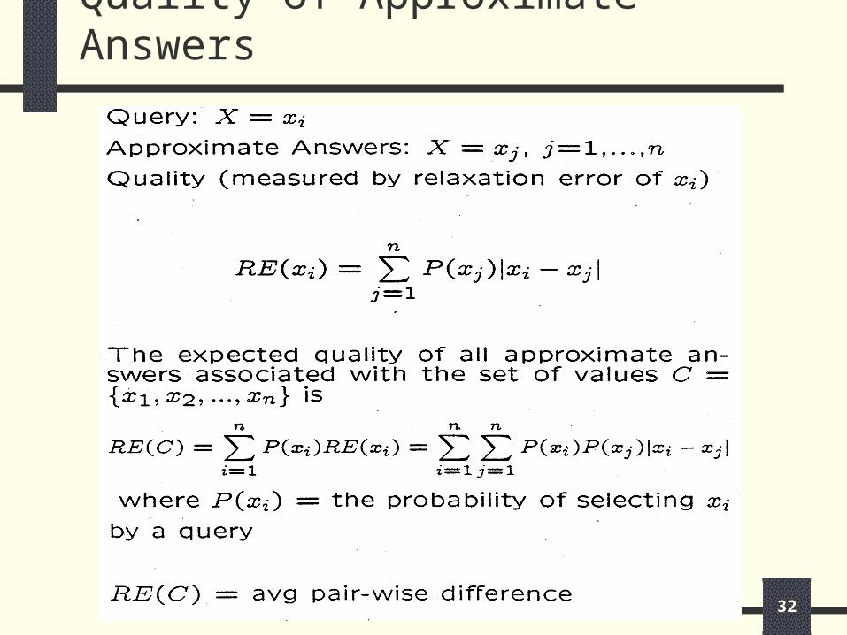
Quality of Approximate Answers

33

DISC

For numeric domainsUses intra-attribute knowledge

Sensitive to both frequency and value distributions of data.

RE = average difference between exact and approximate answers in a cluster.

Quality of approximate answers are measured by relaxation error (RE): the smaller the RE, the better the approximate answer.

DISC (Distribution Sensitive Clustering) generates AAHs based on minimization of RE.

34

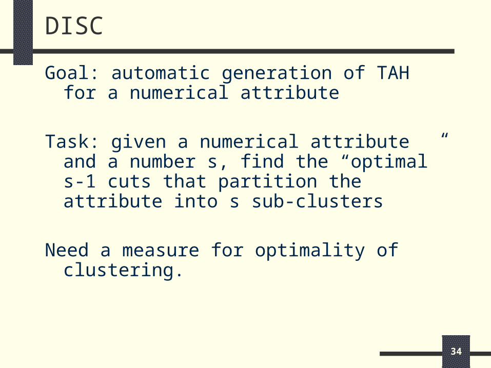
DISC

Goal: automatic generation of TAH for a numerical attribute

Task: given a numerical attribute and a number s, find the “optimal” s-1 cuts that partition the attribute into s sub-clusters

Need a measure for optimality of clustering.

35

Quality of Partitions

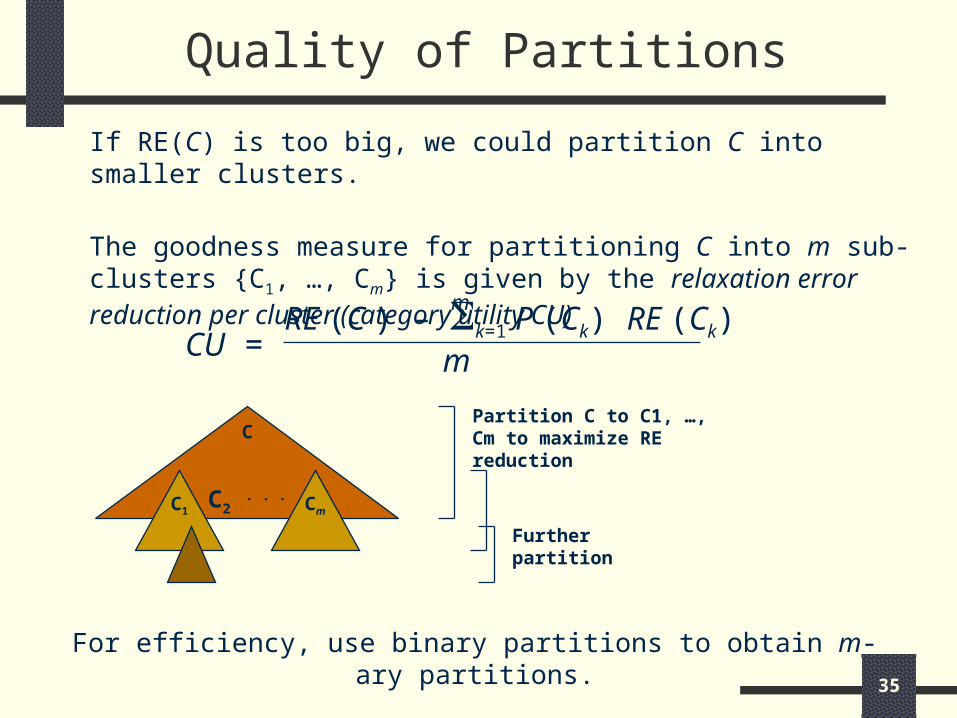
If RE(C) is too big, we could partition C into smaller clusters.

The goodness measure for partitioning C into m sub-clusters {C1, …, Cm} is given by the relaxation error reduction per cluster (category utility CU)

CU =

RE (C ) – k=1 P (Ck) RE (Ck)m

m

For efficiency, use binary partitions to obtain m-ary partitions.

C2 . . .C1 Cm

CPartition C to C1, …, Cm to maximize RE reduction

Further partition

36

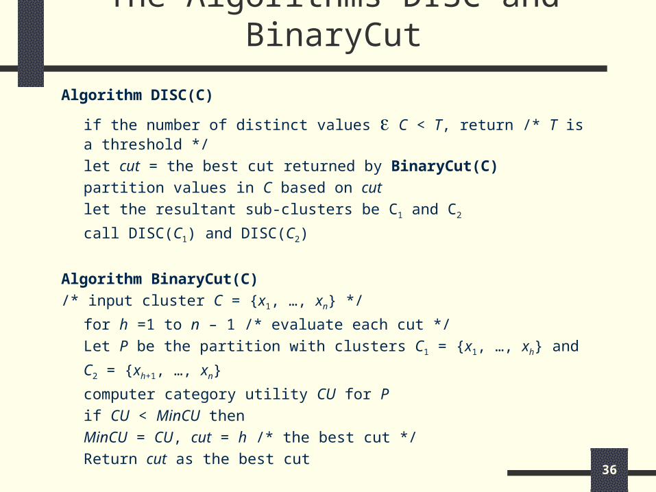
The Algorithms DISC and BinaryCut

Algorithm DISC(C)

if the number of distinct values C < T, return /* T is a threshold */

let cut = the best cut returned by BinaryCut(C)

partition values in C based on cut

let the resultant sub-clusters be C1 and C2

call DISC(C1) and DISC(C2)

Algorithm BinaryCut(C)

/* input cluster C = {x1, …, xn} */

for h =1 to n – 1 /* evaluate each cut */

Let P be the partition with clusters C1 = {x1, …, xh} and

C2 = {xh+1, …, xn}

computer category utility CU for P

if CU < MinCU then

MinCU = CU, cut = h /* the best cut */

Return cut as the best cut

37

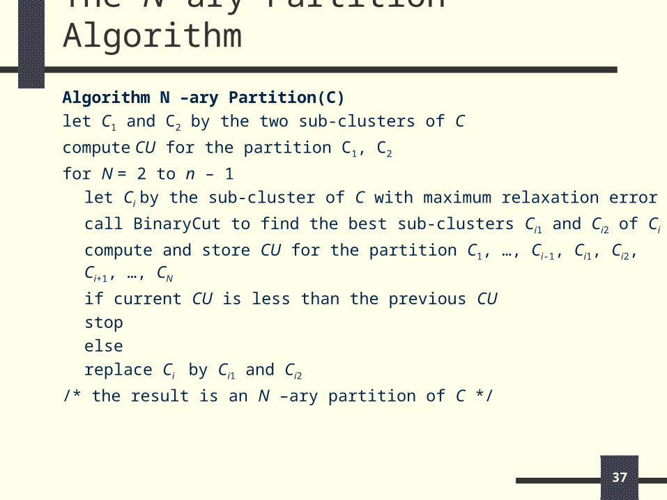
The N-ary Partition Algorithm

Algorithm N –ary Partition(C)let C1 and C2 by the two sub-clusters of C

compute CU for the partition C1, C2

for N = 2 to n – 1let Ci by the sub-cluster of C with maximum relaxation error

call BinaryCut to find the best sub-clusters Ci1 and Ci2 of Ci

compute and store CU for the partition C1, …, Ci-1, Ci1, Ci2, Ci+1, …, CN

if current CU is less than the previous CUstop

elsereplace Ci by Ci1 and Ci2

/* the result is an N –ary partition of C */

38

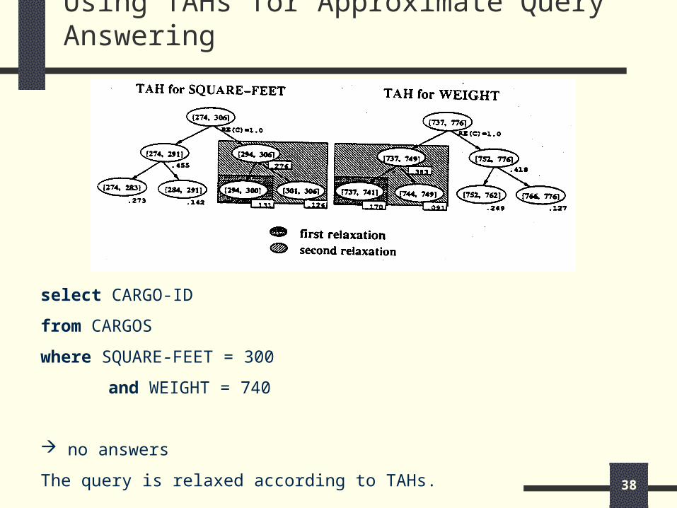
Using TAHs for Approximate Query Answering

select CARGO-ID

from CARGOS

where SQUARE-FEET = 300

and WEIGHT = 740

no answers

The query is relaxed according to TAHs.

39

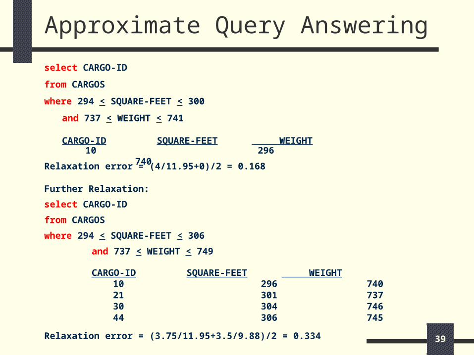
Approximate Query Answering

select CARGO-ID

from CARGOS

where 294 < SQUARE-FEET < 300

and 737 < WEIGHT < 741

CARGO-ID SQUARE-FEET WEIGHT 10 296 740

Relaxation error = (4/11.95+0)/2 = 0.168

Further Relaxation:

select CARGO-ID

from CARGOS

where 294 < SQUARE-FEET < 306

and 737 < WEIGHT < 749

CARGO-ID SQUARE-FEET WEIGHT 10 296 740 21 301 737 30 304 746 44 306 745

Relaxation error = (3.75/11.95+3.5/9.88)/2 = 0.334

40

Performance of DISC

Theorem: Let D and M be the optimal binary cuts by DISC and ME respectively. If the data distribution is symmetrical with respect to the median, then D = M (i.e., the cuts determined by DISC and ME are the same).

For skewed distributions, clusters discovered by DISC have less relaxation error than those by the ME method.

The more skewed the data, the greater the performance difference between DISC and ME.

41

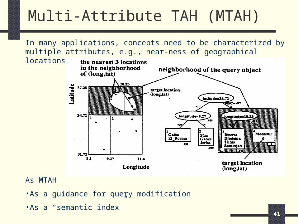
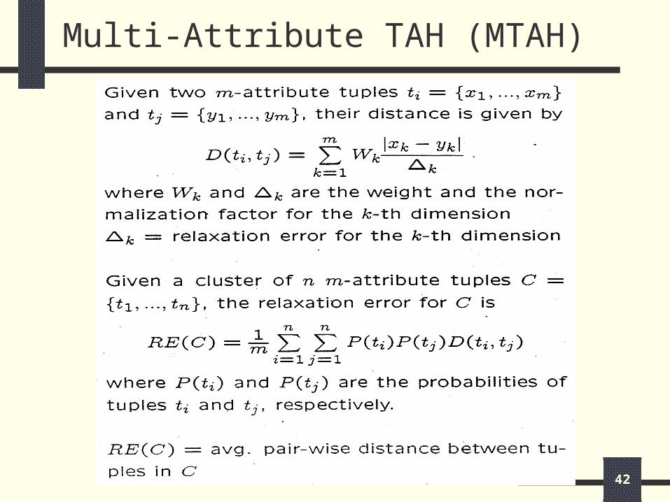
Multi-Attribute TAH (MTAH)

In many applications, concepts need to be characterized by multiple attributes, e.g., near-ness of geographical locations.

As MTAH

•As a guidance for query modification

•As a “semantic index”

42

Multi-Attribute TAH (MTAH)

43

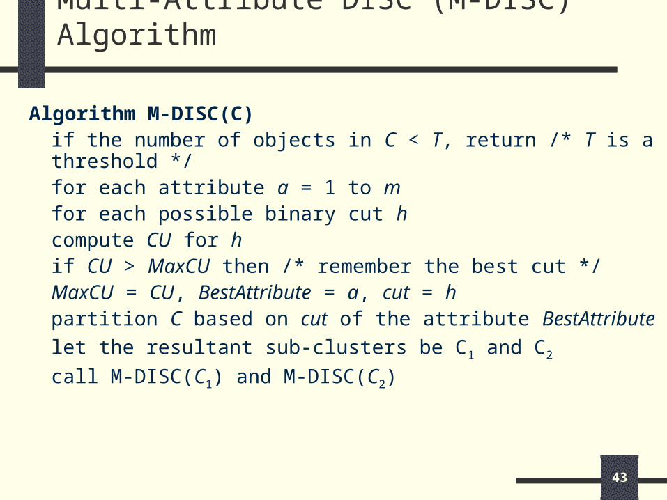
Multi-Attribute DISC (M-DISC) Algorithm

Algorithm M-DISC(C)if the number of objects in C < T, return /* T is a threshold */for each attribute a = 1 to m

for each possible binary cut hcompute CU for hif CU > MaxCU then /* remember the best cut */

MaxCU = CU, BestAttribute = a, cut = hpartition C based on cut of the attribute BestAttributelet the resultant sub-clusters be C1 and C2

call M-DISC(C1) and M-DISC(C2)

44

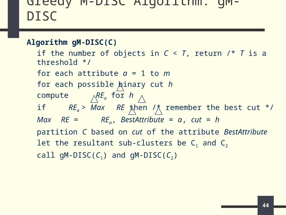
Greedy M-DISC Algorithm: gM-DISC

Algorithm gM-DISC(C)if the number of objects in C < T, return /* T is a threshold */for each attribute a = 1 to m

for each possible binary cut hcompute REa for h

if REa > Max RE then /* remember the best cut */

Max RE = REa, BestAttribute = a, cut = hpartition C based on cut of the attribute BestAttributelet the resultant sub-clusters be C1 and C2

call gM-DISC(C1) and gM-DISC(C2)

45

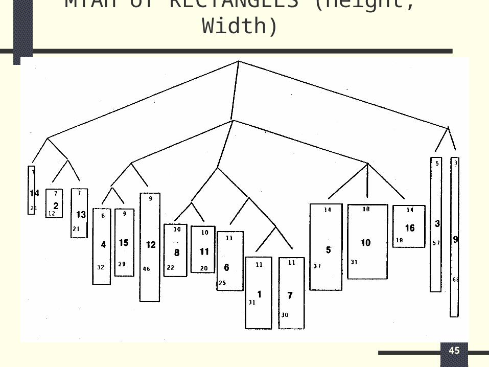
MTAH of RECTANGLES (Height, Width)

46

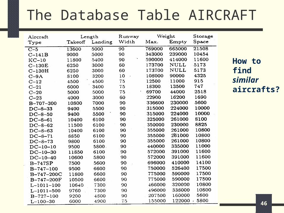
The Database Table AIRCRAFT

How to find similar aircrafts?

47

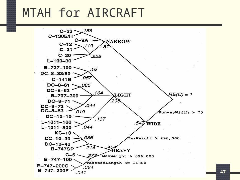
MTAH for AIRCRAFT

48

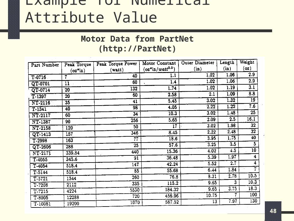
Example for Numerical Attribute Value

Motor Data from PartNet(http://PartNet)

49

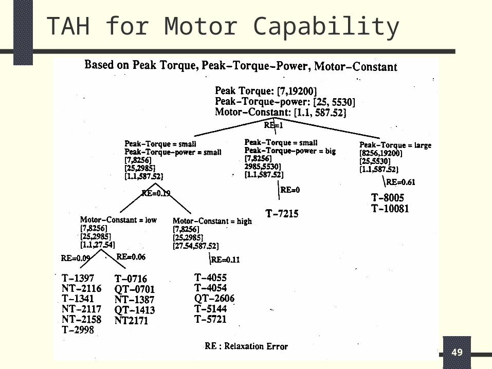
TAH for Motor Capability

50

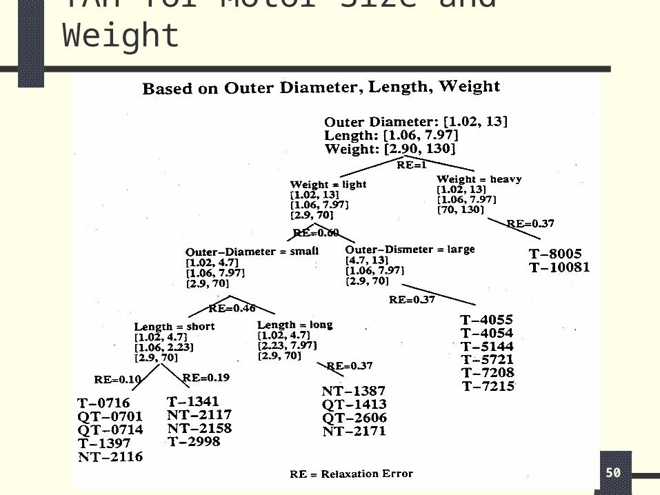
TAH for Motor Size and Weight

51

TAHs for Motor

The Motor table was adapted from Housed Torque from Part Net. After inputting the data, two TAHs were generated automatically from the DISC algorithm.

One TAH was based on peak torque, peak torque power, and motor constant. The other was based on outer diameter, length, and weight. The leaf nodes represent part number. THE intermediate nodes are classes. The relaxation error (average pair-wise distance between the parts) of each node are also given.

52

Application of TAHs

The TAHs can be used jointly to satisfy attributes in both TAHs. For example, find part similar to “T-0716” in terms of peak torque, peak torque power, motor constant, outer diameter, length, and weight. By examining both TAHs, we know that QT-0701 is similar to T-0716 with an expected relaxation error of (0.06 + 0.1)/2 = 0.08

53

Performance of TAH

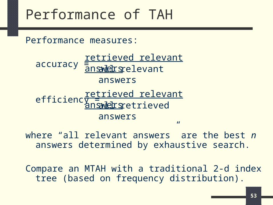
Performance measures:

accuracy =

efficiency =

where “all relevant answers” are the best n answers determined by exhaustive search.

Compare an MTAH with a traditional 2-d index tree (based on frequency distribution).

retrieved relevant answers

retrieved relevant answers

all relevant answers

all retrieved answers

54

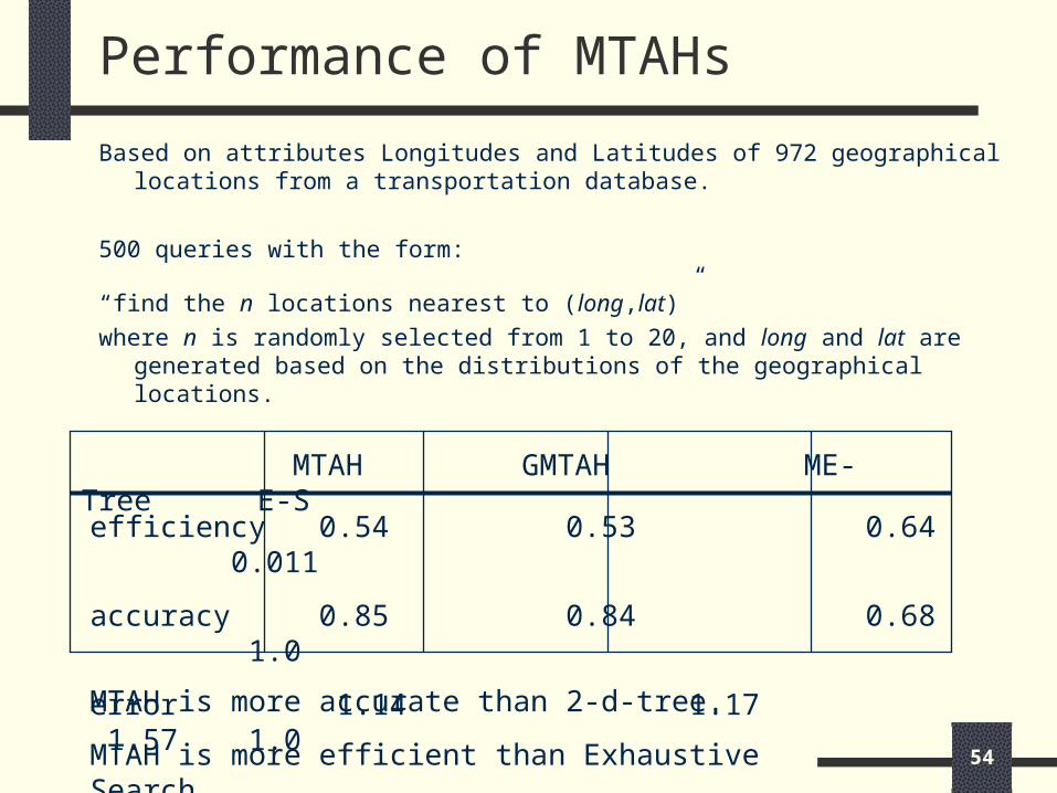
Performance of MTAHs

Based on attributes Longitudes and Latitudes of 972 geographical locations from a transportation database.

500 queries with the form:

“find the n locations nearest to (long,lat)”where n is randomly selected from 1 to 20, and long and lat are

generated based on the distributions of the geographical locations.

efficiency 0.54 0.53 0.64 0.011

accuracy 0.85 0.84 0.68 1.0

error 1.14 1.17 1.57 1.0

MTAH GMTAH ME-Tree E-S

MTAH is more accurate than 2-d-tree.

MTAH is more efficient than Exhaustive Search.

55

Generation of Evolutionary TAH

Approximate query answering for temporal data (given as a set of time sequences):

Find time sequences that are similar to a given template sequence.

A time sequence S of n stages is defined as an n-tuple: S = {s1, …, sn} where si is a numerical value.

Issues: Needs a similarity measure for sequences Use clustering for efficient retrieval Evaluation of work

56

Automatic Constructions of TAHs

Necessary for scaling up CoBaseSources of Knowledge Database Instance

Attribute Value Distributions Inter-Attribute Relationships

Query and Answer Statistics Domain Exert

Approach Generate Initial TAH

With Minimal Expert Effort Edit the Hierarchy to Suit

Application Context User Profile

57

The CoBase Knowledge-Base Editor

Tool for Type Abstraction Hierarchies Display available TAHs Visualize TAHs as graphs Edit TAHs

Add/Delete/Move nodes and sub-trees Assign names to nodes

Interface to Knowledge Discovery ToolsCooperative Operators Specify parameter values Approximate Near-To, Similar-To

58

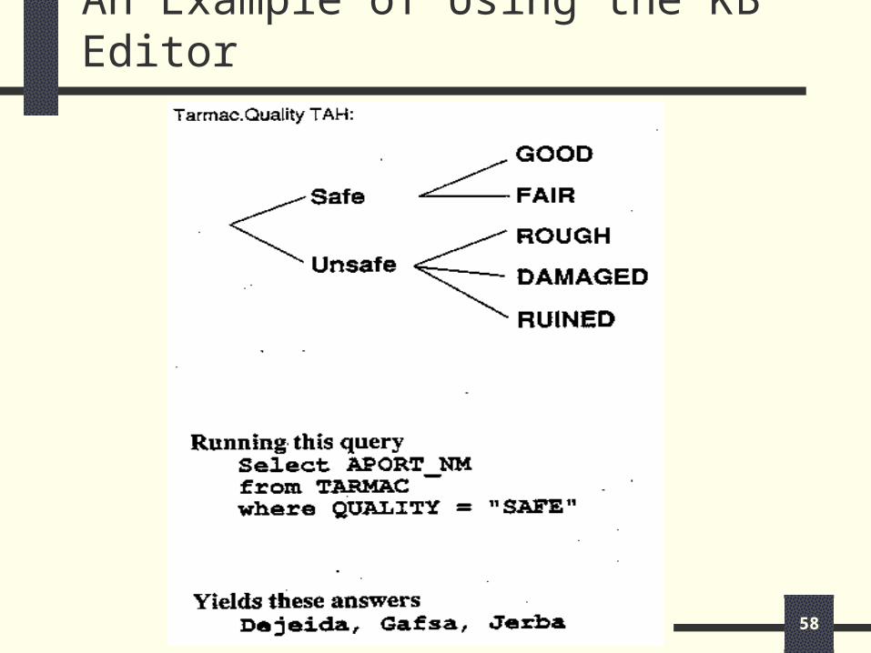
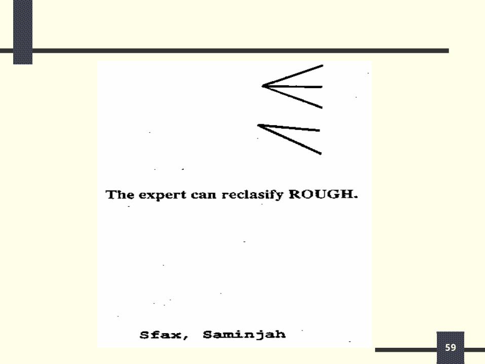
An Example of Using the KB Editor

59