data mining methods for malware detection

DATA MINING METHODS FOR MALWARE DETECTION

by

MUAZZAM AHMED SIDDIQUIB.E. NED University of Engineering and Technology, 1999

M.S. University of Central Florida, 2004

A dissertation submitted in partial fulfillment of the requirementsfor the degree of Doctor of Philosophy

in Modeling and Simulationin the College of Sciences

at the University of Central FloridaOrlando, Florida

Summer Term2008

Major Professor: Morgan C. Wang

c© 2008 Muazzam Ahmed Siddiqui

ii

ABSTRACT

This research investigates the use of data mining methods for malware (malicious programs) de-

tection and proposed a framework as an alternative to the traditional signature detection methods.

The traditional approaches using signatures to detect malicious programs fails for the new and un-

known malwares case, where signatures are not available. We present a data mining framework to

detect malicious programs. We collected, analyzed and processed several thousand malicious and

clean programs to find out the best features and build models that can classify a given program

into a malware or a clean class. Our research is closely related to information retrieval and classi-

fication techniques and borrows a number of ideas from the field. We used a vector space model

to represent the programs in our collection. Our data mining framework includes two separate

and distinct classes of experiments. The first are the supervised learning experiments that used a

dataset, consisting of several thousand malicious and clean program samples to train, validate and

test, an array of classifiers. In the second class of experiments, we proposed using sequential as-

sociation analysis for feature selection and automatic signature extraction. With our experiments,

we were able to achieve as high as 98.4% detection rate and as low as 1.9% false positive rate on

novel malwares.

iii

To Asma, without you, this journey would not have been possible.

To Erum, for always keeping faith in me.

To Ammi & Abbu, for all your prayers.

iv

TABLE OF CONTENTS

LIST OF FIGURES . . . . . . . . . . . . . . . . . . . . . . . . . . . . . . . . . . . . xvi

LIST OF TABLES . . . . . . . . . . . . . . . . . . . . . . . . . . . . . . . . . . . . . xviii

CHAPTER 1 INTRODUCTION . . . . . . . . . . . . . . . . . . . . . . . . . . . . 1

1.1 Definitions . . . . . . . . . . . . . . . . . . . . . . . . . . . . . . . . . . . . . . . 2

1.1.1 Computer Security . . . . . . . . . . . . . . . . . . . . . . . . . . . . . . 2

1.1.2 Malware . . . . . . . . . . . . . . . . . . . . . . . . . . . . . . . . . . . 2

1.1.3 Spam . . . . . . . . . . . . . . . . . . . . . . . . . . . . . . . . . . . . . 2

1.1.4 Phishing . . . . . . . . . . . . . . . . . . . . . . . . . . . . . . . . . . . 3

1.1.5 Exploits . . . . . . . . . . . . . . . . . . . . . . . . . . . . . . . . . . . . 3

1.2 Malware . . . . . . . . . . . . . . . . . . . . . . . . . . . . . . . . . . . . . . . . 3

1.2.1 Virus . . . . . . . . . . . . . . . . . . . . . . . . . . . . . . . . . . . . . 3

1.2.2 Worm . . . . . . . . . . . . . . . . . . . . . . . . . . . . . . . . . . . . . 4

1.2.3 Trojan . . . . . . . . . . . . . . . . . . . . . . . . . . . . . . . . . . . . . 4

1.2.4 Spyware . . . . . . . . . . . . . . . . . . . . . . . . . . . . . . . . . . . . 4

1.2.5 Others . . . . . . . . . . . . . . . . . . . . . . . . . . . . . . . . . . . . . 4

1.3 Virus . . . . . . . . . . . . . . . . . . . . . . . . . . . . . . . . . . . . . . . . . . 4

1.3.1 Classification by Target . . . . . . . . . . . . . . . . . . . . . . . . . . . . 5

1.3.1.1 Boot Sector Virus . . . . . . . . . . . . . . . . . . . . . . . . . 5

v

1.3.1.2 File Virus . . . . . . . . . . . . . . . . . . . . . . . . . . . . . 5

1.3.1.3 Macro Virus . . . . . . . . . . . . . . . . . . . . . . . . . . . . 5

1.3.2 Classification by Self-Protection Strategy . . . . . . . . . . . . . . . . . . 5

1.3.2.1 No Concealment . . . . . . . . . . . . . . . . . . . . . . . . . . 6

1.3.2.2 Code Obfuscation . . . . . . . . . . . . . . . . . . . . . . . . . 6

1.3.2.3 Encryption . . . . . . . . . . . . . . . . . . . . . . . . . . . . . 6

1.3.2.4 Polymorphism . . . . . . . . . . . . . . . . . . . . . . . . . . . 6

1.3.2.5 Metamorphism . . . . . . . . . . . . . . . . . . . . . . . . . . . 7

1.3.2.6 Stealth . . . . . . . . . . . . . . . . . . . . . . . . . . . . . . . 7

1.4 Worm . . . . . . . . . . . . . . . . . . . . . . . . . . . . . . . . . . . . . . . . . 7

1.4.1 Activation . . . . . . . . . . . . . . . . . . . . . . . . . . . . . . . . . . . 7

1.4.1.1 Human Activation . . . . . . . . . . . . . . . . . . . . . . . . . 8

1.4.1.2 Human Activity-Based Activation . . . . . . . . . . . . . . . . . 8

1.4.1.3 Scheduled Process Activation . . . . . . . . . . . . . . . . . . . 8

1.4.1.4 Self Activation . . . . . . . . . . . . . . . . . . . . . . . . . . . 8

1.4.2 Payload . . . . . . . . . . . . . . . . . . . . . . . . . . . . . . . . . . . . 8

1.4.2.1 None . . . . . . . . . . . . . . . . . . . . . . . . . . . . . . . . 8

1.4.2.2 Internet Remote Control . . . . . . . . . . . . . . . . . . . . . . 9

1.4.2.3 Spam-Relays . . . . . . . . . . . . . . . . . . . . . . . . . . . . 9

1.4.3 Target Discovery . . . . . . . . . . . . . . . . . . . . . . . . . . . . . . . 9

1.4.3.1 Scanning Worms . . . . . . . . . . . . . . . . . . . . . . . . . . 9

1.4.3.2 Flash Worms . . . . . . . . . . . . . . . . . . . . . . . . . . . . 9

vi

1.4.3.3 Metaserver Worms . . . . . . . . . . . . . . . . . . . . . . . . . 9

1.4.3.4 Topological Worms . . . . . . . . . . . . . . . . . . . . . . . . 10

1.4.3.5 Passive Worms . . . . . . . . . . . . . . . . . . . . . . . . . . . 10

1.4.4 Propagation . . . . . . . . . . . . . . . . . . . . . . . . . . . . . . . . . . 10

1.4.4.1 Self-Carried . . . . . . . . . . . . . . . . . . . . . . . . . . . . 10

1.4.4.2 Second Channel . . . . . . . . . . . . . . . . . . . . . . . . . . 10

1.4.4.3 Embedded . . . . . . . . . . . . . . . . . . . . . . . . . . . . . 10

1.5 Trojans . . . . . . . . . . . . . . . . . . . . . . . . . . . . . . . . . . . . . . . . 11

1.5.1 How Trojans Work . . . . . . . . . . . . . . . . . . . . . . . . . . . . . . 12

1.5.2 Trojan Types . . . . . . . . . . . . . . . . . . . . . . . . . . . . . . . . . 13

1.5.2.1 Remote Access Trojans . . . . . . . . . . . . . . . . . . . . . . 13

1.5.2.2 Password Sending Trojans . . . . . . . . . . . . . . . . . . . . . 13

1.5.2.3 Keyloggers . . . . . . . . . . . . . . . . . . . . . . . . . . . . . 13

1.5.2.4 Destructive . . . . . . . . . . . . . . . . . . . . . . . . . . . . . 14

1.5.2.5 Mail-Bomb Trojan . . . . . . . . . . . . . . . . . . . . . . . . . 14

1.5.2.6 Proxy/Wingate Trojans . . . . . . . . . . . . . . . . . . . . . . 14

1.5.2.7 FTP Trojans . . . . . . . . . . . . . . . . . . . . . . . . . . . . 15

1.5.2.8 Software Detection Killers . . . . . . . . . . . . . . . . . . . . 15

1.6 Data Mining . . . . . . . . . . . . . . . . . . . . . . . . . . . . . . . . . . . . . . 15

CHAPTER 2 LITERATURE REVIEW . . . . . . . . . . . . . . . . . . . . . . . . 17

2.1 Hierarchy . . . . . . . . . . . . . . . . . . . . . . . . . . . . . . . . . . . . . . . 18

vii

2.1.1 Detection Method . . . . . . . . . . . . . . . . . . . . . . . . . . . . . . . 18

2.1.1.1 Scanning . . . . . . . . . . . . . . . . . . . . . . . . . . . . . . 18

2.1.1.2 Activity Monitoring . . . . . . . . . . . . . . . . . . . . . . . . 19

2.1.1.3 Integrity Checking . . . . . . . . . . . . . . . . . . . . . . . . . 19

2.1.1.4 Data Mining . . . . . . . . . . . . . . . . . . . . . . . . . . . . 19

2.1.2 Feature Type . . . . . . . . . . . . . . . . . . . . . . . . . . . . . . . . . 19

2.1.2.1 N-grams . . . . . . . . . . . . . . . . . . . . . . . . . . . . . . 20

2.1.2.2 API/System calls . . . . . . . . . . . . . . . . . . . . . . . . . 20

2.1.2.3 Assembly Instructions . . . . . . . . . . . . . . . . . . . . . . . 20

2.1.2.4 Hybrid Features . . . . . . . . . . . . . . . . . . . . . . . . . . 20

2.1.2.5 Network Connection Records . . . . . . . . . . . . . . . . . . . 21

2.1.3 Analysis Type . . . . . . . . . . . . . . . . . . . . . . . . . . . . . . . . . 21

2.1.4 Detection Strategy . . . . . . . . . . . . . . . . . . . . . . . . . . . . . . 22

2.2 Scanners . . . . . . . . . . . . . . . . . . . . . . . . . . . . . . . . . . . . . . . . 23

2.2.1 Static Misuse Detection . . . . . . . . . . . . . . . . . . . . . . . . . . . 23

2.2.2 Hybrid Misuse Detection . . . . . . . . . . . . . . . . . . . . . . . . . . . 24

2.3 Activity Monitors . . . . . . . . . . . . . . . . . . . . . . . . . . . . . . . . . . . 24

2.3.1 API/System Calls . . . . . . . . . . . . . . . . . . . . . . . . . . . . . . . 24

2.3.1.1 Static Anomaly Detection . . . . . . . . . . . . . . . . . . . . . 24

2.3.1.2 Hybrid Anomaly Detection . . . . . . . . . . . . . . . . . . . . 25

2.3.1.3 Static Misuse Detection . . . . . . . . . . . . . . . . . . . . . . 25

2.3.1.4 Dynamic Anomaly Detection . . . . . . . . . . . . . . . . . . . 26

viii

2.3.1.5 Hybrid Misuse Detection . . . . . . . . . . . . . . . . . . . . . 27

2.3.1.6 Dynamic Misuse Detection . . . . . . . . . . . . . . . . . . . . 27

2.3.2 Hybrid Features . . . . . . . . . . . . . . . . . . . . . . . . . . . . . . . . 27



2.3.3 Network Data . . . . . . . . . . . . . . . . . . . . . . . . . . . . . . . . . 28


2.4 Integrity Checkers . . . . . . . . . . . . . . . . . . . . . . . . . . . . . . . . . . . 29

2.4.1 Static Anomaly Detection . . . . . . . . . . . . . . . . . . . . . . . . . . 29

2.5 Data Mining . . . . . . . . . . . . . . . . . . . . . . . . . . . . . . . . . . . . . . 30

2.5.1 N-grams . . . . . . . . . . . . . . . . . . . . . . . . . . . . . . . . . . . . 30


2.5.1.2 Dynamic Hybrid Detection . . . . . . . . . . . . . . . . . . . . 31


2.5.1.4 Static Hybrid Detection . . . . . . . . . . . . . . . . . . . . . . 32


2.5.2 API/System calls . . . . . . . . . . . . . . . . . . . . . . . . . . . . . . . 35



2.5.3 Assembly Instructions . . . . . . . . . . . . . . . . . . . . . . . . . . . . 37



ix

2.5.4 Hybrid Features . . . . . . . . . . . . . . . . . . . . . . . . . . . . . . . . 38



2.5.4.3 Hybrid Hybrid Detection . . . . . . . . . . . . . . . . . . . . . 40

CHAPTER 3 METHODOLOGY . . . . . . . . . . . . . . . . . . . . . . . . . . . . 41

3.1 Research Contribution . . . . . . . . . . . . . . . . . . . . . . . . . . . . . . . . 41

3.2 Learning Theory . . . . . . . . . . . . . . . . . . . . . . . . . . . . . . . . . . . 43

3.3 Vector Space Model . . . . . . . . . . . . . . . . . . . . . . . . . . . . . . . . . . 44

3.4 Models . . . . . . . . . . . . . . . . . . . . . . . . . . . . . . . . . . . . . . . . 46

3.4.1 Logistic Regression . . . . . . . . . . . . . . . . . . . . . . . . . . . . . . 46

3.4.2 Neural Network . . . . . . . . . . . . . . . . . . . . . . . . . . . . . . . . 46

3.4.3 Decision Tree . . . . . . . . . . . . . . . . . . . . . . . . . . . . . . . . . 47

3.4.4 Support Vector Machines . . . . . . . . . . . . . . . . . . . . . . . . . . . 47

3.4.5 Bagging . . . . . . . . . . . . . . . . . . . . . . . . . . . . . . . . . . . . 47

3.4.6 Random Forest . . . . . . . . . . . . . . . . . . . . . . . . . . . . . . . . 48

3.4.7 Principal Component Analysis . . . . . . . . . . . . . . . . . . . . . . . . 48

3.5 Performance Criteria . . . . . . . . . . . . . . . . . . . . . . . . . . . . . . . . . 48

CHAPTER 4 SUPERVISED LEARNING EXPERIMENTS . . . . . . . . . . . . . 50

4.1 Subset Data . . . . . . . . . . . . . . . . . . . . . . . . . . . . . . . . . . . . . . 52

4.1.1 Data Processing . . . . . . . . . . . . . . . . . . . . . . . . . . . . . . . . 52

4.1.1.1 Malware Analysis . . . . . . . . . . . . . . . . . . . . . . . . . 53

x

4.1.1.2 Disassembly . . . . . . . . . . . . . . . . . . . . . . . . . . . . 53

4.1.1.3 Parsing . . . . . . . . . . . . . . . . . . . . . . . . . . . . . . . 54

4.1.1.4 Feature Extraction . . . . . . . . . . . . . . . . . . . . . . . . . 54

4.1.1.5 Feature Selection . . . . . . . . . . . . . . . . . . . . . . . . . 56

4.1.1.6 Independence Test . . . . . . . . . . . . . . . . . . . . . . . . . 56

4.1.2 Experiments . . . . . . . . . . . . . . . . . . . . . . . . . . . . . . . . . 57

4.1.2.1 Logistic Regression . . . . . . . . . . . . . . . . . . . . . . . . 57

4.1.2.2 Neural Network . . . . . . . . . . . . . . . . . . . . . . . . . . 57

4.1.2.3 Decision Tree . . . . . . . . . . . . . . . . . . . . . . . . . . . 57

4.1.3 Results . . . . . . . . . . . . . . . . . . . . . . . . . . . . . . . . . . . . 58

4.2 Trojans . . . . . . . . . . . . . . . . . . . . . . . . . . . . . . . . . . . . . . . . 59

4.2.1 Data Processing . . . . . . . . . . . . . . . . . . . . . . . . . . . . . . . . 60


4.2.1.2 File Size Analysis . . . . . . . . . . . . . . . . . . . . . . . . . 61

4.2.1.3 Disassembly . . . . . . . . . . . . . . . . . . . . . . . . . . . . 62

4.2.1.4 Parsing . . . . . . . . . . . . . . . . . . . . . . . . . . . . . . . 62


4.2.1.6 Primary Feature Selection . . . . . . . . . . . . . . . . . . . . . 63


4.2.1.8 Secondary Feature Selection/Reduction . . . . . . . . . . . . . . 64

4.2.2 Experiments . . . . . . . . . . . . . . . . . . . . . . . . . . . . . . . . . 65

4.2.2.1 Bagging . . . . . . . . . . . . . . . . . . . . . . . . . . . . . . 65

xi

4.2.2.2 Random Forest . . . . . . . . . . . . . . . . . . . . . . . . . . . 65

4.2.2.3 Support Vector Machines . . . . . . . . . . . . . . . . . . . . . 65

4.2.3 Results . . . . . . . . . . . . . . . . . . . . . . . . . . . . . . . . . . . . 66

4.2.4 Discussion . . . . . . . . . . . . . . . . . . . . . . . . . . . . . . . . . . 66

4.3 Worms . . . . . . . . . . . . . . . . . . . . . . . . . . . . . . . . . . . . . . . . . 68

4.3.1 Data Processing . . . . . . . . . . . . . . . . . . . . . . . . . . . . . . . . 68


4.3.1.2 Disassembly . . . . . . . . . . . . . . . . . . . . . . . . . . . . 70


4.3.1.4 Feature Selection/Reduction . . . . . . . . . . . . . . . . . . . . 71


4.3.1.6 Feature Reduction . . . . . . . . . . . . . . . . . . . . . . . . . 72

4.3.1.7 Random Forest . . . . . . . . . . . . . . . . . . . . . . . . . . . 73

4.3.1.8 Principal Component Analysis . . . . . . . . . . . . . . . . . . 73

4.3.2 Experiments . . . . . . . . . . . . . . . . . . . . . . . . . . . . . . . . . 74

4.3.2.1 Bagging . . . . . . . . . . . . . . . . . . . . . . . . . . . . . . 74

4.3.2.2 Random Forest . . . . . . . . . . . . . . . . . . . . . . . . . . . 74

4.4 Results . . . . . . . . . . . . . . . . . . . . . . . . . . . . . . . . . . . . . . . . . 74

CHAPTER 5 UNSUPERVISED LEARNING EXPERIMENTS . . . . . . . . . . . 87

5.1 Feature Extraction . . . . . . . . . . . . . . . . . . . . . . . . . . . . . . . . . . . 88

5.1.1 Data Processing . . . . . . . . . . . . . . . . . . . . . . . . . . . . . . . . 88

xii

5.1.1.1 Data Partitioning . . . . . . . . . . . . . . . . . . . . . . . . . . 88

5.1.1.2 Data Transformation . . . . . . . . . . . . . . . . . . . . . . . . 89

5.1.2 Sequence Mining . . . . . . . . . . . . . . . . . . . . . . . . . . . . . . . 89

5.1.2.1 Feature Extraction Process . . . . . . . . . . . . . . . . . . . . 89

5.1.2.2 Dataset . . . . . . . . . . . . . . . . . . . . . . . . . . . . . . . 90


5.1.3 Experiments . . . . . . . . . . . . . . . . . . . . . . . . . . . . . . . . . 91

5.1.3.1 Random Forest . . . . . . . . . . . . . . . . . . . . . . . . . . . 91

5.1.4 Results . . . . . . . . . . . . . . . . . . . . . . . . . . . . . . . . . . . . 91

5.2 Automatic Malware Signature Extraction . . . . . . . . . . . . . . . . . . . . . . 92

5.2.1 Data Processing . . . . . . . . . . . . . . . . . . . . . . . . . . . . . . . . 93

5.2.1.1 Data Transformation . . . . . . . . . . . . . . . . . . . . . . . . 93

5.2.2 Signature Extraction . . . . . . . . . . . . . . . . . . . . . . . . . . . . . 94

5.2.2.1 Basic Algorithm . . . . . . . . . . . . . . . . . . . . . . . . . . 94

5.2.2.2 Modified Algorithm . . . . . . . . . . . . . . . . . . . . . . . . 96

5.2.3 Results . . . . . . . . . . . . . . . . . . . . . . . . . . . . . . . . . . . . 99

CHAPTER 6 CONCLUSIONS . . . . . . . . . . . . . . . . . . . . . . . . . . . . . 101

CHAPTER 7 FUTURE WORK . . . . . . . . . . . . . . . . . . . . . . . . . . . . . 102

7.1 Feature Extraction . . . . . . . . . . . . . . . . . . . . . . . . . . . . . . . . . . . 102

7.2 Signature Extraction . . . . . . . . . . . . . . . . . . . . . . . . . . . . . . . . . 103

7.3 PE Header . . . . . . . . . . . . . . . . . . . . . . . . . . . . . . . . . . . . . . . 103

xiii

7.4 Stratified Sampling . . . . . . . . . . . . . . . . . . . . . . . . . . . . . . . . . . 104

7.5 Real Time Implementation . . . . . . . . . . . . . . . . . . . . . . . . . . . . . . 104

7.5.1 Time and Space Complexity: . . . . . . . . . . . . . . . . . . . . . . . . . 104

7.5.2 Cost Sensitive Learning: . . . . . . . . . . . . . . . . . . . . . . . . . . . 104

7.5.3 Class Distribution: . . . . . . . . . . . . . . . . . . . . . . . . . . . . . . 105

7.6 Combining Classifiers . . . . . . . . . . . . . . . . . . . . . . . . . . . . . . . . . 105

7.7 More Classifiers . . . . . . . . . . . . . . . . . . . . . . . . . . . . . . . . . . . . 105

LIST OF REFERENCES . . . . . . . . . . . . . . . . . . . . . . . . . . . . . . . . . 106

xiv

LIST OF FIGURES

4.1 Typical 32-Bit Portable .EXE File Layout . . . . . . . . . . . . . . . . . . . . . . 51

4.2 Portion of the output of disassembled actmovie.exe. . . . . . . . . . . . . . . . . . 53

4.3 Instruction sequences extracted from actmovie.exe . . . . . . . . . . . . . . . . . 54

4.4 Scatter plot of sequence frequencies and their frequency of occurrence. . . . . . . . 55

4.5 Scatter plot of sequence frequencies and their frequency of occurrence with outliers

removed. . . . . . . . . . . . . . . . . . . . . . . . . . . . . . . . . . . . . . . . 55

4.6 Data preprocessing steps for experiments with the malware subset. . . . . . . . . . 56

4.7 ROC curve comparing regression, neural network and decision tree training results. 58

4.8 ROC curve comparing regression, neural network and decision tree test results. . . 59

4.9 2007 Malware distribution statistics from Trend Micro. . . . . . . . . . . . . . . . 60

4.10 Portion of the output of disassembled Win32.Flood.A trojan. . . . . . . . . . . . . 63

4.11 Instruction sequences extracted from the disassembled Win32.Flood.A trojan. . . . 63

4.12 Data preprocessing steps for experiments with trojans. . . . . . . . . . . . . . . . 64

4.13 ROC curve comparing random forest test results on datasets with all variables, RF

variables and PCA variables. . . . . . . . . . . . . . . . . . . . . . . . . . . . . . 66

4.14 ROC curve comparing random forest, bagging and SVM test results on dataset

with RF selection. . . . . . . . . . . . . . . . . . . . . . . . . . . . . . . . . . . . 67

4.15 Portion of the output of disassembled Netsky.A worm. . . . . . . . . . . . . . . . 70

4.16 Instruction sequences extracted from the disassembled Netsky.A worm. . . . . . . 71

4.17 Data preprocessing steps for experiments with worms. . . . . . . . . . . . . . . . 71

xv

4.18 ROC curves comparing random forest results for each n-gram size using all variables. 79

4.19 ROC curves comparing random forest results for each n-gram size using random

forest feature selection. . . . . . . . . . . . . . . . . . . . . . . . . . . . . . . . . 80

4.20 ROC curves comparing random forest results for each n-gram size using PCA fea-

ture reduction. . . . . . . . . . . . . . . . . . . . . . . . . . . . . . . . . . . . . . 80

4.21 ROC curves comparing bagging results for each n-gram size using all variables. . . 81

4.22 ROC curves comparing bagging results for each n-gram size using random forest

feature selection. . . . . . . . . . . . . . . . . . . . . . . . . . . . . . . . . . . . 81

4.23 ROC curves comparing bagging results for each n-gram size using PCA feature

reduction. . . . . . . . . . . . . . . . . . . . . . . . . . . . . . . . . . . . . . . . 82

4.24 ROC curves comparing random forest and bagging results using random forest

feature selection. . . . . . . . . . . . . . . . . . . . . . . . . . . . . . . . . . . . 82

4.25 ROC curves comparing the variable selection methods (all variables, RF variables,

PCA variables) . . . . . . . . . . . . . . . . . . . . . . . . . . . . . . . . . . . . 83

5.1 ROC curves comparing the results for the features selected using sequence associ-

ation mining only and the combined feature set. . . . . . . . . . . . . . . . . . . . 92

xvi

LIST OF TABLES

4.1 Experimental results for new and unknown viruses. . . . . . . . . . . . . . . . . . 59

4.2 Area under the ROC curve for each classifier. . . . . . . . . . . . . . . . . . . . . 60

4.3 Packers/Compilers Analysis of Trojans . . . . . . . . . . . . . . . . . . . . . . . . 61

4.4 Packers/Compilers Analysis of Trojans and Clean Programs . . . . . . . . . . . . 61

4.5 File Size Analysis of the Program Collection . . . . . . . . . . . . . . . . . . . . . 62

4.6 Experimental results for new and unknown trojans. . . . . . . . . . . . . . . . . . 66

4.7 Area under the ROC curve for each classifier for each dataset. . . . . . . . . . . . 67

4.8 Packers/Compilers Analysis Details of Worms and Clean Programs . . . . . . . . . 69

4.9 Packers/Compilers Analysis Summary of Worms and Clean Programs . . . . . . . 69

4.10 Features Statistics . . . . . . . . . . . . . . . . . . . . . . . . . . . . . . . . . . . 72

4.11 Reduced Feature Sets . . . . . . . . . . . . . . . . . . . . . . . . . . . . . . . . . 73

4.12 Experimental results for new and unknown worms. . . . . . . . . . . . . . . . . . 75

4.13 Area under the ROC curve for each classifier. . . . . . . . . . . . . . . . . . . . . 83

5.1 Experimental results for new and unknown malwares using sequential association

analysis as well as a combined selection method. . . . . . . . . . . . . . . . . . . 91

5.2 Truth table for the basic algorithm. . . . . . . . . . . . . . . . . . . . . . . . . . . 95

5.3 Truth table for the modified algorithm for clean files. . . . . . . . . . . . . . . . . 97

5.4 Truth table for the modified algorithm for malwares. . . . . . . . . . . . . . . . . . 98

5.5 Truth table for the modified algorithm for malwares and clean programs . . . . . . 98

xvii

5.6 Experimental results for new and unknown malwares using automatically extracted

signatures by applying sequential association mining. . . . . . . . . . . . . . . . . 100

xviii

CHAPTER 1INTRODUCTION

Computer virus detection has evolved into malicious program detection since Cohen first formal-

ized the term computer virus in 1983 [Coh85]. Malicious programs can be classified into viruses,

worms, trojans, spywares, adwares and a variety of other classes and subclasses that sometimes

overlap and blur the boundaries among these classes [Szo05]. Both traditional signature based

detection and generalized approaches can be used to identify these malicious programs. To avoid

detection by the traditional signature-based algorithms, a number of stealth techniques have been

developed by the malicious code writers. The inability of traditional signature based detection

approaches to catch these new breed of malicious programs has shifted the focus of virus research

to find more generalized and scalable features that can identify malicious behavior as a process

instead of a single signature action.

We present a data mining approach to the problem of malware detection. Data mining has

been a recent focus of malware detection research. Section 2.5 presents a literature review of the

data mining techniques used for virus and worm detection. Our approach combines the ease of an

automated syntactic analysis with the power of semantic level analysis requiring human expertise

to reflect critical program behavior that can classify between malicious and benign programs. We

performed initial experiments and developed a data mining framework that serves as a platform for

further research.

1

1.1 Definitions

This section introduces various computer security terms to the reader. Since our work deals with

computer virus and worms, a more detailed account of these categories is presented than any other

area in security.

1.1.1 Computer Security

Computer security is the effort to create a secure computing platform, designed so that agents

(users or programs) can only perform actions that have been allowed.

1.1.2 Malware

Any program that is purposefully created to harm the computer system operations or data is termed

as malicious programs. Malicious programs include viruses, worms, trojans, backdoors, adwares,

spywares, bots, rootkits etc. All malwares are sometimes loosely termed as virus (viruses, worms,

trojans specifically) Commercial anti-malware products are still called antivirus.

1.1.3 Spam

Spam is abuse of electronic messaging systems to send unsolicited bulk messages Most widely

recognized form is email spam. Also includes IM spam, blog spam, discussion forum spam, cell

phone messaging spam etc.

2

1.1.4 Phishing

Phishing can be defined as a criminal activity using social engineering techniques. The most

common example of phishing is an email asking to enter account/credit card information for e-

commerce websites (ebay, amazon etc) and online banking.

1.1.5 Exploits

An exploit is a piece of software, a chunk of data, or sequence of commands that take advantage

of a bug, glitch or vulnerability in order to cause unintended or unanticipated behavior to occur

on computer software, hardware, or something electronic (usually computerized). This frequently

includes such things as gaining control of a computer system or allowing privilege escalation or a

denial of service attack.

1.2 Malware

Malware is a relatively new term that gets its name from malicious software. Many users are still

unfamiliar with the term. Most of the time all malware are grouped under the umbrella term virus.

For the detection of malware, the industry still use the term antivirus not antimalware, though the

product caters all malware.

1.2.1 Virus

Computer virus is a self replicating code (including possibly evolved copies of itself) that infects

other executable programs. Viruses usually need human intervention for replication and execution.

3

1.2.2 Worm

Computer worm is a self replicating stand alone program that spreads on computer networks.

Worms usually do not need any extra help from a user to replicate and execute.

1.2.3 Trojan

Trojan horses or simply trojans are programs that perform some malicious activity under the guise

of some normal program. The term is derived from the classical myth of the Trojan Horse.

1.2.4 Spyware

Spyware is computer software that is installed surreptitiously on a personal computer to intercept

or take partial control over the user’s interaction with the computer, without the user’s informed

consent.

1.2.5 Others

Other malware programs include logic bombs, that are an intended malfunction of a legitimate

program, rootkits, that are a set of hacker tools intended to conceal running process from operating

system, backdoor, that is a method to bypass normal computer authentication.

1.3 Virus

Computer virus is a self replicating code (including possibly evolved copies of itself) that infects

other executable programs. Viruses usually need human intervention for replication and execution.

4

1.3.1 Classification by Target

This section define target as the means exploited by the virus for execution. Based upon the target

viruses can be classified into three major classes.

1.3.1.1 Boot Sector Virus

Master Boot Record (Boot sector in DOS) is a piece of code that runs every time a computer

system is booted. Boot sector virus infect the MBR on the disk, hence getting the privilege of

getting executed every time the computer system starts up.

1.3.1.2 File Virus

File virus is the most common form of viruses. They infect the file system on a computer. File

virus infect executable programs and are executed every time the infected program is run.

1.3.1.3 Macro Virus

Macro virus infect documents and templates instead of executable programs. It is written in a

macro programming language that is built into applications like Microsoft Word or Excel. Macro

virus can be automatically executed every time the document is opened with the application.

1.3.2 Classification by Self-Protection Strategy

Self-protection strategy can be defined as the technique used by a virus to avoid detection. In

other words, the anti-antivirus techniques. Based upon self-protection strategies, viruses can be

classified into the following categories.

5

1.3.2.1 No Concealment

Based upon the self-protection strategy the first category can be defined as the one without any

concealment. The virus code is clean without any garbage instructions or encryption.

1.3.2.2 Code Obfuscation

Code obfuscation is a technique developed to avoid specific-signature detection. These include

adding no-op instructions, unnecessary jumps etc, so the virus code look muddled and the signature

fails.

1.3.2.3 Encryption

The next line of defense by the virus writers to defeat signature detection was code encryption.

Encrypted viruses use an encrypted virus body and an unencrypted decryption engine. For each

infection, the virus is encrypted with a different key to avoid giving a constant signature.

1.3.2.4 Polymorphism

Encrypted virus were caught by the presence of the unencrypted decryption engine that remain

constant for every infection. This was cured by the mutating techniques. Polymorphic virus feature

a mutation engine that generates the decryption engine on the fly. It consists of a decryption engine,

a mutation engine and payload. The encrypted virus body and the mutating decryption engine

refused to provide a constant signature.

6

1.3.2.5 Metamorphism

Metamorphic virus is a self mutating virus in its truest form of the word at it has no constant parts.

The virus body itself changes during the infection process and hence the infected file represents a

new generation that does not resemble the parent.

1.3.2.6 Stealth

Stealth techniques, also called code armoring, refers to the set of techniques developed by the

virus writers to avoid the recent detection methods of activity monitoring, code emulation etc. The

techniques include anti-disassembly, anti-debugging, anti-emulation, anti-heuristics etc.

1.4 Worm

A computer worm is a program that self-propagates across a network exploiting security or policy

flaws in widely-used services.

Dan Ellis [Ell03], defined the life cycle of worms. Based upon the operations involved in each

phase in the life cycle, worms can be classified into different categories. The following taxonomy

was used by [WPS03] using similar factors.

1.4.1 Activation

Activation defines the means by which a worm is activated onto the target system. This is the first

phase in a worms life cycle. Based upon activation techniques worms can be classified into the

following classes.

7

1.4.1.1 Human Activation

This is the slowest form of activation that requires a human to execute the worm.

1.4.1.2 Human Activity-Based Activation

In this form of activation, the worm execution is based upon some action that the user perform not

directly related to the worm such as launching an application program etc.

1.4.1.3 Scheduled Process Activation

This type of activation depends upon scheduled system processes such as automatic download of

software updates etc.

1.4.1.4 Self Activation

This is the fastest form of activation where a worm initialize its execution by exploiting the vul-

nerabilities in the programs that are always running such as database or web servers.

1.4.2 Payload

The next phase in the worm’s life cycle is payload delivery. Payload describes what a worm does

after the infection.

1.4.2.1 None

Majority of worms do not carry any payload. The still cause havoc by increasing machine and

network traffic load.

8

1.4.2.2 Internet Remote Control

Some worms open a backdoor on the victims machine thus allowing others to connect to that

machine via internet.

1.4.2.3 Spam-Relays

Some worms convert the victim machine into a spam relay, thus allowing spammers to use it as a

server.

1.4.3 Target Discovery

Once the payload is delivered, the worm start looking for new targets to attack.

1.4.3.1 Scanning Worms

Scanning worms scan for targets by scanning sequentially through a block of addresses or by

scanning randomly.

1.4.3.2 Flash Worms

Flash worms use a pre-generated target list or a hit list to accelerate the target discovery process.

1.4.3.3 Metaserver Worms

This type of worms use a list of addresses to infect maintained by an external metaserver.

9

1.4.3.4 Topological Worms

Topological worms try to find the local communication topology by searching through a list of

hosts maintained by application programs.

1.4.3.5 Passive Worms

Passive worms rely on user intervention or targets to contact worm for their execution.

1.4.4 Propagation

Propagation defines the means by which a worm spreads on a network. Based upon the propagation

mechanism worms can be divided into the following categories.

1.4.4.1 Self-Carried

Self carried worms are usually self activated. They copy themselves to the target as part of the

infection process.

1.4.4.2 Second Channel

Second channel worm copy their body after the infection by creating a connection from target to

host to download the body.

1.4.4.3 Embedded

Embedded worms, embed themselves in the normal communication process as a stealth technique.

10

1.5 Trojans

While the words Trojan, worm and virus are often used interchangeably, they are not the same.

Viruses, worms and Trojan Horses are all malicious programs that can cause damage to your

computer, but there are differences among the three. A Trojan horse, also known as a Trojan, is a

piece of malware, which appears to perform a certain action but in fact performs another such as

transmitting a computer virus. At first glance it will appear to be useful software but will actually

do damage once installed or run on your computer. Those on the receiving end of a Trojan horse

are usually tricked into opening them because they appear to be receiving legitimate software

or files from a legitimate source. When a Trojan is activated on your computer, the results can

vary. Some Trojans are designed to be more annoying than malicious (like changing your desktop,

adding silly active desktop icons) or they can cause serious damage by deleting files and destroying

information on your system. Trojans are also known to create a backdoor on your computer that

gives malicious users access to your system, possibly allowing confidential or personal information

to be compromised. Unlike viruses and worms, Trojans do not reproduce by infecting other files

nor do they self-replicate. Simply put, a Trojan horse is not a computer virus. Unlike such malware,

it does not propagate by self-replication but relies heavily on the exploitation of an end-user. It is

instead a categorical attribute, which can encompass many different forms of codes. Therefore, a

computer worm or virus may be a Trojan horse. The term is derived from the classical story of the

Trojan horse.

11

1.5.1 How Trojans Work

Trojans usually consist of two parts, a Client and a Server. The server is run on the victim’s

machine and listens for connections from a Client, which is used by the attacker. When the server

is run on a machine it will listen on a specific port or multiple ports for connections from a Client.

In order for an attacker to connect to the server they must have the IP Address of the computer

where the server is being run. Some Trojans have the IP Address of the computer they are running

on sent to the attacker via email or another form or communication. Once a connection is made

to the server, the client can then send commands to the server; the server will then execute these

commands on the victim’s machine.

Today, with NAT infrastructure being very common, most computers cannot be reached by their

external IP address. Therefore many Trojans now connect to the computer of the attacker, which

has been set up to take the connections, instead of the attacker connecting to his or her victim. This

is called a ’reverse-connect’ Trojan. Many Trojans nowadays also bypass many personal firewall

installed on the victims computer. (E.g. Poison Ivy)

Trojans are extremely simple to create in many programming languages. A simple Trojan in

Visual Basic or C# using Visual Studio can be achieved in 10 lines of code or under. Probably

the most famous Trojan horse is the AIDS TROJAN DISK that was sent to about 7000 research

organizations on a diskette. When the Trojan was introduced on the system, it scrambled the name

of all files (except a few) and filled the empty areas of the disk completely. The program offered a

recovery solution in exchange of a bounty. Thus, malicious cryptography was born.

12

1.5.2 Trojan Types

Trojans are generally the programs that pose as legitimate programs on your computer and add a

subversive functionality to it. That’s when it’s said a program is Trojaned. Common functions of

Trojans include, but are not limited to, the following:

1.5.2.1 Remote Access Trojans

These are probably the most widely used trojans, just because they give the attackers the power to

do more things on the victim’s machine than the victim itself while being in front of the machine.

Most of these trojans are often a combination of the other variations described below. The idea

of these trojans is to give the attacker a total access to someone’s machine and therefore access to

files, private conversations, accounting data, etc.

1.5.2.2 Password Sending Trojans

The purpose of these trojans is to rip all the cached passwords and also look for other passwords

you’re entering and then send them to a specific mail address without the user noticing anything.

Passwords for ICQ, IRC, FTP, HTTP or any other application that require a user to enter a lo-

gin+password are being sent back to the attacker’s email address, which in most cases is located

at some free web based email provider.

1.5.2.3 Keyloggers

These trojans are very simple. The only thing they do is logging the keystrokes of the victim and

then letting the attacker search for passwords or other sensitive data in the log file. Most of them

13

come with two functions like online and offline recording. Of course, they could be configured to

send the log file to a specific email address on a schedule basis.

1.5.2.4 Destructive

The only function of these trojans is to destroy and delete files. This makes them very simple

and easy to use. They can automatically delete all the system files on your machine. The trojan

is being activated by the attacker or sometimes works like a logic bomb and starts on a specific

day and at specific hour. Denial Of Service (DoS) Attack Trojans These trojans are getting very

popular these days, giving the attacker the power to start DDoS when having enough victims, of

course. The main idea is that if you have 200 ADSL users infected and start attacking the victim

simultaneously, this will generate a lot of traffic (more then the victim’s bandwidth, in most cases)

and its the access to the Internet will be shut down.

1.5.2.5 Mail-Bomb Trojan

This is another variation of a DoS trojan whose main aim is to infect as many machines as possi-

ble and simultaneously attack specific email address/addresses with random subjects and contents

which cannot be filtered.

1.5.2.6 Proxy/Wingate Trojans

The interesting feature implemented in many trojans is turning the victim’s computer into a proxy/wingate

server available to the whole world or to the attacker only. It’s used for anonymous Telnet, ICQ,

IRC, etc., and also for registering domains with stolen credit cards and for many other illegal ac-

14

tivities. This gives the attacker complete anonymity and the chance to do everything from your

computer, and if he/she gets caught, the trace leads back to you.

1.5.2.7 FTP Trojans

These trojans are probably the most simple ones and are kind of outdated as the only thing they do

is to open port 21 (the port for FTP transfers) and let everyone or just the attacker connect to your

machine. Newer versions are password protected, so only the one who infected you may connect

to your computer.

1.5.2.8 Software Detection Killers

There are such functionalities built into some trojans, but there are also separate programs that

will kill ZoneAlarm, Norton Anti-Virus and many other (popular anti-virus/firewall) programs that

protect your machine. When they are disabled, the attacker will have full access to your machine

to perform some illegal activity, use your computer to attack others and often disappear. Even

though you may notice that these programs are not working or functioning properly, it will take

you some time to remove the trojan, install the new software, configure it and get back online with

some sense of security.

1.6 Data Mining

Data mining has been defined as ”the nontrivial extraction of implicit, previously unknown, and

potentially useful information from data” [FPM92] and ”the science of extracting useful informa-

tion from large data sets or databases” [HH01].

15

Data mining can be divided into two broad categories.

• Predictive data mining, involves predicting unknown values based upon given data items.

• Descriptive data mining, involves finding patterns describing the data.

[Kan02] described the following tasks associated with data mining.

• Classification: the process of classifying data items into two or more pre defined classes.

• Regression: predicting the average value of one item on the basis of known value(s) of other

item(s).

• Clustering: identifying a finite set of categories for the data.

• Summarization: finding a compact description of the data.

• Dependency Modeling: finding a local model that describes significant dependencies be-

tween variables.

• Change and Deviation Detection: discovering the most significant changes in the data set.

The final outcome of a data mining process is a model or a collection of models. A number

of data mining techniques are available for the model building process. These techniques are not

limited to the this final stage though. Any previous data mining stage e.g. data preprocessing may

use these techniques.

16

CHAPTER 2LITERATURE REVIEW

Chapter 1 provided a brief overview of the areas in computer security with special emphasis on

viruses and worms. In this chapter, a literature survey is provided that structures the theoretical

foundation for this research.

The term computer virus was first used in a science fiction novel by David Gerrold in 1972,

When HARLIE Was One [Ger72], which includes a description of a fictional computer program

called virus and was able to self-replicate. The first academic use of the term was claimed by

Fred Cohen in 1983. The first published account of the term can be found a year later by Cohen

in his paper Experiments with Computer Viruses [Coh84]. In his paper Cohen credits his advisor

Professor Len Adleman for coining the term.

Though Cohen first used the term, some early accounts of viruses can be found. According to

[Fer92], the first reported incidents of true viruses were in 1981 and 1982 on the Apple II computer.

Elk Cloner is considered to be the first documented example of a virus in mid-1981. The first PC

virus was a boot sector virus called Brain in 1986 [JH90].

Worm also owe their existence to science fiction literature. John Brunner’s Shockwave Rider

[Bru75] introduced us to worm, a program that propagates itself on a computer network. [SH82]

claim the first use of the term in academic circles.

Much has been written about viruses, worms, trojans and other malwares since then, but now

we shift our focus, from fiction to the real world where both malware and anti-malware are big

commercial industries now [Gut07]. As this work is related to malware detection, this chapter

provides a literature survey of the area.

17

2.1 Hierarchy

We applied a hierarchical approach to organize the research into a four tier categorization. The

actual detection method sits at the top level of the hierarchy, followed by feature type, analysis

type and detection strategy. This work categorizes the malware detection methods into four broad

categories; scanning, activity monitoring, integrity checking and data mining. File features are the

features extracted from binary programs, analysis type is either static or dynamic, and the detection

type is borrowed from intrusion detection as either misuse or anomaly detection. It provides the

reader with the major advancement in the malware research and categorizes the surveyed work

based upon the above stated hierarchy, which served as the one of the contributions of this research.

2.1.1 Detection Method

The first three categories have been mentioned in previous works, [Spa94], [Bon96]. We have

added data mining as a fourth category. We define the detection mechanism as a two stage process:

data collection and the core detection method. The above defined categories compete for the,

second, core detection part. Otherwise, it is possible that activity monitoring is employed to collect

data and extract features which are later used, either to train a classifier or as signatures in a scanner,

after further processing. Based upon this criteria, we define the four categories as follows:

2.1.1.1 Scanning

Scanning is the most widely used industry standard. Scanning involve searching for strings in files.

The strings being searched are pre-defined virus signatures and support exact matching as well as

wildcards to look for variants of a virus.

18

2.1.1.2 Activity Monitoring

Activity Monitoring is the latest trend in virus research where a file execution is monitored for

traces of malicious behavior.

2.1.1.3 Integrity Checking

Integrity Checking creates a cryptographic checksum for each file on a system and periodically

monitors for any variation in that checksum to detect possible changes caused by viruses.

2.1.1.4 Data Mining

Data Mining involves the application of a full suite of statistical and machine learning algorithms

on a set of features derived from malicious and clean programs.

2.1.2 Feature Type

Feature type describes the input data to the malware detection system. The source of this data

serves as a classification criteria for many intrusion and malware detection systems. If the data

source is a workstation, the detection is called Host-Based Detection. If the source is the network,

the detection is termed as Network-Based Detection. Features extracted from programs are used

in a host based detection system. Various reverse engineering techniques at different stages are

applied to extract byte sequences, instruction sequences, API call sequences etc. Network-based

detection systems use network connection records as their data source.

19

2.1.2.1 N-grams

An N-gram is a sequence of bytes of fixed or variable length, extracted form the hexadecimal dump

of an executable program. Here, we are using n-grams as a general term for both overlapping and

non-overlapping byte sequences. For the sake of this paper, we define n-grams to remain at a

syntactic level of analysis.

2.1.2.2 API/System calls

An application programming interface (API) is a source code interface that an operating system or

library provides to support requests for services to be made of it by computer programs [api]. For

operating system requests, API is interchangeably termed as system calls. An API call sequences

captures the activity of a program and, hence, is an excellent candidate for mining of any malicious

behavior.

2.1.2.3 Assembly Instructions

In more recent developments, it was emphasized that since n-grams fail to capture the semantics

of the program, instruction sequences should be used instead. Unlike extracting n-grams from

hexdumps, instructions need disassembling the binaries. We define, assembly instruction features

to be instructions of variable and/or fixed lengths extracted from disassembled files.

2.1.2.4 Hybrid Features

A number of techniques used a collection of features, either for different classifiers, or as a hybrid

feature set for the same classifier. The work done by [SEZ01b] used three different features includ-

20

ing n-grams, DLL usage information and strings extracted from the binaries. Since this work was

made famous for its usage of n-grams, we finally decided to place it in the n-grams section.

2.1.2.5 Network Connection Records

A network connection record is a set of information, such as duration, protocol type, number of

transmitted bytes etc, which represents a sequence of data flow to and from a well defined source

and target.

2.1.3 Analysis Type

The analysis can be performed at the source code level or at the binary level where only the exe-

cutable program is available. As mentioned by [BDD99], it is unrealistic to assume the availability

of source code for every program. The only choice left are executables with certain legal bindings.

The information from the executables can be gathered either by running them or performing static

reverse engineering or by using both techniques. The reverse engineering method is called Static

Analysis while the process in which the program is actually executed to gather the information is

called Dynamic Analysis. A mixed approach is also utilized if needed.

Static analysis offers information about programs control and data flow and other statistical

features without actually running the program. Several reverse engineering methods are applied

to create an intermediate representation of the binary code. These include disassembling, decom-

piling etc. Once the data is in human readable format, other techniques can be applied for further

analysis. The major advantage of static analysis over its dynamic counterpart is that its free from

the overhead of execution time. The major drawback lies inherently in any static reverse engi-

21

neering method being an approximation of the actual execution. At any decision point, it is only

guessed which branch will be taken at the execution time, though the guess is often accurate.

Dynamic analysis require running the program and monitoring its execution in a real or a virtual

machine environment. Though this gives the actual information about the control and data flow,

this approach severely suffers from the execution overhead. A mixed analysis approach is often

used that run portions of the code when static analysis fails to make a proper decision [Sym97].

2.1.4 Detection Strategy

All of these methods involve a matching/mismatching criteria to work. Based upon this criteria the

method can be classified as an anomaly detection, a misuse detection or a hybrid detection method.

Anomaly Detection involves creating a normal profile of the system or programs and checking for

any deviation from that profile. Misuse Detection involves creating a malicious profile in the

form of an exact or heuristic signature and checking for that signature in the programs. Hybrid

Detection does not create any profile but uses data from both clean and malicious programs to

build classifiers. An anomaly detection system looks for mismatches from normal profile, while a

misuse detection system looks for matches for virus signatures.

[SL02] presented an excellent survey of virus and worm research where they cited important

work in virus and worm theory, modeling, analysis and detection. [IM07] offers a taxonomy with

their survey of malware detection research. Besides the hierarchical structure, the classification

presented in this dissertation differs from [IM07] at two points.

• It includes literature describing theory, modeling and analysis besides detection.

• The definition used for dynamic and static analysis is different as [IM07] classified between

22

the two approaches based upon the data they are operating on. If it is execution data e.g.

system calls, instructions etc. then the analysis is termed as dynamic whereas static analysis

operates on non execution items e.g. frequencies.

The following sections review virus and worm research literature using the criteria defined

above.

2.2 Scanners

Scanners are the necessary component of every commercial-off-the-shelf (COTS) antivirus pro-

gram. As [Szo05] indicated, the scanners have matured from simple string scanning to heuristic

scanning. Nevertheless the concept remains the same. Searching for signatures in the target file.

2.2.1 Static Misuse Detection

Scanning or file scanning as it sometimes referred to, is essentially a static misuse detection tech-

nique. [Szo05] reviewed a number of scanning techniques in his book including string scanning,

that is simply exact string searching, wildcard scanning, that allows for wildcards to cover variants

(signatures with slight modification), smart scanning, that discards garbage instructions to thwart

simple mutations, nearly exact identification, that accompany the primary virus signature with a

secondary one to detect variants, exact identification, that uses as many secondary signatures as

required to detect all the variants in a virus family and heuristic scanning, that scans for malicious

behavior in the form of a series of actions.

As [Bon96] pointed out with the advent of polymorphic viruses, the virus-specific scanners

have exhausted themselves, [Gry99] argued that the new wave in virus detection research will be

23

heuristic scanners.

2.2.2 Hybrid Misuse Detection

[Sym97] used the mixed approach in their Bloodhound technology where they supplement static

analysis with code emulation in their heuristic scanner. The scanner isolate logical region of the

target program and analyze the logic for each region for a virus like behavior.

Symantec’s Striker technology [Sym96] also used code emulation and heuristic scanning to

detect polymorphic viruses. Virus profiles were created for each polymorphic engine and mutation

engine that were based upon behavioral signatures.

2.3 Activity Monitors

Activity monitors use both static and dynamic analysis. Though the term static activity monitoring

carry some sense of being an oxymoron, nevertheless, static analysis make it possible to monitor

the execution of a program without actually running it.

2.3.1 API/System Calls

The most common method to monitor the activity of a program is to monitor the API/system calls

it is making.

2.3.1.1 Static Anomaly Detection

[WD01] proposed a technique that created a control flow graph for a program representing its

system call trace. At execution time this CFG was compared with the system call sequences to

24

check for any violation.

2.3.1.2 Hybrid Anomaly Detection

[RKL03] proposed an anomaly based technique where static analysis was assisted by dynamic

analysis to detect injected, dynamically generated and obfuscated code. The static analysis was

used to identify the location of system calls within the program. The programs can be dynamically

monitored later to verify that each observed system call is made from the same location identified

using the static analysis.

2.3.1.3 Static Misuse Detection

[BDE99] used a static misuse detection scheme where they used program slicing to extract program

regions that are critical from a security point of view. Prior to this, the programs were disassem-

bled and converted to an intermediate representation. Once the program slices are obtained, their

behavior was checked against a pre-defined security policy to detect the presence of maliciousness.

In a related work [BDD01] extracted an API call graph instead of the program slices to test

against the security policy. The programs were disassembled first and then an control graph is

created from the disassembly. Next step was to extract the API call graph from the control graph.

[LLO95] proposed the idea of tell-tale signs which were heuristic signatures of malicious pro-

gram behaviors. They created an intermediate representation of the program under investigation

in the form of control flow graph. The CFG was verified against the tell-tale signs to detect any

malicious activity. The approach was implemented in their system called Malicious Code Filter

(MCF).

25

[SXC04] implemented signatures in the form of API calls in a technique called Static Anal-

ysis for Vicious Executables (SAVE). The API calls from any program under investigation were

compared against the signature calls using Euclidean distance.

2.3.1.4 Dynamic Anomaly Detection

[HFS98] proposed anomaly detection based upon sequence of system calls. A normal profile

was composed of short sequence of system calls. Hamming distance was used to compare the

sequences of system calls. Large Hamming distances indicated longer sequences and were thus

marked as anomalous.

In a similar approach [SBB01] used Finite State Automata (FSA) to represent system call

sequences. The FSAs were created by executing the programs multiple times and recording the

system calls. Anomalies were detected at runtime when a system call is made that did not have a

transition from a given FSA state.

Similarly [KRL97] proposed an idea of trace policy which was essentially a sequence of system

calls in time. Any deviation from this trace policy was flagged as anomaly. They implemented this

approach in a system called Distributed Program Execution Monitor (DPEM).

[MP05] presented a tool called Dynamic Information Flow Analysis (DIFA) to monitor method

calls at runtime for Java applications. Normal behavior was implemented in the form of an infor-

mation flow policy. Deviations from this policy at runtime were marked as anomalies.

[SB99] created a system call detection engine that compares system calls modeled previously

with the system calls made at runtime. An intermediate representation of a program was captured

in the form of an Auditing Specification Language (ASL). The ASL was compiled into a C++ class

26

that was then compiled and linked to create a model of a system call in the system call detection

engine.

2.3.1.5 Hybrid Misuse Detection

[Mor04] presented an approach to detect encrypted and polymorphic viruses using static analysis

and code emulation. The emulation part was implemented to extract system calls information

from encrypted and polymorphic viruses once they are decrypted in the emulation engine. Next

phase is the static analysis that compares the system calls to a manually defined security policy

implemented in the form of Finite State Automata (FSA).

2.3.1.6 Dynamic Misuse Detection

[DGP01] proposed a dynamic monitoring system that enforces a security policy. The approach

was implemented in a system called DaMon.

[Sch98] presented enforceable security policies in the form of Finite State Automata. The

system was monitored at runtime for any violations against the security automata.

2.3.2 Hybrid Features

Some researchers have employed a hybrid set of features for activity monitoring.


[CJS05] created malware signatures using a 3-tuple template of instructions, variables and sym-

bolic constants. An intermediate representation was obtained for any program under investigation.

27

Next step converted this intermediate representation to a control flow graph. This control flow

graph was compared against the template control flow graph using a def-use pair. The program

was deemed malicious if a def-use pair for the program under investigation matches a def-use pair

from the template.


[EAA04] proposed a dynamic signature based detection system that used behavioral signatures of

worm operations. The system was monitored at runtime for these signatures. One such signature

described by the authors was a server changing into client. As a worm needs to find other hosts

after infecting a server, it sends request from a server thereby converting to a client. Another

signature checks for same data flow links from in and out of a network node as a worm needs to

send similar data across the network.

2.3.3 Network Data

Malware detection overlaps with intrusion detection if a network based detection mechanism is

used. Activity monitoring can be carried out to monitor network data for traces of a spreading

malware, especially worms.


[Naz04] discussed different traffic analysis techniques for worm detection. Three schemes were

described for data collection; direct packet capture using tools such as tcpdump, using built-in

SNMP statistics from switches, hubs routers etc. and using flow based exports from routers and

28

switches. The techniques described for dynamic anomaly detection in the network traffic were:

• Growth in traffic volume: An exponential growth in network traffic volume is an indication

of a worm.

• Rise in the number of scans and sweeps: Another anomaly in the normal traffic pattern is the

rise in the number of scan and probe activities which are an indication of a worm scanning

for new targets.

• Change in traffic patterns for some hosts: Worms change the behavior of traffic for some

hosts. A server might start working as a client and start sending requests to other hosts in the

system.

2.4 Integrity Checkers

The main force behind integrity checking programs is to protect programs against any modifica-

tions by viruses. To obtain this, a checksum based upon the program contents is computed and

stored in encrypted form within or outside the program. This checksum is periodically compared

against checksums obtained at later points in time. [Rad92] presented an excellent survey of check-

summing techniques.

2.4.1 Static Anomaly Detection

Integrity checkers are inherently static anomaly detection systems where a checksum of the con-

tents of the program under investigation is compared against a previously obtained checksum. Any

difference would signal an anomaly.

29

Cohen argued and demonstrated in [Coh91], [Coh94] that integrity checking of computer files

is the best generic methods.

2.5 Data Mining

Data mining has been the focus of many virus researchers in the recent years to detect unknown

viruses. A number of classifiers have been built and shown to have very high accuracy rates.

The most common method of applying data mining techniques for malware detection start from

generating a feature set. These features include hexadecimal byte sequences (later termed as n-

grams in the paper), instruction sequences, API/system call sequences etc. The number of features

extracted from the files is usually very high. Several techniques from text classification [YP97]

have been employed to select the best features. Some other features include printable strings

extracted from the files and some operating system dependent features such as DLL information.

The following sections provide literature review of data mining techniques used in the virus

detection research. Some of these methods might use activity monitoring as a data collection

method but data mining remains the principal detection method.

2.5.1 N-grams

N-grams is the most common feature used by the data mining methods. Here, we are using n-

grams as a general term for both overlapping and non-overlapping byte sequences. For the sake of

this work, we define n-grams to remain at a syntactic level of analysis.

30


The first major work that used data mining techniques for malware research was an automation of

signature extraction for viruses by [KA94]. The viruses were executed in a secured environment

to infect decoy programs. Candidate signatures of variable length were extracted by analyzing the

infected regions in these programs that remained invariant from one program to another. Signatures

with lowest estimated false positive probabilities were chosen as the best signatures. To handle

large, rare sequences, a trigram approach was borrowed from speech recognition where the large

sequence was broken down into trigrams. Then, a simple approximation formula can be used to

estimate the probability of a long sequence by combining the measured frequencies of the shorter

sequences from which it is composed. To measure algorithms effectiveness candidate signatures

were generated and their estimated and actual probabilities were compared. Most of the signatures

fell short of this criteria and were considered bad signatures. Another measure of effectiveness

was false positive record of signatures, which was reported to be minimal. However no numerical

values were provided for estimated and actual probability comparison and false positives.

2.5.1.2 Dynamic Hybrid Detection

This was followed by the pioneering work of [TKS96] where they extended the n-grams analy-

sis to detect boot sector viruses using neural networks. The n-grams were selected based upon

the frequencies of occurrence in viral and benign programs. Feature reduction was obtained by

generating a 4-cover such that each virus in the dataset should have at least 4 of these frequent n-

grams present in order for the n-grams to be included in the dataset. A validation set classification

accuracy of 80-80% was obtained on viral boot sector while clean boot sectors received a 100%

31

classification.

In the continuation of their work in [TKS96], [AT00] used n-grams as features to build multiple

neural network classifiers and adopted a voting strategy to predict the final outcome. Their dataset

consisted of 53902 clean files and 72 variant sets of different viruses. For clean files, n-grams were

extracted from the entire file while only those portions of a virus file are considered that remain

constant through different variants of the same virus. A simple threshold pruning algorithm was

used to reduce the number of n-grams to use as features. The results they reported are not very

promising but it still presents a thorough work using neural networks.


[WS05] proposed a method of classifying various file types based upon their fileprints. An n-gram

analysis method was used and the distribution of n-grams in a file was used as its fileprint. The

distribution was given by byte value frequency distribution and standard deviation. These fileprints

represented the normal profile of the files and were compared against fileprints taken at a later time

using simplified Mahalanobis distance. A large distance indicated a different n-gram distribution

and hence maliciousness.

2.5.1.4 Static Hybrid Detection

The most recent work that brought the data mining techniques for malware detection to the lime-

light was done by [SEZ01b]. They used three different types of features and a variety of classifiers

to detect malicious programs. Their primary dataset contained 3265 malicious and 1001 clean

programs. They applied RIPPER (a rule based system) to the DLL dataset. Strings data was used

32

to fit a Naive Bayes classifier while n-grams were used to train a Multi-Naive Bayes classifier with

a voting strategy. No n-gram reduction algorithm was reported to be used. Instead data set par-

titioning was used and 6 Naive-Bayes classifiers were trained on each partition of the data. They

used different features to built different classifiers that do not pose a fair comparison among the

classifiers. Naive-Bayes using strings gave the best accuracy in their model.

Extending the same ideas [SEZ01a], created MEF, Malicious Email Filter, that integrated the

scheme described in [SEZ01b] into a Unix email server. A large dataset consisting of 3301 mali-

cious and 1000 benign programs was used to train and test a Naive-Bayes classifier. N-grams were

extracted by parsing the hexdump output. For feature reduction the dataset was partitioned into

16 subsets. Each subset is independently trained on a different classifier and a voting strategy was

used to obtain the final outcome. The classifier achieved 97.7% detection rate on novel malwares

and 99.8% on known ones. Together with [SEZ01b], this paved the way for a plethora of research

in malware detection using data mining approaches.

A similar approach was used by [KM04], where they built different classifiers including Instance-

based Learner, TFIDF, Naive-Bayes, Support vector machines, Decision tree, boosted Naive-

Bayes, SVMs and boosted decision tree. Their primary dataset consisted of 1971 clean and 1651

malicious programs. Information gain was used to choose top 500 n-grams as features. Best effi-

ciency was reported using the boosted decision tree J48 algorithm.

[ACK04b] created class profiles of various lengths using different n-gram sizes. The class

profile length was defined by the number of most frequent n-grams within the class. These frequent

n-grams from both classes were combined to form, what they termed as relevant n-grams, for each

profile length. Experiments were conducted on a set of 250 benign and 250 malicious programs.

33

For classification, Dampster-Shafer theory of Evidence was used to combine SVM, decision tree

and IBK classifiers. They compared their work with [KM04] and reported better results.

In a related work, [ACK04a] used a Common N-Gram classification method to create mal-

ware profile signatures. Similar class profiles of various lengths using different n-gram sizes were

created. The class profile length was defined by the number of most frequent n-grams with their

normalized frequencies. A k-nearest neighbor algorithm was used to match a new profile instance

with a set of already created signature profiles. They experimented with combinations of different

profile lengths and different n-gram sizes. A five-fold cross validation method gave 91% classifi-

cation accuracy.

Building upon their previous work in [Yoo04], [YU06] experimented with a larger data col-

lection with 790 infected and 80 benign files, thus landing in our static hybrid detection category.

N-grams were extracted from octal dump of the program, instead of usual hexdump and then

converted to short integer values for SOM input. Using the SOM algorithms, VirusDetector was

created that was used as a detection tool, instead of a visualization tool. VirusDetector achieved

an 84% detection with a 30% false positive rate. the technique is able to cater polymorphic and

encrypted viruses.

In a recent n-grams based static hybrid detection approach [HJ06] used intra-family and inter-

family support to select and reduce the number of features. First, the most frequent n-grams within

each virus family were selected. Then the list was pruned to contain only those features that have

a support threshold higher than a given value amongst these families. This was done for various n-

gram sizes. Experiments were carried out on a set of 3000 programs, 1552 of which were viruses,

belonging to 110 families, and 1448 were benign programs. With ID3, J4 decision tree, Naive

34

Bayes and SMO classifiers, they compared their results with [SEZ01b] and claimed better overall

efficiency. In search of optimal feature selection criteria, they experimented with different n-gram

sizes and various values of intra-family and inter-family selection thresholds. They reported better

results with shorter sequences. For longer sequences, a low inter-family threshold gave better

performance. Better performance was also noted, when features were in excess of 200.


[Yoo04] presented a static misuse method to detect viruses using self organizing maps (SOM).

They claimed that each virus has its own DNA like character that changes the SOM projection

of the program that it infects. N-grams were extracted from the infected programs and SOMs

were trained on this data. Since the method only looks for change in the SOM projection as a

result of virus infection, it is able to detect polymorphic and metamorphic malwares, even in the

encrypted state. Experiments were performed on a small set of 14 viral samples. The algorithm

was successfully able to detect virus patterns in the infected files.

2.5.2 API/System calls

Though API/system call monitoring is the most common method in activity monitoring systems, a

number of data mining methods also employ these, to build classifiers.


[MS05] added a temporal element to the system call frequency and calculated the frequency of

system call sequences within a specific time window. These windows were generated for inde-

35

pendent peers and a correlation among them indicated a fast spreading worm. Similarity measures

were calculated using edit distance on ordered sets of system calls windows and intersection on

unordered sets. These similarity measures gave the probabilities of two peers running the same

worm invoking the same system call sequence in a given time window. The technique works well

for polymorphic worms.


In the malware detection realm, the most important work using API sequences was done by

[SXC04]. They created a signature based detection system called Static Analyzer of Vicious Exe-

cutables (SAVE) that compares API sequences extracted from programs to sequences from a sig-

nature database. For matching cosine measure, extended Jaccard measure and Pearson correlation

measures were used. Final outcome was the mean of all three measures. Using these statistical

measures for similarity enables SAVE to capture polymorphic and metamorphic malwares, for

which, traditional signature detection system are deemed incapable of.

In a recent approach using API execution sequences, [YWL07] developed Intelligent Malware

Detection System (IMDS). IMDS used Objective-Oriented Association (OOA) mining based clas-

sification and is composed of a PE parser, an OOA rule generator and a rule based classifier. For

rule generation, they developed a OOA Fast FP-Growth algorithm, an extension of FP-Growth

algorithm, and claimed better performance than the Apriori algorithm for association rule genera-

tion. The experiments were conducted on a large data set consisted of 17366 malicious and 12214

benign executables. For detection, a Classification Based on Association rules (CBA) technique

was used. They compared their results with popular anti-virus programs like Norton, McAfee, Dr

36

Webb and Kaspersky and claimed better efficiency on polymorphic and unknown virus detection.

The IMDS was able to detect all the polymorphic viruses and 92% of the unknown viruses. For

polymorphic virus detection a different dataset was created where for each virus a set of polymor-

phic versions were generated. IMDS was also compared with Naive-Bayes, J48 decision tree and

SVM classifiers and proved to churn out better detection and false positive rates. A smaller dataset

was sampled from the collection for this comparison.

2.5.3 Assembly Instructions

The first major work to include instructions in its features was Portable Executable Analysis Tool

(PEAT) [WSS02]. PEAT used a number of other features also, so it will be explained in detail

in the Hybrid Features section. Similarly [MKT07] used instruction sequences along with other

features and will be discussed in the Hybrid Features section.


[KWL05] created a malware phylogeny using permutation of code. They extracted instruction se-

quences of fixed length (termed as n-grams in their paper) and created two datasets. First dataset

contained all the n-grams while the second dataset featured n-perms, all possible permutations of

the n-grams in the first dataset. Similarity scores were calculated using a combination of TFxIDF

weighting and cosine similarity measures. Clustering on these similarity scores provided the phy-

logeny model. To measure the effectiveness of each feature set, an experiment was conducted on

a small data collection of 170 samples. The results showed that n-perms produce higher similarity

scores for permuted programs and produce comparable phylogeny models. A study was conducted

37

to explore how the generated malware phylogeny can be used in naming and classification of mal-

wares. Using a small dataset of 15 samples including an unknown malware, the created phylogeny

model successfully identified the unknown malware family. The phylogeny model was also able

to identify naming inconsistencies for names assigned by commercial antiviruses.


Another recent work that solely used variable length instruction sequences, was [SWL08]. After

disassembly, instruction sequences were selected based upon the frequency of occurrence in the

entire dataset. A Chi-Square test was performed for feature reduction. They built logistic regres-

sion, neural network and decision tree models and reported 98.4% detection rate with decision tree

model.

2.5.4 Hybrid Features

A number of techniques used a collection of features, either for different classifiers, or as a hybrid

feature set for the same classifier. The work done by [SEZ01b] used three different features includ-

ing n-grams, DLL usage information and strings extracted from the binaries. Since this work was

made famous for its usage of n-grams, we finally decided to place it in the n-grams section.


[WSS02] developed PEAT (The Portable Executable Analysis Tool) to detect structural anomalies

inside a program. PEAT rested on the basic principle that the inserted code in a program disrupts

its structural integrity and hence by using statistical attributes and visualization tools this can be

38

detected. The visualization tools plot the probability of finding some specific subject of interest in

a particular area of the program. These subjects include sequence of bytes, their ASCII represen-

tation, their disassembly representation and memory access via register offsets. Statistical analysis

was done on instruction frequencies, instruction patterns, register offsets, jump and call offsets, en-

tropy of opcode values and code and ASCII probabilities. The experimental results were provided

for only one malicious program.


[MKT07] created a hybrid feature set using n-grams, instruction sequences and API calls. For

feature selection, Information Gain was used. They experimented with two non-disjoint datasets.

The first dataset contains a collection of 1,435 executables, 597 of which are benign and 838

are malicious. The second dataset contains 2,452 executables, having 1,370 benign and 1,082

malicious executables. In addition to the hybrid feature set (HFS), two other datasets were also

created using n-grams (BFS) and assembly features (AFS). The accuracy of each of the feature

sets was tested by applying a three-fold cross validation using classifiers such as SVM, decision

tree, Naive Bayes, Bayes Net and Boosted decision tree. Experiments were performed for different

n-gram sizes. For the first dataset, best efficiency was reported for HFS using an n-gram size of

6, resulting in 97.4% classification accuracy. HFS performed better for the second dataset too. To

compare classification accuracies of the HFS and BFS, a pairwise two-tailed t-test was performed.

The test statistically proved that HFS performed slightly better than BFS.

39

2.5.4.3 Hybrid Hybrid Detection

[WHS06] presented a surveillance spyware detection system that used APIs and DLL usage infor-

mation and changes in registry, system files/folders and network states to detect spywares. They

collected 1147 samples over a period of time to experiment with. Information Gain and SVM runs

were used for feature selection. An SVM was used to classify spywares from benign programs.

They reported 97.9% detection with a 0.68% false positive rate.

40

CHAPTER 3METHODOLOGY

This chapter provides a description of, the much required, theoretical foundation for our work and

the general framework that we developed to carry out our experiments.

3.1 Research Contribution

[Kan02] describes the data mining process to be consisted of five steps.

• Problem statement and formulation of hypothesis

• Data collection

• Data preprocessing

• Model estimation

• Model interpretation

Once the problem was clearly stated as the malware detection problem, one of the main contri-

butions of this work comes from the data collection step. We introduce the idea of using variable

length instructions sequence, extracted from binary files as the primary classification feature. Un-

like fixed length instructions or n-grams, the variable length instructions inherently capture the

programs control flow information as each sequence reflects a control flow block.

The difference among our approach and other static analysis approaches mentioned in the re-

lated research section are as follows.

41

The framework we developed, used applied data mining as a complete process from problem

statement to the model interpretation step. [Bon93] discussed the importance of maintaining a

clean virus collection for research. We subjected the data to a malware analysis process where

thousands of malwares as well as clean files were analyzed for corrupt and duplicate elements

and packed, encrypted, polymorphic and metamorphic forms. Although data preparation is a very

important step in a data mining process, most of the existing static analysis techniques mentioned in

the 2 chapter did not discuss this step in detail except [WSS02]. Also, all features were sequences

of instructions extracted by the disassembly instead of using fixed length of bytes such as n-gram.

The advantages are:

1. The instruction sequences include program control flow information, not present in n-grams.

2. The instruction sequences capture information from the program at a semantic level rather

than syntactic level.

3. These instruction sequences can be traced back to their original location in the program for

further analysis of their associated operations.

4. The variable length instruction sequences inherently result in a smaller feature set as com-

pared to n-grams.

5. A significant number of sequences that appeared in only clean program or malwares can be

eliminated to speed up the modeling process.

6. The classifier obtained can achieve more than 98% detection rate for new and unseen mal-

wares.

42

7. Instruction sequences are a domain-independent feature and the technique can be used with-

out any modification to detect every type of malwares including virus, trojans, spywares

etc.

The last four points have been experimentally proven in this work. It is worth noting that a

dataset prepared for a neural network classifier might not be suitable for other data mining tech-

niques such as decision tree or random forest. In this work, we compared different feature selection

methods and different classifiers for optimum performance.

3.2 Learning Theory

The particular problem of labeling a program as malware or clean is an example of the general

classification problem, which in turn belongs to a wider class of dependency estimation problems.

Learning theory describes one approach to such problems. The process of learning from data

manifests itself in two general steps.

• Learning or estimating dependencies, from given input data samples

• Using the estimated dependencies to predict output for new data samples

In the terms of statistical inference, the first step is referred to as induction (progressing from

particular cases of input values to a general model), while the second step is deduction (progressing

from a general model to particular cases of output values) [Kan02].

These two steps are implemented in a learning machine. The implementation details differ, but

the main task is to learn from given data samples by searching through an n-dimensional space to

43

form an acceptable generalization. The inductive learning, thus, takes the form of finding a func-

tion that estimates the dependencies in the data. More formally, given a collection of samples (xi,

f(x)i), the inductive learning process returns a function h(x) that approximates f(x). The approxi-

mating function can be defined in terms of its internal parameters, and a more precise form can be

expressed as h(X, w), where X is the input vector and w is the functions parameters. The quality

of the approximation can be measured in terms of a function that can compare the output produced

by the learning machine to the actual output. Such a function is called the loss function L(y, h(X,

w)), where y is the actual output of the system, X is the set of inputs, w is the parameters of the

approximation function, h(X, w) is the output produced by the learning machine using X as inputs

and w as internal parameters.

The expected value of the loss function is called the risk functional R(w)

R(w) =

∫ ∫L(y, h(X,w))p(X, y)dXdy (3.1)

where L(y, h(X, w)) is the loss function and p(X, y) is the unknown probability distribution

of the input X. Inductive learning can be redefined as the process of estimating the function h(X,

wopt) that minimizes R(w), over the set of functions supported by the learning machine and using

only the input data and not knowing the probability distribution p(X, y).

3.3 Vector Space Model

We used the vector space model to create our feature set. In information retrieval, a vector space

model defines documents as vectors (or points) in a multidimensional Euclidean space where the

44

axes (dimensions) are represented by terms. Depending upon the the type of vector components

(coordinates), there are three basic versions of this representation: Boolean, term frequency (TF)

and term frequency - inverse document frequency (TFIDF), [ML07]. In our case, the programs

and instruction sequences mapped to documents and terms, respectively. Using these program

vectors, we created a term-document matrix where programs were arranged in rows, while columns

represent the potential features (instruction sequences). For feature selection we used boolean

representation of the matrix, where a 1 represented presence, while 0 represented absence, of an

instruction sequence in a given program. Assume there are n programs p1, p2, ... pn, and m

instruction sequences s1, s2, ..., sm. Let ni j be the number of times a sequence si was found in a

program p j. In the boolean representation a program p j is represented as an m component vector,

p j = p1j , p2

j , ... pmj ,

pij =

0 if ni j = 0

1 if ni j > 0(3.2)

Using the boolean definition of pij, let Ni j be the total number of times a sequence si was present

in the program collection.

Ni j =

n∑

j=1

pij (3.3)

In order to be selected, a sequence si, must have its Ni j greater than a defined threshold. This

threshold was set to 10% of the total number of the programs, as it is a common practice in data

mining for defining unary variables.

45

Ni j >n10

(3.4)

3.4 Models

We used an array of classification models in our experiments. The foundation of the inductive

learning implemented in these models has been discussed in the learning theory section. Here, a

short description of each of these models is provided.

3.4.1 Logistic Regression

Regression is a statistical technique that determines the best model that can relate an independent

variable to various independent variables. Logistic regression is the type of regression that tries to

estimate the probability that the dependent variable will have a given value, instead of estimating

the value of the variable.

3.4.2 Neural Network

A neural network is a network of simple processing elements (neurons) that can exhibit complex

global behavior, determined by the connections between the processing elements and element pa-

rameters. It can be used to model complex nonlinear relationship between inputs and outputs by

learning from experiential knowledge expressed through the connections between the processing

elements.

46

3.4.3 Decision Tree

A decision tree recursively partitions the predictor space to model the relationship between pre-

dictor variables and categorical response variable. Using a set of input-output samples a tree is

constructed. The learning system adopts a top-down approach that searches for a solution in a part

of the search space. Traversing the resultant tree gives a set of rules that finally classified each

observation into the given classes.

3.4.4 Support Vector Machines

SVMs are set of tools for finding the optimal hyperplane that separates the linear or non-linear

data into two categories [Web05]. The separating hyperplane is the hyperplane that maximizes the

distance (margin) between the two parallel hyperplanes. The non-linear classification is obtained

by applying a kernel function to these maximum-margin hyperplanes.

3.4.5 Bagging

Bagging or Bootstrap Aggregating is a meta-algorithm to improve classification and regression

models in terms of accuracy and stability. Bagging generates multiple versions of a classifier and

uses plurality vote to decide for the final class outcome among the versions. The multiple versions

are created using bootstrap replications of the original dataset. Bagging can give substantial gains

in accuracy by improving on the instability of individual classifiers. [Bre96]

47

3.4.6 Random Forest

Random forest provides a degree of improvement over Bagging by minimizing correlation between

classifiers in the ensemble. This is achieved by using bootstrapping to generate multiple versions

of a classifier as in Bagging but employing only a random subset of the variables to split at each

node, instead of all the variables as in Bagging. Using a random selection of features to split each

node yields error rates that compare favorably to Adaboost, but are more robust with respect to

noise.[Bre01]

Besides classification, random forest also gives the important variables used in the model. The

importance is calculated as the mean decrease in accuracy or mean decrease in Gini index if the

variable is removed from the model.

3.4.7 Principal Component Analysis

Another technique that was used for feature reduction in our experiments was Principal Component

Analysis (PCA). PCA is a technique used to reduce multidimensional data sets to lower dimensions

for analysis. PCA involves the calculation of the eigenvalues that represent the linear combination

of original variables such that the lower order eigenvalues explain most of the variance in the data.

3.5 Performance Criteria

We tested the models using the test data. Confusion matrices were created for each classifier using

the actual and predicted responses. The following four estimates define the members of the matrix.

True Positive (TP): Number of correctly identified malicious programs.

False Positive (FP): Number of wrongly identified benign programs.

48

True Negative (TN): Number of correctly identified benign programs.

False Negative (FN): Number of wrongly identified malicious programs.

The performance of each classifier was evaluated using the detection rate, false alarm rate and

overall accuracy that can be defined as follows:

Detection Rate: Percentage of correctly identified malicious programs.

DetectionRate = T PT P+FN

False Alarm Rate: Percentage of wrongly identified benign programs.

FalseAlarmRate = FPT N+FP

Overall Accuracy: Percentage of correctly identified programs.

OverallAccuracy = T P+T NT P+T N+FP+FN

49

CHAPTER 4SUPERVISED LEARNING EXPERIMENTS

This chapter describes the experiments that are distinguished by the use of supervised learning al-

gorithms on a collection of datasets that used the frequency of occurrence of a feature as a primary

selection criterion. In principle, our approach is similar to other data mining approaches described

in the previous chapter. Our major contribution comes from the unique set of features that we iden-

tified by analyzing the malware samples and the application of data mining as a complete process

from problem statement and data collection to model interpretation and drawing conclusions. In

these experiments we worked with different malware types and compared different classification

and feature selection methods. We also compared our feature type with other the most common

feature type, used in data mining for malware detection research.

The basic unit of our analysis is a computer file. A file can be defined as a block of arbitrary

information, or resource for storing information that is available to a computer program. Based

upon the contents, files can be divided into two major categories; data files, that store information

and executable files, that are composed of a collection of instructions describing some task, to be

carried out by a computer. In terms of files, a computer program consists of at least an executable

file supplemented by a collection of data files. As malware are mostly identified as programs, they

necessarily consist of an executable file. Worms, trojans, spywares etc. are stand alone programs

while viruses are injected into other executable programs making them malicious.

Our research deals with Windows malwares only. The executable file for Windows is called PE

(Portable Executable) [Cor99], that defines the format of the file. Figure 4.1 displays the layout of

a PE file.

50

Figure 4.1: Typical 32-Bit Portable .EXE File Layout

51

In a more simplified form the PE file can be considered as consisting of two main portions;

header and body. Header contains information about the file including statistics e.g. number of

sections, starting address etc. while body contains the actual contents of the file.

We performed experiments with three types of malwares; virus, trojan and worm. The fol-

lowing sections describe experiments with each of these malwares types. First section describes

experiment with a subset containing all three types. Next sections are dedicated to trojans and

worms only.

4.1 Subset Data

The initial experiment was carried out to build a data mining framework. Once the framework was

built, experiments with large collection of malwares were carried out.

4.1.1 Data Processing

The dataset consisted of 820 Windows PE files. Half of them were malicious and the other half

consisted of clean programs. The clean programs were obtained from a PC running Windows XP.

Each malicious program in our dataset belongs to one of the three main categories of virus, worm

and trojan. The virus files were mostly small windows application programs such as notepad, calc,

wordpad, and paint etc, infected with different types of viruses and their variants. We only con-

sidered Win32 malwares. The dataset did not contain any encrypted, polymorphic or metamorphic

viruses, as the static disassembly analysis of a virus in its encrypted form would be meaningless as

any other infection would contain a mutated copy of the virus with different instructions perform-

ing the same malicious task. Figure 4.6 displays the data preprocessing steps.

52

Figure 4.2: Portion of the output of disassembled actmovie.exe.

4.1.1.1 Malware Analysis

[Bon93] discussed the importance of maintaining a clean virus collection for research. We purged

our collection of corrupt and duplicate files. Next the samples were categorized based upon the

malware type (virus, worm, trojan etc), concealment strategy (no concealment, encryption, poly-

morphism etc.) and in memory strategy (memory resident, non memory resident).

4.1.1.2 Disassembly

For further analysis the binaries were transformed to an intermediate representation. This trans-

formation was obtained by applying reverse engineering to the binaries. The intermediate repre-

sentation thus obtained was in the form of assembly language code using a disassembly program.

The disassembly was obtained using Datarescues’ IDA Pro [IDA]. From these disassembled files

we extracted the variable length instruction sequences that served as the primary source for the

features in our dataset. We only considered the opcode and the operands were discarded from the

analysis. Figure 4.2 shows a portion of the disassembly of the program actmovie.exe.

53

Figure 4.3: Instruction sequences extracted from actmovie.exe

4.1.1.3 Parsing

The disassembly in figure 4.2 was parsed to create the instruction sequences. Figure 4.3 displays

the sequences obtained from the disassembled portion shown in figure 4.2. Each row in figure 4.3

represents a single instruction sequence. The first column indicates if it is a clean file or malware,

second column carries the file name. Third column carries the sequence name that the parser

assigned to it. From fourth column and on, the instruction sequence starts.

4.1.1.4 Feature Extraction

The raw disassembly of the virus and clean files resulted in 1510421 sequences. Among them

62608 unique sequences were identified with different frequencies of occurrence. Each sequence

was considered as a potential feature. Figure 4.4 displays the scatter plot of sequence frequencies

and the number of times those frequencies were spotted in the files. Points close to Y-axis are rare

sequences while the points close to X-axis and on the farther right corner of the plot represents the

most occurring sequences. Figure 4.5 displays the same plot with outliers removed. This shows

the actual operating region from where the dataset can be built. Rare sequences will reduce the

classifier to a signature detection engine while the ones that are too frequent cannot be used as

identifiers.

54

Figure 4.4: Scatter plot of sequence frequencies and their frequency of occurrence.

Figure 4.5: Scatter plot of sequence frequencies and their frequency of occurrence with outliersremoved.

55

MALWARE ANALYSIS

DISASSEMBLY PARSING FEATURE

EXTRACTION

MALWARE AND CLEAN PROGRAMS

CORRUPT AND DUPLICATES

REMOVED

DISASSEMBLED FILES

PARSED FILES

INSTRUCTION SEQUENCES

FEATURE SELECTION (A)

UNARY VARIABLE REMOVED

CHISQ TEST

FINAL DATASET

Figure 4.6: Data preprocessing steps for experiments with the malware subset.

4.1.1.5 Feature Selection

We used the vector space model to transform the unstructured data into a structured form. Each

program was considered a vector in a n dimensional space where n was the number of distinct

instruction sequences. A term document matrix was created where each program represented a

document, while instruction sequences were considered as terms. Using the unary variable removal

method described in the section 3.3, we selected the most important instruction sequences. This

removed 98.2% of the sequences and only 1134 sequences were selected. After the removal, the

term document matrix contained the term frequency representation of the model. A binary target

variable identified each program as malware or clean.

4.1.1.6 Independence Test

A Chi-Square test of independence was performed for each feature to determine if a relationship

exists between the feature and the target variable. The term document matrix was transformed to a

binary representation to get a 2-way contingency table. Using a p-value of 0.01 for the test resulted

in the removal of about half of the features that did not showed any statistically significant relation-

ship with the target. Features that have their entire occurrence in one class only are also removed

from the analysis, as they tend to bias the classifier. Out of initial 1134 features, 633 remained

after this step. Some features have too many levels to implement data mining methods such as

56

logistic regression and neural networks efficiently. An m-to-n mapping was used by applying the

ChiMerge technique to collapse the number of levels within a feature.

4.1.2 Experiments

The data was partitioned into 70% training and 30% test data. We fitted three models to the training

data using SAS Enterprise Miner. These include logistic regression, neural networks and decision

trees.

4.1.2.1 Logistic Regression

Logistic regression model was used to calculate the posterior probabilities that a given observation

belonged to malicious class or benign. In the Enterprise Miner implementation of logistic regres-

sion, we only considered main effects due large number of input features. Two-factor interactions

and polynomial terms were not considered.

4.1.2.2 Neural Network

Neural network model was used to learn to classify between malicious and benign class by repeti-

tively presenting observations from both classes. The model used MLP architecture with 10 hidden

units and misclassification as the model selection criteria.

4.1.2.3 Decision Tree

Decision tree model was used to obtain a set of rules that can classify each sample into either

malicious or benign class. The decision tree model we used in Enterprise Miner used entropy as

split criterion with a maximum depth of 30.

57

Figure 4.7: ROC curve comparing regression, neural network and decision tree training results.

Figure 4.7 displays the training ROC curves for each model.

4.1.3 Results

The models were tested on the 30% test data that we set aside before the experiments. The test data

contain the malwares and clean programs that were not part of the model fitting process. In data

mining terms it was scoring data, while in the malware research terminology, this set contained

new and unknown malwares.

Table 4.1 displays the experimental results for each classifier.

Figure 4.8 displays the ROC curves for test data for each model. The slight bent in the curve for

decision tree exhibits that the classifier was more prone to false positive rate although it displayed

a slightly better detection rate. Neural network gave a slightly better false positive rate with a

58

Table 4.1: Experimental results for new and unknown viruses.Classifier Detection Rate False Alarm Rate Overall AccuracyLogistic Regression 95% 17.5% 88.6%Neural Network 97.6% 4.1% 97.6%Decision Tree 98.4% 4.9% 96.7%

Figure 4.8: ROC curve comparing regression, neural network and decision tree test results.

less detection rate. Logistic regression didn’t perform well on the test data as the ROC curve for

training displayed overfitting for the model. Table 4.2 displays the area under the ROC curve for

each model.

4.2 Trojans

Our decision to exclusively use trojans in an experiment was based upon last year’s malware dis-

tribution statistics. Figure 4.9 displays the 2007 malware distribution statistics from Trend Micro.

59

Table 4.2: Area under the ROC curve for each classifier.Classifier AUCLogistic Regression 0.9357Neural Network 0.9815Decision Tree 0.9817

Figure 4.9: 2007 Malware distribution statistics from Trend Micro.

The number of trojans in each quarter is equal to or more than the number of any other malware

type including worms.


Our collection of trojans and clean programs consisted of 4722 Windows PE files, of which 3000

were trojans and the 1722 were clean programs. The clean programs were obtained from a PC run-

ning Windows XP. These include small Windows applications such as calc, notepad, etc and other

application programs running on the machine. A number of clean programs were also downloaded

from [Dow] to get a representation of programs downloaded from the Internet. The trojans were all

downloaded from [vx]. The dataset was thus consisted of a wide range of programs, created using

different compilers and resulting in a sample set of uniform representation. Figure 4.12 displays

the data processing steps.

60

Table 4.3: Packers/Compilers Analysis of TrojansPacker/Compiler Number of Trojans Number of Clean ProgramsASPack 349 2Borland 431 39FSG 38 1Microsoft 1031 937Other Not Packed 229 597Other Packed 118 24PECompact 48 2Unidentified 174 72UPX 582 48

Table 4.4: Packers/Compilers Analysis of Trojans and Clean ProgramsType of Program Not Packed Packed UnidentifiedClean 1573 77 72Trojan 1691 1135 174Total 3264 1212 246


We ran PEiD [PEi] on our data collection to detect compilers, common packers and cryptors, used

to compile and/or modify the programs. Table 4.3 displays the distribution of different packers and

compilers in the collection. Table 4.4 displays the summary of packed, not packed and unidentified

trojans and clean programs.

Before further processing, packed programs were unpacked using specific unpackers such as

UPX (with -d switch) [UPX], and generic unpackers such as Generic Unpacker Win32 [GUW] and

VMUnpacker [VMU].

4.2.1.2 File Size Analysis

Before disassembling the programs to extract instruction sequences, a file size analysis was per-

formed to ensure that the number of instructions extracted from clean programs and trojans is

61

Table 4.5: File Size Analysis of the Program CollectionStatistic Trojans Size (KB) Cleans Size (KB)Average 176 149Median 66 51Minimum 1 3Maximum 1951 1968

approximately equal. Table 4.5 displays the file size statistics for trojans and clean programs.

To get an even distribution of the number of programs in the collection, we finally chose 1617

trojans and 1544 clean programs after discarding unidentified programs and large trojans that were

pulling the average program size a little higher than the clean programs.

4.2.1.3 Disassembly

Binaries were transformed to a disassembly representation that is parsed to extract features. The

disassembly was obtained using Datarescues’ IDA Pro [IDA]. From these disassembled files we

extracted sequences of instructions that served as the primary source for the features in our dataset.

A sequence is defined as instructions in succession until a conditional or unconditional branch in-

struction and/or a function boundary is reached. Instruction sequences thus obtained are of various

lengths. We only considered the opcode and the operands were discarded from the analysis. Figure

4.10 shows a portion of the disassembly of the Win32.Flood.A trojan.

4.2.1.4 Parsing

A parser written in PHP translates the disassembly in figure 4.10 to instruction sequences. Figure

4.11 displays the output of the parser. Each row in the parsed output represented a single instruction

sequence. The raw disassembly of the trojan and clean programs resulted in 10067320 instruction

62

Figure 4.10: Portion of the output of disassembled Win32.Flood.A trojan.

Figure 4.11: Instruction sequences extracted from the disassembled Win32.Flood.A trojan.

sequences.


The parsed output was processed through our Feature Extraction Mechanism. Among the 10067320

instruction sequences, 2962589 unique sequences were identified with different frequencies of oc-

currence. We removed the sequences that were found in one class only as they will reduce the

classifier to a signature detection technique.

4.2.1.6 Primary Feature Selection





63

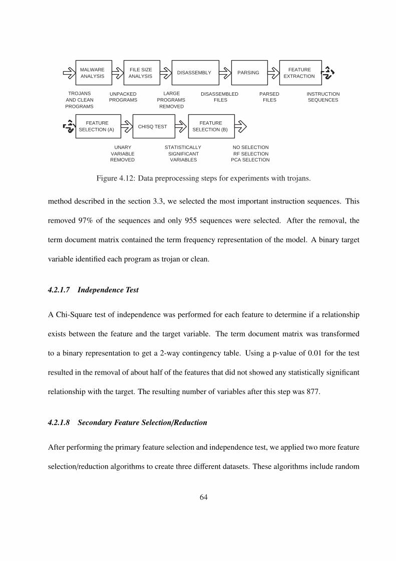
MALWARE ANALYSIS


EXTRACTION

TROJANS AND CLEAN PROGRAMS

UNPACKED PROGRAMS

DISASSEMBLED FILES

PARSED FILES




CHISQ TEST

STATISTICALLY SIGNIFICANT VARIABLES

FILE SIZE ANALYSIS

LARGE PROGRAMS REMOVED

FEATURE SELECTION (B)

NO SELECTION RF SELECTION

PCA SELECTION

Figure 4.12: Data preprocessing steps for experiments with trojans.

method described in the section 3.3, we selected the most important instruction sequences. This

removed 97% of the sequences and only 955 sequences were selected. After the removal, the

term document matrix contained the term frequency representation of the model. A binary target

variable identified each program as trojan or clean.



exists between the feature and the target variable. The term document matrix was transformed

to a binary representation to get a 2-way contingency table. Using a p-value of 0.01 for the test

resulted in the removal of about half of the features that did not showed any statistically significant

relationship with the target. The resulting number of variables after this step was 877.

4.2.1.8 Secondary Feature Selection/Reduction

After performing the primary feature selection and independence test, we applied two more feature

selection/reduction algorithms to create three different datasets. These algorithms include random

64

forest and principal component analysis. The first dataset retained all the original 877 variables. In

the results section 4.2.3, this set is referred to as All variables.

Random Forest: While using the random forest model for feature selection, we rejected the

variables for which the mean decrease in accuracy was less than 10%. Only 84 variables were

selected. In the results section 4.2.3, this set is referred to as RF variables.

Principal Component Analysis: During the PCA feature reduction process, we obtained the

146 variables that explained 95% variance in the dataset and rejected others. In the results section

4.2.3, this set is referred to as PCA variables.

4.2.2 Experiments

The data was partitioned into 70% training and 30% test data. Similar experiments showed best

results with tree based models for the count data [SWL08]. We built bagging and random forest

models using R [R]. We also experimented with SVMs using R.

4.2.2.1 Bagging

Classification trees were used with 100 bootstrap replications in the Bagging model.

4.2.2.2 Random Forest

We grew 100 classification trees in the random forest model. The number of variables sampled at

each split was ranged from 6 to 43 depending upon the number of variables in the dataset.

4.2.2.3 Support Vector Machines

We used C-Classification with a radial basis kernel function.

65

Table 4.6: Experimental results for new and unknown trojans.Classifier Variables Detection Rate False Alarm Rate Overall AccuracyRandom Forest All 93.1% 6.3% 92.6%Random Forest RF 92.4% 9.2% 94.0%Random Forest PCA 89.7% 10.1% 89.6%Bagging All 91.1% 7.4% 89.8%Bagging RF 91.1% 9.6% 91.9%Bagging PCA 89.4% 10.5% 89.4%SVM All 83.6% 15.0% 82.6%SVM RF 83.3% 12.3% 79.7%SVM PCA 82.5% 19.8% 84.7%

1−Specificity

Sen

sitiv

ity

0.0 0.2 0.4 0.6 0.8 1.0

0.0

0.2

0.4

0.6

0.8

1.0

All variablesRF selectionPCA selection

Figure 4.13: ROC curve comparing random forest test results on datasets with all variables, RFvariables and PCA variables.

4.2.3 Results

Like, in the experiments described in the previous section, we tested the models using the 30%test

data. Table 4.6 displays the experimental results for each classifier over the three training sets.

4.2.4 Discussion

Random forest stood out to be the winner among all the classifiers and dimension reduction meth-

ods in our experiments. The best results for overall accuracy, false positive rate and area under

66

1−Specificity

Sen

sitiv

ity

0.0 0.2 0.4 0.6 0.8 1.0

0.0

0.2

0.4

0.6

0.8

1.0

SVMRFBagg

Figure 4.14: ROC curve comparing random forest, bagging and SVM test results on dataset withRF selection.

Table 4.7: Area under the ROC curve for each classifier for each dataset.Classifier Variables AUCRandom Forest All 0.9772Random Forest RF 0.9754Random Forest PCA 0.9537Bagging All 0.9714Bagging RF 0.9686Bagging PCA 0.9549SVM All 0.9295SVM RF 0.9305SVM PCA 0.8971

67

the ROC curve were obtained using random forest classifier on all the variables. The best detec-

tion rate was obtained using random forest model with feature selection using a previous run of

random forest. This comes with a slight sacrifice in overall accuracy but a much simpler model.

Tree based method performed better on the count data. More specifically random forest performed

slightly better than Bagging which is an endorsement of its superiority over Bagging as claimed

in [Bre01]. ROC curves are provided to compare results for each classifier and each dataset. For

space considerations, we are only providing ROC curves for RF Dimensions dataset for each clas-

sifier in figure 4.13. To compare the results over each dataset figure 4.14 displays ROC curve for

random forest test results for the three datasets.

4.3 Worms

Worms claim more damage to the economy than any other type of malware. In the recent years the

most notable malwares were mostly worms including Melissa, ILoveYou, Code Red I & II, Nimda,

SQL Slammer, Blaster, SoBig, Sober, MyDoom, Witty and Sasser worms. The same framework

that we developed for trojans and viruses was extended to include worms.


Our collection of 3195 Windows PE files consisted of 1473 worms and 1722 clean programs. The

clean programs were obtained from a PC running Windows XP. These include small Windows

applications such as calc, notepad, etc and other application programs running on the machine.

A number of clean programs were also downloaded from [Dow] to get a representation of down-

loaded programs. The worms were downloaded from [vx]. The dataset was thus consisted of a

68

Table 4.8: Packers/Compilers Analysis Details of Worms and Clean ProgramsBefore Unpacking After Unpacking

Packer/Compiler Worms Cleans Worms CleansASPack 79 2 1 0Borland 118 39 258 45FSG 31 1 3 0Microsoft 350 937 649 976Other Not Packed 205 597 234 601Other Packed 104 24 135 28PECompact 26 2 7 0Unidentified 161 72 161 72UPX 399 48 24 0Total 1473 1722 1473 1722

Table 4.9: Packers/Compilers Analysis Summary of Worms and Clean ProgramsBefore Unpacking After Unpacking

Packer/Compiler Worms Cleans Worms CleansNot Packed 672 1573 1140 1622Packed 640 77 171 28Unidentified 161 72 162 72Total 1473 1722 1473 1722

wide range of programs, created using different compilers and resulting in a sample set of uniform

representation. Figure 4.17 displays the data processing steps.


We ran PEiD [PEi] on our data collection to detect compilers, common packers and cryptors, used

to compile and/or modify the programs. Table 4.8 displays the distribution of different packers

and compilers in the collection. Before further processing, packed programs were unpacked using

specific unpackers such as UPX (with -d switch) [UPX], and generic unpackers such as Generic

Unpacker Win32 [GUW] and VMUnpacker [VMU]. Table 4.9 displays the summary of packed,

not packed and unidentified trojans and clean programs.

69

Figure 4.15: Portion of the output of disassembled Netsky.A worm.

A number of clean programs were removed to keep an equal class distribution. The unidentified

programs were also removed.

4.3.1.2 Disassembly

Binaries were disassembled to obtain a source code representation using Datarescues’ IDA Pro

[IDA]. Programs with disassembly errors were removed from the dataset.


The core of the Feature Extraction Mechanism consisted of a parser that parsed the disassembled

files to generate instruction sequences. A sequence is defined as instructions in succession until a

conditional or unconditional branch instruction and/or a function boundary is reached. Instruction

sequences thus obtained are of various lengths. We only considered the opcode and the operands

were discarded from the analysis. Figure 4.15 shows a portion of the disassembly of the Netsky.A

worm.

The parser was written in PHP and it translated the disassembly in figure 4.15 to instruction

sequences. Figure 4.16 displays the output of the parser. Each row in the parsed output represented

a single instruction sequence. For comparison purposes we also extracted non-overlapping fixed

70

Figure 4.16: Instruction sequences extracted from the disassembled Netsky.A worm.

MALWARE ANALYSIS


EXTRACTION

WORMS AND CLEAN PROGRAMS

UNPACKED PROGRAMS

DISASSEMBLED FILES

PARSED FILES


AND N-GRAMS



CHISQ TEST

STATISTICALLY SIGNIFICANT VARIABLES

FILE SIZE ANALYSIS

LARGE PROGRAMS REMOVED

FEATURE SELECTION (B)

NO SELECTION RF SELECTION

PCA SELECTION

Figure 4.17: Data preprocessing steps for experiments with worms.

length instruction sequences from the disassembly. These fixed length sequences will be termed

n-grams in this paper, where n is the length of the sequence. The value of n was varied from 2 to

10 in our experiments.

4.3.1.4 Feature Selection/Reduction





method described in the section 3.3, we selected the most important instruction sequences. After

the removal, the term document matrix contained the term frequency representation of the model.

A binary target variable identified each program as worm or clean. We also added a heuristic flag

variable indicating if the worm or clean program was originally found in a packed or an unpacked

71

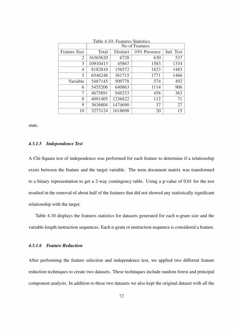
Table 4.10: Features StatisticsNo of Features

Feature Size Total Distinct 10% Presence Ind. Test2 16365620 6728 630 5373 10910413 45867 1583 13344 8182810 156572 1823 14835 6546248 361715 1771 1466

Variable 5487145 509778 574 4926 5455206 640863 1114 9067 4675891 949233 458 3638 4091405 1236822 112 719 3636804 1474690 37 27

10 3273124 1618698 20 15

state.






relationship with the target.

Table 4.10 displays the features statistics for datasets generated for each n-gram size and the

variable length instruction sequences. Each n-gram or instruction sequence is considered a feature.

4.3.1.6 Feature Reduction

After performing the feature selection and independence test, we applied two different feature

reduction techniques to create two datasets. These techniques include random forest and principal

component analysis. In addition to these two datasets we also kept the original dataset with all the

72

Table 4.11: Reduced Feature SetsFeature Size All Variables RF Variables PCA Variables

2 537 79 1243 1334 124 1484 1483 138 1335 1466 138 120

Variable 492 89 1646 906 148 1647 363 99 2008 71 35 689 27 15 27

10 15 10 1520 0 0 0

features retained from the chi-square test output. In the results section 4.4, this dataset is referred

to as All variables.


We followed the same procedure for feature selection using random forest, that we developed for

the trojan dataset. The variables for which the mean decrease in accuracy was less than 10% were

rejected. In the results section 4.4, this dataset is referred to as RF variables

4.3.1.8 Principal Component Analysis

PCA was also employed under the similar conditions. We kept the variables that explained 95%

variance in the dataset and rejected others. In the results section 4.4, this dataset is referred to as

PCA variables

Table 4.11 displays the number of features in each dataset after applying the random forest and

principal component analysis, for each feature size.

73

4.3.2 Experiments

Experiments were conducted on 30 different datasets. As explained in the previous section these

were generated by using a combination of feature size and selection mechanism. Each dataset was

partitioned into 70% training and 30% test data. Similar experiments showed best results with tree

based models for the count data [SWL08]. We built bagging and random forest models using R

[R].

4.3.2.1 Bagging

We used classification trees with 100 bootstrap replications in the Bagging model.


We grew 100 classification trees in the Random forest model. Each random forest model was first

tuned to obtain the optimal number of variables to be sampled at each node.

4.4 Results

As explained in the previous experiments, the 30% test data was used to test the efficiency of the

models. Table 4.12 displays the experimental results for each classifier, selection strategy and

n-gram size combination.

74

Table 4.12: Experimental results for new and unknown

worms.

Classifier Variables Size Detection

Rate

False

Alarm Rate

Overall

Accuracy

Random Forest All variable 94.3% 5.64% 94.24%

Random Forest RF variable 93.85% 7.6% 95.38%

Random Forest RF 5 93.04% 7.46% 93.56%

Random Forest RF 2 92.85% 5.74% 91.47%

Random Forest All 2 92.7% 6.85% 92.29%

Bagging RF 2 92.55% 6.65% 91.76%

Bagging All variable 92.5% 7.12% 92.12%

Bagging RF variable 92.35% 8.48% 93.23%

Random Forest RF 4 91.63% 7.45% 90.78%

Random Forest RF 8 91.63% 7.45% 90.78%

Random Forest RF 9 91.63% 7.45% 90.78%

Bagging RF 5 91.57% 8.28% 91.41%

Random Forest RF 3 91.51% 5.49% 88.63%

Random Forest PCA 4 91.38% 8.06% 90.8%


Continued on next page

75

Table 4.12 – Experimental results for new and unknown worms.


Rate

False

Alarm Rate

Overall

Accuracy








Bagging All 3 90.76% 7.01% 88.63%

Bagging PCA 5 90.62% 10.75% 92.02%

Bagging RF 3 90.61% 7.32% 88.63%

Bagging PCA variable 90.55% 9.5% 90.61%

Random Forest PCA variable 90.4% 8.31% 89.09%

Bagging All 2 90.31% 6.85% 87.71%


Bagging All 5 90.17% 10.15% 90.49%




76



Rate

False

Alarm Rate

Overall

Accuracy

Random Forest RF 7 89.29% 11.21% 89.81%


Bagging PCA 3 89.27% 8.23% 86.88%

Random Forest RF 6 88.7% 10% 87.54%

Bagging RF 4 88.64% 8.7% 86.17%

Bagging RF 8 88.64% 8.7% 86.17%

Bagging RF 9 88.64% 8.7% 86.17%

Bagging RF 6 88.55% 7.42% 84.93%

Bagging PCA 2 88.23% 13.27% 89.76%

Bagging All 6 87.94% 9.03% 85.22%

Bagging PCA 4 87.29% 13.76% 88.3%

Bagging PCA 6 87.29% 13.76% 88.3%

Bagging PCA 7 87.29% 13.76% 88.3%

Bagging PCA 8 87.29% 13.76% 88.3%

Bagging PCA 9 87.29% 13.76% 88.3%

Bagging RF 7 87.27% 12.12% 86.62%

Bagging All 7 87.11% 13.03% 87.26%


77



Rate

False

Alarm Rate

Overall

Accuracy

Random Forest All 8 81.13% 12.5% 75%

Bagging All 8 80.81% 11.84% 73.73%


Random Forest RF 10 79.66% 12.35% 72.36%

Bagging All 10 78.14% 15.14% 72%


Bagging RF 10 77.76% 15.94% 72%


Bagging PCA 10 77.57% 12.75% 68.73%

Bagging All 9 74.61% 27.92% 76.8%

Table 4.12 indicates that the variable length instruction sequences resulted in a higher detection

and a lower false positive rate than the fixed length instructions of various sizes. Combining the

statistics of table 4.10 with the results of table 4.12, it is also evident that variable length instruction

sequences resulted in a better overall accuracy with a dataset of lesser dimensions, than the fixed

length instruction sequences. Among the classifiers, random forest performed better than bagging

which is endorsement of its superiority over bagging as claimed in [Bre01].

78

1−Specificity

Sen

sitiv

ity

0.0 0.2 0.4 0.6 0.8 1.0

0.0

0.2

0.4

0.6

0.8

1.0

Variable2−Grams3−Grams4−Grams5−Grams6−Grams7−Grams8−Grams9−Grams10−Grams

Figure 4.18: ROC curves comparing random forest results for each n-gram size using all variables.

Figures 4.18 - 4.25 display ROC curves comparing various combinations of classifiers, selec-

tion strategies and n-gram sizes. Figure 4.18 compares ROC curves for each n-gram size using ran-

dom forest classifier on all the variables. Figure 4.19, compares similar curves on the random forest

selection datasets, while figure 4.20, compares ROC curves on the PCA selection datasets. Figures

4.21, 4.22 and 4.23, compare similar ROC curves using bagging as the classification method. Fig-

ure 4.24 compares the results from each classifier on the random forest selected, variable length

instruction sequences dataset. Another area of interest is to compare the different feature selection

and reduction mechanisms used in these experiments. Figure 4.25 compares the ROC curves using

random forest classifier on the variable length instruction sequences dataset using all variables, RF

variables and PCA variables.

79

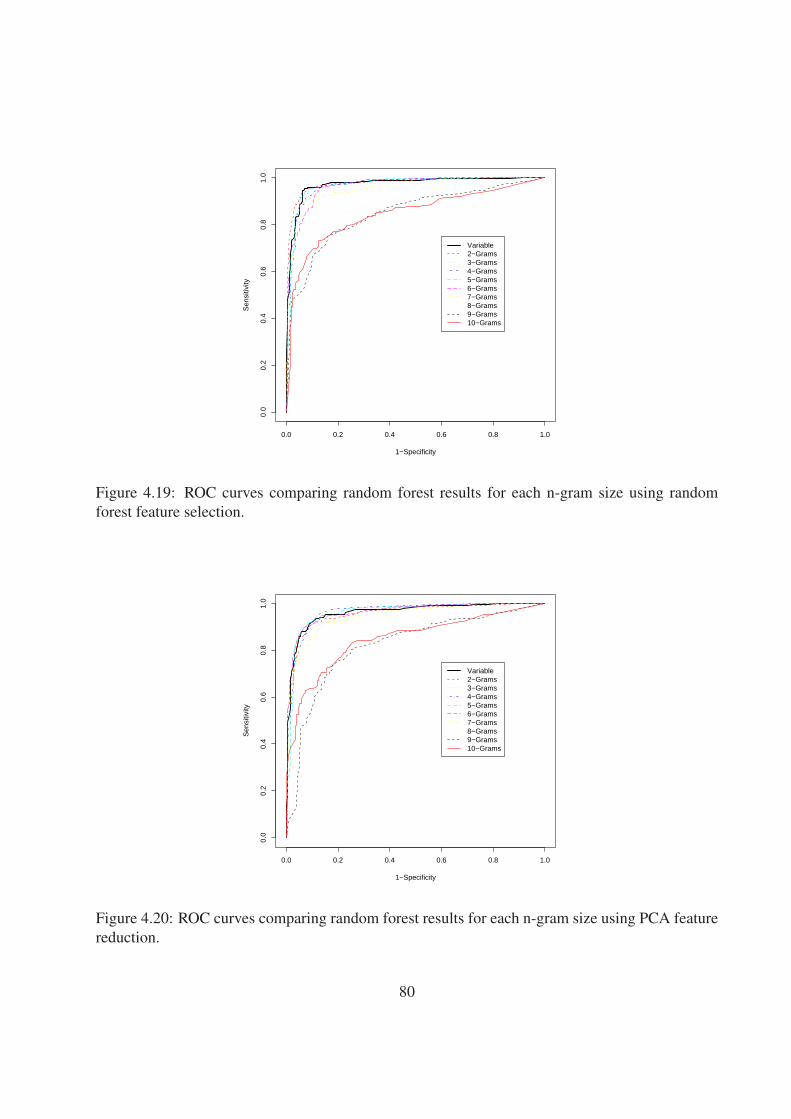
1−Specificity

Sen

sitiv

ity

0.0 0.2 0.4 0.6 0.8 1.0

0.0

0.2

0.4

0.6

0.8

1.0


Figure 4.19: ROC curves comparing random forest results for each n-gram size using randomforest feature selection.

1−Specificity

Sen

sitiv

ity

0.0 0.2 0.4 0.6 0.8 1.0

0.0

0.2

0.4

0.6

0.8

1.0


Figure 4.20: ROC curves comparing random forest results for each n-gram size using PCA featurereduction.

80

1−Specificity

Sen

sitiv

ity

0.0 0.2 0.4 0.6 0.8 1.0

0.0

0.2

0.4

0.6

0.8

1.0


Figure 4.21: ROC curves comparing bagging results for each n-gram size using all variables.

1−Specificity

Sen

sitiv

ity

0.0 0.2 0.4 0.6 0.8 1.0

0.0

0.2

0.4

0.6

0.8

1.0


Figure 4.22: ROC curves comparing bagging results for each n-gram size using random forestfeature selection.

81

1−Specificity

Sen

sitiv

ity

0.0 0.2 0.4 0.6 0.8 1.0

0.0

0.2

0.4

0.6

0.8

1.0


Figure 4.23: ROC curves comparing bagging results for each n-gram size using PCA feature re-duction.

1−Specificity

Sen

sitiv

ity

0.0 0.2 0.4 0.6 0.8 1.0

0.0

0.2

0.4

0.6

0.8

1.0

RFBag

Figure 4.24: ROC curves comparing random forest and bagging results using random forest featureselection.

82

1−Specificity

Sen

sitiv

ity

0.0 0.2 0.4 0.6 0.8 1.0

0.0

0.2

0.4

0.6

0.8

1.0

RFBagPCA

Figure 4.25: ROC curves comparing the variable selection methods (all variables, RF variables,PCA variables)

Table 4.13: Area under the ROC curve for each classifier.

Classifier Variables Size AUC

Random Forest All var 0.9797275

Random Forest All 2 0.9769337

Random Forest RF 2 0.9765461

Bagging All var 0.974773

Random Forest RF var 0.9722357

Bagging RF 2 0.9708548



83

Table 4.13 – Area under the ROC curve for each classifier.







Random Forest PCA 4 0.9640092



Bagging PCA var 0.9625978


Random Forest PCA var 0.961695

Bagging RF var 0.9611786


Bagging All 2 0.9604272






84




Bagging PCA 5 0.9562128


















85











Bagging RF 10 0.8404781








86

CHAPTER 5UNSUPERVISED LEARNING EXPERIMENTS

The unsupervised learning experiments involved using sequential association analysis on the mal-

ware collection. Association analysis is a form of descriptive data mining, where the focus is to

mine the data for patterns that describe association among data elements and are easily understand-

able by humans. It is the most common form of local pattern discovery in an unsupervised learning

environment. Association analysis discovers patterns in the form of association rules that describes

the elements that are frequently found together in the data and assign confidence scores to these

rules.

Association analysis can be best explained by Market Basket Analysis, which searches for

items that are frequently found together in a random market basket. In the malware detection

realm, association analysis can be used to discover features that are found together in each class of

programs, i.e. malware or clean, and use this information for the detection of new and unknown

malwares. Market basket analysis works at transaction level and finds items that are found together

in many transactions. An extension of association analysis is sequential association analysis, that

works at the user level, instead of transaction level. The user level analysis considers all the

transactions done by a specific user in a sequence.

As explained previously, the basic feature for our experiments is a variable length instruction

sequence. Intuitively, sequence mining was the method that we adopted for our experiments,

where each candidate item was an instruction sequence. We devised two types of experiments

using the association analysis for malware detection. One was to use association analysis for

feature extraction/selection and in the second class of experiments we used association analysis

87

for automatic malware signature extraction.

5.1 Feature Extraction

Chapter 4 described the use of occurrence frequency as the main feature selection method. This

section explains the use of sequence mining as the primary feature extraction/selection mechanism.

We used the same collection of malware and clean programs that was used previously in 4.3.

The malware analysis, disassembly and feature extraction steps remained the same. The feature

extraction mechanism was different as we used sequential association mining as the primary feature

extraction/selection method, instead of unary variable removal. Features were originally extracted

from the parsed files. The sequential association mining extracted rules from these features that

can be used as features for a subsequent supervised learning process.


The vector representation of programs was no longer valid in sequence mining as the frequent

instruction sequences were searched globally in the entire data collection, instead of locally, within

a program.

5.1.1.1 Data Partitioning

Malware and clean sequences were separated prior to transforming the data into the form required

by the sequence node in the SAS/Enterprise Miner. This was done because sequence mining is an

unsupervised operation, so a target variable is not included during the process.

88

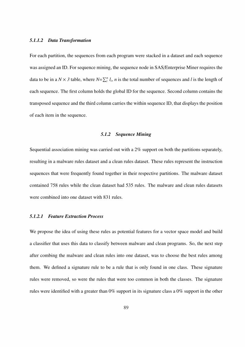
5.1.1.2 Data Transformation

For each partition, the sequences from each program were stacked in a dataset and each sequence

was assigned an ID. For sequence mining, the sequence node in SAS/Enterprise Miner requires the

data to be in a N × 3 table, where N=∑n

i li, n is the total number of sequences and l is the length of

each sequence. The first column holds the global ID for the sequence. Second column contains the

transposed sequence and the third column carries the within sequence ID, that displays the position

of each item in the sequence.

5.1.2 Sequence Mining

Sequential association mining was carried out with a 2% support on both the partitions separately,

resulting in a malware rules dataset and a clean rules dataset. These rules represent the instruction

sequences that were frequently found together in their respective partitions. The malware dataset

contained 758 rules while the clean dataset had 535 rules. The malware and clean rules datasets

were combined into one dataset with 831 rules.

5.1.2.1 Feature Extraction Process

We propose the idea of using these rules as potential features for a vector space model and build

a classifier that uses this data to classify between malware and clean programs. So, the next step

after combing the malware and clean rules into one dataset, was to choose the best rules among

them. We defined a signature rule to be a rule that is only found in one class. These signature

rules were removed, so were the rules that were too common in both the classes. The signature

rules were identified with a greater than 0% support in its signature class a 0% support in the other

89

class. To identify the common rules the absolute difference in the support level in each class was

calculated and a 1% threshold was set, below which every rule was considered as too common,

and hence, rejected. After this step we were left with only 227 rules and that was considered the

final rule set. As explained previously, these rules represent the instruction sequences that were

frequently found together in the malware and clean data.

5.1.2.2 Dataset

We used the vector space model for final dataset representation. Each program was considered a

vector in a n dimensional space where n was the number of features selected using the sequential

association mining procedure described in the last section. A term document matrix was created

where each program represented a document, while rules representing instruction sequences were

considered as terms. A term frequency was computed for each rule within each program. A binary

target variable identified each program as malware or clean. We also added a heuristic flag variable

indicating if the malware or clean program was originally found in a packed or an unpacked state.






relationship with the target.

90

Table 5.1: Experimental results for new and unknown malwares using sequential association anal-ysis as well as a combined selection method.

Classifier Selection Detection Rate False Alarm Rate Overall AccuracyRandom Forest Assoc 66.6% 21.4% 72.1%Random Forest Merged 94.6% 10.2% 92.2%

5.1.3 Experiments

To perform the experiments, we constructed two datasets. The first contained the features selected

from the sequence mining process and another dataset that combined the features selected from the

sequence mining process and the occurrence frequency process. The datasets were partitioned into

70% training and 30% test data. Similar experiments showed best results with tree based models

for the count data [SWL08]. We built random forest models using R [R].


We grew 100 classification trees in the Random forest model. Each random forest model was first

tuned to obtain the optimal number of variables to be sampled at each node.

5.1.4 Results

We tested the model using the 30% test data from both the datasets. Table 5.1 displays the experi-

mental results.

Figure 5.1 compares the ROC curves for the results from the feature set, selected using se-

quence association mining only and the combined feature set with features from sequence associ-

ation mining and occurrence frequency.

It is obvious from table 5.1 and figure 5.1, that the features selected using sequence association

91

1−Specificity

Sen

sitiv

ity

0.0 0.2 0.4 0.6 0.8 1.0

0.0

0.2

0.4

0.6

0.8

1.0

Merged DataAssoc. Data

Figure 5.1: ROC curves comparing the results for the features selected using sequence associationmining only and the combined feature set.

mining cannot be used towards a classification application, alone. The feature set can be merged

with another feature set to create a hybrid set of two distinct feature selection mechanism. The

94.6% detection rate on new and unknown malwares validates this point.

5.2 Automatic Malware Signature Extraction

Signature detection is the industry standard for fighting against malwares [ACK04a]. These sig-

natures are usually hand crafted by security experts. The first known data mining application for

malware detection was for automatic signature extraction by [KA94]. Results were not very im-

pressive but it opened the gate for data mining research in malware detection.

We propose a new idea of based upon association analysis to extract malware signatures. The

underlying idea is to extract instruction sequences that are found frequently in a collection of mali-

92

cious programs and then filter the ones that have any occurrence in a collection of clean programs.

The result will be a generalized set of malware signatures that are not specific to any particular

malware. Such a general set of malware signatures can thwart zero day attacks and do not need

any human expertise.


We used the same collection of malware and clean programs that was used previously in 4.3. The

malware analysis and disassembly steps remained the same. Features were extracted using the

similar process but instead of saving the features from all the programs in one file, this time the

features from each program were saved individually in separate files. No feature selection mech-

anism was used as the vector representation of programs was not used in the signature extraction

scheme. Feature selection was implicit in the signature extraction algorithm. No partitioning is

required for these experiments as individual malware and clean data is used.

5.2.1.1 Data Transformation

Each program was converted from its instruction sequence representation to the conform the re-

quirements of the association node in SAS/Enterprise Miner. For sequence mining, the sequence

node in SAS/Enterprise Miner requires the data to be in a N × 3 table, where N=∑n

i li, n is the total

number of sequences and l is the length of each sequence. The first column holds the global ID for

the sequence. Second column contains the transposed sequence and the third column carries the

within sequence ID, that displays the position of each item in the sequence.

93

5.2.2 Signature Extraction

The signature extraction mechanism used an incremental process to create the signature database.

This databases was built by constantly adding new and unique class signatures from the program

collection and removing the ones that were found in both classes. We performed a series of exper-

iments by modifying the basic signature extraction algorithm for improved efficiency.

5.2.2.1 Basic Algorithm

The basic algorithm creates and updates a malware signature database. The database is updated

every time a new malware signature is found or an existing signature is found in a clean program.

The basic algorithm can be described as,

Input: A Collection of FilesOutput: Malware Signature DatabaseRead a malware file;Run assoc analysis on the file with 0% support;Output the generated rules to create the signature database;for each file do

Read the file;Run assoc analysis on the file with 0% support;Output the generated rules;Search the signature database for the generated rules;if True Positive or True Negative then

Goto next file;endelse if False Positive then

Remove the signature from the signature database;endelse if False Negative then

Add the signature to the signature database;end

endAlgorithm 1: Basic algorithm for signature extraction

The main update is the step where the algorithm searches the signature database for the gen-

94

Table 5.2: Truth table for the basic algorithm.Malware Found Verdict

0 0 TN0 1 FP1 0 FN1 1 TP

erated rules. Four scenarios arise from this situation that are described as a truth table in table

5.2.

Scenario 1: The file being processed is a clean file and no match is found. A true negative (TN)

is generated in this case.

Scenario 2: The file being processed is a clean file and a match is found. A false positive (FP)

is generated in this case.

Scenario 3: The file being processed is a malware file and no match is found. A false negative

(FN) is generated in this case.

Scenario 4: The file being processed is a malware file and a match is found. A true positive

(TP) is generated in this case.

Scenarios 1 and 4 do not trigger any update to the malware database. The update is required

for scenarios 2 and 3. In the case of a false positive, the subject file is a clean file, therefore

the matching signature has to be removed from the malware signature database. Similarly in the

false negative case, the signature has to be added to the signature database, as the subject file is a

malware and the signature database do not carry a matching signature.

The algorithm is nothing more than an online version of the batch processing described in the

feature selection section of 5.1. The main difference is the nature and number of features that were

finally selected. In the feature selection scheme, signatures were removed and only the features

95

that were common to both classes were kept. The signature extraction scheme kept the signatures

belonging to the malware class only. As the signatures are usually rare items, the signature ex-

traction ran the association analysis with 0% support while the feature selection mechanism was

interested in the most frequent features only, therefore the support level was 2%. The experiments

were carried out using SAS/Enterprise Miner on a Pentium 4, 3.0 GHz machine with 1 GB of mem-

ory. Initially the batch version was tried with 0% support but upon receiving memory problems,

the online version of the algorithm had to be developed.

The basic algorithm did not proved to be very efficient in terms of detection rate and false

positive rate. A very high false positive rate of 30% for the test dataset suggested that too many

signatures remained in the malware signature database that should have been filtered. Poor perfor-

mance of the basic algorithm led to the development of the modified algorithm.

5.2.2.2 Modified Algorithm

The basic algorithm was modified to include clean signatures also and a plurality vote on clean and

malware signatures decided if the subject file should be labeled as clean or malware. The modified

algorithm can be described as,

The modified algorithm treated clean programs also as target for clean signatures. This resulted

in two truth tables, one for each class. Table 5.3 gives the truth table for clean programs. In this

table a clean program whose signature is not found in the clean program is considered to be a false

negative. Similarly, table 5.4 gives the truth table for malwares.

These two truth tables can be combined to cover the eight possible scenarios at each iteration

of the algorithm.

96

Input: A Collection of FilesOutput: Malware and Clean Signature DatabasesRead a malware file;Run assoc analysis on the file with 0% support;Output the generated rules to create the malware signature database;Read a clean file;Run assoc analysis on the file with 0% support;Output the generated rules to create the clean signature database;for each file do

Read the file;Run assoc analysis on the file with 0% support;Output the generated rules;Search the malware signature database for the generated rules;Search the clean signature database for the generated rules;if True Positive or True Negative then

Goto next file;endelse if False Positive then

if Subject File is a Malware thenRemove the matching signatures from the malware signature database;

endelse if Subject File is a Clean File then

Remove the matching signatures from the clean signature database;end

endelse if False Negative then

if Subject File is a Malware thenAdd the new signatures to the malware signature database;

endelse if Subject File is a Clean File then

Add the new signatures to the clean signature database;end

endend

Algorithm 2: Modified algorithm for signature extraction

Table 5.3: Truth table for the modified algorithm for clean files.Malware Found Verdict

0 0 FN0 1 TP1 0 TN1 1 FP

97

Table 5.4: Truth table for the modified algorithm for malwares.Malware Found Verdict

0 0 TN0 1 FP1 0 FN1 1 TP

Table 5.5: Truth table for the modified algorithm for malwares and clean programsMalware Found in Clean Found in Malware Clean Malware

0 0 0 FNC TNM0 0 1 FNC TNM0 1 0 FNC TNM0 1 1 FNC TNM1 0 0 FNC TNM1 0 1 FNC TNM1 1 0 FNC TNM1 1 1 FNC TNM

The scenarios described in the table 5.5, are explained below,

Scenario 1: The file being processed is a clean file and no matching signature is found in the

clean signature database and no matching signature is found in the malware signature database.

We defined this as a false negative clean (FNC) and a true negative malware (TNM) situation.

Scenario 2: The file being processed is a clean file and no matching signature is found in the

clean signature database and matching signatures are found in the malware signature database. We

defined this as a false negative clean (FNC) and a false positive malware (FPM) situation.

Scenario 3: The file being processed is a clean file and matching signatures are found in the

clean signature database and no matching signature is found in the malware signature database.

We defined this as a true positive clean (TPC) and a true negative malware (TNM) situation.

Scenario 4: The file being processed is a clean file and matching signatures are found in the


98

defined this as a true positive clean (TPC) and a false positive malware (FPM) situation.

Scenario 5: The file being processed is a malware file and no matching signature is found in

the clean signature database and no matching signature is found in the malware signature database.

We defined this as a true negative clean (TNC) and a false negative malware (FNM) situation.

Scenario 6: The file being processed is a malware file and no matching signature is found in

the clean signature database and matching signatures are found in the malware signature database.

We defined this as a true negative clean (TNC) and a true positive malware (TPM) situation.

Scenario 7: The file being processed is a malware file and matching signatures are found in

the clean signature database and no matching signature is found in the malware signature database.

We defined this as a false positive clean (FPC) and a false negative malware (FNM) situation.

Scenario 8: The file being processed is a malware file and matching signatures are found in the


defined this as a false positive clean (FPC) and a true positive malware (TPM) situation.

5.2.3 Results

The basic algorithm was not able to stand the test for new and unknown malwares and gave a high

false positive rate of around 30%. This indicated the flaw in the filtering method as only those

signatures were filtered out that were found in the training data. A high number of signatures were

found in the clean programs in the test dataset. The modified algorithm remedied this problem.

Assigning the final class outcome based upon the majority vote for malware and clean signatures in

a file decreased the false positive rate significantly. Besides counts of the signatures, the signature

databases also carried the scores for each signature that described the probability of finding that

99

Table 5.6: Experimental results for new and unknown malwares using automatically extractedsignatures by applying sequential association mining.

Method Detection Rate False Alarm Rate Overall AccuracyCount 73.1% 2.2% 85.9%Score 85.9% 7.0% 89.6%Combined 86.5% 1.9% 92.5%

signature in the entire program collection. Besides count of the signatures, we used these scores

also to reach a final class verdict. The last measure that we used was a combination of scores and

counts.

100

CHAPTER 6CONCLUSIONS

This dissertation provided an introduction to the malware research using data mining techniques.

We applied a four tier hierarchy to organize the research and included data mining in the top tier of

detection methods. Our work closely resembles information retrieval and classification techniques,

where we replaced text documents with computer programs and applied similar techniques. Un-

like previous attempts at applying data mining techniques at a syntactic level, using n-grams, we

introduced a variable length instruction sequence, that inherently captures program control flow in-

formation and hence provides a semantic level interpretation to the program analysis. In our quest

to choose the best classification model, we compared different feature selection methods and clas-

sifiers and provided empirical results. We proposed using association analysis for feature selection

and automatic signature extraction and were able to receive as low as 1.9% false positive rate and

as high as 93% overall accuracy on novel malwares with the algorithms that we devised. In the end

future work is proposed to extend the association analysis method for improved classification and

time and space complexity for the algorithms.

101

CHAPTER 7FUTURE WORK

The malware detection using association analysis research is still in its initial stages. There are

many ideas and methods that are yet to be implemented. We present a number of ideas as future

research directions for using association analysis for malware detection.

7.1 Feature Extraction

Association analysis did not prove to be very effective for feature selection from malware and clean

files. The selected features performed poorly when used alone to classify between new unknown

malware and clean programs. Although we removed signature features and features that were too

common to both the classes, the performance was still poor.

For experimentation purposes, several other representations of the term document matrix that

resulted after the feature selection process, can be used. These include a normalized term count by

total number of terms or by the maximum number of terms. A log scale can also be used, but the

most notable representation is the TF-IDF representation. In the vector space model with a term

frequency or boolean representation, each coordinate of the document vector is computed locally,

taking into account only the particular term and document. This gives equal importance to all the

coordinates, that may not be the case. Some terms occur frequently in a number of documents,

but they may not be related to the defining contents of the document. On the other hand, there

may be terms that are not found in many documents, but may provide a better definition of the

document. This can be cured by the Inverse Document Frequency (IDF) method, that scales down

the contribution of frequent terms across the documents and scales up the rare terms. IDF is

102

multiplied by TF, to get the feature representation. A series of experiments can be conducted for

these representation types.

7.2 Signature Extraction

The signature extraction method needs improvement on two grounds. First is to increase the de-

tection rate and second is to reduce the time and space complexity of the algorithm. The combined

measure of signature scores and count proved efficient with false positives but false negatives re-

mained high and that amounts for a bigger problem.

Signatures are essentially rare items and this should be the direction, the extraction mechanism

should proceed. Traditionally association analysis, gives the items that frequently occur together.

To extract the signatures as rare items, the negative border can be considered, where negative

border is the set of all infrequent items, that were rejected at each step. This would automatically

improve the space complexity.

We used SAS for the sequential association analysis that uses Apriori algorithm to perform the

task. It has been proven that the Apriori, is not the most efficient method for sequential pattern

analysis [Kan02]. For improved efficiency, Frequent Pattern-Growth (FP-Growth) method should

be used instead.

7.3 PE Header

Another area of experimentation is to use the information from the PE header. We initially de-

veloped a rule based system to detect malwares [SWL05]. Instead of using hand crafted heuristic

rules, association analysis can be employed to extract these rules from the malicious PE headers.

103

7.4 Stratified Sampling

We did a random sampling to create training and test datasets with a holdout method with 70/30

split. For a better representation of the various malware families and variants a stratified sampling

approach can be applied. A temporal element can be added to the sampling procedure to reflect

the timeline of the appearance of different malwares. Malwares appearing later in a chronological

sequence of events should be part of test sample to represent newer malwares.

7.5 Real Time Implementation

This work was focused on academic research and the real time implementation of the proposed

data mining framework for malware detection was not discussed. The following issues needs to be

considered for a real time implementation of such a system.

7.5.1 Time and Space Complexity:

The major hindrance for such the real time implementation of such a data mining framework

is the time and space complexity of the machine learning and other algorithms involved. The

disassembly, parsing and feature extraction are time consuming processes and require a lot of space

also. In an automated framework these processes need to be streamlined for better efficiency.

7.5.2 Cost Sensitive Learning:

One thing that was not discussed in this work, is cost sensitiveness of the learning process. False

negatives carry a different cost than false positives. Leaving out a computer virus is not the same as

wrongly identifying a clean program as a virus. To address the issue, cost sensitive learning can be

104

used, where a cost matrix can be defined carrying costs for different true and false identifications.

7.5.3 Class Distribution:

In the malware or fraud detection realm, the class distributions are highly skewed [PAL04], [BJL08].

Cost sensitive learning mentioned in the last paragraph, addresses this issue also. Other methods

include under sampling and over sampling. [MB02].

7.6 Combining Classifiers

In this work, we compared different classifiers and gave experimental results for the best one based

upon classification accuracy and ROC curves. [Web05] gave an excellent account of combin-

ing classifiers. Using this approach we can combine the output of different classifiers instead of

choosing the best one among them. The classifiers can be trained on the same dataset or different

datasets. For different datasets, one suggestion is, to combine the classifiers learned on PE header

information and instruction sequences to assign one final class to the output. For the same dataset,

several classifiers including random forest and neural networks, can be built and the final class

output can be assigned using a voting strategy.

7.7 More Classifiers

We covered an array of classifiers in out work. These include random forest, bagging, decision

tree, neural networks, support vector machines and logistic regression. Several other classifiers

can be added to this list including logic regression (using the Boolean representation of the term-

document matrix), Bayesian methods and nearest neighbor methods.

105

LIST OF REFERENCES

[ACK04a] Tony Abou-Assaleh, Nick Cercone, Vlado Keselj, and Ray Sweidan. “Detection ofnew malicious code using n-grams signatures.” In Proceedings of Second Annual Con-ference on Privacy, Security and Trust, pp. 193–196, 2004.

[ACK04b] Tony Abou-Assaleh, Nick Cercone, Vlado Keselj, and Ray Sweidan. “N-Gram-BasedDetection of New Malicious Code.” In Proceedings of the 28th Annual InternationalComputer Software and Applications Conference - Workshops and Fast Abstracts -(COMPSAC’04) - Volume 02, pp. 41–42, 2004.

[api] “Wikipedia API article. http://en.wikipedia.org/wiki/Api.”.

[AT00] William Arnold and Gerald Tesauro. “Automatically Generated Win32 Heuristic VirusDetection.” In Virus Bulletin Conference, pp. 123–132, 2000.

[BDD99] J. Bergeron, M. Debbabi, J. Desharnais, B. Ktari, M. Salois, and N. Tawbi. “Detectionof Malicious Code in COTS Software: A Short Survey.” In Proceedings of the 1stInternational Software Assurance Certification Conference (ISACC’99), 1999.

[BDD01] J. Bergeron, M. Debbabi, J. Desharnais, M. M. Erhioui, Y. Lavoie, and N. Tawbi.“Static Detection of Malicious Code in Executable Programs.” Symposium on Re-quirements Engineering for Information Security (SREIS’01), 2001.

[BDE99] J. Bergeron, M. Debbabi, M. M. Erhioui, and B. Ktari. “Static Analysis of BinaryCode to Isolate Malicious Behavior.” In Proceedings of the 8th Workshop on EnablingTechnologies on Infrastructure for Collaborative Enterprises (WETICE’99), pp. 184–189, 1999.

[BJL08] Martin Boldt, Andreas Jacobsson, Niklas Lavesson, and Paul Davidsson. “AutomatedSpyware Detection Using End User License Agreements.” isa, 0:445–452, 2008.

[Bon93] Vesselin Bontchev. “Analysis and maintenance of a clean virus library.” In Proceedingsof the 3rd Internation Virus Bulletin Conference, pp. 77–89, 1993.

[Bon96] Vesselin Bontchev. “Possible Virus Attacks Against Integrity Programs and How toPrevent Them.” In Proceedings of the 6th Internation Virus Bulletin Conference, pp.97–127, 1996.

[Bre96] Leo Breiman. “Bagging Predictors.” Machine Learning, 24(2):123–140, 1996.

[Bre01] Leo Breiman. “Random Forests.” Machine Learning, 45(1):5–32, 2001.

[Bru75] John Brunner. Shockwave Rider. Del Rey Books, 1975.

[CJS05] M. Christodorescu, S. Jha, S. Seshia D. Song, and R. Bryant. “Semantics-Aware Mal-ware Detection.” In Proceedings of the 2005 IEEE Symposium on Security and Privacy,pp. 32–46, 2005.

106

[Coh84] Fred Cohen. “Experiments with Computer Viruses.” 1984.

[Coh85] Fred Cohen. Computer Viruses. PhD thesis, University of Southern California, 1985.

[Coh91] Fred Cohen. “A cost analysis of typical computer viruses and defenses.” Computersand Security, 10(3):239–250, 1991.

[Coh94] Fred Cohen. A Short Course on Computer Viruses. Wiley; 2 edition, 1994.

[Cor99] Microsoft Corporation. Microsoft Portable Executable and Common Object File For-mat Specification. Microsoft Corporation, 6 edition, 1999.

[DGP01] M. Debbabi, M. Girard, L. Poulin, M. Salois, , and N. Tawbi. “Dynamic Monitoring ofMalicious Activity in Software Systems.” In Symposium on Requirements Engineeringfor Information Security (SREIS’01), 2001.

[Dow] “Download.com http://www.download.com/.”.

[EAA04] D. Ellis, J. Aiken, K. Attwood, and S. Tenaglia. “A Behavioral Approach to WormDetection.” In Proceedings of the 2004 ACM Workshop on Rapid Malcode, pp. 43–53,2004.

[Ell03] Dan Ellis. “Worm Anatomy and Model.” In Proceedings of the 2003 ACM workshopon Rapid malcode WORM ’03, pp. 42–50, 2003.

[Fer92] David Ferbrache. A Pathology of Computer Viruses. Springer-Verlag, 1992.

[FPM92] W. Frawley, G. Piatetsky-Shapiro, and C. Matheus. “Knowledge Discovery inDatabases: An Overview.” AI Magazine, pp. 213–228, 1992.

[Ger72] David Gerrold. When Harlie Was One. Doubleday, 1972.

[Gry99] Dmitry Gryaznov. “Scanners of the Year 2000: Heuristics.” In Proceedings of the 5thInternational Virus Bulletin Conference, pp. 225–234, 1999.

[Gut07] Peter Gutmann. “The Commercial Malware Industry.”, 2007.

[GUW] “Generic Unpacker Win32. http://www.exetools.com/unpackers.htm.”.

[HFS98] S. Hofmeyr, S. Forrest, and A. Somayaji. “Intrusion detection using sequences ofsystem calls.” Journal of Computer Security, pp. 151–180, 1998.

[HH01] D. Hand and P. Smyth H. Mannila. Principles of Data Mining. MIT Press, 2001.

[HJ06] Olivier Henchiri and Nathalie Japkowicz. “A Feature Selection and Evaluation Schemefor Computer Virus Detection.” icdm, 0:891–895, 2006.

[IDA] “IDA Pro Disassembler. http://www.datarescue.com/idabase/index.htm.”.

107

[IM07] Nwokedi Idika and Aditya P. Mathur. “A Survey of Malware Detection Techniques.”Technical report, Software Engineering Research Center, 2007.

[JH90] Lance J.Hoffman. Rogue Programs: Viruses,Worms, and Trojan Horses. Van NostrandReinhold, 1990.

[KA94] Jeffrey O. Kephart and Bill Arnold. “Automatic Extraction of Computer Virus Signa-tures.” In Proceedings of the 4th Virus Bulletin Internation Conference, pp. 178–184,1994.

[Kan02] Mehmed Kantardzic. Data Mining: Concepts, Models, Methods, and Algorithms.Wiley-IEEE Press, 2002.

[KM04] Jeremy Z. Kolter and Marcus A. Maloof. “Learning to Detect Malicious Executablesin the Wild.” In Proceedings of the 2004 ACM SIGKDD International Conference onKnowledge Discovery and Data Mining, 2004.

[KRL97] C. Ko, M. Ruschitzka, and K. Levitt. “Execution Monitoring of Security-Critical Pro-grams in Distributed Systems: A Specification-Based Approach.” In Proceedings ofthe 1997 IEEE Symposium on Security and Privacy, 1997.

[KWL05] Md. Enamul Karim, Andrew Walenstein, Arun Lakhotia, and Laxmi Parida. “Malwarephylogeny generation using permutations of code.” Journal in Computer Virology,1(1,2):13–23, 2005.

[LLO95] Raymond W. Lo, Karl N. Levitt, and Ronald A. Olsson. “MCF: A Malicious CodeFilter.” Computers and Security, 14(6):541–566, 1995.

[MB02] M. C. Monard and G. E. A. P. A. Batista. “Learning with Skewed Class Distributions.”In J. M. Abe and J. I. da Silva Filho, editors, Advances in Logic, Artificial Intelligenceand Robotics, pp. 173–180, Sao Paulo, SP, 2002. IOS Press.

[MKT07] Mohammad M. Masud, Latifur Khan, and Bhavani Thuraisingham. “A scalable multi-level feature extraction technique to detect malicious executables.” Information Sys-tems Frontiers, 2007.

[ML07] Zdravko Markov and Daniel T. Larose. Data Mining the Web: Uncovering Patterns inWeb Content, Structure, and Usage. Wiley-Interscience, 2007.

[Mor04] Akira Mori. “Detecting Unknown Computer Viruses - A New Approach -.” LectureNotes in Computer Science, pp. 226–241, 2004.

[MP05] W. Masri and A. Podgurski. “Using Dynamic Information Flow Analysis to DetectAgainst Applications.” In Proceedings of the 2005 Workshop on Software Engineeringfor secure sytems Building Trustworthy Applications, 2005.

108

[MS05] David J. Malan and Michael D. Smith. “Host-based detection of worms through peer-to-peer cooperation.” In WORM ’05: Proceedings of the 2005 ACM workshop onRapid malcode, pp. 72–80. ACM, 2005.

[Naz04] Jose Nazario. Defense and Detection Strategies against Internet Worms. Van NostrandReinhold, 2004.

[PAL04] Clifton Phua, Damminda Alahakoon, and Vincent Lee. “Minority report in fraud de-tection: classification of skewed data.” SIGKDD Explor. Newsl., 6(1):50–59, 2004.

[PEi] “PEiD. http://peid.has.it/.”.

[R] “The R Project for Statistical Computing http://www.r-project.org/.”.

[Rad92] Y. Radai. “Checksumming Techniques for Anti-Viral Purposes.” In Proceedings of theIFIP 12th World Computer Congress on Education and Society - Information Process-ing ’92 - Volume 2, pp. 511–517, 1992.

[RKL03] Jesse C. Rabek, Roger I. Khazan, Scott M. Lewandowski, and Robert K. Cunningham.“Detection of Injected, Dynamically Generated, and Obfuscated Malicious Code.” InProceedings of the 2003 ACM Workshop on Rapid Malcode, pp. 76–82, 2003.

[SB99] R. Sekar, T. Bowen, , and M. Segal. “On Preventing Intrusions by Process BehaviorMonitoring.” In USENIX Intrusion Detection Workshop, 1999.

[SBB01] R. Sekar, M. Bendre, P. Bollineni, and D. Dhurjati. “A Fast Automaton-Based Ap-proach for Detecting Anomalous Program Behaviors.” In IEEE Symposium on Securityand Privacy, 2001.

[Sch98] Fred Schneider. “Enforceable Security Policies.” Technical report, 1998.

[SEZ01a] Matthew G. Schultz, Eleazar Eskin, Erez Zadok, Manasi Bhattacharyya, and Salva-tore J. Stolfo. “MEF: Malicious Email Filter: A UNIX Mail Filter That Detects Mali-cious Windows Executables.” pp. 245–252, 2001.

[SEZ01b] Matthew G. Schultz, Eleazar Eskin, Erez Zadok, and Salvatore J. Stolfo. “Data MiningMethods for Detection of New Malicious Executables.” In Proceedings of the IEEESymposium on Security and Privacy, pp. 38–49, 2001.

[SH82] John F. Shoch and Jon A. Hupp. “The Worm Program-Early Experience with a Dis-tributed Computation.” 25(3):172–180, 1982.

[SL02] Prabhat K. Singh and Arun Lakhotia. “Analysis and Detection of Computer Virusesand Worms: An Annotated Bibliography.” SIGPLAN Not., 37(2):29–35, 2002.

[Spa94] Eugene H. Spafford. “Computer Viruses as Artificial Life.” Technical report, 1994.

[SWL05] Muazzam Siddiqui, Morgan C. Wang, and Joohan Lee. “A Rule Based System toDetect Malicious Programs.” Technical report, University of Central Florida, 2005.

109

[SWL08] Muazzam Siddiqui, Morgan C. Wang, and Joohan Lee. “Data Mining Methods forMalware Detection Using Instruction Sequences.” In Proceedings of Artificial Intelli-gence and Applications, AIA 2008. ACTA Press, 2008.

[SXC04] A. H. Sung, J. Xu, P. Chavez, and S. Mukkamala. “Static Analyzer of Vicious Exe-cutables.” In 20th Annual Computer Security Applications Conference, pp. 326–334,2004.

[Sym96] Symantec. “Understanding and Managing Polymorphic Viruses.” Technical report,Symantec Corporation, 1996.

[Sym97] Symantec. “Understanding Heuristics: Symantec’s Bloodhound Technology.” Techni-cal report, Symantec Corporation, 1997.

[Szo05] Peter Szor. The Art of Computer Virus Research and Defense. Addison Wesley forSymantec Press, New Jersey, 2005.

[TKS96] Gerald J. Tesauro, Jeffrey O. Kephart, and Gregory B. Sorkin. “Neural Network forComputer Virus Recognition.” IEEE Expert, 11(4):5–6, 1996.

[UPX] “UPX the Ultimate Packer for eXecutables. http://www.exeinfo.go.pl/.”.

[VMU] “VMUnpacker. http://dswlab.com/d3.html.”.

[vx] “VX Heavens. http://vx.netlux.org.”.

[WD01] D. Wagner and D. Dean. “Intrusion detection via static analysis.” IEEE Symposium onSecurity and Privacy, 2001.

[Web05] Andrew Webb. Statisitcal Pattern Recognition. Wiley, 2005.

[WHS06] Tzu-Yen Wang, Shi-Jinn Horng, Ming-Yang Su, Chin-Hsiung Wu, Peng-Chu Wang,and Wei-Zen Su. “A Surveillance Spyware Detection System Based on Data MiningMethods.” In Evolutionary Computation, 2006. CEC 2006. IEEE Congress on, pp.3236– 3241. IEEE, 2006.

[WPS03] Nicholas Weaver, Vern Paxson, Stuarts Staniford, and Robert Cunningham. “A Tax-onomy of Computer Worms.” In Proceedings of the 2003 ACM workshop on Rapidmalcode WORM ’03, pp. 11–18, 2003.

[WS05] K.Wang W. Li and, S. Stolfo, , and B. Herzog. “Fileprints: Identifying File Types byn-gram Analysis.” In 6th IEEE Information Assurance Workshop, 2005.

[WSS02] Michael Weber, Matthew Schmid, Michael Schatz, and David Geyer. “A Toolkit forDetecting and Analyzing Malicious Software.” In Proceedings of the 18th AnnualComputer Security Applications Conference, p. 423, 2002.

110

[Yoo04] InSeon Yoo. “Visualizing windows executable viruses using self-organizing maps.” InProceedings of the 2004 ACM workshop on Visualization and data mining for computersecurity, pp. 82–89, 2004.

[YP97] Yiming Yang and Jan O. Pedersen. “A Comparative Study on Feature Selection inText Categorization.” In Proceedings of the Fourteenth International Conference onMachine Learning, pp. 412–420, 1997.

[YU06] InSeon Yoo and Ulrich Ultes-Nitsche. “Non-Signature Based Virus Detection: To-wards Establishing Unknown Virus Detection Technique Using SOM.” Journal inComputer Virology, 2(3):163–186, 2006.

[YWL07] Yanfang Ye, Dingding Wang, Tao Li, and Dongyi Ye. “IMDS: intelligent malwaredetection system.” In KDD ’07: Proceedings of the 13th ACM SIGKDD internationalconference on Knowledge discovery and data mining, pp. 1043–1047. ACM, 2007.

111

data mining methods for malware detection

Documents