data-driven risk assessment for truckload service providers
TRANSCRIPT
Data-driven Risk Assessment for Truckload Service Providers
by
Sriram Kishore ChittellaB.A. Sc. Systems Design Engineering, University of Waterloo, 2011
and
ARCHNESMASSACHUSETTP INSTITUTE
OF TECHNOLOLGY
JUL 16 2015
LIBRARIES
Marcos Machado TeixeiraB.S. Economics, FAE Franciscan University Center of Parana, 2005
B.A. Law, Federal University of Parana, 2004
Submitted to the Engineering Systems Division in Partial Fulfillment of theRequirements for the Degree of
Master of Engineering in Logistics
at the
Massachusetts Institute of Technology
June 2015
2015 Kishore Chittella and Marcos Machado Teixeira. All rights reserved.The authors hereby grant to MIT permission to reproduce and to distribute publicly paper andelectronic copies of this document in whole or in part in any medium now known or hereaftercreated. % A
Signature of Author
Signature of Author
Certified by......
Accepted by....
Signature redactedMaster of Engineering in Logistics Program, Engineering Systems Division
. .May 8, 2015
Signature redacted -..................... .. ................----Master of Engineering in Logistics Progrim, Engineering Systems Division
May 8. 2015
Signature redactedDr. Daniel W. Steeneck
Postdoctoral Associate, Cen er for Transportation & Logistics- / Thesis Supervisor
tignature redacted1'
V Dr. Yossi SheffiDirector, Center for Transportation and LogisticsElisha Gray II Professor of Engineering SystemsProfessor, Civil and Environmental Engineering
1
Data-driven Risk Assessment for Truckload Service Providers
by
Sriram Kishore Chittella
and
Marcos Machado Teixeira
Submitted to the Engineering Systems Division on May 8, 2015
in Partial Fulfillment of the Requirements for
the Degree of Master of Engineering in Logistics
ABSTRACT
Non-asset backed third-party logistics companies provide shippers access to a flexiblesource of capacity through transportation carrier spot market. The increased volatility inthe trucking spot market rates is turning the 3PL businesses more risky and complex. Tomaximize profitability, a better understanding of the risk and the volatility patterns acrossthe different geographies, time periods and other factors are investigated based on threeyears of real spot market data from a major 3PL company in US. Throughout thisresearch we investigate the nature of trucking spot market volatility to allow truckloadservice providers to reduce their risk when setting long-term contracts. Using threedifferent measures of volatility we are able to assess the company's risk profile and arisewith insights to improve truckload service providers' business.
Thesis Supervisor: Dr. Daniel SteeneckTitle: Postdoctoral Associate, Center for Transportation & Logistics
2

ACKNOWLEDGEMENTS
We would like to thank Dr. Daniel Steeneck, our thesis advisor, and Dr. ChrisCaplice, our thesis co-advisor, for their brilliant insights throughout the project. Theirguidance and encouragement gave us the necessary fuel to go further and enrich ourlearning experience through this research.
We would like to thank our thesis sponsor company who provided us with thisexciting topic, especially those who worked very close to us contributing to the success ofthis project.
We would like to thank all of the SCM Class of 2015 for the most memorableexperience in our lives, making this year unique and unforgettable.
Kishore Chittella & Marcos Machado Teixeira
I would personally like to thank my family for always encouraging me in myongoing adventures and specially my wife for her love and constant support.
Marcos Machado Teixeira
I thank my family for their love and encouragement. I thank my friends for theirongoing support and my colleagues (academic and industry) for professional developmentopportunities.
Sriram Kishore Chittella
3
Table of Contents
ABSTRACT ........................................................................................................ 2
ACKNOW LEDGEM ENTS ............................................................................... 3
1. INTRODUCTION.................................................................................... 8
2. BACKGROUND ...................................................................................... 11
2.1. Trucking Industry.................................................................................. 11
2.2. Shippers ................................................................................................... 12
2.3. Carriers.................................................................................................... 13
2.4. 3PLs and Brokers.................................................................................... 15
2.5. Methods of Procurement of Truckload Transportation ..................... 17
2.6. Trucking Spot M arket........................................................................... 18
3. LITERATURE REVIEW ...................................................................... 21
3.1. Introduction: Opportunity for Improved Profitability....................... 21
3.2. Price Volatility in Spot M arket.............................................................. 22
3.3. Factors Contributing to Price Volatility in Spot Market .................... 23
3.4. Volatility Patterns .................................................................................... 25
3.5. M athematical Analysis ........................................................................... 26
3.6. Conclusion: Cross Industry Insights.................................................... 27
4. M ETHODOLOGY AND DATASET .................................................... 28
4.1. The Dataset............................................................................................. 28
4.2. Data Preparation.................................................................................... 29
4
4.3. M easures of Volatility............................................................................. 32
4.4. Lane Characterization........................................................................... 35
4.5. Factors Related to Volatility .................................................................. 36
4.6. Linear Regression ................................................................................... 36
4.7. Chapter sum m ary .................................................................................... 38
5. RESULTS ............................................................................................... 39
5.1. Data Exploration.................................................................................... 39
5.2. Distribution of Linehaul Cost per M ile................................................ 43
5.3. V olatility and Correlation ...................................................................... 45
5.4. Lane Characterization........................................................................... 53
5.5. Factors Related to Volatility .................................................................. 54
5.6. Regression Analysis ............................................................................... 66
6. INSIGHTS AND CONCLUSION ........................................................ 68
6.1. K ey Findings........................................................................................... 68
6.2. M anagem ent Im plem entation................................................................ 71
6.3. Recom m endations and Conclusion ...................................................... 75
6.4. Future Research ...................................................................................... 76
REFERENCES .................................................................................................. 78
APPENDIX ...................................................................................................... 80
5
List of TablesT able 1: D ata attributes................................................................................................. 29T able 2: D ata cleaning ................................................................................................... 30Table 3: Beta value interpretation................................................................................. 34Table 4: Regional and national average and coefficient of variation ........................... 42Table 5: Regional probability density functions.......................................................... 44Table 6: Regional beta values (in comparison with national index)............................. 46Table 7: Average month over month percentage changes ............................................. 48Table 8: Correlation of national and regional indices (all data) ................................... 48Table 9: Correlation of national and regional indices (2012)........................................ 49Table 10: Correlation of national and regional indices (2013)...................................... 50Table 11: CASS beta values in comparison with national and regional indices ....... 51Table 12: Correlation of national and regional indices with CASS index (all data) ........ 51Table 13: Region p-values - beta vs. distance............................................................... 55Table 14: Region p-values - coefficient of variation vs. distance................................ 56Table 15: Region p-values - beta vs. volume............................................................... 57Table 16: Region p-values - coefficient of variation vs. volume ................................. 59Table 17: Regression analysis summary...................................................................... 66Table 18: Top risky lanes for ABC company ............................................................... 70Table 19: Top 10 risky long-haul lanes 2012 and 2013 (beta) ..................................... 80Table 20: Top 10 risky long-haul lanes 2012 and 2013 (coefficient of variation)..... 80Table 21: Top 10 risky long-haul lanes 2012 and 2013 (average monthly percentagech an g e).............................................................................................................................. 8 1Table 22: Top 10 risky short-haul lanes 2012 and 2013 (beta) ..................................... 81Table 23: Top 10 risky short-haul lanes 2012 and 2013 (coefficient of variation) ..... 82Table 24: Top 10 risky short-haul lanes 2012 and 2013 (average monthly percentagech an g e).............................................................................................................................. 82Table 25: Top 10 less risky long-haul lanes 2012 and 2013 (beta)............................... 83Table 26: Top 10 less risky long-haul lanes 2012 and 2013 (coefficient of variation) .... 83Table 27: Top 10 less risky long-haul lanes 2012 and 2013 (average monthly percentagech an g e).............................................................................................................................. 84Table 28: Top 10 less risky short-haul lanes 2012 and 2013 (beta) .............................. 84Table 29: Top 10 less risky short-haul lanes 2012 and 2013 (coefficient of variation) ... 85Table 30: Top 10 less risky long-haul lanes 2012 and 2013 (average monthly percentagech an g e).............................................................................................................................. 8 5
6
List of FiguresFigure 1: Third party logistics and broker business........................................................ 8Figure 2: Petroleum administration for defense districts map ...................................... 32Figure 3: Commodity activity by region map (provided by ABC company)............... 37Figure 4: Average cost per mile including fuel costs ................................................... 39Figure 5: N ational index .............................................................................................. 40Figure 6: Regional indices and national index............................................................. 41Figure 7: Regional line haul probability distributions ................................................. 45Figure 8: Volatility by beta of regional indices (in comparison with national index)...... 47Figure 9: Lane characterization framework ................................................................. 53Figure 10: B eta vs. distance.......................................................................................... 54Figure 11: Coefficient of variation vs. distance............................................................. 55Figure 12: B eta vs. volum e ............................................................................................ 57Figure 23: Coefficient of variation vs. volume............................................................. 58Figure 14: National risk profile (2012 and 2013 beta) ................................................. 60Figure 15: Regional risk profile (2012 and 2013 beta).................................................. 60Figure 16: National risk profile (2012 and 2013 coefficient of variation) .................... 62Figure 17: Regional risk profile (2012 and 2013 coefficient of variation).................... 63Figure 18: National risk profile (2012 and 2013 average M/M % change).......... 64Figure 19: Regional risk profile (2012 and 2013 average M/M % change).......... 65Figure 20: Monthly cost per mile - Laredo x Houston (lane 780 - 770) ...................... 72Figure 21: Weekly cost per mile - Laredo x Houston (lane 780 - 770)........................ 73Figure 22: Daily cost per mile - Laredo x Houston (lane 780 - 770)........................... 73Figure 23: Probability density function - Burr (Laredo x Houston) ............................. 74
7
1. INTRODUCTION
The trucking spot market is a marketplace where loads are negotiated on a non-
contract basis. The motivation for this thesis originates from limitations for truckload
service providers in understanding volatility in the trucking spot market. When referring
to truckload service providers, in this research, we mean freight brokers and 3PL (third
party logistics) companies. 3PL is an outsourced provider of activities related to logistics
and distribution, while a freight broker is fundamentally an entity that connects shippers
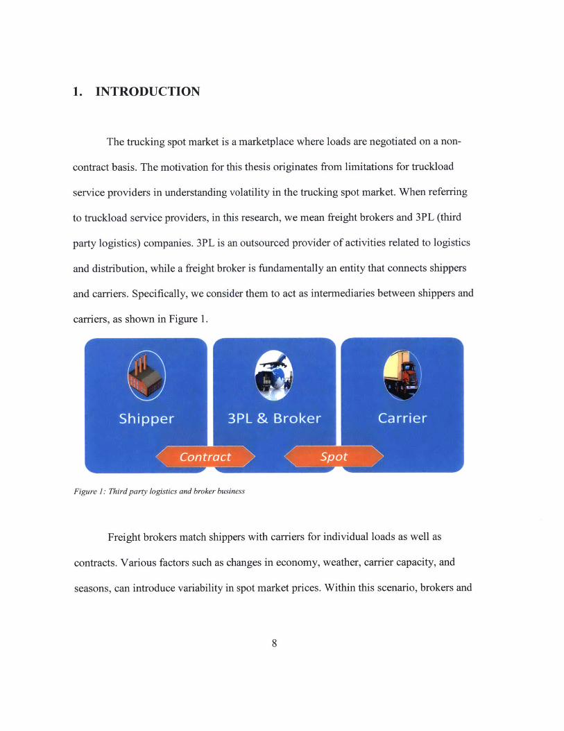
and carriers. Specifically, we consider them to act as intermediaries between shippers and
carriers, as shown in Figure 1.
Shipper 3PL &Broker Carrier
Contract Spot
Figure 1: Third party logistics and broker business
Freight brokers match shippers with carriers for individual loads as well as
contracts. Various factors such as changes in economy, weather, carrier capacity, and
seasons, can introduce variability in spot market prices. Within this scenario, brokers and
8
3PL companies need to develop a better understanding of the risk and the volatility
patterns of the spot market rates in order to mitigate market uncertainty.
Non-asset based logistics providers or brokers serve shippers that wish to
outsource some or all of their transportation needs, by negotiating rates with carriers and
manages day-to-day operations for their clients, effectively matching loads with carrier
availability and capacity. The difference between the cost of procuring carrier capacity
and the rate paid by the customer for the shipment is the margin that these firms earn on
the load.
To reduce risk, it is important for brokers and 3PLs to develop an understanding
of how the risk and the volatility patterns of the spot market rates are affected by
geography, season, and load distance, among others. In this thesis we develop and apply
methods for (i) assessing line-haul spot market risk, (ii) identifying factors impacting this
risk and (iii) pricing contracts for providing line-haul service on specific lanes. Measures
of volatility are defined and applied to key lanes to establish a risk profile. This risk
profile is then studied to determine the sources of volatility. Finally, we find the
distributions for the spot market prices of various lanes and show how these can used to
price the contracts. To initiate the research process, we first considered some important
questions:
1) What is volatility?
2) How does volatility impact non-asset does backed 3PL companies?
3) What factors influence spot market volatility?
9
4) How can non-asset backed 3PL company take advantage of, or mitigate impacts
of volatility?
5) How can be volatility and risk be measured and characterized?
The remainder of this thesis is organized as follows. Section 2 provides a
background of the trucking industry. Section 3 reviews the literature related to this topic.
Section 4 describes the tools, sources of information, and methods we used to collect,
treat and analyze the data, as well as describes the scenario presented in the dataset.
Section 5 shows the analysis performed through this research and the results obtained.
Finally, section 6 summarizes the insights and conclusion from this project, describing
the key findings and recommendations.
10
2. BACKGROUND
2.1. Trucking Industry
In the US, the major transportation mode is trucking. The industry transports
about nine billion tons and employed more than 1.3 million people in 2012. With a
market valued at $ 681.7 billion in 2013, the trucking business claimed about 81.2% of
the US commercial freight transportation market. S&P Capital IQ estimates that
aggregate revenues for the US commercial freight transportation market-including the
trucking, rail, air, water, and pipeline sectors-reached about $795.6 billion in 2012. As
comparison to these numbers, the US air freight was $ 78.8 billion industry in 2012, rail
freight $ 39.8 billion industry, water transportation $ 14.4 billion industry, while trucking
was $ 642.1 billion in the same year (S&P, 2014). In 2013 the overall transportation
sector was responsible for 9.3% of US GDP (US Department of Transportation - Bureau
of Transportation Statistics, 2014).
However, despite the sector's size, the trucking industry is a business with low
returns on capital, manpower and resources. This requires trucking companies to be more
and more efficient if they want to stay in business. In 2013, the seven leading truckload
carriers in US average 8.35% in operating margin, ranging from 2.9% to 13.6% (S&P,
2014). Within the trucking industry, freight transportation capacity has been facing
pressure from various sources in recent years in US. Many factors have been causing
capacity constraints and have been driving rates up. Some of those factors can be
predicted, but some cannot.
11
The trucking industry, involves a wide range of participants, including shippers,
carriers, brokers, and 3PLs. Of course there are more actors with different roles involved
in this huge industry (e.g. trucking associations, unions, etc.), but for the purpose of our
research we consider only the first four entities.
Another important distinction to be made in this market is between private fleets
and for-hire trucking segment. The first category relates to companies (shippers) that use
their own fleet to move their products, usually when the transportation plays a critical
role in achieving the company's goals. A good example of this case is retail stores, which
normally operate private fleets to facilitate efficient delivery of products to their stores. In
contrast, the for-hire trucking segment is the case when companies outsource their
transportation needs, contracting truckload providers to service them with transport. This
is the biggest segment of the trucking market, which involves either large motor carriers
and own operators, and the one we are going to focus in this research.
2.2. Shippers
Shippers are the central players in the trucking industry. They own the freight and
are the decision makers of who is going to move their loads. Shippers are the beneficial
owners of freight, and include manufacturers, distributors, and retailers (Sheffi, 2004).
They are entities (individual or companies) that have goods to be transported.
As mentioned before, shippers in the US can access truck capacity from either
their private fleets or for-hire trucking firms. Although little financial information is
available on private carriage, the ATA estimates that companies running their own
shipping operations provided services valued at some $292.0 billion in 2012, or about
12
45.5% of the trucking market, while the for-hire category generated revenues of $350.1
billion in the same year, or about 54.5% of the motor carrier business (S&P, 2014). For
example, one of the biggest private fleets in US is owned by Walmart, and they are also a
large buyer of for-hire TL services. In today's global economy, when dealing with for-
hire trucking, shippers may contract directly with the carriers, may hire third party
logistics providers or brokers to procure and manage their freight shipments, or use a mix
of both. Even when a company has their own fleet, in most cases, it will still need to
outsource a portion (inbound or outbound) of their operation to for-hire carriers or to
3PLs. It is uncommon to find shippers using only private fleets to run the entire business.
Walmart, for instance, uses its private fleet in parallel with for-hire trucking firms.
A shipper needs to balance the risks associated from transport of their goods. By
making the right decisions and choices, the shipper can dramatically improve the
competitiveness of the supply chain and the profitability of the company. The goal of any
shipper is to ensure the delivery of the freight to their customer in the right condition, at
the right time, at the right price, and in the most efficient way that optimizes the supply
chain as a whole.
2.3. Carriers
Freight transportation carriers provide the physical connection between shippers
and their customers (Sheffi, 2004). Carriers can be viewed as asset based companies,
which own most of the equipment (tractors and trailers) they use to provide transportation
services. They usually own or lease the trucks and directly employ the drivers.
Sometimes carriers are also called second party logistics (2PLs) from a shipper
13
standpoint. However, large motor carriers can also serve as brokers, as they use owner
operators or smaller carriers to move the loads under their responsibility. According to
the US Department of Transportation, in 2011, the US total number of interstate motor
carriers was 742,762.
We can divide TL carriers in four basic categories: international, national,
regional, and independent or owner operators. Independent operators are self-employed
commercial truck drivers that own and operate their own trucking business. They may
lease to a carrier or they may operate under their own authority.
Regarding the types of equipment, in the US trucking market, carriers can offer a
wide variety of trucks, which are differentiated by the type of trailers. The most common
types are: Dry Van, Refrigerated, Flatbeds, Liquid Tankers, Containers, Ragtops, and
others. There are also some specialized carriers that use specialized trailers as auto
carriers, bulk commodity, heavy haulers, cement mixer, dump truck, etc. In other
countries the types of trucks can vary from these, depending on culture, infrastructure,
regulations, and particular needs that may exist.
However, possibly the most important division of the for-hire trucking industry is
the truckload (TL), the less-than-truckload (LTL), and small package delivery (Parcel)
segments. Among the largest publicly traded companies in the TL business are
companies such as J.B. Hunt Transport Services Inc., Swift Transportation Co., Landstar
Systems Inc., and Werner Enterprises Inc. Representing the largest carriers in the LTL
business are Con-way Transport, and YRC Worldwide. UPS Freight and FedEx Freight
are the largest companies representing Parcel business, even though they do LTL and TL
in their operations (S&P, 2014).
As noted by Caplice (2007), truckload transportation firms (carriers) generally
handle shipments that are picked up at a location and driven directly to a single14
destination with no intermediate stops. This is contrasted with less-than-truckload (LTL)
or parcel shipments where the individual shipment might be picked up and transported to
an initial sorting hub on one vehicle and reloaded onto a separate vehicle for movement
to another terminal before finally being loaded onto another vehicle for final delivery
(Caplice, 2007).
Truckload (TL) carriers specialize in hauling large shipments for long distances.
In this segment, a truck will pick up a load from a shipper and carry it directly to the
destination, without transferring the freight from one equipment to another. The TL
market is highly fragmented without a single leading actor, mostly due to very low
barriers to new entrees. Less than truckload (LTL) carriers usually collect several
shipments of smaller sizes from different shippers in one truck that are going to similar
locations. The consolidation of freight requires a network of freight terminals. When the
shipment arrives at its destination terminal, the load is moved to a pickup-and-delivery
truck, and then transported to the final destination. Lastly, parcel carriers usually handle
small packages and freight that can be broken down into units less than 150 pounds. For
this research, we are analyzing data only from the TL market, limiting it to Dry Van
equipment into US territory.
2.4. 3PLs and Brokers
The terms "3PL" and "broker" are often used as interchangeable concepts in the
trucking industry. However, in reality, there are some differences between these two
terms. Although both entities act as intermediaries between shippers and carriers, their
roles can diverge a lot. A broker usually focuses on the execution of an individual
shipment, while a third-party logistics provider, in general, works more strategically.
15
Conceptually, brokers should refer to more basic services and 3PLs to more complex
operations.
Another common way to distinguish brokers and 3PLs is from an asset
standpoint. At large, brokers are non-asset-based providers, while modem 3PLs might
have at least some assets to back their operations. Nevertheless, most of the time, the
terms "3PL" and "broker" will overlap, as we can see 3PL companies acting as brokers
and vice versa.
We consider only freight brokers in this research. The first freight brokers started
in business selling the unused capacity of carriers in a particular region. As the
transportation industry developed, brokers began to help shippers to find carriers when
they needed transportation, and now it is not uncommon to have freight brokers entering
into long-term contracts with shippers to provide transportation on all of a shipper's lanes.
After agreed in a contract with the client, the broker then goes to the spot market obtain
truck capacity on an on-demand basis to supply transportation for the shipper.
The difference between the price the shipper pays to transport its goods and the
price the carrier charge to move the load is the profit the broker makes in this transaction.
Since the spot market rates are very volatile and the rates paid by shippers are agreed in
advance, the brokers' margin can vary widely, sometimes resulting even in a loss. With
that said, we can easily conclude that 3PLs and Brokers profitability derives from their
ability to forecast future spot market rates.
The broker's role can be defined as one of a matchmaker between carriers and
shippers, helping shippers that need to ship cargo find a trucking company that can
deliver the shipment on time and in good condition. The value of a broker is to facilitate a
business by bridging an operational or information gap. Brokers and 3PLs provide more
flexibility to shippers when the overall truck volume is low and volatile and available16
trucks are scarce, allowing them to access the trucking spot market without directly
participating of it. Brokers maintain relationships with thousands of carriers, and keep
track of their performance. Freight Brokers can normally deliver available capacity for
the right price.
2.5. Methods of Procurement of Truckload Transportation
Generally procurement is defined as the act of buying, purchasing or obtaining
goods or services from a supplier. In terms of truckload procurement, shippers procure
transportation using many different approaches. Some of them use a manual approach,
usually smaller shippers, while larger shippers are more likely to use systems to manage
procurement activities. Most large shippers buy transportation services using requests for
proposals (RFPs), leading to contract prices that are typically in effect for one to two
years (Sheffi, 2004).
Currently, a wide variety of different electronic market formats can be used for
procurement in the truckload industry, including combinatorial auctions, private and
public exchanges, and electronic catalogs (Caplice, 2007). The next step after the
implementation of one of these tools is to establish the rates for each lane that will be
serviced by the carrier for a certain period of time. These rates will be used on the
execution stage on a daily basis every time the carrier moves a load for the shipper.
However, besides formal contracts between shipper and carriers, there is also an
alternative for shippers to procure truckload transportation, which is accessing the freight
spot market. A spot transaction happens usually for a single load and the price is
determined by the market only at the time when the load needed to be moved. In the next
17
section we are going to emphasize specifically the trucking spot market, since its
understanding is crucial for the comprehension of our research.
2.6. Trucking Spot Market
The trucking spot market is composed of two main players, regular carriers (small
and large) and owner operators. Owner operators usually haul as free-lancers, going to
the load that fits better their needs. However, in the carrier's case, their role in the spot
market is a little bit different. After completion of a load, they need to relocate their
equipment to be ready to serve another customer they made commitments to. This makes
many carriers willing to sell their extra capacity below market price to return to their
original base. Sometimes carriers can lower their service rates down to the marginal cost
of service for trips that have to be performed whether or not they carry a load (Garrido,
2007).
The spot market is a common term for single transactions where the price is
determined near (or at) the time when the shipper needs extra capacity to move its goods
(Bignell, 2013). Due to this logic, the spot market prices can be substantially lower or
higher than average market prices, since this market reflects exactly the current
transportation capacity and demand.
One method that shippers use is to contract 3PL or freight broker companies in
order to access a large number of carriers and to have more flexible capacity. A spot
market transaction begins with a negotiation between the shipper and the broker to agree
on a rate for a particular lane, followed by the negotiation between the broker and the
carriers it has in its network of contacts (Bignell, 2013). When the broker agrees on price
18
with a carrier (or owner operator), the transaction is closed and the load can be moved.
The difference between the rate agreed with the shipper and the rate negotiated with the
carrier is the margin the broker makes in that particular transaction. Companies such as
C.H. Robinson, Total Quality logistics, XPO Logistics, and Coyote Logistics are among
the largest brokerage firms in US and North America.
These days, it is very common to have 3PL and broker companies entering the
auction process competing with regular carriers, In this case, brokers provide long-term
rates for some lanes in order to get annual contracts with the shipper. This is the case of
our sponsor (ABC Company), which has many contracts set with shippers, but, as a non-
asset based logistics provider, needs to rely in the truck spot market to physically provide
the service. Brokerage business logic relies on believing that the aggregate amount that
they pay to carriers over the course of the contract will be less than the aggregate revenue
received from the shipper. Their success depends on the capability to guess future spot
market rates.
For the reasons stated above and many other factors that constrain trucking
capacity, the trucking spot market rates are far more volatile than contract rates.
According to the DAT Truckload Report (2014), spot market rates exceeded contract
rates on 45% of hauls from mid-April to mid-May in 2014. In previous years, between
20% and 25% of spot market rates were higher than contract rates (Thornton, 2014). As
we mentioned, this scenario can be influenced by many factors. Regions of origin and
destination, types of loads, likelihood of backhaul, total distance and deadhead distance,
load and unload time, load weight, and others are always a concern for carriers and owner
operators when choosing which load to accept. Likewise, the type of trailer required and
specific requirements for the load are also constraints.
19
There are also hidden factors that play a role in rates' volatility, which will be
identified later when analyzing the data on this paper. The most common are: geographic
factors, such as seasonality (Christmas, agricultural harvest, etc.); different types of
equipment; general economic indicators (e.g. in growing economies GDP puts a pressure
on truck availability); government policy (e.g. truck driver hours-or-service regulation
changes); load and unload time; week day; manpower capacity; and others.
20
3. LITERATURE REVIEW
3.1. Introduction: Opportunity for Improved Profitability
Although no substantial research has been done on this specific topic, some
previous work has addressed related topics involving the spot market of the transportation
industry. Third-party-logistics (3PL) providers connect shippers with carriers by
matching loads with truck capacity. The difference between the cost of procuring truck
capacity and the price paid by the shipper for the shipment is the margin the 3PL
company earns on a load. The price charged to the shipper is generally agreed upon in
advance via an annual contract. In contrast the truck capacity is obtained from the spot
market within a week of the scheduled load pickup time.
Bignell (2013) explores the importance of utilizing trucking spot market rate
information and knowledge to improve contract formulation and negotiation. Because
rates with shippers are established prior to negotiations with carriers, the margin achieved
by a broker on any particular transaction can vary widely and may even be negative,
depending on general economic conditions, market trends, and seasonal variations.
In addition, Bignell (2013) also establishes that spot market behavior varies
geographically and with respect to time. This thesis explores a better understanding of the
spot market volatility patterns across the various markets. Very limited research has been
conducted thus far in the scientific community to gain an in-depth knowledge of volatility
in truckload spot market prices. Such research has been performed for spot electricity
market, airline tickets and commodities such as silver and fuel.
21
By acknowledging this gap in literature, our final objective is to identify and
quantify individual patterns of volatility in the spot market, and based on that, to produce
a data-driven model that allows freight brokers and 3PL companies to assess and reduce
their risk. This knowledge can be utilized to enhance existing contracting models with
carriers to reduce risk. Since there is very limited research specific to a truckload spot
market on this topic, other types of spot markets are also within scope as the findings
from those markets may be closely applicable to the truckload spot market. The literature
review focuses on the following topics: price volatility in spot market; factors
contributing to price volatility in spot market; volatility patterns with respect to time and
location; and mathematical analysis.
3.2. Price Volatility in Spot Market
Price volatility in spot market transactions is a popular topic of study among
researchers in the commodities and financial markets. Over the years, researchers have
studied the price volatility of a variety of items including financial instruments such as
stocks and commodities such as silver, electricity and fuel. In the research conducted by
Simonsen on volatility of power markets, volatility is defined as a characteristic to
measure the fluctuations or risk associated with purchasing (Simonsen, 2005).
In a separate study conducted by Gillen and Mantin on price volatility in the
airline markets, volatility is defined as the level of uncertainty associated with the erratic
change of the value of an item over time (Gillen & Mantin, 2009). Simply put, this
measure is utilized to answer how well and the degree of certainty with which one can
predict the change in the price of an item. Standard deviation of the price is the
22
descriptive statistic that is proposed to be utilized to measure the volatility in that case.
Further, it is suggested by Gillen & Martin that volatility indicates the overall instability
and deviation of the demand relative to the general expectation for a good or service.
Therefore, volatility of the prices may in reality indicate that the demand itself is
volatile. The instability and volatility in prices is seen as a significant factor in customer's
future expectations of prices and relevant decisions. In the financial industry, volatility is
a measure that is utilized to quantify the risk associated with a financial instrument. A
common volatility measure in the financial sector includes the Chicago Board of Options
Exchange (CBOE) Volatility Index (VIX) which measures the volatility of the S&P 500
and is known to measure the volatility of the index. Other applications of volatility
models suggested by Simonsen include the foreign exchange market as well as the
volatility associated with the inflation of an economy (Simonsen, 2005). Exponential
smoothing approach is also investigated due to its simplicity. In the case of the electricity
model, volatility is seen as an important and useful input into models that forecast the
prices in electricity markets. Conceptually the same approach can be applied to the carrier
transaction data to improve the contract and the pricing strategy between the shipper and
the carrier.
3.3. Factors Contributing to Price Volatility in Spot Market
According to Cassidy, the spot market for truckloads is quite close to the market
equilibrium (Cassidy, 2010). Carrier executives believe that the volatility, uncertainty and
imbalance is caused as a result of various factors such as shortage of truck drivers, rising
and fluctuating fuel costs and increasingly constrained regulatory environment. In the
23
same line of reasoning, Thornton emphasizes that the responsible for higher rates in the
trucking market are factors that constrain capacity, including more stringent regulations,
extreme weather, increasing operating costs, and a chronic shortage of experienced
drivers (Thornton, 2014). As mentioned previously, the freight transportation market has
been facing many ups and downs in the last two or three years, causing freight brokerage
business to become more risky as this volatility is poorly understood by the main players.
Particularly, the rising fuel prices negatively impact smaller carriers with older
trucks who do not have much leverage in negotiating spot market prices and recovering
fuel surcharges. On the other hand larger carriers have greater power in price negotiations
and are equipped with newer and more fuel efficient trucks. In the case of fuel prices,
large and erratic fluctuations may occur due to several different reasons ranging from
geopolitical unrest in oil producing nations to refinery capacity constraints and weather
disruptions. Furthermore, the government has made efforts to improve the drivers'
conditions by proposing to introduce more mandatory breaks, reduce the driving time per
day and equip trucks with monitoring and safety devices. As per industry experts these
changes can directly increase the cost to the carrier thereby increasing the overall
volatility and baseline for the trucking spot market prices. In the case of the research
conducted on the airlines industry by Gillen and Mantin, market share i.e. the number of
planes is seen as a factor that influences the volatility (Gillen & Mantin, 2009). A
dummy variable is introduced in the regression model to indicate whether or not the
market share for a single carrier is more than 90%. In addition, other factors that were
identified by Gillen and Mantin include the presence of a low cost carrier in the route
being taken by the company, the total distance of the lane and whether or not the journey
is non-stop.
24
3.4. Volatility Patterns
Simonsen observes the phenomenon of volatility clustering in spot markets
whereby the volatility of prices is intermittent with periods of high volatility followed by
less volatile periods. Simonsen further investigates the relationship between volatility and
time by examining the temporal volatility-volatility correction function to quantify the
concept. In addition, he observes that prices are particularly more volatile in the summer
months than rest of the year, thus illustrating the time-dependent nature of volatility
(Simonsen, 2005).
Volatility also varies with respect to price levels. At low price levels of spot
prices, there is a stronger relationship between volatility and price levels i.e. volatility
increases with an increase in price. On the other hand, at high price levels, there is a weak
relationship between volatility and price levels. While our research focuses on the spot
market price volatility of truckloads, the volatility patterns observed in other markets
such as commodities and financial instruments will offer fresh insights and creativity.
Similarly, Gillen and Mantin investigate how volatility changes with respect to time in
the airlines market. It was done by plotting and studying the change in volatility with
respect to time across the different geographies (Gillen & Mantin, 2009). Volatility
drastically increases during the last 2 weeks of the month though the average price level
may not necessarily increase or decrease, thereby confirming the time dependent nature
of volatility.
25
3.5. Mathematical Analysis
A mathematical technique commonly used in the volatility analysis of the prices
in the various spot markets is regression analysis. For example, in the spot market for
airline tickets, Gillen and Mantin performed regression analysis to identify the underlying
determinants of price volatility (Gillen & Mantin, 2009). In order to do this, market
structure variables were formulated to represent the market concentration (Hirschman-
Herfindahl Index), market domination and whether or not an airline was low cost. In
addition, a distance variable was included to represent the route characteristics. By
simulating the regression models with the various explanatory variables and examining
the R 2 values generated, Gillen and Martin were able to determine whether or not each of
the factors had any influence on the volatility of the prices (Gillen & Mantin, 2009). In
the specific example, it was determined that the presence of a low cost carrier on a
specific route does not impact the price volatility.
When modeling the volatility of railway freight in China, Dai, Sriboonchitta and
Li (2012) used symmetric and asymmetric conditional volatility models (GARCH, GJR-
GARCH and EGARCH) in order to estimate the volatility in monthly railway freight
volume. According to their results, it indicated that the volatility has an asymmetric effect
on risk from positive and negative shocks of equal magnitude.
In addition to the transportation field, we also considered options in different
fields with similar behaviors. One option that makes sense for us is the finance market. In
finance, the risk of stocks and options is calculated by using the stock prices' volatility.
By testing the significance of beta, stock riskiness is predicted (Bahhouth, Maysami and
Khoueiri, 2010). To determine an option price risk in units of stock price risk is relevant
26
for hedging, risk management, asset pricing and performance measurement (Branger and
Schlag, 2007). This approach is in some way analogous to the 3PL companies acting in
the trucking spot market, in which they have to "bet in" a rate while setting contracts with
shippers and later they have to buy transportation capacity in the spot market.
3.6. Conclusion: Cross Industry Insights
The trucking industry in US provides an essential service to the US economy by
transporting large quantities of raw materials, works in process, and finished goods over
the country. In the past three years, 3PL enterprises were struggling to predict future
trucking spot rates. In our research, we will try to fill this gap when understanding the
volatility that exist in this specific market, making it easier to be explored. We will focus
on understanding the spot trucking market behavior to posteriorly create a feasible model
able to enhance the spot rates forecasting process. 3PL providers will benefit from a
better understanding of rate volatility and able to increase their business' profitability.
It is evident through the literary review that there is very limited knowledge
regarding the spot market price volatility in the freight transportation and truckload
industry. It is recommended to adopt some techniques and methodologies utilized in
other industries and apply them specifically to the truckload spot market price volatility
scenario to develop an in-depth understanding of truckload spot market price volatility.
27
4. METHODOLOGY AND DATASET
In this section, we describe the tools, sources of information, and methods we
used to collect, treat and analyze the data. We also will describe the scenario presented in
the dataset.
4.1. The Dataset
The original data were provided by our sponsor company's strategic team, which
were extracted from the company's system. The dataset includes shipment records of dry
van equipment, nationwide (US) over the past three years (From October 2011 through
September 2014). The data are composed of 1,609,594 rows of load shipments during
this three years period. Each row of data indicates a load shipment by a carrier to a
shipper and consists of the attributes shown in table 1.
28
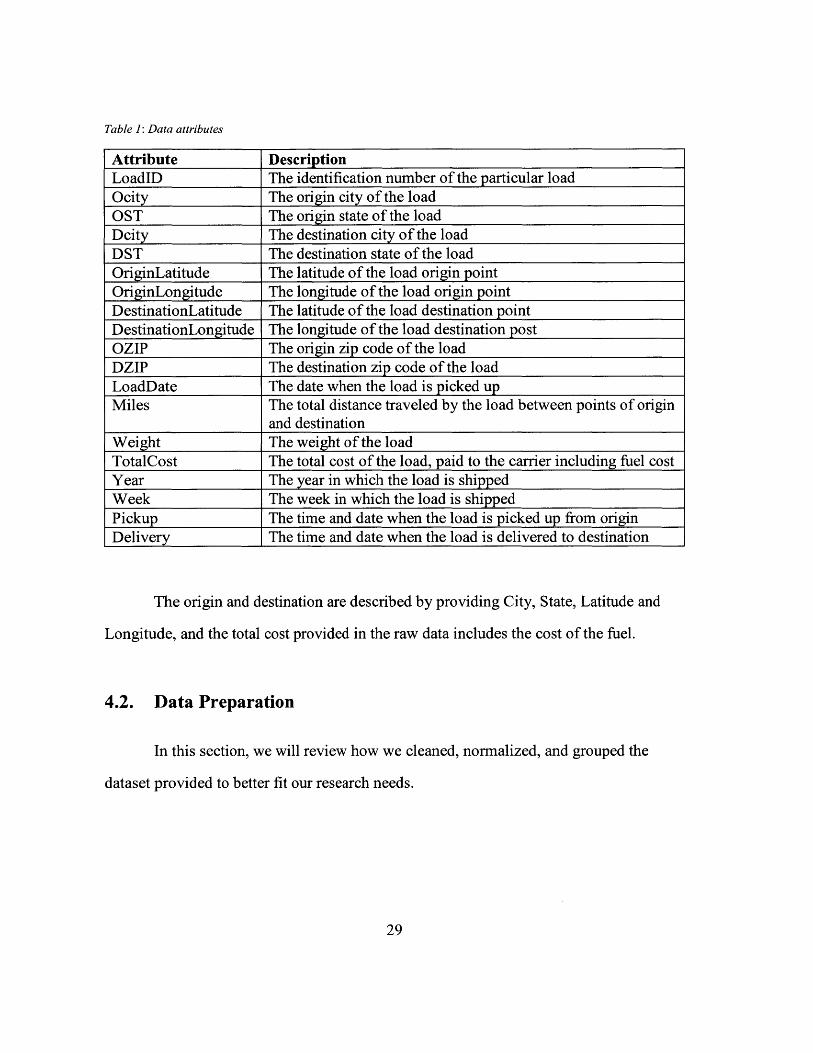
Table 1: Data attributes
Attribute DescriptionLoadID The identification number of the particular loadOcity The origin city of the loadOST The origin state of the loadDcity The destination city of the loadDST The destination state of the loadOriginLatitude The latitude of the load origin pointOriginLongitude The longitude of the load origin pointDestinationLatitude The latitude of the load destination pointDestinationLongitude The longitude of the load destination postOZIP The origin zip code of the loadDZIP The destination zip code of the loadLoadDate The date when the load is picked upMiles The total distance traveled by the load between points of origin
and destinationWeight The weight of the loadTotalCost The total cost of the load, paid to the carrier including fuel costYear The year in which the load is shippedWeek The week in which the load is shippedPickup The time and date when the load is picked up from originDelivery The time and date when the load is delivered to destination
The origin and destination are described by providing City, State, Latitude and
Longitude, and the total cost provided in the raw data includes the cost of the fuel.
4.2. Data Preparation
In this section, we will review how we cleaned, normalized, and grouped the
dataset provided to better fit our research needs.
29
4.2.1. Data Cleaning
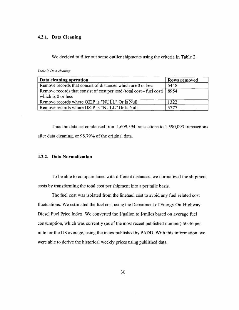
We decided to filter out some outlier shipments using the criteria in Table 2.
Table 2: Data cleaning
Data cleaning operation Rows removedRemove records that consist of distances which are 0 or less 5448Remove records that consist of cost per load (total cost - fuel cost) 8954which is 0 or lessRemove records where OZIP is "NULL" Or Is Null 1322Remove records where DZIP is "NULL" Or Is Null 3777
Thus the data set condensed from 1,609,594 transactions to
after data cleaning, or 98.79% of the original data.
1,590,093 transactions
4.2.2. Data Normalization
To be able to compare lanes with different distances, we normalized the shipment
costs by transforming the total cost per shipment into a per mile basis.
The fuel cost was isolated from the linehaul cost to avoid any fuel related cost
fluctuations. We estimated the fuel cost using the Department of Energy On-Highway
Diesel Fuel Price Index. We converted the $/gallon to $/miles based on average fuel
consumption, which was currently (as of the most recent published number) $0.46 per
mile for the US average, using the index published by PADD. With this information, we
were able to derive the historical weekly prices using published data.
30
4.2.3. Data Aggregation and Selection
We aggregated and selected the data for analysis purposes. On top of the
segmentation we decided to aggregate the data in terms of lanes origin and lanes
destination. The data was aggregated in lanes by 3 digit origin and destination zip codes
to improve significance and relevance. This resulted in an aggregated data set consisting
of 1,164,953 spot transactions.
Each transaction consists of Load Date, Origin and Destination State and 3-digit
ZIP, Cost per load without fuel (Average, Minimum and Maximum), Distance (Average,
Minimum and Maximum), Cost per mile and Load Count. Load count indicated the
number of loads in a particular 3-digit to 3-digit lane. The average, minimum and
maximum costs and distances are calculated using the information for a 3-digit to 3-digit
lane for a particular day.
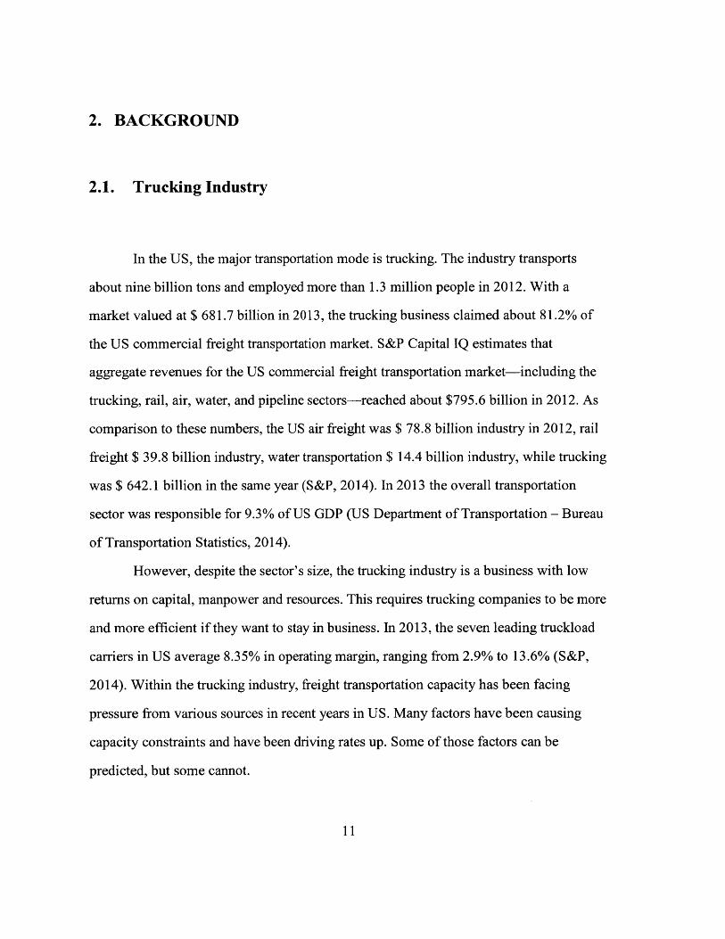
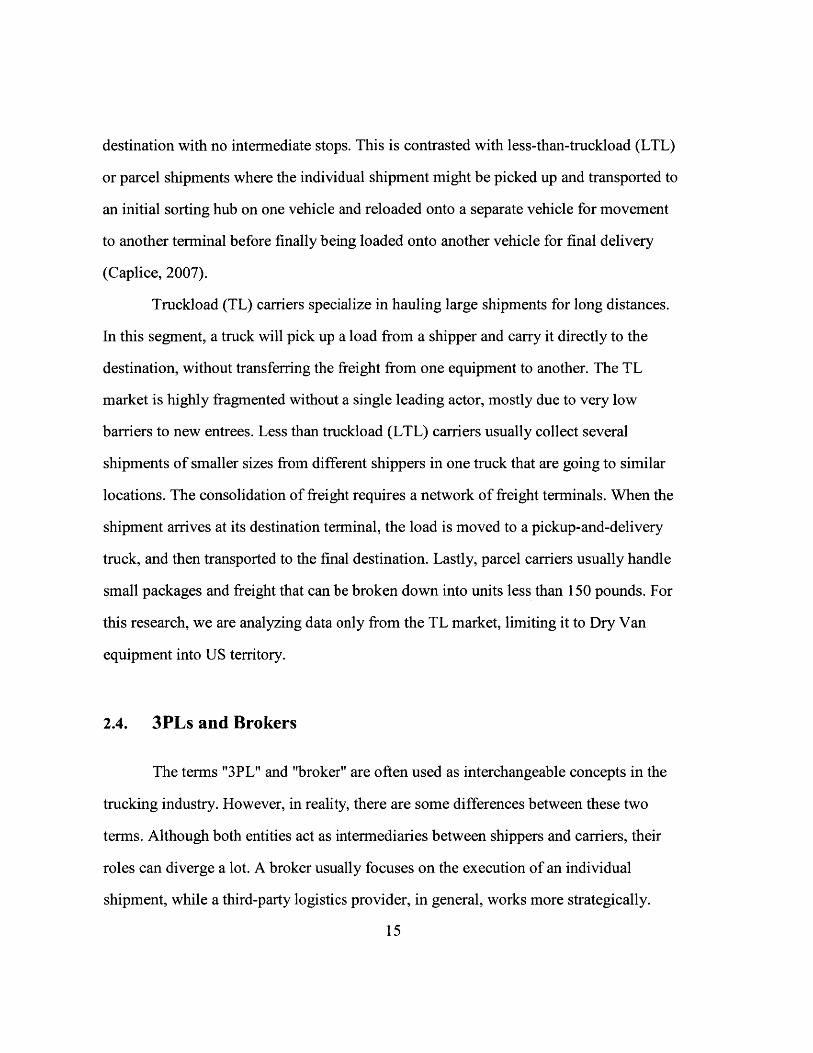
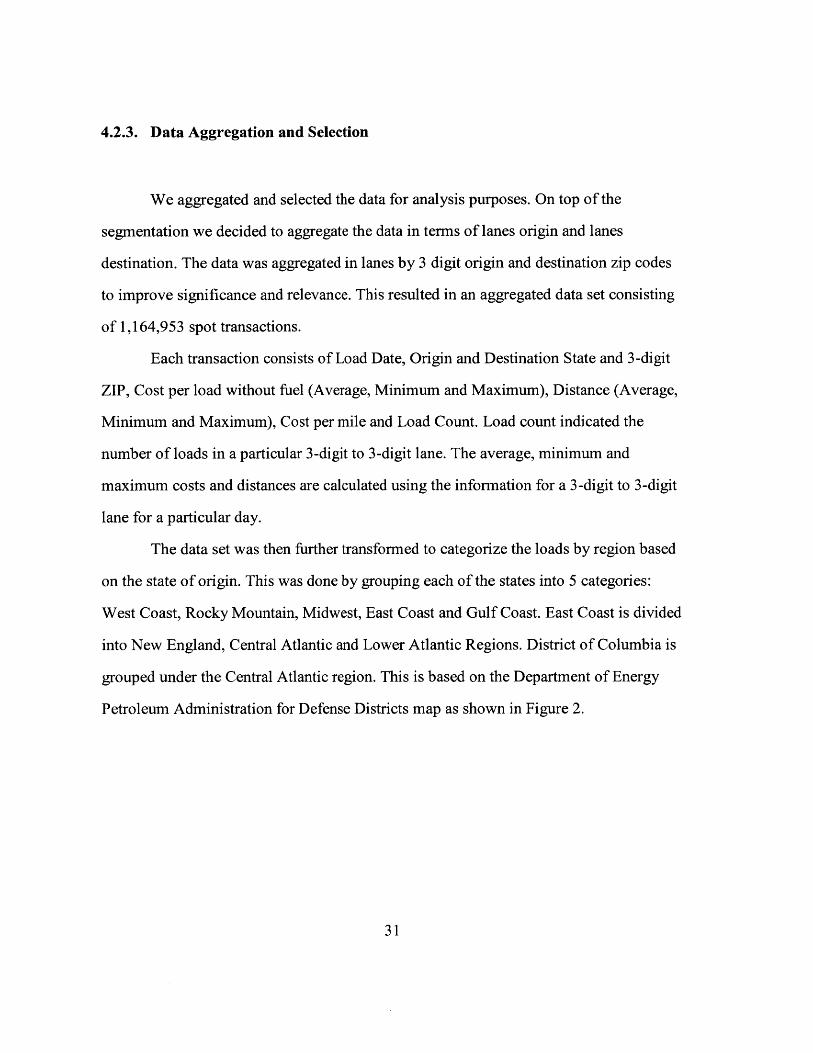
The data set was then further transformed to categorize the loads by region based
on the state of origin. This was done by grouping each of the states into 5 categories:
West Coast, Rocky Mountain, Midwest, East Coast and Gulf Coast. East Coast is divided
into New England, Central Atlantic and Lower Atlantic Regions. District of Columbia is
grouped under the Central Atlantic region. This is based on the Department of Energy
Petroleum Administration for Defense Districts map as shown in Figure 2.
31
Petroleum Administration for Defense Districts
OR PADD 2:PADD 6: Midwest
West Coast, 'A-
AK, HI .1 *
C T"
AZ
PAOOIA
PADD 1:EastCoast
Figure 2: Petroleum administration for defense districts map
4.3. Measures of Volatility
Three measures of volatility were utilized to quantify the volatility and to
characterize the risk: Coefficient of variation (CV), beta (p) and average month/month
percentage change (AMoM).
4.3.1. Coefficient of variation
The coefficient of variation (CV) is a standardized measure of dispersion of a
frequency distribution. It is defined as the ratio of the standard deviation to the mean. The
coefficient of variation is useful because the standard deviation of data must always be
understood in the context of the mean of the data. In contrast, the actual value of the CV
32

is independent of the unit in which the measurement has been taken, so it is a
dimensionless number. CV is calculated as:
CV=
Here a is the standard deviation of the linehaul cost per mile and i is the average
of the linehaul cost per mile. The CV is calculated based on the monthly values of -and
p during 2012 and 2013.
4.3.2. Beta
The Beta value is utilized to indicate the relative risk of a lane in comparison to an
index such as the national index or the CASS index. Beta is calculated as:
Cov(x, y) (2)
Var(y)
Here x is the cost per mile values of a lane and y is the cost per mile values of an
index within a time period. To calculate a 8 value for a time period, the average monthly
values are utilized within the time period. The values for the beta for a given region or
lane can be interpreted as described in the Table 3 below. The time intervals used for the
beta calculations can be quarter to quarter or yearly.
33
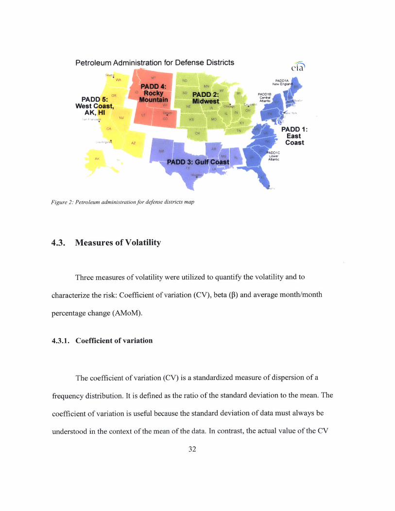
Table 3: Beta value interpretation
Beta Value InterpretationP<0 Regional index moves in the opposite direction as compared to the
national indexp=0 Regional index is uncorrelated to the national index0<P<1 Regional index moves in the same direction as the national index but is
less volatile=1 Regional index moves in the same direction as the national index and
by the same amount>1 Regional index moves in the same direction as the national index and is
more volatile
The reliability of the beta values is calculated using Pearson's product-moment
correlation coefficient (R-Squared value). This measures the linear correlation
(dependence) between two variables giving a value between +1 and -1. 1 indicates total
positive correlation, 0 indicates no correlation and -1 indicates total negative correlation.
4.3.3. Average month/month percentage change
As the third measure, volatility is calculated by examining the average month over
month percentage change in the cost per mile rates based on the average monthly rates for
each region. This indicates the extent to which the cost per mile rate varies on a monthly
basis. It is calculated as:
E[Mn) * 100%]Avg= n
n
(3)
Here Mn indicates the average monthly cost per mile rate for month n and Mn_ 1
indicates the average monthly cost per mile rate for month n - 1.
34
4.4. Lane Characterization
A subset of data of 3digit-3digit zip code, which have at least 1 load per month
every month for 2012 and 2013 are utilized to more closely analyze and understand the
characteristics of individual lanes. In total when aggregating the data by month, there are
90,275 unique 3digit origin to 3digit destination zip code lanes. Once this data is filtered
out to include only lanes which have at least 1 load per month every month for 2012 and
2013, the number of lanes is reduced to 674. If the zip code 3 digit zip code lanes are
filtered out to include only lanes which have at least 1 load per week every week for 2012
and 2013, the number of lanes is reduced to 30. On average, the national linehaul cost per
mile changes by 0.41% week over week during 2012 and 2013 and 1.51% month over
month. The coefficient of variation are 0.08 and 0.09 monthly and weekly respectively.
Hence monthly values were utilized to ensure a sufficiently large data set across the
various regions. However, weekly analysis is conducted on the Laredo to Houston (780-
770) lane in the Management Implementation section of the thesis. The lanes are then
characterized by volatility and risk based on the Beta value for 2012 and 2013 against
the national index as well as the coefficient of variation and average monthly percentage
change for 2012 and 2013.
35
4.5. Factors Related to Volatility
The relationships between volatility, distance and volume are investigated.
Volatility is examined using both beta and the coefficient of variation. First, the
relationship between coefficient of variation and beta is examined to ensure that both the
measures are relevant.
4.6. Linear Regression
Using the monthly average cost per mile in years 2012 and 2013 for each region
(Central Atlantic, Lower Atlantic, New England, Gulf Coast, West Coast, Mid-West, and
Rocky Mountain) as the dependent variable, and interchanging some independent
variables, such as GDP Index, date (month and year), number of trucks at origin, and
commodities seasons (agricultural activity), several regression analysis were performed
to test which factors influence or do not influence the spot market rates in a given region.
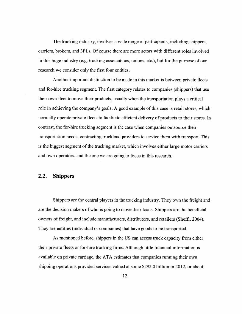
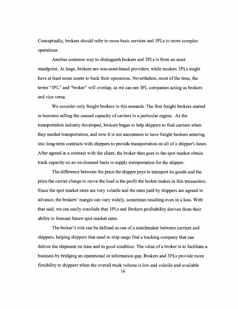
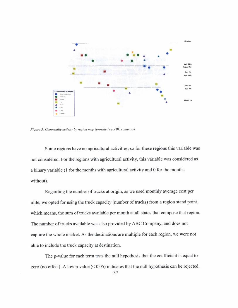
Figure 3 shows the commodity map used to account for the crops' seasons by
regions, which was provided and developed by our thesis sponsor (ABC Company),
based on their empirical analysis over the years.
36
U. .
without).~t
e, pJef s 1k
lo JWm lot
A* -1
A "WOO, lot
A
A
Figure 3: Commodiy activity by region map (provided by ABC company)
Some regions have no agricultural activities, so for these regions this variable was
not considered. For the regions with agricultural activity, this variable was considered as
a binary variable (1 for the months with agricultural activity and 0 for the months
without).
Regarding the number of trucks at origin, as we used monthly average cost per
mile, we opted for using the truck capacity (number of trucks) from a region stand point,
which means, the sum of trucks available per month at all states that compose that region.
The number of trucks available was also provided by ABC Company, and does not
capture the whole market. As the destinations are multiple for each region, we were not
able to include the truck capacity at destination.
The p-value for each term tests the null hypothesis that the coefficient is equal to
zero (no effect). A low p-value (< 0.05) indicates that the null hypothesis can be rejected.37

In other words, a predictor that has a low p-value is likely to be a meaningful addition to
your model because changes in the predictor's value are related to changes in the response
variable. Conversely, a larger (insignificant) p-value suggests that changes in the
predictor are not associated with changes in the response.
4.7. Chapter summary
In this section we outlined the steps taken before analyzing the data and the tools
we utilized to perform the analysis. We started with 1,609,594 rows of load shipments
and ended up with 1,164,953 rows of data, which were later grouped in 7 different
regions. The next chapter will discuss in more details the analyses performed on the
resulted data and the results obtained through this process.
38
5. RESULTS
5.1. Data Exploration
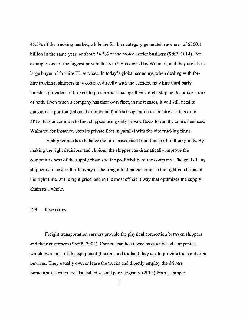
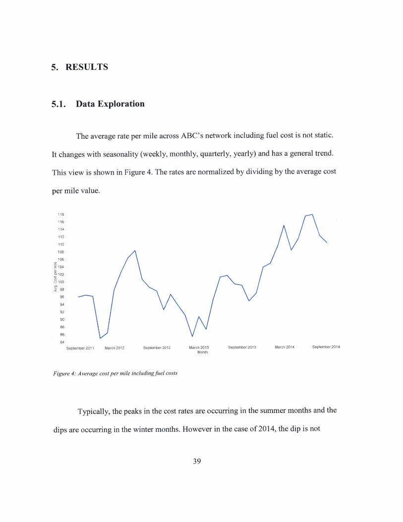
The average rate per mile across ABC's network including fuel cost is not static.
It changes with seasonality (weekly, monthly, quarterly, yearly) and has a general trend.
This view is shown in Figure 4. The rates are normalized by dividing by the average cost
per mile value.
118
116
114
112
110
108
106
104
a 102
0 100
< 98
96
94
92
90
88
86
84
September 2011 March 2012 September 2012 March 2013 September 2013 March 2014 September 2014Month
Figure 4: Average cost per mile including fuel costs
Typically, the peaks in the cost rates are occurring in the summer months and the
dips are occurring in the winter months. However in the case of 2014, the dip is not
39
prominent in the winter months likely due to harsh nation-wide weather conditions which
put a pressure on the trucking industry, causing the rates to increase.
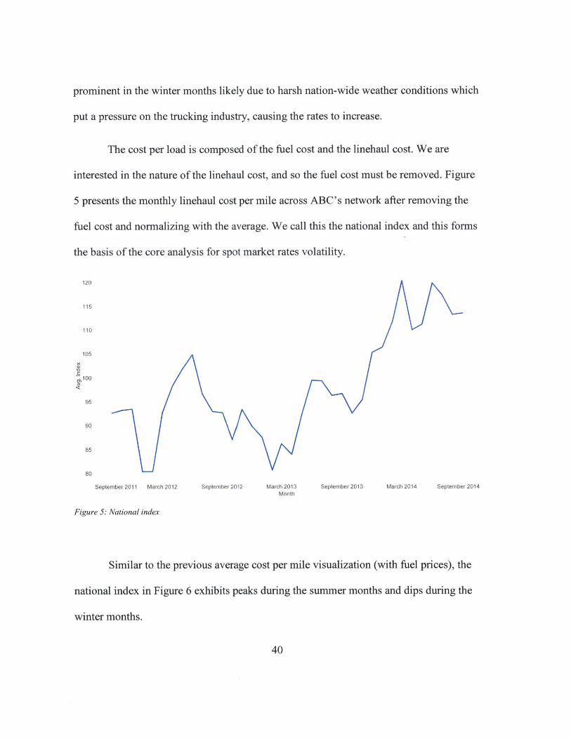
The cost per load is composed of the fuel cost and the linehaul cost. We are
interested in the nature of the linehaul cost, and so the fuel cost must be removed. Figure
5 presents the monthly linehaul cost per mile across ABC's network after removing the
fuel cost and normalizing with the average. We call this the national index and this forms
the basis of the core analysis for spot market rates volatility.
120
115
110
105
100
95
90
85
80
September 2011 March 2012 September 2012 March 2013 September 2013 March 2014 September 2014Month
Figure 5: National index
Similar to the previous average cost per mile visualization (with fuel prices), the
national index in Figure 6 exhibits peaks during the summer months and dips during the
winter months.
40
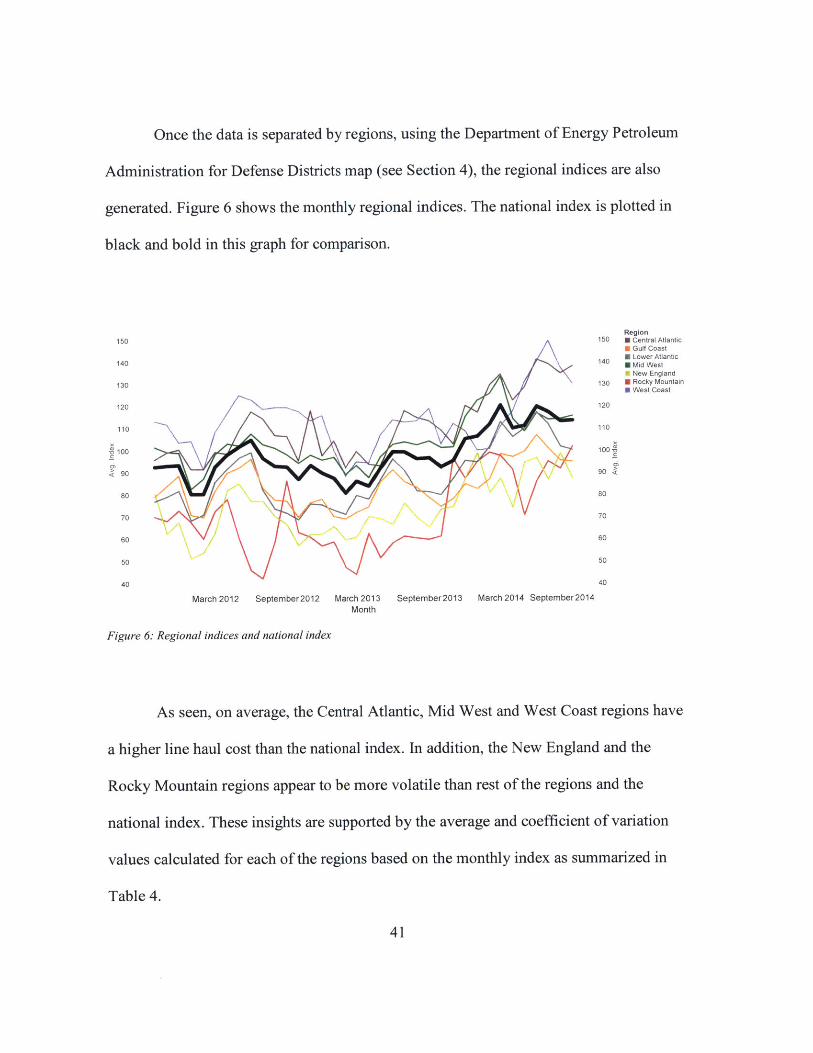
Once the data is separated by regions, using the Department of Energy Petroleum
Administration for Defense Districts map (see Section 4), the regional indices are also
generated. Figure 6 shows the monthly regional indices. The national index is plotted in
black and bold in this graph for comparison.
Region150 150 Central Atlantic
: Gulf Coast
140 140 Lower Atlantic
1 14 0 Mid WestNew England
130 130 N Rocky MountainU West Coast
120 120
110 110
-o 100 100
<90 90 <
80 80
70 70
60 60
50 50
40 40
March 2012 September 2012 March 2013 September2013 March 2014 September 2014Month
Figure 6: Regional indices and national index
As seen, on average, the Central Atlantic, Mid West and West Coast regions have
a higher line haul cost than the national index. In addition, the New England and the
Rocky Mountain regions appear to be more volatile than rest of the regions and the
national index. These insights are supported by the average and coefficient of variation
values calculated for each of the regions based on the monthly index as summarized in
Table 4.
41
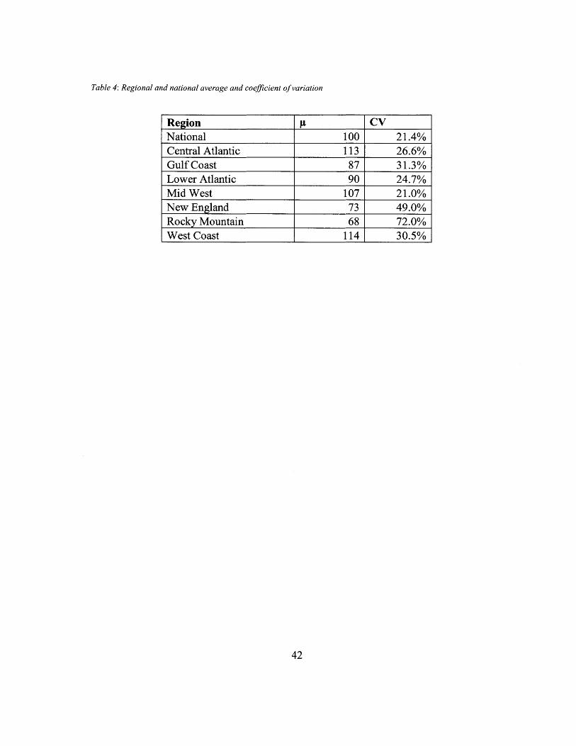
Table 4: Regional and national average and coefficient of variation
Region Ft CVNational 100 21.4%Central Atlantic 113 26.6%Gulf Coast 87 31.3%Lower Atlantic 90 24.7%Mid West 107 21.0%New England 73 49.0%Rocky Mountain 68 72.0%West Coast 114 30.5%
42
5.2. Distribution of Linehaul Cost per Mile
The historical cost per mile values of the national index are examined to
determine an appropriate distribution fit. The probability distribution function is then
utilized to determine the contract price that ABC should charge the shipper given that
ABC would like to earn a margin of m dollars with a probability of p. If C is the cost per
mile on a given lane and m is the desired margin with a probability of p, the contract
price x can be determined as (i.e. x - c >= m) by solving the below equation:
P(C <= x - m) = p (4)
The distributions for the different regions are outlined in Table 5 and are visualized in
Figure 8.
43
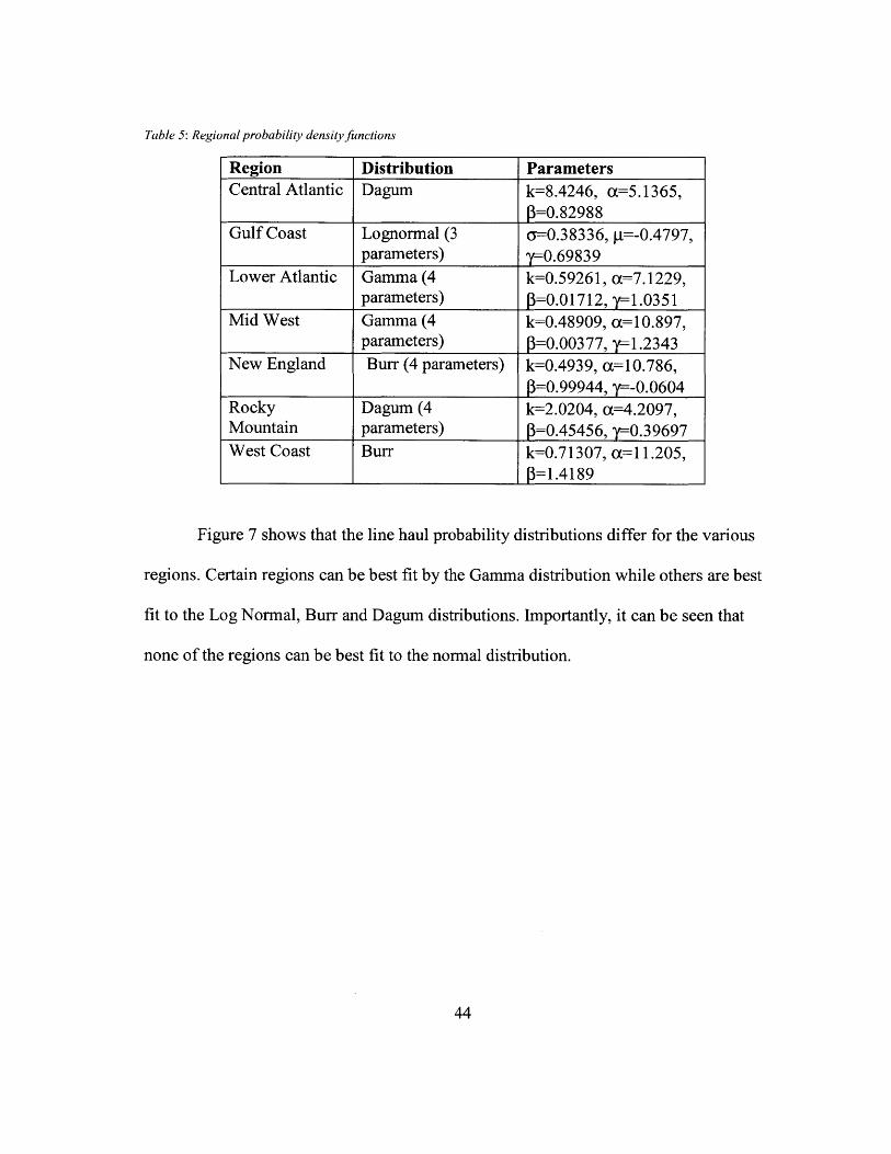
Table 5: Regional probability density functions
Region Distribution ParametersCentral Atlantic Dagum k=8.4246, cx=5.1365,
=0.82988Gulf Coast Lognormal (3 cy=0.38336, p=-0.4797,
parameters) y=0.69839Lower Atlantic Gamma (4 k=0.59261, cx=7.1229,
parameters) p=0.01712, -1.0351Mid West Gamma (4 k=0.48909, x=10.897,
parameters) pl=0.00377, y=.2343New England Burr (4 parameters) k=0.4939, a=10.786,
=0.99944, y=-0.0604Rocky Dagum (4 k=2.0204, a=4.2097,Mountain parameters) P=0.45456, 7-0.39697West Coast Burr k=0.71307, o=1l1.205,
=1.4189
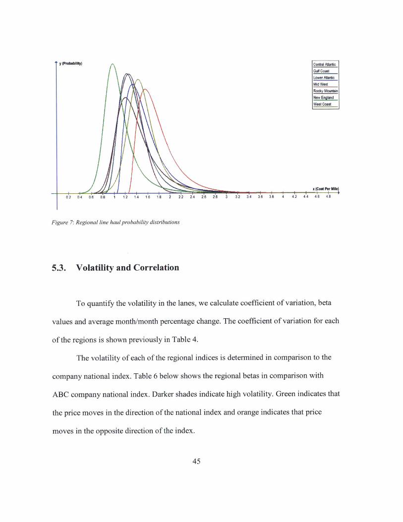
Figure 7 shows that the line haul probability distributions differ for the various
regions. Certain regions can be best fit by the Gamma distribution while others are best
fit to the Log Normal, Burr and Dagum distributions. Importantly, it can be seen that
none of the regions can be best fit to the normal distribution.
44
y (Probability) Central Atantic
Gulf Coast
Lower Atlantic
Mid West
Rocky Mountain
New EnglandWest Coast
x (Cost Per Mile)
0'2 04 06 0.8 1 12 14 1,6 18 2 2.2 2.4 2.6 2.8 3 3.2 3.4 3.6 3.8 4 42 4.4 4.6 4.8
Figure 7: Regional line haul probability distributions
5.3. Volatility and Correlation
To quantify the volatility in the lanes, we calculate coefficient of variation, beta
values and average month/month percentage change. The coefficient of variation for each
of the regions is shown previously in Table 4.
The volatility of each of the regional indices is determined in comparison to the
company national index. Table 6 below shows the regional betas in comparison with
ABC company national index. Darker shades indicate high volatility. Green indicates that
the price moves in the direction of the national index and orange indicates that price
moves in the opposite direction of the index.
45
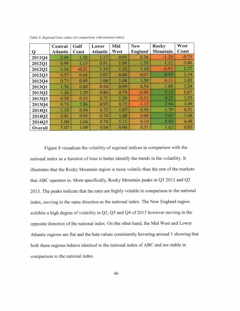
Table 6: Regional beta values (in comparison with national index)
Central Gulf Lower Mid New Rocky WestQ Atlantic Coast Atlantic iest En land Mountain Coast
2011Q42012QI2teiMn2012Q32012Q4_,2013QI2013Q22013Q32013Q4_
Overal
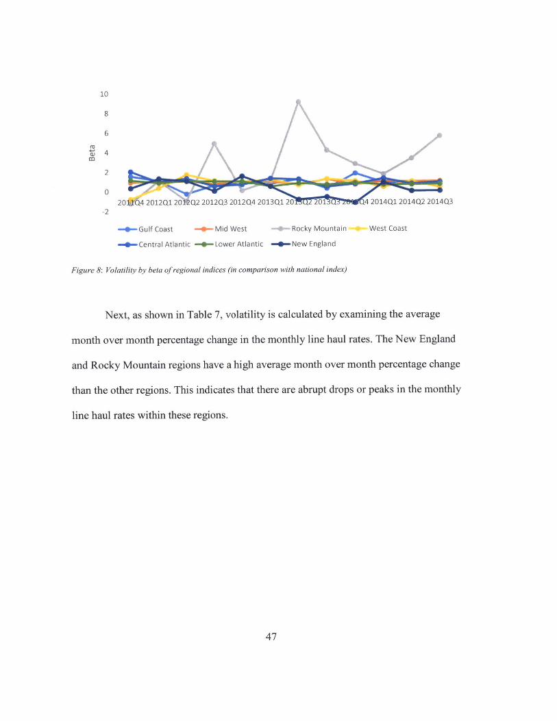
Figure 8 visualizes the volatility of regional indices in comparison with the
national index as a function of time to better identify the trends in the volatility. It
illustrates that the Rocky Mountain region is more volatile than the rest of the markets
that ABC operates in. More specifically, Rocky Mountain peaks in Q3 2012 and Q2
2013. The peaks indicate that the rates are highly volatile in comparison to the national
index, moving in the same direction as the national index. The New England region
exhibits a high degree of volatility in Q2, Q3 and Q4 of 2013 however moving in the
opposite direction of the national index. On the other hand, the Mid West and Lower
Atlantic regions are flat and the beta values consistently hovering around 1 showing that
both these regions behave identical to the national index of ABC and are stable in
comparison to the national index.
46
10
8
6
t4
2
020VIQ4 2012Q1 20 Q2 2012Q3 2012Q4 2013Q1 20 201 4 2014Q1 2014Q2 2014Q3
-2
--- Gulf Coast - Mid West Rocky Mountain West Coast
-*-Central Atlantic p Lower Atlantic -@--New England
Figure 8: Volatility by beta of regional indices (in comparison with national index)
Next, as shown in Table 7, volatility is calculated by examining the average
month over month percentage change in the monthly line haul rates. The New England
and Rocky Mountain regions have a high average month over month percentage change
than the other regions. This indicates that there are abrupt drops or peaks in the monthly
line haul rates within these regions.
47
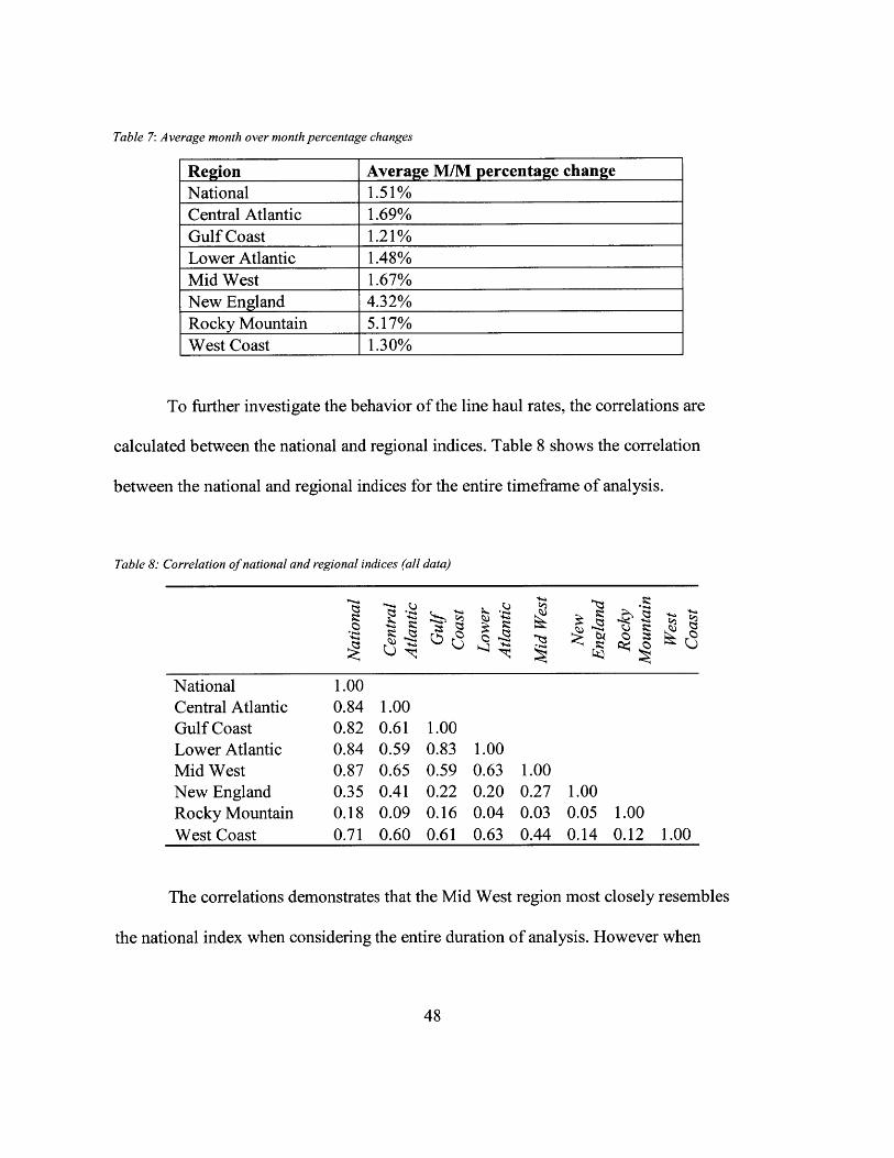
Table 7: Average month over month percentage changes
Region Average M/M percentage changeNational 1.51%Central Atlantic 1.69%Gulf Coast 1.21%Lower Atlantic 1.48%Mid West 1.67%New England 4.32%Rocky Mountain 5.17%West Coast 1.30%
To further investigate the behavior of the line haul rates, the correlations are
calculated between the national and regional indices. Table 8 shows the correlation
between the national and regional indices for the entire timeframe of analysis.
Table 8: Correlation of national and regional indices (all data)
National 1.00Central Atlantic 0.84 1.00Gulf Coast 0.82 0.61 1.00Lower Atlantic 0.84 0.59 0.83 1.00Mid West 0.87 0.65 0.59 0.63 1.00New England 0.35 0.41 0.22 0.20 0.27 1.00Rocky Mountain 0.18 0.09 0.16 0.04 0.03 0.05 1.00West Coast 0.71 0.60 0.61 0.63 0.44 0.14 0.12 1.00
The correlations demonstrates that the Mid West region most closely resembles
the national index when considering the entire duration of analysis. However when
48
examining individual years for instance 2012 as shown in Table 8, the Central Atlantic,
Gulf Coast and Lower Atlantic regions also quite closely resemble the national index.
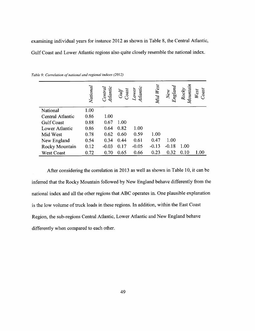
Table 9: Correlation of national and regional indices (2012)
National 1.00Central Atlantic 0.86 1.00Gulf Coast 0.88 0.67 1.00Lower Atlantic 0.86 0.64 0.82 1.00Mid West 0.78 0.62 0.60 0.59 1.00New England 0.54 0.34 0.44 0.61 0.47 1.00Rocky Mountain 0.12 -0.03 0.17 -0.05 -0.13 -0.18 1.00
West Coast 0.72 0.70 0.65 0.66 0.23 0.32 0.10 1.00
After considering the correlation in 2013 as well as shown in Table 10, it can be
inferred that the Rocky Mountain followed by New England behave differently from the
national index and all the other regions that ABC operates in. One plausible explanation
is the low volume of truck loads in these regions. In addition, within the East Coast
Region, the sub-regions Central Atlantic, Lower Atlantic and New England behave
differently when compared to each other.
49
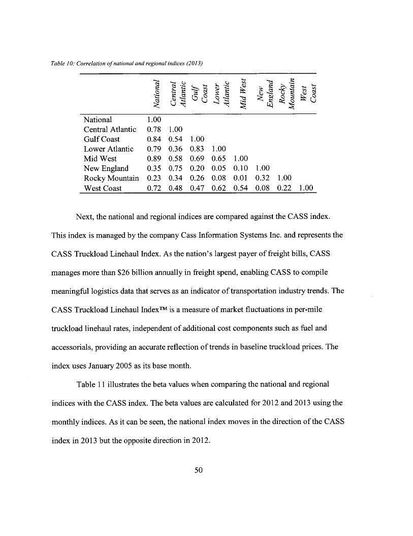
Table 10: Correlation of national and regional indices (2013)
National 1.00Central Atlantic 0.78 1.00Gulf Coast 0.84 0.54 1.00Lower Atlantic 0.79 0.36 0.83 1.00Mid West 0.89 0.58 0.69 0.65 1.00New England 0.35 0.75 0.20 0.05 0.10 1.00Rocky Mountain 0.23 0.34 0.26 0.08 0.01 0.32 1.00West Coast 0.72 0.48 0.47 0.62 0.54 0.08 0.22 1.00
Next, the national and regional indices are compared against the CASS index.
This index is managed by the company Cass Information Systems Inc. and represents the
CASS Truckload Linehaul Index. As the nation's largest payer of freight bills, CASS
manages more than $26 billion annually in freight spend, enabling CASS to compile
meaningful logistics data that serves as an indicator of transportation industry trends. The
CASS Truckload Linehaul IndexTM is a measure of market fluctuations in per-mile
truckload linehaul rates, independent of additional cost components such as fuel and
accessorials, providing an accurate reflection of trends in baseline truckload prices. The
index uses January 2005 as its base month.
Table 11 illustrates the beta values when comparing the national and regional
indices with the CASS index. The beta values are calculated for 2012 and 2013 using the
monthly indices. As it can be seen, the national index moves in the direction of the CASS
index in 2013 but the opposite direction in 2012.
50
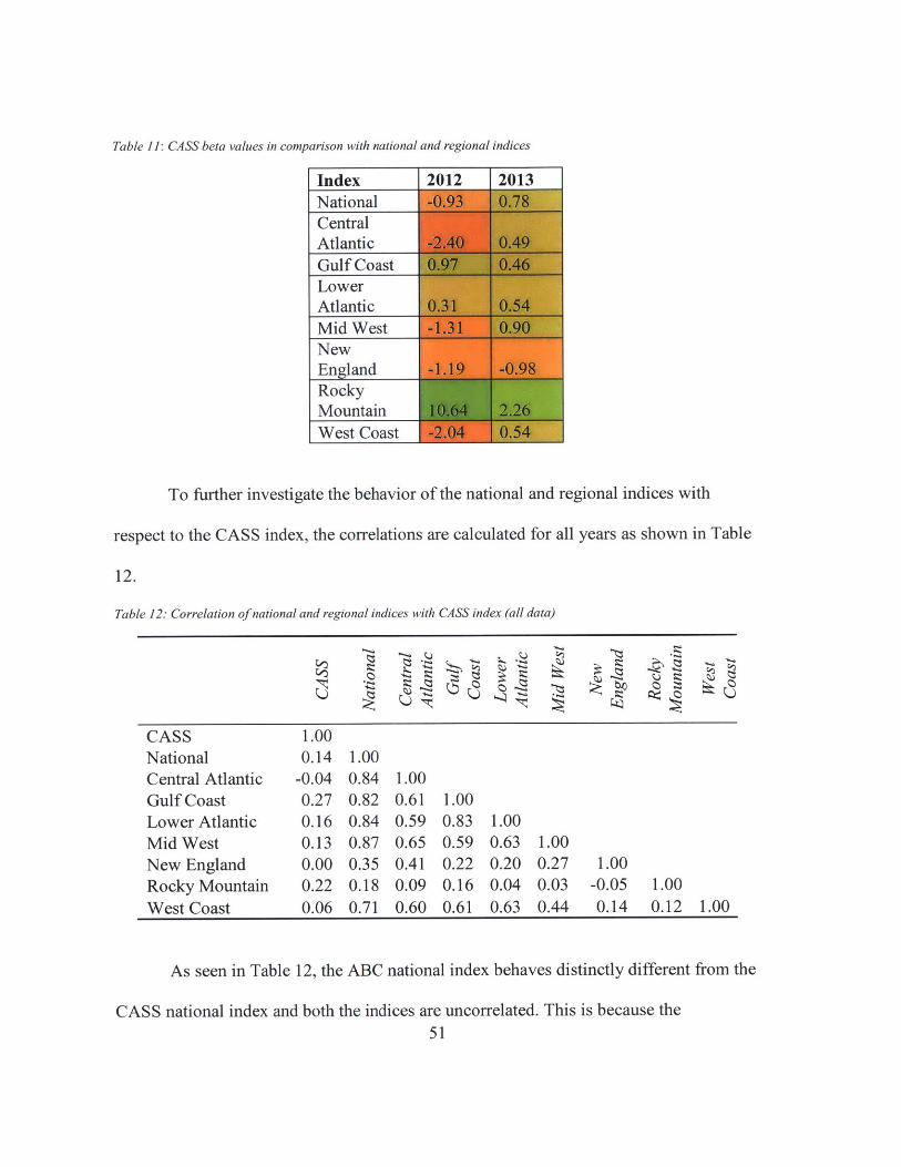
Table 11: CASS beta values in comparison with national and regional indices
Index 2012 2013NationalCentralAtlanticGulf CoastLowerAtlanticMid WestNewEngland
RockyMountainWest Coast
To further investigate the behavior of the national and regional indices with
respect to the CASS index, the correlations are calculated for all years as shown in Table
12.
Table 12: Correlation of national and regional indices with CASS index (all data)
CASS 1.00National 0.14 1.00Central Atlantic -0.04 0.84 1.00Gulf Coast 0.27 0.82 0.61 1.00Lower Atlantic 0.16 0.84 0.59 0.83 1.00Mid West 0.13 0.87 0.65 0.59 0.63 1.00New England 0.00 0.35 0.41 0.22 0.20 0.27 1.00Rocky Mountain 0.22 0.18 0.09 0.16 0.04 0.03 -0.05 1.00West Coast 0.06 0.71 0.60 0.61 0.63 0.44 0.14 0.12 1.00
As seen in Table 12, the ABC national index behaves distinctly different from the
CASS national index and both the indices are uncorrelated. This is because the51
correlation between national and CASS is only 0.14 and for most regions and CASS is
less than 0.25. Therefore the CASS index is not a good representation of ABC's business.
Hence we use ABC's national index for our Beta calculations when examining the
volatility and risk for different regions and lanes.
52
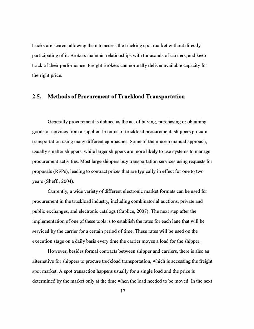
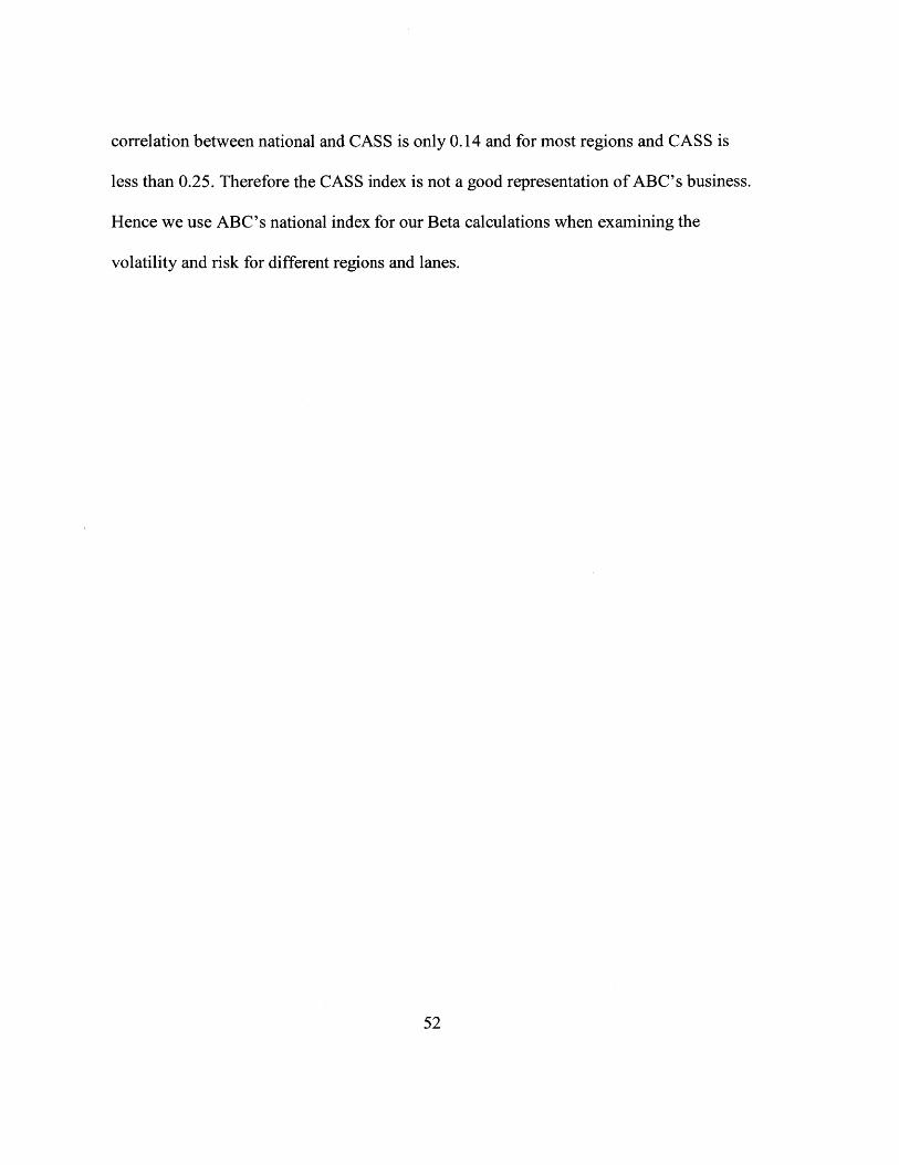
5.4. Lane Characterization
A framework for lane characterization is outlined in Figure 9. According to the
framework, the top 10 risky and less risky lanes are identified by each type of volatility
i.e. coefficient of variation, beta and average month over month percentage change. This
is done for both short haul ( 250 miles) and long haul (>250 miles) lanes. The results are
included in the appendix.
S
S0nr
Top 10 tlanes Bt
hh
aaU.UFigure 9: Lane characterization framework
In general, the Lower Atlantic region consists of more high risk long-haul lanes
than any other region that ABC operates in, based on all three measures of volatility. The
Mid West region consists of more high risk short-term lanes than any other region that
ABC operates in. In addition, the Lower Atlantic region consists of more low risk long-
haul lanes than any other region that ABC operates in, based on all three measures of
53
volatility and the Central Atlantic region consists of more low risk short-haul lanes than
the other regions.
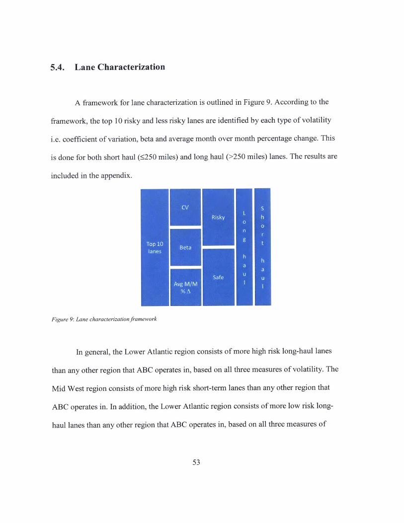
5.5. Factors Related to Volatility
* Beta vs. Distance
Here, beta for each of the lanes in the sample is plotted against the distance of the
lane to investigate the relationship between volatility and distance as shown in
Figure 10.
Region0 S Central Atlantic
4 3 Gulf Coast0 Lower Atlantic
%00 00 Mid West
2 0 -I 0 ct o 0 New England
SRocky Mountain
c0 0 U West Coast
-2
-4
-6
-8
-10
-12
0-14 0
0 200 400 600 800 1000 1200 1400 1600 1800 2000 2200 2400 2600 2800 3000Distance
Figure 10: Beta vs. distance
The R-squared value and the p-value for the overall model for Beta vs. Distance
are 0.04 and 0.02 respectively. This indicates that there the model is insignificant. The p-
values for the various region trend lines (slope coefficient) are in Table 13.
54
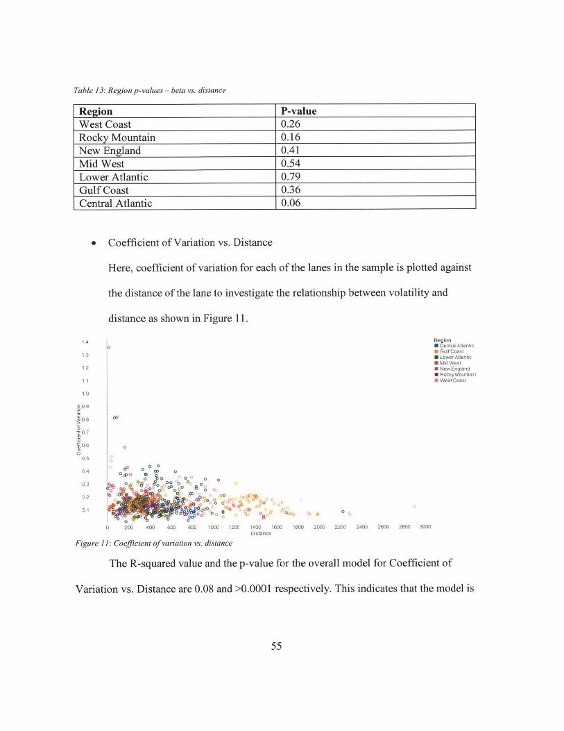
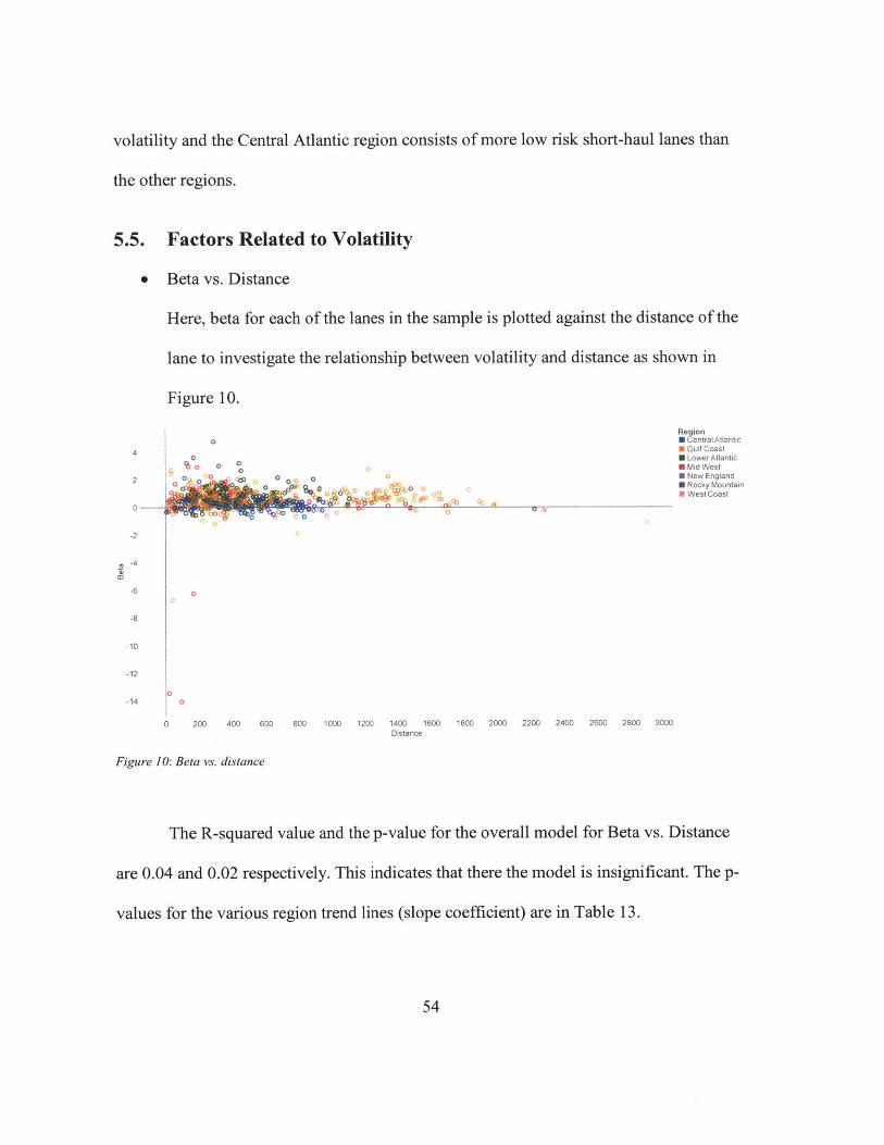
Table 13: Region p-values - beta vs. distance
Region P-valueWest Coast 0.26Rocky Mountain 0.16New England 0.41Mid West 0.54Lower Atlantic 0.79Gulf Coast 0.36Central Atlantic 0.06
* Coefficient of Variation vs. Distance
Here, coefficient of variation for each of the lanes in the sample is plotted against
the distance of the lane to investigate the relationship between volatility and
distance as shown in Figure 11.
1.4 Region1 4IR Central Atlantic
1,3 11 Gulf Coast1 LowerAtlantic* Mid West
11 2 New England* Rocky Mountain
11 West Coast
10
0,9
0.8
06-E0.7
U , 6 I 0
05
04 00D 0
0 %o 0o0 003 0
0 C 0 00
C, 00 4e o
01 o 0 0b0"'0 ~ ~ "s ~ 0
0 200 400 600 800 1000 1200 1400 1600 1800 2000 2200 2400 2600 2800 3000Distance
Figure 11: Coefficient of variation vs. distance
The R-squared value and the p-value for the overall model for Coefficient of
Variation vs. Distance are 0.08 and >0.0001 respectively. This indicates that the model is
55
insignificant. The p-values for the various region trend lines (slope coefficient) are in
Table 14.
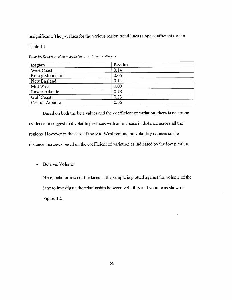
Table 14: Region p-values - coefficient of variation vs. distance
Region P-valueWest Coast 0.14Rocky Mountain 0.06New England 0.14Mid West 0.00Lower Atlantic 0.78Gulf Coast 0.23Central Atlantic 0.66
Based on both the beta values and the coefficient of variation, there is no strong
evidence to suggest that volatility reduces with an increase in distance across all the
regions. However in the case of the Mid West region, the volatility reduces as the
distance increases based on the coefficient of variation as indicated by the low p-value.
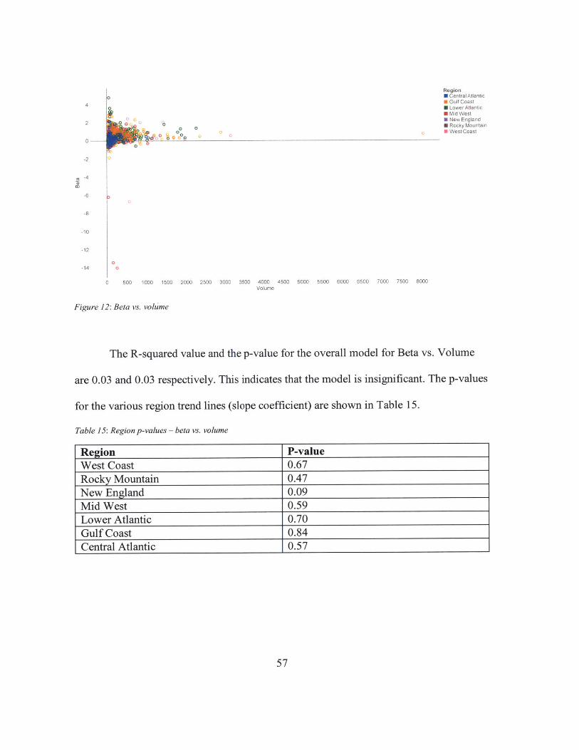
* Beta vs. Volume
Here, beta for each of the lanes in the sample is plotted against the volume of the
lane to investigate the relationship between volatility and volume as shown in
Figure 12.
56
RegionR Central AtlanticE Gulf Coast
4 0 Lower Atlantic0 Mid West0 New England
2 o ERocky Mountain0 West Coast
0 -----2 0
-2
-4
-6
-8
-10
-12
-14 0
0 500 1000 1500 2000 2500 3000 3500 4000 4500 5000 5500 6000 6500 7000 7500 8000Volume
Figure 12: Beta vs. volume
The R-squared value and the p-value for the overall model for Beta vs. Volume
are 0.03 and 0.03 respectively. This indicates that the model is insignificant. The p-values
for the various region trend lines (slope coefficient) are shown in Table 15.
Table 15: Region p-values - beta vs. volume
Region P-valueWest Coast 0.67Rocky Mountain 0.47New England 0.09Mid West 0.59Lower Atlantic 0.70Gulf Coast 0.84Central Atlantic 0.57
57
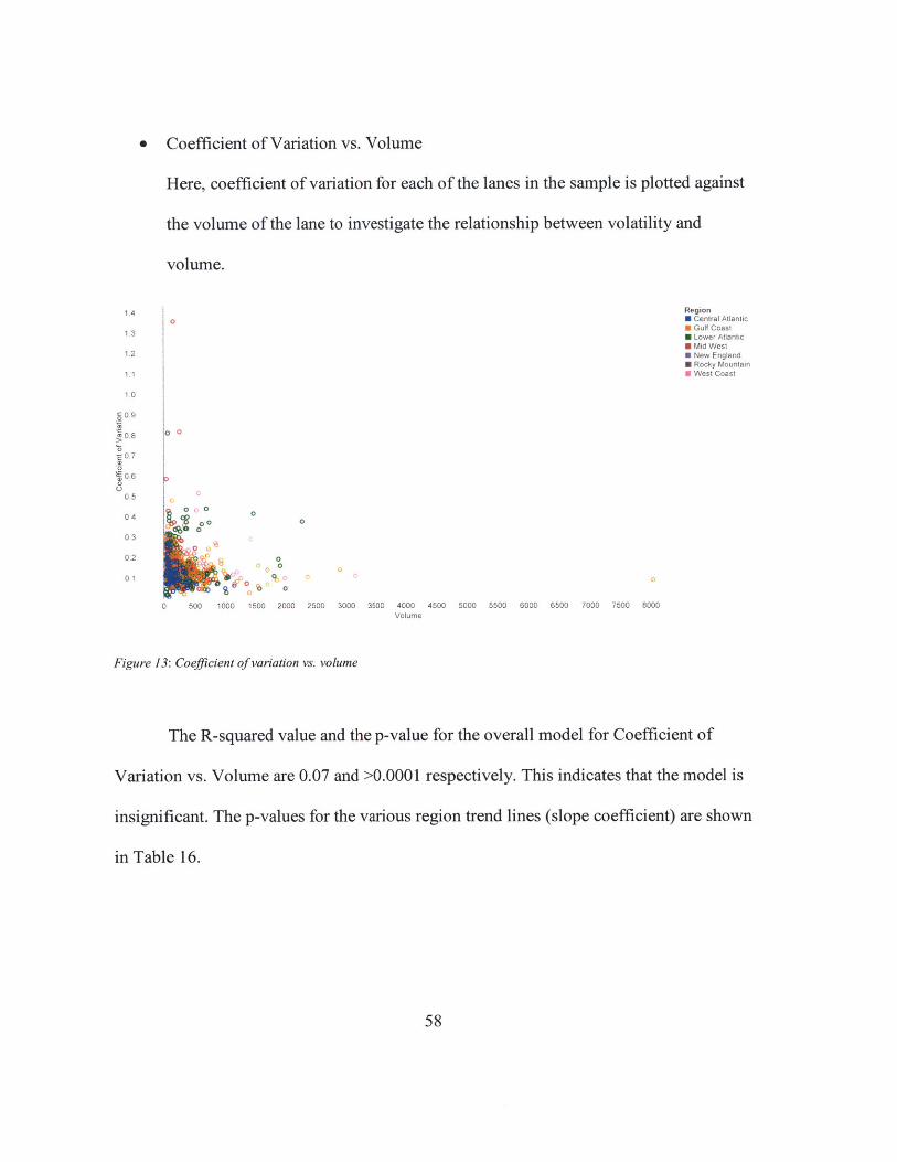
* Coefficient of Variation vs. Volume
Here, coefficient of variation for each of the lanes in the sample is plotted against
the volume of the lane to investigate the relationship between volatility and
volume.
RegionSCentral Atlantic
3 Gulf Coast0 Lower AtlanticN Mid West" New England" Rocky Mountain0 West Coast
10 0
0
0 500 1000 1500 2000 2500 3000 3500 4000 4500 5000 5500 6000 6500 7000 7500 8000Volume
Figure 13: Coefficient of variation vs. volume
The R-squared value and the p-value for the overall model for Coefficient of
Variation vs. Volume are 0.07 and >0.0001 respectively. This indicates that the model is
insignificant. The p-values for the various region trend lines (slope coefficient) are shown
in Table 16.
58
14
1,3
1.2
11
0.90093
0.7
06
0.5
0.4
0,3
02
01
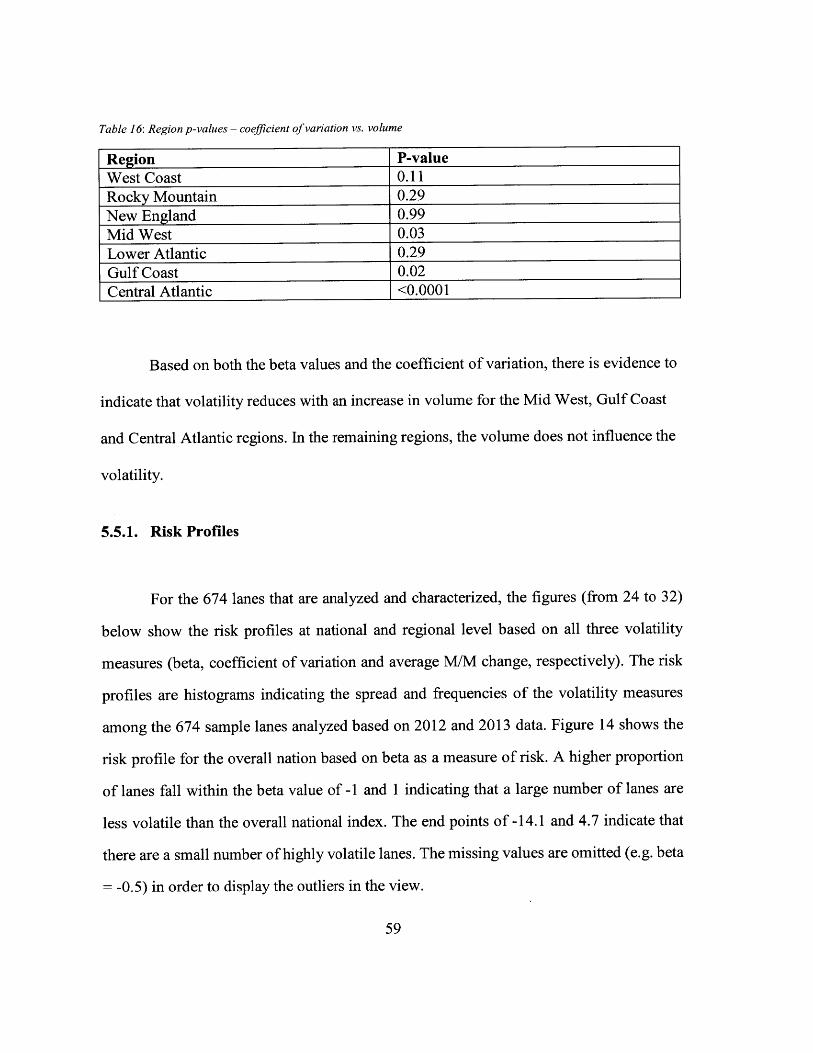
Table 16: Region p-values - coefficient of variation vs. volume
Region P-valueWest Coast 0.11Rocky Mountain 0.29New England 0.99Mid West 0.03Lower Atlantic 0.29Gulf Coast 0.02Central Atlantic <0.0001
Based on both the beta values and the coefficient of variation, there is evidence to
indicate that volatility reduces with an increase in volume for the Mid West, Gulf Coast
and Central Atlantic regions. In the remaining regions, the volume does not influence the
volatility.
5.5.1. Risk Profiles
For the 674 lanes that are analyzed and characterized, the figures (from 24 to 32)
below show the risk profiles at national and regional level based on all three volatility
measures (beta, coefficient of variation and average M/M change, respectively). The risk
profiles are histograms indicating the spread and frequencies of the volatility measures
among the 674 sample lanes analyzed based on 2012 and 2013 data. Figure 14 shows the
risk profile for the overall nation based on beta as a measure of risk. A higher proportion
of lanes fall within the beta value of -1 and 1 indicating that a large number of lanes are
less volatile than the overall national index. The end points of -14.1 and 4.7 indicate that
there are a small number of highly volatile lanes. The missing values are omitted (e.g. beta
= -0.5) in order to display the outliers in the view.
59
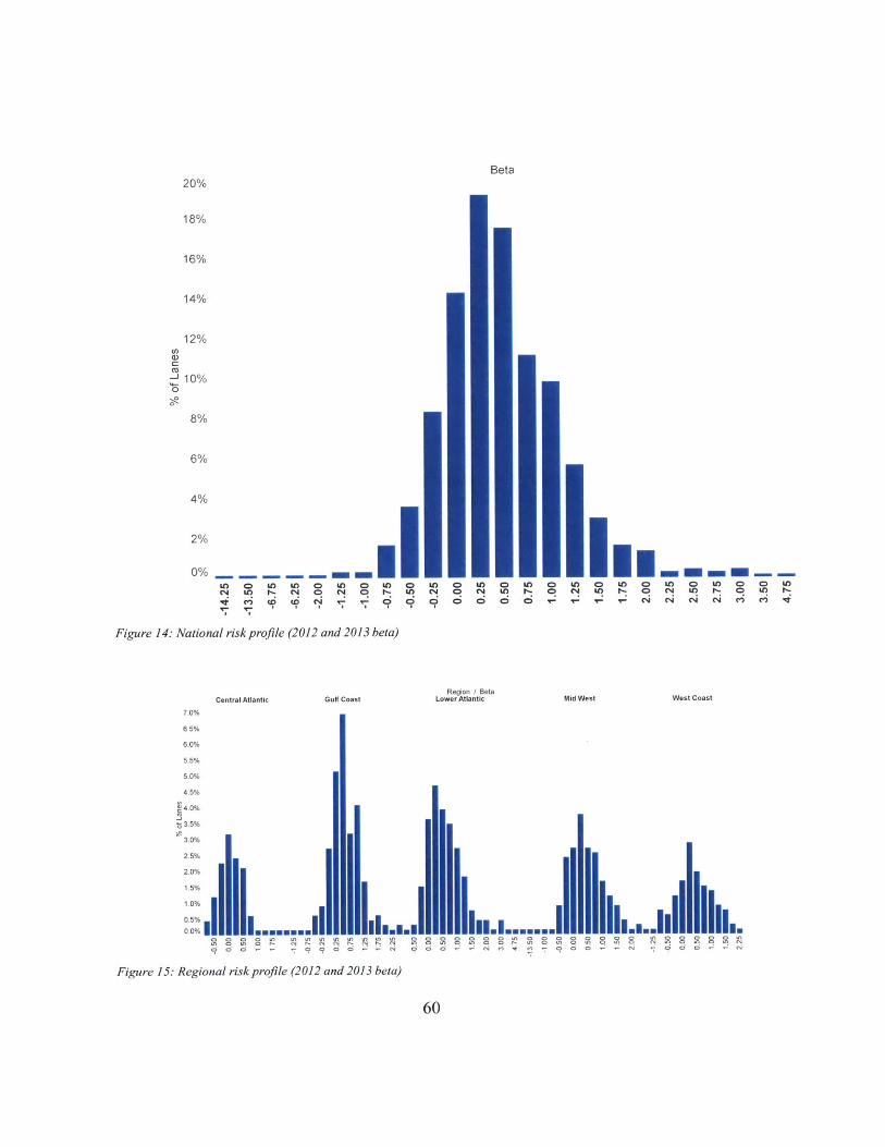
Beta20%
18%
16%
14%
12%
-j 10%0
8%
6%
4%
2%
I
o) a 0 aD0 C 0 D 0 0 C
Central Atlantic Gulf CoastRegion / Beta
Lower Atlantic
I
Mid West
a)I In- 0 0 0 0 0 a)0a 0 0 0 a) 0 0 CD 0 a) 0O -- ~ 00 00 - 00 0- N N N 000t
me9 90%
CD CD
Figure 14: National risk profile (2012 and 2013 beta)
7.0%
65%
6,0%
5.5%
5.0%
4.5%
4.0%
3.5%
3.0%
2.5%
2.0%
1.5%
1 0%
0.5%
0.0%
West Coast
I
Figure 15: Regional risk profile (2012 and 2013 beta)
60
.=======
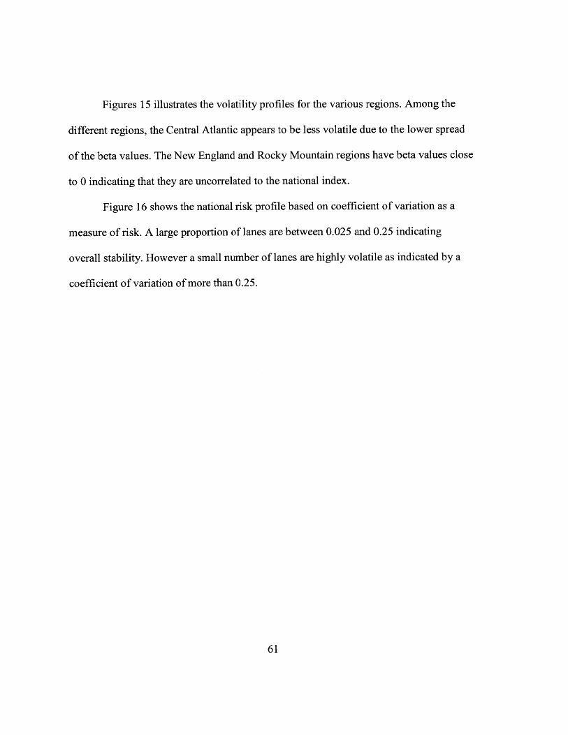
Figures 15 illustrates the volatility profiles for the various regions. Among the
different regions, the Central Atlantic appears to be less volatile due to the lower spread
of the beta values. The New England and Rocky Mountain regions have beta values close
to 0 indicating that they are uncorrelated to the national index.
Figure 16 shows the national risk profile based on coefficient of variation as a
measure of risk. A large proportion of lanes are between 0.025 and 0.25 indicating
overall stability. However a small number of lanes are highly volatile as indicated by a
coefficient of variation of more than 0.25.
61
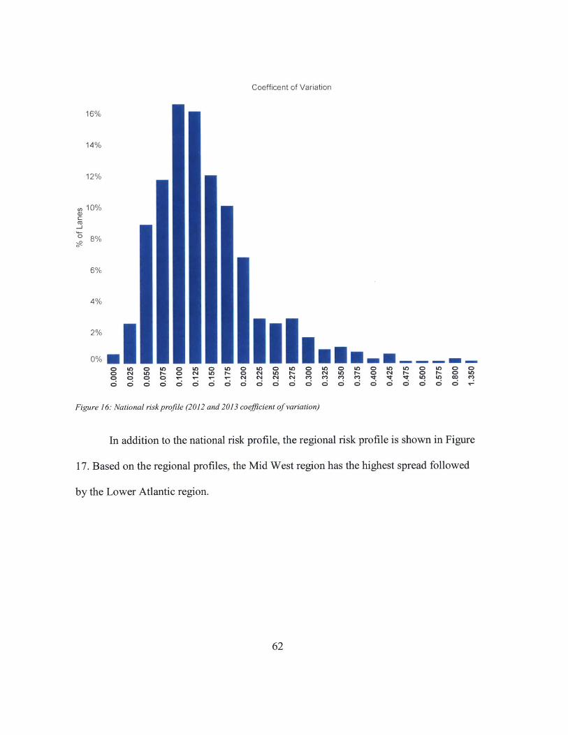
Coefficent of Variation
16%
14%
12%
10%
W)I,-
0
0Q6
U)N
0
010)To
00;
QLO
Figure 16: National risk profile (2012 and 2013 coefficient of variation)
In addition to the national risk profile, the regional risk profile is shown in Figure
17. Based on the regional profiles, the Mid West region has the highest spread followed
by the Lower Atlantic region.
62
liii!!!10 0 U~
10 I~- 0 N 10 I~-N N N C~ (~, C~
666 66666
(I)a3)
0 8%
6%
4%
2%
0 LOO No Q6 C; C
C0
U-1O to
o o
W)
C
1Or-
CLO10

Region / Coefticent of VariationCentral Atlantic Gulf Coast Lower Atlantic Mid West West Coast
5.0%
4 5%
4.0%
3.5%
3.0%
2.5%
2,0%
0 ..... ana.nr -a. ns.. ....-cn
Figure 17: Regional risk profile (2012 and 2013 coefficient of variation)
Figure 18 shows the national risk profile based on the average month/month
percentage changes in the linehaul cost per mile rates. As seen there are some lanes with
extreme values of more than 100%, exhibiting the sporadic movement of spot market
rates in such lanes.
63
Avg M/M % Change
65%
60%
55%
50%
45%
40%C:
D 35%0
30%
25%
20%
15%
10%
5%
0% _
0.000 0.025 0.050 0.075 0.100 0.125 0.150 0.175 0.225 0.275 0.350 0.425 0.525 1.325 1.375Figure 18: National risk profile (2012 and 2013 average M/M % change)
Of the various regions shown in Figures 19, the Mid West region has the highest
spread in this measure.
64
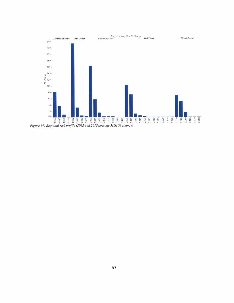
Region / Avg M/M % ChangeCentral Atlantic Gulf Coast Lower Atlantic Mid West West Coast
24%
22%
20%
18%
16%
v 14%
12%
10%
8%
6%
4%
2%
0% I0 - -o U') 0 crc 0 1O 0 cc) 0 U) 0 U) 0 U) U) U) 0 UO 0 U) 0 U) 0 OU') U') n 0 UI) 0 U') U) 00 CN UO P- 0 N U) r- 0 N UO r- 0 N r-_ " 0 N U) 1- 0 N U) 1- r - 0 N UO N N UO
0 D 0 0 - 0 0 0 0 0 0C 0 0 (D 0 0 0 0 0 - -)r 0 0 0 0 c)Figre 6 6Reginalris6 profil 01626 6a6n6 62636 66 a g M-0o % 00age
Figure 19: Regional risk profile (2012 and 2013 average M/M % change)
65
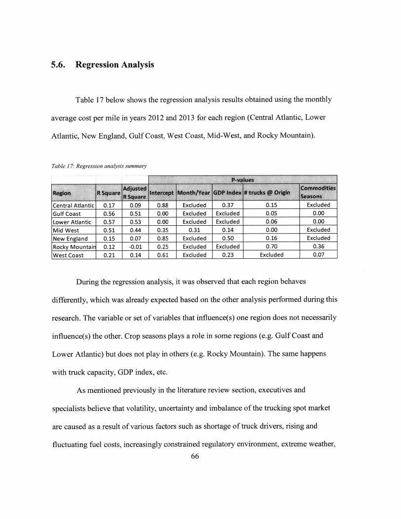
5.6. Regression Analysis
Table 17 below shows the regression analysis results obtained using the monthly
average cost per mile in years 2012 and 2013 for each region (Central Atlantic, Lower
Atlantic, New England, Gulf Coast, West Coast, Mid-West, and Rocky Mountain).
Table 17: Regression analysis summary
Central Atlantic 0.17 0.09 0.88 Excluded 0.37 0.15 ExcludedGulf Coast 0.56 0.51 0.00 Excluded Excluded 0.05 0.00Lower Atlantic 0.57 0.53 0.00 Excluded Excluded 0.06 0.00Mid West 0.51 0.44 0.35 0.31 0.14 0.00 ExcludedNew England 0.15 0.07 0.85 Excluded 0.50 0.16 ExcludedRocky Mountair 0.12 -0.01 0.25 Excluded Excluded 0.70 0.36West Coast 0.21 0.14 0.61 Excluded 0.23 Excluded 0.07
During the regression analysis, it was observed that each region behaves
differently, which was already expected based on the other analysis performed during this
research. The variable or set of variables that influence(s) one region does not necessarily
influence(s) the other. Crop seasons plays a role in some regions (e.g. Gulf Coast and
Lower Atlantic) but does not play in others (e.g. Rocky Mountain). The same happens
with truck capacity, GDP index, etc.
As mentioned previously in the literature review section, executives and
specialists believe that volatility, uncertainty and imbalance of the trucking spot market
are caused as a result of various factors such as shortage of truck drivers, rising and
fluctuating fuel costs, increasingly constrained regulatory environment, extreme weather,
66

increasing operating costs, and many others uncontrollable factors. Most factors are not
easily available to the public, or are not available at all, such as carrier's strategies and
decisions, or even a truck driver's desire to go back home.
Despite the low results in terms of R square, the regression analysis was useful to
give a sense of how different regions are influenced by different reasons. Once
companies understand that, it is possible to put these factors into account when expanding
their business or when agreeing into a long-term contract with a new client, as they could
establish different rates for different times of the year in regions where agricultural
activities play a role for example.
67
6. INSIGHTS AND CONCLUSION
Based on the data analysis in chapter 5, in this section we summarize the key
findings of our research and discuss related recommendations. We propose a series of
methods truckload service providers can use in order to assess and address the risk
involved in their operations.
We will first present the key findings of this research, followed by an example
application of the research in supporting contract pricing and a list of useful
recommendations for assessing and evaluating risk in trucking market operations.
6.1. Key Findings
The different regions as separated based on the Department of Energy Petroleum
Administration for Defense Districts map have unique indices which behave differently
over the timeframe. Based on the three risk measures calculated to determine the
volatility (coefficient of variation, beta and average month/month percentage change), the
Rocky Mountain region is more volatile than the rest of the markets that ABC operates
in. On the other hand, the Mid West and Lower Atlantic regions are stable and have a
similar behavior to the ABC national index.
Correlation analysis during the entire duration of analysis demonstrates that the
Central Atlantic, Gulf Coast, Lower Atlantic and Mid-West regions closely resemble the
national index. Rocky Mountain and New England regions have a low correlation to the
national index. The national and regional indices have a very low correlation to the CASS
index which is an index managed by the company Cass Information Systems Inc. and
represents the Cass Truckload Linehaul Index for the overall market demonstrating that
68
ABC's business is different from rest of the industry and that the CASS index is not an
appropriate representation of its business.
Based on the volatility measured by beta values and the coefficient of variation, it
is found that the Lower Atlantic region consists of the most high risk long haul lanes than
any other region that ABC conducts business in, even though the region as a whole is flat
and stable. In addition, the Mid West region consists of the most high risk short-haul
lanes than any other region that ABC operates in based on both the beta value and the
coefficient of variation even though the region as a whole is flat and stable. The Lower
Atlantic region also consists of the most number of low risk long-haul lanes. The most
number of low risk short-haul lanes are present in the Central Atlantic region which
closely resembles the national index.
The top risky lanes for ABC's business based on 2012 and 2013 measures of
volatility for both short haul and long haul lanes are listed in Table 18.
69
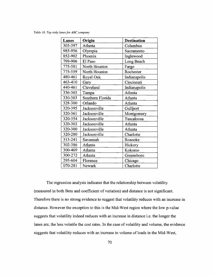
Table 18: Top risky lanes for ABC company
Lanes Origin Destination303-397 Atlanta Columbus985-956 Olympia Sacramento852-902 Phoenix Inglewood799-906 El Paso Long Beach775-581 North Houston Fargo775-559 North Houston Rochester480-461 Royal Oak Indianapolis463-410 Gary Cincinnati440-461 Cleveland Indianapolis336-303 Tampa Atlanta330-303 Southern Florida Atlanta328-300 Orlando Atlanta320-395 Jacksonville Gulfport320-361 Jacksonville Montgomery320-354 Jacksonville Tuscaloosa320-303 Jacksonville Atlanta320-300 Jacksonville Atlanta320-280 Jacksonville Charlotte313-241 Savannah Roanoke302-386 Atlanta Hickory300-469 Atlanta Kokomo300-272 Atlanta Greensboro295-604 Florence Chicago070-281 Newark Charlotte
The regression analysis indicates that the relationship between volatility
(measured in both Beta and coefficient of variation) and distance is not significant.
Therefore there is no strong evidence to suggest that volatility reduces with an increase in
distance. However the exception to this is the Mid-West region where the low p-value
suggests that volatility indeed reduces with an increase in distance i.e. the longer the
lanes are, the less volatile the cost rates. In the case of volatility and volume, the evidence
suggests that volatility reduces with an increase in volume of loads in the Mid-West,
70
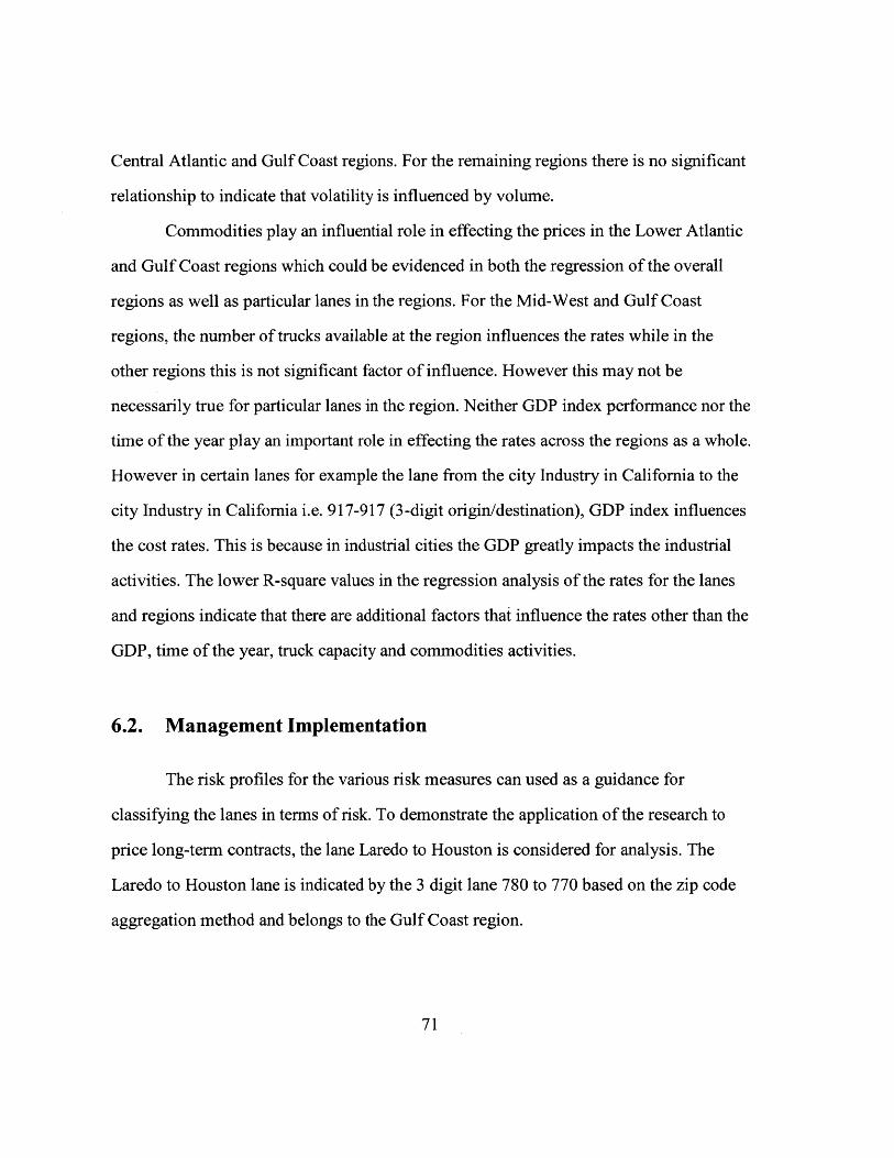
Central Atlantic and Gulf Coast regions. For the remaining regions there is no significant
relationship to indicate that volatility is influenced by volume.
Commodities play an influential role in effecting the prices in the Lower Atlantic
and Gulf Coast regions which could be evidenced in both the regression of the overall
regions as well as particular lanes in the regions. For the Mid-West and Gulf Coast
regions, the number of trucks available at the region influences the rates while in the
other regions this is not significant factor of influence. However this may not be
necessarily true for particular lanes in the region. Neither GDP index performance nor the
time of the year play an important role in effecting the rates across the regions as a whole.
However in certain lanes for example the lane from the city Industry in California to the
city Industry in California i.e. 917-917 (3-digit origin/destination), GDP index influences
the cost rates. This is because in industrial cities the GDP greatly impacts the industrial
activities. The lower R-square values in the regression analysis of the rates for the lanes
and regions indicate that there are additional factors that influence the rates other than the
GDP, time of the year, truck capacity and commodities activities.
6.2. Management Implementation
The risk profiles for the various risk measures can used as a guidance for
classifying the lanes in terms of risk. To demonstrate the application of the research to
price long-term contracts, the lane Laredo to Houston is considered for analysis. The
Laredo to Houston lane is indicated by the 3 digit lane 780 to 770 based on the zip code
aggregation method and belongs to the Gulf Coast region.
71
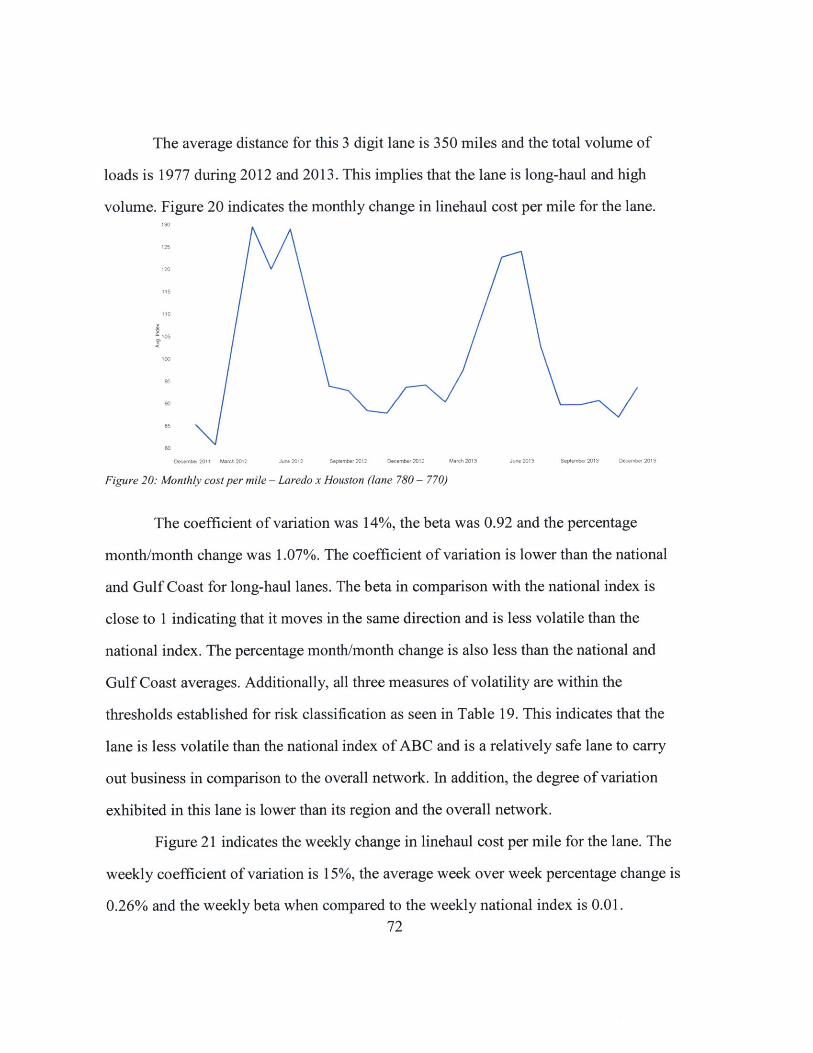
The average distance for this 3 digit lane is 350 miles and the total volume of
loads is 1977 during 2012 and 2013. This implies that the lane is long-haul and high
volume. Figure 20 indicates the monthly change in linehaul cost per mile for the lane.
125
120
115
110
1 05
91t
90
85
80
December 2011 March 2012 June 2012 September 2012 December 2012 March 2013 June 2013 September 2013 December 2013
Figure 20: Monthly cost per mile - Laredo x Houston (lane 780 - 770)
The coefficient of variation was 14%, the beta was 0.92 and the percentage
month/month change was 1.07%. The coefficient of variation is lower than the national
and Gulf Coast for long-haul lanes. The beta in comparison with the national index is
close to 1 indicating that it moves in the same direction and is less volatile than the
national index. The percentage month/month change is also less than the national and
Gulf Coast averages. Additionally, all three measures of volatility are within the
thresholds established for risk classification as seen in Table 19. This indicates that the
lane is less volatile than the national index of ABC and is a relatively safe lane to carry
out business in comparison to the overall network. In addition, the degree of variation
exhibited in this lane is lower than its region and the overall network.
Figure 21 indicates the weekly change in linehaul cost per mile for the lane. The
weekly coefficient of variation is 15%, the average week over week percentage change is
0.26% and the weekly beta when compared to the weekly national index is 0.01.72
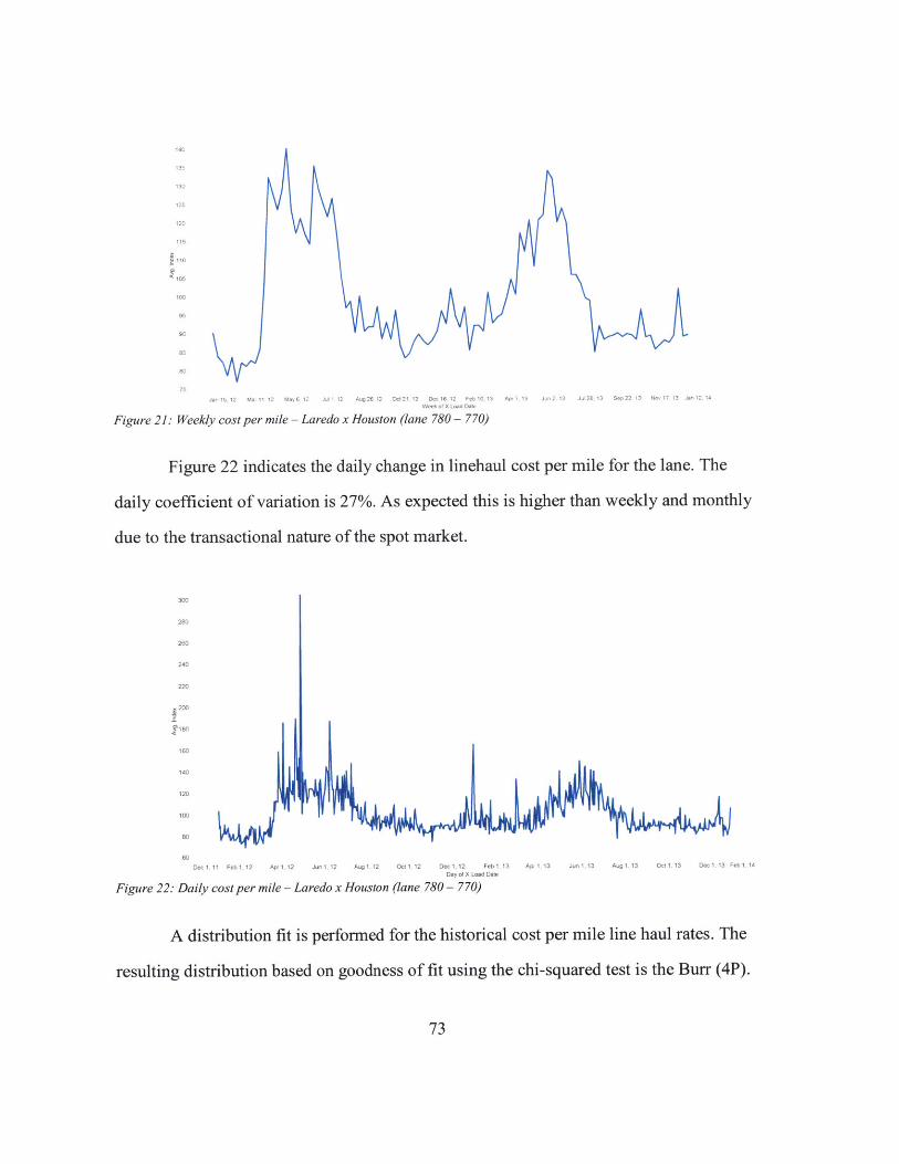
140
135
130
125
120
115
110
105
100
95
0
65
Jan 15 12 Ma 11 12 May 6 12 Jul 1 12 Aug 26 12 Oct 21, 12 Dec 16 2 Fb 10 13 Apr 7.1 J1.13 6441 13 Nov 113 Jan 12, 14
Figure 21: Weekly cost per mile - Laredo x Houston (lane 780 - 770)
Figure 22 indicates the daily change in linehaul cost per mile for the lane. The
daily coefficient of variation is 27%. As expected this is higher than weekly and monthly
due to the transactional nature of the spot market.
300
280
260
240
220
200
160
140
120
100
80
60Dec 1, 11 Feb 1, 12 Apr 1, 12 Jun 1. 12 Aug 1. 12 Oct 1, 12 Dec 1, 12 Feb 1, 13 Ap, 1, 13 Jun 1, 13 Aug 1. 13 Oct 1, 13 Dec 1, 13 Feb 1. 14
Day of X Load Date
Figure 22: Daily cost per mile - Laredo x Houston (lane 780 - 770)
A distribution fit is performed for the historical cost per mile line haul rates. The
resulting distribution based on goodness of fit using the chi-squared test is the Burr (4P).
73
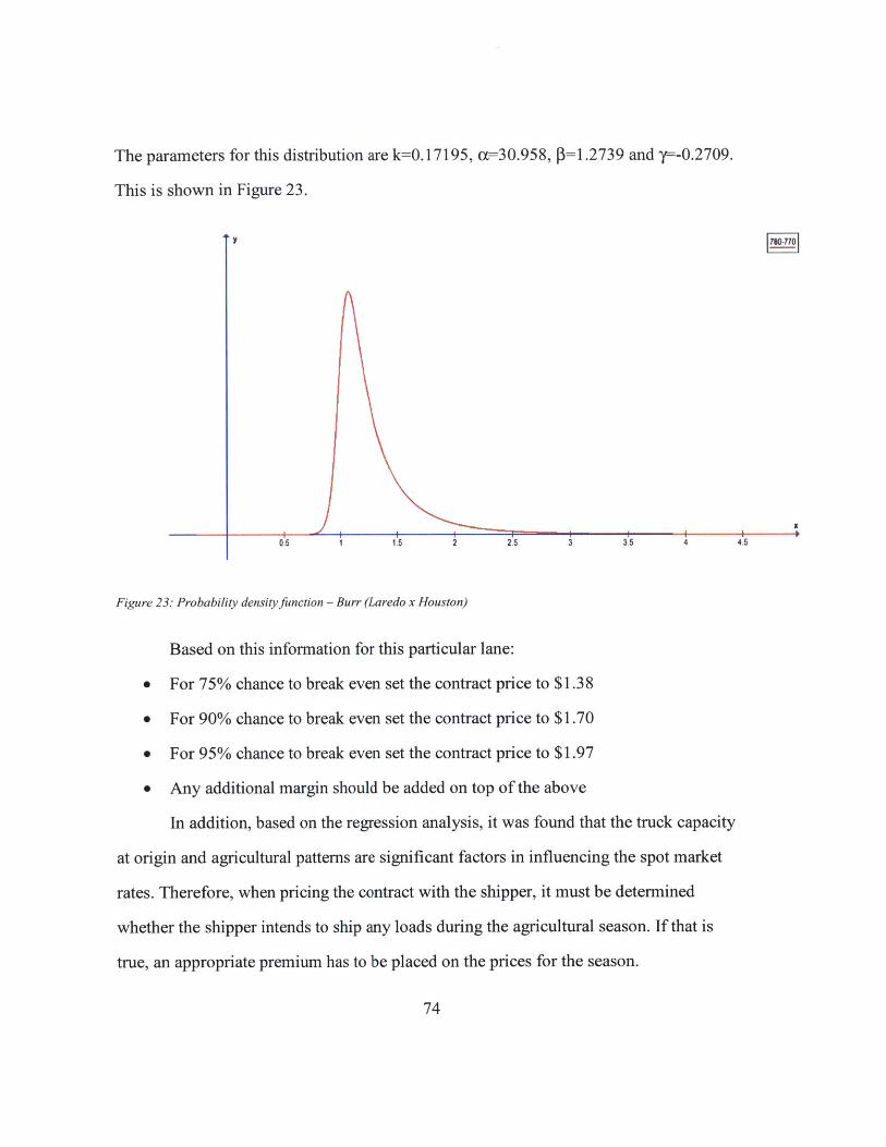
The parameters for this distribution are k=O.17195, w=30.958, =1.2739 and y=-0. 2 7 09 .
This is shown in Figure 23.
YI
05 .5 2 2.5 3 3,5 4 4.5
Figure 23: Probability density function - Burr (Laredo x Houston)
Based on this information for this particular lane:
* For 75% chance to break even set the contract price to $1.38
* For 90% chance to break even set the contract price to $1.70
* For 95% chance to break even set the contract price to $1.97
* Any additional margin should be added on top of the above
In addition, based on the regression analysis, it was found that the truck capacity
at origin and agricultural patterns are significant factors in influencing the spot market
rates. Therefore, when pricing the contract with the shipper, it must be determined
whether the shipper intends to ship any loads during the agricultural season. If that is
true, an appropriate premium has to be placed on the prices for the season.
74
6.3. Recommendations and Conclusion
Below are key recommendations for 3PL businesses:
Volatility characterization is holistic: As seen in the analysis, it is essential to take
a holistic approach when assessing volatility and risk. In this case three measures i.e.
coefficient of variation, beta and average month/month percentage change were
developed to quantify the volatility in lanes and regions and characterize them. This
ensured that though a lane may appear to be "safe" under one type of volatility measure,
its "risk" as measured by another type of volatility measure is accurately captured.
Volatility characterization is geographic: As seen in the analysis, volatility varies
geographically across the various regions. Some regions such as the Rocky Mountain and
New England are evidently more volatile than rest of the markets. Hence, it is important
to view the regional differences in volatility when assessing the risk faced by the 3PL
business. In situations where individual lanes do not follow the regional characteristics,
sub-region categorization and individual lane based volatility analysis will help improve
the precision.
Volatility factors vary geographically: The factors that influence the volatility in
one region or lane do not necessarily impact the other regions or lanes. Hence, the factors
have to be tested for their influence across the various regions and lanes to understand
volatility patterns.
75
Our key contributions from this research are:
" Demonstrated some of the potential uses of historical transactions data by
non-asset backed 3PL companies to assess and mitigate risk
" Utilization of coefficient of variation, beta value and average
month/month percentage change to measure volatility in linehaul rates
" Characterization of regions and lanes based on volatility
" Development of risk profiles for regions and individual lanes
" Utilization of historical linehaul rates distributions to price contracts
* Identification of factors such as agricultural activity and truck availability
that influence the volatility in certain regions
6.4. Future Research
This research reveals many interesting opportunities for future work. For
example:
" Incorporation of other external factors that might influence spot market
rates volatility
" Identify other potential segmentation in terms of distance, regions, lanes,
corridors, time periods (monthly vs. weekly), and others
" Investigation of connections between financial markets and linehaul spot
price markets
76

* Combining data from more brokers and 3PL providers, and therefore
adding more data to the analysis, would provide a more complete outlook
of the market
77
REFERENCES
ATA Truck Tonnage Index Gained 1.1% in March (n.d). Retrieved May 8, 2015, fromhttp://www.trucking.org/article.aspx?uid=3ff~e309-8531-4271 -bfcf-e39d9955a677.
Bahhouth, V., Maysami, R., & Khoueiri, R. (2010). Significance of Beta and FinancialMeasures in Predicting the Riskiness of S&p 500 Stocks During the Downturn of Year2008. International Journal of Business, Accounting, & Finance, 4(2), 12-18.
Bignell, A. (2013). Characteristics of spot-market rate indexes for truckload transportation/ by Andrew Bignell. c2013.
Branger, N., & Schlag, C. (2007). Option Betas:: Risk Measures for Options. InternationalJournal of Theoretical & Applied Finance, 10(7), 1137-1157.
Caplice, C. (2007). Electronic Markets for Truckload Transportation. Production &Operations Management, 16(4), 423-436.
Cassidy, W. B. (2010). Truck Pricing Seeks Higher Gear. Journal Of Commerce(15307557), 11(25), 10-13.
Cassidy, W. B. (2014). Trucking Hits a Reset Button. Journal of Commerce (15307557),15(9), 12-17.
Garrido, R. A. (2007). Procurement of transportation services in spot markets under adouble-auction scheme with elastic demand. Transportation Research Part B 41 (2007)1067-1078.
Gillen, D., & Mantin, B. (2009). Price volatility in the airline markets. TransportationResearch Part E, 45693-709. doi:10.1016/j.tre.2009.04.014
Harding, M. J. (2005). Can shippers and carriers benefit from more robust transportationplanning methodologies? / by Matthew James Harding. c2005.
Jing Dai, Sriboonchitta, S., & Ting Li. (2012). Modeling the Volatility in China's RailwayFreight Volume Based on Conditional Volatility Model. International Journal of IntelligentTechnologies & Applied Statistics, 5(2), 157-166.
Kafarski, L., & Caruso, D. A., Jr. (2012). Effects of truckload freight assignment methodson carrier capacity and pricing / by Lukasz Kafarski and David Allen Caruso, Jr. c2012.
78
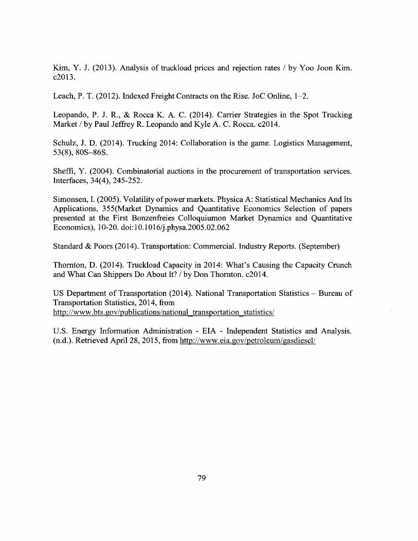
Kim, Y. J. (2013). Analysis of truckload prices and rejection rates / by Yoo Joon Kim.c2013.
Leach, P. T. (2012). Indexed Freight Contracts on the Rise. JoC Online, 1-2.
Leopando, P. J. R., & Rocca K. A. C. (2014). Carrier Strategies in the Spot TruckingMarket / by Paul Jeffrey R. Leopando and Kyle A. C. Rocca. c2014.
Schulz, J. D. (2014). Trucking 2014: Collaboration is the game. Logistics Management,53(8), 80S-86S.
Sheffi, Y. (2004). Combinatorial auctions in the procurement of transportation services.Interfaces, 34(4), 245-252.
Simonsen, I. (2005). Volatility of power markets. Physica A: Statistical Mechanics And ItsApplications, 355(Market Dynamics and Quantitative Economics Selection of paperspresented at the First Bonzenfreies Colloquiumon Market Dynamics and QuantitativeEconomics), 10-20. doi:10.1016/j.physa.2005.02.062
Standard & Poors (2014). Transportation: Commercial. Industry Reports. (September)
Thornton, D. (2014). Truckload Capacity in 2014: What's Causing the Capacity Crunchand What Can Shippers Do About It? / by Don Thornton. c2014.
US Department of Transportation (2014). National Transportation Statistics - Bureau ofTransportation Statistics, 2014, fromhttp://www.bts.gov/publications/national transportation statistics/
U.S. Energy Information Administration - EIA - Independent Statistics and Analysis.(n.d.). Retrieved April 28, 2015, from http://www.eia.gov/petroleum/gasdiesel/
79
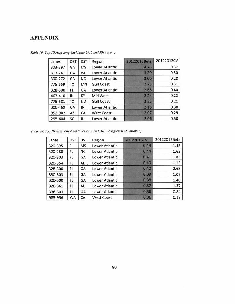
APPENDIX
Table 19: Top 10 risky long-haul lanes 2012 and 2013 (beta)
Lanes OST DST Region303-397 GA MS Lower Atlantic313-241 GA VA Lower Atlantic300-272 GA NC Lower Atlantic775-559 TX MN Gulf Coast328-300 FL GA Lower Atlantic463-410 IN KY Mid West775-581 TX ND Gulf Coast300-469 GA IN Lower Atlantic852-902 AZ CA West Coast295-604 SC IL Lower Atlantic
Table 20: Top 10 risky long-haul lanes 2012 and 2013 (coefficient of variation)
Lanes OST DST Region320-395 FL MS Lower Atlantic320-280 FL NC Lower Atlantic320-303 FL GA Lower Atlantic320-354 FL AL . Lower Atlantic
328-300 FL GA Lower Atlantic330-303 FL GA Lower Atlantic320-300 FL GA Lower Atlantic320-361 FL AL Lower Atlantic336-303 FL GA Lower Atlantic985-956 WA CA West Coast
20122013CV
0.32
0.300.28
0.31
0.40
0.22
0.21
0.300.290.30
20122013Beta
1.45
1.631.831.132.681.07
1.40
1.37
0.84
0.19
80
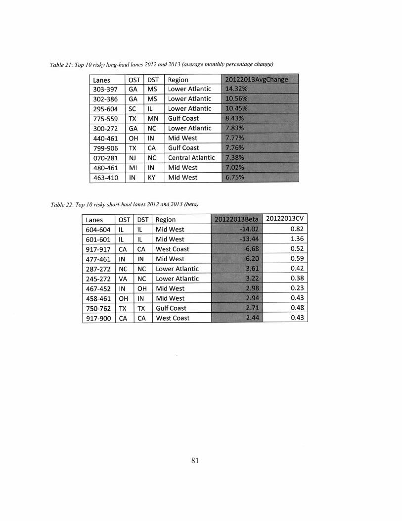
Table 21: Top 10 risky long-haul lanes 2012 and 2013 (average monthly percentage change)
Lanes OST DST Region303-397 GA MS Lower Atlantic302-386 GA MS Lower Atlantic295-604 SC IL Lower Atlantic775-559 TX MN Gulf Coast300-272 GA NC Lower Atlantic440-461 OH IN Mid West799-906 TX CA Gulf Coast070-281 NJ NC Central Atlantic480-461 MI IN Mid West463-410 IN KY Mid West
Table 22: Top 10 risky short-haul lanes 2012 and 2013 (beta)
Lanes OST DST Region604-604 IL IL Mid West601-601 IL IL Mid West917-917 CA CA West Coast477-461 IN IN Mid West287-272 NC NC Lower Atlantic245-272 VA NC Lower Atlantic467-452 IN OH Mid West458-461 OH IN Mid West750-762 TX TX Gulf Coast917-900 CA CA West Coast
20122013CV
0.82
1.36
0.52
0.59
0.42
0.380.230.43
0.48
0.43
81
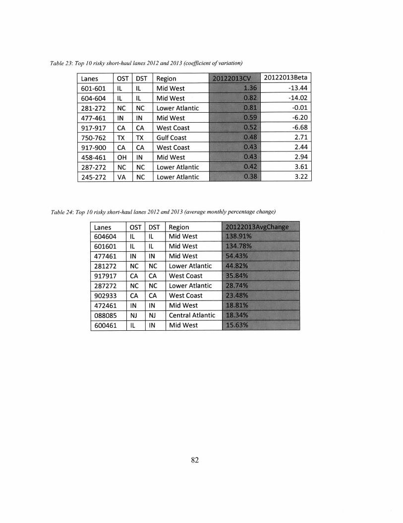
Table 23: Top 10 risky short-haul lanes 2012 and 2013 (coefficient of variation)
Lanes OST DST Region601-601 IL IL Mid West604-604 IL IL Mid West281-272 NC NC Lower Atlantic477-461 IN IN Mid West917-917 CA CA West Coast750-762 TX TX Gulf Coast917-900 CA CA West Coast458-461 OH IN Mid West287-272 NC NC Lower Atlantic245-272 VA NC Lower Atlantic
Table 24: Top 10 risky short-haul lanes
20122013Beta
-13.44
-14.02
-0.01-6.20
-6.682.71
2.44
2.94
3.61
3.22
2012 and 2013 (average monthly percentage change)
Lanes OST DST Region
604604 IL IL Mid West
601601 IL IL Mid West
477461 IN IN Mid West
281272 NC NC Lower Atlantic
917917 CA CA West Coast
287272 NC NC Lower Atlantic
902933 CA CA West Coast472461 IN IN Mid West
088085 NJ NJ Central Atlantic
600461 IL IN Mid West
82
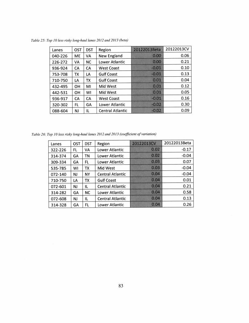
Table 25: Top 10 less risky long-haul lanes 2012 and 2013 (beta)
Lanes OST DST Region040-226 ME VA New England226-272 VA NC Lower Atlantic936-924 CA CA West Coast
753-708 TX LA Gulf Coast710-750 LA TX Gulf Coast432-495 OH MI Mid West442-531 OH WI Mid West
936-917 CA CA West Coast
320-302 FL GA Lower Atlantic
088-604 NJ IL Central Atlantic
Table 26: Top 10 less risky long-haul lanes
20122013CV
0.06
0.21
0.10
0.13
0.04
0.12
0.05
0.16
0.30
0.09
2012 and 2013 (coefficient of variation)
Lanes OST DST Region
322-226 FL VA Lower Atlantic
314-374 GA TN Lower Atlantic
309-334 GA FL Lower Atlantic
535-785 WI TX Mid West
072-140 NJ NY Central Atlantic
710-750 LA TX Gulf Coast
072-601 NJ IL Central Atlantic
314-282 GA NC Lower Atlantic
072-608 NJ IL Central Atlantic
314-328 GA FL Lower Atlantic
20122013Beta
-0.17
-0.04
0.07
-0.04
-0.04
0.01
0.21
0.580.13
0.26
83

Table 27: Top 10 less risky long-haul lanes 2012 and 2013 (average monthly percentage change)
Lanes OST DST Region780799 TX TX Gulf Coast
775641 TX MO Gulf Coast
322226 FL VA Lower Atlantic
314374 GA TN Lower Atlantic
767785 TX TX Gulf Coast
072601 NJ IL Central Atlantic
314370 GA TN Lower Atlantic
767799 TX TX Gulf Coast
805741 CO OK Rocky Mountain
072140 NJ NY Central Atlantic
Table 28: Top 10 less risky short-haul lanes 2012 and 2013 (beta)
Lanes OST DST Region
178-226 PA VA Central Atlantic
229-226 VA VA Lower Atlantic
281-272 NC NC Lower Atlantic
752-767 TX TX Gulf Coast
436-482 OH MI Mid West
325-325 FL FL Lower Atlantic
177-151 PA PA Central Atlantic
175-226 PA VA Central Atlantic
956-945 CA CA West Coast
182-226 PA VA Central Atlantic
20122013CV
0.01
0.030.81
0.06
0.08
0.07
0.14
0.11
0.22
0.07
84
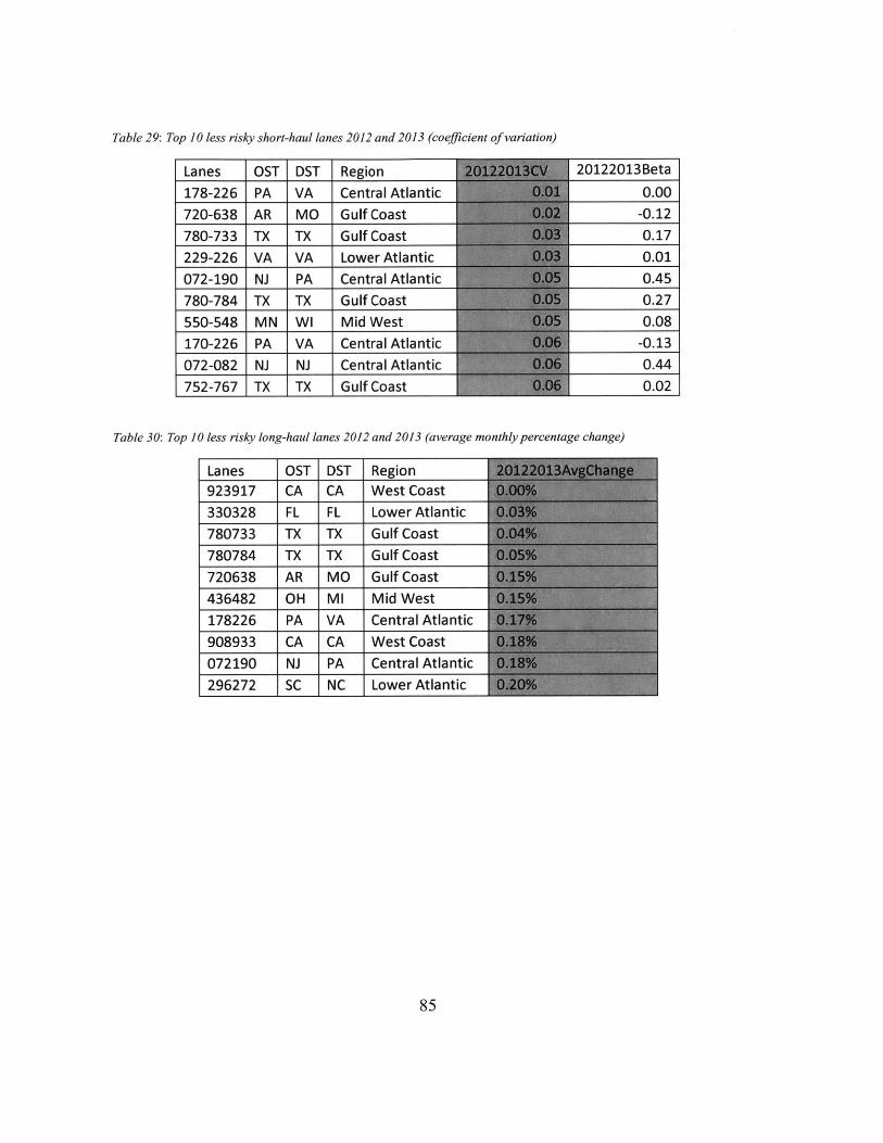
Table 29: Top 10 less risky short-haul lanes 2012 and 2013 (coefficient of variation)
Lanes OST DST Region
178-226 PA VA Central Atlantic
720-638 AR MO Gulf Coast
780-733 TX TX Gulf Coast
229-226 VA VA Lower Atlantic
072-190 NJ PA Central Atlantic
780-784 TX TX Gulf Coast
550-548 MN WI Mid West
170-226 PA VA Central Atlantic
072-082 NJ NJ Central Atlantic
752-767 TX TX Gulf Coast
20122013Beta
0.00-0.12
0.17
0.010.45
0.27
0.08-0.13
0.44
0.02
Table 30: Top 10 less risky long-haul lanes 2012 and 2013 (average monthly percentage change)
Lanes OST DST Region923917 CA CA West Coast
330328 FL FL Lower Atlantic
780733 TX TX Gulf Coast
780784 TX TX Gulf Coast
720638 AR MO Gulf Coast
436482 OH MI Mid West
178226 PA VA Central Atlantic
908933 CA CA West Coast
072190 NJ PA Central Atlantic
296272 SC NC Lower Atlantic
85