Data-centric Transformations for LocalityEnhancement

Induprakas KodukulaKeshav Pingali

September 26, 2002

AbstractOn modern computers, the performance of programs is often limited by

memory latency rather than by processor cycle time. To reduce the impactof memory latency, the restructuring compiler community has developedlocality-enhancing program transformations such as loop permutation andtiling. These transformations work well for perfectly nested loops (loops inwhich all assignment statements are contained in the innermost loop), buttheir performance on codes such as matrix factorizations that contain imper-fectly nested loops leaves much to be desired. In this paper, we propose analternative approach called data-centric transformation. Instead of reason-ing directly about the control structure of the program, a compiler using thedata-centric approach chooses an order for the arrival of data elements in thecache, determines what computations should be performed when that dataarrives, and generates the appropriate code. At runtime, program executionwill automatically pull data into the cache in an order that corresponds ap-proximately to the order chosen by the compiler; since statements that toucha data structure element are scheduled close together, locality is improved.

The idea of data-centric transformation is very general, and in this pa-per, we discuss a particular transformation called data-shackling. We haveimplemented shackling in the SGI MIPSPro compiler which already has asophisticated implementation of control-centric transformations for localityenhancement. We present experimental results on the SGI Octane compar-ing the performance of the two approaches, and show that for dense numeri-cal linear algebra codes, data-shackling does better by factors of two to five.

Keywords: Locality enhancement, restructuring compilers, caches, pro-gram transformation

1

1

1 Introduction

The memory system of modern computers is hierarchical in organization. Sincethe latency of data accesses may increase by an order of magnitude or more fromone level of the hierarchy to the next, programs run well on such machines onlyif most of their accesses are satisfied by the faster levels of the memory hierarchy.For this to happen, a program must exhibit locality of reference. If accesses toa memory location are clustered together in time, the program is said to exhibittemporal locality, which is beneficial since it is likely that all these accesses otherthan the first one will be satisfied by the faster levels of the memory hierarchy. Ifthe addresses of memory locations accessed successively by a program are closeto each other, the program is said to exhibit spatial locality, which is beneficialbecause the unit of transfer between different levels of the memory hierarchy is aline or block, so successive memory accesses to addresses that are close to eachother are likely to be satisfied mostly by the faster levels of the memory hierarchy.

For many applications, straight-forward coding of standard algorithms resultsin programs that exhibit poor locality of reference. Unfortunately, taking localityinto consideration when writing programs complicates the task of programmingenormously. One solution is to write optimized, machine-specific routines only forcertain core operations, and code all other applications in a high-level language,invoking these routines when appropriate. This achieves high performance with-out sacrificing portability of the application code. The numerical analysis commu-nity has followed this approach by hand coding machine-specific programs for theBasic Linear Algebra Subroutines (BLAS),(15) and layering all other dense numer-ical linear algebra software on top of these routines. However, most applicationshave to be recoded at a fundamental level to use such libraries. To exploit theBLAS for example, the numerical analysis community has had to invest consider-able effort in designing block algorithms and implementing them in the LAPACKlibrary,(2) as described in Section 3. Furthermore, these libraries are not usefulin writing other applications such as PDE solvers that use explicit methods sincethese codes cannot be restructured to expose BLAS operations.

1This work was supported by NSF grants EIA-9726388, ACI-9870687, EIA-9972853, andACI-0085969.Corresponding author: Keshav Pingali, Department of Computer Science, Cornell University,Ithaca, NY 14853; email:pingali@cs.cornell.edu, tel: (607)-255-7203, fax: (607)-255-4428.

2

The compiler community has explored a more general-purpose approach inwhich locality is enhanced by automatic program transformation. To explain thistechnology, it is necessary to introduce the following definitions.

Definition 1.0.1 A perfectly nested loop nest is a loop nest in which all assign-ment statements are contained in the innermost loop of the loop nest. The matrixmultiplication code shown in Figure 1(e) is an example.

An imperfectly nested loop nest is a loop nest in which one or more assignmentstatements in contained in some but not all of the loops of the loop nest. Thetriangular solve code in Figure 1(d) is an example.

An instance of a statement is an execution of that statement for particularindex values of its surrounding loops.

For perfectly nested loops, there is an elegant matrix-based theory for synthe-sizing linear loop transformations for locality enhancement.(4, 6, 8, 10, 14, 16, 20, 26, 28, 32)

These transformations, followed by loop tiling,(34) are performed routinely bymany production compilers such as the SGI MIPSPro. The theory of loop trans-formations is much less developed for imperfectly nested loops. Some compilersuse transformations like jamming, distribution and statement sinking(33, 34) to con-vert imperfectly nested loops into perfectly nested loops, and enhance localityby suitably transforming the resulting perfectly nested loops. However, there isno systematic theory for determining the order in which these imperfectly nestedloop transformations must be applied, and the quality of the final tiled code maydepend critically on this order, as we explain in Section 4.

The approach described in the previous paragraph can be called control-centricprogram transformation because it reasons about the control structure (loop struc-ture) of the program and modifies this control structure to enhance locality. Inthis paper, we describe a different approach to locality enhancement called data-centric program transformation which addresses some of the limitations of control-centric approaches. Instead of reasoning directly about the control structure of theprogram, a data-centric approach fixes an order of traversal through data structureelements, and determines which computations should be performed when a datastructure element is touched. Intuitively, the compiler chooses an order for thearrival of data elements in the cache, determines what computations should beperformed when that data arrives, and generates the appropriate code. At runtime,program execution will automatically pull data into the cache in an order that cor-responds approximately to the order chosen by the compiler; since statements thattouch a data structure element are scheduled close together, locality is improved.

3

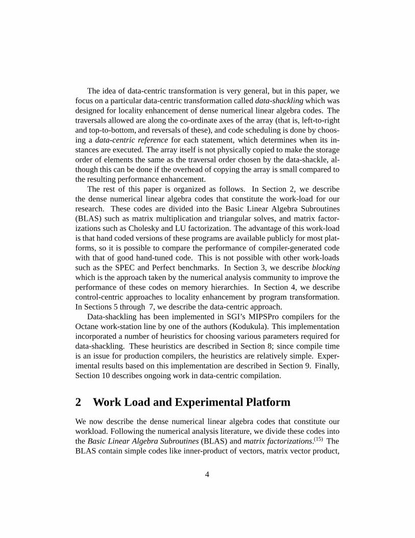
The idea of data-centric transformation is very general, but in this paper, wefocus on a particular data-centric transformation called data-shackling which wasdesigned for locality enhancement of dense numerical linear algebra codes. Thetraversals allowed are along the co-ordinate axes of the array (that is, left-to-rightand top-to-bottom, and reversals of these), and code scheduling is done by choos-ing a data-centric reference for each statement, which determines when its in-stances are executed. The array itself is not physically copied to make the storageorder of elements the same as the traversal order chosen by the data-shackle, al-though this can be done if the overhead of copying the array is small compared tothe resulting performance enhancement.

The rest of this paper is organized as follows. In Section 2, we describethe dense numerical linear algebra codes that constitute the work-load for ourresearch. These codes are divided into the Basic Linear Algebra Subroutines(BLAS) such as matrix multiplication and triangular solves, and matrix factor-izations such as Cholesky and LU factorization. The advantage of this work-loadis that hand coded versions of these programs are available publicly for most plat-forms, so it is possible to compare the performance of compiler-generated codewith that of good hand-tuned code. This is not possible with other work-loadssuch as the SPEC and Perfect benchmarks. In Section 3, we describe blockingwhich is the approach taken by the numerical analysis community to improve theperformance of these codes on memory hierarchies. In Section 4, we describecontrol-centric approaches to locality enhancement by program transformation.In Sections 5 through 7, we describe the data-centric approach.

Data-shackling has been implemented in SGI’s MIPSPro compilers for theOctane work-station line by one of the authors (Kodukula). This implementationincorporated a number of heuristics for choosing various parameters required fordata-shackling. These heuristics are described in Section 8; since compile timeis an issue for production compilers, the heuristics are relatively simple. Exper-imental results based on this implementation are described in Section 9. Finally,Section 10 describes ongoing work in data-centric compilation.

2 Work Load and Experimental Platform

We now describe the dense numerical linear algebra codes that constitute ourworkload. Following the numerical analysis literature, we divide these codes intothe Basic Linear Algebra Subroutines (BLAS) and matrix factorizations.(15) TheBLAS contain simple codes like inner-product of vectors, matrix vector product,

4

Table I: Behavior of some BLAS

Operation Data Touched Computation Algorithmic reuse Levelz � � � x� y O�n� O�n� x� y� z: O��� 1A � x O�n�� O�n�� x: O�n�, A: O��� 2C � C � A �B O�n�� O�n�� A�B�C: O�n� 3

triangular solve, and matrix matrix multiplication. The important matrix factor-izations are Cholesky, LU and QR factorizations. We also describe the hardwareon which all experiments were performed.

2.1 Basic Linear Algebra Subroutines

The following five operations occur frequently in applications.(15)

� Dot product: Given two column vectors x and y, computes the inner productxTy.

� Saxpy: Given a scalar � and column vectors x and y, computes the columnvector z equal to � � x� y.

� Matrix Vector Product: Given an m � n matrix A and a column vector x,computes y � A � x.

� Triangular solve: Given a square lower triangular matrix L with non-zerodiagonal elements and a column vector b, solve the system Lx � b.

� Matrix Multiplication: Given an m� p matrix A, an p� n matrix B and anm� n matrix C, computes C � C � A �B.

Figure 1 shows pseudo-code for each of these core routines.Three important properties of each of these core routines are (i) amount of

data touched, (ii) the number of floating point operations, and (iii) the averageamount of data reuse (which is the ratio of the two previous quantities). Table Isummarizes this information for each of the core operations.

The information in Table I provides a guide to the potential performance ofBLAS on a machine with a memory hierarchy. Dot product, called a Level-1BLAS, performs � � n floating-point operations on � � n data elements. On the

5

sum = 0do i = 1, nsum += x(i) * y(i)

do i = 1, nz(i) += � * x(i) + y(i)

(a) Inner (dot) Product (b) Scalar * x + y (Saxpy)

do i = 1, mdo j = 1, n

y(i) += A(i,j) * x(j)

do i = 1, nx(i) = b(i)do j = 1, i-1x(i) = x(i) - L(i,j)*x(j)

x(i) = x(i)/L(i,i)

(c) Matrix Vector Product (d) Triangular solve

do i = 1, mdo j = 1, ndo k = 1, pC(i,j) += A(i,k) * B(k,j)

(e) Matrix Multiplication

Figure 1: Basic Linear Algebra Subroutines

6

average, one data item must be touched for each floating-point operation that isperformed, so there is little reuse of data even in the algorithm. The characteristicsof saxpy are similar. Matrix vector product performs ��n� operations on n����ndata, so the amount of data touched per floating-point operation is half of thatin the case of Level-1 BLAS. There is no reuse of matrix elements but each ofthe vectors exhibits O�n� amount of reuse. Matrix vector product and triangularsolve are called Level-2 BLAS. Finally, matrix multiplication performs O�n��operations on O�n�� data and is called a Level-3 BLAS operation. Clearly, thereis significant algorithmic reuse of data in matrix multiplication, and exploiting thisreuse is the key to good performance on a machine with a memory hierarchy.

2.2 Matrix factorizations

We will consider the following matrix factorization codes: (i) Cholesky factoriza-tion, (ii) LU factorization, and (iii) QR factorization.

2.2.1 Cholesky factorization

Cholesky factorization is used to solve the system of equations Ax = b, whereA is a symmetric positive-definite matrix, by factorizing A into the product LLT,where L is lower-triangular, and solving the two resulting triangular systems. Tosave space, the lower triangular part of A is overwritten with the factor L.

Cholesky factorization, like matrix multiplication, has three nested loops al-though these loops are imperfectly nested. All six permutations of these loopsare legal, and distributing the loops in one of these versions gives a total of sevenversions of Cholesky factorization that we discuss in this paper. Pseudocode forone of these versions is shown in Figure 2; pseudocode for the other versions areshown in Figure 18 through 24.

The most commonly described version is the so-called kij version (alsoknown as the right-looking version), and it is shown in Figure 2. This versionprocesses the columns of the matrix in left to right order as follows: the squareroot of the diagonal element of the current column is computed, the portion ofthis column below the diagonal is scaled with this value and the outer-product ofthis portion of the column with its transpose is used to update the lower triangularportion of the matrix to the right of the current column. These are known as thesquare root, scale and update steps respectively. For obvious reasons, this versionof Cholesky factorization is also known as right-looking column Cholesky factor-ization. Distributing the i loop over the scale step and the update loop produces

7

do k = 1, nS1: A(k,k) = sqrt (A(k,k)) //square root stepdo i = k+1, n

S2: A(i,k) = A(i,k) / A(k,k) //scale stepdo j = k+1, iS3: A(i,j) -= A(i,k) * A(j,k) //update step

Figure 2: kij-fused version of Cholesky factorization

another kij version of Cholesky factorization, shown in Figure 18. Permutingthe two update loops in the code of Figure 18 gives the kji version shown inFigure 20.

Right-looking Cholesky factorization performs updates eagerly in the sensethat the columns to the right of the current column are updated as soon as thatcolumn is computed. An alternative is to perform the updates lazily, which meansthat a column is updated only when it becomes current. This leads to the left-looking column Cholesky factorization code (also called the jki version) shownin Figure 22 which applies updates from all columns to the left of the currentcolumn before performing the square root and scaling steps. Permuting the i andk loops gives the jik version shown in Figure 21.

Finally, there are two versions of Cholesky factorization called the ijk andikj versions that process the matrix by row rather than by column. These areshown in Figures 23 and 24. The ijk version performs inner-products, so it isalso known as dot Cholesky while the ikj version in contrast is rich in saxpyoperations.

2.2.2 LU factorization

LU factorization is used to solve linear systems when the matrix is not guaran-teed to be symmetric positive definite. To improve the stability of this process, anoperation called partial pivoting is performed during the factorization. LU fac-torization, like Cholesky factorization and matrix multiplication, has three nestedloops that may be permuted to produce a number of versions. One version of LUfactorization is shown in Figure 3. The k loop, which is outermost, walks overthe columns of the matrix. In each iteration of this loop, the entries in column kbelow the diagonal of the matrix are examined, and the row that contains the ele-ment of largest magnitude is determined (call it row m). If m and k are distinct, the

8

portion of row of k to the right of the diagonal is swapped with the correspondingportion of row m (this is called partial pivoting). Scale and update steps are thenperformed as in Cholesky factorization, but the update is applied to the sub-matrixbelow and to the right of the diagonal element A(k,k). Note that the i and jloops in the update step can be interchanged, giving rise to two different versionsof LU factorization with pivoting.

This version of LU factorization is called right-looking LU factorization. Asin the case of Cholesky factorization, there are two left-looking versions in whichupdates to a column are delayed until that column becomes current. Interactionsbetween updates and pivoting are sufficiently complex that there is no direct ana-log of row Cholesky factorization for LU factorization with pivoting. It is possibleto perform LU factorization row by row, but this code must do column pivoting,and is therefore a different algorithm than the left- and right-looking column ver-sions. We do not consider this version in this paper.

2.2.3 QR factorization

QR factorization, shown in Figure 4 is used in eigenvalue computations, and itfactorizes A into a product Q*R where Q is an orthonormal matrix and R is uppertriangular. The Householder variant of QR factorization proceeds through the ma-trix A column by column. For each column, a Householder vector is determinedsuch that when the corresponding Householder reflection is applied, the portionof the current column strictly below the diagonal contains only zeros. For a vectorx, if e� represents the unit vector with a � in the first entry, and zeros in all otherentries, v � �x�kxk��e���k�x�kxk��e��k represents a unit-length Householdervector such that on applying a Householder reflection to x, all entries except thefirst are zeroed out. Once a Householder vector v has been determined for thecurrent column, a Householder reflection can be applied to the rest of the matrix.Conceptually, a Householder reflection can be thought of as multiplying the restof the matrix by �I��vvT �, which would take O�n�� operations for v of length n.However, this reflection can actually be accomplished in O�n�� operations by us-ing a two-step process. The key observation is that for a matrix B, �I� �vvT ��B= B� �v � vT �B = B� �v �w, where w � vT �B. Thus the first step computesw using a matrix vector computation and the second step updates the rest of thematrix using an outer product update computation.

9

do k = 1, ntemp = 0.0d0m = k//find pivot rowdo i = k, nd = A(i,k)if (ABS (d) .gt. temp)temp = abs(d)m = i

if (m .ne. k)ipvt(k) = m//row permutationdo j = k, ntemp = A(k,j)A(k,j) = A(ipvt(k),j)A(ipvt(k),j) = temp

//scale loopdo i = k+1, nA(i,k) = A(i,k) / A(k,k)

//update loopsdo i = k+1, ndo j = k+1, nA(i,j) -= A(i,k) * A(k,j)

Figure 3: kij version of LU with pivoting

10

do k = 1, nnorm = 0do i = k, n

norm = norm + A(i,k) * A(i,k)norm2 = dsqrt (norm)asqr = A(k,k) * A(k,k)A(k,k) =

dsqrt(norm-asqr+((A(k,k)-norm2)�))//Householder vector computationdo i = k+1, nA(i,k) = A(i,k) / A(k,k)

//Reflection - (matrix vector product)do i = k+1, nw(i) = 0do j = i, nw(i) += A(j,i) * A(j,k)

//Reflection - (outer product update)do j = k+1, ndo i = k+1, nA(i,j) = A(i,j) - 2 * A(i,k) * w(j)

Figure 4: QR factorization

11

2.3 Hardware Platform

The experimental results reported in this paper were obtained on an unloaded Oc-tane workstation with an R10000 processor running at 195 MHz. The R10K canperform one load/store operation and two floating point operations per cycle, giv-ing it a theoretical peak performance of 390 MFlops. The processor has 32 logicalregisters and 64 physical registers. The workstation was equipped with separatefirst-level (L1) instruction and data caches of size 32Kb each, and a second-level(L2) unified cache of size 1MB. The L1 cache is non-blocking with a miss penaltyof 10 cycles, and it is organized as a 2-way set associative cache with a line sizeof 32 bytes. The L2 cache is also non-blocking with a miss penalty of 70 cycles,and it is organized as a 2-way set associative cache with a line size of 128 bytes.Therefore, the four highest levels of memory hierarchy are the registers, the L1and L2 caches and main memory.

3 Library Approaches

In this section, we discuss the approach taken by the numerical linear algebracommunity to produce high-performance codes for the work-load described inSection 2, and argue that it is difficult for a restructuring compiler to mimic thisapproach directly.

The numerical linear algebra community has taken a layered approach to theproblem of implementing portable, high-performance code for matrix applica-tions.

1. Machine-specific code is written for each of the BLAS. These codes are notportable since the performance optimizations in these codes are machine-specific.

2. Matrix factorizations are expressed as block algorithms rather than as pointalgorithms. The restructuring of point algorithms to block algorithms ex-poses BLAS-3 like matrix multiplication and triangular solve with multiplerighthand sides which are executed by invoking machine-specific BLAS.This is the approach followed in the LAPACK library.(2)

The upshot of this strategy is that only the BLAS are not portable; the matrixfactorization codes are layered on top of the BLAS, and are machine-independent.

12

do t1 = 1 .. d� n����edo t2 = 1 .. d� n����edo t3 = 1 .. d� n����edo It = (t1-1)*25 +1 ..

min(t1*25,n)do Jt = (t2-1)*25 +1 ..

min(t2*25,n)do Kt = (t3-1)*25 +1 ..

min(t3*25,n)C(It,Jt) = C(It,Jt) + A(It,Kt) * B(Kt,Jt)

C

B

A

Figure 5: Blocked Code for matrix matrix multiplication

3.1 BLAS routines

We use matrix multiplication to discuss how the BLAS are implemented. Thenaive version in Figure 1(e) does not exploit data reuse effectively; for example,for every iteration of the outermost loop, the matrix B is read in its entirety. Ifthe matrices are much larger than the cache, none of the reuse of B is exploited.The solution is to use a block algorithm that performs a sequence of small matrixmultiplications, each of which multiplies a submatrix of A with a submatrix ofB, accumulating the result in a submatrix of C, as shown in Figure 5. If thesesubmatrices are small enough to fit into the cache, the number of capacity missesdecreases substantially.

How big the submatrices should be clearly depends on the size of the cacheand is therefore machine-specific, but it can conveyed as a parameter to the blockcode. The need for machine-specific code arises because a good code for matrixmultiplication must pay careful attention to register allocation of array elements.If the k loop is innermost in the submatrix multiplication code, C(i,j) can beheld in a register, reducing the number of loads and stores in each inner loop it-eration by 2. This can improve performance for two reasons: (i) register accessesare faster than cache accesses, and (ii) most microprocessors have a small num-ber of pipes to memory, so having many loads and stores in an inner loop canthrottle the performance of the processor pipeline. On the other hand, it is alsoadvantageous to have the i and j loops innermost since B(k,j) and A(i,k)respectively become invariant in the innermost loop, and can be read once andstored in a register. The solution to these conflicting demands is to register tile thesubmatrix multiplication itself, and choose the size of the tiles so that array values

13

300.0 400.0 500.0 600.0 700.0Problem Size

0.0

100.0

200.0

300.0

400.0

Meg

aflo

ps

Performance of handwritten BLAS librarySGI Octane Workstation

Matrix Matrix multiplication (Level–3)Matrix Vector Product (Level–2)Saxpy (Level–1)

Figure 6: Performance of computations from Levels 1, 2 & 3

can be read and written in registers in the innermost loop. In addition to registertiling, the innermost loop must be software pipelined to reduce the effect of loadlatencies. These considerations mandate the use of very machine-specific code inwriting high-performance BLAS.

Detailed information regarding the implementation of BLAS on a modernhigh-performance computer can be found in.(1) Figure 6 shows the performanceof handcoded BLAS on the SGI Octane. These routines were implemented byMimi Celes at SGI.

3.2 Block matrix factorizations

From Figure 6, it is easy to see that the point versions of matrix factorization codeswill perform poorly on a machine with a memory hierarchy. For example, in thekij version of Cholesky factorization shown in Figure 2, the innermost loop per-forms a saxpy operation (notice that A(i,k) is invariant in this loop, and its valueis used to scale a portion of the kth column of A which is then added to a portionof the ith row of A). Since BLAS-1 operations perform poorly on a memory hi-erarchy, we would expect that this point version of Cholesky factorization wouldperform poorly as well. This is in fact the case, as we show in Section 9. Fortu-nately, it is possible to restructure the computation to expose BLAS-3 operations.To illustrate this, we show that the block algorithm in the LAPACK library can bederived from the point version by program restructuring.

14

do k = 1, ndo i = k, ndo j = k, iif (i == k && j == k) A(k,k) = sqrt (A(k,k));if (i > k && j == k) A(i,k) = A(i,k) / A(k,k);if (i > k && j > k) A(i,j) -= A(i,k) * A(j,k);

Figure 7: A fully permutable loop nest for Cholesky factorization

do js = 0, n/B //this counts the block columnsdo i = B*js +1, ndo k = 1, min(i,B*js+B)do j = max(B*js +1,k), min(i,B*js+B)

if (i == k && j == k) A(k,k) = sqrt (A(k,k));if (i > k && j == k) A(i,k) = A(i,k) / A(k,k);if (i > k && j > k) A(i,j) -= A(i,k) * A(j,k);

Figure 8: Stripmine-and-interchange of code in Figure 7

It can be shown that the perfectly nested loop shown in Figure 7 performsCholesky factorization, and that the three loops are fully permutable. This per-fectly nested version of Cholesky factorization can be generated from the kij-fusedversion shown in Figure 2 by repeated application of code-sinking.(35)

The first step in generating the block-j version of Cholesky used in the LA-PACK library is to stripmine the j loop in blocks of size B, and interchange loopsto produce the code shown in Figure 8.

Next, we simplify the loop bounds to get rid of min’s and max’s by index-setsplitting the i and k loops. The index-set of the i loop is split into two rangesB*js+1 to B*js+B, and B*js+B+1 to n. The index set of the k loop is splitinto the two ranges 1 to B*js, and B*js+1 to i. Simplifying the predicatesthen gives us the code shown in Figure 9. A pictorial representation of this codeis shown in Figure 10.

To get good performance, the matrix multiplications and triangular solve mustbe performed by calling the appropriate BLAS.

Similar block algorithms can be derived for LU with pivoting and QR factor-ization. For LU with pivoting, the block algorithm in LAPACK exploits the factthat row permutations commute with updates, while the block QR factorization

15

do js = 0, n/B

//Computation 1: matrix multiplicationdo i= B*js +1, B*js+Bdo k = 1,B*jsdo j = B*js +1,iA(i,j) -= A(i,k) * A(j,k);

//Computation 2: small Cholesky factorizationdo i = B*js +1,B*js+Bdo k = B*js+1,ido j = k,iif (i == k && j == k) A(k,k) = sqrt (A(k,k));if (i > k && j == k) A(i,k) = A(i,k) / A(k,k);if (i > k && j > k) A(i,j) -= A(i,k) * A(j,k);

//Computation 3: matrix multiplicationdo i = B*js+B+1,ndo k = 1,B*jsdo j = B*js+1,B*js+BA(i,j) -= A(i,k) * A(j,k);

//Computation 4: triangular solve with multiple RHSdo i = B*js+B+1,ndo k = B*js+1,B*js+Bdo j = k,B*js+B

if (j == k) A(i,k) = A(i,k) / A(k,k);if (j > k) A(i,j) -= A(i,k) * A(j,k);

Figure 9: Index-set splitting of code in Figure 8

16

����������������������������������������

����������������������������������������

������������

������������

���������������

���������������

���������������

��������������� 2

4

1

3

block

Computation 1: MMMComputation 2: unblocked CholeskyComputation 3: MMMComputation 4: Triangular solve

column

j

k

i

A

Figure 10: Pictorial view of code in Figure 9

350.0 550.0 750.0 950.0Problem Size (nxn matrix)

0.0

50.0

100.0

150.0

200.0

250.0

300.0

350.0

MF

lops

Cholesky FactorizationQR Factorization (Block Householder Reflection)LU Factorization with Pivoting

Figure 11: Performance of Cholesky, QR & LU Factorization codes from LA-PACK

exploits associativity of matrix products.The performance of LAPACK factorization codes on the SGI Octane is shown

in Figure 11. Cholesky factorization runs at roughly 250 MFlops while QR andLU with pivoting run at roughly 200 MFlops.

17

3.3 Discussion

It is seems unlikely that a compiler can mimic the steps outlined above for de-riving block Cholesky code from point Cholesky. Transforming the kij-fusedversion of Cholesky factorization into the fully permutable loop nest of Figure 7by code sinking is reasonably straight-forward, but it should be noted that thereare many ways to apply code sinking to the program in Figure 2, and each ofthese produces different perfectly nested loops. For example, in Figure 7, thesquare root and scale steps can be done when (j == k+1) without changingthe semantics of the program. Moreover, generating the perfectly nested versionfrom other versions of Cholesky factorization is non-trivial. In the kji versionfor example, the j and i loops must be interchanged, then the two i loops mustbe fused, after which code sinking can be applied to generate the fully permutableversion. It is not clear what would drive a compiler to make these choices.

Once the perfectly nested loop is generated, another sequence of transfor-mations is required to extract the BLAS-3 sub-computations from the fully per-mutable loop nest. As before, it is not clear how one might automate this sequenceof transformations.

The approach of restructuring code to expose BLAS-3 operations and exe-cuting these operations using machine-tuned BLAS has been used successfullyto produce high-performance library code, but we believe that it is difficult for acompiler to imitate this strategy directly.

4 Existing Compiler Approaches

The compiler community has developed many techniques for enhancing localityby restructuring perfectly nested loops. In contrast, much less is known aboutlocality enhancement in imperfectly nested loops.

4.1 Perfectly nested loops

The most effective transformation is loop tiling, preceded if necessary by linearloop transformations like permutation and skewing.(5, 19, 21, 35) For example, con-sider a nested loop that adds the elements of a two-dimensional array stored incolumn-major order. If the code is written so that the array is accessed by row,spatial locality is enhanced by permuting the loops so that the innermost loopwalks over the array with unit stride. This example demonstrates the use of lin-

18

ear loop transformations for locality enhancement, but it does not require tiling.In codes like matrix multiplication, locality can improved by moving any one ofseveral loops into the innermost position, as discussed in Section 3.1. Tiling isbeneficial for such codes since it gives the effect of interleaving the iterations ofthese loops, thereby providing most of the benefits of having all these loops inthe innermost position. Matrix multiplication therefore demonstrates the need fortiling. Tiling is not always legal, so the most general strategy is to apply linearloop transformations to convert a loop nest into a fully permutable loop nest whichcan be tiled. A critical parameter in tiling a loop nest is tile size which must bechosen so that cache misses are as small as possible during the execution of thetile. Many heuristics for choosing good tile sizes have been developed.(6, 13, 14)

A very sophisticated implementation of these techniques can be found in theSGI MIPSPro compiler for the Octane workstation.(33) This compiler convertssingly nested loop nests into perfectly nested loop nests using code sinking, andthen tiles the resulting perfectly nested loop nest.

Definition 4.1.1 A singly nested loop (SNL) is an imperfectly nested loop in whichthere is at most one loop nested immediately inside every loop.

The triangular solve code in Figure 1 and the kij-fused version of Choleskyfactorization in Figure 2 are SNL’s while the kij version of the Cholesky factor-ization code in Figure 18 is an example of an imperfectly nested loop that is notan SNL. All the BLAS codes are SNL’s, so the SGI MIPSPro compiler achievesgood performance on these code, as can be seen in Figure 12. The performance ofthe compiled code is roughly equal to that of handwritten code for BLAS-1 andBLAS-2; for BLAS-3, the handwritten version is moderately better. The structureof the compiled code for BLAS-3 is identical to that of the handwritten code, butthe handwritten version does a better job of choosing block sizes.

4.2 Imperfectly nested loops

Matrix factorization codes are imperfectly nested and only the kij-fused ver-sion of Cholesky factorization is an SNL.

The MIPSPro compiler attempts to perform loop transformations like fusionand distribution to transform these codes into perfectly nested loops that canbe tiled, but it is successful in doing this only for the kij-fused version ofCholesky factorization. Therefore, the performance of compiled code for matrixfactorizations is quite poor, as we discuss in detail in Section 9.

19

300.0 400.0 500.0 600.0 700.0Problem Size

0.0

100.0

200.0

300.0

400.0

500.0

Meg

aflo

ps

DGEMM in BLAS-3Compiler-transformed matrix-matrix multiplyCompiler-transformed matrix-Vector multiplyDGEMV in BLAS-2DAXPY in BLAS-1Compiler-transformed a*x + y

Figure 12: Performance of handwritten and compiled BLAS

A number of approaches for enhancing locality in imperfectly nested loopshave been proposed in the research literature. Carr and Kennedy analyzed blockfactorizations such as Cholesky and LU, and showed that sequences of loop trans-formations such as index-set splitting, loop distribution and stripmine-and-interchangecan produce blocked codes from unblocked ones.(7) This is like the approach wetook in Section 3, but it does not require conversion to a fully permutable, perfectlynested loop nest as an intermediate step since imperfectly nested loop transforma-tions such as index-set splitting are applied directly. However, it is not clear whatwould drive a compiler to synthesize such sequences of transformations. In addi-tion, their work considered only the kij version of Cholesky factorization; otherversions of Cholesky factorization require different sequences of transformations.To block LU factorization with pivoting, they propose to introduce pattern match-ing into the compiler to permit it to recognize that row permutation commuteswith updates. This work was extended by Carr and Lehoucq(9) to QR factoriza-tion, although the blocked version they developed is different from the one inLAPACK.

Ramanujam and Schreiber(29) used a combination of code sinking and loopfusion to convert some of the imperfectly nested variants of Cholesky to the fullypermutable, perfectly nested intermediate form of Figure 7. Their strategy workswell for the kij and kij-fused versions of Cholesky factorization, but it can-not be applied to other versions because loop fusion is not legal in these codes.

McKinley et al(23) present a cost model for memory accesses and use it to

20

determine the best version of Cholesky factorization, but they do not considertiling.

More recently, Song and Li developed a technique for tiling imperfectly nestedloops that arise in relaxation codes.(30) However, this technique is very specific torelaxation codes, and cannot be used to improve locality in matrix factorizationcodes for example.

5 Data-centric Transformation

We now describe data-shackling, a locality enhancement technique designed tobe applicable to imperfectly nested loops. In data-shackling, the compiler picksan order in which data structure elements should be brought into the cache atruntime, and it restructures code so that statement instances that access a givenelement are scheduled close together in time. When the transformed program isexecuted, data structure elements will be brought into the cache in approximatelythe order chosen by the compiler. In this way, the locality enhancement problemis converted to a scheduling problem in which the schedule of statement executionis matched to the schedule of data movement chosen by the compiler.

5.1 Data-shackling

The key concept in data-shackling is the idea of a data-shackle.

Definition 5.1.1 A data-shackle is a specification in three parts.

1. One of the arrays in the program is divided into blocks using sets of parallel,equally spaced cutting planes. Each set of cutting planes is specified by anorientation and a pitch.

2. An order for visiting the blocks of data is specified.

3. One reference to that array is selected for each statement in the program.This reference is called the data-centric reference for that statement.

Intuitively, the data-shackle specifies an order in which blocks of the arrayare touched, and the data-centric reference is used to determine which iterationsof each statement get performed when that block of the array is touched — codeis generated to perform all iterations of that statement for which the data-centricreference touches data within the current block.

21

N

N

0 1 2 3

0

2

<1,1> <1,2> <1,3> <1,4>

<2,1> <2,2> <2,3> <2,4>

<3,1> <3,2> <3,3> <3,4>

3

1

<4,1> <4,2> <4,3> <4,4>

do b1 = 1 .. d�N����edo b2 = 1 .. d�N����edo i = 1 .. Ndo j = 1 .. Ndo k = 1 .. Nif ((b1-1)*25 < i <= b1*25) &&

((b2-1)*25 < j <= b2*25)C(i,j) = C(i,j) + A(i,k) * B(k,j)

(a) Blocking of C matrix (b) Naive code produced by shackling C

do t1 = 1 .. d�N����edo t2 = 1 .. d�N����edo i = (t1-1)*25 +1 ..

min(t1*25,N)do j = (t2-1)*25 +1 ..

min(t2*25,N)do k = 1 .. NC(i,j) = C(i,j) + A(i,k) * B(k,j)

A

B

CK

K

(c) Simplified code produced by IP tool (d) Data touched by code

Figure 13: Code produced by shackling C in matrix-multiply

We illustrate this with matrix multiplication. One data-shackle is obtained bydividing C into 2-dimensional 25x25 blocks using horizontal and vertical sets ofcutting planes, as shown in Figure 13(a). These blocks can be visited in left-to-right, top-to-bottom order. C(i,j) is the only reference to this array in theassignment statement, and it is chosen to be the data-centric reference for thatstatement.

Figure 13(b) shows naive code generated by using this data-shackle. There aretwo outermost loops which enumerate over the blocks of C. For each block, theentire initial loop nest is executed, and two conditionals are inserted at the inner-most level to ensure that the data touched by the data-centric reference lies withinthe current block. This code generation strategy is reminiscent of the runtimeresolution code generation strategy which is used in compiling shared-memoryprograms for distributed-memory machines.(27) This code is shown only to illus-

22

trate the high-level idea of a data-shackle. In the implementation, standard integerlinear programming tools are used to fold the bounds of the data blocks into theinner loop bounds, producing the optimized code shown in Figure 13(c). Noticethat within the context of a single block, iterations are done in the same order asin the original code (these are called intra-block iterations), but in the program asa whole, the order in which iterations are performed is different from their orderin the source program. Therefore, shackling is not always legal. In Section 6, weshow that the determination of whether a data-shackle is legal can be reduced tothe standard problem of determining the emptiness of the union of certain polyhe-dra, a problem for which many algorithms exist.

This shackle does not produce the standard block matrix multiplication codediscussed in Section 2.1. For a given block of C, the data-shackle specified aboveconstrains the i and j loop indices, but does not constrain the k index in any way,as can be seen in Figure 13(d). This results in poor locality for the A(i,k) andB(k,j) references. This problem can be addressed by composing shackles, asexplained in Section 7.

A more complicated example is data-shackling of the kij-fused versionof Cholesky factorization. The array A can be blocked into 64x64 blocks in amanner similar to Figure 13(a). When a block is scheduled, all statements thatwrite to that block can be executed in program order. In other words, the referencechosen from each statement of the loop nest is the left hand side reference in thatstatement. The code obtained after simplification with polyhedral algebra toolsis shown in Figure 14. The reader who wants some insight into the structureof this code should study Figure 15. data-shackling regroups the iteration spaceinto four sections. Initially, all updates to the diagonal block from the left areperformed (Figure 15(i)). This is followed by a small Cholesky factorization(15)

of the diagonal block (Figure 15(ii)). For each off-diagonal block, updates fromthe left (Figure 15(iii)) are followed by interleaved scaling of the columns of theblock by the diagonal block, and local updates(Figure 15(iv)).

As in the case of matrix multiplication, this code is only partially blocked,compared to the block factorization code in the LAPACK library. Although allthe writes are performed into a block when that block is visited, reads are notlocalized to blocks but are distributed over the entire left portion of the matrix. Aswith matrix multiplication, this problem is solved by composing shackles.

23

Source code:do k = 1, nS1: A(k,k) = dsqrt (A(k,k))do i = k+1, nS2: A(i,k) = A(i,k) / A(k,k)

do i = k+1, ndo j = k+1, iS3: A(i,j) -= A(i,k) * A(j,k)

Shackled code:do t1 = 1, (n+63)/64/* Apply updates from left to diagonal block */do t3 = 1, 64*t1-64do t6 = 64*t1-63, min(n,64*t1)do t7 = t6, min(n,64*t1)A(t7,t6) = A(t7,t6) - A(t7,t3) * A(t6,t3)

/* Cholesky factor diagonal block */do t3 = 64*t1-63, min(64*t1,n)A(t3,t3) = sqrt(A(t3, t3))do t5 = t3+1, min(64*t1,n)A(t5,t3) = A(t5,t3)/ A(t3,t3)

do t6 = t3+1, min(n,64*t1)do t7 = t6, min(n,64*t1)A(t7,t6) = A(t7,t6) - A(t7,t3) * A(t6,t3)

/* Apply updates from left tooff-diagonal block */

do t2 = t1+1, (n+63)/64do t3 = 1, 64*t1-64do t6 = 64*t1-63, 64*t1do t7 = 64*t2-63, min(n,64*t2)A(t7,t6) = A(t7,t6) - A(t7,t3) * A(t6,t3)

/* Apply internal scale/updates tooff-diagonal block */

do t3 = 64*t1-63, 64*t1do t5 = 64*t2-63, min(64*t2,n)A(t5,t3) = A(t5,t3)/ A(t3,t3)

do t6 = t3+1, 64*t1do t7 = 64*t2-63, min(n,64*t2)A(t7,t6) = A(t7,t6) - A(t7,t3) * A(t6,t3)

Figure 14: Data-shackling applied to right-looking Cholesky factorization

24

(iv) Internal scale+update (iii) Update off-diagonal block from left

(ii) Cholesky factor diagonal block(i) Update diagonal block from left

t3 t6

t7

t3

t5

t3 t6

t7

t3

t5

t6

Figure 15: Pictorial View of Code in Figure 14

5.2 Discussion

By shackling a data reference R in a source program statement S, we ensure thatthe memory access made from that data reference at any point in program execu-tion will be constrained to the “current” data block. Turning this around, we seethat when a block becomes current, we perform all instances of statement S forwhich the reference R accesses data in that block. Therefore, this reference enjoysperfect self-temporal locality.(32) Considering all shackled references together, wesee that we also have perfect group-temporal locality for this set of references; ofcourse, references outside this set may not necessarily enjoy group-temporal local-ity with respect to this set. As mentioned earlier, we do not mandate any particularorder in which the data points within a block are visited. However, if all dimen-sions of the array are blocked and the block fits in cache (or whatever level of thememory hierarchy is under consideration), we obviously exploit spatial locality,regardless of whether the array is stored in column-major or row-major order. Aninteresting observation is that if stride-1 accesses are mandated for a particularreference, we can simply use cutting planes with unit separation which enumeratethe elements of the array in storage order. Enforcing stride-1 accesses within theblocks of a particular blocking can be accomplished by composing shackles asdescribed in Section 7.

The code shown in Figure 14 can certainly be obtained by a (long) sequence of

25

traditional iteration space transformations like sinking, tiling, index-set splitting,distribution etc. As we discussed in the introduction, it is not clear for imperfectlynested loops in general how a compiler determines which transformations to carryout and in what sequence these transformations should be performed.

6 Legality of Data Shackling

Since data-shackling reorders statement instances, we must ensure that it doesnot violate dependences. An instance of a statement S can be identified by avector i which specifies the values of the index variables of the loops surroundingS. The tuple (S,i) represents instance i of statement S. Suppose there is adependence from (S1,i1) to (S2,i2) and suppose that these two instancesare executed when blocks b� and b� are touched respectively. For the data-shackleto be legal, either b� must be touched before b�, or b� and b� must be identical(note that if b� and b� are identical, the code generation strategy in Section 5ensures that the statement instances are executed in original program order). Inthis case, we say that the data-shackle respects that dependence. A data-shackleis legal if it respects all dependences in the program. Since our techniques applyto imperfectly nested loops like Cholesky factorization, it is not possible to usedependence abstractions like distance and direction to verify legality. Instead, wesolve integer linear programming problems, as we discuss in this section.

6.1 An example of testing legality

To understand the general algorithm, it is useful to consider first a simple exampledistilled from the Cholesky factorization code of Figure 14. In the source code,there is a flow dependence from the assignment of A(k,k) in S1 to the use ofA(k,k) in S2. We must ensure that this dependence is respected in the shackledcode shown in Figure 14.

We first write down a set of integer inequalities that represents the existenceof a flow dependence between an instance of S1 and an instance of S2. Let S1write to an array location in iteration kw of the k loop, and let S2 read from thatlocation in iteration �kr� ir� of the k and i loops. A flow dependence exists if thefollowing linear inequalities have an integer solution:(35)

26

���������������

kr � kw (same location)

n � kw � � (loop bounds)

n � kr � � (loop bounds)

n � ir � kr � � (loop bounds)

kr � kw (read after write)

(1)

Next, we assume that the instance of S1 is performed when a block �b��� b���is scheduled, and the instance of S2 is done when block �b��� b��� is scheduled.Finally, we add a condition that represents the condition that the dependence isviolated in the transformed code. In other words, we formulate the condition thatblock �b��� b��� is touched strictly before block �b��� b���. These conditions arerepresented as: ���������������

��������������

Writing iteration done in (b��� b��)

b�� � ��� �� � kw � b�� � ��

b�� � ��� �� � kw � b�� � ��

Reading iteration done in (b��� b��)

b�� � ��� �� � kr � b�� � ��

b�� � ��� �� � ir � b�� � ��

Blocks visited in bad order

�b�� � b��� � ��b�� � b��� � �b�� � b����

(2)

If the conjunction of the two sets of conditions (1) and (2) has an integersolution, it means that there is a dependence, and that dependent instances areperformed in the wrong order. If so, the data-shackle violates the dependence andis not legal. This problem can be viewed geometrically as asking whether theunion of certain polyhedra contains an integer point. This problem can be solvedusing standard polyhedral algebra tools.

Such a test can be performed for each dependence in the program. If no de-pendences are violated, the data-shackle is legal.

6.2 General View of Legal Data-Shackles

The formulation of the general problem of testing for legality of a data-shackle be-comes simpler if we first generalize the notion of blocking data. A data blocking

27

xx xx

x xxx

xx xx

x xxx

(S2,I2)

(S1,I1)

GenerationCode

Original Program Transformed Program

Data with new co-ordinatesOriginal Data

C

A

T

V

Figure 16: Testing for Legality

such as the one shown in Figure 13(a) can be viewed simply as a map that assignsco-ordinates in some new space to every data element in the array. For example, ifthe block size in this figure is 25 x 25, array element �a�� a�� is mapped to the co-ordinate ���a� � �� div ��� � �� ��a� � �� div ��� � �� in a new two-dimensionalspace. Note that this map is not one-to-one. The bottom part of Figure 16 showssuch a map pictorially. The new space is totally ordered under lexicographic or-dering. The data shackle can be viewed as traversing the remapped data in lexico-graphic order in the new co-ordinates; when it visits a point in the new space, allstatement instances mapped to that point are performed.

Therefore, a data-shackle can be viewed as a function M that maps statementinstances to a totally ordered set (V, �). For the blocking shown in Figure 16,C:(S,I) A maps statement instances to elements of array A through data-centric references, and T:A V maps array elements to block co-ordinates.Concisely, M = TC.

Given a function M:(S,I)(V,�), the transformed code is obtained bytraversing V in increasing order, and for each element v � V, executing the state-ment instances M��(v) in program order in the original program.

Theorem 6.2.1 A map M:(S,I) (V,�) generates legal code if the follow-ing condition is satisfied for every pair of dependent statements S1 and S2.

� Introduce vectors of unknowns i1 and i2 that represent instances of de-

28

pendent statements S1 and S2 respectively.

� Formulate the inequalities that must be satisfied for a dependence to existfrom instance i1 of statement S1 to instance i2 of statement S2. This isstandard.(35)

� Formulate the predicate M(S2,i2)�M(S1,i1).

� The conjunction of these conditions does not have an integer solution.

Proof: Obvious, hence omitted. �

6.3 Discussion

Viewing blocking as a remapping of data co-ordinates simplifies the developmentof the legality test. This remapping is merely an abstract mathematical device toenforce a desired order of traversal through the array, and the physical array itselfis not necessarily reshaped. For example, in the blocked matrix multiplicationcode in Figure 13, array C need not be laid out in block order to obtain the benefitsof blocking this array. This is similar to the situation in BLAS/LAPACK whereit is assumed that the FORTRAN column-major order is used to store arrays. Ofcourse, nothing prevents us from reshaping the physical data array if the cost ofconverting back and forth from a standard representation is tolerable. Automaticdata reshaping has been explored by other researchers.(3, 11)

7 Products of shackles

We now show that there is a natural notion of taking the Cartesian product of a setof shackles, and that this notion is the data-centric equivalent of loop nesting.

The motivation for this operation comes from the matrix multiplication codeof Figure 13(c), in which an entire block row of A is multiplied with a block ofcolumn of B to produce a block of C. The order in which the iterations of thiscomputation are done is left unspecified by the data-shackle (the default codegeneration scheme of Section 5 will execute these iterations in original programorder). Note that the shackle on reference C(I,J) constrains both I and J,but leaves K unconstrained; therefore, the references A(I,K) and B(K,J) cantouch an unbounded amount of data in arbitrary ways during the execution of theiterations shackled to a block of C(I,J)). Instead of C, we can block A or B,

29

but this still results in unconstrained references to the other two arrays. To getBLAS-style blocked matrix multiplication, we need to block all three arrays. Weshow that this effect can be achieved by taking Cartesian products.

Informally, the notion of taking the Cartesian product of two shackles canbe viewed as follows. The first shackle partitions the statement instances of theoriginal program, and imposes an order on these partitions. However, it does notmandate an order in which the statement instances in a given partition shouldbe performed. The second shackle refines each of these partitions separately intosmaller, ordered partitions, without reordering statement instances in different par-titions obtained from the first shackle. In other words, if two statement instancesare ordered by the first shackle, they are not reordered by the second shackle. Thenotion of a binary Cartesian product can be extended the usual way to an n-aryCartesian product; each extra factor in the Cartesian product gives us finer controlover the granularity of data accesses.

A formal definition of the Cartesian product of data-shackles is the following.Recall from the discussion in Section 6 that a data-shackle for a program P can beviewed as a map M:(S,I) V, whose domain is the set of statement instancesand whose range is a totally ordered set.

Definition 7.0.1 For any program P, let�M� � �S� I� V�

M� � �S� I� V�

be two data-shackles. The Cartesian productM� �M� of these shackles is de-fined as the map whose domain is the set of statement instances, whose range isthe Cartesian product V� � V� and whose values are defined as follows: for anystatement instance (S,i), �M� �M���S� i� � �M��S� i��M��S� i� �

The product domain V��V� of two totally ordered sets is itself a totally orderedset under standard lexicographic order. Therefore, the code generation strategyand associated legality condition are identical to those in Section 6. It is easy tosee that for each point v� � v� in the product domain V� � V�, we perform thestatement instances in the set �M� �M��

���v�� v�� �M����v�� �M�

���v��.In the implementation, each term in an n-ary Cartesian product contributes a

guard around each statement. The conjunction of these guards determines whichstatement instances are performed at each step of execution. Therefore, theseguards still consist of conjuncts of affine constraints. As with single data-shackles,the guards can be simplified using any polyhedral algebra tool.

30

Note that the product of two shackles is always legal if the two shackles are le-gal by themselves. However, a productM��M� can be legal even ifM� by itselfis illegal. This is analogous to the situation in loop nests where a loop nest may belegal even if there is an inner loop that cannot be moved to the outermost position;the outer loop in the loop nest “carries” the dependence that causes difficulty forthe inner loop.

7.1 Examples

In matrix multiplication, it is easy to see that shackling any of the three refer-ences (C(I,J),A(I,K),B(K,J)) to the appropriate blocked array is legal.Therefore, all Cartesian products of these shackles are also legal. The Carte-sian product MC �MA of the C and A shackles produces the code in Figure5. It is interesting to note that further shackling with the B shackle (that is theproduct MC �MA �MB) does not change the code that is produced. This isbecause shackling C(I,J) to the blocks of C and shackling A(I,K) to blocksof A imposes constraints on the reference B(K,J) as well. A similar effect canbe achieved by shackling the references C(I,J) and B(K,J), or A(I,K) andB(K,J).

A more interesting example is the Cholesky code. In Figure 2, it is easy to ver-ify that there are six ways to shackle references in the source program to blocks ofthe matrix (choosing A(K,K) from statement S1, either A(I,K) or A(K,K)from statement S2 and either A(I,J), A(I,K) or A(J,K) from statementS3). Of these, only two are legal: choosing A(K,K) from S1, A(I,K) fromS2 and A(I,J) from S3, or choosing A(K,K) from S1, A(K,K) from S2 andA(I,K) from S3. The first shackle chooses references that write to the block,while the second shackle chooses references that read from the block. Since boththese shackles are legal, their Cartesian product (in either order) is legal. It canbe shown that one order gives a fully-blocked left-looking Cholesky, similar tothe blocked Cholesky algorithm in LAPACK, while the other order gives a fully-blocked right-looking Cholesky. The left-looking code produced by shackling isshown in Figure 27.

7.2 Discussion

Taking the Cartesian product of data-shackles gives us finer control over data ac-cesses in the blocked code. As discussed earlier, shackling just one referencein matrix multiplication (say C(I,J)) does not constrain all the data accesses.

31

On the other hand, shackling all three references in this code is over-kill sinceshackling any two references constraints the third automatically. Taking a largerCartesian product than is necessary does not affect the correctness of the code, butit introduces unnecessary loops into the resulting code which must be optimizedaway by the code generation process to get good code. In Section 8, we explainhow our implementation of data-shackling determines when to stop composingdata-shackles.

8 Heuristics used in Implementation

Sections 5, 6 and 7 described the mechanisms that underlie data shackling. Animplementation of data-shackling must make certain policy decisions as well. Oneof the authors (Kodukula) has implemented data-shackling in the SGI MIPSProcompiler. In this section, we describe the policies implemented in this compiler. Ina production compiler, the time taken to compile programs must be kept small, sothese policies are based on heuristic choices that are simple to implement. Theireffectiveness for our workload is discussed in Section 9. We believe that ourheuristics are reasonable, although it is certainly easy to invent other plausibleones.

8.1 Policy decisions

An implementation of shackling must address the following questions.

1. What is the program unit to which data-shackling is applied?

2. How are the parameters for a single data-shackle chosen?

(a) Which array is shackled?

(b) What is the orientation of the cutting planes?

(c) What is the order of traversal of blocks?

(d) What is the separation of cutting planes (block sizes)?

(e) How are data-centric references chosen?

3. How many shackles are composed?

32

One approach to answering many of these questions is to treat them as classi-cal optimization problems, and try to find optimal solutions in the context of anaccurate model. However, this approach is impractical in a production compiler,so we developed heuristics instead.

8.2 Program unit for shackling

Shackling is applied to one imperfectly nested loop at a time. Shackling is es-sentially statement scheduling, so it can be applied in principle to multiple im-perfectly nested loops or even to entire programs, but we do not have enoughexperience at this point to do this effectively.

8.3 Determining the parameters of a single shackle

We now describe the decisions that must be made to determine a single data-shackle.

Picking an array for the shackle: Arrays are ordered by the following criteria.

� What is the largest row rank of a data access matrix2 of an unconstrainedreference to the array?

� How many unconstrained references of this rank are there?

� Has the array already been used in a shackle?

If two or more arrays are tied according to one criterion, we attempt to breakthe tie using succeeding criteria. If there are multiple choices at the end of thisprocess, the tie is broken arbitrarily. The rationale for this heuristic is that an arrayto which there are multiple unconstrained references of large rank is likely to be amajor participant in cache traffic.

For example, in Figure 17, array A is given highest priority for shackling be-cause there are two unconstrained references of row-rank two to this array. Notethat array B has only one reference of rank two, while array s has three references,all of rank one.

2If all array access functions are linear functions of loop variables (if the functions are affine,the constant terms can be dropped), an array access function can be written as F � I where F isthe data access matrix(20) and I is the vector of iteration space variables of loops surrounding thisdata reference.

33

do i = 1, ndo j = 1, mS1: s(i) = A(i,2*j+1)S2: r = 9.1 + jS3: A(i,2*j) += s(i)*s(i) + rS4: A(i,2*j) += r + B(i,j)

Figure 17: Choosing an array for shackling

Orientation of cutting planes: Cutting plane orientations are always chosen tobe parallel to the data co-ordinate axes. Dongarra and Schreiber have explored theuse of skewed blocks for locality enhancement,(14) but skewed blocks are likelyto produce variable trip-count inner loops which are detrimental to subsequentphases in the compiler such as software pipelining (the MIPSPro compiler doesnot use loop skewing for the same reason).

Order of traversal of blocks: An n-dimensional array is blocked by choosing nsets of cutting planes; for example, a two-dimensional array is blocked along bothrows and columns. The order of traversal of blocks is chosen to be a lexicographicorder on block co-ordinates. For a two-dimensional array, the blocks are visitedfrom left to right, and within a given block column, from top to bottom. If thisorder is not legal, the compiler tries a right to left order, and also a bottom to toporder. If none of these four orders of traversal is legal, the compiler tries to blockonly rows or only columns. If that fails as well, the imperfectly nested loop is notshackled.

Choice of data-centric references: Picking a data-centric reference for eachstatement is a two step process. In the first step, all candidate data-centric ref-erences for a statement are determined. The second step is simply an exhaustiveenumeration of all candidate data-centric references for each statement, searchingfor a legal shackle. We focus on the first step in the following discussion.

After an array has been picked for a shackle, data-centric references to thisarray must be selected for each statement. At the one extreme, candidate refer-ences for a statement could be limited to references to the array that actually occurin that statement. This causes difficulties in programs like the one in Figure 17because statement S2 does not contain a reference to array A which is the arraychosen for shackling. At the other extreme, all references to the shackled array inthe entire imperfectly nested loop can be candidate references for every statement,

34

but this may result in a combinatorial explosion in the number of possibilities thatmust be considered.

Our implementation chooses an intermediate position which is easy to under-stand by considering the program in Figure 17. There is a flow dependence fromstatement S2 to S3 because S2writes to the scalar variable rwhile S3 reads fromit. This dependence may not be respected if the data-centric references chosen forthe two statements are different (for example, if the data-centric reference for S2is A(i,2j+1) and the data-centric reference for S3 is A(i,2j)). Therefore,candidate data-centric references for S2 should be candidates for S4 and viceversa.

Our implementation therefore divides statements into equivalence classes suchthat two statements are in the same equivalence class if and only if there is adependence between them that is induced by a scalar or an array that will not beshackled. For example, if there are dependences from S1 to S2 and from S1 toS3, all three statements are placed in the same equivalence class even if there isno dependence from S2 to S3. The candidate references for a statement are allreferences to the shackled array that occur in the statements in its equivalenceclass. For the program in Figure 17 for example, all statements will be placed inthe same equivalence class, so all array references in the loop will be candidatereferences for all statements.

Our implementation then tries each candidate reference for each statement,and checks if the resulting program is legal. If legality is violated because ofa dependence due to a scalar, our implementation performs scalar expansion toeliminate the problem. Array expansion of low-dimensional array that cause thisproblem is possible in principle, but we have not implemented this.

Finally, we mention that all assignment statements within a conditional state-ment are placed in the same equivalence class because they are all control depen-dent on the predicate.

Block Size Determination: To determine block sizes, we used a simplifiedversion of the algorithm used in the MIPSPro compiler for determining tile sizeswhen it tiles perfectly nested loops. This algorithm estimates the amount of datatouched in computing a tile (this is called the footprint of the tile), and choosesa tile size such that this footprint is a certain fraction of the cache size called theeffective cache size (between 5 and 10%). It might appear that cache misses areminimized when the effective cache size is equal to the cache size, but experiencehas shown that the use of a smaller effective cache size reduces conflict misseswithout much impact on capacity misses.

35

We adapted this model to shackling by computing the block size at whichthe footprint of the intra-block iterations of the shackled code was equal to theeffective cache size. The computation of this footprint was done as follows.

In the first step, a set of references with large contributions to the footprintare identified in each statement. For statements that are not most deeply nestedin the imperfectly nested loop, this set is defined to be empty. For statementsthat are most deeply nested, this set is defined to be all the references from thatstatement with the highest (row)-ranked access matrices. For example, in matrixmultiplication, A(i,k), B(k,j) and C(i,j) all correspond to access matricesof row-rank 2, and are all chosen in this step. In Cholesky factorization, theupdate statement is most deeply nested, and the three references chosen from itare A(i,j), A(i,k) and A(j,k).

The second step performs the following computations for each statement. Thereferences chosen in the previous step are partitioned into groups — two refer-ences to the same array fall into the same group if their access matrices havethe same linear part, but possibly different affine parts. References belongingto two different arrays always fall into different groups. For example, in ma-trix multiplication, A(i,k), B(k,j) and C(i,j) all fall into different groups.Similarly, in Cholesky factorization, A(i,j), A(i,k) and A(j,k) fall intodifferent groups. On the other hand, two references of the form A(i,j) andA(i+1,j) will be assigned to the same group. The assumption is that all refer-ences assigned to the same group enjoy perfect reuse, while references assigned todifferent groups enjoy no reuse. Finally, two groups from two different statementsreferring to the same array are merged if the references in the two groups have thesame linear part, and the two statements under consideration have identical data-centric references. The assumption is that if the data-centric references for the twostatements are identical, instances of the two statements that touch the same datawill be scheduled close enough together that they will enjoy perfect reuse. If Erepresents the effective size of the cache and g represents the number of groups,then each group is allowed to have a footprint as large as E�g.

The last step involves computing the footprint of every group for a single in-stance of a composite shackle. Two simplifications are applied to this computation— (i) the footprint of a group is approximated by the footprint of a single refer-ence picked at random from the group, and (ii) it is assumed that the footprint ofthe group is identical for all instances of the data loops introduced by the shackle.The first simplification is justified by the assumption that all references in a groupenjoy perfect reuse, and the second simplification is justified since boundary ef-fects are not significant when array sizes and loop bounds are large. The reference

36

picked for each group is called the representative reference.Evaluating the footprint of a single reference for the intrablock iterations of

shackled code is straightforward, and variations of this problem have been ad-dressed in the literature.(24) A single instance of the composite shackle is com-pletely specified by a specific set of values for the block coordinates for each levelof a composite shackle - for the sake of simplicity, each of the block coordinatescan be assumed to be . In addition, we only consider square blocks, so for everyarray a, a single unknown parameter Ba denotes the block size for that array. Asystem of linear integer equations expressing the localization constraints corre-sponding to the composite shackle is assembled for the statement containing therepresentative reference. The number of distinct elements touched by the rep-resentative reference under this system of equations is multiplied by the size ofeach element to yield a polynomial in a single parameter for the footprint for thisreference. Determining the number of distinct elements touched by the represen-tative reference is thus reduced to the problem of counting the number of integersinside a convex polyhedron. In our current implementation, this is estimated bycounting the number of integer solutions inside the bounding box of the convexpolyhedron. More sophisticated approaches such as Ehrhart Polynomials(12) canpotentially be used to obtain better solutions in practice, but it is not clear whetherthis improvement in accuracy leads to better overall performance.

We implemented shackling only to improve performance of the L2 cache; themiss latency for the L1 cache is small enough that we decided not to shackle forthe L1 cache. Therefore, block sizes were determined using the size of the L2cache.

8.4 How many shackles are composed?

Composing data-shackles provides finer control over data accesses in the blockedcode. As discussed earlier, shackling just one reference in matrix multiplication(say C(i,j)) does not constrain all the data accesses. On the other hand, shack-ling all three references in this code is over-kill since shackling any two referencesconstraints the third automatically. Applying too many levels of composition doesnot affect the correctness of the code, but it introduces unnecessary loops into theresulting code which must be optimized away by the code generation process toget good code. The following obvious result is useful to determine how far tocarry the process of taking Cartesian products.

37

Theorem 8.4.1 For a given statement S, let F�� � � � � Fn be the access matricesfor the shackled data references in this statement. Let Fn�� be the access matrixfor an unshackled reference in S. Assume that the data accessed by the shackledreferences are bounded by block size parameters. Then the data accessed by Fn��is bounded by block size parameters iff every row of Fn�� is spanned by the rowsof F�� � � � � Fn.

Stronger versions of this result can be proved, but it sufficed for purposes ofthe implementation. For example, the access matrix for the reference C(i,j)

is

�� �

�. Shackling this reference does not bound the data accessed by

row� �

�of the access matrix

� � �

�of reference B(k,j). How-

ever, taking the Cartesian product of this shackle with the shackle obtained fromA(i,k) constrains the data accessed by B(k,j), because all rows of the corre-sponding access matrix are spanned by the set of rows from the access matricesof C(i,j) and A(i,k). Composition is applied if even a single assignmentstatement from the loop nest under consideration stands to benefit as a result.

8.5 Discussion

Once all shackles have been determined, localization constraints must be foldedinto loop bounds (for example, we must generate the code shown in Figure 13(c)rather than the code in Figure 13(b)). This code generation step has been imple-mented in polyhedral algebra tools like PIP and Omega. Our implementation usesa simple version of these techniques to generate the shackled code quickly. Theinterested reader is referred to Kodukula’s thesis.(17)

9 Experiments

We present experimental results showing the performance of different versionsof Cholesky, LU and QR factorizations. The performance of compiler-generatedBLAS codes was shown in Figure 12.

9.1 Cholesky factorization

Like matrix multiplication, Cholesky factorization has three nested loops, butthese loops are imperfectly nested. All six permutations of these three loops are

38

do k = 1, nA(k,k) = dsqrt (A(k,k))do i = k+1, nA(i,k) = A(i,k) / A(k,k)

do i = k+1, ndo j = k+1, iA(i,j) -= A(i,k) * A(j,k) 500 600 700 800 900 1000 1100

Problem Size

0.0

100.0

200.0

300.0

Cum

ulat

ive

Meg

aflo

ps

Cache/Register optimizations turned offBenefit from Shackling/Tiling for L2Additional benefit from Register Tiling

(a) Source code (b) Performance of tiled and shackled codes

400.0 600.0 800.0 1000.0 1200.0 1400.0Problem Size

0.0

50.0

100.0

150.0

200.0

250.0

300.0

MF

lops

10305060708090110

0

0.5

1

1.5

2

2.5

3

3.5

4

500 600 700 800 900 1000 1100

Cac

he M

iss

Rat

io (

%)

Problem Size

TilingShackling

(c) Effect of varying block size (d) L2 miss ratios for tiled and shackled codes

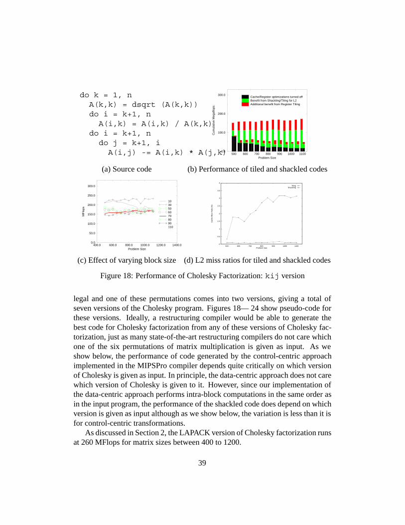
Figure 18: Performance of Cholesky Factorization: kij version

legal and one of these permutations comes into two versions, giving a total ofseven versions of the Cholesky program. Figures 18— 24 show pseudo-code forthese versions. Ideally, a restructuring compiler would be able to generate thebest code for Cholesky factorization from any of these versions of Cholesky fac-torization, just as many state-of-the-art restructuring compilers do not care whichone of the six permutations of matrix multiplication is given as input. As weshow below, the performance of code generated by the control-centric approachimplemented in the MIPSPro compiler depends quite critically on which versionof Cholesky is given as input. In principle, the data-centric approach does not carewhich version of Cholesky is given to it. However, since our implementation ofthe data-centric approach performs intra-block computations in the same order asin the input program, the performance of the shackled code does depend on whichversion is given as input although as we show below, the variation is less than it isfor control-centric transformations.

As discussed in Section 2, the LAPACK version of Cholesky factorization runsat 260 MFlops for matrix sizes between 400 to 1200.

39

do k = 1, nA(k,k) = dsqrt (A(k,k))do i = k+1, nA(i,k) = A(i,k) / A(k,k)do j = k+1, iA(i,j) -= A(i,k) * A(j,k)

500 600 700 800 900 1000 1100Problem Size

0.0

100.0

200.0

300.0

Cum

ulat

ive

Meg

aflo

ps

Cache/Register optimizations turned offBenefit from Shackling/Tiling for L2Additional benefit from Register Tiling

(a) Source code (b) Performance of tiled and shackled codes

400.0 600.0 800.0 1000.0 1200.0 1400.0Problem Size

0.0

50.0

100.0

150.0

200.0

250.0

300.0

MF

lops

10305060708090110

0

0.05

0.1

0.15

0.2

0.25

0.3

500 600 700 800 900 1000 1100

Cac

he M

iss

Rat

io (

%)

Problem Size

TilingShackling

(c) Effect of varying block size (d) L2 miss ratios for tiled and shackled codes

Figure 19: Performance of Cholesky factorization: kij-fused version

We implemented shackling only to improve performance of the L2 cache; themiss latency for the L1 cache is small enough that we decided not to shackle forthe L1 cache. The shackled code produced by the compiler was generated bycomposing two shackles. In both shackles, the array was divided into rectangularblocks (the compiler heuristic chose 70x70 blocks), and these blocks were vis-ited in left-to-right, top-to-bottom order. In the outer shackle, the compiler chosethe left-hand side reference from each assignment statement for shackling, whilein the inner shackle, the compiler selected a reference from the right-hand sideof each statement: A(k,k) for the square root statement, and A(i,k) for thescale and update statements. The same shackle was used for all other versions ofCholesky factorization as well.

The shackled code performs better than the tiled code in both versions of kijCholesky, as shown in Figures 18 and 19. Figure 18(d) shows that the miss ratiofor the tiled code increases rapidly with array size, showing that tiling in the SGIcompiler is not effective; in contrast, the miss ratio of the shackled code is almostindependent of array size. The kij-fused version in Figure 19 is an SNL, so

40

do k = 1, nA(k,k) = dsqrt (A(k,k))do i = k+1, nA(i,k) = A(i,k) / A(k,k)

do j = k+1, ndo i = j, nA(i,j) -= A(i,k) * A(j,k) 500 600 700 800 900 1000 1100

Problem Size

0.0

100.0

200.0

300.0

Cum

ulat

ive

Meg

aflo

ps

Cache/Register optimizations turned offBenefit from Shackling/Tiling for L2Additional benefit from Register Tiling

(a) Source code (b) Performance of tiled and shackled codes

400.0 600.0 800.0 1000.0 1200.0 1400.0Problem Size

0.0

50.0

100.0

150.0

200.0

250.0

300.0

MF

lops

10305060708090110

0

0.5

1

1.5

2

2.5

3

500 600 700 800 900 1000 1100

Cac

he M

iss

Rat

io (

%)

Problem Size

TilingShackling

(c) Effect of varying block size (d) L2 miss ratios for tiled and shackled codes

Figure 20: Performance of Cholesky Factorization: kji version

41

do j = 1, ndo i = j, ndo k = 1, j-1A(i,j) -= A(i,k) * A(j,k)

A(j,j) = dsqrt (A(j,j))do i = j+1, nA(i,j) = A(i,j) / A(j,j) 500 600 700 800 900 1000 1100

Problem Size

0.0

100.0

200.0

300.0

Cum

ulat

ive

Meg

aflo

ps

No L2 Shackling and no Register TilingBenefit from Shackling for L2Additional benefit from Register Tiling

(a) Source code (b) Performance of tiled and shackled codes

400.0 600.0 800.0 1000.0 1200.0 1400.0Problem Size

0.0

50.0

100.0

150.0

200.0

250.0

300.0

MF

lops

10305060708090110

0

1

2

3

4

5

500 600 700 800 900 1000 1100

Cac

he M

iss

Rat

io (

%)

Problem Size

TilingShackling

(c) Effect of varying block size (d) L2 miss ratios for tiled and shackled codes

Figure 21: Performance of Cholesky Factorization: jik version

the SGI compiler is more successful in enhancing locality in this version. Thesefigures also show the relative contributions of shackling (for the L2 cache) and ofregister tiling to overall performance. With neither of these locality optimizations,the performance of the baseline code drops to about 10-20 MFlops! Register tilingeliminates many loads and stores of array locations and boosts the performance ofthe shackled code from 110 MFlops to 175 MFlops. This is consistent with otherreports in the literature about the importance of register tiling.(8)

Figures 18(c) and 19(c) show the effect of varying the block size in the shack-led code. It can be seen the optimal block size is 30 x 30 rather than the 70 x70 chosen by the compiler. With this block size, the performance of the shack-led code is boosted to 240 Mflops which is very close to LAPACK performance.These figures suggest that the heuristic for choosing block sizes needs to be im-proved.

Permuting the two update loops in the kij version gives the kji versionshown in Figure 20. This version is not an SNL, so tiling is not effective. Fusingthe scale loop with the outer update loop is illegal. The only way to get an SNL is

42

do j = 1, ndo k = 1, j-1do i = j, nA(i,j) -= A(i,k) * A(j,k)

A(j,j) = dsqrt (A(j,j))do i = j+1, nA(i,j) = A(i,j) / A(j,j) 500 600 700 800 900 1000 1100

Problem Size

0.0

100.0

200.0

300.0

Cum

ulat

ive

Meg

aflo

ps

Cache/Register optimizations turned offBenefit from Shackling/Tiling for L2Additional benefit from Register Tiling

(a) Source code (b) Performance of tiled and shackled codes

400.0 600.0 800.0 1000.0 1200.0 1400.0Problem Size

0.0

50.0

100.0

150.0

200.0

250.0

300.0

MF

lops

10305060708090110

0

1

2

3

4

5

6

500 600 700 800 900 1000 1100

Cac

he M

iss

Rat

io (

%)

Problem Size

TilingShackling

(c) Effect of varying block size (d) L2 miss ratios for tiled and shackled codes

Figure 22: Performance of Cholesky Factorization: jki version

43

do i = 1, ndo j = 1, i-1do k = 1, j-1A(i,j) -= A(i,k) * A(j,k)

A(i,j) = A(i,j)/A(j,j)do k = 1, i-1

A(i,i) -= A(i,k) * A(i,k)A(i,i) = dsqrt (A(i,i))

500 600 700 800 900 1000 1100Problem Size

0.0

100.0

200.0

300.0

Cum

ulat

ive

Meg

aflo

ps

Cache/Register optimizations turned offBenefit from Shackling/Tiling for L2Additional benefit from Register Tiling

(a) Source code (b) Performance of tiled and shackled codes

400.0 600.0 800.0 1000.0 1200.0 1400.0Problem Size

0.0

50.0

100.0

150.0

200.0

250.0

300.0

MF

lops

10305060708090110

0

1

2

3

4

5

6

7

500 600 700 800 900 1000 1100

Cac

he M

iss

Rat

io (

%)

Problem Size

TilingShackling

(c) Effect of varying block size (d) L2 miss ratios for tiled and shackled codes

Figure 23: Performance of Cholesky Factorization: ijk version

44

do i = 1, ndo k = 1, i-1A(i,k) = A(i,k) / A(k,k)do j = k+1, iA(i,j) -= A(i,k) * A(j,k)

A(i,i) = dsqrt (A(i,i))500 600 700 800 900 1000 1100

Problem Size

0.0

100.0

200.0

300.0

Cum

ulat

ive

Meg

aflo

ps

Cache/Register optimizations turned offBenefit from Shackling/Tiling for L2Additional benefit from Register Tiling

(a) Source code (b) Performance of tiled and shackled codes

400.0 600.0 800.0 1000.0 1200.0 1400.0Problem Size

0.0

50.0

100.0

150.0

200.0

250.0

300.0

MF

lops

10305060708090110

0

1

2

3

4

5

500 600 700 800 900 1000 1100

Cac

he M

iss

Rat

io (

%)

Problem Size

TilingShackling

(c) Effect of varying block size (d) L2 miss ratios for tiled and shackled codes

Figure 24: Cholesky Factorization: ikj version

to interchange the two update loops and then fuse the new outer update loop withthe scale loop, generating the code of Figure 19, but this is too complicated for theMIPSPro compiler’s imperfectly nested loop transformation heuristics to reasonabout. Therefore, cache tiling has little benefit as is evident in Figure 20(b). Theperformance of the baseline code (no cache or register tiling) is modestly betterthan that of the baseline kij versions because of better spatial locality in theupdate loops. This also explains why the shackled code performs a little betterthan the shackled code from the kij version.

Figure 21 shows the performance of a left-looking version of Cholesky factor-ization. The loop nest is not an SNL, but the computational work in the updateloops is essentially a matrix-vector product which is performed by the MIPSProcompiler by accumulating the updates to A(i,j) in a register. The shackled ver-sion exploits reuse at all loop levels and outperforms the tiled code substantiallyexcept when the array size is around 950. This sudden drop in performance iscaused by conflict misses. Figure 21(c) shows that choosing the block size adap-tively to reduce conflict misses is one solution. However, the current implemen-

45

tation of shackling does not choose block sizes adaptively. In the jik version,all the updates to an element of the current column are performed before succeed-ing elements are updated. Permuting the i and k loops gives the jki version.The MIPSPro compiler interchanges the update loops in the jki back to the jikversion, so the performance of the baseline and tiled versions is identical to theperformance of the jik versions. There is no difference in the performance ofthe shackled code either.

Finally, Figures 23 and 24 show the performance of row-Cholesky versions.The ijk version performs inner-products, so it is also known as ddot Choleskywhile the ikj version is rich in saxpy operations. Figure 23(b) shows that whilethe shackled code outperforms the tiled code, it performs poorly compared toLAPACK code. To understand why, note that Figure 23(d) shows that the L2 cachemiss ratios are similar to those of Figure 18, but Figure 24(b) shows that registertiling is not effective in this code. The shackled code for the ikj version performsbetter, but it too appears exploits register tiling to a limited extent. Improving theperformance of the ikj and ijk versions requires closer integration of shacklingwith register tiling.

9.2 LU factorization

Figure 25 compares the performance of shackling and tiling for LU factorizationwith pivoting. As mentioned before, the entire loop nest is not an SNL, and there-fore cannot be tiled. However, the update loop nest can be tiled, and this has asmall benefit because it permits spatial locality to be exploited.

Using simple data-flow analysis, it can be determined that for the LU factor-ization code in Figure 25, the scalar m needs to be expanded. The data shacklechosen by the compiler divides array A into block columns with block sizes rang-ing from 10 to 25 depending on the size of the problem. For the scale and up-date statements, the shackling references are chosen to be A(i,k) and A(j,l)respectively. For the three statements implementing the row permutations, theshackling references are A(k,j), A(k,j) and A(ipvt(k),j) respectively,and for all the other statements, the shackling reference is A(i,k). We finallynote that in this particular example, the expansion of m can be completely free,since ipvt(k) represents precisely a scalar expanded m; however this analysisis not currently implemented.

While the performance of the shackled code beats the performance of the tiledcode, it is still slower than the LAPACK version by a factor of 2. This is becausethe LAPACK code uses information about the commutativity of permutations and

46

250.0 450.0 650.0 850.0Size of matrix (NxN)

0.0

100.0

200.0

MF

lops

Shackled versionTiled versionUntiled version

Figure 25: LU Factorization with Partial Pivoting

row-updates; this permits it in essence to use two-dimensional blocking ratherthan block columns, which results in better code. Restructuring based on depen-dence analysis does not change the order of writes to a given memory location, sowe believe that it is unlikely that a compiler that uses dependence analysis alonecan deduce this commutativity condition automatically. We have recently shownthat fractal symbolic analysis can solve this problem.(22)

9.3 QR factorization

QR factorization performs orthogonal factorization of a matrix A into the productQR where Q is an orthonormal matrix and R is upper triangular. It is a key kernelin eigenvalue calculations. Figure 26 compares the performance of shackling andtiling on QR factorization using Householder reflections.(15) As in the case of LUfactorization with partial pivoting, the array A is partitioned into block columnsbecause a two-dimensional blocking is not legal. QR is similar to LU factorizationexcept that in this case, array expansion of the vector x is required for legality.The necessary array expansion has not yet been implemented, so we modified thestandard code for QR factorization to perform array expansion. Figure 26 showsthis program. The need to expand x raises an important profitability question -scalar expansion is usually quite cheap, however expanding x creates an array aslarge as A in this case. Although shackling once again outperforms tiling, theperformance of the shackled code is a factor of 2 worse than that of the LAPACK

47

200.0 400.0 600.0Size of matrix (NxN)

0.0

100.0

200.0

MF

lops

Shackled versionTiled versionUntiled version

Figure 26: QR Factorization using Householder reflections

code which obtains roughly 225 MFlops on this code. The LAPACK code usesa number of deep properties of matrices, such as associativity of matrix product,to generate efficient code. It is conceivable that a compiler could exploit some ofthis information if the input program were written in a language like MATLAB orFORTRAN-90 in which array operations are primitives.

10 Conclusions and Future Work

In this paper, we introduced the data-centric approach to optimizing scientificprograms to improve cache performance, described an implementation of this ap-proach within the SGI MIPSPro compiler, and compared the performance of data-centric code with that of code generated by more conventional control-centrictechniques.

The key insight behind the data-centric approach is that it is often easier fora compiler to perform locality-enhancing transformations if it reasons about datastructure traversals rather than control structure transformations. Intuitively, thecompiler determines a schedule for the arrival of data structure elements in thecache, determines what computations should be performed when that data arrives,and generates the appropriate code. At runtime, program execution will automati-cally pull data into the cache in roughly that order, and the hit ratio should improvebecause statements that touch the same data are scheduled together.

48

We discussed a particular implementation of the data-centric approach calleddata-shackling which was designed for locality enhancement of dense numericallinear algebra codes. The traversals allowed are along the co-ordinate axes ofthe array (that is, left-to-right and top-to-bottom, and reversals of these); for eachstatement, a data-centric reference is chosen heuristically which determines theinstances of that statement that are executed when a given data structure elementis brought into the cache. The array itself is not physically copied to make the stor-age order of elements the same as the traversal order chosen by the data-shackle,although this can be done if it is deemed to be profitable.

This work can be extended in many ways.As the experimental results in Section 9 show, data-shackling does not gen-

erate code competitive with LAPACK library code for LU factorization with piv-oting and QR factorization. The blocked code in the LAPACK library for LUfactorization with pivoting exploits the fact that row permutations commute withupdates (see the code in Figure 3). A compiler that uses dependence analysis pre-serves the order of reads and writes to a given memory location in the originalprogram, so better analysis techniques must be developed. We have recently in-vented a technique called fractal symbolic analysis that addresses this problem(22)

but its use in automatic locality enhancement remains to be explored. BlockingQR factorization requires the exploitation of domain-specific information like theassociativity of matrix multiplication, and it is not clear how a compiler could begiven such information or how it would use such information.

Our current implementation does not change the storage order of blocks ofthe array to make it the same as the traversal order chosen by the data-shackle,but nothing prevents us from reshaping the physical data array if the cost of con-verting back and forth from a standard representation is tolerable. Automatic datareshaping has been explored by other researchers,(3, 11) and it would be interestingto see what benefits this would have in our context.

Data-centric transformations other than data-shackling need to be explored.For example, Pugh and Rosser have proposed a data-centric transformation callediteration space slicing(25) which can be viewed as a more systematic way of us-ing dependences than the heuristics described in Section 8 for finding data-centricreferences. A backward slice for a variable at a given point in the program isthe portion of the program that affects the value of that variable at that programpoint.(31) Given an order in which array elements are to be computed, iterationspace slicing produces a program that is effectively the sequence of incremen-tal slices of successive elements of the array. However, computing incrementalslices is computationally expensive, and the performance advantage over simple

49

heuristics is unclear.Finally, large computational science problems usually involve sparse matrices

produced by the applications of methods like the finite-element method. Sparsematrix programs cannot be restructured or optimized by compilers because arrayaccesses in these programs involve indirect subscripts that are difficult for a com-piler to reason about. We have shown that this problem can be circumvented byusing the data-centric approach to synthesize sparse matrix programs from densematrix programs and specifications of sparse formats.(18) The sparse format isspecified in part by describing efficient traversal orders for enumerating the ele-ments of the matrix, and the restructuring compiler attempts to use one of thesedata element traversal orders to perform the specified computation.

50

Acknowledgements: Nawaaz Ahmed participated in some of the early workon data-shackling. Dror Maydan and Robert Cox helped with the SGI implemen-tation of data shackling. Rob Schreiber and Charlie van Loan explained many ofthe LAPACK algorithms to us. Finally, Nikolai Mateev, Vijay Menon and PaulStodghill gave us valuable feedback on this paper.

References

[1] Ramesh C. Agarwal and Fred G. Gustavson. Algorithm and ArchitectureAspects of Producing ESSL BLAS on POWER2.

[2] E. Anderson, Z. Bai, C. Bischof, J. Demmel, J. Dongarra, J. DuCroz, A. Greenbaum, S. Hammarling, A. McKenney, S. Ostrouchov, andD. Sorensen, editors. LAPACK Users’ Guide. Second Edition. SIAM,Philadelphia, 1995.

[3] Jennifer Anderson, Saman Amarsinghe, and Monica Lam. Data and com-putation transformations for multiprocessors. In ACM Symposium on Prin-ciples and Practice of Parallel Programming, Jun 1995.

[4] U. Banerjee. Unimodular transformations of double loops. In Proceedingsof the Workshop on Advances in Languages and Compilers for Parallel Pro-cessing, pages 192–219, August 1990.

[5] Uptal Banerjee. Unimodular transformations of double loops. In Languagesand compilers for parallel computing, pages 192–219, 1990.

[6] Pierre Boulet, Alain Darte, Tanguy Risset, and Yves Robert. (Pen)-ultimatetiling? In INTEGRATION, the VLSI Journal, volume 17, pages 33–51. 1994.

[7] Steve Carr and K. Kennedy. Compiler blockability of numerical algorithms.In Supercomputing, 1992.

[8] Steve Carr and R. B. Lehoucq. Compiler blockability of dense matrix fac-torizations. Technical report, Argonne National Laboratory, Oct 1996.

[9] Steven Carr and R. B. Lehoucq. A compiler-blockable algorithm for QRdecomposition, 1994.

51

[10] L. Carter, J. Ferrante, and S. Flynn Hummel. Hierarchical tiling for improvedsuperscalar performance. In International Parallel Processing Symposium,April 1995.

[11] Michael Cierniak and Wei Li. Unifying data and control transformationsfor distributed shared memory machines. In SIGPLAN 1995 conference onProgramming Languages Design and Implementation, Jun 1995.

[12] Philippe Clauss. Counting solutions to linear and nonlinear constraintsthrough ehrhart polynomials: Applications to analyze and transform scien-tific programs. In ACM Int. Conf. on Supercomputing. ACM, May 1996.

[13] Stephanie Coleman and Kathryn S. McKinley. Tile size selection usingcache organization and data layout. In ACM SIGPLAN ’95 Conference onProgramming Language Design and Implementation (PLDI). ACM Press,June 1995.

[14] Jack Dongarra and Robert Schreiber. Automatic blocking of nested loops.Technical Report UT-CS-90-108, Department of Computer Science, Univer-sity of Tennessee, May 1990.

[15] Gene Golub and Charles Van Loan. Matrix Computations. The Johns Hop-kins University Press, 1996.

[16] F. Irigoin and R. Triolet. Supernode partitioning. In ACM Symposium onPrinciples of Programming Languages, pages 319–329, January 1988.

[17] I. Kodukula. Data-centric Compilation. PhD thesis, Cornell University,1998.

[18] V. Kotlyar, K. Pingali, and P. Stodghill. A relational approach to the compi-lation of sparse matrix programs. In EUROPAR, 1997.

[19] Monica S. Lam, Edward E. Rothberg, and Michael E. Wolf. The cacheperformance and optimizations of blocked algorithms. In Proceedings ofthe Fourth International Conference on Architectural Support for Program-ming Languages and Operating Systems, pages 63–74, Santa Clara, Califor-nia, April 8–11, 1991. ACM SIGARCH, SIGPLAN, SIGOPS, and the IEEEComputer Society.

52

[20] W. Li and K. Pingali. Access Normalization: Loop restructuring for NUMAcompilers. ACM Transactions on Computer Systems, 1993.

[21] Wei Li and Keshav Pingali. A singular loop transformation based on non-singular matrices. International Journal of Parallel Programming, 22(2),April 1994.

[22] N. Mateev, V. Menon, and K. Pingali. Fractal symbolic analysis for programtransformations. to appear as a Cornell CS Technical Report.

[23] Kathryn S. McKinley, Steve Carr, and Chau-Wen Tseng. Improving data lo-cality with loop transformations. ACM Transactions on Programming Lan-guages and Systems, 18(4):424–453, July 1996.

[24] William Pugh. Counting solutions to presburger formulas: How and why.Technical report, University of Maryland, 1993.

[25] William Pugh and Evan Rosser. Iteration space slicing for locality. In Proc.of 12th International Workshop on Languages and Compilers for ParallelComputing, (LCPC99), August 1999.

[26] J. Ramanujam and P. Sadayappan. Tiling multidimensional iteration spacesfor multicomputers. Journal of Parallel and Distributed Computing,16(2):108–120, October 1992.

[27] A. Rogers and K. Pingali. Process decomposition through locality of refer-ence. In SIGPLAN89 conference on Programming Languages, Design andImplementation, Jun 1989.

[28] Vivek Sarkar. Automatic selection of high order transformations in the IBMASTI optimizer. Technical Report ADTI-96-004, Application DevelopmentTechnology Institute, IBM Software Solutions Division, July 1996. Submit-ted to special issue of IBM Journal of Research and Development.

[29] R. Schreiber and J. Ramanujam. Personal communication, Sep 1997.

[30] Yonghong Song and Zhiyuan Li. New tiling techniques to improve cachelocality. In SIGPLAN99 conference on Programming Languages, Designand Implementation, Jun 1999.

[31] M. Weiser. Program slicing. IEEE Transactions on Software Engineering,10(4):352–357, 1984.

53

[32] M.E. Wolf and M.S. Lam. A data locality optimizing algorithm. In SIGPLAN1991 conference on Programming Languages Design and Implementation,Jun 1991.

[33] Michael E. Wolf, Dror E. Maydan, and Ding-Kai Chen. Combining looptransformations considering caches and scheduling. In MICRO 29, pages274–286, Silicon Graphics, Mountain View, CA, 1996.

[34] M. Wolfe. Iteration space tiling for memory hierarchies. In Third SIAM Con-ference on Parallel Processing for Scientific Computing, December 1987.

[35] M. Wolfe. High Performance Compilers for Parallel Computing. Addison-Wesley Publishing Company, 1995.

54

Appendix

Figure 27 shows the code produced by the product of shackles discussed inSection 7.

55

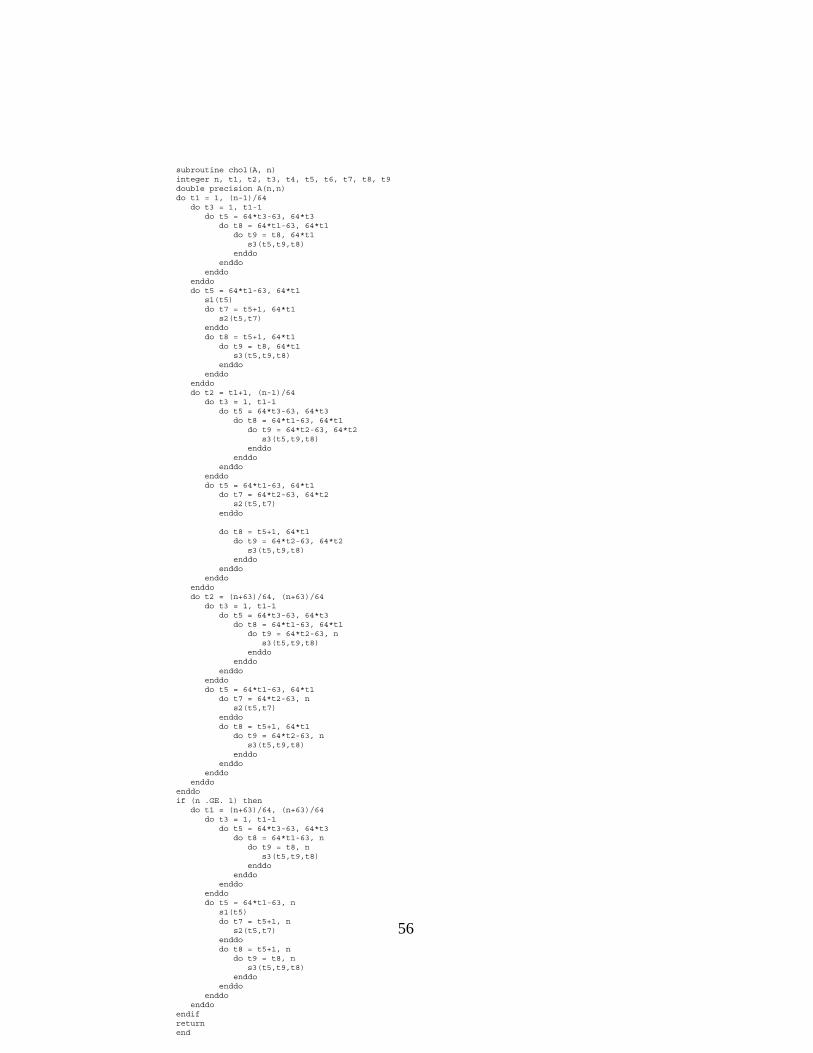
subroutine chol(A, n)integer n, t1, t2, t3, t4, t5, t6, t7, t8, t9double precision A(n,n)do t1 = 1, (n-1)/64

do t3 = 1, t1-1do t5 = 64*t3-63, 64*t3

do t8 = 64*t1-63, 64*t1do t9 = t8, 64*t1

s3(t5,t9,t8)enddo

enddoenddo

enddodo t5 = 64*t1-63, 64*t1

s1(t5)do t7 = t5+1, 64*t1

s2(t5,t7)enddodo t8 = t5+1, 64*t1

do t9 = t8, 64*t1s3(t5,t9,t8)

enddoenddo

enddodo t2 = t1+1, (n-1)/64

do t3 = 1, t1-1do t5 = 64*t3-63, 64*t3

do t8 = 64*t1-63, 64*t1do t9 = 64*t2-63, 64*t2

s3(t5,t9,t8)enddo

enddoenddo

enddodo t5 = 64*t1-63, 64*t1

do t7 = 64*t2-63, 64*t2s2(t5,t7)

enddo

do t8 = t5+1, 64*t1do t9 = 64*t2-63, 64*t2

s3(t5,t9,t8)enddo

enddoenddo

enddodo t2 = (n+63)/64, (n+63)/64

do t3 = 1, t1-1do t5 = 64*t3-63, 64*t3

do t8 = 64*t1-63, 64*t1do t9 = 64*t2-63, n

s3(t5,t9,t8)enddo

enddoenddo

enddodo t5 = 64*t1-63, 64*t1

do t7 = 64*t2-63, ns2(t5,t7)

enddodo t8 = t5+1, 64*t1

do t9 = 64*t2-63, ns3(t5,t9,t8)

enddoenddo

enddoenddo

enddoif (n .GE. 1) then

do t1 = (n+63)/64, (n+63)/64do t3 = 1, t1-1

do t5 = 64*t3-63, 64*t3do t8 = 64*t1-63, n

do t9 = t8, ns3(t5,t9,t8)

enddoenddo

enddoenddodo t5 = 64*t1-63, n

s1(t5)do t7 = t5+1, n

s2(t5,t7)enddodo t8 = t5+1, n

do t9 = t8, ns3(t5,t9,t8)

enddoenddo

enddoenddo

endifreturnend

56