data analytics for real-world business problems

DATA ANALYTICS FOR SOLVING BUSINESS PROBLEMS:

SHIFTING FOCUS FROM THE TECHNOLOGY DEPLOYMENT TO THE ANALYTICS METHODOLOGY

Alexander Kolker, PhDMarch 7, 2017

Alexander Kolker. All rights reserved 1


"Making better business decisions using data“

a co-hosted event with Accelerate Madison and Big

Data Madison Meetup

Date: February 13, 2017

Time: 5:30 PM - 7:30 PM CST

Key point:

Focusing on business outcomes rather than on data and

technology per se is getting momentum …

Some professional highlights…• 4 business consulting projects: US Bank, Boston Consulting Group,

Children’s Hospital of Wisconsin, Ohio Hospital Association

• 12 years at GE (General Electric) Healthcare: Data Scientist

• 3 years at Froedtert Hospital: Process Simulation Leader

• 5 years at Children’s Hospital of Wisconsin: Simulation and Data Analytics

• UW-Milwaukee Lubar School of Business-Adjunct Faculty: A graduate course Healthcare Delivery Systems-Data Analytics

• Lead Editor and Author of 2 books, 8 book chapters, 10 reviewed papers, 18 Conference presentation in the area of operations management, process modeling and simulation, business analytics Alexander Kolker. All rights reserved

BIG DATA AND ANALYTICS BACKGROUND


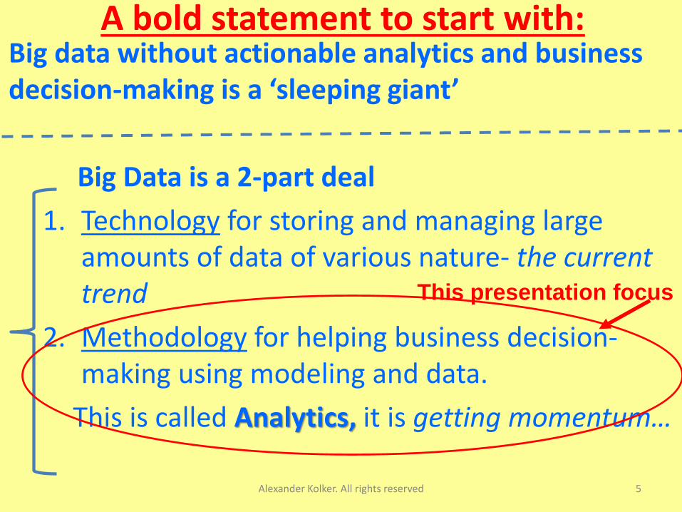
A bold statement to start with:Big data without actionable analytics and business decision-making is a ‘sleeping giant’

Big Data is a 2-part deal

1. Technology for storing and managing large amounts of data of various nature- the current trend

2. Methodology for helping business decision-making using modeling and data.

This is called Analytics, it is getting momentum…


This presentation focus

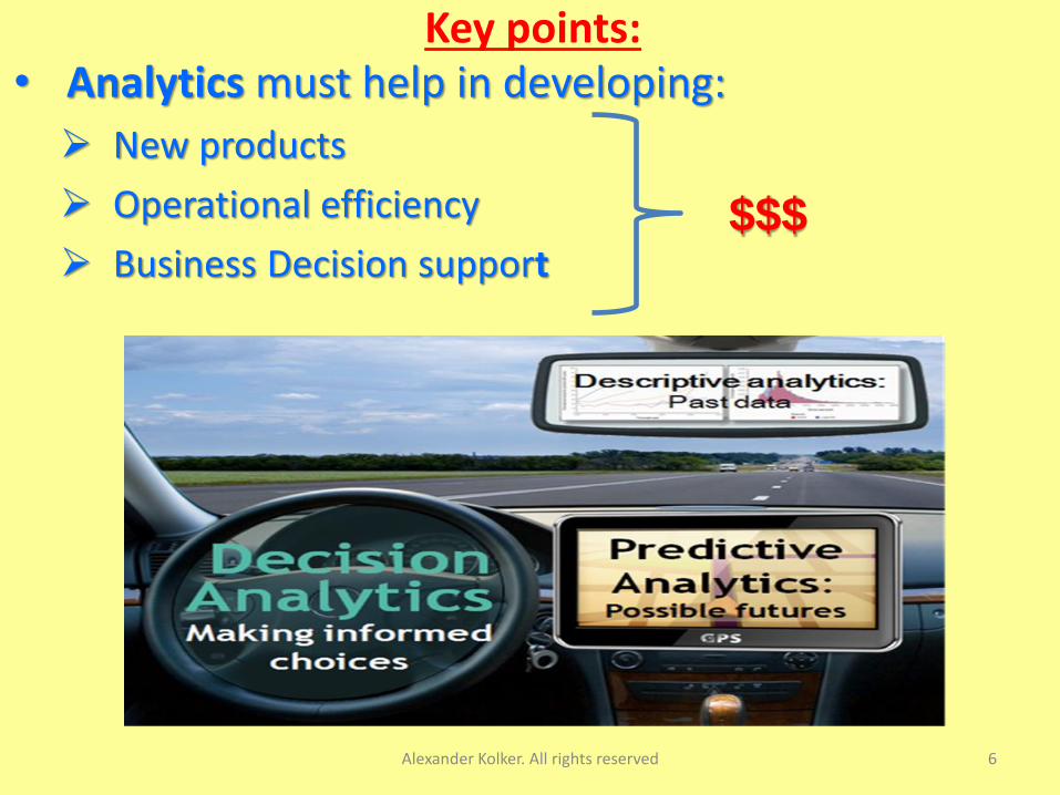
Key points:• Analytics must help in developing:

New products

Operational efficiency

Business Decision support


$$$

7

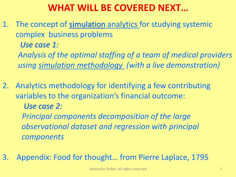
WHAT WILL BE COVERED NEXT…

1. The concept of simulation analytics for studying systemic complex business problems

Use case 1: Analysis of the optimal staffing of a team of medical providers using simulation methodology (with a live demonstration)

2. Analytics methodology for identifying a few contributing variables to the organization’s financial outcome:

Use case 2: Principal components decomposition of the large observational dataset and regression with principal components

3. Appendix: Food for thought… from Pierre Laplace, 1795Alexander Kolker. All rights reserved


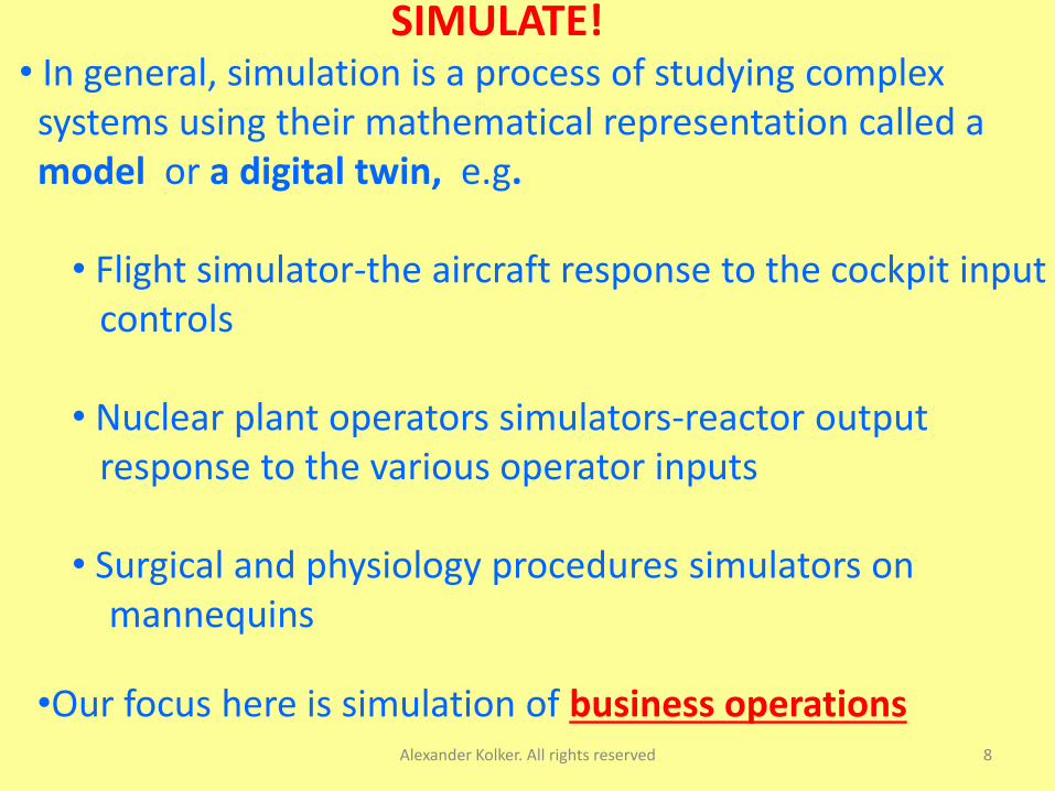
SIMULATE!• In general, simulation is a process of studying complex

systems using their mathematical representation called a model or a digital twin, e.g.

• Flight simulator-the aircraft response to the cockpit input controls

• Nuclear plant operators simulators-reactor output response to the various operator inputs

• Surgical and physiology procedures simulators on mannequins

•Our focus here is simulation of business operations


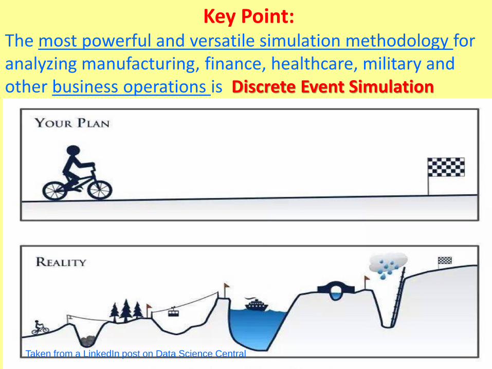
Key Point:The most powerful and versatile simulation methodology for analyzing manufacturing, finance, healthcare, military and other business operations is Discrete Event Simulation

Taken from a LinkedIn post on Data Science Central


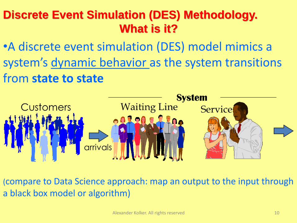
Discrete Event Simulation (DES) Methodology.

What is it?

•A discrete event simulation (DES) model mimics a system’s dynamic behavior as the system transitions from state to state

(compare to Data Science approach: map an output to the input through a black box model or algorithm)


The validated model is used for predicting various scenarios of the future system’s responses to the random inputs in a virtual reality

Key points:•The simulation model is not a ‘black box’. It is a scalable

digital twin of the reality

•The model reflects what’s actually happening in the system

• This capability gives a sense of the expected system’s output before incurring the cost and risk of thebusiness solution implementation

(compare to Data Science validation and cross-validation of a ‘black box’ model for

predicting the future outcomes…)


Use case 1

Analysis of the performance and the

optimal staffing

in an Endoscopy Unit using

Discrete Event Simulation

Presented at the:

5-th International Conference on Healthcare Systems, October, 2008;

and

IEEE Workshop on HealthCare Modeling and Simulation, February 18-20, 2010,

Venice, Italy

Problem Description

• The inevitable variability of the admission, recovery and

procedure time due to unforeseen medical complications

and delays result in some unit performance issues:

a long patient wait time to schedule procedures

not meeting daily patient demand for procedures

underutilization of the available capacity and staff

overtime

dissatisfaction of patients and medical staff

There has also been a lower than anticipated revenue

stream

The objectives of this work were:

(i) to analyze the main factors that contribute to the

inefficient patient flow and process bottlenecks,

and

(ii) to propose a more efficient patient scheduling and

staffing allocation aimed at increasing the number of

served patients, reducing procedure delays, and staff

overtime

Business Problem - Project Goal

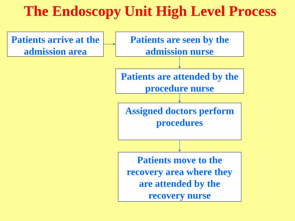
The Endoscopy Unit High Level Process

Patients arrive at the

admission area

Patients are seen by the

admission nurse

Patients are attended by the

procedure nurse

Assigned doctors perform

procedures

Patients move to the

recovery area where they

are attended by the

recovery nurse

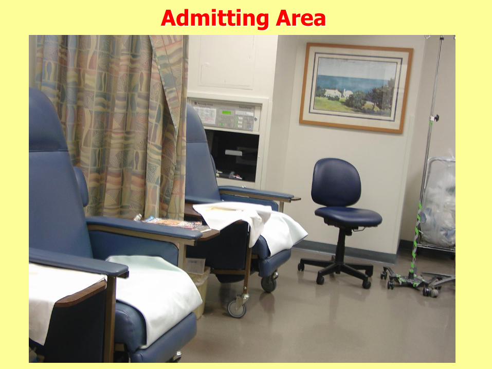
Admitting Area

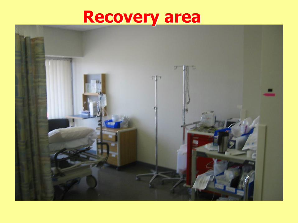
Recovery area

High Level Model Outline

• Admission, procedure and the patient recovery

duration are random variables

• These variables are represented as the best fit

statistical distributions built into the simulation model

• Each patient is assigned his/her attributes:

scheduled arrival time

procedure type

assigned doctor’s name

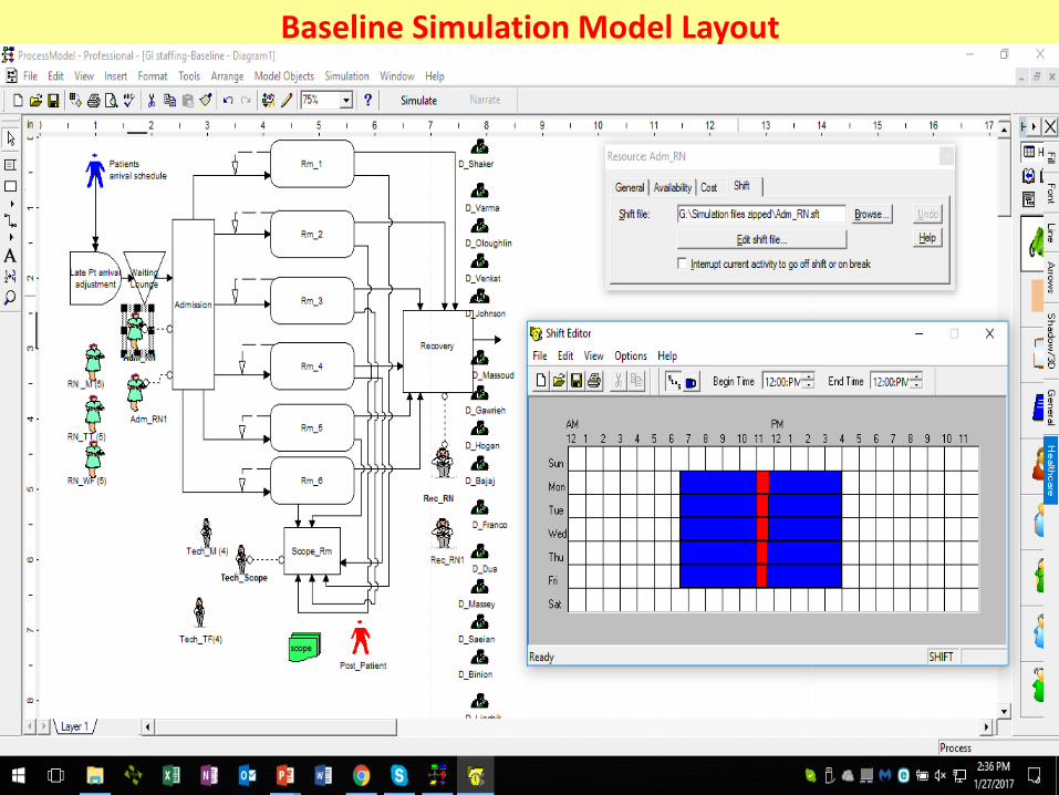
Baseline Simulation Model Layout

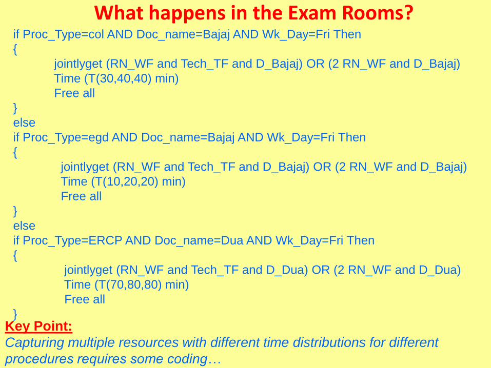
What happens in the Exam Rooms?if Proc_Type=col AND Doc_name=Bajaj AND Wk_Day=Fri Then

{

jointlyget (RN_WF and Tech_TF and D_Bajaj) OR (2 RN_WF and D_Bajaj)

Time (T(30,40,40) min)

Free all

}

else

if Proc_Type=egd AND Doc_name=Bajaj AND Wk_Day=Fri Then

{

jointlyget (RN_WF and Tech_TF and D_Bajaj) OR (2 RN_WF and D_Bajaj)

Time (T(10,20,20) min)

Free all

}

else

if Proc_Type=ERCP AND Doc_name=Dua AND Wk_Day=Fri Then

{

jointlyget (RN_WF and Tech_TF and D_Dua) OR (2 RN_WF and D_Dua)

Time (T(70,80,80) min)

Free all

}Key Point:

Capturing multiple resources with different time distributions for different

procedures requires some coding…

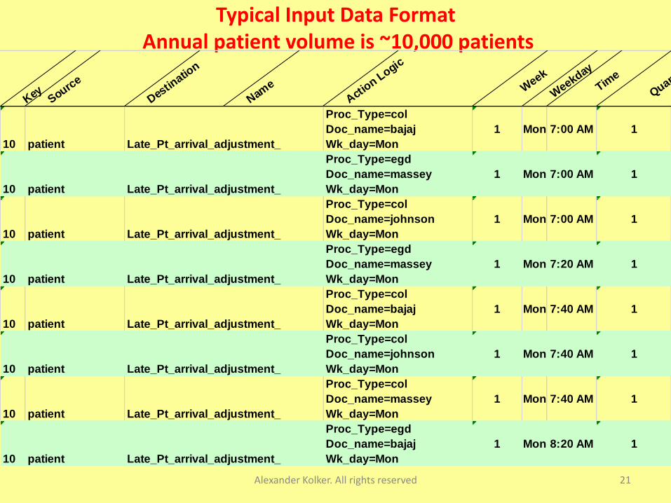
Typical Input Data FormatAnnual patient volume is ~10,000 patients


Key Source

Destin

ation

Name

Actio

n Logic

Week

Weekday

Time

Quantity

10 patient Late_Pt_arrival_adjustment_

Proc_Type=col

Doc_name=bajaj

Wk_day=Mon

1 Mon 7:00 AM 1


Proc_Type=egd

Doc_name=massey

Wk_day=Mon

1 Mon 7:00 AM 1


Proc_Type=col

Doc_name=johnson

Wk_day=Mon

1 Mon 7:00 AM 1


Proc_Type=egd

Doc_name=massey

Wk_day=Mon

1 Mon 7:20 AM 1


Proc_Type=col

Doc_name=bajaj

Wk_day=Mon

1 Mon 7:40 AM 1


Proc_Type=col

Doc_name=johnson

Wk_day=Mon

1 Mon 7:40 AM 1


Proc_Type=col

Doc_name=massey

Wk_day=Mon

1 Mon 7:40 AM 1


Proc_Type=egd

Doc_name=bajaj

Wk_day=Mon

1 Mon 8:20 AM 1


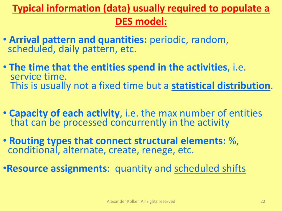
Typical information (data) usually required to populate a DES model:

• Arrival pattern and quantities: periodic, random, scheduled, daily pattern, etc.

• The time that the entities spend in the activities, i.e. service time. This is usually not a fixed time but a statistical distribution.

• Capacity of each activity, i.e. the max number of entitiesthat can be processed concurrently in the activity

• Routing types that connect structural elements: %, conditional, alternate, create, renege, etc.

•Resource assignments: quantity and scheduled shifts

Live simulation demonstration is included

here: call simulation ProcessModel

patient arrivals, shifts for nurses,

technicians and doctors, stat-fit distribution

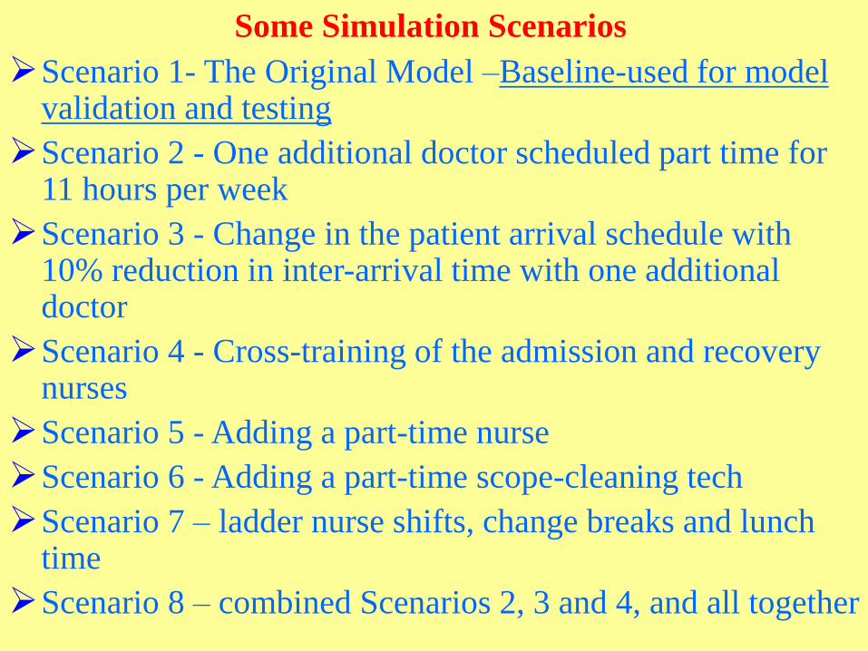
Some Simulation Scenarios

Scenario 1- The Original Model –Baseline-used for model validation and testing

Scenario 2 - One additional doctor scheduled part time for 11 hours per week

Scenario 3 - Change in the patient arrival schedule with 10% reduction in inter-arrival time with one additional doctor

Scenario 4 - Cross-training of the admission and recovery nurses

Scenario 5 - Adding a part-time nurse

Scenario 6 - Adding a part-time scope-cleaning tech

Scenario 7 – ladder nurse shifts, change breaks and lunch time

Scenario 8 – combined Scenarios 2, 3 and 4, and all together

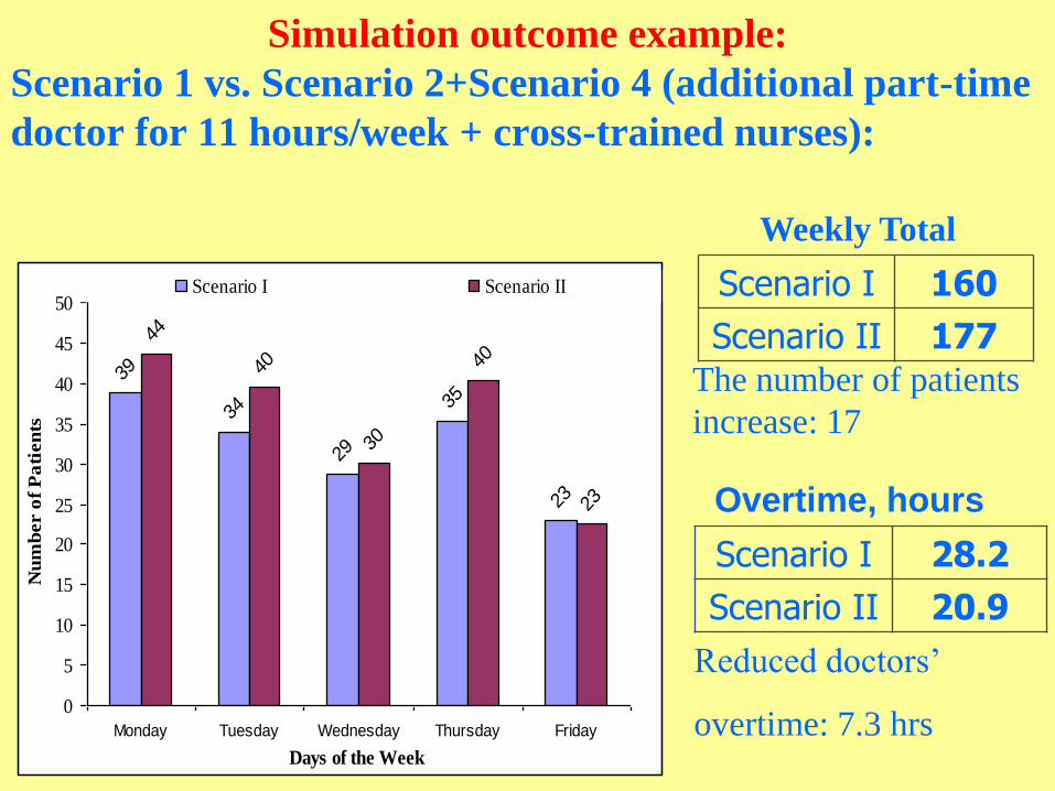
Simulation outcome example:

Scenario 1 vs. Scenario 2+Scenario 4 (additional part-time

doctor for 11 hours/week + cross-trained nurses):

39

34

29

35

23

44

40

30

40

23

0

5

10

15

20

25

30

35

40

45

50

Monday Tuesday Wednesday Thursday Friday

Days of the Week

Nu

mb

er o

f P

ati

en

ts

Scenario I Scenario II

Weekly Total

Scenario I 160

Scenario II 177The number of patients

increase: 17

Overtime, hours

Scenario I 28.2

Scenario II 20.9

Reduced doctors’

overtime: 7.3 hrs

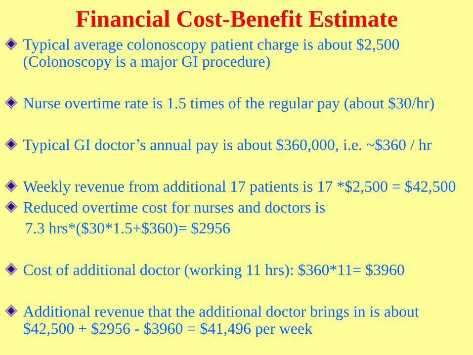
Financial Cost-Benefit EstimateTypical average colonoscopy patient charge is about $2,500 (Colonoscopy is a major GI procedure)

Nurse overtime rate is 1.5 times of the regular pay (about $30/hr)

Typical GI doctor’s annual pay is about $360,000, i.e. ~$360 / hr

Weekly revenue from additional 17 patients is 17 *$2,500 = $42,500

Reduced overtime cost for nurses and doctors is

7.3 hrs*($30*1.5+$360)= $2956

Cost of additional doctor (working 11 hrs): $360*11= $3960

Additional revenue that the additional doctor brings in is about $42,500 + $2956 - $3960 = $41,496 per week

27

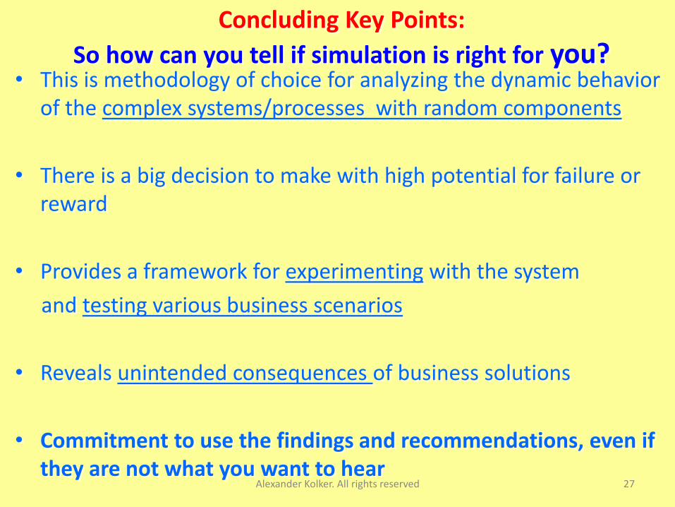
Concluding Key Points:

So how can you tell if simulation is right for you? • This is methodology of choice for analyzing the dynamic behavior

of the complex systems/processes with random components

• There is a big decision to make with high potential for failure or reward

• Provides a framework for experimenting with the system

and testing various business scenarios

• Reveals unintended consequences of business solutions

• Commitment to use the findings and recommendations, even if they are not what you want to hear

Alexander Kolker. All rights reserved

Use case 2Analytics methodology for identifying a few contributing variables to the organization’s financial outcome:Principal components decomposition of the large observational dataset and regression with Principal components

Reference: A. Kolker. Management Engineering for Effective Healthcare Delivery: Principles and Applications, IGI-Global, 2011, Chapter 1.

A. Kolker. Healthcare Management Engineering. What Does this Fancy Term Really Mean? Chapter 5. Springer-Briefs in Healthcare Management & Economics, NY, 2012


• The large local hospital plans a major market share expansion to improve its long-term financial viability


Business Problem - Project Goal

• The management wants to know what population demographic factors and population disease prevalence specific to the local area zip codes are the most important contributors to financial contribution margin (CM $)?

Note: Contribution margin is defined as the difference between all

payments collected from patients and the patient variable costs.

Plan of the problem attack


• Step 1

Demographics data matrix (total 38 variables) to be analyzed

for the top 10 ZIPs using Principal Component decomposition.

• Step 2

Regression analysis to be performed that relates $ CM and

principal components of the original data matrix.

• Step 3

By analyzing eigenvectors for only statistically significant principal

components, conclusions to be made which demographic variables

are the biggest contributors for the top 10 ZIPs


Description of Data

A set of population demographic data was collected for

local area zip codes and the corresponding median

contribution margin for each zip code (CM $).

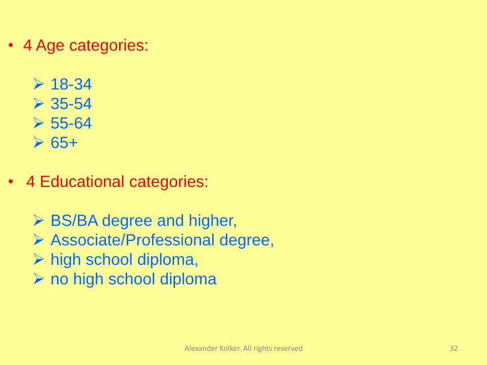
The following groups of demographic variables and

disease prevalence data were collected for each zip

code as percentage of the total zip code population:


• 4 Age categories:

18-34

35-54

55-64

65+

• 4 Educational categories:

BS/BA degree and higher,

Associate/Professional degree,

high school diploma,

no high school diploma


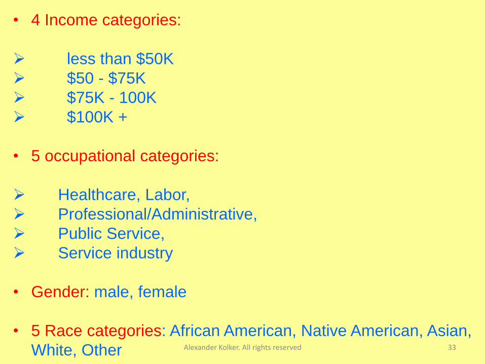
• 4 Income categories:

less than $50K

$50 - $75K

$75K - 100K

$100K +

• 5 occupational categories:

Healthcare, Labor,

Professional/Administrative,

Public Service,

Service industry

• Gender: male, female

• 5 Race categories: African American, Native American, Asian,

White, Other


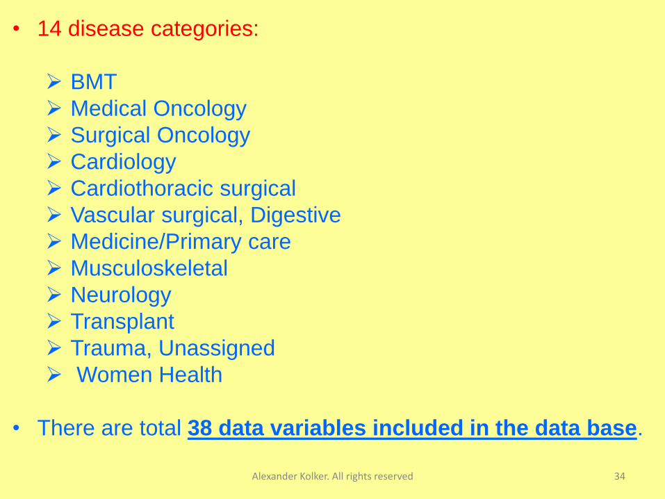
• 14 disease categories:

BMT

Medical Oncology

Surgical Oncology

Cardiology

Cardiothoracic surgical

Vascular surgical, Digestive

Medicine/Primary care

Musculoskeletal

Neurology

Transplant

Trauma, Unassigned

Women Health

• There are total 38 data variables included in the data base.


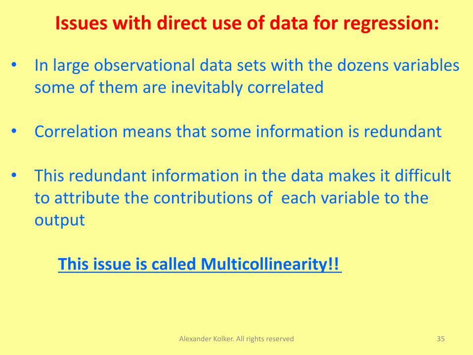
Issues with direct use of data for regression:

• In large observational data sets with the dozens variables some of them are inevitably correlated

• Correlation means that some information is redundant

• This redundant information in the data makes it difficult to attribute the contributions of each variable to the output

This issue is called Multicollinearity!!


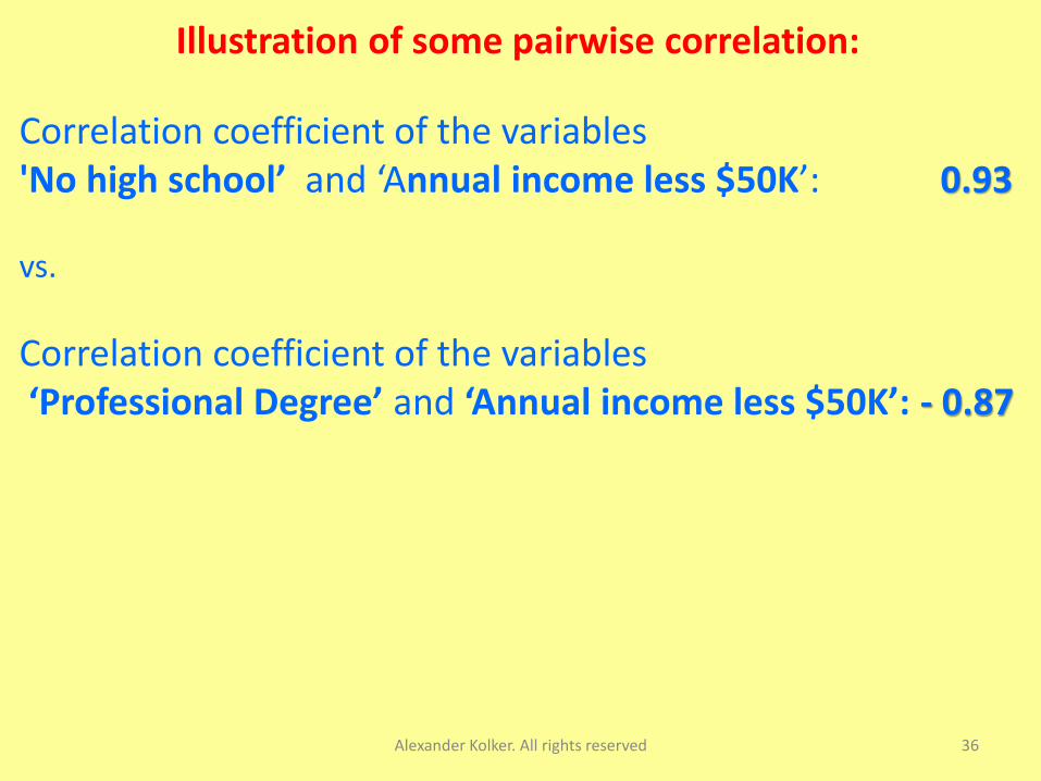
Illustration of some pairwise correlation:

Correlation coefficient of the variables 'No high school’ and ‘Annual income less $50K’: 0.93

vs.

Correlation coefficient of the variables ‘Professional Degree’ and ‘Annual income less $50K’: - 0.87


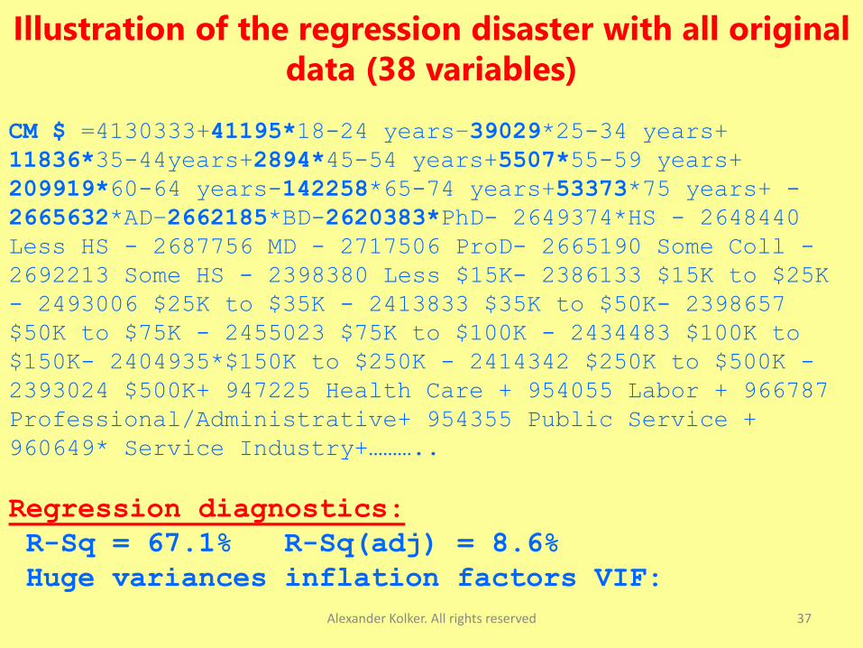
Illustration of the regression disaster with all original

data (38 variables)

CM $ =4130333+41195*18-24 years–39029*25-34 years+

11836*35-44years+2894*45-54 years+5507*55-59 years+

209919*60-64 years-142258*65-74 years+53373*75 years+ -

2665632*AD–2662185*BD-2620383*PhD- 2649374*HS - 2648440

Less HS - 2687756 MD - 2717506 ProD- 2665190 Some Coll -

2692213 Some HS - 2398380 Less $15K- 2386133 $15K to $25K

- 2493006 $25K to $35K - 2413833 $35K to $50K- 2398657

$50K to $75K - 2455023 $75K to $100K - 2434483 $100K to

$150K- 2404935*$150K to $250K - 2414342 $250K to $500K -

2393024 $500K+ 947225 Health Care + 954055 Labor + 966787

Professional/Administrative+ 954355 Public Service +

960649* Service Industry+………..

Regression diagnostics:

R-Sq = 67.1% R-Sq(adj) = 8.6%

Huge variances inflation factors VIF:


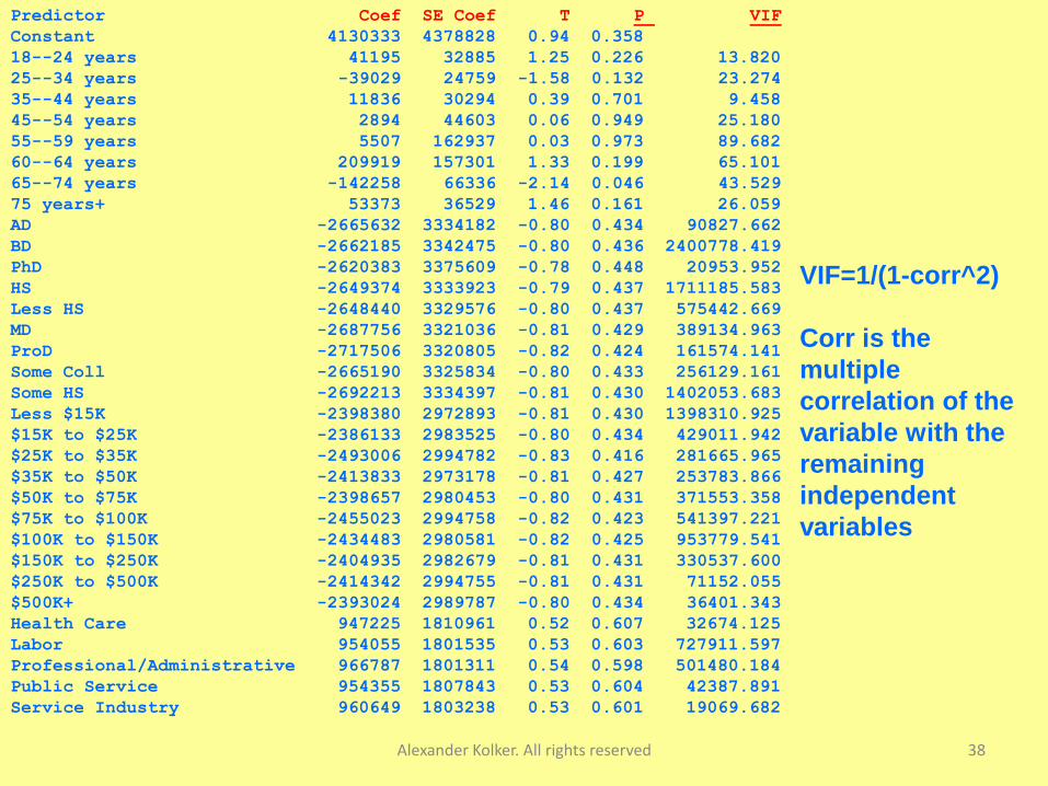
Predictor Coef SE Coef T P VIF

Constant 4130333 4378828 0.94 0.358

18--24 years 41195 32885 1.25 0.226 13.820

25--34 years -39029 24759 -1.58 0.132 23.274

35--44 years 11836 30294 0.39 0.701 9.458

45--54 years 2894 44603 0.06 0.949 25.180

55--59 years 5507 162937 0.03 0.973 89.682

60--64 years 209919 157301 1.33 0.199 65.101

65--74 years -142258 66336 -2.14 0.046 43.529

75 years+ 53373 36529 1.46 0.161 26.059

AD -2665632 3334182 -0.80 0.434 90827.662

BD -2662185 3342475 -0.80 0.436 2400778.419

PhD -2620383 3375609 -0.78 0.448 20953.952

HS -2649374 3333923 -0.79 0.437 1711185.583

Less HS -2648440 3329576 -0.80 0.437 575442.669

MD -2687756 3321036 -0.81 0.429 389134.963

ProD -2717506 3320805 -0.82 0.424 161574.141

Some Coll -2665190 3325834 -0.80 0.433 256129.161

Some HS -2692213 3334397 -0.81 0.430 1402053.683

Less $15K -2398380 2972893 -0.81 0.430 1398310.925

$15K to $25K -2386133 2983525 -0.80 0.434 429011.942

$25K to $35K -2493006 2994782 -0.83 0.416 281665.965

$35K to $50K -2413833 2973178 -0.81 0.427 253783.866

$50K to $75K -2398657 2980453 -0.80 0.431 371553.358

$75K to $100K -2455023 2994758 -0.82 0.423 541397.221

$100K to $150K -2434483 2980581 -0.82 0.425 953779.541

$150K to $250K -2404935 2982679 -0.81 0.431 330537.600

$250K to $500K -2414342 2994755 -0.81 0.431 71152.055

$500K+ -2393024 2989787 -0.80 0.434 36401.343

Health Care 947225 1810961 0.52 0.607 32674.125

Labor 954055 1801535 0.53 0.603 727911.597

Professional/Administrative 966787 1801311 0.54 0.598 501480.184

Public Service 954355 1807843 0.53 0.604 42387.891

Service Industry 960649 1803238 0.53 0.601 19069.682

VIF=1/(1-corr^2)

Corr is the

multiple

correlation of the

variable with the

remaining

independent

variables


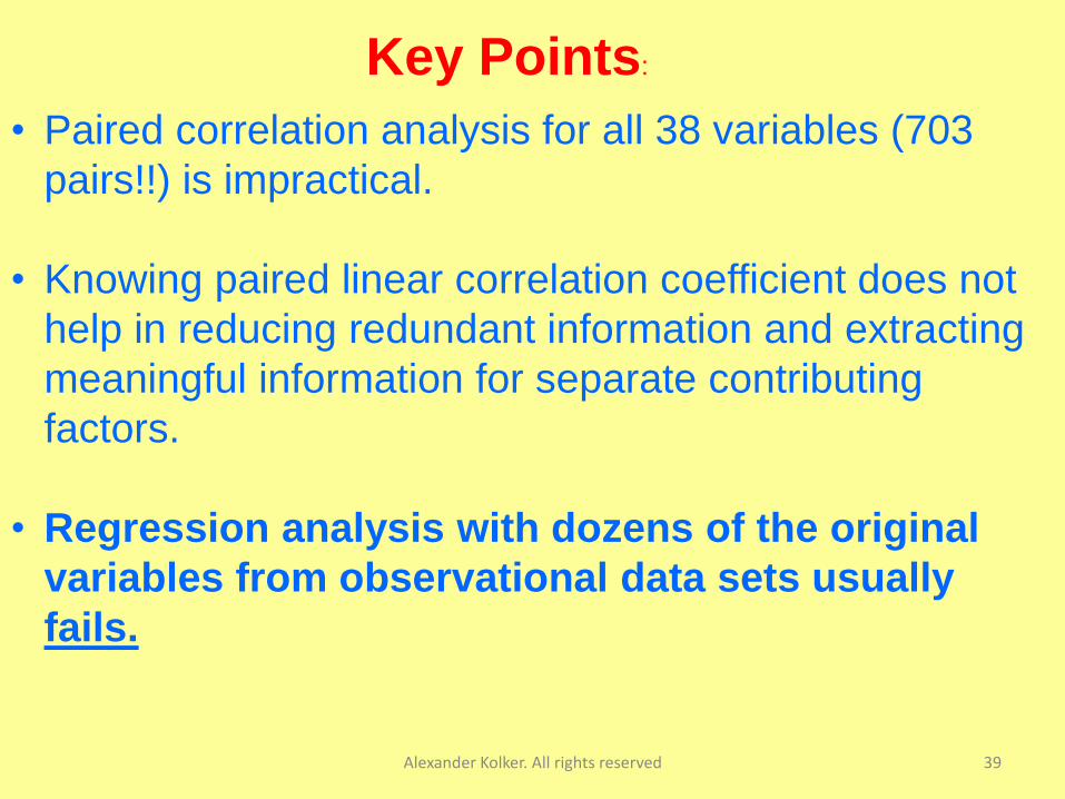
• Paired correlation analysis for all 38 variables (703

pairs!!) is impractical.

• Knowing paired linear correlation coefficient does not

help in reducing redundant information and extracting

meaningful information for separate contributing

factors.

• Regression analysis with dozens of the original

variables from observational data sets usually

fails.

Key Points:


• It allows removing the redundant

variables that carry little or no information

while retaining only a few mutually

uncorrelated principal variables.

Why Principal components

decomposition?

The main idea of PCD


The purpose of PCD is determining r new variables

PCr that can best approximate variation in the p

original X variables as linear combinations

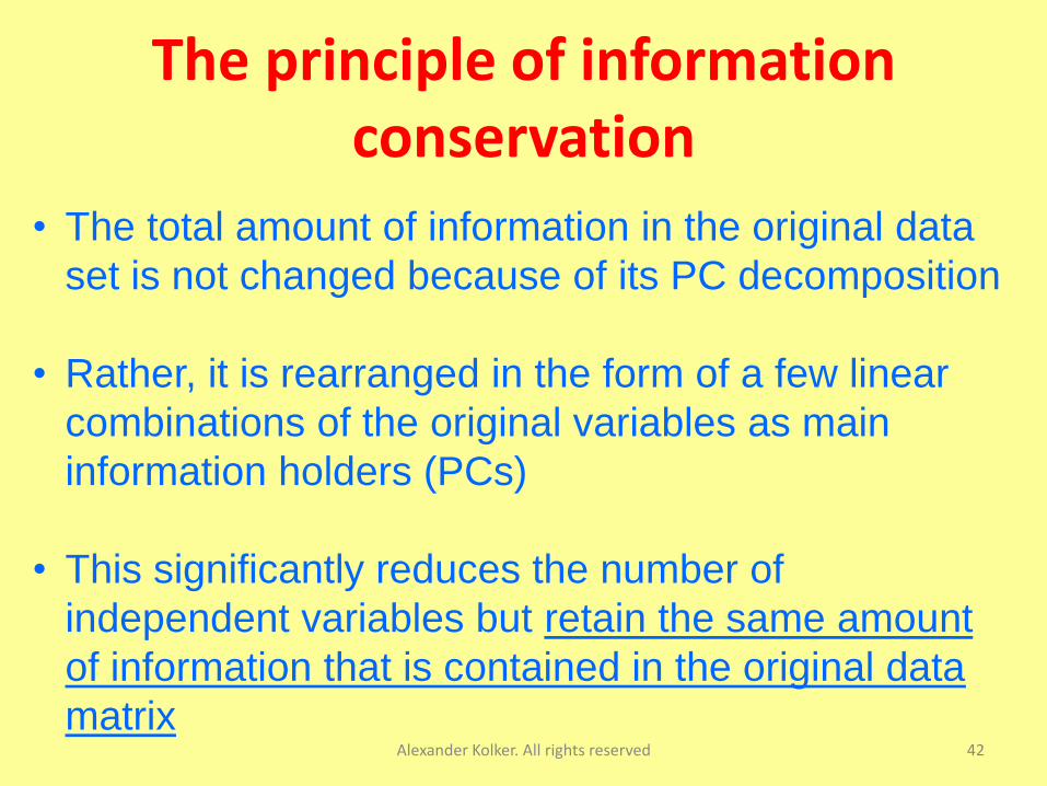
The principle of information conservation


• The total amount of information in the original data

set is not changed because of its PC decomposition

• Rather, it is rearranged in the form of a few linear

combinations of the original variables as main

information holders (PCs)

• This significantly reduces the number of

independent variables but retain the same amount

of information that is contained in the original data

matrix

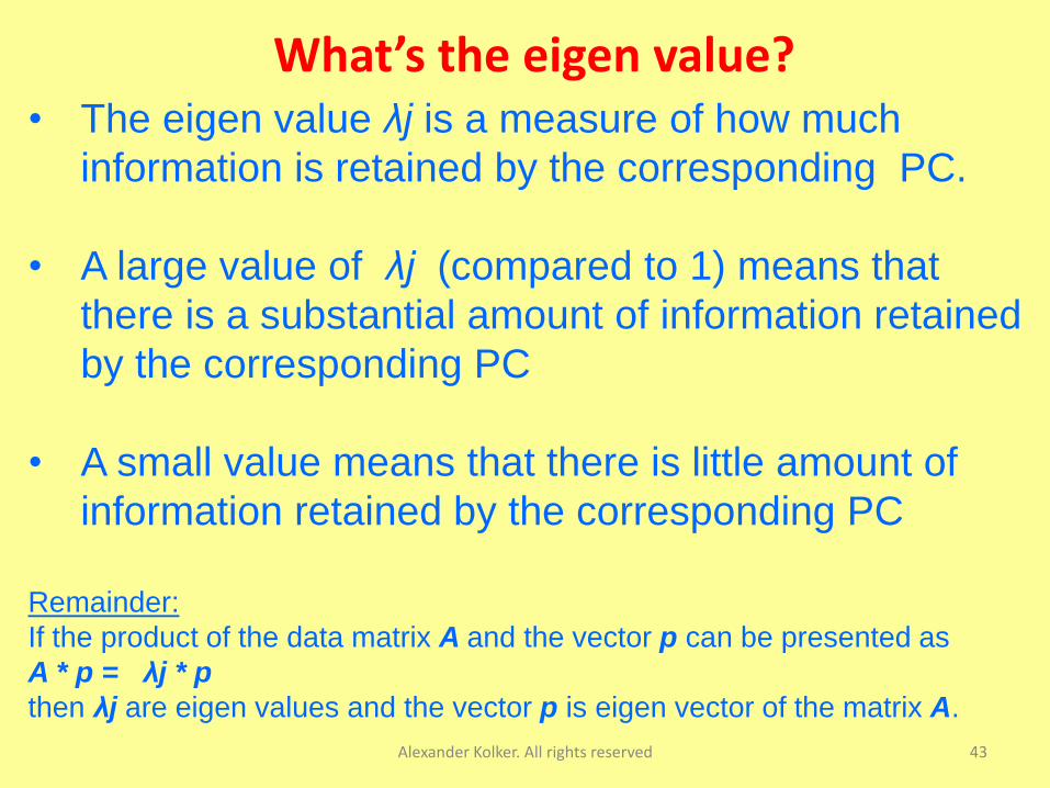
What’s the eigen value?


• The eigen value λj is a measure of how much

information is retained by the corresponding PC.

• A large value of λj (compared to 1) means that

there is a substantial amount of information retained

by the corresponding PC

• A small value means that there is little amount of

information retained by the corresponding PC

Remainder:

If the product of the data matrix A and the vector p can be presented as

A * p = λj * p

then λj are eigen values and the vector p is eigen vector of the matrix A.

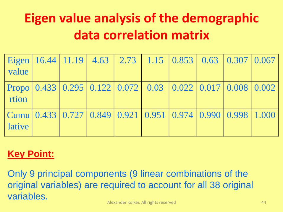
Eigen value analysis of the demographic data correlation matrix


Eigen

value

16.44 11.19 4.63 2.73 1.15 0.853 0.63 0.307 0.067

Propo

rtion

0.433 0.295 0.122 0.072 0.03 0.022 0.017 0.008 0.002

Cumu

lative

0.433 0.727 0.849 0.921 0.951 0.974 0.990 0.998 1.000

Key Point:

Only 9 principal components (9 linear combinations of the

original variables) are required to account for all 38 original

variables.


Why Regression with Principal components?

• Because PCs are mutually uncorrelated, the

variation of dependent variable (CM $) is accounted

for by each PC independently of other PC

• Contribution of each PC is directly defined by the

coefficients of the regression equation

Key Point:

Regression with totally uncorrelated PC is one of the

most powerful methodologies for identifying significant

contributing variables (factors).

The Best Subset Regression


• Best subsets regression identifies the best-fitting

regression models that can be constructed with as

few predictor variables as possible

• All possible subsets of the predictors are examined,

beginning with all models containing one predictor,

and then all models containing two predictors, and so

on.

• The two best models for each number of predictors

are displayed

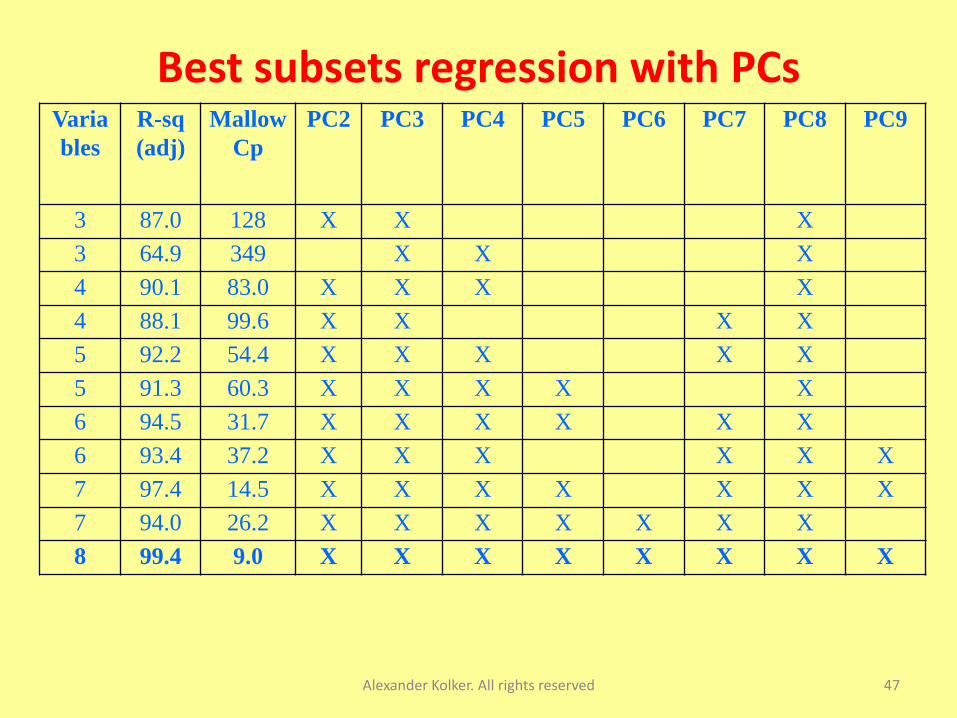
Best subsets regression with PCs


Varia

bles

R-sq

(adj)

Mallow

Cp

PC2 PC3 PC4 PC5 PC6 PC7 PC8 PC9

3 87.0 128 X X X

3 64.9 349 X X X

4 90.1 83.0 X X X X

4 88.1 99.6 X X X X

5 92.2 54.4 X X X X X

5 91.3 60.3 X X X X X

6 94.5 31.7 X X X X X X

6 93.4 37.2 X X X X X X

7 97.4 14.5 X X X X X X X

7 94.0 26.2 X X X X X X X

8 99.4 9.0 X X X X X X X X

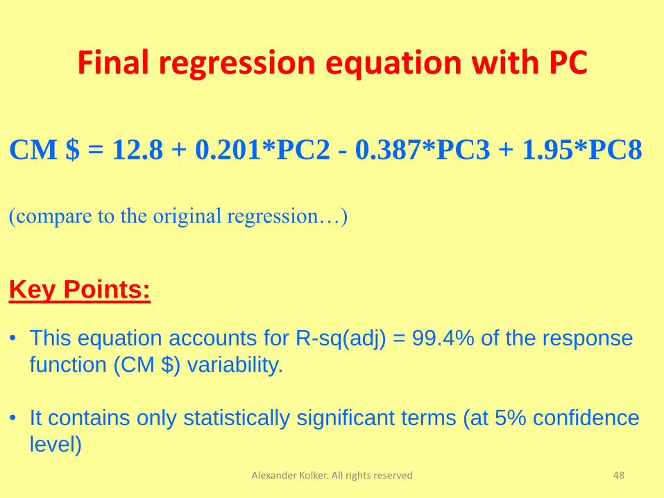
Final regression equation with PC


CM $ = 12.8 + 0.201*PC2 - 0.387*PC3 + 1.95*PC8

(compare to the original regression…)

Key Points:

• This equation accounts for R-sq(adj) = 99.4% of the response

function (CM $) variability.

• It contains only statistically significant terms (at 5% confidence

level)

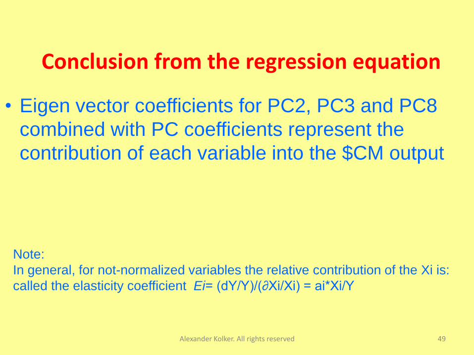
Conclusion from the regression equation


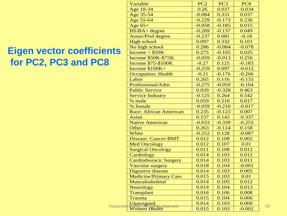
• Eigen vector coefficients for PC2, PC3 and PC8

combined with PC coefficients represent the

contribution of each variable into the $CM output

Note:

In general, for not-normalized variables the relative contribution of the Xi is:

called the elasticity coefficient Ei= (dY/Y)/(∂Xi/Xi) = ai*Xi/Y


Variable PC2 PC3 PC8

Age 18-34 0.26 0.037 -0.034

Age 35-54 -0.084 0.331 0.037

Age 55-64 -0.229 -0.173 0.236

Age 65+ -0.058 -0.185 0.015

BS/BA+ degree -0.269 -0.137 0.049

Assoc/Prof degree -0.237 0.081 -0.18

High school 0.097 0.332 0.101

No high school 0.286 -0.084 -0.078

Income < $50K 0.275 -0.105 0.025

Income $50K-$75K -0.059 -0.013 0.256

Income $75-$100K -0.27 0.125 -0.183

Income $100K+ -0.259 0.097 -0.012

Occupation: Health -0.21 -0.176 -0.206

Labor 0.265 0.116 -0.133

Professional/Adm -0.275 -0.059 -0.104

Public Service 0.029 -0.328 0.463

Service Industry -0.125 0.264 0.542

% male 0.059 0.210 0.017

% female -0.059 -0.210 -0.017

Race: African American 0.235 -0.123 0.007

Asian 0.157 0.142 -0.337

Native American -0.033 -0.339 -0.253

Other 0.263 -0.114 0.158

White -0.252 0.128 -0.087

Disease: Cancer-BMT 0.012 0.108 0.002

Med Oncology 0.012 0.107 0.01

Surgical Oncology 0.011 0.108 0.012

Cardiology 0.014 0.103 0.012

Cardiothoracic Surgery 0.014 0.103 0.011

Vascular surgery 0.018 0.104 -0.001

Digestive disease 0.014 0.103 0.005

Medicine/Primary Care 0.015 0.103 0.01

Musculoskeletal 0.014 0.105 0.012

Neurology 0.014 0.104 0.013

Transplant 0.016 0.106 0.008

Trauma 0.015 0.104 0.006

Unassigned 0.014 0.103 0.000

Women Health 0.015 0.103 -0.002

Eigen vector coefficients

for PC2, PC3 and PC8

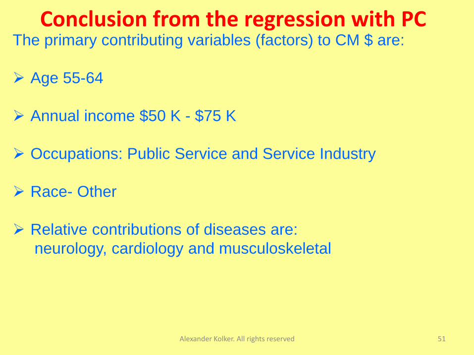
Conclusion from the regression with PC


The primary contributing variables (factors) to CM $ are:

Age 55-64

Annual income $50 K - $75 K

Occupations: Public Service and Service Industry

Race- Other

Relative contributions of diseases are:

neurology, cardiology and musculoskeletal

Concluding Remarks and Reflections


• As analytics professionals we are rewarded for help in solving

business problems

• Building analytics that influences business decision-making

requires attention to the non-technical side of the project

(organization’s internal politics and power-sharing)

• Analytics has no practical value for the organization if it does

not affect business decision-making, regardless of how much

a new trendy technology is used

So, how much of your work is about understanding and

addressing real business problems vs. the technology

deployment, coding and finding insights in the data?

Alexander Kolker. All rights reserved53

.

Appendix“We may regard the present state of the universe as the effect of its past

and the cause of its future (Predictive analytics?!)

An intellect which at a certain moment would know all forces that set

nature in motion, and all positions of all items of which nature is

composed, if this intellect were also vast enough to submit these data to

analysis, it would embrace in a single formula (algorithm?) the

movements of the greatest bodies of the universe and those of the

tiniest atom.

For such an intellect nothing would be uncertain and the future

(predictive analytics?) just like the past would be present before its

eyes.”

- Pierre Simon Laplace, A Philosophical Essay on Probabilities, 1795

Food for Thought:

Can the contemporary Big Data Technology function as that ‘intellect’

capable of analyzing all data and getting a single formula for the future?

data analytics for real-world business problems

Data & Analytics