dark energy two decades after: observables, probes ... energy two decades after: observables,...
TRANSCRIPT

Dark energy two decades after: Observables,probes, consistency tests
Dragan Huterer1 and Daniel L Shafer2
1 Department of Physics, University of Michigan, 450 Church Street, AnnArbor, MI 48109, USA
E-mail: [email protected] Department of Physics and Astronomy, Johns Hopkins University, 3400 NorthCharles Street, Baltimore, MD 21218, USA
E-mail: [email protected]
Abstract. The discovery of the accelerating universe in the late 1990s wasa watershed moment in modern cosmology, as it indicated the presence of afundamentally new, dominant contribution to the energy budget of the universe.Evidence for dark energy, the new component that causes the acceleration, hassince become extremely strong, owing to an impressive variety of increasinglyprecise measurements of the expansion history and the growth of structure in theuniverse. Still, one of the central challenges of modern cosmology is to shed lighton the physical mechanism behind the accelerating universe. In this review, webriefly summarize the developments that led to the discovery of dark energy. Next,we discuss the parametric descriptions of dark energy and the cosmological teststhat allow us to better understand its nature. We then review the cosmologicalprobes of dark energy. For each probe, we briefly discuss the physics behind itand its prospects for measuring dark energy properties. We end with a summaryof the current status of dark energy research.
Keywords: dark energy, observational cosmology, large-scale structure
PACS numbers: 98.80.Es, 95.36.+x
Submitted to: Rep. Prog. Phys.
arX
iv:1
709.
0109
1v2
[as
tro-
ph.C
O]
5 F
eb 2
018
Dark energy two decades after 2
1. Introduction
The discovery of the accelerating universe in the late1990s [1, 2] was a watershed moment in moderncosmology. It unambiguously indicated the presenceof a qualitatively new component in the universe,one that dominates the energy density today, orof a modification of the laws of gravity. Darkenergy quickly became a centerpiece of the newstandard cosmological model, which also featuresbaryonic matter, dark matter, and radiation (photonsand relativistic neutrinos). Dark energy naturallyresolved some tensions in cosmological parametermeasurements of the 1980s and early 1990s, explainingin particular the fact that the geometry of the universewas consistent with the flatness predicted by inflation,while the matter density was apparently much less thanthe critical value necessary to close the universe.
The simplest and best-known candidate for darkenergy is the energy of the vacuum, representedin Einstein’s equations by the cosmological-constantterm. Vacuum energy density, unchanging in timeand spatially smooth, is currently in good agreementwith existing data. Yet, there exists a rich set ofother dark energy models, including evolving scalarfields, modifications to general relativity, and otherphysically-motivated possibilities. This has spawnedan active research area focused on describing andmodeling dark energy and its effects on the expansionrate and the growth of density fluctuations, and thisremains a vibrant area of cosmology today.
Over the past two decades, cosmologists have beeninvestigating how best to measure the properties ofdark energy. They have studied exactly what eachcosmological probe can say about this new component,devised novel cosmological tests for the purpose, andplanned observational surveys with the principal goalof precision dark energy measurements. Both ground-based and space-based surveys have been planned, andthere are even ideas for laboratory tests of the physicalphenomena that play a role in some dark energymodels. Current measurements have already sharplyimproved constraints on dark energy; as a simpleexample, the statistical evidence for its existence,assuming a cosmological constant but not a flatuniverse, is nominally over 66σ‡. Future observations
‡ To obtain this number, we maximized the likelihood over allparameters, first with the dark energy density a free parameterand then with it fixed to zero, using the same current data as
are expected to do much better still, especially formodels that allow a time-evolving dark energy equationof state. They will allow us to map the expansionand growth history of the universe at the percent level,beginning deep in the matter-dominated era, into theperiod when dark energy dominates, and up to thepresent day.
Despite the tremendous observational progress inmeasuring dark energy properties, no fundamentallynew insights into the physics behind this mysteriouscomponent have resulted. Remarkably, while the errorbars have shrunk dramatically, current constraintsare still roughly consistent with the specific modelthat was originally quoted as the best fit in the late1990s — a component contributing about 70% tothe current energy budget with an equation-of-stateratio w ' −1. This has led some in the particlephysics and cosmology community to suspect that darkenergy really is just the cosmological constant Λ andthat its unnaturally-small value is the product of amultiverse, such as would arise from the frameworkof eternal inflation or from the landscape picture ofstring theory, which generically features an enormousnumber of vacua, each with a different value for Λ.In this picture, we live in a vacuum which is able tosupport stars, galaxies, and life, making our tiny Λa necessity rather than an accident or a signature ofnew physics. As such reasoning may be untestable andtherefore arguably unscientific, many remain hopefulthat cosmic acceleration can be explained by testablephysical theory that does not invoke the anthropicprinciple. For now, improved measurements provideby far the best opportunity to better understand thephysics behind the accelerating universe.
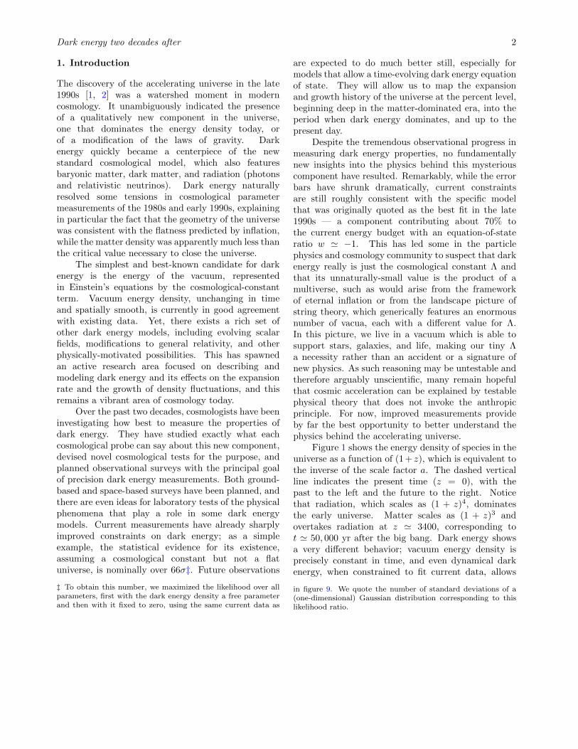
Figure 1 shows the energy density of species in theuniverse as a function of (1 + z), which is equivalent tothe inverse of the scale factor a. The dashed verticalline indicates the present time (z = 0), with thepast to the left and the future to the right. Noticethat radiation, which scales as (1 + z)4, dominatesthe early universe. Matter scales as (1 + z)3 andovertakes radiation at z ' 3400, corresponding tot ' 50, 000 yr after the big bang. Dark energy showsa very different behavior; vacuum energy density isprecisely constant in time, and even dynamical darkenergy, when constrained to fit current data, allows
in figure 9. We quote the number of standard deviations of a(one-dimensional) Gaussian distribution corresponding to thislikelihood ratio.
Dark energy two decades after 3
Figure 1. Energy density of species in the universe as a function of (1 + z), where z is the redshift. The dashed vertical lineindicates the present time (z = 0), with the past to the left and future to the right. Note that matter (∝ (1 + z)3) and radiation(∝ (1 + z)4) energy densities scale much faster with the expanding universe than the dark energy density, which is exactly constantfor a cosmological constant Λ. The shaded region for dark energy indicates the energy densities allowed at 1σ (68.3% confidence)by combined constraints from current data assuming the equation of state is allowed to vary as w(z) = w0 + wa z/(1 + z).
only a modest variation in density with time. Theshaded region in figure 1 indicates the region allowedat 1σ (68.3% confidence) by combined constraints fromcurrent data (see figure 9) assuming the equation ofstate is allowed to vary as w(a) = w0 + wa (1− a).
Our goal is to broadly review cosmic accelerationfor physicists and astronomers who have a basicfamiliarity with cosmology but may not be experts inthe field. This review complements other excellent,and often more specialized, reviews of the subject thatfocus on dark energy theory [5–7], cosmology [8], thephysics of cosmic acceleration [9], probes of dark energy[10, 11], dark energy reconstruction [12], dynamics ofdark energy models [13], the cosmological constant[14, 15], and dark energy aimed at astronomers [16].A parallel review of dark energy theory is presented inthis volume by P. Brax.
The rest of this review is organized as follows.In section 2, we provide a brief history of thediscovery of dark energy and how it changed ourunderstanding of the universe. In section 3, weoutline the mathematical formalism that underpinsmodern cosmology. In section 4, we review empiricalparametrizations of dark energy and other ways toquantify our constraints on geometry and growth ofstructure, as well as modified gravity descriptions.We review the principal cosmological probes of dark
energy in section 5 and discuss complementary probesin section 6. In section 7, we summarize key pointsregarding the observational progress on dark energy.
2. The road to dark energy
In the early 1980s, inflationary theory shook theworld of cosmology by explaining several long-standingconundrums [17–19]. The principal inflationary featureis a mechanism to accelerate the expansion rate so thatthe universe appears precisely flat at late times. As oneof inflation’s cornerstone predictions, flatness becamethe favored possibility among cosmologists. At thesame time, various direct measurements of mass in theuniverse were typically producing answers that were farshort of the amount necessary to close the universe.
Notably, the baryon-to-matter ratio measured ingalaxy clusters, combined with the baryon density in-ferred from big bang nucleosynthesis, effectively ruledout the flat, matter-dominated universe, implying in-stead a low matter density Ωm ∼ 0.3 [20–22]. Aroundthe same time, measurements of galaxy clustering —both the amplitude and shape of the correlation func-tion — indicated strong preference for a low-matter-density universe and further pointed to the concor-dance cosmology with the cosmological constant con-tributing to make the spatial geometry flat [23, 24].
Dark energy two decades after 41993ApJ...413L.105P
-20 0 20 40 60-15
-16
-17
-18
-19
-20
-20 0 20 40 60-15
-16
-17
-18
-19
-20
B Band
as measured
light-curve timescale“stretch-factor” corrected
days
MB
– 5
log(
h/65
)
days
MB
– 5
log(
h/65
)
Calan/Tololo SNe Ia
Kim, et al. (1997)
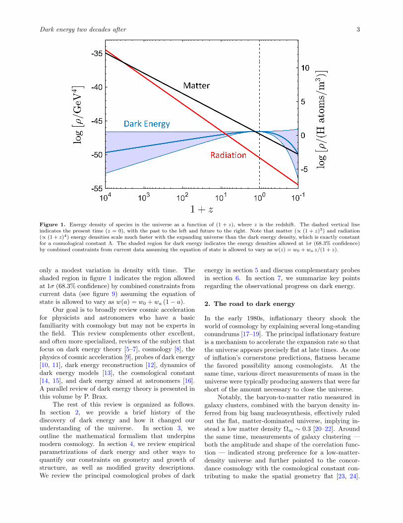
Figure 2. Key properties of type Ia supernovae that enabled them to become a powerful tool to discover the acceleration of theuniverse. Left panel : The Phillips relation, reproduced from his 1993 paper [3]. The (apparent) magnitude of SNe Ia is correlatedwith ∆m15, the decay of the light curve 15 days after the maximum. Right panel : Light curves for a sample of SNe Ia before (top)and after (bottom) correction for stretch (essentially, the Phillips relation); reproduced from [4].
The relatively high values of the measured Hubble con-stant at the time (H0 ' 80 km/s/Mpc [25]), combinedwith the lower limit on the age of the universe inferredfrom the ages of globular clusters (t0 > 11.2 Gyr at95% confidence [26]), also disfavored a high-matter-density universe. Finally, the discovery of massive clus-ters of galaxies at high redshift z ∼ 1 [27, 28] indepen-dently created trouble for the flat, matter-dominateduniverse.
While generally in agreement with measurements,such a low-density universe still conflicted with theages of globular clusters, even setting aside inflationaryprejudice for a flat universe. Also, the results were notunambiguous: throughout the 1980s and early 1990s,there was claimed evidence for a much higher matterdensity from measurements of galaxy fluxes [31] andpeculiar velocities (e.g. [32–34]), along with theoreticalforays that have since been disfavored, such as inflationmodels that result in an open universe [35, 36] andextremely low values of the Hubble constant [37]. Eventhe early type Ia supernova studies yielded inconclusiveresults [38].
Attempts to square the theoretical preference for
a flat universe with uncertain measurements of thematter density included a proposal for the existenceof a nonzero cosmological constant Λ. This term,corresponding to the energy density of the vacuum,would need to have a tiny value by particle physicsstandards in order to be comparable to the energydensity of matter today. Once considered by Einsteinto be the mechanism that guarantees a static universe[39], it was soon disfavored when it became clearthat such a static universe is unstable to smallperturbations, and it was abandoned once it becameestablished that the universe is actually expanding.Entertained as a possibility in 1980s [40, 41], thecosmological constant was back in full force in the1990s [24, 42–48]. Nevertheless, it was far fromclear that anything other than matter, plus a smallamount of radiation, comprises the energy density inthe universe today.
A breakthrough came in late 1990s. Two teamsof supernova observers, the Supernova CosmologyProject (led by Saul Perlmutter) and the High-Z Supernova Search Team (led by Brian Schmidt)developed an efficient approach to use the world’s
Dark energy two decades after 5
0 0.5 1Redshift z
-0.5
0
0.5
1
∆ (m
-M)
SNBAO
always accelerates
accelerates nowdecelerated in the past
always decelerates
flatopen
closed
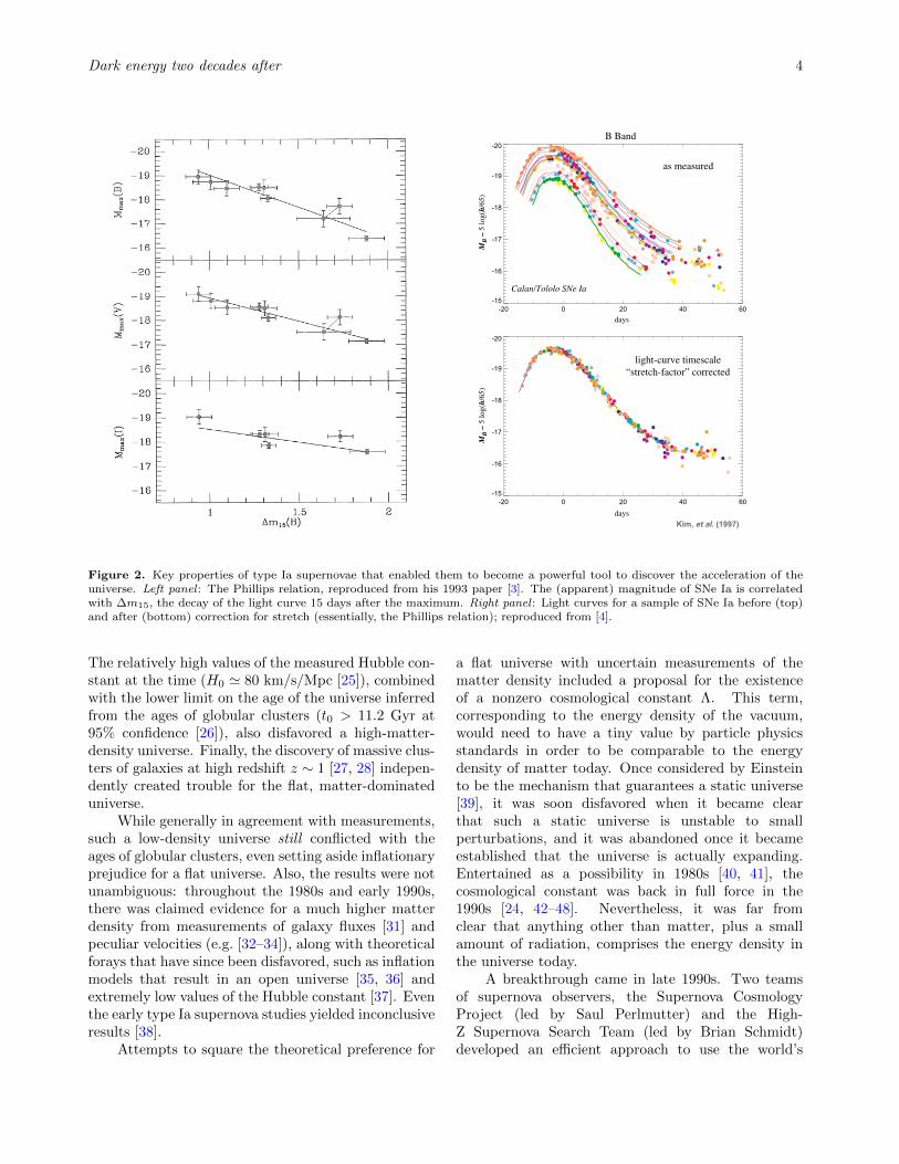
Figure 3. Evidence for the transition from deceleration in the past to acceleration today. The blue line indicates a model thatfits the data well; it features acceleration at relatively late epochs in the history of the universe, beginning a few billion years agobut still billions of years after the big bang. For comparison, we also show a range of matter-only models in green, correspondingto 0.3 ≤ Ωm ≤ 1.5 and thus spanning the open, flat, and closed geometries without dark energy. Finally, the red curve indicates amodel that always exhibits acceleration and that also does not fit the data. The black data points are binned distance moduli fromthe Supercal compilation [29] of 870 SNe, while the three red data points represent the distances inferred from the most recent BAOmeasurements (BOSS DR12 [30]).
most powerful telescopes working in concert to discoverand follow up supernovae. These teams identifiedprocedures to guarantee finding batches of SNe in eachrun (for a popular review of this, see [49]).
Another breakthrough came in 1993 by MarkPhillips, an astronomer working in Chile [3]. Henoticed that the SN Ia luminosity (or absolutemagnitude) is correlated with the decay time of theSN light curve. Phillips considered the quantity ∆m15,the decay of the light from the SN 15 days after themaximum. He found that ∆m15 is strongly correlatedwith the SN intrinsic brightness (estimated using othermethods). The Phillips relation (left panel of figure 2)is roughly the statement that “broader is brighter.”That is, SNe with broader light curves tend to havea larger intrinsic luminosity. This broadness can bequantified by a “stretch factor” that scales the widthof the light curve [2]. By applying a correction based onstretch (right panel of figure 2), astronomers found thatthe intrinsic dispersion of the SN Ia luminosity, initially∼0.3–0.5 mag, can be reduced to ∼0.2 mag aftercorrection for stretch. Note that this corresponds toan error in distance of δdL/dL = [ln(10)/5] δm ∼ 10%.The Phillips relation was the second key ingredientthat enabled SNe Ia to achieve the precision neededto reliably probe the contents of the universe.
A third important ingredient was the ability
to separate intrinsic variation in individual SNluminosities from extinction due to intervening dustalong the line of sight, which leads to reddening.This separation requires SN Ia color measurements,achieved by observing and fitting SN Ia light curvesin multiple wavebands (e.g. [50]).
The final, though chronologically the first, keystep for the discovery of dark energy was thedevelopment and application of charge-coupled devices(CCDs) in observational astronomy, and they equippedcameras of increasingly large size [51–57].
Some of the early SN Ia results came in the period1995–1997 but were based on only a few high-redshiftSNe and therefore had large uncertainties (e.g. [38]).
2.1. The discovery of dark energy
The definitive results, based on 16 [1] and 42 [2] high-redshift supernovae, followed soon thereafter. Theresults of the two teams agreed and indicated thatthe distant SNe are dimmer than would be expectedin a matter-only universe. In other words, theywere farther away than expected, suggesting that theexpansion rate of the universe is increasing, contrary tothe expectation for a matter-dominated universe withany amount of matter. Over the following decade,larger and better SN samples [58–62] confirmed andstrengthened the original findings, while discoveries of
Dark energy two decades after 6
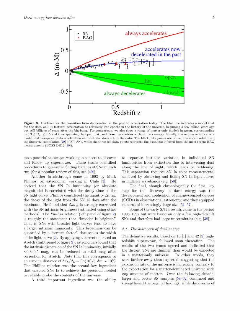
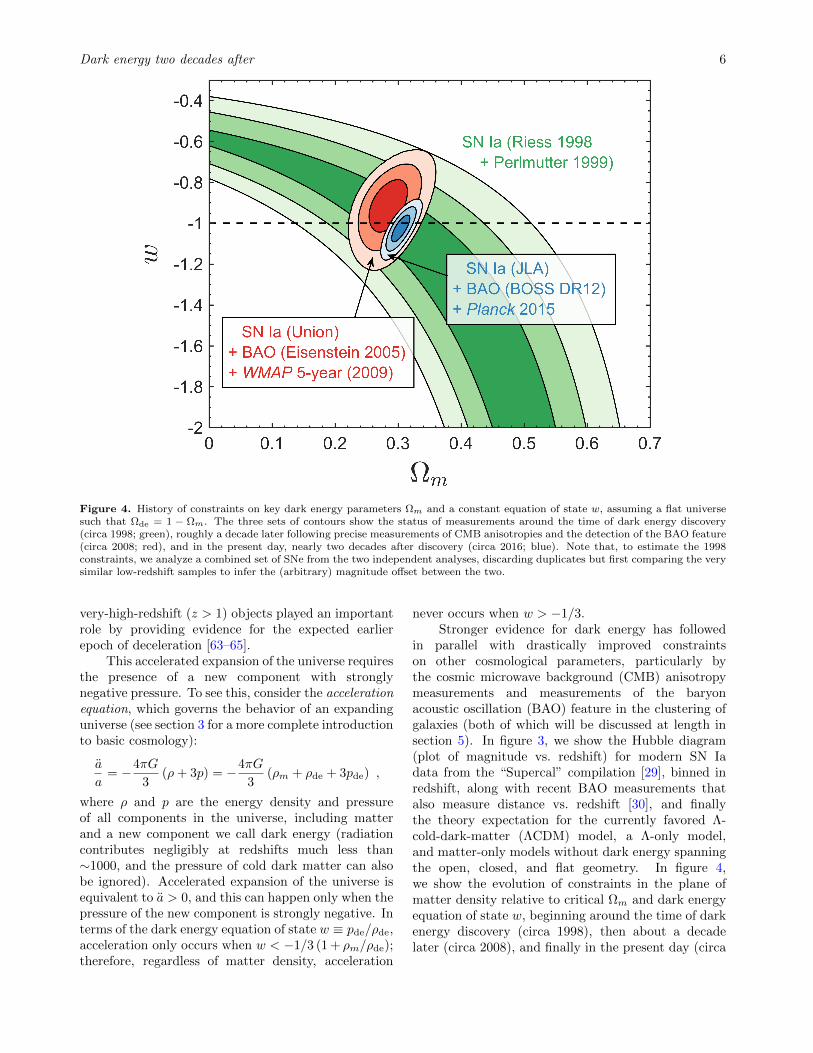
Figure 4. History of constraints on key dark energy parameters Ωm and a constant equation of state w, assuming a flat universesuch that Ωde = 1 − Ωm. The three sets of contours show the status of measurements around the time of dark energy discovery(circa 1998; green), roughly a decade later following precise measurements of CMB anisotropies and the detection of the BAO feature(circa 2008; red), and in the present day, nearly two decades after discovery (circa 2016; blue). Note that, to estimate the 1998constraints, we analyze a combined set of SNe from the two independent analyses, discarding duplicates but first comparing the verysimilar low-redshift samples to infer the (arbitrary) magnitude offset between the two.
very-high-redshift (z > 1) objects played an importantrole by providing evidence for the expected earlierepoch of deceleration [63–65].
This accelerated expansion of the universe requiresthe presence of a new component with stronglynegative pressure. To see this, consider the accelerationequation, which governs the behavior of an expandinguniverse (see section 3 for a more complete introductionto basic cosmology):
a
a= −4πG
3(ρ+ 3p) = −4πG
3(ρm + ρde + 3pde) ,
where ρ and p are the energy density and pressureof all components in the universe, including matterand a new component we call dark energy (radiationcontributes negligibly at redshifts much less than∼1000, and the pressure of cold dark matter can alsobe ignored). Accelerated expansion of the universe isequivalent to a > 0, and this can happen only when thepressure of the new component is strongly negative. Interms of the dark energy equation of state w ≡ pde/ρde,acceleration only occurs when w < −1/3 (1 + ρm/ρde);therefore, regardless of matter density, acceleration
never occurs when w > −1/3.Stronger evidence for dark energy has followed
in parallel with drastically improved constraintson other cosmological parameters, particularly bythe cosmic microwave background (CMB) anisotropymeasurements and measurements of the baryonacoustic oscillation (BAO) feature in the clustering ofgalaxies (both of which will be discussed at length insection 5). In figure 3, we show the Hubble diagram(plot of magnitude vs. redshift) for modern SN Iadata from the “Supercal” compilation [29], binned inredshift, along with recent BAO measurements thatalso measure distance vs. redshift [30], and finallythe theory expectation for the currently favored Λ-cold-dark-matter (ΛCDM) model, a Λ-only model,and matter-only models without dark energy spanningthe open, closed, and flat geometry. In figure 4,we show the evolution of constraints in the plane ofmatter density relative to critical Ωm and dark energyequation of state w, beginning around the time of darkenergy discovery (circa 1998), then about a decadelater (circa 2008), and finally in the present day (circa
Dark energy two decades after 7
2016), nearly two decades later.The discovery of the accelerating universe via SN
Ia observations was a dramatic event that, almostovernight, overturned the previously favored matter-only universe and pointed to a new cosmologicalstandard model dominated by a negative-pressurecomponent. This component that causes the expansionof the universe to accelerate was soon named “darkenergy” by cosmologist Michael Turner [66]. Thephysical nature of dark energy is currently unknown,and the search for it is the subject of worldwideresearch that encompasses theory, observation, andperhaps even laboratory experiments. The physicsbehind dark energy has connections to fundamentalphysics, to astrophysical observations, and to theultimate fate of the universe.
3. Modern cosmology: the basics
We will begin with a brief overview of the physicalfoundations of modern cosmology.
The cosmological principle states that, on largeenough scales, the universe is homogeneous (the sameeverywhere) and isotropic (no special direction). Itis an assumption but also a testable hypothesis,and indeed there is excellent observational evidencethat the universe satisfies the cosmological principleon its largest spatial scales (e.g. [67, 68]). Underthese assumptions, the metric can be written in theRobertson-Walker (RW) form
ds2 = dt2 − a2(t)
[dr2
1− kr2+ r2
(dθ2 + sin2 θ dφ2
)],
where r, θ, and φ are comoving spatial coordinates, tis time, and the expansion is described by the cosmicscale factor a(t), where the present value is a(t0) = 1 byconvention. The quantity k is the intrinsic curvatureof three-dimensional space; k = 0 corresponds to aspatially flat universe with Euclidean geometry, whilek > 0 corresponds to positive curvature (sphericalgeometry) and k < 0 to negative curvature (hyperbolicgeometry).
The scale factor a(t) is a function of the energydensities and pressures of the components that fill theuniverse. Its evolution is governed by the Friedmannequations, which are derived from Einstein’s equationsof general relativity using the RW metric:
H2 ≡(a
a
)2
=8πGρ
3− k
a2+
Λ
3, (1)
a
a= −4πG
3(ρ+ 3p) +
Λ
3, (2)
whereH is the Hubble parameter, Λ is the cosmologicalconstant term, ρ is the total energy density, and p is the
pressure. Note that the cosmological constant Λ can besubsumed into the energy density ρ, but separating outΛ reflects how it was incorporated historically, beforethe discovery of the accelerating universe.
We can define the critical density ρcrit ≡3H2/(8πG) as the density that leads to a flat universewith k = 0. Then the effect of dark energy on theexpansion rate can be described by its present-dayenergy density relative to critical Ωde and its equationof state w, which is the ratio of pressure to energydensity:
Ωde ≡ρde,0
ρcrit,0; w ≡ pde
ρde. (3)
The simplest possibility is that the equation of state isconstant in time. This is in fact the case for (cold,nonrelativistic) matter (wmatter = 0) and radiation(wrad = 1/3). However, it is also possible thatw evolves with time (or redshift). The continuityequation,
ρ = −3H(ρ+ p) , (4)
is not an independent result but can be derived from(1) and (2). An expression of conservation of energy,it can used to solve for the dark energy density as afunction of redshift for an arbitrary equation of statew(z):
ρde(z) = ρde,0 exp
[3
∫ z
0
1 + w(z′)
1 + z′dz′]
(5)
= ρde,0 (1 + z)3(1+w),
where the second equality is the simplified result forconstant w.
The expansion rate of the universe H ≡ a/a from(1) can then be written as (again for w = constant)
H2 = H20
[Ωm(1 + z)3 + Ωr(1 + z)4 (6)
+ Ωde(1 + z)3(1+w) + Ωk(1 + z)2],
where H0 is the present value of the Hubble parameter(the Hubble constant), Ωm and Ωr are the matterand radiation energy densities relative to critical, andthe dimensionless curvature “energy density” Ωk isdefined such that
∑i Ωi = 1. Since Ωr ' 8 × 10⁻⁵,
we can typically ignore the radiation contribution forlow-redshift (z . 10) measurements; however, nearthe epoch of recombination (z ∼ 1000), radiationcontributes significantly, and at earlier times (z &3300), it dominates.
3.1. Distances and geometry
Observational cosmology is complicated by the factthat we live in an expanding universe where distances
Dark energy two decades after 8
must be defined carefully. Astronomical observations,including those that provide clues about nature of darkenergy, fundamentally rely on two basic techniques,measuring fluxes from objects and measuring angleson the sky. It is therefore useful to define two typesof distance, the luminosity distance and the angulardiameter distance. The luminosity distance dL is thedistance at which an object with a certain luminosityproduces a certain flux (f = L/(4πd2
L)), while theangular diameter distance dA is the distance at which acertain (transverse) physical separation xtrans producesa certain angle on the sky (θ = xtrans/dA). Fora (homogeneous and isotropic) Friedmann-Robertson-Walker universe, the two are closely related and givenin terms of the comoving distance r(z):
dL(z) = (1 + z) r(z) ; dA(z) =1
1 + zr(z) . (7)
The comoving distance can be written compactly as
r(z) = limΩ′k→Ωk
c
H0
√Ω′k
sinh
[√Ω′k
∫ z
0
H0
H(z′)dz′],
(8)which is valid for all Ωk (positive, negative, zero) andwhere H(z) is the Hubble parameter (e.g. (6)).
Having specified the effect of dark energy onthe expansion rate and the distances, its effect onany quantity that fundamentally only depends on theexpansion rate can be computed. For example, numbercounts of galaxy clusters are sensitive to the volumeelement of the universe, given by
dV
dz dΩ=
r2(z)
H(z)/c,
where dz and dΩ are the redshift and solid angleintervals, respectively. Similarly, some methods rely onmeasuring ages of galaxies, which requires knowledgeof the age-redshift relation. The age of the universe foran arbitrary scale factor a = 1/(1 + z) is given by
t(a) =
∫ a
0
da′
a′H(a′).
We will make one final point here. Noticefrom (8) that, when calculating distance, the darkenergy parameters Ωde and w are hidden behindan integral (and behind two integrals when ageneral w(z) is considered; see (5)). The Hubbleparameter H(z) is in the integrand of the distanceformula and therefore requires one fewer integralto calculate; it depends more directly on the darkenergy parameters. Therefore, direct measurements ofthe Hubble parameter, or of quantities that dependdirectly on H(z), are nominally more sensitive to darkenergy than observables that fundamentally dependon distance. Unfortunately, measurements of H(z)
are more difficult to achieve and/or are inferredsomewhat indirectly, such as from differential distancemeasurements.
3.2. Density fluctuations
Next we turn to the growth of matter densityfluctuations, δ ≡ δρm/ρm. Assuming that generalrelativity holds, and assuming small matter densityfluctuations |δ| 1 on length scales much smallerthan the Hubble radius, the temporal evolution of thefluctuations is given by
δk + 2Hδk − 4πGρmδk = 0 , (9)
where δk is the Fourier component§ corresponding tothe mode with wavenumber k ' 2π/λ. In (9), darkenergy enters twofold: in the friction term, where itaffects H; and in the source term, where it reducesρm. For H(z) normalized at high redshift, dark energyincreases the expansion rate at z . 1, stunting thegrowth of density fluctuations.
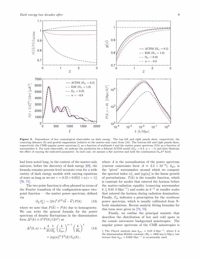
The effect of dark energy on growth is illustratedin the top right panel of figure 5, where we show thegrowth-suppression factor g(z), which indicates theamount of growth relative to that in an Einstein-deSitter universe, which contains no dark energy. Itis implicitly defined with respect to the scaled lineargrowth of fluctuations,
D(a) ≡ δ(a)
δ(1)≡ a g(a)
g(1). (10)
With only matter, D(a) = a and g(a) = 1 at all times.In the presence of dark energy, g(a) falls below unityat late times. In the currently favored ΛCDM model,g(1) ' 0.78. The value of the density fluctuationδ at scale factor a, relative to the matter-only case,is suppressed by a factor g(a), while the two-pointcorrelation function is suppressed by g2.
A useful alternative expression for the growthsuppression is
g(a) = exp
[∫ a
0
da′
a′(f(a′)− 1)
], (11)
where
f(a) ≡ d lnD
d ln a≈ Ωm(a)γ (12)
is the growth rate which, as we will see below,contains very important sensitivity to both dark energyparameters and to modifications to gravity. The latter,approximate equality in (12) is remarkably accurateprovided γ ' 0.55. While this functional form for f(a)
§ Given our assumptions, each wavenumber evolves indepen-dently, though this does not always hold for modified theoriesof gravity, even in linear theory.
Dark energy two decades after 9
0 1 2 3
0.7
0.8
0.9
1
1.1
0 1 2 30.7
0.8
0.9
1
0 500 1000 1500 20000
1000
2000
3000
4000
5000
6000
7000
10-4
10-3
10-2
10-1
100
102
103
104
Figure 5. Dependence of key cosmological observables on dark energy. The top left and right panels show, respectively, thecomoving distance (8) and growth suppression (relative to the matter-only case) from (10). The bottom left and right panels show,respectively, the CMB angular power spectrum C` as a function of multipole ` and the matter power spectrum P (k) as a function ofwavenumber k. For each observable, we indicate the prediction for a fiducial ΛCDM model (Ωm = 0.3, w = −1) and then illustratethe effect of varying the indicated parameter. In each case, we assume a flat universe and hold the combination Ωmh2 fixed.
had been noted long, in the context of the matter-onlyuniverse, before the discovery of dark energy [69], theformula remains percent-level accurate even for a widevariety of dark energy models with varying equationsof state as long as we set γ = 0.55 + 0.05[1 +w(z = 1)][70, 71].
The two point function is often phrased in terms ofthe Fourier transform of the configuration-space two-point function — the matter power spectrum, definedvia
〈δ~k δ∗~k′〉 = (2π)3 δ(3)(~k − ~k′)P (k) (13)
where we note that P (~k) = P (k) due to homogeneity.We can write the general formula for the powerspectrum of density fluctuations in the dimensionlessform ∆2(k) ≡ k3P (k)/(2π2) as
∆2(k, a) = A4
25
1
Ω2m
(k
kpiv
)n−1(k
H0
)4
(14)
× [ag(a)]2 T 2(k)Tnl(k) ,
where A is the normalization of the power spectrum(current constraints favor A ≈ 2.2 × 10⁻⁹), kpiv isthe “pivot” wavenumber around which we computethe spectral index n‖, and [ag(a)] is the linear growthof perturbations. T (k) is the transfer function, whichis constant for modes that entered the horizon beforethe matter-radiation equality (comoving wavenumberk . 0.01 hMpc−1) and scales as k−2 at smaller scalesthat entered the horizon during radiation domination.Finally, Tnl indicates a prescription for the nonlinearpower spectrum, which is usually calibrated from N-body simulations. Recent analytic fitting formulae forthis term were given in [72, 73].
Finally, we outline the principal statistic thatdescribes the distribution of hot and cold spots inthe cosmic microwave background anisotropies. Theangular power spectrum of the CMB anisotropies is
‖ The Planck analysis uses kpiv = 0.05 hMpc−1, where h isthe dimensionless Hubble constant (H0 = 100h km/s/Mpc), butbeware that kpiv = 0.002 Mpc−1 is occasionally used.
Dark energy two decades after 10
essentially a projection along the line of sight of theprimordial matter power spectrum. Adopting theexpansion of the temperature anisotropies on the skyin terms of the complex coefficients a`m,
δT
T(n) =
∞∑`=2
∑m=−`
a`m Y`m(n) , (15)
we can obtain the ensemble average of the two pointcorrelation function of the coefficients C` ≡ 〈|a`m|2〉 as
C` = 4π
∫∆2(k)j2
` (kr∗)d ln k ,
where j` is the spherical bessel function and r∗ is theradius of the sphere onto which we are projecting (thecomoving distance to recombination); in the standardmodel, r∗ ' 14.4 Gpc. Physical structures that appearat angular separations θ roughly correspond to powerat multipole ` ' π/θ.
Basic observables and their variation when a fewbasic parameters governing dark energy are varied areshown in figure 5. To illustrate the effects of variationsin the dark energy model, we compare the followingfour models:
(i) Flat model with matter density Ωm = 0.3,equation of state w = −1, and other parametersin agreement with the most recent cosmologicalconstraints [74].
(ii) Same as (i), but with Ωm = 1. This isthe Einstein-de Sitter model, flat and matterdominated with no dark energy. We hold all otherparameters, including the combination Ωmh
2,fixed to their best-fit values in (i).
(iii) Same as (i), except Ωm = 0.25.
(iv) Same as (i), but with w = −0.8.
4. Parametrizations of dark energy
4.1. Introduction
Given the lack of a consensus model for cosmicacceleration, it is a challenge to provide a simpleyet unbiased and sufficiently general descriptionof dark energy. The equation-of-state parameterw has traditionally been identified as one usefulphenomenological description; being the ratio ofpressure to energy density, it is also closely connectedto the underlying physics. Many more generalparametrizations exist, some of them with appealingstatistical properties. We now review a variety offormalisms that have been used to describe andconstrain dark energy.
We first describe parametrizations used to de-scribe the effects of dark energy on observable quanti-ties. We then discuss the reconstruction of the dark-energy history; the principal-component description of
it; the figures of merit; and descriptions of more gen-eral possibilities beyond spatially smooth dark energy,including modified gravity models. We end by outlin-ing two strategies to test the internal consistency of thecurrently favored ΛCDM model.
4.2. Parametrizations
Assuming that dark energy is spatially smooth, itssimplest parametrization is in terms of its equation-of-state [75, 76]
w ≡ pde
ρde= constant. (16)
This form describes vacuum energy (w = −1) andtopological defects (w = −N/3, where N is theinteger dimension of the defect and takes the value0, 1, or 2 for monopoles, cosmic strings, or textures,respectively). Together with Ωde, w provides atwo-parameter description of the dark-energy sector.However, it does not describe models which have atime-varying w, such as scalar field dark energy ormodified gravity, although cosmological observablesare often sufficiently accurately described by a constantw even for models with mildly varying w(z).
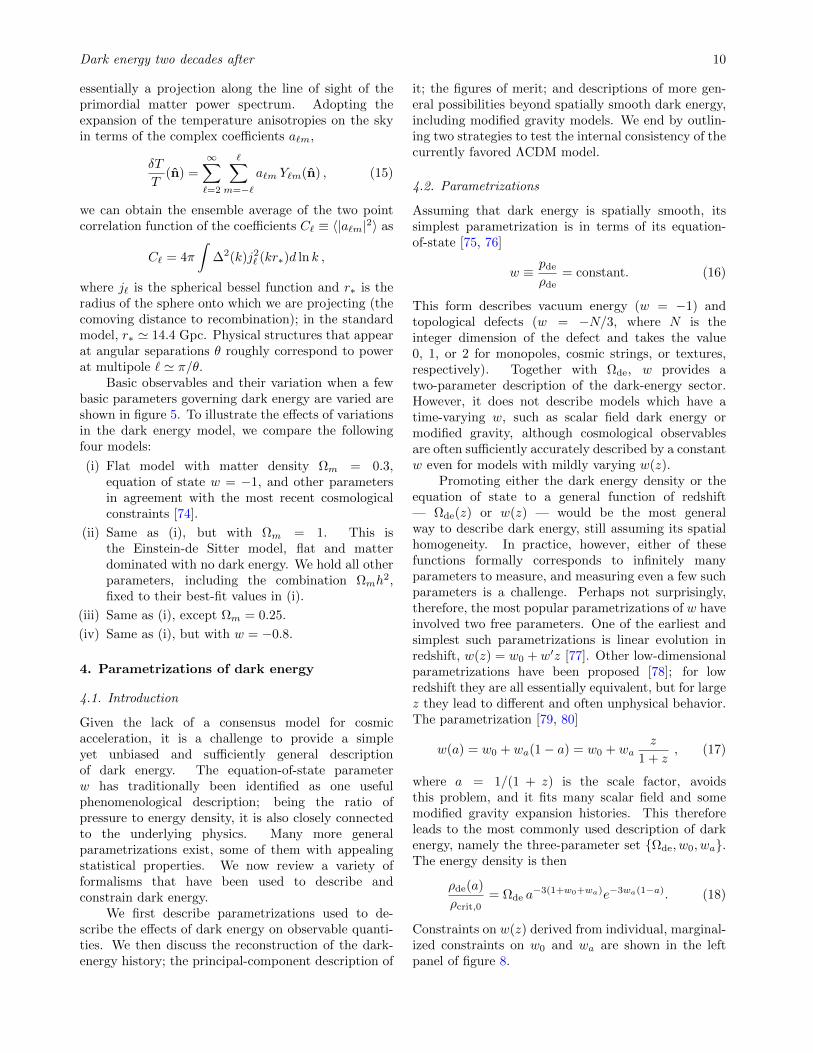
Promoting either the dark energy density or theequation of state to a general function of redshift— Ωde(z) or w(z) — would be the most generalway to describe dark energy, still assuming its spatialhomogeneity. In practice, however, either of thesefunctions formally corresponds to infinitely manyparameters to measure, and measuring even a few suchparameters is a challenge. Perhaps not surprisingly,therefore, the most popular parametrizations of w haveinvolved two free parameters. One of the earliest andsimplest such parametrizations is linear evolution inredshift, w(z) = w0 + w′z [77]. Other low-dimensionalparametrizations have been proposed [78]; for lowredshift they are all essentially equivalent, but for largez they lead to different and often unphysical behavior.The parametrization [79, 80]
w(a) = w0 + wa(1− a) = w0 + waz
1 + z, (17)
where a = 1/(1 + z) is the scale factor, avoidsthis problem, and it fits many scalar field and somemodified gravity expansion histories. This thereforeleads to the most commonly used description of darkenergy, namely the three-parameter set Ωde, w0, wa.The energy density is then
ρde(a)
ρcrit,0= Ωde a
−3(1+w0+wa)e−3wa(1−a). (18)
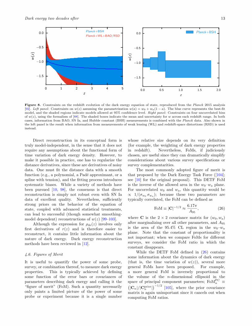
Constraints on w(z) derived from individual, marginal-ized constraints on w0 and wa are shown in the leftpanel of figure 8.
Dark energy two decades after 11
More general expressions have been proposed (e.g.[81, 82]); however, introducing additional parametersmakes the equation of state very difficult to measure,and such extra parameters are often ad hoc andunmotivated from either a theoretical or empiricalpoint of view.
4.3. Pivot redshift
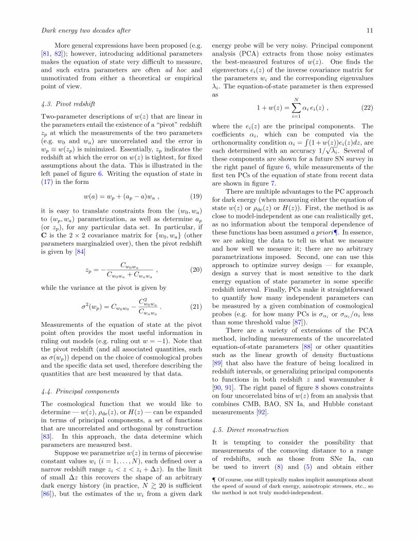
Two-parameter descriptions of w(z) that are linear inthe parameters entail the existence of a “pivot” redshiftzp at which the measurements of the two parameters(e.g. w0 and wa) are uncorrelated and the error inwp ≡ w(zp) is minimized. Essentially, zp indicates theredshift at which the error on w(z) is tightest, for fixedassumptions about the data. This is illustrated in theleft panel of figure 6. Writing the equation of state in(17) in the form
w(a) = wp + (ap − a)wa , (19)
it is easy to translate constraints from the (w0, wa)to (wp, wa) parametrization, as well as determine ap(or zp), for any particular data set. In particular, ifC is the 2 × 2 covariance matrix for w0, wa (otherparameters marginalzied over), then the pivot redshiftis given by [84]
zp = − Cw0wa
Cw0wa + Cwawa, (20)
while the variance at the pivot is given by
σ2(wp) = Cw0w0−C2w0wa
Cwawa. (21)
Measurements of the equation of state at the pivotpoint often provides the most useful information inruling out models (e.g. ruling out w = −1). Note thatthe pivot redshift (and all associated quantities, suchas σ(wp)) depend on the choice of cosmological probesand the specific data set used, therefore describing thequantities that are best measured by that data.
4.4. Principal components
The cosmological function that we would like todetermine — w(z), ρde(z), or H(z) — can be expandedin terms of principal components, a set of functionsthat are uncorrelated and orthogonal by construction[83]. In this approach, the data determine whichparameters are measured best.
Suppose we parametrize w(z) in terms of piecewiseconstant values wi (i = 1, . . . , N), each defined over anarrow redshift range zi < z < zi + ∆z). In the limitof small ∆z this recovers the shape of an arbitrarydark energy history (in practice, N & 20 is sufficient[86]), but the estimates of the wi from a given dark
energy probe will be very noisy. Principal componentanalysis (PCA) extracts from those noisy estimatesthe best-measured features of w(z). One finds theeigenvectors ei(z) of the inverse covariance matrix forthe parameters wi and the corresponding eigenvaluesλi. The equation-of-state parameter is then expressedas
1 + w(z) =
N∑i=1
αi ei(z) , (22)
where the ei(z) are the principal components. Thecoefficients αi, which can be computed via theorthonormality condition αi =
∫(1 +w(z))ei(z)dz, are
each determined with an accuracy 1/√λi. Several of
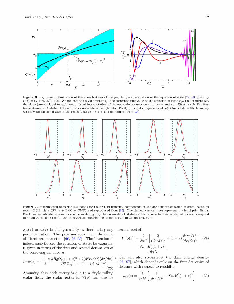
these components are shown for a future SN survey inthe right panel of figure 6, while measurements of thefirst ten PCs of the equation of state from recent dataare shown in figure 7.
There are multiple advantages to the PC approachfor dark energy (when measuring either the equation ofstate w(z) or ρde(z) or H(z)). First, the method is asclose to model-independent as one can realistically get,as no information about the temporal dependence ofthese functions has been assumed a priori¶. In essence,we are asking the data to tell us what we measureand how well we measure it; there are no arbitraryparametrizations imposed. Second, one can use thisapproach to optimize survey design — for example,design a survey that is most sensitive to the darkenergy equation of state parameter in some specificredshift interval. Finally, PCs make it straightforwardto quantify how many independent parameters canbe measured by a given combination of cosmologicalprobes (e.g. for how many PCs is σαi or σαi/αi lessthan some threshold value [87]).
There are a variety of extensions of the PCAmethod, including measurements of the uncorrelatedequation-of-state parameters [88] or other quantitiessuch as the linear growth of density fluctuations[89] that also have the feature of being localized inredshift intervals, or generalizing principal componentsto functions in both redshift z and wavenumber k[90, 91]. The right panel of figure 8 shows constraintson four uncorrelated bins of w(z) from an analysis thatcombines CMB, BAO, SN Ia, and Hubble constantmeasurements [92].
4.5. Direct reconstruction
It is tempting to consider the possibility thatmeasurements of the comoving distance to a rangeof redshifts, such as those from SNe Ia, canbe used to invert (8) and (5) and obtain either
¶ Of course, one still typically makes implicit assumptions aboutthe speed of sound of dark energy, anisotropic stresses, etc., sothe method is not truly model-independent.
Dark energy two decades after 12
0 0.1 0.2 0.3 0.4z
w
2σ(wp)
σ(w0)
wp
zp
w0
slope = wa/(1+z)2
0 0.5 1 1.5z
-0.5
0
0.5
e i(z)
1
2
3
4
49
50
Figure 6. Left panel : Illustration of the main features of the popular parametrization of the equation of state [79, 80] given byw(z) = w0 + wa z/(1 + z). We indicate the pivot redshift zp, the corresponding value of the equation of state wp, the intercept w0,the slope (proportional to wa), and a visual interpretation of the approximate uncertainties in w0 and wp. Right panel : The fourbest-determined (labeled 1–4) and two worst-determined (labeled 49-50) principal components of w(z) for a future SN Ia surveywith several thousand SNe in the redshift range 0 < z < 1.7; reproduced from [83].
1 0 1α1
1 0 1α2
1 0 1α3
1 0 1α4
1 0 1α5
1 0 1α6
1 0 1α7
1 0 1α8
1 0 1α9
1 0 1α10
Figure 7. Marginalized posterior likelihoods for the first 10 principal components of the dark energy equation of state, based onrecent (2012) data (SN Ia + BAO + CMB) and reproduced from [85]. The dashed vertical lines represent the hard prior limits.Black curves indicate constraints when considering only the uncorrelated, statistical SN Ia uncertainties, while red curves correspondto an analysis using the full SN Ia covariance matrix, including all systematic uncertainties.
ρde(z) or w(z) in full generality, without using anyparametrization. This program goes under the nameof direct reconstruction [66, 93–95]. The inversion isindeed analytic and the equation of state, for example,is given in terms of the first and second derivatives ofthe comoving distance as
1+w(z) =1 + z
3
3H20 Ωm(1 + z)2 + 2(d2r/dz2)(dr/dz)−3
H20 Ωm(1 + z)3 − (dr/dz)−2
.
(23)Assuming that dark energy is due to a single rollingscalar field, the scalar potential V (φ) can also be
reconstructed.
V [φ(z)] =1
8πG
[3
(dr/dz)2+ (1 + z)
d2r/dz2
(dr/dz)3
](24)
− 3ΩmH20 (1 + z)3
16πG.
One can also reconstruct the dark energy density[96, 97], which depends only on the first derivative ofdistance with respect to redshift,
ρde(z) =3
8πG
[1
(dr/dz)2− ΩmH
20 (1 + z)3
]. (25)
Dark energy two decades after 13
0 1 2 3 4 5
z
−1.5
−1.0
−0.5
0.0w
(z)
Planck+BSH
Planck+WL+BAO/RSD
0.0 0.5 1.0 1.5 2.0
z
1.5
1.0
0.5
0.0
w(z
)
Planck+BSH
0.0 0.5 1.0 1.5 2.0
z
0.0
0.2
0.4
0.6
0.8
1.0
Wei
ght
bin 0
bin 1
bin 2
bin 3
Figure 8. Constraints on the redshift evolution of the dark energy equation of state, reproduced from the Planck 2015 analysis[92]. Left panel : Constraints on w(z) assuming the parametrization w(a) = w0 + wa(1− a). The blue curve represents the best-fitmodel, and the shaded regions indicate models allowed at 95% confidence level. Right panel : Constraints on four uncorrelated binsof w(z), using the formalism of [88]. The shaded boxes indicate the mean and uncertainty for w across each redshift range. In bothcases, information from BAO, SN Ia, and Hubble constant (BSH) measurements is combined with the Planck data. Also shown inthe left panel is the result when information from measurements of weak lensing (WL) and redshift-space distortions (RSD) is usedinstead.
Direct reconstruction in its conceptual form istruly model-independent, in the sense that it does notrequire any assumptions about the functional form oftime variation of dark energy density. However, tomake it possible in practice, one has to regularize thedistance derivatives, since these are derivatives of noisydata. One must fit the distance data with a smoothfunction (e.g., a polynomial, a Pade approximant, or aspline with tension), and the fitting process introducessystematic biases. While a variety of methods havebeen pursued [10, 98], the consensus is that directreconstruction is simply not robust even with SN Iadata of excellent quality. Nevertheless, sufficientlystrong priors on the behavior of the equation ofstate, coupled with advanced statistical treatments,can lead to successful (though somewhat smoothing-model dependent) reconstructions of w(z) [99–103].
Although the expression for ρde(z) involves onlyfirst derivatives of r(z) and is therefore easier toreconstruct, it contains little information about thenature of dark energy. Dark energy reconstructionmethods have been reviewed in [12].
4.6. Figures of Merit
It is useful to quantify the power of some probe,survey, or combination thereof, to measure dark energyproperties. This is typically achieved by definingsome function of the error bars or covariances ofparameters describing dark energy and calling it the“figure of merit” (FoM). Such a quantity necessarilyonly paints a limited picture of the power of someprobe or experiment because it is a single number
whose relative size depends on its very definition(for example, the weighting of dark energy propertiesin redshift). Nevertheless, FoMs, if judiciouslychosen, are useful since they can dramatically simplifyconsiderations about various survey specifications orsurvey complementarities.
The most commonly adopted figure of merit isthat proposed by the Dark Energy Task Force ([104];see [10] for the original proposal). This DETF FoMis the inverse of the allowed area in the w0–wa plane.For uncorrelated w0 and wa, this quantity would be∝ 1/(σw0
σwa); because these two parameters aretypically correlated, the FoM can be defined as
FoM ≡ |C|−1/2 ≈ 6.17π
A95, (26)
where C is the 2 × 2 covariance matrix for (w0, wa)after marginalizing over all other parameters, and A95
is the area of the 95.4% CL region in the w0–waplane. Note that the constant of proportionality isnot important; when we compare FoMs for differentsurveys, we consider the FoM ratio in which theconstant disappears.
While the DETF FoM defined in (26) containssome information about the dynamics of dark energy(that is, the time variation of w(z)), several moregeneral FoMs have been proposed. For example,a more general FoM is inversely proportional tothe volume of the n-dimensional ellipsoid in thespace of principal component parameters; FoMPC
n ≡(|Cn|/|Cprior
n |)−1/2
[105], where the prior covariancematrix is again unimportant since it cancels out whencomputing FoM ratios.
Dark energy two decades after 14
4.7. Generalized dark energy phenomenology
The simplest and by far the most studied class ofmodels is dark energy that is spatially smooth and itsonly degree of freedom is its energy density — that is, itis fully described by either ρde(a) or w(a) ∼ −1. Moregeneral possibilities exist however, as the stress-energytensor allows considerably more freedom [106, 107].
One possibility is that dark energy has the speed ofsound that allows clustering at sub-horizon scales, thatis, c2s ≡ δpde/δρde < 1 (where cs is quoted in units ofthe speed of light) [108–111]. Unfortunately, the effectsof the speed of sound are small, and become essentiallynegligible in the limit when the equation of state ofdark energy w becomes close to −1, and are difficultto discern with late-universe measurements even if wdeviates from the cosmological constant value at someepoch. It will therefore be essentially impossible tomeasure the speed of sound even with future surveys;see illustrations of the changes in the observables andforecasts in [112].
Another possibility is the presence of “early darkenergy” [113–115], component that is non-negligible atearly times, typically around recombination or evenearlier. The early component is motivated by varioustheoretical models (e.g. scalar fields [116]), and couldimprint signatures via the early-time Integrated Sachs-Wolfe effect. While the acceleration in the redshiftrange z ∈ [1, 105] is already ruled out [117], oforder a percent contribution to the energy budget byearly dark energy is still allowed [92, 118]. In somemodels, this early component this component acts likeradiation in the early universe [119]. Increasingly goodconstraints on models with early dark energy are onthe to-do list for upcoming cosmological probes.
Finally, there is a possibility that dark energyis coupled to dark matter, or other components orparticles (some of the early work is in e.g. [120–122]). This is a much richer — though typically verymodel-dependent — set of possibilities, with manyopportunities to test them using data; see [123] for areview.
As yet, there is no observational evidencefor generalized dark energy beyond the simplestmodel but, as with modified gravity, studying theseextensions is important to understand how dark energyphenomenology can be searched for by cosmologicalprobes.
4.8. Descriptions of modified gravity
Modifications of General Theory of relativity representa fundamental alternative in describing the apparentacceleration to the smooth fluid description witha negative equation of state. In modified gravity(reviewed in this volume by P. Brax), the modification
of GR makes an order-unity change in the dynamicsat cosmological scales. At the solar-system scales, themodification of gravity needs to have a very smallor negligible effect — usually satisfied by invokingnon-linear “screening mechanisms” which restore GRin high density regions — in order to respect thesuccessful local tests of GR. There exists a diverseset of proposed modified gravity theories, with veryrich set of potentially new cosmological signatures; forexcellent reviews, see [124–126].
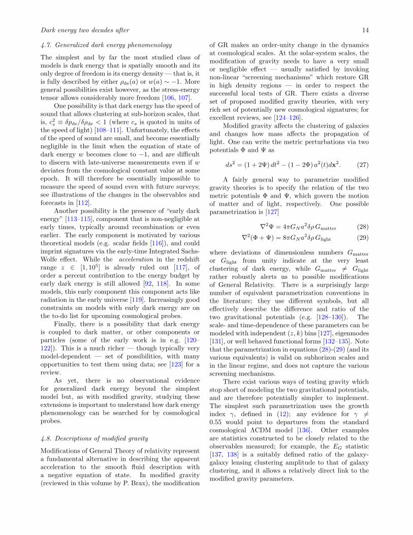
Modified gravity affects the clustering of galaxiesand changes how mass affects the propagation oflight. One can write the metric perturbations via twopotentials Φ and Ψ as
ds2 = (1 + 2Ψ) dt2 − (1− 2Φ) a2(t)dx2. (27)
A fairly general way to parametrize modifiedgravity theories is to specify the relation of the twometric potentials Φ and Ψ, which govern the motionof matter and of light, respectively. One possibleparametrization is [127]
∇2Ψ = 4πGNa2δρGmatter (28)
∇2(Φ + Ψ) = 8πGNa2δρGlight (29)
where deviations of dimensionless numbers Gmatter
or Glight from unity indicate at the very leastclustering of dark energy, while Gmatter 6= Glight
rather robustly alerts us to possible modificationsof General Relativity. There is a surprisingly largenumber of equivalent parametrization conventions inthe literature; they use different symbols, but alleffectively describe the difference and ratio of thetwo gravitational potentials (e.g. [128–130]). Thescale- and time-dependence of these parameters can bemodeled with independent (z, k) bins [127], eigenmodes[131], or well behaved functional forms [132–135]. Notethat the parametrization in equations (28)-(29) (and itsvarious equivalents) is valid on subhorizon scales andin the linear regime, and does not capture the variousscreening mechanisms.
There exist various ways of testing gravity whichstop short of modeling the two gravitational potentials,and are therefore potentially simpler to implement.The simplest such parametrization uses the growthindex γ, defined in (12); any evidence for γ 6=0.55 would point to departures from the standardcosmological ΛCDM model [136]. Other examplesare statistics constructed to be closely related to theobservables measured; for example, the EG statistic[137, 138] is a suitably defined ratio of the galaxy-galaxy lensing clustering amplitude to that of galaxyclustering, and it allows a relatively direct link to themodified gravity parameters.

Dark energy two decades after 15
4.9. Consistency tests of the standard model
Finally, there are powerful but more phenomenolog-ical methods of testing the consistency of the cur-rent cosmological model that do not refer to explicitparametrizations of modified gravity theory. The gen-eral idea behind such tests is to begin with somewidely adopted parametrization of the cosmologicalmodel (say, the ∼5-parameter ΛCDM), then investi-gate whether there exist observations that are incon-sistent with the theoretical predictions of the model.Bayesian statistical tools [139–145] are particularlyuseful to quantify these consistency tests.
The simplest approach is to calculate predictionson cosmological functions that can be measured thatare consistent with current parameter constraints [86,146, 147]. The predictions depend on the classof models that one is trying to test; for example,predictions for weak lensing shear power spectrum thatassume an underlying ΛCDM model are tighter thanthe weak-lensing predictions that assume an evolvingscalar field model where the equation of state ofdark energy is a free function of time. Such model-dependent predictions for the observed quantities arenow routinely employed in cosmological data analysis,as they provide a useful check of whether the newlyobtained data fall within those predictions (e.g. [30]).
A complementary approach is to explicitly splitthe cosmological parameters into those constrained bygeometry (e.g, distances, as in SNIa and BAO), andthose constrained by the growth of structure (e.g. theevolution of clustering amplitude in redshift) [148–150]. In this approach, the equation of state of darkenergy w, for example, can be split into two separateparameters, wgeom and wgrow. These two parametersare then employed in those terms in theory equationsthat are based on geometry and growth, respectively.In this scheme, the principal hypothesis being testedis whether wgeom = wgrow. This so-called growth-geometry split allows explicit insights into what thedata is telling us in case there is tension with ΛCDM,as this currently favored model makes very precisepredictions about the relation between the growthand geometry quantities. For example, the currentlydiscussed discrepancy between the measurement ofthe amplitude of mass fluctuations between the CMBand weak lensing (e.g. [151]) can be understood moreclearly as the fact that the growth of structure —from current data, and not (yet) at an overwhelmingstatistical significance — is even more suppressedthan predicted in the standard cosmological model,as the geometry-growth analysis indicates [152, 153].Future cosmological constraints that incorporate animpressive range of probes with complementary physicssensitive to dark energy will be a particularly good testbed for the geometry-growth split analyses.
5. Principal probes of dark energy
In this section, we review the classic, principalcosmological probes of dark energy. What criterionmakes a probe ’primary’ is admittedly somewhatarbitrary; here we single out and describe the mostmature probes of dark energy: type Ia supernovae(SNe Ia), the baryon acoustic oscillations (BAO), thecosmic microwave background (CMB), weak lensing,and galaxy clusters. We briefly review the history ofthese probes and discuss their current status and futurepotential. In the following section (section 6), we willdiscuss other probes of dark energy. Finally, in Table1 we summarize the primary and secondary probes ofdark energy, along with their principal strengths andweaknesses.
5.1. Type Ia supernovae
Type Ia supernovae (SNe Ia) are very bright standardcandles (sometimes called standardizable candles)useful for measuring cosmological distances. Below wediscuss why standard candles are useful and then goon to review cosmology with SNe Ia, including a briefdiscussion of systematic errors and recent progress.
5.1.1. Standard candles. Distances in astronomy areoften notoriously difficult to measure. It is relativelystraightforward to measure the angular location ofan object in the sky, and we can often obtain aprecise measurement of an object’s redshift z fromits spectrum by observing the shift of known spectrallines due to the expansion of the universe (1 + z ≡λobs/λemit). For a specified cosmological model, thedistance-redshift relation (i.e. (8)) would then indicatethe distance; however, since our goal is typically toinfer the cosmological model, we need an independentdistance measurement. Methods of independentlymeasuring distance in astronomy typically involveuncertain empirical relationships. To measure the(absolute) distance to an object, such as a galaxy,astronomers have to construct a potentially unwieldy“distance ladder.” For instance, they may employrelatively direct parallax measurements (apparentshifts due to Earth’s motion around the Sun) tomeasure distances to nearby objects in our galaxy(e.g. Cepheid variable stars), then use those objectsto measure distances to other nearby galaxies (forCepheids, the empirical relation between pulsationperiod and intrinsic luminosity is the key). Ifsystematic errors add up at each rung, the distanceladder will become flimsy.
Standard candles are idealized objects that have afixed intrinsic luminosity or absolute magnitude [154].Having standard candles would be very useful; theywould allow us to infer distances to those objects

Dark energy two decades after 16
using only the inverse square law for flux (recall thatf = L/(4πd2
L), where dL is the luminosity distance). Infact, we do not even need to know the luminosity of thestandard candle when determining relative distancesfor a set of objects is sufficient. Observationally, fluxis typically quantified logarithmically (the apparentmagnitude), while luminosity is related to the absolutemagnitude of the object. We therefore have therelation
m−M = 5 log10
(dL
10 pc
), (30)
where the quantity m −M is known as the distancemodulus. For an object that is 10 pc away, the distancemodulus is zero. For a true standard candle, theabsolute magnitude M is the same for each object.Therefore, for each object, a measurement of theapparent magnitude provides direct information aboutthe luminosity distance and therefore some informationabout the cosmological model.
5.1.2. Cosmology with SNe Ia. Supernovae areenergetic stellar explosions, often visible from distantcorners of the universe. Unlike other types ofsupernovae, which result from the core collapseof a massive, dying star, a type Ia supernova isthought to occur when a slowly rotating carbon-oxygen white dwarf accretes matter from a companionstar, eventually exceeds the Chandrasekhar mass limit(∼1.4M), and subsequently collapses and explodes+.The empirical SN classification scheme is based onspectral features, and type Ia SNe are characterizedby a lack of hydrogen lines and the presence of a singlyionized silicon (Si II) line at 6150 A. The flux of lightfrom SNe Ia increases and then fades over a periodof about a month; at its peak flux, a SN can be asluminous as the entire galaxy in which it resides.
SNe Ia had been studied extensively by FritzZwicky (e.g. [157]), who gave them their name andnoted that SNe Ia have roughly uniform luminosities.The fact that SNe Ia can potentially be used asstandard candles had been realized long ago, at leastsince the 1970s [158, 159]. However, developing anobserving strategy to detect SNe Ia before they reachedpeak flux was a major challenge. If we were topoint a telescope at a single galaxy and wait for aSN to occur, we would have to wait ∼100 years, onaverage. A program in the 1980s to find SNe [160]discovered only one, and even then, only after thepeak of the light curve. Today, after many dedicated
+ While a white dwarf is always involved, other details ofthe progenitor system, or of the nuclear ignition and burningmechanism, are far from certain. It seems to be the casethat many SNe Ia result from a merger between two whitedwarfs (double degenerate progenitors), and there may be morediversity in the type of companion star than once thought (e.g.[155, 156]).
observational programs, thousands of SNe Ia have beenobserved, and nearly one thousand have been analyzedsimultaneously for cosmological inference.
Of course, SNe Ia are not perfect standard candles;their peak magnitudes exhibit a scatter of ∼ 0.3 mag,limiting their usefulness as distance indicators. Wenow understand that much of this scatter can beexplained by empirical correlations between the SNpeak magnitude and both the stretch (broadness,decline time) of the light-curve and the SN color(e.g. the difference between magnitudes in two bands).Simply put, broader is brighter, and bluer is brighter.While the astrophysical mechanisms responsible forthese relationships are somewhat uncertain, muchof the color relation can be explained by dustextinction. After correcting the SN peak magnitudesfor these relations, the intrinsic scatter decreases to. 0.15 mag, allowing distance measurements with∼ 7–10% precision.
We can rewrite (30) and include the stretch andcolor corrections to the apparent magnitude:
5 log10
[H0
cdL(zi,p)
]= mi + α si − β Ci −M ,
where mi, si, and Ci are the observed peak magnitude,stretch, and color, respectively, for the ith SN. Theexact definitions of these measures are specific tothe light-curve fitting method employed (e.g. SALT2[161]). Meanwhile, α, β, and M are “nuisance”parameters that can be constrained simultaneouslywith the cosmological parameters p. The Mparameter,
M≡M + 5 log10
[c
H0 × 1 Mpc
]+ 25 ,
is the Hubble diagram offset, representing a combina-tion of two quantities which are unknown a priori, theSN Ia absolute magnitude M and the Hubble constantH0. Their combination M can be constrained, oftenprecisely, by SN Ia data alone, and one can marginal-ize over M to obtain constraints on the cosmologicalparameters p. Note that H0 and M cannot be individ-ually constrained using SN data only, though externalinformation about one of them allows a determinationof the other.
Figure 3 is referred to as a Hubble diagram,and it illustrates the remarkable ability of SNe Ia todistinguish between various cosmological models thataffect the expansion rate of the universe.
The original discovery of dark energy discussedin section 2 involved the crucial addition of a higher-redshift SN sample to a separate low-redshift sample.Results since then have improved gradually as moreand more SNe have been observed and analyzedsimultaneously (e.g. [162, 163]). Meanwhile, other
Dark energy two decades after 17
cosmological probes (e.g. CMB, BAO; see figure 9)have matured and have independently confirmed theSN Ia results indicating the presence of a Λ-like darkenergy fluid.
5.1.3. Systematic errors and recent progress.Recent SN Ia analyses (e.g. [164]) have focusedon carefully accounting for a number of systematicuncertainties. These uncertainties can typically beincluded as additional (off-diagonal) contributions tothe covariance matrix of SN distance moduli. Asthe number of observed SNe grows and statisticalerrors shrink, reducing the systematic uncertainties iskey for continued progress and precision dark energymeasurements.
Photometric calibration errors are typically thelargest contribution to current systematic uncertaintybudgets. In order to compare peak magnitudesof different SNe and interpret the difference as arelative distance, it is crucial to precisely understandany variation in the fraction of photons, originatingfrom the SNe, that ultimately reach the detector.This category includes both photometric bandpassuncertainties and zero-point uncertainties. Partof the challenge is that current SN compilationsconsist of multiple subsamples, each observed withdifferent instruments and calibrated using a differentphotometric system. This is a limitation which futurelarge, homogeneous SN surveys will likely overcome,though it is also possible to reduce this uncertaintythrough consistent, precise recalibration of the existingsamples [29].
Other contributions to the systematic errorbudget include uncertainties in the correction of biasresulting from selection effects (e.g. Malmquist bias),uncertainties in the correction for Milky Way dustextinction, uncertainty accounting for possible intrinsicevolution of SNe Ia or of the stretch and color relations,uncertainty due to contamination of the sample by non-Ia SNe (important for photometrically-classified SNe),uncertainty in K-corrections, gravitational lensingdispersion (primarily affecting high-redshift SNe [165]),peculiar velocities (important for low-redshift SNe),and uncertainty in host galaxy relations. Althoughthere are numerous sources of systematic error, mostare currently a sub-dominant contribution to the errorbudget, and the systematic effects themselves have bynow been well studied. While systematic uncertaintiesare not trivially reduced by obtaining a larger SNsample, future surveys featuring better observationswill likely reduce these errors further.
Other recent efforts have focused on improvingthe analysis of SN Ia data in preparation for the largesamples expected in the future (e.g. LSST, WFIRST).This work has included the development of Bayesian
methods for properly estimating cosmological param-eters from SN Ia data [166, 167], including methodsapplicable to large photometrically-classified samplesthat will be contaminated by non-Ia SNe, which wouldotherwise bias cosmological measurements [168–170].There are also techniques employing rigorous simula-tions to correct for selection and other biases and moreaccurately model SN Ia uncertainties [171, 172]. Mean-while, new, detailed observations of individual SNe canhelp us identify subclasses of SNe Ia and determine theextent to which they may bias dark energy measure-ments [173–175]. Finally, it may be possible to reducethe effective intrinsic scatter by identifying specific SNewhich are more alike than others [176] or by under-standing how other observables, such as host galaxyproperties, affect inferred SN luminosities.
For present SN Ia analyses, known systematicuncertainties have been quantified and are comparableto, or less than, the statistical errors. The fact thatother, independent probes (BAO and CMB; see below)agree quantitatively with SN Ia results is certainlyreassuring. Indeed, even if one completely ignoresthe SN data, the combination of the CMB distancewith BAO data firmly points to a nearly flat universewith a subcritical matter density, thereby indicatingthe presence of a dark energy component.
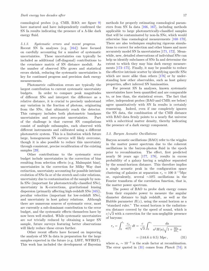
5.2. Baryon Acoustic Oscillations
Baryon acoustic oscillations (BAO) refer to the wigglesin the matter power spectrum due to the coherentoscillations in the baryon-photon fluid in the epochprior to recombination. The effect, first predictednearly 50 years ago [177, 178], results in excessprobability of a galaxy having a neighbor separatedby the sound-horizon distance. This therefore impliesa single acoustic peak in the configuration spaceclustering of galaxies at separation rs ' 100 h−1Mpcor, equivalently, several ∼10% oscillations in theFourier transform of the correlation function, that is,the matter power spectrum.
The power of BAO to probe dark energy comesfrom their exquisite power to measure the angulardiameter distance to high redshift, as well as theHubble parameter H(z), using the sound horizon as a“standard ruler.” The sound horizon is the radiation-era distance covered by the speed of sound, which isc/√
3 with a correction for the non-negligible presenceof baryons:
rs =
∫ t∗
0
csa(t)
dt =c√3
∫ a∗
0
da
a2H(a)√
1 + 3Ωb4Ωγ
a
= (144.6± 0.5) Mpc , (31)
where a∗ ∼ 10−3 is the scale factor at recombination.The error quoted in (31) comes from Planck [74]; it
Dark energy two decades after 18
is known independently to such a high precision dueto measurements of the physical matter and baryondensities from the morphology of the peaks in the CMBangular power spectrum.
A pioneering detection of the BAO feature wasmade from analysis of the Sloan Digital Sky Survey(SDSS) galaxy data [179]. Much improvement has beenmade in subsequent measurements [180–187].
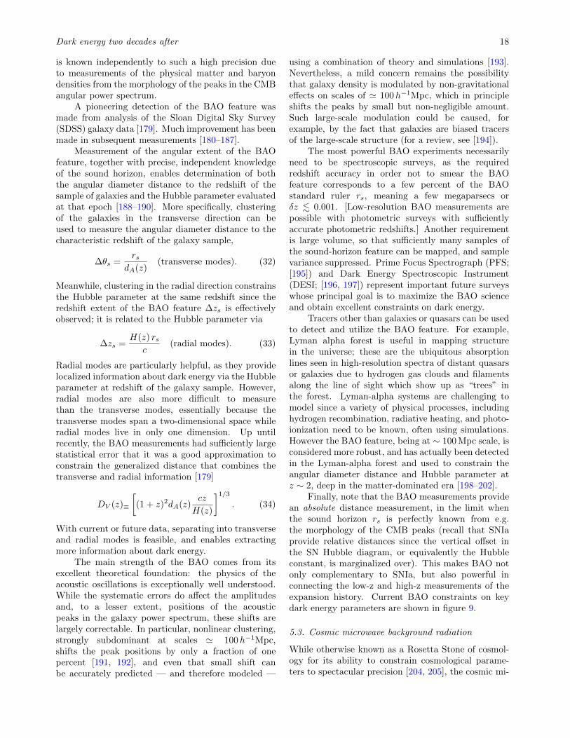
Measurement of the angular extent of the BAOfeature, together with precise, independent knowledgeof the sound horizon, enables determination of boththe angular diameter distance to the redshift of thesample of galaxies and the Hubble parameter evaluatedat that epoch [188–190]. More specifically, clusteringof the galaxies in the transverse direction can beused to measure the angular diameter distance to thecharacteristic redshift of the galaxy sample,
∆θs =rs
dA(z)(transverse modes). (32)
Meanwhile, clustering in the radial direction constrainsthe Hubble parameter at the same redshift since theredshift extent of the BAO feature ∆zs is effectivelyobserved; it is related to the Hubble parameter via
∆zs =H(z) rs
c(radial modes). (33)
Radial modes are particularly helpful, as they providelocalized information about dark energy via the Hubbleparameter at redshift of the galaxy sample. However,radial modes are also more difficult to measurethan the transverse modes, essentially because thetransverse modes span a two-dimensional space whileradial modes live in only one dimension. Up untilrecently, the BAO measurements had sufficiently largestatistical error that it was a good approximation toconstrain the generalized distance that combines thetransverse and radial information [179]
DV (z)≡
[(1 + z)2dA(z)
cz
H(z)
]1/3
. (34)
With current or future data, separating into transverseand radial modes is feasible, and enables extractingmore information about dark energy.
The main strength of the BAO comes from itsexcellent theoretical foundation: the physics of theacoustic oscillations is exceptionally well understood.While the systematic errors do affect the amplitudesand, to a lesser extent, positions of the acousticpeaks in the galaxy power spectrum, these shifts arelargely correctable. In particular, nonlinear clustering,strongly subdominant at scales ' 100h−1Mpc,shifts the peak positions by only a fraction of onepercent [191, 192], and even that small shift canbe accurately predicted — and therefore modeled —
using a combination of theory and simulations [193].Nevertheless, a mild concern remains the possibilitythat galaxy density is modulated by non-gravitationaleffects on scales of ' 100h−1Mpc, which in principleshifts the peaks by small but non-negligible amount.Such large-scale modulation could be caused, forexample, by the fact that galaxies are biased tracersof the large-scale structure (for a review, see [194]).
The most powerful BAO experiments necessarilyneed to be spectroscopic surveys, as the requiredredshift accuracy in order not to smear the BAOfeature corresponds to a few percent of the BAOstandard ruler rs, meaning a few megaparsecs orδz . 0.001. [Low-resolution BAO measurements arepossible with photometric surveys with sufficientlyaccurate photometric redshifts.] Another requirementis large volume, so that sufficiently many samples ofthe sound-horizon feature can be mapped, and samplevariance suppressed. Prime Focus Spectrograph (PFS;[195]) and Dark Energy Spectroscopic Instrument(DESI; [196, 197]) represent important future surveyswhose principal goal is to maximize the BAO scienceand obtain excellent constraints on dark energy.
Tracers other than galaxies or quasars can be usedto detect and utilize the BAO feature. For example,Lyman alpha forest is useful in mapping structurein the universe; these are the ubiquitous absorptionlines seen in high-resolution spectra of distant quasarsor galaxies due to hydrogen gas clouds and filamentsalong the line of sight which show up as “trees” inthe forest. Lyman-alpha systems are challenging tomodel since a variety of physical processes, includinghydrogen recombination, radiative heating, and photo-ionization need to be known, often using simulations.However the BAO feature, being at ∼ 100 Mpc scale, isconsidered more robust, and has actually been detectedin the Lyman-alpha forest and used to constrain theangular diameter distance and Hubble parameter atz ∼ 2, deep in the matter-dominated era [198–202].
Finally, note that the BAO measurements providean absolute distance measurement, in the limit whenthe sound horizon rs is perfectly known from e.g.the morphology of the CMB peaks (recall that SNIaprovide relative distances since the vertical offset inthe SN Hubble diagram, or equivalently the Hubbleconstant, is marginalized over). This makes BAO notonly complementary to SNIa, but also powerful inconnecting the low-z and high-z measurements of theexpansion history. Current BAO constraints on keydark energy parameters are shown in figure 9.
5.3. Cosmic microwave background radiation
While otherwise known as a Rosetta Stone of cosmol-ogy for its ability to constrain cosmological parame-ters to spectacular precision [204, 205], the cosmic mi-
Dark energy two decades after 19
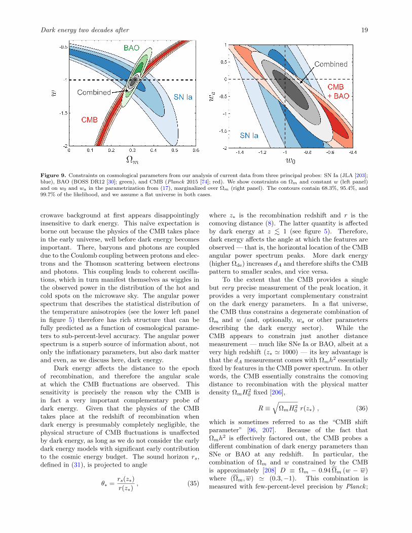
Figure 9. Constraints on cosmological parameters from our analysis of current data from three principal probes: SN Ia (JLA [203];blue), BAO (BOSS DR12 [30]; green), and CMB (Planck 2015 [74]; red). We show constraints on Ωm and constant w (left panel)and on w0 and wa in the parametrization from (17), marginalized over Ωm (right panel). The contours contain 68.3%, 95.4%, and99.7% of the likelihood, and we assume a flat universe in both cases.
crowave background at first appears disappointinglyinsensitive to dark energy. This naıve expectation isborne out because the physics of the CMB takes placein the early universe, well before dark energy becomesimportant. There, baryons and photons are coupleddue to the Coulomb coupling between protons and elec-trons and the Thomson scattering between electronsand photons. This coupling leads to coherent oscilla-tions, which in turn manifest themselves as wiggles inthe observed power in the distribution of the hot andcold spots on the microwave sky. The angular powerspectrum that describes the statistical distribution ofthe temperature anisotropies (see the lower left panelin figure 5) therefore has rich structure that can befully predicted as a function of cosmological parame-ters to sub-percent-level accuracy. The angular powerspectrum is a superb source of information about, notonly the inflationary parameters, but also dark matterand even, as we discuss here, dark energy.
Dark energy affects the distance to the epochof recombination, and therefore the angular scaleat which the CMB fluctuations are observed. Thissensitivity is precisely the reason why the CMB isin fact a very important complementary probe ofdark energy. Given that the physics of the CMBtakes place at the redshift of recombination whendark energy is presumably completely negligible, thephysical structure of CMB fluctuations is unaffectedby dark energy, as long as we do not consider the earlydark energy models with significant early contributionto the cosmic energy budget. The sound horizon rs,defined in (31), is projected to angle
θ∗ =rs(z∗)
r(z∗), (35)
where z∗ is the recombination redshift and r is thecomoving distance (8). The latter quantity is affectedby dark energy at z . 1 (see figure 5). Therefore,dark energy affects the angle at which the features areobserved — that is, the horizontal location of the CMBangular power spectrum peaks. More dark energy(higher Ωde) increases dA and therefore shifts the CMBpattern to smaller scales, and vice versa.
To the extent that the CMB provides a singlebut very precise measurement of the peak location, itprovides a very important complementary constrainton the dark energy parameters. In a flat universe,the CMB thus constrains a degenerate combination ofΩm and w (and, optionally, wa or other parametersdescribing the dark energy sector). While theCMB appears to constrain just another distancemeasurement — much like SNe Ia or BAO, albeit at avery high redshift (z∗ ' 1000) — its key advantage isthat the dA measurement comes with Ωmh
2 essentiallyfixed by features in the CMB power spectrum. In otherwords, the CMB essentially constrains the comovingdistance to recombination with the physical matterdensity ΩmH
20 fixed [206],
R ≡√
ΩmH20 r(z∗) , (36)
which is sometimes referred to as the “CMB shiftparameter” [96, 207]. Because of the fact thatΩmh
2 is effectively factored out, the CMB probes adifferent combination of dark energy parameters thanSNe or BAO at any redshift. In particular, thecombination of Ωm and w constrained by the CMBis approximately [208] D ≡ Ωm − 0.94 Ωm (w − w)where (Ωm, w) ' (0.3,−1). This combination ismeasured with few-percent-level precision by Planck ;
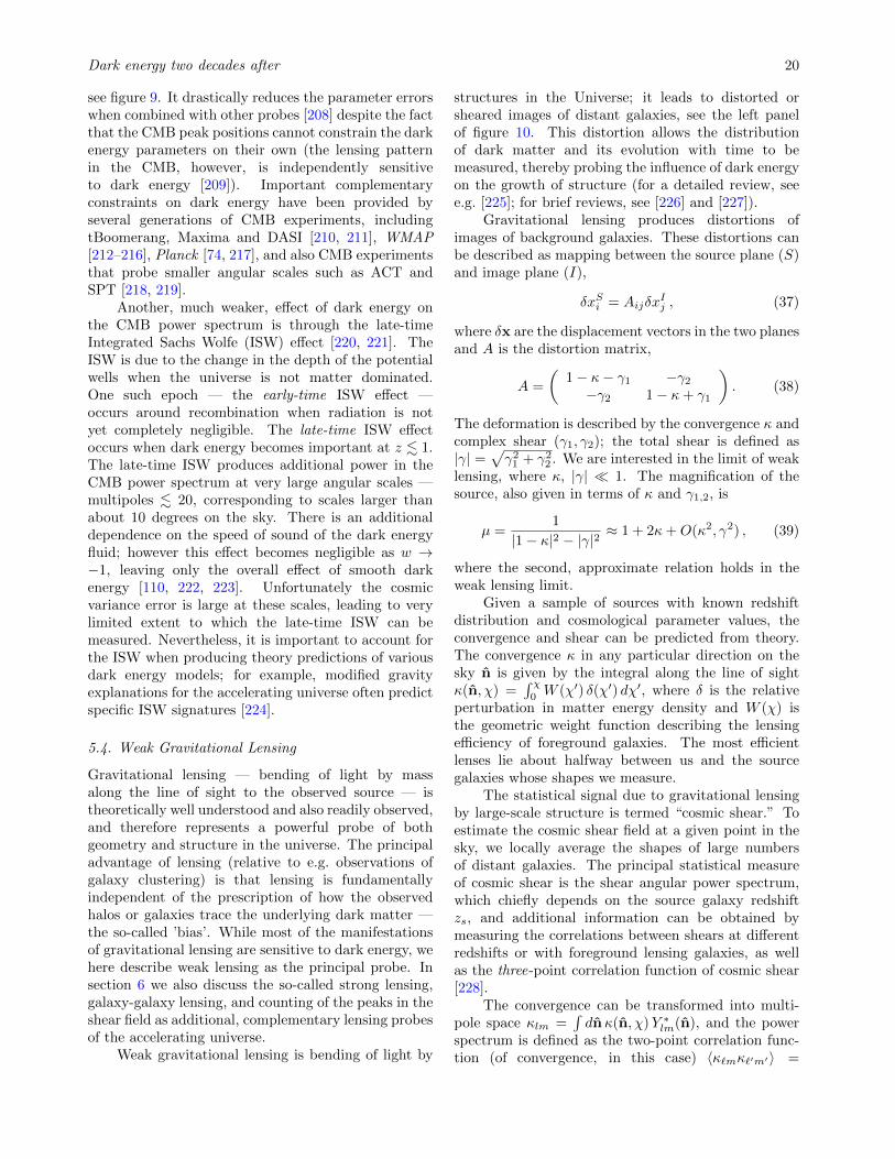
Dark energy two decades after 20
see figure 9. It drastically reduces the parameter errorswhen combined with other probes [208] despite the factthat the CMB peak positions cannot constrain the darkenergy parameters on their own (the lensing patternin the CMB, however, is independently sensitiveto dark energy [209]). Important complementaryconstraints on dark energy have been provided byseveral generations of CMB experiments, includingtBoomerang, Maxima and DASI [210, 211], WMAP[212–216], Planck [74, 217], and also CMB experimentsthat probe smaller angular scales such as ACT andSPT [218, 219].
Another, much weaker, effect of dark energy onthe CMB power spectrum is through the late-timeIntegrated Sachs Wolfe (ISW) effect [220, 221]. TheISW is due to the change in the depth of the potentialwells when the universe is not matter dominated.One such epoch — the early-time ISW effect —occurs around recombination when radiation is notyet completely negligible. The late-time ISW effectoccurs when dark energy becomes important at z . 1.The late-time ISW produces additional power in theCMB power spectrum at very large angular scales —multipoles . 20, corresponding to scales larger thanabout 10 degrees on the sky. There is an additionaldependence on the speed of sound of the dark energyfluid; however this effect becomes negligible as w →−1, leaving only the overall effect of smooth darkenergy [110, 222, 223]. Unfortunately the cosmicvariance error is large at these scales, leading to verylimited extent to which the late-time ISW can bemeasured. Nevertheless, it is important to account forthe ISW when producing theory predictions of variousdark energy models; for example, modified gravityexplanations for the accelerating universe often predictspecific ISW signatures [224].
5.4. Weak Gravitational Lensing
Gravitational lensing — bending of light by massalong the line of sight to the observed source — istheoretically well understood and also readily observed,and therefore represents a powerful probe of bothgeometry and structure in the universe. The principaladvantage of lensing (relative to e.g. observations ofgalaxy clustering) is that lensing is fundamentallyindependent of the prescription of how the observedhalos or galaxies trace the underlying dark matter —the so-called ’bias’. While most of the manifestationsof gravitational lensing are sensitive to dark energy, wehere describe weak lensing as the principal probe. Insection 6 we also discuss the so-called strong lensing,galaxy-galaxy lensing, and counting of the peaks in theshear field as additional, complementary lensing probesof the accelerating universe.
Weak gravitational lensing is bending of light by
structures in the Universe; it leads to distorted orsheared images of distant galaxies, see the left panelof figure 10. This distortion allows the distributionof dark matter and its evolution with time to bemeasured, thereby probing the influence of dark energyon the growth of structure (for a detailed review, seee.g. [225]; for brief reviews, see [226] and [227]).
Gravitational lensing produces distortions ofimages of background galaxies. These distortions canbe described as mapping between the source plane (S)and image plane (I),
δxSi = AijδxIj , (37)
where δx are the displacement vectors in the two planesand A is the distortion matrix,
A =
(1− κ− γ1 −γ2
−γ2 1− κ+ γ1
). (38)
The deformation is described by the convergence κ andcomplex shear (γ1, γ2); the total shear is defined as|γ| =
√γ2
1 + γ22 . We are interested in the limit of weak
lensing, where κ, |γ| 1. The magnification of thesource, also given in terms of κ and γ1,2, is
µ =1
|1− κ|2 − |γ|2≈ 1 + 2κ+O(κ2, γ2) , (39)
where the second, approximate relation holds in theweak lensing limit.
Given a sample of sources with known redshiftdistribution and cosmological parameter values, theconvergence and shear can be predicted from theory.The convergence κ in any particular direction on thesky n is given by the integral along the line of sightκ(n, χ) =
∫ χ0W (χ′) δ(χ′) dχ′, where δ is the relative
perturbation in matter energy density and W (χ) isthe geometric weight function describing the lensingefficiency of foreground galaxies. The most efficientlenses lie about halfway between us and the sourcegalaxies whose shapes we measure.
The statistical signal due to gravitational lensingby large-scale structure is termed “cosmic shear.” Toestimate the cosmic shear field at a given point in thesky, we locally average the shapes of large numbersof distant galaxies. The principal statistical measureof cosmic shear is the shear angular power spectrum,which chiefly depends on the source galaxy redshiftzs, and additional information can be obtained bymeasuring the correlations between shears at differentredshifts or with foreground lensing galaxies, as wellas the three-point correlation function of cosmic shear[228].
The convergence can be transformed into multi-pole space κlm =
∫dnκ(n, χ)Y ∗lm(n), and the power
spectrum is defined as the two-point correlation func-tion (of convergence, in this case) 〈κ`mκ`′m′〉 =
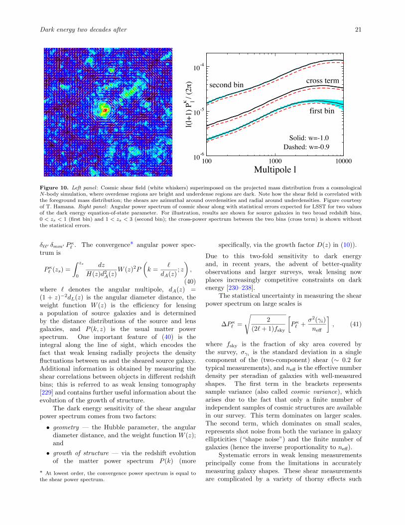
Dark energy two decades after 21
100 1000 10000Multipole l
10-6
10-5
10-4
l(l+1
) P! l /
(2")
first bin
second bin
Solid: w=-1.0Dashed: w=-0.9
cross term
Figure 10. Left panel : Cosmic shear field (white whiskers) superimposed on the projected mass distribution from a cosmologicalN -body simulation, where overdense regions are bright and underdense regions are dark. Note how the shear field is correlated withthe foreground mass distribution; the shears are azimuthal around overdensities and radial around underdensities. Figure courtesyof T. Hamana. Right panel : Angular power spectrum of cosmic shear along with statistical errors expected for LSST for two valuesof the dark energy equation-of-state parameter. For illustration, results are shown for source galaxies in two broad redshift bins,0 < zs < 1 (first bin) and 1 < zs < 3 (second bin); the cross-power spectrum between the two bins (cross term) is shown withoutthe statistical errors.
δ``′ δmm′ Pκ` . The convergence∗ angular power spec-
trum is
Pκ` (zs) =
∫ zs
0
dz
H(z)d2A(z)
W (z)2P
(k =
`
dA(z); z
),
(40)where ` denotes the angular multipole, dA(z) =(1 + z)−2dL(z) is the angular diameter distance, theweight function W (z) is the efficiency for lensinga population of source galaxies and is determinedby the distance distributions of the source and lensgalaxies, and P (k, z) is the usual matter powerspectrum. One important feature of (40) is theintegral along the line of sight, which encodes thefact that weak lensing radially projects the densityfluctuations between us and the sheared source galaxy.Additional information is obtained by measuring theshear correlations between objects in different redshiftbins; this is referred to as weak lensing tomography[229] and contains further useful information about theevolution of the growth of structure.
The dark energy sensitivity of the shear angularpower spectrum comes from two factors:
• geometry — the Hubble parameter, the angulardiameter distance, and the weight function W (z);and
• growth of structure — via the redshift evolutionof the matter power spectrum P (k) (more
∗ At lowest order, the convergence power spectrum is equal tothe shear power spectrum.
specifically, via the growth factor D(z) in (10)).
Due to this two-fold sensitivity to dark energyand, in recent years, the advent of better-qualityobservations and larger surveys, weak lensing nowplaces increasingly competitive constraints on darkenergy [230–238].
The statistical uncertainty in measuring the shearpower spectrum on large scales is
∆Pκ` =
√2
(2`+ 1)fsky
[Pκ` +
σ2(γi)
neff
], (41)
where fsky is the fraction of sky area covered bythe survey, σγi is the standard deviation in a singlecomponent of the (two-component) shear (∼ 0.2 fortypical measurements), and neff is the effective numberdensity per steradian of galaxies with well-measuredshapes. The first term in the brackets representssample variance (also called cosmic variance), whicharises due to the fact that only a finite number ofindependent samples of cosmic structures are availablein our survey. This term dominates on larger scales.The second term, which dominates on small scales,represents shot noise from both the variance in galaxyellipticities (“shape noise”) and the finite number ofgalaxies (hence the inverse proportionality to neff).
Systematic errors in weak lensing measurementsprincipally come from the limitations in accuratelymeasuring galaxy shapes. These shear measurementsare complicated by a variety of thorny effects such

Dark energy two decades after 22
as the atmospheric blurring of the images, telescopedistortions, charge transfer in CCDs, to name just afew. More generally, a given measurement of the galaxyshear will be subject to additive and multiplicativeerrors that affect the true shear [239, 240]. Theweak lensing community has embarked on a series ofchallenges to develop algorithms and techniques toameliorate these observational systematics (e.g. [241]).There are also systematic uncertainties due to limitedknowledge of the redshifts of source galaxies: becausetaking spectroscopic redshifts of most source galaxieswill be impossible (for upcoming surveys, that numberwill be of order a billion), the community has developedapproximate photometric redshift techniques, whereone obtains a noisy redshift estimate from multi-wavelength (i.e. multi-color) observations of eachgalaxy. In order for the photometric redshift biases notto degrade future dark energy constraints, their meancalibration at the 0.1% level will be required [242, 243].
The interpretation of weak lensing measurementsalso faces theoretical challenges, such as the needto have accurate predictions for clustering in thenon-linear regime from N-body simulations [244–246]and to account for non-Gaussian errors on smallangular scales [247–249]. Finally, intrinsic alignmentsof galaxy shapes, due to tidal gravitational fields,are a serious contaminant which requires carefulmodeling as well as external astrophysics input, such asobservationally-inferred galaxy separation, type, andluminosity information; for a review, see [250].
The right panel of figure 10 shows the weak lensingshear power spectrum for two values of w, and thecorresponding statistical errors expected for a surveysuch as LSST, assuming a survey area of 15,000 deg2
and effective source galaxy density of neff = 30 galaxiesper square arcminute, and divided into two radialslices. Current surveys cover more modest hundredsof deg2, although KIDS (450, and soon to be up to1,500 deg2 [237]), Dark Energy Survey (about 1,500and soon to be 5,000 deg2 [251]) and Hyper Suprime-Cam (HSC; expected to be 1,500 deg2 [252]) are aimingto bring weak lensing to the forefront of dark energyconstraints. Note that the proportionality of errors
to f−1/2sky means that, as long as the systematic errors
can be controlled, large sky coverage is at a premium.Further improvement in dark energy constraints can beachieved by judiciously combining a photometric anda spectroscopic survey [253–258].
The weak lensing signal can also be used todetect and count massive halos, particularly galaxyclusters. This method, pioneered recently [259,260], can be used to obtain cluster samples whosemasses are reliably determined, avoiding the arguablymore difficult signal-to-mass conversions required withthe X-ray or optical observations [261–264]. Much
important information about the dark matter andgas content of galaxy clusters can be inferred withthe combined lensing, X-ray, and optical observations.This has recently been demonstrated with observationsof the “Bullet Cluster” [265], where the dark matterdistribution inferred from weak lensing is clearly offsetfrom the hot gas inferred from the X-ray observations,indicating the presence and distinctive fingerprints ofdark matter.
5.5. Galaxy clusters
Galaxy clusters — the largest collapsed objects in theuniverse with mass & 1014M and size a few Mpc –are just simple enough that their spatial abundanceand internal structure can be used to probe darkenergy. Clusters are versatile probes of cosmology andastrophysics and have had an important role in thedevelopment of modern cosmology (for a review, see[266]). In the context of dark energy, one can usethe spatial abundance of clusters and compare it tothe theoretical expectation that includes the effectsof dark energy. This classic test is in principle verysimple, since the number density of clusters can beinferred from purely theoretical considerations or, morerobustly, from suites of numerical simulations. Inpractice, however, there are important challenges toovercome.
The number of halos in the mass range [M,M +dM ] in a patch of the sky with solid angle dΩ and inredshift interval [z, z + dz] is given by
d2N
dΩdz=r2(z)
H(z)
dn(M, z)
dMdM , (42)
where r2/H = dV/(dΩdz) is the comoving volumeelement and n(M, z) is the number density (the“mass function”) that is calibrated with numericalsimulations (e.g. [267]).
Assuming Gaussian initial conditions, the comov-ing number density of objects in an interval dM aroundmass M is
dn
d lnM=ρM,0
M
∣∣∣∣dF (M)
d lnM
∣∣∣∣ , (43)
where ρM,0 is evaluated at the present time andF (M) is the fraction of collapsed objects. Theoriginal analysis of Press and Schechter [268] assumed aGaussian initial distribution of overdensities, leading toF (M) = (1/2) erfc(ν/
√2), where ν(M) ≡ δc/σ(M) is
the peak height and δc = 1.686 is the critical thresholdfor collapse in the spherical top-hat model [269]. ThePress-Schechter formula also involves multiplying themass function by the notorious overall factor of twoto account for underdensities as well as overdensities.Subsequent work has put the theoretical estimates on
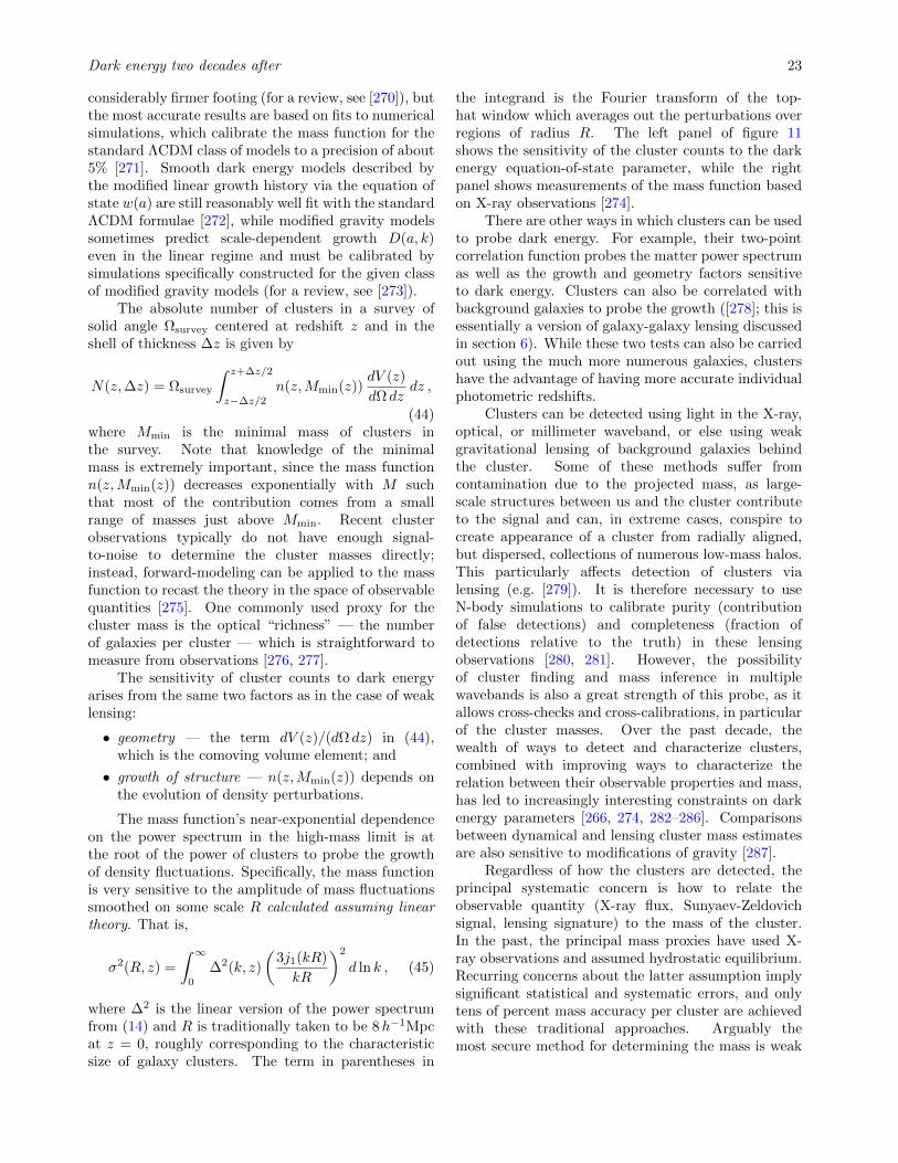
Dark energy two decades after 23
considerably firmer footing (for a review, see [270]), butthe most accurate results are based on fits to numericalsimulations, which calibrate the mass function for thestandard ΛCDM class of models to a precision of about5% [271]. Smooth dark energy models described bythe modified linear growth history via the equation ofstate w(a) are still reasonably well fit with the standardΛCDM formulae [272], while modified gravity modelssometimes predict scale-dependent growth D(a, k)even in the linear regime and must be calibrated bysimulations specifically constructed for the given classof modified gravity models (for a review, see [273]).
The absolute number of clusters in a survey ofsolid angle Ωsurvey centered at redshift z and in theshell of thickness ∆z is given by
N(z,∆z) = Ωsurvey
∫ z+∆z/2
z−∆z/2
n(z,Mmin(z))dV (z)
dΩ dzdz ,
(44)where Mmin is the minimal mass of clusters inthe survey. Note that knowledge of the minimalmass is extremely important, since the mass functionn(z,Mmin(z)) decreases exponentially with M suchthat most of the contribution comes from a smallrange of masses just above Mmin. Recent clusterobservations typically do not have enough signal-to-noise to determine the cluster masses directly;instead, forward-modeling can be applied to the massfunction to recast the theory in the space of observablequantities [275]. One commonly used proxy for thecluster mass is the optical “richness” — the numberof galaxies per cluster — which is straightforward tomeasure from observations [276, 277].
The sensitivity of cluster counts to dark energyarises from the same two factors as in the case of weaklensing:
• geometry — the term dV (z)/(dΩ dz) in (44),which is the comoving volume element; and
• growth of structure — n(z,Mmin(z)) depends onthe evolution of density perturbations.
The mass function’s near-exponential dependenceon the power spectrum in the high-mass limit is atthe root of the power of clusters to probe the growthof density fluctuations. Specifically, the mass functionis very sensitive to the amplitude of mass fluctuationssmoothed on some scale R calculated assuming lineartheory. That is,
σ2(R, z) =
∫ ∞0
∆2(k, z)
(3j1(kR)
kR
)2
d ln k , (45)
where ∆2 is the linear version of the power spectrumfrom (14) and R is traditionally taken to be 8h−1Mpcat z = 0, roughly corresponding to the characteristicsize of galaxy clusters. The term in parentheses in
the integrand is the Fourier transform of the top-hat window which averages out the perturbations overregions of radius R. The left panel of figure 11shows the sensitivity of the cluster counts to the darkenergy equation-of-state parameter, while the rightpanel shows measurements of the mass function basedon X-ray observations [274].
There are other ways in which clusters can be usedto probe dark energy. For example, their two-pointcorrelation function probes the matter power spectrumas well as the growth and geometry factors sensitiveto dark energy. Clusters can also be correlated withbackground galaxies to probe the growth ([278]; this isessentially a version of galaxy-galaxy lensing discussedin section 6). While these two tests can also be carriedout using the much more numerous galaxies, clustershave the advantage of having more accurate individualphotometric redshifts.
Clusters can be detected using light in the X-ray,optical, or millimeter waveband, or else using weakgravitational lensing of background galaxies behindthe cluster. Some of these methods suffer fromcontamination due to the projected mass, as large-scale structures between us and the cluster contributeto the signal and can, in extreme cases, conspire tocreate appearance of a cluster from radially aligned,but dispersed, collections of numerous low-mass halos.This particularly affects detection of clusters vialensing (e.g. [279]). It is therefore necessary to useN-body simulations to calibrate purity (contributionof false detections) and completeness (fraction ofdetections relative to the truth) in these lensingobservations [280, 281]. However, the possibilityof cluster finding and mass inference in multiplewavebands is also a great strength of this probe, as itallows cross-checks and cross-calibrations, in particularof the cluster masses. Over the past decade, thewealth of ways to detect and characterize clusters,combined with improving ways to characterize therelation between their observable properties and mass,has led to increasingly interesting constraints on darkenergy parameters [266, 274, 282–286]. Comparisonsbetween dynamical and lensing cluster mass estimatesare also sensitive to modifications of gravity [287].
Regardless of how the clusters are detected, theprincipal systematic concern is how to relate theobservable quantity (X-ray flux, Sunyaev-Zeldovichsignal, lensing signature) to the mass of the cluster.In the past, the principal mass proxies have used X-ray observations and assumed hydrostatic equilibrium.Recurring concerns about the latter assumption implysignificant statistical and systematic errors, and onlytens of percent mass accuracy per cluster are achievedwith these traditional approaches. Arguably themost secure method for determining the mass is weak
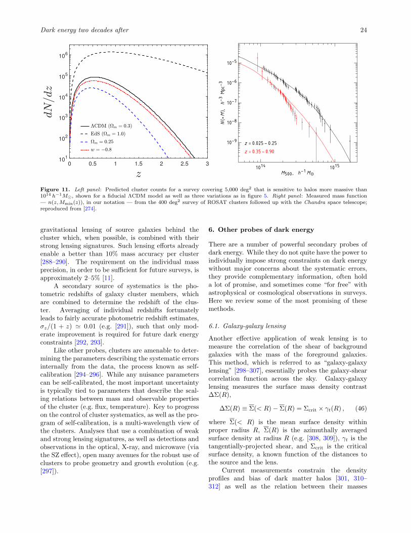
Dark energy two decades after 24
0 0.5 1 1.5 2 2.5 310
1
102
103
104
105
106
z = 0.025 − 0.25
1014 1015
10−9
10−8
10−7
10−6
10−5
M500, h−1
M⊙
N(>
M),
h−
3Mpc−
3
z = 0.35 − 0.90
Figure 11. Left panel : Predicted cluster counts for a survey covering 5,000 deg2 that is sensitive to halos more massive than1014 h−1M, shown for a fiducial ΛCDM model as well as three variations as in figure 5. Right panel : Measured mass function— n(z,Mmin(z)), in our notation — from the 400 deg2 survey of ROSAT clusters followed up with the Chandra space telescope;reproduced from [274].
gravitational lensing of source galaxies behind thecluster which, when possible, is combined with theirstrong lensing signatures. Such lensing efforts alreadyenable a better than 10% mass accuracy per cluster[288–290]. The requirement on the individual massprecision, in order to be sufficient for future surveys, isapproximately 2–5% [11].
A secondary source of systematics is the pho-tometric redshifts of galaxy cluster members, whichare combined to determine the redshift of the clus-ter. Averaging of individual redshifts fortunatelyleads to fairly accurate photometric redshift estimates,σz/(1 + z) ' 0.01 (e.g. [291]), such that only mod-erate improvement is required for future dark energyconstraints [292, 293].
Like other probes, clusters are amenable to deter-mining the parameters describing the systematic errorsinternally from the data, the process known as self-calibration [294–296]. While any nuisance parameterscan be self-calibrated, the most important uncertaintyis typically tied to parameters that describe the scal-ing relations between mass and observable propertiesof the cluster (e.g. flux, temperature). Key to progresson the control of cluster systematics, as well as the pro-gram of self-calibration, is a multi-wavelength view ofthe clusters. Analyses that use a combination of weakand strong lensing signatures, as well as detections andobservations in the optical, X-ray, and microwave (viathe SZ effect), open many avenues for the robust use ofclusters to probe geometry and growth evolution (e.g.[297]).
6. Other probes of dark energy
There are a number of powerful secondary probes ofdark energy. While they do not quite have the power toindividually impose strong constraints on dark energywithout major concerns about the systematic errors,they provide complementary information, often holda lot of promise, and sometimes come “for free” withastrophysical or cosmological observations in surveys.Here we review some of the most promising of thesemethods.
6.1. Galaxy-galaxy lensing
Another effective application of weak lensing is tomeasure the correlation of the shear of backgroundgalaxies with the mass of the foreground galaxies.This method, which is referred to as “galaxy-galaxylensing” [298–307], essentially probes the galaxy-shearcorrelation function across the sky. Galaxy-galaxylensing measures the surface mass density contrast∆Σ(R),
∆Σ(R) ≡ Σ(< R)− Σ(R) = Σcrit × γt(R) , (46)
where Σ(< R) is the mean surface density withinproper radius R, Σ(R) is the azimuthally averagedsurface density at radius R (e.g. [308, 309]), γt is thetangentially-projected shear, and Σcrit is the criticalsurface density, a known function of the distances tothe source and the lens.
Current measurements constrain the densityprofiles and bias of dark matter halos [301, 310–312] as well as the relation between their masses
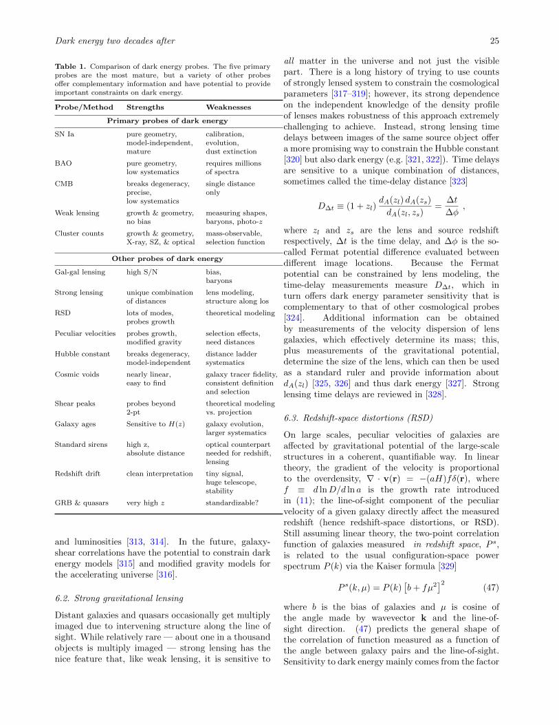
Dark energy two decades after 25
Table 1. Comparison of dark energy probes. The five primaryprobes are the most mature, but a variety of other probesoffer complementary information and have potential to provideimportant constraints on dark energy.
Probe/Method Strengths Weaknesses
Primary probes of dark energy
SN Ia pure geometry, calibration,model-independent, evolution,mature dust extinction
BAO pure geometry, requires millionslow systematics of spectra
CMB breaks degeneracy, single distanceprecise, onlylow systematics
Weak lensing growth & geometry, measuring shapes,no bias baryons, photo-z
Cluster counts growth & geometry, mass-observable,X-ray, SZ, & optical selection function
Other probes of dark energy
Gal-gal lensing high S/N bias,baryons
Strong lensing unique combination lens modeling,of distances structure along los
RSD lots of modes, theoretical modelingprobes growth
Peculiar velocities probes growth, selection effects,modified gravity need distances
Hubble constant breaks degeneracy, distance laddermodel-independent systematics
Cosmic voids nearly linear, galaxy tracer fidelity,easy to find consistent definition
and selection
Shear peaks probes beyond theoretical modeling2-pt vs. projection
Galaxy ages Sensitive to H(z) galaxy evolution,larger systematics
Standard sirens high z, optical counterpartabsolute distance needed for redshift,
lensing
Redshift drift clean interpretation tiny signal,huge telescope,stability
GRB & quasars very high z standardizable?
and luminosities [313, 314]. In the future, galaxy-shear correlations have the potential to constrain darkenergy models [315] and modified gravity models forthe accelerating universe [316].
6.2. Strong gravitational lensing
Distant galaxies and quasars occasionally get multiplyimaged due to intervening structure along the line ofsight. While relatively rare — about one in a thousandobjects is multiply imaged — strong lensing has thenice feature that, like weak lensing, it is sensitive to
all matter in the universe and not just the visiblepart. There is a long history of trying to use countsof strongly lensed system to constrain the cosmologicalparameters [317–319]; however, its strong dependenceon the independent knowledge of the density profileof lenses makes robustness of this approach extremelychallenging to achieve. Instead, strong lensing timedelays between images of the same source object offera more promising way to constrain the Hubble constant[320] but also dark energy (e.g. [321, 322]). Time delaysare sensitive to a unique combination of distances,sometimes called the time-delay distance [323]
D∆t ≡ (1 + zl)dA(zl) dA(zs)
dA(zl, zs)=
∆t
∆φ,
where zl and zs are the lens and source redshiftrespectively, ∆t is the time delay, and ∆φ is the so-called Fermat potential difference evaluated betweendifferent image locations. Because the Fermatpotential can be constrained by lens modeling, thetime-delay measurements measure D∆t, which inturn offers dark energy parameter sensitivity that iscomplementary to that of other cosmological probes[324]. Additional information can be obtainedby measurements of the velocity dispersion of lensgalaxies, which effectively determine its mass; this,plus measurements of the gravitational potential,determine the size of the lens, which can then be usedas a standard ruler and provide information aboutdA(zl) [325, 326] and thus dark energy [327]. Stronglensing time delays are reviewed in [328].
6.3. Redshift-space distortions (RSD)
On large scales, peculiar velocities of galaxies areaffected by gravitational potential of the large-scalestructures in a coherent, quantifiable way. In lineartheory, the gradient of the velocity is proportionalto the overdensity, ∇ · v(r) = −(aH)fδ(r), wheref ≡ d lnD/d ln a is the growth rate introducedin (11); the line-of-sight component of the peculiarvelocity of a given galaxy directly affect the measuredredshift (hence redshift-space distortions, or RSD).Still assuming linear theory, the two-point correlationfunction of galaxies measured in redshift space, P s,is related to the usual configuration-space powerspectrum P (k) via the Kaiser formula [329]
P s(k, µ) = P (k)[b+ fµ2
]2(47)
where b is the bias of galaxies and µ is cosine ofthe angle made by wavevector k and the line-of-sight direction. (47) predicts the general shape ofthe correlation of function measured as a function ofthe angle between galaxy pairs and the line-of-sight.Sensitivity to dark energy mainly comes from the factor
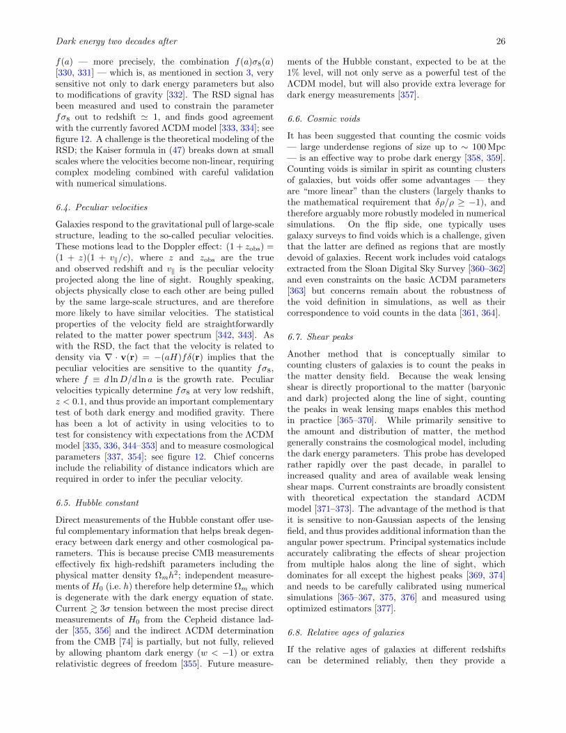
Dark energy two decades after 26
f(a) — more precisely, the combination f(a)σ8(a)[330, 331] — which is, as mentioned in section 3, verysensitive not only to dark energy parameters but alsoto modifications of gravity [332]. The RSD signal hasbeen measured and used to constrain the parameterfσ8 out to redshift ' 1, and finds good agreementwith the currently favored ΛCDM model [333, 334]; seefigure 12. A challenge is the theoretical modeling of theRSD; the Kaiser formula in (47) breaks down at smallscales where the velocities become non-linear, requiringcomplex modeling combined with careful validationwith numerical simulations.
6.4. Peculiar velocities
Galaxies respond to the gravitational pull of large-scalestructure, leading to the so-called peculiar velocities.These motions lead to the Doppler effect: (1 + zobs) =(1 + z)(1 + v‖/c), where z and zobs are the trueand observed redshift and v‖ is the peculiar velocityprojected along the line of sight. Roughly speaking,objects physically close to each other are being pulledby the same large-scale structures, and are thereforemore likely to have similar velocities. The statisticalproperties of the velocity field are straightforwardlyrelated to the matter power spectrum [342, 343]. Aswith the RSD, the fact that the velocity is related todensity via ∇ · v(r) = −(aH)fδ(r) implies that thepeculiar velocities are sensitive to the quantity fσ8,where f ≡ d lnD/d ln a is the growth rate. Peculiarvelocities typically determine fσ8 at very low redshift,z < 0.1, and thus provide an important complementarytest of both dark energy and modified gravity. Therehas been a lot of activity in using velocities to totest for consistency with expectations from the ΛCDMmodel [335, 336, 344–353] and to measure cosmologicalparameters [337, 354]; see figure 12. Chief concernsinclude the reliability of distance indicators which arerequired in order to infer the peculiar velocity.
6.5. Hubble constant
Direct measurements of the Hubble constant offer use-ful complementary information that helps break degen-eracy between dark energy and other cosmological pa-rameters. This is because precise CMB measurementseffectively fix high-redshift parameters including thephysical matter density Ωmh
2; independent measure-ments of H0 (i.e. h) therefore help determine Ωm whichis degenerate with the dark energy equation of state.Current & 3σ tension between the most precise directmeasurements of H0 from the Cepheid distance lad-der [355, 356] and the indirect ΛCDM determinationfrom the CMB [74] is partially, but not fully, relievedby allowing phantom dark energy (w < −1) or extrarelativistic degrees of freedom [355]. Future measure-
ments of the Hubble constant, expected to be at the1% level, will not only serve as a powerful test of theΛCDM model, but will also provide extra leverage fordark energy measurements [357].
6.6. Cosmic voids
It has been suggested that counting the cosmic voids— large underdense regions of size up to ∼ 100 Mpc— is an effective way to probe dark energy [358, 359].Counting voids is similar in spirit as counting clustersof galaxies, but voids offer some advantages — theyare “more linear” than the clusters (largely thanks tothe mathematical requirement that δρ/ρ ≥ −1), andtherefore arguably more robustly modeled in numericalsimulations. On the flip side, one typically usesgalaxy surveys to find voids which is a challenge, giventhat the latter are defined as regions that are mostlydevoid of galaxies. Recent work includes void catalogsextracted from the Sloan Digital Sky Survey [360–362]and even constraints on the basic ΛCDM parameters[363] but concerns remain about the robustness ofthe void definition in simulations, as well as theircorrespondence to void counts in the data [361, 364].
6.7. Shear peaks
Another method that is conceptually similar tocounting clusters of galaxies is to count the peaks inthe matter density field. Because the weak lensingshear is directly proportional to the matter (baryonicand dark) projected along the line of sight, countingthe peaks in weak lensing maps enables this methodin practice [365–370]. While primarily sensitive tothe amount and distribution of matter, the methodgenerally constrains the cosmological model, includingthe dark energy parameters. This probe has developedrather rapidly over the past decade, in parallel toincreased quality and area of available weak lensingshear maps. Current constraints are broadly consistentwith theoretical expectation the standard ΛCDMmodel [371–373]. The advantage of the method is thatit is sensitive to non-Gaussian aspects of the lensingfield, and thus provides additional information than theangular power spectrum. Principal systematics includeaccurately calibrating the effects of shear projectionfrom multiple halos along the line of sight, whichdominates for all except the highest peaks [369, 374]and needs to be carefully calibrated using numericalsimulations [365–367, 375, 376] and measured usingoptimized estimators [377].
6.8. Relative ages of galaxies
If the relative ages of galaxies at different redshiftscan be determined reliably, then they provide a
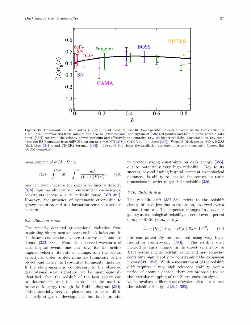
Dark energy two decades after 27
0 0.2 0.4 0.6 0.8z
0
0.1
0.2
0.3
0.4
0.5
0.6
f(z)σ8(z)
6dF+
6dF
GAMA
Wigglez BOSSVIPERS
SN
SN
Figure 12. Constraints on the quantity fσ8 at different redshifts from RSD and peculiar velocity surveys. At the lowest redshiftsz ≈ 0, peculiar velocities from galaxies and SNe Ia (leftmost [335] and rightmost [336] red points) and SNe Ia alone (purple datapoint; [337]) constrain the velocity power spectrum and effectively the quantity fσ8. At higher redshifts, constraints on fσ8 comefrom the RSD analyses from 6dFGS (maroon at z = 0.067; [338]), GAMA (pink points; [339]), WiggleZ (dark green; [340]), BOSS(dark blue; [341]), and VIPERS (orange; [333]). The solid line shows the prediction corresponding to the currently favored flatΛCDM cosmology.
measurement of dt/dz. Since
t(z) =
∫ t(z)
0
dt′ =
∫ ∞z
dz′
(1 + z′)H(z′), (48)
one can then measure the expansion history directly[378]. Age has already been employed in cosmologicalconstraints across a wide redshift range [379–381].However, the presence of systematic errors due togalaxy evolution and star formation remains a seriousconcern.
6.9. Standard sirens
The recently detected gravitational radiation frominspiraling binary neutron stars or black holes can, inthe future, enable these sources to serve as “standardsirens” [382, 383]. From the observed waveform ofeach inspiral event, one can solve for the orbit’sangular velocity, its rate of change, and the orbitalvelocity, in order to determine the luminosity of theobject and hence its (absolute) luminosity distance.If the electromagnetic counterpart to the observedgravitational wave signature can be unambiguouslyidentified, then the redshift of the host galaxy canbe determined, and the inspiral can be used toprobe dark energy through the Hubble diagram [384].This potentially very complementary probe is still inthe early stages of development, but holds promise
to provide strong constraints on dark energy [385],out to potentially very high redshifts. Key to itssuccess, beyond finding inspiral events at cosmologicaldistances, is ability to localize the sources in threedimensions in order to get their redshifts [386].
6.10. Redshift drift
The redshift drift [387–389] refers to the redshiftchange of an object due to expansion, observed over ahuman timescale. The expected change of a quasar orgalaxy at cosmological redshift, observed over a periodof dt0 ∼ 10–20 years, is tiny,
dz = [H0(1 + z)−H(z)] dt0 ∼ 10−9, (49)
but can potentially be measured using very high-resolution spectroscopy [390]. The redshift driftmethod is fairly unique in its direct sensitivity toH(z) across a wide redshift range and may somedaycontribute significantly to constraining the expansionhistory [391–393]. While a measurement of the redshiftdrift requires a very high telescope stability over aperiod of about a decade, there are proposals to usethe intensity mapping of the 21 cm emission signal —which involves a different set of systematics — to detectthe redshift-drift signal [394, 395].
Dark energy two decades after 28
6.11. Other standard candles/rulers
A wide variety of astronomical objects have beenproposed as standardizable candles or rulers, usefulfor inferring cosmological distances via semi-empiricalrelations. Notable examples include radio galaxiesas standardizable rulers [396, 397] and quasars asstandardizable candles, most recently via the non-linear relation between UV and X-ray luminosities[398]. Long-duration gamma-ray bursts (GRBs) arean attractive possibility [399] because their abilityto be detected at very high redshifts (z ∼ 6 orhigher) means they would probe a redshift rangebeyond that of SNe Ia. Several different relationshipsfor GRBs have been proposed, most famously theAmati relation [400, 401] between the peak energy ofthe integrated spectrum and the isotropic-equivalenttotal energy output of the GRB. Some analyses haveemployed several of these relations simultaneously[402]. Due to the relatively small number of (useful)GRBs and the substantial scatter about the relations,as well as concerns about the presence of serioussystematic errors, GRBs have not yielded competitivecosmological constraints. It remains to be seen whetherthe aforementioned relations hold over such largespans of cosmological time and can be calibrated andunderstood to a sufficient accuracy.
6.12. Observation of unexpected features
When interpreted in the context of a cosmologicalmodel (e.g. LCDM), observation of unexpectedfeatures in cosmological observations or existence ofobjects at high statistical significance can be usedto rule out the model in question. High-redshift,high-mass clusters of galaxies have been particularlydiscussed in this context: observation of clusters hadbeen used to disfavor the matter-only universe [28]while, more recently, there has been a discussion ofwhether the existence of the observed high-mass, high-redshift “pink elephant” clusters are in conflict withthe currently dominant LCDM paradigm (e.g. [403]).However such analyses requires a careful accountingof all sources of statistical error closely related tothe precise way in which the observations have beencarried out [404, 405]. Thus, while the observation ofunexpected features can be used to rule out aspectsof the dark energy paradigm, its a posteriori natureimplies that independent confirmation that uses othercosmological probes will be required.
7. The accelerating universe: Summary
In this article, we have briefly reviewed the develop-ments leading to the discovery of dark energy and theaccelerating universe. We have discussed the current
status of dark energy, described parametrizations ofthe equation of state and physical aspects that can bemeasured, and reviewed both primary and secondarycosmological probes that allow us to study this mysteri-ous component. In summary, there are a few importantthings to know about dark energy:
• Dark energy has negative pressure. It canbe described by its present-day energy densityrelative to critical Ωde and equation of statew ≡ pde/ρde. For a cosmological constant,corresponding to vacuum energy, w = −1 preciselyand at all times. More general explanations fordark energy typically lead to a time-dependentequation of state.
• Current observational data constrain the equationof state to be w ≈ −1 to within about 5%.Measuring w and any time dependence — aswell as searching for hints of any other, as yetunseen, properties of dark energy — will help usunderstand the physical nature of this mysteriouscomponent, a key goal of modern cosmology.
• Dark energy is spatially smooth. It quenches thegravitational collapse of large-scale structures andsuppresses the growth of density perturbations;whenever dark energy dominates, structures donot grow.
• Only relatively recently (z . 0.5) has darkenergy come to dominate the energy budget ofthe universe. At earlier epochs, the dark energydensity is small relative to that of matter andradiation, although a ∼1% contribution by darkenergy at early times is still allowed by the data.
• Dark energy affects both the geometry (distancesin the universe) and the growth of structure(clustering and abundance of galaxies and galaxyclusters). Separately measuring geometry andgrowth is an excellent way, not only to measuredark energy parameters, but also to differentiatebetween separate classes of dark energy models.
• Dark energy can be studied using a variety ofcosmological probes that span a wide range ofspatial and temporal scales and involve a widevariety of observable quantities. Control ofsystematic errors in these individual cosmologicalprobes is key to their ability to discriminatetestable predictions of theoretical models. Theworldwide effort in theoretically modeling andobservationally measuring dark energy reflects avibrant field with many fruitful avenues that stillremain to be explored.
REFERENCES 29
Acknowledgments
We thank Chris Blake, Gus Evrard, Eric Linder,and Fabian Schmidt for detailed comments on earlierversions of the manuscript. DH is supported by NSFgrant AST-1210974, DOE grant DEFG02-95ER40899,and NASA grant NNX16AI41G.
References
[1] Supernova Search Team Collaboration,A. G. Riess et al., Observational evidence fromsupernovae for an accelerating universe and acosmological constant, Astron. J. 116 (1998)1009–1038, [astro-ph/9805201].
[2] Supernova Cosmology ProjectCollaboration, S. Perlmutter et al.,Measurements of Omega and Lambda from 42high redshift supernovae, Astrophys. J. 517(1999) 565–586, [astro-ph/9812133].
[3] M. M. Phillips, The absolute magnitudes ofType Ia supernovae, ApJ 413 (Aug., 1993)L105–L108.
[4] A. G. Kim, The Discovery of high redshiftsupernovae and their cosmological implications.PhD thesis, UC, Berkeley, 1997.
[5] E. J. Copeland, M. Sami, and S. Tsujikawa,Dynamics of dark energy, Int. J. Mod. Phys.D15 (2006) 1753–1936, [hep-th/0603057].
[6] T. Padmanabhan, Cosmological constant: Theweight of the vacuum, Phys. Rept. 380 (2003)235–320, [hep-th/0212290].
[7] M. Li, X.-D. Li, S. Wang, and Y. Wang, DarkEnergy, Commun. Theor. Phys. 56 (2011)525–604, [arXiv:1103.5870].
[8] P. J. E. Peebles and B. Ratra, The cosmologicalconstant and dark energy, Rev. Mod. Phys. 75(2003) 559–606, [astro-ph/0207347].
[9] J.-P. Uzan, The acceleration of the universe andthe physics behind it, Gen. Rel. Grav. 39 (2007)307–342, [astro-ph/0605313].
[10] D. Huterer and M. S. Turner, Probing the darkenergy: Methods and strategies, Phys. Rev. D64(2001) 123527, [astro-ph/0012510].
[11] D. H. Weinberg, M. J. Mortonson, D. J.Eisenstein, C. Hirata, A. G. Riess, and E. Rozo,Observational Probes of Cosmic Acceleration,Phys. Rept. 530 (2013) 87–255,[arXiv:1201.2434].
[12] V. Sahni and A. Starobinsky, ReconstructingDark Energy, astro-ph/0610026 (Oct., 2006)[astro-ph/0610026].
[13] E. V. Linder, The Dynamics of Quintessence,The Quintessence of Dynamics, Gen. Rel. Grav.40 (2008) 329–356, [arXiv:0704.2064].
[14] S. M. Carroll, The cosmological constant, LivingRev. Rel. 4 (2001) 1, [astro-ph/0004075].
[15] S. Weinberg, The cosmological constantproblem, Rev. Mod. Phys. 61 (1989) 1–23.
[16] J. Frieman, M. Turner, and D. Huterer, DarkEnergy and the Accelerating Universe, Ann.Rev. Astron. Astrophys. 46 (2008) 385–432,[arXiv:0803.0982].
[17] A. H. Guth, The Inflationary Universe: APossible Solution to the Horizon and FlatnessProblems, Phys. Rev. D23 (1981) 347–356.
[18] A. D. Linde, A New Inflationary UniverseScenario: A Possible Solution of the Horizon,Flatness, Homogeneity, Isotropy and PrimordialMonopole Problems, Phys. Lett. B108 (1982)389–393.
[19] A. Albrecht and P. J. Steinhardt, Cosmology forGrand Unified Theories with RadiativelyInduced Symmetry Breaking, Phys. Rev. Lett.48 (1982) 1220–1223.
[20] A. C. Fabian, On the baryon content of theShapley Supercluster, MNRAS 253 (Dec., 1991)29P.
[21] S. D. M. White and C. S. Frenk, Galaxyformation through hierarchical clustering, ApJ379 (Sept., 1991) 52–79.
[22] S. D. M. White, J. F. Navarro, A. E. Evrard,and C. S. Frenk, The Baryon content of galaxyclusters: A Challenge to cosmological orthodoxy,Nature 366 (1993) 429–433.
[23] S. J. Maddox, G. Efstathiou, W. J. Sutherland,and J. Loveday, Galaxy correlations on largescales, Mon. Not. Roy. Astron. Soc. 242 (1990)43–49.
[24] G. Efstathiou, W. J. Sutherland, and S. J.Maddox, The cosmological constant and colddark matter, Nature 348 (1990) 705–707.
[25] Hubble Cepheid Collaboration, W. L.Freedman et al., Distance to the Virgo clustergalaxy M100 from Hubble space telescopeobservations of Cepheids, Nature 371 (1994)757–762.
[26] L. M. Krauss and B. Chaboyer, Age estimates ofglobular clusters in the milky way: Constraintson cosmology, Science 299 (2003) 65–70.
[27] M. Donahue, G. M. Voit, I. M. Gioia,G. Luppino, J. P. Hughes, and J. T. Stocke, Avery hot, high redshift cluster of galaxies: moretrouble for Ω0 = 1, Astrophys. J. 502 (1998)550, [astro-ph/9707010].
REFERENCES 30
[28] N. A. Bahcall and X.-h. Fan, The Most massivedistant clusters: Determining Ω and σ8,Astrophys. J. 504 (1998) 1,[astro-ph/9803277].
[29] D. Scolnic et al., SUPERCAL:Cross=Calibration of Multiple PhotometricSystems to Improve Cosmological Measurementswith type Ia Supernovae, Astrophys. J. 815(2015), no. 2 117.
[30] BOSS Collaboration, S. Alam et al., Theclustering of galaxies in the completed SDSS-IIIBaryon Oscillation Spectroscopic Survey:cosmological analysis of the DR12 galaxysample, Submitted to: Mon. Not. Roy. Astron.Soc. (2016) [arXiv:1607.03155].
[31] E. D. Loh and E. J. Spillar, A measurement ofthe mass density of the universe, Astrophys. J.307 (1986) L1.
[32] A. Nusser and A. Dekel, Omega and the initialfluctuations from velocity and density fields,Astrophys. J. 405 (Mar., 1993) 437–448.
[33] F. Bernardeau, R. Juszkiewicz, A. Dekel, andF. R. Bouchet, Omega from the skewness of thecosmic velocity divergence, Mon. Not. Roy.Astron. Soc. 274 (1995) 20–26,[astro-ph/9404052].
[34] A. Dekel and M. J. Rees, Omega from velocitiesin voids, Astrophys. J. 422 (1994) L1,[astro-ph/9308029].
[35] M. Bucher, A. S. Goldhaber, and N. Turok, Anopen universe from inflation, Phys. Rev. D52(1995) 3314–3337, [hep-ph/9411206].
[36] B. Ratra and P. J. E. Peebles, Inflation in anopen universe, Phys. Rev. D52 (1995)1837–1894.
[37] J. G. Bartlett, A. Blanchard, J. Silk, and M. S.Turner, The Case for a Hubble constant of30kms−1Mpc−1, Science 267 (1995) 980–983,[astro-ph/9407061].
[38] Supernova Cosmology ProjectCollaboration, S. Perlmutter et al.,Measurements of the cosmological parametersOmega and Lambda from the first 7 supernovaeat z >= 0.35, Astrophys. J. 483 (1997) 565,[astro-ph/9608192].
[39] A. Einstein, Cosmological Considerations in theGeneral Theory of Relativity, Sitzungsber.Preuss. Akad. Wiss. Berlin (Math. Phys.) 1917(1917) 142–152.
[40] P. J. E. Peebles, Tests of cosmological modelsconstrained by inflation, ApJ 284 (Sept., 1984)439–444.
[41] M. S. Turner, G. Steigman, and L. M. Krauss,Flatness of the universe - Reconciling theoreticalprejudices with observational data, Phys. Rev.Lett. 52 (June, 1984) 2090–2093.
[42] L. A. Kofman, N. Y. Gnedin, and N. A.Bahcall, Cosmological constant, COBE cosmicmicrowave background anisotropy, andlarge-scale clustering, ApJ 413 (Aug., 1993)1–9.
[43] L. M. Krauss and M. S. Turner, TheCosmological constant is back, Gen. Rel. Grav.27 (1995) 1137–1144, [astro-ph/9504003].
[44] J. P. Ostriker and P. J. Steinhardt, TheObservational case for a low density universewith a nonzero cosmological constant, Nature377 (1995) 600–602.
[45] J. A. Frieman, C. T. Hill, A. Stebbins, andI. Waga, Cosmology with ultralight pseudonambu-goldstone bosons, Phys. Rev. Lett. 75(1995) 2077–2080, [astro-ph/9505060].
[46] R. Stompor, K. M. Gorski, and A. J. Banday,COBE - DMR normalization for inflationaryflat dark matter models, Mon. Not. Roy. Astron.Soc. 277 (1995) 1225, [astro-ph/9506088].
[47] K. Coble, S. Dodelson, and J. A. Frieman,Dynamical lambda models of structureformation, Phys. Rev. D55 (1997) 1851–1859,[astro-ph/9608122].
[48] A. R. Liddle, D. H. Lyth, P. T. P. Viana, andM. J. White, Cold dark matter models with acosmological constant, Mon. Not. Roy. Astron.Soc. 282 (1996) 281, [astro-ph/9512102].
[49] S. Perlmutter and B. P. Schmidt, MeasuringCosmology with Supernovae, in Supernovae andGamma-Ray Bursters (K. Weiler, ed.), vol. 598of Lecture Notes in Physics, Berlin SpringerVerlag, pp. 195–217, 2003.
[50] A. G. Riess, W. H. Press, and R. P. Kirshner, APrecise distance indicator: Type Ia supernovamulticolor light curve shapes, Astrophys. J. 473(1996) 88, [astro-ph/9604143].
[51] D. M. Wittman, J. A. Tyson, G. M. Bernstein,R. W. Lee, I. P. dell’Antonio, P. Fischer, D. R.Smith, and M. M. Blouke, Big ThroughputCamera: the first year, in Optical AstronomicalInstrumentation (S. D’Odorico, ed.), vol. 3355of Proc. SPIE, pp. 626–634, July, 1998.
[52] C. M. Rockosi, J. E. Gunn, M. A. Carr,M. Sekiguchi, Z. Ivezic, and J. A. Munn, SloanDigital Sky Survey imaging camera: design andperformance, in Survey and Other TelescopeTechnologies and Discoveries (J. A. Tyson and
REFERENCES 31
S. Wolff, eds.), vol. 4836 of Proc. SPIE,pp. 180–188, Dec., 2002.
[53] S. Miyazaki et al., Subaru prime focus camera:Suprime-Cam, Publ. Astron. Soc. Jap. 54(2002) 833–853, [astro-ph/0211006].
[54] S. M. Kahn, N. Kurita, K. Gilmore, M. Nordby,P. O’Connor, R. Schindler, J. Oliver, R. VanBerg, S. Olivier, V. Riot, P. Antilogus,T. Schalk, M. Huffer, G. Bowden, J. Singal, andM. Foss, Design and development of the 3.2gigapixel camera for the Large Synoptic SurveyTelescope, in Ground-based and AirborneInstrumentation for Astronomy III, vol. 7735 ofProc. SPIE, p. 77350J, July, 2010.
[55] P. Onaka, C. Rae, S. Isani, J. L. Tonry, A. Lee,R. Uyeshiro, L. Robertson, and G. Ching,GPC1 and GPC2: the Pan-STARRS 1.4gigapixel mosaic focal plane CCD cameras withan on-sky on-CCD tip-tilt image compensation,in High Energy, Optical, and Infrared Detectorsfor Astronomy V, vol. 8453 of Proc. SPIE,p. 84530K, July, 2012.
[56] B. McLeod, J. Geary, M. Conroy, D. Fabricant,M. Ordway, A. Szentgyorgyi, S. Amato,M. Ashby, N. Caldwell, D. Curley, T. Gauron,M. Holman, T. Norton, M. Pieri, J. Roll,D. Weaver, J. Zajac, P. Palunas, and D. Osip,Megacam: A Wide-Field CCD Imager for theMMT and Magellan, Publ. Astr. Soc. Pac. 127(Apr., 2015) 366.
[57] DES Collaboration, B. Flaugher et al., TheDark Energy Camera, Astron. J. 150 (2015)150, [arXiv:1504.02900].
[58] Supernova Cosmology ProjectCollaboration, R. A. Knop et al., Newconstraints on Omega(M), Omega(lambda), andw from an independent set of elevenhigh-redshift supernovae observed with HST,Astrophys. J. 598 (2003) 102,[astro-ph/0309368].
[59] SNLS Collaboration, P. Astier et al., TheSupernova legacy survey: Measurement ofomega(m), omega(lambda) and W from the firstyear data set, Astron. Astrophys. 447 (2006)31–48, [astro-ph/0510447].
[60] ESSENCE Collaboration, W. M. Wood-Vaseyet al., Observational Constraints on the Natureof the Dark Energy: First Cosmological Resultsfrom the ESSENCE Supernova Survey,Astrophys. J. 666 (2007) 694–715,[astro-ph/0701041].
[61] G. Miknaitis et al., The ESSENCE SupernovaSurvey: Survey Optimization, Observations,
and Supernova Photometry, Astrophys. J. 666(2007) 674–693, [astro-ph/0701043].
[62] Supernova Cosmology ProjectCollaboration, M. Kowalski et al., ImprovedCosmological Constraints from New, Old andCombined Supernova Datasets, Astrophys. J.686 (2008) 749–778, [arXiv:0804.4142].
[63] Supernova Search Team Collaboration,A. G. Riess et al., The farthest knownsupernova: support for an accelerating universeand a glimpse of the epoch of deceleration,Astrophys. J. 560 (2001) 49–71,[astro-ph/0104455].
[64] Supernova Search Team Collaboration,A. G. Riess et al., Type Ia supernova discoveriesat z > 1 from the Hubble Space Telescope:Evidence for past deceleration and constraintson dark energy evolution, Astrophys. J. 607(2004) 665–687, [astro-ph/0402512].
[65] A. G. Riess et al., New Hubble Space TelescopeDiscoveries of Type Ia Supernovae at z ≥ 1:Narrowing Constraints on the Early Behavior ofDark Energy, Astrophys. J. 659 (2007) 98–121,[astro-ph/0611572].
[66] D. Huterer and M. S. Turner, Prospects forprobing the dark energy via supernova distancemeasurements, Phys. Rev. D60 (1999) 081301,[astro-ph/9808133].
[67] M. Scrimgeour et al., The WiggleZ Dark EnergySurvey: the transition to large-scale cosmichomogeneity, Mon. Not. Roy. Astron. Soc. 425(2012) 116–134, [arXiv:1205.6812].
[68] P. Laurent et al., A 14 h−3 Gpc3 study ofcosmic homogeneity using BOSS DR12 quasarsample, JCAP 1611 (2016), no. 11 060,[arXiv:1602.09010].
[69] P. J. E. Peebles, The large-scale structure of theuniverse. 1980.
[70] E. V. Linder, Cosmic growth history andexpansion history, Phys. Rev. D72 (2005)043529, [astro-ph/0507263].
[71] E. V. Linder and R. N. Cahn, Parameterizedbeyond-Einstein growth, Astroparticle Physics28 (Dec., 2007) 481–488, [astro-ph/0701317].
[72] R. Takahashi, M. Sato, T. Nishimichi,A. Taruya, and M. Oguri, Revising the HalofitModel for the Nonlinear Matter PowerSpectrum, Astrophys. J. 761 (2012) 152,[arXiv:1208.2701].
[73] A. Mead, C. Heymans, L. Lombriser,J. Peacock, O. Steele, and H. Winther, Accuratehalo-model matter power spectra with darkenergy, massive neutrinos and modified
REFERENCES 32
gravitational forces, Mon. Not. Roy. Astron.Soc. 459 (2016), no. 2 1468–1488,[arXiv:1602.02154].
[74] Planck Collaboration, P. A. R. Ade et al.,Planck 2015 results. XIII. Cosmologicalparameters, Astron. Astrophys. 594 (2016) A13,[arXiv:1502.01589].
[75] E. V. Linder, Cosmological tests of generalizedFriedmann models, A&A 206 (Nov., 1988)175–189.
[76] M. S. Turner and M. J. White, Cdm modelswith a smooth component, Phys. Rev. D56(1997) 4439–4443, [astro-ph/9701138].
[77] A. R. Cooray and D. Huterer, Gravitationallensing as a probe of quintessence, ApJ 513(1999) L95–L98, [astro-ph/9901097].
[78] B. F. Gerke and G. Efstathiou, Probingquintessence: Reconstruction and parameterestimation from supernovae, Mon. Not. Roy.Astron. Soc. 335 (2002) 33,[astro-ph/0201336].
[79] E. V. Linder, Exploring the expansion history ofthe universe, Phys. Rev. Lett. 90 (2003) 091301,[astro-ph/0208512].
[80] M. Chevallier and D. Polarski, Acceleratinguniverses with scaling dark matter, Int. J. Mod.Phys. D10 (2001) 213–224, [gr-qc/0009008].
[81] V. Sahni, T. D. Saini, A. A. Starobinsky, andU. Alam, Statefinder: A New geometricaldiagnostic of dark energy, JETP Lett. 77 (2003)201–206, [astro-ph/0201498]. [Pisma Zh.Eksp. Teor. Fiz.77,249(2003)].
[82] P. S. Corasaniti, M. Kunz, D. Parkinson, E. J.Copeland, and B. A. Bassett, The foundationsof observing dark energy dynamics with thewilkinson microwave anisotropy probe, Phys.Rev. D70 (2004) 083006, [astro-ph/0406608].
[83] D. Huterer and G. Starkman, Parameterizationof dark-energy properties: A principal-component approach, Phys. Rev. Lett. 90 (2003)031301, [astro-ph/0207517].
[84] A. Albrecht et al., Findings of the Joint DarkEnergy Mission Figure of Merit ScienceWorking Group, arXiv:0901.0721.
[85] E. J. Ruiz, D. L. Shafer, D. Huterer, andA. Conley, Principal components of dark energywith SNLS supernovae: the effects of systematicerrors, Phys. Rev. D86 (2012) 103004,[arXiv:1207.4781].
[86] M. J. Mortonson, W. Hu, and D. Huterer,Falsifying Paradigms for Cosmic Acceleration,Phys. Rev. D79 (2009) 023004,[arXiv:0810.1744].
[87] R. de Putter and E. V. Linder, To Bin or NotTo Bin: Decorrelating the Cosmic Equation ofState, Astropart. Phys. 29 (2008) 424,[arXiv:0710.0373].
[88] D. Huterer and A. Cooray, Uncorrelatedestimates of dark energy evolution, Phys. Rev.D71 (2005) 023506, [astro-ph/0404062].
[89] W. Hu, Dark energy and matter evolution fromlensing tomography, Phys. Rev. D66 (2002)083515, [astro-ph/0208093].
[90] A. Hojjati, G.-B. Zhao, L. Pogosian,A. Silvestri, R. Crittenden, and K. Koyama,Cosmological tests of General Relativity: aprincipal component analysis, Phys. Rev. D85(2012) 043508, [arXiv:1111.3960].
[91] G.-B. Zhao, L. Pogosian, A. Silvestri, andJ. Zylberberg, Cosmological Tests of GeneralRelativity with Future Tomographic Surveys,Phys. Rev. Lett. 103 (2009) 241301,[arXiv:0905.1326].
[92] Planck Collaboration, P. A. R. Ade et al.,Planck 2015 results. XIV. Dark energy andmodified gravity, Astron. Astrophys. 594 (2016)A14, [arXiv:1502.01590].
[93] T. D. Saini, S. Raychaudhury, V. Sahni, andA. A. Starobinsky, Reconstructing the cosmicequation of state from supernova distances,Phys. Rev. Lett. 85 (2000) 1162–1165,[astro-ph/9910231].
[94] T. Nakamura and T. Chiba, Determining theequation of state of the expanding universe:Inverse problem in cosmology, Mon. Not. Roy.Astron. Soc. 306 (1999) 696–700,[astro-ph/9810447].
[95] A. A. Starobinsky, How to determine aneffective potential for a variable cosmologicalterm, JETP Lett. 68 (1998) 757–763,[astro-ph/9810431].
[96] Y. Wang and P. Mukherjee, Model -independent constraints on dark energy densityfrom flux - averaging analysis of type Iasupernova data, Astrophys. J. 606 (2004)654–663, [astro-ph/0312192].
[97] Y. Wang and M. Tegmark, Uncorrelatedmeasurements of the cosmic expansion historyand dark energy from supernovae, Phys. Rev.D71 (2005) 103513, [astro-ph/0501351].
[98] J. Weller and A. Albrecht, Future supernovaeobservations as a probe of dark energy, Phys.Rev. D65 (2002) 103512, [astro-ph/0106079].
[99] T. Holsclaw, U. Alam, B. Sanso, H. Lee,K. Heitmann, S. Habib, and D. Higdon,Nonparametric Dark Energy Reconstruction
REFERENCES 33
from Supernova Data, Phys. Rev. Lett. 105(2010) 241302, [arXiv:1011.3079].
[100] R. G. Crittenden, G.-B. Zhao, L. Pogosian,L. Samushia, and X. Zhang, Fables ofreconstruction: controlling bias in the darkenergy equation of state, JCAP 1202 (2012)048, [arXiv:1112.1693].
[101] A. Shafieloo, A. G. Kim, and E. V. Linder,Gaussian Process Cosmography, Phys. Rev.D85 (2012) 123530, [arXiv:1204.2272].
[102] G.-B. Zhao, R. G. Crittenden, L. Pogosian, andX. Zhang, Examining the evidence fordynamical dark energy, Phys. Rev. Lett. 109(2012) 171301, [arXiv:1207.3804].
[103] A. Shafieloo, A. G. Kim, and E. V. Linder,Model independent tests of cosmic growth versusexpansion, Phys. Rev. D87 (2013), no. 2023520, [arXiv:1211.6128].
[104] A. Albrecht, G. Bernstein, R. Cahn, W. L.Freedman, J. Hewitt, W. Hu, J. Huth,M. Kamionkowski, E. W. Kolb, L. Knox, J. C.Mather, S. Staggs, and N. B. Suntzeff, Report ofthe Dark Energy Task Force, astro-ph/0609591(Sept., 2006).
[105] M. J. Mortonson, D. Huterer, and W. Hu,Figures of merit for present and future darkenergy probes, Phys. Rev. D82 (2010) 063004,[arXiv:1004.0236].
[106] W. Hu, Structure formation with generalizeddark matter, ApJ 506 (1998) 485–494,[astro-ph/9801234].
[107] W. Hu and D. J. Eisenstein, The Structure ofstructure formation theories, Phys. Rev. D59(1999) 083509, [astro-ph/9809368].
[108] J. K. Erickson, R. R. Caldwell, P. J. Steinhardt,C. Armendariz-Picon, and V. F. Mukhanov,Measuring the speed of sound of quintessence,Phys. Rev. Lett. 88 (2002) 121301,[astro-ph/0112438].
[109] S. DeDeo, R. R. Caldwell, and P. J. Steinhardt,Effects of the sound speed of quintessence on themicrowave background and large scale structure,Phys. Rev. D67 (2003) 103509,[astro-ph/0301284]. [Erratum: Phys.Rev.D69,129902(2004)].
[110] J. Weller and A. M. Lewis, Large scale cosmicmicrowave background anisotropies and darkenergy, Mon. Not. Roy. Astron. Soc. 346 (2003)987–993, [astro-ph/0307104].
[111] S. Hannestad, Constraints on the sound speed ofdark energy, Phys. Rev. D71 (2005) 103519,[astro-ph/0504017].
[112] R. de Putter, D. Huterer, and E. V. Linder,Measuring the Speed of Dark: Detecting DarkEnergy Perturbations, Phys. Rev. D81 (2010)103513, [arXiv:1002.1311].
[113] C. Wetterich, Phenomenologicalparameterization of quintessence, Phys. Lett.B594 (2004) 17–22, [astro-ph/0403289].
[114] M. Doran and G. Robbers, Early dark energycosmologies, JCAP 0606 (2006) 026,[astro-ph/0601544].
[115] E. V. Linder, Dark Energy in the Dark Ages,Astropart. Phys. 26 (2006) 16–21,[astro-ph/0603584].
[116] I. Zlatev, L.-M. Wang, and P. J. Steinhardt,Quintessence, cosmic coincidence, and thecosmological constant, Phys. Rev. Lett. 82(1999) 896–899, [astro-ph/9807002].
[117] E. V. Linder and T. L. Smith, Dark BeforeLight: Testing the Cosmic Expansion Historythrough the Cosmic Microwave Background,JCAP 1104 (2011) 001, [arXiv:1009.3500].
[118] C. L. Reichardt, R. de Putter, O. Zahn, andZ. Hou, New limits on Early Dark Energy fromthe South Pole Telescope, Astrophys. J. 749(2012) L9, [arXiv:1110.5328].
[119] E. Calabrese, D. Huterer, E. V. Linder,A. Melchiorri, and L. Pagano, Limits on DarkRadiation, Early Dark Energy, and RelativisticDegrees of Freedom, Phys. Rev. D83 (2011)123504, [arXiv:1103.4132].
[120] B.-A. Gradwohl and J. A. Frieman, Darkmatter, long range forces, and large scalestructure, ApJ 398 (1992) 407–424.
[121] L. Amendola, Coupled quintessence, Phys. Rev.D62 (2000) 043511, [astro-ph/9908023].
[122] G. R. Farrar and P. J. E. Peebles, Interactingdark matter and dark energy, ApJ 604 (2004)1–11, [astro-ph/0307316].
[123] B. Wang, E. Abdalla, F. Atrio-Barandela, andD. Pavon, Dark Matter and Dark EnergyInteractions: Theoretical Challenges,Cosmological Implications and ObservationalSignatures, Rept. Prog. Phys. 79 (2016), no. 9096901, [arXiv:1603.08299].
[124] A. Silvestri and M. Trodden, Approaches toUnderstanding Cosmic Acceleration, Rept. Prog.Phys. 72 (2009) 096901, [arXiv:0904.0024].
[125] A. Joyce, B. Jain, J. Khoury, and M. Trodden,Beyond the Cosmological Standard Model, Phys.Rept. 568 (2015) 1–98, [arXiv:1407.0059].
[126] A. Joyce, L. Lombriser, and F. Schmidt, DarkEnergy Versus Modified Gravity, Ann. Rev.
REFERENCES 34
Nucl. Part. Sci. 66 (2016) 95–122,[arXiv:1601.06133].
[127] S. F. Daniel and E. V. Linder, ConstrainingCosmic Expansion and Gravity with GalaxyRedshift Surveys, JCAP 1302 (2013) 007,[arXiv:1212.0009].
[128] R. Caldwell, A. Cooray, and A. Melchiorri,Constraints on a New Post-General RelativityCosmological Parameter, Phys. Rev. D76(2007) 023507, [astro-ph/0703375].
[129] E. Bertschinger and P. Zukin, DistinguishingModified Gravity from Dark Energy, Phys. Rev.D78 (2008) 024015, [arXiv:0801.2431].
[130] S. F. Daniel, E. V. Linder, T. L. Smith, R. R.Caldwell, A. Cooray, A. Leauthaud, andL. Lombriser, Testing General Relativity withCurrent Cosmological Data, Phys. Rev. D81(2010) 123508, [arXiv:1002.1962].
[131] S. Asaba, C. Hikage, K. Koyama, G.-B. Zhao,A. Hojjati, et al., Principal Component Analysisof Modified Gravity using Weak Lensing andPeculiar Velocity Measurements, JCAP 1308(2013) 029, [arXiv:1306.2546].
[132] R. Bean and M. Tangmatitham, Currentconstraints on the cosmic growth history, Phys.Rev. D81 (2010) 083534, [arXiv:1002.4197].
[133] G.-B. Zhao, H. Li, E. V. Linder, K. Koyama,D. J. Bacon, et al., Testing Einstein Gravitywith Cosmic Growth and Expansion, Phys.Rev.D85 (2012) 123546, [arXiv:1109.1846].
[134] J. N. Dossett, M. Ishak, and J. Moldenhauer,Testing General Relativity at CosmologicalScales: Implementation and ParameterCorrelations, Phys.Rev. D84 (2011) 123001,[arXiv:1109.4583].
[135] A. Silvestri, L. Pogosian, and R. V. Buniy,Practical approach to cosmological perturbationsin modified gravity, Phys.Rev.D 87 (May, 2013)104015, [arXiv:1302.1193].
[136] D. Huterer and E. V. Linder, Separating darkphysics from physical darkness: Minimalistmodified gravity vs. dark energy, Phys. Rev.D75 (2007) 023519, [astro-ph/0608681].
[137] P. Zhang, M. Liguori, R. Bean, andS. Dodelson, Probing Gravity at CosmologicalScales by Measurements which Test theRelationship between Gravitational Lensing andMatter Overdensity, Phys. Rev. Lett. 99 (2007)141302, [arXiv:0704.1932].
[138] R. Reyes, R. Mandelbaum, U. Seljak,T. Baldauf, J. E. Gunn, L. Lombriser, andR. E. Smith, Confirmation of general relativityon large scales from weak lensing and galaxy
velocities, Nature 464 (2010) 256–258,[arXiv:1003.2185].
[139] P. Marshall, N. Rajguru, and A. Slosar,Bayesian evidence as a tool for comparingdatasets, Phys. Rev. D73 (2006) 067302,[astro-ph/0412535].
[140] R. Trotta, Bayes in the sky: Bayesian inferenceand model selection in cosmology, Contemp.Phys. 49 (2008) 71–104, [arXiv:0803.4089].
[141] S. Grandis, S. Seehars, A. Refregier, A. Amara,and A. Nicola, Information Gains fromCosmological Probes, JCAP 1605 (2016), no. 05034, [arXiv:1510.06422].
[142] M. Raveri, Are cosmological data sets consistentwith each other within the Λ cold dark mattermodel?, Phys. Rev. D93 (2016), no. 4 043522,[arXiv:1510.00688].
[143] T. Charnock, R. A. Battye, and A. Moss,Planck data versus large scale structure, Phys.Rev. D95 (2017), no. 12 123535,[arXiv:1703.05959].
[144] W. Lin and M. Ishak, Cosmologicaldiscordances: A new measure, marginalizationeffects, and application to geometry versusgrowth current data sets, Phys. Rev. D96(2017), no. 2 023532, [arXiv:1705.05303].
[145] W. Lin and M. Ishak, Cosmological discordancesII: Hubble constant, Planck andlarge-scale-structure data sets, Phys. Rev. D96(2017), no. 8 083532, [arXiv:1708.09813].
[146] M. J. Mortonson, W. Hu, and D. Huterer,Testable dark energy predictions from currentdata, Phys. Rev. D81 (2010) 063007,[arXiv:0912.3816].
[147] R. A. Vanderveld, M. J. Mortonson, W. Hu,and T. Eifler, Testing dark energy paradigmswith weak gravitational lensing, Phys. Rev. D85(2012) 103518, [arXiv:1203.3195].
[148] M. Ishak, A. Upadhye, and D. N. Spergel,Probing cosmic acceleration beyond the equationof state: Distinguishing between dark energyand modified gravity models, Phys. Rev. D74(2006) 043513, [astro-ph/0507184].
[149] S. Wang, L. Hui, M. May, and Z. Haiman, IsModified Gravity Required by Observations? AnEmpirical Consistency Test of Dark EnergyModels, Phys. Rev. D76 (2007) 063503,[arXiv:0705.0165].
[150] J. Zhang, L. Hui, and A. Stebbins, Isolatinggeometry in weak lensing measurements,Astrophys. J. 635 (2005) 806–820,[astro-ph/0312348].

REFERENCES 35
[151] N. MacCrann, J. Zuntz, S. Bridle, B. Jain, andM. R. Becker, Cosmic Discordance: Are PlanckCMB and CFHTLenS weak lensingmeasurements out of tune?, Mon. Not. Roy.Astron. Soc. 451 (2015), no. 3 2877–2888,[arXiv:1408.4742].
[152] E. J. Ruiz and D. Huterer, Testing the darkenergy consistency with geometry and growth,Phys. Rev. D91 (2015) 063009,[arXiv:1410.5832].
[153] J. L. Bernal, L. Verde, and A. J. Cuesta,Parameter splitting in dark energy: is darkenergy the same in the background and in thecosmic structures?, JCAP 1602 (2016), no. 02059, [arXiv:1511.03049].
[154] C. T. Kowal, Absolute magnitudes ofsupernovae., A.J. 73 (Dec., 1968) 1021–1024.
[155] D. Maoz and F. Mannucci, Type-Ia supernovarates and the progenitor problem, a review,Publ. Astron. Soc. Austral. 29 (2012) 447,[arXiv:1111.4492].
[156] B. Wang and Z. Han, Progenitors of type Iasupernovae, New Astron. Rev. 56 (2012)122–141, [arXiv:1204.1155].
[157] W. Baade and F. Zwicky, On Super-novae,Proceedings of the National Academy of Science20 (May, 1934) 254–259.
[158] R. V. Wagoner, Determining q0 fromSupernovae, ApJ 214 (May, 1977) L5+.
[159] S. A. Colgate, Supernovae as a standard candlefor cosmology, ApJ 232 (Sept., 1979) 404–408.
[160] H. U. Norgaard-Nielsen, L. Hansen, H. E.Jorgensen, A. Aragon Salamanca, and R. S.Ellis, The discovery of a type IA supernova at aredshift of 0.31, Nature 339 (June, 1989)523–525.
[161] SNLS Collaboration, J. Guy et al., SALT2:Using distant supernovae to improve the use ofType Ia supernovae as distance indicators,Astron. Astrophys. 466 (2007) 11–21,[astro-ph/0701828].
[162] M. Hicken et al., Improved Dark EnergyConstraints from ˜100 New CfA SupernovaType Ia Light Curves, ApJ 700 (Aug., 2009)1097–1140, [arXiv:0901.4804].
[163] R. Amanullah et al., Spectra and Light Curvesof Six Type Ia Supernovae at 0.511 < z < 1.12and the Union2 Compilation, Astrophys. J. 716(2010) 712–738, [arXiv:1004.1711].
[164] SNLS Collaboration, A. Conley et al.,Supernova Constraints and SystematicUncertainties from the First 3 Years of the
Supernova Legacy Survey, Astrophys. J. Suppl.192 (2011) 1, [arXiv:1104.1443].
[165] D. E. Holz and E. V. Linder, Safety in numbers:Gravitational lensing degradation of theluminosity distance-redshift relation, ApJ 631(2005) 678–688, [astro-ph/0412173].
[166] M. C. March, R. Trotta, P. Berkes, G. D.Starkman, and P. M. Vaudrevange, Improvedconstraints on cosmological parameters fromSNIa data, Mon. Not. Roy. Astron. Soc. 418(2011) 2308–2329, [arXiv:1102.3237]. [Mon.Not. Roy. Astron. Soc.418,4(2011)].
[167] Supernova Cosmology ProjectCollaboration, D. Rubin et al., Unity:Confronting Supernova Cosmologys Statisticaland Systematic Uncertainties in a UnifiedBayesian Framework, Astrophys. J. 813 (2015),no. 2 137, [arXiv:1507.01602].
[168] M. Kunz, B. A. Bassett, and R. Hlozek,Bayesian Estimation Applied to MultipleSpecies: Towards cosmology with a millionsupernovae, Phys. Rev. D75 (2007) 103508,[astro-ph/0611004].
[169] R. Hlozek et al., Photometric SupernovaCosmology with BEAMS and SDSS-II,Astrophys. J. 752 (2012) 79,[arXiv:1111.5328].
[170] D. O. Jones et al., Measuring the Properties ofDark Energy with Photometrically ClassifiedPan-STARRS Supernovae. I. SystematicUncertainty from Core-Collapse SupernovaContamination, Astrophys. J. 843 (2017), no. 16, [arXiv:1611.07042].
[171] D. Scolnic and R. Kessler, Measuring Type IaSupernova Populations of Stretch and Color andPredicting Distance Biases, Astrophys. J. 822(2016), no. 2 L35, [arXiv:1603.01559].
[172] R. Kessler and D. Scolnic, Correcting Type IaSupernova Distances for Selection Biases andContamination in Photometrically IdentifiedSamples, Astrophys. J. 836 (2017), no. 1 56,[arXiv:1610.04677].
[173] R. J. Foley and R. P. Kirshner, MetallicityDifferences in Type Ia Supernova ProgenitorsInferred from Ultraviolet Spectra, Astrophys. J.769 (2013) L1, [arXiv:1302.4479].
[174] M. L. Graham, R. J. Foley, W. Zheng, P. L.Kelly, I. Shivvers, J. M. Silverman, A. V.Filippenko, K. I. Clubb, andM. Ganeshalingam, Twins for life? Acomparative analysis of the Type Ia supernovae2011fe and 2011by, Mon. Not. Roy. Astron.Soc. 446 (2015) 2073–2088, [arXiv:1408.2651].
REFERENCES 36
[175] P. A. Milne, R. J. Foley, P. J. Brown, andG. Narayan, The Changing Fractions of Type iaSupernova Nuvoptical Subclasses With Redshift,Astrophys. J. 803 (2015), no. 1 20,[arXiv:1408.1706].
[176] Nearby Supernova Factory Collaboration,H. K. Fakhouri et al., Improving CosmologicalDistance Measurements Using Twin Type IaSupernovae, Astrophys. J. 815 (2015), no. 1 58,[arXiv:1511.01102].
[177] R. A. Sunyaev and Ya. B. Zeldovich, Smallscale fluctuations of relic radiation, Astrophys.Space Sci. 7 (1970) 3–19.
[178] P. J. E. Peebles and J. T. Yu, Primevaladiabatic perturbation in an expanding universe,Astrophys. J. 162 (1970) 815–836.
[179] SDSS Collaboration, D. J. Eisenstein et al.,Detection of the baryon acoustic peak in thelarge-scale correlation function of SDSSluminous red galaxies, Astrophys. J. 633 (2005)560–574, [astro-ph/0501171].
[180] 2dFGRS Collaboration, S. Cole et al., The 2dFGalaxy Redshift Survey: Power-spectrumanalysis of the final dataset and cosmologicalimplications, Mon. Not. Roy. Astron. Soc. 362(2005) 505–534, [astro-ph/0501174].
[181] SDSS Collaboration, N. Padmanabhan et al.,The Clustering of Luminous Red Galaxies inthe Sloan Digital Sky Survey Imaging Data,Mon. Not. Roy. Astron. Soc. 378 (2007)852–872, [astro-ph/0605302].
[182] W. J. Percival, S. Cole, D. J. Eisenstein, R. C.Nichol, J. A. Peacock, A. C. Pope, and A. S.Szalay, Measuring the Baryon AcousticOscillation scale using the SDSS and 2dFGRS,Mon. Not. Roy. Astron. Soc. 381 (2007)1053–1066, [arXiv:0705.3323].
[183] C. Blake et al., The WiggleZ Dark EnergySurvey: mapping the distance-redshift relationwith baryon acoustic oscillations, Mon. Not.Roy. Astron. Soc. 418 (2011) 1707–1724,[arXiv:1108.2635].
[184] F. Beutler, C. Blake, M. Colless, D. H. Jones,L. Staveley-Smith, L. Campbell, Q. Parker,W. Saunders, and F. Watson, The 6dF GalaxySurvey: Baryon Acoustic Oscillations and theLocal Hubble Constant, Mon. Not. Roy. Astron.Soc. 416 (2011) 3017–3032, [arXiv:1106.3366].
[185] N. Padmanabhan, X. Xu, D. J. Eisenstein,R. Scalzo, A. J. Cuesta, K. T. Mehta, andE. Kazin, A 2 per cent distance to z=0.35 byreconstructing baryon acoustic oscillations - I.Methods and application to the Sloan Digital
Sky Survey, Mon. Not. Roy. Astron. Soc. 427(2012), no. 3 2132–2145, [arXiv:1202.0090].
[186] BOSS Collaboration, L. Anderson et al., Theclustering of galaxies in the SDSS-III BaryonOscillation Spectroscopic Survey: baryonacoustic oscillations in the Data Releases 10and 11 Galaxy samples, Mon. Not. Roy. Astron.Soc. 441 (2014), no. 1 24–62,[arXiv:1312.4877].
[187] A. J. Ross, L. Samushia, C. Howlett, W. J.Percival, A. Burden, and M. Manera, Theclustering of the SDSS DR7 main Galaxysample I. A 4 per cent distance measure atz = 0.15, Mon. Not. Roy. Astron. Soc. 449(2015), no. 1 835–847, [arXiv:1409.3242].
[188] C. Blake and K. Glazebrook, Probing DarkEnergy Using Baryonic Oscillations in theGalaxy Power Spectrum as a CosmologicalRuler, ApJ 594 (Sept., 2003) 665–673,[astro-ph/0301632].
[189] W. Hu and Z. Haiman, Redshifting rings ofpower, Phys. Rev. D68 (2003) 063004,[astro-ph/0306053].
[190] H.-J. Seo and D. J. Eisenstein, Probing darkenergy with baryonic acoustic oscillations fromfuture large galaxy redshift surveys, ApJ 598(2003) 720–740, [astro-ph/0307460].
[191] N. Padmanabhan and M. White, Calibrating theBaryon Oscillation Ruler for Matter and Halos,Phys. Rev. D80 (2009) 063508,[arXiv:0906.1198].
[192] K. T. Mehta, H.-J. Seo, J. Eckel, D. J.Eisenstein, M. Metchnik, P. Pinto, and X. Xu,Galaxy Bias and its Effects on the BaryonAcoustic Oscillations Measurements, Astrophys.J. 734 (2011) 94, [arXiv:1104.1178].
[193] H.-J. Seo, J. Eckel, D. J. Eisenstein, K. Mehta,M. Metchnik, N. Padmanabhan, P. Pinto,R. Takahashi, M. White, and X. Xu,High-precision predictions for the acoustic scalein the non-linear regime, Astrophys. J. 720(2010) 1650–1667, [arXiv:0910.5005].
[194] V. Desjacques, D. Jeong, and F. Schmidt,Large-Scale Galaxy Bias, arXiv:1611.09787.
[195] PFS Team Collaboration, R. Ellis et al.,Extragalactic science, cosmology, and Galacticarchaeology with the Subaru Prime FocusSpectrograph, Publ. Astron. Soc. Jap. 66 (2014),no. 1 R1, [arXiv:1206.0737].
[196] DESI Collaboration, A. Aghamousa et al., TheDESI Experiment Part I: Science,Targeting,and Survey Design, arXiv:1611.00036.
REFERENCES 37
[197] DESI Collaboration, A. Aghamousa et al., TheDESI Experiment Part II: Instrument Design,arXiv:1611.00037.
[198] N. G. Busca et al., Baryon Acoustic Oscillationsin the Ly-α forest of BOSS quasars, Astron.Astrophys. 552 (2013) A96, [arXiv:1211.2616].
[199] A. Slosar et al., Measurement of BaryonAcoustic Oscillations in the Lyman-alpha ForestFluctuations in BOSS Data Release 9, JCAP1304 (2013) 026, [arXiv:1301.3459].
[200] BOSS Collaboration, A. Font-Ribera et al.,Quasar-Lyman α Forest Cross-Correlation fromBOSS DR11 : Baryon Acoustic Oscillations,JCAP 1405 (2014) 027, [arXiv:1311.1767].
[201] BOSS Collaboration, T. Delubac et al., Baryonacoustic oscillations in the Ly forest of BOSSDR11 quasars, Astron. Astrophys. 574 (2015)A59, [arXiv:1404.1801].
[202] J. E. Bautista et al., Measurement of baryonacoustic oscillation correlations at z = 2.3 withSDSS DR12 Lyα-Forests, Astron. Astrophys.603 (2017) A12, [arXiv:1702.00176].
[203] SDSS Collaboration, M. Betoule et al.,Improved cosmological constraints from a jointanalysis of the SDSS-II and SNLS supernovasamples, Astron. Astrophys. 568 (2014) A22,[arXiv:1401.4064].
[204] C. L. Bennett, M. S. Turner, and M. White,The cosmic Rosetta stone, Physics Today 50(Nov., 1997) 32–38.
[205] W. Hu and S. Dodelson, Cosmic microwavebackground anisotropies, Ann. Rev. Astron.Astrophys. 40 (2002) 171–216,[astro-ph/0110414].
[206] J. R. Bond, G. Efstathiou, and M. Tegmark,Forecasting cosmic parameter errors frommicrowave background anisotropy experiments,Mon. Not. Roy. Astron. Soc. 291 (1997)L33–L41, [astro-ph/9702100].
[207] A. Melchiorri, L. Mersini-Houghton, C. J.Odman, and M. Trodden, The State of the darkenergy equation of state, Phys. Rev. D68 (2003)043509, [astro-ph/0211522].
[208] J. A. Frieman, D. Huterer, E. V. Linder, andM. S. Turner, Probing dark energy withsupernovae: Exploiting complementarity withthe cosmic microwave background, Phys. Rev. D67 (Apr., 2003) 083505, [astro-ph/0208100].
[209] B. D. Sherwin et al., Evidence for dark energyfrom the cosmic microwave background aloneusing the Atacama Cosmology Telescope lensingmeasurements, Phys. Rev. Lett. 107 (2011)021302, [arXiv:1105.0419].
[210] Boomerang Collaboration, A. H. Jaffe et al.,Cosmology from MAXIMA-1, BOOMERANGand COBE / DMR CMB observations, Phys.Rev. Lett. 86 (2001) 3475–3479,[astro-ph/0007333].
[211] J. L. Sievers et al., Cosmological parametersfrom Cosmic Background Imager observationsand comparisons with BOOMERANG, DASI,and MAXIMA, Astrophys. J. 591 (2003)599–622, [astro-ph/0205387].
[212] WMAP Collaboration, D. N. Spergel et al.,First year wilkinson microwave anisotropy probe(wmap) observations: Determination ofcosmological parameters, ApJS 148 (2003) 175,[astro-ph/0302209].
[213] D. N. Spergel, R. Bean, O. Dore, M. R. Nolta,C. L. Bennett, J. Dunkley, G. Hinshaw,N. Jarosik, E. Komatsu, L. Page, H. V. Peiris,L. Verde, M. Halpern, R. S. Hill, A. Kogut,M. Limon, S. S. Meyer, N. Odegard, G. S.Tucker, J. L. Weiland, E. Wollack, and E. L.Wright, Three-Year Wilkinson MicrowaveAnisotropy Probe (WMAP) Observations:Implications for Cosmology, ApJS 170 (June,2007) 377–408, [astro-ph/0603449].
[214] WMAP Collaboration, E. Komatsu et al.,Five-Year Wilkinson Microwave AnisotropyProbe (WMAP) Observations: CosmologicalInterpretation, Astrophys. J. Suppl. 180 (2009)330–376, [arXiv:0803.0547].
[215] WMAP Collaboration, E. Komatsu et al.,Seven-Year Wilkinson Microwave AnisotropyProbe (WMAP) Observations: CosmologicalInterpretation, Astrophys. J. Suppl. 192 (2011)18, [arXiv:1001.4538].
[216] WMAP Collaboration, G. Hinshaw et al.,Nine-Year Wilkinson Microwave AnisotropyProbe (WMAP) Observations: CosmologicalParameter Results, Astrophys. J. Suppl. 208(2013) 19, [arXiv:1212.5226].
[217] Planck Collaboration, P. A. R. Ade et al.,Planck 2013 results. XVI. Cosmologicalparameters, Astron. Astrophys. 571 (2014) A16,[arXiv:1303.5076].
[218] Z. Hou et al., Constraints on Cosmology fromthe Cosmic Microwave Background PowerSpectrum of the 2500 deg2 SPT-SZ Survey,Astrophys. J. 782 (2014) 74,[arXiv:1212.6267].
[219] Atacama Cosmology TelescopeCollaboration, J. L. Sievers et al., The AtacamaCosmology Telescope: Cosmological parametersfrom three seasons of data, JCAP 1310 (2013)060, [arXiv:1301.0824].
REFERENCES 38
[220] R. K. Sachs and A. M. Wolfe, Perturbations ofa cosmological model and angular variations ofthe microwave background, Astrophys. J. 147(1967) 73–90. [Gen. Rel. Grav.39,1929(2007)].
[221] W. Hu and N. Sugiyama, The Small scaleintegrated Sachs-Wolfe effect, Phys. Rev. D50(1994) 627–631, [astro-ph/9310046].
[222] W. Hu, Dark synergy: Gravitational lensing andthe CMB, Phys. Rev. D65 (2002) 023003,[astro-ph/0108090].
[223] R. Bean and O. Dore, Probing dark energyperturbations: The Dark energy equation ofstate and speed of sound as measured byWMAP, Phys. Rev. D69 (2004) 083503,[astro-ph/0307100].
[224] Y.-S. Song, I. Sawicki, and W. Hu, Large-ScaleTests of the DGP Model, Phys. Rev. D75(2007) 064003, [astro-ph/0606286].
[225] M. Bartelmann and P. Schneider, WeakGravitational Lensing, Phys. Rept. 340 (2001)291–472, [astro-ph/9912508].
[226] H. Hoekstra and B. Jain, Weak GravitationalLensing and Its Cosmological Applications,Annual Review of Nuclear and Particle Science58 (Nov., 2008) 99–123, [arXiv:0805.0139].
[227] D. Huterer, Weak lensing, dark matter and darkenergy, Gen. Rel. Grav. 42 (2010) 2177–2195,[arXiv:1001.1758].
[228] M. Takada and B. Jain, Cosmologicalparameters from lensing power spectrum andbispectrum tomography, Mon. Not. Roy. Astron.Soc. 348 (2004) 897, [astro-ph/0310125].
[229] W. Hu, Power spectrum tomography with weaklensing, Astrophys. J. 522 (1999) L21–L24,[astro-ph/9904153].
[230] M. Jarvis, B. Jain, G. Bernstein, andD. Dolney, Dark energy constraints from theCTIO Lensing Survey, Astrophys. J. 644 (2006)71–79, [astro-ph/0502243].
[231] R. Massey et al., COSMOS: 3D weak lensingand the growth of structure, Astrophys. J. Suppl.172 (2007) 239–253, [astro-ph/0701480].
[232] T. Schrabback et al., Evidence for theaccelerated expansion of the Universe from weaklensing tomography with COSMOS, Astron.Astrophys. 516 (2010) A63, [arXiv:0911.0053].
[233] SDSS Collaboration, H. Lin, S. Dodelson, H.-J.Seo, M. Soares-Santos, J. Annis, J. Hao,D. Johnston, J. M. Kubo, R. R. R. Reis, andM. Simet, The SDSS Coadd: Cosmic ShearMeasurement, Astrophys. J. 761 (2012) 15,[arXiv:1111.6622].
[234] C. Heymans et al., CFHTLenS tomographicweak lensing cosmological parameter constraints:Mitigating the impact of intrinsic galaxyalignments, Mon. Not. Roy. Astron. Soc. 432(2013) 2433, [arXiv:1303.1808].
[235] E. M. Huff, T. Eifler, C. M. Hirata,R. Mandelbaum, D. Schlegel, and U. Seljak,Seeing in the dark. 2. Cosmic shear in the SloanDigital Sky Survey, Mon. Not. Roy. Astron.Soc. 440 (2014), no. 2 1322–1344,[arXiv:1112.3143].
[236] M. J. Jee, J. A. Tyson, S. Hilbert, M. D.Schneider, S. Schmidt, and D. Wittman,Cosmic Shear Results from the Deep LensSurvey - II: Full Cosmological ParameterConstraints from Tomography, Astrophys. J.824 (2016), no. 2 77, [arXiv:1510.03962].
[237] H. Hildebrandt et al., KiDS-450: Cosmologicalparameter constraints from tomographic weakgravitational lensing, Mon. Not. Roy. Astron.Soc. 465 (2017) 1454, [arXiv:1606.05338].
[238] DES Collaboration, M. A. Troxel et al., DarkEnergy Survey Year 1 Results: CosmologicalConstraints from Cosmic Shear,arXiv:1708.01538.
[239] D. Huterer, M. Takada, G. Bernstein, andB. Jain, Systematic errors in future weaklensing surveys: Requirements and prospects forself-calibration, Mon. Not. Roy. Astron. Soc.366 (2006) 101–114, [astro-ph/0506030].
[240] C. Heymans, M. White, A. Heavens, C. Vale,and L. van Waerbeke, Potential sources ofcontamination to weak lensing measurements:constraints from N-body simulations, MNRAS371 (Sept., 2006) 750–760,[astro-ph/0604001].
[241] R. Mandelbaum et al., The Third GravitationalLensing Accuracy Testing (GREAT3) ChallengeHandbook, Astrophys. J. Suppl. 212 (2014) 5,[arXiv:1308.4982].
[242] Z.-M. Ma, W. Hu, and D. Huterer, Effect ofphotometric redshift uncertainties on weaklensing tomography, Astrophys. J. 636 (2005)21–29, [astro-ph/0506614].
[243] A. P. Hearin, A. R. Zentner, Z. Ma, andD. Huterer, A General Study of the Influence ofCatastrophic Photometric Redshift Errors onCosmology with Cosmic Shear Tomography,Astrophys. J. 720 (2010) 1351–1369,[arXiv:1002.3383].
[244] D. Huterer and M. Takada, Calibrating theNonlinear Matter Power Spectrum:Requirements for Future Weak Lensing Surveys,
REFERENCES 39
Astropart. Phys. 23 (2005) 369–376,[astro-ph/0412142].
[245] D. H. Rudd, A. R. Zentner, and A. V.Kravtsov, Effects of Baryons and Dissipation onthe Matter Power Spectrum, Astrophys. J. 672(2008) 19–32, [astro-ph/0703741].
[246] A. P. Hearin and A. R. Zentner, The Influenceof Galaxy Formation Physics on Weak LensingTests of General Relativity, JCAP 0904 (2009)032, [arXiv:0904.3334].
[247] M. Takada and B. Jain, The Impact ofNon-Gaussian Errors on Weak Lensing Surveys,Mon. Not. Roy. Astron. Soc. 395 (2009)2065–2086, [arXiv:0810.4170].
[248] A. Taylor, B. Joachimi, and T. Kitching,Putting the Precision in Precision Cosmology:How accurate should your data covariancematrix be?, Mon. Not. Roy. Astron. Soc. 432(2013) 1928, [arXiv:1212.4359].
[249] S. Dodelson and M. D. Schneider, The Effect ofCovariance Estimator Error on CosmologicalParameter Constraints, Phys. Rev. D88 (2013)063537, [arXiv:1304.2593].
[250] B. Joachimi et al., Galaxy alignments: Anoverview, Space Sci. Rev. 193 (2015), no. 1-41–65, [arXiv:1504.05456].
[251] DES Collaboration, T. M. C. Abbott et al.,Dark Energy Survey Year 1 Results:Cosmological Constraints from GalaxyClustering and Weak Lensing,arXiv:1708.01530.
[252] H. Aihara et al., First Data Release of theHyper Suprime-Cam Subaru Strategic Program,arXiv:1702.08449.
[253] Y.-C. Cai and G. Bernstein, Combining weaklensing tomography and spectroscopic redshiftsurveys, Mon. Not. Roy. Astron. Soc. 422(2012) 1045–1056, [arXiv:1112.4478].
[254] B. Joachimi, R. Mandelbaum, F. B. Abdalla,and S. L. Bridle, Constraints on intrinsicalignment contamination of weak lensingsurveys using the MegaZ-LRG sample, Astron.Astrophys. 527 (2011) A26, [arXiv:1008.3491].
[255] A. Font-Ribera, P. McDonald, N. Mostek, B. A.Reid, H.-J. Seo, and A. Slosar, DESI and otherdark energy experiments in the era of neutrinomass measurements, JCAP 1405 (2014) 023,[arXiv:1308.4164].
[256] M. Eriksen and E. Gaztanaga, CombiningSpectroscopic and Photometric Surveys: Sameor different sky?, Mon. Not. Roy. Astron. Soc.451 (2015), no. 2 1553–1560,[arXiv:1412.8429].
[257] E. van Uitert et al., KiDS+GAMA: Cosmologyconstraints from a joint analysis of cosmicshear, galaxy-galaxy lensing and angularclustering, arXiv:1706.05004.
[258] S. Joudaki et al., KiDS-450 + 2dFLenS:Cosmological parameter constraints from weakgravitational lensing tomography andoverlapping redshift-space galaxy clustering,arXiv:1707.06627.
[259] D. Wittman, J. A. Tyson, V. E. Margoniner,J. G. Cohen, and I. P. Dell’Antonio, Discoveryof a Galaxy Cluster via Weak Lensing,Astrophys. J. 557 (2001) L89–L92,[astro-ph/0104094].
[260] D. Wittman, V. E. Margoniner, J. A. Tyson,J. G. Cohen, and I. P. Dell’Antonio, WeakLensing Discovery and Tomography of a Clusterat z=0.68, Astrophys. J. 597 (2003) 218–224,[astro-ph/0210120].
[261] D. Wittman et al., First Results OnShear-Selected Clusters From the Deep LensSurvey: Optical Imaging, Spectroscopy, andX-ray Followup, Astrophys. J. 643 (2006) 128,[astro-ph/0507606].
[262] M. Schirmer, T. Erben, M. Hetterscheidt, andP. Schneider, GaBoDS: the Garching-BonnDeep Survey. IX. A sample of 158 shear-selectedmass concentration candidates, Astron.Astrophys. 462 (Feb., 2007) 875–887,[astro-ph/0607022].
[263] J. P. Dietrich, T. Erben, G. Lamer,P. Schneider, A. Schwope, J. Hartlap, andM. Maturi, BLOX: the Bonn lensing, optical,and X-ray selected galaxy clusters. I. Clustercatalog construction, Astron. Astrophys. 470(Aug., 2007) 821–834, [arXiv:0705.3455].
[264] S. Miyazaki, T. Hamana, R. S. Ellis,N. Kashikawa, R. J. Massey, J. Taylor, andA. Refregier, A Subaru Weak-Lensing Survey. I.Cluster Candidates and SpectroscopicVerification, Astrophys. J. 669 (Nov., 2007)714–728, [arXiv:0707.2249].
[265] D. Clowe et al., A direct empirical proof of theexistence of dark matter, Astrophys. J. 648(2006) L109–L113, [astro-ph/0608407].
[266] S. W. Allen, A. E. Evrard, and A. B. Mantz,Cosmological Parameters from Observations ofGalaxy Clusters, Ann. Rev. Astron. Astrophys.49 (2011) 409–470, [arXiv:1103.4829].
[267] K. Heitmann et al., The MiraTitan Universe:Precision Predictions for Dark Energy Surveys,Astrophys. J. 820 (2016), no. 2 108,[arXiv:1508.02654].

REFERENCES 40
[268] W. H. Press and P. Schechter, Formation ofgalaxies and clusters of galaxies by selfsimilargravitational condensation, Astrophys. J. 187(1974) 425–438.
[269] J. E. Gunn and J. R. Gott, III, On the Infall ofMatter into Clusters of Galaxies and SomeEffects on Their Evolution, Astrophys. J. 176(1972) 1–19.
[270] A. R. Zentner, The Excursion Set Theory ofHalo Mass Functions, Halo Clustering, andHalo Growth, Int. J. Mod. Phys. D16 (2007)763–816, [astro-ph/0611454].
[271] J. L. Tinker et al., Toward a halo mass functionfor precision cosmology: the limits ofuniversality, Astrophys. J. 688 (2008) 709–728,[arXiv:0803.2706].
[272] E. V. Linder and A. Jenkins, Cosmic structureand dark energy, Mon. Not. Roy. Astron. Soc.346 (2003) 573, [astro-ph/0305286].
[273] M. Baldi, Dark Energy Simulations, Phys. DarkUniv. 1 (2012) 162–193, [arXiv:1210.6650].
[274] A. Vikhlinin et al., Chandra Cluster CosmologyProject III: Cosmological ParameterConstraints, Astrophys. J. 692 (2009)1060–1074, [arXiv:0812.2720].
[275] A. E. Evrard, P. Arnault, D. Huterer, andA. Farahi, A model for multiproperty galaxycluster statistics, Mon. Not. Roy. Astron. Soc.441 (2014), no. 4 3562–3569,[arXiv:1403.1456].
[276] E. S. Rykoff, B. P. Koester, E. Rozo, J. Annis,A. E. Evrard, S. M. Hansen, J. Hao, D. E.Johnston, T. A. McKay, and R. H. Wechsler,Robust Optical Richness Estimation withReduced Scatter, Astrophys. J. 746 (2012) 178,[arXiv:1104.2089].
[277] SDSS Collaboration, E. S. Rykoff et al.,redMaPPer I: Algorithm and SDSS DR8Catalog, Astrophys. J. 785 (2014) 104,[arXiv:1303.3562].
[278] M. Oguri and M. Takada, Combining clusterobservables and stacked weak lensing to probedark energy: Self-calibration of systematicuncertainties, Phys. Rev. D83 (2011) 023008,[arXiv:1010.0744].
[279] W. Hu and C. R. Keeton, Three-dimensionalmapping of dark matter, Phys. Rev. D66 (2002)063506, [astro-ph/0205412].
[280] L. Marian, R. E. Smith, and G. M. Bernstein,The cosmology dependence of weak lensingcluster counts, Astrophys. J. 698 (2009)L33–L36, [arXiv:0811.1991].
[281] J. P. Dietrich and J. Hartlap, Cosmology withthe shear-peak statistics, Mon. Not. Roy.Astron. Soc. in press (2010)[arXiv:0906.3512].
[282] DSDD Collaboration, E. Rozo et al.,Cosmological Constraints from the SDSSmaxBCG Cluster Catalog, Astrophys. J. 708(2010) 645–660, [arXiv:0902.3702].
[283] A. Mantz, S. W. Allen, D. Rapetti, andH. Ebeling, The Observed Growth of MassiveGalaxy Clusters I: Statistical Methods andCosmological Constraints, Mon. Not. Roy.Astron. Soc. 406 (2010) 1759–1772,[arXiv:0909.3098].
[284] J. L. Tinker et al., Cosmological Constraintsfrom Galaxy Clustering and theMass-to-Number Ratio of Galaxy Clusters,Astrophys. J. 745 (2012) 16,[arXiv:1104.1635].
[285] A. B. Mantz, S. W. Allen, R. G. Morris, D. A.Rapetti, D. E. Applegate, P. L. Kelly,A. von der Linden, and R. W. Schmidt,Cosmology and astrophysics from relaxed galaxyclusters II. Cosmological constraints, Mon.Not. Roy. Astron. Soc. 440 (2014), no. 32077–2098, [arXiv:1402.6212].
[286] SPT Collaboration, T. de Haan et al.,Cosmological Constraints from Galaxy Clustersin the 2500 square-degree SPT-SZ Survey,Astrophys. J. 832 (2016), no. 1 95,[arXiv:1603.06522].
[287] F. Schmidt, Dynamical Masses in ModifiedGravity, Phys. Rev. D81 (2010) 103002,[arXiv:1003.0409].
[288] M. R. Becker and A. V. Kravtsov, On theAccuracy of Weak Lensing Cluster MassReconstructions, Astrophys. J. 740 (2011) 25,[arXiv:1011.1681].
[289] E. Rasia et al., Lensing and X-ray massestimates of clusters (SIMULATION), New J.Phys. 14 (2012) 055018, [arXiv:1201.1569].
[290] A. von der Linden et al., Weighing the GiantsI. Weak-lensing masses for 51 massive galaxyclusters: project overview, data analysismethods and cluster images, Mon. Not. Roy.Astron. Soc. 439 (2014), no. 1 2–27,[arXiv:1208.0597].
[291] DES Collaboration, E. S. Rykoff et al., TheredMaPPer Galaxy Cluster Catalog From DESScience Verification Data, Astrophys. J. Suppl.224 (2016), no. 1 1, [arXiv:1601.00621].
[292] D. Huterer, A. Kim, L. M. Krauss, andT. Broderick, Redshift accuracy requirements

REFERENCES 41
for future supernova and number count surveys,Astrophys. J. 615 (2004) 595,[astro-ph/0402002].
[293] M. Lima and W. Hu, Photometric RedshiftRequirements for Self-Calibration of ClusterDark Energy Studies, Phys. Rev. D76 (2007)123013, [arXiv:0709.2871].
[294] E. S. Levine, A. E. Schulz, and M. J. White,Future galaxy cluster surveys: The Effect oftheory uncertainty on constraining cosmologicalparameters, Astrophys. J. 577 (2002) 569–578,[astro-ph/0204273].
[295] S. Majumdar and J. J. Mohr, Self calibration incluster studies of dark energy: Combining thecluster redshift distribution, the power spectrumand mass measurements, Astrophys. J. 613(2004) 41–50, [astro-ph/0305341].
[296] M. Lima and W. Hu, Self-calibration of clusterdark energy studies: Observable-massdistribution, Phys. Rev. D72 (2005) 043006,[astro-ph/0503363].
[297] E. Rozo, J. G. Bartlett, A. E. Evrard, and E. S.Rykoff, Closing the loop: a self-consistent modelof optical, X-ray and SunyaevZel’dovich scalingrelations for clusters of Galaxies, Mon. Not.Roy. Astron. Soc. 438 (2014), no. 1 78–96,[arXiv:1204.6305].
[298] T. G. Brainerd, R. D. Blandford, and I. Smail,MEASURING GALAXY MASSES USINGGALAXY-GALAXY GRAVITATIONALLENSING, Astrophys. J. 466 (1996) 623,[astro-ph/9503073].
[299] SDSS Collaboration, P. Fischer et al., Weaklensing with SDSS commissioning data: TheGalaxy mass correlation function to 1h−1 Mpc,Astron. J. 120 (2000) 1198–1208,[astro-ph/9912119].
[300] H. Hoekstra, H. K. C. Yee, and M. D. Gladders,Properties of galaxy dark matter halos fromweak lensing, Astrophys. J. 606 (2004) 67–77,[astro-ph/0306515].
[301] SDSS Collaboration, E. S. Sheldon et al., TheGalaxy - mass correlation function measuredfrom weak lensing in the SDSS, Astron. J. 127(2004) 2544–2564, [astro-ph/0312036].
[302] R. Mandelbaum, U. Seljak, G. Kauffmann,C. M. Hirata, and J. Brinkmann, Galaxy halomasses and satellite fractions fromgalaxy-galaxy lensing in the sdss: stellar mass,luminosity, morphology, and environmentdependencies, Mon. Not. Roy. Astron. Soc. 368(2006) 715, [astro-ph/0511164].
[303] SDSS Collaboration, D. E. Johnston, E. S.Sheldon, R. H. Wechsler, E. Rozo, B. P.Koester, J. A. Frieman, T. A. McKay, A. E.Evrard, M. R. Becker, and J. Annis,Cross-correlation Weak Lensing of SDSS galaxyClusters II: Cluster Density Profiles and theMass–Richness Relation, arXiv:0709.1159.
[304] A. Choi, J. A. Tyson, C. B. Morrison, M. J. Jee,S. J. Schmidt, V. E. Margoniner, and D. M.Wittman, Galaxy-Mass Correlations on 10 MpcScales in the Deep Lens Survey, Astrophys. J.759 (2012) 101, [arXiv:1208.3904].
[305] M. Velander et al., CFHTLenS: The relationbetween galaxy dark matter haloes and baryonsfrom weak gravitational lensing, Mon. Not. Roy.Astron. Soc. 437 (2014), no. 3 2111–2136,[arXiv:1304.4265].
[306] A. Leauthaud et al., Lensing is Low:Cosmology, Galaxy Formation, or NewPhysics?, Mon. Not. Roy. Astron. Soc. 467(2017) 3024, [arXiv:1611.08606].
[307] DES Collaboration, J. Prat et al., Dark EnergySurvey Year 1 Results: Galaxy-Galaxy Lensing,arXiv:1708.01537.
[308] J. Miralda-Escude, The correlation function ofgalaxy ellipticities produced by gravitationallensing, Astrophys. J. 380 (Oct., 1991) 1–8.
[309] G. Wilson, N. Kaiser, G. A. Luppino, and L. L.Cowie, Galaxy Halo Masses from Galaxy-GalaxyLensing, Astrophys. J. 555 (July, 2001)572–584, [astro-ph/0008504].
[310] M. Kleinheinrich, P. Schneider, H. Rix,T. Erben, C. Wolf, M. Schirmer,K. Meisenheimer, A. Borch, S. Dye, Z. Kovacs,and L. Wisotzki, Weak lensing measurements ofdark matter halos of galaxies from COMBO-17,Astron. Astrophys. 455 (Aug., 2006) 441–451.
[311] R. Mandelbaum et al., Density profiles of galaxygroups and clusters from SDSS galaxy-galaxyweak lensing, Mon. Not. Roy. Astron. Soc. 372(2006) 758–776, [astro-ph/0605476].
[312] SDSS Collaboration, D. E. Johnston et al.,Cross-correlation Weak Lensing of SDSS galaxyClusters II: Cluster Density Profiles and theMass–Richness Relation, arXiv:0709.1159(2007) [arXiv:0709.1159].
[313] A. Leauthaud et al., A Weak Lensing Study ofX-ray Groups in the COSMOS survey: Formand Evolution of the Mass-Luminosity Relation,Astrophys. J. 709 (2010) 97–114,[arXiv:0910.5219].
[314] SDSS Collaboration, E. S. Sheldon et al.,Cross-correlation Weak Lensing of SDSS Galaxy
REFERENCES 42
Clusters III: Mass-to-light Ratios, Astrophys. J.703 (2009) 2232–2248, [arXiv:0709.1162].
[315] W. Hu and B. Jain, Joint Galaxy-LensingObservables and the Dark Energy, Phys. Rev.D70 (2004) 043009, [astro-ph/0312395].
[316] F. Schmidt, Weak Lensing Probes of ModifiedGravity, Phys. Rev. D78 (2008) 043002,[arXiv:0805.4812].
[317] C. S. Kochanek, Is there a cosmologicalconstant?, Astrophys. J. 466 (1996) 638,[astro-ph/9510077].
[318] D. Huterer and C.-P. Ma, Constraints on theInner Cluster Mass Profile and the PowerSpectrum Normalization from Strong LensingStatistics, Astrophys. J. 600 (2004) L7,[astro-ph/0307301].
[319] K. H. Chae et al., Constraints on cosmologicalparameters from the analysis of the CosmicLens All sky Survey radio - selectedgravitational lens statistics, Phys. Rev. Lett. 89(2002) 151301, [astro-ph/0209602].
[320] S. Refsdal, On the possibility of determiningHubble’s parameter and the masses of galaxiesfrom the gravitational lens effect, Mon. Not.Roy. Astron. Soc. 128 (1964) 307.
[321] E. V. Linder, Lensing Time Delays andCosmological Complementarity, Phys. Rev. D84(2011) 123529, [arXiv:1109.2592].
[322] S. H. Suyu et al., Two accurate time-delaydistances from strong lensing: Implications forcosmology, Astrophys. J. 766 (2013) 70,[arXiv:1208.6010].
[323] S. H. Suyu, P. J. Marshall, M. W. Auger,S. Hilbert, R. D. Blandford, L. V. E.Koopmans, C. D. Fassnacht, and T. Treu,Dissecting the Gravitational Lens B1608+656.II. Precision Measurements of the HubbleConstant, Spatial Curvature, and the DarkEnergy Equation of State, Astrophys. J. 711(2010) 201–221, [arXiv:0910.2773].
[324] E. V. Linder, Strong gravitational lensing anddark energy complementarity, Phys. Rev. D70(2004) 043534, [astro-ph/0401433].
[325] D. Paraficz and J. Hjorth, Gravitational lensesas cosmic rulers: density of dark matter anddark energy from time delays and velocitydispersions, Astron. Astrophys. 507 (2009) L49,[arXiv:0910.5823].
[326] I. Jee, E. Komatsu, and S. H. Suyu, Measuringangular diameter distances of stronggravitational lenses, JCAP 1511 (2015), no. 11033, [arXiv:1410.7770].
[327] I. Jee, E. Komatsu, S. H. Suyu, and D. Huterer,Time-delay Cosmography: Increased Leveragewith Angular Diameter Distances, JCAP 1604(2016), no. 04 031, [arXiv:1509.03310].
[328] T. Treu and P. J. Marshall, Time DelayCosmography, Astron. Astrophys. Rev. 24(2016), no. 1 11, [arXiv:1605.05333].
[329] N. Kaiser, Clustering in real space and inredshift space, Mon. Not. Roy. Astron. Soc. 227(1987) 1–27.
[330] Y.-S. Song and W. J. Percival, Reconstructingthe history of structure formation using RedshiftDistortions, JCAP 0910 (2009) 004,[arXiv:0807.0810].
[331] W. J. Percival and M. White, Testingcosmological structure formation usingredshift-space distortions, Mon. Not. Roy.Astron. Soc. 393 (2009) 297,[arXiv:0808.0003].
[332] E. V. Linder, Redshift Distortions as a Probe ofGravity, Astropart. Phys. 29 (2008) 336–339,[arXiv:0709.1113].
[333] S. de la Torre et al., The VIMOS PublicExtragalactic Redshift Survey (VIPERS).Galaxy clustering and redshift-space distortionsat z=0.8 in the first data release, Astron.Astrophys. 557 (2013) A54, [arXiv:1303.2622].
[334] BOSS Collaboration, F. Beutler et al., Theclustering of galaxies in the SDSS-III BaryonOscillation Spectroscopic Survey: Testinggravity with redshift-space distortions using thepower spectrum multipoles, Mon. Not. Roy.Astron. Soc. 443 (2014), no. 2 1065–1089,[arXiv:1312.4611].
[335] A. Johnson et al., The 6dF Galaxy VelocitySurvey: Cosmological constraints from thevelocity power spectrum, Mon. Not. Roy.Astron. Soc. 444 (2014) 3926,[arXiv:1404.3799].
[336] D. Huterer, D. Shafer, D. Scolnic, andF. Schmidt, Testing ΛCDM at the lowestredshifts with SN Ia and galaxy velocities, JCAP1705 (2017), no. 05 015, [arXiv:1611.09862].
[337] S. J. Turnbull, M. J. Hudson, H. A. Feldman,M. Hicken, R. P. Kirshner, and R. Watkins,Cosmic flows in the nearby universe from TypeIa Supernovae, Mon. Not. Roy. Astron. Soc.420 (2012) 447–454, [arXiv:1111.0631].
[338] F. Beutler, C. Blake, M. Colless, D. H. Jones,L. Staveley-Smith, G. B. Poole, L. Campbell,Q. Parker, W. Saunders, and F. Watson, The6dF Galaxy Survey: z ≈ 0 measurement of the
REFERENCES 43
growth rate and σ8, Mon. Not. Roy. Astron.Soc. 423 (2012) 3430–3444, [arXiv:1204.4725].
[339] C. Blake et al., Galaxy And Mass Assembly(GAMA): improved cosmic growthmeasurements using multiple tracers oflarge-scale structure, Mon. Not. Roy. Astron.Soc. 436 (2013) 3089, [arXiv:1309.5556].
[340] C. Blake et al., The WiggleZ Dark EnergySurvey: the growth rate of cosmic structuresince redshift z=0.9, Mon. Not. Roy. Astron.Soc. 415 (2011) 2876, [arXiv:1104.2948].
[341] BOSS Collaboration, F. Beutler et al., Theclustering of galaxies in the completed SDSS-IIIBaryon Oscillation Spectroscopic Survey:Anisotropic galaxy clustering in Fourier-space,Submitted to: Mon. Not. Roy. Astron. Soc.(2016) [arXiv:1607.03150].
[342] N. Kaiser, Theoretical implications of deviationsfrom Hubble flow, Mon. Not. Roy. Astron. Soc.231 (1989) 149.
[343] K. M. Gorski, M. Davis, M. A. Strauss,S. D. M. White, and A. Yahil, Cosmologicalvelocity correlations - Observations and modelpredictions, Astrophys. J. 344 (1989) 1–19.
[344] T. Haugboelle, S. Hannestad, B. Thomsen,J. Fynbo, J. Sollerman, and S. Jha, The VelocityField of the Local Universe from Measurementsof Type Ia Supernovae, Astrophys. J. 661(2007) 650–659, [astro-ph/0612137].
[345] C. Gordon, K. Land, and A. Slosar,Cosmological Constraints from Type IaSupernovae Peculiar Velocity Measurements,Phys. Rev. Lett. 99 (2007) 081301,[arXiv:0705.1718].
[346] Y.-Z. Ma, C. Gordon, and H. A. Feldman, Thepeculiar velocity field: constraining the tilt ofthe Universe, Phys. Rev. D83 (2011) 103002,[arXiv:1010.4276].
[347] D.-C. Dai, W. H. Kinney, and D. Stojkovic,Measuring the cosmological bulk flow using thepeculiar velocities of supernovae, JCAP 1104(2011) 015, [arXiv:1102.0800].
[348] A. Nusser and M. Davis, The cosmological bulkflow: consistency with ΛCDM and z ≈ 0constraints on σ8 and γ, Astrophys. J. 736(2011) 93, [arXiv:1101.1650].
[349] A. Weyant, M. Wood-Vasey, L. Wasserman, andP. Freeman, An Unbiased Method of Modelingthe Local Peculiar Velocity Field with Type IaSupernovae, Astrophys. J. 732 (2011) 65,[arXiv:1103.1603].
[350] Y.-Z. Ma and D. Scott, Cosmic bulk flows on50h−1Mpc scales: A Bayesian hyper-parameter
method and multi-shells likelihood analysis,Mon. Not. Roy. Astron. Soc. 428 (2013) 2017,[arXiv:1208.2028].
[351] B. Rathaus, E. D. Kovetz, and N. Itzhaki,Studying the Peculiar Velocity Bulk Flow in aSparse Survey of Type-Ia SNe, Mon. Not. Roy.Astron. Soc. 431 (2013) 3678,[arXiv:1301.7710].
[352] U. Feindt et al., Measuring cosmic bulk flowswith Type Ia Supernovae from the NearbySupernova Factory, Astron. Astrophys. 560(2013) A90, [arXiv:1310.4184].
[353] Y.-Z. Ma and J. Pan, An estimation of localbulk flow with the maximum-likelihood method,Mon. Not. Roy. Astron. Soc. 437 (2014), no. 21996–2004, [arXiv:1311.6888].
[354] J. Carrick, S. J. Turnbull, G. Lavaux, and M. J.Hudson, Cosmological parameters from thecomparison of peculiar velocities withpredictions from the 2M++ density field, Mon.Not. Roy. Astron. Soc. 450 (2015), no. 1317–332, [arXiv:1504.04627].
[355] A. G. Riess et al., A 2.4% Determination of theLocal Value of the Hubble Constant, Astrophys.J. 826 (2016), no. 1 56, [arXiv:1604.01424].
[356] J. L. Bernal, L. Verde, and A. G. Riess, Thetrouble with H0, JCAP 1610 (2016), no. 10 019,[arXiv:1607.05617].
[357] W. Hu, Dark energy probes in light of the CMB,ASP Conf. Ser. 339 (2005) 215,[astro-ph/0407158].
[358] J. Lee and D. Park, Constraining Dark EnergyEquation of State with Cosmic Voids,Astrophys. J. 696 (2009) L10–L12,[arXiv:0704.0881].
[359] G. Lavaux and B. D. Wandelt, Precisioncosmography with stacked voids, Astrophys. J.754 (2012) 109, [arXiv:1110.0345].
[360] P. M. Sutter, G. Lavaux, B. D. Wandelt, andD. H. Weinberg, A public void catalog from theSDSS DR7 Galaxy Redshift Surveys based onthe watershed transform, Astrophys. J. 761(2012) 44, [arXiv:1207.2524].
[361] S. Nadathur and S. Hotchkiss, A robust publiccatalogue of voids and superclusters in the SDSSData Release 7 galaxy surveys, Mon. Not. Roy.Astron. Soc. 440 (2014), no. 2 1248–1262,[arXiv:1310.2791].
[362] F. Leclercq, J. Jasche, P. M. Sutter,N. Hamaus, and B. Wandelt, Dark matter voidsin the SDSS galaxy survey, JCAP 1503 (2015),no. 03 047, [arXiv:1410.0355].
REFERENCES 44
[363] N. Hamaus, A. Pisani, P. M. Sutter, G. Lavaux,S. Escoffier, B. D. Wandelt, and J. Weller,Constraints on Cosmology and Gravity from theDynamics of Voids, Phys. Rev. Lett. 117(2016), no. 9 091302, [arXiv:1602.01784].
[364] P. M. Sutter, G. Lavaux, B. D. Wandelt, andD. H. Weinberg, A response to arXiv:1310.2791:A self-consistent public catalogue of voids andsuperclusters in the SDSS Data Release 7 galaxysurveys, arXiv:1310.5067.
[365] B. Jain and L. V. Van Waerbeke, Statistics ofdark matter halos from gravitational lensing,Astrophys. J. 530 (2000) L1,[astro-ph/9910459].
[366] T. Hamana, M. Takada, and N. Yoshida,Searching for massive clusters in weak lensingsurveys, Mon. Not. Roy. Astron. Soc. 350(2004) 893, [astro-ph/0310607].
[367] J. F. Hennawi and D. N. Spergel, Mass selectedcluster cosmology. 1: Tomography and optimalfiltering, Astrophys. J. 624 (2005) 59,[astro-ph/0404349].
[368] L. Marian and G. M. Bernstein, Dark energyconstraints from lensing-detected galaxyclusters, Phys. Rev. D73 (2006) 123525,[astro-ph/0605746].
[369] J. P. Dietrich and J. Hartlap, Cosmology withthe shear-peak statistics, Mon. Not. Roy.Astron. Soc. 402 (2010) 1049,[arXiv:0906.3512].
[370] J. M. Kratochvil, Z. Haiman, and M. May,Probing Cosmology with Weak Lensing PeakCounts, Phys. Rev. D81 (2010) 043519,[arXiv:0907.0486].
[371] J. Liu, A. Petri, Z. Haiman, L. Hui, J. M.Kratochvil, and M. May, Cosmology constraintsfrom the weak lensing peak counts and the powerspectrum in CFHTLenS data, Phys. Rev. D91(2015), no. 6 063507, [arXiv:1412.0757].
[372] T. Hamana, J. Sakurai, M. Koike, andL. Miller, Cosmological constraints from Subaruweak lensing cluster counts, Publ. Astron. Soc.Jap. 67 (2015), no. 3 34, [arXiv:1503.01851].
[373] DES Collaboration, T. Kacprzak et al.,Cosmology constraints from shear peak statisticsin Dark Energy Survey Science Verificationdata, Mon. Not. Roy. Astron. Soc. 463 (2016),no. 4 3653–3673, [arXiv:1603.05040].
[374] J. Liu and Z. Haiman, Origin of weak lensingconvergence peaks, Phys. Rev. D94 (2016),no. 4 043533, [arXiv:1606.01318].
[375] L. Marian, R. E. Smith, and G. M. Bernstein,The impact of correlated projections on weak
lensing cluster counts, Astrophys. J. 709 (2010)286–300, [arXiv:0912.0261].
[376] C.-A. Lin and M. Kilbinger, A new model topredict weak-lensing peak counts I. Comparisonwith N -body Simulations, Astron. Astrophys.576 (2015) A24, [arXiv:1410.6955].
[377] F. Schmidt and E. Rozo, Weak Lensing PeakFinding: Estimators, Filters, and Biases,Astrophys. J. 735 (2011) 119,[arXiv:1009.0757].
[378] R. Jimenez and A. Loeb, Constrainingcosmological parameters based on relative galaxyages, ApJ 573 (2002) 37–42,[astro-ph/0106145].
[379] D. Stern, R. Jimenez, L. Verde,M. Kamionkowski, and S. A. Stanford, CosmicChronometers: Constraining the Equation ofState of Dark Energy. I: H(z) Measurements,JCAP 1002 (2010) 008, [arXiv:0907.3149].
[380] M. Moresco et al., Improved constraints on theexpansion rate of the Universe up to z 1.1 fromthe spectroscopic evolution of cosmicchronometers, JCAP 1208 (2012) 006,[arXiv:1201.3609].
[381] M. Moresco, L. Pozzetti, A. Cimatti,R. Jimenez, C. Maraston, L. Verde, D. Thomas,A. Citro, R. Tojeiro, and D. Wilkinson, A 6%measurement of the Hubble parameter atz ∼ 0.45: direct evidence of the epoch of cosmicre-acceleration, JCAP 1605 (2016), no. 05 014,[arXiv:1601.01701].
[382] B. F. Schutz, Determining the Hubble Constantfrom Gravitational Wave Observations, Nature323 (1986) 310–311.
[383] D. E. Holz and S. A. Hughes, Usinggravitational-wave standard sirens, ApJ 629(2005) 15–22, [astro-ph/0504616].
[384] N. Dalal, D. E. Holz, S. A. Hughes, and B. Jain,Short GRB and binary black hole standardsirens as a probe of dark energy, Phys. Rev. D74 (Sept., 2006) 063006, [astro-ph/0601275].
[385] C. Cutler and D. E. Holz, Ultra-high precisioncosmology from gravitational waves, Phys. Rev.D80 (2009) 104009, [arXiv:0906.3752].
[386] H.-Y. Chen and D. E. Holz, Finding the One:Identifying the Host Galaxies ofGravitational-Wave Sources,arXiv:1612.01471.
[387] A. Sandage, The Change of Redshift andApparent Luminosity of Galaxies due to theDeceleration of Selected Expanding Universes.,ApJ 136 (Sept., 1962) 319–333.
REFERENCES 45
[388] E. V. Linder, First Principles of Cosmology.1997.
[389] A. Loeb, Direct Measurement of CosmologicalParameters from the Cosmic Deceleration ofExtragalactic Objects, ApJ 499 (June, 1998)L111, [astro-ph/9802122].
[390] J. Liske et al., Cosmic dynamics in the era ofExtremely Large Telescopes, Mon. Not. Roy.Astron. Soc. 386 (2008) 1192–1218,[arXiv:0802.1532].
[391] P.-S. Corasaniti, D. Huterer, and A. Melchiorri,Exploring the dark energy redshift desert withthe sandage-loeb test, Phys. Rev. D75 (2007)062001, [astro-ph/0701433].
[392] C. Quercellini, L. Amendola, A. Balbi,P. Cabella, and M. Quartin, Real-timeCosmology, Phys. Rept. 521 (2012) 95–134,[arXiv:1011.2646].
[393] A. G. Kim, E. V. Linder, J. Edelstein, andD. Erskine, Giving Cosmic Redshift Drift aWhirl, Astropart. Phys. 62 (2015) 195–205,[arXiv:1402.6614].
[394] H.-R. Yu, T.-J. Zhang, and U.-L. Pen, Methodfor Direct Measurement of Cosmic Accelerationby 21-cm Absorption Systems, Phys. Rev. Lett.113 (2014) 041303, [arXiv:1311.2363].
[395] H.-R. Klockner, D. Obreschkow, C. Martins,A. Raccanelli, D. Champion, A. L. Roy,A. Lobanov, J. Wagner, and R. Keller, Realtime cosmology - A direct measure of theexpansion rate of the Universe with the SKA,PoS AASKA14 (2015) 027,[arXiv:1501.03822].
[396] R. A. Daly, Cosmology with powerful extendedradio sources, ApJ 426 (May, 1994) 38–50.
[397] R. A. Daly and E. J. Guerra, Quintessence,cosmology, and FRIIb radio galaxies, Astron. J.124 (2002) 1831, [astro-ph/0209503].
[398] G. Risaliti and E. Lusso, A Hubble Diagram forQuasars, Astrophys. J. 815 (2015) 33,[arXiv:1505.07118].
[399] B. E. Schaefer, Gamma-Ray Burst HubbleDiagram to z=4.5, ApJ 583 (Feb., 2003)L67–L70, [astro-ph/0212445].
[400] L. Amati et al., Intrinsic spectra and energeticsof BeppoSAX gamma-ray bursts with knownredshifts, Astron. Astrophys. 390 (2002) 81,[astro-ph/0205230].
[401] L. Amati, The E(p,i) - E(iso) correlation ingrbs: updated observational status, re-analysisand main implications, Mon. Not. Roy. Astron.Soc. 372 (2006) 233–245, [astro-ph/0601553].
[402] B. E. Schaefer, The Hubble Diagram to Redshift> 6 from 69 Gamma-Ray Bursts, Astrophys. J.660 (2007) 16–46, [astro-ph/0612285].
[403] D. E. Holz and S. Perlmutter, The mostmassive objects in the Universe, Astrophys. J.755 (2012) L36, [arXiv:1004.5349].
[404] M. J. Mortonson, W. Hu, and D. Huterer,Simultaneous Falsification of ΛCDM andQuintessence with Massive, Distant Clusters,Phys. Rev. D83 (2011) 023015,[arXiv:1011.0004].
[405] S. Hotchkiss, Quantifying the rareness ofextreme galaxy clusters, JCAP 1107 (2011) 004,[arXiv:1105.3630].