cutting-edge marine seismic technologies — some novel approaches to acquiring 3d ... · sparse...

SPECIAL TOPIC: MARINE SEISMIC

F I R S T B R E A K I V O L U M E 3 5 I N O V E M B E R 2 0 1 7 7 7

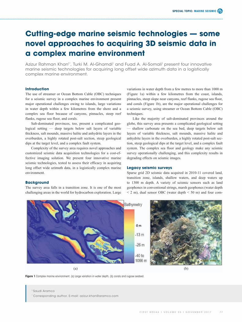
variations in water depth from a few metres to more than 1000 m (Figure 1a) within a few kilometres from the coast, islands, pinnacles, steep slope near canyons, reef flanks, rugose sea floor, and corals (Figure 1b), are the major operational challenges for a seismic survey, using streamer or Ocean Bottom Cable (OBC) techniques.

Like the majority of salt-dominated provinces around the globe, this survey area presents a complicated geological setting — shallow carbonate on the sea bed, deep targets below salt layers of variable thickness, salt mounds, massive halite and anhydrite layers in the overburden, a highly rotated post-salt sec-tion, steep geological dips at the target level, and a complex fault system. The complex sea floor and geology make any seismic survey operationally challenging, and this complexity results in degrading effects on seismic images.

Legacy seismic surveysSparse grid 2D seismic data acquired in 2010-11 covered land, transition zone, islands, shallow waters, and deep waters up to 1300 m depth. A variety of seismic sensors such as land geophones in conventional strings, marsh geophones (water depth < 2 m), dual sensor OBC (water depth < 50 m) and four com-

Cutting-edge marine seismic technologies — some novel approaches to acquiring 3D seismic data in a complex marine environmentAzizur Rahman Khan1*, Turki M. Al-Ghamdi1 and Fuad A. Al-Somali1 present four innovative marine seismic technologies for acquiring long offset wide azimuth data in a logistically complex marine environment.

IntroductionThe use of streamer or Ocean Bottom Cable (OBC) techniques for a seismic survey in a complex marine environment present major operational challenges owing to islands, large variations in water depth within a few kilometres from the shore and a complex sea floor because of canyons, pinnacles, steep reef flanks, rugose sea floor, and corals.

Salt-dominated provinces, too, present a complicated geo-logical setting — deep targets below salt layers of variable thickness, salt mounds, massive halite and anhydrite layers in the overburden, a highly rotated post-salt section, steep geological dips at the target level, and a complex fault system.

Complexity of the survey area requires novel approaches and customized seismic data acquisition technologies for a cost-ef-fective imaging solution. We present four innovative marine seismic technologies, tested to assess their efficacy in acquiring long offset wide azimuth data, in a logistically complex marine environment.

BackgroundThe survey area falls in a transition zone. It is one of the most challenging areas in the world for hydrocarbon exploration. Large

1 Saudi Aramco* Corresponding author, E-mail: [email protected]

Figure 1 Complex marine environment. (a) Large variation in water depth, (b) corals and rugose seabed.

(b)(a)


7 8 F I R S T B R E A K I V O L U M E 3 5 I N O V E M B E R 2 0 1 7

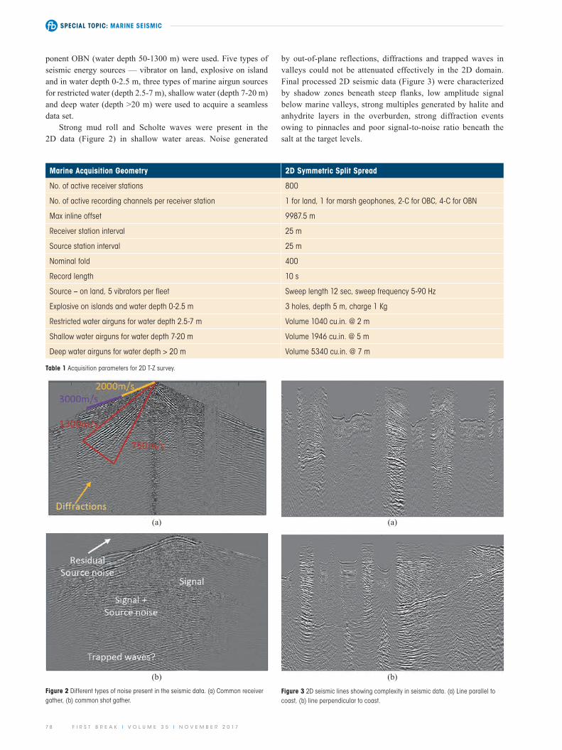
by out-of-plane reflections, diffractions and trapped waves in valleys could not be attenuated effectively in the 2D domain. Final processed 2D seismic data (Figure 3) were characterized by shadow zones beneath steep flanks, low amplitude signal below marine valleys, strong multiples generated by halite and anhydrite layers in the overburden, strong diffraction events owing to pinnacles and poor signal-to-noise ratio beneath the salt at the target levels.

ponent OBN (water depth 50-1300 m) were used. Five types of seismic energy sources — vibrator on land, explosive on island and in water depth 0-2.5 m, three types of marine airgun sources for restricted water (depth 2.5-7 m), shallow water (depth 7-20 m) and deep water (depth >20 m) were used to acquire a seamless data set.

Strong mud roll and Scholte waves were present in the 2D data (Figure 2) in shallow water areas. Noise generated

Marine Acquisition Geometry 2D Symmetric Split Spread

No. of active receiver stations 800

No. of active recording channels per receiver station 1 for land, 1 for marsh geophones, 2-C for OBC, 4-C for OBN

Max inline offset 9987.5 m

Receiver station interval 25 m

Source station interval 25 m

Nominal fold 400

Record length 10 s

Source – on land, 5 vibrators per fleet Sweep length 12 sec, sweep frequency 5-90 Hz

Explosive on islands and water depth 0-2.5 m 3 holes, depth 5 m, charge 1 Kg

Restricted water airguns for water depth 2.5-7 m Volume 1040 cu.in. @ 2 m

Shallow water airguns for water depth 7-20 m Volume 1946 cu.in. @ 5 m

Deep water airguns for water depth > 20 m Volume 5340 cu.in. @ 7 m

Table 1 Acquisition parameters for 2D T-Z survey.

Figure 2 Different types of noise present in the seismic data. (a) Common receiver gather, (b) common shot gather.

Figure 3 2D seismic lines showing complexity in seismic data. (a) Line parallel to coast, (b) line perpendicular to coast.

(b) (b)

(a) (a)



Acquisition geometry and parametersA survey area of size 12 km x 11 km was selected in water depth 600-700 m. Receiver area of size 4 x 3 km was centered at the shot area of 12 x 11 km as shown in the (Figure 5a). All the nodes listened to all the shots. Airgun source with volume 3990 cu. in., pressure 2000 psi and towed at 8 m was fired in flip-flop mode to generate two source lines 50 m apart for every sail line. One addi-tional receiver line with 81 nodes was deployed in 600-1070 m

3D seismic surveys with closer sampling using long offset wide azimuth acquisition geometry were felt necessary for better noise attenuation, suppression of high velocity multiples, and a reliable velocity model building, using Full Wave Form Inversion (FWI) and better migration to improve the image beneath the salt layer. A four-vessel Wide Azimuth (WAZ) long streamer 3D survey in deep waters, with full azimuth up to 4 kilometres, provided a much better image beneath the salt.

Logistical complexity and G&G challenges of the survey area require customized and cost-effective seismic data acquisition technologies. We selected four innovative technologies for their novel approach in marine seismic data acquisition, and tested them in the survey area.

Innovative technologiesThe following four technologies selected for the test:• Marine Autonomous Seismic System – Vendor A• Midwater Stationary Cable System – Vendor B• Floating Node Seismic System – Vendor C• Drifting Node Seismic System – Vendor D

Marine Autonomous Seismic System (MASS) — Vendor Asystem descriptionIt is a node-on-a-rope based Ocean Bottom Node (OBN) system (Figure 4). Its fully automated deployment, retrieval and parallel data downloading make the survey operations and data retrieval highly efficient.

Some of the features of MASS are:• Depth rated to 3000 m (one node type for shallow and deep

waters)• Four-component recording, one hydrophone and three-

component omnidirectional geophones• High weight density for better coupling• Low power consumption electronics for longer battery life up

to 65 days• Built-in sensors for roll and pitch measurement• Stable CSAC clock• Automated battery replacement and system health check• Compact size enables large inventory on a single vessel• Armoured cable with 20 tonne breaking strength

Figure 4 MASS node (image courtesy of Vendor A).

Figure 5 (a) Acquisition geometry (b) Rose plot maximum offset 10.5 km (c) receiver lines on sea bed.

Source line length 12 km

No. of source lines 220

No. of shots per source line 240

Shot interval/Source line interval 50 m

Shot Grid 50 m x 50 m

Receiver line length 4 km

No. of receiver lines 16

Receiver line interval 200 m

No. of nodes per receiver line 81

Node Grid 50 m x 200 m

Bin size 25 m x 25 m

Max fold 1296

Max far offset in-line 8000 m

Max far offset x-line 7000 m

Record length 10 sec

Table 2 Acquisition parameters for MASS test survey.

(b) (c)(a)



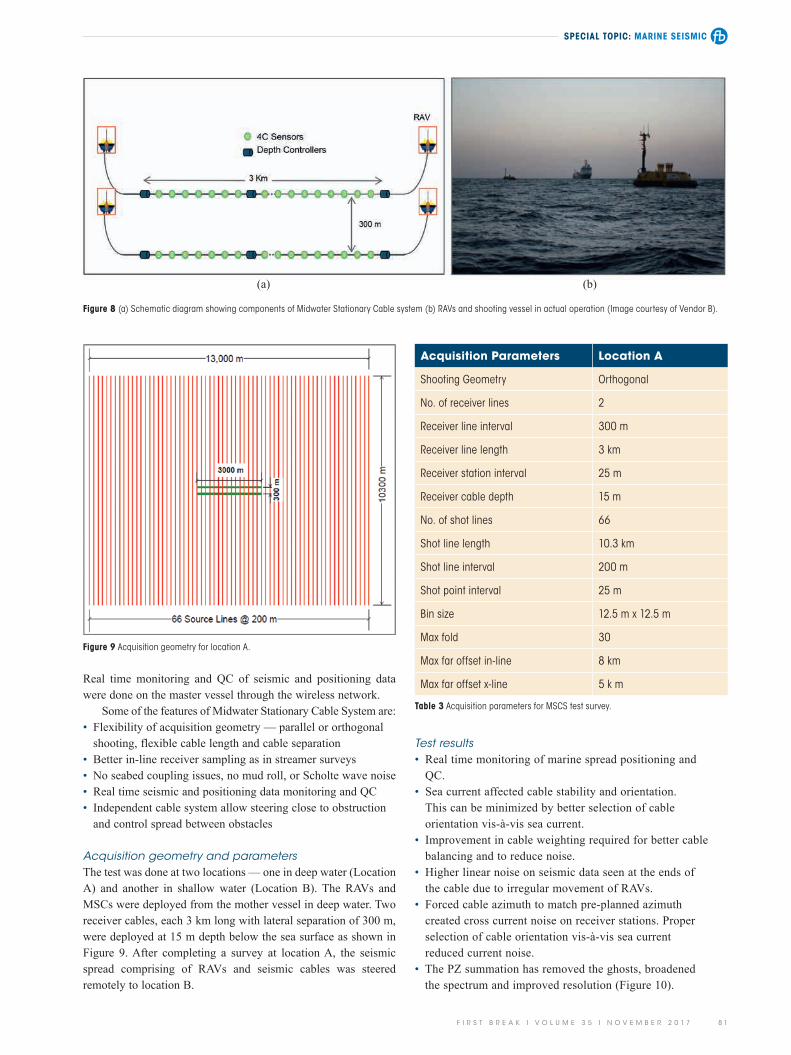
seismic sensors (1 hydrophone and 3 particle motion sensors) at regular intervals of 25 m. Each 4C station has built-in 3-axis inclinometers to compute the orientation of motion sensors (geophones) with respect to vertical. Position of each cable is controlled by a pair of unmanned surface vehicles known as Recording Autonomous Vehicles (RAVs). These RAVs have a small draft of 1.5 m, and are equipped with a seismic recording system, GPS, Gyro, UHF radio transmission and wi-fi system. The armoured lead-in cable connects the seismic cable with RAVs, and dives the seismic cable to a desired depth. Depth controllers maintain neutrally buoyant seismic cables at a desired depth.

Magnetic compasses and acoustic systems are also fitted on the seismic cables to monitor cable shape, cable separation, and to compute receiver position in real time. RAVs keep the cables quasi-stationary in the dynamic sea environment. The master vessel remotely controls the RAVs and steers them to the desired location, maintaining the cable position throughout the survey, while interro-gating the RAVs for real-time data monitoring and QC.

For the test, two cables, each of 3 km long with nominal lateral separation of 300 m, were deployed using four RAVs as shown in the Figure 8. After connecting seismic cables and other equipment, RAVs were steered remotely to the specified location.

water depth (Figure 5c) to test the capability and operational efficiency of the node handling system and positioning accuracy of deployment in deep waters. It was a single vessel operation for both node handling and shooting.

Test results• Survey generated good quality data with max offset up to

10.5 km and full azimuth data up to 4.5 km.• Nodes deployment accuracy in depth range 600-1070 m was

within specifications.• Closer in-line sampling of 50 m helped in better noise sup-

pression and improving image quality.• Dual sensor P-Z summation, standard and RTM migration

improved signal-to-noise ratio by 20 dB and excellent image beneath the salt as seen in Figure 6 (b).

• Survey operation was very efficient with less exposure to HSE risks.

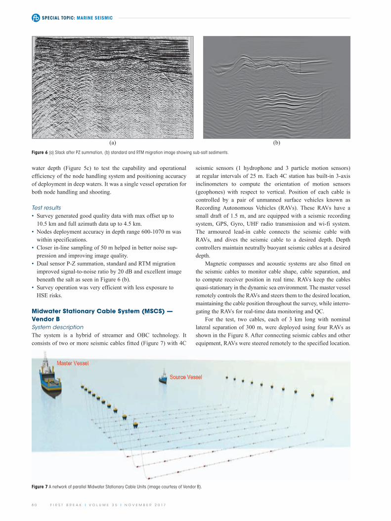
Midwater Stationary Cable System (MSCS) — Vendor BSystem descriptionThe system is a hybrid of streamer and OBC technology. It consists of two or more seismic cables fitted (Figure 7) with 4C

Figure 7 A network of parallel Midwater Stationary Cable Units (image courtesy of Vendor B).

Figure 6 (a) Stack after PZ summation, (b) standard and RTM migration image showing sub-salt sediments.

(b)(a)



Real time monitoring and QC of seismic and positioning data were done on the master vessel through the wireless network.

Some of the features of Midwater Stationary Cable System are:• Flexibility of acquisition geometry — parallel or orthogonal

shooting, flexible cable length and cable separation• Better in-line receiver sampling as in streamer surveys• No seabed coupling issues, no mud roll, or Scholte wave noise• Real time seismic and positioning data monitoring and QC• Independent cable system allow steering close to obstruction

and control spread between obstacles

Acquisition geometry and parametersThe test was done at two locations — one in deep water (Location A) and another in shallow water (Location B). The RAVs and MSCs were deployed from the mother vessel in deep water. Two receiver cables, each 3 km long with lateral separation of 300 m, were deployed at 15 m depth below the sea surface as shown in Figure 9. After completing a survey at location A, the seismic spread comprising of RAVs and seismic cables was steered remotely to location B.

Test results• Real time monitoring of marine spread positioning and

QC.• Sea current affected cable stability and orientation.

This can be minimized by better selection of cable orientation vis-à-vis sea current.

• Improvement in cable weighting required for better cable balancing and to reduce noise.

• Higher linear noise on seismic data seen at the ends of the cable due to irregular movement of RAVs.

• Forced cable azimuth to match pre-planned azimuth created cross current noise on receiver stations. Proper selection of cable orientation vis-à-vis sea current reduced current noise.

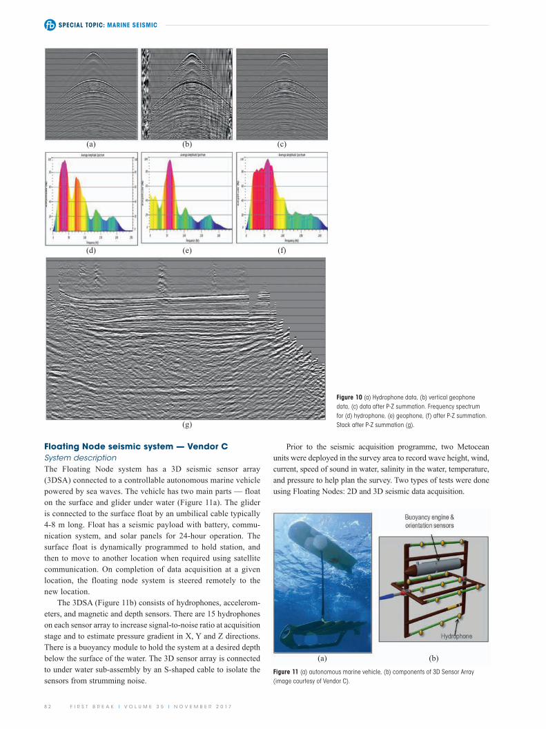
• The PZ summation has removed the ghosts, broadened the spectrum and improved resolution (Figure 10).

Figure 8 (a) Schematic diagram showing components of Midwater Stationary Cable system (b) RAVs and shooting vessel in actual operation (Image courtesy of Vendor B).

Figure 9 Acquisition geometry for location A.

Acquisition Parameters Location A

Shooting Geometry Orthogonal



Receiver line length 3 km

Receiver station interval 25 m

Receiver cable depth 15 m

No. of shot lines 66

Shot line length 10.3 km

Shot line interval 200 m

Shot point interval 25 m

Bin size 12.5 m x 12.5 m

Max fold 30

Max far offset in-line 8 km

Max far offset x-line 5 k m

Table 3 Acquisition parameters for MSCS test survey.

(b)(a)



Prior to the seismic acquisition programme, two Metocean units were deployed in the survey area to record wave height, wind, current, speed of sound in water, salinity in the water, temperature, and pressure to help plan the survey. Two types of tests were done using Floating Nodes: 2D and 3D seismic data acquisition.

Floating Node seismic system — Vendor CSystem descriptionThe Floating Node system has a 3D seismic sensor array (3DSA) connected to a controllable autonomous marine vehicle powered by sea waves. The vehicle has two main parts — float on the surface and glider under water (Figure 11a). The glider is connected to the surface float by an umbilical cable typically 4-8 m long. Float has a seismic payload with battery, commu-nication system, and solar panels for 24-hour operation. The surface float is dynamically programmed to hold station, and then to move to another location when required using satellite communication. On completion of data acquisition at a given location, the floating node system is steered remotely to the new location.

The 3DSA (Figure 11b) consists of hydrophones, accelerom-eters, and magnetic and depth sensors. There are 15 hydrophones on each sensor array to increase signal-to-noise ratio at acquisition stage and to estimate pressure gradient in X, Y and Z directions. There is a buoyancy module to hold the system at a desired depth below the surface of the water. The 3D sensor array is connected to under water sub-assembly by an S-shaped cable to isolate the sensors from strumming noise.

Figure 10 (a) Hydrophone data, (b) vertical geophone data, (c) data after P-Z summation. Frequency spectrum for (d) hydrophone, (e) geophone, (f) after P-Z summation. Stack after P-Z summation (g).

Figure 11 (a) autonomous marine vehicle, (b) components of 3D Sensor Array (image courtesy of Vendor C).

(b)

(g)

(c)(a)

(e) (f)(d)

(b)(a)



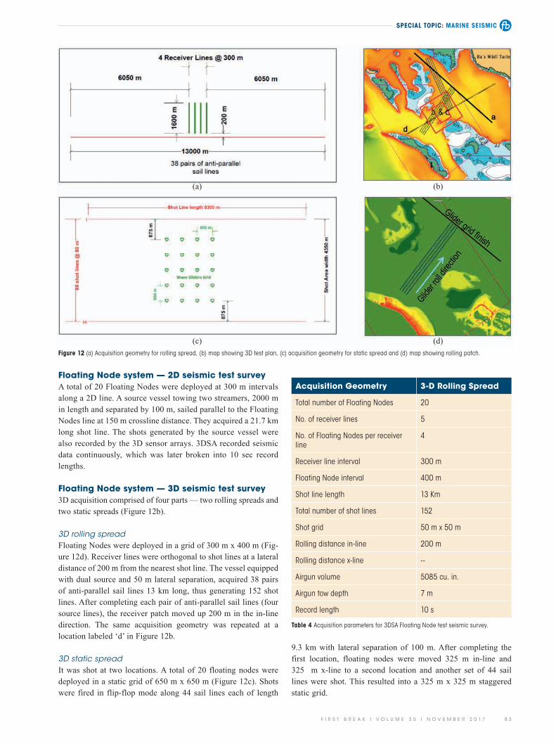
Floating Node system — 2D seismic test surveyA total of 20 Floating Nodes were deployed at 300 m intervals along a 2D line. A source vessel towing two streamers, 2000 m in length and separated by 100 m, sailed parallel to the Floating Nodes line at 150 m crossline distance. They acquired a 21.7 km long shot line. The shots generated by the source vessel were also recorded by the 3D sensor arrays. 3DSA recorded seismic data continuously, which was later broken into 10 sec record lengths.

Floating Node system — 3D seismic test survey 3D acquisition comprised of four parts — two rolling spreads and two static spreads (Figure 12b).

3D rolling spreadFloating Nodes were deployed in a grid of 300 m x 400 m (Fig-ure 12d). Receiver lines were orthogonal to shot lines at a lateral distance of 200 m from the nearest shot line. The vessel equipped with dual source and 50 m lateral separation, acquired 38 pairs of anti-parallel sail lines 13 km long, thus generating 152 shot lines. After completing each pair of anti-parallel sail lines (four source lines), the receiver patch moved up 200 m in the in-line direction. The same acquisition geometry was repeated at a location labeled ‘d’ in Figure 12b.

3D static spreadIt was shot at two locations. A total of 20 floating nodes were deployed in a static grid of 650 m x 650 m (Figure 12c). Shots were fired in flip-flop mode along 44 sail lines each of length

9.3 km with lateral separation of 100 m. After completing the first location, floating nodes were moved 325 m in-line and 325 m x-line to a second location and another set of 44 sail lines were shot. This resulted into a 325 m x 325 m staggered static grid.

Figure 12 (a) Acquisition geometry for rolling spread, (b) map showing 3D test plan, (c) acquisition geometry for static spread and (d) map showing rolling patch.

Acquisition Geometry 3-D Rolling Spread

Total number of Floating Nodes 20


No. of Floating Nodes per receiver line

4


Floating Node interval 400 m

Shot line length 13 Km

Total number of shot lines 152

Shot grid 50 m x 50 m

Rolling distance in-line 200 m

Rolling distance x-line --

Airgun volume 5085 cu. in.

Airgun tow depth 7 m

Record length 10 s

Table 4 Acquisition parameters for 3DSA Floating Node test seismic survey.

(b)

(d)

(a)

(c)



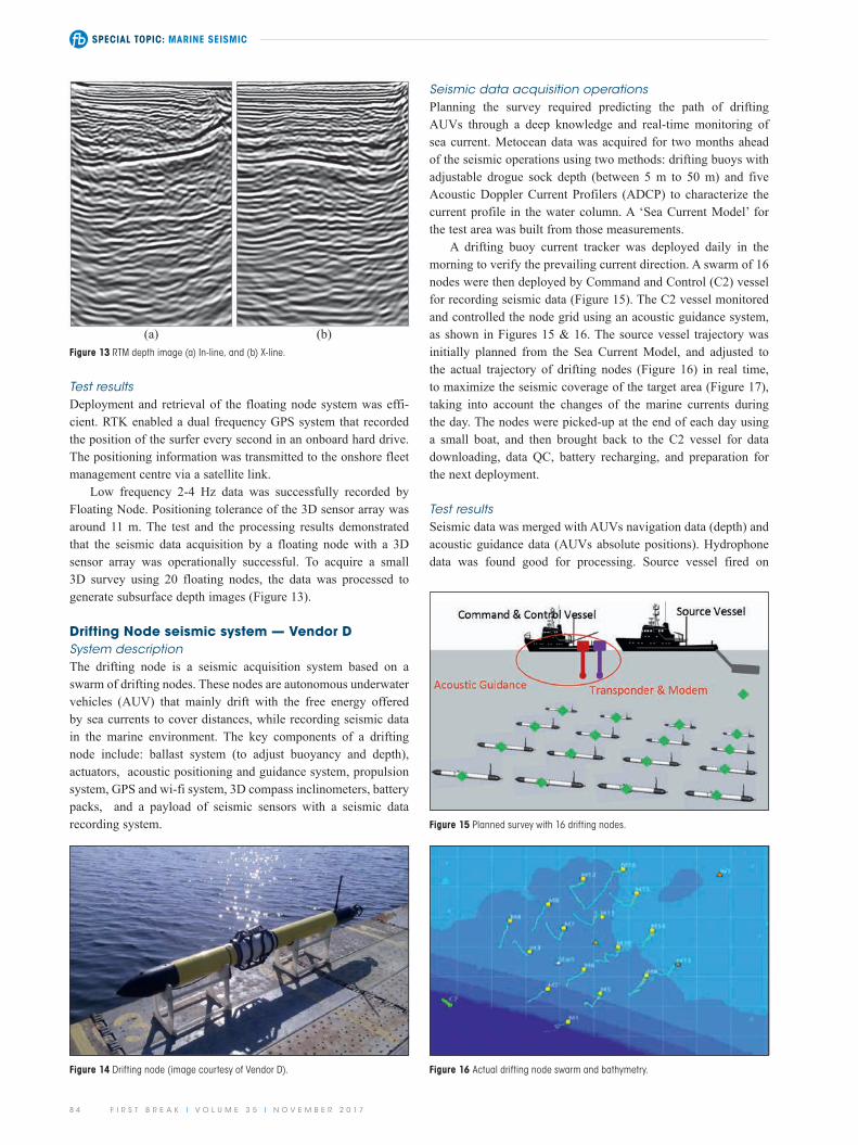
Seismic data acquisition operationsPlanning the survey required predicting the path of drifting AUVs through a deep knowledge and real-time monitoring of sea current. Metocean data was acquired for two months ahead of the seismic operations using two methods: drifting buoys with adjustable drogue sock depth (between 5 m to 50 m) and five Acoustic Doppler Current Profilers (ADCP) to characterize the current profile in the water column. A ‘Sea Current Model’ for the test area was built from those measurements.

A drifting buoy current tracker was deployed daily in the morning to verify the prevailing current direction. A swarm of 16 nodes were then deployed by Command and Control (C2) vessel for recording seismic data (Figure 15). The C2 vessel monitored and controlled the node grid using an acoustic guidance system, as shown in Figures 15 & 16. The source vessel trajectory was initially planned from the Sea Current Model, and adjusted to the actual trajectory of drifting nodes (Figure 16) in real time, to maximize the seismic coverage of the target area (Figure 17), taking into account the changes of the marine currents during the day. The nodes were picked-up at the end of each day using a small boat, and then brought back to the C2 vessel for data downloading, data QC, battery recharging, and preparation for the next deployment.

Test resultsSeismic data was merged with AUVs navigation data (depth) and acoustic guidance data (AUVs absolute positions). Hydrophone data was found good for processing. Source vessel fired on

Test resultsDeployment and retrieval of the floating node system was effi-cient. RTK enabled a dual frequency GPS system that recorded the position of the surfer every second in an onboard hard drive. The positioning information was transmitted to the onshore fleet management centre via a satellite link.

Low frequency 2-4 Hz data was successfully recorded by Floating Node. Positioning tolerance of the 3D sensor array was around 11 m. The test and the processing results demonstrated that the seismic data acquisition by a floating node with a 3D sensor array was operationally successful. To acquire a small 3D survey using 20 floating nodes, the data was processed to generate subsurface depth images (Figure 13).

Drifting Node seismic system — Vendor DSystem descriptionThe drifting node is a seismic acquisition system based on a swarm of drifting nodes. These nodes are autonomous underwater vehicles (AUV) that mainly drift with the free energy offered by sea currents to cover distances, while recording seismic data in the marine environment. The key components of a drifting node include: ballast system (to adjust buoyancy and depth), actuators, acoustic positioning and guidance system, propulsion system, GPS and wi-fi system, 3D compass inclinometers, battery packs, and a payload of seismic sensors with a seismic data recording system.

Figure 14 Drifting node (image courtesy of Vendor D). Figure 16 Actual drifting node swarm and bathymetry.

Figure 13 RTM depth image (a) In-line, and (b) X-line.

Figure 15 Planned survey with 16 drifting nodes.

(b)(a)



source lines of varying length and direction in accordance with the trajectory of drifting nodes, to maximize seismic coverage. Common receiver gathers (Figure 18) recorded while the node was drifting with the current and the source vessel was firing marine airguns. Some elements of internal noise generated by propeller, buoyancy pump and acoustic transponder, were ini-tially observed. This was minimized through synchronization of actuators with seismic recording cycle. The hydrophone’s final PSTM volume shows the top of salt and sediments underneath in Figure 19. Geophone data was recorded but found to be too noisy for processing to contribute to the seismic image.

RecommendationsResults of these tests are very encouraging and all these technol-ogies can be deployed in the near future. Survey area complexity led to testing of these emerging technologies to de-risk seismic operations and acquire seismic data in areas where conventional marine acquisition methods are not suitable. Based on both the test results and equipment availability, Marine Autonomous Seismic System of Vendor A was deployed for a full 3D seismic survey. The other three technologies offer practical solutions and are very promising, but not yet on a scale suitable for a large 3D seismic survey.

AcknowledgementsWe would like to thank Saudi Aramco management for allowing us to publish this work. We express our sincere thanks to the ven-dors for their collaboration and immense support, and particularly the field crew for safe and successful completion of the project.

Figure 18 Hydrophone Common Receiver Gather.

Total no. of active nodes 16


No. of nodes per receiver line 4

Receiver Line Interval 125 m

Receiver Interval 125 m

Shot Line Length variable

Shot interval 20 m

Airgun Volume 3690 cu. in.

Airgun Tow Depth 6 m

Record Length 10 s

A to D conversion 24 bit

Sample interval 2 ms

Table 5 Acquisition parameters for drifting nodes.

Figure 17 Coverage map for offset 0-3000 m.

Figure 19 Hydrophone PSTM stack (a) in-line, and (b) x-line (image courtesy of Vendor D).

(b)(a)

cutting-edge marine seismic technologies — some novel approaches to acquiring 3d ... · sparse...

Documents