currency crisis in developing countries: role of weak...
TRANSCRIPT

International Journal of Arts and Sciences 3(13): 106 - 154 (2010)
CD-ROM. ISSN: 1944-6934 © InternationalJournal.org
106
Currency Crisis in Developing Countries: Role of Weak Fundamentals Maryna Derkach, Vanderbilt University, USA Abstract: The paper examines the determinants of foreign exchange market instabilities in developing countries during the global financial crisis of 2007-2009. Using monthly and annual data for 40 developing economies from 2001 to 2009 we estimate the extent to which the distress in foreign exchange markets could have been explained by weak macroeconomic fundamentals such as overvalued real exchange rates, weak banking systems, and low levels of international reserves. The results of empirical tests supports the idea that high pressure in the foreign exchange market is were partially attributed to the impact of the real exchange rate, lending boom, current account deficit and government expenditure to GDP. The influence of unobservable variables also remains strong. There were empirical evidences that both countries with accumulated macroeconomic misbalances and countries with strong fundamentals were equally vulnerable to adverse external shocks. It has also been found that regional effects were important, and models adjusted for interregional correlation provide better results. Keywords: index of foreign exchange market pressure, currency crises, macroeconomic fundamentals, financial crises 1. Introduction The global financial crisis of 2008 highlighted numerous sources of risk to financial and macroeconomic stability in both developed and developing countries. In advanced economies crisis started from the collapse of the US subprime mortgage market and quickly spread to financial institutions through their exposure to securitized mortgage derivatives. It affected money markets, stock markets and pulled the advanced economies into mild recession starting from the second half of 2007. In September 2008 the financial crisis reached its most critical stage. The decision of the US government to let Lehman Brothers, a large US investment bank, file for bankruptcy triggered market fears that the crisis would worsen; this action provoked a dramatic decline in stock markets.1
Developing economies were hit badly by the crisis
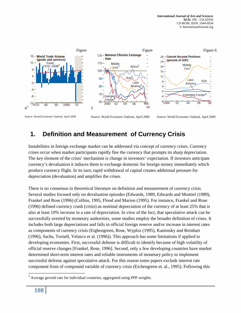
As shown in Figure 1 stock prices fell abruptly in the fall 2008. Consequently, business and consumer confidence diminished (Figure 3) demand and output largely decreased. Tthis way the escalation of the financial crisis inflicted a severe recession in the global economy. In the fourth quarter of 2008 global GDP contracted by 6.5 percent and kept falling in the first quarter of 2009 (Word Economic Outlook, 2009). Industrial production, trade, and employment dropped sharply.
2
1 According to Blanchard (2008) the decrease in the value of the stock markets from July 2007 to November 2008 was equal to $26 400 bln,
through their exposure to shocks from both trade and financial channels. Firstly, world trade volume contracted significantly (Figure 4), and
2 GDP of developing economies fell by 4 percent in the last quarter of 2008.

International Journal of Arts and Sciences 3(13): 106 - 154 (2010)
CD-ROM. ISSN: 1944-6934 © InternationalJournal.org
107
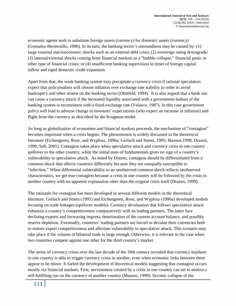
commodity prices fell. Countries faced a decline in export demand and export revenues which worsened their Current Account position (Figure 6). Second, as a result of tightening in the world credit market, investors became more risk adverse, foreign aid declined, and remittances inflows of foreign capital stopped or reversed.
Figure 1
Figure 2
Figure 3
Source: World Economic Outlook, April 2009
Source: World Economic Outlook, April 2009
Source: World Economic Outlook, April 2009
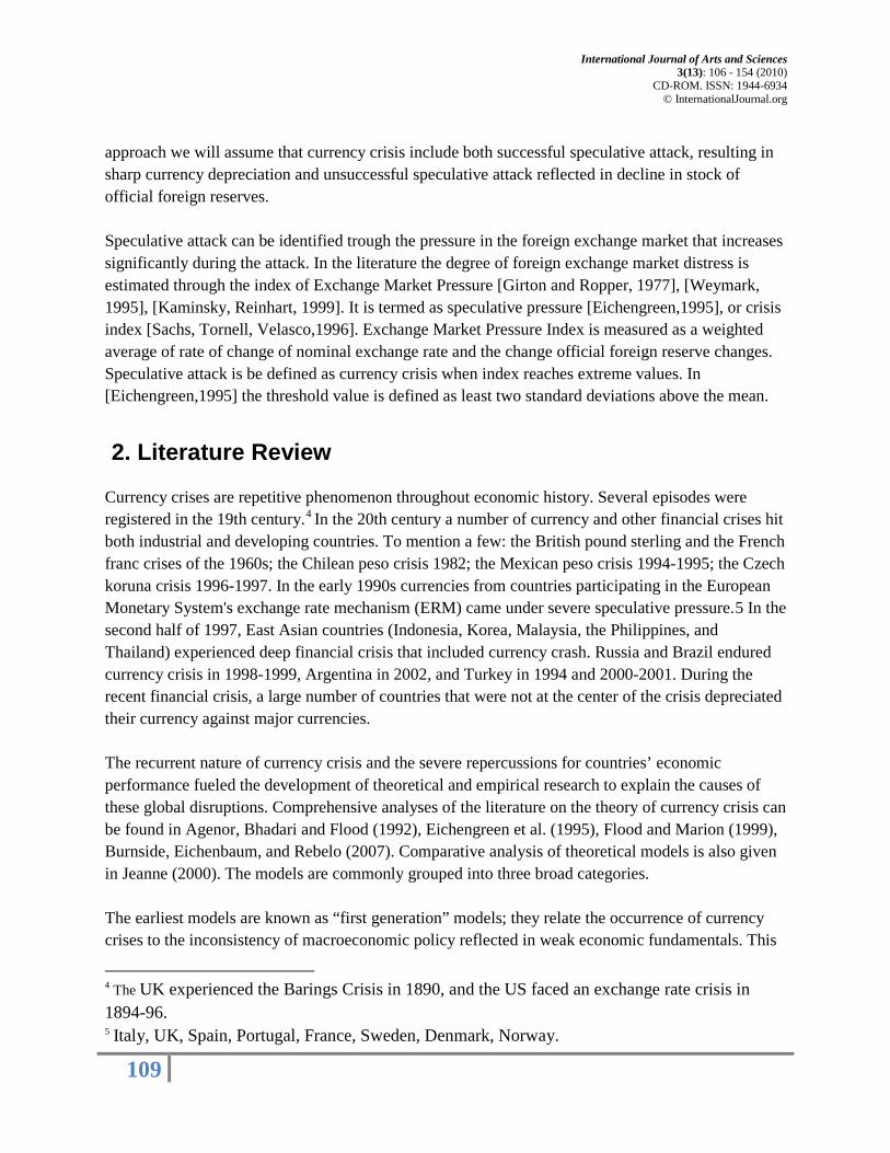
These effects created significant pressure on the foreign exchange markets of developing countries and engender the threat of speculative attacks and currency crises. In the theoretical literature, the origin of a currency crisis is the subject of much debate. Some models suggest that the sudden change in market sentiment and speculative attack are caused by a set of macroeconomic conditions and/or economic policy arrangements. Other models explain speculative attack as a result of regional contagion. As shown in Figure 5, emerging markets faced upward pressure (depreciation) on their currencies soon after September 2008. Yet, the question about whether foreign exchange disturbances developed from weak macroeconomic fundamentals or from cross-country spillovers (contagion) is still unanswered. Our paper research examines the determinants of exchange market pressure in developing countries during the 2008-2009. Using monthly and annual data for 40 developing economies from 2001 to 2009, we estimate the extent to which disturbances in foreign exchange markets could have been explained by weak macroeconomic fundamentals such as overvalued real exchange rates, weak banking systems, and low levels of international reserves. Our objective is to find out the role of macroeconomic fundamentals in investors’ expectations and foreign exchange market stress during and after the financial crises of 2007-2009. The organization of the paper is the following. An overview of theoretical and empirical findings on the causes of currency crises is given in Section II. The empirical model that we develop, the data we use and our econometric procedures are presented in Section III. Results from our regression analysis and robustness checks are discussed in Section IV. Section V provides conclusions.
International Journal of Arts and Sciences 3(13): 106 - 154 (2010)
CD-ROM. ISSN: 1944-6934 © InternationalJournal.org
108
1. Definition and Measurement of Currency Crisis
Instabilities in foreign exchange market can be addressed via concept of currency crises. Currency crises occur when market participants rapidly flee the currency that prompts its sharp depreciation. The key element of the crisis’ mechanism is change in investors’ expectation. If investors anticipate currency’s devaluation it induces them to exchange domestic for foreign money immediately which produce currency flight. In its turn, rapid withdrawal of capital creates additional pressure for depreciation (devaluation) and amplifies the crises. There is no consensus in theoretical literature on definition and measurement of currency crisis. Several studies focused only on devaluation episodes (Edwards, 1989, Edwards and Montiel (1989), Frankel and Rose (1996) (Collins, 1995, Flood and Marion (1995). For instance, Frankel and Rose (1996) defined currency crash (crisis) as nominal depreciation of the currency of at least 25% that is also at least 10% increase in a rate of depreciation. In view of the fact, that speculative attack can be successfully averted by monetary authorities, some studies employ the broader definition of crises. It includes both large depreciations and falls in official foreign reserve and/or increase in interest rates as components of currency crisis (Eighengreen, Rose, Wyploz (1995), Kaminsky and Reinhart (1996), Sachs, Tornell, Velasco et al. (1996)). This approach has some limitations if applied to developing economies. First, successful defense is difficult to identify because of high volatility of official reserve changes [Frankel, Rose, 1996]. Second, only a few developing countries have market determined short-term interest rates and reliable instruments of monetary policy to implement successful defense against speculative attack. For this reason some papers exclude interest rate component from of compound variable of currency crisis (Eichengreen et. al., 1995). Following this 3 Average growth rate for individual countries, aggregated using PPP weights.
Figure
43
Figure
5
Figure 6
Source: World Economic Outlook, April 2009 Source: World Economic Outlook, April 2009 Source: World Economic Outlook, April 2009
International Journal of Arts and Sciences 3(13): 106 - 154 (2010)
CD-ROM. ISSN: 1944-6934 © InternationalJournal.org
109
approach we will assume that currency crisis include both successful speculative attack, resulting in sharp currency depreciation and unsuccessful speculative attack reflected in decline in stock of official foreign reserves. Speculative attack can be identified trough the pressure in the foreign exchange market that increases significantly during the attack. In the literature the degree of foreign exchange market distress is estimated through the index of Exchange Market Pressure [Girton and Ropper, 1977], [Weymark, 1995], [Kaminsky, Reinhart, 1999]. It is termed as speculative pressure [Eichengreen,1995], or crisis index [Sachs, Tornell, Velasco,1996]. Exchange Market Pressure Index is measured as a weighted average of rate of change of nominal exchange rate and the change official foreign reserve changes. Speculative attack is be defined as currency crisis when index reaches extreme values. In [Eichengreen,1995] the threshold value is defined as least two standard deviations above the mean.
2. Literature Review Currency crises are repetitive phenomenon throughout economic history. Several episodes were registered in the 19th century.4 In the 20th century a number of currency and other financial crises hit both industrial and developing countries. To mention a few: the British pound sterling and the French franc crises of the 1960s; the Chilean peso crisis 1982; the Mexican peso crisis 1994-1995; the Czech koruna crisis 1996-1997. In the early 1990s currencies from countries participating in the European Monetary System's exchange rate mechanism (ERM) came under severe speculative pressure.5
In the second half of 1997, East Asian countries (Indonesia, Korea, Malaysia, the Philippines, and Thailand) experienced deep financial crisis that included currency crash. Russia and Brazil endured currency crisis in 1998-1999, Argentina in 2002, and Turkey in 1994 and 2000-2001. During the recent financial crisis, a large number of countries that were not at the center of the crisis depreciated their currency against major currencies.
The recurrent nature of currency crisis and the severe repercussions for countries’ economic performance fueled the development of theoretical and empirical research to explain the causes of these global disruptions. Comprehensive analyses of the literature on the theory of currency crisis can be found in Agenor, Bhadari and Flood (1992), Eichengreen et al. (1995), Flood and Marion (1999), Burnside, Eichenbaum, and Rebelo (2007). Comparative analysis of theoretical models is also given in Jeanne (2000). The models are commonly grouped into three broad categories. The earliest models are known as “first generation” models; they relate the occurrence of currency crises to the inconsistency of macroeconomic policy reflected in weak economic fundamentals. This
4 The UK experienced the Barings Crisis in 1890, and the US faced an exchange rate crisis in 1894-96. 5 Italy, UK, Spain, Portugal, France, Sweden, Denmark, Norway.

International Journal of Arts and Sciences 3(13): 106 - 154 (2010)
CD-ROM. ISSN: 1944-6934 © InternationalJournal.org
110
theoretical approach stems from Krugman’s 1979 paper on the balance of payments model and was developed further by Flood and Garber (1984), Calvo (1987), Drazen and Helpman (1987), and others. Krugman argued that currency crises are a logical consequence of unsustainable exchange rate policy of the government such as the combination of a fixed exchange rate regime and expansionary fiscal and monetary policy.6
Fiscal and monetary expansion drive domestic inflation and prompt investors to trade foreign currency for home currency with the Central Bank until official foreign reserves are exhausted. After some critical point when reserves are too low the speculative attack occurs and the monetary authority is forced to abandon the fixed exchange rate regime and allow the currency to float. Hence, although the most evident cause of currency crises in first generation models is speculation against the currency that cause depletion of foreign reserves, the root of the crises lies in the inconsistency of macroeconomic fundamentals – excessive expansionary fiscal and monetary policy and a fixed exchange rate policy.
It has also been argued in the literature that even sustainable currency pegs may be attacked and broken (Obstfeld, 1994; Eichengreen, Rose, and Wyplosz, 1996). The theory behind this argument is classified as the “second generation of currency crises models.” In this case market participants think the government can defend the fixed exchange rate indefinitely, but they have doubts about the government’s willingness to defend the parity. The authorities may decide to abandon the parity because they are concerned about the adverse consequences of policies needed to maintain the parity (such as higher interest rates) on other key economic variables (such as the level of employment). The government continually compares the costs and benefits of defending the fixed exchange rate versus abandoning it. In this case situation known as multiple equilibrium with self-fulfilling features currency crises take place (Obstfeld, 1994). Countries are able to maintain fixed exchange rate indefinitely in the absence of speculative attack. However, the same countries can face currency crises if subjected to random speculative attacks inflicted by adverse market sentiment. Changes in fundamentals affect the type of equilibrium and the probability of possible successful speculative attacks. The third generation of currency crisis models concentrated on the agenda of financial intermediaries. Abundant empirical evidence supports the idea that the linkage between the onset of currency and banking crises is strong (Kaminski, 1999; Glick and Hutchison, 1999). Financial crisis in emerging markets can be engendered by the banking system and then transmitted to exchange rate markets.7
6 As mentioned in Frankel and Rose (1996), Krugman’s original model was later extended to include a crawling peg (Connolly, 1986) and a currency band (Krugman and Rotenberg, 1991).
Banking as well as debt crisis undermines the trust of both foreign and domestic creditors in the domestic currency and threaten the sustainability of the exchange rate regime. For this reason
7It is also possible that the causality between banking and currency crises works in the reverse order. Currency crises can lead to banking crises (Obstfeld, 1994). Joint causality of the two crises is also well-recognized (Kaminsky and Reinhart, 1999).
International Journal of Arts and Sciences 3(13): 106 - 154 (2010)
CD-ROM. ISSN: 1944-6934 © InternationalJournal.org
111
economic agents seek to substitute foreign assets (currency) for domestic assets (currency) (Gonsalez-Hermosillo, 1996). In its turn, the banking sector’s unsoundness may be caused by: (1) large external macroeconomic shocks such as an external debt crisis; (2) sovereign rating downgrade; (3) internal/external shocks coming from financial markets as a “bubble collapse,” financial panic or other type of financial crises; or (4) insufficient banking supervision in times of foreign capital inflow and rapid domestic credit expansion. Apart from that, the weak banking system may precipitate a currency crisis if rational speculators expect that policymakers will choose inflation over exchange rate stability in order to avoid bankruptcy and other strains on the banking sector (Obstfeld, 1994). It is also argued that a bank run can cause a currency attack if the increased liquidity associated with a government bailout of the banking system is inconsistent with a fixed exchange rate (Velasco, 1987). In this case government policy will lead to adverse change in investors’ expectations (who expect an increase in inflation) and flight from the currency as described by the Krugman model. As long as globalization of economies and financial markets proceeds, the mechanism of “contagion” becomes important when a crisis begins. The phenomenon is widely discussed in the theoretical literature (Eichengreen, Rose, and Wyplosz, 1996a; Gerlach and Smets, 1995; Masson,1999; Drazen, 1999; Sell, 2001). Contagion takes place when speculative attack and currency crisis in one country spillover to the other country, while the initial state of fundamentals gives no sign of a country’s vulnerability to speculative attack. As noted by Drazen, contagion should be differentiated from a common shock that affects countries differently because they are unequally susceptible to “infection.” When differential vulnerability to an unobserved common shock reflects unobserved characteristics, we get true contagion because a crisis in one country will be followed by the crisis in another country with no apparent explanation other than the original crisis itself (Drazen, 1999). The rationale for contagion has been developed in several different models in the theoretical literature. Gerlach and Smets (1995) and Eichengreen, Rose, and Wyplosz (1996a) developed models focusing on trade linkages (spillover models). Currency devaluation that follows speculative attack enhances a country’s competitiveness comparatively with its trading partners. The latter face declining exports and increasing imports, deterioration of the current account balance, and possibly reserve depletion. Eventually, countries’ trading partners are forced to devalue their currencies both to restore export competitiveness and alleviate vulnerability to speculative attack. This scenario may take place if the volume of bilateral trade is large enough. Otherwise, it is relevant in the case when two countries compete against one other for the third country’s market. The series of currency crises over the last decade of the 20th century revealed that currency mayhem in one country is able to trigger currency crisis in another, even when economic links between them appear to be minor. It fueled the development of theoretical models suggesting that contagion occurs mostly via financial markets. First, nervousness created by a crisis in one country can set in motion a self-fulfilling run on the currency of another country (Masson, 1999). Second, collapse of the
International Journal of Arts and Sciences 3(13): 106 - 154 (2010)
CD-ROM. ISSN: 1944-6934 © InternationalJournal.org
112
exchange rate in one country may cause market participants to assign higher probabilities that the crises will occur elsewhere (or in all other countries of the group), even if other countries do not experience similar macroeconomic circumstances. For example, during the Asian Financial Crisis in 1997, not all countries in the group had the same weaknesses that caused currency collapse in Thailand (large current account deficit, slowdown in export growth, appreciation of the real exchange rate, high ratio of short term debt to foreign reserves, under-regulated financial industry and others). For instance, misbalances in Indonesia were much smaller. According to Radelet and Sachs (1998) who focused on the empirical record leading up to the crisis, the current account deficit in Indonesia amounted to 2.5 percent of GDP (lowest of the five East Asian countries8
). Export growth reached 10.4 percent in 1996 (second highest in the region). Credit growth had remained at a much lower level than in the other affected economies. Major corporate bankruptcies were not recorded in Indonesia; its stock market was growing until the crisis started (Radelet and Sachs, 1998). Nevertheless, in September 1997 Indonesia faced the financial crisis as well. One of the main reasons is that investors treated the region as a whole and assumed that if the crisis occurred in Thailand, the other countries in the region would have the same difficulties.
Lastly, investors who incur losses in one country because of a crisis try to cover themselves by liquidating their positions in other countries. The example is the events in several Latin American countries - Brazil, Colombia, Mexico, and Chile -- after the turmoil in the financial market in Russia in 1998. In August 1998 Russian authorities abandoned the currency peg and allowed the rouble to fluctuate in a wider band (that was followed by its significant depreciation). Then they announced a 90 day moratorium on foreign debt servicing. Soon after, in September 2008 the Brazilian stock market experienced huge losses (second largest ever recorded losses on September 1998). As noted by Sell (2001), the huge sales in the equity markets in Brazil reflected the intent of international investors to match the other losses in other financial markets throughout the world. Accordingly, the Brazilian Real steadily declined in value. Given that Brazil followed a currency peg exchange rate regime, the threat of speculative attack was evident. Unable to defend the Real’s target zone against the US dollar, the Brazilian Government decided to let the currency float on January 1998. This overview of the mechanisms of currency crisis development let us define the main causes discussed in the literature. First, currency crises may result from inconsistency in macroeconomic policy such as excessively expansionary fiscal and monetary policies combined with the government’s commitment to defend a fixed exchange rate. Second, a crisis may arise from adverse changes in market sentiments that lead to multiple equilibria and self-fulfilling speculative attack. Third, a bank-run crisis may lead to currency crises either through the loss of credibility for the national currency or the expectation that the government will abandon the fixed exchange rate because of the policies -- loose monetary policy, bank bailouts – the government adopts. Fourth, the occurrence of currency crises may be linked to the phenomenon of contagion.
8 Thailand, Indonesia, Malaysia, South Korea, Philippines were directly hit in the Asian Financial Crisis in 1997.

International Journal of Arts and Sciences 3(13): 106 - 154 (2010)
CD-ROM. ISSN: 1944-6934 © InternationalJournal.org
113
Most of these channels are closely interrelated and may trigger each other. Some research incorporates more than one of these channels in models of currency crisis. One of the broadly cited papers of this kind belongs to Sachs, et al. (1996) who analyzed the aftermath of the Mexico Crisis of 1994-1995 for 20 developing countries. Their objective was to determine whether foreign exchange market disturbances in these countries were mostly attributed to contagion or rooted in fundamental economic weaknesses. It has been argued that the shift in expectations generated by the Mexican crisis induced a pessimistic equilibrium in fundamentally weak countries. We found in Sachs et. al. the following: “the possibility of multiple equilibrium arises because capital movement depends on anticipated exchange rate behavior” (Sachs et al., 1996, p.157). There is joint causality here: devaluation depends on capital outflow, but capital outflow depends on devaluation. The formal model justifying this relationship is described below. The initial conditions are that the government supports an exchange rate peg with nominal exchange rate E0 and real exchange rate E0/P, where P is the ratio of the domestic price level to the foreign price level. For simplicity P is considered equal to 1. K refers to the amount of capital outflow, R – the stock of foreign exchange reserves. The pegged exchange rate regime continues until the government has sufficient reserves to defend the desirable exchange rate parity in the situation of capital outflow. There is no devaluation while K ≤ R. Devaluation occurs if K > R. The next step is for the government to establish a new nominal exchange rate Et to achieve a target real exchange rate. In the next period the nominal exchange rate E1 equals E0 when K ≤ R, and equals (Et - E0)/E0
if K > R.
As argued by Sachs et. al. (1996), the target exchange rate reflects a number of structural variables including the health of the banking system. When the banking sector is sound, the government will set Et
For this reason the target exchange rate is a function of the vulnerability of the banking sector. As suggested by Sachs et. al. (1996), the vulnerability of the banking system can be indirectly assessed by the magnitude of the increase in bank lending during the period preceding crisis (lending boom). Rapid expansion of bank lending diminishes the capability of banks to screen and monitor the business performance and creditworthiness of borrowers with enough precision. It led to an increase in the share of non- performing loans in their portfolios. Apart from that, risky types of loans such as
equal to the long term real exchange rate, e. When the financial condition of the banking sector is weak, the government is more likely to choose a real exchange rate that is depreciated more than e. This reflects the government’s willingness to employ monetary policy measures to stop the currency from depreciating. Theoretically, the government can prevent upward pressure on its currency by keeping the interest rate high. However, an increase in the interest rate might have several undesirable outcomes. It might cause recession accompanied by a growing number of defaults and non-performing loans, and a number of bankruptcies in the banking sector if it is weak. As long as banking crisis has multiple negative repercussions for the economy, governments try to avoid it in most cases. Therefore, it is questionable whether authorities are willing to defend a targeted exchange rate by tightening monetary policy if the banking system is not financially sound.
International Journal of Arts and Sciences 3(13): 106 - 154 (2010)
CD-ROM. ISSN: 1944-6934 © InternationalJournal.org
114
credit card loans and real estate loans grow fast during lending booms. Therefore the target exchange rate is a function of the lending boom as in (11). Et
= e f(LB), f’(LB)> 0, f(0) = 0 (11)
The potential course of the exchange rate is defined in (12):
−
=
0
1)(0
LBfeD E
Devaluation (D) occurs when there is a capital outflow in excess of the level of reserves. The size of the devaluation is greatest when either the exchange rate is initially appreciated to its long run average, so that is high, or there has been a preceding boom in bank lending which means
that f(LB) is high. In the Sachs et. al. (1996) theoretical model, investors exhibit the following behavior: withdraw funds from the country in the event that devaluation, D, is expected to exceed a certain threshold, θ, and maintain funds in the country as long as D is expected to be less than or equal to θ. It is profitable to allocate resources to domestic currency assets as long as the expected depreciation of the currency does not exceed the difference between foreign and domestic interest rates. If there are N investors and each of them holds k assets, then total capital outflow, K, is in (13) below.
=0Nk
K (13)
For any individual investor:
=0kk j
(14) If the exchange rate is not overvalued and banks are not bankrupt (fundamentals are strong), then
=D (e/E0) – f(LB) – 1 and could be very close to zero. Therefore the condition that [(e/E0) – f(LB) – 1] ≤ θ could be satisfied even if θ is small. In this particular situation devaluation, if any, will be smaller than the investors’ threshold for capital flight, and even in the case of devaluation, K will be equal to zero. Since K = 0 < R the devaluation will not occur in this case (see (12)). Contrarily, weak fundamentals will cause [(e/E0) – f(LB) – 1] > θ, investors will withdraw money from the country, and K will be equal to Nk. Whether the devaluation will occur or not depends on the relation between Nk and R. If R is greater then Nk the government will be able to defend exchange rate parity successfully and devaluation will not take place. On the other hand, devaluation might or might not happen if Nk > R, depending on market sentiments. If each investor expects exchange rate stability
if K > R
if K ≤ R
if D > θ
if D ≤ θ
if D > θ
if D ≤ θ
International Journal of Arts and Sciences 3(13): 106 - 154 (2010)
CD-ROM. ISSN: 1944-6934 © InternationalJournal.org
115
(D equal to zero) then he keeps holding domestic currency assets (k = 0) and no devaluation will occur. But if each investor expects devaluation, then K = Nk > R, and devaluation will take place. In this case devaluation is a self-fulfilling prophecy. Sachs et al.’s (1996) theoretical model captures three generations of models of currency crisis. Its main idea is to explain exchange market pressure as a result of self-fulfilling panic based on the existence of multiple equilibria (second generation). Their theoretical framework is built upon the analysis of the influence of the banking sector (financial channel); and also refers to the role of macroeconomic conditions in crisis scenarios (first generation); and includes the influence of contagion. The theoretical framework corresponds to the objective of our study. On the one hand, exchange market disturbances in developing countries during the global financial crisis of 2008-2009 were at least partially attributed to the financial channel. On the other hand, a theoretical framework which allows for the influence of fundamentals and contagion is very relevant to our study of the role played by fundamentals in the magnitude of foreign exchange market disturbances in developing countries during crises. Therefore we use the Sachs et. al. (1996) model as our benchmark theoretical model.
Empirical Models of Currency Crisis
Various approaches have been used in the empirical literature to model and predict currency crises. Overviews of the methodologies and variables used to characterize crisis episodes can be found in Kaminsky, Lizondo, and Reinhart (1997), Berg and Patillo (1998), and Yan (2001). Kaminsky, Lizondo, and Reinhart (1997) completed a comprehensive survey of empirical studies from 1979 to 1996 on currency crises and summarized information on countries studied, sample size, data frequency, methodology and the main variables used as indicators of crises. Yan (2001) expanded their overview by adding summaries of research conducted from 1999 to 2000. In this section we provide a brief outline of the benchmark studies and broaden the overview of the empirical literature on currency crises with recent findings. According to Kaminsky, Lizondo, and Reinhart (1997) most of the empirical research on currency collapse builds upon one of four different methodological approaches. The first one is qualitative analysis of crisis episodes. The authors investigate the behavior of countries before and during the crisis and seek to distinguish its common patterns and causes. Formal tests to validate the results of theoretical models are usually not performed. Within this framework Goldstein (1996) examined episodes in Argentina, Brazil, Chile and Mexico asking why some countries are more vulnerable than others to the same exogenous shock (Mexico crisis 1994-1995). Dornbush, Goldfajn and Valdes (1995) reviewed currency collapses in Mexico in 1982 and 1994, Chile in early 1980 and Finland in 1992 which, as the authors claimed, share common features -- domestic currency overvaluation, large external deficit, lending boom , deep recession after the crises. The objective of the paper was to

International Journal of Arts and Sciences 3(13): 106 - 154 (2010)
CD-ROM. ISSN: 1944-6934 © InternationalJournal.org
116
identify the common factors that ultimately led to crises. They found that all countries in the group experienced real exchange rate appreciation, deterioration of current account, heavy external borrowing, distress of the financial system, inflation stabilization programs and high interest rates. The second approach can be found in Eichengreen, Rose, and Wyplosz (1996) and Frankel and Rose (1996). They analyze either the evolution of the crisis indicators in the periods preceding and following the crisis (Frankel, Rose, 1996) or compare the behavior of macroeconomic and financial variables around the time of the crises with a control group of “non crisis” cases (Eichengreen et al., 1995). The movement of the each variable such as the rate of growth of domestic credit, the government budget as a fraction of GDP, and so forth is plotted on separate graphs. This way information about the behavior of each indicator can be summarized. However, event study does not allow for interdependencies among the indicators, which is a disadvantage. On the basis of their graphical analysis, Frankel and Rose (1996) found that countries that suffered from currency crises tend to have: (1) a high proportion of their debt lent by commercial banks, (2) a high proportion of their debt on variable rate terms and in short maturities and (3) and a relatively low fraction of the debt that is concessional, lent by multilateral organizations or lent to the public sector. All these indicators are considered as “high” or “low” comparatively to tranquil observations. Countries with currency crises attract disproportionately small inflows of foreign direct investment (FDI). They also revealed that in the period preceding the crisis: (4) foreign interest rates tend to be high, and economic growth in north hemisphere countries is low. The most vulnerable countries tend to have: (5) overvalued currencies (more than 10%); (6) high and rising debt burden; (7) and falling and low international reserves. Analyzing the impact of current account and budget deficit the authors found that both indicators do not vary significantly in the periods preceding crises in comparison with tranquil times. The notable conclusion that was made in this study is that most variables except the real exchange rate and the growth rate of real output per capita move very sluggishly in the years before and after the crisis. This makes this method inappropriate for accurate prediction of the timing of a crisis. The other group of empirical methods uses the “signal approach” (Kaminsky, Lizondo, and Reinhart (KLR), 1998). Their study is also based on event study methodology and expands it further. The authors analyze the behavior of variables that were found significant in previous empirical research on currency crises and develop a technique to recognize the most effective predictors of the crisis. An indicator is regarded as a “warning” signal whenever it departs from its mean beyond a given threshold level. The threshold level is calculated so as to strike a balance between the risk of having too many false signals and the risk of missing many crises. The indicators that were found to be useful in the prediction of currency crises include exports, deviations of the real exchange rate from trend, the ratio of broad money to gross international reserves, domestic credit, credit to the public

International Journal of Arts and Sciences 3(13): 106 - 154 (2010)
CD-ROM. ISSN: 1944-6934 © InternationalJournal.org
117
sector, and domestic inflation. Trade balance, export performance, money growth, real GDP growth, and fiscal deficit have also been used. A third group of papers focused on predicting the timing and magnitude of a crisis by estimating the one-period-ahead probability of devaluation. These studies employ the logit or probit model for empirical analysis. One of the first papers using this framework was by Blanco and Garber (1986) who analyzed the Mexican experience during 1973-1982; they produced time series estimates of peso devaluation through the fourth quarter of 1973 to the third quarter of 1982 as well as the expected exchange rates conditional on devaluation. Since then these methods are used both in studies of crises in a single country (Ferudun, 2008) and for a sample of countries (Frankel and Rose, 1996; Ötker and Pazabaşioĝlu, 1997; Yan 2002). An estimation of the impact of the regressors on the probability of a crash with a probit model using maximum likelihood was also performed by Frankel and Rose in the study mentioned above (1996). The results were reported as the effect of a one unit change in the regressor on the probability of a crash expressed in percentage points. They found that currency crises are more likely occur when FDI flows dry up, reserves are low, domestic credit growth is high, interest rates in the northern hemisphere rise, and the real exchange rate is overvalued. The role of the current account and the government budget deficit in currency crash were not supported by the data. Ötker and Pazabaşioĝlu (1997) analyzed the role of macroeconomic fundamentals in episodes of foreign exchange market pressure 1992-1993 for six European countries (Belgium, Denmark, France, Ireland, Italy, Spain) during the period 1975-1995. They choose an economic policy measure – change in the exchange rate regime - as a dependent variable and a set of variables derived from the monetary approach to the balance of payments model to assess the one-step-ahead probability of a change of regime. The empirical results suggested that, for a majority of the sample countries, episodes of speculative pressures and observed regime changes are associated with deterioration in economic fundamentals. In particular, expansionary credit policies and a widening of government deficits appear to trigger speculative attacks and contribute to an increase in the probability of devaluations. However, in the case of Denmark and, to some extent, France it was found that a relatively small portion of the speculative pressures detected by the pressure indicators can be attributed to the deterioration in economic fundamentals. Therefore the authors concluded that consistent fundamentals are necessary but not sufficient to ensure the maintenance of stable exchange rates. That might also imply that the observed regime changes in these countries were triggered by other factors not captured by the monetary model. Almost similar results were obtained by Kruger, Osakwe, and Page (1998) in their study of the determinants of currency crises in Latin American, Asian and African countries. They used probit approach to analyze pooled annual data for 19 developing countries spanning from 1977 to 1993. Their empirical findings indicate that such fundamental macroeconomic variables as lending boom, real exchange rate misalignment, and reserve inadequacy increase the probability of speculative
International Journal of Arts and Sciences 3(13): 106 - 154 (2010)
CD-ROM. ISSN: 1944-6934 © InternationalJournal.org
118
attack on the currency. Yet, currency crises can not be explained solely by looking at economic fundamentals and regional contagion; speculative behavior of investors is also important. Both logit and probit models are used when the dependent variable is categorical, including variables with binary response. In modeling currency crises, the observable outcome is equal to one if a crisis occurred and equal to zero if it did not occur at that point in time. The event “crisis” is identified when a latent variable such as an index of foreign exchange market pressure exceeds a certain threshold such as 1.5 or 2 standard deviations above its mean. However, there is great diversity in the literature regarding the methodology for constructing the exchange market pressure index.9 In some papers the index is a weighted average of rates of change of the nominal exchange rate, foreign exchange reserves, and the interest rate (Eihengreen, Rose, and Wyplosz, 1996)10
. In others the index is constructed as a weighted average of nominal exchange rate devaluation and the change in official exchange reserves (Sachs et al., 1996). There is discussion in the literature regarding the way to assign weights to components of an index. And lastly, there is also no consensus on the value of the threshold above which a country is considered to enter the crisis. The index of foreign exchange market pressure determines the number of crises episodes identified within the same time framework for the same group of countries and influences the results obtained in the modeling.
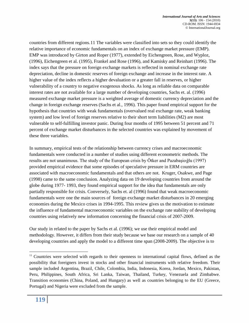
Both the signal approach and probit methodology (if applied to a panel of countries) are based on an assumption that all crises are explained by the same theoretical model (Berg and Patillo, 1998). For instance, Glick and Hutchison (1999) estimated the probability of either currency or banking crisis using a multivariate probit model on a dataset for 90 industrial and developing countries over the 1975 – 1997 period. They observed that either the country at a particular time (observation t) was experiencing crisis (the binary dependent variable yt = 1) or not (yt = 0). The probability that the crisis occurs, Pr (yt
= 1), was hypothesized to be a function of characteristics associated with observation t, xt , and the parameter vector β. The log of the likelihood function (15) is maximized with respect to the unknown parameters and over n observations.
(15) They found that the probability of a crisis rises with greater real overvaluation, a higher ratio of the log of M2 to reserves, and lower export growth. The alternative approach to currency crisis modeling can be found in Sachs et al. (1996). Their methodology is based on cross section multivariate OLS regression for a sample of 20 developing
9 The intuition behind the index is that when a currency experiences high downward pressure (depreciation), monetary authorities can respond by devaluating the currency, running down official foreign exchange reserves, or increasing interest rates. 10 Weights are chosen as long as the volatility of reserves, interest rates and exchange rates are different in order to prevent any of the series from dominating the index.
International Journal of Arts and Sciences 3(13): 106 - 154 (2010)
CD-ROM. ISSN: 1944-6934 © InternationalJournal.org
119
countries from different regions.11
The variables were classified into sets so they could identify the relative importance of economic fundamentals on an index of exchange market pressure (EMP). EMP was introduced by Girton and Roper (1977), extended by Eichengreen, Rose, and Wyploz, (1996), Eichengreen et al. (1995), Frankel and Rose (1996), and Kamisky and Reinhart (1996). The index says that the pressure on foreign exchange markets is reflected in nominal exchange rate depreciation, decline in domestic reserves of foreign exchange and increase in the interest rate. A higher value of the index reflects a higher devaluation or a greater fall in reserves, or higher vulnerability of a country to negative exogenous shocks. As long as reliable data on comparable interest rates are not available for a large number of developing countries, Sachs et. al. (1996) measured exchange market pressure is a weighted average of domestic currency depreciation and the change in foreign exchange reserves (Sachs et al., 1996). This paper found empirical support for the hypothesis that countries with weak fundamentals (overvalued real exchange rate, weak banking system) and low level of foreign reserves relative to their short term liabilities (M2) are most vulnerable to self-fulfilling investor panic. During four months of 1995 between 51 percent and 71 percent of exchange market disturbances in the selected countries was explained by movement of these three variables.
In summary, empirical tests of the relationship between currency crises and macroeconomic fundamentals were conducted in a number of studies using different econometric methods. The results are not unanimous. The study of the European crisis by Ötker and Pazabaşioĝlu (1997) provided empirical evidence that some episodes of speculative pressure in ERM countries are associated with macroeconomic fundamentals and that others are not. Kruger, Osakwe, and Page (1998) came to the same conclusion. Analyzing data on 19 developing countries from around the globe during 1977- 1993, they found empirical support for the idea that fundamentals are only partially responsible for crisis. Conversely, Sachs et. al (1996) found that weak macroeconomic fundamentals were one the main sources of foreign exchange market disturbances in 20 emerging economies during the Mexico crises in 1994-1995. This review gives us the motivation to estimate the influence of fundamental macroeconomic variables on the exchange rate stability of developing countries using relatively new information concerning the financial crisis of 2007-2009. Our study in related to the paper by Sachs et al. (1996); we use their empirical model and methodology. However, it differs from their study because we base our research on a sample of 40 developing countries and apply the model to a different time span (2008-2009). The objective is to
11 Countries were selected with regards to their openness to international capital flows, defined as the possibility that foreigners invest in stocks and other financial instruments with relative freedom. Their sample included Argentina, Brazil, Chile, Colombia, India, Indonesia, Korea, Jordan, Mexico, Pakistan, Peru, Philippines, South Africa, Sri Lanka, Taiwan, Thailand, Turkey, Venezuela and Zimbabwe. Transition economies (China, Poland, and Hungary) as well as countries belonging to the EU (Greece, Portugal) and Nigeria were excluded from the sample.

International Journal of Arts and Sciences 3(13): 106 - 154 (2010)
CD-ROM. ISSN: 1944-6934 © InternationalJournal.org
120
estimate to what extent variation in the exchange market distress across developing countries during the recent global financial crisis can be explained by differences in fundamental macroeconomic conditions in these countries.
4. Model and Data
Our empirical model shows the impact of real exchange rate (RER) misalignment and lending boom (LB) on an index of foreign exchange market pressure (EMP) for countries with weak and strong fundamental macroeconomic conditions. The index of foreign exchange market pressure is a weighted average of the monthly rate of depreciation of a country’s nominal exchange rate with respect to the US dollar and the monthly rate of depletion of a country’s official reserves.12
A higher value of the index signifies more disturbance in the country’s foreign exchange market. In the Sachs et. al. (1996) model, weights are applied to each series for each country and are based on the relative precision (the inverse of the variance) of each series over the ten years before the period under examination (Sachs et. al, 1996). However, more recent empirical studies showed that precision weights can generate substantial biases in the measure of exchange market pressure (Li, Rajan, Willet, 2006). One alternative is to assign equal weights to both components of the index. We adopt this approach and calculate the index of foreign exchange market pressure as the summation of the change in the nominal exchange rate and the change in official foreign exchange reserves assuming that precision weights are both equal to 1.
Our explanatory variables are misalignment of the real exchange rate (RER), lending boom (LB); and each of them in interaction with dummy variables, DLR and DWF. The dummy variables identify groups of countries with fundamental macroeconomic misbalances. In our definition of the dummy variables we follow Sachs et al. (1996) methodology. Countries are classified as strong or weak on fundamentals by ranking them with regard to the degree of misalignment of the real exchange rate (RER), the weakness of the banking system (LB) and the abundance of foreign reserves (M2/R). A country is considered to have strong fundamentals if its real depreciation is in the highest quartile of the sample (the most depreciated currencies) and its lending boom is in the lowest quartile (the lowest ratio of domestic credit growth to GDP). Countries with low fundamentals have a weak banking system and an overvalued exchange rate. We identify these groups of countries with a dummy variable Dwf equal to one if the fundamentals are weak and 0 if they are strong. Abundance/dearth of foreign exchange reserves is measured via reserves adequacy, which is the ratio of the money stock to the level of foreign reserves (M2/R). This coefficient provides more accurate measure of reserve sufficiency than its volume or the ratio of a country’s foreign exchange reserves to GDP. (Calvo, 1987; Sachs et al., 1996). We ranked all countries in our sample according to the value of M2/R in decreasing order. If the country’s ratio of M2 to R belongs to the lowest quartile, it 12 Depletion of official reserves is the monthly percentage change in reserves taken with a negative sign.

International Journal of Arts and Sciences 3(13): 106 - 154 (2010)
CD-ROM. ISSN: 1944-6934 © InternationalJournal.org
121
is considered to have a high level of foreign reserves. For all other countries reserves are relatively low. A second dummy variable DLR takes a value of one if the country has a high level of foreign reserves and zero otherwise. Our final empirical model is given in (16) below: EMP = β1 + β2 (RER) + β3 (LB) + β4 (DLR * RER) + β5 (DLR * LB) + β6 (DLR * DWF * RER) + β7 (DLR * DWF * LB) (16) We obtain the following from this model: • (β2 and β3) represent the effects of fundamentals on the crisis index for the countries with high reserves (DLR =0) and strong fundamentals (DWF=0); • (β2 + β4) and (β3 + β5) capture the effects of fundamentals on the crisis index for countries with low reserves (DLR=1) but strong fundamentals (DWF=0); • (β2 +β4 + β6) and (β3 +β5 + β7) refer to the effects of fundamentals on the crisis index for the countries with low reserves and weak fundamentals.
The main hypothesis of our model is that speculative crisis occurs only when both fundamentals are weak and reserves are low. Therefore we expect that β2 = 0; β2+ β4 = 0; β2 +β4 + β6 < 0. Countries with appreciated real exchange rate suffer more severe crisis, but this only matters for countries with low reserves and weak fundamentals. β3 = 0; β3 +β5 = 0; β3 +β5 + β7 > 0. Increase in lending magnifies the exchange market pressure, but only for countries with low reserves and weak fundamentals. Sachs et. al. (1996) tested these hypotheses on the sample of 20 emerging economies that they thought were exposed to international capital flows in 1995. More than one third of the sample was in Latin America and more than one third in East and South Asia countries. The other regions were weakly represented. The core idea of the paper was that countries in the same geographic area respond differently to the same exogenous shock depending on their internal conditions and previously accumulated misbalances. Since the paper was published, financial markets and institutions in developing countries have changed. First, new financial markets (China, Russia, Poland) were established. Second, the volume of trade, the level of international financial integration, and the degree of financial penetration increased dramatically. These are excellent reasons to revisit the Sachs et. al. model today and to reassess the importance of economic fundamentals and interregional linkages in predicting currency crises in emerging markets.13
13 Our sample allows us to group countries into six different regions: Latin America, East Asia,
South Asia, Eastern and Central Europe, CIS countries, and Africa.
International Journal of Arts and Sciences 3(13): 106 - 154 (2010)
CD-ROM. ISSN: 1944-6934 © InternationalJournal.org
122
We estimate the influence of macroeconomic fundamentals (overvalued exchange rate and lending boom) on the magnitude of foreign exchange market pressure in 40 developing economies during the eight month period from October 2008 to June 2009 when the global financial crisis was in full swing and the global recession was the deepest. We check the robustness of the results to the specification of the variables, and we adjust the model for intraregional correlation of the residuals.
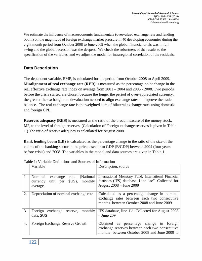
Data Description The dependent variable, EMP, is calculated for the period from October 2008 to April 2009. Misalignment of real exchange rate (RER) is measured as the percentage point change in the real effective exchange rate index on average from 2001 – 2004 and 2005 - 2008. Two periods before the crisis started are chosen because the longer the period of over-appreciated currency, the greater the exchange rate devaluation needed to align exchange rates to improve the trade balance. The real exchange rate is the weighted sum of bilateral exchange rates using domestic and foreign CPI. Reserves adequacy (RES) is measured as the ratio of the broad measure of the money stock, M2, to the level of foreign reserves. (Calculation of Foreign exchange reserves is given in Table 1.) The ratio of reserve adequacy is calculated for August 2008. Bank lending boom (LB) is calculated as the percentage change in the ratio of the size of the claims of the banking sector in the private sector to GDP (B/GDP) between 2004 (four years before crisis) and 2008. The variables in the model and data sources are given in Table 1. Table 1: Variable Definitions and Sources of Information Variable Description, source
1 Nominal exchange rate (National currency unit per $US), monthly average.
International Monetary Fund, International Financial Statistics (IFS) database. Line “ae”. Collected for August 2008 – June 2009
2. Depreciation of nominal exchange rate Calculated as a percentage change in nominal exchange rates between each two consecutive months between October 2008 and June 2009
3 Foreign exchange reserve, monthly data, $US
IFS database, line 1ld. Collected for August 2008 – June 209
4. Foreign Exchange Reserve Growth Obtained as percentage change in foreign exchange reserves between each two consecutive months between October 2008 and June 2009 to
International Journal of Arts and Sciences 3(13): 106 - 154 (2010)
CD-ROM. ISSN: 1944-6934 © InternationalJournal.org
123
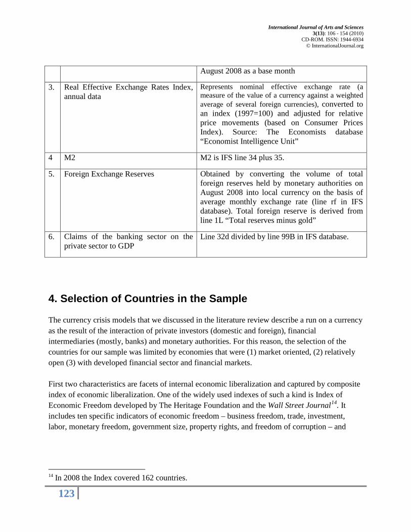
August 2008 as a base month
3. Real Effective Exchange Rates Index, annual data
Represents nominal effective exchange rate (a measure of the value of a currency against a weighted average of several foreign currencies), converted to an index (1997=100) and adjusted for relative price movements (based on Consumer Prices Index). Source: The Economists database “Economist Intelligence Unit”
4 M2 M2 is IFS line 34 plus 35.
5. Foreign Exchange Reserves Obtained by converting the volume of total foreign reserves held by monetary authorities on August 2008 into local currency on the basis of average monthly exchange rate (line rf in IFS database). Total foreign reserve is derived from line 1L “Total reserves minus gold”
6. Claims of the banking sector on the private sector to GDP
Line 32d divided by line 99B in IFS database.
4. Selection of Countries in the Sample
The currency crisis models that we discussed in the literature review describe a run on a currency as the result of the interaction of private investors (domestic and foreign), financial intermediaries (mostly, banks) and monetary authorities. For this reason, the selection of the countries for our sample was limited by economies that were (1) market oriented, (2) relatively open (3) with developed financial sector and financial markets. First two characteristics are facets of internal economic liberalization and captured by composite index of economic liberalization. One of the widely used indexes of such a kind is Index of Economic Freedom developed by The Heritage Foundation and the Wall Street Journal14
14 In 2008 the Index covered 162 countries.
. It includes ten specific indicators of economic freedom – business freedom, trade, investment, labor, monetary freedom, government size, property rights, and freedom of corruption – and

International Journal of Arts and Sciences 3(13): 106 - 154 (2010)
CD-ROM. ISSN: 1944-6934 © InternationalJournal.org
124
weighted15. Countries classified as free have minimal government interference in the economy. Countries with repressed freedom are mostly characterized by violated property rights, high corruption, government control of industries and/or the banking system, monetary instability, and lack of investment freedom. We assume that foreign capital tends to avoid countries with underdeveloped markets, poor market infrastructure, and inefficient institutions. For this reason the original sample of 136 developing countries16
is narrowed to 93 by excluding not rated low and low middle income countries with repressed or mostly repressed economic freedom.
In developing countries success in economic reform and development may be spread unequally among the different sectors of the economy. Some countries might have a favorable investment climate and a relatively developed financial sector, but lag behind in terms of the size of the public sector or regulation of monopolies. In order to capture such countries we have also examined whether they are rated or not rated by Standard and Poor’s, one of the world’s leading credit rating agencies.17
The list of low income and lower middle income economies that do not achieve economic freedom are reported in Appendix 1, Table 6. It is shown that some of the countries are rated while others are not. Rated countries were added to the sample.
To access the level of countries’ financial development we use the methodology suggested by Demirguc-Kunt and Levine (2001). Because one of the main functions of financial intermediaries is to channel savings to investors, they used (1) the ratio of domestic credit provided by the banking sector to GDP18
15 The Index values range from a low of 0 to a high of 100; all countries are ranked and defined as “Free” (80-100), “Mostly free” (70-79.9), “Moderately free” (60-69.9), “Mostly unfree” (50-59.9), “Repressed” (0-49.9).
and (2) the total value of traded stocks to GDP as measures of the activity of financial intermediaries and the equity market. Both variables differ considerably across countries in different income per capita groups. Higher income countries tend to have a more developed financial sector measured in terms of the size, activity and efficiency of banks, non-bank financial institutions and equity markets. Demirguc-Kunt and Levine define the country’s financial sector as underdeveloped if (1) the ratio of domestic credit provided by the banking sector to GDP is less than the sample mean calculated for all countries
16 Our initial sample included all low income, lower-middle and upper-middle income economies, defined according to World Bank criteria. All countries with GNI per capita below $11905 belong to this group (144 countries). Countries with long-term civil war or large-scale breakdown of the rule of law were not included in the sample (Afghanistan, Haiti, Somalia, Myanmar, Iraq, Zimbabwe); we also exclude non-development-oriented dictatorships (North Korea, Cuba). 17 We used Sovereign local currency ratings and sovereign foreign currency ratings issued by Standard & Poor’s as of January 26, 2010. 18The ratio of domestic credit provided by the banking sector to GDP is defined as the financial resources provided to the private sector, such as loans, purchases of non-equity securities, trade credits and other accounts receivable, that establish a claim for repayment.
International Journal of Arts and Sciences 3(13): 106 - 154 (2010)
CD-ROM. ISSN: 1944-6934 © InternationalJournal.org
125
belonging to the same income per capita group, and (2) the total value of traded stocks to GDP is less than the sample mean. A country’s financial system is considered financially underdeveloped if it has both a poorly developed banking sector and equity markets. To define the relative level of financial development for the developing countries we computed mean values for both indicators for each of three country groups by per capita income (Low income, Low middle income, Upper middle income).19
The low middle income group averages 22.5 percent (domestic credit variable) and 6.51 percent (traded stocks variable); the upper middle income group averages 36.72 percent and 12.33 percent. The results are reported in Appendix 1, Tables A.2 and A.3. Within the group of lower middle income countries, indicators of the banking system and non-bank financial intermediaries or equity markets exceed the mean for 21 countries, so we add an additional five countries to our sample.
Application of the same methodology to the upper middle income countries meet some limitations. Our calculations shows that the mean values for this group increase to 52.2 percent of GDP for financial intermediaries and 22.2 percent of GDP for the stock market (Appendix1, Table 9). Consequently, several countries with relatively developed equity markets and a financial sector (Argentina, Poland, and Turkey) did not fit into the sample selection criteria. It may refer to the fact that countries with less mature financial systems and inappropriate financial supervision may produce a much higher level of domestic credit to GDP than countries with more developed financial systems and better macroeconomic management. For instance, Poland economy stands out among the other emerging markets in Europe according to its GDP, volume of its equity market, and market capitalization of listed companies (Appendix1, Table 10), but it does not overcome the threshold which is set at the mean value for the whole group of countries. To avoid this limitation we reanalyzed countries across such indicators as total volume of traded stocks and market capitalization of the listed companies and expand the sample to include countries that belong to upper quartile of the ranked list of the upper middle income countries and have broader equity markets. Accordingly, Poland, Argentina, Colombia, Peru, Kazakhstan, and Serbia are added to the sample. One of the most important country selection criteria for studying currency crises is the existence of a well-functioning foreign exchange market. The latter requires a certain level of national economic policy independence. Countries should adopt their national currencies, have limited control on currency convertibility and allow its monetary authorities to implement domestic monetary policy independently. All the countries that are members of the IMF (all countries in
19 For our purposes the analogous variable “Domestic credit to private sector/GDP” and “total value of stocks traded/GDP” compiled by the World Bank and available in World Development Indicators were used.
International Journal of Arts and Sciences 3(13): 106 - 154 (2010)
CD-ROM. ISSN: 1944-6934 © InternationalJournal.org
126
our sample) are required to maintain current account convertibility20. However, some of the selected countries follow “no separate tender” exchange rate arrangement and do not issue a national currency. They allow another country’s currency to be used in circulation or belong to monetary or currency union. By this countries surrender their independent control over domestic monetary policy. Countries with no separate legal tender and those with multiple exchange rates are not included in the sample.21
Based on the selection criteria above, we have a sample of 42 developing economies which have relatively open market economies, have well-functioning financial system and liberalized foreign exchange markets. We drop Albania and Mongolia because data on variables central to our model are not available. Our final sample which includes 40 countries presented in Table 11, Appendix 1. 5. Empirical Results
We calculated the index of foreign exchange market pressure (EMP) for all 40 countries in the sample for each month starting from October 2008 to June 2009. The values of EMP for one month (October 2008), misalignments of the real exchange rate (RER), lending boom (LB) and reserves adequacy (M2/R) are calculated and given in Appendix 3, Table 12. In October, the beginning of the most severe state of financial crisis, almost all countries in the sample experienced either depreciation of its local currency, depletion of official reserves, or both. The highest value of index was in Poland at 45.14% and lowest was in Lebanon at -7.68%. Pakistan, Brazil, Mexico, Turkey also experienced depreciation of their currency or/and loss of official reserves. The sample mean value of the index is 19.54% which indicates that distress in the foreign exchange market was high. The dynamics of change in the index for each month from October 2002 to June 2009 by region are given in Appendix 3. The figures 9-14 show us that countries in all regions experienced high pressure on their currencies in October and November 2008. After the first exogenous shock from the global market recedes, countries respond differently to world economic recession and various shocks from trade and financial channels. Starting from December 2008 the index begins to vary by country and region. 20 It refers to currency convertibility required in the case of transactions related to the exchange of goods and services, money transfers and all those transactions that are classified in the current account. 21 Countries in the sample follow such exchange rate regimes as currency board arrangements, conventional pegged arrangements, pegged exchange rate with horizontal bands, crawling peg, crawling band, managed float with no predetermined path for the exchange rate, independent float.
International Journal of Arts and Sciences 3(13): 106 - 154 (2010)
CD-ROM. ISSN: 1944-6934 © InternationalJournal.org
127
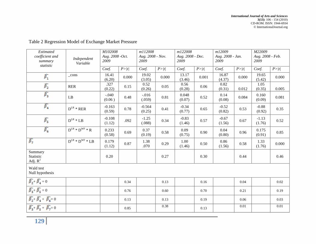
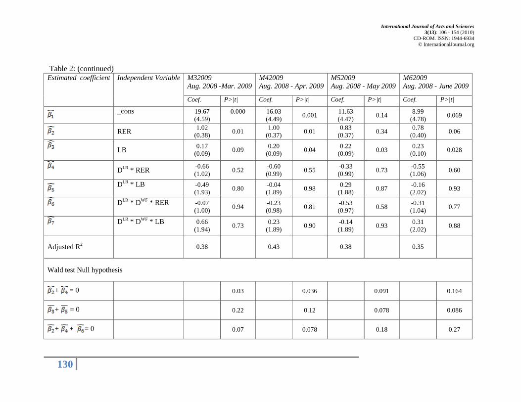
Regression results from estimation of our model (equation 16) for the 40 country sample for each month from October 2008 to June 2009 are presented in Table 2. According to the results of our model (Table 2), movements in the real exchange rate and the lending boom with the interaction effects explain between 20 and 46 percent of the variation in the crisis index. The lowest value of R2 is during the first three months of the crisis (October, November, December 2008) when the volatility and the value of the index were highest (Appendix 3). The regression coefficients in the regression have unexpected signs. The effect of the RER on exchange market pressure for countries with high reserves and strong fundamentals (β2), strong fundamentals and low reserves (β2 + β4) and weak fundamentals and low reserves (β2 + β4 + β6) enter the regression with positive sign, which contradict our theoretical predictions. The coefficient on the lending boom variable has the expected positive sign for countries with high reserves and strong fundamentals (β3) for two months and for countries with weak fundamentals and low reserves (β3 + β5 + β7) in all months. However, an unexpected, negative sign was found for the lending boom estimator of beta for countries with strong fundamentals and low reserves (β3 + β5). Obtained results do not fully support the idea that only countries with overvalued real exchange rates, an insufficient amount of foreign reserves and a lending boom suffer from speculative attack or self-fulfilling panic. Firstly, the estimates of the effect of the lending boom on index of foreign exchange market pressure are statistically insignificant for the first three months after the beginning of the crisis both for countries with low reserves and weak fundamentals and for countries with strong fundamentals but low reserves. Almost the same result is found for effect of the real exchange rate on EMP index. For the time period starting from January 2009 the influence of lending boom and overappriciated real exchange rate was different. The hypothesis that only countries with weak fundamentals are hit by the contagion effect is confirmed for the lending boom variable and not for the real exchange rate. The Wald tests show that (β3 + β5 + β7) referring to influence of lending boom is statistically different from zero for the first five months of 2009 and (β3 + β5) are not significantly different from zero for January, February, March and April. This conclusion is consistent with the results obtained in the benchmark research, Sachs et al. Estimates (β2 + β4 + β6) related to influence of misalignment of real exchange rate is statistically different from zero for the first three months of 2009. However, the estimates of (β2 + β4) are also statistically significant for the first five month of 2009; and we did not expect this result. Furthermore, we found that the RER and LB have important effects on exchange market pressure for eight consecutive months starting from November 2008 for the real exchange rate and for six months starting from January 2009 for Lending boom (Table 3) for countries with strong

International Journal of Arts and Sciences 3(13): 106 - 154 (2010)
CD-ROM. ISSN: 1944-6934 © InternationalJournal.org
128
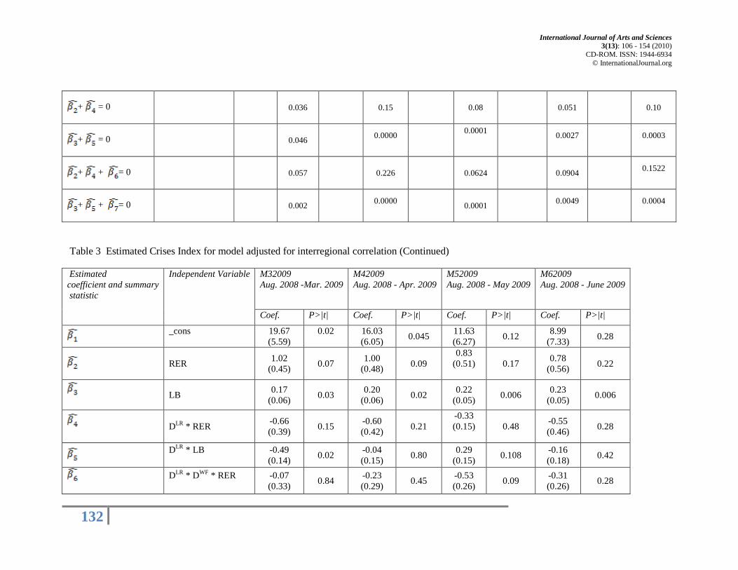
macroeconomic fundamentals and high reserves. Hence it follows that the real exchange rate (RER) and lending boom (LB) variables affect the likelihood of speculative attack in countries both with previously accumulated macroeconomic misbalances and a high level of reserves but weak fundamentals. The hypothesis that only countries with weak fundamentals are vulnerable to shocks is not supported by our results. The dynamics of change in EMP are shown in Figures 1 - 6 in Appendix 3; we see that foreign exchange market pressure exhibits comovement among countries within three regions: emerging Europe, CIS, and East Asia. To control for interregional correlation in the residual structure of our model, we run our main regression model with robust standard errors that cluster residuals at the region level. The main results of the robust regression are given in Table 3. First, we found that influence of the lending boom on EMP is significant for countries with strong fundamentals and low reserves and countries with weak fundamentals and low reserves for all nine months of the study. The estimates attributed to the influence of RER misalignment provide little empirical evidence that the impact of real exchange rate misalignment on EMP affects only fundamentally weak countries.
As in Sachs et al. (1996) we test several alternative hypotheses regarding the vulnerability of an economy to exogenous shocks such as capital flow reversals. This allowed us to check the robustness of the regression results. We investigated whether the ratio of the current account deficit to GDP and government spending to GDP explain variability of EMP. For this purpose we first add the ratio of current account deficit (CA) to GDP22
22 The ratio CA to GDP is calculated as average value of ratios between 2005 and 2008.
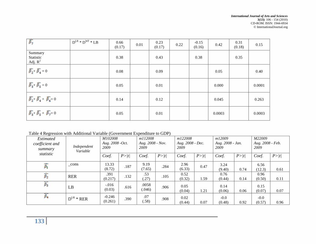
alone and interacted with a dummy variable indicating if the country has low reserves or low reserves and weak fundamentals. Second, we expand our model by adding the average change in the ratio of government expenditures to GDP for 2005-2008. Both regressions provide better explanatory results than the benchmark model. As shown in Table 4 and Table 5, the influence of the current account deficit on the variation of foreign exchange market pressure is statistically significant for four months for the countries with low reserves and strong fundamentals and for 5 months for countries with low reserves and weak fundamentals. The main hypothesis that countries with weak fundamentals are the most vulnerable to the influence of changes in the current account deficit to GDP is not confirmed empirically. We also did not find that countries with weak fundamentals are the only countries in which expansionary fiscal policy significantly affects the foreign exchange market. Coefficient estimates for the ratio of government expenditure to GDP are statistically significant for 6 months for low reserves countries and for 8 months for low reserves/ weak fundamental countries. The main hypothesis of the benchmark model is not supported by the data
International Journal of Arts and Sciences 3(13): 106 - 154 (2010)
CD-ROM. ISSN: 1944-6934 © InternationalJournal.org
129
Table 2 Regression Model of Exchange Market Pressure
Estimated coefficient and
summary statistic
Independent Variable
M102008 Aug. 2008 -Oct. 2009
m112008 Aug. 2008 - Nov. 2009
m122008 Aug. 2008 - Dec. 2009
m12009 Aug. 2008 - Jan. 2009
M22009 Aug. 2008 - Feb. 2009
Coef. P>|t| Coef. P>|t| Coef. P>|t| Coef. P>|t| Coef. P>|t|
_cons
16.41 (6.20) 0.000 19.02
(3.05) 0.000 13.17 (3.46) 0.001 16.87
(4.37) 0.000 19.65 (5.42) 0.000
RER .327 (0.22) 0.15 0.52
(0.26) 0.05 0.56 (0.28) 0.06 0.82
(0.31)
0.012 1.05
(0.35)
0.005
LB -.040 (0.06 ) 0.48 -.016
(.059) 0.81 0.048 (0.07) 0.52 0.14
(0.08) 0.084 0.160 (0.09) 0.081
DLR * RER -0.163 (0.59) 0.78 -0.564
(0.25) 0.41 -0.34 (0.77) 0.65 -0.52
(0.82) 0.53 -0.88 (0.92) 0.35
DLR * LB -0.108 (1.12) .092 -1.25
(.088) 0.34 -0.83 (1.46) 0.57 -0.67
(1.56) 0.67 -1.13 (1.76) 0.52
DLR * DWF * R
0.233 (0.58) 0.69 0.37
(0.19) 0.58 0.09 (0.75) 0.90 0.04
(0.80) 0.96 0.175 (0.91) 0.85
DLR * DWF * LB
0.179 (1.12) 0.87 1.38
.070 0.29 1.00 (1.46) 0.50 0.86
(1.56) 0.58 1.33 (1.76) 0.000
Summary Statistic Adj. R2
0.20 0.27 0.30 0.44
0.46
Wald test Null hypothesis
+ = 0 0.34 0.13 0.16 0.04 0.02
+ = 0 0.76 0.60 0.70 0.21 0.19
+ + = 0 0.13 0.13 0.19 0.06 0.03
+ + = 0 0.85 0.38 0.13 0.01
0.01
International Journal of Arts and Sciences 3(13): 106 - 154 (2010)
CD-ROM. ISSN: 1944-6934 © InternationalJournal.org
130
Table 2: (continued) Estimated coefficient
Independent Variable M32009 Aug. 2008 -Mar. 2009
M42009 Aug. 2008 - Apr. 2009
M52009 Aug. 2008 - May 2009
M62009 Aug. 2008 - June 2009
Coef. P>|t| Coef. P>|t| Coef. P>|t| Coef. P>|t|
_cons
19.67 (4.59)
0.000
16.03 (4.49) 0.001 11.63
(4.47) 0.14 8.99 (4.78) 0.069
RER 1.02 (0.38) 0.01 1.00
(0.37) 0.01 0.83 (0.37) 0.34 0.78
(0.40) 0.06
LB 0.17 (0.09) 0.09 0.20
(0.09) 0.04 0.22 (0.09) 0.03 0.23
(0.10) 0.028
DLR * RER -0.66 (1.02) 0.52 -0.60
(0.99) 0.55 -0.33 (0.99) 0.73 -0.55
(1.06) 0.60
DLR * LB
-0.49 (1.93) 0.80 -0.04
(1.89) 0.98 0.29 (1.88) 0.87 -0.16
(2.02) 0.93
DLR * DWF * RER
-0.07 (1.00) 0.94 -0.23
(0.98) 0.81 -0.53 (0.97) 0.58 -0.31
(1.04) 0.77
DLR * DWF * LB
0.66 (1.94) 0.73 0.23
(1.89) 0.90 -0.14 (1.89) 0.93 0.31
(2.02) 0.88
Adjusted R2 0.38 0.43 0.38 0.35
Wald test Null hypothesis
+ = 0 0.03 0.036 0.091
0.164
+ = 0 0.22 0.12 0.078
0.086
+ + = 0 0.07 0.078 0.18
0.27

International Journal of Arts and Sciences 3(13): 106 - 154 (2010)
CD-ROM. ISSN: 1944-6934 © InternationalJournal.org
131
+ + = 0 0.04 0.008 0.008
0.01
Table 3 Estimated Crises Index for model adjusted for interregional correlation
Estimated coefficient and
summary statistic
Independent Variable
M102008 Aug. 2008 -Oct. 2009
m112008 Aug. 2008 - Nov. 2009
m122008 Aug. 2008 - Dec. 2009
m12009 Aug. 2008 - Jan. 2009
M22009 Aug. 2008 - Feb. 2009
Coef. P>|t| Coef. P>|t| Coef. P>|t| Coef. P>|t| Coef. P>|t|
_cons
16.41 (6.69) 0.001 19.02
(3.59) 0.003 13.17 (3.47) 0.013 16.87
(4.37)
0.012 19.65 (5.42) 0.015
RER
.327 ( .180) 0.13 0.52
(0.22) 0.063 0.56 (0.23) 0.06 0.82
(0.32)
0.049 1.05
(0.39)
0.041
LB
-.040 (.030 ) 0.25
-.016 (.059)
0.799 0.048
(0.034) 0.22 0.14 (0.041)
0.02
0.160 (0.05)
0.032
DLR * RER
-.163 (.199) 0.45 -0.564
(0.25) 0.07 -0.34
(0.198)
0.14 -0.52 (0.30)
0.15
-0.88 (0.35)
0.051
DLR * LB
-.108 (.047) .075
-1.25 (.088)
0.000 -0.83
(0.087) 0.000 -0.671 (0.109)
0.002
-1.126 0.14
0.000
DLR * DWF * R
.233 (.168) 0.22 0.37
(0.19) 0.12 0.09 (0.28) 0.75 0.04
(0.27)
0.891 0.175 (0.30) 0.579
DLR * DWF * LB
.179 (.034) 0.003 1.38
.070 0.000 1.00 (0.18) 0.002 0.86
(0.15)
0.002 1.33
(0.17) 0.000
Summary Statistic Adj. R2
0.20
0.27 0.30 0.44
0.46
Wald test Null hypothesis
International Journal of Arts and Sciences 3(13): 106 - 154 (2010)
CD-ROM. ISSN: 1944-6934 © InternationalJournal.org
132
+ = 0
0.036 0.15 0.08
0.051 0.10
+ = 0
0.046 0.0000
0.0001
0.0027
0.0003
+ + = 0
0.057 0.226 0.0624
0.0904 0.1522
+ + = 0
0.002 0.0000 0.0001
0.0049
0.0004
Table 3 Estimated Crises Index for model adjusted for interregional correlation (Continued)
Estimated coefficient and summary statistic
Independent Variable M32009 Aug. 2008 -Mar. 2009
M42009 Aug. 2008 - Apr. 2009
M52009 Aug. 2008 - May 2009
M62009 Aug. 2008 - June 2009
Coef. P>|t| Coef. P>|t| Coef. P>|t| Coef. P>|t|
_cons
19.67 (5.59)
0.02
16.03 (6.05) 0.045 11.63
(6.27) 0.12 8.99 (7.33) 0.28
RER 1.02 (0.45) 0.07 1.00
(0.48) 0.09 0.83
(0.51)
0.17 0.78 (0.56) 0.22
LB 0.17 (0.06) 0.03 0.20
(0.06) 0.02 0.22 (0.05) 0.006 0.23
(0.05) 0.006
DLR * RER -0.66 (0.39) 0.15 -0.60
(0.42) 0.21 -0.33 (0.15)
0.48 -0.55
(0.46) 0.28
DLR * LB
-0.49 (0.14) 0.02 -0.04
(0.15) 0.80 0.29 (0.15) 0.108 -0.16
(0.18) 0.42
DLR * DWF * RER
-0.07 (0.33) 0.84 -0.23
(0.29) 0.45 -0.53 (0.26) 0.09 -0.31
(0.26) 0.28
International Journal of Arts and Sciences 3(13): 106 - 154 (2010)
CD-ROM. ISSN: 1944-6934 © InternationalJournal.org
133
DLR * DWF * LB
0.66 (0.17) 0.01 0.23
(0.17) 0.22 -0.15 (0.16) 0.42 0.31
(0.18) 0.15
Summary Statistic Adj. R2
0.38 0.43 0.38 0.35
+ = 0 0.08 0.09 0.05
0.40
+ = 0 0.05 0.01 0.000
0.0001
+ + = 0 0.14 0.12 0.045
0.263
+ + = 0 0.05 0.01 0.0003
0.0003
Table 4 Regression with Additional Variable (Government Expenditure to GDP) Estimated
coefficient and summary statistic
Independent Variable
M102008 Aug. 2008 -Oct. 2009
m112008 Aug. 2008 - Nov. 2009
m122008 Aug. 2008 - Dec. 2009
m12009 Aug. 2008 - Jan. 2009
M22009 Aug. 2008 - Feb. 2009
Coef. P>|t| Coef. P>|t| Coef. P>|t| Coef. P>|t| Coef. P>|t|
_cons
13.33 (8.72) .187 9.19
(7.65) .284 2.96 (6.33) 0.47 3.24
(9.40) 0.74 6.56
(12.3) 0.61
RER .391 (0.217) .132 .53
(.27) .105 0.52 (0.32) 1.59
0.76 (0.44) 0.14
0.96 (0.50) 0.11
LB -.016 (0.03) .616 .0058
(.046) .906 0.05 (0.04) 1.21
0.14 (0.06) 0.06
0.15 (0.07) 0.07
DLR * RER -0.246 (0.261) .390 .07
(.58) .908 0.02 (0.44) 0.07
-0.0 (0.48) 0.92
-0.0 (0.57) 0.96
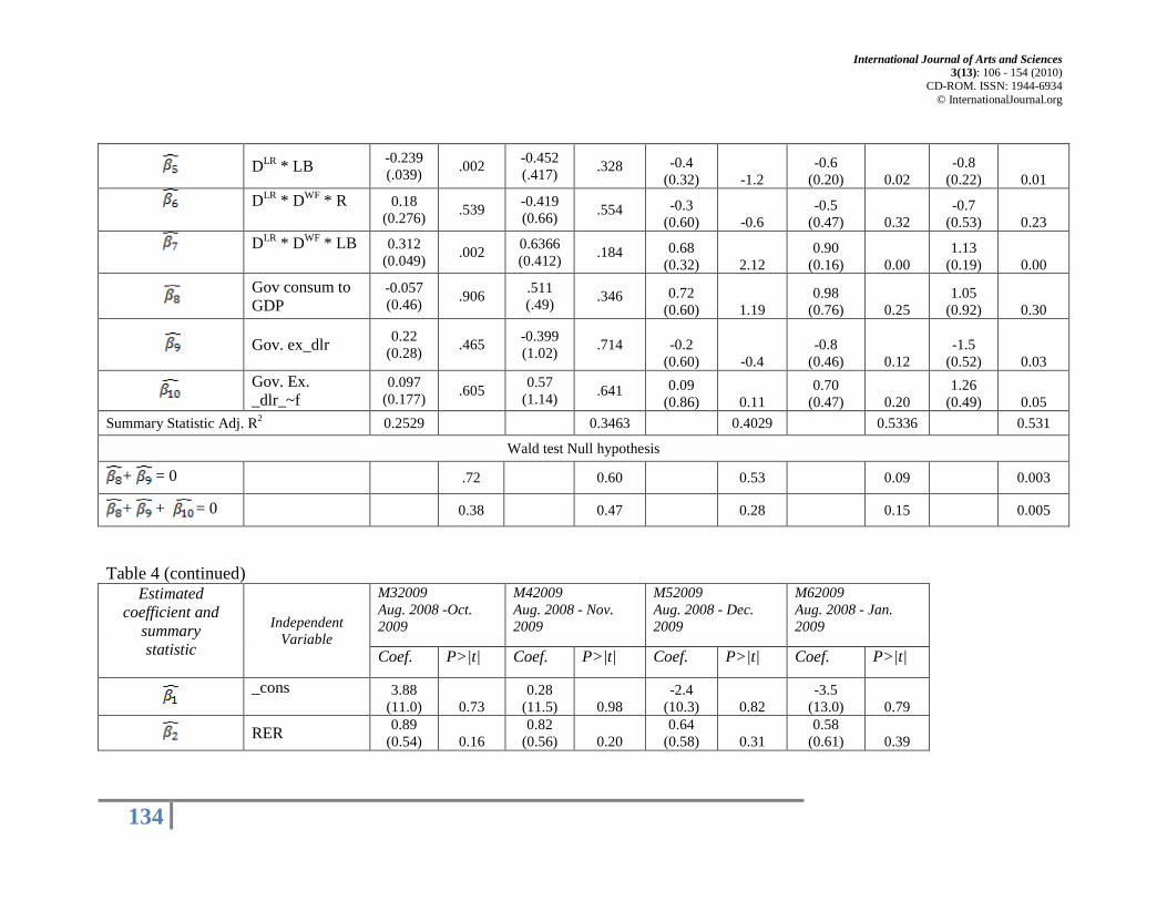
International Journal of Arts and Sciences 3(13): 106 - 154 (2010)
CD-ROM. ISSN: 1944-6934 © InternationalJournal.org
134
DLR * LB -0.239 (.039) .002 -0.452
(.417) .328 -0.4 (0.32) -1.2
-0.6 (0.20) 0.02
-0.8 (0.22) 0.01
DLR * DWF * R
0.18 (0.276) .539 -0.419
(0.66) .554 -0.3 (0.60) -0.6
-0.5 (0.47) 0.32
-0.7 (0.53) 0.23
DLR * DWF * LB
0.312 (0.049) .002 0.6366
(0.412) .184 0.68 (0.32) 2.12
0.90 (0.16) 0.00
1.13 (0.19) 0.00
Gov consum to GDP
-0.057 (0.46) .906 .511
(.49) .346 0.72 (0.60) 1.19
0.98 (0.76) 0.25
1.05 (0.92) 0.30
Gov. ex_dlr 0.22 (0.28) .465 -0.399
(1.02) .714 -0.2 (0.60) -0.4
-0.8 (0.46) 0.12
-1.5 (0.52) 0.03
Gov. Ex. _dlr_~f
0.097 (0.177) .605 0.57
(1.14) .641 0.09 (0.86) 0.11
0.70 (0.47) 0.20
1.26 (0.49) 0.05
Summary Statistic Adj. R2 0.2529 0.3463 0.4029 0.5336 0.531
Wald test Null hypothesis
+ = 0 .72 0.60 0.53 0.09 0.003
+ + = 0 0.38 0.47 0.28 0.15 0.005
Table 4 (continued) Estimated
coefficient and summary statistic
Independent Variable
M32009 Aug. 2008 -Oct. 2009
M42009 Aug. 2008 - Nov. 2009
M52009 Aug. 2008 - Dec. 2009
M62009 Aug. 2008 - Jan. 2009
Coef. P>|t| Coef. P>|t| Coef. P>|t| Coef. P>|t|
_cons
3.88 (11.0) 0.73
0.28 (11.5) 0.98
-2.4 (10.3) 0.82
-3.5 (13.0) 0.79
RER 0.89 (0.54) 0.16
0.82 (0.56) 0.20
0.64 (0.58) 0.31
0.58 (0.61) 0.39
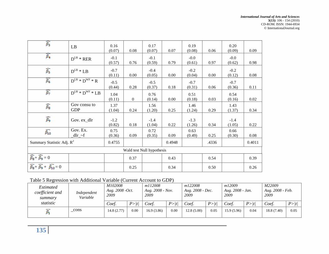
International Journal of Arts and Sciences 3(13): 106 - 154 (2010)
CD-ROM. ISSN: 1944-6934 © InternationalJournal.org
135
LB 0.16 (0.07) 0.08
0.17 (0.07) 0.07
0.19 (0.08) 0.06
0.20 (0.09) 0.09
DLR * RER -0.1 (0.57) 0.76
-0.1 (0.59) 0.79
-0.0 (0.61) 0.97
-0.0 (0.62) 0.98
DLR * LB -0.7 (0.11) 0.00
-0.4 (0.05) 0.00
-0.2 (0.04) 0.00
-0.2 (0.12) 0.08
DLR * DWF * R
-0.5 (0.44) 0.28
-0.5 (0.37) 0.18
-0.7 (0.31) 0.06
-0.7 (0.36) 0.11
DLR * DWF * LB
1.04 (0.11) 0
0.76 (0.14) 0.00
0.51 (0.18) 0.03
0.54 (0.16) 0.02
Gov consu to GDP
1.37 (1.04) 0.24
1.56 (1.20) 0.25
1.46 (1.24) 0.29
1.43 (1.37) 0.34
Gov. ex_dlr -1.2 (0.82) 0.18
-1.4 (1.04) 0.22
-1.3 (1.26) 0.34
-1.4 (1.05) 0.22
Gov. Ex. _dlr_~f
0.75 (0.36) 0.09
0.72 (0.35) 0.09
0.63 (0.49) 0.25
0.66 (0.30) 0.08
Summary Statistic Adj. R2 0.4755 0.4948 .4336 0.4011
Wald test Null hypothesis
+ = 0 0.37 0.43 0.54 0.39
+ + = 0 0.25 0.34 0.50 0.26
Table 5 Regression with Additional Variable (Current Account to GDP)
Estimated coefficient and
summary statistic
Independent Variable
M102008 Aug. 2008 -Oct. 2009
m112008 Aug. 2008 - Nov. 2009
m122008 Aug. 2008 - Dec. 2009
m12009 Aug. 2008 - Jan. 2009
M22009 Aug. 2008 - Feb. 2009
Coef. P>|t| Coef. P>|t| Coef. P>|t| Coef. P>|t| Coef. P>|t|
_cons
14.8 (2.77) 0.00 16.9 (3.86) 0.00 12.8 (5.00) 0.05 15.9 (5.96) 0.04 18.8 (7.40) 0.05

International Journal of Arts and Sciences 3(13): 106 - 154 (2010)
CD-ROM. ISSN: 1944-6934 © InternationalJournal.org
136
RER 0.29 (0.18) 0.16 0.47 (0.22) 0.08 0.55 (0.25) 0.07 0.80 (0.36) 0.07 1.05 (0.46) 0.07
LB -0.0 (0.02) 0.28 0.00 (0.04) 0.91 0.05 (0.04) 0.26 0.14 (0.05) 0.03 0.16 (0.06) 0.05
DLR * RER -0.1 (0.15) 0.36 0.09 (0.22) 0.68 -0.0 (0.24) 0.82 -0.3 (0.32) 0.33 -0.4 (0.40) 0.28
DLR * LB -0.2 (0.04) 0.00 -0.5 (0.12) 0.00 -0.4 (0.13) 0.01 -0.5 (0.11) 0.00 -0.6 (0.13) 0.00
DLR * DWF * R 0.23 (0.15) 0.17 -0.3 (0.18) 0.16 -0.2 (0.25) 0.30 -0.2 (0.25) 0.46 -0.3 (0.27) 0.31
DLR * DWF * LB 0.31 (0.09) 0.02 0.72 (0.17) 0.00 0.83 (0.16) 0.00 0.86 (0.13) 0.00 1.02 (0.14) 0.00
CA *DLR -0.2 (0.20) 0.29 -0.3 (0.24) 0.20 -0.0 (0.26) 0.80 -0.1 (0.33) 0.73 -0.0 (0.38) 0.91
CA_gdp_dlr 0.01 (0.24) 0.96 2.05 (0.44) 0.00 0.81 (0.30) 0.04 0.80 (0.47) 0.15 1.77 (0.62) 0.03
Ca_gdp_dlr_dwf 0.08 (0.60) 0.89 -1.6 (0.78) 0.08 0.33 (0.56) 0.57 0.15 (0.53) 0.78 -0.9 (0.65) 0.22
Summary Statistic Adj. R2 0.2496 0.3387 0.4698 0.5398 0.5328 Wald test Null hypothesis
+ = 0 .01 0.01 0.05 0.17 0.04
+ + = 0 0.03 0.02 0.03 0.17 0.06
Table 5 (continued) Estimated
coefficient and summary statistic
Independent Variable
M32009 Aug. 2008 -Oct. 2009
M42009 Aug. 2008 - Nov. 2009
M52009 Aug. 2008 - Dec. 2009
M62009 Aug. 2008 - Jan. 2009
Coef. P>|t| Coef. P>|t| Coef. P>|t| Coef. P>|t|
_cons
19.0 (7.93) 0.06 15.7 (7.96) 0.10 12.2 (8.08) 0.18 10.1 (9.35) 0.32

International Journal of Arts and Sciences 3(13): 106 - 154 (2010)
CD-ROM. ISSN: 1944-6934 © InternationalJournal.org
137
RER 1.02 (0.51) 0.10 0.97 (0.54) 0.12 0.82 (0.54) 0.19 0.79 (0.57) 0.22
LB 0.17 (0.07) 0.05 0.20 (0.06) 0.02 0.21 (0.06) 0.02 0.22 (0.07) 0.02
DLR * RER -0.6 (0.42) 0.17 -0.7 (0.43) 0.16 -0.5 (0.42) 0.22 -0.5 (0.45) 0.25
DLR * LB -0.5 (0.13) 0.00 -0.2 (0.14) 0.13 -0.0 (0.13) 0.79 -0.1 (0.16) 0.51
DLR * DWF * R
-0.1 (0.27) 0.62 -0.1 (0.24) 0.56 -0.3 (0.25) 0.27 -0.3 (0.23) 0.19
DLR * DWF * LB 0.92 (0.14) 0.00 0.59 (0.16) 0.01 0.32 (0.17) 0.11 0.41 (0.17) 0.06
ca_gdp -0.0 (0.30) 0.93 -0.1 (0.30) 0.67 0.03 (0.28) 0.89 0.15 (0.29) 0.61
Ca_gdp_dlr 0.33 (0.71) 0.65 0.14 (0.83) 0.86 -0.3 (0.93) 0.71 0.33 (0.73) 0.66
Ca_gdp_dlr_dwf 0.71 (0.78) 0.40 0.89 (0.92) 0.37 1.27 (0.93) 0.22 0.57 (0.68) 0.44
Summary Statistic Adj. R2 0.47 0.47 0.42 0.4016
Wald test Null hypothesis
+ = 0 0.88 0.90 0.92 0.63
+ + = 0 0.44 0.51 0.41 0.35

International Journal of Arts and Sciences 3(13): 106 - 154 (2010)
CD-ROM. ISSN: 1944-6934 © InternationalJournal.org
138
6. CONCLUSIONS During the global financial crises many developing countries that were not at the epicenter of the crisis experienced sharp depreciation of their currencies. Our research evaluated the role played by macroeconomic fundamentals in generating pressure on foreign exchange markets. Using data on 40 developing countries we estimated the effect of domestic credit expansion, misalignment of the real exchange rate, changes in the ratio of the current account to GDP and changes in the ratio of government expenditure to GDP on the index of foreign exchange market pressure from October 2008 to June 2009.
We found empirical evidence that lending boom and overvalued real exchange, ratio of the current account deficit to GDP and government expenditure to GDP partially explain the movement in foreign exchange market pressure. However, the explanatory power of the model was the lowest when the it was applied to the months of the highest exchange market disturbances (October, November 2008). For the first three months after September 2008 the effects of the lending boom and the real exchange rate on exchange market pressure were not significant for both countries with weak and strong macroeconomic fundamentals. This implies that, during the most severe stage of the crisis, instabilities in foreign exchange markets were triggered more by other “market driven” factors such as flight-to-haven flows, interest rate differentials, and global liquidity conditions than by accumulated macroeconomic misbalances.
Our data do not support the hypothesis that fundamental macroeconomic indifferences explain the magnitude and depth of financial market disturbances. Weak banking system and overappriciated real exchange rate are positively related to the size of foreign exchange market pressure aroused during the global financial crises both for countries with strong and weak fundamentals. This supports the insights of the “second generation” of currency crisis models. Foreign exchange market disturbances were to some extent unresponsive to underlying macroeconomic variables. This result has important implications for policymaking. Currently national economic policies alone, even if successful, might not be sufficient to prevent instability in the foreign exchange market, but policies that strengthen the global institutional infrastructure to curb highly volatile capital flows can have more impact.
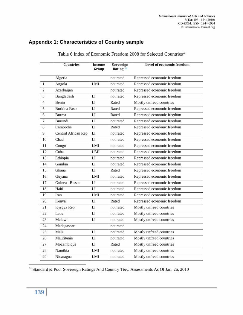
International Journal of Arts and Sciences 3(13): 106 - 154 (2010)
CD-ROM. ISSN: 1944-6934 © InternationalJournal.org
139
Appendix 1: Characteristics of Country sample
Table 6 Index of Economic Freedom 2008 for Selected Countries*
Countries Income Group
Sovereign Rating 23
Level of economic freedom
Algeria not rated Repressed economic freedom 1 Angola LMI not rated Repressed economic freedom 2 Azerbaijan not rated Repressed economic freedom 3 Bangladesh LI not rated Repressed economic freedom 4 Benin LI Rated Mostly unfreed countries 5 Burkina Faso LI Rated Repressed economic freedom 6 Burma LI Rated Repressed economic freedom 7 Burundi LI not rated Repressed economic freedom 8 Cambodia LI Rated Repressed economic freedom 9 Central African Rep LI not rated Repressed economic freedom 10 Chad LI not rated Repressed economic freedom 11 Congo LMI not rated Repressed economic freedom 12 Cuba UMI not rated Repressed economic freedom 13 Ethiopia LI not rated Repressed economic freedom 14 Gambia LI not rated Repressed economic freedom 15 Ghana LI Rated Repressed economic freedom 16 Guyana LMI not rated Repressed economic freedom 17 Guinea –Bissau LI not rated Repressed economic freedom 18 Haiti LI not rated Repressed economic freedom 19 Iran LMI not rated Repressed economic freedom 20 Kenya LI Rated Repressed economic freedom 21 Kyrgyz Rep LI not rated Mostly unfreed countries 22 Laos LI not rated Mostly unfreed countries 23 Malawi LI not rated Mostly unfreed countries 24 Madagascar not rated 25 Mali LI not rated Mostly unfreed countries 26 Mauritania LI not rated Mostly unfreed countries 27 Mozambique LI Rated Mostly unfreed countries 28 Namibia LMI not rated Mostly unfreed countries 29 Nicaragua LMI not rated Mostly unfreed countries
23 Standard & Poor Sovereign Ratings And Country T&C Assessments As Of Jan. 26, 2010

International Journal of Arts and Sciences 3(13): 106 - 154 (2010)
CD-ROM. ISSN: 1944-6934 © InternationalJournal.org
140
30 Nepal LI not rated Mostly unfreed countries 31 Nigeria LI Rated Mostly unfreed countries 32 Pakistan LI Rated Mostly unfreed countries 33 Rwanda LI not rated Mostly unfreed countries 34 Senegal LI Rated Mostly unfreed countries 35 Syria LMI not rated Repressed economic freedom 36 Sierra Leone LI not rated Mostly unfreed countries 37 Swaziland LMI not rated Mostly unfreed countries 38 Tanzania LI not rated Mostly unfreed countries 39 Togo LI not rated Mostly unfreed countries 40 Uzbekistan LI not rated Mostly unfreed countries 41 Vietnam LI Rated Mostly unfreed countries 42 Yemen LI not rated Mostly unfreed countries 43 Zambia LI not rated Mostly unfreed countries 44 Zimbabwe LI not rated Mostly unfreed countries
* 2008 Index of Economic Freedom: WSJ, Heritage Foundation
Table 7 Domestic credit to private sector to GDP and Total Volume of Stock Traded to GDP in
Low Income Countries in 2008
Country Name Domestic credit to private sector (% of GDP)
Stocks traded, total value (% of GDP)
1 Afghanistan .. .. 2 Bangladesh 39.49 11.70 3 Benin 20.87 .. 4 Burkina Faso 18.61 .. 5 Burundi 21.48 .. 6 Cambodia 23.46 .. 7 Central African Republic 7.03 .. 8 Chad 3.74 .. 9 Comoros 11.49 .. 10 Congo, Dem. Rep. .. .. 11 Cote d'Ivoire 16.25 1.35 12 Eritrea .. .. 13 Ethiopia .. .. 14 Gambia, The .. ..

International Journal of Arts and Sciences 3(13): 106 - 154 (2010)
CD-ROM. ISSN: 1944-6934 © InternationalJournal.org
141
15 Ghana .. 0.93 16 Guinea .. .. 17 Guinea-Bissau 9.06 .. 18 Haiti .. .. 19 Kenya 26.40 4.17 20 Korea, Dem. Rep. .. .. 21 Kyrgyz Republic .. 2.54 22 Lao PDR .. .. 23 Liberia .. .. 24 Madagascar 11.14 .. 25 Malawi .. 1.40 26 Mali 17.15 .. 27 Mauritania .. .. 28 Mozambique 18.73 .. 29 Myanmar .. .. 30 Nepal 40.80 2.90 31 Niger 10.95 .. 32 Nigeria 33.11 9.41 33 Pakistan .. 32.30 34 Papua New Guinea 25.65 .. 35 Rwanda .. .. 36 Sao Tome and Principe 28.30 .. 37 Senegal 24.19 .. 38 Sierra Leone 7.10 .. 39 Solomon Islands 30.49 .. 40 Somalia .. .. 41 Tajikistan .. .. 42 Tanzania 16.25 .. 43 Togo 19.24 .. 44 Uganda 14.11 .. 45 Uzbekistan .. 0.30 46 Vietnam 90.57 4.63 47 Yemen, Rep. 7.80 .. 48 Zambia 15.30 .. 49 Zimbabwe .. .. Mean value 22.55 6.51

International Journal of Arts and Sciences 3(13): 106 - 154 (2010)
CD-ROM. ISSN: 1944-6934 © InternationalJournal.org
142
Table 8 Domestic credit to private sector to GDP and Total Volume of Stock Traded to GDP in Lower Middle Income Countries in 2008
Country Domestic credit to private sector (% of GDP)
Stocks traded, total value (% of GDP)
1 Albania 36 0.00 2 Algeria 13 0 3 Angola 13 0 4 Armenia 17 0 5 Bolivia 35 0 6 Bosnia and
Herzegovina 58 0
7 Cameroon 10 0 8 Cape Verde 54 0 9 China 108 126 10 Colombia 34 5 11 Congo, Rep. 3 0 12 Djibouti 28 0 13 Dominican
Republic 21 0
14 Ecuador 27 0 15 Egypt, Arab Rep. 43 43 16 Georgia 33 0 17 Guatemala 27 0 18 Guyana 57 0 19 Honduras 51 0 20 India 50 86 21 Indonesia 27 22 22 Jordan 89 140 23 Lesotho 11 0 24 Macedonia, FYR 44 2 25 Mongolia 44 1 26 Morocco 80 25 27 Namibia 47 0 28 Paraguay 24 0 29 Philippines 29 20 30 Sri Lanka 29 3 31 Moldova 37 3 32 Sudan 11 0

International Journal of Arts and Sciences 3(13): 106 - 154 (2010)
CD-ROM. ISSN: 1944-6934 © InternationalJournal.org
143
33 Suriname 28 0 34 Syrian Arab
Republic 16 0
35 Tonga 0 0 36 Tunisia 67 4 37 Turkmenistan 0 0 38 Ukraine 74 1 39 Vanuatu 57 0 Mean 36.72 12.33
Table 9 Domestic credit to private sector to GDP and Total Volume of Stock Traded to GDP in Upper Middle Income Countries in 2008
Country Name Domestic credit to
private sector (% of GDP)
Stocks traded, total value (% of
GDP)
1 Algeria 12.94 ..
2 American Samoa .. ..
3 Belarus 28.84 ..
4 Bosnia and Herzegovina
57.98 ..
5 Dominica 61.56 ..
6 Dominican Republic 21.17 ..
7 Gabon 8.61 ..
8 Grenada 90.70 ..
9 Mayotte .. ..
10 Palau .. ..
11 Seychelles 38.34 ..
12 Suriname 27.53 ..
13 Uruguay 26.51 ..
14 Venezuela, RB 21.52 ..
15 South Africa 79.55 145.07
16 Thailand 39.35 118.21
17 Malaysia 100.57 43.72
18 Russian Federation 42.01 34.97

International Journal of Arts and Sciences 3(13): 106 - 154 (2010)
CD-ROM. ISSN: 1944-6934 © InternationalJournal.org
144
19 Chile 84.95 21.57
20 China 108.31 126.45
21 Montenegro 80.59 2.33
22 Jamaica 28.32 2.40
23 Peru 25.09 4.01
24 Mauritius 93.55 4.66
25 Croatia 64.94 4.96
26 Brazil 55.71 45.13
27 Colombia 34.38 5.15
28 Lebanon 77.50 2.46
29 Panama 89.75 1.11
30 Botswana 21.96 1.11
31 Serbia 38.40 2.49
32 Kazakhstan 50.10 2.61
33 Bulgaria 74.49 3.31
34 Poland 49.86 12.90
35 Fiji 48.18 0.08
36 Argentina 13.63 4.09
37 Turkey 31.62 30.18
38 Macedonia, FYR 43.81 1.64
39 Lithuania 62.71 1.03
40 Namibia 47.08 0.22
41 Costa Rica 50.48 ..
42 Latvia 90.19 0.12
mean 53.23 22.21
Table 10 Total Value of Stock Traded, Market capitalization and Net Domestic Credit for Upper Middle Income Countries (annual volume, 2008)*
Country Name Stocks traded, total
value (current US$) Market capitalization of listed companies (current US$)
Net domestic credit (current LCU)
1 China 5,470,529,157,182.00 2,793,612,600,029.31 37,937,867,000,000.00 2 Brazil 727,792,742,692.10 589,384,021,012.01 2,922,966,944,112.39 3 Russian Federation 562,229,865,850.82 1,321,832,550,000.00 10,787,800,000,000.00

International Journal of Arts and Sciences 3(13): 106 - 154 (2010)
CD-ROM. ISSN: 1944-6934 © InternationalJournal.org
145
4 South Africa 401,493,248,703.07 491,281,773,931.86 2,000,011,642,565.60 5 Turkey 239,713,337,154.69 117,929,860,382.25 499,430,792,902.35 6 Malaysia 85,213,924,007.09 187,065,751,445.09 853,476,966,720.14 7 Poland 67,954,587,588.92 90,232,639,217.01 764,415,000,000.00 8 Chile 36,558,776,599.35 132,428,480,313.85 73,247,264,280,000.00 9 Argentina 13,419,755,720.77 52,309,391,298.05 246,508,929,000.00 10 Colombia 12,483,673,243.46 87,032,363,669.52 197,149,826,638,539.00 11 Peru 5,111,322,952.86 55,625,279,630.51 69,015,222,625.00 12 Kazakhstan 3,446,784,063.81 31,075,188,293.69 5,379,083,350,627.46 13 Croatia 3,440,006,207.91 26,790,141,150.51 256,936,992,200.42 14 Bulgaria 1,650,692,438.59 8,857,549,047.48 44,531,000,000.00 15 Serbia 1,248,492,700.00 12,165,130,600.00 1,073,068,400,000.00 16 Lebanon 705,306,039.69 9,640,557,823.16 76,283,212,502,079.70 17 Lithuania 489,127,563.36 3,624,948,108.29 71,574,000,000.00 18 Mauritius 403,240,996.73 3,442,532,576.38 296,097,984,659.89 19 Jamaica 361,851,412.96 7,512,918,694.34 575,593,154,000.00 20 Panama 256,131,796.75 6,567,868,000.00 19,800,675,592.33 21 Macedonia, FYR 156,074,664.86 823,485,800.00 170,142,898,157.50 22 Botswana 144,169,283.19 3,555,774,353.05 -10,233,132,574.00 23 Montenegro 105,179,600.00 2,862,593,600.00 2,702,184,203.04 24 Latvia 42,178,738.70 1,608,811,696.60 14,478,000,000.00 25 Namibia 18,764,965.14 618,688,184.10 31,930,251,589.05 26 Fiji 2,889,701.62 568,223,337.57 3,166,439,314.62 27 Algeria .. .. -1,402,359,013,553.10 28 Belarus .. .. 40,524,116,200,000.00 29 Costa Rica .. 1,887,039,730.19 8,415,600,927,480.23 30 Dominican Republic .. .. 619,186,640,181.00 31 Gabon .. .. 394,843,000,000.00 32 Uruguay .. .. 223,555,211,288.94 33 Venezuela, RB .. .. 134,232,169,599.85 34 Bosnia and
Herzegovina .. .. 14,456,639,810.00
35 Seychelles .. .. 6,224,517,201.10 36 Suriname .. .. 2,181,134,852.62 37 Grenada .. .. 1,776,498,620.00 38 Dominica .. .. 564,221,387.00 39 American Samoa .. .. .. 40 Mayotte .. .. .. 41 Palau .. .. ..
* Sourse of Data: World Development Indicators, World Bank, IMF.

International Journal of Arts and Sciences 3(13): 106 - 154 (2010)
CD-ROM. ISSN: 1944-6934 © InternationalJournal.org
146
Table 11 List of Countries in the Sample
Country Name Domestic credit
to private sector (% of GDP)
Stocks traded, total value (% of
GDP)
1 Argentina 13.63 4.09 2 Albania 36.00 0.00 3 Bangladesh 39.49 11.70 4 Brazil 55.71 45.13 5 Bulgaria 74.49 3.31 6 Bosnia and Herzegovina 58.00 0.00 7 Chile 84.95 21.57 8 China 108.31 126.45 9 Colombia 34.38 5.15
10 Croatia 64.94 4.96 11 Czech Republic 52.53 19.88 12 Egypt, Arab Rep. 43.00 43.00 13 Estonia 98.68 3.39 14 Hungary 69.60 20.00 15 India 50.00 86.00 16 Indonesia 27.00 22.00 17 Jordan 89.00 140.00 18 Kazakhstan 50.10 2.61 19 Kenya 26.40 4.17 20 Latvia 90.19 0.12 21 Lebanon 77.50 2.46 22 Lithuania 62.71 1.03 23 Malaysia 100.57 43.72 24 Macedonia, FYR 44.00 2.00 25 Mexico 21.10 10.00 26 Moldova 37.00 3.00 27 Mongolia 44.00 1.00 28 Morocco 80.00 25.00 29 Nigeria 33.11 9.41 30 Pakistan .. 32.30 31 Peru 25.09 4.01 32 Poland 49.86 12.90
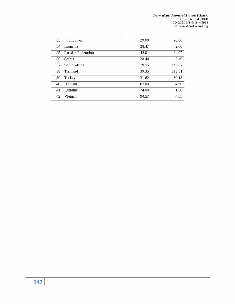
International Journal of Arts and Sciences 3(13): 106 - 154 (2010)
CD-ROM. ISSN: 1944-6934 © InternationalJournal.org
147
33 Philippines 29.00 20.00 34 Romania 38.47 2.00 35 Russian Federation 42.01 34.97 36 Serbia 38.40 2.49 37 South Africa 79.55 145.07 38 Thailand 39.35 118.21 39 Turkey 31.62 30.18 40 Tunisia 67.00 4.00 41 Ukraine 74.00 1.00 42 Vietnam 90.57 4.63

International Journal of Arts and Sciences 3(13): 106 - 154 (2010)
CD-ROM. ISSN: 1944-6934 © InternationalJournal.org
148
Appendix 2: Explanatory and Dependent Variables for Countries in Sample
Table 12. Explanatory Variables for Countries in the Sample and Index of Foreign Exchange Pressure for October 2008
Country IND24 RER 25 LB 26 M2/R 27
1
ARGENTINA 11.51 -23.88 -36.51 1.24
2 BANGLADESH 6.94 -8.09 9.07 6.33
3 BOSNIA-HERZEGOVINA 31.65 0.79 33.12 2.57
4 BRAZIL 38.55 42.65 36.52 2.89
5 BULGARIA 27.13 17.63 56.07 1.74
6 CHILE 16.93 9.94 -1.07 4.29
7 CHINA -0.6 20.51 13.47 3.47
8 COLOMBIA 26.41 9.74 16.91 3.48
9 CROATIA 26.60 20.18 32.7 3.29
10 CZECH REPUBLIC 24.11 -7.7 -25.75 3.95
11 EGYPT 3.41 11.85 43.18 4.45
12 ESTONIA 12.65 15.85 29.45 2.80
13 HUNGARY 33.72 4.63 16.84 3.32
14 INDIA 28.02 26.75 -20.51 3.28
15 INDONESIA 23.88 -16.24 11.32 3.26
16 JORDAN -2.79 17.41 36.67 3.04
17 KAZAKHSTAN 2.96 36.14 -8.02 1.73
18 KENYA 23.56 4.36 24.02 3.28
19 LATVIA 18.72 -11.58 -1.41 2.24
20 LEBANON -7.68 4.52 48.99 1.18
21 LITHUANIA 16.9 -2.25 113.75 3.00
22 MACEDONIA 19.28 -3.4 -15.42 1.23
23 MALAYSIA 24.31 -8.72 16.69 2.15
24 MEXICO 36.2 14.01 26.3 5.71
25 MOLDOVA 14.44 0.49 28.53 1.28
26 MOROCCO 27.57 -1.97 203.52 3.55
27 NIGERIA 2.75 3.86 3.99 1.18
24 Index of Foreign Exchange Market Pressure is calculated between October 2008 and August 2008 which is as the base month and is given in percentage points. 25 Average percentage change in Real Exchange Rate between between 2001-2004 and between 2005-2008 26 Average percentage change in Ratio of Domestic credit provided by the banking sector to GDP)between 2005 and 2008 27 Broad money (M2) to total reserves minus gold measured in the national currency, August 2008

International Journal of Arts and Sciences 3(13): 106 - 154 (2010)
CD-ROM. ISSN: 1944-6934 © InternationalJournal.org
149
28 PAKISTAN 41.39 -3.13 6.38 8.61
29 PERU 14.98 15.99 -9.22 0.56
30 PHILIPPINES 9.23 10.75 60.9 1.42
31 POLAND 45.14 29.2 97.04 3.56
32 ROMANIA 28.32 34.56 28.48 1.80
33 RUSSIAN FEDERATION 26.27 30.01 36.99 1.06
34 SERBIA 34.12 4.55 -51.78 0.54
35 SOUTH AFRICA 30.51 22.19 8.95 6.19
36 THAILAND -0.43 -11.31 3.12 2.81
37 TUNISIA 18.18 30.03 8.62 2.91
38 TURKEY 32.34 11.24 146.5 4.27
39 UKRAINE 20.45 5.1 33.29 2.60
40 VIETNAM -6.29 0.05 0.33 3.53
MEAN 19.54 8.9 26.36 2.96
STD. DEVIATION 13.4 15 47 1.665
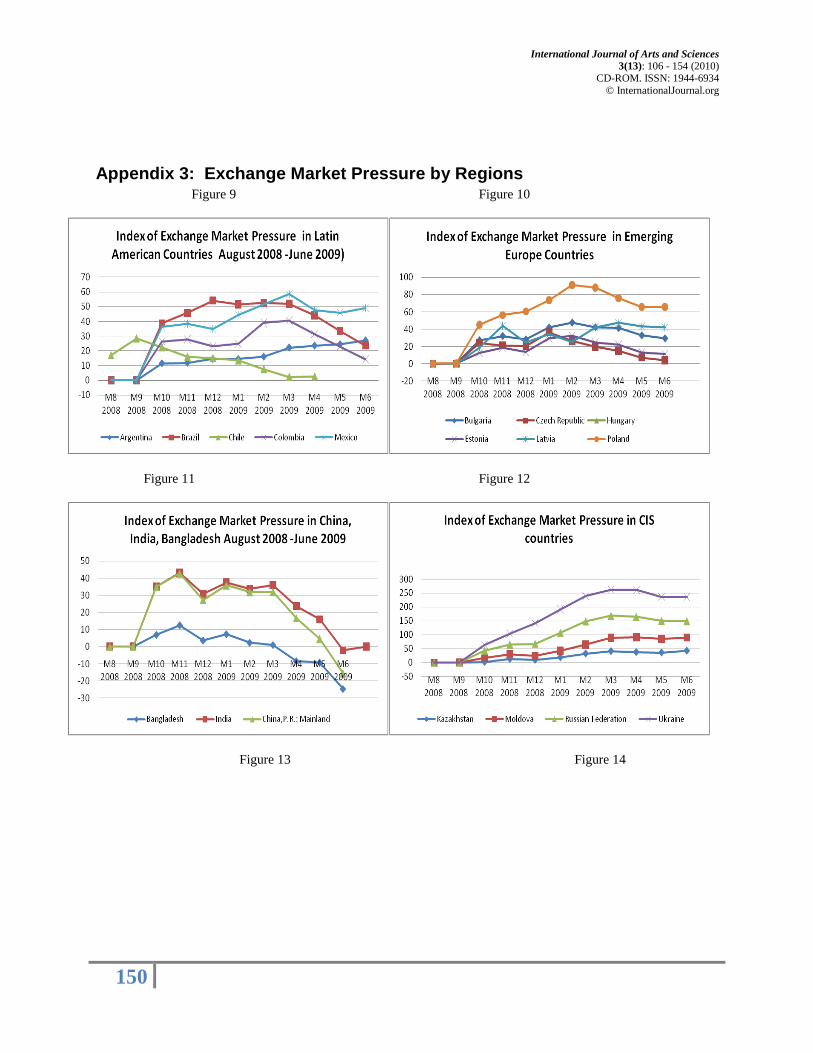
International Journal of Arts and Sciences 3(13): 106 - 154 (2010)
CD-ROM. ISSN: 1944-6934 © InternationalJournal.org
150
Appendix 3: Exchange Market Pressure by Regions Figure 9 Figure 10
Figure 11 Figure 12
Figure 13 Figure 14

International Journal of Arts and Sciences 3(13): 106 - 154 (2010)
CD-ROM. ISSN: 1944-6934 © InternationalJournal.org
151
International Journal of Arts and Sciences 3(13): 106 - 154 (2010)
CD-ROM. ISSN: 1944-6934 © InternationalJournal.org
152
7. BIBLIOGRAPHY
Agenor, P., Bhandari J., Flood R.P. (1992) Speculative Attacks and Model of Balance of Payments Crisis. IMF Staff Papers, 39, 357-394
Berg, A., Pattillo C. (1998) Are Currency Crises Predictable? A Test. IMF Working Paper, (98)154
Blanco H., Garber P. M. (1986) Recurrent Devaluation and Speculative Attack on the Mexican Peso. Journal of Political Economy, 94 (1), 148-166
Blanchard, Oliver (2008) The Crisis: Basic Mechanisms, and Appropriate Policies. Massachusetts Institute of Technology, Department of Economics Working Paper, 09-01
Burnside, C., Eichenbaum M., Rebelo S. (2007) Currency Crisis Models. The New Palgrave: A Dictionary of Economics, 2
Calvo, G. (1987) Balance of Payments Crises in a Cash-in-Advance Economy. Journal of Money Credit and Banking, 19,19-32
Calvo, G., Reinhart C.M., Vegh C. (1995 )Targeting the Real Exchange Rate: Theory and Evidence. Journal of Developmemnt Economics, 47(1),97-133
Connolly, M.B. (1986) The speculative Attack on the Peso and the Real Exchange Rate. Journal of International Money and Finance, 5, Supplement, 117-130
Demirguc-Kunt, A., Levine R. (2001) Bank-based and Market-based Financial Systems: Cross-Country Comparisons. In Financial Structure and Economic Growth Eds. A. Demirguc-Kunt, R. Levine, 81-140
Drazen, A. (1999) Political Contagion in Currency Crisis. NBER Working Papers Series, 7211
Drazen, A., Helpman E. (1987) Stabilization with exchange rate management. Quarterly Journal of Economics, 102, 835-855
Dornbush, R., Golfajn I., Valdes R.O. (1995) Currency Crisis and collapses. Brookings Paper on Economic Activity, 2, 219-95
Eichegreen, B., Rose A., Wyplosz C. (1996) Speculative attack on pegged exchange rates: An empirical exploration with reference to European monetary system. NBER Working Papers Series, 4898
Eichegreen, B., Rose A., Wyplosz C. (1996a) Contagious Currency Crises NBER Working Paper Series, 5681
International Journal of Arts and Sciences 3(13): 106 - 154 (2010)
CD-ROM. ISSN: 1944-6934 © InternationalJournal.org
153
Eichegreen, B., Rose A., Wyplosz C., Dumas B., Weber A. (1995) Exchange Market Mayhem: The Antecedents and Aftermath of Speculative Attacks. Economic Policy, (10)21, 249-312
Ferudun, M. (2008) Currency Crises in Emerging Markets: the Case of Post- Liberalization Turkey. The Developing Economies, XLVI-4, 386-427
Flood, R., Marion N. (1999) Perspectives on the Recent Currency Crisis literature. International Journal of Finance and Economics, 4, 1-26
Flood, R.P., Garber, P. M. (1984) Collapsing exchange-rate regimes: Some linear examples. Journal of International Economics, 17, 1-13
Frankel, J.A., Rose A.K. (1996) Currency Crashes in Emergent Markets: An Empirical Treatment. Journal of International Economics, 41, 351-366
Gerlach, S., Smets F. (1995) Contagious Speculative Attacks. European Journal of Political Economy, 11, 45-63
Girton, L., Roper D. (1977) A Monetary Model of Exchange Market Pressure Applied to the Postwar Canadian Experience. The American Economic Review, (67)4, 537-548
Glick R., Hutchison M. (1999) Banking and Currency Crises: How Common are Twins? In Financial Crisis in Emergent Markets Eds. R. Glick, R. Moreno, M. M. Spiegel, 35-72
Goldstein, M. (1996) Presumptive Indicators of Vulnerability to Financial Crises in Emerging Economies. In Creating resilient financial regimes in Asia: Challenges and policy options: Proceedings of an Asian Development Bank seminar, Manila, 79-132
Gonzalez-Hermosillo, B. (1996) Banking Sector Fragility and Systemic Sources of Fragility. IMF Working Paper, (96)12
Jeanne, O (2000) Currency Crisis: A Perspective on Recent Theoretical Developments. Princeton University Special Papers in International Economics, 20
Kaminsky, G., Reinhart C. M. (1999) The twin crisis. The causes of Banking and Balance- of –Payment Problems. The American Economic Review 89 (6) 473-500
Kaminsky, G., Lizondo S., Reinhart C. M. (1997) Leading Indicators of Currency Crises. International Monetary Fund Working Papers, 97/79
Kruger, M, Osakwe P., Page J. (1998) Fundamentals, Contagion and Currency Crises: An Empirical Analysis. Bank of Canada Working Paper, 98-10
Krugman, P. (1979) A Model of Balance of Payment Crises. Journal of Money, Credit, and Banking, 11-3, 311-325
Krugman, P., Rotenberg J. (1991) Speculative Attack on Target Zones. In Target Zones and Currency Bands: Oxford University Press. Eds P. Krugman, M. Miller
International Journal of Arts and Sciences 3(13): 106 - 154 (2010)
CD-ROM. ISSN: 1944-6934 © InternationalJournal.org
154
Li, J., Rajan R., Willet T. (2006) Measuring Currency Crises Using Exchange Market Pressure Indeces: The Imprecision of Precision Weights: http://www.freewebs.com/rrajan01/EMP.pdf
Masson P. R. (1999) Multiple Equilibria, Contagion and the Emerging Market Crises. In Financial Crises in Emerging Markets Eds. R. Glick, R. Moreno, M.M. Spiegel, 73-94
Obstfeld, M. (1994) The Logic of Currency Crises. NBER Working Paper, 4640
Obstfeld, M. (1996) Models of Currency Crises with Self-fulfilling Features. European Economic Review, 40, 1037-1047
Ötker, İ., Pazabaşioĝlu C. (1997) Speculative Attack and Macroeconomic Fundamentals: Evidence from Some European Currencies. European Economic Review, 41, 847-860
Radelet, S., Sachs J. (1998) The Onset of the East Asian Financial Crisis. NBER Working Papers, 6680
Sachs, D., Tornell A., Velasco A., Calvo G.A., Cooper R.N. (1996) Financial Crisis in Emerging Markets: Lessons from 1995. Brookings Papers of Economic Activity, 1, 147-215
Sell, F. L. (2001) Contagion in Financial Markets.
Sovereign Ratings and Country T&C Assessments as of Jan. 26, 2010: http://www.standardandpoors.com/ratings/
Velasco, A.(1987), Financial Crises and Balance of Payment Crisis: A Simple Model of the Southern Cone Experience. Journal of Development Economics, 27, 263-283
World Economic Outlook: Crisis and Recovery (2009) International Monetary Fund
Yan K.M. (2002), Predicting Currency Crises with a Nested Logit Model. SIEPR Discussion Paper, 01-17 2008 Index of Economic Freedom : http://heritage.org/index/