cse 421: introduction to algorithms - university of washington · cse 421: introduction to...

1

1

CSE 421: Introduction to

Algorithms

Greedy Algorithms

Paul Beame

2

Greedy Algorithms

� Hard to define exactly but can give general properties� Solution is built in small steps� Decisions on how to build the solution are made to

maximize some criterion without looking to the future

� Want the ‘best’ current partial solution as if the current step were the last step

� May be more than one greedy algorithm using different criteria to solve a given problem

3

Greedy Algorithms

� Greedy algorithms� Easy to produce� Fast running times� Work only on certain classes of problems

� Two methods for proving that greedy algorithms do work� Greedy algorithm stays ahead

� At each step any other algorithm will have a worse value for the criterion

� Exchange Argument� Can transform any other solution to the greedy

solution at no loss in quality

4

Interval Scheduling

� Interval Scheduling� Single resource� Reservation requests

� Of form “Can I reserve it from start time s to finish time f?”

� s <<<< f� Find: maximum number of requests that

can be scheduled so that no two reservations have the resource at the same time

5

Interval scheduling

� Formally� Requests 1,2,…,n

� request i has start time s i and finish time f i >>>> s i� Requests i and j are compatible iff either

� request i is for a time entirely before request j� f i ≤≤≤≤ s j

� or, request j is for a time entirely before request i

� f j ≤≤≤≤ s i� Set A of requests is compatible iff every pair of

requests i,j∈ A, i ≠≠≠≠j is compatible� Goal: Find maximum size subset A of compatible

requests

6

Interval Scheduling

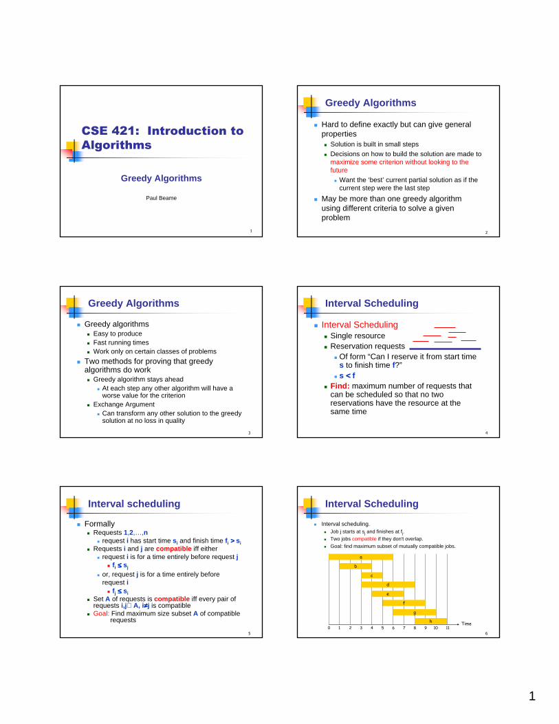
� Interval scheduling.� Job j starts at sj and finishes at fj.� Two jobs compatible if they don't overlap.� Goal: find maximum subset of mutually compatible jobs.

Time0 1 2 3 4 5 6 7 8 9 10 11

f

g

h

e

a

b

c

d

2

7

Greedy Algorithms for Interval Scheduling

� What criterion should we try?� Earliest start time s i

� Shortest request time f i-s i

� Earliest finish fime f i

8

Greedy Algorithms for Interval Scheduling

� What criterion should we try?� Earliest start time s i

� Doesn’t work

� Shortest request time f i-s i� Doesn’t work

� Even fewest conflicts doesn’t work

� Earliest finish fime f i� Works

9

Greedy Algorithm for Interval Scheduling

R←set of all requestsA←∅While R≠∅ do

Choose request i∈∈∈∈R with smallest finishing time f i

Add request i to ADelete all requests in R that are not

compatible with request iReturn A

10

Greedy Algorithm for Interval Scheduling

� Claim: A is a compatible set of requests and these are added to A in order of finish time� When we add a request to A we delete all

incompatible ones from R

� Claim: For any other set O⊆⊆⊆⊆R of compatible requests then if we order requests in A and Oby finish time then for each k:� If O contains a k th request then so does A and

� the finish time of the k th request in A, is ≤≤≤≤ the finish time of the k th request in O, i.e. “ak ≤≤≤≤ ok”where ak and ok are the respective finish times

Enough to prove that A is optimal

11

Inductive Proof of Claim: a k≤≤≤≤ok

� Base Case: This is true for the first request in A since that is the one with the smallest finish time

� Inductive Step: Suppose ak≤≤≤≤ok� By definition of compatibility

� If O contains a k+1st request r then the start time of that request must be after ok and thus after ak

� Thus r is compatible with the first k requests in A� Therefore

� A has at least k+1 requests since a compatible one is available after the first k are chosen

� r was among those considered by the greedy algorithm for that k+1st request in A

� Therefore by the greedy choice the finish time of r which is ok+1 is at least the finish time of that k+1st request in Awhich is ak+1

12

Interval Scheduling: Analysis

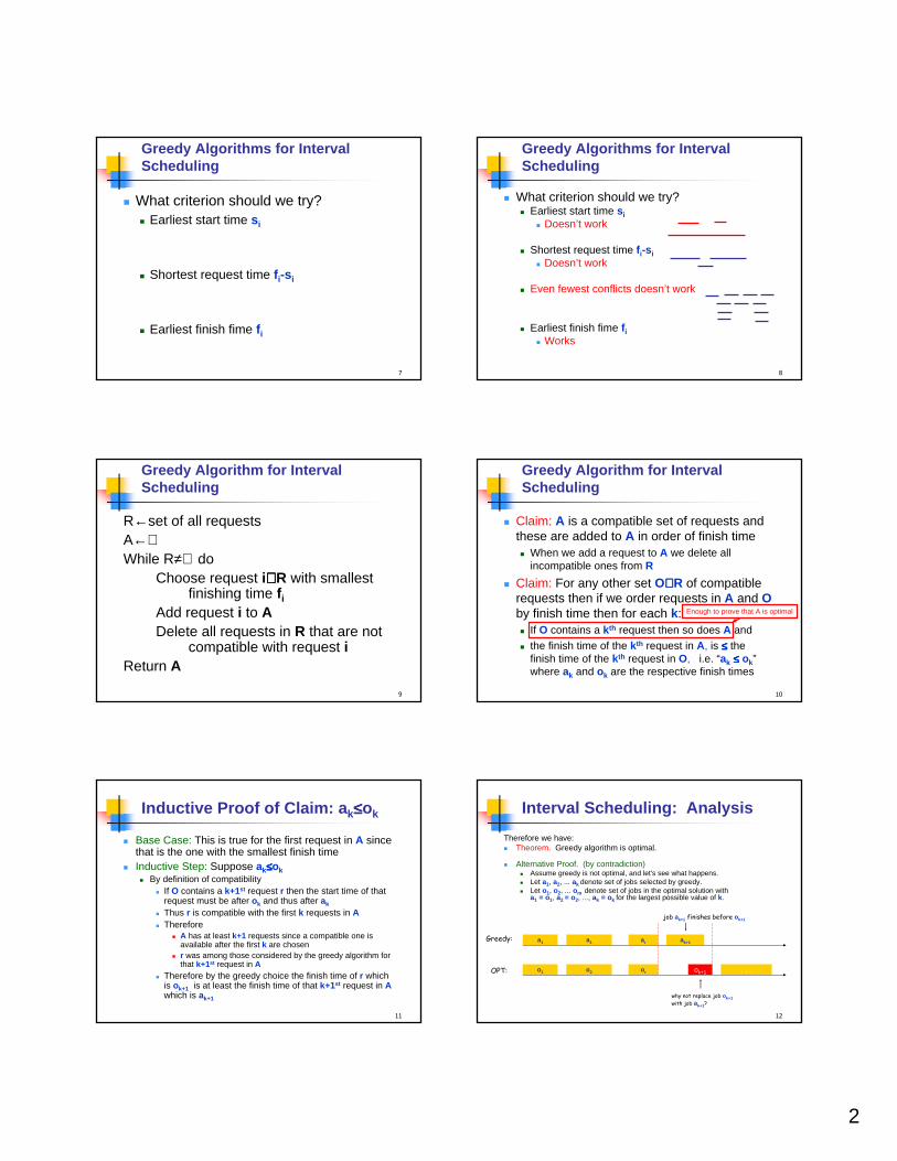
Therefore we have:� Theorem. Greedy algorithm is optimal.

� Alternative Proof. (by contradiction)� Assume greedy is not optimal, and let's see what happens.� Let a1, a2, ... ak denote set of jobs selected by greedy.� Let o1, o2, ... om denote set of jobs in the optimal solution with

a1 = o1, a2 = o2, ..., ak = ok for the largest possible value of k.

o1 o2 or

a1 a1 ar ak+1

. . .

Greedy:

OPT: ok+1

why not replace job ok+1with job ak+1?

job ak+1 finishes before ok+1

3

13

Implementing the Greedy Algorithm

� Sort the requests by finish time� O(nlog n ) time

� Maintain current latest finish time scheduled� Keep array of start times indexed by request

number� Only eliminate incompatible requests as

needed� Walk along array of requests sorted by finish times

skipping those whose start time is before current latest finish time scheduled

� O(n) additional time for greedy algorithm

14

Sort jobs by finish times so that 0 ≤≤≤≤ f1 ≤≤≤≤ f2 ≤≤≤≤ ... ≤≤≤≤ fn.

A ←←←← φφφφlast ←←←← 0for j = 1 to n {

if (last ≤≤≤≤ sj)A ←←←← A ∪∪∪∪ {j}last ←←←← fj

}return A

Interval Scheduling: Greedy Algorithm Implementation

O(n log n)

O(n)

15

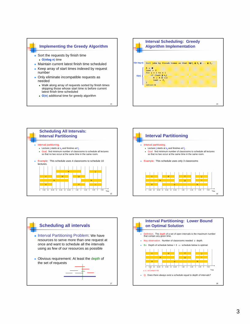
Scheduling All Intervals:Interval Partitioning

� Interval partitioning.� Lecture j starts at s j and finishes at f j.� Goal: find minimum number of classrooms to schedule all lectures

so that no two occur at the same time in the same room.

� Example: This schedule uses 4 classrooms to schedule 10 lectures.

Time9 9:30 10 10:30 11 11:30 12 12:30 1 1:30 2 2:30

h

c

b

a

e

d g

f i

j

3 3:30 4 4:30

16

Interval Partitioning

� Interval partitioning.� Lecture j starts at s j and finishes at f j.� Goal: find minimum number of classrooms to schedule all lectures

so that no two occur at the same time in the same room.

� Example: This schedule uses only 3 classrooms

Time9 9:30 10 10:30 11 11:30 12 12:30 1 1:30 2 2:30

h

c

a e

f

g i

j

3 3:30 4 4:30

d

b

17

Scheduling all intervals

� Interval Partitioning Problem: We have resources to serve more than one request at once and want to schedule all the intervals using as few of our resources as possible

� Obvious requirement: At least the depth of the set of requests

18

Interval Partitioning: Lower Bound on Optimal Solution

� Definition. The depth of a set of open intervals is the maximum number that contain any given time.

� Key observation. Number of classrooms needed ≥ depth.

� Ex: Depth of schedule below = 3 ⇒ schedule below is optimal.

� Q. Does there always exist a schedule equal to depth of intervals?

Time

9 9:30 10 10:30 11 11:30 12 12:30 1 1:30 2 2:30

h

c

a e

f

g i

j

3 3:30 4 4:30

d

b

a, b, c all contain 9:30

4

19

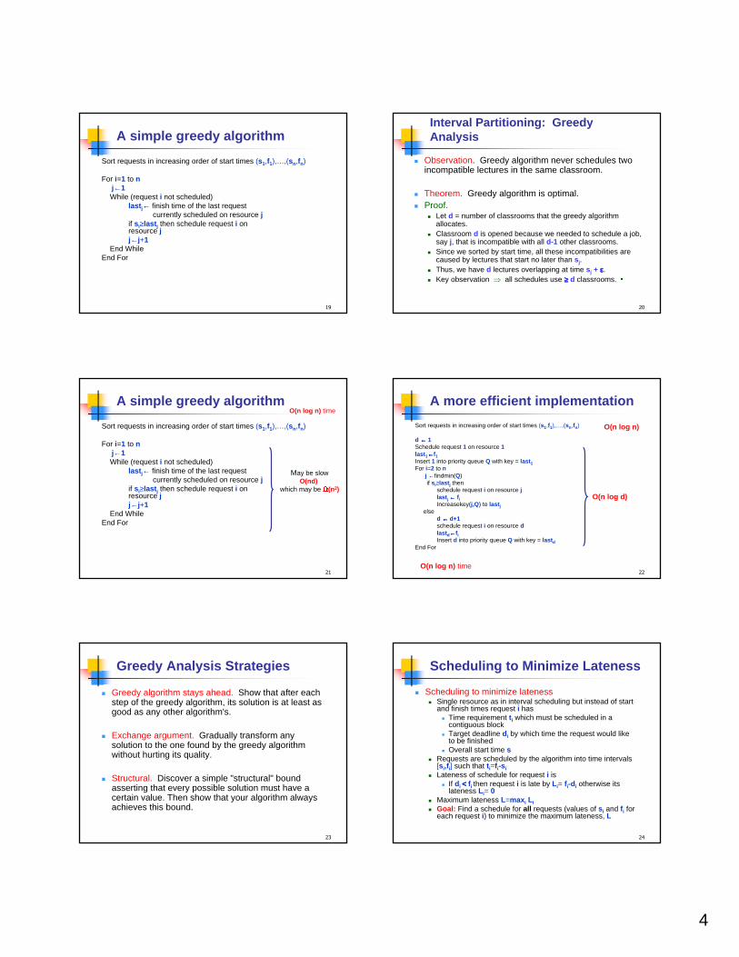
A simple greedy algorithm

Sort requests in increasing order of start times (s1,f1),…,(sn,fn)

For i=1 to nj←1While (request i not scheduled)

last j← finish time of the last request currently scheduled on resource j

if s i≥last j then schedule request i on resource jj←j+1

End WhileEnd For

20

Interval Partitioning: Greedy Analysis

� Observation. Greedy algorithm never schedules two incompatible lectures in the same classroom.

� Theorem. Greedy algorithm is optimal.� Proof.

� Let d = number of classrooms that the greedy algorithm allocates.

� Classroom d is opened because we needed to schedule a job, say j, that is incompatible with all d-1 other classrooms.

� Since we sorted by start time, all these incompatibilities are caused by lectures that start no later than s j.

� Thus, we have d lectures overlapping at time s j + εεεε.� Key observation ⇒ all schedules use ≥≥≥≥ d classrooms. ▪

21

A simple greedy algorithm


For i=1 to nj←1While (request i not scheduled)

last j← finish time of the last request currently scheduled on resource j

if s i≥last j then schedule request i on resource jj←j+1

End WhileEnd For

O(n log n) time

May be slowO(nd)

which may be �

(n2)

22

A more efficient implementation


d ←←←← 1Schedule request 1 on resource 1last 1←←←←f1Insert 1 into priority queue Q with key = last 1For i=2 to n

j ←findmin(Q)if s i≥last j then

schedule request i on resource jlast j ←←←← f iIncreasekey(j,Q) to last j

elsed ←←←← d+1schedule request i on resource dlast d←←←←f iInsert d into priority queue Q with key = last d

End For

O(n log n) time

O(n log d)

O(n log n)

23

Greedy Analysis Strategies

� Greedy algorithm stays ahead. Show that after each step of the greedy algorithm, its solution is at least as good as any other algorithm's.

� Exchange argument. Gradually transform any solution to the one found by the greedy algorithm without hurting its quality.

� Structural. Discover a simple "structural" bound asserting that every possible solution must have a certain value. Then show that your algorithm always achieves this bound.

24

Scheduling to Minimize Lateness

� Scheduling to minimize lateness� Single resource as in interval scheduling but instead of start

and finish times request i has� Time requirement t i which must be scheduled in a

contiguous block� Target deadline d i by which time the request would like

to be finished� Overall start time s

� Requests are scheduled by the algorithm into time intervals [s i,f i] such that t i=f i-s i

� Lateness of schedule for request i is� If d i <<<< f i then request i is late by L i= f i-d i otherwise its

lateness L i= 0� Maximum lateness L=max i L i� Goal: Find a schedule for all requests (values of s i and f i for

each request i) to minimize the maximum lateness, L

5

25

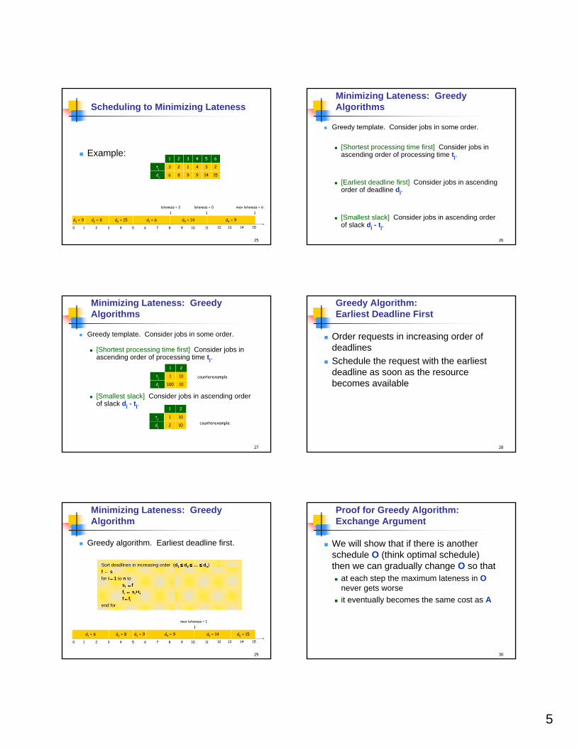
Scheduling to Minimizing Lateness

� Example:

0 1 2 3 4 5 6 7 8 9 10 11 12 13 14 15

d5 = 14d2 = 8 d6 = 15 d1 = 6 d4 = 9d3 = 9

lateness = 0lateness = 2

dj 6

tj 3

1

8

2

2

9

1

3

9

4

4

14

3

5

15

2

6

max lateness = 6

26

Minimizing Lateness: Greedy Algorithms

� Greedy template. Consider jobs in some order.

� [Shortest processing time first] Consider jobs in ascending order of processing time t j.

� [Earliest deadline first] Consider jobs in ascending order of deadline d j.

� [Smallest slack] Consider jobs in ascending order of slack d j - t j.

27

� Greedy template. Consider jobs in some order.

� [Shortest processing time first] Consider jobs in ascending order of processing time t j.

� [Smallest slack] Consider jobs in ascending order of slack d j - t j.

Minimizing Lateness: Greedy Algorithms

counterexample

dj

tj

100

1

1

10

10

2

counterexampledj

tj

2

1

1

10

10

2

28

Greedy Algorithm: Earliest Deadline First

� Order requests in increasing order of deadlines

� Schedule the request with the earliest deadline as soon as the resource becomes available

29

0 1 2 3 4 5 6 7 8 9 10 11 12 13 14 15

d5 = 14d2 = 8 d6 = 15d1 = 6 d4 = 9d3 = 9

max lateness = 1

Sort deadlines in increasing order (d1 ≤≤≤≤ d2 ≤≤≤≤ … ≤≤≤≤ dn)

f ← sfor i←←←←1 to n to

s i ←←←←ff i ←←←← s i+t i

f←←←←f i

end for

Minimizing Lateness: Greedy Algorithm

� Greedy algorithm. Earliest deadline first.

30

Proof for Greedy Algorithm: Exchange Argument

� We will show that if there is another schedule O (think optimal schedule) then we can gradually change O so that � at each step the maximum lateness in O

never gets worse� it eventually becomes the same cost as A

6

31

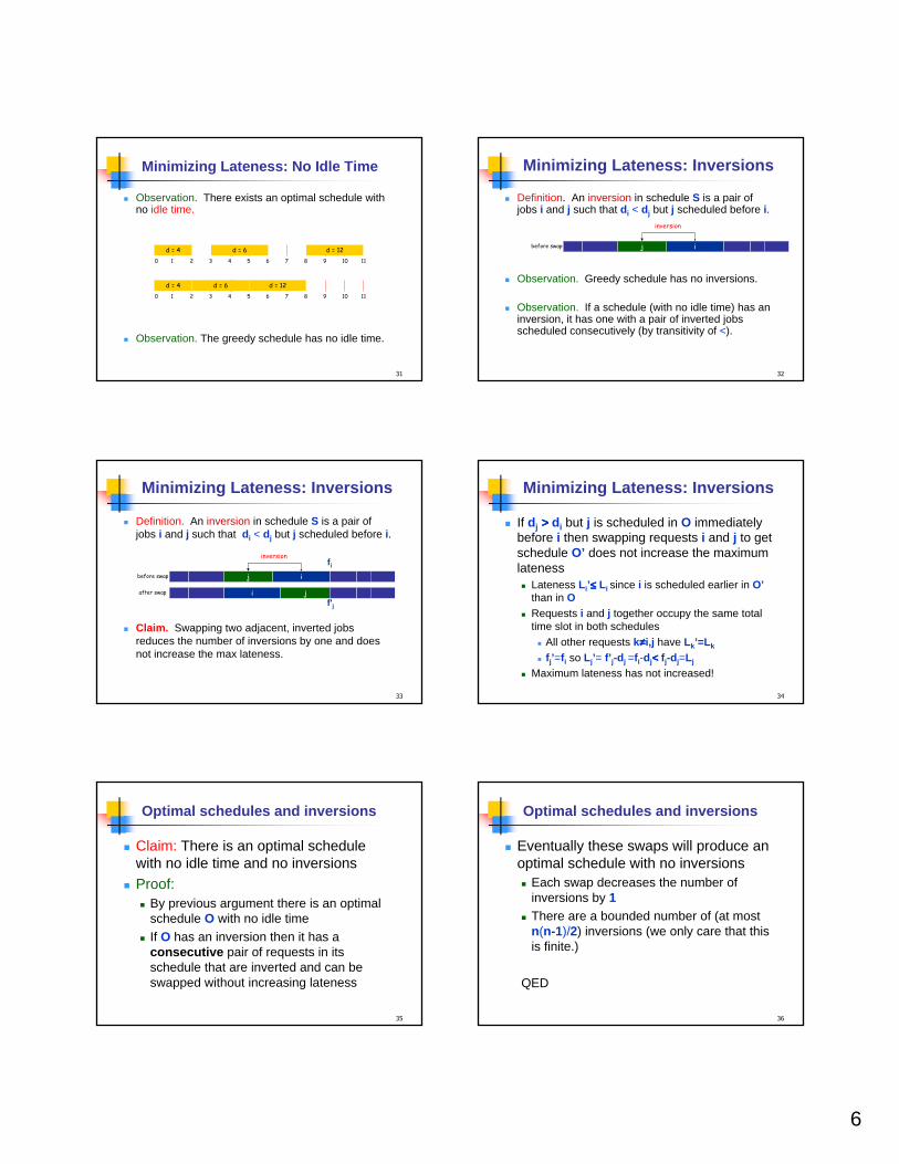
Minimizing Lateness: No Idle Time

� Observation. There exists an optimal schedule with no idle time.

� Observation. The greedy schedule has no idle time.

0 1 2 3 4 5 6

d = 4 d = 6

7 8 9 10 11

d = 12

0 1 2 3 4 5 6

d = 4 d = 6

7 8 9 10 11

d = 12

32

Minimizing Lateness: Inversions

� Definition. An inversion in schedule S is a pair of jobs i and j such that d i < d j but j scheduled before i.

� Observation. Greedy schedule has no inversions.

� Observation. If a schedule (with no idle time) has an inversion, it has one with a pair of inverted jobs scheduled consecutively (by transitivity of <).

ijbefore swap

inversion

33


� Definition. An inversion in schedule S is a pair of jobs i and j such that d i < d j but j scheduled before i.

� Claim. Swapping two adjacent, inverted jobs reduces the number of inversions by one and does not increase the max lateness.

ij

i j

before swap

after swap

f' j

f i

inversion

34


� If d j >>>> d i but j is scheduled in O immediately before i then swapping requests i and j to get schedule O’ does not increase the maximum lateness� Lateness L i’≤≤≤≤ L i since i is scheduled earlier in O’

than in O� Requests i and j together occupy the same total

time slot in both schedules

� All other requests k≠≠≠≠i,j have Lk’=L k

� f j’=f i so L j’= f’ j-d j =f i-d j<<<< f j-d j=L j

� Maximum lateness has not increased!

35

Optimal schedules and inversions

� Claim: There is an optimal schedule with no idle time and no inversions

� Proof:� By previous argument there is an optimal

schedule O with no idle time� If O has an inversion then it has a

consecutive pair of requests in its schedule that are inverted and can be swapped without increasing lateness

36

Optimal schedules and inversions

� Eventually these swaps will produce an optimal schedule with no inversions� Each swap decreases the number of

inversions by 1� There are a bounded number of (at most

n(n-1)/2) inversions (we only care that this is finite.)

QED

7

37

Idleness and Inversions are the only issue

� Claim: All schedules with no inversions and no idle time have the same maximum lateness

� Proof� Schedules can differ only in how they order requests with

equal deadlines� Consider all requests having some common deadline d

� Maximum lateness of these jobs is based only on the finish time of the last of these jobs but the set of these requests occupies the same time segment in both schedules

� Last of these requests finishes at the same time in any such schedule.

38

Earliest Deadline First is optimal

� We know that� There is an optimal schedule with no idle

time or inversions� All schedules with no idle time or

inversions have the same maximum lateness

� EDF produces a schedule with no idle time or inversions

� Therefore � EDF produces an optimal schedule

39

Optimal Caching/Paging

� Memory systems � many levels of storage with different access times� smaller storage has shorter access time� to access an item it must be brought to the lowest

level of the memory system� Consider the management problem between

adjacent levels� Main memory with n data items from a set U� Cache can hold k<<<<n items� Simplest version with no direct-mapping or other

restrictions about where items can be� Suppose cache is full initially

� Holds k data items to start with

40

Optimal Caching/Paging

� Given a memory request d from U� If d is stored in the cache we can access it quickly� If not then we call it a cache miss and (since the

cache is full) � we must bring it into cache and evict some

other data item from the cache� which one to evict?

� Given a sequence D=d1,d2,…,dm of elements from U corresponding to memory requests

� Find a sequence of evictions (an eviction schedule) that has as few cache misses as possible

41

Caching Example

� n=3, k=2, U={a,b,c}� Cache initially contains {a,b}� D= a b c b c a b� S= a c� C= a b a

b c b

� This is optimal

42

A Note on Optimal Caching

� In real operating conditions one typically needs an on-line algorithm� make the eviction decisions as each memory

request arrives

� However to design and analyze these algorithms it is also important to understand how the best possible decisions can be made if one did know the future� Field of on-line algorithms compares the quality of

on-line decisions to that of the optimal schedule

� What does an optimal schedule look like?

8

43

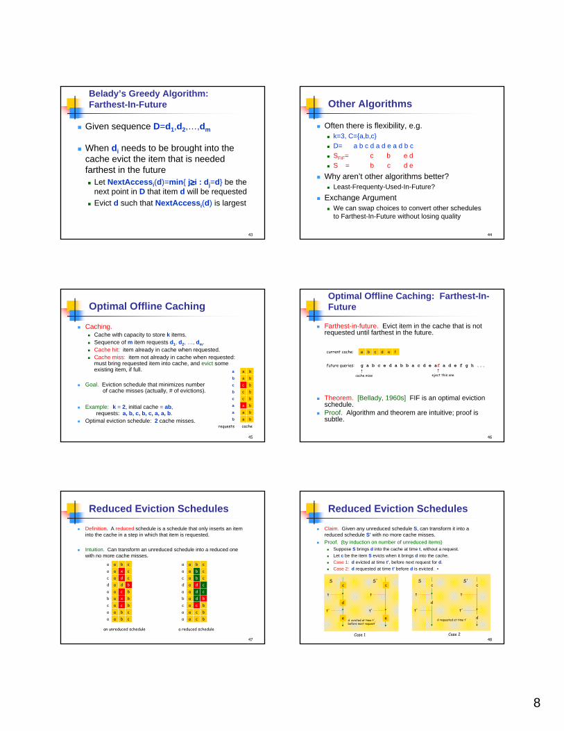
Belady’s Greedy Algorithm:Farthest-In-Future

� Given sequence D=d1,d2,…,dm

� When d i needs to be brought into the cache evict the item that is needed farthest in the future� Let NextAccess i(d)=min { j≥≥≥≥i : d j=d} be the

next point in D that item d will be requested� Evict d such that NextAccess i(d) is largest

44

Other Algorithms

� Often there is flexibility, e.g.� k=3, C={a,b,c} � D= a b c d a d e a d b c� SFIF= c b e d� S = b c d e

� Why aren’t other algorithms better?� Least-Frequenty-Used-In-Future?

� Exchange Argument� We can swap choices to convert other schedules

to Farthest-In-Future without losing quality

45

Optimal Offline Caching

� Caching.� Cache with capacity to store k items.� Sequence of m item requests d1, d2, …, dm.� Cache hit: item already in cache when requested.� Cache miss: item not already in cache when requested:

must bring requested item into cache, and evict some existing item, if full.

� Goal. Eviction schedule that minimizes number of cache misses (actually, # of evictions).

� Example: k = 2, initial cache = ab,requests: a, b, c, b, c, a, a, b .

� Optimal eviction schedule: 2 cache misses.

a b

a b

c b

c b

c b

a b

a

b

c

b

c

a

a ba

a bb

cacherequests

46

Optimal Offline Caching: Farthest-In-Future

� Farthest-in-future. Evict item in the cache that is not requested until farthest in the future.

� Theorem. [Bellady, 1960s] FIF is an optimal eviction schedule.

� Proof. Algorithm and theorem are intuitive; proof is subtle.

a b

g a b c e d a b b a c d e a f a d e f g h ...

current cache: c d e f

future queries:

cache miss eject this one

47

Reduced Eviction Schedules

� Definition. A reduced schedule is a schedule that only inserts an item into the cache in a step in which that item is requested.

� Intuition. Can transform an unreduced schedule into a reduced one with no more cache misses.

a x

an unreduced schedule

c

a d c

a d b

a c b

a x b

a c b

a b c

a b c

a

c

d

a

b

c

a

a

a b

a reduced schedule

c

a b c

a d c

a d c

a d b

a c b

a c b

a c b

a

c

d

a

b

c

a

a

a b ca a b ca

48

Reduced Eviction Schedules

� Claim. Given any unreduced schedule S, can transform it into a reduced schedule S' with no more cache misses.

� Proof. (by induction on number of unreduced items)� Suppose S brings d into the cache at time t, without a request.

� Let c be the item S evicts when it brings d into the cache.

� Case 1: d evicted at time t' , before next request for d.

� Case 2: d requested at time t' before d is evicted. ▪t

t'

d

c

t

t'

cS'

d

S

d requested at time t'

t

t'

d

c

t

t'

cS'

e

S

d evicted at time t',before next request

e

Case 1 Case 2

9

49

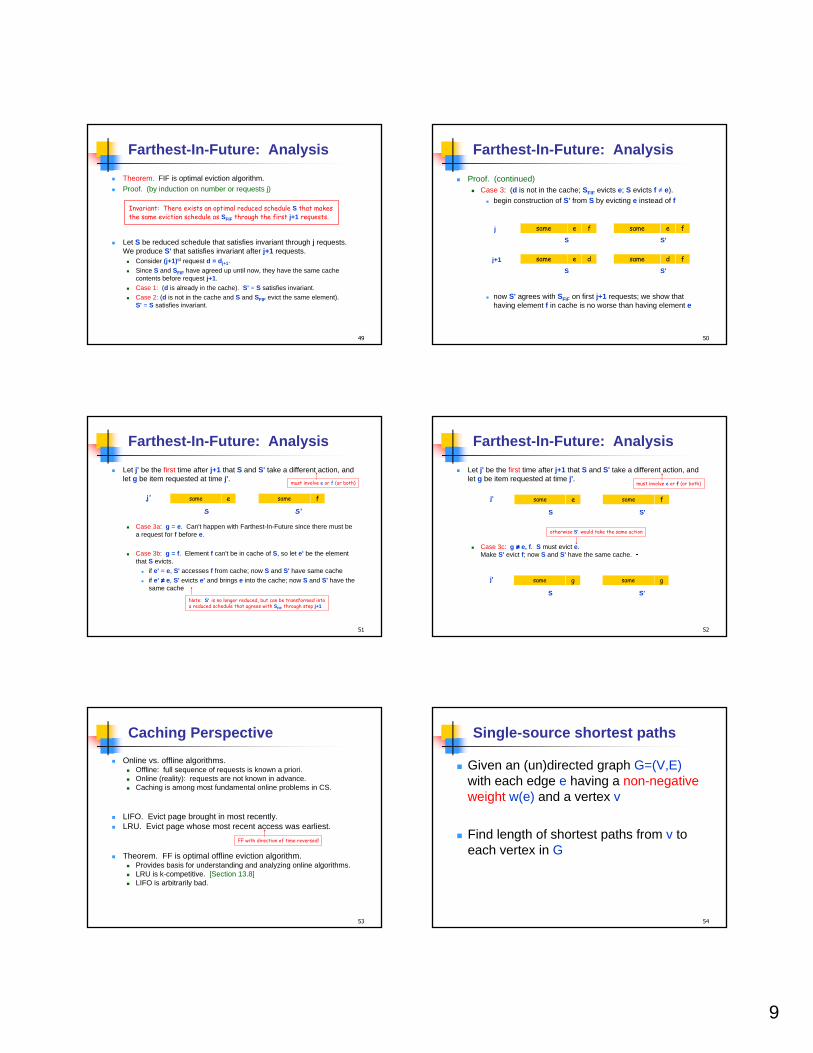
Farthest-In-Future: Analysis

� Theorem. FIF is optimal eviction algorithm.

� Proof. (by induction on number or requests j)

� Let S be reduced schedule that satisfies invariant through j requests. We produce S' that satisfies invariant after j+1 requests.

� Consider (j+1)st request d = d j+1.

� Since S and SFIF have agreed up until now, they have the same cache contents before request j+1.

� Case 1: (d is already in the cache). S' = S satisfies invariant.

� Case 2: (d is not in the cache and S and SFIF evict the same element).S' = S satisfies invariant.

Invariant: There exists an optimal reduced schedule S that makes the same eviction schedule as SFIF through the first j+1 requests.

50


� Proof. (continued)� Case 3: (d is not in the cache; SFIF evicts e; S evicts f ≠ e).

� begin construction of S' from S by evicting e instead of f

� now S' agrees with SFIF on first j+1 requests; we show that having element f in cache is no worse than having element e

j same f same fee

S S'

j same d same fde

S S'

j+1

51


� Let j' be the first time after j+1 that S and S' take a different action, and let g be item requested at time j' .

� Case 3a: g = e. Can't happen with Farthest-In-Future since there must be a request for f before e.

� Case 3b: g = f . Element f can't be in cache of S, so let e' be the element that S evicts.

� if e' = e, S' accesses f from cache; now S and S' have same cache

� if e' ≠≠≠≠ e, S' evicts e' and brings e into the cache; now S and S' have the same cache

Note: S' is no longer reduced, but can be transformed intoa reduced schedule that agrees with SFIF through step j+1

same e same f

S S'

j'

must involve e or f (or both)

52


� Let j' be the first time after j+1 that S and S' take a different action, and let g be item requested at time j' .

� Case 3c: g ≠≠≠≠ e, f. S must evict e.Make S' evict f; now S and S' have the same cache. ▪

same g same g

S S'

j'

otherwise S' would take the same action

same e same f

S S'

j'

must involve e or f (or both)

53

Caching Perspective

� Online vs. offline algorithms.� Offline: full sequence of requests is known a priori.� Online (reality): requests are not known in advance.� Caching is among most fundamental online problems in CS.

� LIFO. Evict page brought in most recently.� LRU. Evict page whose most recent access was earliest.

� Theorem. FF is optimal offline eviction algorithm.� Provides basis for understanding and analyzing online algorithms.� LRU is k-competitive. [Section 13.8]� LIFO is arbitrarily bad.

FF with direction of time reversed!

54

Single-source shortest paths

� Given an (un)directed graph G=(V,E)with each edge e having a non-negativeweight w(e) and a vertex v

� Find length of shortest paths from v to each vertex in G

10

55

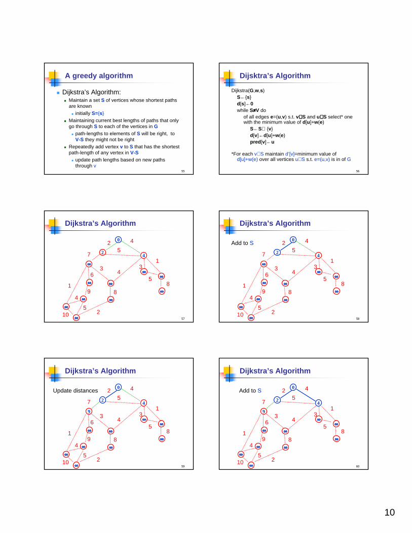
A greedy algorithm

� Dijkstra’s Algorithm:� Maintain a set S of vertices whose shortest paths

are known� initially S={s}

� Maintaining current best lengths of paths that only go through S to each of the vertices in G

� path-lengths to elements of S will be right, to V-S they might not be right

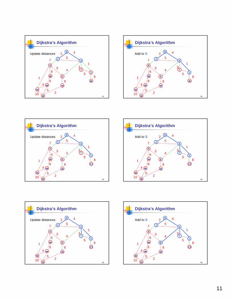
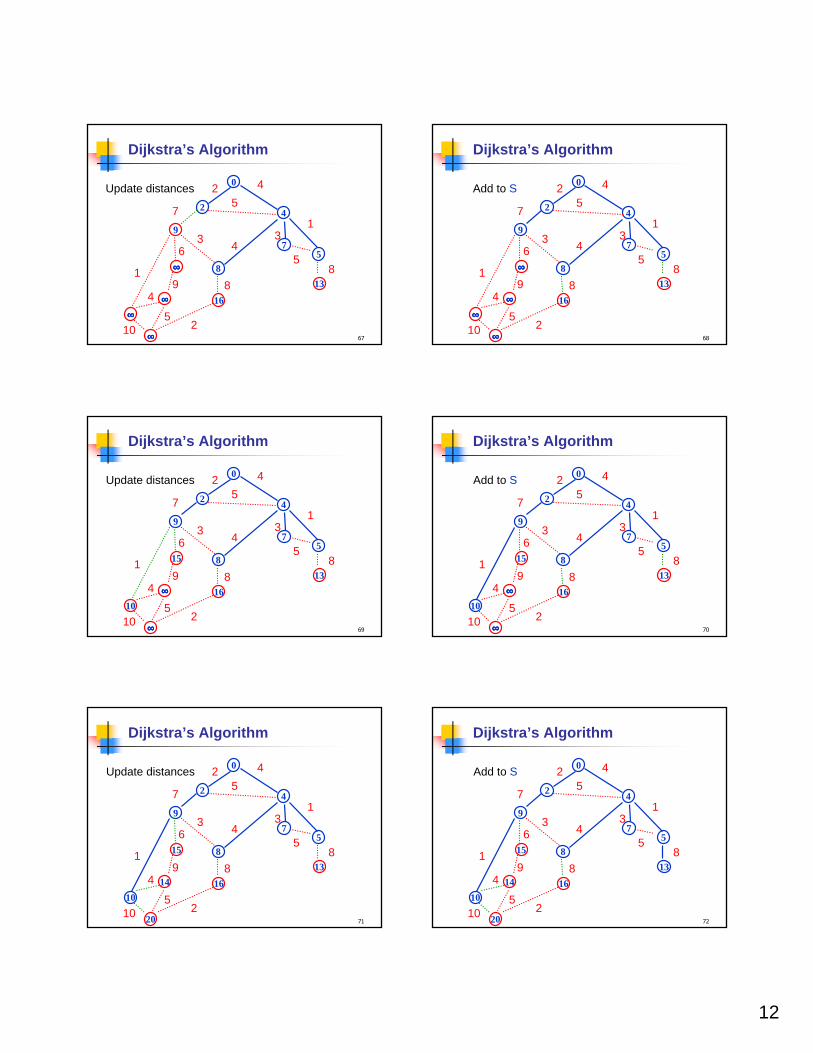
� Repeatedly add vertex v to S that has the shortest path-length of any vertex in V-S

� update path lengths based on new paths through v

56

Dijsktra’s Algorithm

Dijkstra(G,w,s)S←{s}d[s]←0while S≠≠≠≠V do

of all edges e=(u,v) s.t. v∉∉∉∉S and u∈∈∈∈S select* one with the minimum value of d[u]+w(e)

S←S∪ {v}d[v]←d[u]+w(e)pred [v]←u

*For each v∉S maintain d’[v]=minimum value of d[u]+w(e) over all vertices u∈S s.t. e=(u,v) is in of G

57

Dijkstra’s Algorithm

2

7

1

43

4

5

13

58

6

94

5210

8

0

24

∞∞∞∞

∞∞∞∞

∞∞∞∞

∞∞∞∞

∞∞∞∞∞∞∞∞

∞∞∞∞

∞∞∞∞∞∞∞∞

∞∞∞∞

58


2

7

1

43

4

5

13

58

6

94

5210

8

0

24

∞∞∞∞

∞∞∞∞

∞∞∞∞

∞∞∞∞

∞∞∞∞∞∞∞∞

∞∞∞∞

∞∞∞∞∞∞∞∞

∞∞∞∞

Add to S

59


2

7

1

43

4

5

13

58

6

94

5210

8

0

24

∞∞∞∞

∞∞∞∞

9

∞∞∞∞

∞∞∞∞∞∞∞∞

∞∞∞∞

∞∞∞∞∞∞∞∞

∞∞∞∞

Update distances

60


2

7

1

43

4

5

13

58

6

94

5210

8

0

24

∞∞∞∞

∞∞∞∞

9

∞∞∞∞

∞∞∞∞∞∞∞∞

∞∞∞∞

∞∞∞∞∞∞∞∞

∞∞∞∞

Add to S

11

61


2

7

1

43

4

5

13

58

6

94

5210

8

0

24

∞∞∞∞

8

9

∞∞∞∞

∞∞∞∞∞∞∞∞

∞∞∞∞

75

∞∞∞∞

Update distances

62


2

7

1

43

4

5

13

58

6

94

5210

8

0

24

∞∞∞∞

8

9

∞∞∞∞

∞∞∞∞∞∞∞∞

∞∞∞∞

75

∞∞∞∞

Add to S

63


2

7

1

43

4

5

13

58

6

94

5210

8

0

24

∞∞∞∞

8

9

∞∞∞∞

∞∞∞∞∞∞∞∞

∞∞∞∞

75

13

Update distances

64


2

7

1

43

4

5

13

58

6

94

5210

8

0

24

∞∞∞∞

8

9

∞∞∞∞

∞∞∞∞∞∞∞∞

∞∞∞∞

75

13

Add to S

65


2

7

1

43

4

5

13

58

6

94

5210

8

0

24

∞∞∞∞

8

9

∞∞∞∞

∞∞∞∞∞∞∞∞

∞∞∞∞

75

13

Update distances

66


2

7

1

43

4

5

13

58

6

94

5210

8

0

24

∞∞∞∞

8

9

∞∞∞∞

∞∞∞∞∞∞∞∞

∞∞∞∞

75

13

Add to S

12

67


2

7

1

43

4

5

13

58

6

94

5210

8

0

24

16

8

9

∞∞∞∞

∞∞∞∞∞∞∞∞

∞∞∞∞

75

13

Update distances

68


2

7

1

43

4

5

13

58

6

94

5210

8

0

24

16

8

9

∞∞∞∞

∞∞∞∞∞∞∞∞

∞∞∞∞

75

13

Add to S

69


2

7

1

43

4

5

13

58

6

94

5210

8

0

24

16

8

9

15

∞∞∞∞10

∞∞∞∞

75

13

Update distances

70


2

7

1

43

4

5

13

58

6

94

5210

8

0

24

16

8

9

15

∞∞∞∞10

∞∞∞∞

75

13

Add to S

71


2

7

1

43

4

5

13

58

6

94

5210

8

0

24

16

8

9

15

14

10

20

75

13

Update distances

72


2

7

1

43

4

5

13

58

6

94

5210

8

0

24

16

8

9

15

14

10

20

75

13

Add to S

13

73


2

7

1

43

4

5

13

58

6

94

5210

8

0

24

16

8

9

15

14

10

20

75

13

Update distances

74


2

7

1

43

4

5

13

58

6

94

5210

8

0

24

16

8

9

15

14

10

20

75

13

Add to S

75


2

7

1

43

4

5

13

58

6

94

5210

8

0

24

16

8

9

15

14

10

19

75

13

Update distances

76


2

7

1

43

4

5

13

58

6

94

5210

8

0

24

16

8

9

15

14

10

19

75

13

Add to S

77


2

7

1

43

4

5

13

58

6

94

5210

8

0

24

16

8

9

15

14

10

19

75

13

Update distances

78


2

7

1

43

4

5

13

58

6

94

5210

8

0

24

16

8

9

15

14

10

19

75

13

Add to S

14

79


2

7

1

43

4

5

13

58

6

94

5210

8

0

24

16

8

9

15

14

10

18

75

13

Update distances

80


2

7

1

43

4

5

13

58

6

94

5210

8

0

24

16

8

9

15

14

10

18

75

13

Add to S

81

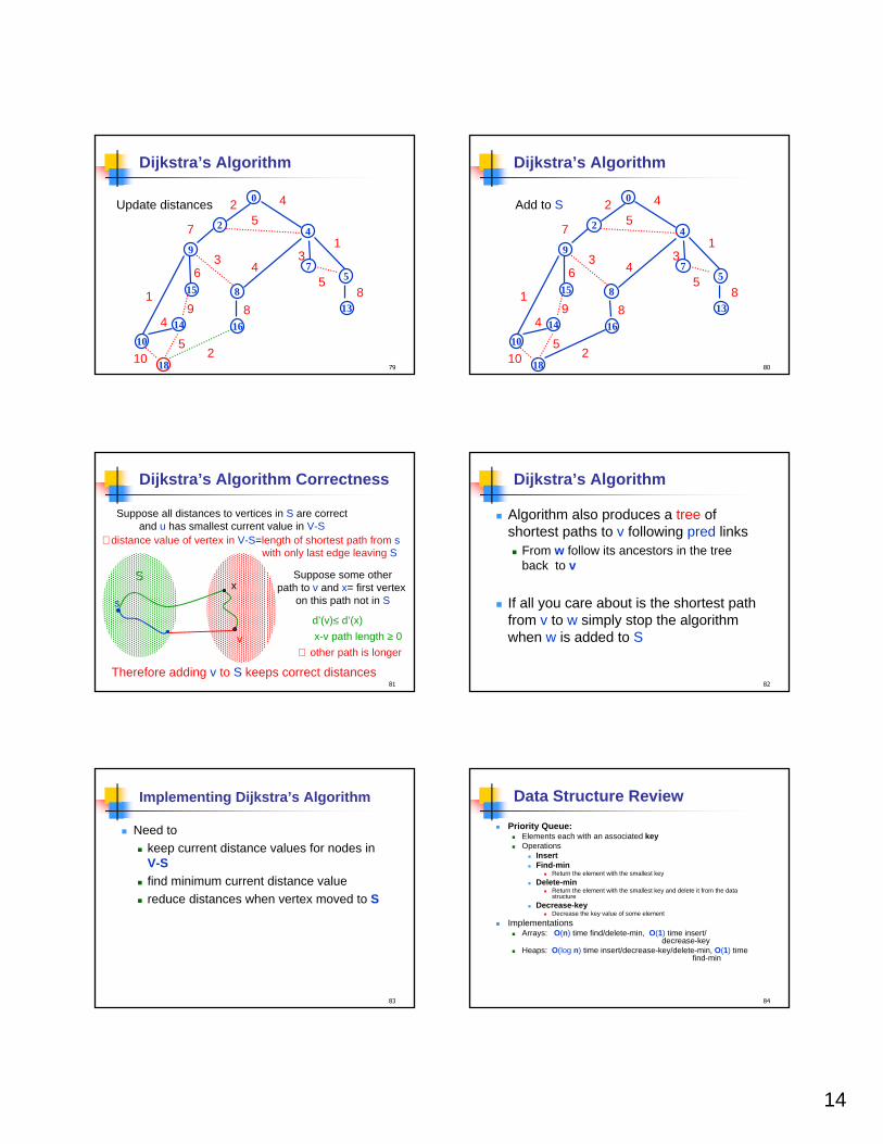
Dijkstra’s Algorithm Correctness

Suppose all distances to vertices in S are correctand u has smallest current value in V-S

d’(v)≤ d’(x)

x-v path length ≥ 0

∴distance value of vertex in V-S=length of shortest path from swith only last edge leaving S

s

v

xS Suppose some other

path to v and x= first vertex on this path not in S

∴ other path is longer

Therefore adding v to S keeps correct distances82


� Algorithm also produces a tree of shortest paths to v following pred links� From w follow its ancestors in the tree

back to v

� If all you care about is the shortest path from v to w simply stop the algorithm when w is added to S

83

Implementing Dijkstra’s Algorithm

� Need to � keep current distance values for nodes in

V-S� find minimum current distance value� reduce distances when vertex moved to S

84

Data Structure Review

� Priority Queue:� Elements each with an associated key� Operations

� Insert� Find-min

� Return the element with the smallest key

� Delete-min� Return the element with the smallest key and delete it from the data

structure

� Decrease-key� Decrease the key value of some element

� Implementations� Arrays: O(n) time find/delete-min, O(1) time insert/

decrease-key� Heaps: O(log n) time insert/decrease-key/delete-min, O(1) time

find-min

15

85

Dijkstra’s Algorithm with Priority Queues

� For each vertex u not in tree maintain cost of current cheapest path through tree to u� Store u in priority queue with key = length

of this path� Operations:

� n-1 insertions (each vertex added once)� n-1 delete-mins (each vertex deleted once)

� pick the vertex of smallest key, remove it from the priority queue and add its edge to the graph

� <m decrease-keys (each edge updates one vertex)

86

Dijskstra’s Algorithm with Priority Queues

� Priority queue implementations� Array

� insert O(1), delete-min O(n), decrease-key O(1)� total O(n+n2+m)=O(n2)

� Heap� insert, delete-min, decrease-key all O(log n)� total O(m log n)

� d-Heap (d=m/n)� insert, decrease-key O(logm/n n)� delete-min O((m/n) logm/n n)� total O(m logm/n n)

87

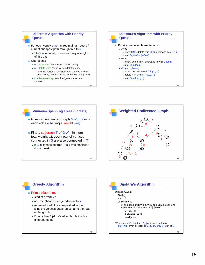
Minimum Spanning Trees (Forests)

� Given an undirected graph G=(V,E) with each edge e having a weight w(e)

� Find a subgraph T of G of minimum total weight s.t. every pair of vertices connected in G are also connected in T� if G is connected then T is a tree otherwise

it is a forest

88

Weighted Undirected Graph

2

7

-1

43

4

5

13

58

6

94

579

8

1

23

10

5

4

9

12

8

13

67

11

89

Greedy Algorithm

� Prim’s Algorithm:� start at a vertex s� add the cheapest edge adjacent to s� repeatedly add the cheapest edge that

joins the vertices explored so far to the rest of the graph

� Exactly like Dijsktra’s Algorithm but with a different metric

90

Dijsktra’s Algorithm

Dijkstra(G,w,s)S←{s}d[s]←0while S≠≠≠≠V do

of all edges e=(u,v) s.t. v∉∉∉∉S and u∈∈∈∈S select* one with the minimum value of d[u]+w(e)

S←S∪ {v}d[v]←d[u]+w(e)pred [v]←u

*For each v∉S maintain d’[v]=minimum value of d[u]+w(e) over all vertices u∈S s.t. e=(u,v) is in of G

16

91

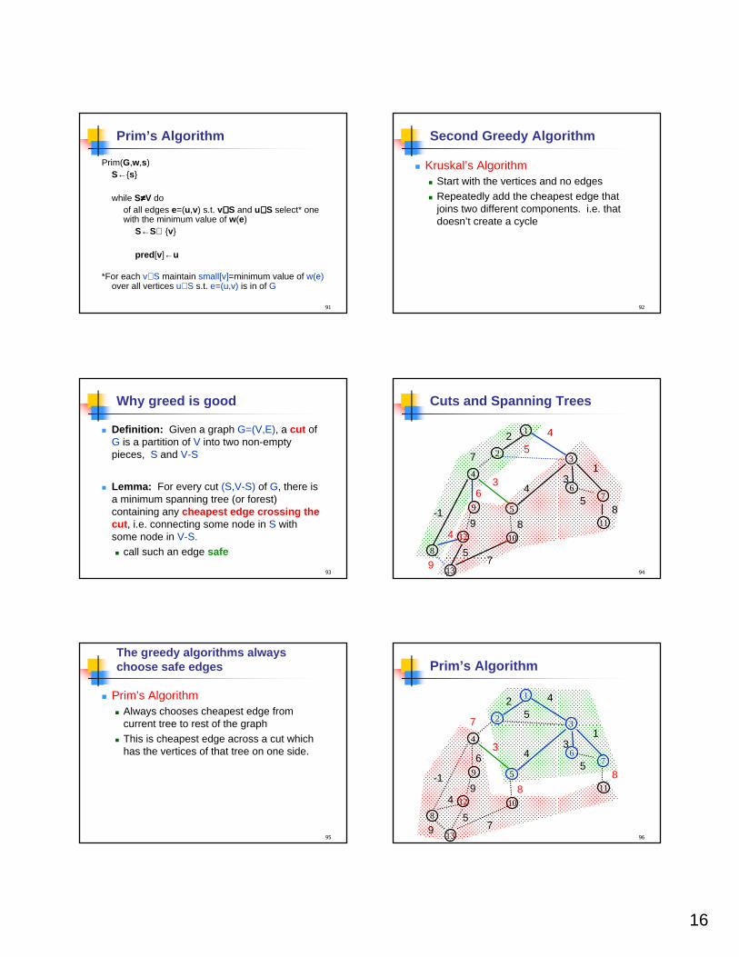
Prim’s Algorithm

Prim(G,w,s)S←{s}

while S≠≠≠≠V doof all edges e=(u,v) s.t. v∉∉∉∉S and u∈∈∈∈S select* one with the minimum value of w(e)

S←S∪ {v}

pred [v]←u

*For each v∉S maintain small[v]=minimum value of w(e)over all vertices u∈S s.t. e=(u,v) is in of G

92

Second Greedy Algorithm

� Kruskal’s Algorithm� Start with the vertices and no edges� Repeatedly add the cheapest edge that

joins two different components. i.e. that doesn’t create a cycle

93

Why greed is good

� Definition: Given a graph G=(V,E), a cut of G is a partition of V into two non-empty pieces, S and V-S

� Lemma: For every cut (S,V-S) of G, there is a minimum spanning tree (or forest) containing any cheapest edge crossing the cut , i.e. connecting some node in S with some node in V-S. � call such an edge safe

94

Cuts and Spanning Trees

2

7

-1

43

4

5

13

58

6

94

579

8

1

23

10

5

4

9

12

8

13

67

11

95

The greedy algorithms always choose safe edges

� Prim’s Algorithm� Always chooses cheapest edge from

current tree to rest of the graph� This is cheapest edge across a cut which

has the vertices of that tree on one side.

96

Prim’s Algorithm

2

7

-1

43

4

5

13

58

6

94

579

8

1

23

10

5

4

9

12

8

13

67

11

17

97

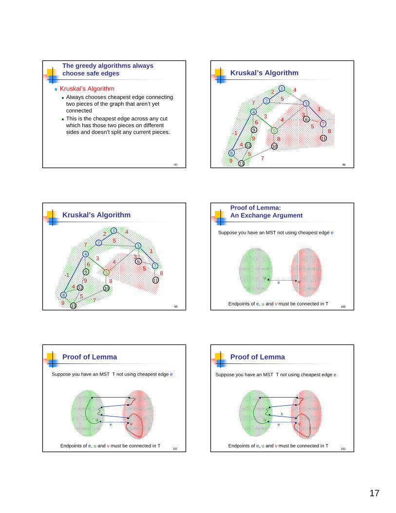
The greedy algorithms always choose safe edges

� Kruskal’s Algorithm� Always chooses cheapest edge connecting

two pieces of the graph that aren’t yet connected

� This is the cheapest edge across any cut which has those two pieces on different sides and doesn’t split any current pieces.

98

Kruskal’s Algorithm

2

7

-1

43

4

5

13

58

6

94

579

8

1

23

10

5

4

9

12

8

13

67

11

99

Kruskal’s Algorithm

2

7

-1

43

4

5

13

58

6

94

579

8

1

23

10

5

4

9

12

8

13

67

11

100

Proof of Lemma:An Exchange Argument

Suppose you have an MST not using cheapest edge e

eu

v

Endpoints of e, u and v must be connected in T

101

Proof of Lemma

Suppose you have an MST T not using cheapest edge e

eu

v

Endpoints of e, u and v must be connected in T102

Proof of Lemma

Suppose you have an MST T not using cheapest edge e

eu

v


h

18

103

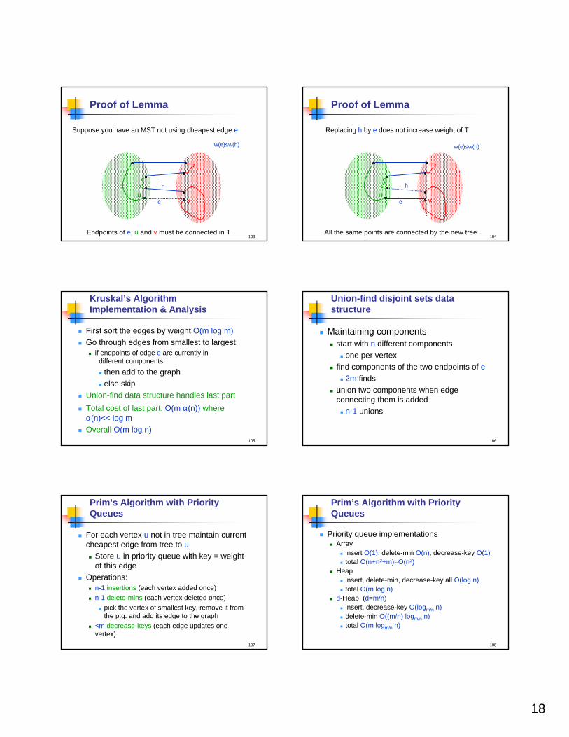
Proof of Lemma

Suppose you have an MST not using cheapest edge e

eu

v


w(e)≤w(h)

h

104

Proof of Lemma

Replacing h by e does not increase weight of T

eu

v

h

w(e)≤w(h)

All the same points are connected by the new tree

105

Kruskal’s Algorithm Implementation & Analysis

� First sort the edges by weight O(m log m)� Go through edges from smallest to largest

� if endpoints of edge e are currently in different components

� then add to the graph� else skip

� Union-find data structure handles last part

� Total cost of last part: O(m α(n)) whereα(n)<< log m

� Overall O(m log n)106

Union-find disjoint sets data structure

� Maintaining components� start with n different components

� one per vertex� find components of the two endpoints of e

� 2m finds� union two components when edge

connecting them is added� n-1 unions

107

Prim’s Algorithm with Priority Queues

� For each vertex u not in tree maintain current cheapest edge from tree to u� Store u in priority queue with key = weight

of this edge� Operations:

� n-1 insertions (each vertex added once)� n-1 delete-mins (each vertex deleted once)

� pick the vertex of smallest key, remove it from the p.q. and add its edge to the graph

� <m decrease-keys (each edge updates one vertex)

108

Prim’s Algorithm with Priority Queues

� Priority queue implementations� Array

� insert O(1), delete-min O(n), decrease-key O(1)� total O(n+n2+m)=O(n2)

� Heap� insert, delete-min, decrease-key all O(log n)� total O(m log n)

� d-Heap (d=m/n)� insert, decrease-key O(logm/n n)� delete-min O((m/n) logm/n n)� total O(m logm/n n)

19

109

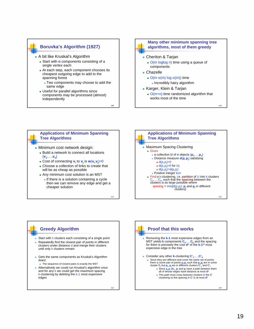
Boruvka’s Algorithm (1927)

� A bit like Kruskal’s Algorithm� Start with n components consisting of a

single vertex each� At each step, each component chooses its

cheapest outgoing edge to add to the spanning forest� Two components may choose to add the

same edge� Useful for parallel algorithms since

components may be processed (almost) independently

110

Many other minimum spanning tree algorithms, most of them greedy

� Cheriton & Tarjan� O(m loglog n) time using a queue of

components

� Chazelle� O(m α(m) log α(m)) time

� Incredibly hairy algorithm

� Karger, Klein & Tarjan� O(m+n) time randomized algorithm that

works most of the time

111

Applications of Minimum Spanning Tree Algorithms

� Minimum cost network design:� Build a network to connect all locations

{v1,…,vn}� Cost of connecting v i to v j is w(v i,v j)>0� Choose a collection of links to create that

will be as cheap as possible� Any minimum cost solution is an MST

� If there is a solution containing a cycle then we can remove any edge and get a cheaper solution

112

Applications of Minimum Spanning Tree Algorithms

� Maximum Spacing Clustering� Given

� a collection U of n objects {p1,…,pn}� Distance measure d(p i,p j) satisfying

� d(pi,pi)=0� d(pi,pj)>0 for i≠j� d(pi,pj)=d(pj,pi)

� Positive integer k≤n� Find a k-clustering, i.e. partition of U into k clusters

C1,…,Ck, such that the spacing between the clusters is as large possible where

spacing = min{d(pi,pj): p i and p j in different clusters}

113

Greedy Algorithm

� Start with n clusters each consisting of a single point� Repeatedly find the closest pair of points in different

clusters under distance d and merge their clusters until only k clusters remain

� Gets the same components as Kruskal’s Algorithm does!� The sequence of closest pairs is exactly the MST

� Alternatively we could run Kruskal’s algorithm once and for any k we could get the maximum spacing k-clustering by deleting the k-1 most expensive edges

114

Proof that this works

� Removing the k-1 most expensive edges from an MST yields k components C1,…,Ck and the spacing for them is precisely the cost d* of the k-1st most expensive edge in the tree

� Consider any other k-clustering C’1,…,C’k� Since they are different and cover the same set of points

there is some pair of points p i,p j such that p i,p j are in some cluster Cr but p i, p j are in different clusters C’s and C’ t

� Since p i,p j ∈∈∈∈Cr, p i and p j have a path between them all of whose edges have distance at most d*

� This path must cross between clusters in the C’clustering so the spacing in C’ is at most d*

cse 421: introduction to algorithms - university of washington · cse 421: introduction to...

Documents