CSE 421: Introduction

to Algorithms

Graph

Yin-Tat Lee

1

Trees and Induction

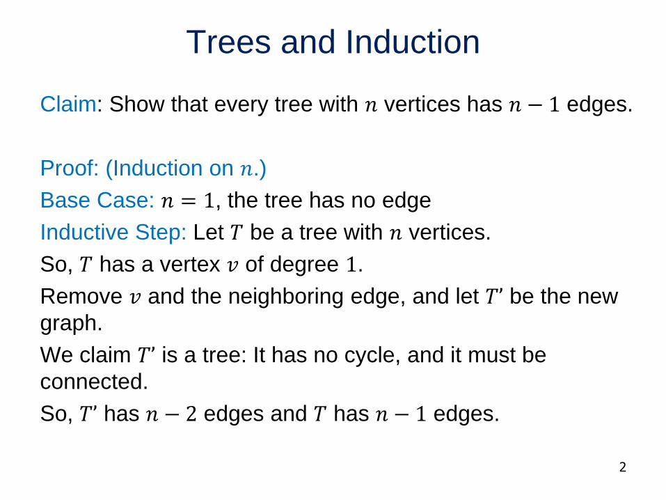
Claim: Show that every tree with 𝑛 vertices has 𝑛 − 1 edges.

Proof: (Induction on 𝑛.)

Base Case: 𝑛 = 1, the tree has no edge

Inductive Step: Let 𝑇 be a tree with 𝑛 vertices.

So, 𝑇 has a vertex 𝑣 of degree 1.

Remove 𝑣 and the neighboring edge, and let 𝑇’ be the new

graph.

We claim 𝑇’ is a tree: It has no cycle, and it must be

connected.

So, 𝑇’ has 𝑛 − 2 edges and 𝑇 has 𝑛 − 1 edges.

2

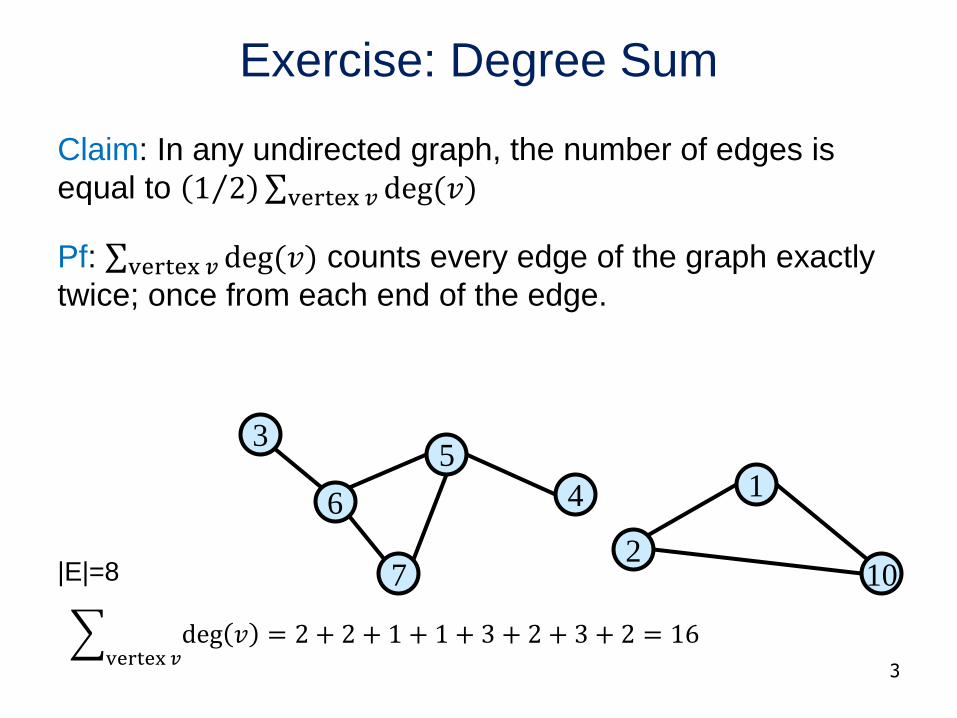
Exercise: Degree Sum

Claim: In any undirected graph, the number of edges is

equal to Τ1 2 σvertex 𝑣 deg(𝑣)

Pf: σvertex 𝑣 deg(𝑣) counts every edge of the graph exactly

twice; once from each end of the edge.

3

3

4

5

6

72

10

1

|E|=8

vertex 𝑣

deg 𝑣 = 2 + 2 + 1 + 1 + 3 + 2 + 3 + 2 = 16

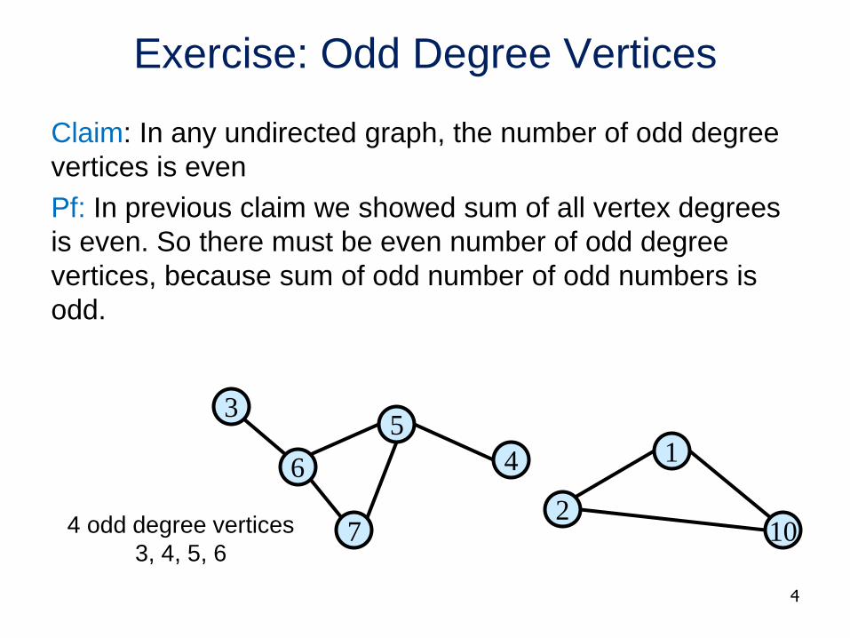
Exercise: Odd Degree Vertices

Claim: In any undirected graph, the number of odd degree

vertices is even

Pf: In previous claim we showed sum of all vertex degrees

is even. So there must be even number of odd degree

vertices, because sum of odd number of odd numbers is

odd.

4

3

4

5

6

72

10

1

4 odd degree vertices

3, 4, 5, 6

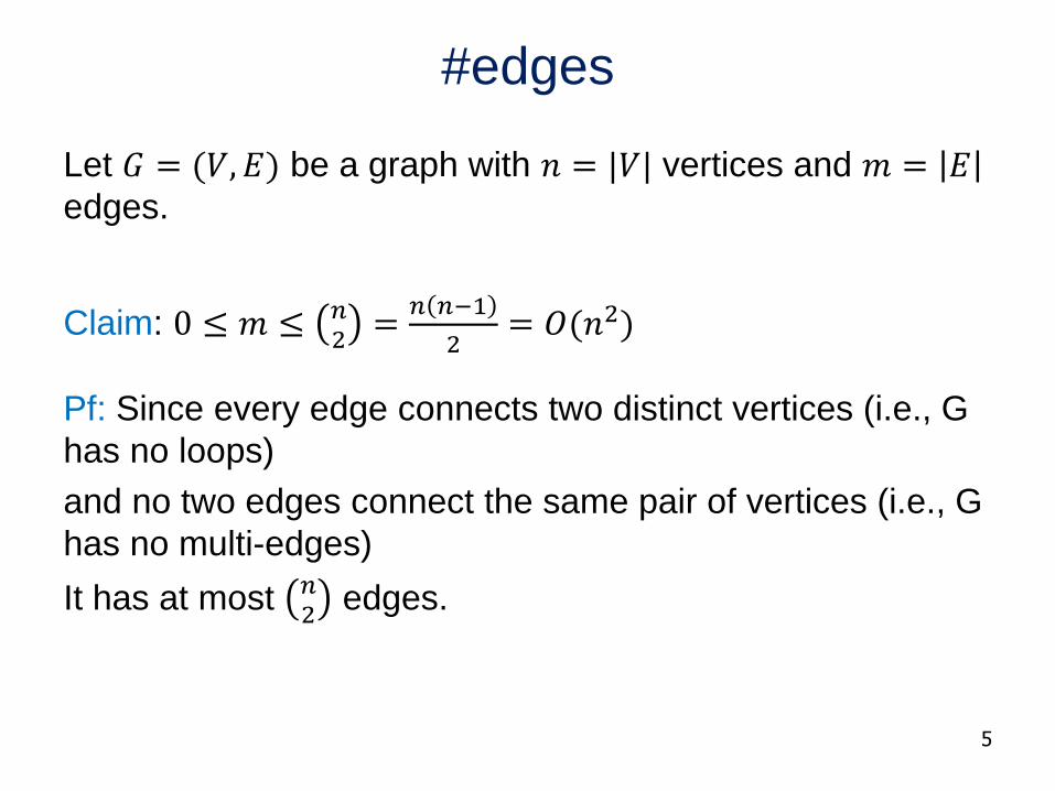
#edges

Let 𝐺 = (𝑉, 𝐸) be a graph with 𝑛 = |𝑉| vertices and 𝑚 = 𝐸edges.

Claim: 0 ≤ 𝑚 ≤ 𝑛2

=𝑛 𝑛−1

2= 𝑂(𝑛2)

Pf: Since every edge connects two distinct vertices (i.e., G

has no loops)

and no two edges connect the same pair of vertices (i.e., G

has no multi-edges)

It has at most 𝑛2

edges.

5

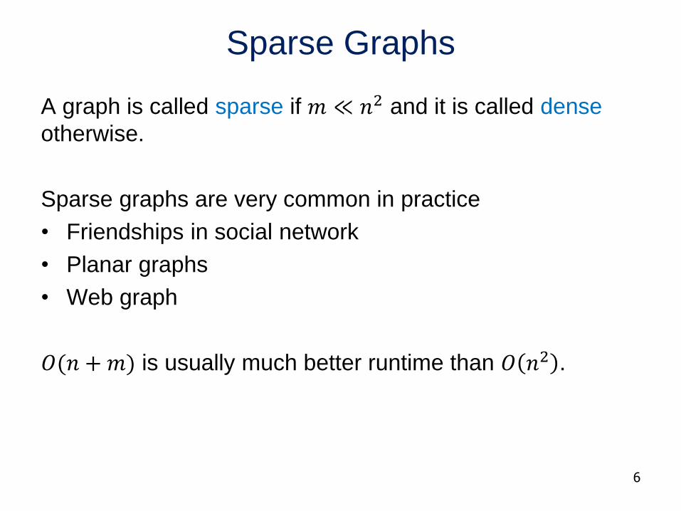
Sparse Graphs

A graph is called sparse if 𝑚 ≪ 𝑛2 and it is called dense

otherwise.

Sparse graphs are very common in practice

• Friendships in social network

• Planar graphs

• Web graph

𝑂(𝑛 +𝑚) is usually much better runtime than 𝑂 𝑛2 .

6

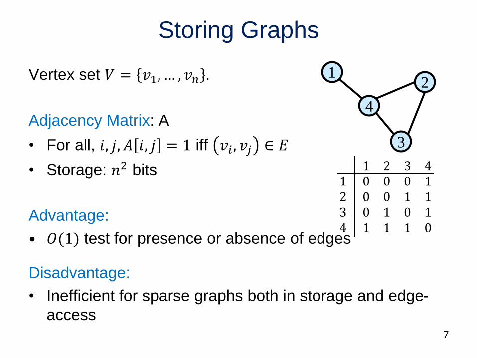
Storing Graphs

Vertex set 𝑉 = 𝑣1, … , 𝑣𝑛 .

Adjacency Matrix: A

• For all, 𝑖, 𝑗, 𝐴 𝑖, 𝑗 = 1 iff 𝑣𝑖 , 𝑣𝑗 ∈ 𝐸

• Storage: 𝑛2 bits

Advantage:

• 𝑂(1) test for presence or absence of edges

Disadvantage:

• Inefficient for sparse graphs both in storage and edge-

access7

12

4

3

1 2 3 41 0 0 0 12 0 0 1 13 0 1 0 14 1 1 1 0

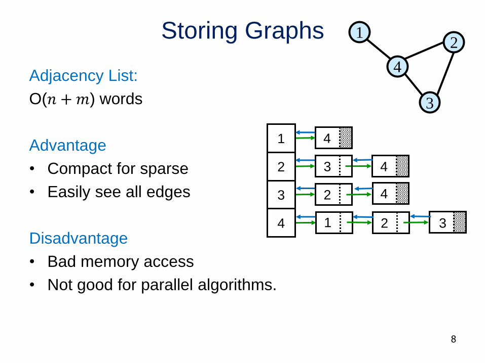
Storing Graphs

Adjacency List:

O(𝑛 +𝑚) words

Advantage

• Compact for sparse

• Easily see all edges

Disadvantage

• Bad memory access

• Not good for parallel algorithms.

8

12

4

3

4

3

3

2

1

4

2 4

1 2

43

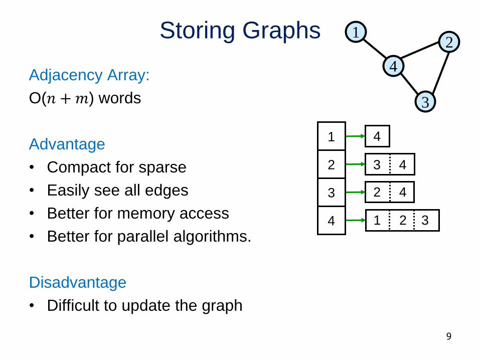
Storing Graphs

Adjacency Array:

O(𝑛 +𝑚) words

Advantage

• Compact for sparse

• Easily see all edges

• Better for memory access

• Better for parallel algorithms.

Disadvantage

• Difficult to update the graph

9

12

4

3

4

3

2

1

4

2 4

1 2 3

3 4

Storing Graphs

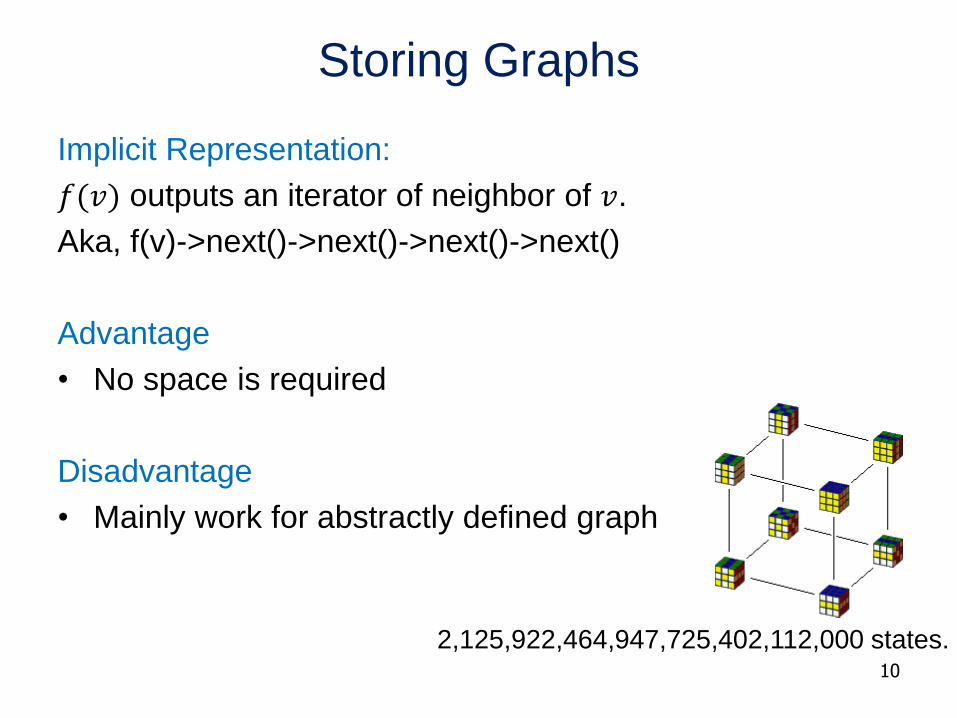
Implicit Representation:

𝑓(𝑣) outputs an iterator of neighbor of 𝑣.

Aka, f(v)->next()->next()->next()->next()

Advantage

• No space is required

Disadvantage

• Mainly work for abstractly defined graph

10

2,125,922,464,947,725,402,112,000 states.

CSE 421: Introduction

to Algorithms

Breadth First Search

Yin Tat Lee

11

Graph Traversal

Walk (via edges) from a fixed starting vertex 𝑠 to all vertices

reachable from 𝑠.

Applications:

• Web crawling

• Social networking

• Network Broadcasting

• Garbage Collection

• …

12

https://idea-instructions.com/

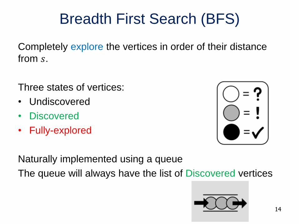
Breadth First Search (BFS)

Completely explore the vertices in order of their distance

from 𝑠.

Three states of vertices:

• Undiscovered

• Discovered

• Fully-explored

Naturally implemented using a queue

The queue will always have the list of Discovered vertices

14

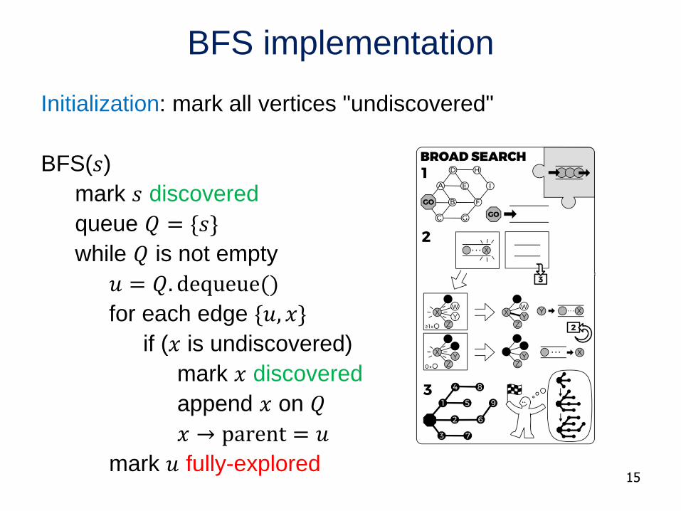
BFS implementation

Initialization: mark all vertices "undiscovered"

BFS(𝑠)

mark 𝑠 discovered

queue 𝑄 = {𝑠}

while 𝑄 is not empty

𝑢 = 𝑄. dequeue()

for each edge {𝑢, 𝑥}

if (𝑥 is undiscovered)

mark 𝑥 discovered

append 𝑥 on 𝑄

𝑥 → parent = 𝑢

mark 𝑢 fully-explored15

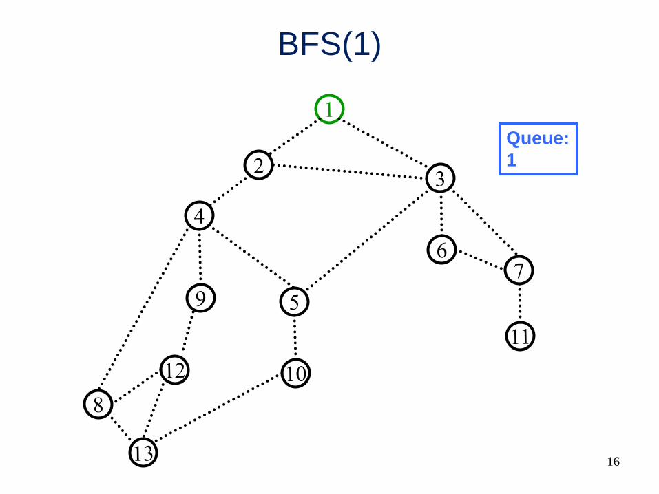
16

BFS(1)

Queue:

1

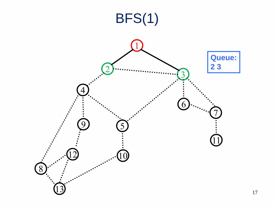
17

BFS(1)

Queue:

2 3

18

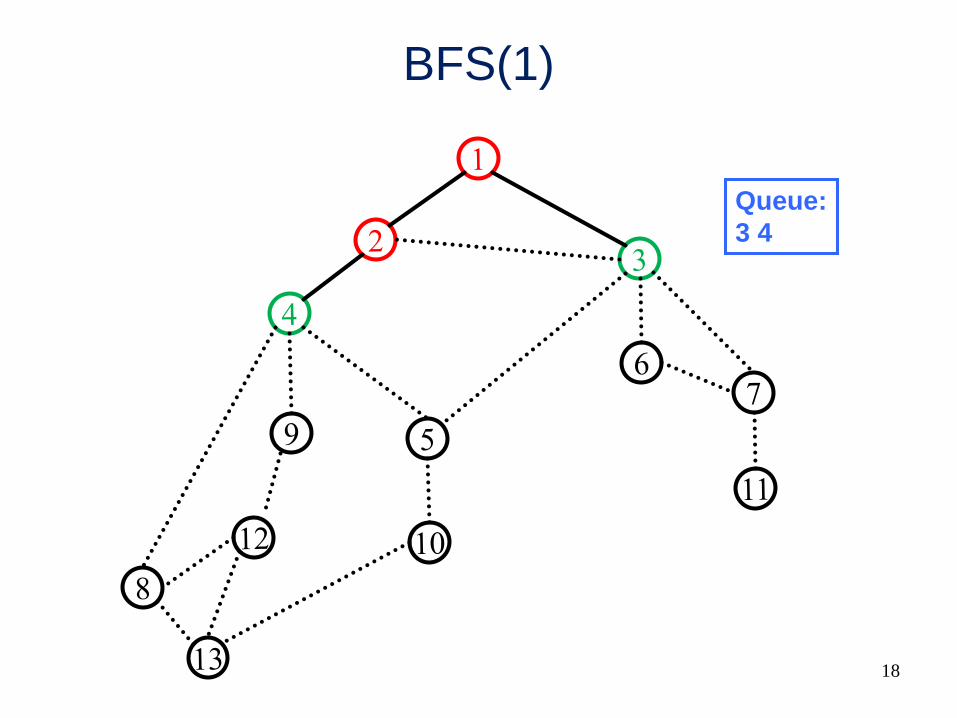
BFS(1)

Queue:

3 4

19

BFS(1)

Queue:

4 5 6 7

20

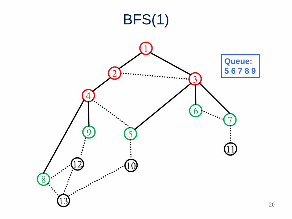
BFS(1)

Queue:

5 6 7 8 9

21

BFS(1)

Queue:

7 8 9 10

22

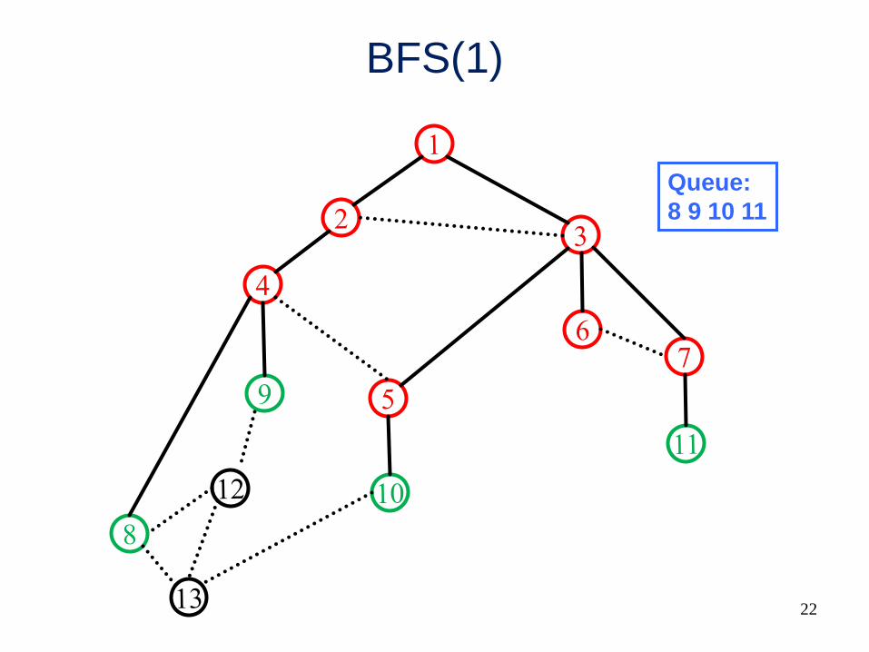
BFS(1)

Queue:

8 9 10 11

23

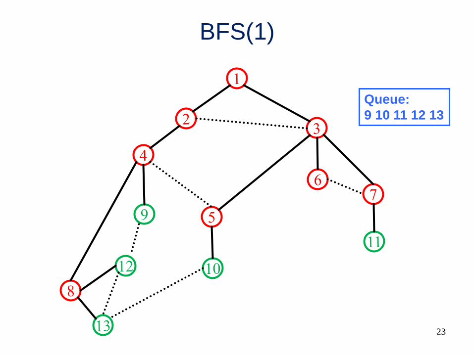
BFS(1)

Queue:

9 10 11 12 13

24

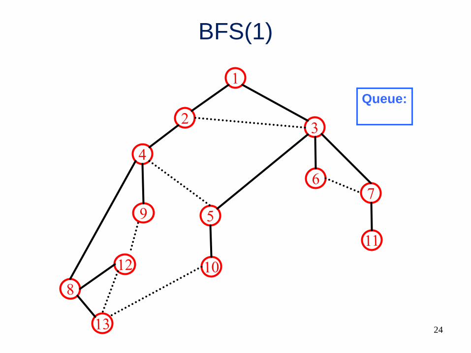
BFS(1)

Queue:

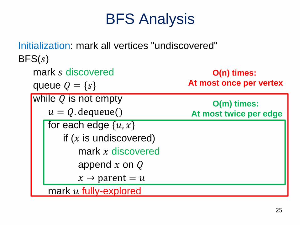
BFS Analysis

Initialization: mark all vertices "undiscovered"

BFS(𝑠)

mark 𝑠 discovered

queue 𝑄 = {𝑠}

while 𝑄 is not empty

𝑢 = 𝑄. dequeue()

for each edge {𝑢, 𝑥}

if (𝑥 is undiscovered)

mark 𝑥 discovered

append 𝑥 on 𝑄

𝑥 → parent = 𝑢

mark 𝑢 fully-explored

25

O(m) times:

At most twice per edge

O(n) times:

At most once per vertex

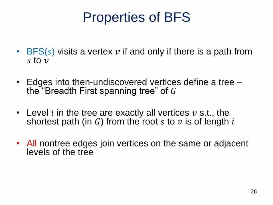
Properties of BFS

• BFS(𝑠) visits a vertex 𝑣 if and only if there is a path from 𝑠 to 𝑣

• Edges into then-undiscovered vertices define a tree –the “Breadth First spanning tree” of 𝐺

• Level 𝑖 in the tree are exactly all vertices 𝑣 s.t., the shortest path (in 𝐺) from the root 𝑠 to 𝑣 is of length 𝑖

• All nontree edges join vertices on the same or adjacent levels of the tree

26

27

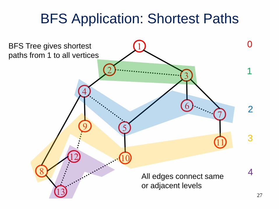
BFS Application: Shortest Paths

BFS Tree gives shortest

paths from 1 to all vertices

0

1

2

3

4All edges connect same

or adjacent levels

28

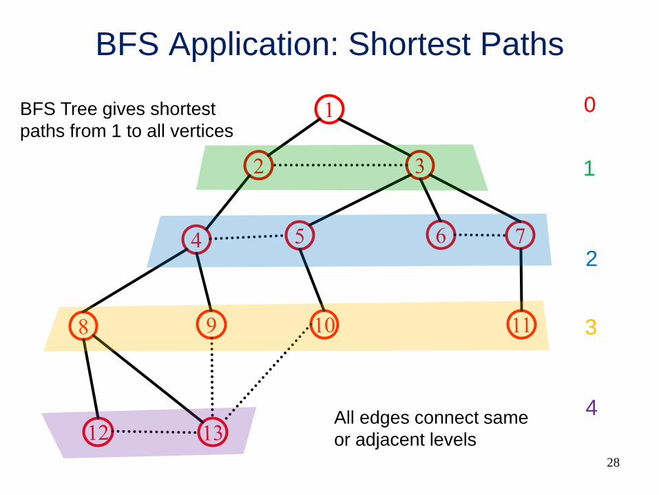
BFS Application: Shortest Paths

BFS Tree gives shortest

paths from 1 to all vertices

0

1

2

3

4All edges connect same

or adjacent levels

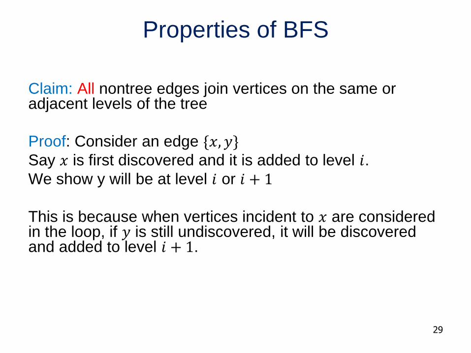
Properties of BFS

Claim: All nontree edges join vertices on the same or adjacent levels of the tree

Proof: Consider an edge {𝑥, 𝑦}Say 𝑥 is first discovered and it is added to level 𝑖.We show y will be at level 𝑖 or 𝑖 + 1

This is because when vertices incident to 𝑥 are considered in the loop, if 𝑦 is still undiscovered, it will be discovered and added to level 𝑖 + 1.

29

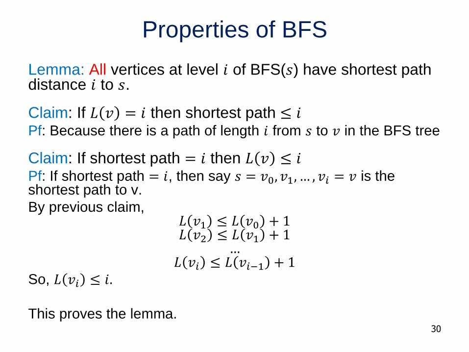
Properties of BFS

Lemma: All vertices at level 𝑖 of BFS(𝑠) have shortest path distance 𝑖 to 𝑠.

Claim: If 𝐿 𝑣 = 𝑖 then shortest path ≤ 𝑖Pf: Because there is a path of length 𝑖 from 𝑠 to 𝑣 in the BFS tree

Claim: If shortest path = 𝑖 then 𝐿 𝑣 ≤ 𝑖Pf: If shortest path = 𝑖, then say 𝑠 = 𝑣0, 𝑣1, … , 𝑣𝑖 = 𝑣 is the shortest path to v.

By previous claim, 𝐿 𝑣1 ≤ 𝐿 𝑣0 + 1𝐿 𝑣2 ≤ 𝐿 𝑣1 + 1

…𝐿 𝑣𝑖 ≤ 𝐿 𝑣𝑖−1 + 1

So, 𝐿 𝑣𝑖 ≤ 𝑖.

This proves the lemma. 30

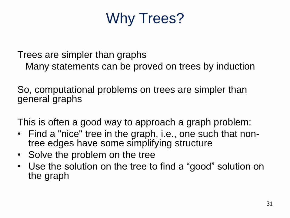
Why Trees?

Trees are simpler than graphs

Many statements can be proved on trees by induction

So, computational problems on trees are simpler than general graphs

This is often a good way to approach a graph problem:

• Find a "nice" tree in the graph, i.e., one such that non-tree edges have some simplifying structure

• Solve the problem on the tree

• Use the solution on the tree to find a “good” solution on the graph

31

CSE 421: Introduction

to Algorithms

Application of BFS

Yin Tat Lee

32

BFS Application: Connected Component

We want to answer the following type questions (fast):

Given vertices 𝑢, 𝑣 is there a path from 𝑢 to 𝑣 in 𝐺?

Idea: Create an array 𝐴 such that

For all 𝑢 in the same connected component, 𝐴[𝑢] is same.

Therefore, question reduces to

If A[u] = A[v]?

33

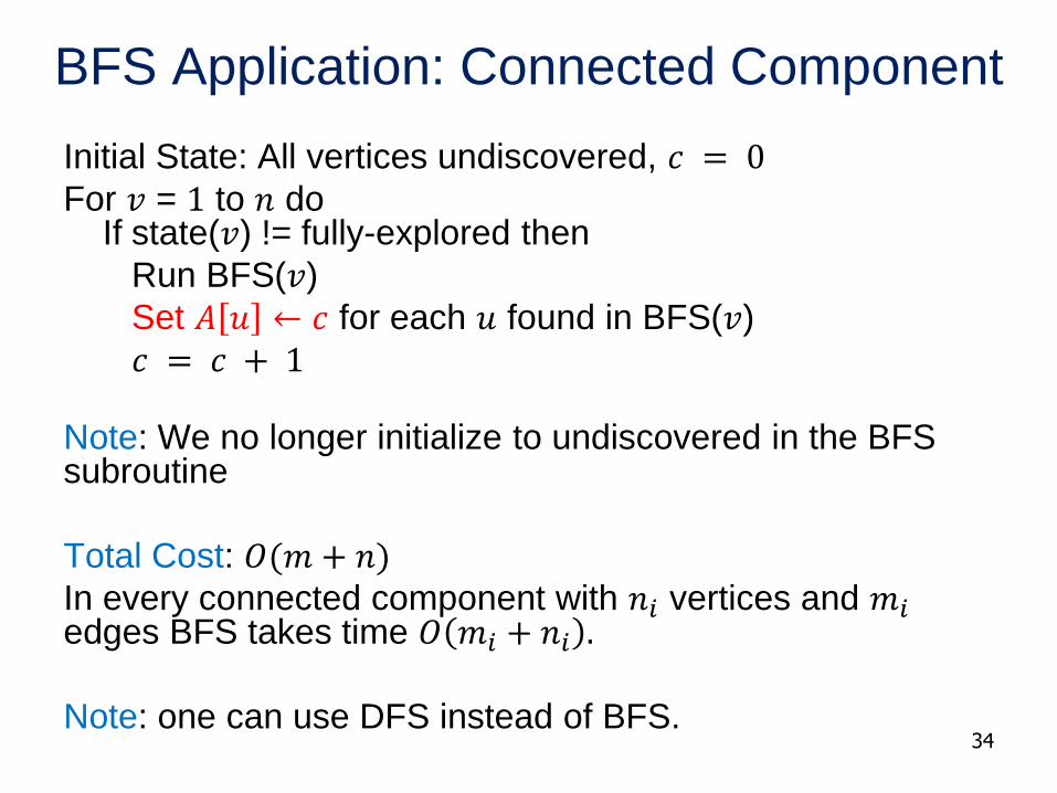
Initial State: All vertices undiscovered, 𝑐 = 0For 𝑣 = 1 to 𝑛 do

If state(𝑣) != fully-explored then

Run BFS(𝑣)

Set 𝐴 𝑢 ← 𝑐 for each 𝑢 found in BFS(𝑣)

𝑐 = 𝑐 + 1

Note: We no longer initialize to undiscovered in the BFS subroutine

Total Cost: 𝑂(𝑚 + 𝑛)In every connected component with 𝑛𝑖 vertices and 𝑚𝑖edges BFS takes time 𝑂 𝑚𝑖 + 𝑛𝑖 .

Note: one can use DFS instead of BFS.34

BFS Application: Connected Component

Connected Components

Lesson: We can execute any algorithm on disconnected graphs by running it on each connected component.

We can use the previous algorithm to detect connected components.

There is no overhead, because the algorithm runs in time 𝑂(𝑚 + 𝑛).

So, from now on, we can (almost) always assume the input graph is connected.

35

Cycles in Graphs

Claim: If an 𝑛 vertices graph 𝐺 has at least 𝑛 edges, then it has a cycle.

Proof: If 𝐺 is connected, then it cannot be a tree. Because every tree has 𝑛 − 1 edges. So, it has a cycle.

Suppose 𝐺 is disconnected. Say connected components of G have 𝑛1, … , 𝑛𝑘vertices where 𝑛1 +⋯+ 𝑛𝑘 = 𝑛

Since 𝐺 has ≥ 𝑛 edges, there must be some 𝑖 such that a component has 𝑛𝑖 vertices with at least 𝑛𝑖 edges.

Therefore, in that component we do not have a tree, so there is a cycle.

36

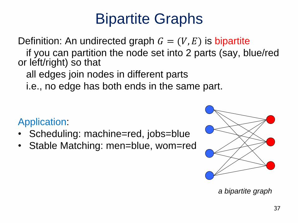
Bipartite Graphs

Definition: An undirected graph 𝐺 = (𝑉, 𝐸) is bipartite

if you can partition the node set into 2 parts (say, blue/red or left/right) so that

all edges join nodes in different parts

i.e., no edge has both ends in the same part.

Application:

• Scheduling: machine=red, jobs=blue

• Stable Matching: men=blue, wom=red

37

a bipartite graph

Testing Bipartiteness

Problem: Given a graph 𝐺, is it bipartite?

Many graph problems become:

• Easier/Tractable if the underlying graph is bipartite (matching)

Before attempting to design an algorithm, we need to

understand structure of bipartite graphs.

38

v1

v2 v3

v6 v5 v4

v7

v2

v4

v5

v7

v1

v3

v6

a bipartite graph G another drawing of G

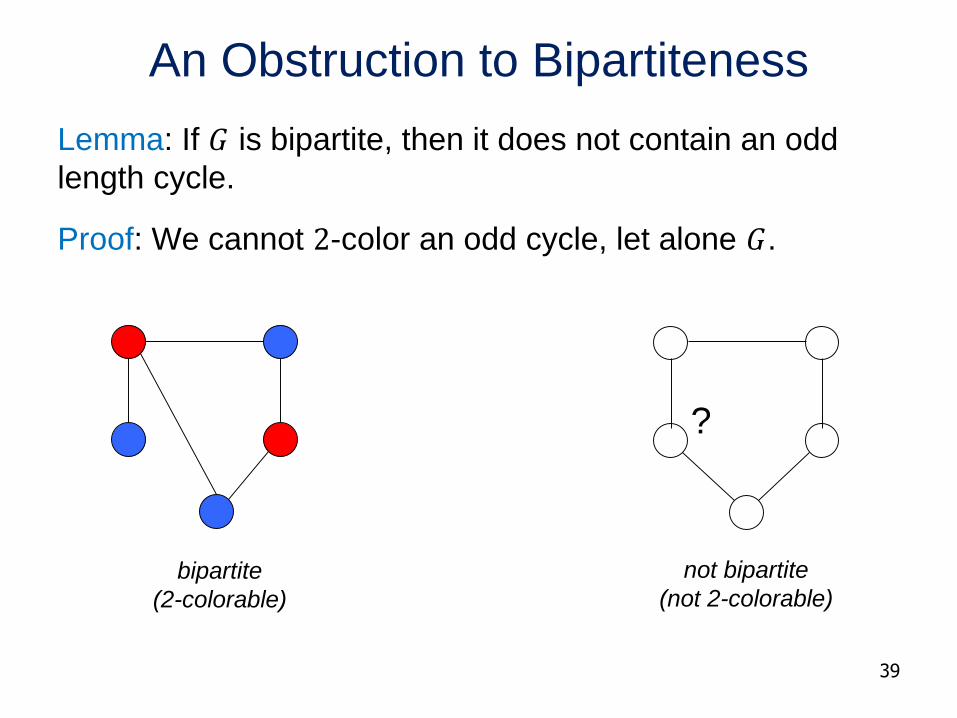
An Obstruction to Bipartiteness

Lemma: If 𝐺 is bipartite, then it does not contain an odd

length cycle.

Proof: We cannot 2-color an odd cycle, let alone 𝐺.

39

bipartite

(2-colorable)

not bipartite

(not 2-colorable)

?

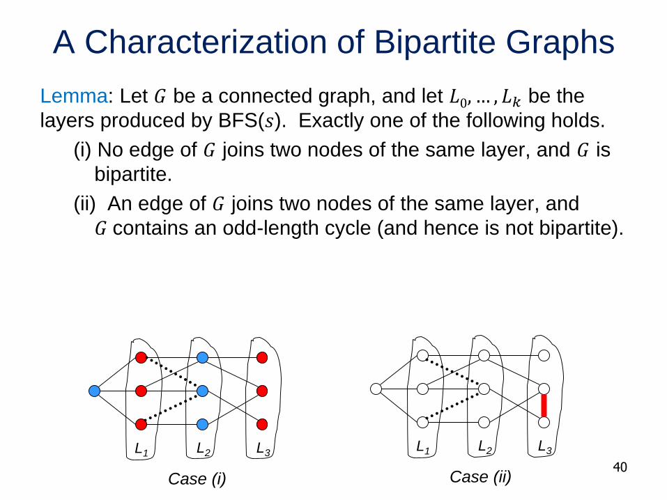
A Characterization of Bipartite Graphs

Lemma: Let 𝐺 be a connected graph, and let 𝐿0, … , 𝐿𝑘 be the

layers produced by BFS(𝑠). Exactly one of the following holds.

(i) No edge of 𝐺 joins two nodes of the same layer, and 𝐺 is

bipartite.

(ii) An edge of 𝐺 joins two nodes of the same layer, and

𝐺 contains an odd-length cycle (and hence is not bipartite).

40Case (i)

L1 L2 L3

Case (ii)

L1 L2 L3

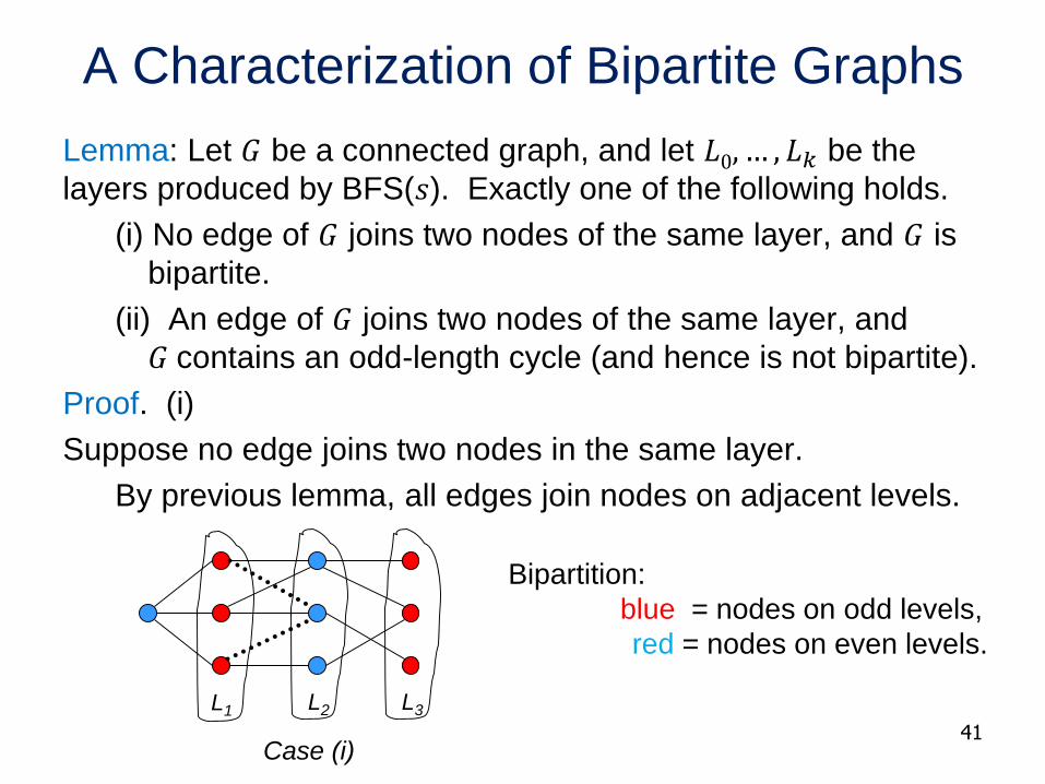
A Characterization of Bipartite Graphs

Lemma: Let 𝐺 be a connected graph, and let 𝐿0, … , 𝐿𝑘 be the

layers produced by BFS(𝑠). Exactly one of the following holds.

(i) No edge of 𝐺 joins two nodes of the same layer, and 𝐺 is

bipartite.

(ii) An edge of 𝐺 joins two nodes of the same layer, and

𝐺 contains an odd-length cycle (and hence is not bipartite).

Proof. (i)

Suppose no edge joins two nodes in the same layer.

By previous lemma, all edges join nodes on adjacent levels.

41Case (i)

L1 L2 L3

Bipartition:

blue = nodes on odd levels,

red = nodes on even levels.

A Characterization of Bipartite Graphs

Lemma: Let 𝐺 be a connected graph, and let 𝐿0, … , 𝐿𝑘 be the

layers produced by BFS(𝑠). Exactly one of the following holds.

(i) No edge of 𝐺 joins two nodes of the same layer, and 𝐺 is

bipartite.

(ii) An edge of 𝐺 joins two nodes of the same layer, and

𝐺 contains an odd-length cycle (and hence is not bipartite).

Proof. (ii)

Suppose {𝑥, 𝑦} is an edge & 𝑥, 𝑦 in same level 𝐿𝑗.

Let 𝑧 = their lowest common ancestor in BFS tree.

Let 𝐿𝑖 be level containing 𝑧.

Consider cycle that takes edge from 𝑥 to 𝑦,

then tree from 𝑦 to 𝑧, then tree from 𝑧 to 𝑥.

Its length is 1 + 𝑗 − 𝑖 + (𝑗 − 𝑖), which is odd.

42

z = lca(x, y)

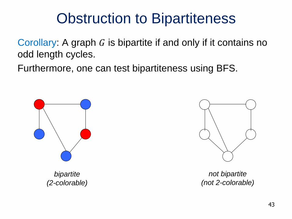
Obstruction to Bipartiteness

Corollary: A graph 𝐺 is bipartite if and only if it contains no

odd length cycles.

Furthermore, one can test bipartiteness using BFS.

43

bipartite

(2-colorable)

not bipartite

(not 2-colorable)