CSE 421Algorithms

Richard Anderson

Lecture 13

Divide and Conquer

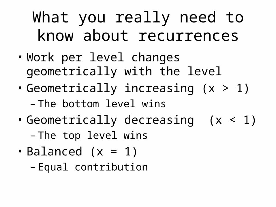
What you really need to know about recurrences

• Work per level changes geometrically with the level

• Geometrically increasing (x > 1)– The bottom level wins

• Geometrically decreasing (x < 1)– The top level wins

• Balanced (x = 1)– Equal contribution

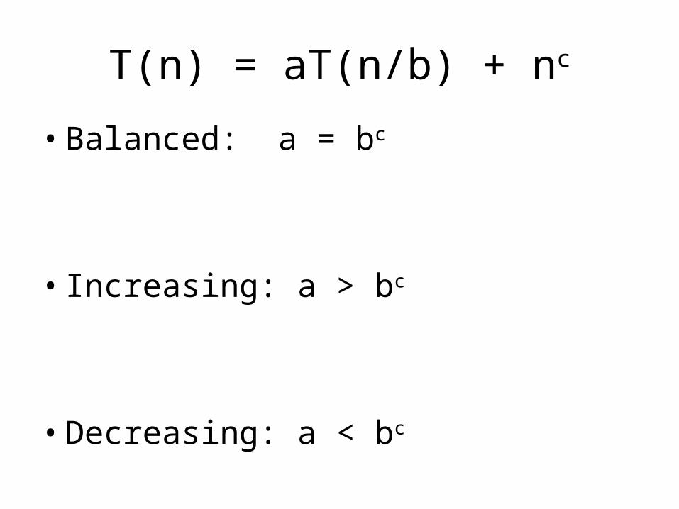
T(n) = aT(n/b) + nc

• Balanced: a = bc

• Increasing: a > bc

• Decreasing: a < bc

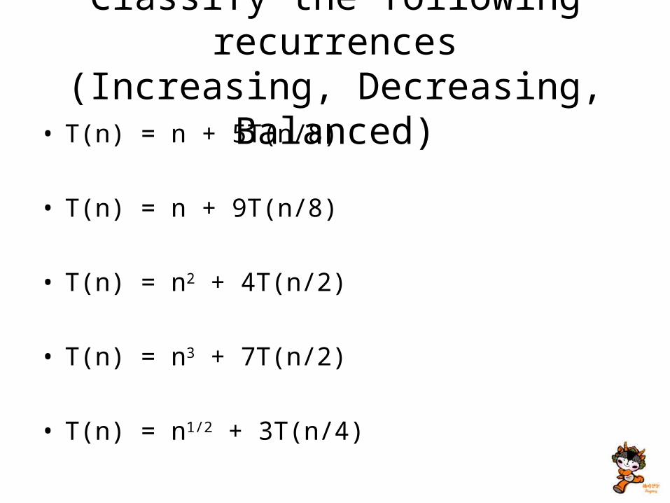
Classify the following recurrences(Increasing, Decreasing, Balanced)• T(n) = n + 5T(n/8)

• T(n) = n + 9T(n/8)

• T(n) = n2 + 4T(n/2)

• T(n) = n3 + 7T(n/2)

• T(n) = n1/2 + 3T(n/4)

Divide and Conquer Algorithms

• Split into sub problems• Recursively solve the problem• Combine solutions

• Make progress in the split and combine stages– Quicksort – progress made at the split step– Mergesort – progress made at the combine

step

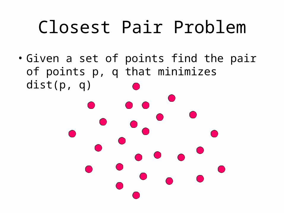
Closest Pair Problem

• Given a set of points find the pair of points p, q that minimizes dist(p, q)

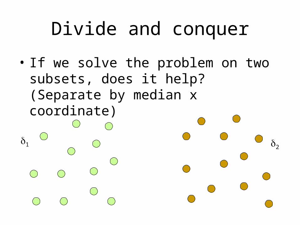
Divide and conquer

• If we solve the problem on two subsets, does it help? (Separate by median x coordinate)

1 2

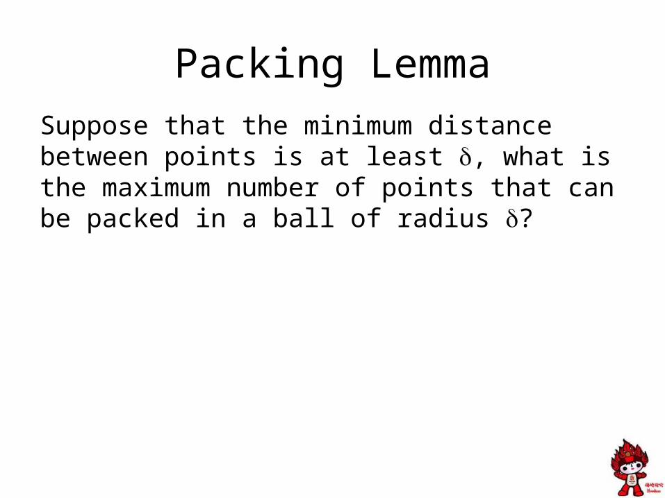
Packing Lemma

Suppose that the minimum distance between points is at least , what is the maximum number of points that can be packed in a ball of radius ?

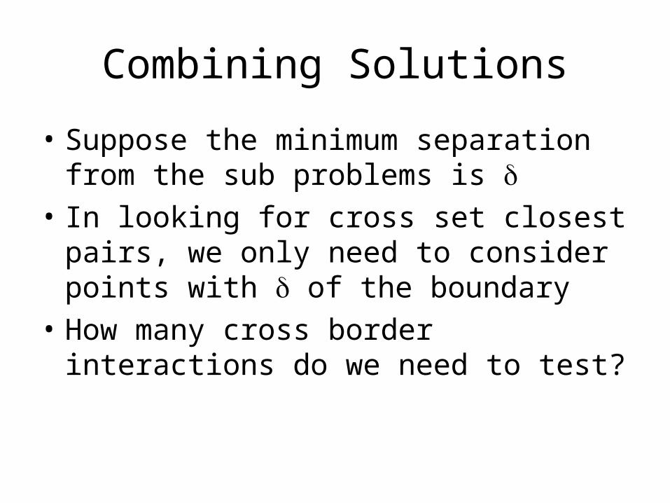
Combining Solutions

• Suppose the minimum separation from the sub problems is

• In looking for cross set closest pairs, we only need to consider points with of the boundary

• How many cross border interactions do we need to test?

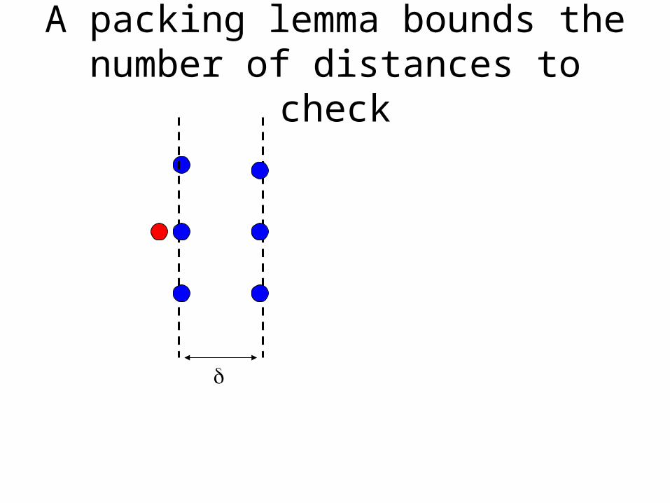
A packing lemma bounds the number of distances to check

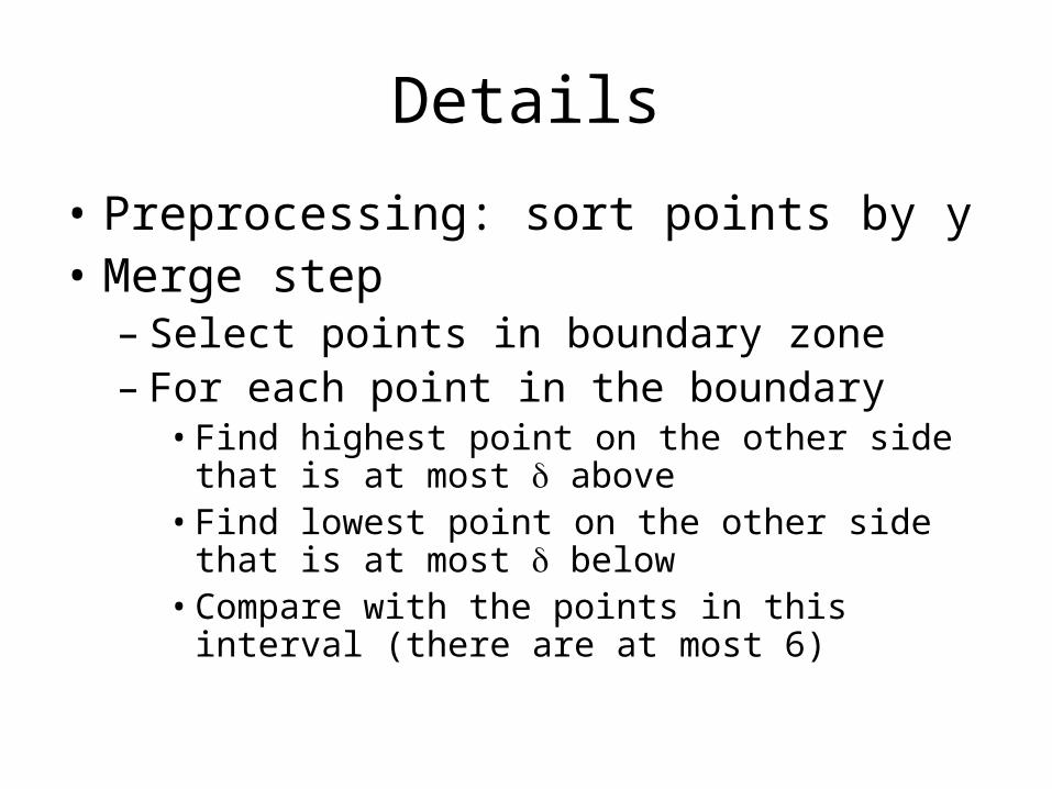
Details

• Preprocessing: sort points by y• Merge step

– Select points in boundary zone– For each point in the boundary

• Find highest point on the other side that is at most above

• Find lowest point on the other side that is at most below

• Compare with the points in this interval (there are at most 6)

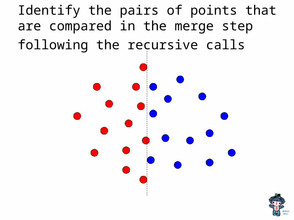
Identify the pairs of points that are compared in the merge step following the recursive

calls

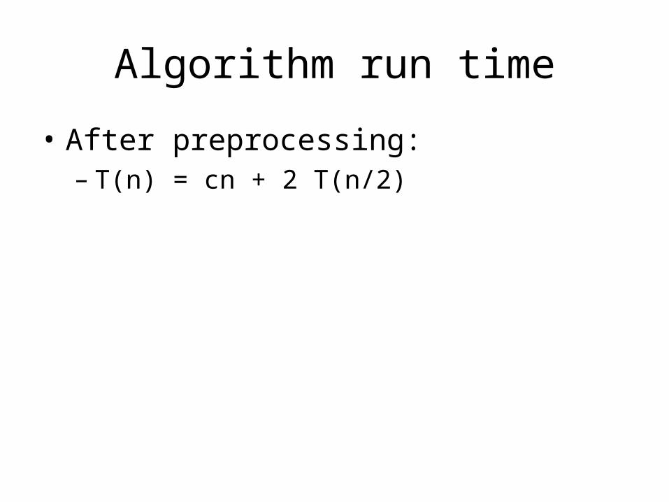
Algorithm run time

• After preprocessing:– T(n) = cn + 2 T(n/2)

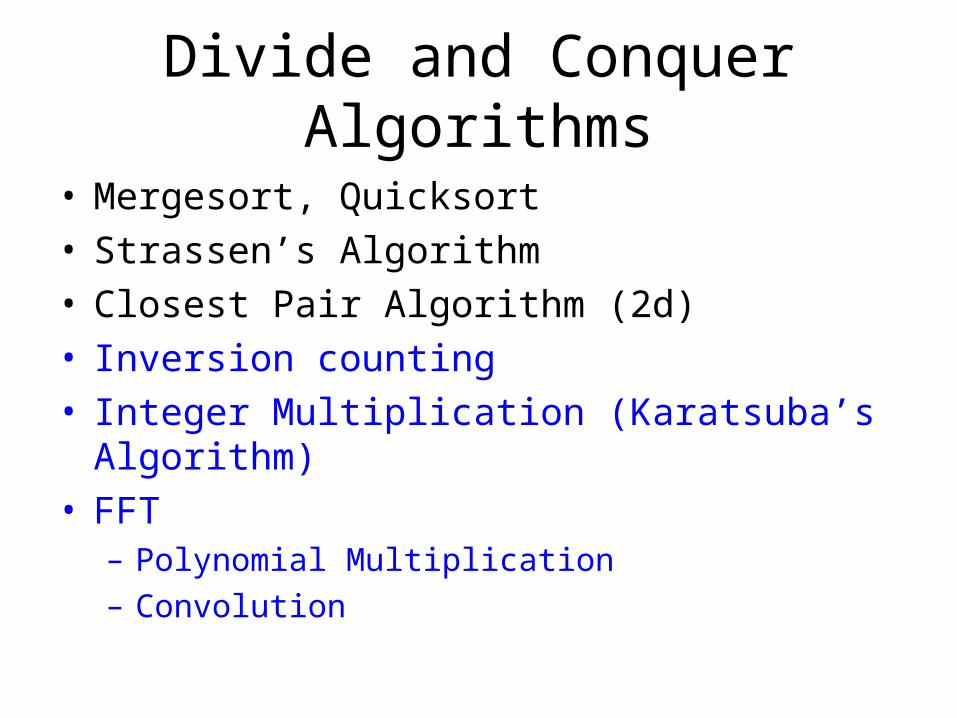
Divide and Conquer Algorithms

• Mergesort, Quicksort• Strassen’s Algorithm• Closest Pair Algorithm (2d)• Inversion counting• Integer Multiplication (Karatsuba’s Algorithm)• FFT

– Polynomial Multiplication– Convolution

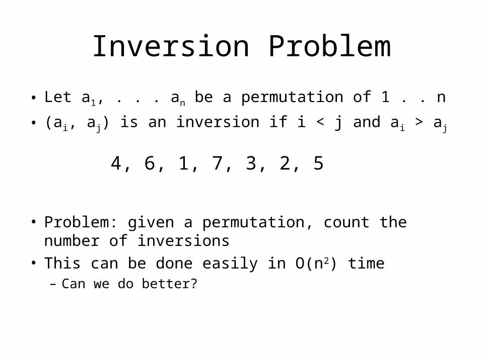
Inversion Problem

• Let a1, . . . an be a permutation of 1 . . n

• (ai, aj) is an inversion if i < j and ai > aj

• Problem: given a permutation, count the number of inversions

• This can be done easily in O(n2) time– Can we do better?

4, 6, 1, 7, 3, 2, 5

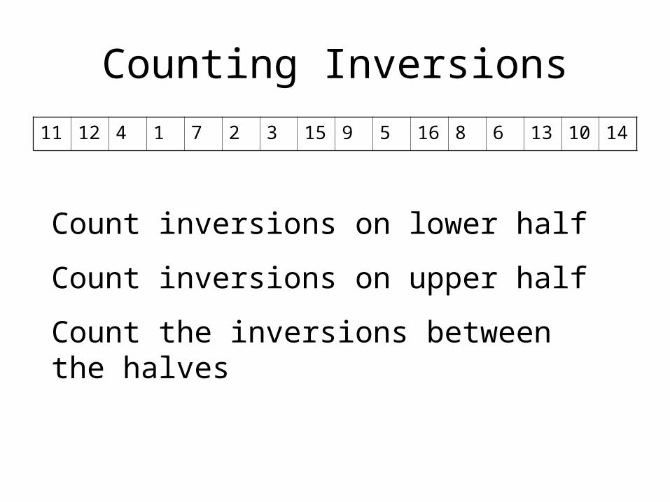
Counting Inversions

11 12 4 1 7 2 3 15 9 5 16 8 6 13 10 14

Count inversions on lower half

Count inversions on upper half

Count the inversions between the halves

11 12 4 1 7 2 3 15

11 12 4 1 7 2 3 15

9 5 16 8 6 13 10 14

9 5 16 8 6 13 10 14

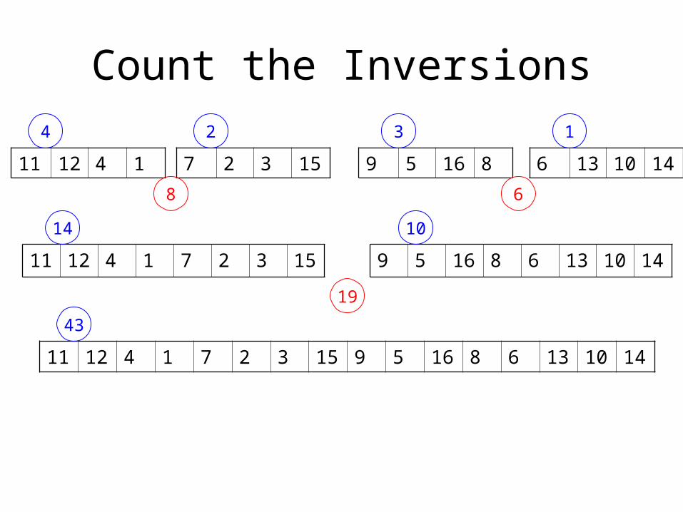
Count the Inversions

11 12 4 1 7 2 3 15 9 5 16 8 6 13 10 14

4 12 3

14 10

19

8 6

43

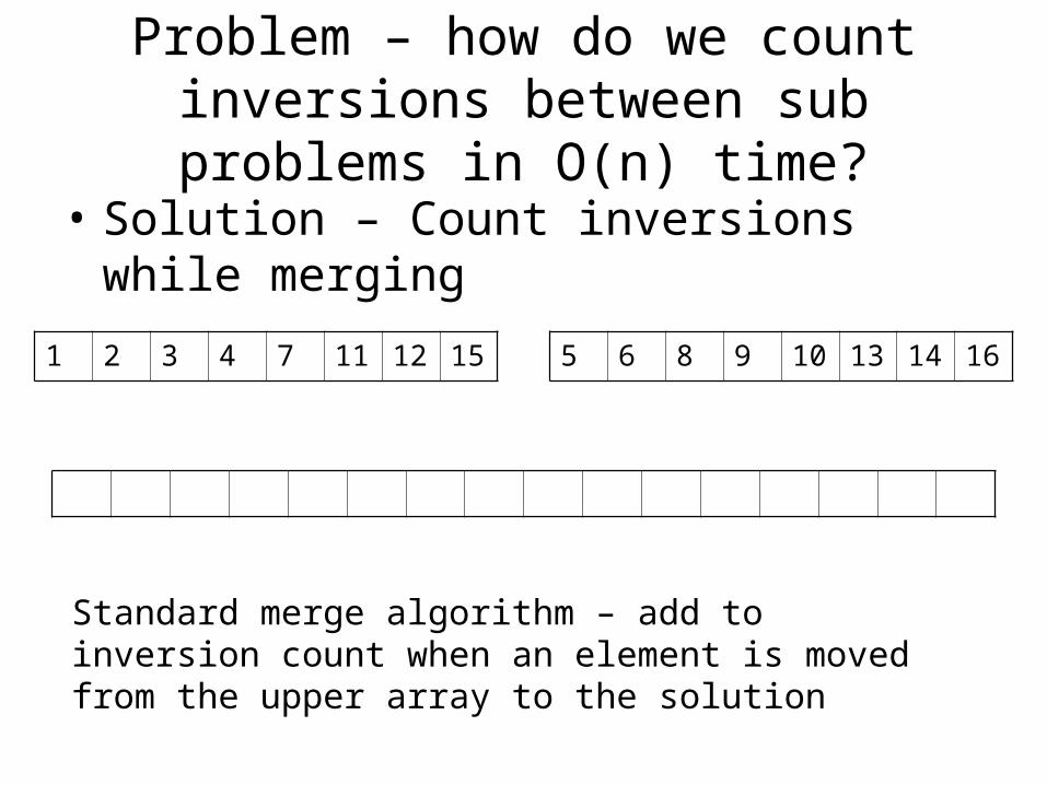
Problem – how do we count inversions between sub problems in O(n) time?

• Solution – Count inversions while merging

1 2 3 4 7 11 12 15 5 6 8 9 10 13 14 16

Standard merge algorithm – add to inversion count when an element is moved from the upper array to the solution

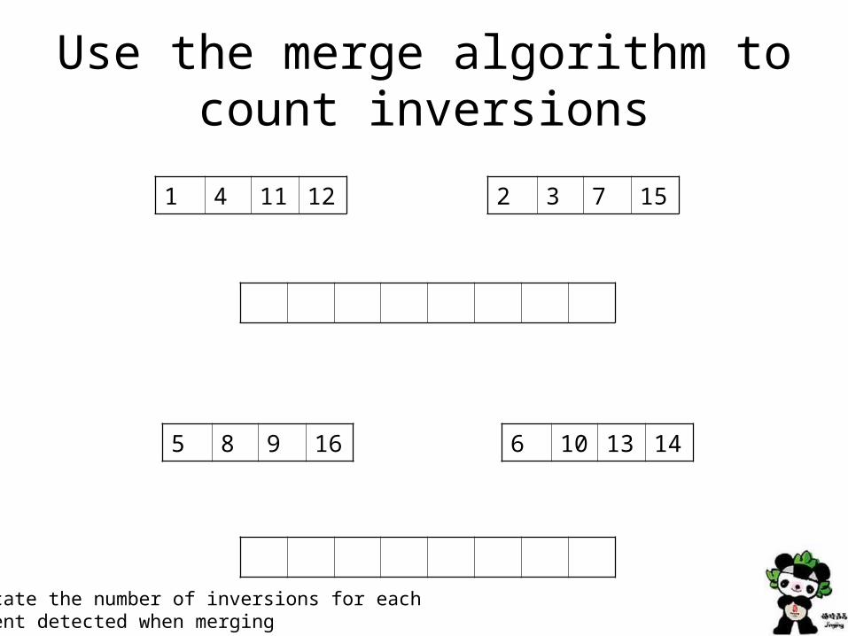
Use the merge algorithm to count inversions

1 4 11 12 2 3 7 15

5 8 9 16 6 10 13 14

Indicate the number of inversions for eachelement detected when merging

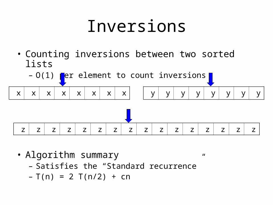
Inversions

• Counting inversions between two sorted lists– O(1) per element to count inversions

• Algorithm summary– Satisfies the “Standard recurrence” – T(n) = 2 T(n/2) + cn

x x x x x x x x y y y y y y y y

z z z z z z z z z z z z z z z z

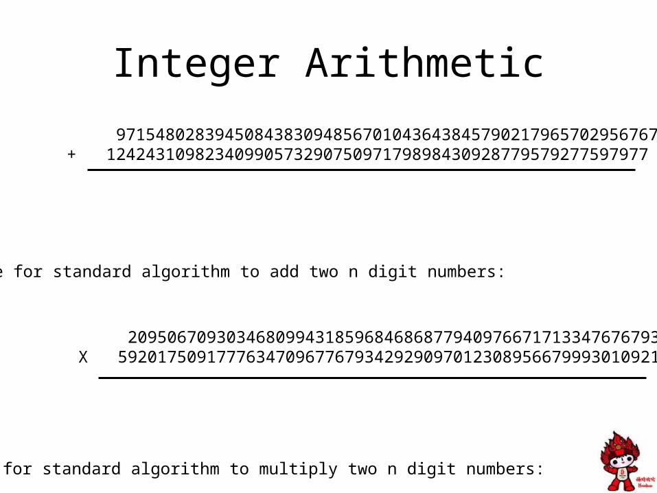
Integer Arithmetic

9715480283945084383094856701043643845790217965702956767+ 1242431098234099057329075097179898430928779579277597977

2095067093034680994318596846868779409766717133476767930X 5920175091777634709677679342929097012308956679993010921

Runtime for standard algorithm to add two n digit numbers:

Runtime for standard algorithm to multiply two n digit numbers:

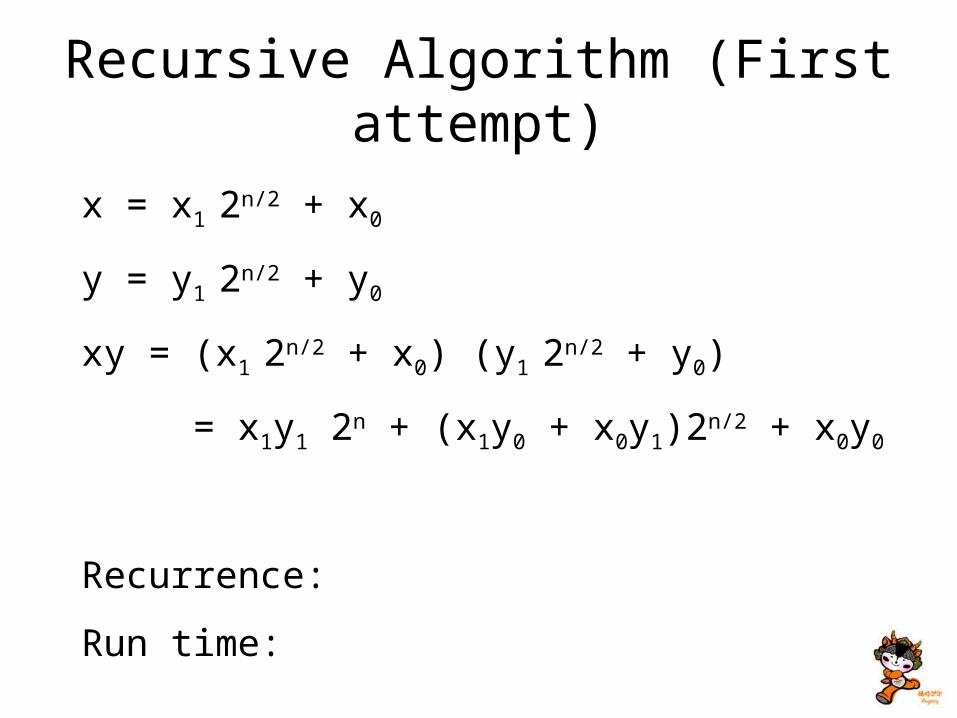
Recursive Algorithm (First attempt)

x = x1 2n/2 + x0

y = y1 2n/2 + y0

xy = (x1 2n/2 + x0) (y1 2n/2 + y0)

= x1y1 2n + (x1y0 + x0y1)2n/2 + x0y0

Recurrence:

Run time:

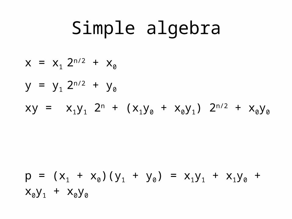
Simple algebra

x = x1 2n/2 + x0

y = y1 2n/2 + y0

xy = x1y1 2n + (x1y0 + x0y1) 2n/2 + x0y0

p = (x1 + x0)(y1 + y0) = x1y1 + x1y0 + x0y1 + x0y0

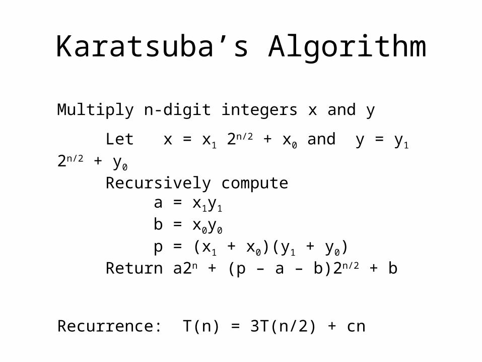
Karatsuba’s Algorithm

Multiply n-digit integers x and y

Let x = x1 2n/2 + x0 and y = y1 2n/2 + y0

Recursively computea = x1y1

b = x0y0

p = (x1 + x0)(y1 + y0) Return a2n + (p – a – b)2n/2 + b

Recurrence: T(n) = 3T(n/2) + cn

FFT, Convolution and Polynomial Multiplication

• Preview– FFT - O(n log n) algorithm

• Evaluate a polynomial of degree n at n points in O(n log n) time

– Computation of Convolution and Polynomial Multiplication (in O(n log n)) time

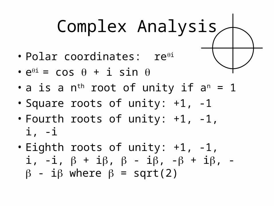
Complex Analysis

• Polar coordinates: rei

• ei = cos + i sin • a is a nth root of unity if an = 1

• Square roots of unity: +1, -1

• Fourth roots of unity: +1, -1, i, -i

• Eighth roots of unity: +1, -1, i, -i, + i, - i, - + i, - - i where = sqrt(2)

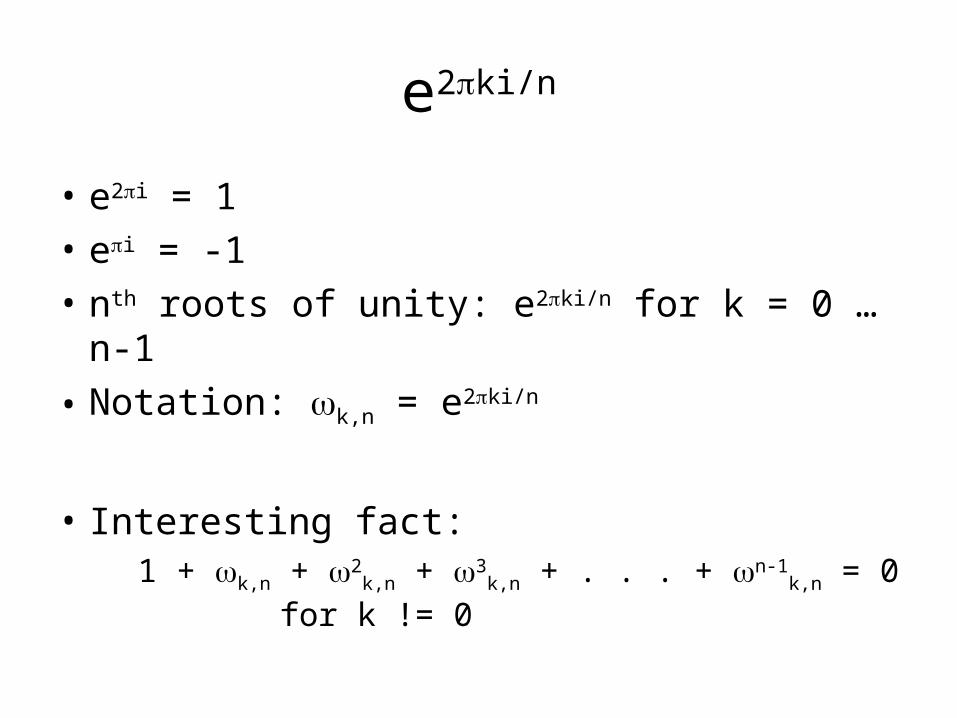
e2ki/n

• e2i = 1

• ei = -1

• nth roots of unity: e2ki/n for k = 0 …n-1

• Notation: k,n = e2ki/n

• Interesting fact: 1 + k,n + 2

k,n + 3k,n + . . . + n-1

k,n = 0 for k != 0

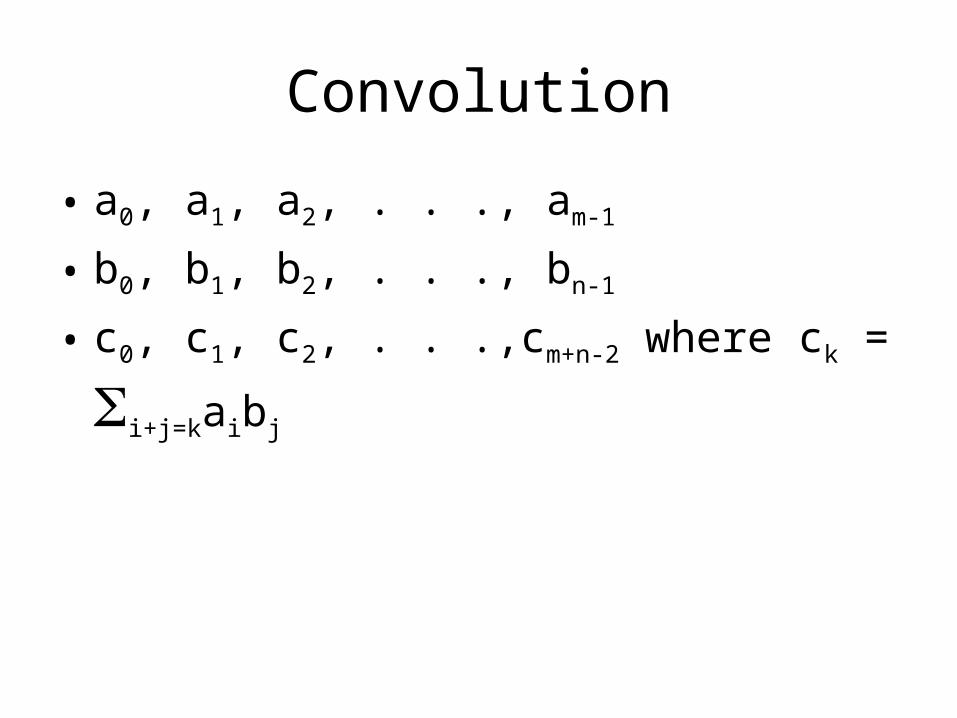
Convolution

• a0, a1, a2, . . ., am-1

• b0, b1, b2, . . ., bn-1

• c0, c1, c2, . . .,cm+n-2 where ck = i+j=kaibj

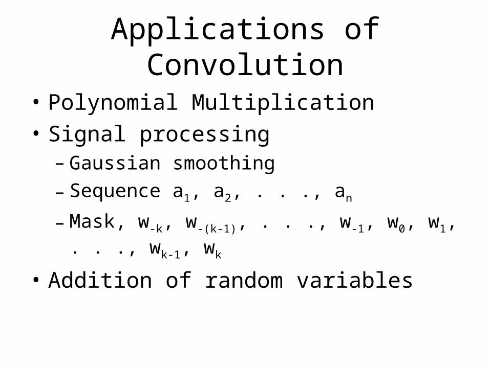
Applications of Convolution

• Polynomial Multiplication

• Signal processing– Gaussian smoothing

– Sequence a1, a2, . . ., an

– Mask, w-k, w-(k-1), . . ., w-1, w0, w1, . . ., wk-1, wk

• Addition of random variables

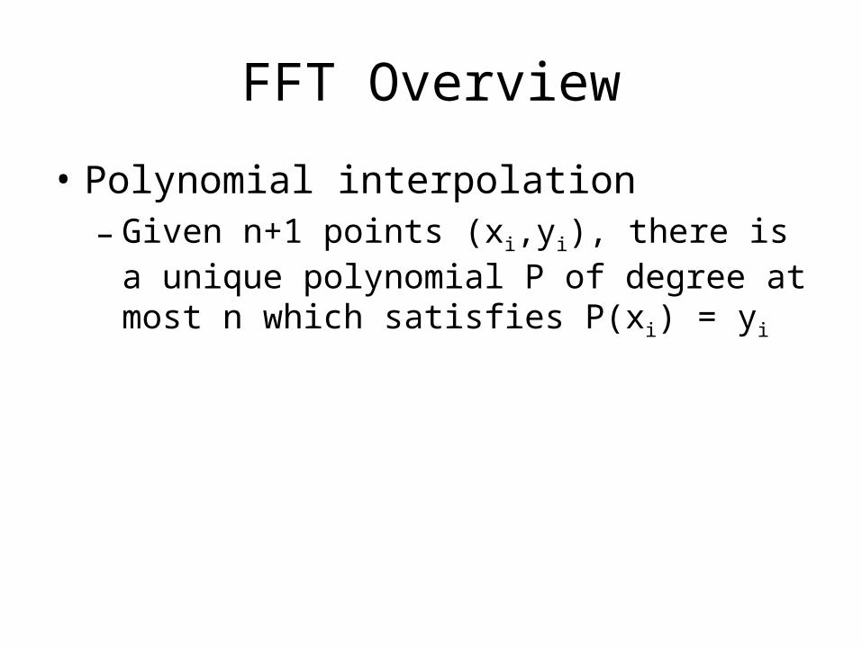
FFT Overview

• Polynomial interpolation– Given n+1 points (xi,yi), there is a unique

polynomial P of degree at most n which satisfies P(xi) = yi

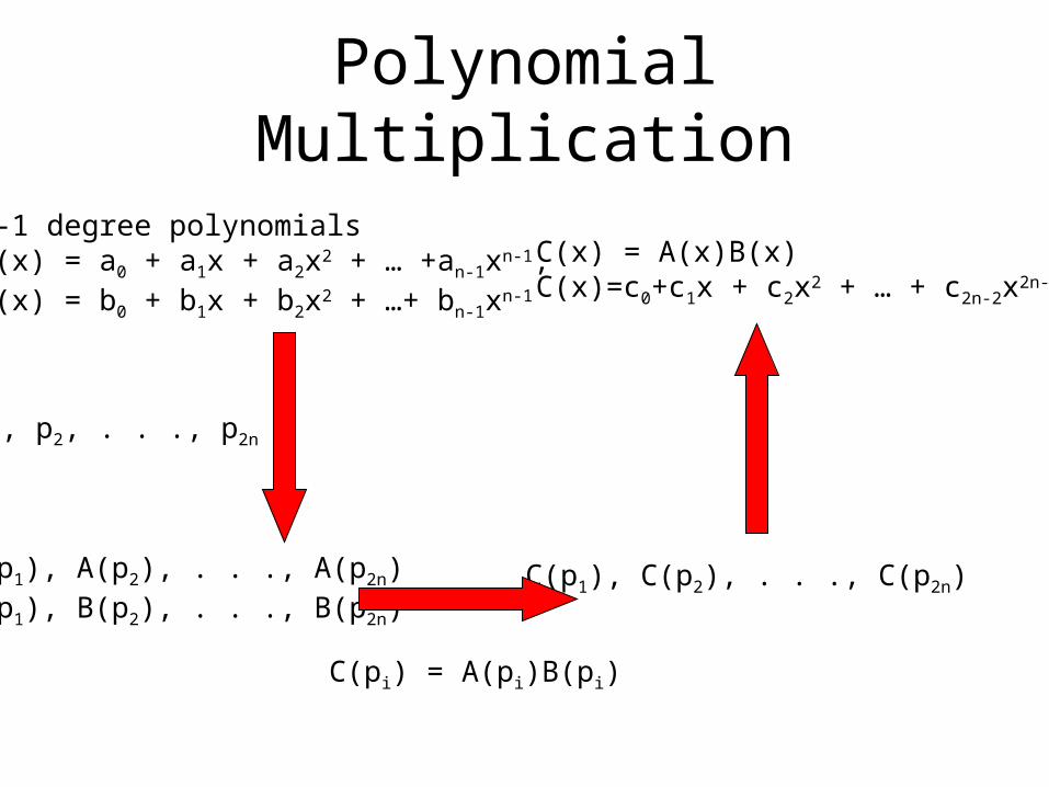
Polynomial Multiplication

n-1 degree polynomials A(x) = a0 + a1x + a2x2 + … +an-1xn-1,B(x) = b0 + b1x + b2x2 + …+ bn-1xn-1

C(x) = A(x)B(x)C(x)=c0+c1x + c2x2 + … + c2n-2x2n-2

p1, p2, . . ., p2n

A(p1), A(p2), . . ., A(p2n)B(p1), B(p2), . . ., B(p2n)

C(pi) = A(pi)B(pi)

C(p1), C(p2), . . ., C(p2n)

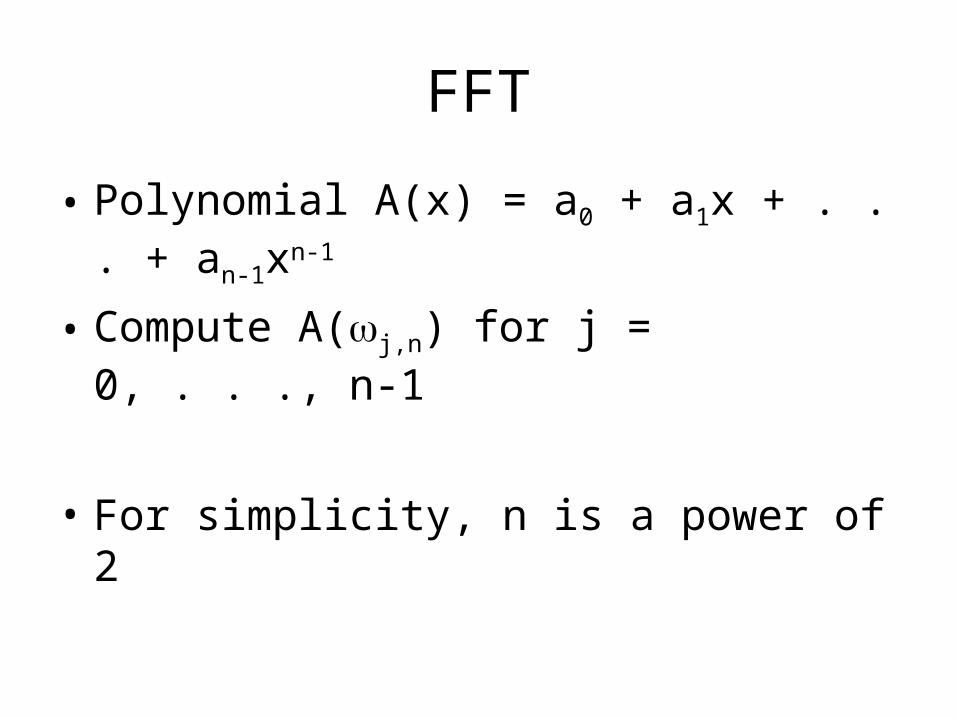
FFT

• Polynomial A(x) = a0 + a1x + . . . + an-1xn-1

• Compute A(j,n) for j = 0, . . ., n-1

• For simplicity, n is a power of 2

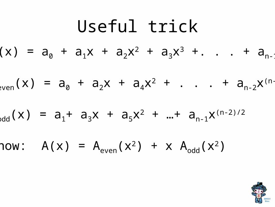
Useful trickA(x) = a0 + a1x + a2x2 + a3x3 +. . . + an-1xn-1

Aeven(x) = a0 + a2x + a4x2 + . . . + an-2x(n-2)/2

Aodd(x) = a1+ a3x + a5x2 + …+ an-1x(n-2)/2

Show: A(x) = Aeven(x2) + x Aodd(x2)

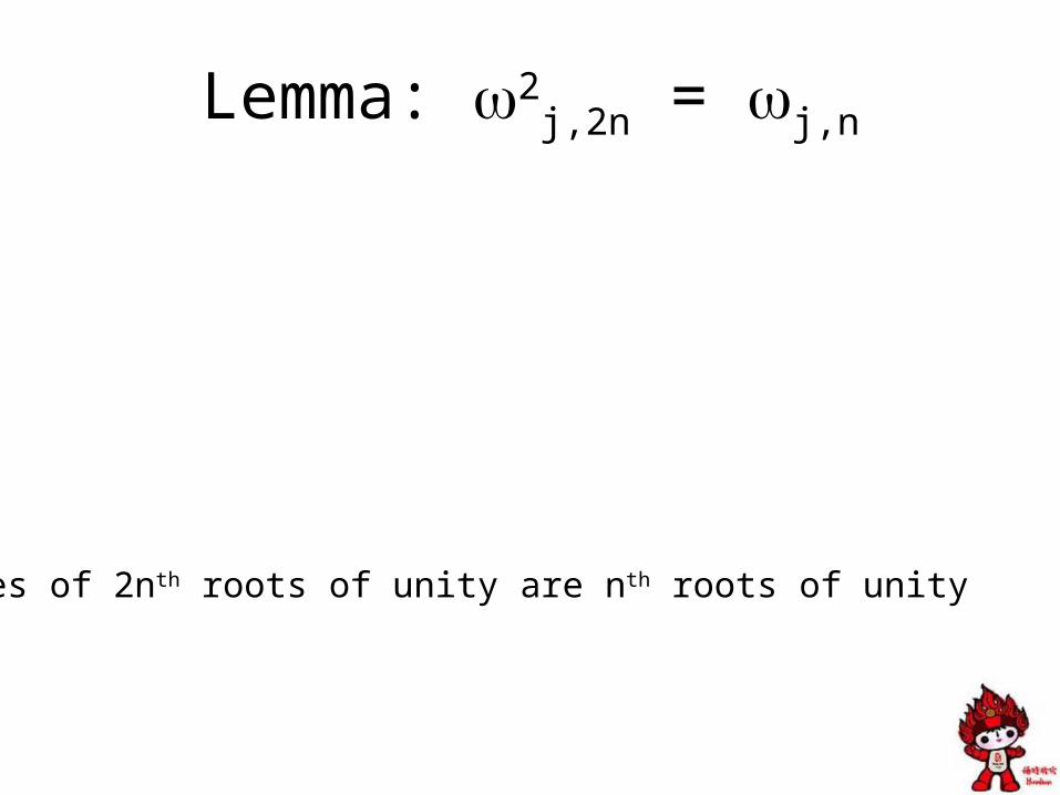
Lemma: 2j,2n = j,n

Squares of 2nth roots of unity are nth roots of unity

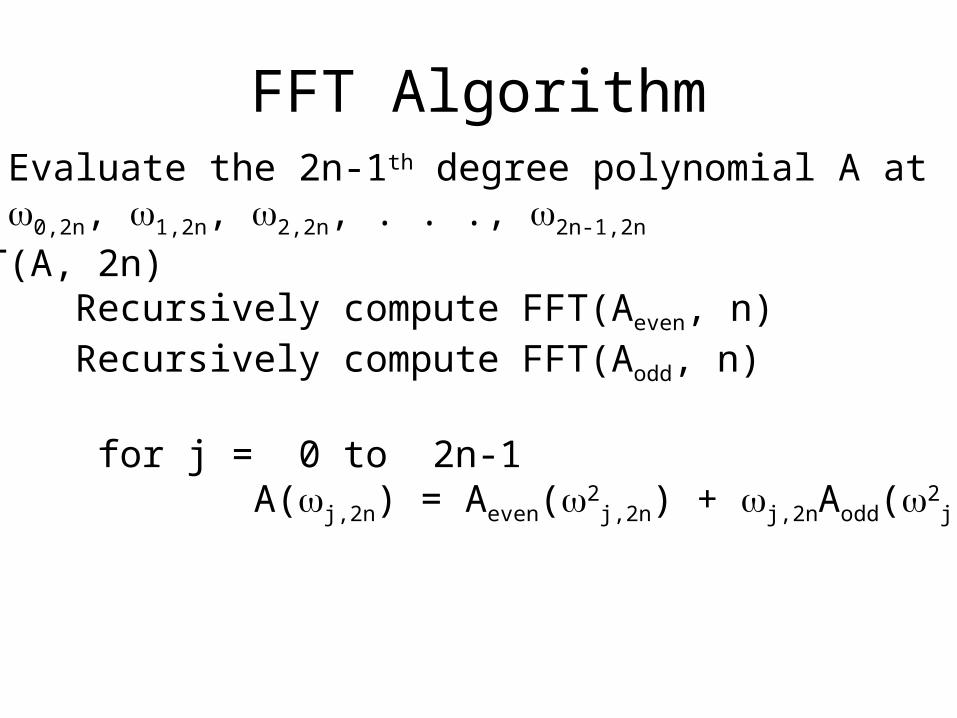
FFT Algorithm// Evaluate the 2n-1th degree polynomial A at// 0,2n, 1,2n, 2,2n, . . ., 2n-1,2n

FFT(A, 2n) Recursively compute FFT(Aeven, n) Recursively compute FFT(Aodd, n)

for j = 0 to 2n-1 A(j,2n) = Aeven(2

j,2n) + j,2nAodd(2j,2n)

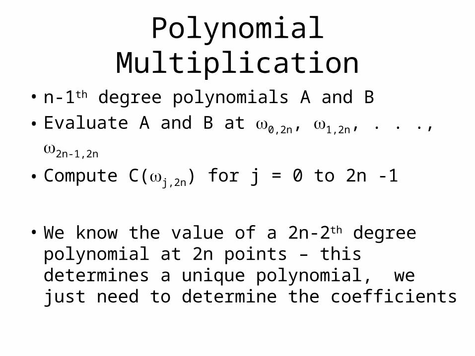
Polynomial Multiplication

• n-1th degree polynomials A and B

• Evaluate A and B at 0,2n, 1,2n, . . ., 2n-1,2n

• Compute C(j,2n) for j = 0 to 2n -1

• We know the value of a 2n-2th degree polynomial at 2n points – this determines a unique polynomial, we just need to determine the coefficients

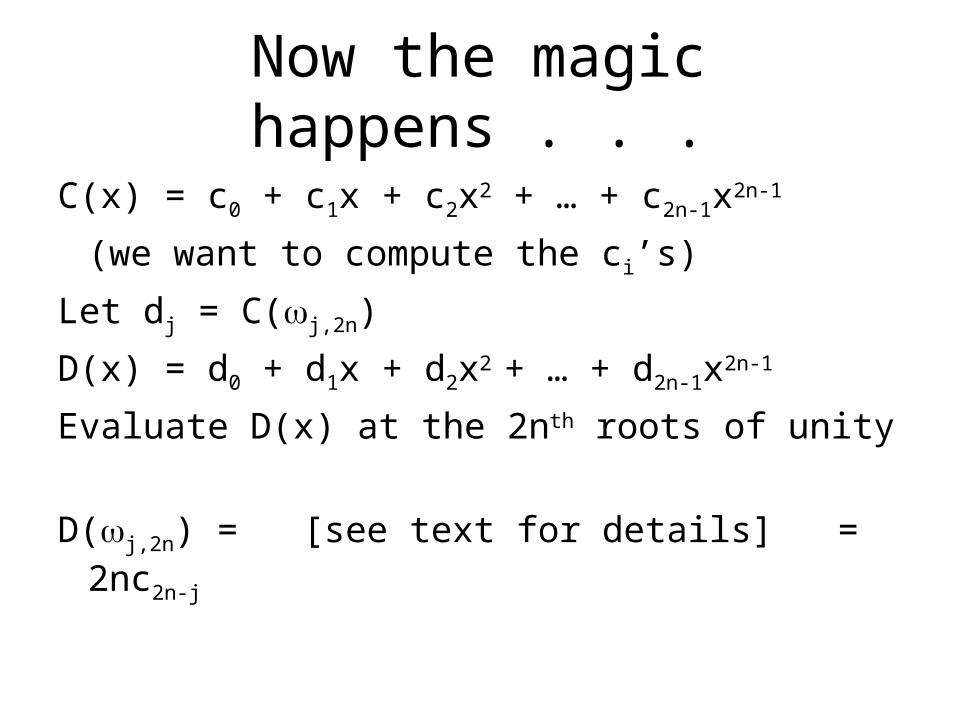
Now the magic happens . . .

C(x) = c0 + c1x + c2x2 + … + c2n-1x2n-1

(we want to compute the ci’s)

Let dj = C(j,2n)

D(x) = d0 + d1x + d2x2 + … + d2n-1x2n-1

Evaluate D(x) at the 2nth roots of unity

D(j,2n) = [see text for details] = 2nc2n-j

Polynomial Interpolation

• Build polynomial from the values of C at the 2nth roots of unity

• Evaluate this polynomial at the 2nth roots of unity