cse 3101: introduction to the design and analysis of ... · introduction to algorithms ( 3rd...
TRANSCRIPT

7/15/2010 CSE 3101 1
Instructor: Suprakash Datta ([email protected]) ext 77875
Lectures: Tues (BC 215), 7–10 PM
Office hours: Wed 4-6 pm (CSEB 3043), or by
appointment.
Textbook: Cormen, Leiserson, Rivest, Stein.Introduction to Algorithms (3rd Edition)
CSE 3101: Introduction to the Design and Analysis of Algorithms

7/15/2010 CSE 3101 2
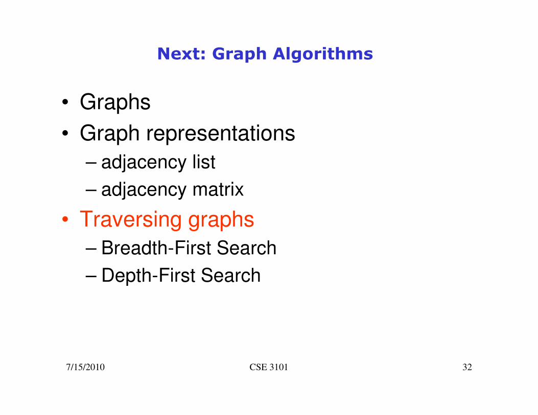
Next: Graph Algorithms
• Graphs
• Graph representations
– adjacency list
– adjacency matrix
• Traversing graphs
– Breadth-First Search
– Depth-First Search

7/15/2010 CSE 3101 3
Graphs – Definition
• A graph G = (V,E) is composed of:
– V: set of vertices
– E⊂ V× V: set of edges connecting the vertices
• An edge e = (u,v) is a pair of vertices
• (u,v) is ordered, if G is a directed graph

7/15/2010 CSE 3101 4
Graph Terminology
• adjacent vertices: connected by an edge
• degree (of a vertex): # of adjacent vertices
• path: sequence of vertices v1 ,v2 ,. . .vk such that consecutive vertices vi and vi+1 are adjacent
Since adjacent vertices each
count the adjoining edge, it will
be counted twice
deg( ) 2(# of edges)v V
v∈
=∑
7/15/2010 CSE 3101 5
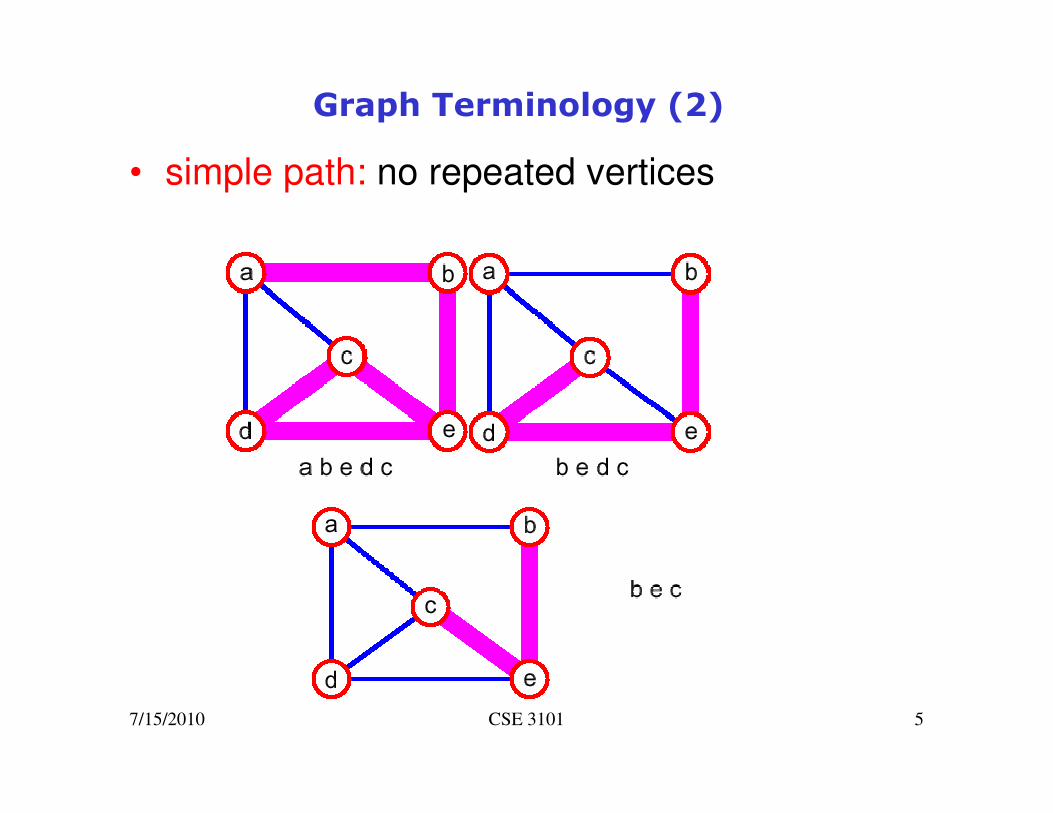
Graph Terminology (2)
• simple path: no repeated vertices
7/15/2010 CSE 3101 6
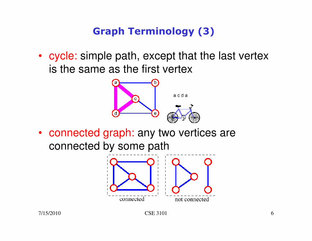
• cycle: simple path, except that the last vertex
is the same as the first vertex
• connected graph: any two vertices are
connected by some path
Graph Terminology (3)
7/15/2010 CSE 3101 7
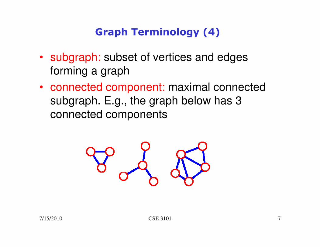
Graph Terminology (4)
• subgraph: subset of vertices and edges
forming a graph
• connected component: maximal connected
subgraph. E.g., the graph below has 3
connected components

7/15/2010 CSE 3101 8
Graph Terminology (5)
• (free) tree - connected graph without cycles
• forest - collection of trees
7/15/2010 CSE 3101 9
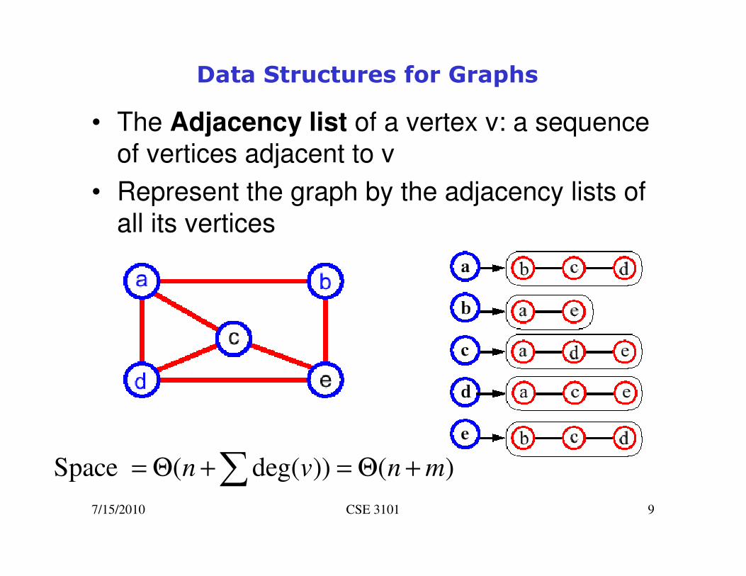
Data Structures for Graphs
• The Adjacency list of a vertex v: a sequence of vertices adjacent to v
• Represent the graph by the adjacency lists of
all its vertices
Space ( deg( )) ( )n v n m= Θ + = Θ +∑

7/15/2010 CSE 3101 10
• Adjacency matrix
• Matrix M with entries for all pairs of vertices
• M[i,j] = true – there is an edge (i,j) in the graph
• M[i,j] = false – there is no edge (i,j) in the graph
• Space = O(n2)
Data Structures for Graphs
7/15/2010 CSE 3101 11
Breadth First Search (2)
• In the second round, all the new edges that can be reached by unrolling the string 2 edges are visited and assigned a distance of 2
• This continues until every vertex has beenassigned a level
• The label of any vertex v corresponds to the length of the shortest path (in terms of edges) from s to v
7/15/2010 CSE 3101 12
Spanning Tree
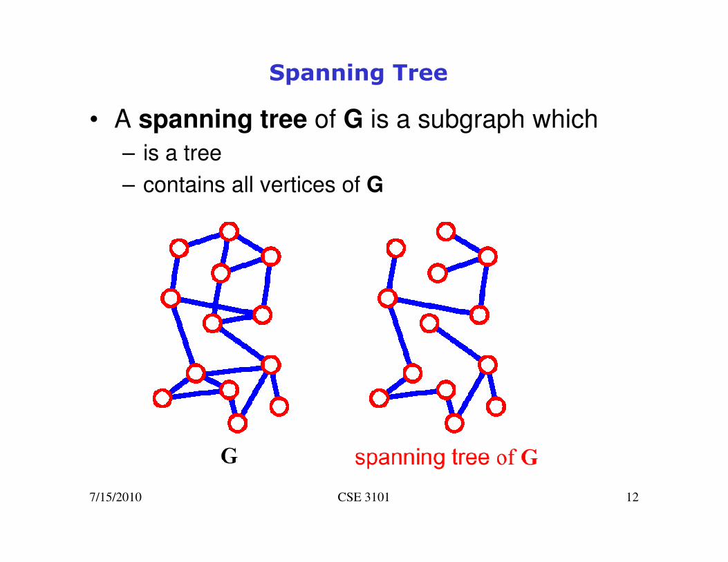
• A spanning tree of G is a subgraph which
– is a tree
– contains all vertices of G

7/15/2010 CSE 3101 13
Minimum Spanning Trees
• Undirected, connected
graph G = (V,E)
• Weight function W: E → R (assigning cost or length or
other values to edges)
( , )
( ) ( , )u v T
w T w u v∈
= ∑
� Spanning tree: tree that connects all vertices
� Minimum spanning tree: tree that connects all
the vertices and minimizes
7/15/2010 CSE 3101 14
Optimal Substructure
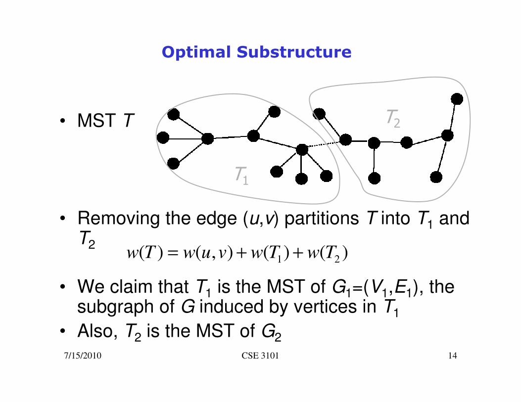
• MST T
• Removing the edge (u,v) partitions T into T1 and T2
• We claim that T1 is the MST of G1=(V1,E1), the subgraph of G induced by vertices in T1
• Also, T2 is the MST of G2
1 2( ) ( , ) ( ) ( )w T w u v w T w T= + +
T1
T2
7/15/2010 CSE 3101 15
Greedy Choice
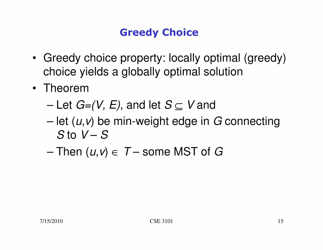
• Greedy choice property: locally optimal (greedy)
choice yields a globally optimal solution
• Theorem
– Let G=(V, E), and let S ⊆ V and
– let (u,v) be min-weight edge in G connecting
S to V – S
– Then (u,v) ∈ T – some MST of G
7/15/2010 CSE 3101 16
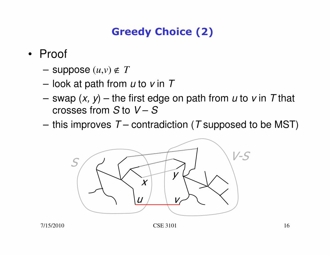
Greedy Choice (2)
• Proof
– suppose (u,v) ∉ T
– look at path from u to v in T
– swap (x, y) – the first edge on path from u to v in T that
crosses from S to V – S
– this improves T – contradiction (T supposed to be MST)
u v
xy
SV-S
7/15/2010 CSE 3101 17
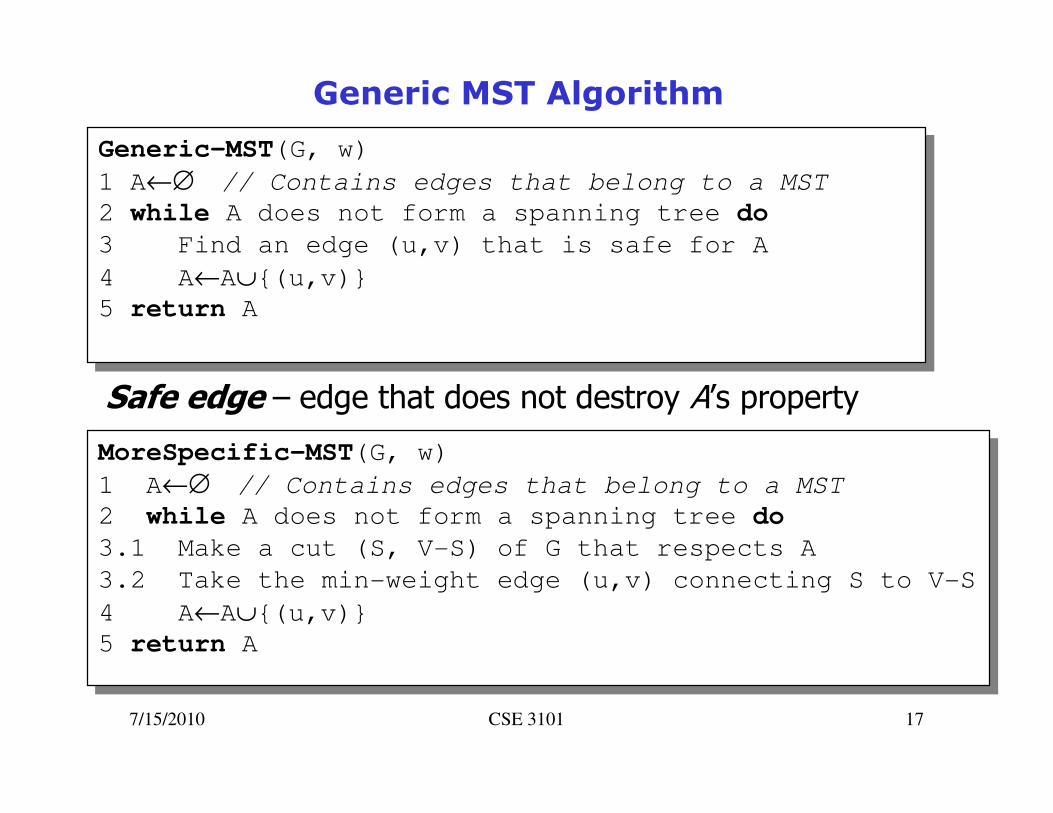
Generic MST Algorithm
Generic-MST(G, w)
1 A←∅ // Contains edges that belong to a MST
2 while A does not form a spanning tree do
3 Find an edge (u,v) that is safe for A
4 A←A∪{(u,v)}
5 return A
Generic-MST(G, w)
1 A←∅ // Contains edges that belong to a MST
2 while A does not form a spanning tree do
3 Find an edge (u,v) that is safe for A
4 A←A∪{(u,v)}
5 return A
Safe edge – edge that does not destroy A’s property
MoreSpecific-MST(G, w)
1 A←∅ // Contains edges that belong to a MST
2 while A does not form a spanning tree do
3.1 Make a cut (S, V-S) of G that respects A
3.2 Take the min-weight edge (u,v) connecting S to V-S
4 A←A∪{(u,v)}
5 return A
MoreSpecific-MST(G, w)
1 A←∅ // Contains edges that belong to a MST
2 while A does not form a spanning tree do
3.1 Make a cut (S, V-S) of G that respects A
3.2 Take the min-weight edge (u,v) connecting S to V-S
4 A←A∪{(u,v)}
5 return A

7/15/2010 CSE 3101 18
Prim’s Algorithm
• Vertex based algorithm
• Grows one tree T, one vertex at a time
• A cloud covering the portion of T already computed
• Label the vertices v outside the cloud with key[v] – the minimum weight of an edge connecting v to a vertex in the
cloud, key[v] = ∞, if no such edge exists
7/15/2010 CSE 3101 19
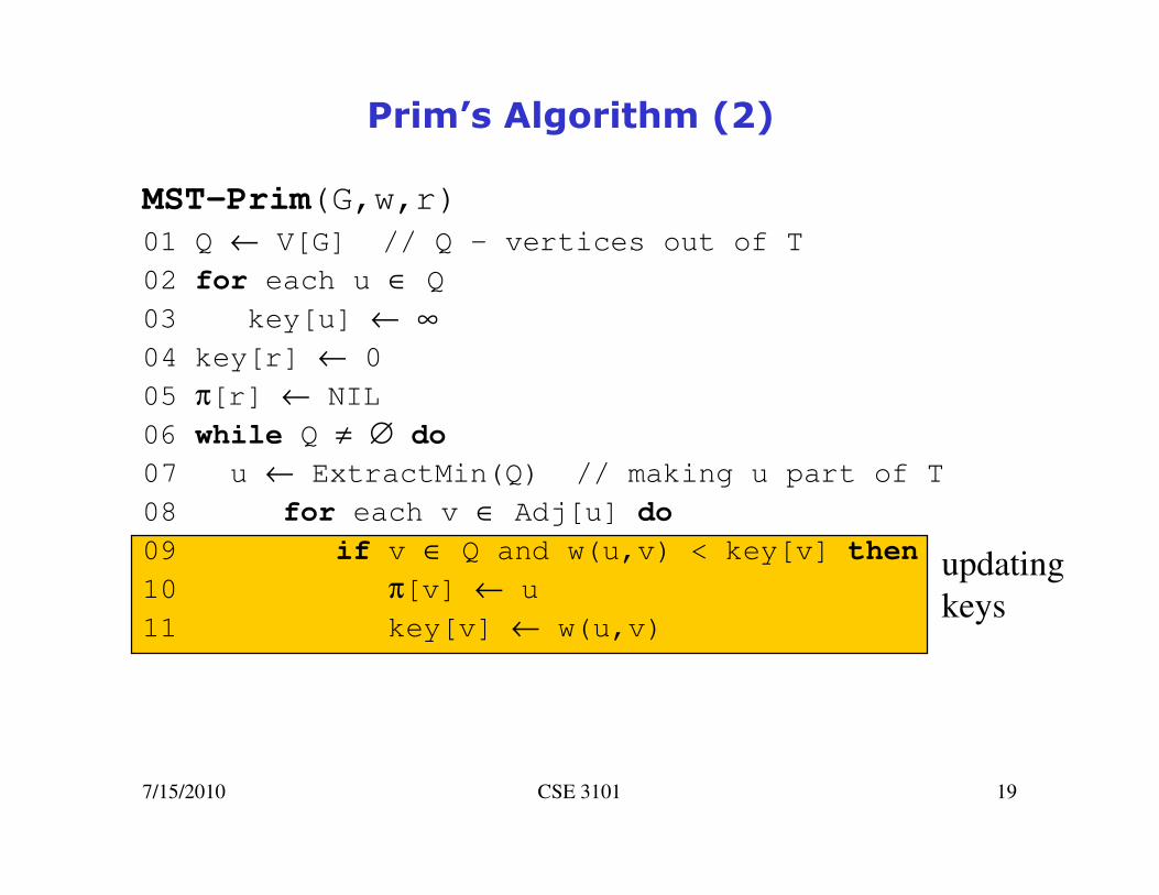
MST-Prim(G,w,r)
01 Q ← V[G] // Q – vertices out of T
02 for each u ∈ Q
03 key[u] ← ∞
04 key[r] ← 0
05 π[r] ← NIL
06 while Q ≠ ∅ do
07 u ← ExtractMin(Q) // making u part of T
08 for each v ∈ Adj[u] do
09 if v ∈ Q and w(u,v) < key[v] then
10 π[v] ← u
11 key[v] ← w(u,v)
Prim’s Algorithm (2)
updating
keys
7/15/2010 CSE 3101 20
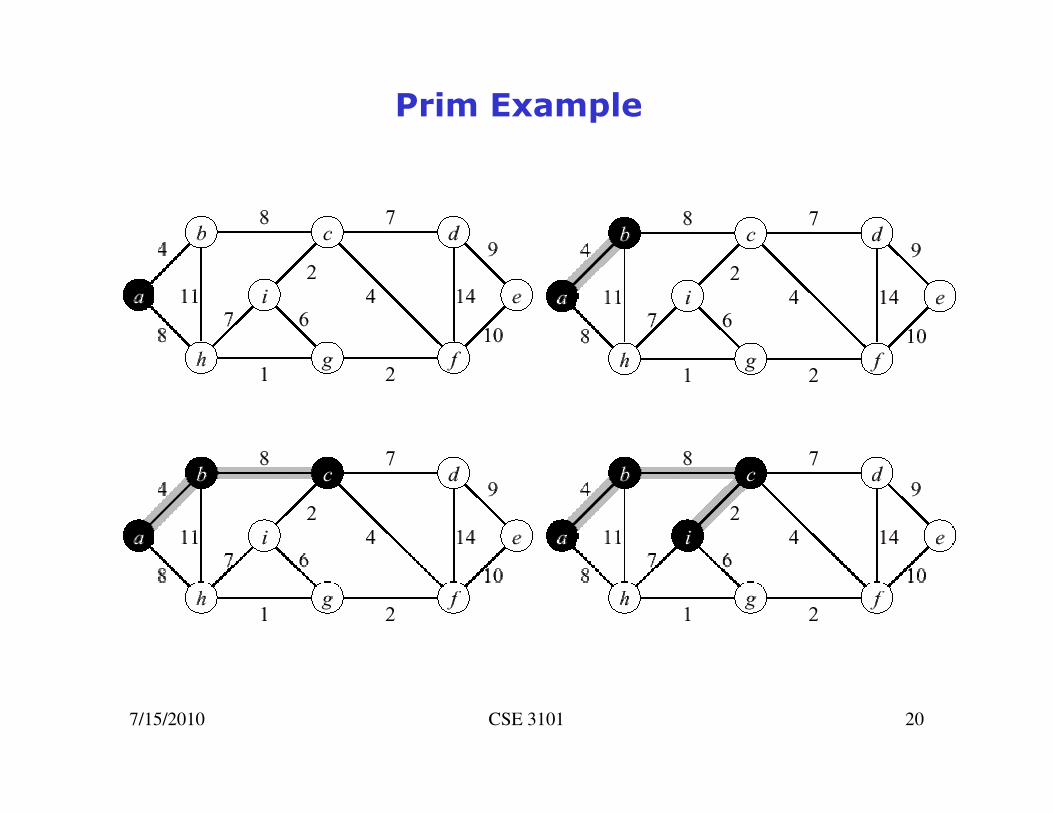
Prim Example

7/15/2010 CSE 3101 21
Prim Example (2)

7/15/2010 CSE 3101 22
Prim Example (3)

7/15/2010 CSE 3101 23
Priority Queues
• A priority queue is a data structure for
maintaining a set S of elements, each with an
associated value called key
• We need PQ to support the following operations
– BuildPQ(S) – initializes PQ to contain elements of S
– ExtractMin(S) returns and removes the element of S
with the smallest key
– ModifyKey(S,x,newkey) – changes the key of x in S
• A binary heap can be used to implement a PQ
– BuildPQ – O(n)
– ExtractMin and ModifyKey – O(lg n)
7/15/2010 CSE 3101 24
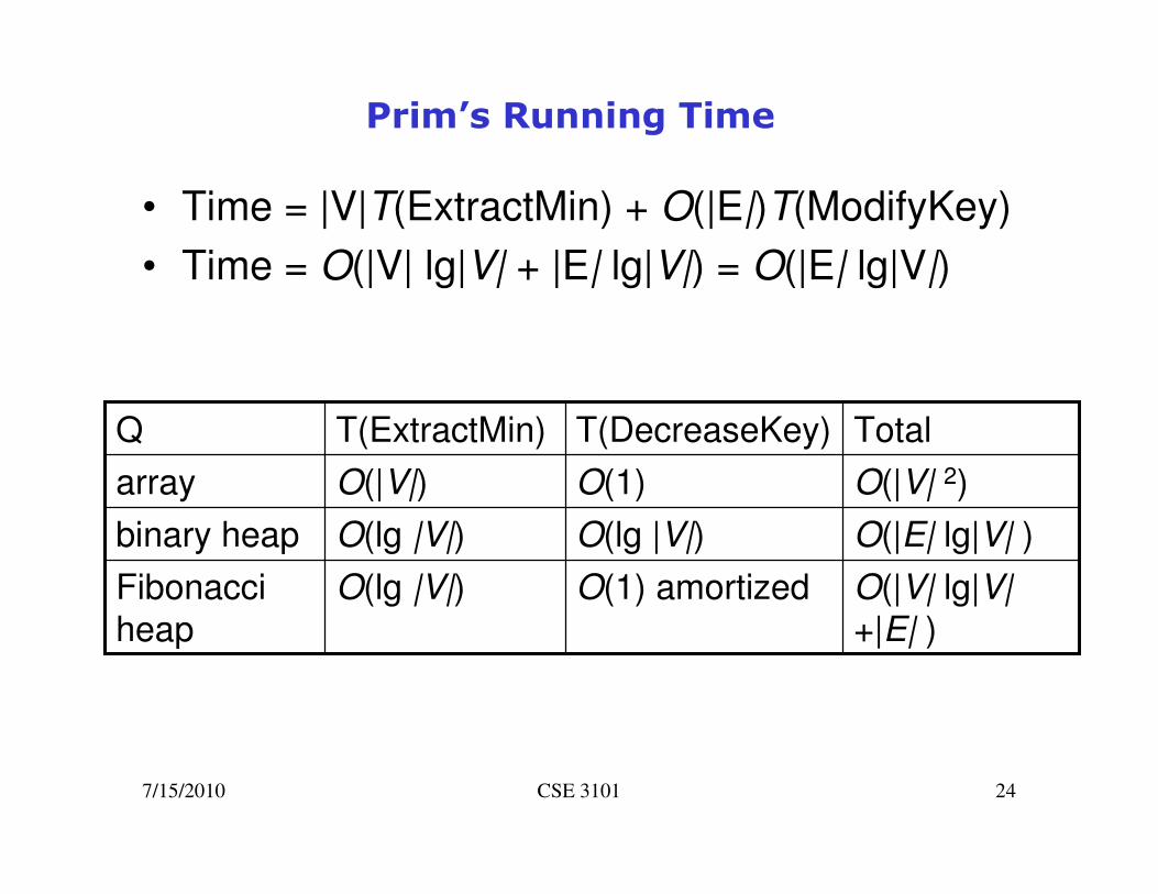
Prim’s Running Time
• Time = |V|T(ExtractMin) + O(|E|)T(ModifyKey)
• Time = O(|V| lg|V| + |E| lg|V|) = O(|E| lg|V|)
O(|V| lg|V|
+|E| )
O(1) amortizedO(lg |V|)Fibonacci
heap
O(|E| lg|V| )O(lg |V|)O(lg |V|)binary heap
O(|V| 2)O(1)O(|V|)array
TotalT(DecreaseKey)T(ExtractMin)Q

7/15/2010 CSE 3101 25
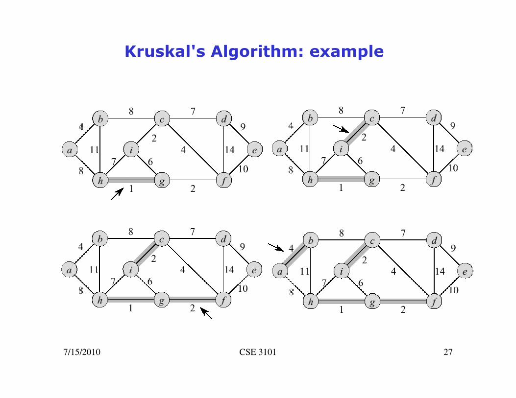
Kruskal's Algorithm
• Edge based algorithm
• Add the edges one at a time, in increasing weight order
• The algorithm maintains A – a forest of trees. An edge is accepted it if connects vertices of distinct trees
• We need an ADT that maintains a partition, i.e.,a collection of disjoint sets
– MakeSet(S,x): S ← S ∪ {{x}}
– Union(Si,Sj): S ← S – {Si,Sj} ∪ {Si ∪ Sj}
– FindSet(S, x): returns unique Si ∈ S, where x ∈
Si

7/15/2010 CSE 3101 26
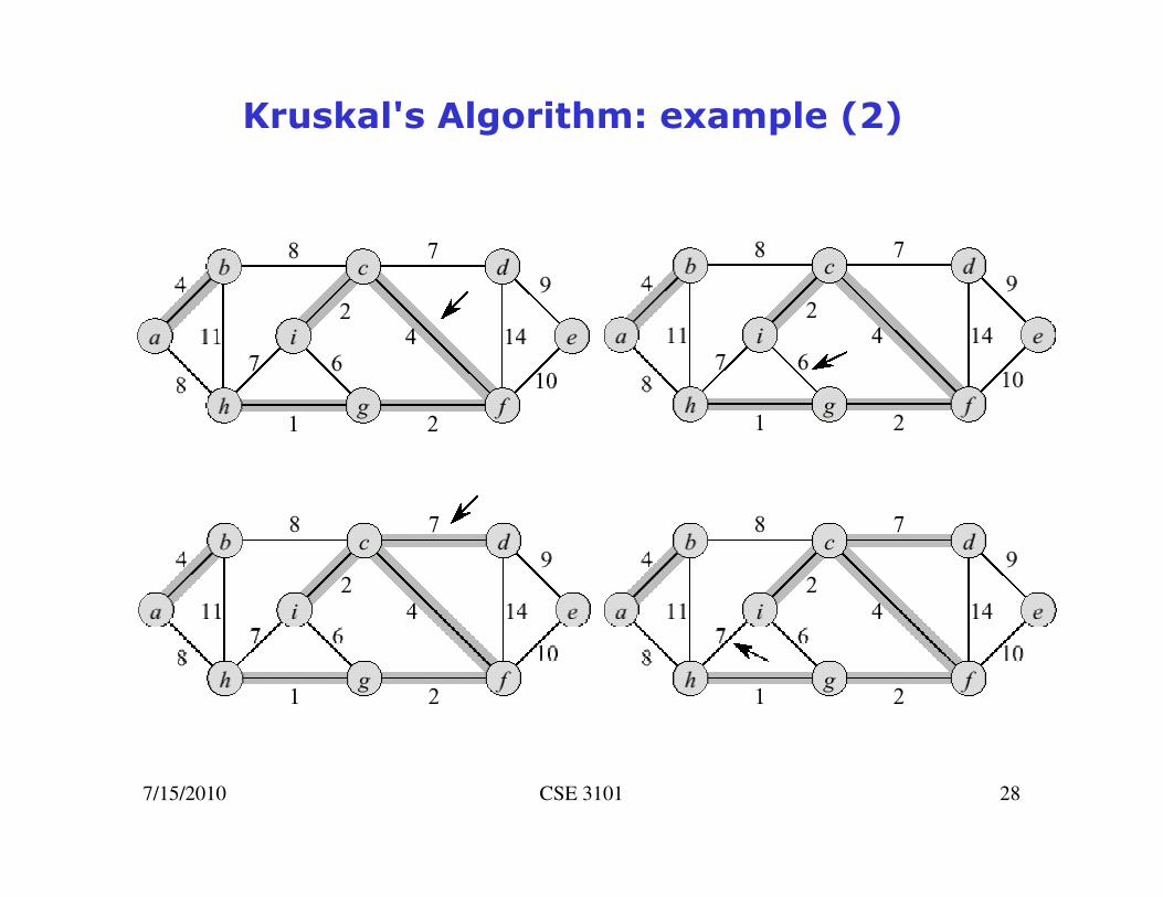
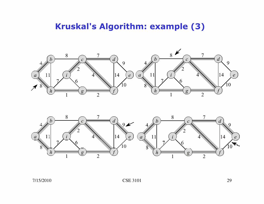
Kruskal's Algorithm
• The algorithm keeps adding the cheapest edge
that connects two trees of the forest
MST-Kruskal(G,w)
01 A ← ∅
02 for each vertex v ∈ V[G] do
03 Make-Set(v)
04 sort the edges of E by non-decreasing weight w
05 for each edge (u,v)∈ E, in order by non-
decreasing weight do
06 if Find-Set(u) ≠ Find-Set(v) then
07 A ← A ∪ {(u,v)}
08 Union(u,v)
09 return A
7/15/2010 CSE 3101 27
Kruskal's Algorithm: example
7/15/2010 CSE 3101 28
Kruskal's Algorithm: example (2)
7/15/2010 CSE 3101 29
Kruskal's Algorithm: example (3)

7/15/2010 CSE 3101 30
Kruskal's Algorithm: example (4)

7/15/2010 CSE 3101 31
Kruskal running time
• Initialization O(|V|) time
• Sorting the edges Θ(|E| lg |E|) = Θ(|E| lg |V|) (why?)
• O(|E|) calls to FindSet
• Union costs– Let t(v) – the number of times v is moved to a new
cluster
– Each time a vertex is moved to a new cluster the size of the cluster containing the vertex at least doubles: t(v) ≤ log |V|
– Total time spent doing Union
• Total time: O(|E| lg |V|) ( ) log
v V
t v V V∈
≤∑
7/15/2010 CSE 3101 32
Next: Graph Algorithms
• Graphs
• Graph representations
– adjacency list
– adjacency matrix
• Traversing graphs
– Breadth-First Search
– Depth-First Search
7/15/2010 CSE 3101 33
Graph Searching Algorithms
• Systematic search of every edge and vertex of the graph
• Graph G = (V,E) is either directed or undirected
• Today's algorithms assume an adjacency list representation
• Applications– Compilers
– Graphics
– Maze-solving
– Mapping
– Networks: routing, searching, clustering, etc.
7/15/2010 CSE 3101 34
Breadth First Search
• A Breadth-First Search (BFS) traverses aconnected component of a graph, and in doing so defines a spanning tree with several useful properties
• BFS in an undirected graph G is like wandering in a labyrinth with a string.
• The starting vertex s, it is assigned a distance 0.
• In the first round, the string is unrolled the lengthof one edge, and all of the edges that are only one edge away from the anchor are visited(discovered), and assigned distances of 1

7/15/2010 CSE 3101 35
Breadth First Search (2)
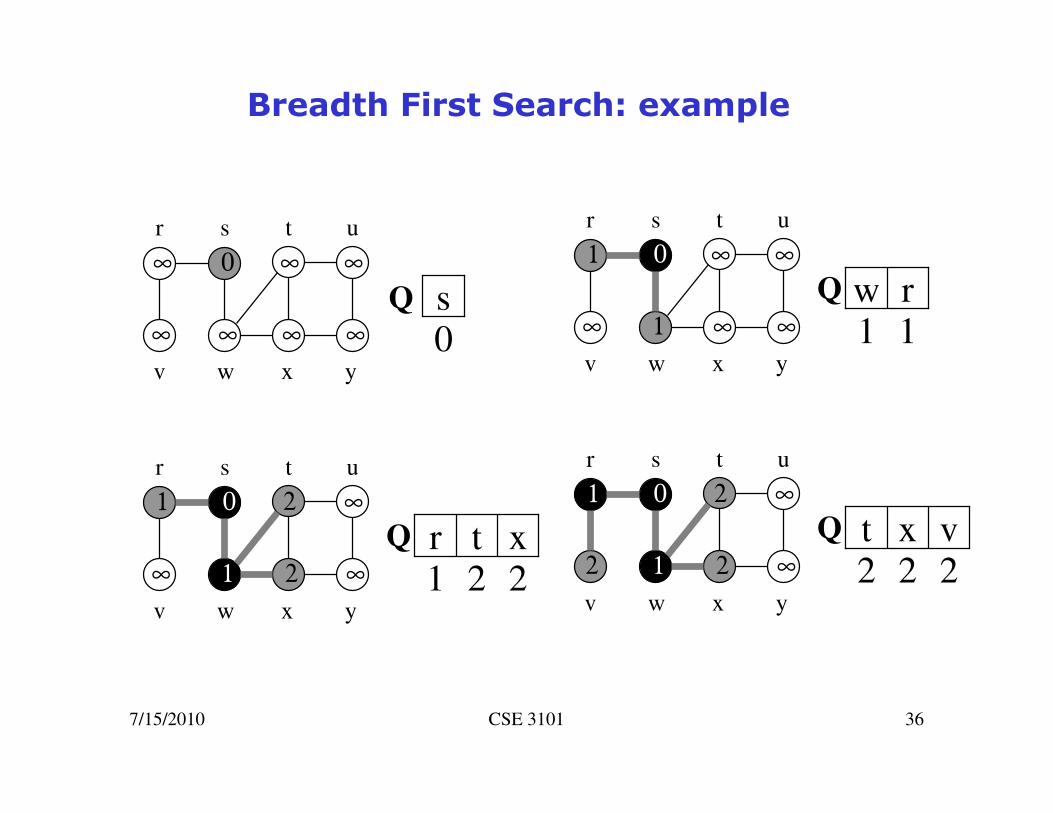
• In the second round, all the new edges that can be reached by unrolling the string 2 edges are visited and assigned a distance of 2
• This continues until every vertex has beenassigned a level
• The label of any vertex v corresponds to the length of the shortest path (in terms of edges) from s to v
7/15/2010 CSE 3101 36
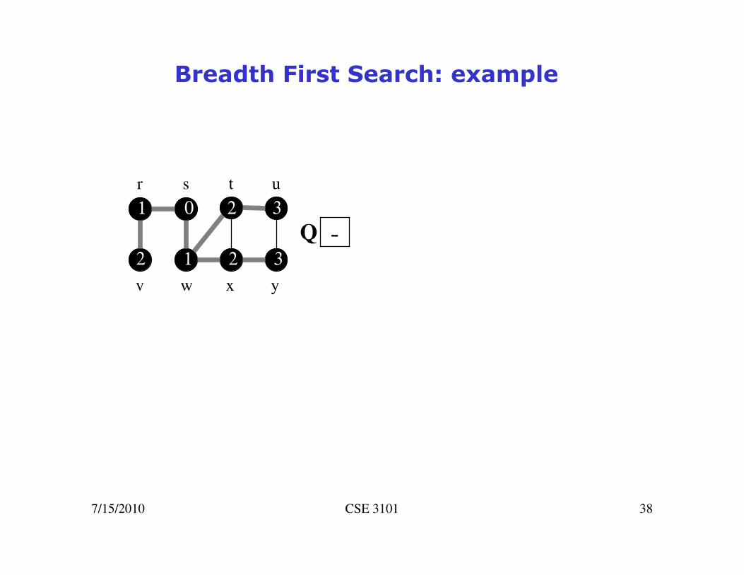
Breadth First Search: example
0∞
∞ ∞ ∞ ∞
r s u
∞
t
∞
wv yx
0sQ
01
∞ 1 ∞ ∞
r s u
∞
t
∞
wv yx
1w
1rQ
01
∞ 1 2 ∞
r s u
∞
t
2
wv yx
2t
1r
2xQ
01
2 1 2 ∞
r s u
∞
t
2
wv yx
2x
2t
2vQ

7/15/2010 CSE 3101 37
Breadth First Search: example
01
2 1 2 ∞
r s u
3
t
2
wv yx
2v
2x
3uQ
01
2 1 2 3
r s u
3
t
2
wv yx
3u
2v
3yQ
01
2 1 2 3
r s u
3
t
2
wv yx
3y
3uQ
01
2 1 2 3
r s u
3
t
2
wv yx
3yQ
7/15/2010 CSE 3101 38
Breadth First Search: example
01
2 1 2 3
r s u
3
t
2
wv yx
-Q
7/15/2010 CSE 3101 39
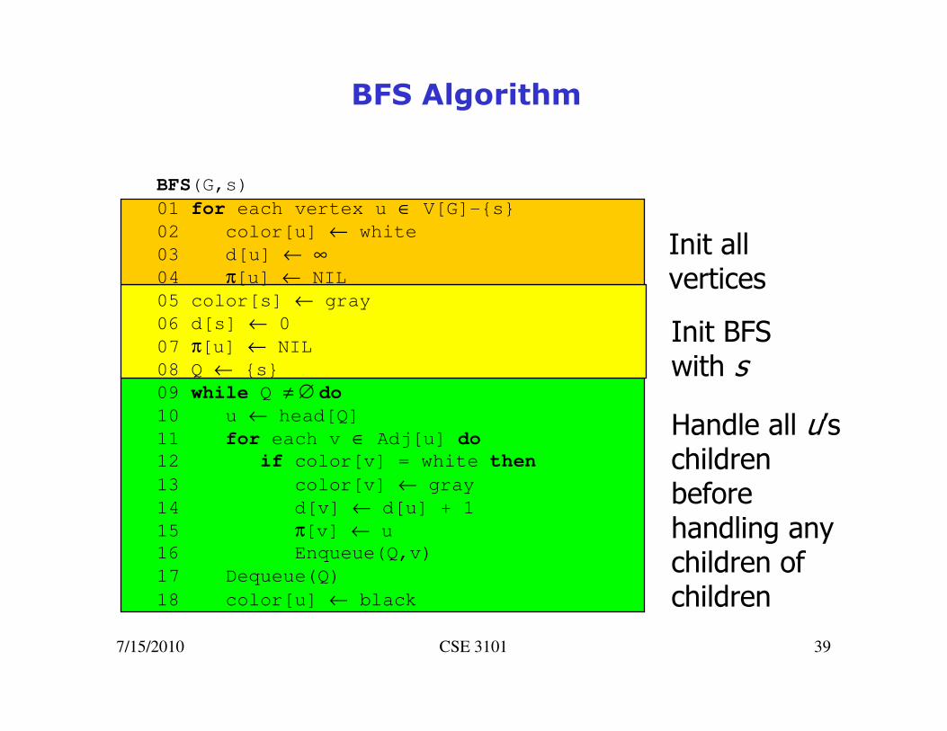
BFS Algorithm
BFS(G,s)
01 for each vertex u ∈ V[G]-{s}
02 color[u] ← white
03 d[u] ← ∞
04 π[u] ← NIL
05 color[s] ← gray
06 d[s] ← 0
07 π[u] ← NIL
08 Q ← {s}
09 while Q ≠ ∅ do
10 u ← head[Q]
11 for each v ∈ Adj[u] do
12 if color[v] = white then
13 color[v] ← gray
14 d[v] ← d[u] + 1
15 π[v] ← u
16 Enqueue(Q,v)
17 Dequeue(Q)
18 color[u] ← black
Init all vertices
Init BFS with s
Handle all u’s children before handling any children of children

7/15/2010 CSE 3101 40
BFS Algorithm: running time
• Given a graph G = (V,E)– Vertices are enqueued if there color is white
– Assuming that en- and dequeuing takes O(1) time the total cost of this operation is O(|V|)
– Adjacency list of a vertex is scanned when the vertex is dequeued (and only then…)
– The sum of the lengths of all lists is O(|E|). Consequently, O(|E|) time is spent on scanning them
– Initializing the algorithm takes O(|V|)
• Total running time O(|V|+|E|) (linear in the size of the adjacency list representation of G)

7/15/2010 CSE 3101 41
BFS Algorithm: properties
• Given a graph G = (V,E), BFS discovers all
vertices reachable from a source vertex s
• It computes the shortest distance to all reachable vertices
• It computes a breadth-first tree that contains all such reachable vertices
• For any vertex v reachable from s, the path in
the breadth first tree from s to v, corresponds
to a shortest path in G

7/15/2010 CSE 3101 42
BFS Tree
• Predecessor subgraph of G
• Gp is a breadth-first tree– Vp consists of the vertices reachable from s, and
– for all v ∈ Vp, there is a unique simple path from sto v in Gp that is also a shortest path from s to v in G
• The edges in Gp are called tree edges
{ } { }
{ }
( , )
: [ ]
( [ ], ) : { }
G V E
V v V v NIL s
E v v E v V s
π π π
π
π π
=
= ∈ π ≠ ∪
= π ∈ ∈ −
7/15/2010 CSE 3101 43
Depth-first search (DFS)
• A depth-first search (DFS) in an undirected graph G is like wandering in a labyrinth with a
string and a can of paint
– We start at vertex s, tying the end of our string to
the point and painting s “visited (discovered)”.
Next we label s as our current vertex called u
– Now, we travel along an arbitrary edge (u,v).
– If edge (u,v) leads us to an already visited vertex vwe return to u
– If vertex v is unvisited, we unroll our string, move to v, paint v “visited”, set v as our current vertex,
and repeat the previous steps

7/15/2010 CSE 3101 44
Depth-first search (2)
• Eventually, we will get to a point where all
incident edges on u lead to visited vertices
• We then backtrack by unrolling our string to a previously visited vertex v. Then v becomes our
current vertex and we repeat the previous steps
• Then, if all incident edges on v lead to visited
vertices, we backtrack as we did before. We
continue to backtrack along the path we
have traveled, finding and exploring unexplored edges, and repeating the procedure

7/15/2010 CSE 3101 45
Depth-first search algorithm
• Initialize – color all vertices white
• Visit each and every white vertex using DFS-Visit
• Each call to DFS-Visit(u) roots a new tree of the depth-first forest at vertex u
• A vertex is white if it is undiscovered
• A vertex is gray if it has been discovered but not all of its edges have been discovered
• A vertex is black after all of its adjacent vertices have been discovered (the adj. list was examined completely)

7/15/2010 CSE 3101 46
Init all vertices
Depth-first search algorithm (2)
Visit all children recursively
7/15/2010 CSE 3101 47
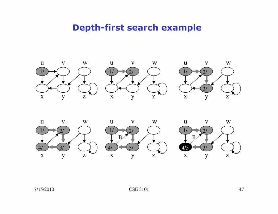
Depth-first search example
u
x
v w
y z
1/
u
x
v w
y z
1/ 2/
u
x
v w
y z
1/ 2/
3/
u
x
v w
y z
1/ 2/
3/4/
u
x
v w
y z
1/ 2/
3/4/
B
u
x
v w
y z
1/ 2/
3/4/5
B

7/15/2010 CSE 3101 48
Depth-first search example (2)
u
x
v w
y z
1/ 2/
3/64/5
B
u
x
v w
y z
1/ 2/7
3/64/5
B
u
x
v w
y z
1/ 2/7
3/64/5
BF
u
x
v w
y z
1/8 2/7
3/64/5
BF
u
x
v w
y z
1/8 2/7
3/64/5
BF
9/
u
x
v w
y z
1/8 2/7
3/64/5
BF
9/C

7/15/2010 CSE 3101 49
Depth-first search example (3)
u
x
v w
y z
1/8 2/7
3/64/5
BF
9/C
10/
u
x
v w
y z
1/8 2/7
3/64/5
BF
9/C
10/ B
u
x
v w
y z
1/8 2/7
3/64/5
BF
9/C
10/11 B
u
x
v w
y z
1/8 2/7
3/64/5
BF
9/12C
10/11 B
7/15/2010 CSE 3101 50
Depth-first search example (4)
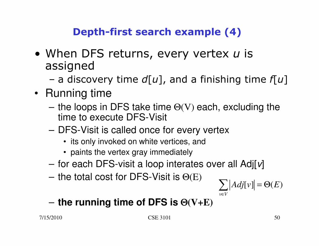
• When DFS returns, every vertex u is assigned– a discovery time d[u], and a finishing time f[u]
• Running time– the loops in DFS take time Θ(V) each, excluding the
time to execute DFS-Visit
– DFS-Visit is called once for every vertex• its only invoked on white vertices, and
• paints the vertex gray immediately
– for each DFS-visit a loop interates over all Adj[v]
– the total cost for DFS-Visit is Θ(E)
– the running time of DFS is ΘΘΘΘ(V+E)
[ ] ( )v V
Adj v E∈
= Θ∑
7/15/2010 CSE 3101 51
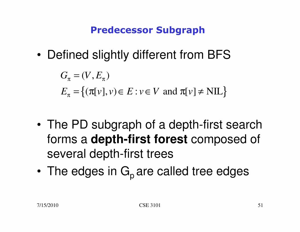
Predecessor Subgraph
• Defined slightly different from BFS
• The PD subgraph of a depth-first search forms a depth-first forest composed of several depth-first trees
• The edges in Gp are called tree edges
{ }
( , )
( [ ], ) : and [ ] NIL
G V E
E v v E v V v
π π
π
=
= π ∈ ∈ π ≠
7/15/2010 CSE 3101 52
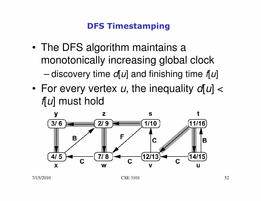
DFS Timestamping
• The DFS algorithm maintains a monotonically increasing global clock
– discovery time d[u] and finishing time f[u]
• For every vertex u, the inequality d[u] < f[u] must hold

7/15/2010 CSE 3101 53
DFS Timestamping
• Vertex u is
– white before time d[u]
– gray between time d[u] and time f[u], and
– black thereafter
• Notice the structure througout the algorithm.
– gray vertices form a linear chain
– correponds to a stack of vertices that have not been exhaustively explored (DFS-Visit started but not yet finished)

7/15/2010 CSE 3101 54
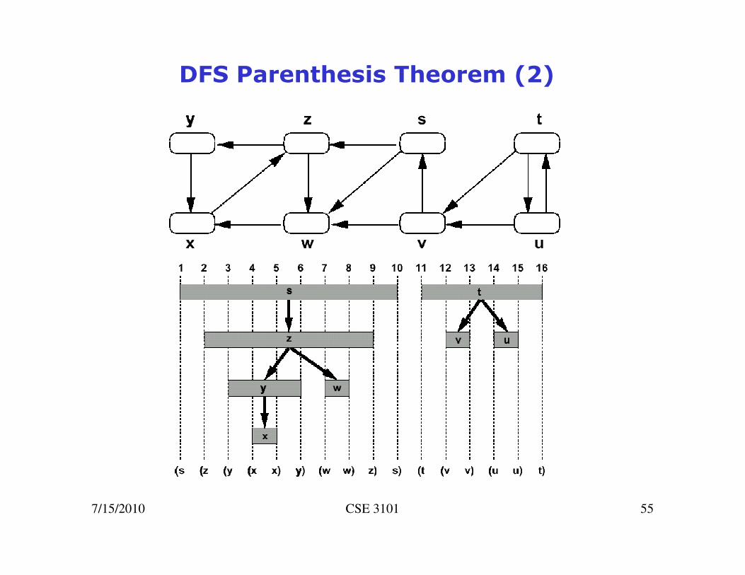
DFS Parenthesis Theorem
• Discovery and finish times have parenthesis structure– represent discovery of u with left parenthesis "(u"
– represent finishin of u with right parenthesis "u)"
– history of discoveries and finishings makes a well-formed expression (parenthesis are properly nested)
• Intuition for proof: any two intervals are either disjoint or enclosed– Overlaping intervals would mean finishing
ancestor, before finishing descendant or starting descendant without starting ancestor
7/15/2010 CSE 3101 55
DFS Parenthesis Theorem (2)

7/15/2010 CSE 3101 56
DFS Edge Classification
• Tree edge (gray to white)
– encounter new vertices (white)
• Back edge (gray to gray)
– from descendant to ancestor

7/15/2010 CSE 3101 57
DFS Edge Classification (2)
• Forward edge (gray to black)
– from ancestor to descendant
• Cross edge (gray to black)
– remainder – between trees or subtrees

7/15/2010 CSE 3101 58
DFS Edge Classification (3)
• Tree and back edges are important
• Most algorithms do not distinguish between
forward and cross edges
7/15/2010 CSE 3101 59
Next:
• Application of DFS: Topological Sort

7/15/2010 CSE 3101 60
Directed Acyclic Graphs
• A DAG is a directed graph with no cycles
• Often used to indicate precedences among events, i.e., event a must happen before b
• An example would be a parallel code execution
• Total order can be introduced using Topological Sorting
7/15/2010 CSE 3101 61
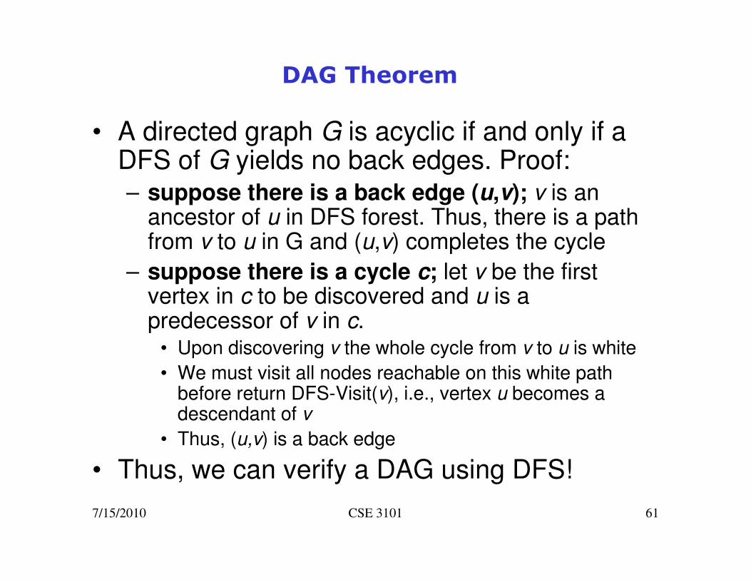
DAG Theorem
• A directed graph G is acyclic if and only if a DFS of G yields no back edges. Proof:– suppose there is a back edge (u,v); v is an
ancestor of u in DFS forest. Thus, there is a path from v to u in G and (u,v) completes the cycle
– suppose there is a cycle c; let v be the first vertex in c to be discovered and u is a predecessor of v in c.
• Upon discovering v the whole cycle from v to u is white
• We must visit all nodes reachable on this white path before return DFS-Visit(v), i.e., vertex u becomes a descendant of v
• Thus, (u,v) is a back edge
• Thus, we can verify a DAG using DFS!
7/15/2010 CSE 3101 62
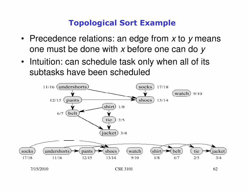
Topological Sort Example
• Precedence relations: an edge from x to y means
one must be done with x before one can do y
• Intuition: can schedule task only when all of its
subtasks have been scheduled
7/15/2010 CSE 3101 63
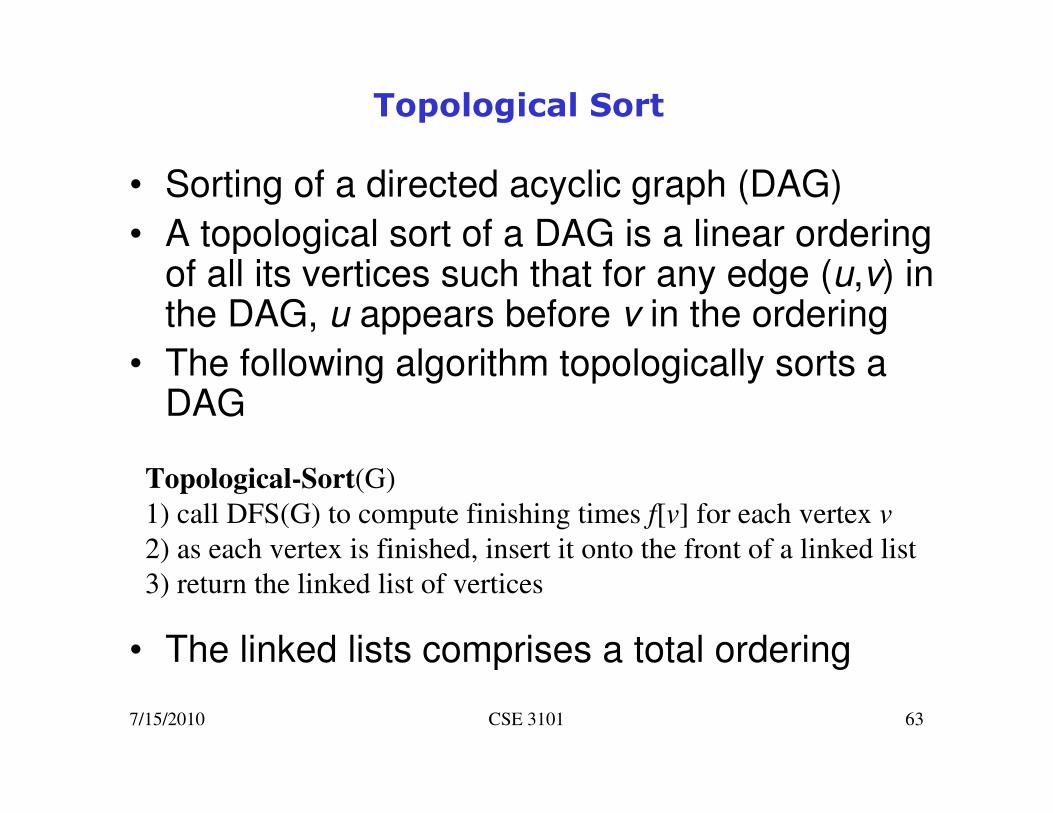
Topological Sort
• Sorting of a directed acyclic graph (DAG)
• A topological sort of a DAG is a linear ordering of all its vertices such that for any edge (u,v) in the DAG, u appears before v in the ordering
• The following algorithm topologically sorts a DAG
• The linked lists comprises a total ordering
Topological-Sort(G)
1) call DFS(G) to compute finishing times f[v] for each vertex v
2) as each vertex is finished, insert it onto the front of a linked list
3) return the linked list of vertices
7/15/2010 CSE 3101 64
Topological Sort
• Running time
– depth-first search: O(V+E) time
– insert each of the |V| vertices to the front of
the linked list: O(1) per insertion
• Thus the total running time is O(V+E)

7/15/2010 CSE 3101 65
Topological Sort Correctness
• Claim: for a DAG, an edge
• When (u,v) explored, u is gray. We can distinguish three cases– v = gray⇒ (u,v) = back edge (cycle, contradiction)
– v = white⇒ v becomes descendant of u⇒ v will be finished before u⇒ f[v] < f[u]
– v = black⇒ v is already finished⇒ f[v] < f[u]
• The definition of topological sort is satisfied
( , ) [ ] [ ]u v E f u f v∈ ⇒ >