cse 152, spring 2015 introduction to computer...

1

CSE 152, Spring 2015 Introduction to Computer Vision

Course Review

Introduction to Computer Vision

CSE 152

Lecture 20


Announcements

• Homework 3 has been graded and returned

• Homework 4 is due tomorrow, 11:59 PM– Will try to have graded and returned by

Monday, June 8

• Final exam is a take home exam


Course Review

• Human visual system

• Image formation and cameras

• Photometric image formation

• Color

• Binary image processing

• Filtering

• Edge detection and corner detection

• Hough transform and line fitting


Course Review

• Stereo

• Photometric stereo

• Recognition

• Motion

• Optical flow


Human Visual System


Structure of the eye

2


Rods and cones

Cones


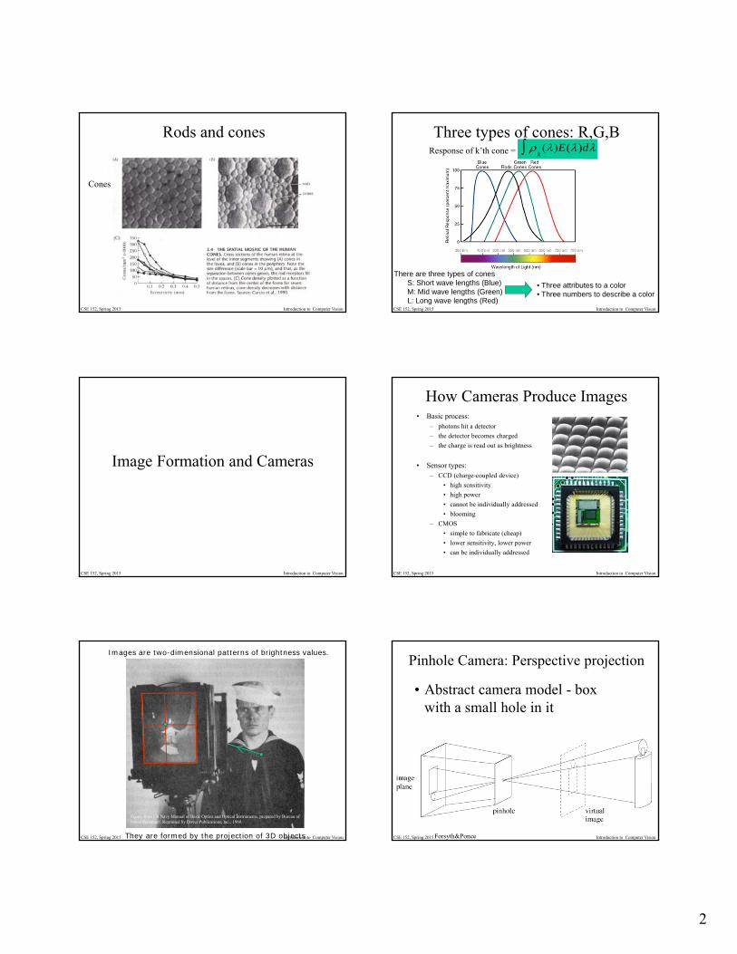
Three types of cones: R,G,B

There are three types of conesS: Short wave lengths (Blue)M: Mid wave lengths (Green)L: Long wave lengths (Red)

• Three attributes to a color• Three numbers to describe a color

Response of k’th cone = k()E()d


Image Formation and Cameras


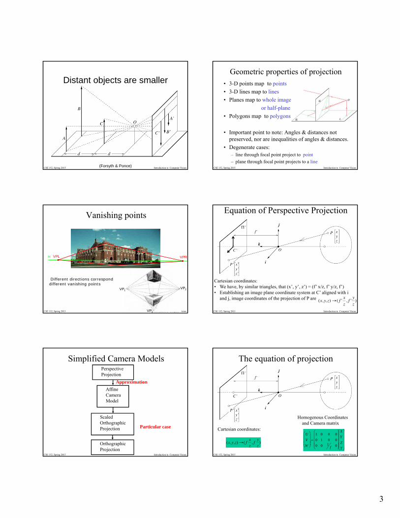
How Cameras Produce Images• Basic process:

– photons hit a detector

– the detector becomes charged

– the charge is read out as brightness

• Sensor types:– CCD (charge-coupled device)

• high sensitivity

• high power

• cannot be individually addressed

• blooming

– CMOS

• simple to fabricate (cheap)

• lower sensitivity, lower power

• can be individually addressed


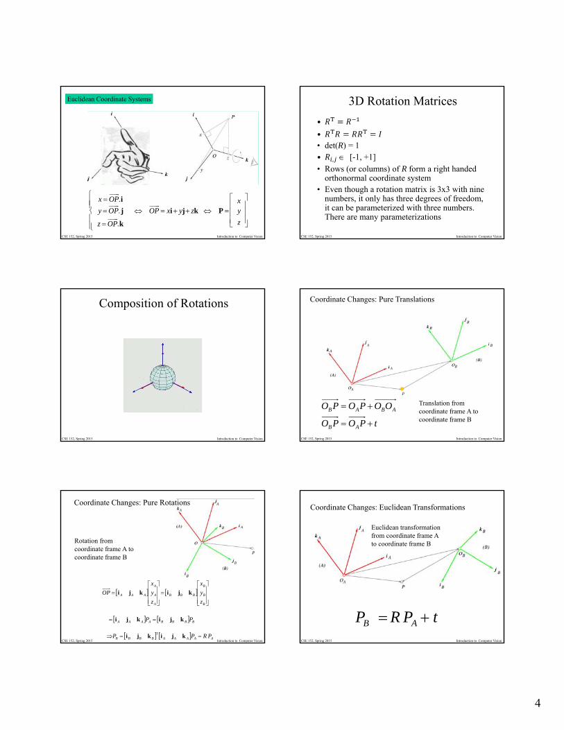
Images are two-dimensional patterns of brightness values.

They are formed by the projection of 3D objects.

Figure from US Navy Manual of Basic Optics and Optical Instruments, prepared by Bureau of Naval Personnel. Reprinted by Dover Publications, Inc., 1969.


Pinhole Camera: Perspective projection

• Abstract camera model - box with a small hole in it

Forsyth&Ponce

3


Distant objects are smaller

(Forsyth & Ponce) CSE 152, Spring 2015 Introduction to Computer Vision

Geometric properties of projection• 3-D points map to points

• 3-D lines map to lines

• Planes map to whole image

or half-plane

• Polygons map to polygons

• Important point to note: Angles & distances not preserved, nor are inequalities of angles & distances.

• Degenerate cases:– line through focal point project to point

– plane through focal point projects to a line


Vanishing points

VPL VPRH

VP1VP2

VP3

Different directions correspond different vanishing points


Equation of Perspective Projection

Cartesian coordinates:• We have, by similar triangles, that (x’, y’, z’) = (f’ x/z, f’ y/z, f’)• Establishing an image plane coordinate system at C’ aligned with i

and j, image coordinates of the projection of P are


Simplified Camera ModelsPerspectiveProjection

ScaledOrthographicProjection

AffineCameraModel

OrthographicProjection

Approximation

Particular case


The equation of projection

Cartesian coordinates:U

V

W

1 0 0 0

0 1 0 0

0 0 1f 0

X

Y

Z

T

Homogenous Coordinates and Camera matrix

4


Euclidean Coordinate Systems

x OP

.i

y OP

. j

z OP

.k

OP

xi yj zk P xy

z


3D Rotation Matrices

••• det(R) = 1• , [-1, +1]

• Rows (or columns) of R form a right handed orthonormal coordinate system

• Even though a rotation matrix is 3x3 with nine numbers, it only has three degrees of freedom, it can be parameterized with three numbers. There are many parameterizations


Composition of Rotations


Coordinate Changes: Pure Translations

tPOPO

OOPOPO

AB

ABAB

Translation from coordinate frame A to coordinate frame B


Coordinate Changes: Pure Rotations

B

B

B

BBB

A

A

A

AAA

z

y

x

z

y

x

OP kjikji

BBBBAAAA PP kjikji

AAAAAT

BBBB PRPP kjikji

Rotation from coordinate frame A to coordinate frame B


Coordinate Changes: Euclidean Transformations

tPRP AB

Euclidean transformation from coordinate frame A to coordinate frame B

5


Euclidean Transformations, Homogeneous Coordinates

11111

AAT

AB PE

PtRtPRP

0

Euclidean transformation represented by 4x4 Matrix

1T

tRE

0


What if camera coordinate system differs from object coordinate system

{c}

P{W}

1, Tcw

tRE

0

10100

0010

0001

Z

Y

X

fW

V

U

Camera coordinate frame

World coordinate frame


Intrinsic parameters

u

v

3x3 homogenous matrixFocal length:Principal Point: C’Units (e.g. pixels)Orientation and position of image coordinate systemPixel Aspect ratio


Camera parameters

• Extrinsic Parameters: Since camera may not be at the origin, there is a rigid transformation between the world coordinates and the camera coordinates

• Intrinsic parameters: Since scene units (e.g., cm) differ image units (e.g., pixels) and coordinate system may not be centered in image, we capture that with a 3x3 transformation comprised of focal length, principal point, pixel aspect ratio, angle between axes, etc.

T

Z

Y

X

W

V

U

parameters extrinsic

by drepresente

tiontransformaEuclidean

0100

0010

0001

parameters intrinsic

by drepresente

tionTransforma

3 x 3 4 x 4


Beyond the pinhole CameraGetting more light – Bigger Aperture


Thin Lens

O

• Rotationally symmetric about optical axis.• Spherical interfaces.

Optical axis

6


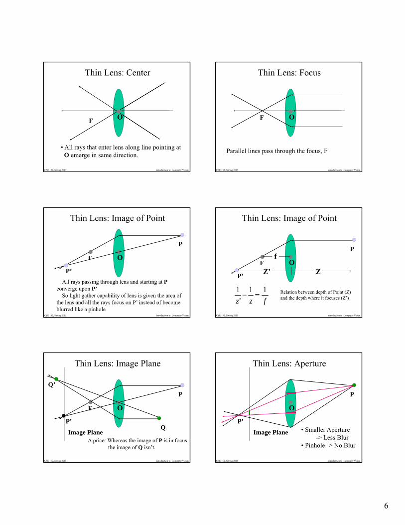
Thin Lens: Center

O

• All rays that enter lens along line pointing at O emerge in same direction.

F


Thin Lens: Focus

O

Parallel lines pass through the focus, F

F


Thin Lens: Image of Point

O

All rays passing through lens and starting at Pconverge upon P’

So light gather capability of lens is given the area of the lens and all the rays focus on P’ instead of become blurred like a pinhole

F

P

P’


Thin Lens: Image of Point

OF

P

P’Z’

f

Z

fzz

11

'

1 Relation between depth of Point (Z)

and the depth where it focuses (Z’)


Thin Lens: Image Plane

OF

P

P’

Image Plane

Q’

Q

A price: Whereas the image of P is in focus,the image of Q isn’t.


Thin Lens: Aperture

O

P

P’

Image Plane • Smaller Aperture-> Less Blur

• Pinhole -> No Blur

7


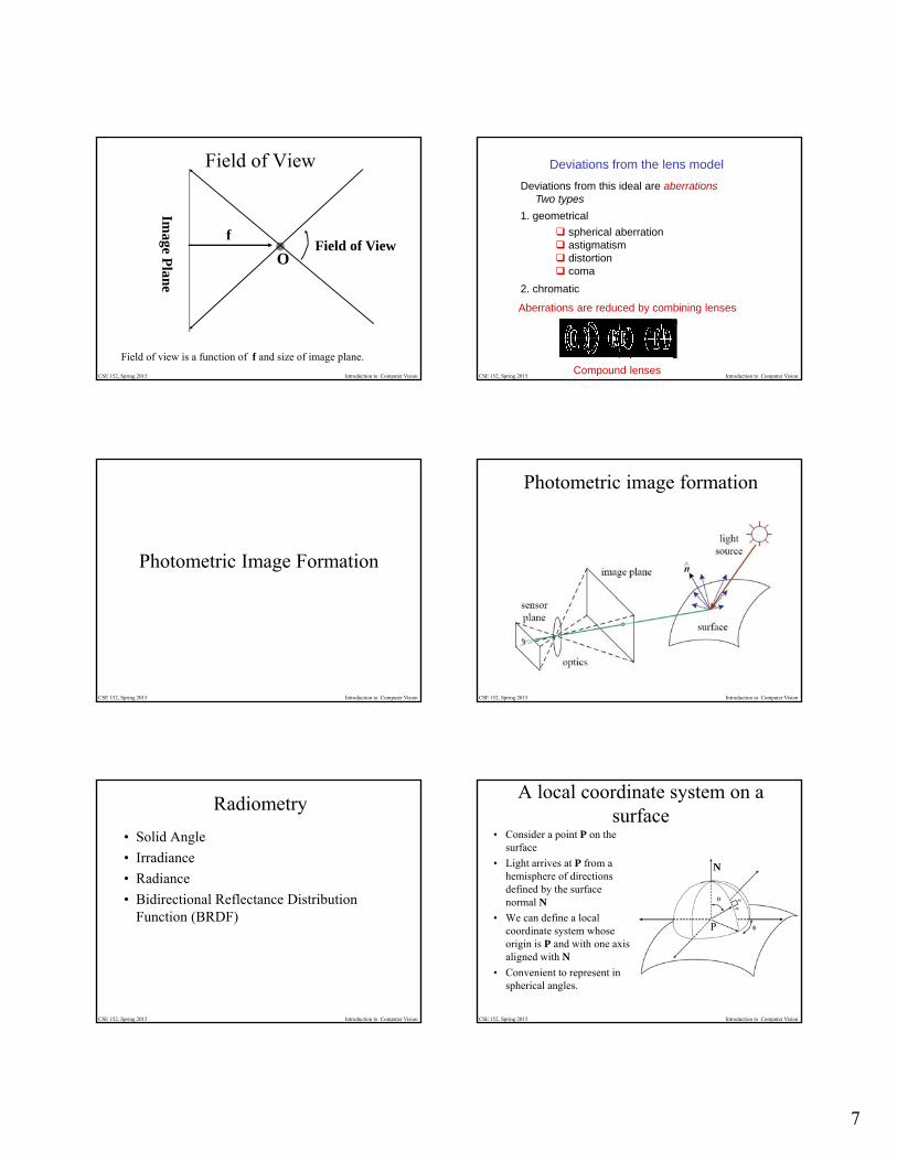
Field of View

OField of View

Image P

lane

f

Field of view is a function of f and size of image plane.


Deviations from this ideal are aberrationsTwo types

2. chromatic

1. geometrical

spherical aberration astigmatism distortion coma

Aberrations are reduced by combining lenses

Compound lenses

Deviations from the lens model


Photometric Image Formation


Photometric image formation


Radiometry

• Solid Angle

• Irradiance

• Radiance

• Bidirectional Reflectance Distribution Function (BRDF)


A local coordinate system on a surface

• Consider a point P on the surface

• Light arrives at P from a hemisphere of directions defined by the surface normal N

• We can define a local coordinate system whose origin is P and with one axis aligned with N

• Convenient to represent in spherical angles.

P

N

8


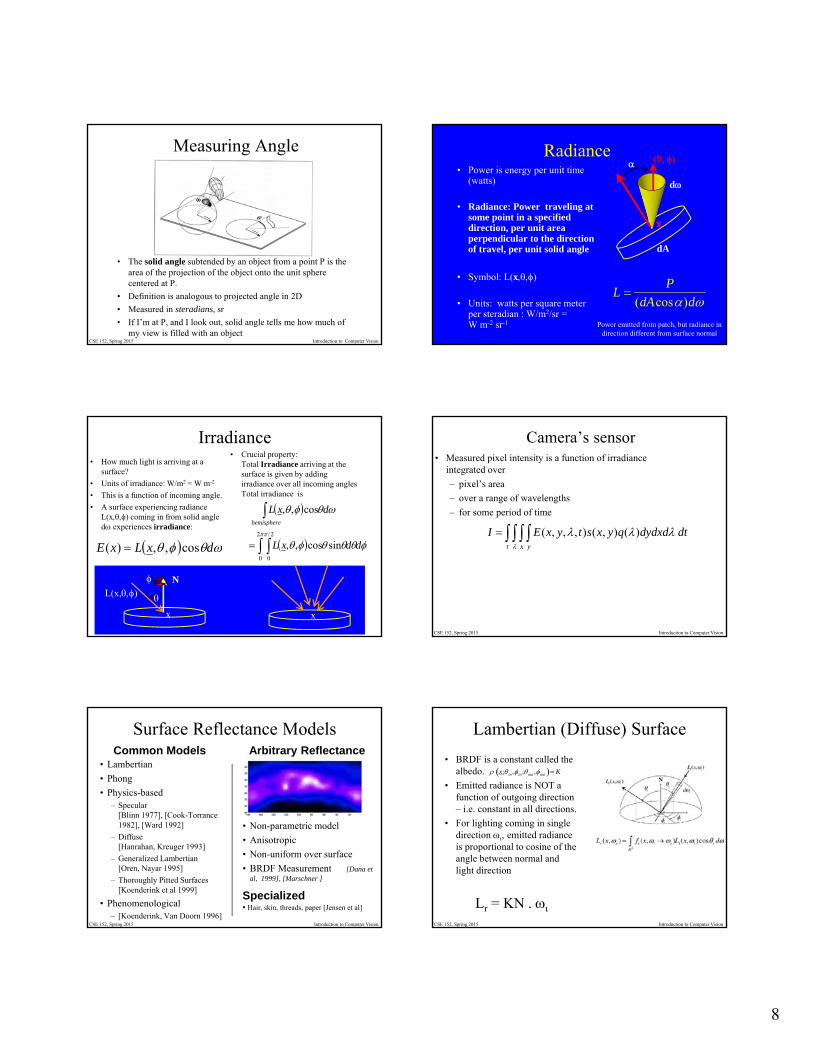
Measuring Angle

• The solid angle subtended by an object from a point P is the area of the projection of the object onto the unit sphere centered at P.

• Definition is analogous to projected angle in 2D

• Measured in steradians, sr

• If I’m at P, and I look out, solid angle tells me how much of my view is filled with an object

Radiance • Power is energy per unit time

(watts)

• Radiance: Power traveling at some point in a specified direction, per unit area perpendicular to the direction of travel, per unit solid angle

• Symbol: L(x

• Units: watts per square meter per steradian : W/m2/sr = W m-2 sr-1

L P

(dAcos)d

x

dA

d

Power emitted from patch, but radiance in direction different from surface normal

Irradiance• How much light is arriving at a

surface?

• Units of irradiance: W/m2 = W m-2

• This is a function of incoming angle.

• A surface experiencing radiance L(x) coming in from solid angle d experiences irradiance:

• Crucial property: Total Irradiance arriving at the surface is given by adding irradiance over all incoming angles Total irradiance is

dxLxE cos,,)(

2

0

2/

0

sincos,,

cos,,

ddxL

dxLhemisphere

NL(x,

x x


Camera’s sensor• Measured pixel intensity is a function of irradiance

integrated over

– pixel’s area

– over a range of wavelengths

– for some period of time

t x y

dtdydxdqyxstyxEI

)(),(),,,(


Surface Reflectance Models

• Lambertian

• Phong

• Physics-based– Specular

[Blinn 1977], [Cook-Torrance 1982], [Ward 1992]

– Diffuse [Hanrahan, Kreuger 1993]

– Generalized Lambertian [Oren, Nayar 1995]

– Thoroughly Pitted Surfaces [Koenderink et al 1999]

• Phenomenological– [Koenderink, Van Doorn 1996]

Common Models Arbitrary Reflectance

• Non-parametric model

• Anisotropic

• Non-uniform over surface

• BRDF Measurement [Dana et al, 1999], [Marschner ]

Specialized• Hair, skin, threads, paper [Jensen et al]


Lambertian (Diffuse) Surface

• BRDF is a constant called the albedo.

• Emitted radiance is NOT a function of outgoing direction – i.e. constant in all directions.

• For lighting coming in single direction , emitted radiance is proportional to cosine of the angle between normal and light direction

Lr = KN .

x; in, in;out,out K

9

CSE 152, Spring 2015 Introduction to Computer Vision CSE 152, Spring 2015 Introduction to Computer Vision

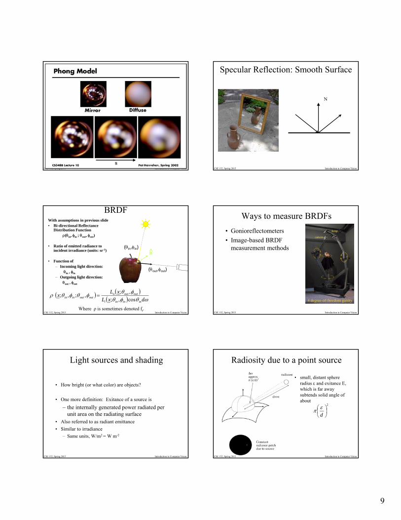
Specular Reflection: Smooth Surface

N


BRDFWith assumptions in previous slide• Bi-directional Reflectance

Distribution Function (in, in ; out, out)

• Ratio of emitted radiance to incident irradiance (units: sr-1)

• Function of– Incoming light direction:

in , in

– Outgoing light direction: out , out

dxL

xLx

ininini

outoutooutoutinin cos,;

,;,;,;

n(in,in)

(out,out)

Where ρ is sometimes denoted fr.CSE 152, Spring 2015 Introduction to Computer Vision

Ways to measure BRDFs

• Gonioreflectometers

• Image-based BRDF measurement methods


Light sources and shading

• How bright (or what color) are objects?

• One more definition: Exitance of a source is

– the internally generated power radiated per unit area on the radiating surface

• Also referred to as radiant emittance

• Similar to irradiance

– Same units, W/m2 = W m-2


Radiosity due to a point source

• small, distant sphere radius and exitance E, which is far away subtends solid angle of about

2

d

10


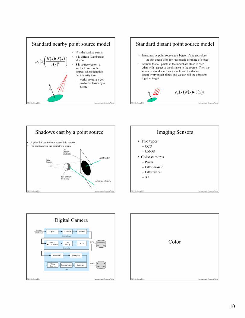
Standard nearby point source model

• N is the surface normal

• is diffuse (Lambertian) albedo

• S is source vector - a vector from x to the source, whose length is the intensity term

– works because a dot-product is basically a cosine

2xr

xSxNxd

NS


Standard distant point source model

• Issue: nearby point source gets bigger if one gets closer

– the sun doesn’t for any reasonable meaning of closer

• Assume that all points in the model are close to each other with respect to the distance to the source. Then the source vector doesn’t vary much, and the distance doesn’t vary much either, and we can roll the constants together to get:

xSxNxd N

S


Shadows cast by a point source

• A point that can’t see the source is in shadow

• For point sources, the geometry is simple

Cast Shadow

Attached Shadow


Imaging Sensors

• Two types– CCD

– CMOS

• Color cameras– Prism

– Filter mosaic

– Filter wheel

– X3


Digital Camera


Color

11


The appearance of colors

• Color appearance is strongly affected by (at least):– Spectrum of lighting striking the retina

– other nearby colors (space)

– adaptation to previous views (time)

– “state of mind”


Talking about colors

1. Spectrum –• A positive function over interval 400nm-

700nm

• “Infinite” number of values needed.

2. Names • red, harvest gold, cyan, aquamarine, auburn,

chestnut

• A large, discrete set of color names

3. R,G,B values • Just 3 numbers


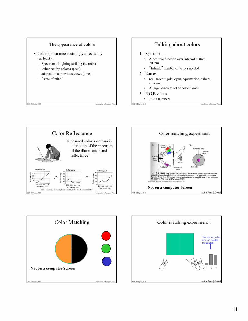
Color ReflectanceMeasured color spectrum is

a function of the spectrum of the illumination and reflectance

From Foundations of Vision, Brian Wandell, 1995, via B. Freeman slides

CSE 152, Spring 2015 Introduction to Computer Visionslide from T. Darrel

Not on a computer Screen


Color Matching

Not on a computer Screen

CSE 152, Spring 2015 Introduction to Computer Visionslide from T. Darrel

12

CSE 152, Spring 2015 Introduction to Computer Visionslide from T. Darrel CSE 152, Spring 2015 Introduction to Computer Vision

Color matching functions

• Choose primaries, say P1 P2, P3• For monochromatic (single wavelength) energy

function, what amounts of primaries will match it?

• i.e., For each wavelength , determine how much of A, of B, and of C is needed to match light of that wavelength alone.

• These are color matching functions

)(

)(

)(

c

b

a


RGB: primaries are monochromatic, energies are 645.2nm, 526.3nm, 444.4nm. Color matching functions have negative parts -> some colors can be matched only subtractively.

RGB


CIE XYZ: Color matching functions are positive everywhere, but primaries are imaginary. Usually draw x, y, where x=X/(X+Y+Z)y=Y/(X+Y+Z)

CIE XYZ


Three types of cones: R,G,B

There are three types of conesS: Short wave lengths (Blue)M: Mid wave lengths (Green)L: Long wave lengths (Red)

• Three attributes to a color• Three numbers to describe a color

Response of k’th cone = k()E()d


Color spaces

• Linear color spaces describe colors as linear combinations of primaries

• Choice of primaries=choice of color matching functions=choice of color space

• Color matching functions, hence color descriptions, are all within linear transformations

• RGB: primaries are monochromatic, energies are 645.2nm, 526.3nm, 444.4nm. Color matching functions have negative parts -> some colors can be matched only subtractively.

• CIE XYZ: Color matching functions are positive everywhere, but primaries are imaginary. Usually draw x, y, wherex=X/(X+Y+Z)y=Y/(X+Y+Z)

13


CIE -XYZ and x-y


CIE xyY (Chromaticity Space)


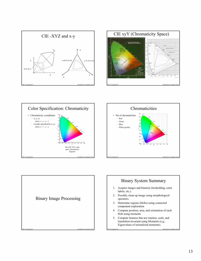
Color Specification: Chromaticity

• Chromaticity coordinates– (x, y, z)

where x + y + z = 1

– Usually specified by (x, y)where z = 1 – x – y

The CIE 1931 color space chromaticity

diagram


Chromaticities

• Set of chromaticities– Red

– Green

– Blue

– White (point)


Binary Image Processing


Binary System Summary

1. Acquire images and binarize (tresholding, color labels, etc.).

2. Possibly clean up image using morphological operators.

3. Determine regions (blobs) using connected component exploration

4. Compute position, area, and orientation of each blob using moments

5. Compute features that are rotation, scale, and translation invariant using Moments (e.g., Eigenvalues of normalized moments).

14


Threshold

T[ From Octavia Camps] CSE 152, Spring 2015 Introduction to Computer Vision

What is a region?

• “Maximal connected set of points in the image with same brightness value” (e.g., 1)

• Two points are connected if there exists a continuous path joining them.

• Regions can be simply connected (For every pair of points in the region, all smooth paths can be smoothly and continuously deformed into each other). Otherwise, region is multiply connected(holes)


Four & Eight Connectedness

Eight ConnectedFour Connected


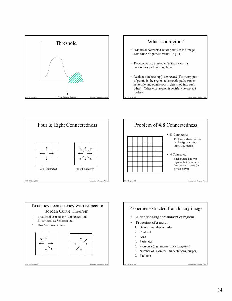
Problem of 4/8 Connectedness

1 1 1

1 1

1 1

1 1 1

• 8 Connected:– 1’s form a closed curve,

but background only forms one region.

• 4 Connected– Background has two

regions, but ones form four “open” curves (no closed curve)


To achieve consistency with respect to Jordan Curve Theorem

1. Treat background as 4-connected and foreground as 8-connected.

2. Use 6-connectedness


Properties extracted from binary image

• A tree showing containment of regions

• Properties of a region1. Genus – number of holes

2. Centroid

3. Area

4. Perimeter

5. Moments (e.g., measure of elongation)

6. Number of “extrema” (indentations, bulges)

7. Skeleton

15


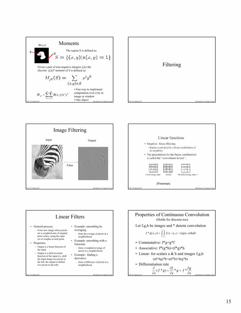
Moments

1 0

Given a pair of non-negative integers (j,k) the discrete (j,k)th moment of S is defined as:

B(x,y)

n

x

m

y

kjjk yxyxBM

1 1

),(

• Fast way to implement computation over n by m image or window• One object

The region S is defined as:

B


Filtering


Image Filtering

Input Output

Filter


(Freeman)


Linear Filters

• General process:– Form new image whose pixels

are a weighted sum of original pixel values, using the same set of weights at each point.

• Properties– Output is a linear function of

the input

– Output is a shift-invariant function of the input (i.e. shift the input image two pixels to the left, the output is shifted two pixels to the left)

• Example: smoothing by averaging– form the average of pixels in a

neighborhood

• Example: smoothing with a Gaussian– form a weighted average of

pixels in a neighborhood

• Example: finding a derivative– form a difference of pixels in a

neighborhood


Properties of Continuous Convolution(Holds for discrete too)

Let f,g,h be images and * denote convolution

• Commutative: f*g=g*f

• Associative: f*(g*h)=(f*g)*h

• Linear: for scalars a & b and images f,g,h(af+bg)*h=a(f*h)+b(g*h)

• Differentiation rule

x

gfg

x

fgf

x

**)*(

dudvvugvyuxfyxgf ),(),(),(*

16


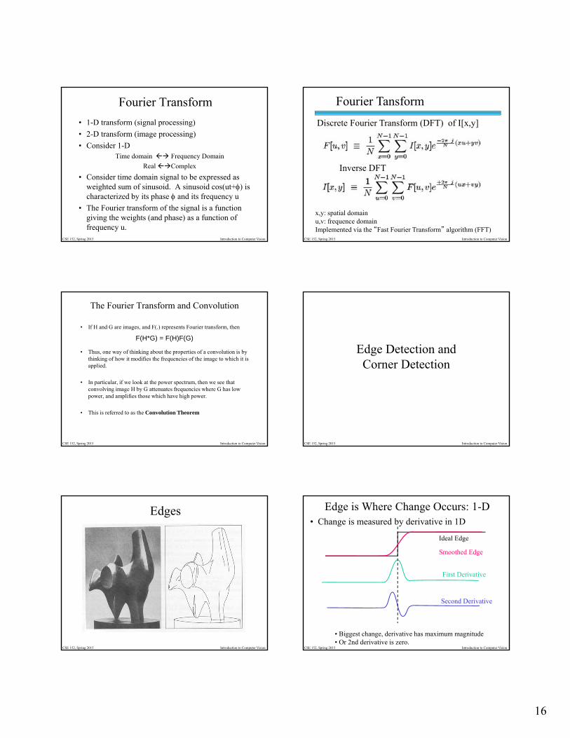
Fourier Transform

• 1-D transform (signal processing)

• 2-D transform (image processing)

• Consider 1-DTime domain Frequency Domain

Real Complex

• Consider time domain signal to be expressed as weighted sum of sinusoid. A sinusoid cos(ut+) is characterized by its phase and its frequency u

• The Fourier transform of the signal is a function giving the weights (and phase) as a function of frequency u.


Fourier Tansform

Discrete Fourier Transform (DFT) of I[x,y]

Inverse DFT

x,y: spatial domainu,v: frequence domainImplemented via the “Fast Fourier Transform” algorithm (FFT)


The Fourier Transform and Convolution

• If H and G are images, and F(.) represents Fourier transform, then

• Thus, one way of thinking about the properties of a convolution is by thinking of how it modifies the frequencies of the image to which it is applied.

• In particular, if we look at the power spectrum, then we see that convolving image H by G attenuates frequencies where G has low power, and amplifies those which have high power.

• This is referred to as the Convolution Theorem

F(H*G) = F(H)F(G)


Edge Detection andCorner Detection


Edges


Edge is Where Change Occurs: 1-D• Change is measured by derivative in 1D

Smoothed Edge

First Derivative

Second Derivative

Ideal Edge

• Biggest change, derivative has maximum magnitude• Or 2nd derivative is zero.

17


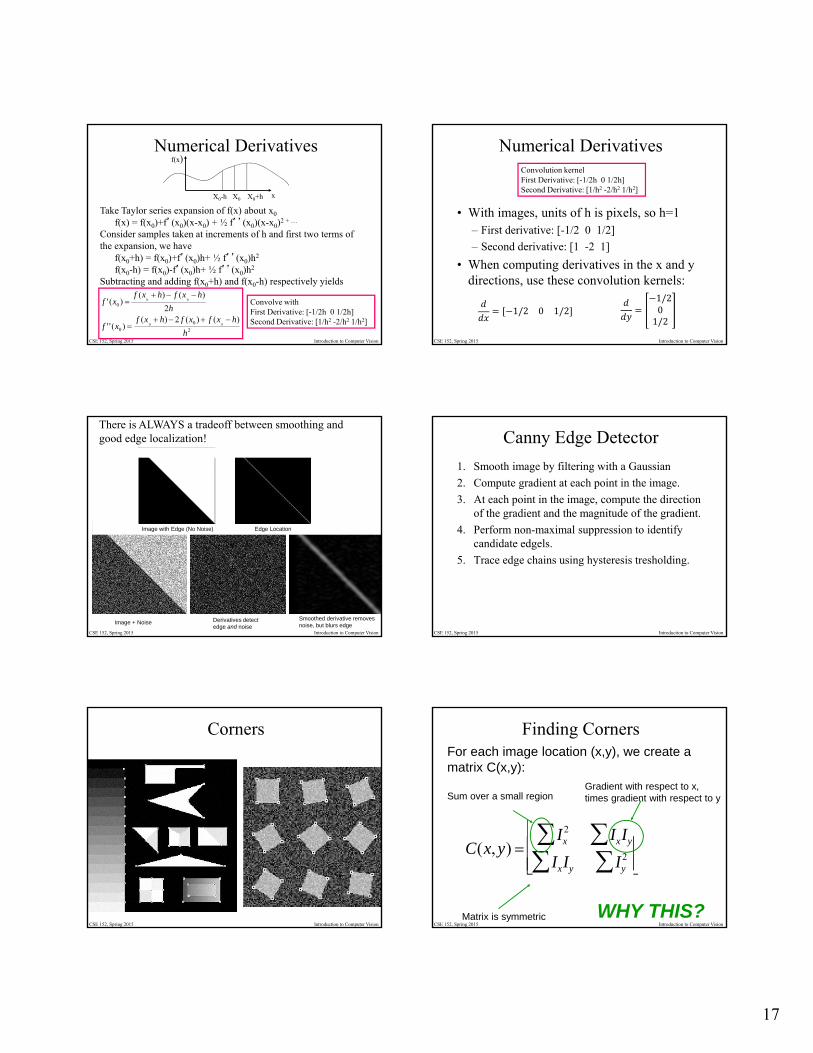
Numerical Derivativesf(x)

xX0 X0+hX0-h

Take Taylor series expansion of f(x) about x0

f(x) = f(x0)+f’(x0)(x-x0) + ½ f’’(x0)(x-x0)2 + …

Consider samples taken at increments of h and first two terms of the expansion, we have

f(x0+h) = f(x0)+f’(x0)h+ ½ f’’(x0)h2

f(x0-h) = f(x0)-f’(x0)h+ ½ f’’(x0)h2

Subtracting and adding f(x0+h) and f(x0-h) respectively yields

2

00

0

)()(2)()(''

2

)()()('

00

00

h

hxfxfhxfxf

h

hxfhxfxf

Convolve with

First Derivative: [-1/2h 0 1/2h]Second Derivative: [1/h2 -2/h2 1/h2]


Numerical Derivatives

• With images, units of h is pixels, so h=1– First derivative: [-1/2 0 1/2]

– Second derivative: [1 -2 1]

• When computing derivatives in the x and y directions, use these convolution kernels:

Convolution kernelFirst Derivative: [-1/2h 0 1/2h]Second Derivative: [1/h2 -2/h2 1/h2]

1/201/2

1/2 0 1/2


There is ALWAYS a tradeoff between smoothing and good edge localization!

Image with Edge (No Noise) Edge Location

Image + Noise Derivatives detect edge and noise

Smoothed derivative removes noise, but blurs edge


Canny Edge Detector

1. Smooth image by filtering with a Gaussian

2. Compute gradient at each point in the image.

3. At each point in the image, compute the direction of the gradient and the magnitude of the gradient.

4. Perform non-maximal suppression to identify candidate edgels.

5. Trace edge chains using hysteresis tresholding.


Corners


Finding Corners

C(x, y) Ix

2 IxIyIxIy Iy

2

For each image location (x,y), we create a matrix C(x,y):

Sum over a small regionGradient with respect to x, times gradient with respect to y

Matrix is symmetric WHY THIS?

18


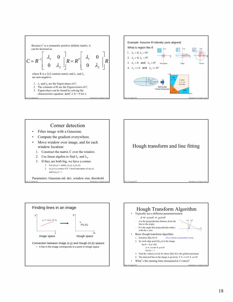
Because C is a symmetric positive definite matrix, it can be factored as:

C R1 1 0

0 2

R RT 1 0

0 2

R

where R is a 2x2 rotation matrix and λ1 and λ2

are non-negative.

1. λ1 and λ2 are the Eigenvalues of C. 2. The columns of R are the Eigenvectors of C.3. Eigenvalues can be found by solving the

characteristic equation det(C-λ I) = 0 for λ.CSE 152, Spring 2015 Introduction to Computer Vision

Example: Assume R=Identity (axis aligned)

What is region like if:

and

and


Corner detection• Filter image with a Gaussian.

• Compute the gradient everywhere.

• Move window over image, and for each window location:

1. Construct the matrix C over the window.

2. Use linear algebra to find and 3. If they are both big, we have a corner.

1. Let e(x,y) = min((x,y), (x,y)2. (x,y) is a corner if it’s local maximum of e(x,y)

and e(x,y) >

Parameters: Gaussian std. dev, window size, threshold CSE 152, Spring 2015 Introduction to Computer Vision

Hough transform and line fitting

Finding lines in an image

Connection between image (x,y) and Hough (m,b) spaces• A line in the image corresponds to a point in Hough space

x

y

m

b

(m0,b0)

image space Hough space


• Typically use a different parameterization

– d is the perpendicular distance from the line to the origin

– is the angle this perpendicular makes with the x axis

• Basic Hough transform algorithm1. Initialize H[d, ]=0 ; H is called accumulator array

2. for each edge point I[x,y] in the image

for = 0 to 180

H[d, ] += 1

3. Find the value(s) of (d, ) where H[d, ] is the global maximum

4. The detected line in the image is given by

• What’s the running time (measured in # votes)?

Hough Transform Algorithm

19


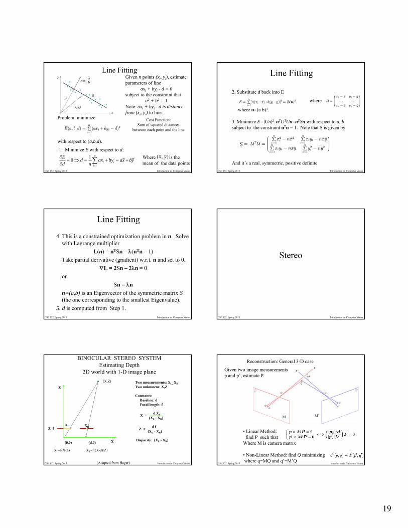
Line FittingGiven n points (xi, yi), estimate parameters of line

axi + byi - d = 0subject to the constraint that

a2 + b2 = 1Note: axi + byi - d is distance from (xi, yi) to line.

) ,( yx1. Minimize E with respect to d:

Where is themean of the data points

ybxabyaxn

dd

E n

iii

1

10

Problem: minimize

with respect to (a,b,d).

Cost Function:Sum of squared distances

between each point and the line

(xi,yi)


Line Fitting

2. Substitute d back into E

where n=(a b)T.

3. Minimize E=|Un|2=nTUTUn=nTSn with respect to a, bsubject to the constraint nTn = 1. Note that S is given by

And it’s a real, symmetric, positive definite

where

S =


Line Fitting

4. This is a constrained optimization problem in n. Solve with Lagrange multiplier

L(n) = nTSn – (nTn – 1)

Take partial derivative (gradient) w.r.t. n and set to 0.

L = 2Sn – n = 0

or

Sn = n

n=(a,b) is an Eigenvector of the symmetric matrix S(the one corresponding to the smallest Eigenvalue).

5. d is computed from Step 1.


Stereo


BINOCULAR STEREO SYSTEMEstimating Depth

2D world with 1-D image plane

Two measurements: XL, XR

Two unknowns: X,Z

Constants:Baseline: dFocal length: f

Disparity: (XL - XR)

Z = d f

(XL - XR)

X = d XL

(XL - XR)

(Adapted from Hager)

Z

X(0,0) (d,0)

Z=f

(X,Z)

XL XR

XL=f(X/Z) XR=f((X-d)/Z)


Reconstruction: General 3-D case

• Linear Method: find P such that

Where M is camera matrix

• Non-Linear Method: find Q minimizingwhere q=MQ and q’=M’Q

Given two image measurements p and p’, estimate P.

M M’

20


Need for correspondence

Truco Fig. 7.5


Where does a point in the left image match in the right image?

Nalwa Fig. 7.5


Epipolar Constraint

• Potential matches for p have to lie on the corresponding epipolar line l’.

• Potential matches for p’ have to lie on the corresponding epipolar line l.


Epipolar Geometry

• Epipolar Plane

• Epipoles • Epipolar Lines

• Baseline


Epipolar Constraint: Calibrated Case

Essential Matrix(Longuet-Higgins, 1981)

The vectors Op, OO’, and O’p’ are coplanar


Properties of the Essential Matrix

• E p’ is the epipolar line associated with p’.

• ETp is the epipolar line associated with p.

• E e’=0 and ETe=0.

• E is singular (rank 2).

• E has two equal non-zero singular values(Huang and Faugeras, 1989).

T

T

21


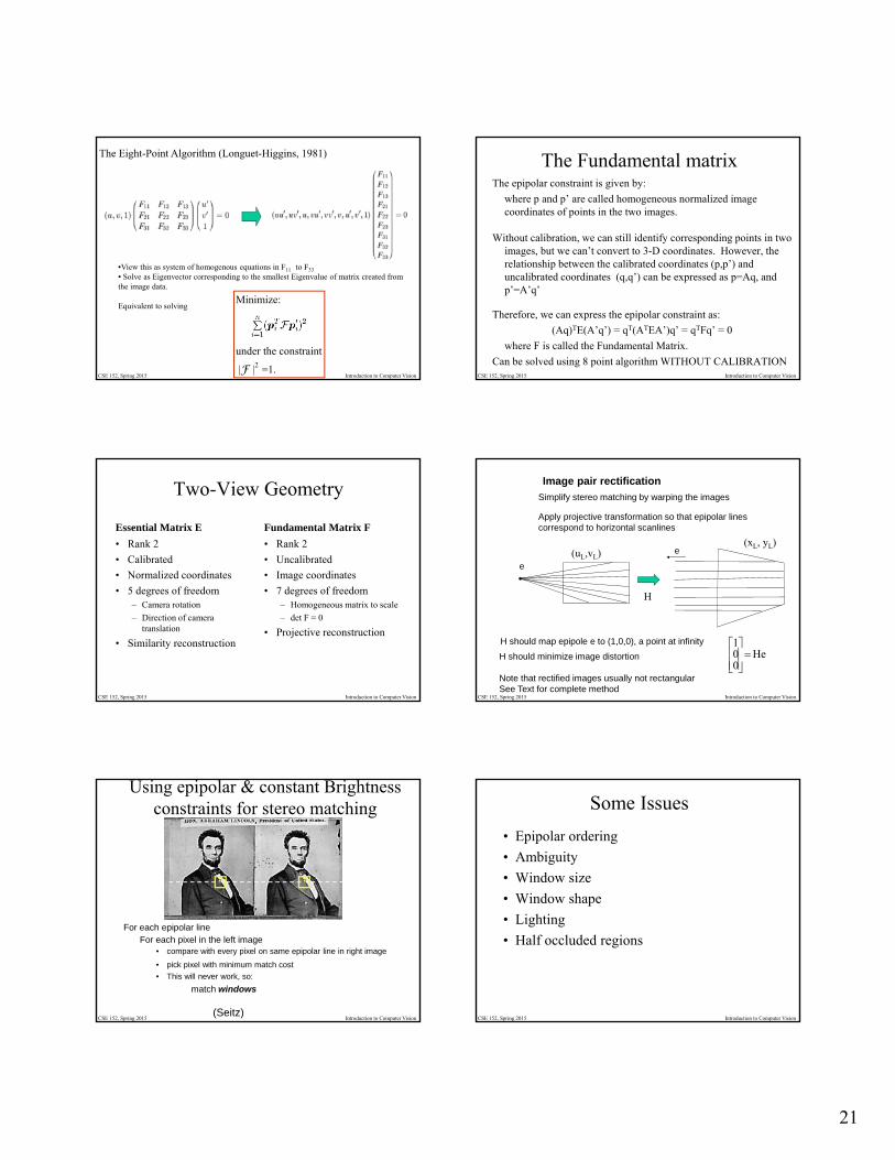
The Eight-Point Algorithm (Longuet-Higgins, 1981)

•View this as system of homogenous equations in F11 to F33

• Solve as Eigenvector corresponding to the smallest Eigenvalue of matrix created from the image data.

Equivalent to solving

|F | =1.

Minimize:

under the constraint2


The Fundamental matrixThe epipolar constraint is given by:

where p and p’ are called homogeneous normalized image coordinates of points in the two images.

Without calibration, we can still identify corresponding points in two images, but we can’t convert to 3-D coordinates. However, the relationship between the calibrated coordinates (p,p’) and uncalibrated coordinates (q,q’) can be expressed as p=Aq, and p’=A’q’

Therefore, we can express the epipolar constraint as:

(Aq)TE(A’q’) = qT(ATEA’)q’ = qTFq’ = 0

where F is called the Fundamental Matrix.

Can be solved using 8 point algorithm WITHOUT CALIBRATION


Two-View Geometry

Essential Matrix E

• Rank 2

• Calibrated

• Normalized coordinates

• 5 degrees of freedom– Camera rotation

– Direction of camera translation

• Similarity reconstruction

Fundamental Matrix F

• Rank 2

• Uncalibrated

• Image coordinates

• 7 degrees of freedom– Homogeneous matrix to scale

– det F = 0

• Projective reconstruction


Image pair rectification

Simplify stereo matching by warping the images

Apply projective transformation so that epipolar linescorrespond to horizontal scanlines

e

H should map epipole e to (1,0,0), a point at infinity

H should minimize image distortion

Note that rectified images usually not rectangularSee Text for complete method

He001

(uL,vL) e(xL, yL)

H


Using epipolar & constant Brightness constraints for stereo matching

For each epipolar lineFor each pixel in the left image

• compare with every pixel on same epipolar line in right image

• pick pixel with minimum match cost

• This will never work, so:

match windows

(Seitz)CSE 152, Spring 2015 Introduction to Computer Vision

Some Issues

• Epipolar ordering

• Ambiguity

• Window size

• Window shape

• Lighting

• Half occluded regions

22


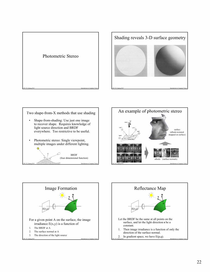
Photometric Stereo


Shading reveals 3-D surface geometry


Two shape-from-X methods that use shading

• Shape-from-shading: Use just one image to recover shape. Requires knowledge of light source direction and BRDF everywhere. Too restrictive to be useful.

• Photometric stereo: Single viewpoint, multiple images under different lighting.

BRDF(four dimensional function)


An example of photometric stereo

albedo (surface normals)

surface(albedo textured

mapped on surface)


Image Formation

For a given point A on the surface, the image irradiance E(x,y) is a function of

1. The BRDF at A

2. The surface normal at A

3. The direction of the light source

ns

a

E(x,y)

A


Reflectance Map

Let the BRDF be the same at all points on the surface, and let the light direction s be a constant.

1. Then image irradiance is a function of only the direction of the surface normal.

2. In gradient space, we have E(p,q).

ns

a

E(x,y)

23


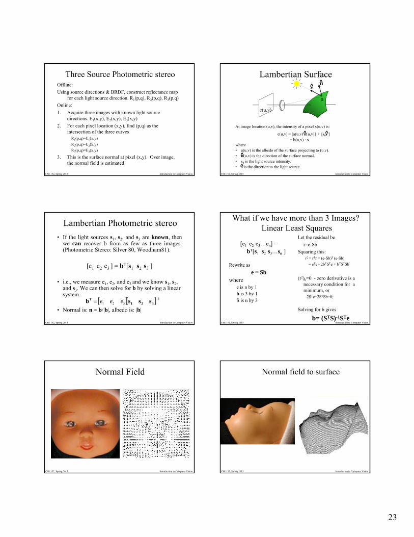
Three Source Photometric stereoOffline:

Using source directions & BRDF, construct reflectance map for each light source direction. R1(p,q), R2(p,q), R3(p,q)

Online:

1. Acquire three images with known light source directions. E1(x,y), E2(x,y), E3(x,y)

2. For each pixel location (x,y), find (p,q) as the intersection of the three curves

R1(p,q)=E1(x,y)

R2(p,q)=E2(x,y)

R3(p,q)=E3(x,y)

3. This is the surface normal at pixel (x,y). Over image, the normal field is estimated


Lambertian Surface

At image location (u,v), the intensity of a pixel x(u,v) is:

e(u,v) = [a(u,v) n(u,v)] · [s0s ]= b(u,v) · s

where• a(u,v) is the albedo of the surface projecting to (u,v).• n(u,v) is the direction of the surface normal.• s0 is the light source intensity.• s is the direction to the light source.

ns

^ ^

a

e(u,v)

^

^


Lambertian Photometric stereo

• If the light sources s1, s2, and s3 are known, thenwe can recover b from as few as three images.(Photometric Stereo: Silver 80, Woodham81).

[e1 e2 e3 ] = bT[s1 s2 s3 ]

• i.e., we measure e1, e2, and e3 and we know s1, s2, and s3. We can then solve for b by solving a linear system.

• Normal is: n = b/|b|, albedo is: |b|

1321

321T sssb eee


What if we have more than 3 Images?Linear Least Squares

[e1 e2 e3…en] =bT[s1 s2 s3…sn ]

Rewrite as

e = Sb where

e is n by 1b is 3 by 1S is n by 3

Let the residual be

r=e-Sb

Squaring this: r2 = rTr = (e-Sb)T (e-Sb)

= eTe - 2bTSTe + bTSTSb

(r2)b=0 - zero derivative is a necessary condition for a minimum, or-2STe+2STSb=0;

Solving for b gives

b= (STS)-1STe


Normal Field


Normal field to surface

24


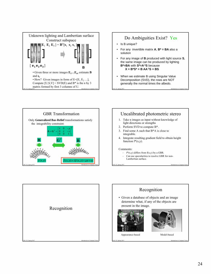
Unknown lighting and Lambertian surfaceConstruct subspace

[ ] [ ][ e1 e2 e3 ] B

• Given three or more images E1…En, estimate Band si.• How? Given images in form of E=[E1 E2 …], Compute [U,S,V] = SVD(E) and B* is the n by 3 matrix formed by first 3 columns of U.

[E1 E2 E3 ] = BT[s1 s2 s3 ]


Do Ambiguities Exist? Yes• Is B unique?

• For any invertible matrix A, B* = BA also a solution

• For any image of B produced with light source S, the same image can be produced by lighting B*=BA with S*=A-1S because

X = B*S* = B AA-1S = BS

• When we estimate B using Singular Value Decomposition (SVD), the rows are NOT generally the normal times the albedo.


GBR TransformationOnly Generalized Bas-Relief transformations satisfy

the integrability constraint:T

T

100

00

GA

B TG B

),( yxf yxyxfyxf ),(),(CSE 152, Spring 2015 Introduction to Computer Vision

Uncalibrated photometric stereo1. Take n images as input without knowledge of

light directions or strengths2. Perform SVD to compute B*.3. Find some A such that B*A is close to

integrable.4. Integrate resulting gradient field to obtain height

function f*(x,y).

Comments:– f*(x,y) differs from f(x,y) by a GBR.– Can use specularities to resolve GBR for non-

Lambertian surface.


Recognition


Recognition

• Given a database of objects and an image determine what, if any of the objects are present in the image.

Appearance-based Model-based

25


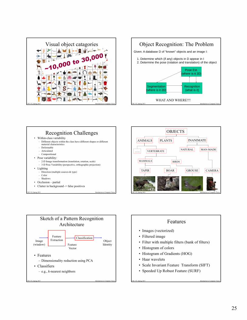
Visual object catagories


Object Recognition: The ProblemGiven: A database D of “known” objects and an image I:

1. Determine which (if any) objects in D appear in I2. Determine the pose (rotation and translation) of the object

Segmentation(where is it 2D)

Recognition(what is it)

Pose Est.(where is it 3D)

WHAT AND WHERE!!!


Recognition Challenges• Within-class variability

– Different objects within the class have different shapes or different material characteristics

– Deformable– Articulated– Compositional

• Pose variability: – 2-D Image transformation (translation, rotation, scale)– 3-D Pose Variability (perspective, orthographic projection)

• Lighting– Direction (multiple sources & type)– Color– Shadows

• Occlusion – partial• Clutter in background -> false positives


OBJECTS

ANIMALS INANIMATEPLANTS

MAN-MADENATURALVERTEBRATE…..

MAMMALS BIRDS

GROUSEBOARTAPIR CAMERA


Sketch of a Pattern Recognition Architecture

• Features– Dimensionality reduction using PCA

• Classifiers– e.g., k-nearest neighbors

FeatureExtraction

ClassificationImage

(window)ObjectIdentityFeature

Vector


Features

• Images (vectorized)

• Filtered image

• Filter with multiple filters (bank of filters)

• Histogram of colors

• Histogram of Gradients (HOG)

• Haar wavelets

• Scale Invariant Feature Transform (SIFT)

• Speeded Up Robust Feature (SURF)

26


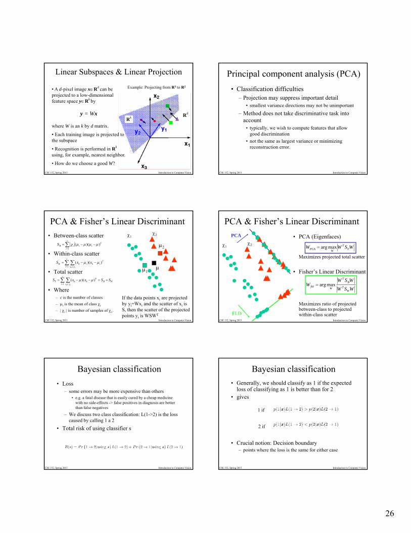
Linear Subspaces & Linear Projection

• A d-pixel image xRd can be projected to a low-dimensional feature space yRk by

y = Wx

where W is an k by d matrix.

• Each training image is projected to the subspace

• Recognition is performed in Rk

using, for example, nearest neighbor.

• How do we choose a good W?

Example: Projecting from R3 to R2

Rk Rd


Principal component analysis (PCA)

• Classification difficulties– Projection may suppress important detail

• smallest variance directions may not be unimportant

– Method does not take discriminative task into account

• typically, we wish to compute features that allow good discrimination

• not the same as largest variance or minimizing reconstruction error.


PCA & Fisher’s Linear Discriminant

• Between-class scatter

• Within-class scatter

• Total scatter

• Where– c is the number of classes

– i is the mean of class i

– | i | is number of samples of i..

Tii

c

iiBS ))((

1

c

i x

TikikW

ik

xxS1

))((

WB

c

i x

TkkT SSxxS

ik

1

))((

1

2

12

If the data points xi are projected by yi=Wxi and the scatter of xi is S, then the scatter of the projected points yi is WSWT


PCA & Fisher’s Linear Discriminant

• PCA (Eigenfaces)

Maximizes projected total scatter

• Fisher’s Linear Discriminant

Maximizes ratio of projected between-class to projected within-class scatter

WSWW TT

WPCA maxarg

WSW

WSWW

WT

BT

Wfld maxarg

12

PCA

FLD


Bayesian classification

• Loss– some errors may be more expensive than others

• e.g. a fatal disease that is easily cured by a cheap medicine with no side-effects -> false positives in diagnosis are better than false negatives

– We discuss two class classification: L(1->2) is the loss caused by calling 1 a 2

• Total risk of using classifier s


Bayesian classification

• Generally, we should classify as 1 if the expected loss of classifying as 1 is better than for 2

• gives

• Crucial notion: Decision boundary– points where the loss is the same for either case

1 if

2 if

27


• Classifier boils down to: choose class that

minimizes:

x, k 2 2 log k

where

x, k x

k T 1 x k

12

because covariance is common, this simplifies to sign ofa linear expression (i.e. Voronoi diagram in 2D for =I)

Mahalanobis distance


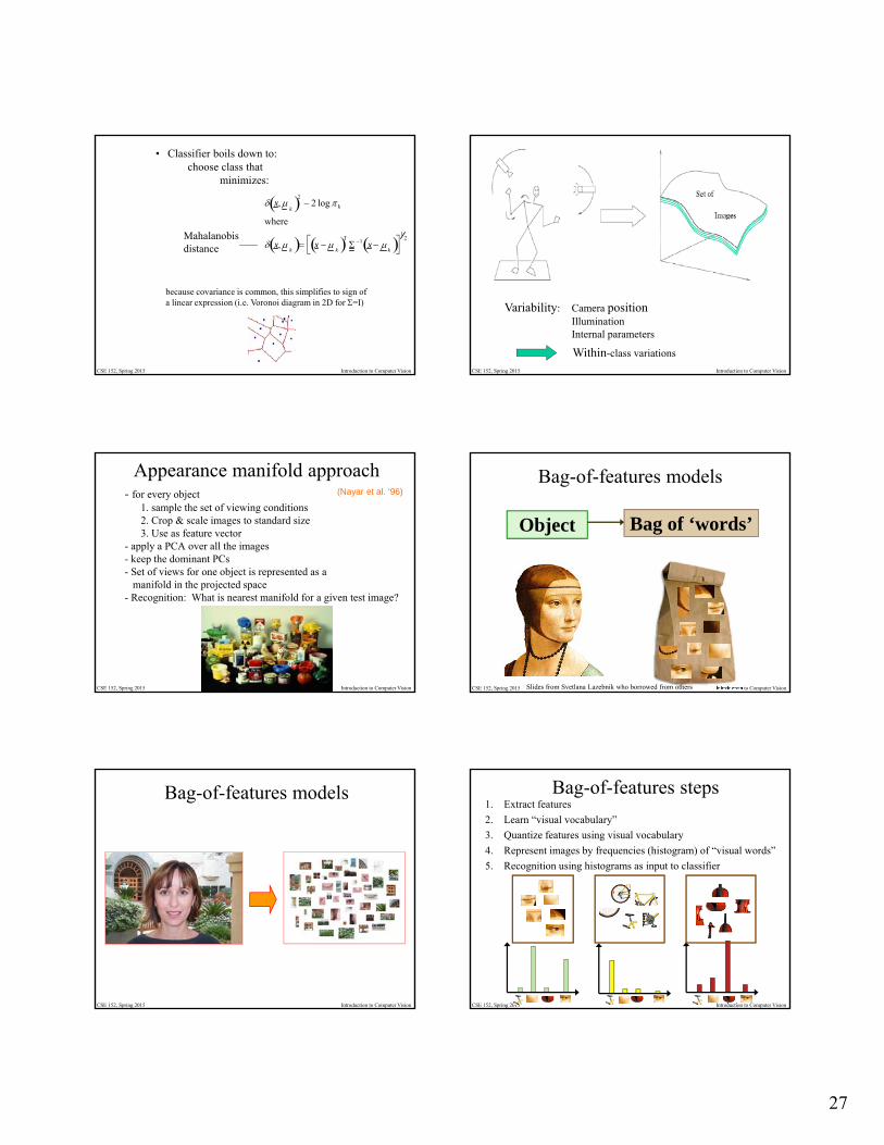
Variability: Camera positionIlluminationInternal parameters

Within-class variations


Appearance manifold approach- for every object

1. sample the set of viewing conditions2. Crop & scale images to standard size3. Use as feature vector

- apply a PCA over all the images - keep the dominant PCs- Set of views for one object is represented as a

manifold in the projected space- Recognition: What is nearest manifold for a given test image?

(Nayar et al. ‘96)


Object Bag of ‘words’

Bag-of-features models

Slides from Svetlana Lazebnik who borrowed from others


Bag-of-features models


1. Extract features

2. Learn “visual vocabulary”

3. Quantize features using visual vocabulary

4. Represent images by frequencies (histogram) of “visual words”

5. Recognition using histograms as input to classifier

Bag-of-features steps

28


Model-Based Recognition

• Given 3-D models of each object• Detect image features (often edges, line segments, conic sections)• Establish correspondence between model & image features• Estimate pose• Consistency of projected model with image.


Recognition by Hypothesize and Test

• General idea– Hypothesize object identity and

pose

– Recover camera parameters (widely known as backprojection)

– Render object using camera parameters

– Compare to image

• Issues– Where do the hypotheses come

from?

– How do we compare to image (verification)?

• Simplest approach– Construct a

correspondence for all object features to every correctly sized subset of image points

• These are the hypotheses

– Expensive search, which is also redundant.


Pose consistency

• Correspondences between image features and model features are not independent.

• A small number of correspondences yields a camera matrix --- the others correspondences must be consistent with this.

• Strategy:– Generate hypotheses

using small numbers of correspondences (e.g., triples of points for a calibrated perspective camera)

– Backproject and verify


Voting on Pose

• Each model leads to many correct sets of correspondences, each of which has the same pose– Vote on pose, in an accumulator array (similar

to a Hough transform accumulator array)


Invariance

• Properties or measures that are independent of some group of transformation (e.g., rigid, affine, projective, etc.)

• For example, under affine transformations:– Collinearity

– Parallelism

– Intersection

– Distance ratio along a line

– Angle ratios of three intersecting lines

– Affine coordinates


Geometric hashing

• Vote on identity and correspondence using invariants– Take hypotheses with large enough votes

• Building a table (affine example):– Take all triplets of points in on model image to

be base points P1, P2, P3.– Take every fourth point and compute ’s– Fill up a table, indexed by ’s, with

• the base points and fourth point that yield those ’s• the object identity

29


Recognition using local image features

• Detect corners in image (e.g. Harris corner detector).

• Represent neighborhood of corner by a feature vector produced by Gabor Filters, K-jets, affine-invariant features, etc.).

• Modeling: Given an training image of an object w/o clutter, detect corners, compute feature descriptors, store these.

• Recognition time: Given test image with possible clutter, detect corners and compute features. Find models with same feature descriptors (hashing) and vote.


Local image features + spatial relationships

Figure from “Local grayvalue invariants for image retrieval,” by C. Schmid and R. Mohr, IEEE Trans. Pattern Analysis and Machine Intelligence, 1997 copyright 1997, IEEE


Motion


Structure-from-Motion (SFM)Goal: Take as input two or more images or

video without knowledge of the camera position/motion, and estimate the camera position and 3D structure of scene.

Two Approaches1. Discrete motion (wide baseline)

1. Orthographic (affine) vs. Perspective2. Two view vs. Multi-view3. Calibrated vs. Uncalibrated

2. Continuous (Infinitesimal) motion


Two-view discrete motion(same as stereo)

Input: Two images1. Detect feature points2. Find 8 matching feature points (easier said than

done)3. Compute the Essential Matrix E using Normalized

8-point Algorithm4. Compute R and T (recall that E=RS where S is

skew symmetric matrix)5. Perform stereo matching using recovered epipolar

geometry expressed via E.6. Reconstruct 3-D geometry of corresponding points.


Continuous motion using motion fields

30


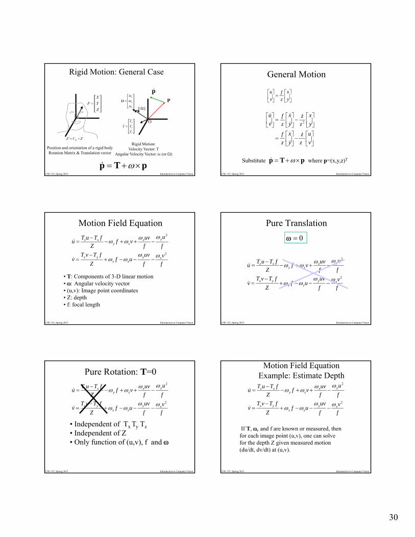
Rigid Motion: General Case

Position and orientation of a rigid bodyRotation Matrix & Translation vector

Rigid Motion:Velocity Vector: T

Angular Velocity Vector: (or )

P

pTp

p


General Motion

y

x

z

f

v

u

y

x

z

z

y

x

z

f

v

u2

v

u

z

z

y

x

z

f

pTp Substitute where p=(x,y,z)T


Motion Field Equation

• T: Components of 3-D linear motion• Angular velocity vector• (u,v): Image point coordinates• Z: depth• f: focal length

f

v

f

uvuf

Z

fTvTv

f

u

f

uvvf

Z

fTuTu

xyzx

yz

yxzy

xz

2

2


f

v

f

uvuf

Z

fTvTv

f

u

f

uvvf

Z

fTuTu

xyzx

yz

yxzy

xz

2

2

Pure Translation


Pure Rotation: T=0

• Independent of Tx Ty Tz

• Independent of Z• Only function of (u,v), f and

f

v

f

uvuf

Z

fTvTv

f

u

f

uvvf

Z

fTuTu

xyzx

yz

yxzy

xz

2

2


Motion Field EquationExample: Estimate Depth

If T, and f are known or measured, then for each image point (u,v), one can solve for the depth Z given measured motion (du/dt, dv/dt) at (u,v).

f

v

f

uvuf

Z

fTvTv

f

u

f

uvvf

Z

fTuTu

xyzx

yz

yxzy

xz

2

2

31


Optical Flow


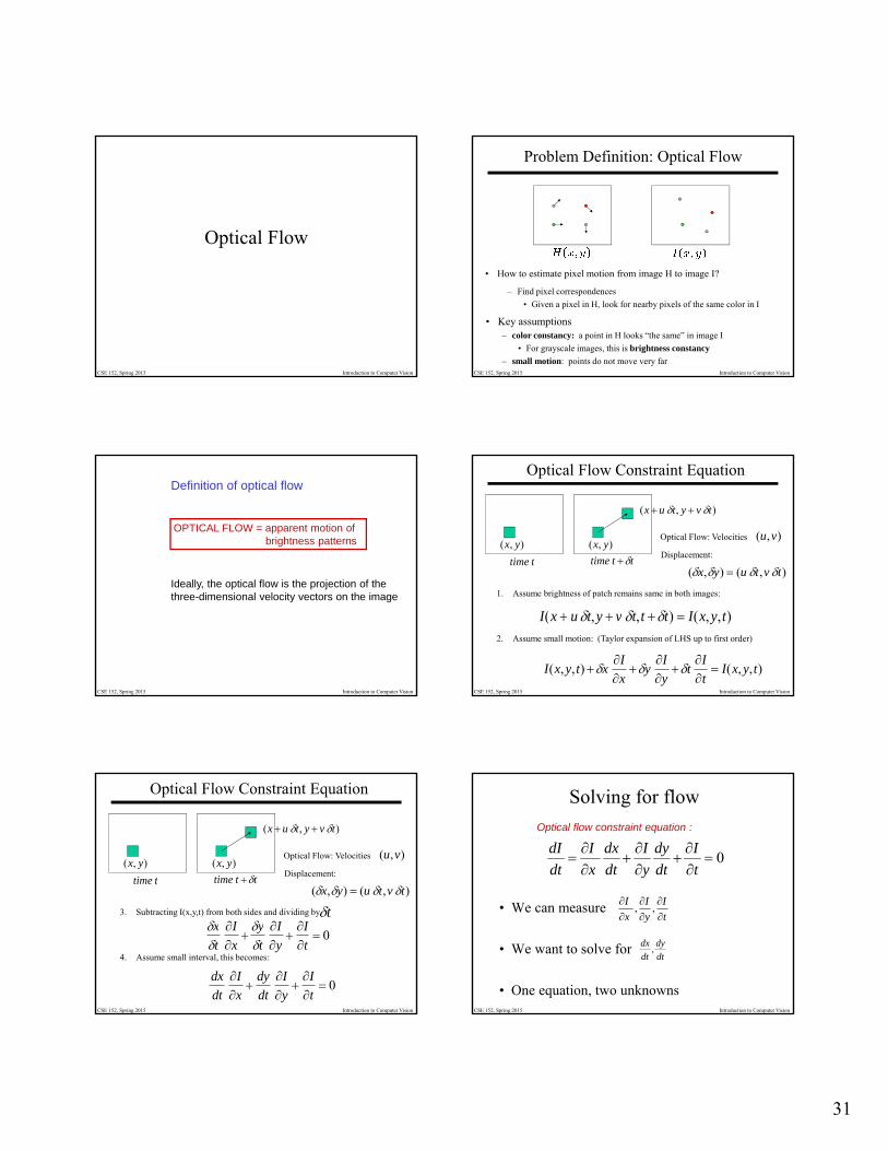
Problem Definition: Optical Flow

• How to estimate pixel motion from image H to image I?

– Find pixel correspondences

• Given a pixel in H, look for nearby pixels of the same color in I

• Key assumptions– color constancy: a point in H looks “the same” in image I

• For grayscale images, this is brightness constancy

– small motion: points do not move very far


Definition of optical flow

OPTICAL FLOW = apparent motion of brightness patterns

Ideally, the optical flow is the projection of the three-dimensional velocity vectors on the image


Optical Flow Constraint Equation

1. Assume brightness of patch remains same in both images:

2. Assume small motion: (Taylor expansion of LHS up to first order)

),( yx

),( tvytux

ttime tttime ),( yx

Optical Flow: Velocities ),( vu

Displacement:

),(),( tvtuyx

I(x u t,y v t,t t) I(x, y,t)

I(x, y, t) xI

xy

I

yt

I

t I(x, y,t)


Optical Flow Constraint Equation

),( yx

),( tvytux

ttime tttime ),( yx

Optical Flow: Velocities ),( vu

Displacement:

),(),( tvtuyx

x

t

I

xy

t

I

yI

t 0

3. Subtracting I(x,y,t) from both sides and dividing by t

4. Assume small interval, this becomes:

dx

dt

I

x

dy

dt

I

yI

t 0


Solving for flow

• We can measure

• We want to solve for

• One equation, two unknowns

Optical flow constraint equation :

0

t

I

dt

dy

y

I

dt

dx

x

I

dt

dI

t

I

y

I

x

I

,,

dt

dy

dt

dx,

32


02),(

02),(

tyxy

tyxx

IvIuIIdv

vudE

IvIuIIdu

vudE



Edge

– large gradients, all the same– large 1, small 2


Low texture region

– gradients have small magnitude– small 1, small 2


High textured region

– gradients are different, large magnitudes– large 1, large 2


Revisiting the small motion assumption

• Is this motion small enough?– Probably not—it’s much larger than one pixel (2nd order terms dominate)

– How might we solve this problem?

33

CSE 152, Spring 2015 Introduction to Computer Vision CSE 152, Spring 2015 Introduction to Computer Vision

Final exam

• Final exam is a take home exam– Will be distributed night of Monday, June 8

– Due Thursday, June 11, 10:00 PM

cse 152, spring 2015 introduction to computer...

Documents