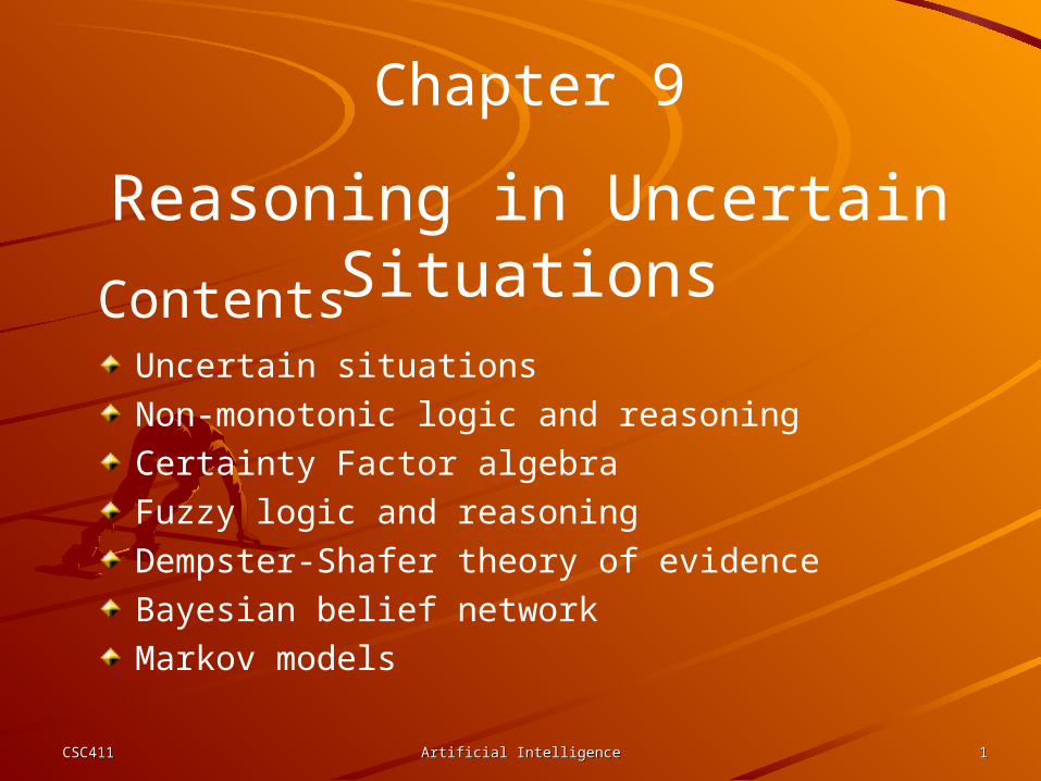
csc411artificial intelligence1 chapter 9 reasoning in uncertain situations contents uncertain...
TRANSCRIPT
CSC411CSC411 Artificial IntelligenceArtificial Intelligence 11
Chapter 9
Reasoning in Uncertain Situations
ContentsUncertain situationsNon-monotonic logic and reasoning Certainty Factor algebraFuzzy logic and reasoningDempster-Shafer theory of evidenceBayesian belief networkMarkov models
CSC411CSC411 Artificial IntelligenceArtificial Intelligence 22
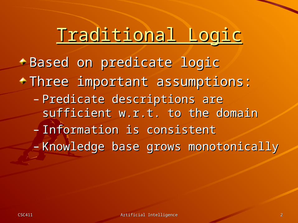
Traditional LogicTraditional Logic
Based on predicate logicBased on predicate logic
Three important assumptions:Three important assumptions:– Predicate descriptions are sufficient Predicate descriptions are sufficient
w.r.t. to the domainw.r.t. to the domain– Information is consistentInformation is consistent– Knowledge base grows monotonically Knowledge base grows monotonically
CSC411CSC411 Artificial IntelligenceArtificial Intelligence 33
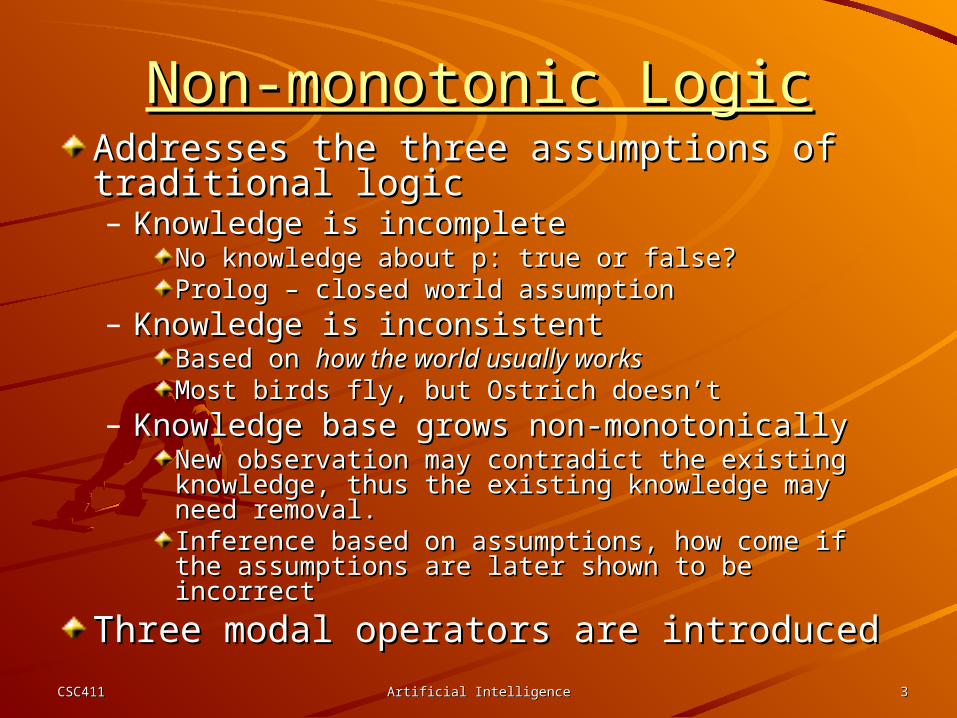
Non-monotonic LogicNon-monotonic LogicAddresses the three assumptions of Addresses the three assumptions of traditional logictraditional logic– Knowledge is incompleteKnowledge is incomplete
No knowledge about p: true or false?No knowledge about p: true or false?Prolog – closed world assumptionProlog – closed world assumption
– Knowledge is inconsistentKnowledge is inconsistentBased on Based on how the world usually workshow the world usually worksMost birds fly, but Ostrich doesn’tMost birds fly, but Ostrich doesn’t
– Knowledge base grows non-monotonicallyKnowledge base grows non-monotonicallyNew observation may contradict the existing New observation may contradict the existing knowledge, thus the existing knowledge may need knowledge, thus the existing knowledge may need removal. removal. Inference based on assumptions, how come if the Inference based on assumptions, how come if the assumptions are later shown to be incorrectassumptions are later shown to be incorrect
Three modal operators are introduced Three modal operators are introduced
CSC411CSC411 Artificial IntelligenceArtificial Intelligence 44
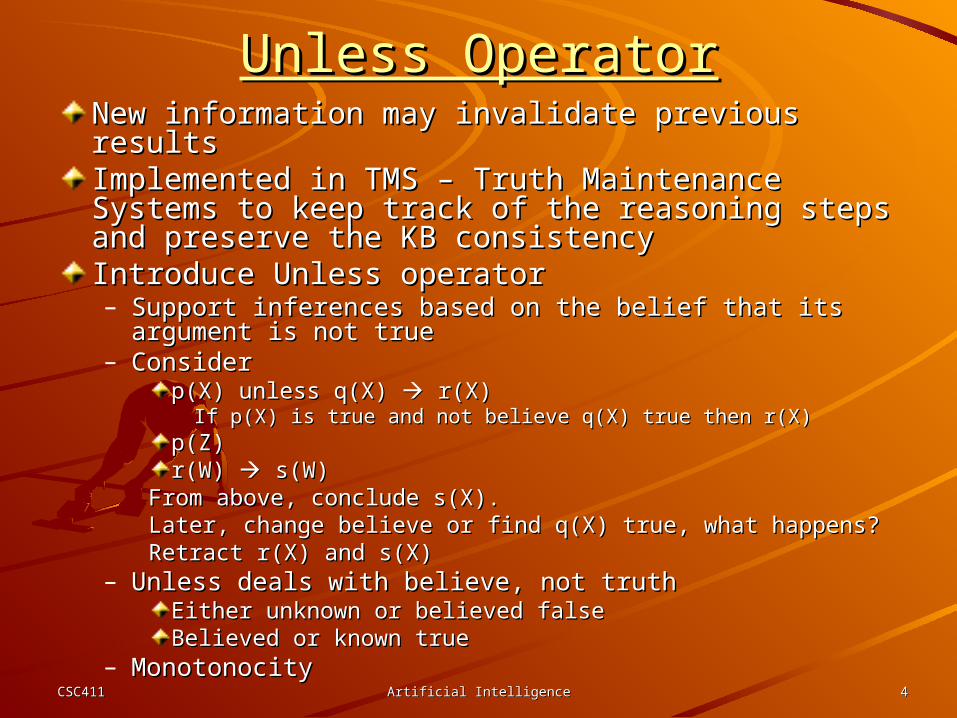
Unless OperatorUnless OperatorNew information may invalidate previous resultsNew information may invalidate previous resultsImplemented in TMS – Truth Maintenance Implemented in TMS – Truth Maintenance Systems to keep track of the reasoning steps and Systems to keep track of the reasoning steps and preserve the KB consistency preserve the KB consistency Introduce Unless operatorIntroduce Unless operator– Support inferences based on the belief that its argument Support inferences based on the belief that its argument
is not trueis not true– ConsiderConsider
p(X) unless q(X) p(X) unless q(X) r(X) r(X)If p(X) is true and not believe q(X) true then r(X)If p(X) is true and not believe q(X) true then r(X)
p(Z)p(Z)r(W) r(W) s(W) s(W)
From above, conclude s(X). From above, conclude s(X). Later, change believe or find q(X) true, what happens?Later, change believe or find q(X) true, what happens?Retract r(X) and s(X)Retract r(X) and s(X)
– Unless deals with believe, not truthUnless deals with believe, not truthEither unknown or believed falseEither unknown or believed falseBelieved or known trueBelieved or known true
– MonotonocityMonotonocity
CSC411CSC411 Artificial IntelligenceArtificial Intelligence 55
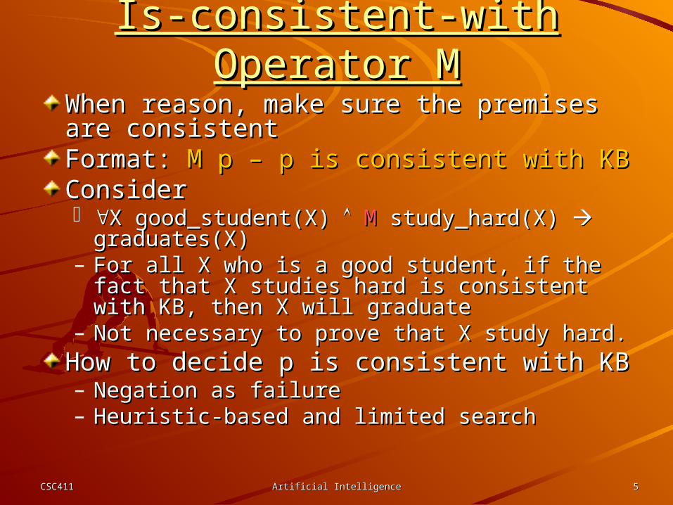
Is-consistent-with Operator MIs-consistent-with Operator MWhen reason, make sure the premises are When reason, make sure the premises are consistentconsistentFormat: Format: M p – p is consistent with KB M p – p is consistent with KB ConsiderConsider X good_student(X) X good_student(X) MM study_hard(X) study_hard(X)
graduates(X)graduates(X)– For all X who is a good student, if the fact that For all X who is a good student, if the fact that
X studies hard is consistent with KB, then X will X studies hard is consistent with KB, then X will graduategraduate
– Not necessary to prove that X study hard.Not necessary to prove that X study hard.How to decide p is consistent with KBHow to decide p is consistent with KB– Negation as failureNegation as failure– Heuristic-based and limited search Heuristic-based and limited search
CSC411CSC411 Artificial IntelligenceArtificial Intelligence 66
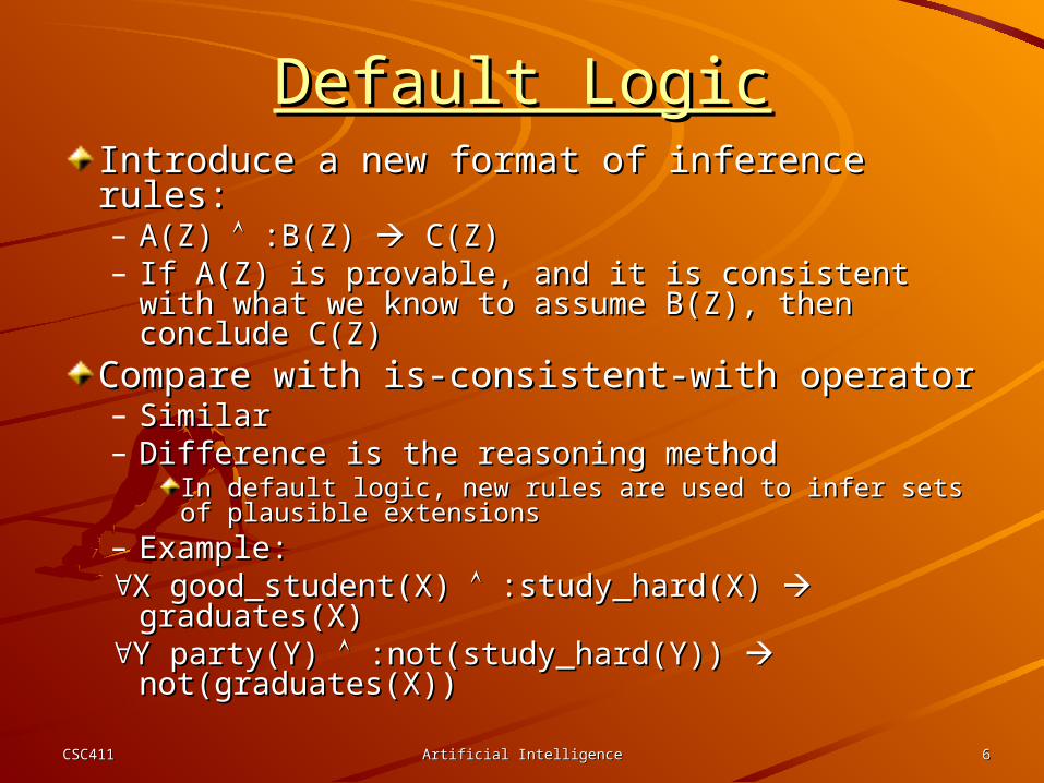
Default LogicDefault LogicIntroduce a new format of inference rules:Introduce a new format of inference rules:– A(Z) A(Z) :B(Z) :B(Z) C(Z) C(Z)– If A(Z) is provable, and it is consistent with If A(Z) is provable, and it is consistent with
what we know to assume B(Z), then conclude what we know to assume B(Z), then conclude C(Z)C(Z)
Compare with is-consistent-with operatorCompare with is-consistent-with operator– SimilarSimilar– Difference is the reasoning methodDifference is the reasoning method
In default logic, new rules are used to infer sets of In default logic, new rules are used to infer sets of plausible extensionsplausible extensions
– Example:Example:X good_student(X) X good_student(X) :study_hard(X) :study_hard(X)
graduates(X)graduates(X)Y party(Y) Y party(Y) :not(study_hard(Y)) :not(study_hard(Y))
not(graduates(X)) not(graduates(X))
CSC411CSC411 Artificial IntelligenceArtificial Intelligence 77
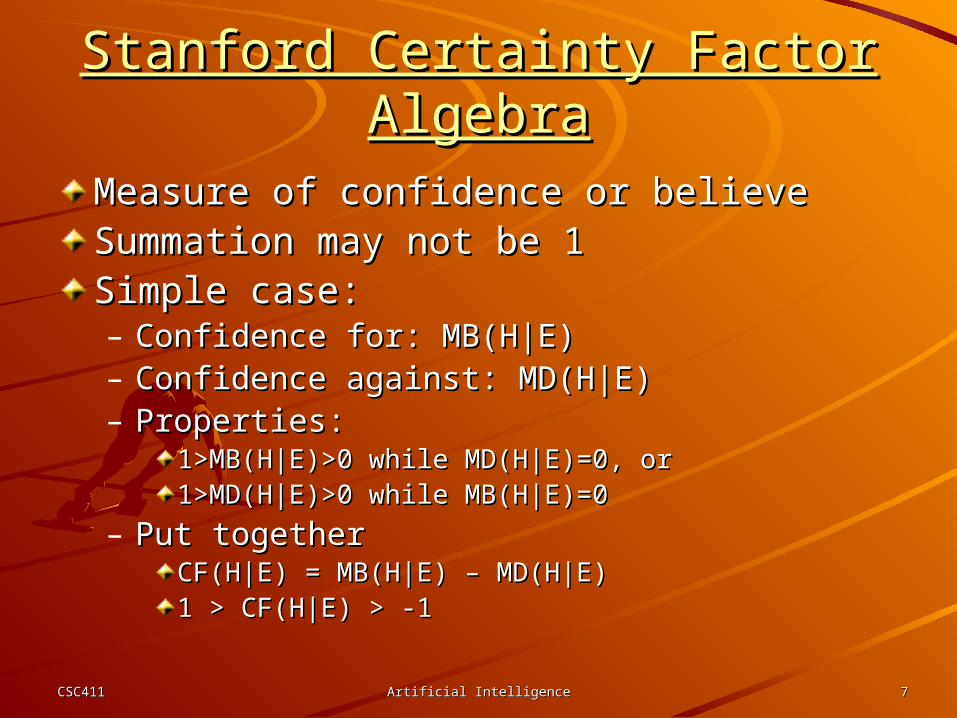
Stanford Certainty Factor AlgebraStanford Certainty Factor AlgebraMeasure of confidence or believeMeasure of confidence or believeSummation may not be 1Summation may not be 1Simple case:Simple case:– Confidence for: MB(H|E)Confidence for: MB(H|E)– Confidence against: MD(H|E)Confidence against: MD(H|E)– Properties:Properties:
1>MB(H|E)>0 while MD(H|E)=0, or1>MB(H|E)>0 while MD(H|E)=0, or1>MD(H|E)>0 while MB(H|E)=01>MD(H|E)>0 while MB(H|E)=0
– Put togetherPut togetherCF(H|E) = MB(H|E) – MD(H|E)CF(H|E) = MB(H|E) – MD(H|E)1 > CF(H|E) > -11 > CF(H|E) > -1
CSC411CSC411 Artificial IntelligenceArtificial Intelligence 88
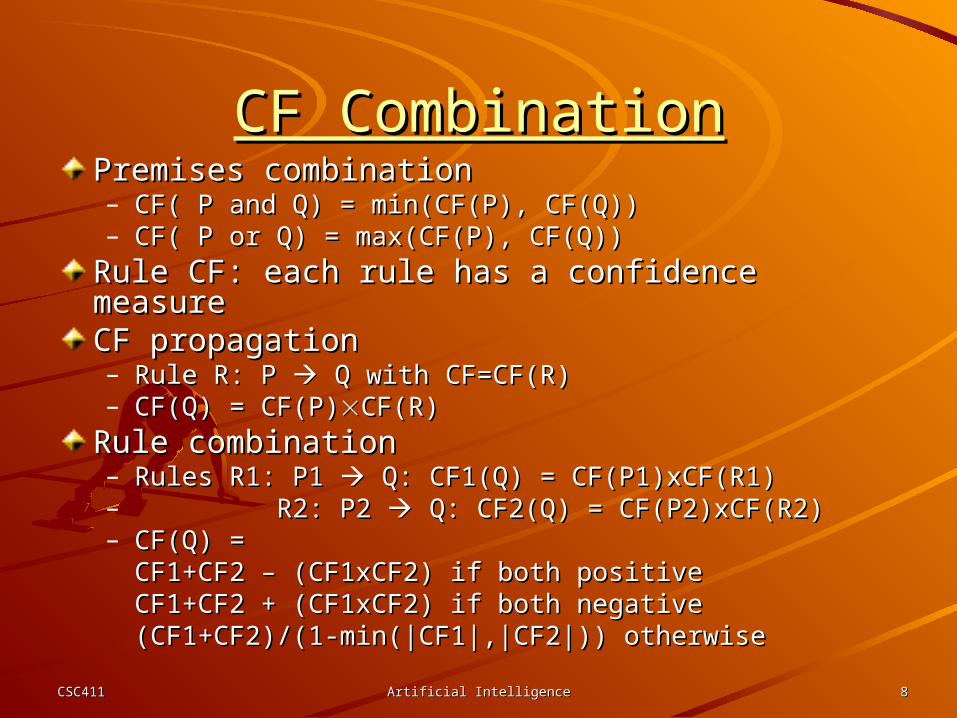
CF CombinationCF CombinationPremises combinationPremises combination– CF( P and Q) = min(CF(P), CF(Q))CF( P and Q) = min(CF(P), CF(Q))– CF( P or Q) = max(CF(P), CF(Q))CF( P or Q) = max(CF(P), CF(Q))
Rule CF: each rule has a confidence measureRule CF: each rule has a confidence measureCF propagationCF propagation– Rule R: P Rule R: P Q with CF=CF(R) Q with CF=CF(R)– CF(Q) = CF(P)CF(Q) = CF(P)CF(R)CF(R)
Rule combinationRule combination– Rules R1: P1 Rules R1: P1 Q: CF1(Q) = CF(P1)xCF(R1) Q: CF1(Q) = CF(P1)xCF(R1)– R2: P2 R2: P2 Q: CF2(Q) = CF(P2)xCF(R2) Q: CF2(Q) = CF(P2)xCF(R2)– CF(Q) =CF(Q) =
CF1+CF2 – (CF1xCF2) if both positiveCF1+CF2 – (CF1xCF2) if both positiveCF1+CF2 + (CF1xCF2) if both negativeCF1+CF2 + (CF1xCF2) if both negative(CF1+CF2)/(1-min(|CF1|,|CF2|)) otherwise(CF1+CF2)/(1-min(|CF1|,|CF2|)) otherwise
CSC411CSC411 Artificial IntelligenceArtificial Intelligence 99
Fuzzy SetsFuzzy SetsClassic setsClassic sets– Completeness: x in either A or ¬ACompleteness: x in either A or ¬A– Exclusive: can not be in both A and ¬AExclusive: can not be in both A and ¬AFuzzy setsFuzzy sets– Violate the two assumptionsViolate the two assumptions– Possibility theory -- measure of confidence or Possibility theory -- measure of confidence or
believebelieve– Probability theory – randomnessProbability theory – randomness– Process imprecisionProcess imprecision– Introduce membership functionIntroduce membership function– Believe xBelieve xA in some degree between 0 and 1, A in some degree between 0 and 1,
inclusiveinclusive
CSC411CSC411 Artificial IntelligenceArtificial Intelligence 1010
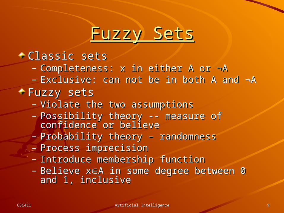
The fuzzy set representation for “small integers.”
CSC411CSC411 Artificial IntelligenceArtificial Intelligence 1111
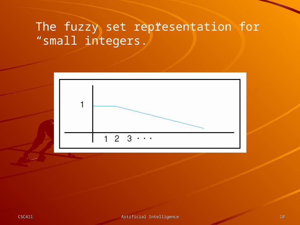
A fuzzy set representation for the sets short, medium, and tall males.
CSC411CSC411 Artificial IntelligenceArtificial Intelligence 1212
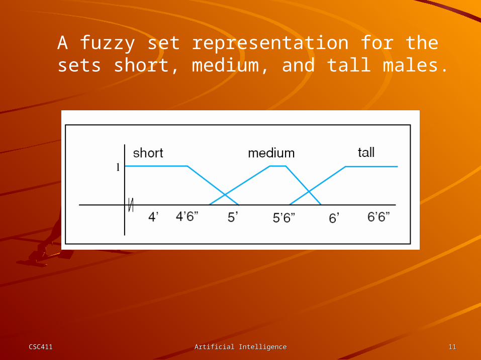
Fuzzy Set OperationsFuzzy Set OperationsFuzzy set operations are defined as the Fuzzy set operations are defined as the operations of membership functionsoperations of membership functionsComplement: ¬A = CComplement: ¬A = C– mC = 1 – mAmC = 1 – mA
Union: A Union: A B =C B =C– mC = max(mA, mB)mC = max(mA, mB)
Intersection: A Intersection: A B = C B = C– mC = min(mA, mB)mC = min(mA, mB)
Difference: A – B = CDifference: A – B = C– mC = max(0, mA-mB)mC = max(0, mA-mB)

CSC411CSC411 Artificial IntelligenceArtificial Intelligence 1313
Fuzzy Inference RulesFuzzy Inference Rules
Rule format and computationRule format and computation– If x is A and y is B then z is CIf x is A and y is B then z is C
mC(z) = min(mA(x), mB(y)) mC(z) = min(mA(x), mB(y)) – If x is A or y is B then z is CIf x is A or y is B then z is C
mC(z) = max(mA(x), mB(y))mC(z) = max(mA(x), mB(y))– If x is not A then z is CIf x is not A then z is C
mC(z) = 1 – mA(x)mC(z) = 1 – mA(x)

CSC411CSC411 Artificial IntelligenceArtificial Intelligence 1414
The inverted pendulum and the angle θ and dθ/dt input values.
CSC411CSC411 Artificial IntelligenceArtificial Intelligence 1515
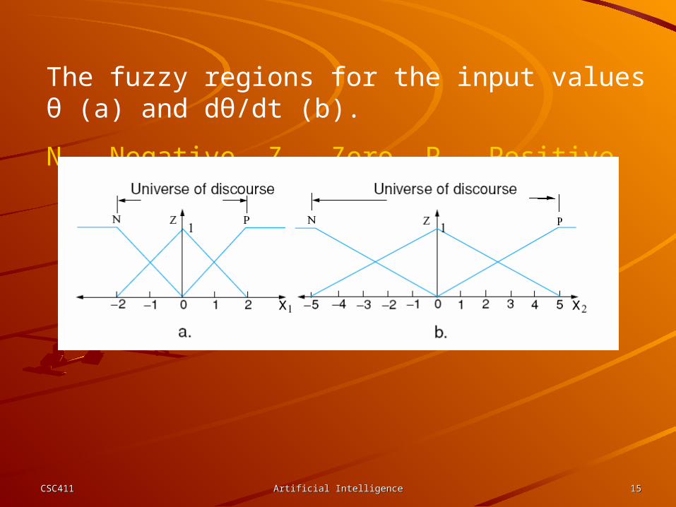
The fuzzy regions for the input values θ (a) and dθ/dt (b).
N – Negative, Z – Zero, P – Positive
CSC411CSC411 Artificial IntelligenceArtificial Intelligence 1616
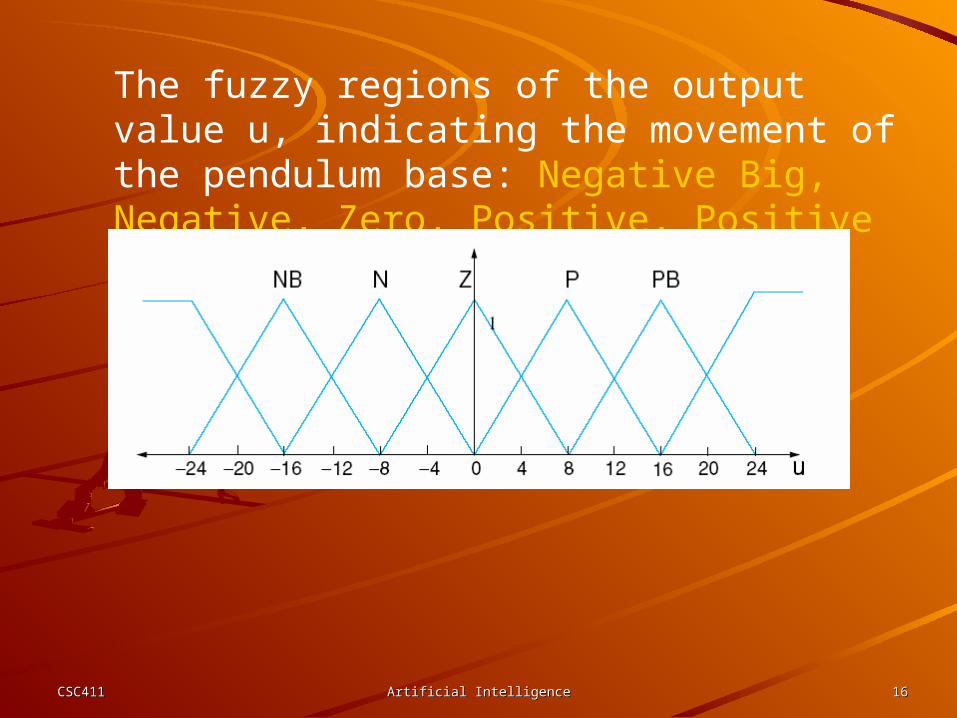
The fuzzy regions of the output value u, indicating the movement of the pendulum base: Negative Big, Negative, Zero, Positive, Positive Big.
CSC411CSC411 Artificial IntelligenceArtificial Intelligence 1717
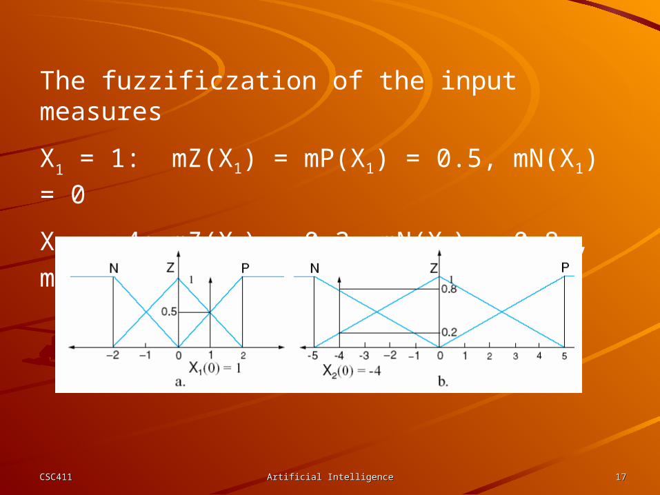
The fuzzificzation of the input measures
X1 = 1: mZ(X1) = mP(X1) = 0.5, mN(X1) = 0
X2 = -4: mZ(X2) = 0.2, mN(X2) = 0.8 , mP(X2) = 0
CSC411CSC411 Artificial IntelligenceArtificial Intelligence 1818
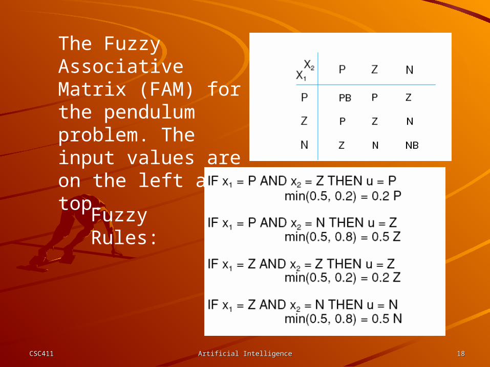
The Fuzzy Associative Matrix (FAM) for the pendulum problem. The input values are on the left and top.
Fuzzy Rules:

CSC411CSC411 Artificial IntelligenceArtificial Intelligence 1919
The fuzzy consequents (a) and their union (b). The centroid of the union (-2) is the crisp output.
CSC411CSC411 Artificial IntelligenceArtificial Intelligence 2020
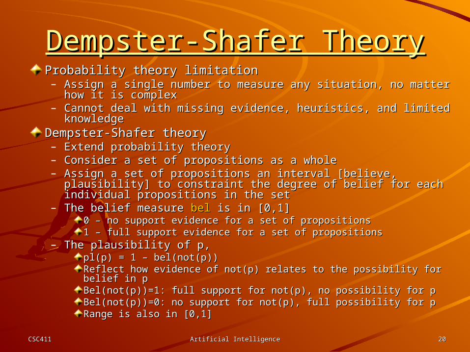
Dempster-Shafer TheoryDempster-Shafer TheoryProbability theory limitationProbability theory limitation– Assign a single number to measure any situation, no matter how Assign a single number to measure any situation, no matter how
it is complexit is complex– Cannot deal with missing evidence, heuristics, and limited Cannot deal with missing evidence, heuristics, and limited
knowledgeknowledgeDempster-Shafer theoryDempster-Shafer theory– Extend probability theoryExtend probability theory– Consider a set of propositions as a wholeConsider a set of propositions as a whole– Assign a set of propositions an interval [believe, plausibility] to Assign a set of propositions an interval [believe, plausibility] to
constraint the degree of belief for each individual propositions in constraint the degree of belief for each individual propositions in the setthe set
– The belief measure The belief measure belbel is in [0,1] is in [0,1]0 – no support evidence for a set of propositions0 – no support evidence for a set of propositions1 – full support evidence for a set of propositions1 – full support evidence for a set of propositions
– The plausibility of p, The plausibility of p, pl(p) = 1 – bel(not(p))pl(p) = 1 – bel(not(p))Reflect how evidence of not(p) relates to the possibility for belief in pReflect how evidence of not(p) relates to the possibility for belief in pBel(not(p))=1: full support for not(p), no possibility for pBel(not(p))=1: full support for not(p), no possibility for pBel(not(p))=0: no support for not(p), full possibility for pBel(not(p))=0: no support for not(p), full possibility for pRange is also in [0,1]Range is also in [0,1]
CSC411CSC411 Artificial IntelligenceArtificial Intelligence 2121
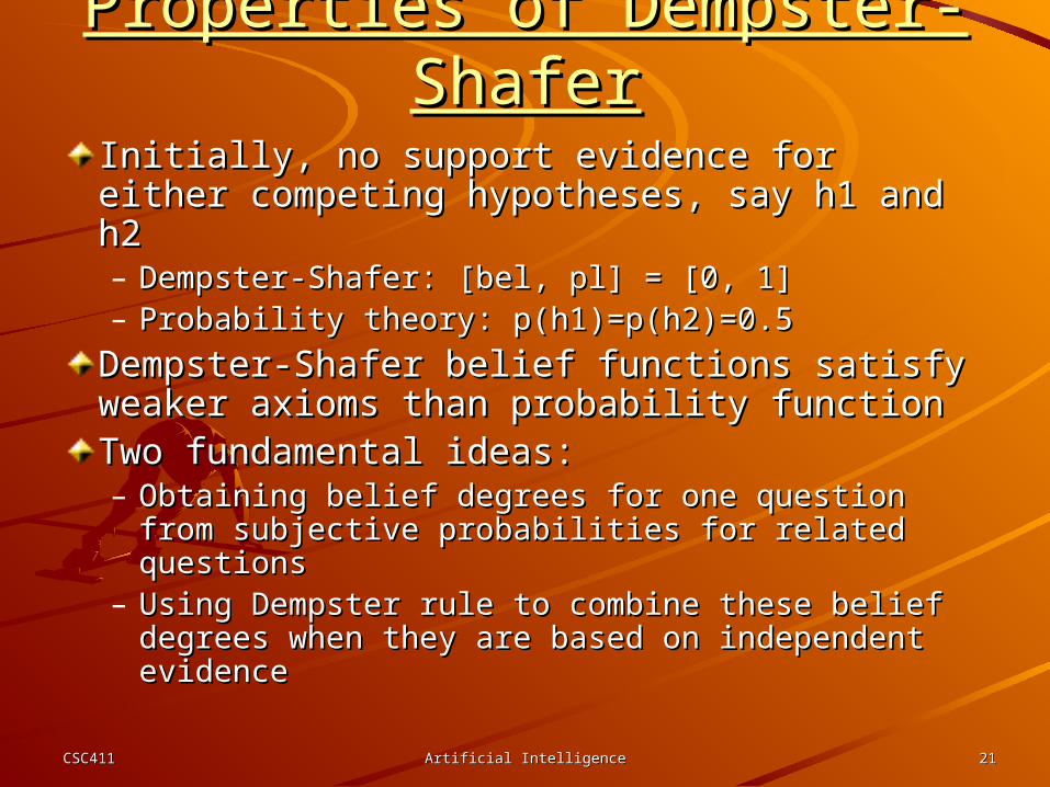
Properties of Dempster-ShaferProperties of Dempster-ShaferInitially, no support evidence for either Initially, no support evidence for either competing hypotheses, say h1 and h2competing hypotheses, say h1 and h2– Dempster-Shafer: [bel, pl] = [0, 1]Dempster-Shafer: [bel, pl] = [0, 1]– Probability theory: p(h1)=p(h2)=0.5Probability theory: p(h1)=p(h2)=0.5
Dempster-Shafer belief functions satisfy Dempster-Shafer belief functions satisfy weaker axioms than probability functionweaker axioms than probability functionTwo fundamental ideas:Two fundamental ideas:– Obtaining belief degrees for one question from Obtaining belief degrees for one question from
subjective probabilities for related questionssubjective probabilities for related questions– Using Dempster rule to combine these belief Using Dempster rule to combine these belief
degrees when they are based on independent degrees when they are based on independent evidence evidence
CSC411CSC411 Artificial IntelligenceArtificial Intelligence 2222
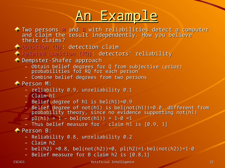
An ExampleAn ExampleTwo persons Two persons MM and and BB with reliabilities detect a computer and with reliabilities detect a computer and claim the result independently. How you believe their claims?claim the result independently. How you believe their claims?Question (Q)Question (Q): detection claim: detection claimRelated question (RQ)Related question (RQ): detectors’ reliability: detectors’ reliabilityDempster-Shafer approachDempster-Shafer approach– Obtain belief degrees for Q from subjective (prior) probabilities for RQ Obtain belief degrees for Q from subjective (prior) probabilities for RQ
for each personfor each person– Combine belief degrees from two personsCombine belief degrees from two persons
Person M: Person M: – reliability 0.9, unreliability 0.1reliability 0.9, unreliability 0.1– Claim h1 Claim h1 – Belief degree of h1 is bel(h1)=0.9Belief degree of h1 is bel(h1)=0.9– Belief degree of not(h1) is bel(not(h1))=0.0, different from probability Belief degree of not(h1) is bel(not(h1))=0.0, different from probability
theory, since no evidence supporting not(h1)theory, since no evidence supporting not(h1)– pl(h1) = 1 – bel(not(h1)) = 1-0 =1pl(h1) = 1 – bel(not(h1)) = 1-0 =1– Thus belief measure for Thus belief measure for MM claim h1 is [0.9, 1] claim h1 is [0.9, 1]
Person B:Person B:– Reliability 0.8, unreliability 0.2Reliability 0.8, unreliability 0.2– Claim h2Claim h2– bel(h2) =0.8, bel(not(h2))=0, pl(h2)=1-bel(not(h2))=1-0bel(h2) =0.8, bel(not(h2))=0, pl(h2)=1-bel(not(h2))=1-0– Belief measure for B claim h2 is [0.8,1] Belief measure for B claim h2 is [0.8,1]
CSC411CSC411 Artificial IntelligenceArtificial Intelligence 2323
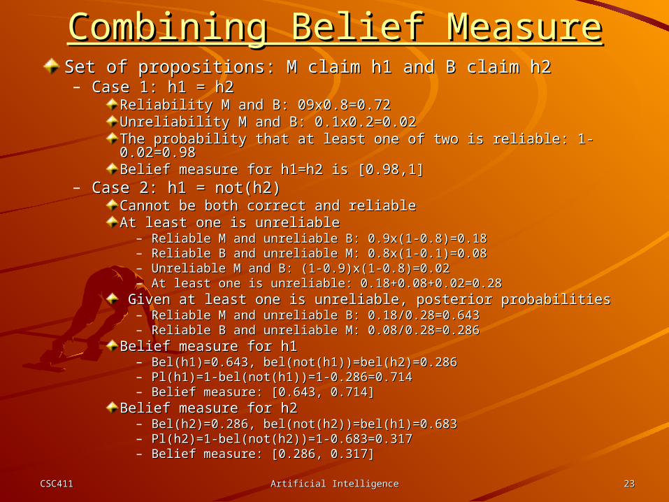
Combining Belief MeasureCombining Belief MeasureSet of propositions: M claim h1 and B claim h2Set of propositions: M claim h1 and B claim h2– Case 1: h1 = h2Case 1: h1 = h2
Reliability M and B: 09x0.8=0.72Reliability M and B: 09x0.8=0.72Unreliability M and B: 0.1x0.2=0.02Unreliability M and B: 0.1x0.2=0.02The probability that at least one of two is reliable: 1-0.02=0.98The probability that at least one of two is reliable: 1-0.02=0.98Belief measure for h1=h2 is [0.98,1]Belief measure for h1=h2 is [0.98,1]
– Case 2: h1 = not(h2)Case 2: h1 = not(h2)Cannot be both correct and reliableCannot be both correct and reliableAt least one is unreliableAt least one is unreliable
– Reliable M and unreliable B: 0.9x(1-0.8)=0.18Reliable M and unreliable B: 0.9x(1-0.8)=0.18– Reliable B and unreliable M: 0.8x(1-0.1)=0.08Reliable B and unreliable M: 0.8x(1-0.1)=0.08– Unreliable M and B: (1-0.9)x(1-0.8)=0.02Unreliable M and B: (1-0.9)x(1-0.8)=0.02– At least one is unreliable: 0.18+0.08+0.02=0.28At least one is unreliable: 0.18+0.08+0.02=0.28
Given at least one is unreliable, posterior probabilitiesGiven at least one is unreliable, posterior probabilities– Reliable M and unreliable B: 0.18/0.28=0.643Reliable M and unreliable B: 0.18/0.28=0.643– Reliable B and unreliable M: 0.08/0.28=0.286Reliable B and unreliable M: 0.08/0.28=0.286
Belief measure for h1Belief measure for h1– Bel(h1)=0.643, bel(not(h1))=bel(h2)=0.286Bel(h1)=0.643, bel(not(h1))=bel(h2)=0.286– Pl(h1)=1-bel(not(h1))=1-0.286=0.714Pl(h1)=1-bel(not(h1))=1-0.286=0.714– Belief measure: [0.643, 0.714]Belief measure: [0.643, 0.714]
Belief measure for h2Belief measure for h2– Bel(h2)=0.286, bel(not(h2))=bel(h1)=0.683Bel(h2)=0.286, bel(not(h2))=bel(h1)=0.683– Pl(h2)=1-bel(not(h2))=1-0.683=0.317Pl(h2)=1-bel(not(h2))=1-0.683=0.317– Belief measure: [0.286, 0.317]Belief measure: [0.286, 0.317]
CSC411CSC411 Artificial IntelligenceArtificial Intelligence 2424
Dempster’s RuleDempster’s RuleAssumption: Assumption:
– probable questions are independent a prioriprobable questions are independent a priori– As new evidence collected and conflicts, independency As new evidence collected and conflicts, independency
may disappearmay disappear
Two stepsTwo steps1.1. Sort the uncertainties into a priori independent pieces of Sort the uncertainties into a priori independent pieces of
evidenceevidence2.2. Carry out Dempster ruleCarry out Dempster rule
Consider the previous exampleConsider the previous example– After M and B claimed, a repair person is called to After M and B claimed, a repair person is called to
check the computer, and both M and B witnessed this.check the computer, and both M and B witnessed this.– Three independent items of evidence must be Three independent items of evidence must be
combinedcombined
Not all evidence is directly supportive of Not all evidence is directly supportive of individual elements of a set of hypotheses, but individual elements of a set of hypotheses, but often supports different subsets of hypotheses, often supports different subsets of hypotheses, in favor of some and against othersin favor of some and against others

CSC411CSC411 Artificial IntelligenceArtificial Intelligence 2525
General Dempster’s RuleGeneral Dempster’s RuleQ – an exhaustive set of mutually exclusive Q – an exhaustive set of mutually exclusive hypotheseshypotheses
Z – a subset of QZ – a subset of Q
M – probability density function to assign a M – probability density function to assign a belief measure to Zbelief measure to Z
MMnn(Z) – belief degree to Z, where n is the (Z) – belief degree to Z, where n is the number of sources of evidencesnumber of sources of evidences
CSC411CSC411 Artificial IntelligenceArtificial Intelligence 2626
Bayesian Belief NetworkBayesian Belief NetworkA computational model for reasoning to the best A computational model for reasoning to the best explanation of a data set in the uncertainty explanation of a data set in the uncertainty context context Motivation Motivation – Reduce the number of parameters of the full Bayesian Reduce the number of parameters of the full Bayesian
modelmodel– Show how the data can partition and focus reasoningShow how the data can partition and focus reasoning– Avoid use of a large joint probability table to compute Avoid use of a large joint probability table to compute
probabilities for all possible events combinationprobabilities for all possible events combination
AssumptionAssumption– Events are either conditionally independent or their Events are either conditionally independent or their
correlations are so small that they can be ignoredcorrelations are so small that they can be ignored
Directed Graphical ModelDirected Graphical Model– The events and (cause-effect) relationships form a The events and (cause-effect) relationships form a
directed graph, where events are vertices and directed graph, where events are vertices and relationships are linksrelationships are links

CSC411CSC411 Artificial IntelligenceArtificial Intelligence 2727
The Bayesian representation of the traffic problem with potential explanations.
The joint probability distribution for the traffic and construction variables
The Traffic Problem
Given bad traffic, what is the probability of road construction?
p(C|T)=p(C=t, T=t)/(p(C=t, T=t)+p(C=f, T=t))=.3/(.3+.1)=.75
CSC411CSC411 Artificial IntelligenceArtificial Intelligence 2828
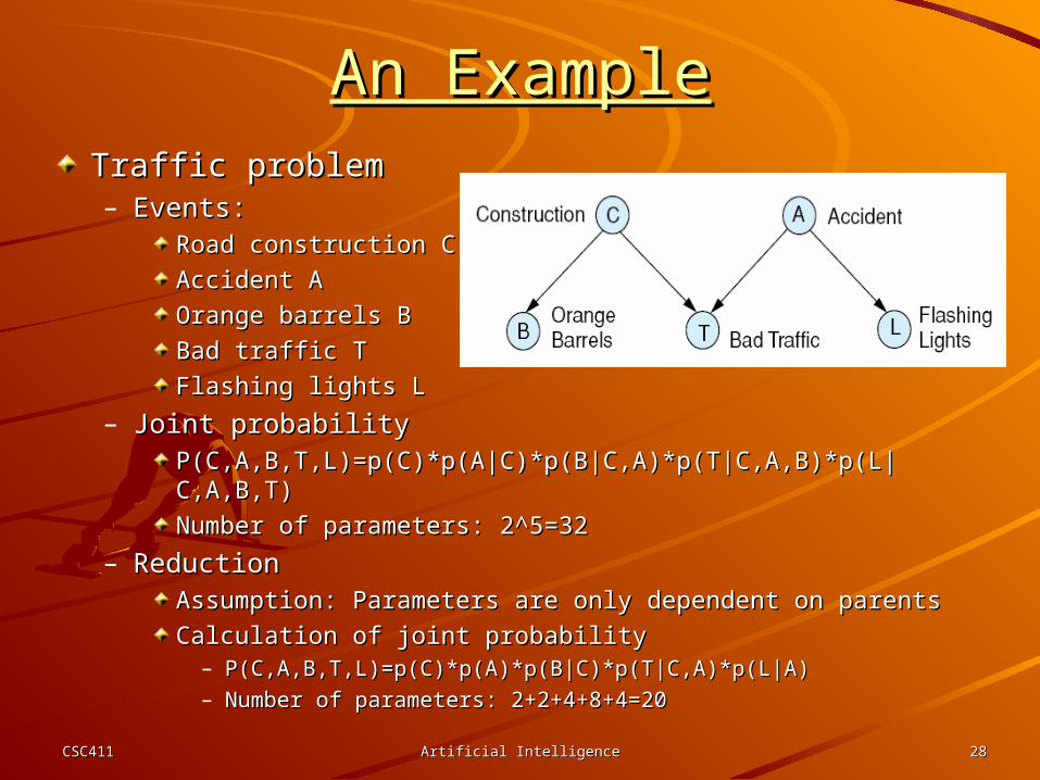
An ExampleAn ExampleTraffic problemTraffic problem– Events: Events:
Road construction CRoad construction C
Accident AAccident A
Orange barrels BOrange barrels B
Bad traffic TBad traffic T
Flashing lights LFlashing lights L
– Joint probabilityJoint probabilityP(C,A,B,T,L)=p(C)*p(A|C)*p(B|C,A)*p(T|C,A,B)*p(L|C,A,B,T)P(C,A,B,T,L)=p(C)*p(A|C)*p(B|C,A)*p(T|C,A,B)*p(L|C,A,B,T)
Number of parameters: 2^5=32Number of parameters: 2^5=32
– ReductionReductionAssumption: Parameters are only dependent on parentsAssumption: Parameters are only dependent on parents
Calculation of joint probabilityCalculation of joint probability– P(C,A,B,T,L)=p(C)*p(A)*p(B|C)*p(T|C,A)*p(L|A)P(C,A,B,T,L)=p(C)*p(A)*p(B|C)*p(T|C,A)*p(L|A)– Number of parameters: 2+2+4+8+4=20Number of parameters: 2+2+4+8+4=20
CSC411CSC411 Artificial IntelligenceArtificial Intelligence 2929
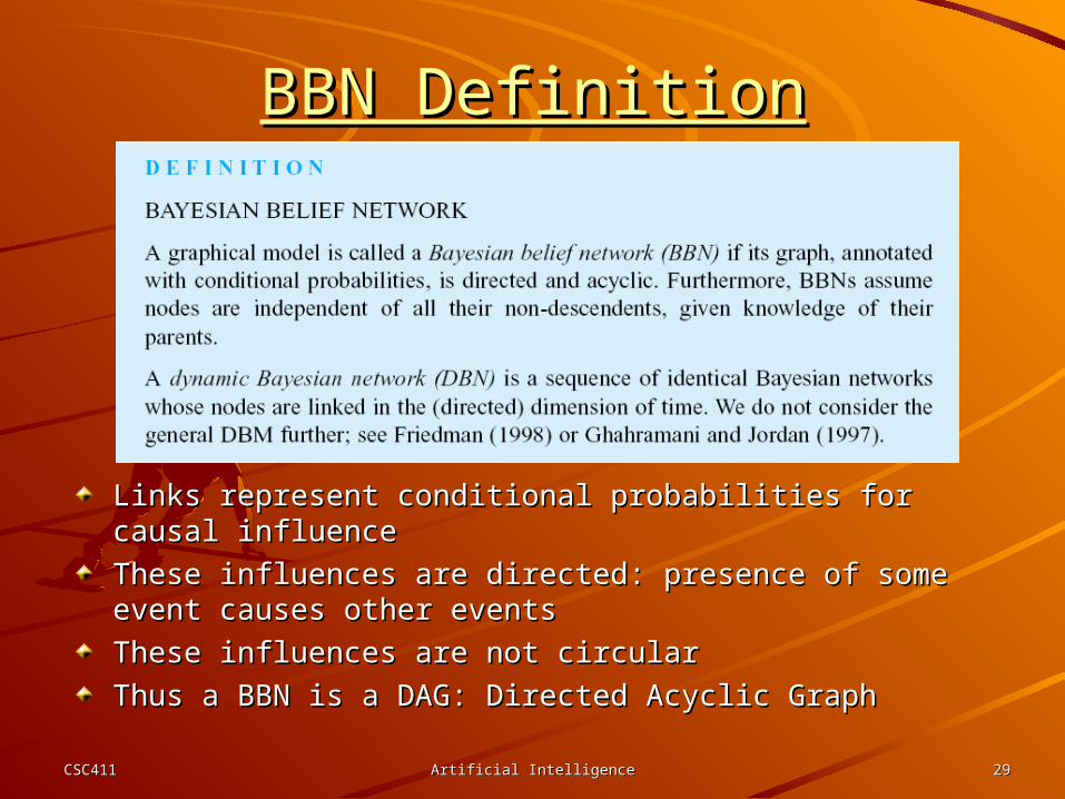
BBN DefinitionBBN Definition
Links represent conditional probabilities for causal influenceLinks represent conditional probabilities for causal influence
These influences are directed: presence of some event These influences are directed: presence of some event causes other eventscauses other events
These influences are not circularThese influences are not circular
Thus a BBN is a DAG: Directed Acyclic GraphThus a BBN is a DAG: Directed Acyclic Graph
CSC411CSC411 Artificial IntelligenceArtificial Intelligence 3030
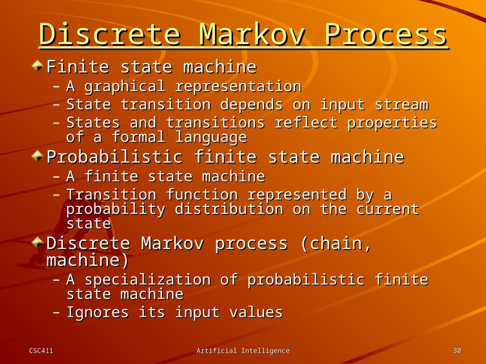
Discrete Markov ProcessDiscrete Markov ProcessFinite state machineFinite state machine– A graphical representationA graphical representation– State transition depends on input streamState transition depends on input stream– States and transitions reflect properties of a States and transitions reflect properties of a
formal languageformal languageProbabilistic finite state machineProbabilistic finite state machine– A finite state machineA finite state machine– Transition function represented by a probability Transition function represented by a probability
distribution on the current statedistribution on the current stateDiscrete Markov process (chain, machine) Discrete Markov process (chain, machine) – A specialization of probabilistic finite state A specialization of probabilistic finite state
machinemachine– Ignores its input values Ignores its input values
CSC411CSC411 Artificial IntelligenceArtificial Intelligence 3131
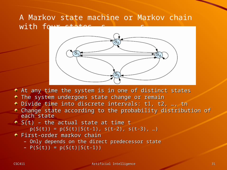
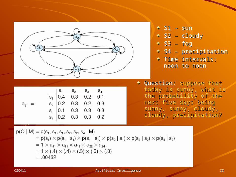
A Markov state machine or Markov chain with four states, s1, ..., s4
At any time the system is in one of distinct statesAt any time the system is in one of distinct statesThe system undergoes state change or remainThe system undergoes state change or remainDivide time into discrete intervals: t1, t2, …, tnDivide time into discrete intervals: t1, t2, …, tnChange state according to the probability distribution of each Change state according to the probability distribution of each statestateS(t) – the actual state at time tS(t) – the actual state at time t
p(S(t)) = p(S(t)|S(t-1), s(t-2), s(t-3), …)p(S(t)) = p(S(t)|S(t-1), s(t-2), s(t-3), …)First-order markov chainFirst-order markov chain– Only depends on the direct predecessor stateOnly depends on the direct predecessor state– P(S(t)) = p(S(t)|S(t-1))P(S(t)) = p(S(t)|S(t-1))
CSC411CSC411 Artificial IntelligenceArtificial Intelligence 3232
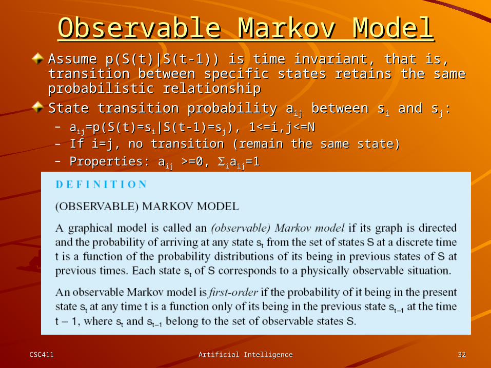
Observable Markov ModelObservable Markov ModelAssume p(S(t)|S(t-1)) is time invariant, that is, transition Assume p(S(t)|S(t-1)) is time invariant, that is, transition between specific states retains the same probabilistic between specific states retains the same probabilistic relationshiprelationship
State transition probability aState transition probability aijij between s between sii and s and sjj::– aaijij=p(S(t)=s=p(S(t)=sii|S(t-1)=s|S(t-1)=sjj), 1<=i,j<=N), 1<=i,j<=N– If i=j, no transition (remain the same state)If i=j, no transition (remain the same state)– Properties: aProperties: aijij >=0, >=0, iiaaijij=1=1
CSC411CSC411 Artificial IntelligenceArtificial Intelligence 3333
S1 – sunS1 – sunS2 – cloudyS2 – cloudyS3 – fogS3 – fogS4 – precipitationS4 – precipitationTime intervals: Time intervals: noon to noonnoon to noon
Question: Question: suppose that suppose that today is sunny, what is today is sunny, what is the probability of the the probability of the next five days being next five days being sunny, sunny, cloudy, sunny, sunny, cloudy, cloudy, precipitation?cloudy, precipitation?