credit scoring models for a tunisian microfinance institution ... · review of economics &...

Review of Economics & Finance Submitted on 04/07/2015

Article ID: 1923-7529-2016-01-61-18 Aïda Kammoun, and Imen Triki

~ 61 ~

Credit Scoring Models for a Tunisian Microfinance Institution: Comparison between Artificial Neural Network and Logistic Regression

Dr. Aïda Kammoun (Correspondence author)

Institut Supérieur d’Administration des Affaires de Sfax, Route El Matar Km 4.5, BP 1013, 3018

Sfax, TUNISIE

Tel: +0021-623-624-824/+0021-674-680-460, E-mail: [email protected]

Imen Triki

Institut Supérieur de Gestion de Tunis, 41, Avenue de la Liberté, Cité Bouchoucha, Le Bardo 2000,

Tunis, TUNISIE

Tel.: 0021-658-366-215, E-mail: [email protected]

Abstract: This paper compares, for a microfinance institution, the performance of two individual

classification models: Logistic Regression (Logit) and Multi-Layer Perceptron Neural Network

(MLP), to evaluate the credit risk problem and discriminate good creditors from bad ones. Credit

scoring systems are currently in common use by numerous financial institutions worldwide.

However, credit scoring using a non-parametric statistical technique with the microfinance industry,

is a relatively recent application. In Tunisia, no model which employs a non-parametric statistical

technique has yet, as far as we know, been published. This lack is surprising since the

implementation of credit scoring should contribute towards the efficiency of microfinance

institutions, thereby improving their competitiveness.

This paper builds a non-parametric credit scoring model based on the Multi-Layer perceptron

approach (MLP) and benchmarks its performance against Logistic Regression (LR) techniques.

Based on a sample of 300 borrowers from a Tunisian microfinance institution, the results reveal that

Logistic Regression outperforms neural network models.

Keywords: Micro finance institution; Credit scoring model; Multi-Layer perceptron; Logistic

Regression JEL Classifications: C14 ; C45 ; G21

1. Introduction

Credit risk analysis is an important topic in financial risk management. It gains new

importance following the recent financial crises and regulatory concerns of Basel II extended

by Basel III which have favored the emergence of the present climate of tight credit and interest on

the part of banks to minimize losses due to credit risk. The ability to discriminate good applicants

from bad ones is important for credit companies and commercial banks to succeed. In fact, how a

bank manages its credit risk is crucial to its performance over time.

Different modeling approaches have been developed for the assessment of credit risk rating,

trying to determine the best credit approval programs. These credit scoring models have attracted

serious attention over the last decade. According to Anderson (2007), credit scoring can be defined

as “the use of statistical models to transform relevant data into numerical measures that guide credit

decisions”.

ISSNs: 1923-7529; 1923-8401 © 2016 Academic Research Centre of Canada

~ 62 ~

Classical statistical methods that are used to develop credit scoring models are Linear

Discriminant Analysis (LDA) and linear Regression (Logit, Probit, Tobit). There are also more

sophisticated methods known as artificial intelligence, such as fuzzy systems, genetic algorithms

and neural networks. Among these, the most commonly used as an alternative to Logistic

Regression is neural networks due to the possible complex, nonlinear relationship between

variables.

Nowadays, most researchers are likely to want to compare statistical models, since each model

has advantages and drawbacks and since the computational time is no longer a problem. The results

of these studies are controversial. Some authors find that Neural Networks are more accurate than

Logistic Regression (West 2000, Blanco et al. 2013). Other papers find that parametric approaches

give better results such as Komorád (2009), who concluded the primacy of the classical method

"LR" compared to ANNs, particularly Multi-Layer Perceptron (MLP) architecture and Radial Basis

Function (RBF).

Credit scoring systems are currently in common use by numerous financial institutions

worldwide. However, credit scoring using a non-parametric statistical technique with the

microfinance industry is a relatively recent application. In Tunisia, no model employing a non-

parametric statistical technique has yet, as far as we know, been published. This lack is surprising

since the implementation of credit scoring should contribute towards the efficiency of microfinance

institutions, thereby improving their competitiveness.


approach (MLP) and benchmarks its performance against Logistic Regression (LR) techniques. It is

organized as follows: the following section will be devoted to briefly explain the credit risk puzzle

and to present credit scoring models, namely Logistic Regression and Artificial Neural Networks.

Section3 describes the sample and variables measurement first and then provides the process and

implementation of the Credit Scoring Methods for credit risk evaluation, using two different

models: Logistic Regression and Multi-Layer Perceptron neural networks. The fourth section will

present the results of the credit scoring models separately then in a comparative approach, by

applying the classification/evaluation criteria.

2. Credit Risk Puzzle and Credit Scoring Models

Historically, the credit risk is one of the traditional and important risks in the financial market.

Known as counterparty risk, it can be simply defined as the potential that a borrower or

counterparty doesn’t respect its obligations under agreed terms (Robert A. Klein, 1992). According

to Duffie and Singleton (2003), “credit risk is the risk of default or of reductions in market value

caused by changes in the credit quality of issuers or counterparties”. It is the potential for loss due

to failure of a borrower to meet its contractual obligation to repay a debt in accordance with the

agreed terms. In the banking sector, the credit risk tends to increasingly evolve. That’s why the

apprehension of risk by the bankers is an important issue and the capacity to discriminate good

customers from bad ones is paramount. The improvement of a consistent distinction between good

and bad payers allows the bank to reject riskier loans and to adjust the terms of the granted credits

given default risk.

Credit risk problem is a real puzzle for theorists and researchers because it comes from

asymmetric information, which causes the moral hazard and adverse selection problems. “All

contracts and transactions are based on information (Casu, Girardone, Molyneux, 2006). In

financial intermediation certain problems can occur: not all participants have the same information;

all participants are not perfectly informed; part of the transaction can hold “inside” information,

Review of Economics & Finance, Volume 6, Issue 1

~ 63 ~

which is not available to both parties. The information asymmetry (or informational asymmetry)

can generate problems regarding the adverse selection and the moral hazard which can make the

signing of financial agreements difficult decreasing the interest of participants and leading to the

inefficiency of the financial intermediation” (Andrieş, 2008). In adverse selection models, one party

lacks information while contract to the transaction. Moral hazard, qualified as a model with ex-post

asymmetric information, refers to a situation in which the asymmetric information problem is

created after the transaction occurs. It’s also called ongoing asymmetric information. In other terms,

moral hazard comes from the inability of lenders to observe the actions of the borrower that affect

the probability of repayment.

Facing these information asymmetries and the risks that they carry, a question arises: what

mechanisms can be implemented by the banker to overcome these problems?

In order to avoid adverse selection and moral hazard, the bank may proceed to a credit

rationing from a certain level of credit corresponding to any rate, where it maximizes its

performance. Credit rationing is a partial or total solution: it’s better not to grant a credit when we

anticipate a high risk rather than lend at high rate and thus increase disincentives effects to

repayment (Rougès, 2003). Besides, the guarantees can play an important role in the failure

analysis. Even if the lender knows the quality of the borrower, guarantees help to reduce or

eliminate the moral hazard and adverse selection problems once the credit is granted (Diallo, 2006).

Furthermore, another way to reduce asymmetric information is to use Credit Scoring which is based

on borrower characteristics to distinguish between good and bad customers. Matoussi and

Abdelmoula (2010) distinguish 4 borrower characteristics: borrower size, the quality of bank-firm

relationship (fidelity), time as a factor for clarification of the bank-borrower relationship, and finally

personal characteristics: (age, sex, profession ...).

Credit scoring systems are currently in common use by numerous Micro finance Institutions.

In fact, one way for the IMFs to become more efficient is the implementation of automatic credit

scoring systems to evaluate their credit applicants since credit scoring reduces the cost of credit

analysis, enables faster credit decisions, reduces the losses, and also results in the closer monitoring

of existing accounts and the prioritization of repayment collection (Blanco et al. (2013)).

Nevertheless, the development of credit scoring models in the microfinance sector is based on

traditional parametric statistical techniques, mainly linear discriminated analysis (LDA) and logistic

regression (LR), despite the overwhelming evidence found in numerous studies which indicates that

the nonparametric methodologies usually outperform these classic statistical models (for example,

see Lee & Chen, 2005; West, 2000). As far as we know, in the existing literature, only one credit

scoring model designed for the microfinance industry applies a non-parametric methodology, and

therefore, the microfinance industry has not benefited from the advantages of non-parametric

techniques to improve the performance of credit scoring models yet.

2.1 Logistic Regression (LR) approach

Logistic Regression is one of the most commonly used techniques in prediction and

classification problems. It’s a special case of the Generalized Linear Model (GLM), which is a

flexible generalization of Ordinary Least Squares (OLS) regression (Komorád, 2009).

Logistic Regression is a parametric probabilistic approach which consists in producing a

model to predict the values taken by a categorical dependent variable, usually binary, from a series

of independent variables, which can be discrete or continuous. “Logistic regression is one of the

most widely used statistical techniques in the field. What distinguishes a logistic regression model

from a linear regression model is that the outcome variable in logistic regression is dichotomous (a

0/1 outcome). This difference between logistic and linear regression is reflected both in the choice

of a parametric model and in the assumptions. Once this difference is accounted for, the methods


~ 64 ~

employed in an analysis using logistic regression follow the same general principles used in linear

regression (Hosmer & Lemeshow, 1989). The simple logistic regression model can easily be

extended to two or more independent variables. Of course, the more variables, the harder it is to get

multiple observations at all levels of all variables. Therefore, most logistic regressions with more

than one independent variable are done using the maximum likelihood method (Freund & William,

1998). On theoretical grounds it might be supposed that logistic regression is a more proper

statistical instrument than linear regression, given that the two classes “good” credit and “bad”

credit have been described” (Abdou & Pointon, 2011).

Boisselier and Dufour (2003) present the specificities of the LR model as follows: “Logistic

Regression is a technique used to analyze the determinants of a variable, which is the dependent

variable. This variable is binary and so takes only two values. The explanatory variables can be

continuous or discrete. Indeed, the methodology of Logistic Regression can be extended to the case

of more than two values for a dependent variable”.

The objective of the LR model is not to predict a numerical value of the dependent variable,

but to predict the probability that this individual has the characteristic associated with a code of the

dependent variable knowing the values taken by the independent variables of a given individual.

The major advantage of the Logistic Regression is to quantify the strength of association

between the dependent variable and each independent variable, considering the effect of other

predictors in the model. This technique doesn’t require constraints on the normality or

homoscedasticity of the variables distributions. In fact, according to Elizabeth Mays (2001), the

advantages of Logistic Regression are that it does not require any assumptions about population

distribution such as normality and equal variance and covariance’s. Besides, Logistic regression

was superior to linear discriminant function in performance. The major disadvantage is that small

samples may cause unstable estimation.

2.2 Artificial Neural Network (ANN) approach

Artificial Neural Networks (ANNs) are tools aimed to reproduce human reasoning and are

among the latest tools discussed by researchers in decision (Rougès, 2003).

Jeatrakul and Wong (2009) suggest the following definition: "Artificial Neural Network is a

technique based on the neural structure of the brain that reproduces the learning capability from

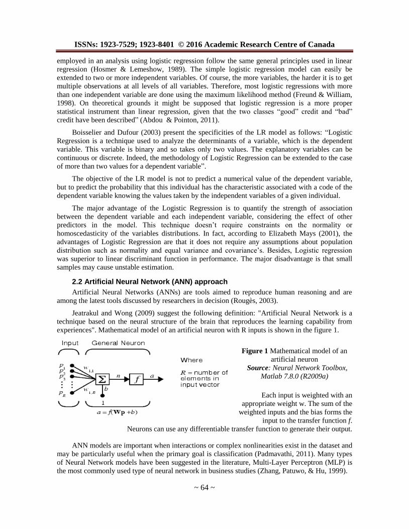
experiences". Mathematical model of an artificial neuron with R inputs is shown in the figure 1.

Figure 1 Mathematical model of an

artificial neuron

Source: Neural Network Toolbox,

Matlab 7.8.0 (R2009a)

Each input is weighted with an

appropriate weight w. The sum of the

weighted inputs and the bias forms the

input to the transfer function f.

Neurons can use any differentiable transfer function to generate their output.

ANN models are important when interactions or complex nonlinearities exist in the dataset and

may be particularly useful when the primary goal is classification (Padmavathi, 2011). Many types

of Neural Network models have been suggested in the literature, Multi-Layer Perceptron (MLP) is

the most commonly used type of neural network in business studies (Zhang, Patuwo, & Hu, 1999).


~ 65 ~

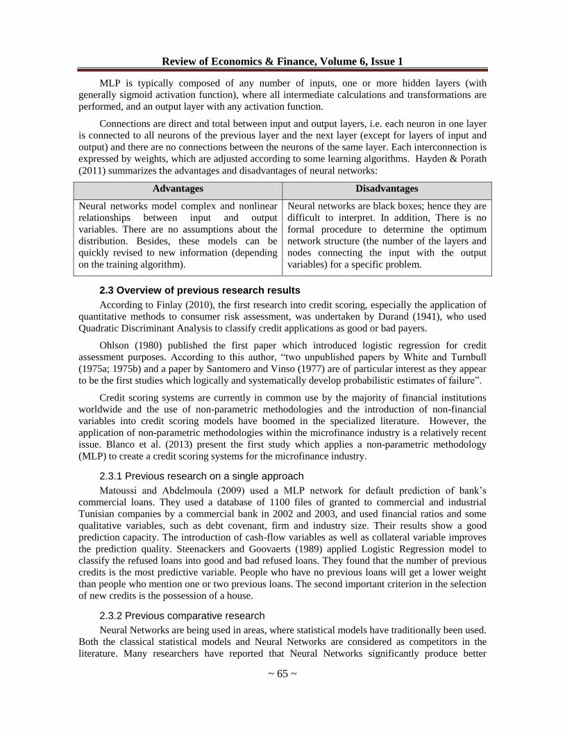
MLP is typically composed of any number of inputs, one or more hidden layers (with

generally sigmoid activation function), where all intermediate calculations and transformations are

performed, and an output layer with any activation function.

Connections are direct and total between input and output layers, i.e. each neuron in one layer

is connected to all neurons of the previous layer and the next layer (except for layers of input and

output) and there are no connections between the neurons of the same layer. Each interconnection is

expressed by weights, which are adjusted according to some learning algorithms. Hayden & Porath

(2011) summarizes the advantages and disadvantages of neural networks:

Advantages Disadvantages

Neural networks model complex and nonlinear

relationships between input and output

variables. There are no assumptions about the

distribution. Besides, these models can be

quickly revised to new information (depending

on the training algorithm).

Neural networks are black boxes; hence they are

difficult to interpret. In addition, There is no

formal procedure to determine the optimum

network structure (the number of the layers and

nodes connecting the input with the output

variables) for a specific problem.

2.3 Overview of previous research results

According to Finlay (2010), the first research into credit scoring, especially the application of

quantitative methods to consumer risk assessment, was undertaken by Durand (1941), who used

Quadratic Discriminant Analysis to classify credit applications as good or bad payers.

Ohlson (1980) published the first paper which introduced logistic regression for credit

assessment purposes. According to this author, “two unpublished papers by White and Turnbull

(1975a; 1975b) and a paper by Santomero and Vinso (1977) are of particular interest as they appear

to be the first studies which logically and systematically develop probabilistic estimates of failure”.

Credit scoring systems are currently in common use by the majority of financial institutions

worldwide and the use of non-parametric methodologies and the introduction of non-financial

variables into credit scoring models have boomed in the specialized literature. However, the

application of non-parametric methodologies within the microfinance industry is a relatively recent

issue. Blanco et al. (2013) present the first study which applies a non-parametric methodology

(MLP) to create a credit scoring systems for the microfinance industry.

2.3.1 Previous research on a single approach

Matoussi and Abdelmoula (2009) used a MLP network for default prediction of bank’s

commercial loans. They used a database of 1100 files of granted to commercial and industrial

Tunisian companies by a commercial bank in 2002 and 2003, and used financial ratios and some

qualitative variables, such as debt covenant, firm and industry size. Their results show a good

prediction capacity. The introduction of cash-flow variables as well as collateral variable improves

the prediction quality. Steenackers and Goovaerts (1989) applied Logistic Regression model to

classify the refused loans into good and bad refused loans. They found that the number of previous

credits is the most predictive variable. People who have no previous loans will get a lower weight

than people who mention one or two previous loans. The second important criterion in the selection

of new credits is the possession of a house.

2.3.2 Previous comparative research

Neural Networks are being used in areas, where statistical models have traditionally been used.

Both the classical statistical models and Neural Networks are considered as competitors in the

literature. Many researchers have reported that Neural Networks significantly produce better


~ 66 ~

classification/ prediction accuracy than classical statistical models (Discriminant Analysis and

Logistic Regression). One of the first researches of NNs in credit scoring applications was

conducted by Altman et al. (1994), who compared Linear Discriminant Analysis (LDA) and

Logistic regression (LR) with Neural Networks (NNs) in distress classification and prediction

problems. He showed that LDA was the best approach in performance. Diallo (2006) compared two

traditional approaches, Discriminant Analysis (DA) and Logistic Regression (LR), to predict the

probability of default of new credit applicants. Jeatrakul and Wong (2009) presented a comparison

of five different types of Neural Networks (NNs) for binary classification and prediction problem.

The main objective of the research of Muller, Steyn-Bruwer and Hamman (2009) was to test

whether some modeling techniques would in fact provide better prediction accuracies than other

modeling techniques. The different modeling techniques considered were: Multiple discriminant

analysis (MDA), Recursive partitioning (RP), Logit analysis (LA) and Neural networks (NN). It

was found that the LA and NN techniques provide the best overall predictive accuracy. Matoussi &

Abdelmoula (2010) show the superiority of ANNs compared with traditional methods in financial

distress of borrowing firms. They concluded that the implementation of ANNs has increased by

18% of the profits of the user company compared to performance of conventional systems generally

based on Discriminant Analysis. Bensic et al. (2005) aimed to extract important features for the

credit scoring model for small business, as well as to compare the performance of Logistic

Regression, Classification and Regression Trees (CART) decision tree and Neural Network models

on a Croatian dataset. Komroàd (2009) compared between LR model, MLP and RBF network using

a data set from a French bank. The results indicate that the methods used give very similar results,

however, the traditional Logit model seems to outperform the other techniques. Padmavathi (2011)

compared the performance of the RBF network with the MLP network and the classical LR model.

He concluded that ANN models had a better predictive power compared to LR model. Escaño et al.

(2006) have considered the usefulness of classical models, like LR models versus new approaches,

like Neural Networks. By comparing these models, they concluded that none of these models have

indicated better results.

Some researchers are specialized in the bankruptcy prediction field and have illustrated the

link between traditional Bayesian classification theory, namely Logistic Regression and Neural

Networks. Zhang et al. (1999), based on a sample of 220 firms, found that NNs are significantly

better than LR models in prediction as well as classification rate estimation. Tseng and Hu (2010)

have compared the accuracy of four forecasting techniques (logit model, quadratic interval logit

model, Back-Propagation MLP and RBF) in predicting the corporate distress of UK companies. In

general, ANN are promising alternative models that should be given much consideration when

solving real problems like bankruptcy prediction (Zhang et al., 1999). The MLP network is the most

widely used architecture of ANNs, which requires a larger training data than LR model in order to

reach a given level of accuracy and / or stability.

As a conclusion, it appears that the results of these studies are controversial. Some authors find

that Neural Networks are more accurate than Logistic Regression. Other papers find that parametric

approaches give better results.

3. Data, Variables, Parametric and Non-parametric Approaches

3.1 The data set

Our credit dataset contains 300 individual borrowers of a Tunisian Micro Finance Institution

(IMF) named “La Banque Tunisienne de Solidarité (BTS)”. The credits granted by this IMF are

used to finance the acquisition of equipment and small machinery (income generating loans). It also

provides consumer loans: non- revenue generating, and the amount of these loans is very small (less


~ 67 ~

than 1000 dinars). This study focuses only on income generating loans. Data are from the database

of the IMF relating to its customers (documentary research). A random selection of client files was

made. The sample consists of 300 credit files observed over a period from 2002 to 2009. BTS does

not provide simultaneous multiple loans to the same customer (except at the end of the first credit).

Thus the credit to the customer may not be the first; it can be a second after repaying the first one.

The loan repayment is always monthly. A client is at risk of default if one or more maturities

have not been paid. The dependent variable to explain is then the delay in payment which is

measured by a binary variable that takes 0 if the customer has no default and 1 in the opposite case,

which is if the customer has a late payment of one month, or more.

We collect customer information’s related to personal characteristics (age, matrimonial

status, gender and education), credit characteristics (credit amount, maturity, credit number, grace

period and time lag between the demand for credit and the release of credit) and project

characteristics (sector, activity and geographical location).

Our main objective is to develop credit analysis models which can distinguish good borrowers

from bad ones. Our sample consists of 300 credit files; only 29.33% do not present a risk of default

of payment, while 70.67% have at least one monthly payment due and unpaid.

3.2 Input variables

Table 1 presents input variables: type (categorical or numerical), notation and value.

In our empirical model, the sex of the borrower “Gender” is a dummy variable that takes 0 for

a man and 1 otherwise. “AGE” is the age of the borrower, measured in number of years. The

“Maturity” variable represents the repayment period specified in the contract in years. It’s a

numerical variable measured in years. For our sample, maturity takes values between 0.9151 (or 11

months) and 15.84 (15 years and 10 months). The expected effect of the variable “AGE” on the

repayment rate is positive. Many authors argue that financial institutions have a preference for

youth entrepreneurs. This criterion indicates an effect on the health of the contractor, his

commitment, his ability to take the risk, etc. By cons, it is expected that the effect of variables

(Maturity and Cmtbts) on the repayment rate is negative. However, as reported by Godquin (2004),

the effect of two variables (AGE, Maturity) is not always known. “Education” is a variable

measuring the level of education of the borrower that takes 0 if the borrower has not reached

university and 1 otherwise. The more the individual is educated, the more likely to meet his

commitment (positive sign). Some authors (Boissin, Castagnos and Deschamps, 2003; Bachelet et

al., 2004; Lasch, Drillon and Merdji, 2004) confirm that entrepreneur graduates have more specific

skills and knowledge for the creation and innovation. So they have high chances of success of their

projects and a lower default risk. The effect of marital status was measured by introducing three

dummy variables relating respectively to “divorced”, “widowed”, “single” and “married” status.

The single borrower has less financial commitments, so he tends to meet his commitment. On the

other hand, family stability is a factor promoting compliance.

“Nbrcred” is a variable measuring the experience of the IMF with the borrower. It is measured

by the number of loans granted to the client.

Repayment capacity can depend on the industry in which the borrower operates as well as the

project activity. Two categorical variables were thus included in the model and which relate

respectively to the sector and the project activity. Besides, since the BTS may allow for a grace

period, a numerical variable "Grace" was created, it is measured in years. Finally, a variable

measuring the waiting time before obtaining a credit is introduced, it takes values between 0.104 (or

38 days) and 2.26 (or 27 months that is 2 years and 3 months).


~ 68 ~

Table 1 Input variables

Customer

information Variables Notations Class Value

Personal

characteristics

Gender Gender Categorial 0 : male

1 : female

Education Educ Categorial 0 : not graduate from university

1 : graduate from University

Matrimonial status Matrim Categorial 0 : Single

1 : Married

2 : Divorced

3 : Widower

Age Age Numerical [27.5-66]

Project

characteristics

Sector Sect Categorial 0: industry

1: service

2: agriculture

3: commerce

4: tourism

Activity Act Categorial 0: service

1: small business

2: agriculture

3: handicrafts

Geographical

location

Geog Categorial 0 : Sfax (city center)

1 : Kerkennah (an Island)

2 : urban area away from the city

center between 4 and 12 km

3: urban area away from the city

center more than 12 km

Credit

characteristics

Credit amount Cmtbts Numerical [883.200-40800.000]

Maturity Maturity Numerical [0.9151-15.8493]

Credit number Nbcred Numerical [1-3]

Grace period Grace Numerical [0-0.69]

Waiting time DistGet Numerical [0.104-2.26]

3.3 Descriptive statistics

Our sample is composed of 300 credit files, with the following personal characteristics: the

average age is 47 years with a minimum of 27 years and a maximum of 66 years. The majority are

married (83.33%), there are 13.33% singles, 2.33% divorced and 0.67% widowers. 82.33% of the

sample is men against 17.67% women. Finally, the majority of the sample is literate but did not

graduate from university (91%) against 9% of the sample have a university degree.

Sector: we distinguish five sectors; 34% work in industry, 25% in service, 22.33% in agriculture,

13% in commerce and 5.67% in tourism.

Activity Another classification can be proposed: 36.67% in the service sector, 37.33% in small

business, 22.33% in agriculture and 3.67% in handicrafts.

Geographical region: the sites of the sample are distributed in four regions; there are 29% who live

in Sfax (city center), 2.33% in Kerkennah, 31.33% in Suburbs1 (urban area away from the

city center between 4-12 km) and 37.33% in Suburbs2 (urban area away from the city center

more than 12 km).


~ 69 ~

Number of credits received: the majority of borrowers in our sample have received one credit

(88.67%), only one borrower (0.67%) has received 3 credits and (10.67%) of sample has

received 2 credits.

Waiting time: is the delay between the deposit of credit record by the borrower and obtaining the

agreement by the bank. It is the time lag between the demand for credit and the release of

credit. The loans are approved in average after 188 days (about 6months) with a minimum of

38 days and a maximum of 825 days (about 27 months).

Credit amount: the credit amount is between a minimum of about 883 TND and a maximum of

40800 TND. The average credit amount is 5 758,626TND.

Grace period: is a period of time during which a payment can be made or late performance can

occur without incurring any late penalties, fees or interest. The average of grace period is

approximately 107 days (about three months and half) with a minimum of 0 days and a

maximum of 252 days (8 months).

Credit maturity: the average maturity is about 6 years with a minimum of approximately 11

months (334 days) and a maximum of approximately 16 years.

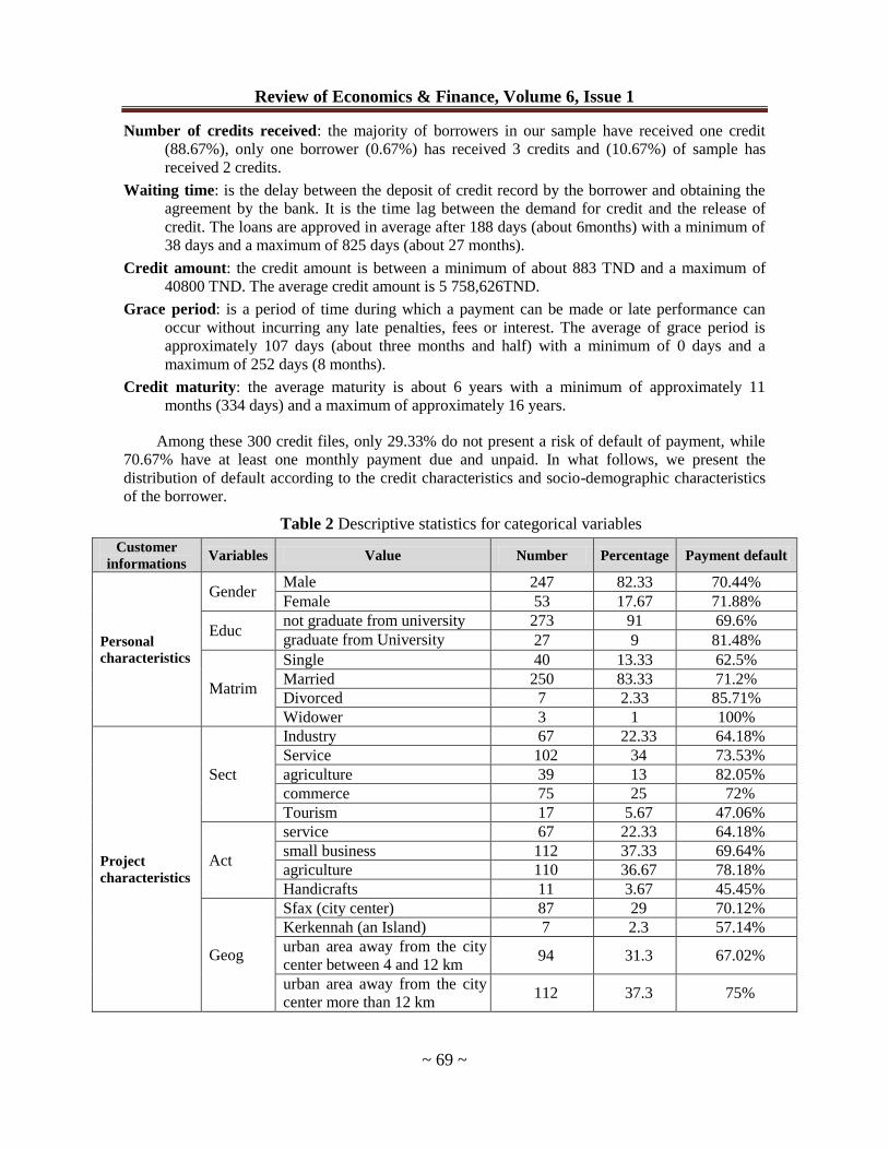
Among these 300 credit files, only 29.33% do not present a risk of default of payment, while

70.67% have at least one monthly payment due and unpaid. In what follows, we present the

distribution of default according to the credit characteristics and socio-demographic characteristics

of the borrower.

Table 2 Descriptive statistics for categorical variables

Customer

informations Variables Value Number Percentage Payment default

Personal

characteristics

Gender Male 247 82.33 70.44%

Female 53 17.67 71.88%

Educ not graduate from university 273 91 69.6%

graduate from University 27 9 81.48%

Matrim

Single 40 13.33 62.5%

Married 250 83.33 71.2%

Divorced 7 2.33 85.71%

Widower 3 1 100%

Project

characteristics

Sect

Industry 67 22.33 64.18%

Service 102 34 73.53%

agriculture 39 13 82.05%

commerce 75 25 72%

Tourism 17 5.67 47.06%

Act

service 67 22.33 64.18%

small business 112 37.33 69.64%

agriculture 110 36.67 78.18%

Handicrafts 11 3.67 45.45%

Geog

Sfax (city center) 87 29 70.12%

Kerkennah (an Island) 7 2.3 57.14%

urban area away from the city

center between 4 and 12 km 94 31.3 67.02%

urban area away from the city

center more than 12 km 112 37.3 75%


~ 70 ~

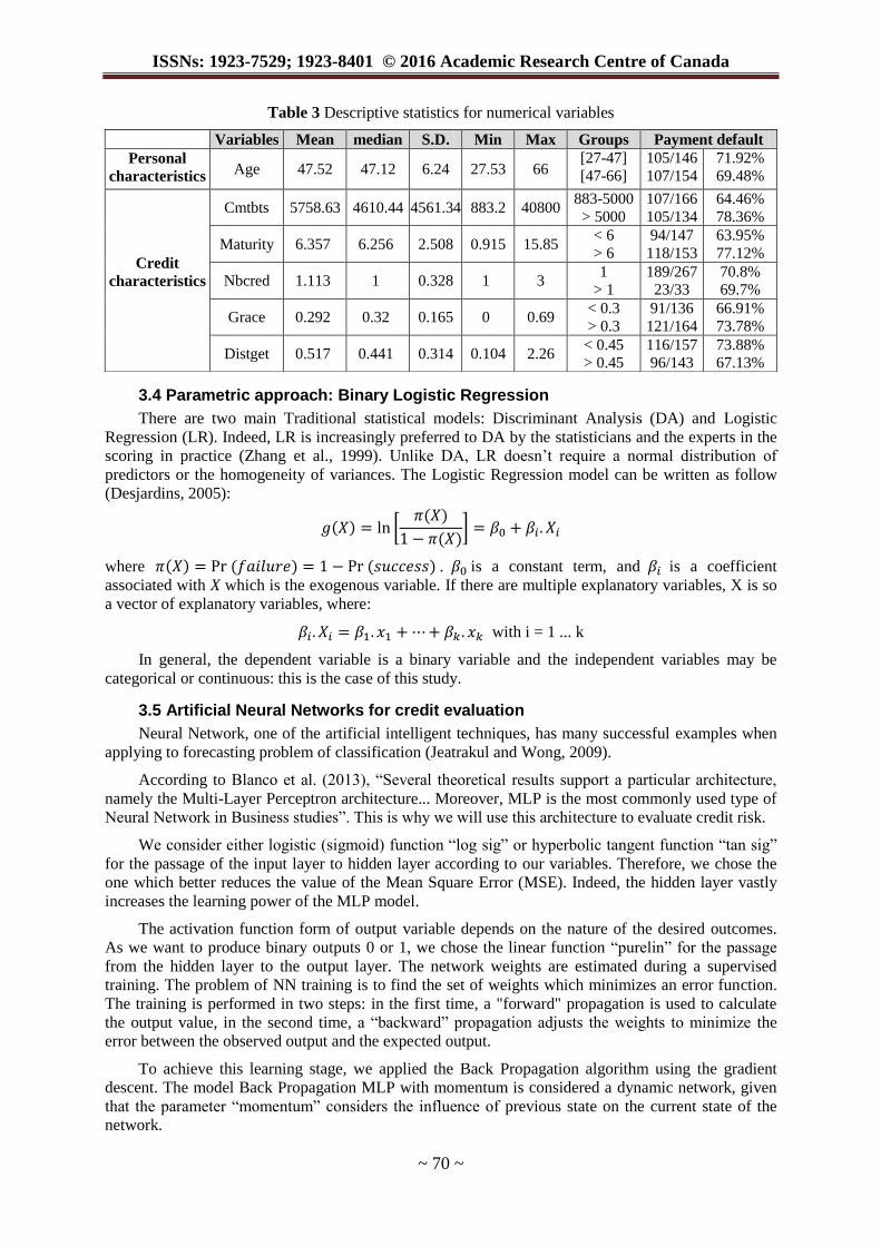
Table 3 Descriptive statistics for numerical variables

3.4 Parametric approach: Binary Logistic Regression

There are two main Traditional statistical models: Discriminant Analysis (DA) and Logistic

Regression (LR). Indeed, LR is increasingly preferred to DA by the statisticians and the experts in the

scoring in practice (Zhang et al., 1999). Unlike DA, LR doesn’t require a normal distribution of

predictors or the homogeneity of variances. The Logistic Regression model can be written as follow

(Desjardins, 2005):

where . is a constant term, and is a coefficient

associated with X which is the exogenous variable. If there are multiple explanatory variables, X is so

a vector of explanatory variables, where:

with i = 1 ... k

In general, the dependent variable is a binary variable and the independent variables may be

categorical or continuous: this is the case of this study.

3.5 Artificial Neural Networks for credit evaluation

Neural Network, one of the artificial intelligent techniques, has many successful examples when

applying to forecasting problem of classification (Jeatrakul and Wong, 2009).

According to Blanco et al. (2013), “Several theoretical results support a particular architecture,

namely the Multi-Layer Perceptron architecture... Moreover, MLP is the most commonly used type of

Neural Network in Business studies”. This is why we will use this architecture to evaluate credit risk.

We consider either logistic (sigmoid) function “log sig” or hyperbolic tangent function “tan sig”

for the passage of the input layer to hidden layer according to our variables. Therefore, we chose the

one which better reduces the value of the Mean Square Error (MSE). Indeed, the hidden layer vastly

increases the learning power of the MLP model.

The activation function form of output variable depends on the nature of the desired outcomes.

As we want to produce binary outputs 0 or 1, we chose the linear function “purelin” for the passage

from the hidden layer to the output layer. The network weights are estimated during a supervised

training. The problem of NN training is to find the set of weights which minimizes an error function.

The training is performed in two steps: in the first time, a "forward" propagation is used to calculate

the output value, in the second time, a “backward” propagation adjusts the weights to minimize the

error between the observed output and the expected output.

To achieve this learning stage, we applied the Back Propagation algorithm using the gradient

descent. The model Back Propagation MLP with momentum is considered a dynamic network, given

that the parameter “momentum” considers the influence of previous state on the current state of the

network.

Variables Mean median S.D. Min Max Groups Payment default

Personal

characteristics Age 47.52 47.12 6.24 27.53 66

[27-47]

[47-66]

105/146

107/154

71.92%

69.48%

Credit

characteristics

Cmtbts 5758.63 4610.44 4561.34 883.2 40800 883-5000

> 5000

107/166

105/134

64.46%

78.36%

Maturity 6.357 6.256 2.508 0.915 15.85 < 6

> 6

94/147

118/153

63.95%

77.12%

Nbcred 1.113 1 0.328 1 3 1

> 1

189/267

23/33

70.8%

69.7%

Grace 0.292 0.32 0.165 0 0.69 < 0.3

> 0.3

91/136

121/164

66.91%

73.78%

Distget 0.517 0.441 0.314 0.104 2.26 < 0.45

> 0.45

116/157

96/143

73.88%

67.13%


~ 71 ~

4. Results

4.1 Binary Logistic Regression results

Important elements are to consider in the logistic regression:

- The test of the Hosmer-Lemeshow fit quality: it provides information on the overall

significance of the model (Bewick et al., 2005).

- The Wald statistics are provided for each explanatory variable. Wald coefficients must also be

significant. These coefficients are given by Exp (B) is the index of the strength of the relationship

between the dependent variable and the explanatory variable.

- And the correct percentage of the model indicates the strength of the model.

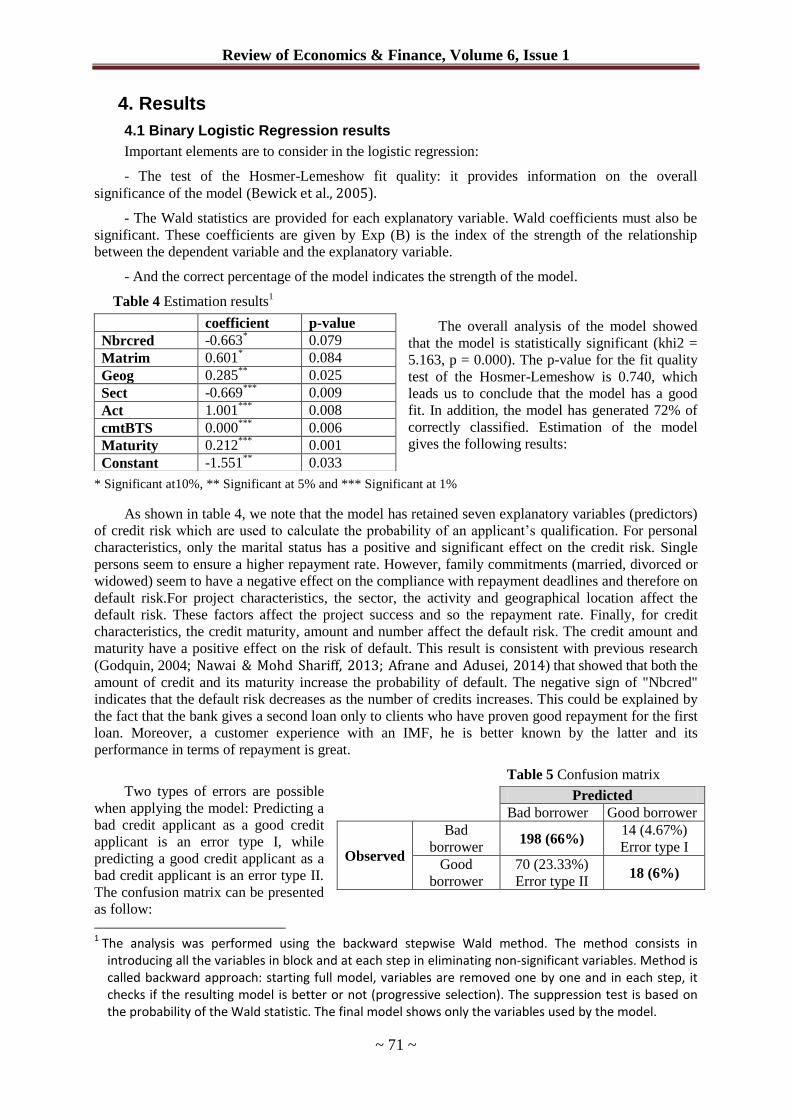
Table 4 Estimation results1

The overall analysis of the model showed

that the model is statistically significant (khi2 =

5.163, p = 0.000). The p-value for the fit quality

test of the Hosmer-Lemeshow is 0.740, which

leads us to conclude that the model has a good

fit. In addition, the model has generated 72% of

correctly classified. Estimation of the model

gives the following results:

* Significant at10%, ** Significant at 5% and *** Significant at 1%

As shown in table 4, we note that the model has retained seven explanatory variables (predictors)

of credit risk which are used to calculate the probability of an applicant’s qualification. For personal

characteristics, only the marital status has a positive and significant effect on the credit risk. Single

persons seem to ensure a higher repayment rate. However, family commitments (married, divorced or

widowed) seem to have a negative effect on the compliance with repayment deadlines and therefore on

default risk.For project characteristics, the sector, the activity and geographical location affect the

default risk. These factors affect the project success and so the repayment rate. Finally, for credit

characteristics, the credit maturity, amount and number affect the default risk. The credit amount and

maturity have a positive effect on the risk of default. This result is consistent with previous research

(Godquin, 2004; Nawai & Mohd Shariff, 2013; Afrane and Adusei, 2014) that showed that both the

amount of credit and its maturity increase the probability of default. The negative sign of "Nbcred"

indicates that the default risk decreases as the number of credits increases. This could be explained by

the fact that the bank gives a second loan only to clients who have proven good repayment for the first

loan. Moreover, a customer experience with an IMF, he is better known by the latter and its

performance in terms of repayment is great.

Table 5 Confusion matrix

Two types of errors are possible

when applying the model: Predicting a

bad credit applicant as a good credit

applicant is an error type I, while

predicting a good credit applicant as a

bad credit applicant is an error type II.

The confusion matrix can be presented

as follow:

1 The analysis was performed using the backward stepwise Wald method. The method consists in

introducing all the variables in block and at each step in eliminating non-significant variables. Method is called backward approach: starting full model, variables are removed one by one and in each step, it checks if the resulting model is better or not (progressive selection). The suppression test is based on the probability of the Wald statistic. The final model shows only the variables used by the model.

coefficient p-value

Nbrcred -0.663* 0.079

Matrim 0.601* 0.084

Geog 0.285**

0.025

Sect -0.669***

0.009

Act 1.001***

0.008

cmtBTS 0.000***

0.006

Maturity 0.212***

0.001

Constant -1.551**

0.033

Predicted

Bad borrower Good borrower

Observed

Bad

borrower 198 (66%)

14 (4.67%)

Error type I

Good

borrower

70 (23.33%)

Error type II 18 (6%)


~ 72 ~

According to Abdou H. et al. (2007), “It is generally believed in a credit scoring application that

the costs associated with both type I and type II errors are significantly different. Generally, the

misclassification cost associated with a type II error is much higher than the misclassification cost

associated with a type I error”. It therefore appears that the logistic regression provides a high type II

error rate (23.33%) compared with Type I error rate (4.67%). A model providing a lower Type II error

rate will be better.

4.2 Artificial Neural Networks results

As a first step and before starting to study, we must prepare the database to make it adequate to

the model. Data pre-processing, called also the scaling of the variables before training, describes any

type of processing performed on raw data to prepare it for another processing procedure. It transforms

the data into a format that will be more easily and effectively processed for the purpose of the user.

Based on normalization as a tool for data pre-processing, it aims to bring back the range of

evolving values taken by variables inside a standardized interval, fixed beforehand. It’s desirable

because it avoids the system to parameterize on a range of specific values, thus ignoring extreme

values. According to Zhang et al. (1999), “data preprocessing is claimed by some authors to be

beneficial for the training of the network”. The main data pre-processing methods used are logarithmic

transformation and normalization. If the series grows exponentially, a logarithmic transformation is

performed. Normalization aims to reduce the range of values taken by the variables within a

standardized range fixed a priori. It is desirable as it avoids the system to set a range of particular

values ignoring outliers. For normalization, we include the two most common methods:

- The first consists to center and reduce the variable. Each observation is transformed as follows:

XX '

X represents the origin observation, the average of the observed variable and its standard

deviation.

- The second used pre-processing consists in a rescaling of variable as follows:

minmax

min'

XX

where, min and max represent respectively, the minimum and the maximum of the variable.

For this study, we apply the second pre-processing since it’s more appropriate in our case. In fact,

our studied variables are with different ranges, rescaling permits to transform the original variable to a

continuous one with the min value 0 and max value 1 (to have variables with the same range).

The determination of the appropriate architecture is essentially dependent of studied problem, the

ANNs conception depends on different parameters, which are determined through experiments, and

namely the number of hidden layers, the number of hidden nodes, the transfer/activation functions and

the learning algorithms. The choice of these parameters plays an important role in model

constructions. Indeed, we have filled a matrix considered as input value with 12 variables in row, and

individual borrowers, providing the learning basis, in column. Also, we built a vector of desired values

(Target) with binary values 0 and 1 which correspond respectively to good and bad applicants.

The data division into training, testing and validation sets is an important step in building ANNs.

An inadequate division of the working sample could affect classification, but there is no general

solution to this issue. For this reason, the experiments were performed using different divisions of the

available data into training, testing, and validation sets, as follows:

- Training set = 90%, testing set = validation set = 5%,




~ 73 ~

The choice of the optimal architecture is based on error performance for different combinations

of parameters indicated above. There are several parameters that can affect the network performance,

like Mean Square Error (MSE), data size, input normalization, data division, momentum, learning rate

and interconnection between neurons. Our first question concerns the effect of data division, hidden

layer number and hidden nodes number on the network performance. We varied the number of hidden

layers between 1 and 2, with the number of hidden units per each hidden layer ranging from 1 to20.

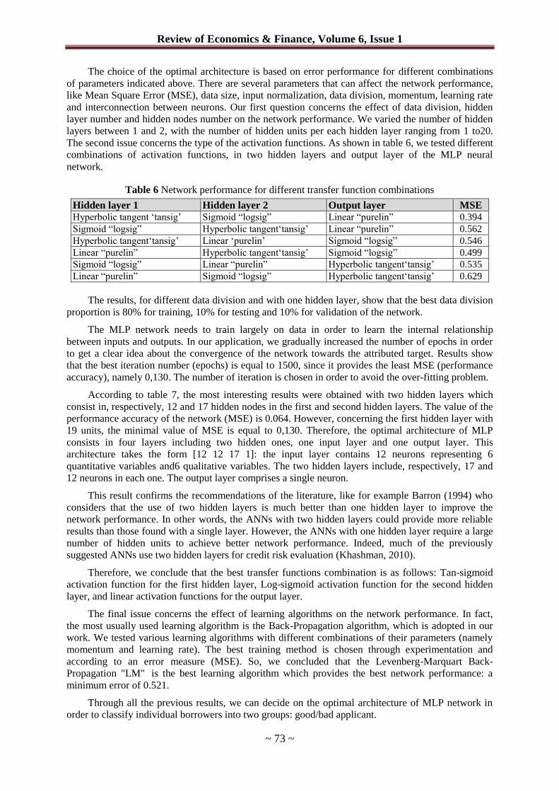
The second issue concerns the type of the activation functions. As shown in table 6, we tested different

combinations of activation functions, in two hidden layers and output layer of the MLP neural

network.

Table 6 Network performance for different transfer function combinations

Hidden layer 1 Hidden layer 2 Output layer MSE

Hyperbolic tangent ‘tansig’ Sigmoid “logsig” Linear “purelin” 0.394

Sigmoid “logsig” Hyperbolic tangent‘tansig’ Linear “purelin” 0.562

Hyperbolic tangent‘tansig’ Linear ‘purelin’ Sigmoid “logsig” 0.546

Linear “purelin” Hyperbolic tangent‘tansig’ Sigmoid “logsig” 0.499

Sigmoid “logsig” Linear “purelin” Hyperbolic tangent‘tansig’ 0.535

Linear “purelin” Sigmoid “logsig” Hyperbolic tangent‘tansig’ 0.629

The results, for different data division and with one hidden layer, show that the best data division

proportion is 80% for training, 10% for testing and 10% for validation of the network.

The MLP network needs to train largely on data in order to learn the internal relationship

between inputs and outputs. In our application, we gradually increased the number of epochs in order

to get a clear idea about the convergence of the network towards the attributed target. Results show

that the best iteration number (epochs) is equal to 1500, since it provides the least MSE (performance

accuracy), namely 0,130. The number of iteration is chosen in order to avoid the over-fitting problem.

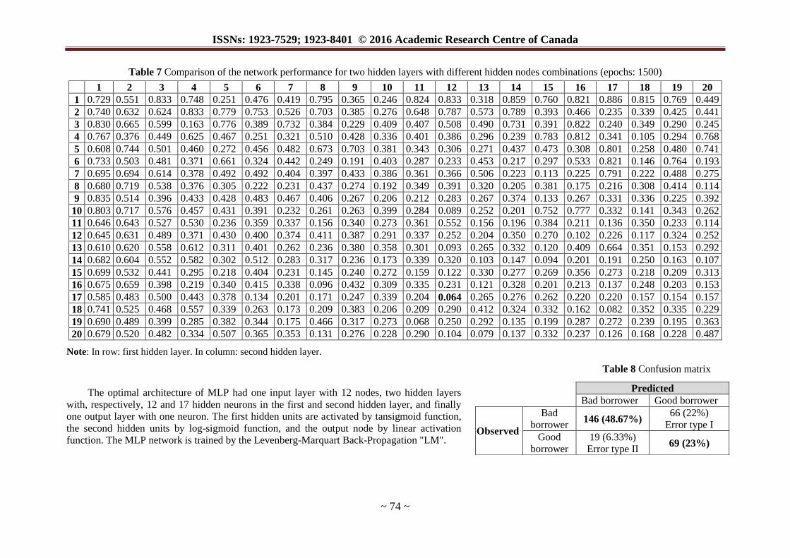
According to table 7, the most interesting results were obtained with two hidden layers which

consist in, respectively, 12 and 17 hidden nodes in the first and second hidden layers. The value of the

performance accuracy of the network (MSE) is 0.064. However, concerning the first hidden layer with

19 units, the minimal value of MSE is equal to 0,130. Therefore, the optimal architecture of MLP

consists in four layers including two hidden ones, one input layer and one output layer. This

architecture takes the form [12 12 17 1]: the input layer contains 12 neurons representing 6

quantitative variables and6 qualitative variables. The two hidden layers include, respectively, 17 and

12 neurons in each one. The output layer comprises a single neuron.

This result confirms the recommendations of the literature, like for example Barron (1994) who

considers that the use of two hidden layers is much better than one hidden layer to improve the

network performance. In other words, the ANNs with two hidden layers could provide more reliable

results than those found with a single layer. However, the ANNs with one hidden layer require a large

number of hidden units to achieve better network performance. Indeed, much of the previously

suggested ANNs use two hidden layers for credit risk evaluation (Khashman, 2010).

Therefore, we conclude that the best transfer functions combination is as follows: Tan-sigmoid

activation function for the first hidden layer, Log-sigmoid activation function for the second hidden

layer, and linear activation functions for the output layer.

The final issue concerns the effect of learning algorithms on the network performance. In fact,

the most usually used learning algorithm is the Back-Propagation algorithm, which is adopted in our

work. We tested various learning algorithms with different combinations of their parameters (namely

momentum and learning rate). The best training method is chosen through experimentation and

according to an error measure (MSE). So, we concluded that the Levenberg-Marquart Back-

Propagation "LM" is the best learning algorithm which provides the best network performance: a

minimum error of 0.521.

Through all the previous results, we can decide on the optimal architecture of MLP network in

order to classify individual borrowers into two groups: good/bad applicant.


~ 74 ~

Table 7 Comparison of the network performance for two hidden layers with different hidden nodes combinations (epochs: 1500)

1 2 3 4 5 6 7 8 9 10 11 12 13 14 15 16 17 18 19 20

1 0.729 0.551 0.833 0.748 0.251 0.476 0.419 0.795 0.365 0.246 0.824 0.833 0.318 0.859 0.760 0.821 0.886 0.815 0.769 0.449

2 0.740 0.632 0.624 0.833 0.779 0.753 0.526 0.703 0.385 0.276 0.648 0.787 0.573 0.789 0.393 0.466 0.235 0.339 0.425 0.441

3 0.830 0.665 0.599 0.163 0.776 0.389 0.732 0.384 0.229 0.409 0.407 0.508 0.490 0.731 0.391 0.822 0.240 0.349 0.290 0.245

4 0.767 0.376 0.449 0.625 0.467 0.251 0.321 0.510 0.428 0.336 0.401 0.386 0.296 0.239 0.783 0.812 0.341 0.105 0.294 0.768

5 0.608 0.744 0.501 0.460 0.272 0.456 0.482 0.673 0.703 0.381 0.343 0.306 0.271 0.437 0.473 0.308 0.801 0.258 0.480 0.741

6 0.733 0.503 0.481 0.371 0.661 0.324 0.442 0.249 0.191 0.403 0.287 0.233 0.453 0.217 0.297 0.533 0.821 0.146 0.764 0.193

7 0.695 0.694 0.614 0.378 0.492 0.492 0.404 0.397 0.433 0.386 0.361 0.366 0.506 0.223 0.113 0.225 0.791 0.222 0.488 0.275

8 0.680 0.719 0.538 0.376 0.305 0.222 0.231 0.437 0.274 0.192 0.349 0.391 0.320 0.205 0.381 0.175 0.216 0.308 0.414 0.114

9 0.835 0.514 0.396 0.433 0.428 0.483 0.467 0.406 0.267 0.206 0.212 0.283 0.267 0.374 0.133 0.267 0.331 0.336 0.225 0.392

10 0.803 0.717 0.576 0.457 0.431 0.391 0.232 0.261 0.263 0.399 0.284 0.089 0.252 0.201 0.752 0.777 0.332 0.141 0.343 0.262

11 0.646 0.643 0.527 0.530 0.236 0.359 0.337 0.156 0.340 0.273 0.361 0.552 0.156 0.196 0.384 0.211 0.136 0.350 0.233 0.114

12 0.645 0.631 0.489 0.371 0.430 0.400 0.374 0.411 0.387 0.291 0.337 0.252 0.204 0.350 0.270 0.102 0.226 0.117 0.324 0.252

13 0.610 0.620 0.558 0.612 0.311 0.401 0.262 0.236 0.380 0.358 0.301 0.093 0.265 0.332 0.120 0.409 0.664 0.351 0.153 0.292

14 0.682 0.604 0.552 0.582 0.302 0.512 0.283 0.317 0.236 0.173 0.339 0.320 0.103 0.147 0.094 0.201 0.191 0.250 0.163 0.107

15 0.699 0.532 0.441 0.295 0.218 0.404 0.231 0.145 0.240 0.272 0.159 0.122 0.330 0.277 0.269 0.356 0.273 0.218 0.209 0.313

16 0.675 0.659 0.398 0.219 0.340 0.415 0.338 0.096 0.432 0.309 0.335 0.231 0.121 0.328 0.201 0.213 0.137 0.248 0.203 0.153

17 0.585 0.483 0.500 0.443 0.378 0.134 0.201 0.171 0.247 0.339 0.204 0.064 0.265 0.276 0.262 0.220 0.220 0.157 0.154 0.157

18 0.741 0.525 0.468 0.557 0.339 0.263 0.173 0.209 0.383 0.206 0.209 0.290 0.412 0.324 0.332 0.162 0.082 0.352 0.335 0.229

19 0.690 0.489 0.399 0.285 0.382 0.344 0.175 0.466 0.317 0.273 0.068 0.250 0.292 0.135 0.199 0.287 0.272 0.239 0.195 0.363

20 0.679 0.520 0.482 0.334 0.507 0.365 0.353 0.131 0.276 0.228 0.290 0.104 0.079 0.137 0.332 0.237 0.126 0.168 0.228 0.487

Note: In row: first hidden layer. In column: second hidden layer.

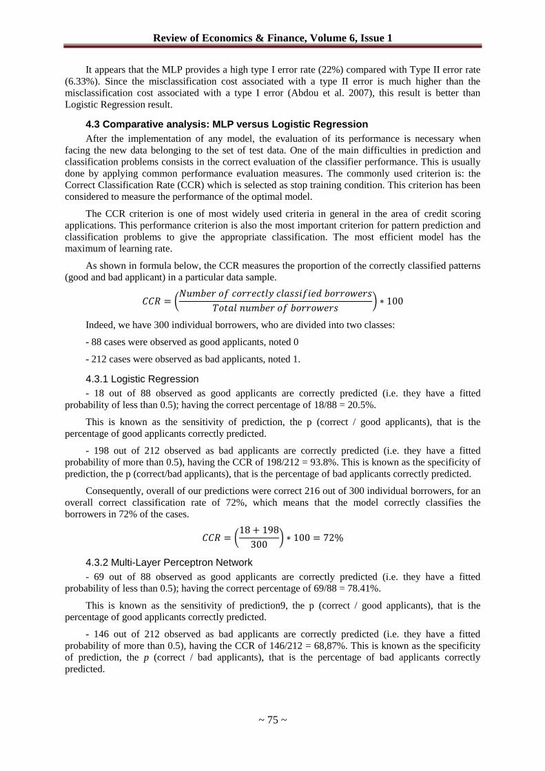
Table 8 Confusion matrix

The optimal architecture of MLP had one input layer with 12 nodes, two hidden layers

with, respectively, 12 and 17 hidden neurons in the first and second hidden layer, and finally

one output layer with one neuron. The first hidden units are activated by tansigmoid function,

the second hidden units by log-sigmoid function, and the output node by linear activation

function. The MLP network is trained by the Levenberg-Marquart Back-Propagation "LM".

Predicted

Bad borrower Good borrower

Observed

Bad

borrower 146 (48.67%)

66 (22%)

Error type I

Good

borrower

19 (6.33%)

Error type II 69 (23%)


~ 75 ~

It appears that the MLP provides a high type I error rate (22%) compared with Type II error rate

(6.33%). Since the misclassification cost associated with a type II error is much higher than the

misclassification cost associated with a type I error (Abdou et al. 2007), this result is better than

Logistic Regression result.

4.3 Comparative analysis: MLP versus Logistic Regression

After the implementation of any model, the evaluation of its performance is necessary when

facing the new data belonging to the set of test data. One of the main difficulties in prediction and

classification problems consists in the correct evaluation of the classifier performance. This is usually

done by applying common performance evaluation measures. The commonly used criterion is: the

Correct Classification Rate (CCR) which is selected as stop training condition. This criterion has been

considered to measure the performance of the optimal model.

The CCR criterion is one of most widely used criteria in general in the area of credit scoring

applications. This performance criterion is also the most important criterion for pattern prediction and

classification problems to give the appropriate classification. The most efficient model has the

maximum of learning rate.

As shown in formula below, the CCR measures the proportion of the correctly classified patterns

(good and bad applicant) in a particular data sample.

Indeed, we have 300 individual borrowers, who are divided into two classes:

- 88 cases were observed as good applicants, noted 0

- 212 cases were observed as bad applicants, noted 1.

4.3.1 Logistic Regression

- 18 out of 88 observed as good applicants are correctly predicted (i.e. they have a fitted

probability of less than 0.5); having the correct percentage of 18/88 = 20.5%.

This is known as the sensitivity of prediction, the p (correct / good applicants), that is the

percentage of good applicants correctly predicted.

- 198 out of 212 observed as bad applicants are correctly predicted (i.e. they have a fitted

probability of more than 0.5), having the CCR of 198/212 = 93.8%. This is known as the specificity of

prediction, the p (correct/bad applicants), that is the percentage of bad applicants correctly predicted.

Consequently, overall of our predictions were correct 216 out of 300 individual borrowers, for an

overall correct classification rate of 72%, which means that the model correctly classifies the

borrowers in 72% of the cases.

4.3.2 Multi-Layer Perceptron Network

- 69 out of 88 observed as good applicants are correctly predicted (i.e. they have a fitted

probability of less than 0.5); having the correct percentage of 69/88 = 78.41%.

This is known as the sensitivity of prediction9, the p (correct / good applicants), that is the

percentage of good applicants correctly predicted.

- 146 out of 212 observed as bad applicants are correctly predicted (i.e. they have a fitted

probability of more than 0.5), having the CCR of 146/212 = 68,87%. This is known as the specificity

of prediction, the p (correct / bad applicants), that is the percentage of bad applicants correctly

predicted.


~ 76 ~

Consequently, most of our predictions were correct 215 out of 300 individual borrowers, for an

overall correct classification rate of 72.2%, which means that the model correctly classifies the

borrowers in 72.2% of the cases.

The efficiency of the constructed models was evaluated by comparing the sensitivity, specificity

and overall correct predictions (CCR) (Padmavathi, 2011). The results are summarized in Table 9.

Table 9 Different performance

measures for MLP and LR

As shown in the table 9, we observed that the logistic regression and the Multi-layer perceptron

(MLP) neural networks give very similar results.

The correct classification percentage (CCR) of the LR is little better than that obtained by MLP,

which shows the performance of the parametric approach. This result is consistent with those found by

Komorád (2009), which concluded the primacy of the classical method "LR" compared to ANNs,

particularly MLP. In fact, his “results indicate that the methods used, namely the logistic regression,

Multi-Layer perceptron (MLP) and radial basis function (RBF) neural networks give very similar

results, however, the traditional Logit model seems to outperform the other techniques”. However, the

sensitivity of Neural Network models (MLP) had a much better predictive power compared to Logistic

Regression. Besides, since the misclassification cost associated with a type II error is much higher

than the misclassification cost associated with a type I error (Abdou et al. 2007), it therefore appears

that the MLP provides better results compared to logistic regression.

5. Conclusion

Credit scoring gains new importance, when thinking about the Basel Capital Accord "Basel II"

extended by "Basel III" which focuses on techniques that allow banks and supervisors to properly

evaluate the various risks that banks face. Thus, credit scoring may contribute to the internal

assessment process of an institution, what is desirable (Komorád, 2009). Credit risk remains the main

concern for banks and other financial institutions, which have put much effort into trying to find the

most effective ways to control or mitigate credit risk.

The assessment of credit risk during the decision to grant credit remains the main concern of

microfinance institutions that have set considerable effort by trying to determine the most effective

ways to make it a task easier to manage, requiring a minimum of time. Credit scoring using a non-

parametric statistical technique with the microfinance industry is a relatively recent application.


approach (MLP) and benchmarks its performance against logistic regression (LR) techniques. Based

on a sample of 300 borrowers from a Tunisian microfinance institution, the results show that logistic

regression and Multi-Layer perceptron (MLP) neural networks give very similar results. On the one

hand, the Correct Classification Rate for LR is little better than that obtained from MLP. On the other

hand, multilayer-perceptron credit scoring allows for lower misclassification costs than LR models. In

fact, the MLP provides an error type II with a reduction of 16.66% in comparison with LR models.

That is, the implementation of a neural network approach supposes that the MFI reduces their losses in

monetary terms. This helps MFIs, as was mentioned by Blanco et al. (2013), “to achieve a competitive

advantage over their competitors”.

As an extension of this study, we can replicate it using other classification methods, such as

Genetic Algorithms, the Bayesian Approach and others to improve the prediction. In addition, a

comparative methodology analysis can also be extended by adding more NN models such as

unsupervised classifiers.

Model CCR (%) Sensitivity (%) Specificity (%)

LR 72 20.5 93.8

MLP 71.67 78.41 68.87


~ 77 ~

References

[1] Abdou H., El-Masry A. and John Pointon (2007). “On the applicability of credit scoring models in

Egyptian banks”, Banks and Bank Systems, 2 (1): 4-20.

[2] Abdou H. and Pointon J. (2011). “Credit scoring, statistical techniques and evaluation criteria: a review

of the literature”, Intelligent Systems in Accounting, Finance & Management, 18 (2-3): 59-88.

[3] Afrane Samuel K. and Michael Adusei (2014). “The Female Superiority in Loan Repayment

Hypothesis: Is it Valid in Ghana?” Advances in Management & Applied Economics, 4 (2): 81-90.

[4] Altman, E.I., Marco, G., Varetto, F. (1994). “Corporate distress diagnosis: Comparisons using linear

discriminant analysis and neural networks (The Italian Experience)”, Journal of Banking and Finance,

18 (3): 505-529.

[5] Anderson R. (2007). The Credit Scoring Toolkit: Theory and Practice for Retail Credit Risk Management and Decision Automation, Oxford University Press, UK.

[6] Andrieş, A. M. (2008). “Theories Regarding the Banking Activity”, Alexandru Ioan Cuza University

Annals, Faculty of Economics and Business Administration, 2008 (55): 19-29.

[7] Bachelet R, Verzat C, Hannachi A et Frugier D. (2004). “Mesurer l'esprit d'entreprendre des élèves

ingénieurs”, 3ème

Congrès de l’Académie de l’Entrepreneuria, Ecole de Management de Lyon,

31mars/01avril : 18 pages (In French).

[8] Bensic M., Sarlija N., Zekic-Susac M. (2005). “Modeling Small Business Credit Scoring by Using

Logistic Regression, Neural Networks, and Decision Trees”, International Journal of Intelligent Systems in Accounting and Finance Management, 13(3): 133-150.

[9] Bewick V, Cheek L, Ball J. (2005). “Statistics review 14: logistic regression”, Critical Care, 9(1): 112-

118.

[10] Blanco Antonio, Rafael Pino-mejías, Juan lara, Salvador Rayo (2013). “Credit scoring models for the

microfinance industry using neural networks: evidence from Peru”, Expert Systems with Applications,

40 (1): 356-364.

[11] Boisselier P., Dufour D. (2003). “Scoring et anticipation de défaillance des entreprises : Une approche

par la régression logistique”, Identification et maîtrise des risques : enjeux pour l’audit, la

comptabilité et le contrôle de gestion, Belgique, pp. 1-20. (In French)

[12] Boissin, J-P, Castagnos J-C et Deschamps B. (2003). “L'intention entrepreneuriale des doctorants“,

colloque intent, Grenoble.

[13] Casu B., Girardone C. and Molyneux P. (2006). Introduction to Banking, Financial Times Press.

[14] Crook J.N., Edelman D.B., Thomas L.C. (2007). “Recent developments in consumer credit risk

assessment”, European Journal of Operational Research, 183 (3): 1447-1465.

[15] Desjardins J. (2005). “L’analyse de régression logistique“, Tutorials in Quantitative Methods for

Psychology, 1(1): 35-41. (In French)

[16] Diallo B. (2006). “Un modèle de Crédit Scoring pour une institution de micro-finance africaine: le cas

de Nuesigiso au Mali“, Laboratoire d’Economie d’Orléans (LEO), Université d’Orléans, pp. 1-48.

[17] Duffie Darrell and Kenneth J. Singleton (2003). Credit Risk: pricing, measurement and management,

Princeton University Press, 416 pages.

[18] Elloumi Awatef, Kammoun Aïda (2013). “Les déterminants de la performance de remboursement des

microcrédits en Tunisie”, Annals of Public and Cooperative Economics, 84(3): 1-21. (In French)

[19] Escaño L.M.E., Saiz G.S., Lorente F.J.L., Fernando Á.B., Ugarriza J.M.V.(2006). “Logistic

Regression Versus Neural Networks For Medical Data”, Monografías del Seminario Matemático

García de Galdeano 33 : 245-252.

[20] Finlay S. (2010). “Credit scoring for profitability objectives”, European Journal of Operational Research, 202(2): 528-537.

[21] Godquin M. (2004). “Microfinance repayment performance in Bangladesh: how to improve the

allocation of loans by IMFs”, World Development, 32 (11): 1909-1926.

[22] Hayden Evelyn and Daniel Porath (2006). “Statistical Methods to Develop Rating Models”, In: Bernd

Engelmann, Robert Rauhmeier (Editors), The Basel II Risk Parameters – Estimation, Validation, and Stress Testing, Springer Verlag, Berlin.


~ 78 ~

[23] Jeatrakul P., Wong K.W. (2009). “Comparing the Performance of Different Neural Networks for

Binary Classification Problems”, Eighth International Symposium on Natural Language Processing,

pp. 111-115.

[24] Khashman A. (2010). “Neural networks for credit risk evaluation: Investigation of different neural

models and learning schemes”, Expert Systems with Applications, 37 (9): 6233-6239.

[25] Klein, Robert W. (1992). “Insurance Company Rating Agencies: A Description of Their Methods and

Procedures”, Kansas City: National Association of Insurance Commissioners.

[26] Komorád Karel (2009). On Credit Scoring Estimation, VDM (Verlag Dr Müller) Edition

[27] Lai K.E., Kuo C.J. (2010). “How to Gauge the Credit Risk of Bank Loans: Evidence from Taiwan”,

International Research Journal of Finance and Economics, 39: 7-14.

[28] Lasch F, Drillon D. et Merdji M. (2004). “Itinéraires de jeunes entrepreneurs : regard sur un dispositif

d'initiation et d'accompagnement à la création d'entreprise”, 3ème Congrès de l’Académie de

l’Entrepreneuriat. Ecole de Management de Lyon, March 31/April 01: 21 pages.

[29] Lee, T.S. & Chen I.F. (2005). “A two-stage hybrid credit scoring model using artificial neural

networks and multivariate adaptive regression splines”, Expert Systems with applications, 28(4): 743-

752.

[30] Matoussi H., Abdelmoula A. (2009). “Using a Neural Network-Based Methodology for Credit—Risk

Evaluation of a Tunisian Bank”, Middle Eastern Finance and Economics, Issue 4, pp. 117-140.

[31] Matoussi H., Abdelmoula A. (2010). “Prévention du risque de défaut dans les banques tunisiennes”,

Crises et nouvelles problématiques de la Valeur, Nice, pp.1-30 (In French).

[32] Mays Elizabeth (2001). Handbook of Credit Scoring, The Glenlake Publishing Company, Ltd.

[33] Muller G. H., Steyn-Bruwer B.W., & Hamman W.D. (2009). “Predicting financial distress of

companies listed on the JSE, comparison of techniques”, South African Journal of Business

Management, 40(1): 21-32

[34] Nawai Norhaziah, and Mohd Shariff (2013). “Determinants of repayment performance in micro-

finance programs in Malaysia”, Labuan Bulletin of International Business & Finance, 11: 14-29.

[35] Ohlson James A. (1980). “Financial Ratios and the probabilistic prediction of bankruptcy”, Journal of

Accounting Research, 18 (1): 109-131.

[36] Padmavathi J. (2011). “A Comparative study on Breast Cancer Prediction Using RBF and MLP”.

International Journal of Scientific & Engineering Research, 2(1) : 1-5.

[37] Rougès V., (2003). “Gestion bancaire du risque de non-remboursement des crédits aux entreprises:

Une revue de littérature“, Centre de Recherche Européen en Finance et Gestion, pp. 1-17. (In French)

[38] Schreiner, M. (2004). “Scoring Arrears at a Micro lender in Bolivia”, Journal of Microfinance, 6(2):

65-88.

[39] Steenackers A., Goovaerts M.J. (1989). “A credit scoring model for Personal loans”, Insurance:

Mathematics and Economics, 8(1): 31-34.

[40] Tseng F.M., Hu Y.C. (2010). “Comparing four bankruptcy prediction models Logit, quadratic interval

logit, neural and fuzzy neural networks”, Expert Systems with Applications, 37(3): 1846-1853.

[41] West D. (2000). “Neural Network Credit Scoring Models”, Computers & Operations Research, 27(11-

12): 1131-1152.

[42] Zhang G., Hu M., Patuwo B.E., Indro D. (1999). “Artificial neural networks in bankruptcy prediction:

General framework and cross-validation analysis”, European Journal of Operational Research, 116

(1): 16-32.

credit scoring models for a tunisian microfinance institution ... · review of economics &...

Documents