CPV in 2HDMSatoru Inoue

(UMass Amherst, ACFI) based on SI, Ramsey-Musolf, Zhang, PRD89, 115023 (2014)

ACFI Workshop, May 1, 2015

Outline

•Intro to 2HDM - motivations and problems

•CP violation in 2HDM

•Collider signatures (briefly)

•EDM tests

•Summary

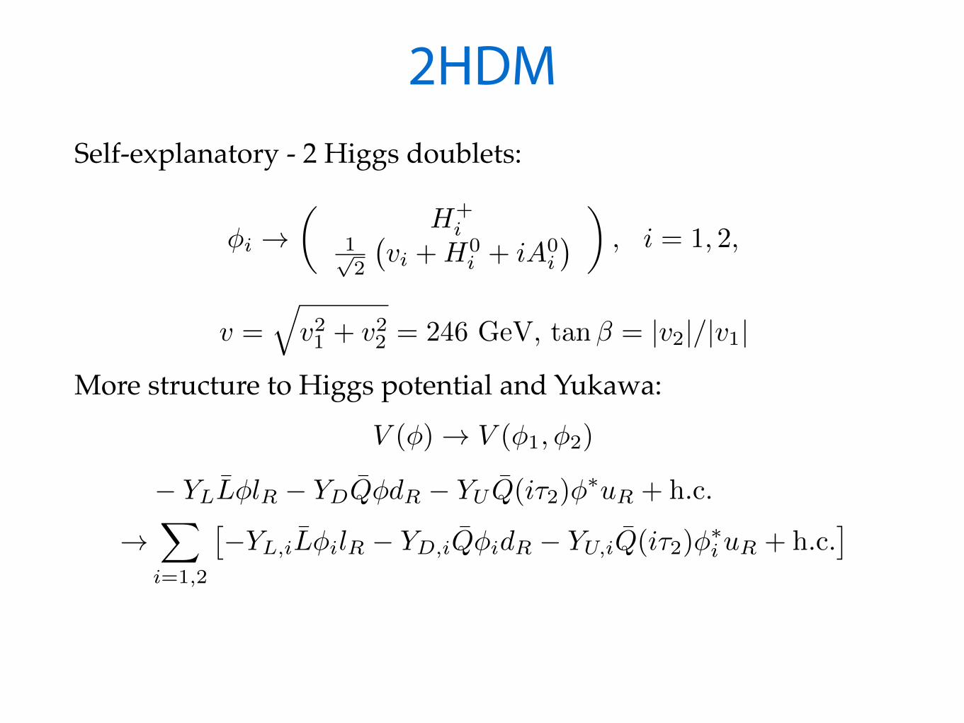
2HDMSelf-explanatory - 2 Higgs doublets:

More structure to Higgs potential and Yukawa:

� YLL̄�lR � YDQ̄�dR � YU Q̄(i⌧2)�⇤uR + h.c.

!X

i=1,2

⇥�YL,iL̄�ilR � YD,iQ̄�idR � YU,iQ̄(i⌧2)�

⇤i uR + h.c.

⇤

v =qv21 + v22 = 246 GeV, tan� = |v2|/|v1|

�i !✓

H+i

1p2

�vi +H0

i + iA0i

�◆, i = 1, 2,

V (�) ! V (�1,�2)

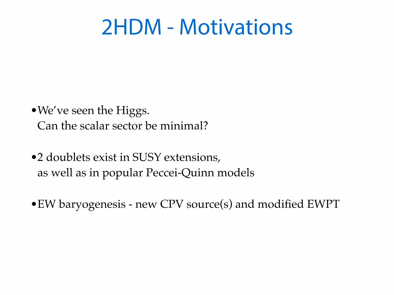
•We’ve seen the Higgs. Can the scalar sector be minimal?

•2 doublets exist in SUSY extensions, as well as in popular Peccei-Quinn models

•EW baryogenesis - new CPV source(s) and modified EWPT

2HDM - Motivations

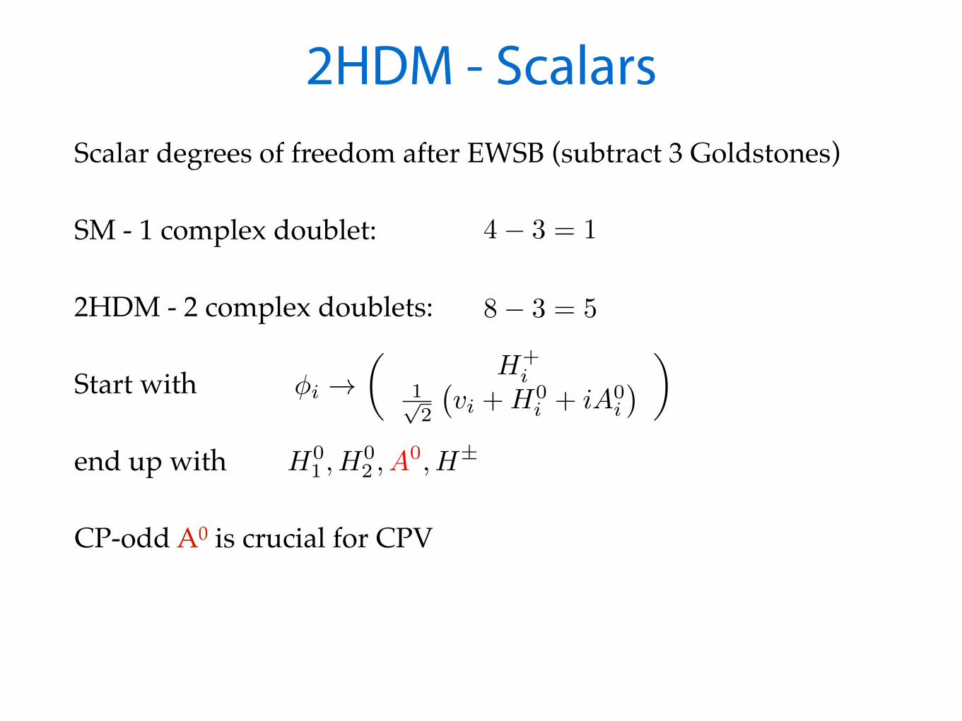
2HDM - ScalarsScalar degrees of freedom after EWSB (subtract 3 Goldstones)

SM - 1 complex doublet:

2HDM - 2 complex doublets:

Start with

end up with

CP-odd A0 is crucial for CPV

4� 3 = 1

8� 3 = 5

�i !✓

H+i

1p2

�vi +H0

i + iA0i

�◆

H01 , H

02 , A

0, H±

Flavor-changing NCSM Yukawa interaction:

Mass matrix ∝ Yukawa:

-> Yukawa is diagonal in mass basis (no tree level FCNC)

General 2HDM:

No simple proportionality:

-> Tree level FCNC (BAD!)

�yij� ̄i j

Mij = vyij/p2

�(y1,ij�1 ̄i j + y2,ij�2 ̄i j)

Mij = (v1y1,ij + v2y2,ij)/p2

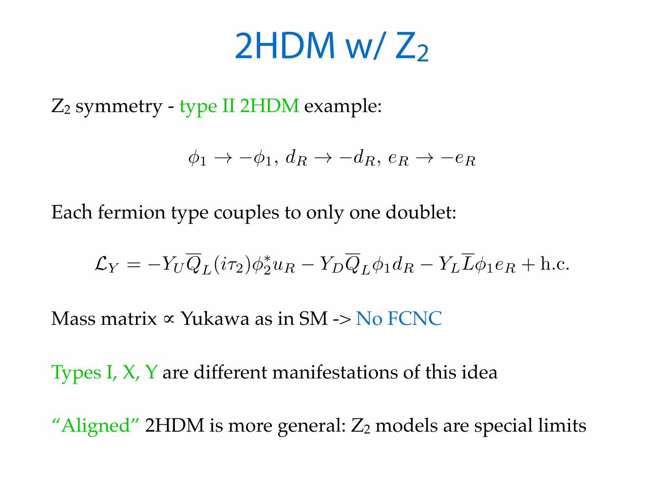
2HDM w/ Z2

Z2 symmetry - type II 2HDM example:

Each fermion type couples to only one doublet:

Mass matrix ∝ Yukawa as in SM -> No FCNC

Types I, X, Y are different manifestations of this idea

“Aligned” 2HDM is more general: Z2 models are special limits

�1 ! ��1, dR ! �dR, eR ! �eR

LY = �YUQL(i⌧2)�⇤2uR � YDQL�1dR � YLL�1eR + h.c.

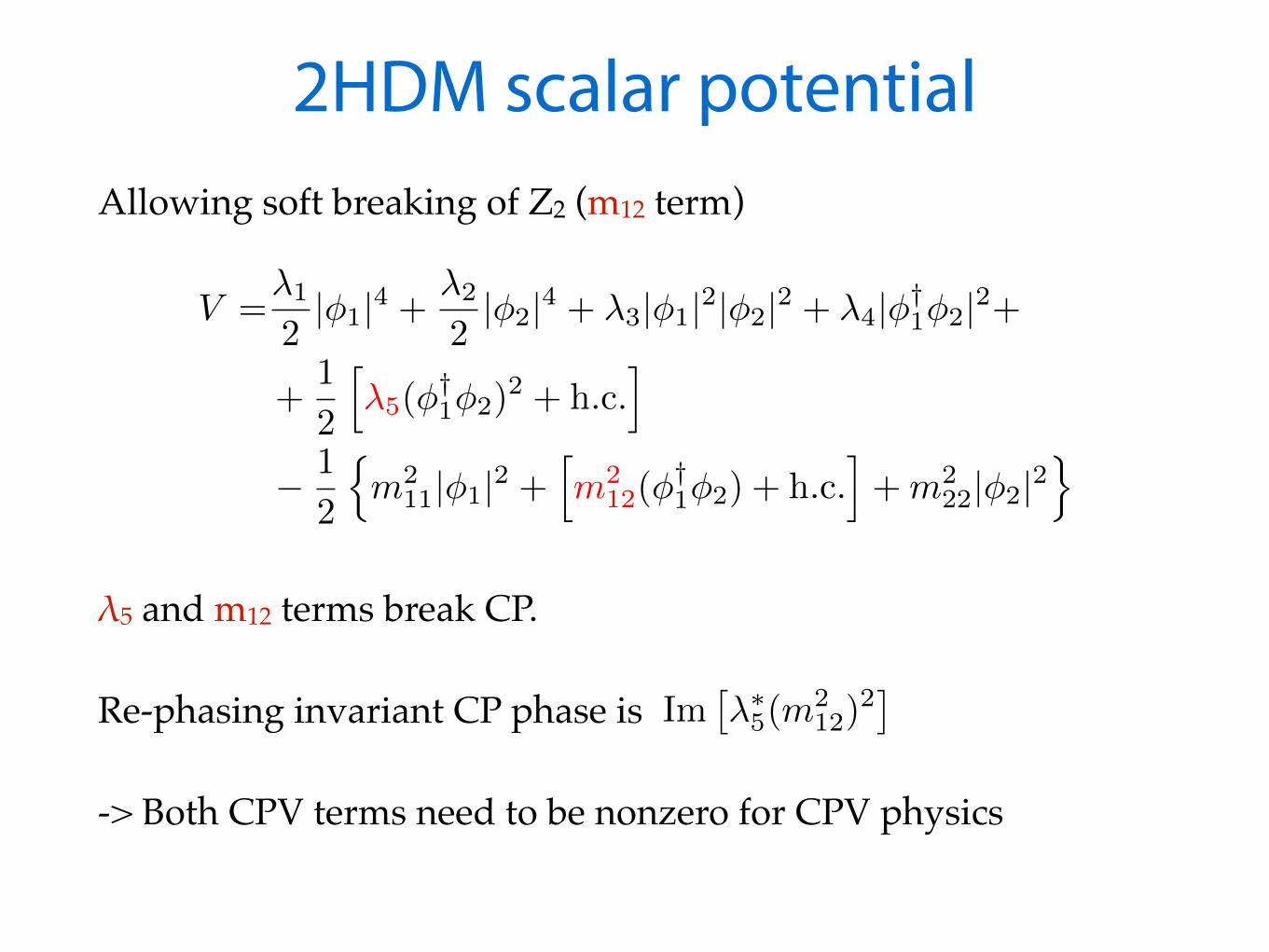
2HDM scalar potentialAllowing soft breaking of Z2 (m12 term)

λ5 and m12 terms break CP.

Re-phasing invariant CP phase is

-> Both CPV terms need to be nonzero for CPV physics

V =�1

2|�1|4 +

�2

2|�2|4 + �3|�1|2|�2|2 + �4|�†

1�2|2+

+1

2

h

�5(�†1�2)

2 + h.c.i

� 1

2

n

m211|�1|2 +

h

m212(�

†1�2) + h.c.

i

+m222|�2|2

o

Im⇥�⇤5(m

212)

2⇤

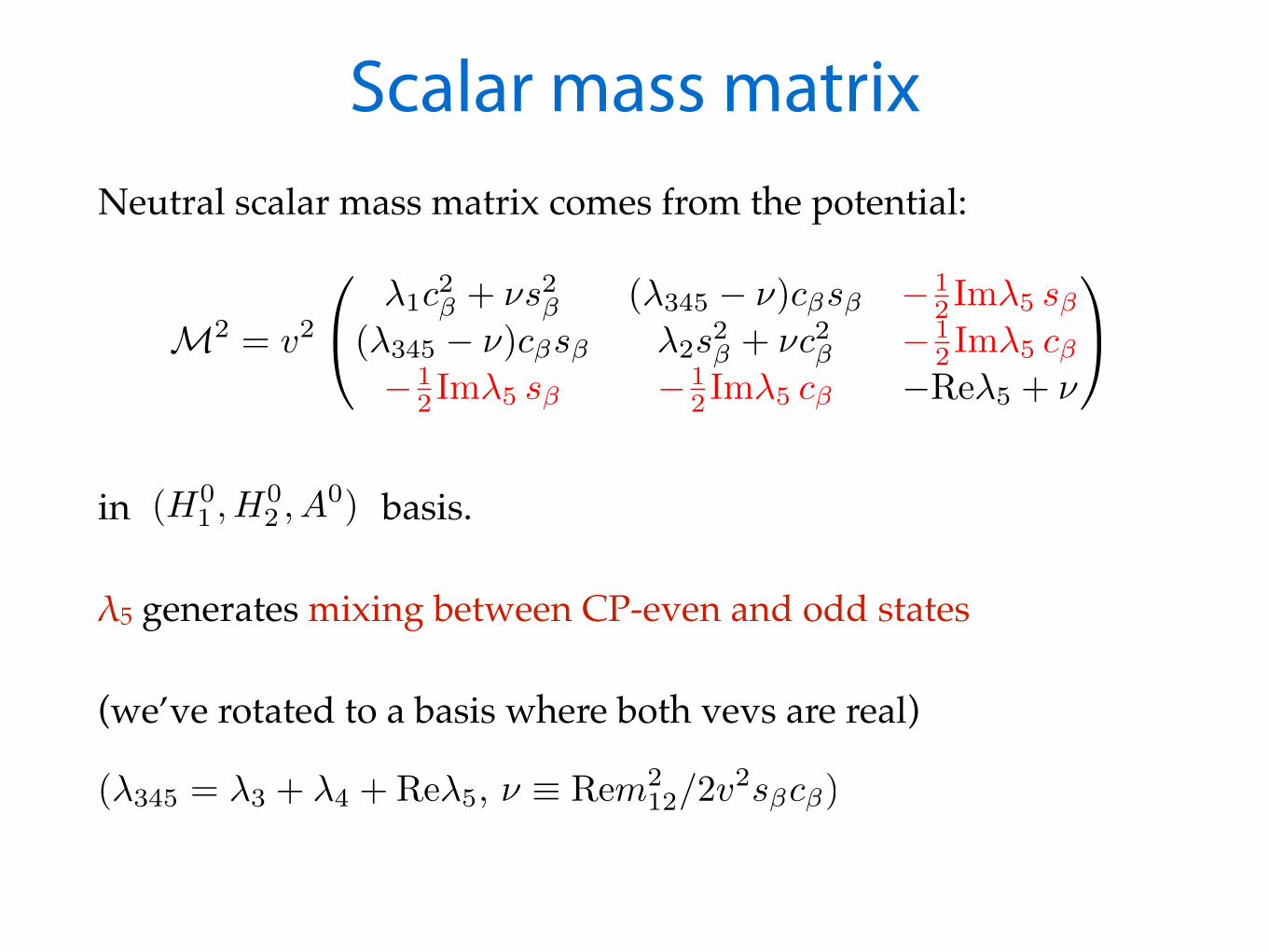
Scalar mass matrixNeutral scalar mass matrix comes from the potential:

in basis.

λ5 generates mixing between CP-even and odd states

(we’ve rotated to a basis where both vevs are real)

M2 = v2

0

@�1c2� + ⌫s2� (�345 � ⌫)c�s� � 1

2 Im�5 s�(�345 � ⌫)c�s� �2s2� + ⌫c2� � 1

2 Im�5 c�� 1

2 Im�5 s� � 12 Im�5 c� �Re�5 + ⌫

1

A

(H01 , H

02 , A

0)

(�345 = �3 + �4 +Re�5, ⌫ ⌘ Rem212/2v

2s�c�)

Higgs mass basis3x3 rotation matrix takes us to mass basis (h1 is 125 GeV Higgs)

Explicitly,

α mixes CP-even states; survives CP-conserving limit

SM-like Yukawas in “aligned” limit (↵ = � � ⇡/2)

0

@h1

h2

h3

1

A = R

0

@H0

1

H02

A0

1

A

R =R23(↵c)R13(↵b)R12(↵+ ⇡/2)

=

0

@�s↵c↵b c↵c↵b s↵b

s↵s↵bs↵c � c↵c↵c �s↵c↵c � c↵s↵bs↵c c↵bs↵c

s↵s↵bc↵c + c↵s↵c s↵s↵c � c↵s↵bc↵c c↵bc↵c

1

A

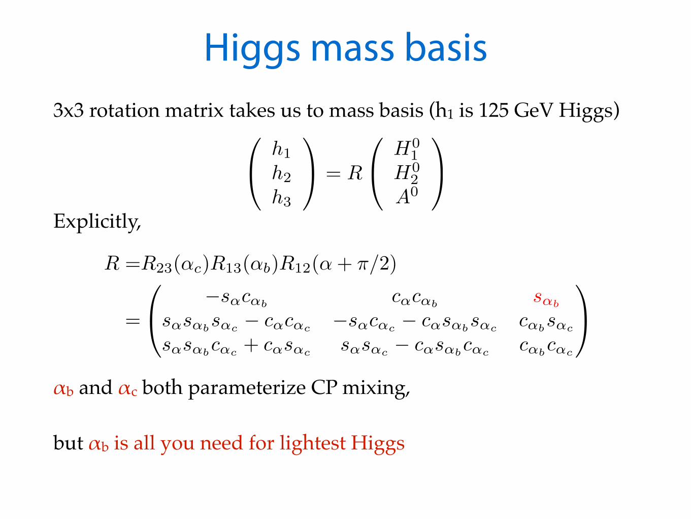
Higgs mass basis3x3 rotation matrix takes us to mass basis (h1 is 125 GeV Higgs)

Explicitly,

αb and αc both parameterize CP mixing,

but αb is all you need for lightest Higgs

R =R23(↵c)R13(↵b)R12(↵+ ⇡/2)

=

0

@�s↵c↵b c↵c↵b s↵b

s↵s↵bs↵c � c↵c↵c �s↵c↵c � c↵s↵bs↵c c↵bs↵c

s↵s↵bc↵c + c↵s↵c s↵s↵c � c↵s↵bc↵c c↵bc↵c

1

A

0

@h1

h2

h3

1

A = R

0

@H0

1

H02

A0

1

A

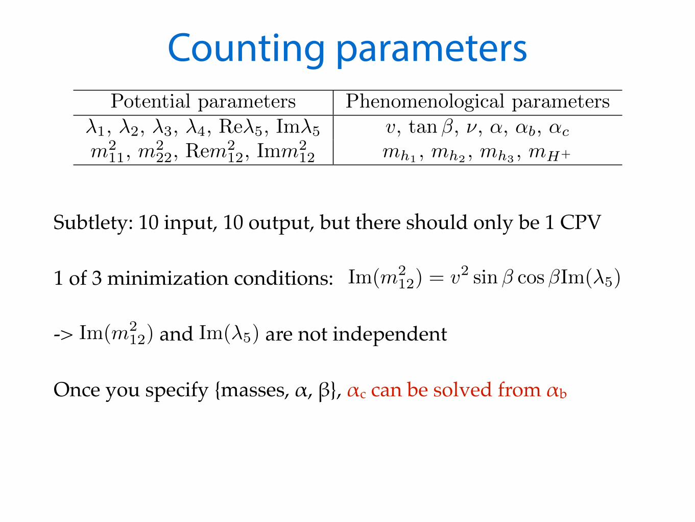
Counting parameters

Subtlety: 10 input, 10 output, but there should only be 1 CPV

1 of 3 minimization conditions:

-> and are not independent

Once you specify {masses, α, β}, αc can be solved from αb

Potential parameters Phenomenological parameters

�1, �2, �3, �4, Re�5, Im�5 v, tan�, ⌫, ↵, ↵b, ↵c

m211, m

222, Rem

212, Imm2

12 mh1 , mh2 , mh3 , mH+

Im(m212) = v2 sin� cos�Im(�5)

Im(m212) Im(�5)

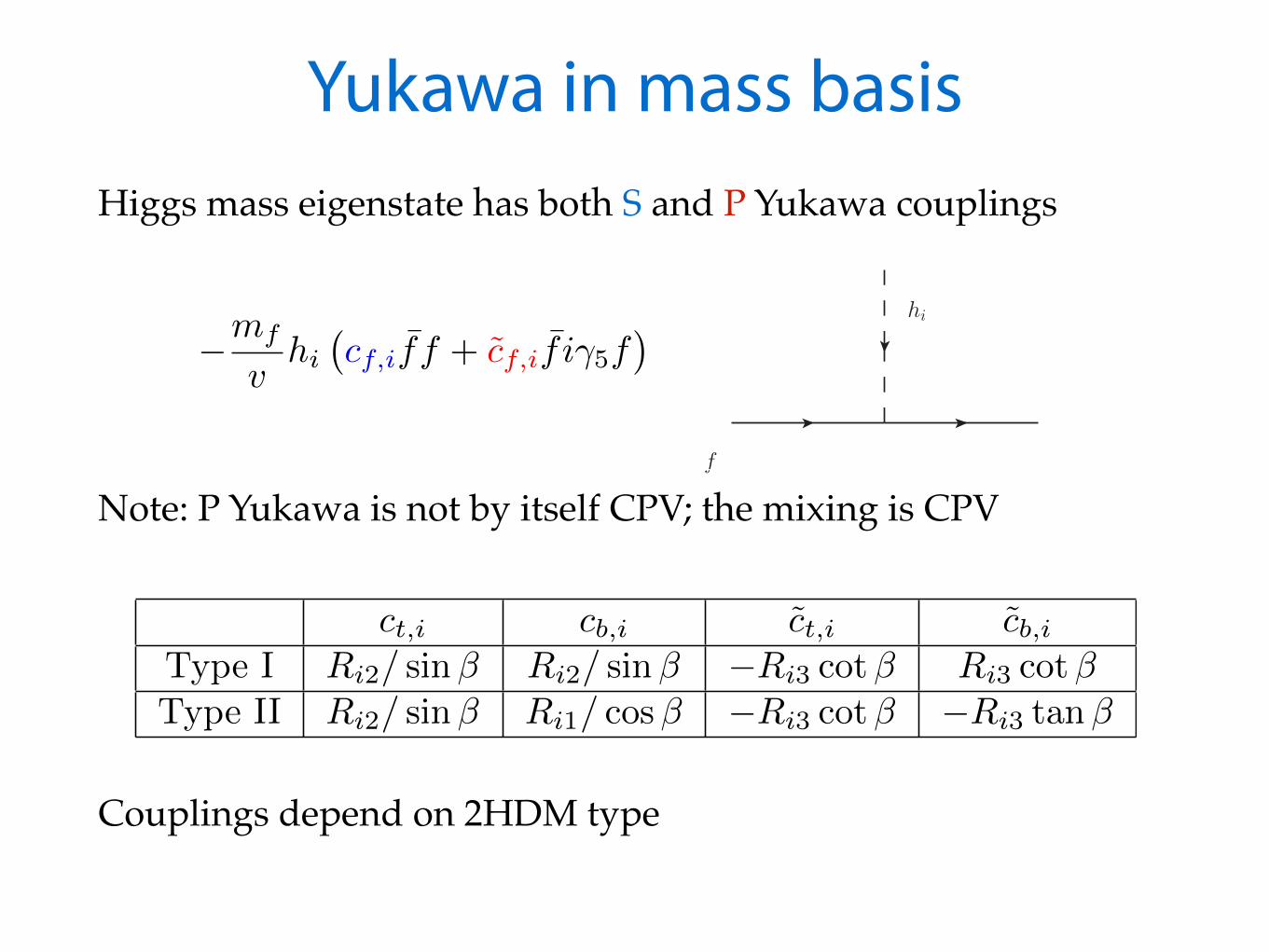
Yukawa in mass basisHiggs mass eigenstate has both S and P Yukawa couplings

Note: P Yukawa is not by itself CPV; the mixing is CPV

Couplings depend on 2HDM type

ct,i cb,i c̃t,i c̃b,iType I Ri2/ sin� Ri2/ sin� �Ri3 cot� Ri3 cot�Type II Ri2/ sin� Ri1/ cos� �Ri3 cot� �Ri3 tan�

f

hi

�mf

vhi

�cf,if̄f + c̃f,if̄ i�5f

�

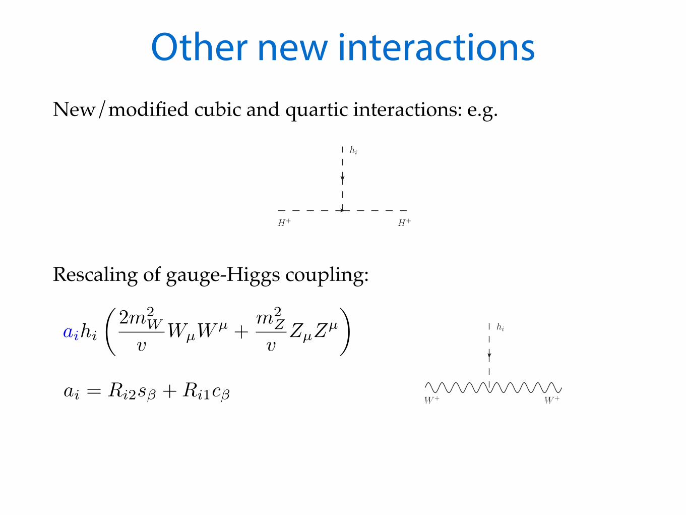
Other new interactionsNew/modified cubic and quartic interactions: e.g.

Rescaling of gauge-Higgs coupling:

H+ H+

hi

aihi

✓2m2

W

vWµW

µ +m2

Z

vZµZ

µ

◆hi

W+ W+ai = Ri2s� +Ri1c�

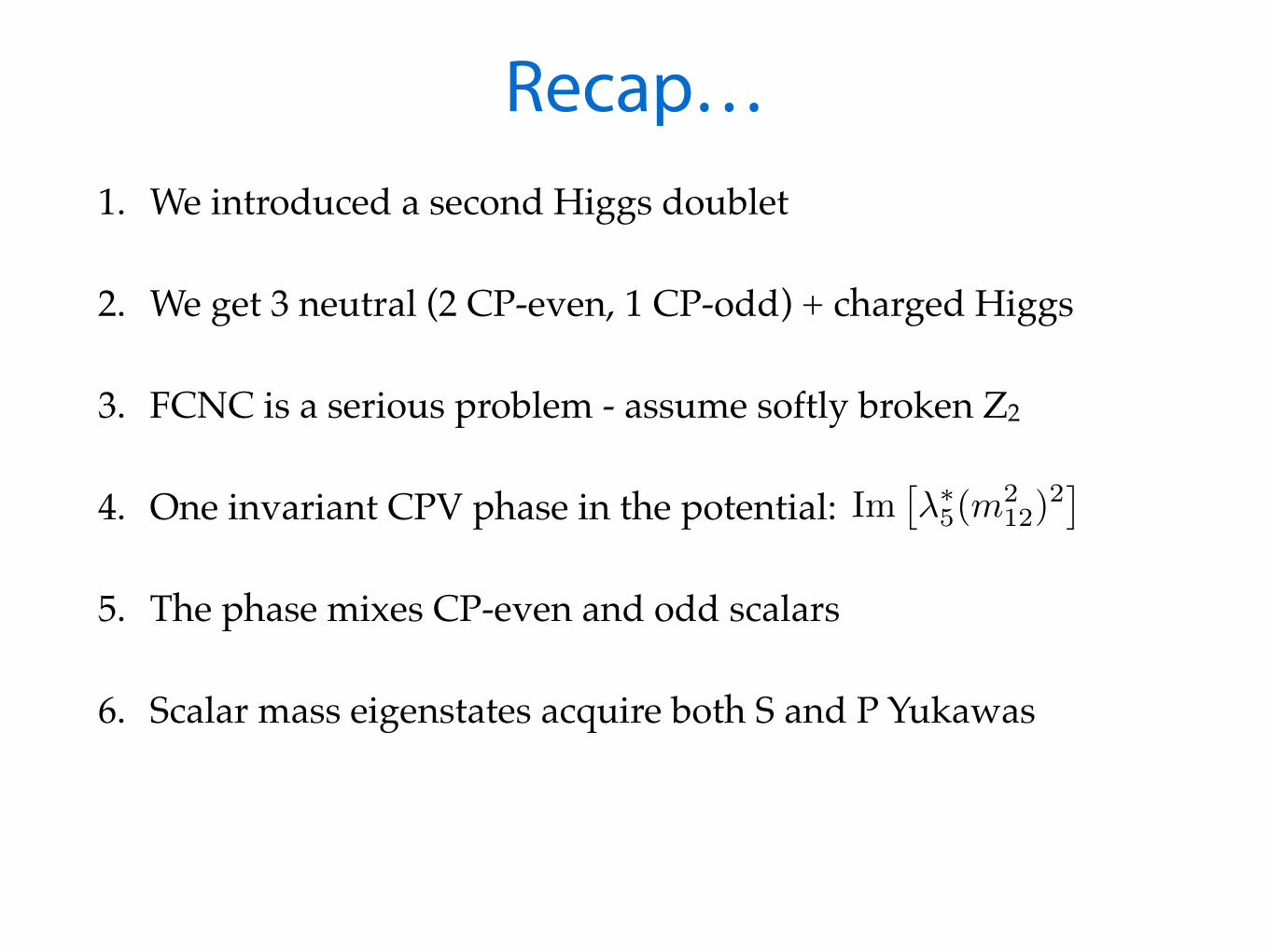
Recap…1. We introduced a second Higgs doublet

2. We get 3 neutral (2 CP-even, 1 CP-odd) + charged Higgs

3. FCNC is a serious problem - assume softly broken Z2

4. One invariant CPV phase in the potential:

5. The phase mixes CP-even and odd scalars

6. Scalar mass eigenstates acquire both S and P Yukawas

Im⇥�⇤5(m

212)

2⇤

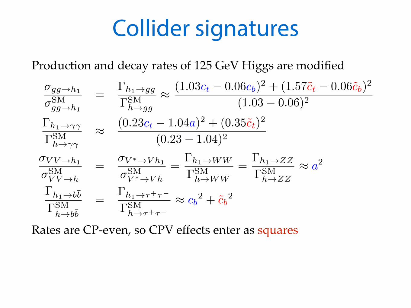
Collider signaturesProduction and decay rates of 125 GeV Higgs are modified

Rates are CP-even, so CPV effects enter as squares

�gg!h1

�SMgg!h1

=�h1!gg

�SMh!gg

⇡ (1.03ct � 0.06cb)2 + (1.57c̃t � 0.06c̃b)2

(1.03� 0.06)2

�h1!��

�SMh!��

⇡ (0.23ct � 1.04a)2 + (0.35c̃t)2

(0.23� 1.04)2

�V V!h1

�SMV V!h

=�V ⇤!V h1

�SMV ⇤!V h

=�h1!WW

�SMh!WW

=�h1!ZZ

�SMh!ZZ

⇡ a2

�h1!bb̄

�SMh!bb̄

=�h1!⌧+⌧�

�SMh!⌧+⌧�

⇡ cb2 + c̃b

2

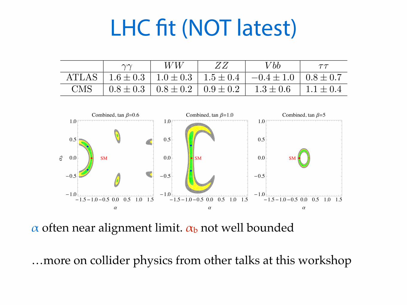
LHC fit (NOT latest)

α often near alignment limit. αb not well bounded

…more on collider physics from other talks at this workshop

SM

-1.5-1.0-0.5 0.0 0.5 1.0 1.5-1.0

-0.5

0.0

0.5

1.0

a

a b

Combined, tan b=0.6

SM

-1.5-1.0-0.5 0.0 0.5 1.0 1.5-1.0

-0.5

0.0

0.5

1.0

a

Combined, tan b=1.0

SM

-1.5-1.0-0.5 0.0 0.5 1.0 1.5-1.0

-0.5

0.0

0.5

1.0

a

Combined, tan b=5

�� WW ZZ V bb ⌧⌧ATLAS 1.6± 0.3 1.0± 0.3 1.5± 0.4 �0.4± 1.0 0.8± 0.7CMS 0.8± 0.3 0.8± 0.2 0.9± 0.2 1.3± 0.6 1.1± 0.4

Current EDM limits (90% CL)electron:

ACME experiment on ThO molecules (2013) - Ongoing

neutron:

(Grenoble 2006) - New experiments in development

mercury:

(Seattle 2009) - New limit soon

radium (this week!): (95% CL)

|dHg| < 2.6⇥ 10�29e cm

|dn| < 2.9⇥ 10�26e cm

|de| < 8.7⇥ 10�28e cm

|dRa| < 5.0⇥ 10�22e cm

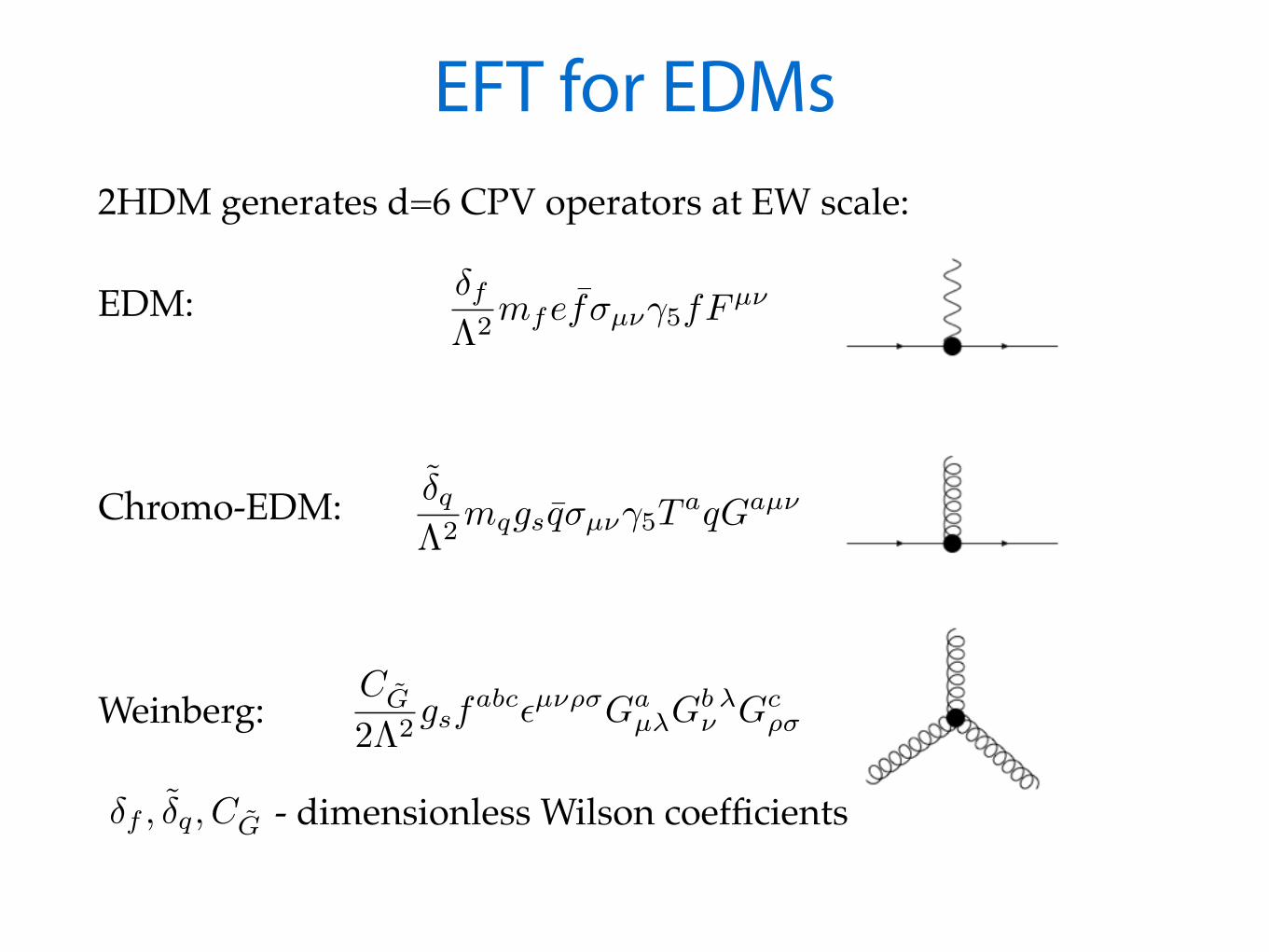
EFT for EDMs2HDM generates d=6 CPV operators at EW scale:

EDM:

Chromo-EDM:

Weinberg:

- dimensionless Wilson coefficients

�f⇤2

mfef̄�µ⌫�5fFµ⌫

�̃q⇤2

mqgsq̄�µ⌫�5TaqGaµ⌫

CG̃

2⇤2gsf

abc✏µ⌫⇢�Gaµ�G

b�⌫ Gc

⇢�

�f , �̃q, CG̃

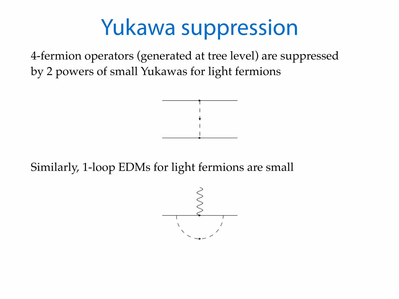
Yukawa suppression4-fermion operators (generated at tree level) are suppressed by 2 powers of small Yukawas for light fermions

Similarly, 1-loop EDMs for light fermions are small

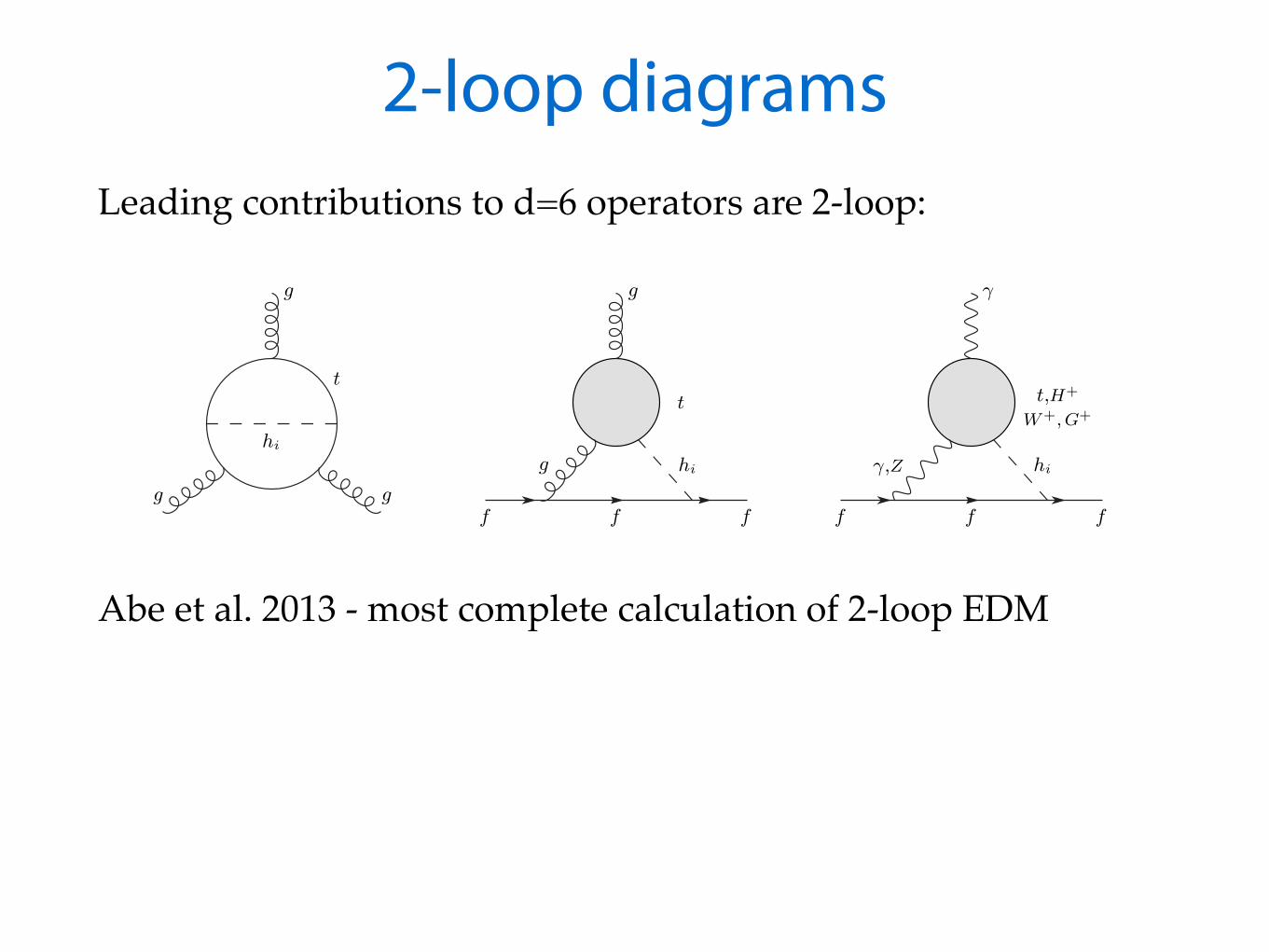
2-loop diagramsLeading contributions to d=6 operators are 2-loop:

Abe et al. 2013 - most complete calculation of 2-loop EDM

hi

g

g g

t

f f f

g

t

g hi

f f f

γ

t,H+

W+, G+

γ,Z hi

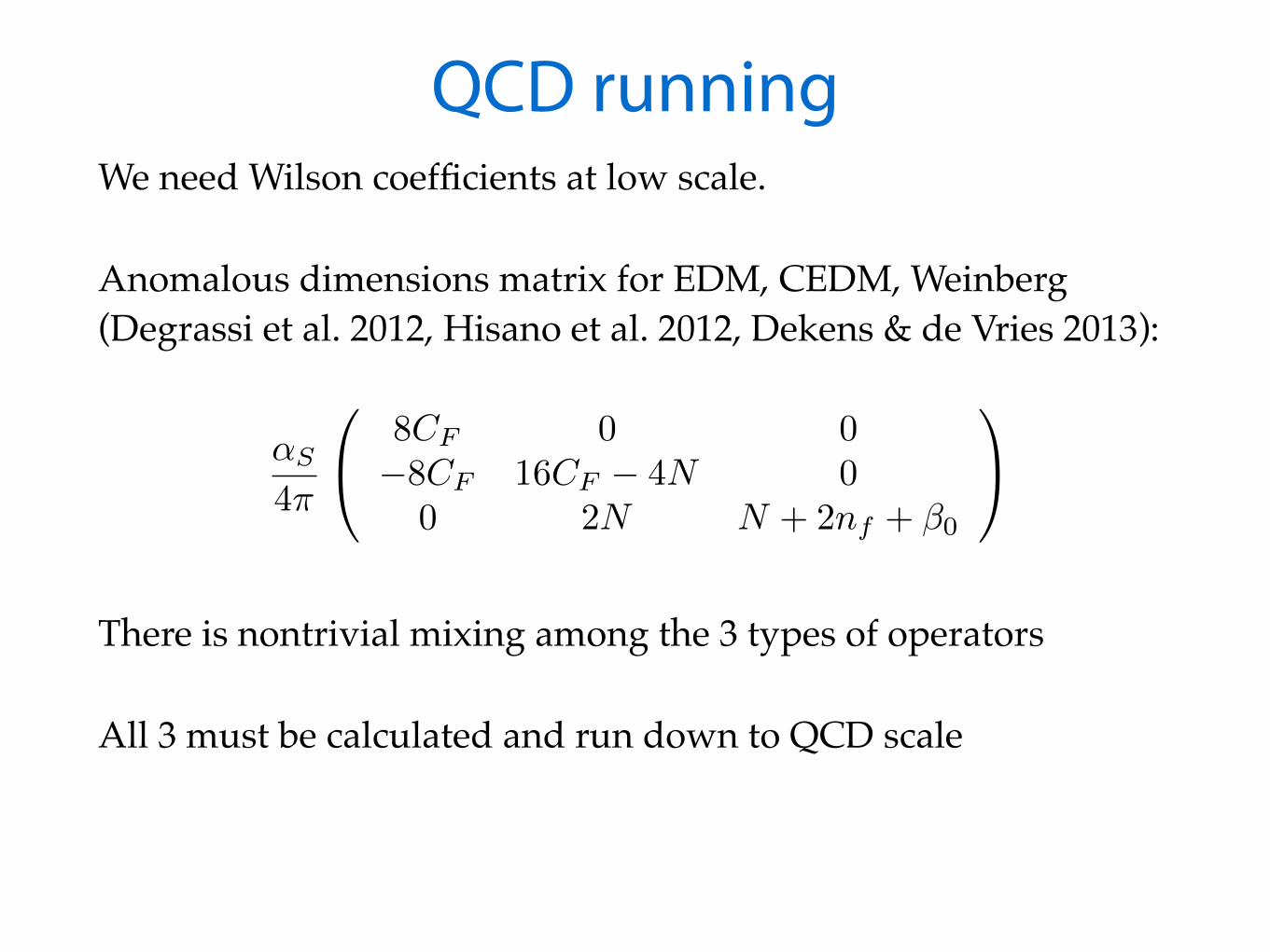
QCD runningWe need Wilson coefficients at low scale.

Anomalous dimensions matrix for EDM, CEDM, Weinberg (Degrassi et al. 2012, Hisano et al. 2012, Dekens & de Vries 2013):

There is nontrivial mixing among the 3 types of operators

All 3 must be calculated and run down to QCD scale

↵S

4⇡

0

@8CF 0 0�8CF 16CF � 4N 0

0 2N N + 2nf + �0

1

A

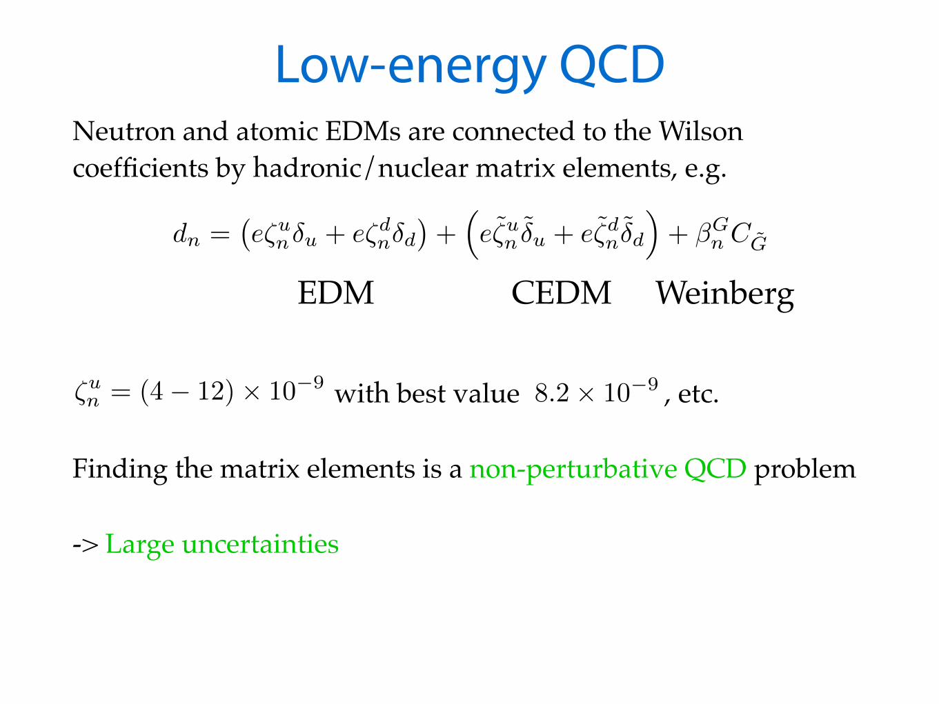
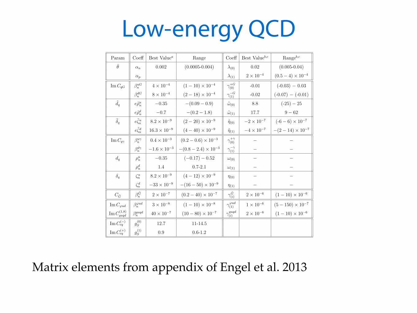
Low-energy QCDNeutron and atomic EDMs are connected to the Wilson coefficients by hadronic/nuclear matrix elements, e.g.

with best value , etc.

Finding the matrix elements is a non-perturbative QCD problem

-> Large uncertainties

dn =�e⇣un�u + e⇣dn�d

�+

⇣e⇣̃un �̃u + e⇣̃dn�̃d

⌘+ �G

n CG̃

EDM CEDM Weinberg

⇣un = (4� 12)⇥ 10�9 8.2⇥ 10�9

Low-energy QCD

Matrix elements from appendix of Engel et al. 2013

Param Coe↵ Best Valuea Range Coe↵ Best Valueb,c Rangeb,c

✓̄ ↵n 0.002 (0.0005-0.004) �(0) 0.02 (0.005-0.04)

↵p �(1) 2⇥ 10�4 (0.5� 4)⇥ 10�4

ImCqG �uGn 4⇥ 10�4 (1� 10)⇥ 10�4 �+G

(0) -0.01 (-0.03) � 0.03

�dGn 8⇥ 10�4 (2� 18)⇥ 10�4 ��G

(1) -0.02 (-0.07) � (-0.01)

d̃q e⇢̃un �0.35 �(0.09� 0.9) !̃(0) 8.8 (-25)� 25

e⇢̃dn �0.7 �(0.2� 1.8) !̃(1) 17.7 9� 62

�̃q e⇣̃un 8.2⇥ 10�9 (2� 20)⇥ 10�9 ⌘̃(0) �2⇥ 10�7 (-6� 6)⇥ 10�7

e⇣̃dn 16.3⇥ 10�9 (4� 40)⇥ 10�9 ⌘̃(1) �4⇥ 10�7 �(2� 14)⇥ 10�7

ImCq� �u�n 0.4⇥ 10�3 (0.2� 0.6)⇥ 10�3 �+�

(0) � ��d�n �1.6⇥ 10�3 �(0.8� 2.4)⇥ 10�3 ���

(1) � �

dq ⇢un �0.35 (�0.17)� 0.52 !(0) � �⇢dn 1.4 0.7-2.1 !(1) � �

�q ⇣un 8.2⇥ 10�9 (4� 12)⇥ 10�9 ⌘(0) � �⇣dn �33⇥ 10�9 �(16� 50)⇥ 10�9 ⌘(1) � �

CG̃ �G̃n 2⇥ 10�7 (0.2� 40)⇥ 10�7 �G̃

(i) 2⇥ 10�6 (1� 10)⇥ 10�6

ImC'ud �'udn 3⇥ 10�8 (1� 10)⇥ 10�8 �'ud

(1) 1⇥ 10�6 (5� 150)⇥ 10�7

ImC(1,8)quqd �quqd

n 40⇥ 10�7 (10� 80)⇥ 10�7 �quqd(i) 2⇥ 10�6 (1� 10)⇥ 10�6

ImC(�)eq g(0)S 12.7 11-14.5

ImC(+)eq g(1)S 0.9 0.6-1.2

Table 6: Best values and reasonable ranges for hadronic matrix elements of CPV operators. Firstcolumn indicates the coe�cient of the operator in the CPV Lagrangian, while second column indicatesthe hadronic matrix element (sensitivity coe�cient) governing its manifestation to the neutron EDM.Third and fourth columns give the best values and reasonable ranges for these hadronic coe�cients.Firth to seventh columns give corresponding result for contributions to TVPV ⇡NN couplings. a Unitsare e fm for all but the ⇢̃qn and ⇢qn.

b We do not list entries for (�±�(i) , !(i), ⌘(i)) as they are suppressed by

↵/⇡ with respect to (�̃±�(i) , !̃(i), ⌘̃(i)) . c The !̃(0,1) are in units of fm�1.

74

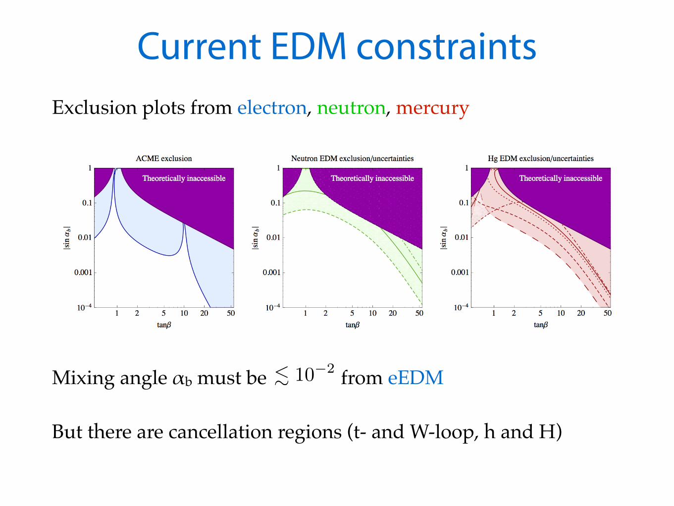
Current EDM constraintsExclusion plots from electron, neutron, mercury

Mixing angle αb must be from eEDM

But there are cancellation regions (t- and W-loop, h and H)

. 10�2

15

FIG. 6: Current constraints from the electron EDM (left), neutron EDM (middle) and 199Hg EDM (right).First row: type-Imodel; Second row: type-II model. In all the plots, we have imposed the condition that ↵ = � � ⇡/2. The other parametersare chosen to be mH+ = 420 GeV, mh2 = 400 GeV, mh3 = 450 GeV and ⌫ = 1.0. Again, ↵c is a dependent parametersolved using Eq. (43). The purple region is theoretically not accessible because Eq. (43) does not have a real solution. Forthe neutron and Mercury EDMs, theoretical uncertainties from hadronic and nuclear matrix elements are reflected by di↵erentcurves. For the neutron EDM, we vary one of the most important hadronic matrix elements: ⇣̃d

n = 1.63 ⇥ 10�8 (solid, centralvalue), 0.4 ⇥ 10�8 (dot-dashed) and 4.0 ⇥ 10�8 (dashed). For the Mercury EDM, we take di↵erent sets of nuclear matrixelement values: a0 = 0.01, a1 = 0.02 (solid, central value). a0 = 0.01, a1 = 0.09 (long-dashed), a0 = 0.01, a1 = �0.03 (dashed),a0 = 0.005, a1 = 0.02 (dotted) and a0 = 0.05, a1 = 0.02 (dot-dashed).

H�� contributions. As we will show below, these cancellation regions can be closed when the neutron and mercuryEDM limits are taken into account. A generic feature is that for growing tan�, the EDM constraints become weakerin the type-I 2HDM, but become stronger in the type-II 2HDM, which can be understood from the tan� dependencesin Eq. (27).

C. Ine↵ectiveness of a Light-Higgs-Only Theory

From the discussion of electron EDM, we have learned that the heavy Higgs contributions via H�� and H±W⌥�diagrams make non-negligible contributions to the total EDM. They can even be dominant at large tan� & 20. Thisexample illustrates the ine↵ectiveness of the “light Higgs e↵ective theory”, often performed as model independentanalyses, which include the CPV e↵ects only from the lightest Higgs (mass 125 GeV). The key point is that a CPviolating Higgs sector usually contains more than one scalar at the electroweak scale, and all of them have CPVinteractions in general. The total contribution therefore includes CPV e↵ects from not only CP even-odd neutralscalar mixings, but also the CPV neutral-charged scalar interactions from the Higgs potential. This is necessarilymodel dependent. In this work, we have included the complete contributions to EDMs in the flavor-conserving (type-Iand type-II) 2HDMs .

Current EDM constraintsExclusion plots from electron, neutron, mercury

Different lines for n & Hg: possible values of matrix elements

~order of magnitude uncertainty in low energy QCD

15

FIG. 6: Current constraints from the electron EDM (left), neutron EDM (middle) and 199Hg EDM (right).First row: type-Imodel; Second row: type-II model. In all the plots, we have imposed the condition that ↵ = � � ⇡/2. The other parametersare chosen to be mH+ = 420 GeV, mh2 = 400 GeV, mh3 = 450 GeV and ⌫ = 1.0. Again, ↵c is a dependent parametersolved using Eq. (43). The purple region is theoretically not accessible because Eq. (43) does not have a real solution. Forthe neutron and Mercury EDMs, theoretical uncertainties from hadronic and nuclear matrix elements are reflected by di↵erentcurves. For the neutron EDM, we vary one of the most important hadronic matrix elements: ⇣̃d

n = 1.63 ⇥ 10�8 (solid, centralvalue), 0.4 ⇥ 10�8 (dot-dashed) and 4.0 ⇥ 10�8 (dashed). For the Mercury EDM, we take di↵erent sets of nuclear matrixelement values: a0 = 0.01, a1 = 0.02 (solid, central value). a0 = 0.01, a1 = 0.09 (long-dashed), a0 = 0.01, a1 = �0.03 (dashed),a0 = 0.005, a1 = 0.02 (dotted) and a0 = 0.05, a1 = 0.02 (dot-dashed).

H�� contributions. As we will show below, these cancellation regions can be closed when the neutron and mercuryEDM limits are taken into account. A generic feature is that for growing tan�, the EDM constraints become weakerin the type-I 2HDM, but become stronger in the type-II 2HDM, which can be understood from the tan� dependencesin Eq. (27).

C. Ine↵ectiveness of a Light-Higgs-Only Theory

From the discussion of electron EDM, we have learned that the heavy Higgs contributions via H�� and H±W⌥�diagrams make non-negligible contributions to the total EDM. They can even be dominant at large tan� & 20. Thisexample illustrates the ine↵ectiveness of the “light Higgs e↵ective theory”, often performed as model independentanalyses, which include the CPV e↵ects only from the lightest Higgs (mass 125 GeV). The key point is that a CPviolating Higgs sector usually contains more than one scalar at the electroweak scale, and all of them have CPVinteractions in general. The total contribution therefore includes CPV e↵ects from not only CP even-odd neutralscalar mixings, but also the CPV neutral-charged scalar interactions from the Higgs potential. This is necessarilymodel dependent. In this work, we have included the complete contributions to EDMs in the flavor-conserving (type-Iand type-II) 2HDMs .

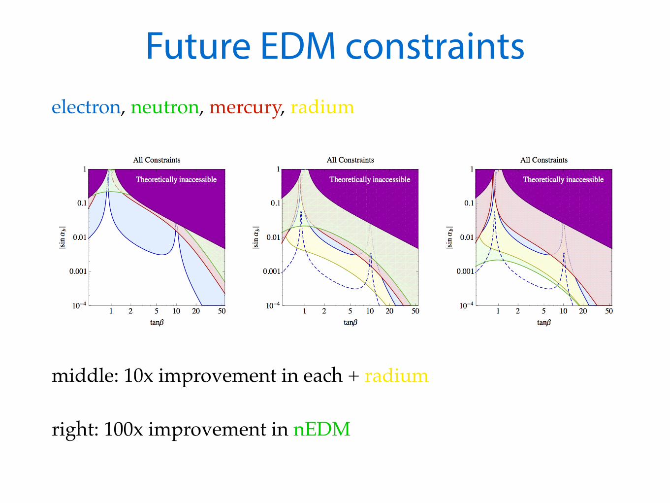
Future EDM constraintselectron, neutron, mercury, radium

middle: 10x improvement in each + radium

right: 100x improvement in nEDM

19

FIG. 10: Current and prospective future constraints from electron EDM (blue), neutron EDM (green), Mercury EDM (red) andRadium (yellow) in flavor conserving 2HDMs. First row: type-I model; Second row: type-II model. The model parametersused are the same as Fig. 6. Central values of the hadronic and nuclear matrix elements are used. Left: Combined currentlimits. Middle: combined future limits if the Mercury and neutron EDMs are both improved by one order of magnitude. Alsoshown are the future constraints if electron EDM is improved by another order of magnitude (in blue dashed curves). Right:combined future limits if the Mercury and neutron EDMs are improved by one and two orders of magnitude, respectively.

V. SUMMARY

The nature of CPV beyond the Standard Model remains a question at the forefront of fundamental physics. Thecosmic matter-antimatter asymmetry strongly implies that such BSM CPV should exist, but the associated mass scaleand dynamics remain unknown. With the observation of the 125 GeV boson at the LHC, it is particularly interestingto ask whether the scalar sector of the larger framework containing the SM admits new sources of CPV and, if so,whether their e↵ects are experimentally accessible. In this study, we have explored this question in the context offlavor conserving 2HDMs, allowing for a new source of CPV in the scalar potential. The present constraints on thistype of CPV are generally weaker than for scenarios where the BSM directly enters the couplings to SM fermions, asthe associated contributions to electric dipole moments generically first appear at two-loop order. In this context, wefind that present EDM limits are complementary to scalar sector constraints from LHC results, as the latter generallyconstrain the CP-conserving sector of the type-I and type-II models, whereas EDMs probe the CPV parameter space.Moreover, despite the additional loop suppression, the present ThO, 199Hg, and neutron EDM search constraints arequite severe, limiting | sin↵b| to ⇠ 0.01 or smaller for most values of tan�.

The next generation of EDM searches could extend the present reach by an order of magnitude or more and couldallow one to distinguish between the type-I and type-II models. In particular, a non-zero neutron or diamagneticatom EDM result would likely point to the type-II model, as even the present ThO limit precludes an observablee↵ect in the type-I scenario given the planned sensitivity of the neutron and diamagnetic atom searches. Furthermore,

Summary

• 2HDM is a well-motivated framework to explore CPV Higgs

• New CPV source results in CP mixing of scalars

• LHC results mainly constrain CP-conserving angle α

• EDMs constrain CP mixing angle αb to ~10-2

• Electron EDMs currently put tightest bounds, but others can become competitive in the foreseeable future

• …but hadronic uncertainties are troublesome

Backup

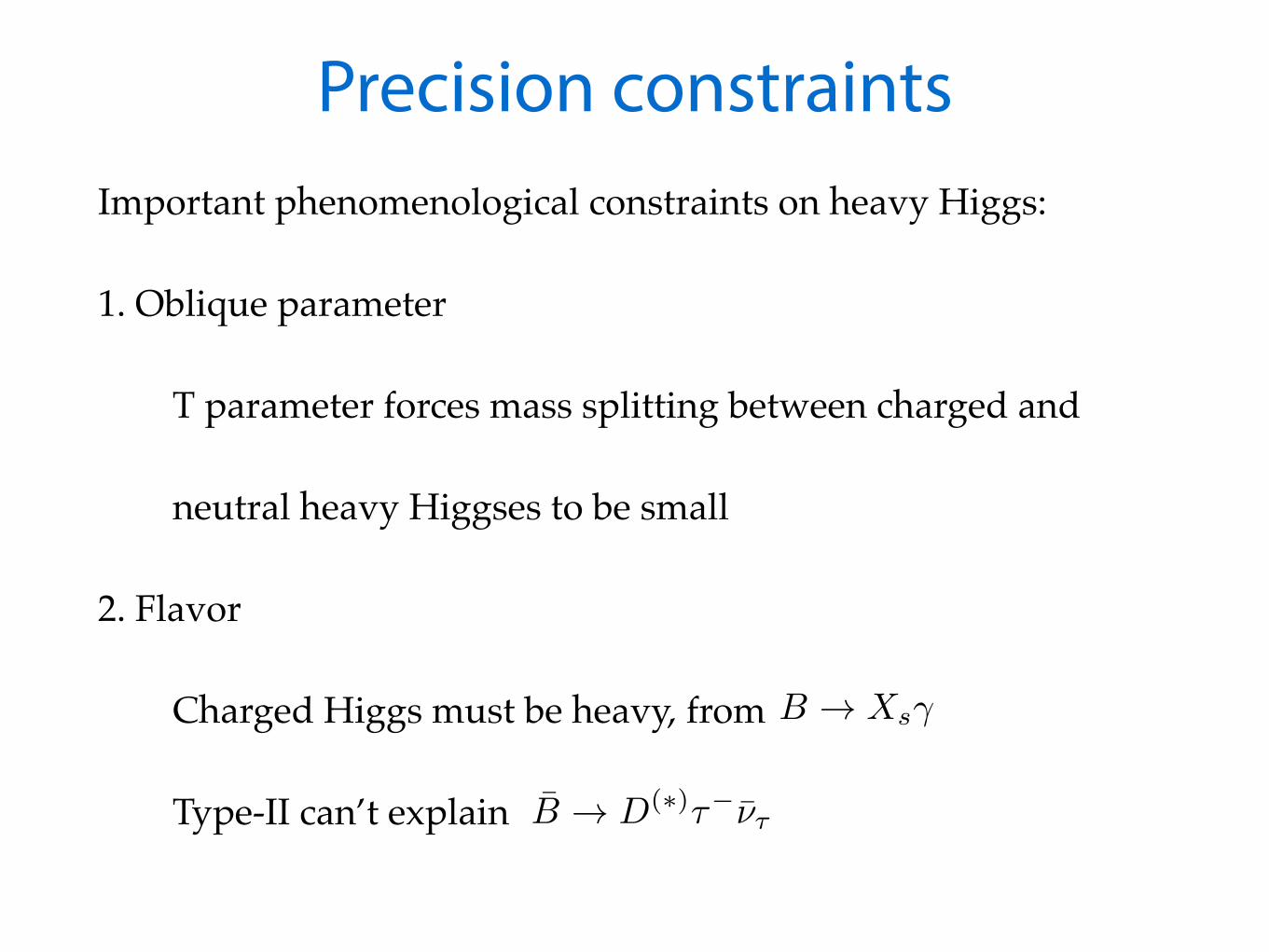
Precision constraintsImportant phenomenological constraints on heavy Higgs:

1. Oblique parameter

T parameter forces mass splitting between charged and

neutral heavy Higgses to be small

2. Flavor

Charged Higgs must be heavy, from

Type-II can’t explain

B ! Xs�

B̄ ! D(⇤)⌧�⌫̄⌧

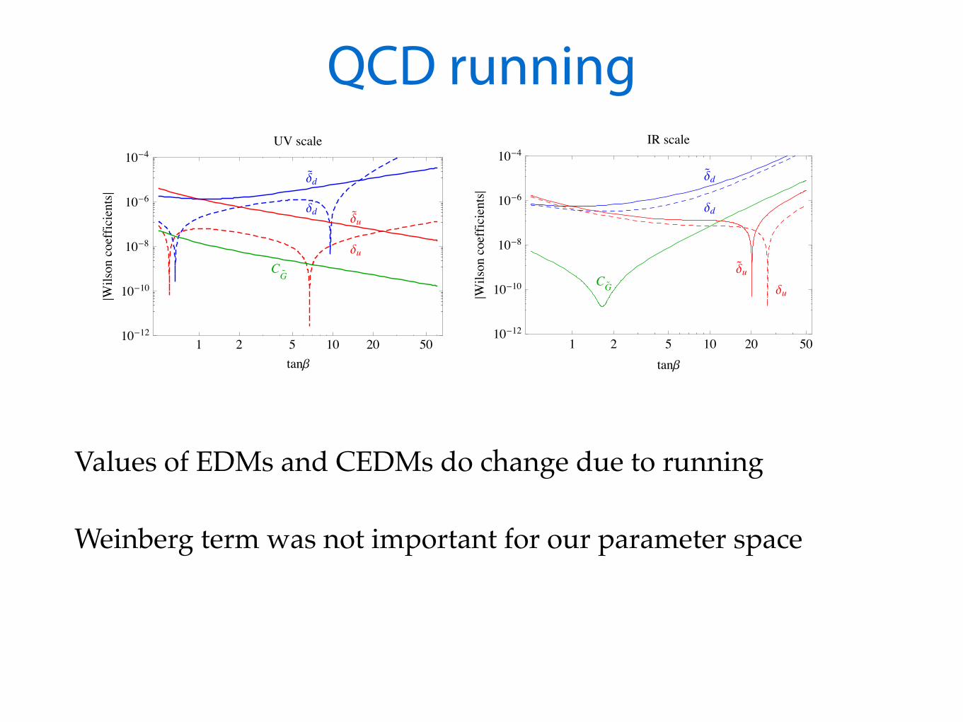
QCD running

Values of EDMs and CEDMs do change due to running

Weinberg term was not important for our parameter space

déu

du

dd

déd

CGé

1 2 5 10 20 5010-12

10-10

10-8

10-6

10-4

tanb

»Wilsoncoefficients»

UV scale

déu

du

dd

déd

CGé

1 2 5 10 20 5010-12

10-10

10-8

10-6

10-4

tanb

»Wilsoncoefficients»

IR scale

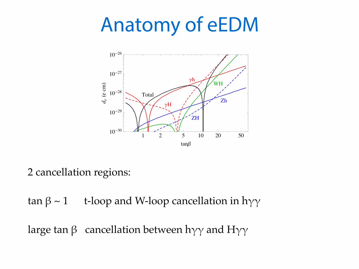
Anatomy of eEDM

2 cancellation regions:

tan β ~ 1 t-loop and W-loop cancellation in hγγ

large tan β cancellation between hγγ and Hγγ

Total

gH

WHgh

ZH

Zh

1 2 5 10 20 5010-30

10-29

10-28

10-27

10-26

tanb

d eHecm

L

Anatomy of eEDM

Not as intricate as eEDM

No cancellation regions (depends on choice of M.E.s)

Total EDM

CEDM

3G

1 2 5 10 20 5010-30

10-29

10-28

10-27

10-26

10-25

tanb

d nHecm

L

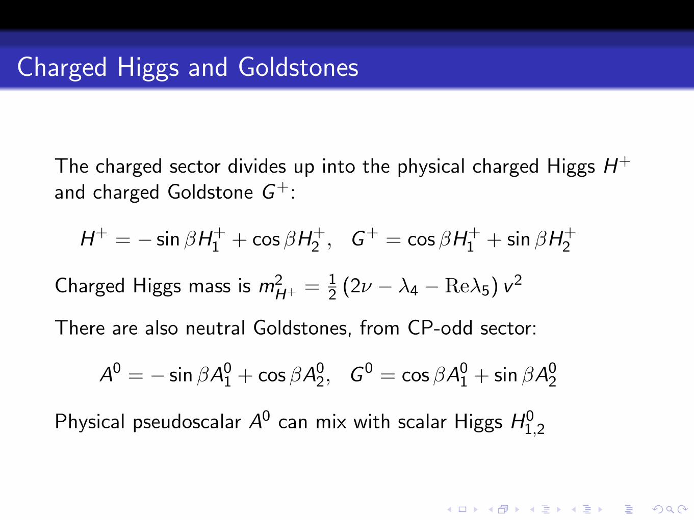
Charged Higgs and Goldstones

The charged sector divides up into the physical charged Higgs H+

and charged Goldstone G+:

H+ = � sin�H+1 + cos�H+

2 , G+ = cos�H+1 + sin�H+

2

Charged Higgs mass is m2H+ = 1

2 (2⌫ � �4 � Re�5) v2

There are also neutral Goldstones, from CP-odd sector:

A0 = � sin�A01 + cos�A0

2, G 0 = cos�A01 + sin�A0

2

Physical pseudoscalar A0 can mix with scalar Higgs H01,2

Fit to LHC Higgs data (type-I)

Fit to Higgs decay signal strengths (⇠ 25 fb�1)�� WW ZZ Vbb ⌧⌧

ATLAS 1.6± 0.3 1.0± 0.3 1.5± 0.4 �0.4± 1.0 0.8± 0.7CMS 0.8± 0.3 0.8± 0.2 0.9± 0.2 1.3± 0.6 1.1± 0.4

SM

-1.5-1.0-0.5 0.0 0.5 1.0 1.5-1.0

-0.5

0.0

0.5

1.0

a

a b

Combined, tan b=0.6

SM

-1.5-1.0-0.5 0.0 0.5 1.0 1.5-1.0

-0.5

0.0

0.5

1.0

a

Combined, tan b=1

SM

-1.5-1.0-0.5 0.0 0.5 1.0 1.5-1.0

-0.5

0.0

0.5

1.0

a

Combined, tan b=5

↵ mostly constrained near SM value (� � ⇡/2)↵b not well constrained

EDM current bounds (type-I)

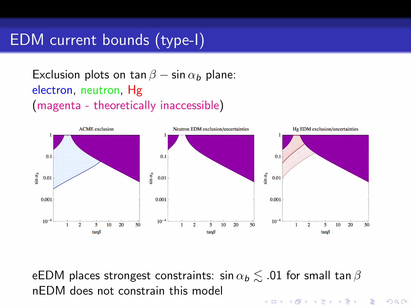
Exclusion plots on tan� � sin↵b plane:electron, neutron, Hg(magenta - theoretically inaccessible)

eEDM places strongest constraints: sin↵b . .01 for small tan�nEDM does not constrain this model

EDM future bounds (type-I)

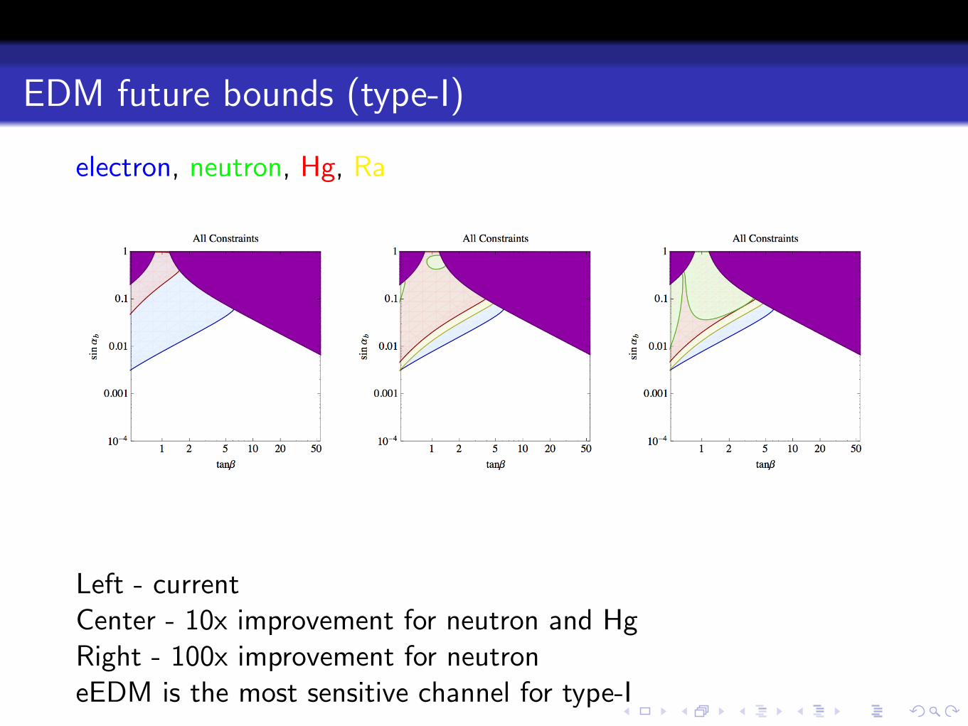
electron, neutron, Hg, Ra

Left - currentCenter - 10x improvement for neutron and HgRight - 100x improvement for neutroneEDM is the most sensitive channel for type-I