course file - geethanjali group of institutions · condensation: film wise and drop wise...
TRANSCRIPT

HEAT TRANSFER
COURSE FILE
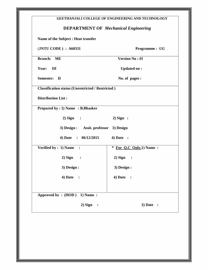
GEETHANJALI COLLEGE OF ENGINEERING AND TECHNOLOGY
DEPARTMENT OF Mechanical Engineering
Name of the Subject : Heat transfer
(JNTU CODE ) : A60331 Programme : UG
Branch: ME Version No : 01
Year: III Updated on :
Semester: II No. of pages :
Classification status (Unrestricted / Restricted )
Distribution List :
Prepared by : 1) Name : B.Bhasker
2) Sign : 2) Sign :
3) Design : Assit. professor 3) Design
4) Date : 06/12/2015 4) Date :
Verified by : 1) Name :
2) Sign :
3) Design :
4) Date :
* For Q.C Only.1) Name :
2) Sign :
3) Design :
4) Date :
Approved by : (HOD ) 1) Name :
2) Sign : 3) Date :
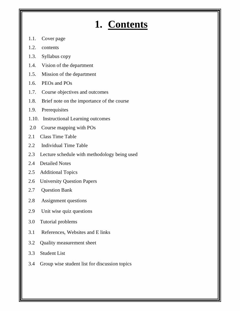
1. Contents 1.1. Cover page
1.2. contents
1.3. Syllabus copy
1.4. Vision of the department
1.5. Mission of the department
1.6. PEOs and POs
1.7. Course objectives and outcomes
1.8. Brief note on the importance of the course
1.9. Prerequisites
1.10. Instructional Learning outcomes
2.0 Course mapping with POs
2.1 Class Time Table
2.2 Individual Time Table
2.3 Lecture schedule with methodology being used
2.4 Detailed Notes
2.5 Additional Topics
2.6 University Question Papers
2.7 Question Bank
2.8 Assignment questions
2.9 Unit wise quiz questions
3.0 Tutorial problems
3.1 References, Websites and E links
3.2 Quality measurement sheet
3.3 Student List
3.4 Group wise student list for discussion topics
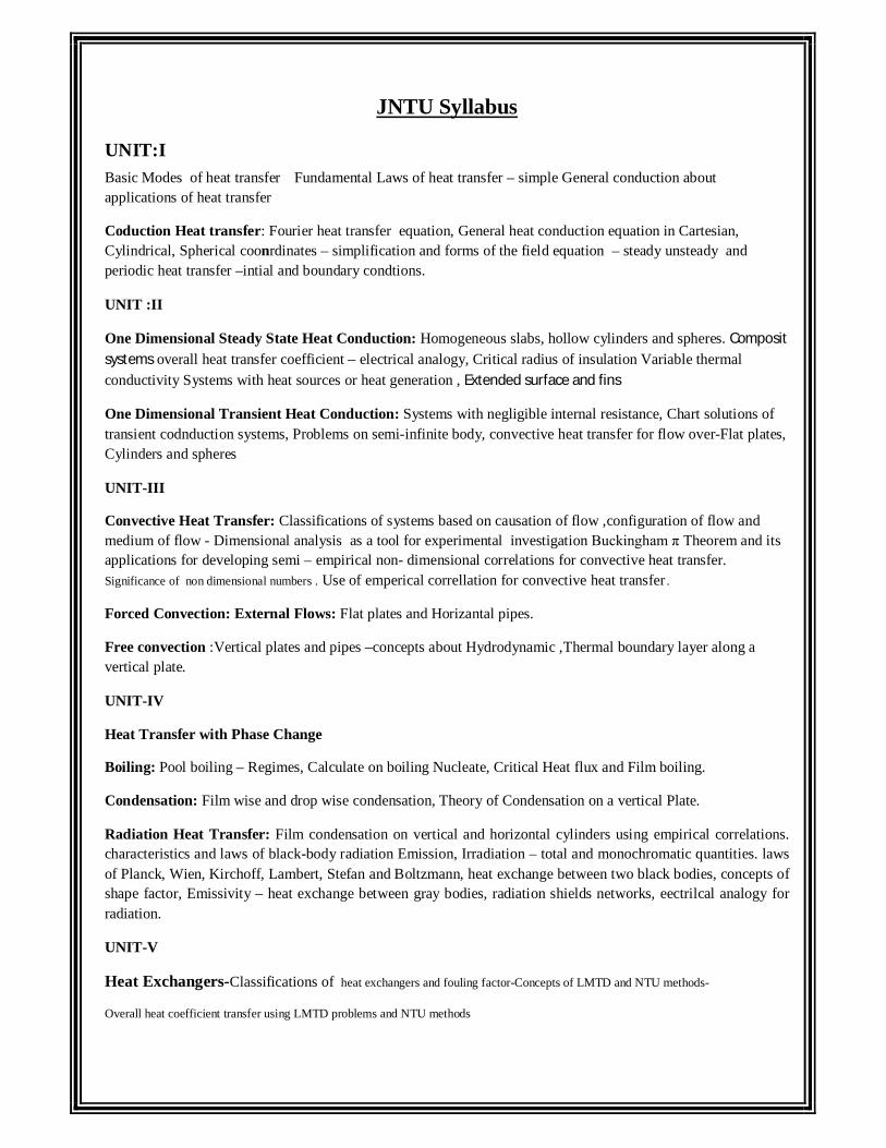
JNTU Syllabus
UNIT:I Basic Modes of heat transfer Fundamental Laws of heat transfer – simple General conduction about applications of heat transfer
Coduction Heat transfer: Fourier heat transfer equation, General heat conduction equation in Cartesian, Cylindrical, Spherical coonrdinates – simplification and forms of the field equation – steady unsteady and periodic heat transfer –intial and boundary condtions.
UNIT :II
One Dimensional Steady State Heat Conduction: Homogeneous slabs, hollow cylinders and spheres. Composit systems overall heat transfer coefficient – electrical analogy, Critical radius of insulation Variable thermal conductivity Systems with heat sources or heat generation , Extended surface and fins
One Dimensional Transient Heat Conduction: Systems with negligible internal resistance, Chart solutions of transient codnduction systems, Problems on semi-infinite body, convective heat transfer for flow over-Flat plates, Cylinders and spheres
UNIT-III
Convective Heat Transfer: Classifications of systems based on causation of flow ,configuration of flow and medium of flow - Dimensional analysis as a tool for experimental investigation Buckingham π Theorem and its applications for developing semi – empirical non- dimensional correlations for convective heat transfer. Significance of non dimensional numbers . Use of emperical correllation for convective heat transfer .
Forced Convection: External Flows: Flat plates and Horizantal pipes.
Free convection :Vertical plates and pipes –concepts about Hydrodynamic ,Thermal boundary layer along a vertical plate.
UNIT-IV
Heat Transfer with Phase Change
Boiling: Pool boiling – Regimes, Calculate on boiling Nucleate, Critical Heat flux and Film boiling.
Condensation: Film wise and drop wise condensation, Theory of Condensation on a vertical Plate.
Radiation Heat Transfer: Film condensation on vertical and horizontal cylinders using empirical correlations. characteristics and laws of black-body radiation Emission, Irradiation – total and monochromatic quantities. laws of Planck, Wien, Kirchoff, Lambert, Stefan and Boltzmann, heat exchange between two black bodies, concepts of shape factor, Emissivity – heat exchange between gray bodies, radiation shields networks, eectrilcal analogy for radiation.
UNIT-V
Heat Exchangers-Classifications of heat exchangers and fouling factor-Concepts of LMTD and NTU methods-
Overall heat coefficient transfer using LMTD problems and NTU methods

1.3 Vision of the Department:
To develop a world class program with excellence in teaching, learning and research
that would lead to growth, innovation and recognition
1.4 Mission of the Department:
The mission of the Mechanical Engineering Program is to benefit the society at large
by providing technical education to interested and capable students. These technocrats
should be able to apply basic and contemporary science, engineering and research
skills to identify problems in the industry and academia and be able to develop
practical solutions to them
1.5 PEOs and PO’s:
The Mechanical Engineering Department is dedicated to graduating mechanical engineers who:
Practice mechanical engineering in the general stems of thermal/fluid systems, mechanical
systems and design, and materials and manufacturing in industry and government settings.
Apply their engineering knowledge, critical thinking and problem solving skills in professional
engineering practice or in non-engineering fields, such as law, medicine or business.
Continue their intellectual development, through, for example, graduate education or professional
development courses.
Pursue advanced education, research and development, and other creative efforts in science and
technology.
Conduct them in a responsible, professional and ethical manner.
Participate as leaders in activities that support service to and economic development of the
region, state and nation.
1.6 Brief note on the importance of the cou
Course Goals
To learn basic principles and skills of modes of heat transfer
To learn the theory and characteristics of thermodynamics.
To learn and apply modes of heat transfer problems.
To develop the knowledge and skills needed to effectively evaluate heat transfer performed by others. *

Student Learning Objectives
Upon successful completion of this course, the student should be able to:
Objectives: The objective of this subject is to provide knowledge of modes of heat transfer.
Instructional learning out Comes
Students will learn advanced topics and techniques in completion of the course,after students will be able to: 1. Understand heat transfer through various modes. 2. Understand how heat and energy is transferred between the elements of a system for different
configurations, 3. Solve problems involving one or more modes of heat transfer Mapping on to Programme Educational Objectives and Programme Out Comes:
Relationship of the course to Programme out comes:
a Graduates will demonstrate knowledge of mathematics, science and engineering applications
√
b Graduates will demonstrate ability to identify, formulate and solve engineering problems
c Graduates will demonstrate an ability to analyze, design, develop and execute the programs efficiently and effectively
d Graduates will demonstrate an ability to design a system, software products and components as per requirements and specifications
e Graduates will demonstrate an ability to visualize and work on laboratories in multi-disciplinary tasks like microprocessors and interfacing, electronic devices and circuits etc.
f Graduates will demonstrate working in groups and possess project management skills to develop software projects.
g Graduates will demonstrate knowledge of professional and ethical responsibilities
h Graduates will be able to communicate effectively in both verbal and written
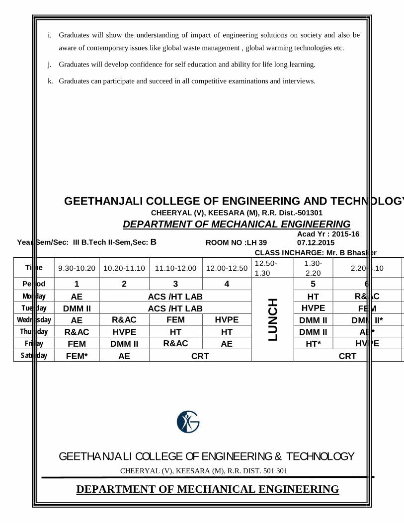
i Graduates will show the understanding of impact of engineering solutions on society and also be aware of contemporary issues like global waste management, global warming technologies etc.
j Graduates will develop confidence for self education and ability for life long learning.
k Graduates can participate and succeed in all competitive examinations and interviews.
Relationship of the course to the program educational objectives :
PEO 1 Our graduates will apply their knowledge and skills to succeed in a computer engineering career and/or obtain an advanced degree.

PEO 2 Our graduates will apply basic principles and practices of computing grounded in mathematics and science to successfully complete hardware and/or software related engineering projects to meet customer business objectives and/or productively engage in research.
√
PEO 3 Our graduates will function ethically and responsibly and will remain informed and involved as fully in their profession and in our society.
√
PEO 4 Our graduates will successfully function in multi-disciplinary teams.
PEO 5 Our graduates will communicate effectively both orally and in writing.
Program Educational Objectives:
PEO1: Our graduates will apply their knowledge and skills to succeed in a computer engineering
career and/or obtain an advanced degree.
PEO2: Our graduates will apply basic principles and practices of computing grounded in
mathematics and science to successfully complete hardware and/or software related engineering projects
to meet customer business objectives and/or productively engage in research.
PEO3: Our graduates will function ethically and responsibly and will remain informed and involved
as fully in their profession and in our society.
PEO4: Our graduates will successfully function in multi-disciplinary teams.
PEO5: Our graduates will communicate effectively both orally and in writing.
Outcomes:
a. Graduates will demonstrate knowledge of mathematics, science and engineering applications
b. Graduates will demonstrate ability to identify, formulate and solve engineering problems
c. Graduates will demonstrate an ability to analyse, design, develop and execute the programs
efficiently and effectively
d. Graduates will demonstrate an ability to design a system, software products and components as per
requirements and specifications
e. Graduates will demonstrate an ability to visualize and work on laboratories in multi-disciplinary
tasks like microprocessors and interfacing, electronic devices and circuits etc.
f. Graduates will demonstrate working in groups and possess project management skills to develop
software projects.
g. Graduates will demonstrate knowledge of professional and ethical responsibilities
h. Graduates will be able to communicate effectively in both verbal and written
i. Graduates will show the understanding of impact of engineering solutions on society and also be
aware of contemporary issues like global waste management , global warming technologies etc.
j. Graduates will develop confidence for self education and ability for life long learning.
k. Graduates can participate and succeed in all competitive examinations and interviews.
GEETHANJALI COLLEGE OF ENGINEERING & TECHNOLOGY CHEERYAL (V), KEESARA (M), R.R. DIST. 501 301
DEPARTMENT OF MECHANICAL ENGINEERING
GEETHANJALI COLLEGE OF ENGINEERING AND TECHNOLOGYCHEERYAL (V), KEESARA (M), R.R. Dist.-501301
DEPARTMENT OF MECHANICAL ENGINEERING Year/Sem/Sec: III B.Tech II-Sem,Sec: B ROOM NO :LH 39
Acad Yr : 2015-16 WEF: 07.12.2015
CLASS INCHARGE: Mr. B Bhasker
Time 9.30-10.20 10.20-11.10 11.10-12.00 12.00-12.50 12.50-1.30
1.30-2.20
2.20-3.10
Period 1 2 3 4 LU
NC
H
5 6
Monday AE ACS /HT LAB HT R&AC Tuesday DMM II ACS /HT LAB HVPE FEM
Wednesday AE R&AC FEM HVPE DMM II DMM II* Thursday R&AC HVPE HT HT DMM II AE*
Friday FEM DMM II R&AC AE HT* HVPE Saturday FEM* AE CRT CRT
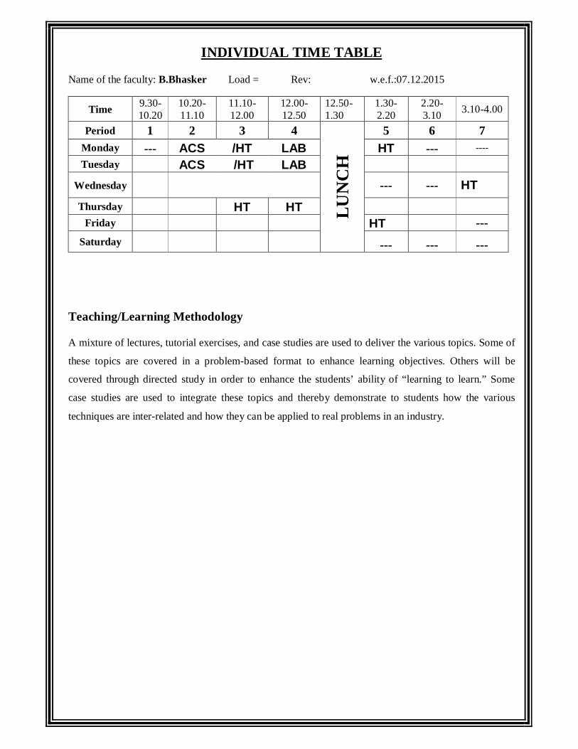
INDIVIDUAL TIME TABLE
Name of the faculty: B.Bhasker Load = Rev: w.e.f.:07.12.2015
Time 9.30-10.20
10.20-11.10
11.10-12.00
12.00-12.50
12.50-1.30
1.30-2.20
2.20-3.10 3.10-4.00
Period 1 2 3 4
LUN
CH
5 6 7 Monday --- ACS /HT LAB HT --- ----
Tuesday ACS /HT LAB Wednesday --- --- HT
Thursday HT HT Friday HT ---
Saturday --- --- ---
Teaching/Learning Methodology
A mixture of lectures, tutorial exercises, and case studies are used to deliver the various topics. Some of
these topics are covered in a problem-based format to enhance learning objectives. Others will be
covered through directed study in order to enhance the students’ ability of “learning to learn.” Some
case studies are used to integrate these topics and thereby demonstrate to students how the various
techniques are inter-related and how they can be applied to real problems in an industry.

S.No
Unit No.
Total No. of classes
Date Topic to be covered in One Lecture Reg/ Additional
Teaching aids used PPT/BB
1
I
2
Basic Modes of heat transfer Regular BB
2 2
Fundamental Laws of heat transfer – simple General conduction about applications of heat transfer
Regular BB
3 1
Conduction Heat transfer: Fourier heat transfer equation Regular BB
4 1 General heat conduction equation in Cartesian Regular BB
5 3
Cylindrical, Spherical coordinates – Regular BB
6 2
simplification and forms of the field equation – steady unsteady and periodic heat transfer –intial and boundary condtions BB
8
II
1
One Dimensional Steady State Heat Conduction Regular PPT
9 1
Homogeneous slabs, hollow cylinders
and spheres Regular PPT
10 1
Composit systems Regular PPT
11 1
overall heat transfer coefficient – electrical analogy Regular BB
12 1 Critical radius of insulation Regular BB 13 1 Variable thermal conductivity BB
14 2
Systems with heat sources or heat generation , Extended surface and fins Regular BB
15 1
One Dimensional Transient Heat Conduction
Regular BB
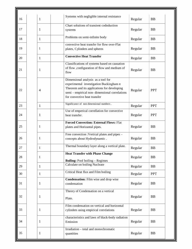
16 1
Systems with negligible internal resistance Regular BB
17 1
Chart solutions of transient codnduction systems Regular BB
18 1 Problems on semi-infinite body Regular BB
19 1
convective heat transfer for flow over-Flat plates, Cylinders and spheres Regular BB
20 1 Convective Heat Transfer Regular BB
21 1
Classifications of systems based on causation of flow ,configuration of flow and medium of flow
Regular BB
22 4
Dimensional analysis as a tool for experimental investigation Buckingham π Theorem and its applications for developing semi – empirical non- dimensional correlations for convective heat transfer
Regular PPT
23 1 Significance of non dimensional numbers . Regular PPT
24 1
Use of emperical correllation for convective heat transfer . Regular PPT
25 1
Forced Convection: External Flows: Flat plates and Horizantal pipes. Regular BB
26 1
Free convection :Vertical plates and pipes –concepts about Hydrodynamic . Regular BB
27 1 Thermal boundary layer along a vertical plate. Regular BB
28 1
Heat Transfer with Phase Change
Boiling: Pool boiling – Regimes Regular BB
29 1 Calculate on boiling Nucleate Regular BB
30 1 Critical Heat flux and Film boiling Regular PPT
31 1
Condensation: Film wise and drop wise condensation Regular BB
32 1
Theory of Condensation on a vertical
Plate. Regular BB
33 1 Film condensation on vertical and horizontal cylinders using empirical correlations Regular BB
34 1
characteristics and laws of black-body radiation Emission Regular BB
35 1
Irradiation – total and monochromatic quantities Regular BB
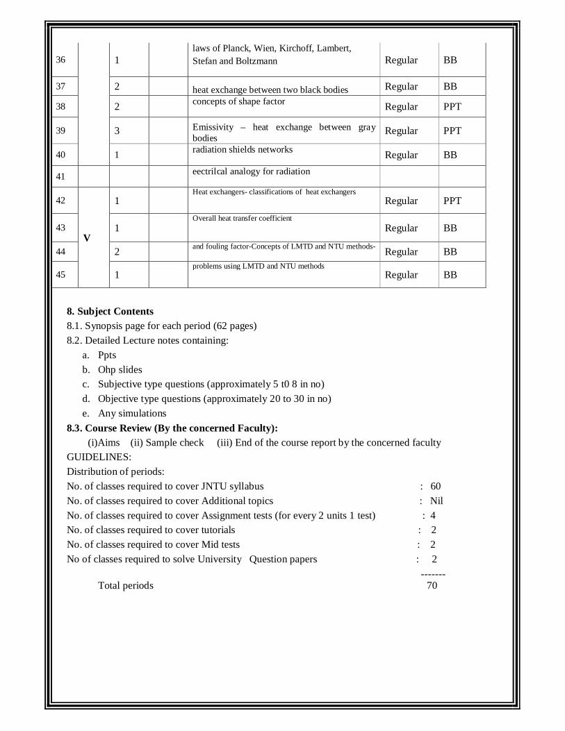
36 1
laws of Planck, Wien, Kirchoff, Lambert, Stefan and Boltzmann Regular BB
37 2 heat exchange between two black bodies Regular BB
38 2 concepts of shape factor Regular PPT
39 3
Emissivity – heat exchange between gray bodies
Regular PPT
40 1 radiation shields networks Regular BB
41 eectrilcal analogy for radiation
42
V
1
Heat exchangers- classifications of heat exchangers Regular PPT
43 1
Overall heat transfer coefficient Regular BB
44 2 and fouling factor-Concepts of LMTD and NTU methods- Regular BB
45 1
problems using LMTD and NTU methods Regular BB
8. Subject Contents 8.1. Synopsis page for each period (62 pages) 8.2. Detailed Lecture notes containing:
a. Ppts b. Ohp slides c. Subjective type questions (approximately 5 t0 8 in no) d. Objective type questions (approximately 20 to 30 in no) e. Any simulations
8.3. Course Review (By the concerned Faculty): (i)Aims (ii) Sample check (iii) End of the course report by the concerned faculty GUIDELINES: Distribution of periods: No. of classes required to cover JNTU syllabus : 60 No. of classes required to cover Additional topics : Nil No. of classes required to cover Assignment tests (for every 2 units 1 test) : 4 No. of classes required to cover tutorials : 2 No. of classes required to cover Mid tests : 2 No of classes required to solve University Question papers : 2
------- Total periods 70

TUTORIAL CLASS TOPICS
S.
No. Tutorial class Topic Regular /
Additional Teaching aids used
LCD/OHP/BB Date Rem
arks
1
2
3
4
5
6
7
9
10
11
12
13
14
15
16
17
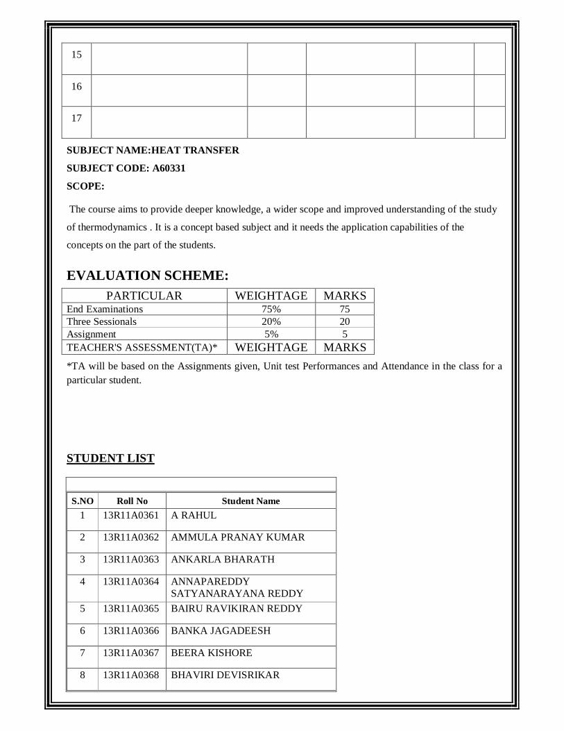
SUBJECT NAME:HEAT TRANSFER
SUBJECT CODE: A60331
SCOPE:
The course aims to provide deeper knowledge, a wider scope and improved understanding of the study
of thermodynamics . It is a concept based subject and it needs the application capabilities of the
concepts on the part of the students.
EVALUATION SCHEME: PARTICULAR WEIGHTAGE MARKS
End Examinations 75% 75 Three Sessionals 20% 20 Assignment 5% 5 TEACHER'S ASSESSMENT(TA)* WEIGHTAGE MARKS *TA will be based on the Assignments given, Unit test Performances and Attendance in the class for a particular student.
STUDENT LIST
S.NO Roll No Student Name 1 13R11A0361 A RAHUL
2 13R11A0362 AMMULA PRANAY KUMAR
3 13R11A0363 ANKARLA BHARATH
4 13R11A0364 ANNAPAREDDY SATYANARAYANA REDDY
5 13R11A0365 BAIRU RAVIKIRAN REDDY
6 13R11A0366 BANKA JAGADEESH
7 13R11A0367 BEERA KISHORE
8 13R11A0368 BHAVIRI DEVISRIKAR
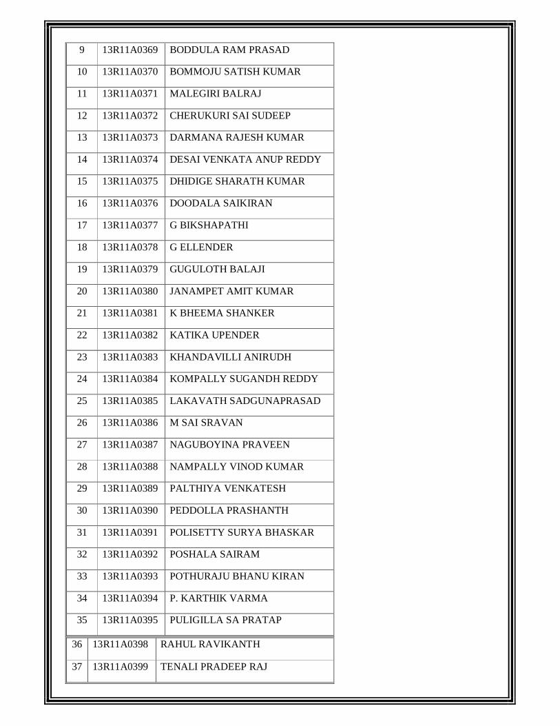
9 13R11A0369 BODDULA RAM PRASAD
10 13R11A0370 BOMMOJU SATISH KUMAR
11 13R11A0371 MALEGIRI BALRAJ
12 13R11A0372 CHERUKURI SAI SUDEEP
13 13R11A0373 DARMANA RAJESH KUMAR
14 13R11A0374 DESAI VENKATA ANUP REDDY
15 13R11A0375 DHIDIGE SHARATH KUMAR
16 13R11A0376 DOODALA SAIKIRAN
17 13R11A0377 G BIKSHAPATHI
18 13R11A0378 G ELLENDER
19 13R11A0379 GUGULOTH BALAJI
20 13R11A0380 JANAMPET AMIT KUMAR
21 13R11A0381 K BHEEMA SHANKER
22 13R11A0382 KATIKA UPENDER
23 13R11A0383 KHANDAVILLI ANIRUDH
24 13R11A0384 KOMPALLY SUGANDH REDDY
25 13R11A0385 LAKAVATH SADGUNAPRASAD
26 13R11A0386 M SAI SRAVAN
27 13R11A0387 NAGUBOYINA PRAVEEN
28 13R11A0388 NAMPALLY VINOD KUMAR
29 13R11A0389 PALTHIYA VENKATESH
30 13R11A0390 PEDDOLLA PRASHANTH
31 13R11A0391 POLISETTY SURYA BHASKAR
32 13R11A0392 POSHALA SAIRAM
33 13R11A0393 POTHURAJU BHANU KIRAN
34 13R11A0394 P. KARTHIK VARMA
35 13R11A0395 PULIGILLA SA PRATAP
36 13R11A0398 RAHUL RAVIKANTH
37 13R11A0399 TENALI PRADEEP RAJ
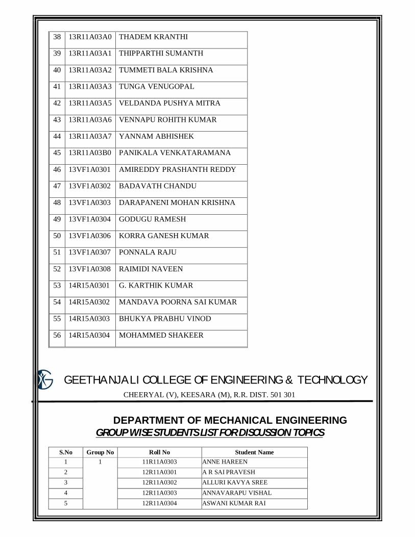
38 13R11A03A0 THADEM KRANTHI
39 13R11A03A1 THIPPARTHI SUMANTH
40 13R11A03A2 TUMMETI BALA KRISHNA
41 13R11A03A3 TUNGA VENUGOPAL
42 13R11A03A5 VELDANDA PUSHYA MITRA
43 13R11A03A6 VENNAPU ROHITH KUMAR
44 13R11A03A7 YANNAM ABHISHEK
45 13R11A03B0 PANIKALA VENKATARAMANA
46 13VF1A0301 AMIREDDY PRASHANTH REDDY
47 13VF1A0302 BADAVATH CHANDU
48 13VF1A0303 DARAPANENI MOHAN KRISHNA
49 13VF1A0304 GODUGU RAMESH
50 13VF1A0306 KORRA GANESH KUMAR
51 13VF1A0307 PONNALA RAJU
52 13VF1A0308 RAIMIDI NAVEEN
53 14R15A0301 G. KARTHIK KUMAR
54 14R15A0302 MANDAVA POORNA SAI KUMAR
55 14R15A0303 BHUKYA PRABHU VINOD
56 14R15A0304 MOHAMMED SHAKEER
GEETHANJALI COLLEGE OF ENGINEERING & TECHNOLOGY
CHEERYAL (V), KEESARA (M), R.R. DIST. 501 301
DEPARTMENT OF MECHANICAL ENGINEERING
GROUP WISE STUDENTS LIST FOR DISCUSSION TOPICS
S.No Group No Roll No Student Name 1 1 11R11A0303 ANNE HAREEN 2 12R11A0301 A R SAI PRAVESH 3 12R11A0302 ALLURI KAVYA SREE 4 12R11A0303 ANNAVARAPU VISHAL 5 12R11A0304 ASWANI KUMAR RAI
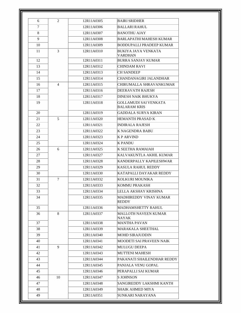
6 2 12R11A0305 BAIRI SRIDHER 7 12R11A0306 BALLARI RAHUL 8 12R11A0307 BANOTHU AJAY 9 12R11A0308 BARLAPATHI MAHESH KUMAR
10 12R11A0309 BODDUPALLI PRADEEP KUMAR 11 3 12R11A0310 BUKIYA JAYA VENKATA
VARDHAN 12 12R11A0311 BURRA SANJAY KUMAR 13 12R11A0312 CHINDAM RAVI 14 12R11A0313 CH SANDEEP 15 12R11A0314 CHANDANAGIRI JALANDHAR 16 4 12R11A0315 CHIRUMALLA SHRAVANKUMAR 17 12R11A0316 DEERAVATH RAJESH 18 12R11A0317 DINESH NAIK BHUKYA 19 12R11A0318 GOLLAMUDI SAI VENKATA
BALARAM KRIS 20 12R11A0319 GADDALA SURYA KIRAN 21 5 12R11A0320 HEMANTH PRASAD K 22 12R11A0321 INDIRALA RAJESH 23 12R11A0322 K NAGENDRA BABU 24 12R11A0323 K P ARVIND 25 12R11A0324 K PANDU 26 6 12R11A0325 K SEETHA RAMAIAH 27 12R11A0327 KALVAKUNTLA AKHIL KUMAR 28 12R11A0328 KANDERPALLY KAPILESHWAR 29 12R11A0329 KASULA RAHUL REDDY 30 12R11A0330 KATAPALLI DAYAKAR REDDY 31 7 12R11A0332 KOLKURI MOUNIKA 32 12R11A0333 KOMMU PRAKASH 33 12R11A0334 LELLA AKSHAY KRISHNA 34 12R11A0335 MADHIREDDY VINAY KUMAR
REDDY 35 12R11A0336 MADHAMSHETTY RAHUL 36 8 12R11A0337 MALLOTH NAVEEN KUMAR
NAYAK 37 12R11A0338 MANTHA PAVAN 38 12R11A0339 MARAKALA SHEETHAL 39 12R11A0340 MOHD SIRAJUDDIN 40 12R11A0341 MOODETI SAI PRAVEEN NAIK 41 9 12R11A0342 MULUGU DEEPA 42 12R11A0343 MUTTENI MAHESH 43 12R11A0344 PAKANATI SHAILENDHAR REDDY 44 12R11A0345 PANJALA VENU GOPAL 45 12R11A0346 PERAPALLI SAI KUMAR 46 10 12R11A0347 S JOHNSON 47 12R11A0348 SANGIREDDY LAKSHMI KANTH 48 12R11A0349 SHAIK AHMED MIYA 49 12R11A0351 SUNKARI NARAYANA
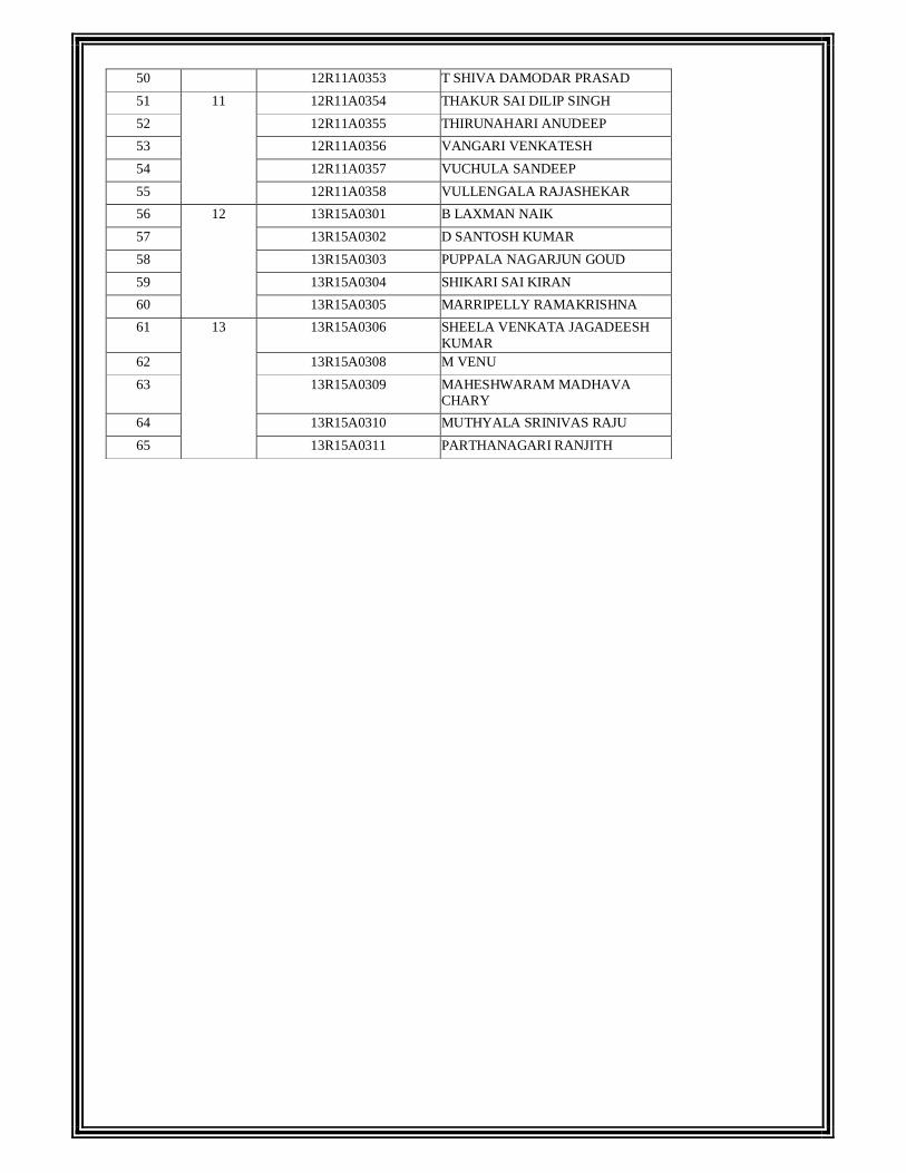
50 12R11A0353 T SHIVA DAMODAR PRASAD 51 11 12R11A0354 THAKUR SAI DILIP SINGH 52 12R11A0355 THIRUNAHARI ANUDEEP 53 12R11A0356 VANGARI VENKATESH 54 12R11A0357 VUCHULA SANDEEP 55 12R11A0358 VULLENGALA RAJASHEKAR 56 12 13R15A0301 B LAXMAN NAIK 57 13R15A0302 D SANTOSH KUMAR 58 13R15A0303 PUPPALA NAGARJUN GOUD 59 13R15A0304 SHIKARI SAI KIRAN 60 13R15A0305 MARRIPELLY RAMAKRISHNA 61 13 13R15A0306 SHEELA VENKATA JAGADEESH
KUMAR 62 13R15A0308 M VENU 63 13R15A0309 MAHESHWARAM MADHAVA
CHARY 64 13R15A0310 MUTHYALA SRINIVAS RAJU 65 13R15A0311 PARTHANAGARI RANJITH
UNIT – I
BASIC CONCEPTS IN HEAT TRANSFER
1.1 Heat Energy and Heat Transfer
Heat is a form of energy in transition and it flows from one system to another, without transfer
of mass, whenever there is a temperature difference between the systems. The process of heat transfer
means the exchange in internal energy between the systems and in almost every phase of scientific and
engineering work processes, we encounter the flow of heat energy.
1.2 Importance of Heat Transfer
Heat transfer processes involve the transfer and conversion of energy and therefore, it is
essential to determine the specified rate of heat transfer at a specified temperature difference. The design
of equipments like boilers, refrigerators and other heat exchangers require a detailed analysis of
transferring a given amount of heat energy within a specified time. Components like gas/steam turbine
blades, combustion chamber walls, electrical machines, electronic gadgets, transformers, bearings, etc
require continuous removal of heat energy at a rapid rate in order to avoid their overheating. Thus, a
thorough understanding of the physical mechanism of heat flow and the governing laws of heat transfer
are a must.
1.3 Modes of Heat Transfer
The heat transfer processes have been categorized into three basic modes: Conduction,
Convection and Radiation.
Conduction – It is the energy transfer from the more energetic to the less energetic particles of a
substance due to interaction between them, a microscopic activity.
Convection - It is the energy transfer due to random molecular motion a long with the macroscopic
motion of the fluid particles.
Radiation - It is the energy emitted by matter which is at finite temperature. All forms of matter emit
radiation attributed to changes m the electron configuration of the constituent atoms or
molecules The transfer of energy by conduction and convection requires the presence of
a material medium whereas radiation does not. In fact radiation transfer is most efficient
in vacuum.
All practical problems of importance encountered in our daily life Involve at least two, and
sometimes all the three modes occuring simultaneously When the rate of heat flow is constant, i.e., does
not vary with time, the process is called a steady state heat transfer process. When the temperature at
any point in a system changes with time, the process is called unsteady or transient process. The internal
energy of the system changes in such a process when the temperature variation of an unsteady process
describes a particular cycle (heating or cooling of a budding wall during a 24 hour cycle), the process is
called a periodic or quasi-steady heat transfer process.
Heat transfer may take place when there is a difference In the concentration of the mixture
components (the diffusion thermoeffect). Many heat transfer processes are accompanied by a transfer of
mass on a macroscopic scale. We know that when water evaporates, the heal transfer is accompanied by
the transport of the vapour formed through an air-vapour mixture. The transport of heat energy to steam
generally occurs both through molecular interaction and convection. The combined molecular and
convective transport of mass is called convection mass transfer and with this mass transfer, the process
of heat transfer becomes more complicated.
1.4 Thermodynamics and Heat Transfer-Basic Difference
Thermodynamics is mainly concerned with the conversion of heat energy into other useful
forms of energy and IS based on (i) the concept of thermal equilibrium (Zeroth Law), (ii) the First Law
(the principle of conservation of energy) and (iii) the Second Law (the direction in which a particular
process can take place). Thermodynamics is silent about the heat energy exchange mechanism. The
transfer of heat energy between systems can only take place whenever there is a temperature gradient
and thus. Heat transfer is basically a non-equilibrium phenomenon. The Science of heat transfer tells us
the rate at which the heat energy can be transferred when there IS a thermal non-equilibrium. That IS,
the science of heat transfer seeks to do what thermodynamics is inherently unable to do.
However, the subjects of heat transfer and thermodynamics are highly complimentary. Many
heat transfer problems can be solved by applying the principles of conservation of energy (the First
Law)
1.5 Dimension and Unit
Dimensions and units are essential tools of engineering. Dimension is a set of basic entities
expressing the magnitude of our observations of certain quantities. The state of a system is identified by
its observable properties, such as mass, density, temperature, etc. Further, the motion of an object will
be affected by the observable properties of that medium in which the object is moving. Thus a number
of observable properties are to be measured to identify the state of the system.
A unit is a definite standard by which a dimension can be described. The difference between a
dimension and the unit is that a dimension is a measurable property of the system and the unit is the
standard element in terms of which a dimension can be explicitly described with specific numerical
values.
Every major country of the world has decided to use SI units. In the study of heat transfer the
dimensions are: L for length, M for mass, e for temperature, T for time and the corresponding units are:
metre for length, kilogram for mass, degree Celsius (oC) or Kelvin (K) for temperature and second (s)
for time. The parameters important In the study of heat transfer are tabulated in Table 1.1 with their
basic dimensions and units of measurement.
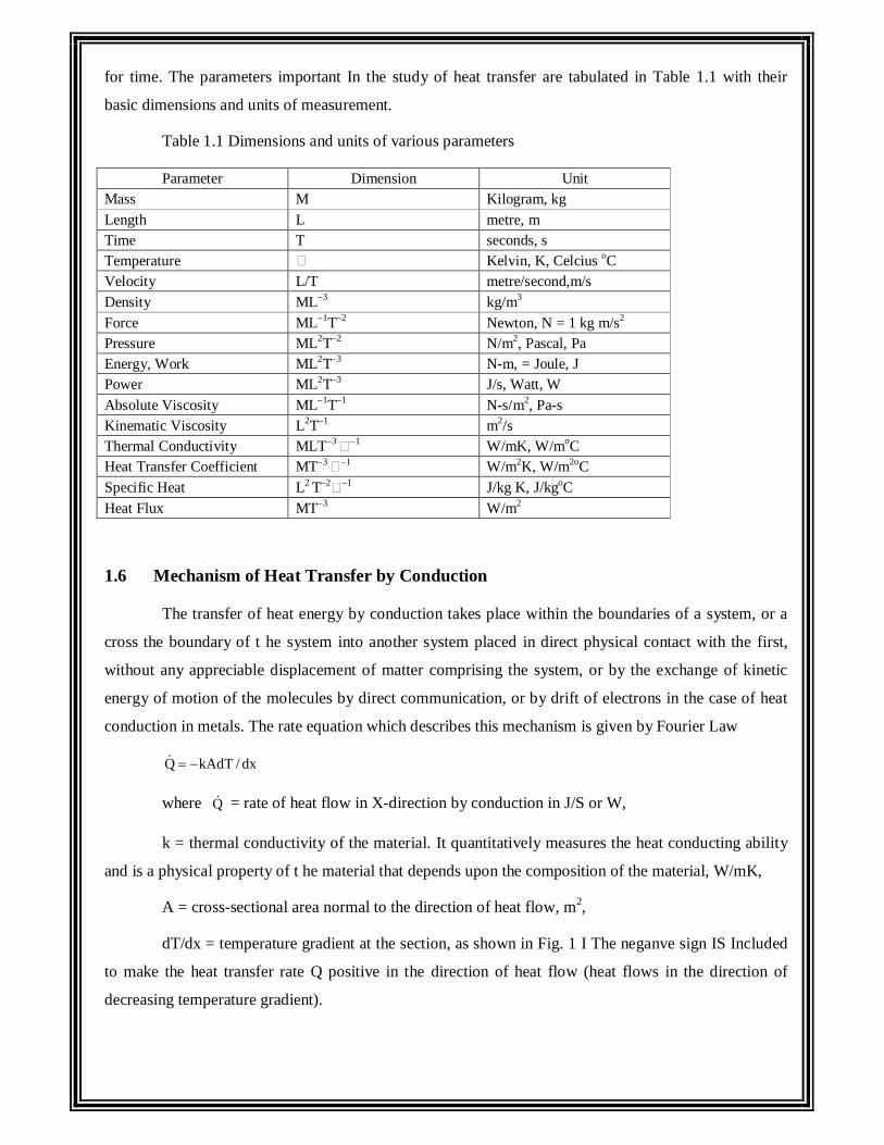
Table 1.1 Dimensions and units of various parameters
Parameter Dimension Unit Mass M Kilogram, kg Length L metre, m Time T seconds, s Temperature Kelvin, K, Celcius oC Velocity L/T metre/second,m/s Density ML–3 kg/m3 Force ML–1T–2 Newton, N = 1 kg m/s2 Pressure ML2T–2 N/m2, Pascal, Pa Energy, Work ML2T–3 N-m, = Joule, J Power ML2T–3 J/s, Watt, W Absolute Viscosity ML–1T–1 N-s/m2, Pa-s Kinematic Viscosity L2T–1 m2/s Thermal Conductivity MLT–3 –1 W/mK, W/moC Heat Transfer Coefficient MT–3 –1 W/m2K, W/m2oC Specific Heat L2 T–2 –1 J/kg K, J/kgoC Heat Flux MT–3 W/m2
1.6 Mechanism of Heat Transfer by Conduction
The transfer of heat energy by conduction takes place within the boundaries of a system, or a
cross the boundary of t he system into another system placed in direct physical contact with the first,
without any appreciable displacement of matter comprising the system, or by the exchange of kinetic
energy of motion of the molecules by direct communication, or by drift of electrons in the case of heat
conduction in metals. The rate equation which describes this mechanism is given by Fourier Law
Q kAdT / dx
where Q = rate of heat flow in X-direction by conduction in J/S or W,
k = thermal conductivity of the material. It quantitatively measures the heat conducting ability
and is a physical property of t he material that depends upon the composition of the material, W/mK,
A = cross-sectional area normal to the direction of heat flow, m2,
dT/dx = temperature gradient at the section, as shown in Fig. 1 I The neganve sign IS Included
to make the heat transfer rate Q positive in the direction of heat flow (heat flows in the direction of
decreasing temperature gradient).
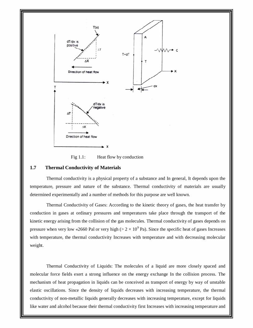
Fig 1.1: Heat flow by conduction
1.7 Thermal Conductivity of Materials
Thermal conductivity is a physical property of a substance and In general, It depends upon the
temperature, pressure and nature of the substance. Thermal conductivity of materials are usually
determined experimentally and a number of methods for this purpose are well known.
Thermal Conductivity of Gases: According to the kinetic theory of gases, the heat transfer by
conduction in gases at ordinary pressures and temperatures take place through the transport of the
kinetic energy arising from the collision of the gas molecules. Thermal conductivity of gases depends on
pressure when very low «2660 Pal or very high (> 2 × 10⁹ Pa). Since the specific heat of gases Increases
with temperature, the thermal conductivity Increases with temperature and with decreasing molecular
weight.
Thermal Conductivity of Liquids: The molecules of a liquid are more closely spaced and
molecular force fields exert a strong influence on the energy exchange In the collision process. The
mechanism of heat propagation in liquids can be conceived as transport of energy by way of unstable
elastic oscillations. Since the density of liquids decreases with increasing temperature, the thermal
conductivity of non-metallic liquids generally decreases with increasing temperature, except for liquids
like water and alcohol because their thermal conductivity first Increases with increasing temperature and
then decreases.
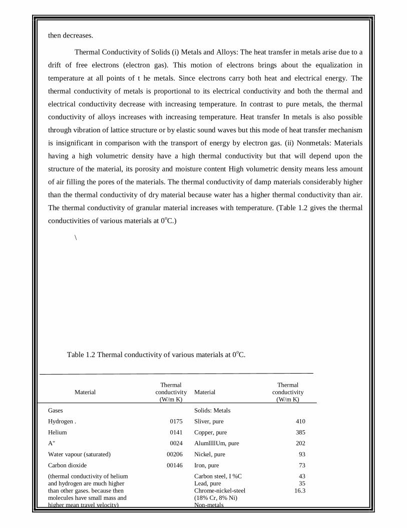
Thermal Conductivity of Solids (i) Metals and Alloys: The heat transfer in metals arise due to a
drift of free electrons (electron gas). This motion of electrons brings about the equalization in
temperature at all points of t he metals. Since electrons carry both heat and electrical energy. The
thermal conductivity of metals is proportional to its electrical conductivity and both the thermal and
electrical conductivity decrease with increasing temperature. In contrast to pure metals, the thermal
conductivity of alloys increases with increasing temperature. Heat transfer In metals is also possible
through vibration of lattice structure or by elastic sound waves but this mode of heat transfer mechanism
is insignificant in comparison with the transport of energy by electron gas. (ii) Nonmetals: Materials
having a high volumetric density have a high thermal conductivity but that will depend upon the
structure of the material, its porosity and moisture content High volumetric density means less amount
of air filling the pores of the materials. The thermal conductivity of damp materials considerably higher
than the thermal conductivity of dry material because water has a higher thermal conductivity than air.
The thermal conductivity of granular material increases with temperature. (Table 1.2 gives the thermal
conductivities of various materials at 0oC.)
\
Table 1.2 Thermal conductivity of various materials at 0oC.
Thermal Thermal Material conductivity Material conductivity (W/m K) (W/m K)
Gases Solids: Metals
Hydrogen . 0175 Sliver, pure 410
Helium 0141 Copper, pure 385
A" 0024 AlumllllUm, pure 202
Water vapour (saturated) 00206 Nickel, pure 93
Carbon dioxide 00146 Iron, pure 73
(thermal conductivity of helium Carbon steel, I %C 43 and hydrogen are much higher Lead, pure 35 than other gases. because then Chrome-nickel-steel 16.3 molecules have small mass and (18% Cr, 8% Ni) higher mean travel velocity) Non-metals
Liquids Quartz, parallel to axis 41.6
Mercury 821 Magnesite 4.15
Water* 0.556 Marble 2.08 to 2.94
Ammonia 0.54 Sandstone 1.83
Lubricating 011 Glass, window 0.78
SAE 40 0.147 Maple or Oak 0.17
Freon 12 0.073 Saw dust 0.059
Glass wool 0.038
* water has its maximum thermal conductivity (k = 068 W/mK) at about 150oC
2. STEADY STATE CONDUCTION ONE DIMENSION
2.1 The General Heat Conduction Equation for an Isotropic Solid with Constant
Thermal Conductivity
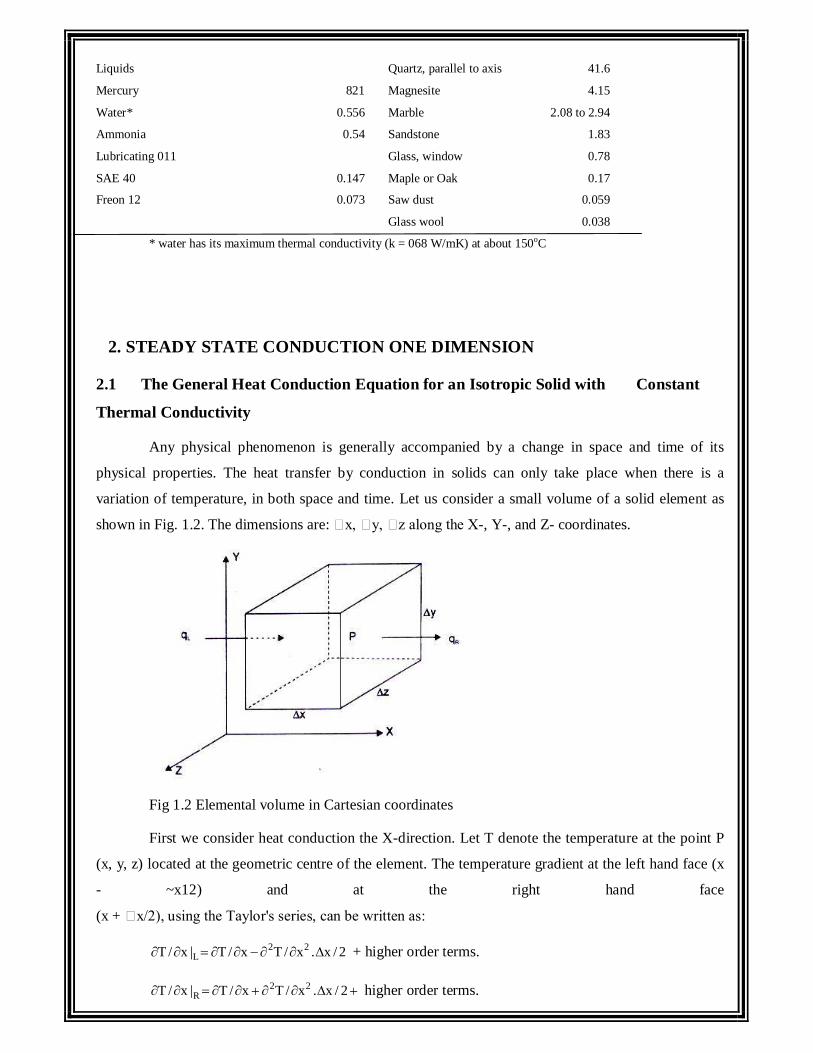
Any physical phenomenon is generally accompanied by a change in space and time of its
physical properties. The heat transfer by conduction in solids can only take place when there is a
variation of temperature, in both space and time. Let us consider a small volume of a solid element as
shown in Fig. 1.2. The dimensions are: x, y, z along the X-, Y-, and Z- coordinates.
Fig 1.2 Elemental volume in Cartesian coordinates
First we consider heat conduction the X-direction. Let T denote the temperature at the point P
(x, y, z) located at the geometric centre of the element. The temperature gradient at the left hand face (x
- ~x12) and at the right hand face
(x + x/2), using the Taylor's series, can be written as:
2 2LT / x | T / x T / x . x / 2 + higher order terms.
2 2RT / x | T / x T / x . x / 2 higher order terms.
The net rate at which heat is conducted out of the element 10 X-direction assuming k as
constant and neglecting the higher order terms,
we get 2 2
2 2T T x T T xk y zx 2 x 2x x
2
2Tk y z x
x
Similarly for Y- and Z-direction,
We have 2 2k x y z T / y and 2 2k x y z T / z .
If there is heat generation within the element as Q, per unit volume and the internal energy of
the element changes with time, by making an energy balance, we write
Heat generated within Heat conducted away Rate of change of internal
the element from the element energy within with the element
or, 2 2 2 2 2 2vQ x y z k x y z T / x T / y T / z
c x y z T / t
Upon simplification, 2 2 2 2 2 2v
cT / x T / y T / z Q / k T / tk
or, 2vT Q / k 1/ T / t
where k / . c , is called the thermal diffusivity and is seen to be a physical property of the
material of which the solid is composed.
The Eq. (2.la) is the general heat conduction equation for an isotropic solid with a constant
thermal conductivity. The equation in cylindrical (radius r, axis Z and longitude ) coordinates is
written as: Fig. 2.I(b),
2 2 2 2 2 2 2vT / r 1/ r T / r 1/ r T / T / z Q / k 1/ T / t (2.1b)
And, in spherical polar coordinates Fig. 2.1(c) (radius, longitude, colatitudes) is
22 v
2 2 2 2 2Q1 T 1 T 1 T 1 Tr sin
r r k tr r sin r sin
(2.1c)
Under steady state or stationary condition, the temperature of a body does not vary with time,
i.e. T / t 0 . And, with no internal generation, the equation (2.1) reduces to
2T 0
It should be noted that Fourier law can always be used to compute the rate of heat transfer by
conduction from the knowledge of temperature distribution even for unsteady condition and with
internal heat generation.
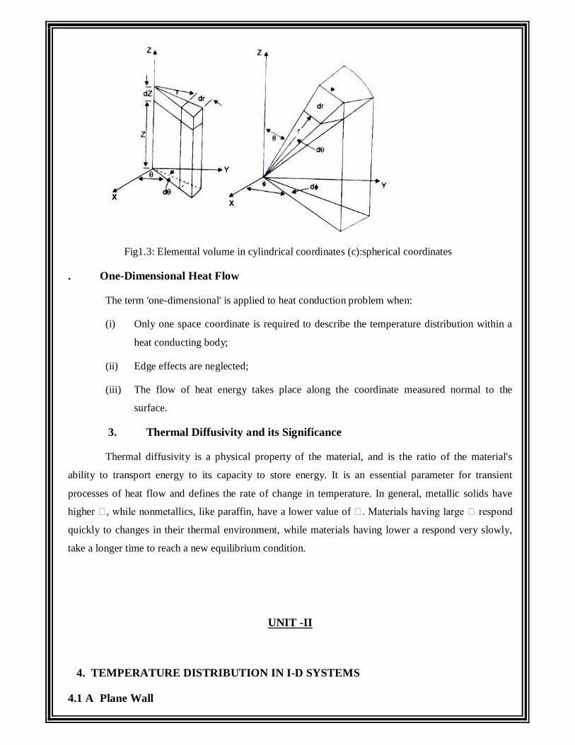
Fig1.3: Elemental volume in cylindrical coordinates (c):spherical coordinates
. One-Dimensional Heat Flow
The term 'one-dimensional' is applied to heat conduction problem when:
(i) Only one space coordinate is required to describe the temperature distribution within a
heat conducting body;
(ii) Edge effects are neglected;
(iii) The flow of heat energy takes place along the coordinate measured normal to the
surface.
3. Thermal Diffusivity and its Significance
Thermal diffusivity is a physical property of the material, and is the ratio of the material's
ability to transport energy to its capacity to store energy. It is an essential parameter for transient
processes of heat flow and defines the rate of change in temperature. In general, metallic solids have
higher , while nonmetallics, like paraffin, have a lower value of . Materials having large respond
quickly to changes in their thermal environment, while materials having lower a respond very slowly,
take a longer time to reach a new equilibrium condition.
UNIT -II
4. TEMPERATURE DISTRIBUTION IN I-D SYSTEMS
4.1 A Plane Wall
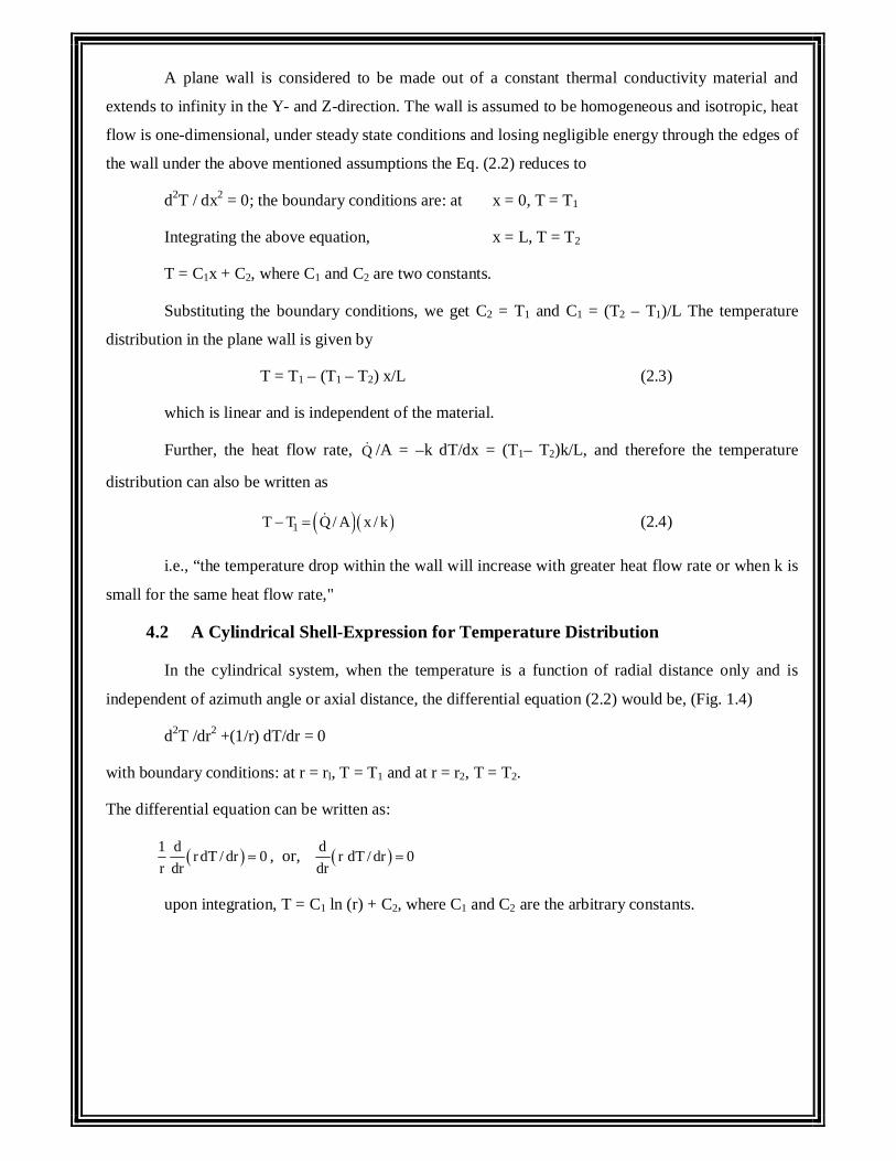
A plane wall is considered to be made out of a constant thermal conductivity material and
extends to infinity in the Y- and Z-direction. The wall is assumed to be homogeneous and isotropic, heat
flow is one-dimensional, under steady state conditions and losing negligible energy through the edges of
the wall under the above mentioned assumptions the Eq. (2.2) reduces to
d2T / dx2 = 0; the boundary conditions are: at x = 0, T = T1
Integrating the above equation, x = L, T = T2
T = C1x + C2, where C1 and C2 are two constants.
Substituting the boundary conditions, we get C2 = T1 and C1 = (T2 – T1)/L The temperature
distribution in the plane wall is given by
T = T1 – (T1 – T2) x/L (2.3)
which is linear and is independent of the material.
Further, the heat flow rate, Q /A = –k dT/dx = (T1– T2)k/L, and therefore the temperature
distribution can also be written as
1T T Q/ A x / k (2.4)
i.e., “the temperature drop within the wall will increase with greater heat flow rate or when k is
small for the same heat flow rate,"
4.2 A Cylindrical Shell-Expression for Temperature Distribution
In the cylindrical system, when the temperature is a function of radial distance only and is
independent of azimuth angle or axial distance, the differential equation (2.2) would be, (Fig. 1.4)
d2T /dr2 +(1/r) dT/dr = 0
with boundary conditions: at r = rl, T = T1 and at r = r2, T = T2.
The differential equation can be written as:
1 d r dT / dr 0r dr
, or, d r dT / dr 0dr
upon integration, T = C1 ln (r) + C2, where C1 and C2 are the arbitrary constants.
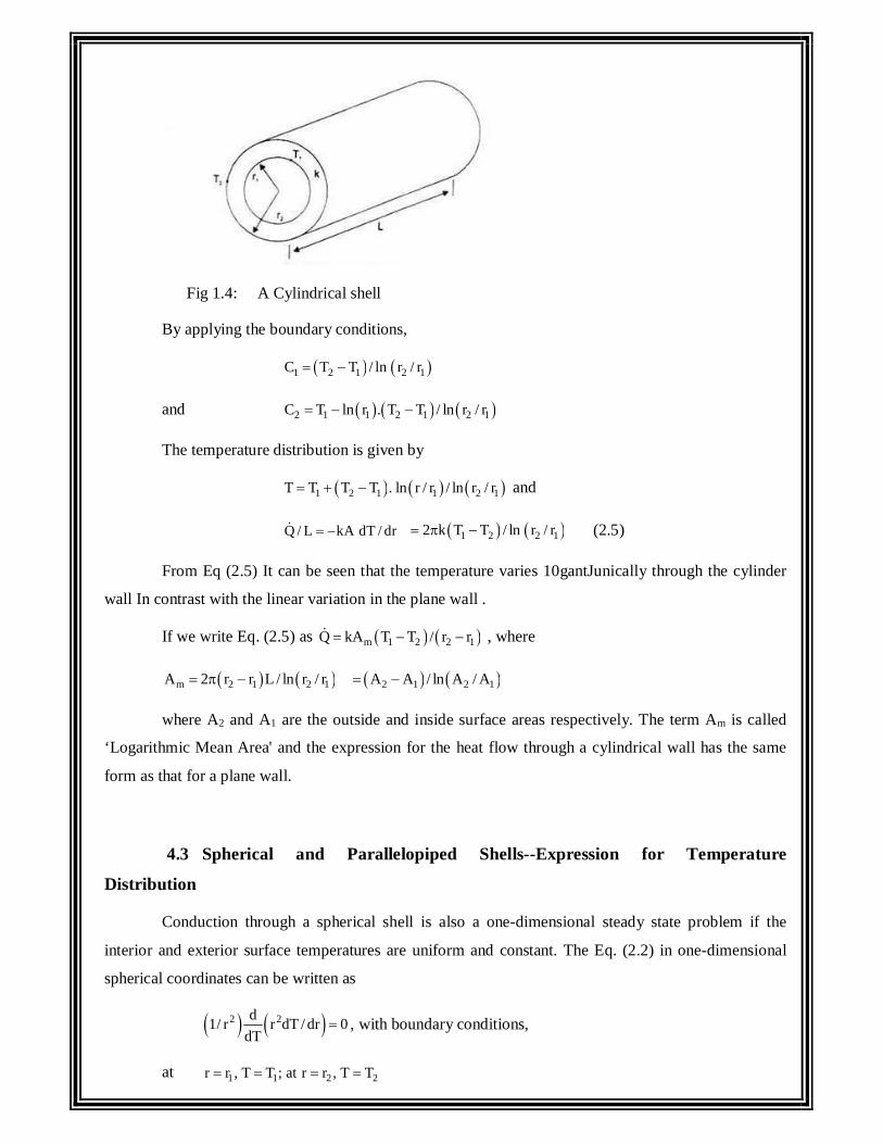
Fig 1.4: A Cylindrical shell
By applying the boundary conditions,
1 2 1 2 1C T T / ln r / r
and 2 1 1 2 1 2 1C T ln r . T T / ln r / r
The temperature distribution is given by
1 2 1 1 2 1T T T T . ln r / r / ln r / r and
Q / L kA dT / dr 1 2 2 12 k T T / ln r / r (2.5)
From Eq (2.5) It can be seen that the temperature varies 10gantJunically through the cylinder
wall In contrast with the linear variation in the plane wall .
If we write Eq. (2.5) as m 1 2 2 1Q kA T T / r r , where
m 2 1 2 1A 2 r r L / ln r / r 2 1 2 1A A / ln A / A
where A2 and A1 are the outside and inside surface areas respectively. The term Am is called
‘Logarithmic Mean Area' and the expression for the heat flow through a cylindrical wall has the same
form as that for a plane wall.
4.3 Spherical and Parallelopiped Shells--Expression for Temperature
Distribution
Conduction through a spherical shell is also a one-dimensional steady state problem if the
interior and exterior surface temperatures are uniform and constant. The Eq. (2.2) in one-dimensional
spherical coordinates can be written as
2 2d1/ r r dT / dr 0dT
, with boundary conditions,
at 1 1 2 2r r , T T ; at r r , T T
or, 2d r dT / dr 0dr
and upon integration, T = –C1/r + C2, where c1 and c2 are constants. substituting the boundary
conditions,
1 1 2 1 2 1 2C T T r r / r r , and 2 1 1 2 1 2 1 1 2C T T T r r / r r r
The temperature distribution m the spherical shell is given by
1 2 1 2 11
2 1 1
T T r r r rT T
r r r r
(2.6)
and the temperature distribution associated with radial conduction through a sphere is
represented by a hyperbola. The rate of heat conduction is given by
½1 2 1 2 2 1 1 2 1 2 2 1Q 4 k T T r r / r r k A A T T / r r (2.7)
where 21 1A 4 and 2
2 2A 4 r
If Al is approximately equal to A2 i.e., when the shell is very thin,
1 2 2 1Q kA T T / r r ; and 1 2Q / A T T / r / k
which is an expression for a flat slab.
The above equation (2.7) can also be used as an approximation for parallelopiped shells which
have a smaller inner cavity surrounded by a thick wall, such as a small furnace surrounded by a large
thickness of insulating material, although the h eat flow especially in the corners, cannot be strictly
considered one-dimensional. It has been suggested that for (A2/A1) > 2, the rate of heat flow can be
approximated by the above equation by multiplying the geometric mean area
Am = (A1 A2)½ by a correction factor 0.725.]
4.4 Composite Surfaces
There are many practical situations where different materials are placed m layers to form
composite surfaces, such as the wall of a building, cylindrical pipes or spherical shells having different
layers of insulation. Composite surfaces may involve any number of series and parallel thermal circuits.
4.5 Heat Transfer Rate through a Composite Wall
Let us consider a general case of a composite wall as shown m Fig. 1.5 There are ‘n’ layers of
different materials of thicknesses L1, L2, etc and having thermal conductivities kl, k2, etc. On one side of
the composite wall, there is a fluid A at temperature TA and on the other side of the wall there is a fluid
B at temperature TB. The convective heat transfer coefficients on the two sides of the wall are hA and hB
respectively. The system is analogous to a series of resistances as shown in the figure.

Fig 1.5 Heat transfer through a composite wall
4.6 The Equivalent Thermal Conductivity The process of heat transfer through compos lie and plane walls can be more conveniently
compared by introducing the concept of 'equivalent thermal conductivity', keq. It is defined as:
n n
eq i i ii 1 i 1
k L L / k
(2.8)
Total thickeness of the composite wall=Total thermal resistance of the composite wall
And, its value depends on the thermal and physical properties and the thickness of each
constituent of the composite structure.
Example 1.2 A furnace wall consists of 150 mm thick refractory brick (k = 1.6 W/mK) and 150 mm
thick insulating fire brick (k = 0.3 W/mK) separated by an au gap (resistance 0 16 K/W).
The outside walls covered with a 10 mm thick plaster (k = 0.14 W/mK). The
temperature of hot gases is 1250°C and the room temperature is 25°C. The convective
heat transfer coefficient for gas side and air side is 45 W/m2K and 20 W/m2K. Calculate
(i) the rate of heat flow per unit area of the wall surface (ii) the temperature at the
outside and Inside surface of the wall and (iii) the rate of heat flow when the air gap is
not there.
Solution: Using the nomenclature of Fig. 2.3, we have per m2 of the area, hA = 45, and RA =
1/hA = 1/45 = 0.0222; hB = 20, and RB = 1120 = 0.05
Resistance of the refractory brick, R1 = L1/k1 = 0.15/1.6 = 0.0937
Resistance of the insulating brick, R3 = L3/k3 = 0.15/0.30 = 0.50
The resistance of the air gap, R2 = 0.16
Resistance of the plaster, R4 = 0.01/0.14 = 0.0714
Total resistance = 0.8973, m2K/W
Heat flow rate = T/R = (1250-25)/0.8973= 13662 W/m2
Temperature at the inner surface of the wall
= TA – 1366.2 × 0.0222 = 1222.25
Temperature at the outer surface of the wall
= TB + 1366.2 × 0.05 = 93.31 °C
When the air gap is not there, the total resistance would be
0.8973 - 0.16 = 0.7373
and the heat flow rate = (1250 – 25)/0/7373 = 1661.46 W/m2
The temperature at the inner surface of the wall
= 1250 – 1660.46 × 0.0222 = 1213.12°C
i.e., when the au gap is not there, the heat flow rate increases but the temperature at the inner
surface of the wall decreases.
The overall heat transfer coefficient U with and without the air gap is
U= Q/A / T
= 13662 / (1250 – 25) = 1.115 Wm2 °C
and 1661.46/l225 = 1356 W/m2oC
The equivalent thermal conductivity of the system without the air gap
keq = (0.15 + 0.15 + 0.01)/(0.0937 + 0.50 + 0.0714) = 0.466 W/mK.
Example 1.2 A brick wall (10 cm thick, k = 0.7 W/m°C) has plaster on one side of the wall (thickness 4
cm, k = 0.48 W/m°C). What thickness of an insulating material (k = 0.065 W moC) should
be added on the other side of the wall such that the heat loss through the wall IS reduced
by 80 percent.
Solution: When the insulating material is not there, the resistances are:
R1 = L1/k1 = 0.1/0.7 = 0.143
and R2 = 0.04/0.48 = 0.0833
Total resistance = 0.2263
Let the thickness of the insulating material is L3. The resistance would then be
L3/0.065 = 15.385 L3
Since the heat loss is reduced by 80% after the insulation is added.
Q with insulation R without insulation0.2Q without insulation R with insulation
or, the resistance with insulation = 0.2263/0.2 = 01.1315
and, 15385 L3 = I 1315 – 0.2263 = 0.9052
L3 = 0.0588 m = 58.8 mm
Example 1.3 An ice chest IS constructed of styrofoam (k = 0.033 W/mK) having inside dimensions
25 by 40 by 100 cm. The wall thickness is 4 cm. The outside surface of the chest is
exposed to air at 25°C with h = 10 W/m2K. If the chest is completely filled with ice,
calculate the time for ice to melt completely. The heat of fusion for water is 330 kJ/kg.
Solution: If the heat loss through the comers and edges are Ignored, we have three walls of walls
through which conduction heat transfer Will occur.
(a) 2 walls each having dimensions 25 cm × 40 cm × 4 cm
(b) 2 walls each having dimensions 25 cm × 100 cm × 4 cm
(c) 2 walls each having dimensions 40 cm × 100 cm × 4 cm
The surface area for convection heat transfer (based on outside dimensions)
2(33 × 48 + 33 × 108 + 48 × 108) × 10–4 = 2.0664 m2.
Resistance due to conduction and convection can be written as
0.04 0.04 0.04 120.033 0.25 0.4 0.033 0.25 1 0.033 0.4 1 10 2.0664
= 40 + 0.0484 = 40.0484 K/W
Q T / R = (25 – 0.0) / 40.0484 = 0.624 W
Inside volume of the container - 0.25 × 04 × 1 = 0.1 m3
Mass of Ice stored = 800 × 0.1 = 80 kg; taking the density of Ice as 800 kg/m3. The time
required to melt 80 kg of ice is
80 330 1000t 490 days0.624 3600 24
Example1.4 A composite furnace wall is to be constructed with two layers of materials (k1 = 2.5
W/moC and k2 = 0.25 W/moC). The convective heat transfer coefficient at the inside and
outside surfaces are expected to be 250 W/m2oC and 50 W/m2oC respectively. The
temperature of gases and air are 1000 K and 300 K. If the interface temperature is 650 K,
Calculate (i) the thickness of the two materials when the total thickness does not exceed 65
cm and (ii) the rate of heat flow. Neglect radiation.
Solution: Let the thickness of one material (k = 2.5 W / mK) is xm, then the thickness of the other
material (k = 0.25 W/mK) will be (0.65 –x)m.
For steady state condition, we can write
Q 1000 650 1000 300
1 x 0.65 xA 1 x 1250 2.5 250 2.5 0.25 50
700 0.004 0.4x 350 0.004 0.4x 4 0.65 x 0.02
(i) 6x = 3.29 and x= 0.548 m.
and the thickness of the other material = 0.102 m.
(ii) Q / A = (350) / (0.004 + 0.4 × 0.548) = 1.568 kW/m2
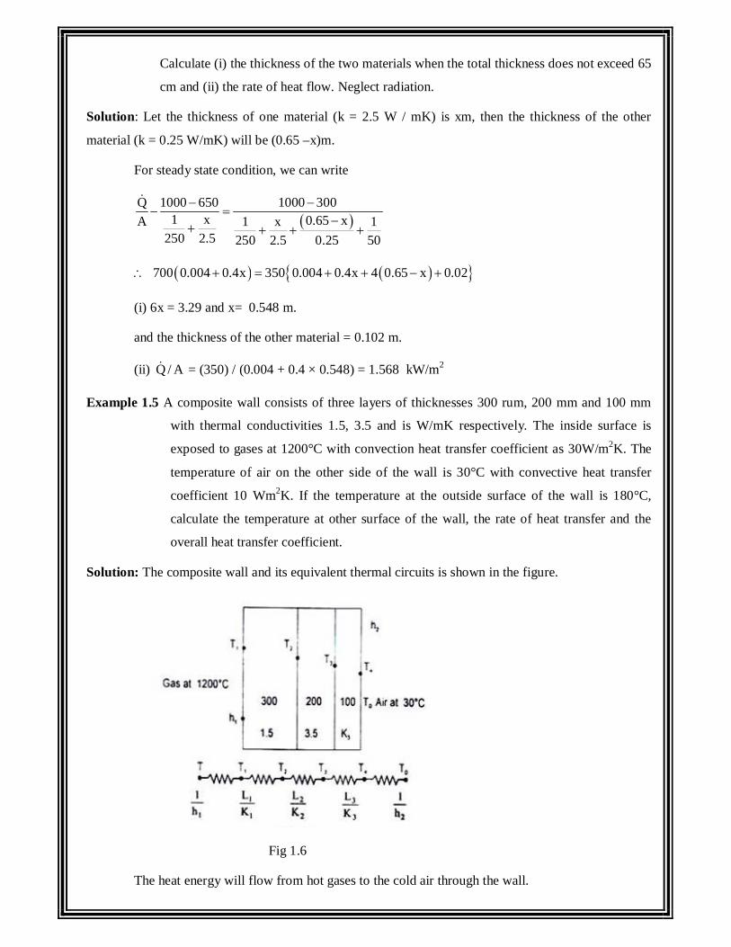
Example 1.5 A composite wall consists of three layers of thicknesses 300 rum, 200 mm and 100 mm
with thermal conductivities 1.5, 3.5 and is W/mK respectively. The inside surface is
exposed to gases at 1200°C with convection heat transfer coefficient as 30W/m2K. The
temperature of air on the other side of the wall is 30°C with convective heat transfer
coefficient 10 Wm2K. If the temperature at the outside surface of the wall is 180°C,
calculate the temperature at other surface of the wall, the rate of heat transfer and the
overall heat transfer coefficient.
Solution: The composite wall and its equivalent thermal circuits is shown in the figure.
Fig 1.6
The heat energy will flow from hot gases to the cold air through the wall.
From the electric Circuit, we have
22 4 0Q / A h T T 10 180 30 1500 W / m
also, 1 1Q / A h 1200 T
o1T 1200 1500 / 30 1150 C
1 2 1 1Q / A T T / L / k
2 1T T 1500 0.3/1.5 850
Similarly, 2 3 2 2Q / A T T / L / k
o3 2T T 1500 0.2 / 3.5 764.3 C
and 3 4 3 3Q / A T T / L / k
3 3L / k 764.3 180 /1500 and k3 = 0.256 W/mK
Check:
Q / A 1200 30 / R;
where 1 1 1 2 2 3 3 2R 1/ h L / k L / k L / k 1/ h
R 1/ 30 0.3/1.5 0.2 / 3.5 0.1/ 0.256 1/10 0.75
and 2Q / A 1170 / 0.78 1500 W / m
The overall heat transfer coefficient, 2U 1/ R 1/ 0.78 1.282 W / m K
Since the gas temperature is very high, we should consider the effects of radiation also.
Assuming the heat transfer coefficient due to radiation = 3.0 W/m2K the electric circuit would be:
The combined resistance due to convection and radiation would be
2oc r
1 2
c r
1 1 1 1 1 h h 60W / m C1 1R R Rh h
1 1Q / A 1500 60 T T 60 1200 T
o1
1500T 1200 1175 C60
again, o1 2 1 1 2 1Q / A T T / L / k T T 1500 0.3/1.5 875 C
and o3 2T T 1500 0.2 / 3.5 789.3 C
3 3 3L / k 789.3 180 /1500; k 0.246 W / mK
1 0.3 0.2 0.2 0.1 1R 0.7860 1.5 1.5 3.5 0.246 10
and 2U 1/ R 1.282 W / m K
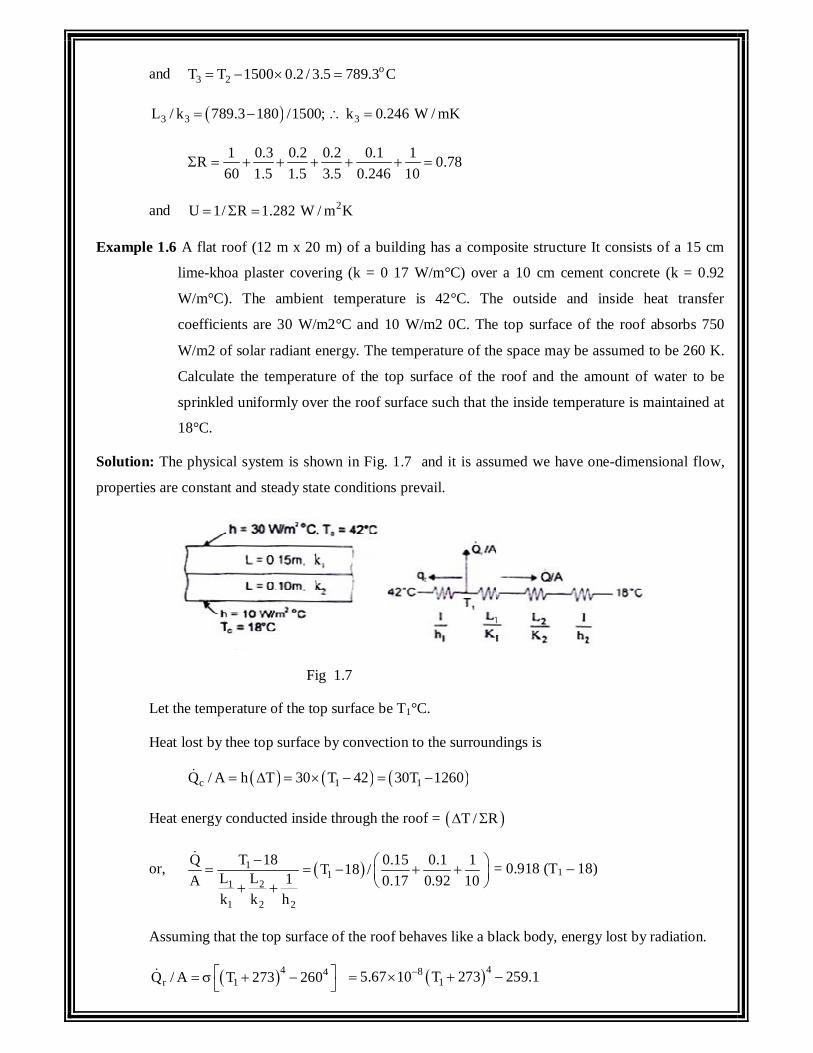
Example 1.6 A flat roof (12 m x 20 m) of a building has a composite structure It consists of a 15 cm
lime-khoa plaster covering (k = 0 17 W/m°C) over a 10 cm cement concrete (k = 0.92
W/m°C). The ambient temperature is 42°C. The outside and inside heat transfer
coefficients are 30 W/m2°C and 10 W/m2 0C. The top surface of the roof absorbs 750
W/m2 of solar radiant energy. The temperature of the space may be assumed to be 260 K.
Calculate the temperature of the top surface of the roof and the amount of water to be
sprinkled uniformly over the roof surface such that the inside temperature is maintained at
18°C.
Solution: The physical system is shown in Fig. 1.7 and it is assumed we have one-dimensional flow,
properties are constant and steady state conditions prevail.
Fig 1.7
Let the temperature of the top surface be T1°C.
Heat lost by thee top surface by convection to the surroundings is
c 1 1Q / A h T 30 T 42 30T 1260
Heat energy conducted inside through the roof = T / R
or, 11
1 2
1 2 2
T 18Q 0.15 0.1 1T 18 /L L 1A 0.17 0.92 10k k h
= 0.918 (T1 – 18)
Assuming that the top surface of the roof behaves like a black body, energy lost by radiation.
4 4r 1Q / A T 273 260 48
15.67 10 T 273 259.1
By making an energy balance on the top surface of the roof,
Energy coming in = Energy going out
750 = (30T, -1260)+ 0.918 (T1-18) + 5.67 × 10⁻⁸ (T1 + 273)4 - 259.1
or, 2285.624 = 30.918 T1 + 5.67 × 10⁻⁸ (T1 + 273)4
Solving by trial and error, T1 = 53.4°C, and the total energy conducted through the roof per
hour is
0.918 (53.4 – 18) × (12 × 20) × 3600 = 28077.58 kJ/hr
Assuming the latent heat of vaporization of water as 2430 kJ/kg, the quantity of water to be
sprinkled over the surface such that it evaporates and consumes 28077.58 kJ/hr, is
wM = 28077.58/2430 = 11.55 kg/hr.
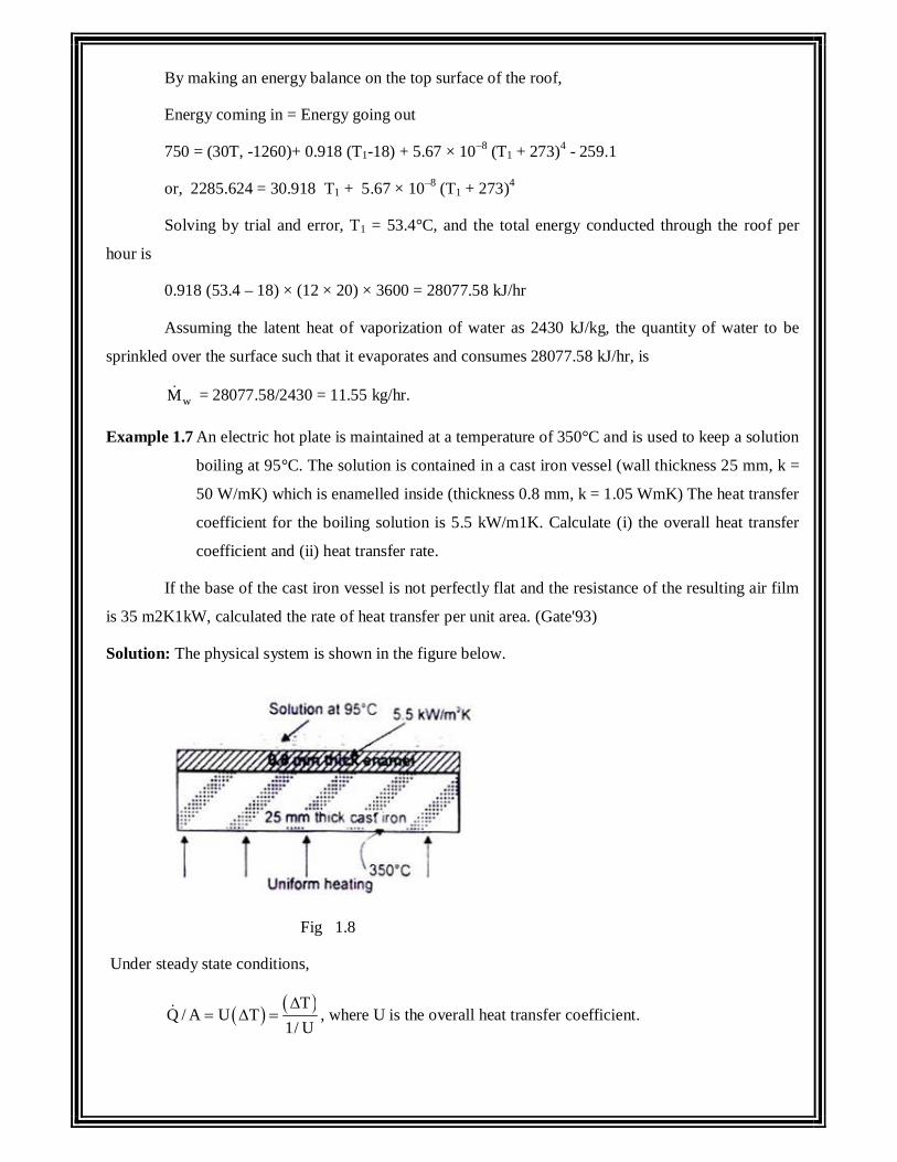
Example 1.7 An electric hot plate is maintained at a temperature of 350°C and is used to keep a solution
boiling at 95°C. The solution is contained in a cast iron vessel (wall thickness 25 mm, k =
50 W/mK) which is enamelled inside (thickness 0.8 mm, k = 1.05 WmK) The heat transfer
coefficient for the boiling solution is 5.5 kW/m1K. Calculate (i) the overall heat transfer
coefficient and (ii) heat transfer rate.
If the base of the cast iron vessel is not perfectly flat and the resistance of the resulting air film
is 35 m2K1kW, calculated the rate of heat transfer per unit area. (Gate'93)
Solution: The physical system is shown in the figure below.
Fig 1.8
Under steady state conditions,
TQ / A U T
1/ U
, where U is the overall heat transfer coefficient.
1 2
1 2
T TL L 1Rk k h
Therefore,
1 2
1 2
L L 11/ Uk k h
0.025 0.0008 1 0.0014450 1.05 5500
U = 692.65 W/m2K
Q / A U T = 692.65 × (350 – 95) = 176.65 kW/m2.
With the presence of air film at the base, the total resistance to heat flow would be:
0.00144 + 0.035 = 0.03644 m2K/W
and the rate of heat transfer, Q / A = 255/0.03644 = 7 kW/m2.
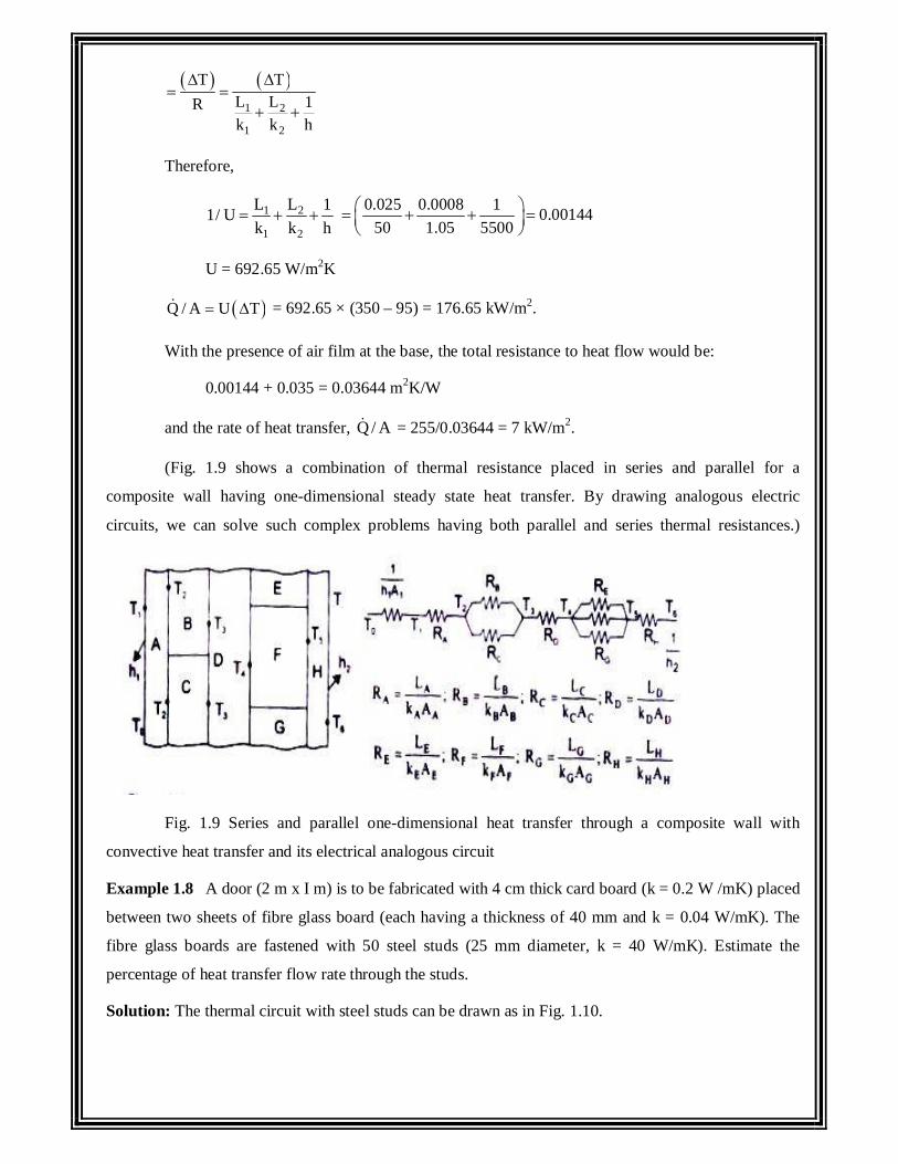
(Fig. 1.9 shows a combination of thermal resistance placed in series and parallel for a
composite wall having one-dimensional steady state heat transfer. By drawing analogous electric
circuits, we can solve such complex problems having both parallel and series thermal resistances.)
Fig. 1.9 Series and parallel one-dimensional heat transfer through a composite wall with
convective heat transfer and its electrical analogous circuit
Example 1.8 A door (2 m x I m) is to be fabricated with 4 cm thick card board (k = 0.2 W /mK) placed
between two sheets of fibre glass board (each having a thickness of 40 mm and k = 0.04 W/mK). The
fibre glass boards are fastened with 50 steel studs (25 mm diameter, k = 40 W/mK). Estimate the
percentage of heat transfer flow rate through the studs.
Solution: The thermal circuit with steel studs can be drawn as in Fig. 1.10.
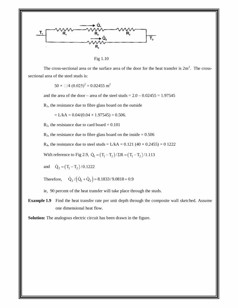
Fig 1.10
The cross-sectional area or the surface area of the door for the heat transfer is 2m2. The cross-
sectional area of the steel studs is:
50 × /4 (0.025)2 = 0.02455 m2
and the area of the door – area of the steel studs = 2.0 – 0.02455 = 1.97545
R1, the resistance due to fibre glass board on the outside
= L/kA = 0.04/(0.04 × 1.97545) = 0.506.
R2, the resistance due to card board = 0.101
R3, the resistance due to fibre glass board on the inside = 0.506
R4, the resistance due to steel studs = L/kA = 0.121 (40 × 0.2455) = 0 1222
With reference to Fig 2.9, 1 1 2 1 2Q T T / R T T /1.113
and 2 1 2Q T T / 0.1222
Therefore, 2 1 2Q / Q Q 8.1833/ 9.0818 0.9
ie, 90 percent of the heat transfer will take place through the studs.
Example 1.9 Find the heat transfer rate per unit depth through the composite wall sketched. Assume
one dimensional heat flow.
Solution: The analogous electric circuit has been drawn in the figure.
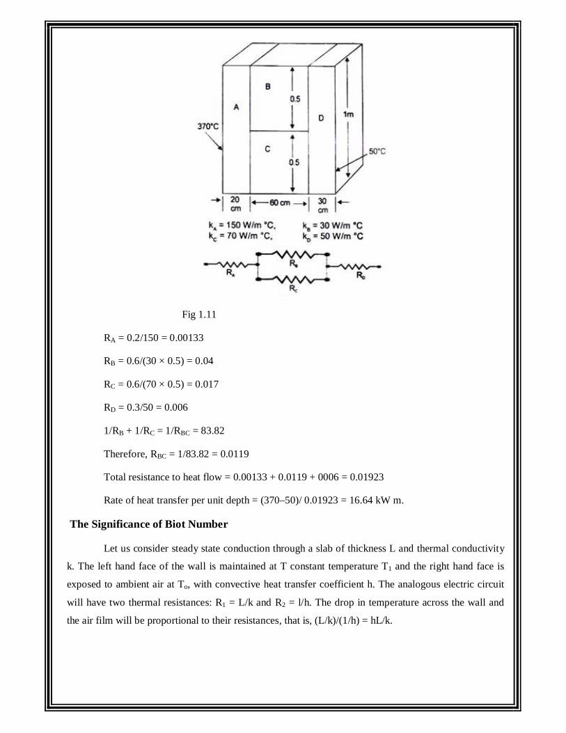
Fig 1.11
RA = 0.2/150 = 0.00133
RB = 0.6/(30 × 0.5) = 0.04
RC = 0.6/(70 × 0.5) = 0.017
RD = 0.3/50 = 0.006
1/RB + 1/RC = 1/RBC = 83.82
Therefore, RBC = 1/83.82 = 0.0119
Total resistance to heat flow = 0.00133 + 0.0119 + 0006 = 0.01923
Rate of heat transfer per unit depth = (370–50)/ 0.01923 = 16.64 kW m.
The Significance of Biot Number
Let us consider steady state conduction through a slab of thickness L and thermal conductivity
k. The left hand face of the wall is maintained at T constant temperature T1 and the right hand face is
exposed to ambient air at To, with convective heat transfer coefficient h. The analogous electric circuit
will have two thermal resistances: R1 = L/k and R2 = l/h. The drop in temperature across the wall and
the air film will be proportional to their resistances, that is, (L/k)/(1/h) = hL/k.
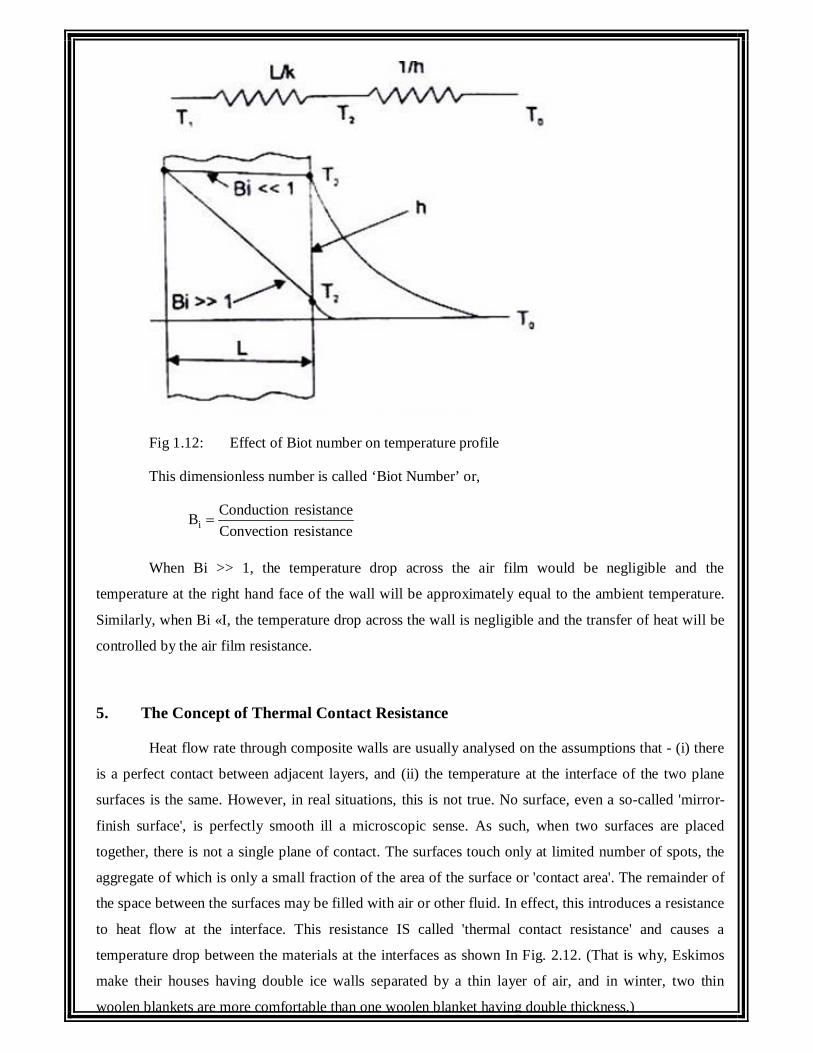
Fig 1.12: Effect of Biot number on temperature profile
This dimensionless number is called ‘Biot Number’ or,
iConduction resistanceBConvection resistance
When Bi >> 1, the temperature drop across the air film would be negligible and the
temperature at the right hand face of the wall will be approximately equal to the ambient temperature.
Similarly, when Bi «I, the temperature drop across the wall is negligible and the transfer of heat will be
controlled by the air film resistance.
5. The Concept of Thermal Contact Resistance
Heat flow rate through composite walls are usually analysed on the assumptions that - (i) there
is a perfect contact between adjacent layers, and (ii) the temperature at the interface of the two plane
surfaces is the same. However, in real situations, this is not true. No surface, even a so-called 'mirror-
finish surface', is perfectly smooth ill a microscopic sense. As such, when two surfaces are placed
together, there is not a single plane of contact. The surfaces touch only at limited number of spots, the
aggregate of which is only a small fraction of the area of the surface or 'contact area'. The remainder of
the space between the surfaces may be filled with air or other fluid. In effect, this introduces a resistance
to heat flow at the interface. This resistance IS called 'thermal contact resistance' and causes a
temperature drop between the materials at the interfaces as shown In Fig. 2.12. (That is why, Eskimos
make their houses having double ice walls separated by a thin layer of air, and in winter, two thin
woolen blankets are more comfortable than one woolen blanket having double thickness.)
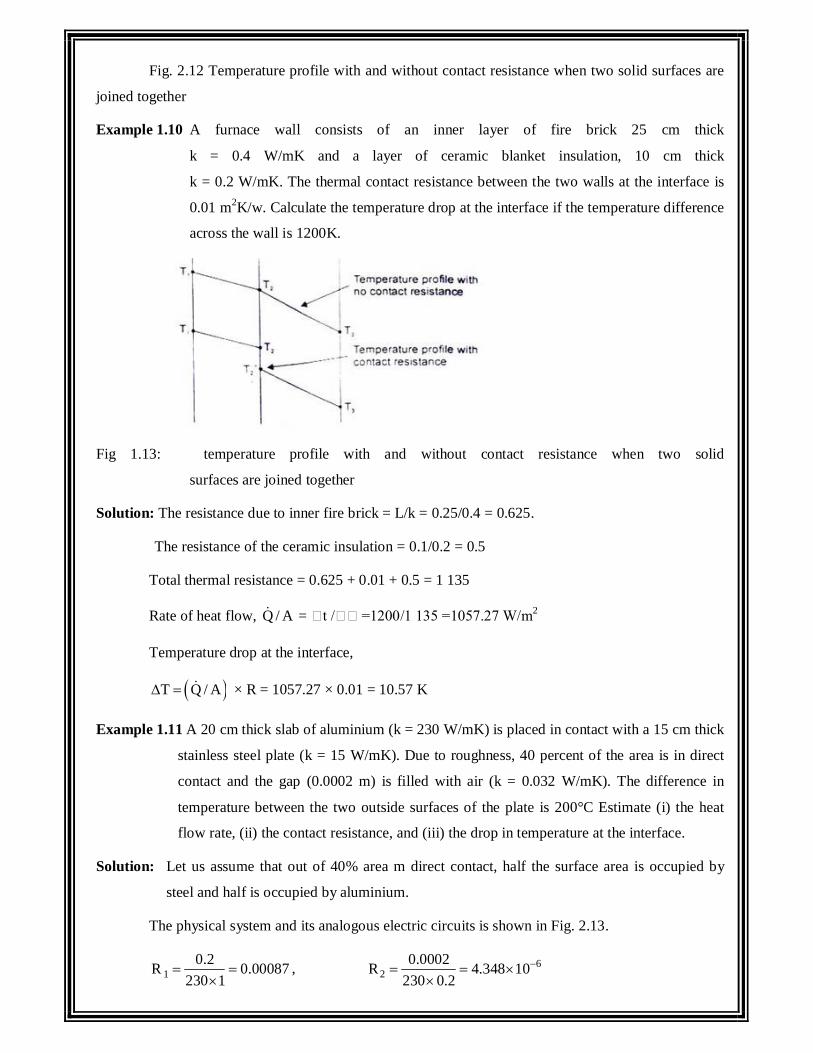
Fig. 2.12 Temperature profile with and without contact resistance when two solid surfaces are
joined together
Example 1.10 A furnace wall consists of an inner layer of fire brick 25 cm thick
k = 0.4 W/mK and a layer of ceramic blanket insulation, 10 cm thick
k = 0.2 W/mK. The thermal contact resistance between the two walls at the interface is
0.01 m2K/w. Calculate the temperature drop at the interface if the temperature difference
across the wall is 1200K.
Fig 1.13: temperature profile with and without contact resistance when two solid
surfaces are joined together
Solution: The resistance due to inner fire brick = L/k = 0.25/0.4 = 0.625.
The resistance of the ceramic insulation = 0.1/0.2 = 0.5
Total thermal resistance = 0.625 + 0.01 + 0.5 = 1 135
Rate of heat flow, Q / A = t / =1200/1 135 =1057.27 W/m2
Temperature drop at the interface,
T Q / A × R = 1057.27 × 0.01 = 10.57 K
Example 1.11 A 20 cm thick slab of aluminium (k = 230 W/mK) is placed in contact with a 15 cm thick
stainless steel plate (k = 15 W/mK). Due to roughness, 40 percent of the area is in direct
contact and the gap (0.0002 m) is filled with air (k = 0.032 W/mK). The difference in
temperature between the two outside surfaces of the plate is 200°C Estimate (i) the heat
flow rate, (ii) the contact resistance, and (iii) the drop in temperature at the interface.
Solution: Let us assume that out of 40% area m direct contact, half the surface area is occupied by
steel and half is occupied by aluminium.
The physical system and its analogous electric circuits is shown in Fig. 2.13.
10.2R 0.00087
230 1
, 6
20.0002R 4.348 10
230 0.2
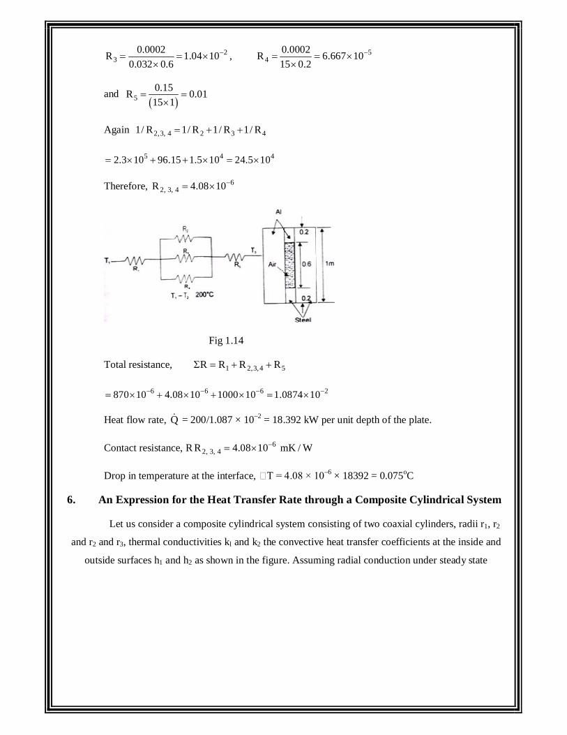
23
0.0002R 1.04 100.032 0.6
, 54
0.0002R 6.667 1015 0.2
and 5
0.15R 0.0115 1
Again 2,3, 4 2 3 41/ R 1/ R 1/ R 1/ R
5 4 42.3 10 96.15 1.5 10 24.5 10
Therefore, 62, 3, 4R 4.08 10
Fig 1.14
Total resistance, 1 2,3,4 5R R R R
6 6 6 2870 10 4.08 10 1000 10 1.0874 10
Heat flow rate, Q = 200/1.087 × 10–2 = 18.392 kW per unit depth of the plate.
Contact resistance, R 62, 3, 4R 4.08 10 mK / W
Drop in temperature at the interface, T = 4.08 × 10–6 × 18392 = 0.075oC
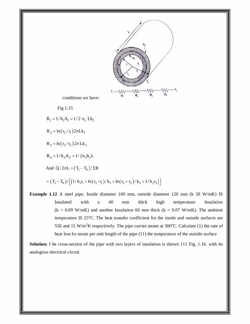
6. An Expression for the Heat Transfer Rate through a Composite Cylindrical System
Let us consider a composite cylindrical system consisting of two coaxial cylinders, radii r1, r2
and r2 and r3, thermal conductivities kl and k2 the convective heat transfer coefficients at the inside and
outside surfaces h1 and h2 as shown in the figure. Assuming radial conduction under steady state
conditions we have:
Fig 1.15
1 1 1 1 1R 1/ h A 1/ 2 Lh
2 2 1 1R ln r / r 2 Lk
3 3 2 2R ln r / r 2 Lk
4 2 2 3 2R 1/ h A 1/ 2 h L
And 1 0Q / 2 L T T / R
1 0 1 1 2 1 1 3 2 2 2 3T T / 1/ h r ln r / r / k ln r r / k 1/ h r
Example 1.12 A steel pipe. Inside diameter 100 mm, outside diameter 120 mm (k 50 W/mK) IS
Insulated with a 40 mm thick high temperature Insulation
(k = 0.09 W/mK) and another Insulation 60 mm thick (k = 0.07 W/mK). The ambient
temperature IS 25°C. The heat transfer coefficient for the inside and outside surfaces are
550 and 15 W/m2K respectively. The pipe carries steam at 300oC. Calculate (1) the rate of
heat loss by steam per unit length of the pipe (11) the temperature of the outside surface
Solution: I he cross-section of the pipe with two layers of insulation is shown 111 Fig. 1.16. with its
analogous electrical circuit.
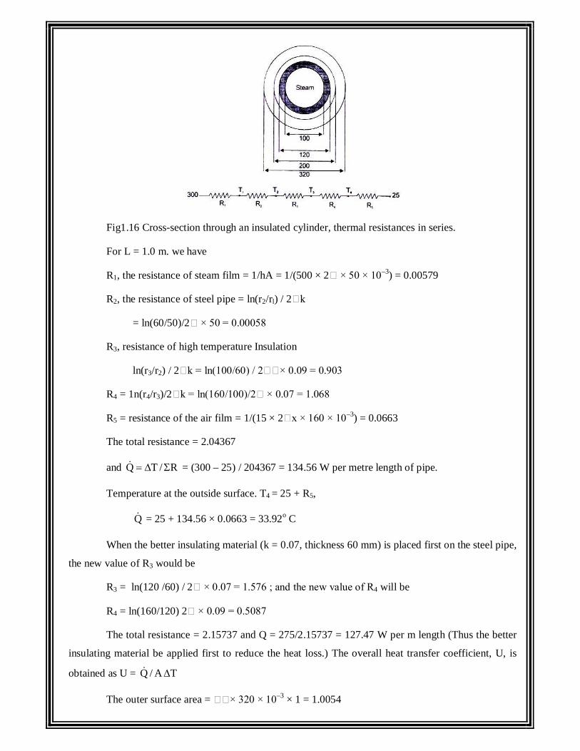
Fig1.16 Cross-section through an insulated cylinder, thermal resistances in series.
For L = 1.0 m. we have
R1, the resistance of steam film = 1/hA = 1/(500 × 2 × 50 × 10–3) = 0.00579
R2, the resistance of steel pipe = ln(r2/rl) / 2 k
= ln(60/50)/2 × 50 = 0.00058
R3, resistance of high temperature Insulation
ln(r3/r2) / 2 k = ln(100/60) / 2 × 0.09 = 0.903
R4 = 1n(r4/r3)/2 k = ln(160/100)/2 × 0.07 = 1.068
R5 = resistance of the air film = 1/(15 × 2 x × 160 × 10–3) = 0.0663
The total resistance = 2.04367
and Q T / R = (300 – 25) / 204367 = 134.56 W per metre length of pipe.
Temperature at the outside surface. T4 = 25 + R5,
Q = 25 + 134.56 × 0.0663 = 33.92o C
When the better insulating material (k = 0.07, thickness 60 mm) is placed first on the steel pipe,
the new value of R3 would be
R3 = ln(120 /60) / 2 × 0.07 = 1.576 ; and the new value of R4 will be
R4 = ln(160/120) 2 × 0.09 = 0.5087
The total resistance = 2.15737 and Q = 275/2.15737 = 127.47 W per m length (Thus the better
insulating material be applied first to reduce the heat loss.) The overall heat transfer coefficient, U, is
obtained as U = Q / A T
The outer surface area = × 320 × 10–3 × 1 = 1.0054
and U = 134.56/(275 × 1.0054) = 0.487 W/m2 K.
Example 1.13 A steam pipe 120 mm outside diameter and 10m long carries steam at a pressure of 30
bar and 099 dry. Calculate the thickness of a lagging material (k = 0.99 W/mK) provided
on the steam pipe such that the temperature at the outside surface of the insulated pipe
does not exceed 32°C when the steam flow rate is 1 kg/s and the dryness fraction of
steam at the exit is 0.975 and there is no pressure drop.
Solution: The latent heat of vaporization of steam at 30 bar = 1794 kJ/kg.
The loss of heat energy due to condensation of steam = 1794(0.99 – 0.975)
= 26.91 kJ/kg.
Since the steam flow rate is 1 kg/s, the loss of energy = 26.91 kW.
The saturation temperature of steam at 30 bar IS 233.84°C and assuming that the pipe material
offers negligible resistance to heat flow, the temperature at the outside surface of the uninsulated steam
pipe or at the inner surface of the lagging material is 233.84°C. Assuming one-dimensional radial heat
flow through the lagging material, we have
Q = (T1 – T2 )/[ln(r2/ rl)] 2 Lk
or, 26.91 × 1000 (W) = (233.84 – 32) × 2 × 10 × 0.99/1n(r/60)
ln (r/60) = 0.4666
r2/60 = exp (0.4666) = 1.5946
r2 = 95.68 mm and the thickness = 35.68 mm
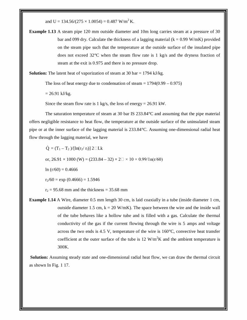
Example 1.14 A Wire, diameter 0.5 mm length 30 cm, is laid coaxially in a tube (inside diameter 1 cm,
outside diameter 1.5 cm, k = 20 W/mK). The space between the wire and the inside wall
of the tube behaves like a hollow tube and is filled with a gas. Calculate the thermal
conductivity of the gas if the current flowing through the wire is 5 amps and voltage
across the two ends is 4.5 V, temperature of the wire is 160°C, convective heat transfer
coefficient at the outer surface of the tube is 12 W/m2K and the ambient temperature is
300K.
Solution: Assuming steady state and one-dimensional radial heat flow, we can draw the thermal circuit
as shown In Fig. 1 17.
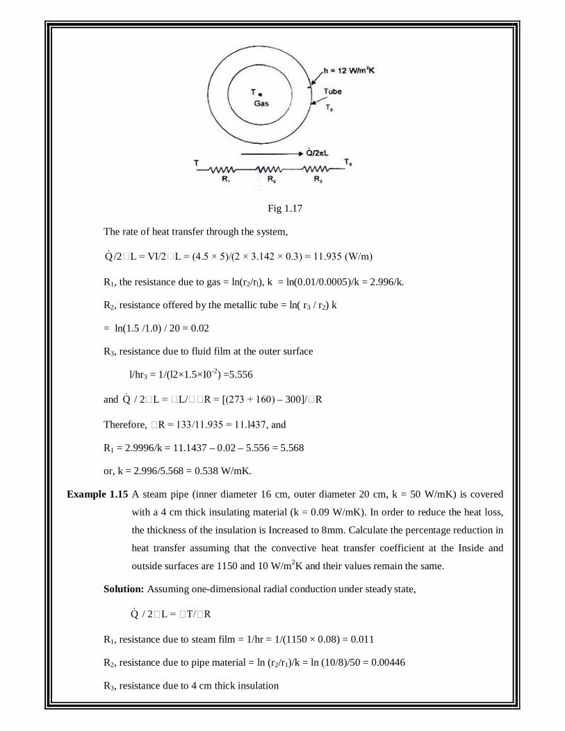
Fig 1.17
The rate of heat transfer through the system,
Q /2 L = VI/2 L = (4.5 × 5)/(2 × 3.142 × 0.3) = 11.935 (W/m)
R1, the resistance due to gas = ln(r2/rl), k = ln(0.01/0.0005)/k = 2.996/k.
R2, resistance offered by the metallic tube = ln( r3 / r2) k
= ln(1.5 /1.0) / 20 = 0.02
R3, resistance due to fluid film at the outer surface
l/hr3 = 1/(l2×1.5×I0-2) =5.556
and Q / 2 L = L/ R = [(273 + 160) – 300]/ R
Therefore, R = 133/11.935 = 11.l437, and
R1 = 2.9996/k = 11.1437 – 0.02 – 5.556 = 5.568
or, k = 2.996/5.568 = 0.538 W/mK.
Example 1.15 A steam pipe (inner diameter 16 cm, outer diameter 20 cm, k = 50 W/mK) is covered
with a 4 cm thick insulating material (k = 0.09 W/mK). In order to reduce the heat loss,
the thickness of the insulation is Increased to 8mm. Calculate the percentage reduction in
heat transfer assuming that the convective heat transfer coefficient at the Inside and
outside surfaces are 1150 and 10 W/m2K and their values remain the same.
Solution: Assuming one-dimensional radial conduction under steady state,
Q / 2 L = T/ R
R1, resistance due to steam film = 1/hr = 1/(1150 × 0.08) = 0.011
R2, resistance due to pipe material = ln (r2/r1)/k = ln (10/8)/50 = 0.00446
R3, resistance due to 4 cm thick insulation
= ln(r3/r2)/k = ln(14/10)/0.09 = 3.738
R4, resistance due to air film = 1/hr = 1/(10 × 0.14) = 0.714.
Therefore, Q / 2 L T / (0.011 + 0.00446 + 3.738 + 0.714) = 0.2386 T
When the thickness of the insulation is increased to 8 cm, the values of R3 and R4 will change.
R3 = ln(r3/r2)/k = ln(18/10)/0.09 = 6.53 ; and
R4 = 1/hr = 1/(10 × 0.18) = 0.556
Therefore, Q / 2 L T / (0.011 + 0.00446 + 6.53 + 0.556)
= T / 7.1 = 0.14084 T
Percentage reduction in heat transfer = 0.22386 0.14084
0.37 37%0.22386
Example 1.16 A small hemispherical oven is built of an inner layer of insulating fire brick 125 mm
thick (k = 0.31 W/mK) and an outer covering of 85% magnesia 40 mm thick (k = 0.05
W/mK). The inner surface of the oven is at 1073 K and the heat transfer coefficient for the
outer surface is 10 W/m2K, the room temperature is 20oC. Calculate the rate of heat loss
through the hemisphere if the inside radius is 0.6 m.
Solution: The resistance of the fire brick
= 2 1 1 20.725 0.6r r / 2 kr r 0.1478
2 0.31 0.6 0.725
The resistance of 85% magnesia
= 3 2 2 30.765 0.725r r / 2 kr r 0.2295
2 0.05 0.725 0.765
The resistance due to fluid film at the outer surface = 1/hA
1 0.229510 2 0.765 0.765
The resistance due to fluid film at the outer surface = 1/hA
1 0.027210 2 0.765 0.765
Rate of heat flow, 800 20Q T / R 1930W0.1478 0.2295 0.272
Example 1.17 A cylindrical tank with hemispherical ends is used to store liquid oxygen at – 180oC.
The diameter of the tank is 1.5 m and the total length is 8 m. The tank is covered with a
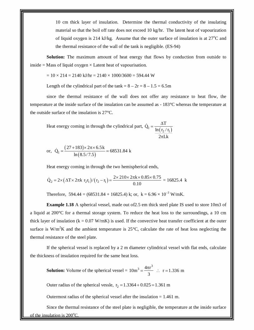
10 cm thick layer of insulation. Determine the thermal conductivity of the insulating
material so that the boil off rate does not exceed 10 kg/hr. The latent heat of vapourization
of liquid oxygen is 214 kJ/kg. Assume that the outer surface of insulation is at 27oC and
the thermal resistance of the wall of the tank is negligible. (ES-94)
Solution: The maximum amount of heat energy that flows by conduction from outside to
inside = Mass of liquid oxygen × Latent heat of vapourisation.
= 10 × 214 = 2140 kJ/hr = 2140 × 1000/3600 = 594.44 W
Length of the cylindrical part of the tank = 8 – 2r = 8 – 1.5 = 6.5m
since the thermal resistance of the wall does not offer any resistance to heat flow, the
temperature at the inside surface of the insulation can be assumed as - 183°C whereas the temperature at
the outside surface of the insulation is 27°C.
Heat energy coming in through the cylindrical part, 1
2 1
TQln r / r
2 Lk
or,
127 183 2 6.5k
Q 68531.84 kln 8.5 / 7.5
Heat energy coming in through the two hemispherical ends,
2 2 1 2 12 210 2 k 0.85 0.75Q 2 T 2 k r r / r r
0.10
= 16825.4 k
Therefore, 594.44 = (68531.84 + 16825.4) k; or, k = 6.96 × 10⁻³ W/mK.
Example 1.18 A spherical vessel, made out of2.5 em thick steel plate IS used to store 10m3 of
a liquid at 200°C for a thermal storage system. To reduce the heat loss to the surroundings, a 10 cm
thick layer of insulation (k = 0.07 W/rnK) is used. If the convective heat transfer coefficient at the outer
surface is W/m2K and the ambient temperature is 25°C, calculate the rate of heat loss neglecting the
thermal resistance of the steel plate.
If the spherical vessel is replaced by a 2 m diameter cylindrical vessel with flat ends, calculate
the thickness of insulation required for the same heat loss.
Solution: Volume of the spherical vessel = 3
3 4 r10m3
r 1.336 m
Outer radius of the spherical vessle, 2r 1.3364 0.025 1.361 m
Outermost radius of the spherical vessel after the insulation = 1.461 m.
Since the thermal resistance of the steel plate is negligible, the temperature at the inside surface
of the insulation is 200oC.
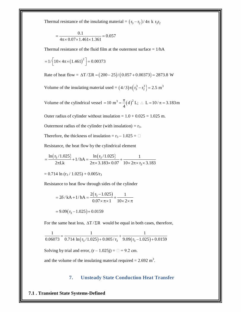
Thermal resistance of the insulating material = 3 2 3 2r r / 4 k r r
0.1 0.0574 0.07 1.461 1.361
Thermal resistance of the fluid film at the outermost surface = 1/hA
21/ 10 4 1.461 0.00373
Rate of heat flow = T / R 200 25 / 0.057 0.00373 2873.8 W
Volume of the insulating material used = 3 3 33 24 / 3 r r 2.5 m
Volume of the cylindrical vessel 2310 m d L; L 10 / 3.183m4
Outer radius of cylinder without insulation = 1.0 + 0.025 = 1.025 m.
Outermost radius of the cylinder (with insulation) = r3.
Therefore, the thickness of insulation = r3 – 1.025 =
Resistance, the heat flow by the cylindrical element
3 3
3
ln r /1.025 ln r /1.025 11/ hA2 Lk 2 3.183 0.07 10 2 r 3.183
= 0.714 ln (r3 / 1.025) + 0.005/r3
Resistance to heat flow through sides of the cylinder
32 r 1.025 12 / kA 1/ hA0.07 1 10 2
39.09 r 1.025 0.0159
For the same heat loss, T / R would be equal in both cases, therefore,
3 3 3
1 1 10.06073 0.714 ln r /1.025 0.005 / r 9.09 r 1.025 0.0159
Solving by trial and error, (r – 1.025j) = = 9.2 cm.
and the volume of the insulating material required = 2.692 m3.
7. Unsteady State Conduction Heat Transfer
7.1 . Transient State Systems-Defined
The process of heat transfer by conduction where the temperature varies with time and with
space coordinates, is called 'unsteady or transient'. All transient state systems may be broadly classified
into two categories:
(a) Non-periodic Heat Flow System - the temperature at any point within the system changes as
a non-linear function of time.
(b) Periodic Heat Flow System - the temperature within the system undergoes periodic changes
which may be regular or irregular but definitely cyclic.
There are numerous problems where changes in conditions result in transient temperature
distributions and they are quite significant. Such conditions are encountered in - manufacture of
ceramics, bricks, glass and heat flow to boiler tubes, metal forming, heat treatment, etc.
7.2. Biot and Fourier Modulus-Definition and Significance
Let us consider an initially heated long cylinder (L >> R) placed in a moving stream of fluid at
sT T , as shown In Fig. 3.1(a). The convective heat transfer coefficient at the surface is h, where,
Q = hA ( sT T )
This energy must be conducted to the surface, and therefore,
Q = -kA(dT / dr) r = R
or, h( sT T ) = -k(dT/dr)r=R -k(Tc-Ts)/R
where Tc is the temperature at the axis of the cylinder
By rearranging,(Ts - Tc) / ( sT T ) h/Rk (3.1)
The term, hR/k, IS called the 'BlOT MODULUS'. It is a dimensionless number and is the ratio
of internal heat flow resistance to external heat flow resistance and plays a fundamental role in transient
conduction problems involving surface convection effects. I t provides a measure 0 f the temperature
drop in the solid relative to the temperature difference between the surface and the fluid.
For Bi << 1, it is reasonable to assume a uniform temperature distribution across a solid at any
time during a transient process.
Founer Modulus - It is also a dimensionless number and is defind as
Fo= t/L2 (3.2)
where L is the characteristic length of the body, a is the thermal diffusivity, and t is the time
The Fourier modulus measures the magnitude of the rate of conduction relative to the change in
temperature, i.e., the unsteady effect. If Fo << 1, the change in temperature will be experienced by a
region very close to the surface.
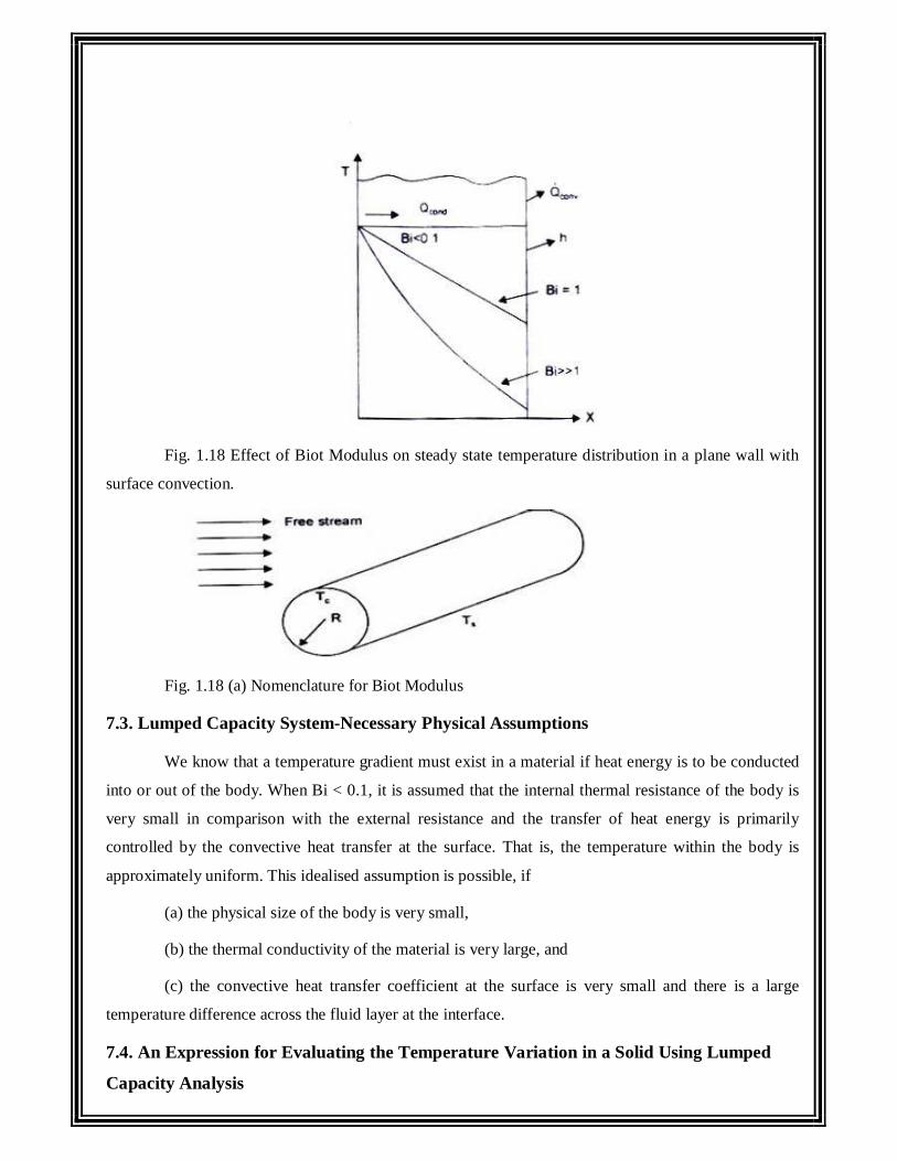
Fig. 1.18 Effect of Biot Modulus on steady state temperature distribution in a plane wall with
surface convection.
Fig. 1.18 (a) Nomenclature for Biot Modulus
7.3. Lumped Capacity System-Necessary Physical Assumptions
We know that a temperature gradient must exist in a material if heat energy is to be conducted
into or out of the body. When Bi < 0.1, it is assumed that the internal thermal resistance of the body is
very small in comparison with the external resistance and the transfer of heat energy is primarily
controlled by the convective heat transfer at the surface. That is, the temperature within the body is
approximately uniform. This idealised assumption is possible, if
(a) the physical size of the body is very small,
(b) the thermal conductivity of the material is very large, and
(c) the convective heat transfer coefficient at the surface is very small and there is a large
temperature difference across the fluid layer at the interface.
7.4. An Expression for Evaluating the Temperature Variation in a Solid Using Lumped
Capacity Analysis
Let us consider a small metallic object which has been suddenly immersed in a fluid during a
heat treatment operation. By applying the first law of
Heat flowing out of the body = Decrease in the internal thermal energy of
during a time dt the body during that time dt
or, hAs( T T )dt = - pCVdT
where As is the surface area of the body, V is the volume of the body and C is the specific heat
capacity.
or, (hA/ CV)dt = - dT /(T T )
with the initial condition being: at t = 0, T = Ts
The solution is : ( T T )/( sT T ) = exp(-hA / CV)t (3.3)
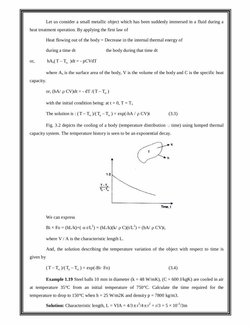
Fig. 3.2 depicts the cooling of a body (temperature distribution time) using lumped thermal
capacity system. The temperature history is seen to be an exponential decay.
We can express
Bi × Fo = (hL/k)×( t/L2) = (hL/k)(k/ C)(t/L2) = (hA/ CV)t,
where V / A is the characteristic length L.
And, the solution describing the temperature variation of the object with respect to time is
given by
( T T )/( sT T ) = exp(-Bi· Fo) (3.4)
Example 1.19 Steel balls 10 mm in diameter (k = 48 W/mK), (C = 600 J/kgK) are cooled in air
at temperature 35°C from an initial temperature of 750°C. Calculate the time required for the
temperature to drop to 150°C when h = 25 W/m2K and density p = 7800 kg/m3.
Solution: Characteristic length, L = VIA = 4/3 r3/4 r2 = r/3 = 5 × 10⁻³/3m
Bi = hL/k = 25 × 5 × 10-3/ (3 × 48) = 8.68 × 10⁻⁴<< 0.1,
Since the internal resistance is negligible, we make use of lumped capacity analysis: Eq. (3.4),
( T T ) / ( sT T )=exp(-Bi Fo) ; (150 35) / (750 35) = 0.16084
Bi × Fo = 1827; Fo = 1.827/ (8. 68 × 10-4) 2.1× 10³
or, t/ L2 = k/ ( CL2)t = 2100 and t = 568 = 0.158 hour
We can also compute the change in the internal energy of the object as:
1 10 t s0 0
U U CVdT CV T T hA / CV exp t hAt / CV dt
= sCV T T exp hAt / CV 1 (3.5)
= -7800 × 600 × (4/3) (5 × 10⁻³)3 (750-35) (0.16084 - 1)
= 1.47 × 10³ J = 1.47 kJ.
If we allow the time 't' to go to infinity, we would have a situation that corresponds to steady
state in the new environment. The change in internal energy will be U0 - U = [ CV( sT T ) exp(-
)- 1] = [CV( sT T ].
We can also compute the instantaneous heal transfer rate at any time.
or. Q = -VCdT/dt = -VCd/dt[T + ( sT T )exp(-hAt/CV) ]
= hA( sT T )[exp(-hAt/ CV)) and for t = 60s,
Q = 25 × 4 × 3.142 (5 × 10⁻³)2(750 35) [exp( -25 × 3 × 60/5 × 10-3 × 7800 × 600)]
= 4.63 W.
Example 1.20 A cylindrical steel ingot (diameter 10 cm. length 30 cm, k = 40 W mK. =
7600 kg/m3, C = 600 J/kgK) is to be heated in a furnace from 50°C to 850°C. The temperature inside the
furnace is 1300oC and the surface heat transfer coefficient is 100 W/m2K. Calculate the time required.
Solution: Characteristic length. L = V/A = r2L/2 r(r+ L) = rL/2(r + L)
= 5 × 10-2 × 30 × 10-2/2 (2 (5 +30) × 10-2)
= 2.143 × 10⁻² m.
Bi = hL/k = 100 × 2.143 × 10-2/40 = 0.0536 << 0.1
Fo = t/L2 = (k/C) × (t/L2)
= 40 × t/(7600 × 600 × [2.143 × 1 0-2)2] = 191 × 10-2 t
and (T T )/( sT T ) = exp(-Bi Fo)
or, (850 - 1300) /(50 - 1300) = 0.36 = exp (- Bi Fo)
Bi Fo= 102
and Fo = 19.06 and t = 19.06/( 1.91 × 1 0 -2) = 16.63 min
(The length of the ingot is 30 cm and it must be removed from the furnace after a period of
16.63 min. therefore, the speed of the ingot would be 0.3/16.63 = 1.8 × 10⁻² m/min.)
Example 1.21 A block of aluminium (2cm × 3cm × 4cm, k = 180 W/mK, = 10 -4m2/s)
inllially at 300oC is cooled in air at 30oC. Calculate the temperature of the block after 3 min. Take h =
50W/ m2K.
Solution: Characteristic length, L= [2 × 3 × 4 /2(2 × 3 + 2 × 4 + 3 × 4)] × 10-2
= 4.6 × 10⁻³m
Bi = hL/k = 50 × 4.6 × 10-3/180 = 1.278 × 10⁻³ << 0.1
Fo = t/L2 =10-4 × 180 / (4.6×10 -3)2 = 850
exp(-Bi Fo) = exp(-1.278 × 10⁻³×'850) = 0.337
(T - T ) (Ts - T ) - (T - 30)/(300 - 30) = 0.337
T= 121.1°C.
Example 1.22 A copper wire 1 mm in diameter initially at 150°C is suddenly dipped into water
at 35°C. Calculate the time required to cool to a temperature of 90°C if h = 100 W/ m2K. What would be
the time required if h = 40 W/m2K. (for copper; k = 370 W/mK, = 8800 kg/m3. C = 381 J/kgK.
Solution: The characteristic length for a long cylindrical object can be approximated as r/2. As
such,
Bi = hL/k = 100 × 0.5 × 10 -3/ (2 × 370) = 6.76 × 10⁻⁵<< 0.1
Fo = t/L2 = (k/ C ) × (t/L2)
= [370t/(8800 × 381 × (0.25 × 10-3)2] = 1760t
exp(-Bi Fo) = (T - T )(Ts -T )
= (90 - 35)/(150 - 35) = 0.478
Bi Fo = 0.738 = 6.76 × 10-5 × 1760 t; t = 6.2s
when h = 40 W/ m2K, Bi = 2.7 × 10 -5 and 2.7 × 10 -5 ×1760 t = 0.738;
or, t = 15.53s.
Example 1.23 A metallic rod (mass 0.1 kg, C = 350 J/kgK, diameter 12.5 mm, surface area
40cm2) is initially at 100°C. It is cooled in air at 25°C. If the temperature drops to 40°C in 100 seconds,
estimate the surface heat transfer coefficient.
Solution: hA/ CV = hA/ mC = h × 40 × 10-4 /(0.1 × 350) = 1.143×10⁻⁴h
and, hAt / CV = 1.143 × 10-4 h × 100 = 1.143 × 10 -2h
(T - T )/(Ts - T ) = (40 - 25) / (100 - 25) = 0.2
exp( -1.143 × 10⁻²h) = 0.2
or, 1.143 × 10⁻²h = 1.6094, and h = 140W/m2K.
UNIT – III
CONVECTION
2.1. Convection Heat Transfer-Requirements
The heat transfer by convection requires a solid-fluid interface, a temperature difference
between the solid surface and the surrounding fluid and a motion of the fluid. The process of heat
transfer by convection would occur when there is a movement of macro-particles of the fluid in space
from a region of higher temperature to lower temperature.
2.2. Convection Heat Transfer Mechanism
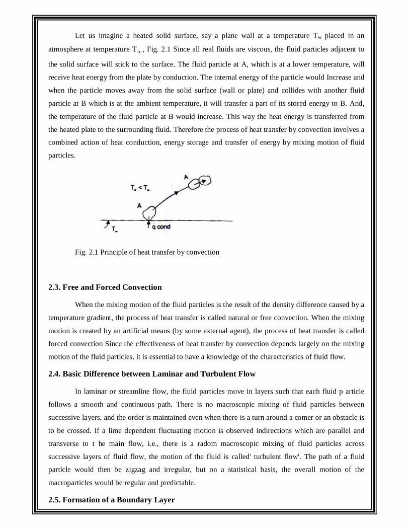
Let us imagine a heated solid surface, say a plane wall at a temperature Tw placed in an
atmosphere at temperature T , Fig. 2.1 Since all real fluids are viscous, the fluid particles adjacent to
the solid surface will stick to the surface. The fluid particle at A, which is at a lower temperature, will
receive heat energy from the plate by conduction. The internal energy of the particle would Increase and
when the particle moves away from the solid surface (wall or plate) and collides with another fluid
particle at B which is at the ambient temperature, it will transfer a part of its stored energy to B. And,
the temperature of the fluid particle at B would increase. This way the heat energy is transferred from
the heated plate to the surrounding fluid. Therefore the process of heat transfer by convection involves a
combined action of heat conduction, energy storage and transfer of energy by mixing motion of fluid
particles.
Fig. 2.1 Principle of heat transfer by convection
2.3. Free and Forced Convection
When the mixing motion of the fluid particles is the result of the density difference caused by a
temperature gradient, the process of heat transfer is called natural or free convection. When the mixing
motion is created by an artificial means (by some external agent), the process of heat transfer is called
forced convection Since the effectiveness of heat transfer by convection depends largely on the mixing
motion of the fluid particles, it is essential to have a knowledge of the characteristics of fluid flow.
2.4. Basic Difference between Laminar and Turbulent Flow
In laminar or streamline flow, the fluid particles move in layers such that each fluid p article
follows a smooth and continuous path. There is no macroscopic mixing of fluid particles between
successive layers, and the order is maintained even when there is a turn around a comer or an obstacle is
to be crossed. If a lime dependent fluctuating motion is observed indirections which are parallel and
transverse to t he main flow, i.e., there is a radom macroscopic mixing of fluid particles across
successive layers of fluid flow, the motion of the fluid is called' turbulent flow'. The path of a fluid
particle would then be zigzag and irregular, but on a statistical basis, the overall motion of the
macroparticles would be regular and predictable.
2.5. Formation of a Boundary Layer
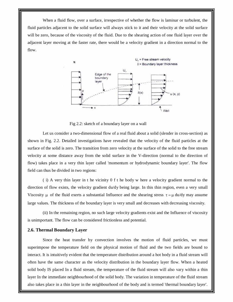
When a fluid flow, over a surface, irrespective of whether the flow is laminar or turbulent, the
fluid particles adjacent to the solid surface will always stick to it and their velocity at the solid surface
will be zero, because of the viscosity of the fluid. Due to the shearing action of one fluid layer over the
adjacent layer moving at the faster rate, there would be a velocity gradient in a direction normal to the
flow.
Fig 2.2: sketch of a boundary layer on a wall
Let us consider a two-dimensional flow of a real fluid about a solid (slender in cross-section) as
shown in Fig. 2.2. Detailed investigations have revealed that the velocity of the fluid particles at the
surface of the solid is zero. The transition from zero velocity at the surface of the solid to the free stream
velocity at some distance away from the solid surface in the V-direction (normal to the direction of
flow) takes place in a very thin layer called 'momentum or hydrodynamic boundary layer'. The flow
field can thus be divided in two regions:
( i) A very thin layer in t he vicinity 0 f t he body w here a velocity gradient normal to the
direction of flow exists, the velocity gradient du/dy being large. In this thin region, even a very small
Viscosity of the fluid exerts a substantial Influence and the shearing stress du/dy may assume
large values. The thickness of the boundary layer is very small and decreases with decreasing viscosity.
(ii) In the remaining region, no such large velocity gradients exist and the Influence of viscosity
is unimportant. The flow can be considered frictionless and potential.
2.6. Thermal Boundary Layer
Since the heat transfer by convection involves the motion of fluid particles, we must
superimpose the temperature field on the physical motion of fluid and the two fields are bound to
interact. It is intuitively evident that the temperature distribution around a hot body in a fluid stream will
often have the same character as the velocity distribution in the boundary layer flow. When a heated
solid body IS placed In a fluid stream, the temperature of the fluid stream will also vary within a thin
layer In the immediate neighbourhood of the solid body. The variation in temperature of the fluid stream
also takes place in a thin layer in the neighbourhood of the body and is termed 'thermal boundary layer'.
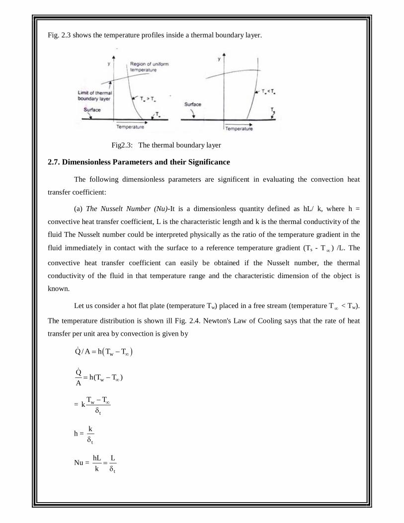
Fig. 2.3 shows the temperature profiles inside a thermal boundary layer.
Fig2.3: The thermal boundary layer
2.7. Dimensionless Parameters and their Significance
The following dimensionless parameters are significent in evaluating the convection heat
transfer coefficient:
(a) The Nusselt Number (Nu)-It is a dimensionless quantity defined as hL/ k, where h =
convective heat transfer coefficient, L is the characteristic length and k is the thermal conductivity of the
fluid The Nusselt number could be interpreted physically as the ratio of the temperature gradient in the
fluid immediately in contact with the surface to a reference temperature gradient (Ts - T ) /L. The
convective heat transfer coefficient can easily be obtained if the Nusselt number, the thermal
conductivity of the fluid in that temperature range and the characteristic dimension of the object is
known.
Let us consider a hot flat plate (temperature Tw) placed in a free stream (temperature T < Tw).
The temperature distribution is shown ill Fig. 2.4. Newton's Law of Cooling says that the rate of heat
transfer per unit area by convection is given by
wQ/ A h T T
wQ h(T T )A
= w
t
T Tk
h = t
k
Nu = t
hL Lk
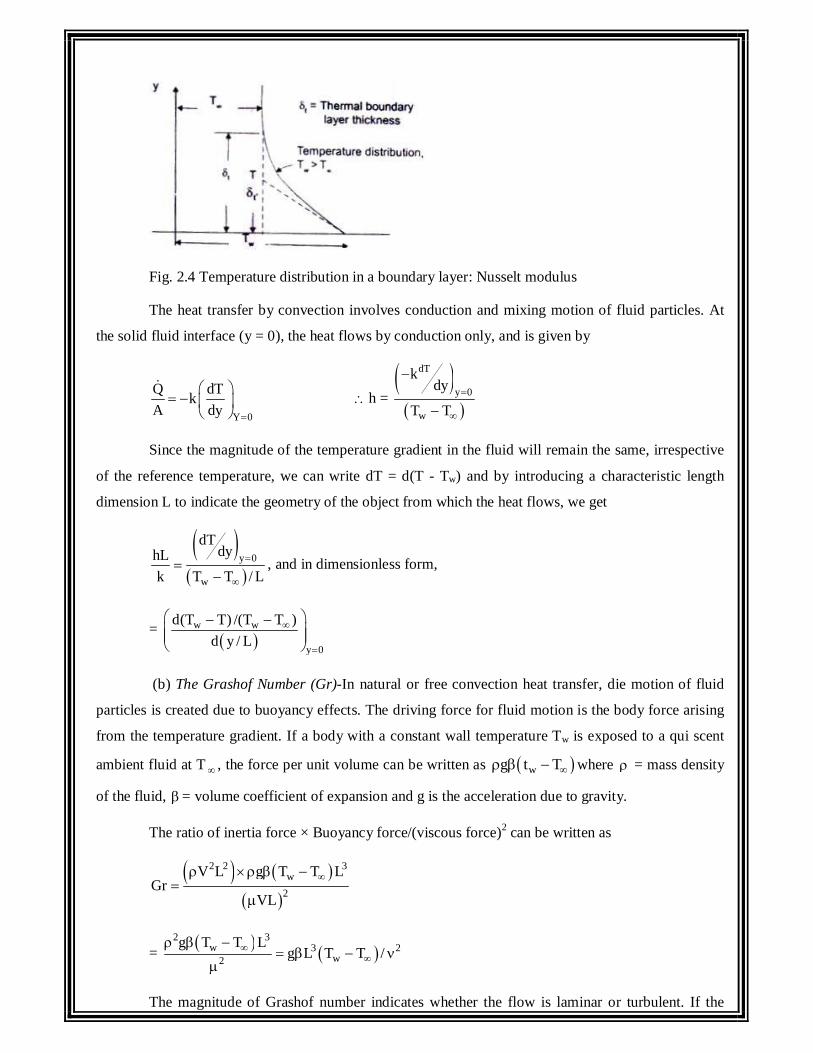
Fig. 2.4 Temperature distribution in a boundary layer: Nusselt modulus
The heat transfer by convection involves conduction and mixing motion of fluid particles. At
the solid fluid interface (y = 0), the heat flows by conduction only, and is given by
Y 0
Q dTkA dy
h =
dT
y 0
w
kdy
T T
Since the magnitude of the temperature gradient in the fluid will remain the same, irrespective
of the reference temperature, we can write dT = d(T - Tw) and by introducing a characteristic length
dimension L to indicate the geometry of the object from which the heat flows, we get
y 0
w
dTdyhL
k T T / L
, and in dimensionless form,
=
w w
y 0
d(T T) /(T T )d y / L
(b) The Grashof Number (Gr)-In natural or free convection heat transfer, die motion of fluid
particles is created due to buoyancy effects. The driving force for fluid motion is the body force arising
from the temperature gradient. If a body with a constant wall temperature Tw is exposed to a qui scent
ambient fluid at T , the force per unit volume can be written as wg t T where = mass density
of the fluid, = volume coefficient of expansion and g is the acceleration due to gravity.
The ratio of inertia force × Buoyancy force/(viscous force)2 can be written as
2 2 3w
2
V L g T T LGr
VL
= 2 3
w 3 2w2
g T T Lg L T T /
The magnitude of Grashof number indicates whether the flow is laminar or turbulent. If the
Grashof number is greater than 109, the flow is turbulent and for Grashof number less than 108, the flow
is laminar. For 108 < Gr < 109, It is the transition range.
(c) The Prandtl Number (Pr) - It is a dimensionless parameter defined as
Pr = pC / k /
where is the dynamic viscosity of the fluid, v = kinematic viscosity and = thermal
diffusivity.
This number assumes significance when both momentum and energy are propagated through
the system. It is a physical parameter depending upon the properties of the medium It is a measure of the
relative magnitudes of momentum and thermal diffusion in the fluid: That is, for Pr = I, the r ate of
diffusion of momentum and energy are equal which means that t he calculated temperature and velocity
fields will be Similar, the thickness of the momentum and thermal boundary layers will be equal. For Pr
<<I (in case of liquid metals), the thickness of the thermal boundary layer will be much more than the
thickness of the momentum boundary layer and vice versa. The product of Grashof and Prandtl number
is called Rayleigh number. Or, Ra = Gr × Pr.
2.8. Evaluation of Convective Heat Transfer Coefficient
The convective heat transfer coefficient in free or natural convection can be evaluated by two
methods:
(a) Dimensional Analysis combined with experimental investigations
(b) Analytical solution of momentum and energy equations 10 the boundary layer.
Dimensional Analysis and Its Limitations
Since the evaluation of convective heat transfer coefficient is quite complex, it is based on a
combination of physical analysis and experimental studies. Experimental observations become
necessary to study the influence of pertinent variables on the physical phenomena.
Dimensional analysis is a mathematical technique used in reducing the number of experiments
to a minimum by determining an empirical relation connecting the relevant variables and in grouping
the variables together in terms of dimensionless numbers. And, the method can only be applied after the
pertinent variables controlling t he phenomenon are Identified and expressed In terms of the primary
dimensions. (Table 1.1)
In natural convection heat transfer, the pertinent variables are: h, , k, , Cp, L, ( T), and
g. Buckingham 's method provides a systematic technique for arranging the variables in dimensionless
numbers. It states that the number of dimensionless groups, ’s, required to describe a phenomenon
involving 'n' variables is equal to the number of variables minus the number of primary dimensions 'm'
in the problem.
In SI system of units, the number of primary dimensions are 4 and the number of variables for
free convection heat transfer phenomenon are 9 and therefore, we should expect (9 - 4) = 5
dimensionless numbers. Since the dimension of the coefficient of volume expansion, , is 1 , one
dimensionless number is obviously (T). The remaining variables are written in a functional form:
ph, ,k, ,C ,L,g = 0.
Since the number of primary dimensions are 4, we arbitrarily choose 4 independent variables as
primary variables such that all the four dimensions are represented. The selected primary variables are:
,g, k. L Thus the dimensionless group,
a ba b c d 3 2 3 1 0 0 0 01 g k L h ML LT . MLT M L T
Equating the powers of M, L, T, on both sides, we have
M : a + c + 1 = 0 } Upon solving them, L : -3a + b + c + d = 0 T : -2b -3c -3 = 0 : -c - 1 = 0
Up on solving them,
c = 1, b = a = 0 and d = 1.
and 1 = hL/k, the Nusselt number.
The other dimensionless number
2= pagbkcLdCp = (ML-3)a (LT-2)b(MLT-3 -1)c(L)d(MT-1 1 ) = M0L0T0 0 Equating the powers
of M,L,T and and upon solving, we get
3= 2 2 3/ gL
By combining 2 and 3 , we write 1/ 24 2 3
= 1/ 22 3 2 2 2 3
pgL C / k / gL = pCk
(the Prandtl number)
By combining 3 with T , we have 5= T *3
1
= 2 3
3 22
gLT g T L /
(the Grashof number)
Therefore, the functional relationship is expressed as:
m1Nu,Pr,Gr 0;Or, Nu Gr Pr Const Gr Pr (2.1)
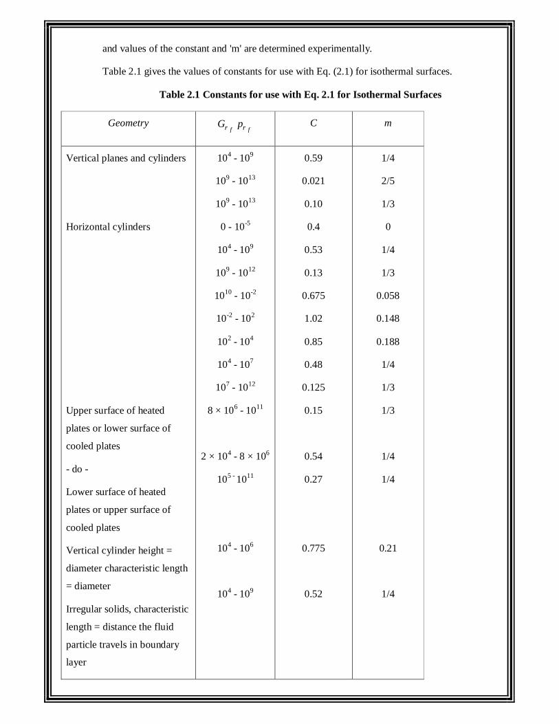
and values of the constant and 'm' are determined experimentally.
Table 2.1 gives the values of constants for use with Eq. (2.1) for isothermal surfaces.
Table 2.1 Constants for use with Eq. 2.1 for Isothermal Surfaces
Geometry f fr rG p C m
Vertical planes and cylinders
Horizontal cylinders
Upper surface of heated
plates or lower surface of
cooled plates
- do -
Lower surface of heated
plates or upper surface of
cooled plates
Vertical cylinder height =
diameter characteristic length
= diameter
Irregular solids, characteristic
length = distance the fluid
particle travels in boundary
layer
104 - 109
109 - 1013
109 - 1013
0 - 10-5
104 - 109
109 - 1012
1010 - 10-2
10-2 - 102
102 - 104
104 - 107
107 - 1012
8 × 10⁶ - 1011
2 × 10⁴ - 8 × 10⁶
105 - 1011
104 - 106
104 - 109
0.59
0.021
0.10
0.4
0.53
0.13
0.675
1.02
0.85
0.48
0.125
0.15
0.54
0.27
0.775
0.52
1/4
2/5
1/3
0
1/4
1/3
0.058
0.148
0.188
1/4
1/3
1/3
1/4
1/4
0.21
1/4
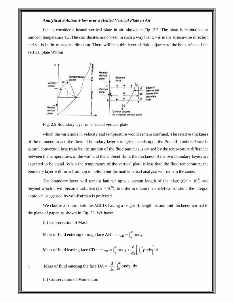
Analytical Solution-Flow over a Heated Vertical Plate in Air
Let us consider a heated vertical plate in air, shown in Fig. 2.5. The plate is maintained at
uniform temperature Tw .The coordinates are chosen in such a way that x - is in the streamwise direction
and y - is in the transverse direction. There will be a thin layer of fluid adjacent to the hot surface of the
vertical plate Within
Fig. 2.5 Boundary layer on a heated vertical plate
which the variations in velocity and temperature would remain confined. The relative thickness
of the momentum and the thermal boundary layer strongly depends upon the Prandtl number. Since in
natural convection heat transfer, the motion of the fluid particles is caused by the temperature difference
between the temperatures of the wall and the ambient fluid, the thickness of the two boundary layers are
expected to be equal. When the temperature of the vertical plate is less than the fluid temperature, the
boundary layer will form from top to bottom but the mathematical analysis will remain the same.
The boundary layer will remain laminar upto a certain length of the plate (Gr < 108) and
beyond which it will become turbulent (Gr > 109). In order to obtain the analytical solution, the integral
approach, suggested by von-Karman is preferred.
We choose a control volume ABCD, having a height H, length dx and unit thickness normal to
the plane of paper, as shown in Fig. 25. We have:
(b) Conservation of Mass:
Mass of fluid entering through face AB = H
AB 0m udy
Mass of fluid leaving face CD = H H
CD 0 0
dm udy udy dxdx
Mass of fluid entering the face DA = H
0
d udy dxdx
(ii) Conservation of Momentum :
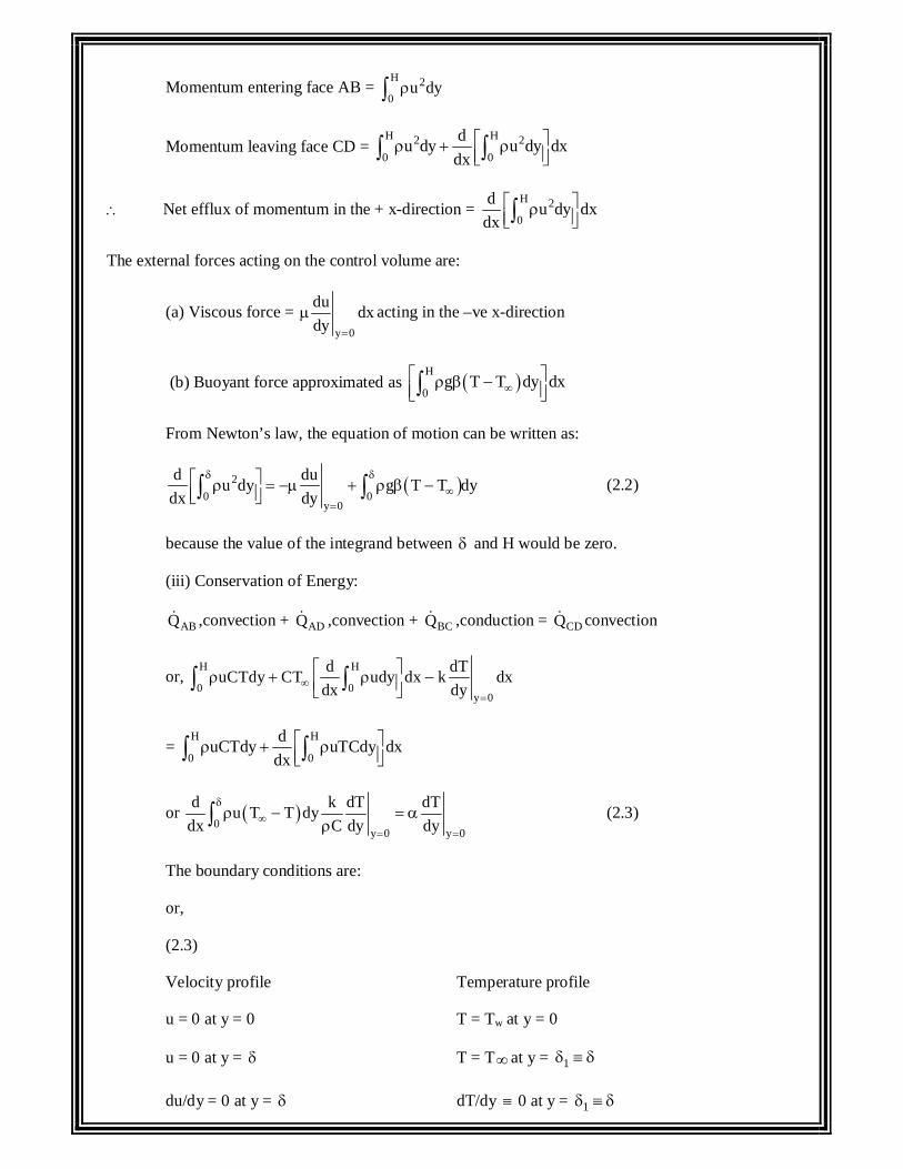
Momentum entering face AB = H 20
u dy
Momentum leaving face CD = H H2 20 0
du dy u dy dxdx
Net efflux of momentum in the + x-direction = H 20
d u dy dxdx
The external forces acting on the control volume are:
(a) Viscous force = y 0
du dxdy
acting in the –ve x-direction
(b) Buoyant force approximated as H
0g T T dy dx
From Newton’s law, the equation of motion can be written as:
20 0
y 0
d duu dy g T T dydx dy
(2.2)
because the value of the integrand between and H would be zero.
(iii) Conservation of Energy:
ABQ ,convection + ADQ ,convection + BCQ ,conduction = CDQ convection
or, H H
0 0y 0
d dTuCTdy CT udy dx k dxdx dy
= H H
0 0
duCTdy uTCdy dxdx
or 0
y 0 y 0
d k dT dTu T T dydx C dy dy
(2.3)
The boundary conditions are:
or,
(2.3)
Velocity profile Temperature profile
u = 0 at y = 0 T = Tw at y = 0
u = 0 at y = T = T at y = 1
du/dy = 0 at y = dT/dy 0 at y = 1
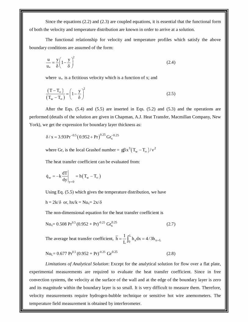
Since the equations (2.2) and (2.3) are coupled equations, it is essential that the functional form
of both the velocity and temperature distribution are known in order to arrive at a solution.
The functional relationship for velocity and temperature profiles which satisfy the above
boundary conditions are assumed of the form:
2
*
u y y1u
(2.4)
where *u is a fictitious velocity which is a function of x; and
2
w
T T y1T T
(2.5)
After the Eqs. (5.4) and (5.5) are inserted in Eqs. (5.2) and (5.3) and the operations are
performed (details of the solution are given in Chapman, A.J. Heat Transfer, Macmillan Company, New
York), we get the expression for boundary layer thickness as:
0.250.5 0.25x/ x 3.93Pr 0.952 Pr Gr
where Gr, is the local Grashof number = 3 2wg x T T /
The heat transfer coefficient can be evaluated from:
w wy 0
dTq k h T Tdy
Using Eq. (5.5) which gives the temperature distribution, we have
h = 2k/ or, hx/k = Nux= 2x/
The non-dimensional equation for the heat transfer coefficient is
Nux= 0.508 Pr0.5 (0.952 + Pr)-0.25 0.25xGr (2.7)
The average heat transfer coefficient, L
x x L0
1h h dx 4 /3hL
NuL= 0.677 Pr0.5 (0.952 + Pr)-0.25 0.25Gr (2.8)
Limitations of Analytical Solution: Except for the analytical solution for flow over a flat plate,
experimental measurements are required to evaluate the heat transfer coefficient. Since in free
convection systems, the velocity at the surface of the wall and at the edge of the boundary layer is zero
and its magnitude within the boundary layer is so small. It is very difficult to measure them. Therefore,
velocity measurements require hydrogen-bubble technique or sensitive hot wire anemometers. The
temperature field measurement is obtained by interferometer.
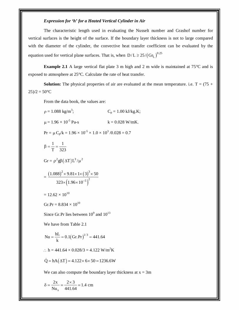
Expression for ‘h’ for a Heated Vertical Cylinder in Air
The characteristic length used in evaluating the Nusselt number and Grashof number for
vertical surfaces is the height of the surface. If the boundary layer thickness is not to large compared
with the diameter of the cylinder, the convective heat transfer coefficient can be evaluated by the
equation used for vertical plane surfaces. That is, when 0.25LD / L 25/ Gr
Example 2.1 A large vertical flat plate 3 m high and 2 m wide is maintained at 75°C and is
exposed to atmosphere at 25°C. Calculate the rate of heat transfer.
Solution: The physical properties of air are evaluated at the mean temperature. i.e. T = (75 +
25)/2 = 50°C
From the data book, the values are:
= 1.088 kg/m3; Cp = 1.00 kJ/kg.K;
= 1.96 × 10⁻⁵ Pa-s k = 0.028 W/mK.
Pr = Cp/k = 1.96 × 10-5 × 1.0 × 103 /0.028 = 0.7
1 1T 323
Gr = 2 3 2g T L /
=
2 3
25
1.088 9.81 1 3 50
323 1.96 10
= 12.62 × 10¹⁰
Gr.Pr = 8.834 × 10¹⁰
Since Gr.Pr lies between 109 and 1013
We have from Table 2.1
1/ 3hLNu 0.1 Gr.Pr 441.64k
h = 441.64 × 0.028/3 = 4.122 W/m2K
Q hA T 4.122 6 50 1236.6W
We can also compute the boundary layer thickness at x = 3m
x
2x 2 3 1.4 cmNu 441.64
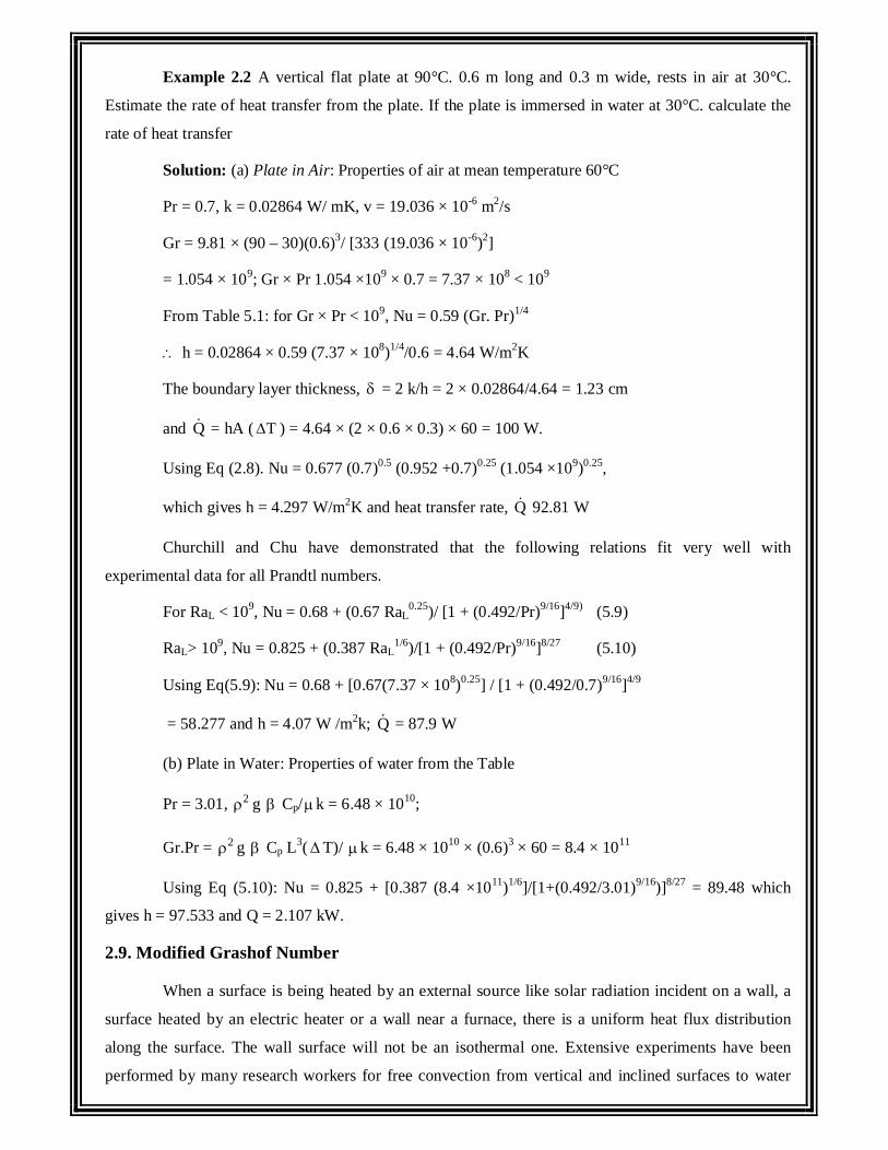
Example 2.2 A vertical flat plate at 90°C. 0.6 m long and 0.3 m wide, rests in air at 30°C.
Estimate the rate of heat transfer from the plate. If the plate is immersed in water at 30°C. calculate the
rate of heat transfer
Solution: (a) Plate in Air: Properties of air at mean temperature 60°C
Pr = 0.7, k = 0.02864 W/ mK, v = 19.036 × 10⁻⁶ m2/s
Gr = 9.81 × (90 – 30)(0.6)3/ [333 (19.036 × 10⁻⁶)2]
= 1.054 × 10⁹; Gr × Pr 1.054 ×109 × 0.7 = 7.37 × 10⁸ < 109
From Table 5.1: for Gr × Pr < 109, Nu = 0.59 (Gr. Pr)1/4
h = 0.02864 × 0.59 (7.37 × 10⁸)1/4/0.6 = 4.64 W/m2K
The boundary layer thickness, = 2 k/h = 2 × 0.02864/4.64 = 1.23 cm
and Q = hA ( T ) = 4.64 × (2 × 0.6 × 0.3) × 60 = 100 W.
Using Eq (2.8). Nu = 0.677 (0.7)0.5 (0.952 +0.7)0.25 (1.054 ×10⁹)0.25,
which gives h = 4.297 W/m2K and heat transfer rate, Q 92.81 W
Churchill and Chu have demonstrated that the following relations fit very well with
experimental data for all Prandtl numbers.
For RaL < 109, Nu = 0.68 + (0.67 RaL0.25)/ [1 + (0.492/Pr)9/16]4/9) (5.9)
RaL> 109, Nu = 0.825 + (0.387 RaL1/6)/[1 + (0.492/Pr)9/16]8/27 (5.10)
Using Eq(5.9): Nu = 0.68 + [0.67(7.37 × 10⁸)0.25] / [1 + (0.492/0.7)9/16]4/9
= 58.277 and h = 4.07 W /m2k; Q = 87.9 W
(b) Plate in Water: Properties of water from the Table
Pr = 3.01, 2 g Cp/k = 6.48 × 10¹⁰;
Gr.Pr = 2 g Cp L3(T)/ k = 6.48 × 1010 × (0.6)3 × 60 = 8.4 × 10¹¹
Using Eq (5.10): Nu = 0.825 + [0.387 (8.4 ×10¹¹)1/6]/[1+(0.492/3.01)9/16)]8/27 = 89.48 which
gives h = 97.533 and Q = 2.107 kW.
2.9. Modified Grashof Number
When a surface is being heated by an external source like solar radiation incident on a wall, a
surface heated by an electric heater or a wall near a furnace, there is a uniform heat flux distribution
along the surface. The wall surface will not be an isothermal one. Extensive experiments have been
performed by many research workers for free convection from vertical and inclined surfaces to water
under constant heat flux conditions. Since the temperature difference ( T) is not known beforehand,
the Grashof number is modified by multiplying it by Nusselt number. That is,
*xGr = Grx. Nux = (g T / 2 ) × (hx/k) = g x4 q/k 2 (2.11)
where q is the wall heat flux in Wm2. (q = h ( T ))
It has been observed that the boundary layer remains lam mar when the modified Rayleigh
number, Ra* = *xGr ’. Pr is less than 3 × 10¹² and fully turbulent flow appears for Ra* > 1014. The local
heat transfer coefficient can be calculated from:
q constant and 105 < *xGr <1011: Nux = 0.60 ( *
xGr . Pr)0.2 (2.12)
q constant and 2 × 10¹³< *xGr < 1016 : Nux= 0.17 ( *
xGr . Pr)0.25 (2.13)
Although these results are based on experiments for water, they are applicable to air as well.
The physical properties are to be evaluated at the local film temperature.
Example 2.3 Solar radiation of intensity 700W/m’ is incident on a vertical wall, 3 m high and
3 m wide. Assuming that the wall does not transfer energy to the inside surface and all the incident
energy is lost by free convection to the ambient air at 30oe, calculate the average temperature of the
wall
Solution: Since the surface temperature of the wall is not known, we assume a value for h = 7
W/m2 K.
T = q / h = 700/7 = 100oC and the film temperature = (30 + 130) /2 = 80oC
The properties of air at 273 +80 = 353 are : = 1/353, Pr = 0.697
k = 0.03 W /mK, = 20.76 ×10⁻⁶ m2/s.
Modified Grashof number, *xGr = 9.81 . (1/353)· (3)4 × 700/[0.03 ×(20.76 × 10-6 )2] = 1.15 × 10¹⁴
From Eq. (2.13), h = (k/x) (0.17) ( *xGr Pr)0.25
= (0.03/3 )(0.17)( 1.15 × 1014 × 0.697)1/4
= 5.087 W/m2K, a different value from the assumed value.
Second Trial: T = q / h = 700/5.087 = 137.66 and film temperature
= 98.8°C
The properties of air at (273 + 98.8) °C are: =1/372, k = 0.0318 W/mK
Pr = 0.693, v = 23.3 × 10⁻⁶ m2/s
*xGr = 9.81 . (1/372)· (3)4 × 700/[0.318(23.3 × 10-6)2] = 8.6 × 10¹³
Using Eq (2.13), h = (k/x)(0.17)( *xGr Pr)1/4 = 5.015 W/m2k, an acceptable value. In 67urbulent
heat transfer by convection, Eq. (5.13) tells us that the local heat transfer coefficient hx does not vary
with x and therefore, the average and local heat transfer coefficients are the same.
2 Laminar Flow Forced Convection Heat Transfer
2.1Forced Convection Heat Transfer Principles
The mechanism of heat transfer by convection requires mixing of one portion of fluid with
another portion due to gross movement of the mass of the fluid. The transfer of heat energy from one
fluid particle or a molecule to another one is still by conduction but the energy is transported from one
point in space to another by the displacement of fluid.
When the motion of fluid is created by the imposition of external forces in the form of pressure
differences, the process of heat transfer is called ‘forced convection’. And, the motion of fluid particles
may be either laminar or turbulent and that depends upon the relative magnitude of inertia and viscous
forces, determined by the dimensionless parameter Reynolds number. In free convection, the velocity of
fluid particle is very small in comparison with the velocity of fluid particles in forced convection,
whether laminar or turbulent. In forced convection heat transfer, Gr/Re2<< 1, in free convection heat
transfer, GrRe2>>1 and we have combined free and forced convection when Gr/Re2 1 .
2.2. Methods for Determining Heat Transfer Coefficient
The convective heat transfer coefficient in forced flow can be evaluated by: (a)
Dimensional Analysis combined with experiments;
(b) Reynolds Analogy – an analogy between heat and momentum transfer; (c) Analytical
Methods – exact and approximate analyses of boundary layer
equations.
2.3. Method of Dimensional Analysis
As pointed out in Chapter 5, dimensional analysis does not yield equations which can be
solved. It simply combines the pertinent variables into non-dimensional numbers which facilitate the
interpretation and extend the range of application of experimental data. The relevant variables for forced
convection heat transfer phenomenon whether laminar or turbulent, are
(b) the properties of the fluid – density p, specific heat capacity Cp, dynamic or absolute
viscosity , thermal conductivity k.
(ii) the properties of flow – flow velocity Y, and the characteristic dimension of the system L.
As such, the convective heat transfer coefficient, h, is written as h = f ( , V, L, , Cp, k) = 0
(5.14)
Since there are seven variables and four primary dimensions, we would expect three
dimensionless numbers. As before, we choose four independent or core variables as ,V, L, k, and
calculate the dimensionless numbers by applying Buckingham ’s method:
1 = a b dca b c d 3 1 3 1 3 1V L K h ML LT L MLT MT
= o o o oM L T
Equating the powers of M, L, T and on both sides, we get
M : a + d + 1 = O
L : - 3a + b + c + d = 0
T : - b – 3d – 3 = 0 By solving them, we have
: - d – 1= 0. D = -1, a = 0, b = 0, c = 1.
Therefore, 1 = hL/k is the Nusselt number.
2 = a b dca b c d 3 1 3 1 1 1V L K ML LT L MLT ML T
= o o o oM L T
Equating the powers of M, L, T and on both sides, we get
M : a + d +1 = 0
L : - 3a + b + c + d = 1 = 0
T : - b – 3d – 1 = 0
: - d = 0.
By solving them, d = 0, b = - 1, a = - 1, c = - 1
and 2 32
1 VL/ VL;or,
(Reynolds number is a flow parameter of greatest significance. It is the ratio of inertia forces to
viscous forces and is of prime importance to ascertain the conditions under which a flow is laminar or
turbulent. It also compares one flow with another provided the corresponding length and velocities are
comparable in two flows. There would be a similarity in flow between two flows when the Reynolds
numbers are equal and the geometrical similarities are taken into consideration.)
a b dca b c d 3 1 3 1 2 2 14 pV L k C ML LT L MLT L T
o o o oM L T
Equating the powers of M, L, T, on both Sides, we get
M : a + d = 0; L : - 3a + b + c + d + 2 = 0
T : - b – 3d – 2 = 0; : - d – 1 = 0
By solving them,
d =- 1,a = l, b = l, c = l,
4 p 5 4 2VL C ; k
pp
CVL C =k VL k
5 is Prandtl number.
Therefore, the functional relationship is expressed as:
Nu = f (Re, Pr); or Nu = C Rem Prn (5.15)
where the values of c, m and n are determined experimentally.
2.4. Principles of Reynolds Analogy
Reynolds was the first person to observe that there exists a similarity between the exchange of
momentum and the exchange of heat energy in laminar motion and for that reason it has been termed
‘Reynolds analogy’. Let us consider the motion of a fluid where the fluid is flowing over a plane wall.
The X-coordinate is measured parallel to the surface and the V-coordinate is measured normal to it.
Since all fluids are real and viscous, there would be a thin layer, called momentum boundary layer, in
the vicinity of the wall where a velocity gradient normal to the direction of flow exists. When the
temperature of the surface of the wall is different than the temperature of the fluid stream, there would
also be a thin layer, called thermal boundary layer, where there is a variation in temperature normal to
the direction of flow. Fig. 2.6 depicts the velocity distribution and temperature profile for the laminar
motion of the fluid flowing past a plane wall.
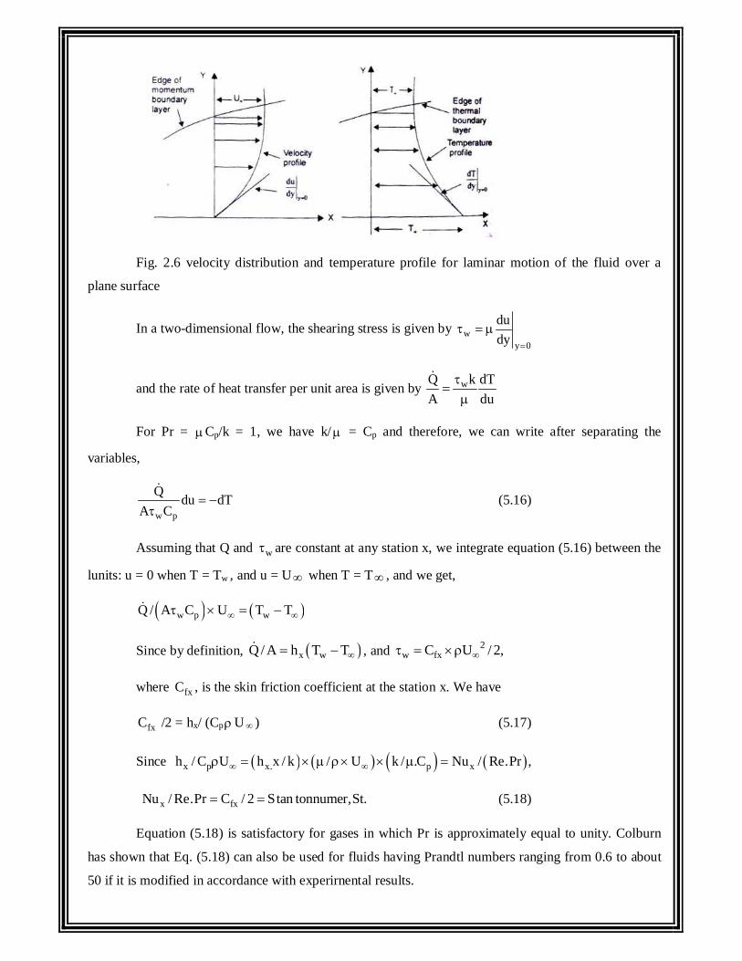
Fig. 2.6 velocity distribution and temperature profile for laminar motion of the fluid over a
plane surface
In a two-dimensional flow, the shearing stress is given by wy 0
dudy
and the rate of heat transfer per unit area is given by wkQ dTA du
For Pr = Cp/k = 1, we have k/ = Cp and therefore, we can write after separating the
variables,
w p
Q du dTA C
(5.16)
Assuming that Q and w are constant at any station x, we integrate equation (5.16) between the
lunits: u = 0 when T = Tw , and u = U when T = T , and we get,
w p wQ / A C U T T
Since by definition, x wQ/ A h T T , and 2w fxC U / 2,
where fxC , is the skin friction coefficient at the station x. We have
fxC /2 = hx/ (CpU ) (5.17)
Since x p x. p xh / C U h x / k / U k / .C Nu / Re.Pr ,
x fxNu / Re.Pr C / 2 Stan tonnumer,St. (5.18)
Equation (5.18) is satisfactory for gases in which Pr is approximately equal to unity. Colburn
has shown that Eq. (5.18) can also be used for fluids having Prandtl numbers ranging from 0.6 to about
50 if it is modified in accordance with experirnental results.
Or, 2 / 3 2/ 3xx fx
x
Nu .Pr St Pr C / 2Re Pr
(5.19)
Eq. (5.19) expresses the relation between fluid friction and heat transfer for laminar flow over a
plane wall. The heat transfer coefficient could thus be determined by making measurements of the
frictional drag on a plate under conditions in which no heat transfer is involved.
Example 2.4 Glycerine at 35°C flows over a 30cm by 3Ocm flat plate at a velocity of 1.25 m/s.
The drag force is measured as 9.8 N (both Side of the plate). Calculate the heat transfer for such a flow
system.
Solution: From tables, the properties of glycerine at 35°C are:
= 1256 kg/m3, Cp = 2.5 kJ/kgK, = 0.28 kg/m-s, k = 0.286 W/mK, Pr = 2.4 Re= VL/ =
1256 × 1.25 × 0.30/0.28 = 1682.14, a laminar flow.*
Average shear stress on one side of the plate = drag force/area
= 9.8/(2 × 0.3 × 0.3) = 54.4
and shear stress = C f U2/2
The average skin friction coefficient, Cr/ 2 = 2U
= 54.4/( 1256 ×1.25 × 1.25) = 0.0277
From Reynolds analogy, Cf /2 = St. Pr 2/3
or, h = Cp U × Cf/2 × Pr -2/3 = 0.667
1256 2.5 1.25 0.02772.45
=59.8 kW/m2K.
2.5. Analytical Evaluation of ‘h’ for Laminar Flow over a Flat Plat – Assumptions
As pointed out earlier, when the motion of the fluid is caused by the imposition of external
forces, such as pressure differences, and the fluid flows over a solid surface, at a temperature different
from the temperature of the fluid, the mechanism of heat transfer is called ‘forced convection’.
Therefore, any analytical approach to determine the convective heat transfer coefficient would require
the temperature distribution in the flow field surrounding the body. That is, the theoretical analysis
would require the use of the equation of motion of the viscous fluid flowing over the body along with
the application of the principles of conservation of mass and energy in order to relate the heat energy
that is convected away by the fluid from the solid surface.
For the sake of simplicity, we will consider the motion of the fluid in 2 space dimension, and a
steady flow. Further, the fluid properties like viscosity, density, specific heat, etc are constant in the
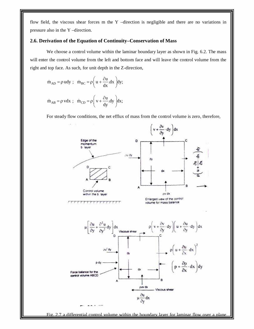
flow field, the viscous shear forces m the Y –direction is negligible and there are no variations in
pressure also in the Y –direction.
2.6. Derivation of the Equation of Continuity–Conservation of Mass
We choose a control volume within the laminar boundary layer as shown in Fig. 6.2. The mass
will enter the control volume from the left and bottom face and will leave the control volume from the
right and top face. As such, for unit depth in the Z-direction,
AD BCum udy ; m u .dx dy;
dx
AB CDum vdx ; m v .dy dx;
dy
For steady flow conditions, the net efflux of mass from the control volume is zero, therefore,
Fig. 2.7 a differential control volume within the boundary layer for laminar flow over a plane
wall
u vudy xdx udy dxdy vdx .dxdyx x
or, u / x v y 0, the equation of continuity. (2.20)
Concept of Critical Thickness of Insulation
The addition of insulation at the outside surface of small pipes may not reduce the rate of heat
transfer. When an insulation is added on the outer surface of a bare pipe, its outer radius, r0 increases
and this increases the thermal resistance due to conduction logarithmically whereas t he thermal
resistance to heat flow due to fluid film on the outer surface decreases linearly with increasing radius, r0.
Since the total thermal resistance is proportional to the sum of these two resistances, the rate of heat
flow may not decrease as insulation is added to the bare pipe.
Fig. 2.7 shows a plot of heat loss against the insulation radius for two different cases. For small
pipes or wires, the radius rl may be less than re and in that case, addition of insulation to the bare pipe
will increase the heat loss until the critical radius is reached. Further addition of insulation will decrease
the heat loss rate from this peak value. The insulation thickness (r* – rl) must be added to reduce the
heat loss below the uninsulated rate. If the outer pipe radius rl is greater than the critical radius re any
insulation added will decrease the heat loss.
2.7 Expression for Critical Thickness of Insulation for a Cylindrical Pipe
Let us consider a pipe, outer radius rl as shown in Fig. 2.18. An insulation is added such that
the outermost radius is r a variable and the insulation thickness is
(r – rI). We assume that the thermal conductivity, k, for the insulating material is very small in
comparison with the thermal conductivity of the pipe material and as such the temperature T1, at the
inside surface of the insulation is constant. It is further assumed that both h and k are constant. The rate
of heat flow, per unit length of pipe, through the insulation is then,
1 1Q / L 2 T T / ln r / r / k 1/ hr , where T is the ambient temperature.
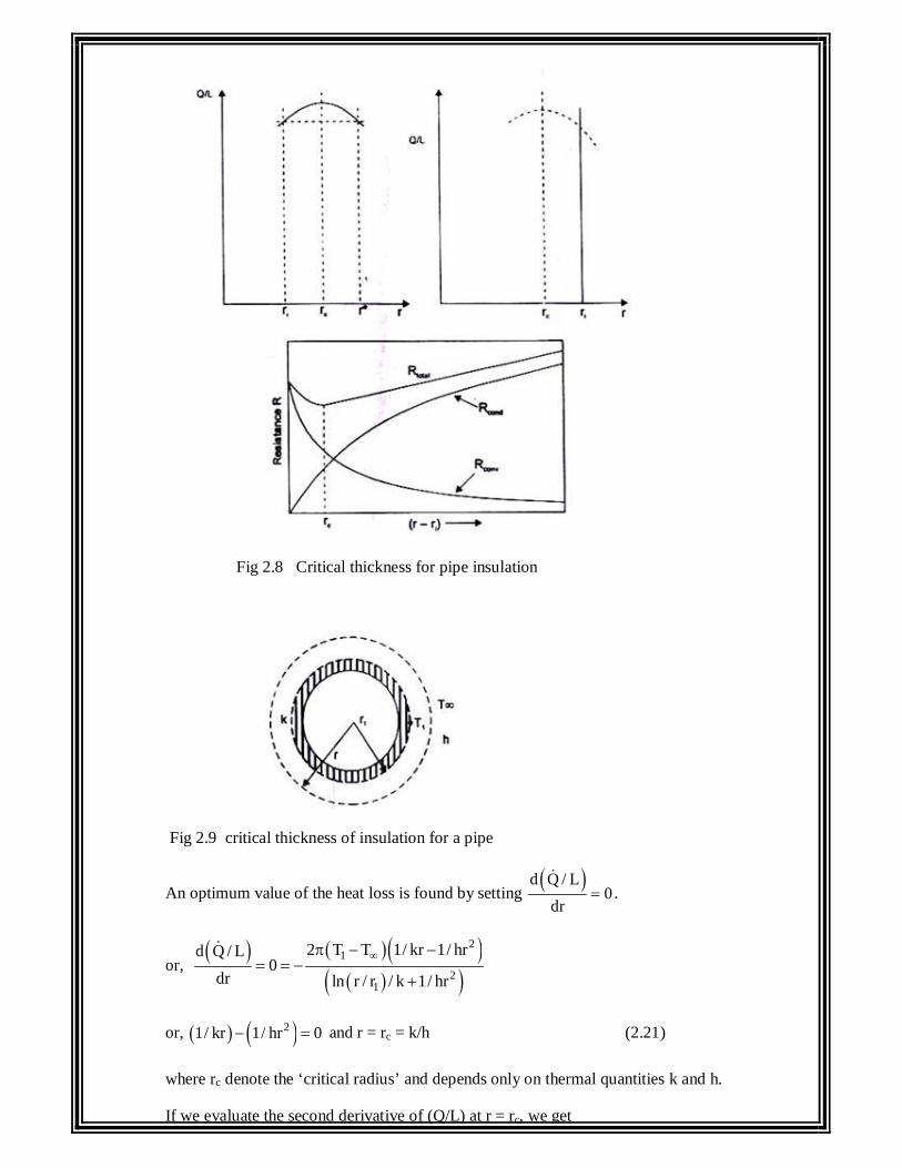
Fig 2.8 Critical thickness for pipe insulation
Fig 2.9 critical thickness of insulation for a pipe
An optimum value of the heat loss is found by setting d Q / L
0dr
.
or,
2
1
21
2 T T 1/ kr 1/ hrd Q / L0
dr ln r / r / k 1/ hr
or, 21/ kr 1/ hr 0 and r = rc = k/h (2.21)
where rc denote the ‘critical radius’ and depends only on thermal quantities k and h.
If we evaluate the second derivative of (Q/L) at r = rc, we get
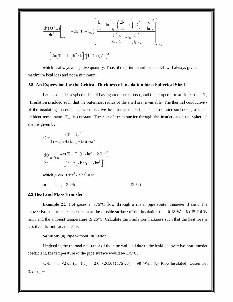
c
c
2
21
12r r
1 r r
k r 2k kIn 1 2 1d Q / L hr r hr hr
2 T Tdr 1 k rr In
kr h r
= 221 c 12 T T h / k / 1 1n r / r
which is always a negative quantity. Thus, the optimum radius, rc = k/h will always give a
maximum heal loss and not a minimum.
2.8. An Expression for the Critical Thickness of Insulation for a Spherical Shell
Let us consider a spherical shell having an outer radius r1 and the temperature at that surface T1
. Insulation is added such that the outermost radius of the shell is r, a variable. The thermal conductivity
of the insulating material, k, the convective heat transfer coefficient at the outer surface, h, and the
ambient temperature T is constant. The rate of heat transfer through the insulation on the spherical
shell is given by
12
1 1
T TQ
r r / 4 k r r 1/ h 4 r
2 31
221 1
4 T T 1/ kr 2 / hrdQ 0dr r r / k r r 1/ hr
which gives, 1/Kr2 - 2/hr3 = 0;
or r = rc = 2 k/h (2.22)
2.9 Heat and Mass Transfer
Example 2.5 Hot gases at 175°C flow through a metal pipe (outer diameter 8 cm). The
convective heat transfer coefficient at the outside surface of the insulation (k = 0.18 W mK) IS 2.6 W
m1K and the ambient temperature IS 25°C. Calculate the insulation thickness such that the heat loss is
less than the uninsulated case.
Solution: (a) Pipe without Insulation
Neglecting the thermal resistance of the pipe wall and due to the inside convective heat transfer
coefficient, the temperature of the pipe surface would be 175°C.
Q /L = h ×2r (T1-T ) = 2.6 ×2O.04{175-25) = 98 W/m (b) Pipe Insulated. Outermost
Radius, r*
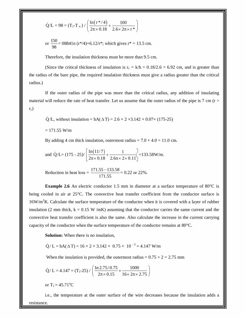
Q /L = 98 = (T1-T ) / 1n r * / 4 1002 0.18 2.6 2 r *
or 15098
= 08841n (r*/4)+6.12/r*; which gives r* = 13.5 cm.
Therefore, the insulation thickness must be more than 9.5 cm.
(Since the critical thickness of insulation is rc = k/h = 0.18/2.6 = 6.92 cm, and is greater than
the radius of the bare pipe, the required insulation thickness must give a radius greater than the critical
radius.)
If the outer radius of the pipe was more than the critical radius, any addition of insulating
material will reduce the rate of heat transfer. Let us assume that the outer radius of the pipe is 7 cm (r >
rc)
Q /L, without insulation = hA( T) = 2.6 × 2 ×3.142 × 0.07× (175-25)
= 171.55 W/m
By adding 4 cm thick insulation, outermost radius = 7.0 + 4.0 = 11.0 cm.
and Q /L= (175 - 25)/ 1n 11/ 7 12 0.18 2.6 2 0.11
=133.58W/m.
Reduction in heat loss = 171.55 133.58171.55
= 0.22 or 22%.
Example 2.6 An electric conductor 1.5 mm in diameter at a surface temperature of 80°C is
being cooled in air at 25°C. The convective heat transfer coefficient from the conductor surface is
16W/m2K. Calculate the surface temperature of the conductor when it is covered with a layer of rubber
insulation (2 mm thick, k = 0.15 W /mK) assuming that the conductor carries the same current and the
convective heat transfer coefficient is also the same. Also calculate the increase in the current carrying
capacity of the conductor when the surface temperature of the conductor remains at 80°C.
Solution: When there is no insulation,
Q / L = hA(T) = 16 × 2 × 3.142 × 0.75 × 10 - 3 = 4.147 W/m
When the insulation is provided, the outermost radius = 0.75 + 2 = 2.75 mm
Q / L = 4.147 = (T1-25) / 1n 2.75/ 0.75 10002 0.15 16 2 2.75
or T1 = 45.71oC
i.e., the temperature at the outer surface of the wire decreases because the insulation adds a
resistance.
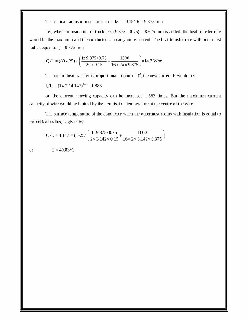
The critical radius of insulation, r c = k/h = 0.15/16 = 9.375 mm
i.e., when an insulation of thickness (9.375 - 0.75) = 8.625 mm is added, the heat transfer rate
would be the maximum and the conductor can carry more current. The heat transfer rate with outermost
radius equal to rc = 9.375 mm
Q /L = (80 - 25) / 1n9.375/ 0.75 10002 0.15 16 2 9.375
=14.7 W/m
The rate of heat transfer is proportional to (current)2, the new current I2 would be:
I2/I1 = (14.7 / 4.147)1/2 = 1.883
or, the current carrying capacity can be increased 1.883 times. But the maximum current
capacity of wire would be limited by the permissible temperature at the centre of the wire.
The surface temperature of the conductor when the outermost radius with insulation is equal to
the critical radius, is given by
Q /L = 4.147 = (T-25/ 1n9.375/ 0.75 10002 3.142 0.15 16 2 3.142 9.375
or T = 40.83°C
UNIT IV
Heat Transfer with Change of Phase
5.2.1. Condensation and Boiling
Heat energy is being converted into electrical energy with the help of water as a working fluid.
Water is first converted into steam when heated in a heat exchanger and then the exhaust steam coming
out of the steam turbine/engine is condensed in a condenser so that the condensate (water) is recycled
again for power generation. Therefore, the condensation and boiling processes involve heat transfer with
change of phase. When a fluid changes its phase, the magnitude of its properties like density, viscosity,
thermal conductivity, specific heat capacity, etc., change appreciably and the processes taking place are
greatly influenced by them. Thus, the condensation and boiling processes must be well understood for
an effective design of different types of heat exchangers being used in thermal and nuclear power plants,
and in process cooling and heating systems.
5.2.2. Condensation-Filmwise and Dropwise
Condensation is the process of transition from a vapour to the liquid or solid state. The process
is accompanied by liberation of heat energy due to the change 10 phase. When a vapour comes 10
contact with a surface maintained at a temperature lower than the saturation temperature of the vapour
corresponding to the pressure at which it exists, the vapour condenses on the surface and the heat energy
thus released has to be removed. The efficiency of the condensing unit is determined by the mode of
condensation that takes place:
Filmwise - the condensing vapour forms a continuous film covering the entire surface,
Dropwise - the vapour condenses into small liquid droplets of various sizes. The dropwise
condensation has a much higher rate of heat transfer than filmwise condensation because the condensate
in dropwise condensation gets removed at a faster rate leading to better heat transfer between the vapour
and the bare surface. .
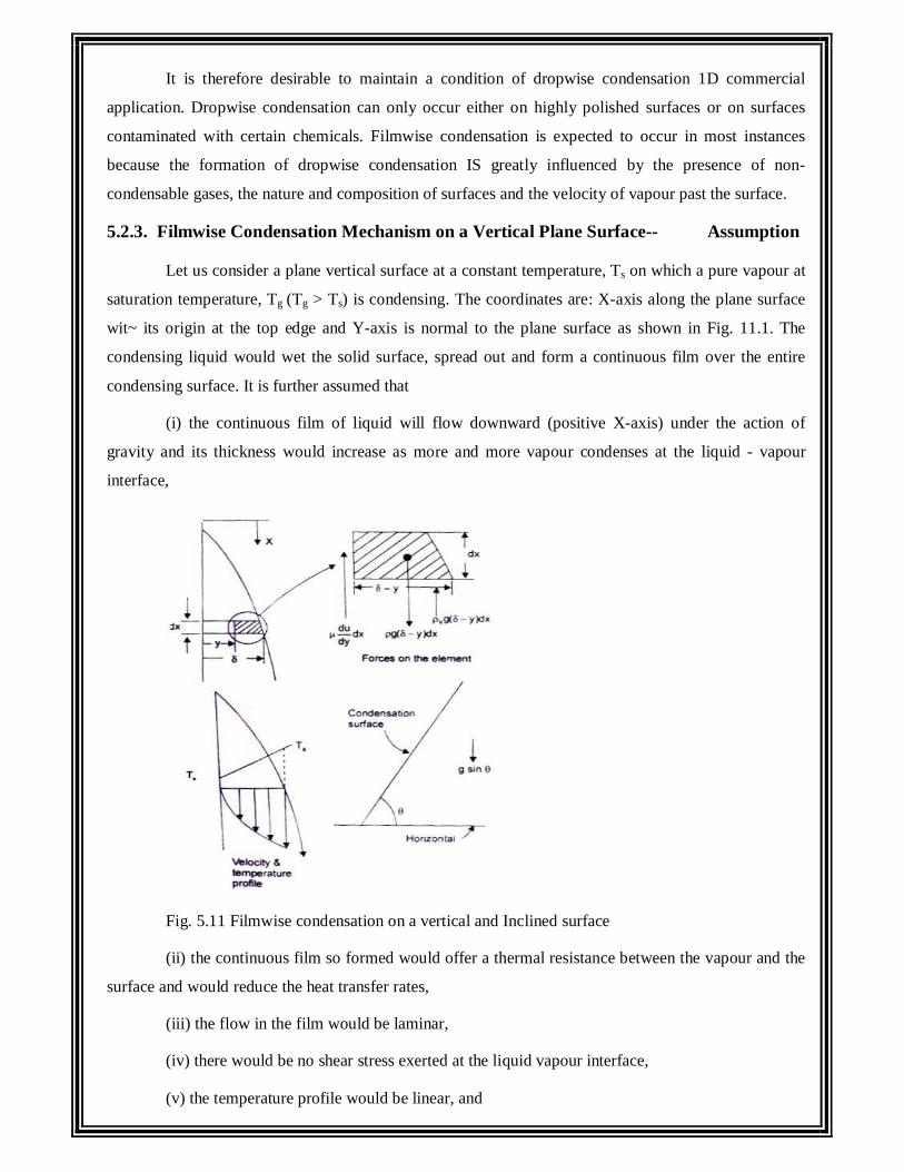
It is therefore desirable to maintain a condition of dropwise condensation 1D commercial
application. Dropwise condensation can only occur either on highly polished surfaces or on surfaces
contaminated with certain chemicals. Filmwise condensation is expected to occur in most instances
because the formation of dropwise condensation IS greatly influenced by the presence of non-
condensable gases, the nature and composition of surfaces and the velocity of vapour past the surface.
5.2.3. Filmwise Condensation Mechanism on a Vertical Plane Surface-- Assumption
Let us consider a plane vertical surface at a constant temperature, Ts on which a pure vapour at
saturation temperature, Tg (Tg > Ts) is condensing. The coordinates are: X-axis along the plane surface
wit~ its origin at the top edge and Y-axis is normal to the plane surface as shown in Fig. 11.1. The
condensing liquid would wet the solid surface, spread out and form a continuous film over the entire
condensing surface. It is further assumed that
(i) the continuous film of liquid will flow downward (positive X-axis) under the action of
gravity and its thickness would increase as more and more vapour condenses at the liquid - vapour
interface,
Fig. 5.11 Filmwise condensation on a vertical and Inclined surface
(ii) the continuous film so formed would offer a thermal resistance between the vapour and the
surface and would reduce the heat transfer rates,
(iii) the flow in the film would be laminar,
(iv) there would be no shear stress exerted at the liquid vapour interface,
(v) the temperature profile would be linear, and
(vi) the weight of the liquid film would be balanced by the viscous shear in the liquid film and
the buoyant force due to the displaced vapour.
5.2.4. An Expression for the Liquid Film Thickness and the Heat Transfer Coefficient in
Laminar Filmwise Condensation on a Vertical Plate
We choose a small element, as shown in Fig. 11.1 and by making a force balance, we write
vg y dx du / dy dx g y dx (5.44)
where is the density of the liquid, v is the density of vapour, is the viscosity of the liquid,
Ii is the thickness of the liquid film at any x, and du/dy is the velocity gradient at x.
Since the no-slip condition requires u = 0 at y = 0, by integration we get:
u = ( - v)g( y - y2/2) / (5.45)
And the mass flow rate of condensate through any x position of the film would be
2v
0 0
m u dy g / y y / 2 dy
3v g / 3 (5.46)
The rate of heat transfer at the wall in the area dx is, for unit width,
g sy 0Q kA dt / dy k dx 1 T T /
,
(temperature distribution is linear)
Since the thickness of the film increases in the positive X-direction, an additional mass of
vapour will condense between x and x + dx, i.e.,
3 3v vg gd d ddx dx
dx 3 d 3 dx
2
v g d
This additional mass of condensing vapour will release heat energy and that has to removed by
conduction through the wall, or,
2v
fg g sg d
h k dx T T /
(5.47)
We can, therefore, determine the thickness, , of the liquid film by integrating Eq. (11.4) with
the boundary condition: at x = 0, = 0,
or,
0.25g s
fg v
4 kx T Tgh
(5.48)
The rate of heat transfer is also related by the relation,
g s g sh dx T T k dx T T / ; or, h k /
which can be expressed In dimensionless form in terms of Nusselt number,
0.253v fg
g s
gh xNu hx / k
4 k T T
(5.49)
The average value of the heat transfer coefficient is obtained by integrating over the length of
the plate:
L
x x0
h 1/ L h dx 4 /3 h L
0.253v fg
Lg s
gh LNu 0.943
k T T
(5.50)
The properties of the liquid in Eq. (5.50) and Eq. (5.49) should be evaluated at the mean
temperature, T = (Tg + Ts)/2.
The above analysis is also applicable to a plane surface inclined at angle with the horizontal,
If g is everywhere replaced by g . sin .
Thus:
Local
0.253v fg
xg s
h x gsinNu 0.707
k T T
and the average
3
v fgL
g s
h L g sinNu 0.943
k T T
(5.51)
These relations should be used with caution for small values of because some of the
assumptions made in deriving these relations become invalid; for example, when is equal to zero, (a
horizontal surface) we would get an absurd result. But these equations are valid for condensation on the
outside surface of vertical tubes as long as the curvature of the tube surface is not too great.
Solution: (a) Tube Homontal: The mean film temperature is (50 + 76) = 63°C, and the
properties are:
3 3980 kg / m , 0.432 10 Pa s, k 0.66 W / mK
fg vh 2320 kJ / kg,
0.252 3
fg g sh 0.725 h k g / D T T
0.252 33 30.725 980 2320 10 0.66 9.81/ 0.432 10 0.015 26
= 10 kW/m2K
(b) Tube Vertical: Eq (5.50) should be used if the film thickness is very small in comparison
with the tube diameter.
The film thickness, 0.25
g s fg v4 kL T T / gh
0.252 33
3980 9.81 2320 10 0.66
0.432 10 1.5 26
= = 0.212 mm << 15.0 mm, the tube diameter.
Therefore, the average heat transfer coefficient would be
0.25 2v hh h / 0.768 L / D 10 / 2.429 4.11 kW / m K
(Thus, the performance of horizontal tubes for filmwise laminar condensation is much better
than vertical tubes and as such horizontal tubes are preferred.)
Example 5.27 A square array of four hundred tubes, 1.5 cm outer diameter is used to condense steam at
atmospheric pressure. The tube walls are maintained at 88°C by a coolant flowing inside
the tubes. Calculate the amount of steam condensed per hour per unit length of the tubes.
Solution: The properties at the mean temperature (88 + 100)/2 = 94°C are:
= 963 kg/mJ, = 3.06 × 10⁻⁴ Pa-s, k = 0.678 W/mK,
hfg = 2255 × 103 J/kg
A square array of 400 tubes will have N = 20. From Eq (5.57),
0.252 3fg g sh 0.725 g k h / N D T T
2 3 329.81 963 0.678 2255 10
0.725 6.328 kW / m K20 0.000306 0.015 12
Surface area for 400 tubes = 400 × 3.142 × 0.015 × 1 (let L = 1)
= 18.852 m2 per metre length of the tube
Q = hA ( T) = 6.328 × 18.852 × 12 = 1431.56 kW
fgm Q / h = 1431.56 × 3600/2255 = 2285.4 kg/hr per metre length.
3 Condensation inside Tubes-Empirical Relation
The condensation of vapours flowing inside a cylindrical tube is of importance in chemical and
petro-chemical industries. The average heat transfer coefficient for vapours condensing inside either
horizontal or vertical tubes can be determined, within 20 percent accuracy, by the relations:
For Reg < 5 × 10⁴, Nud = 5.03 (Reg)1/3 (Pr)1/3
For Reg > 5 × 10⁴, Nud = 0.0265 (Reg)0.8 (Pr)1/3 (5.53)
where Reg is the Reynolds number defined in terms of the mass velocity, or, Reg = DG/ , G
being the mass rate of flow per unit cross-sectional area.
4 Dropwise Condensation-Merits and Demerits
In dropwise condensation, the condensation is found to appear in t he form 0 f individual drops.
These drops increase in size and combine with another drop until their size is great enough that their
weight causes them to run off the surface and the condensing surface is exposed for the formation of a
new drop. This phenomenon has been observed to occur either on highly polished surfaces or on surface
coated/contaminated with certain fatty acids. The heat transfer coefficient in dropwise condensation is
five to ten times higher than the filmwise condensation under similar conditions. It is therefore,
desirable that conditions should be maintained for dropwise condensation in commercial applications.
The presence of non-condensable gases, the nature and composition of the surface, the vapour velocity
past the surface have great influence on the formation of drops on coated/contaminated surfaces and It is
rather difficult to achieve dr0pwlse condensation.
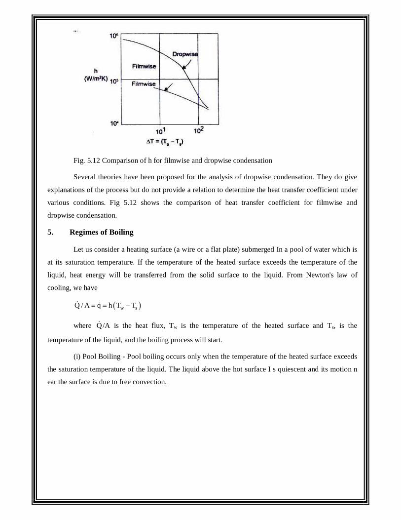
Fig. 5.12 Comparison of h for filmwise and dropwise condensation
Several theories have been proposed for the analysis of dropwise condensation. They do give
explanations of the process but do not provide a relation to determine the heat transfer coefficient under
various conditions. Fig 5.12 shows the comparison of heat transfer coefficient for filmwise and
dropwise condensation.
5. Regimes of Boiling
Let us consider a heating surface (a wire or a flat plate) submerged In a pool of water which is
at its saturation temperature. If the temperature of the heated surface exceeds the temperature of the
liquid, heat energy will be transferred from the solid surface to the liquid. From Newton's law of
cooling, we have
w sQ / A q h T T
where Q /A is the heat flux, Tw is the temperature of the heated surface and Ts, is the
temperature of the liquid, and the boiling process will start.
(i) Pool Boiling - Pool boiling occurs only when the temperature of the heated surface exceeds
the saturation temperature of the liquid. The liquid above the hot surface I s quiescent and its motion n
ear the surface is due to free convection.
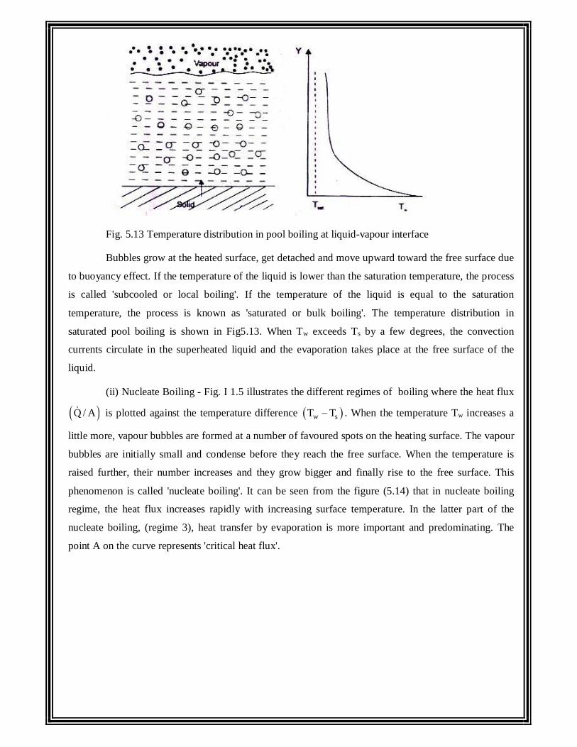
Fig. 5.13 Temperature distribution in pool boiling at liquid-vapour interface
Bubbles grow at the heated surface, get detached and move upward toward the free surface due
to buoyancy effect. If the temperature of the liquid is lower than the saturation temperature, the process
is called 'subcooled or local boiling'. If the temperature of the liquid is equal to the saturation
temperature, the process is known as 'saturated or bulk boiling'. The temperature distribution in
saturated pool boiling is shown in Fig5.13. When Tw exceeds Ts by a few degrees, the convection
currents circulate in the superheated liquid and the evaporation takes place at the free surface of the
liquid.
(ii) Nucleate Boiling - Fig. I 1.5 illustrates the different regimes of boiling where the heat flux
Q / A is plotted against the temperature difference w sT T . When the temperature Tw increases a
little more, vapour bubbles are formed at a number of favoured spots on the heating surface. The vapour
bubbles are initially small and condense before they reach the free surface. When the temperature is
raised further, their number increases and they grow bigger and finally rise to the free surface. This
phenomenon is called 'nucleate boiling'. It can be seen from the figure (5.14) that in nucleate boiling
regime, the heat flux increases rapidly with increasing surface temperature. In the latter part of the
nucleate boiling, (regime 3), heat transfer by evaporation is more important and predominating. The
point A on the curve represents 'critical heat flux'.
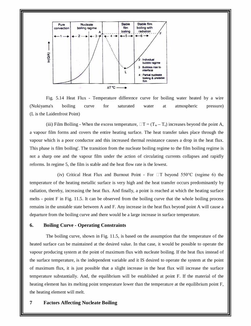
Fig. 5.14 Heat Flux - Temperature difference curve for boiling water heated by a wire
(Nukiyama's boiling curve for saturated water at atmospheric pressure)
(L is the Laidenfrost Point)
(iii) Film Bolling - When the excess temperature, T = (Tw – Ts) increases beyond the point A,
a vapour film forms and covers the entire heating surface. The heat transfer takes place through the
vapour which is a poor conductor and this increased thermal resistance causes a drop in the heat flux.
This phase is film boiling'. The transition from the nucleate boiling regime to the film boiling regime is
not a sharp one and the vapour film under the action of circulating currents collapses and rapidly
reforms. In regime 5, the film is stable and the heat flow rate is the lowest.
(iv) Critical Heat Flux and Burnout Point - For T beyond 550°C (regime 6) the
temperature of the heating metallic surface is very high and the heat transfer occurs predominantly by
radiation, thereby, increasing the heat flux. And finally, a point is reached at which the heating surface
melts - point F in Fig. 11.5. It can be observed from the boiling curve that the whole boiling process
remains in the unstable state between A and F. Any increase in the heat flux beyond point A will cause a
departure from the boiling curve and there would be a large increase in surface temperature.
6. Boiling Curve - Operating Constraints
The boiling curve, shown in Fig. 11.5, is based on the assumption that the temperature of the
heated surface can be maintained at the desired value. In that case, it would be possible to operate the
vapour producing system at the point of maximum flux with nucleate boiling. If the heat flux instead of
the surface temperature, is the independent variable and it IS desired to operate the system at the point
of maximum flux, it is just possible that a slight increase in the heat flux will increase the surface
temperature substantially. And, the equilibrium will be established at point F. If the material of the
heating element has its melting point temperature lower than the temperature at the equilibrium point F,
the heating element will melt.
7 Factors Affecting Nucleate Boiling
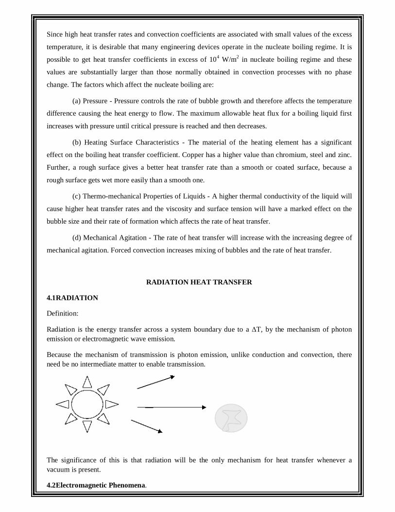
Since high heat transfer rates and convection coefficients are associated with small values of the excess
temperature, it is desirable that many engineering devices operate in the nucleate boiling regime. It is
possible to get heat transfer coefficients in excess of 104 W/m2 in nucleate boiling regime and these
values are substantially larger than those normally obtained in convection processes with no phase
change. The factors which affect the nucleate boiling are:
(a) Pressure - Pressure controls the rate of bubble growth and therefore affects the temperature
difference causing the heat energy to flow. The maximum allowable heat flux for a boiling liquid first
increases with pressure until critical pressure is reached and then decreases.
(b) Heating Surface Characteristics - The material of the heating element has a significant
effect on the boiling heat transfer coefficient. Copper has a higher value than chromium, steel and zinc.
Further, a rough surface gives a better heat transfer rate than a smooth or coated surface, because a
rough surface gets wet more easily than a smooth one.
(c) Thermo-mechanical Properties of Liquids - A higher thermal conductivity of the liquid will
cause higher heat transfer rates and the viscosity and surface tension will have a marked effect on the
bubble size and their rate of formation which affects the rate of heat transfer.
(d) Mechanical Agitation - The rate of heat transfer will increase with the increasing degree of
mechanical agitation. Forced convection increases mixing of bubbles and the rate of heat transfer.
RADIATION HEAT TRANSFER
4.1RADIATION
Definition:
Radiation is the energy transfer across a system boundary due to a ΔT, by the mechanism of photon emission or electromagnetic wave emission.
Because the mechanism of transmission is photon emission, unlike conduction and convection, there need be no intermediate matter to enable transmission.
The significance of this is that radiation will be the only mechanism for heat transfer whenever a vacuum is present.
4.2Electromagnetic Phenomena.
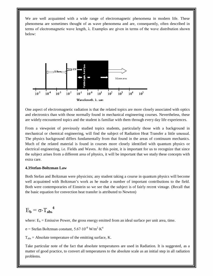
We are well acquainted with a wide range of electromagnetic phenomena in modern life. These phenomena are sometimes thought of as wave phenomena and are, consequently, often described in terms of electromagnetic wave length, λ. Examples are given in terms of the wave distribution shown below:
One aspect of electromagnetic radiation is that the related topics are more closely associated with optics and electronics than with those normally found in mechanical engineering courses. Nevertheless, these are widely encountered topics and the student is familiar with them through every day life experiences.
From a viewpoint of previously studied topics students, particularly those with a background in mechanical or chemical engineering, will find the subject of Radiation Heat Transfer a little unusual. The physics background differs fundamentally from that found in the areas of continuum mechanics. Much of the related material is found in courses more closely identified with quantum physics or electrical engineering, i.e. Fields and Waves. At this point, it is important for us to recognize that since the subject arises from a different area of physics, it will be important that we study these concepts with extra care.
4.3Stefan-Boltzman Law
Both Stefan and Boltzman were physicists; any student taking a course in quantum physics will become well acquainted with Boltzman’s work as he made a number of important contributions to the field. Both were contemporaries of Einstein so we see that the subject is of fairly recent vintage. (Recall that the basic equation for convection heat transfer is attributed to Newton)
where: Eb = Emissive Power, the gross energy emitted from an ideal surface per unit area, time.
σ = Stefan Boltzman constant, 5.67⋅10-8 W/m2⋅K4
Tabs = Absolute temperature of the emitting surface, K.
Take particular note of the fact that absolute temperatures are used in Radiation. It is suggested, as a matter of good practice, to convert all temperatures to the absolute scale as an initial step in all radiation problems.
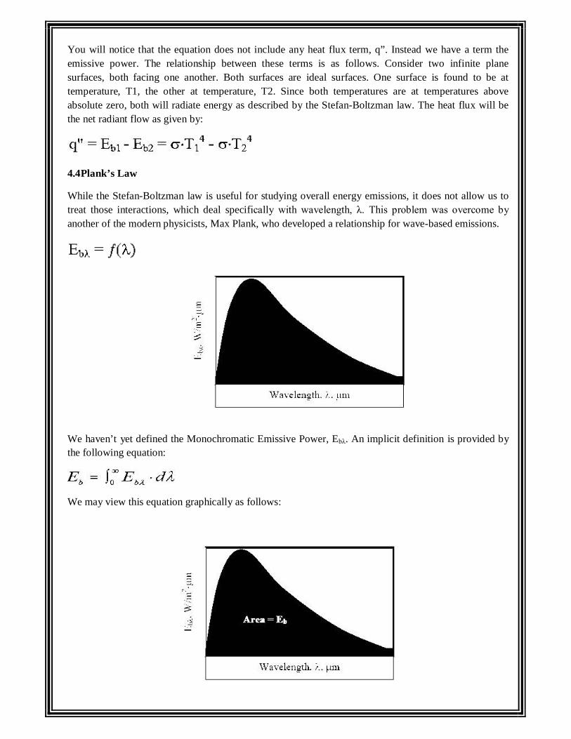
You will notice that the equation does not include any heat flux term, q”. Instead we have a term the emissive power. The relationship between these terms is as follows. Consider two infinite plane surfaces, both facing one another. Both surfaces are ideal surfaces. One surface is found to be at temperature, T1, the other at temperature, T2. Since both temperatures are at temperatures above absolute zero, both will radiate energy as described by the Stefan-Boltzman law. The heat flux will be the net radiant flow as given by:
4.4Plank’s Law
While the Stefan-Boltzman law is useful for studying overall energy emissions, it does not allow us to treat those interactions, which deal specifically with wavelength, λ. This problem was overcome by another of the modern physicists, Max Plank, who developed a relationship for wave-based emissions.
We haven’t yet defined the Monochromatic Emissive Power, Ebλ. An implicit definition is provided by the following equation:
We may view this equation graphically as follows:
A definition of monochromatic Emissive Power would be obtained by differentiating the integral equation:
The actual form of Plank’s law is:
Where: h, co, k are all parameters from quantum physics. We need not worry about their precise definition here.
This equation may be solved at any T, λ to give the value of the monochromatic emissivity at that
condition. Alternatively, the function may be substituted into the integral to find the Emissive power for any temperature. While performing this integral by hand is difficult, students may readily evaluate the integral through one of several computer programs, i.e. MathCad, Maple, Mathmatica, etc.
4.5 Emission Over Specific Wave Length Bands
Consider the problem of designing a tanning machine. As a part of the machine, we will need to design a very powerful incandescent light source. We may wish to know how much energy is being emitted over the
ultraviolet band (10-4 to 0.4 μm), known to be particularly dangerous.
With a computer available, evaluation of this integral is rather trivial. Alternatively, the text books provide a table of integrals. The format used is as follows:
Referring to such tables, we see the last two functions listed in the second column. In the first column is a parameter, λ⋅T. This is found by taking the product of the absolute temperature of the emitting surface, T, and the upper limit wave length, λ. In our example, suppose that the incandescent bulb is designed to operate at a temperature of 2000K. Reading from the table:
λ.,
This is the fraction of the total energy emitted which falls within the IR band. To find the absolute energy emitted multiply this value times the total energy emitted:
4.6 Solar Radiation
The magnitude of the energy leaving the Sun varies with time and is closely associated with such factors as solar flares and sunspots. Nevertheless, we often choose to work with an average value. The energy leaving the sun is emitted outward in all directions so that at any particular distance from the Sun we may imagine the energy being dispersed over an imaginary spherical area. Because this area increases with the distance squared, the solar flux also decreases with the distance squared. At the average distance between Earth and Sun this heat flux is 1353 W/m2, so that the average heat flux on any object in Earth orbit is found as:
Where Sc = Solar Constant, 1353 W/m2
f = correction factor for eccentricity in Earth Orbit, (0.97<f<1.03)
θ = Angle of surface from normal to Sun.
Because of reflection and absorption in the Earth’s atmosphere, this number is significantly reduced at ground level. Nevertheless, this value gives us some opportunity to estimate the potential for using solar energy, such as in photovoltaic cells.
Some Definitions
In the previous section we introduced the Stefan-Boltzman Equation to describe radiation from an ideal surface.
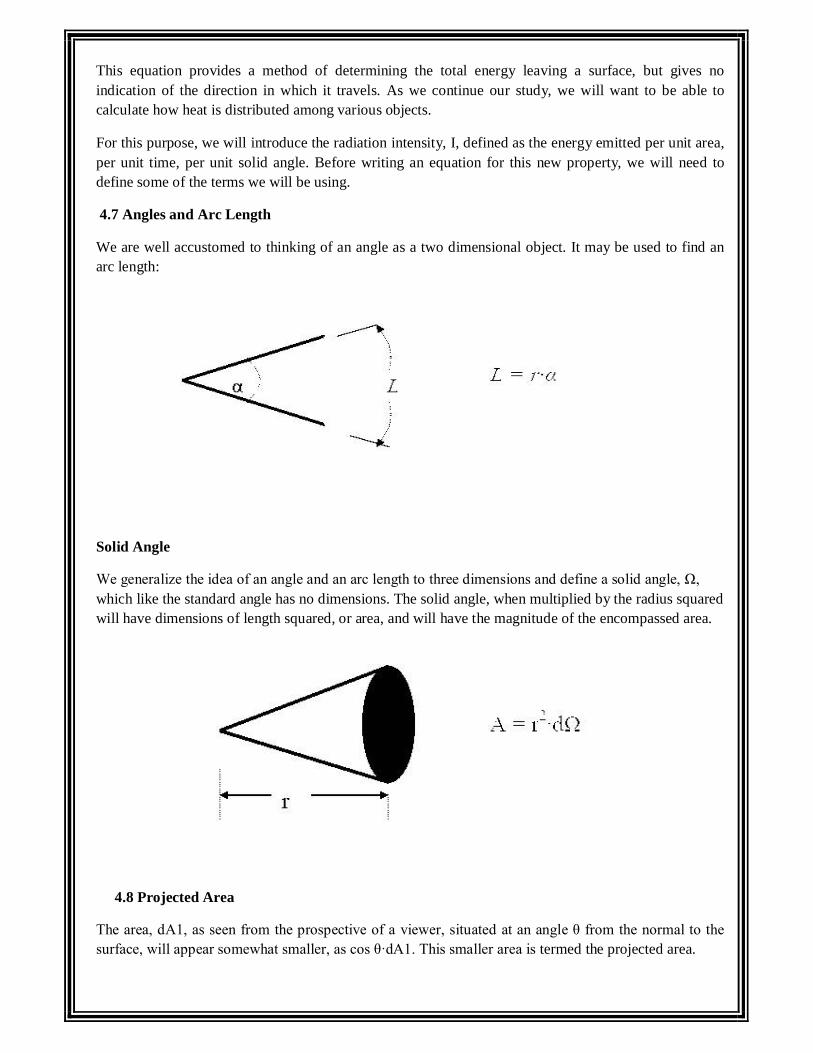
This equation provides a method of determining the total energy leaving a surface, but gives no indication of the direction in which it travels. As we continue our study, we will want to be able to calculate how heat is distributed among various objects.
For this purpose, we will introduce the radiation intensity, I, defined as the energy emitted per unit area, per unit time, per unit solid angle. Before writing an equation for this new property, we will need to define some of the terms we will be using.
4.7 Angles and Arc Length
We are well accustomed to thinking of an angle as a two dimensional object. It may be used to find an arc length:
Solid Angle
We generalize the idea of an angle and an arc length to three dimensions and define a solid angle, Ω, which like the standard angle has no dimensions. The solid angle, when multiplied by the radius squared will have dimensions of length squared, or area, and will have the magnitude of the encompassed area.
4.8 Projected Area
The area, dA1, as seen from the prospective of a viewer, situated at an angle θ from the normal to the surface, will appear somewhat smaller, as cos θ·dA1. This smaller area is termed the projected area.
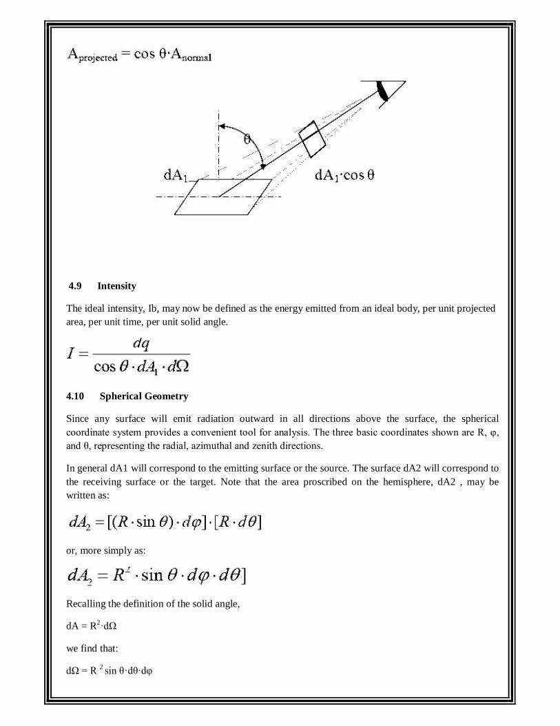
4.9 Intensity
The ideal intensity, Ib, may now be defined as the energy emitted from an ideal body, per unit projected area, per unit time, per unit solid angle.
4.10 Spherical Geometry
Since any surface will emit radiation outward in all directions above the surface, the spherical coordinate system provides a convenient tool for analysis. The three basic coordinates shown are R, φ, and θ, representing the radial, azimuthal and zenith directions.
In general dA1 will correspond to the emitting surface or the source. The surface dA2 will correspond to the receiving surface or the target. Note that the area proscribed on the hemisphere, dA2 , may be written as:
or, more simply as:
Recalling the definition of the solid angle,
dA = R2·dΩ
we find that:
dΩ = R 2 sin θ·dθ·dφ
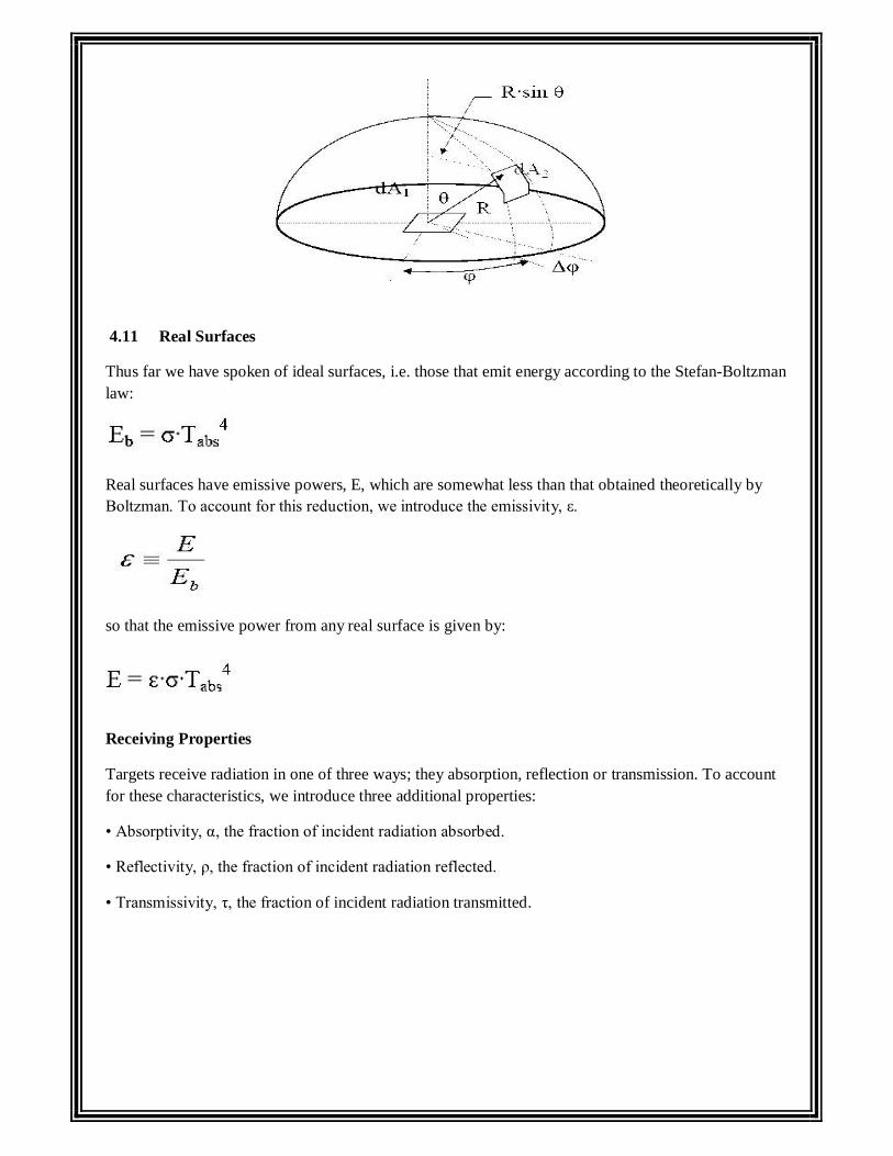
4.11 Real Surfaces
Thus far we have spoken of ideal surfaces, i.e. those that emit energy according to the Stefan-Boltzman law:
Real surfaces have emissive powers, E, which are somewhat less than that obtained theoretically by Boltzman. To account for this reduction, we introduce the emissivity, ε.
so that the emissive power from any real surface is given by:
Receiving Properties
Targets receive radiation in one of three ways; they absorption, reflection or transmission. To account for these characteristics, we introduce three additional properties:
• Absorptivity, α, the fraction of incident radiation absorbed.
• Reflectivity, ρ, the fraction of incident radiation reflected.
• Transmissivity, τ, the fraction of incident radiation transmitted.
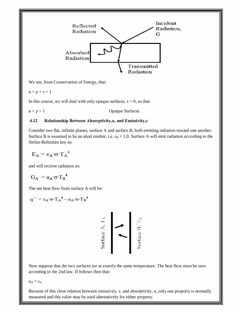
We see, from Conservation of Energy, that:
α + ρ + τ = 1
In this course, we will deal with only opaque surfaces, τ = 0, so that:
α + ρ = 1 Opaque Surfaces
4.12 Relationship Between Absorptivity,α, and Emissivity,ε
Consider two flat, infinite planes, surface A and surface B, both emitting radiation toward one another. Surface B is assumed to be an ideal emitter, i.e. εB = 1.0. Surface A will emit radiation according to the Stefan-Boltzman law as:
and will receive radiation as:
The net heat flow from surface A will be:
Now suppose that the two surfaces are at exactly the same temperature. The heat flow must be zero according to the 2nd law. If follows then that:
αA = εA
Because of this close relation between emissivity, ε, and absorptivity, α, only one property is normally measured and this value may be used alternatively for either property.
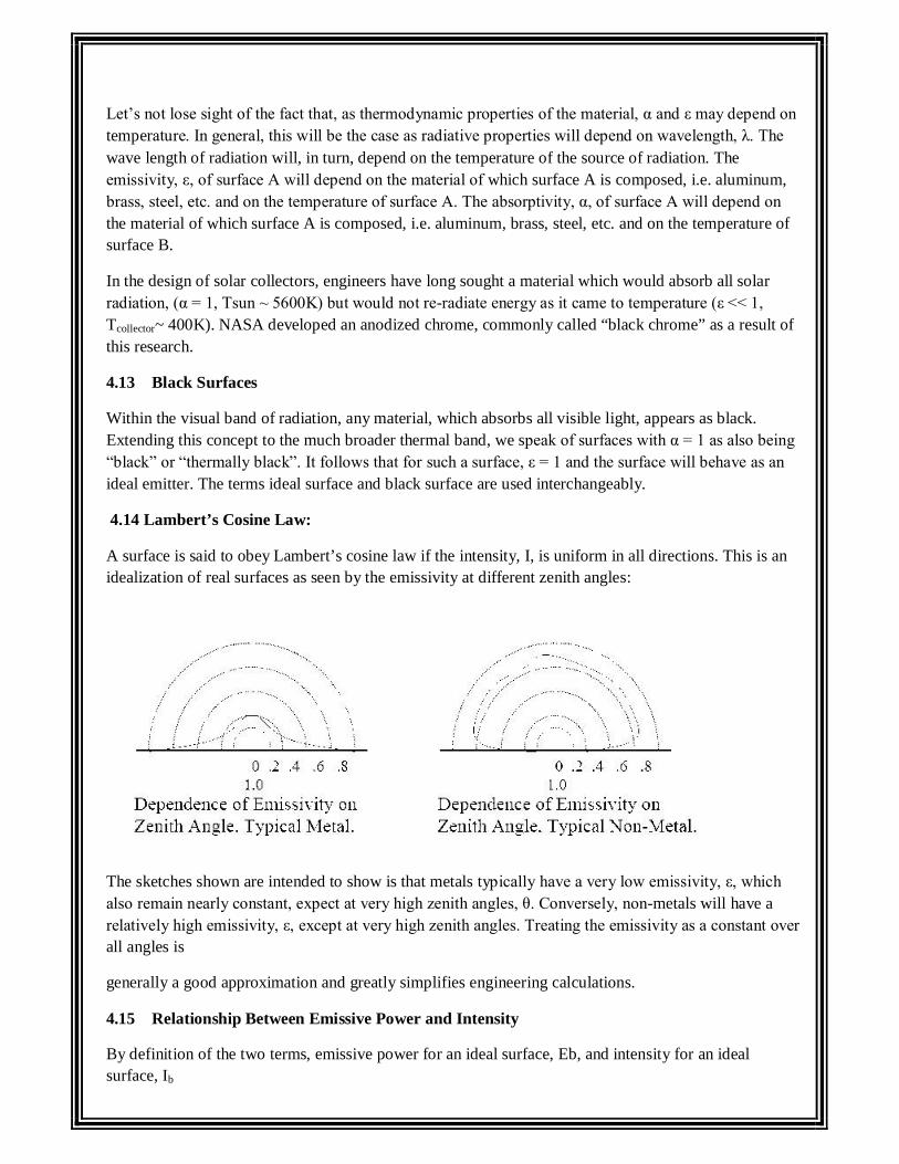
Let’s not lose sight of the fact that, as thermodynamic properties of the material, α and ε may depend on temperature. In general, this will be the case as radiative properties will depend on wavelength, λ. The wave length of radiation will, in turn, depend on the temperature of the source of radiation. The emissivity, ε, of surface A will depend on the material of which surface A is composed, i.e. aluminum, brass, steel, etc. and on the temperature of surface A. The absorptivity, α, of surface A will depend on the material of which surface A is composed, i.e. aluminum, brass, steel, etc. and on the temperature of surface B.
In the design of solar collectors, engineers have long sought a material which would absorb all solar radiation, (α = 1, Tsun ~ 5600K) but would not re-radiate energy as it came to temperature (ε << 1, Tcollector~ 400K). NASA developed an anodized chrome, commonly called “black chrome” as a result of this research.
4.13 Black Surfaces
Within the visual band of radiation, any material, which absorbs all visible light, appears as black. Extending this concept to the much broader thermal band, we speak of surfaces with α = 1 as also being “black” or “thermally black”. It follows that for such a surface, ε = 1 and the surface will behave as an ideal emitter. The terms ideal surface and black surface are used interchangeably.
4.14 Lambert’s Cosine Law:
A surface is said to obey Lambert’s cosine law if the intensity, I, is uniform in all directions. This is an idealization of real surfaces as seen by the emissivity at different zenith angles:
The sketches shown are intended to show is that metals typically have a very low emissivity, ε, which also remain nearly constant, expect at very high zenith angles, θ. Conversely, non-metals will have a relatively high emissivity, ε, except at very high zenith angles. Treating the emissivity as a constant over all angles is
generally a good approximation and greatly simplifies engineering calculations.
4.15 Relationship Between Emissive Power and Intensity
By definition of the two terms, emissive power for an ideal surface, Eb, and intensity for an ideal surface, Ib
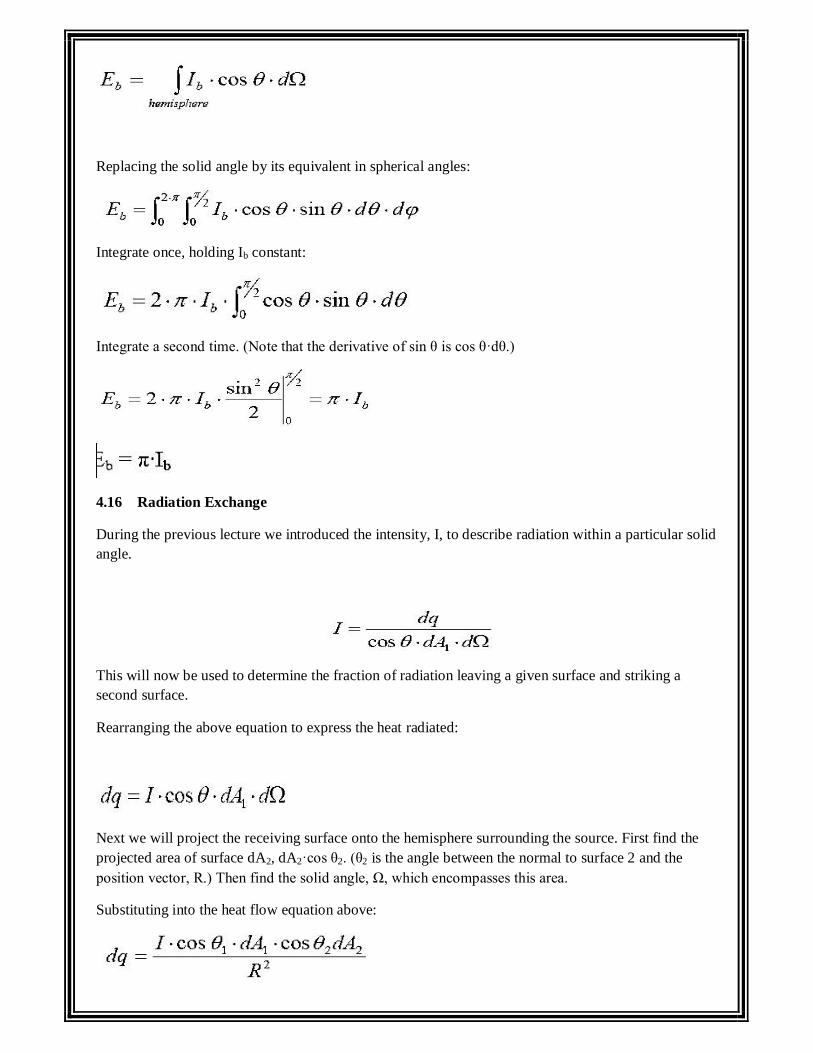
Replacing the solid angle by its equivalent in spherical angles:
Integrate once, holding Ib constant:
Integrate a second time. (Note that the derivative of sin θ is cos θ·dθ.)
4.16 Radiation Exchange
During the previous lecture we introduced the intensity, I, to describe radiation within a particular solid angle.
This will now be used to determine the fraction of radiation leaving a given surface and striking a second surface.
Rearranging the above equation to express the heat radiated:
Next we will project the receiving surface onto the hemisphere surrounding the source. First find the projected area of surface dA2, dA2·cos θ2. (θ2 is the angle between the normal to surface 2 and the position vector, R.) Then find the solid angle, Ω, which encompasses this area.
Substituting into the heat flow equation above:
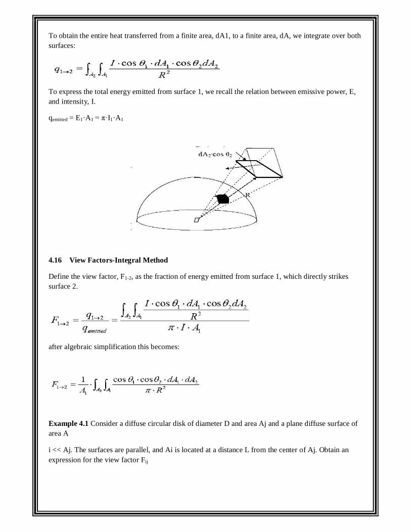
To obtain the entire heat transferred from a finite area, dA1, to a finite area, dA, we integrate over both surfaces:
To express the total energy emitted from surface 1, we recall the relation between emissive power, E, and intensity, I.
qemitted = E1·A1 = π·I1·A1
4.16 View Factors-Integral Method
Define the view factor, F1-2, as the fraction of energy emitted from surface 1, which directly strikes surface 2.
after algebraic simplification this becomes:
Example 4.1 Consider a diffuse circular disk of diameter D and area Aj and a plane diffuse surface of area A
i << Aj. The surfaces are parallel, and Ai is located at a distance L from the center of Aj. Obtain an expression for the view factor Fij
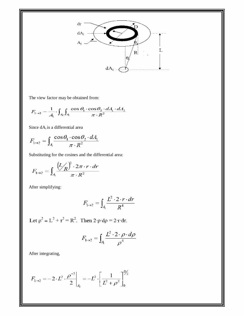
The view factor may be obtained from:
Since dAi is a differential area
Substituting for the cosines and the differential area:
After simplifying:
After integrating,
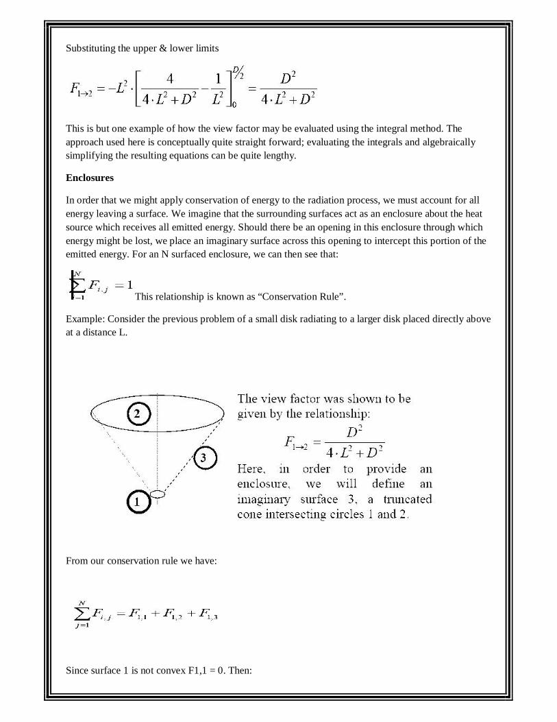
Substituting the upper & lower limits
This is but one example of how the view factor may be evaluated using the integral method. The approach used here is conceptually quite straight forward; evaluating the integrals and algebraically simplifying the resulting equations can be quite lengthy.
Enclosures
In order that we might apply conservation of energy to the radiation process, we must account for all energy leaving a surface. We imagine that the surrounding surfaces act as an enclosure about the heat source which receives all emitted energy. Should there be an opening in this enclosure through which energy might be lost, we place an imaginary surface across this opening to intercept this portion of the emitted energy. For an N surfaced enclosure, we can then see that:
This relationship is known as “Conservation Rule”.
Example: Consider the previous problem of a small disk radiating to a larger disk placed directly above at a distance L.
From our conservation rule we have:
Since surface 1 is not convex F1,1 = 0. Then:
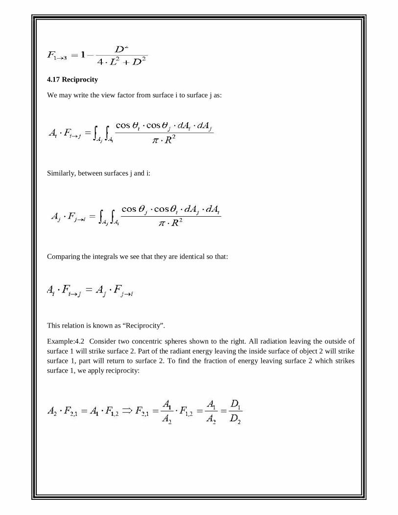
4.17 Reciprocity
We may write the view factor from surface i to surface j as:
Similarly, between surfaces j and i:
Comparing the integrals we see that they are identical so that:
This relation is known as “Reciprocity”.
Example:4.2 Consider two concentric spheres shown to the right. All radiation leaving the outside of surface 1 will strike surface 2. Part of the radiant energy leaving the inside surface of object 2 will strike surface 1, part will return to surface 2. To find the fraction of energy leaving surface 2 which strikes surface 1, we apply reciprocity:
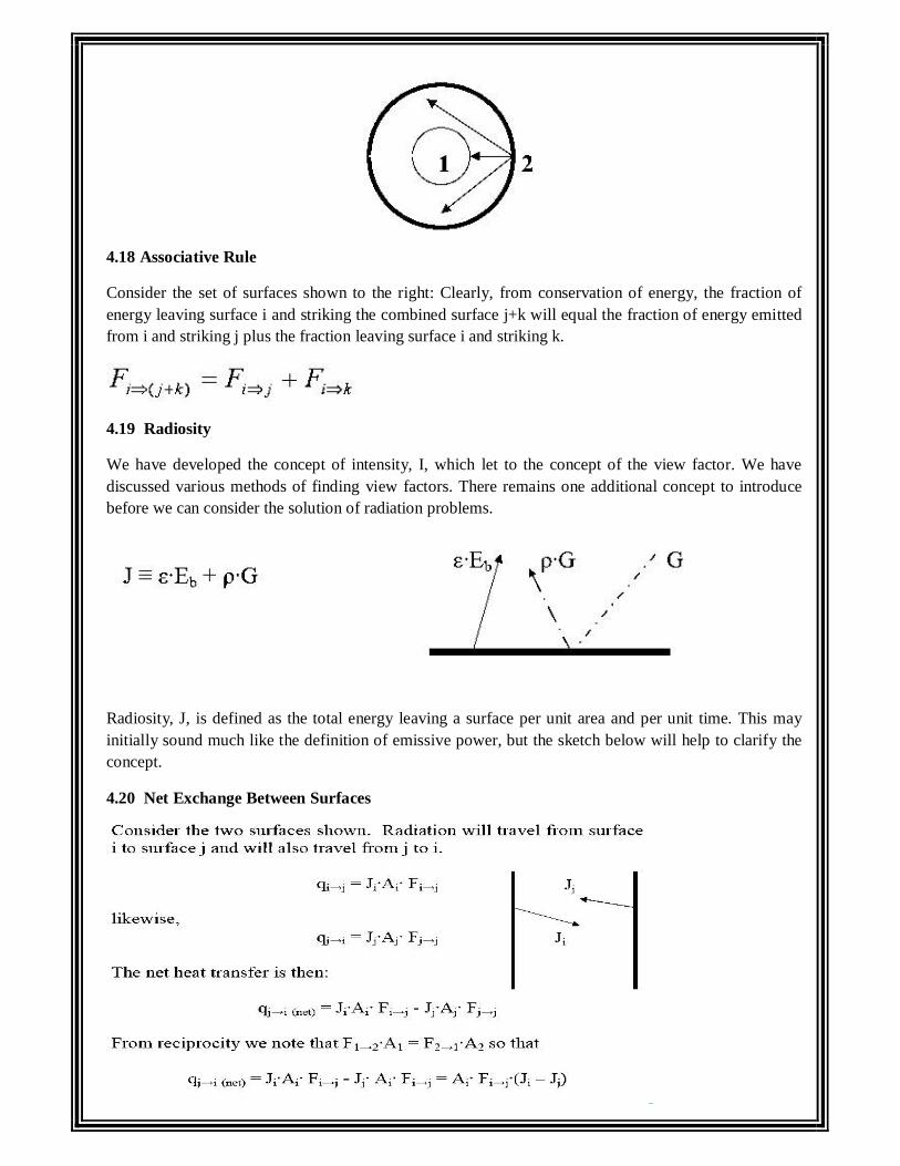
4.18 Associative Rule
Consider the set of surfaces shown to the right: Clearly, from conservation of energy, the fraction of energy leaving surface i and striking the combined surface j+k will equal the fraction of energy emitted from i and striking j plus the fraction leaving surface i and striking k.
4.19 Radiosity
We have developed the concept of intensity, I, which let to the concept of the view factor. We have discussed various methods of finding view factors. There remains one additional concept to introduce before we can consider the solution of radiation problems.
Radiosity, J, is defined as the total energy leaving a surface per unit area and per unit time. This may initially sound much like the definition of emissive power, but the sketch below will help to clarify the concept.
4.20 Net Exchange Between Surfaces
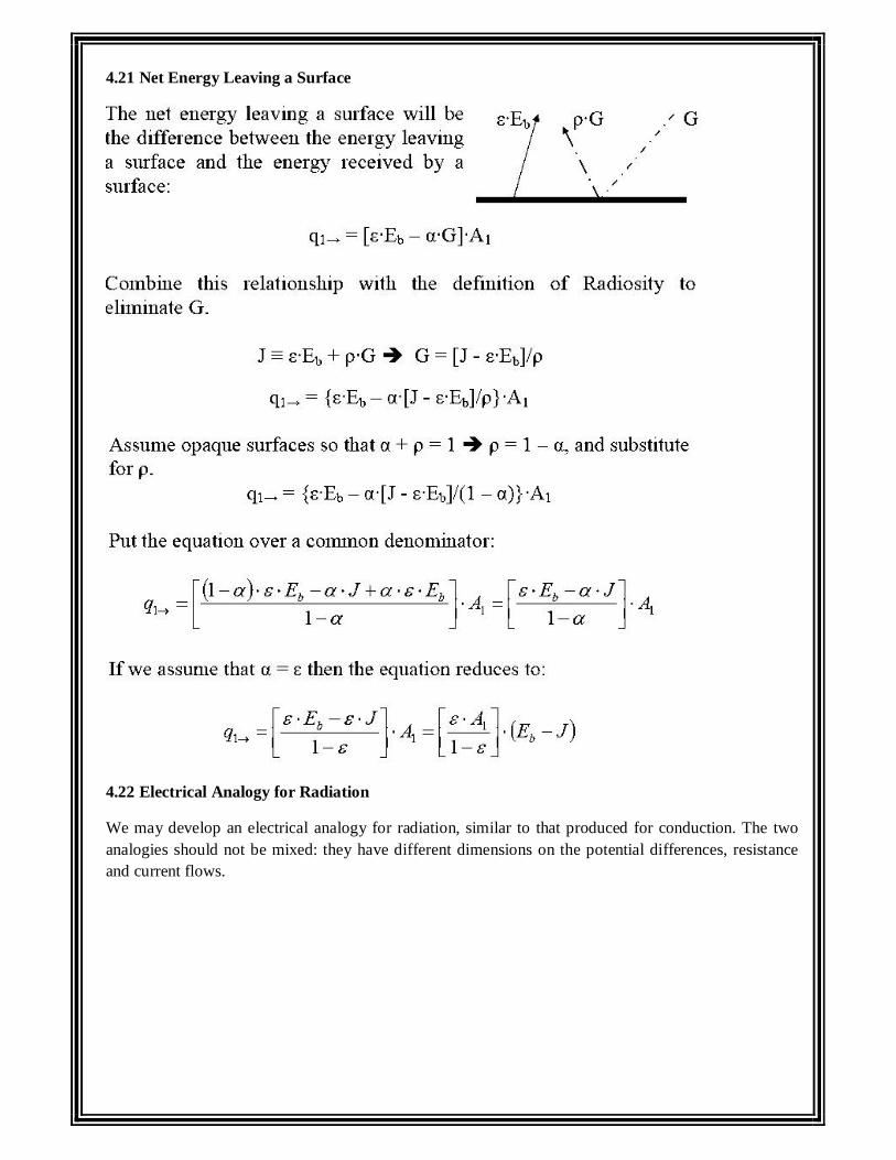
4.21 Net Energy Leaving a Surface
4.22 Electrical Analogy for Radiation
We may develop an electrical analogy for radiation, similar to that produced for conduction. The two analogies should not be mixed: they have different dimensions on the potential differences, resistance and current flows.
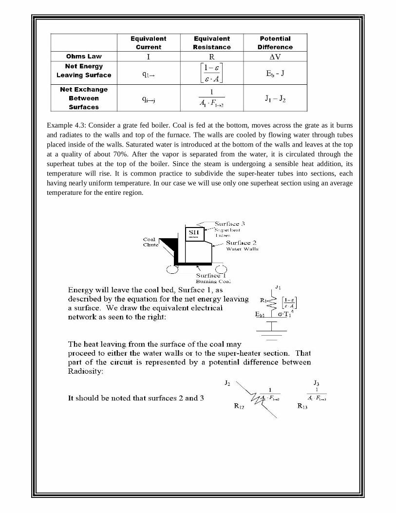
Example 4.3: Consider a grate fed boiler. Coal is fed at the bottom, moves across the grate as it burns and radiates to the walls and top of the furnace. The walls are cooled by flowing water through tubes placed inside of the walls. Saturated water is introduced at the bottom of the walls and leaves at the top at a quality of about 70%. After the vapor is separated from the water, it is circulated through the superheat tubes at the top of the boiler. Since the steam is undergoing a sensible heat addition, its temperature will rise. It is common practice to subdivide the super-heater tubes into sections, each having nearly uniform temperature. In our case we will use only one superheat section using an average temperature for the entire region.
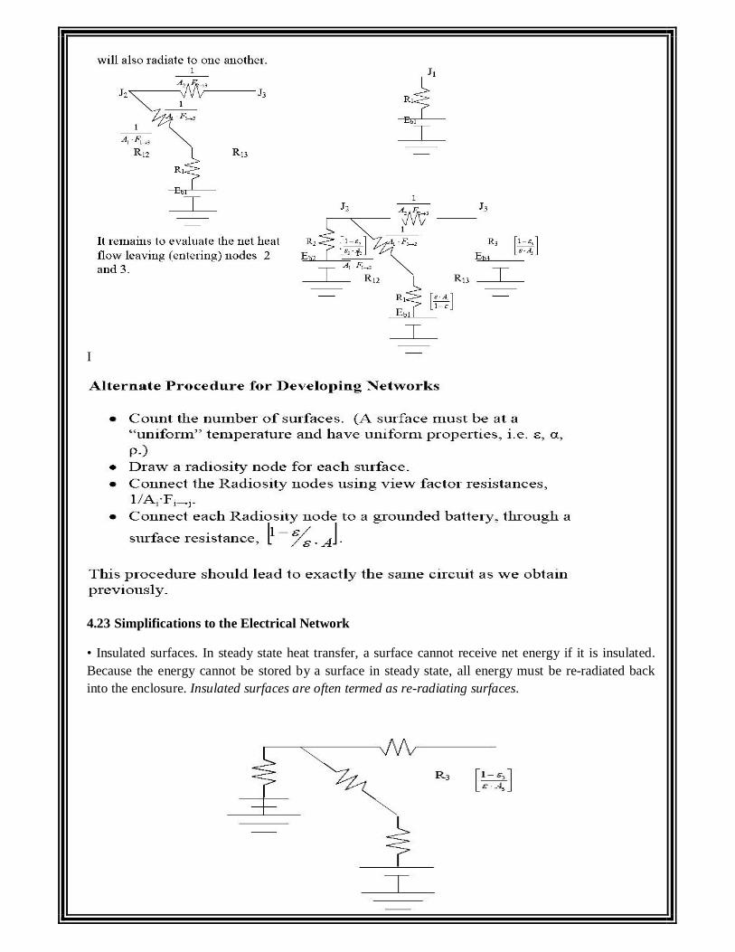
I
4.23 Simplifications to the Electrical Network
• Insulated surfaces. In steady state heat transfer, a surface cannot receive net energy if it is insulated. Because the energy cannot be stored by a surface in steady state, all energy must be re-radiated back into the enclosure. Insulated surfaces are often termed as re-radiating surfaces.
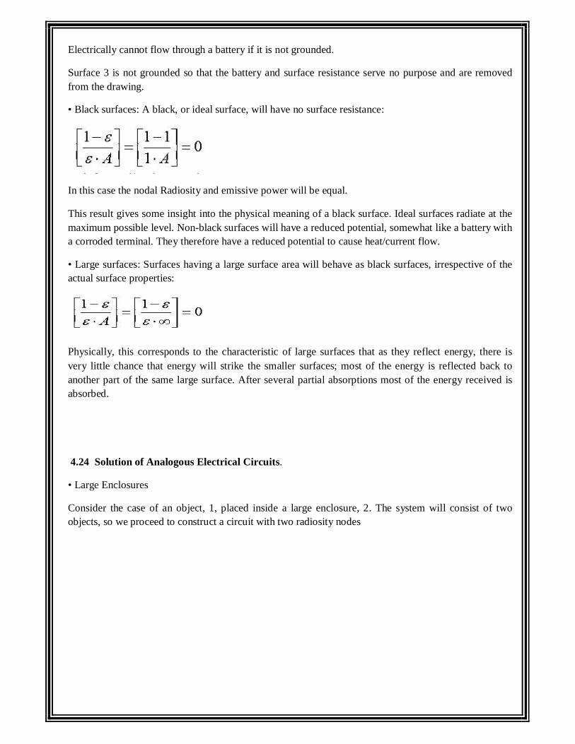
Electrically cannot flow through a battery if it is not grounded.
Surface 3 is not grounded so that the battery and surface resistance serve no purpose and are removed from the drawing.
• Black surfaces: A black, or ideal surface, will have no surface resistance:
In this case the nodal Radiosity and emissive power will be equal.
This result gives some insight into the physical meaning of a black surface. Ideal surfaces radiate at the maximum possible level. Non-black surfaces will have a reduced potential, somewhat like a battery with a corroded terminal. They therefore have a reduced potential to cause heat/current flow.
• Large surfaces: Surfaces having a large surface area will behave as black surfaces, irrespective of the actual surface properties:
Physically, this corresponds to the characteristic of large surfaces that as they reflect energy, there is very little chance that energy will strike the smaller surfaces; most of the energy is reflected back to another part of the same large surface. After several partial absorptions most of the energy received is absorbed.
4.24 Solution of Analogous Electrical Circuits.
• Large Enclosures
Consider the case of an object, 1, placed inside a large enclosure, 2. The system will consist of two objects, so we proceed to construct a circuit with two radiosity nodes
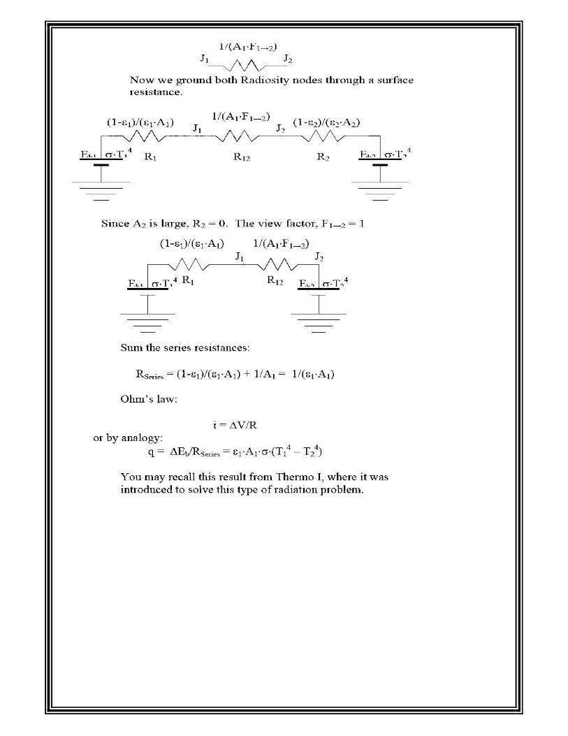
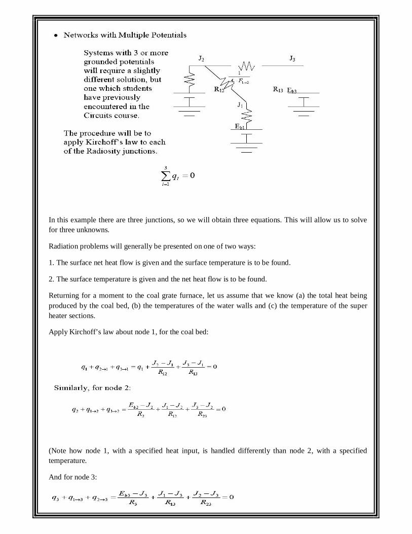
In this example there are three junctions, so we will obtain three equations. This will allow us to solve for three unknowns.
Radiation problems will generally be presented on one of two ways:
1. The surface net heat flow is given and the surface temperature is to be found.
2. The surface temperature is given and the net heat flow is to be found.
Returning for a moment to the coal grate furnace, let us assume that we know (a) the total heat being produced by the coal bed, (b) the temperatures of the water walls and (c) the temperature of the super heater sections.
Apply Kirchoff’s law about node 1, for the coal bed:
(Note how node 1, with a specified heat input, is handled differently than node 2, with a specified temperature.
And for node 3:
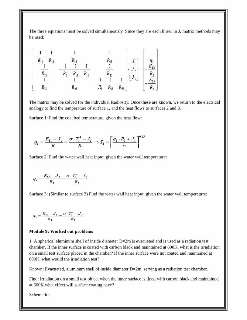
The three equations must be solved simultaneously. Since they are each linear in J, matrix methods may be used:
The matrix may be solved for the individual Radiosity. Once these are known, we return to the electrical analogy to find the temperature of surface 1, and the heat flows to surfaces 2 and 3.
Surface 1: Find the coal bed temperature, given the heat flow:
Surface 2: Find the water wall heat input, given the water wall temperature:
Surface 3: (Similar to surface 2) Find the water wall heat input, given the water wall temperature:
Module 9: Worked out problems
1. A spherical aluminum shell of inside diameter D=2m is evacuated and is used as a radiation test chamber. If the inner surface is coated with carbon black and maintained at 600K, what is the irradiation on a small test surface placed in the chamber? If the inner surface were not coated and maintained at 600K, what would the irradiation test?
Known: Evacuated, aluminum shell of inside diameter D=2m, serving as a radiation test chamber.
Find: Irradiation on a small test object when the inner surface is lined with carbon black and maintained at 600K.what effect will surface coating have?
Schematic:
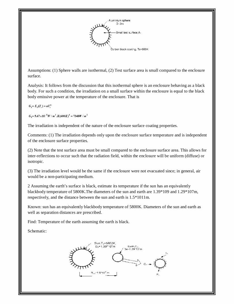
Assumptions: (1) Sphere walls are isothermal, (2) Test surface area is small compared to the enclosure surface.
Analysis: It follows from the discussion that this isothermal sphere is an enclosure behaving as a black body. For such a condition, the irradiation on a small surface within the enclosure is equal to the black body emissive power at the temperature of the enclosure. That is
The irradiation is independent of the nature of the enclosure surface coating properties.
Comments: (1) The irradiation depends only upon the enclosure surface temperature and is independent of the enclosure surface properties.
(2) Note that the test surface area must be small compared to the enclosure surface area. This allows for inter-reflections to occur such that the radiation field, within the enclosure will be uniform (diffuse) or isotropic.
(3) The irradiation level would be the same if the enclosure were not evacuated since; in general, air would be a non-participating medium.
2 Assuming the earth’s surface is black, estimate its temperature if the sun has an equivalently blackbody temperature of 5800K.The diameters of the sun and earth are 1.39*109 and 1.29*107m, respectively, and the distance between the sun and earth is 1.5*1011m.
Known: sun has an equivalently blackbody temperature of 5800K. Diameters of the sun and earth as well as separation distances are prescribed.
Find: Temperature of the earth assuming the earth is black.
Schematic:
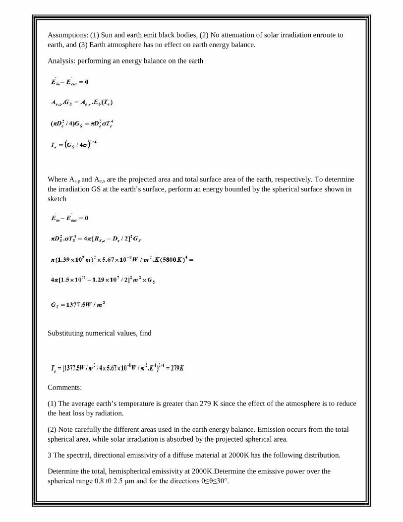
Assumptions: (1) Sun and earth emit black bodies, (2) No attenuation of solar irradiation enroute to earth, and (3) Earth atmosphere has no effect on earth energy balance.
Analysis: performing an energy balance on the earth
Where As,p and Ae,s are the projected area and total surface area of the earth, respectively. To determine the irradiation GS at the earth’s surface, perform an energy bounded by the spherical surface shown in sketch
Substituting numerical values, find
Comments:
(1) The average earth’s temperature is greater than 279 K since the effect of the atmosphere is to reduce the heat loss by radiation.
(2) Note carefully the different areas used in the earth energy balance. Emission occurs from the total spherical area, while solar irradiation is absorbed by the projected spherical area.
3 The spectral, directional emissivity of a diffuse material at 2000K has the following distribution.
Determine the total, hemispherical emissivity at 2000K.Determine the emissive power over the spherical range 0.8 t0 2.5 μm and for the directions 0≤θ≤30°.
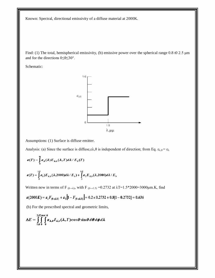
Known: Spectral, directional emissivity of a diffuse material at 2000K.
Find: (1) The total, hemispherical emissivity, (b) emissive power over the spherical range 0.8 t0 2.5 μm and for the directions 0≤θ≤30°.
Schematic:
Assumptions: (1) Surface is diffuse emitter.
Analysis: (a) Since the surface is diffuse,ελ,θ is independent of direction; from Eq. ελ,θ = ελ
Written now in terms of F (0→λ), with F (0→1.5) =0.2732 at λT=1.5*2000=3000μm.K, find
(b) For the prescribed spectral and geometric limits,
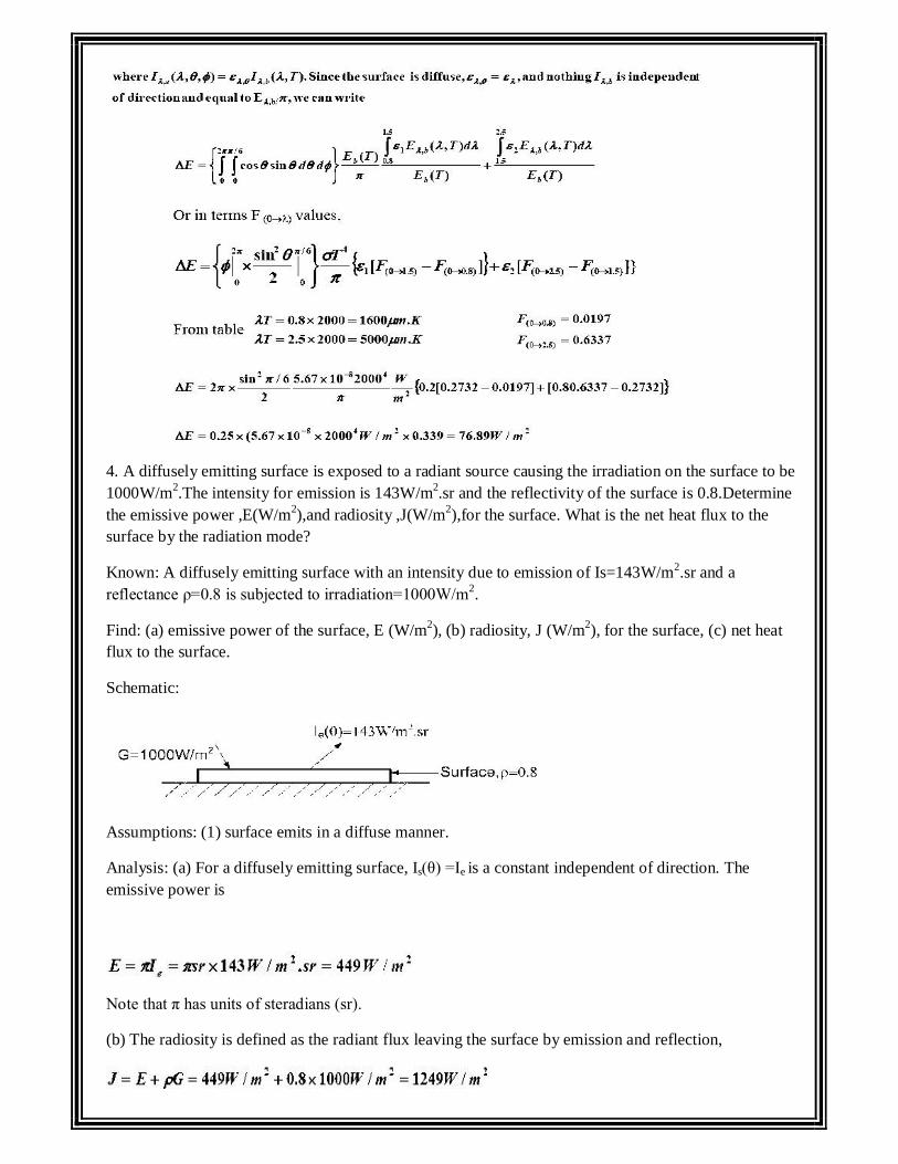
4. A diffusely emitting surface is exposed to a radiant source causing the irradiation on the surface to be 1000W/m2.The intensity for emission is 143W/m2.sr and the reflectivity of the surface is 0.8.Determine the emissive power ,E(W/m2),and radiosity ,J(W/m2),for the surface. What is the net heat flux to the surface by the radiation mode?
Known: A diffusely emitting surface with an intensity due to emission of Is=143W/m2.sr and a reflectance ρ=0.8 is subjected to irradiation=1000W/m2.
Find: (a) emissive power of the surface, E (W/m2), (b) radiosity, J (W/m2), for the surface, (c) net heat flux to the surface.
Schematic:
Assumptions: (1) surface emits in a diffuse manner.
Analysis: (a) For a diffusely emitting surface, Is(θ) =Ie is a constant independent of direction. The emissive power is
Note that π has units of steradians (sr).
(b) The radiosity is defined as the radiant flux leaving the surface by emission and reflection,
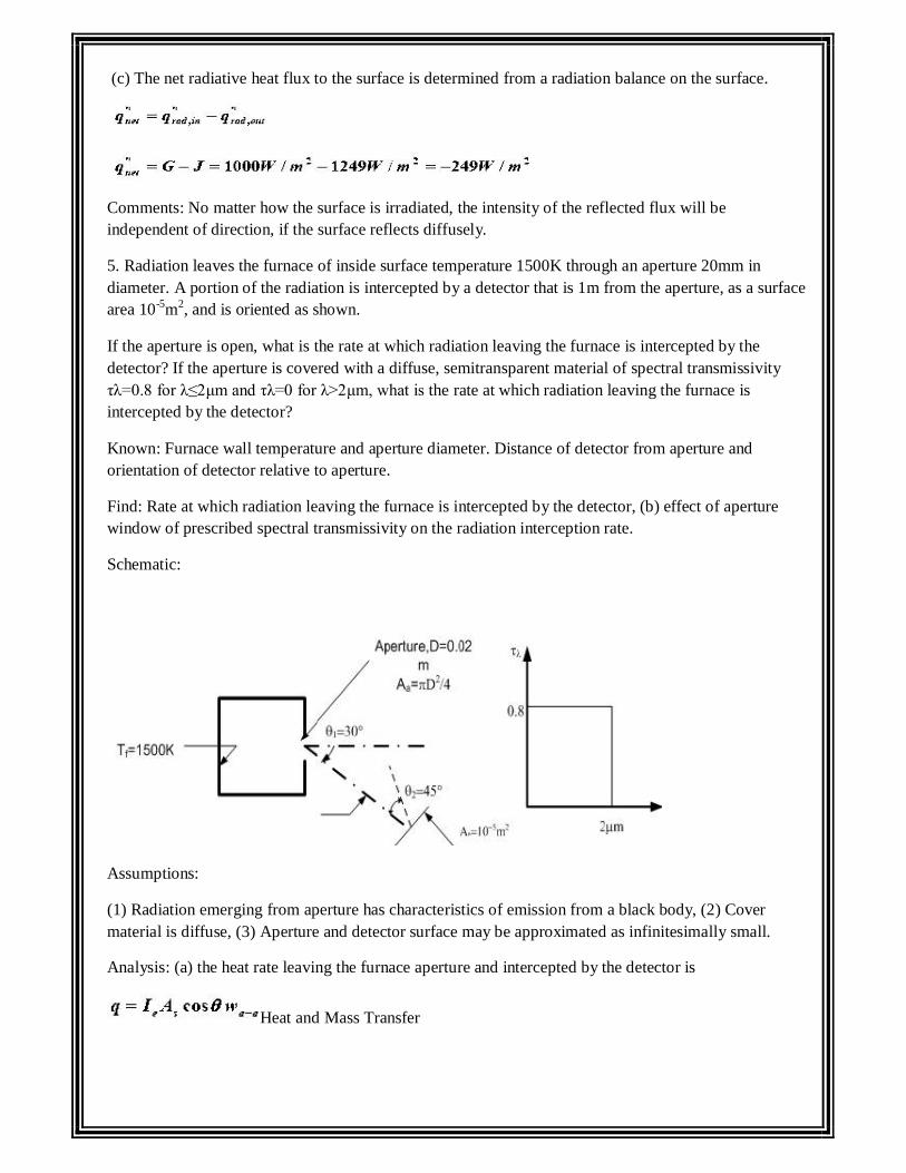
(c) The net radiative heat flux to the surface is determined from a radiation balance on the surface.
Comments: No matter how the surface is irradiated, the intensity of the reflected flux will be independent of direction, if the surface reflects diffusely.
5. Radiation leaves the furnace of inside surface temperature 1500K through an aperture 20mm in diameter. A portion of the radiation is intercepted by a detector that is 1m from the aperture, as a surface area 10-5m2, and is oriented as shown.
If the aperture is open, what is the rate at which radiation leaving the furnace is intercepted by the detector? If the aperture is covered with a diffuse, semitransparent material of spectral transmissivity τλ=0.8 for λ≤2μm and τλ=0 for λ>2μm, what is the rate at which radiation leaving the furnace is intercepted by the detector?
Known: Furnace wall temperature and aperture diameter. Distance of detector from aperture and orientation of detector relative to aperture.
Find: Rate at which radiation leaving the furnace is intercepted by the detector, (b) effect of aperture window of prescribed spectral transmissivity on the radiation interception rate.
Schematic:
Assumptions:
(1) Radiation emerging from aperture has characteristics of emission from a black body, (2) Cover material is diffuse, (3) Aperture and detector surface may be approximated as infinitesimally small.
Analysis: (a) the heat rate leaving the furnace aperture and intercepted by the detector is
Heat and Mass Transfer
Hence
(b) With the window, the heat rate is
6.A horizontal semitransparent plate is uniformly irradiated from above and below, while air at T=300K flows over the top and bottom surfaces. providing a uniform convection heat transfer coefficient of h=40W/m2.K.the total, hemispherical absorptivity of the plate to the irradiation is 0.40.Under steady-state conditions measurements made with radiation detector above the top surface indicate a radiosity(which includes transmission, as well as reflection and emission) of J=5000W/m2,while the plate is at uniform temperature of T=350K
Determine the irradiation G and the total hemispherical emissivity of the plate. Is the plate gray for the prescribed conditions?
Known: Temperature, absorptivity, transmissivity, radiosity and convection conditions for a semi-transparent plate.
Find: Plate irradiation and total hemispherical emissivity.
Schematic:
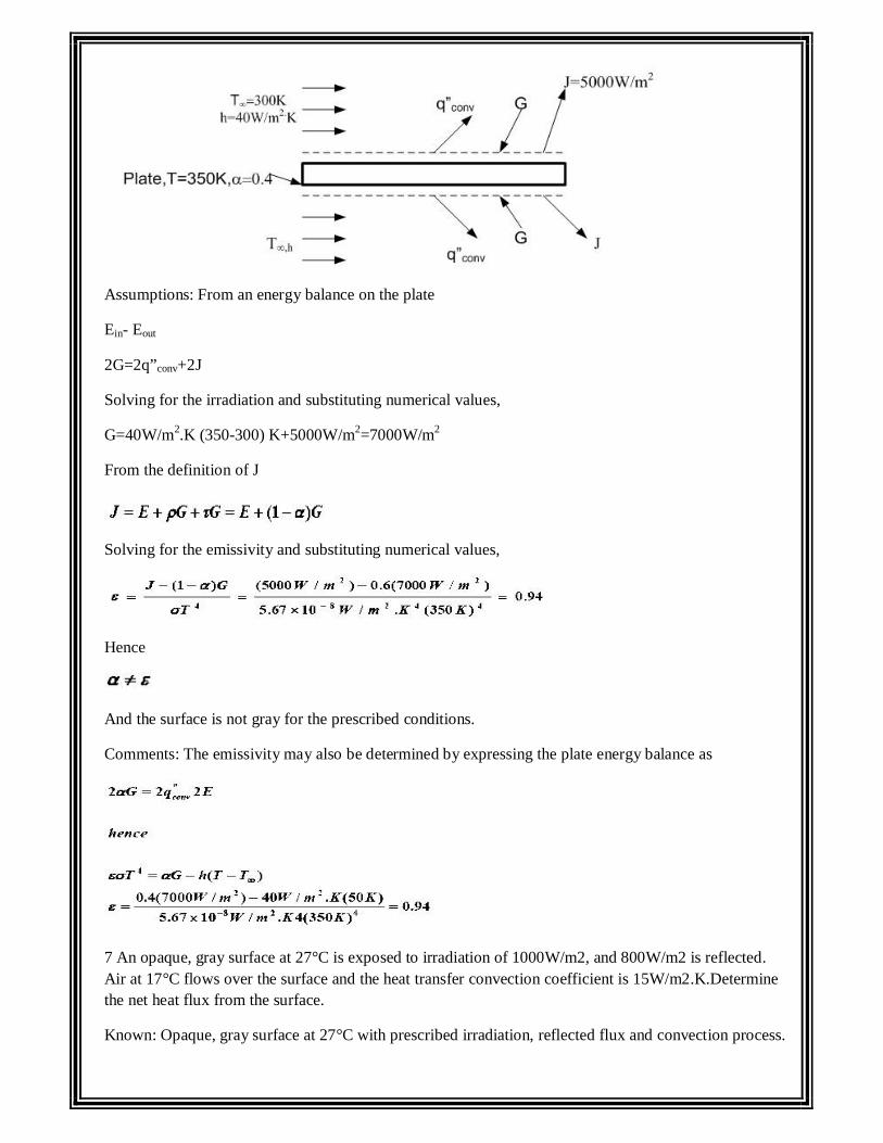
Assumptions: From an energy balance on the plate
Ein- Eout
2G=2q”conv+2J
Solving for the irradiation and substituting numerical values,
G=40W/m2.K (350-300) K+5000W/m2=7000W/m2
From the definition of J
Solving for the emissivity and substituting numerical values,
Hence
And the surface is not gray for the prescribed conditions.
Comments: The emissivity may also be determined by expressing the plate energy balance as
7 An opaque, gray surface at 27°C is exposed to irradiation of 1000W/m2, and 800W/m2 is reflected. Air at 17°C flows over the surface and the heat transfer convection coefficient is 15W/m2.K.Determine the net heat flux from the surface.
Known: Opaque, gray surface at 27°C with prescribed irradiation, reflected flux and convection process.
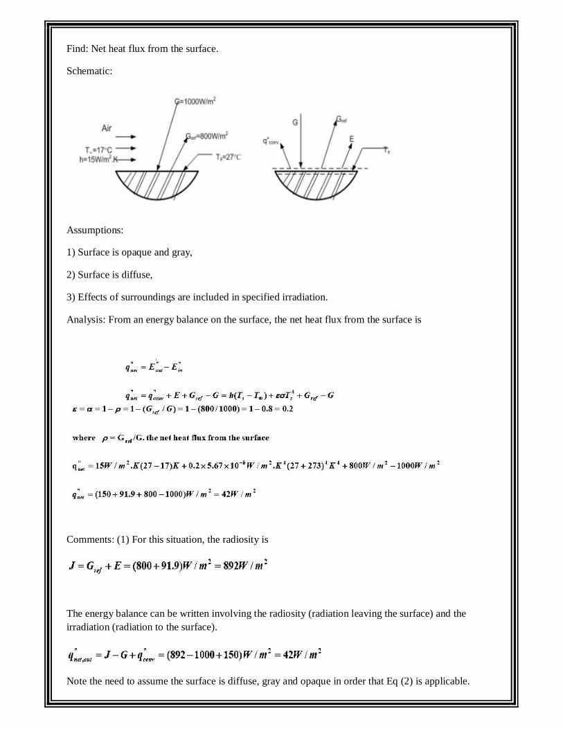
Find: Net heat flux from the surface.
Schematic:
Assumptions:
1) Surface is opaque and gray,
2) Surface is diffuse,
3) Effects of surroundings are included in specified irradiation.
Analysis: From an energy balance on the surface, the net heat flux from the surface is
Comments: (1) For this situation, the radiosity is
The energy balance can be written involving the radiosity (radiation leaving the surface) and the irradiation (radiation to the surface).
Note the need to assume the surface is diffuse, gray and opaque in order that Eq (2) is applicable.
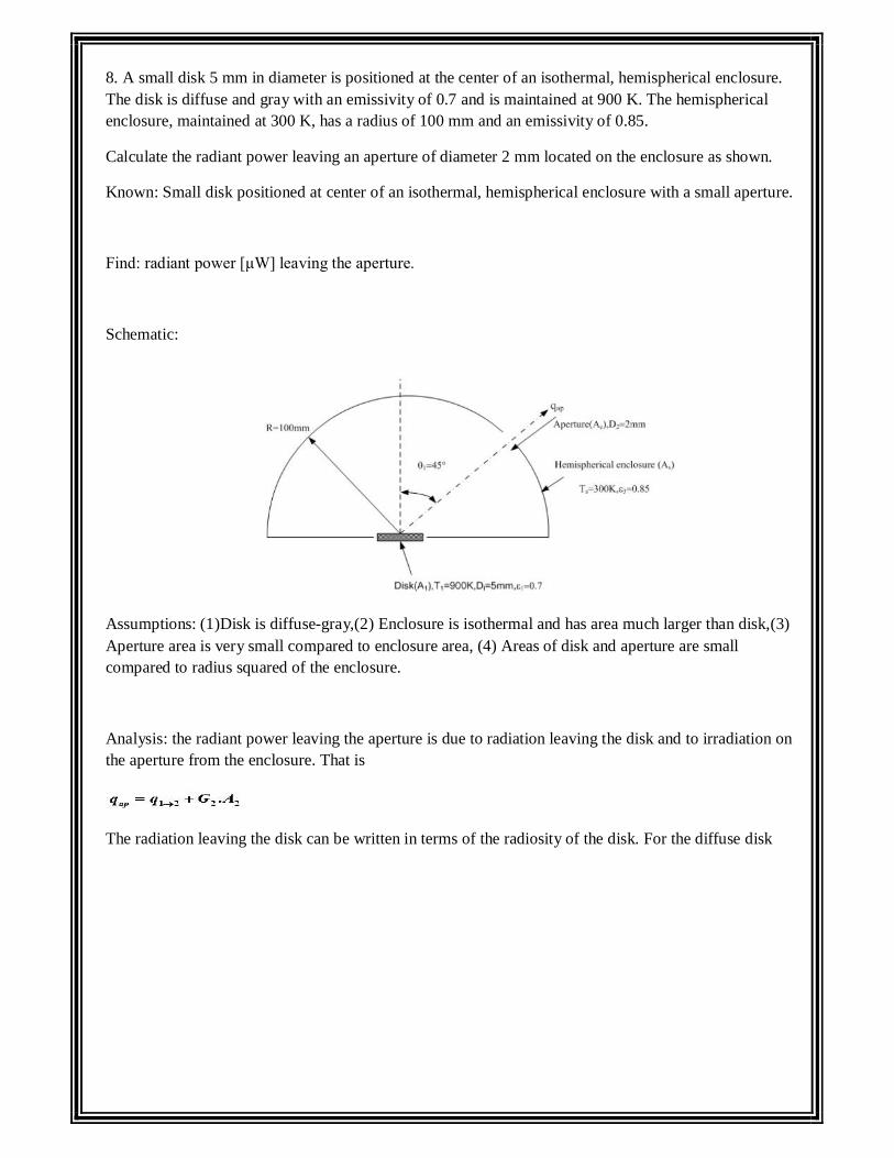
8. A small disk 5 mm in diameter is positioned at the center of an isothermal, hemispherical enclosure. The disk is diffuse and gray with an emissivity of 0.7 and is maintained at 900 K. The hemispherical enclosure, maintained at 300 K, has a radius of 100 mm and an emissivity of 0.85.
Calculate the radiant power leaving an aperture of diameter 2 mm located on the enclosure as shown.
Known: Small disk positioned at center of an isothermal, hemispherical enclosure with a small aperture.
Find: radiant power [μW] leaving the aperture.
Schematic:
Assumptions: (1)Disk is diffuse-gray,(2) Enclosure is isothermal and has area much larger than disk,(3) Aperture area is very small compared to enclosure area, (4) Areas of disk and aperture are small compared to radius squared of the enclosure.
Analysis: the radiant power leaving the aperture is due to radiation leaving the disk and to irradiation on the aperture from the enclosure. That is
The radiation leaving the disk can be written in terms of the radiosity of the disk. For the diffuse disk
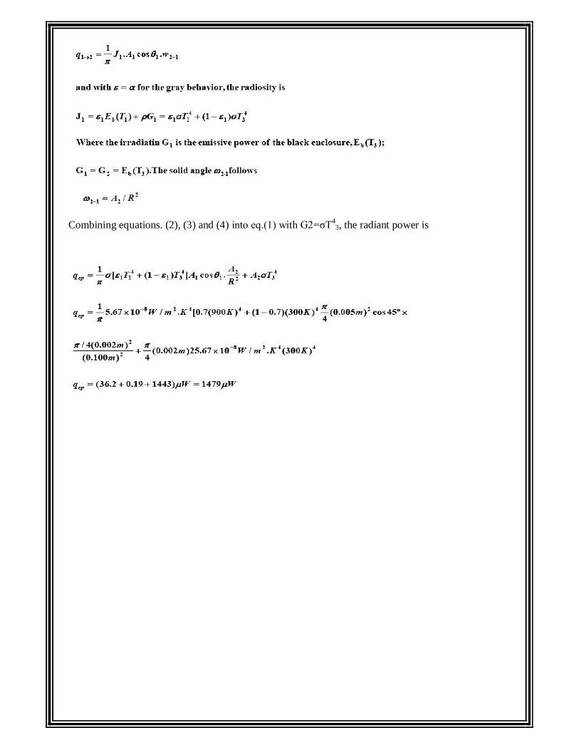
Combining equations. (2), (3) and (4) into eq.(1) with G2=σT43, the radiant power is
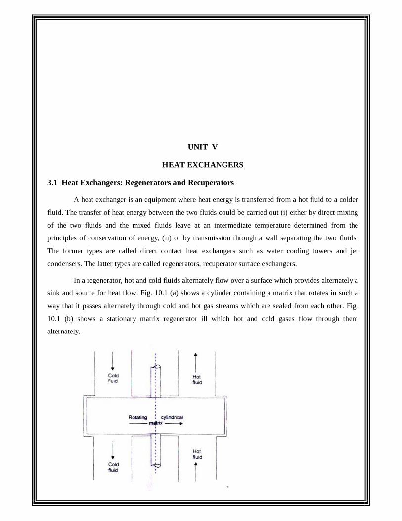
UNIT V
HEAT EXCHANGERS
3.1 Heat Exchangers: Regenerators and Recuperators
A heat exchanger is an equipment where heat energy is transferred from a hot fluid to a colder
fluid. The transfer of heat energy between the two fluids could be carried out (i) either by direct mixing
of the two fluids and the mixed fluids leave at an intermediate temperature determined from the
principles of conservation of energy, (ii) or by transmission through a wall separating the two fluids.
The former types are called direct contact heat exchangers such as water cooling towers and jet
condensers. The latter types are called regenerators, recuperator surface exchangers.
In a regenerator, hot and cold fluids alternately flow over a surface which provides alternately a
sink and source for heat flow. Fig. 10.1 (a) shows a cylinder containing a matrix that rotates in such a
way that it passes alternately through cold and hot gas streams which are sealed from each other. Fig.
10.1 (b) shows a stationary matrix regenerator ill which hot and cold gases flow through them
alternately.
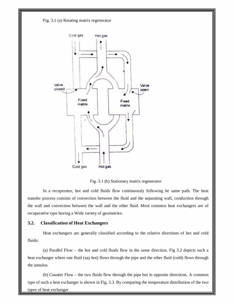
Fig. 3.1 (a) Rotating matrix regenerator
Fig. 3.1 (b) Stationary matrix regenerator
In a recuperator, hot and cold fluids flow continuously following he same path. The heat
transfer process consists of convection between the fluid and the separating wall, conduction through
the wall and convection between the wall and the other fluid. Most common heat exchangers are of
recuperative type having a Wide variety of geometries:
3.2. Classification of Heat Exchangers
Heat exchangers are generally classified according to the relative directions of hot and cold
fluids:
(a) Parallel Flow – the hot and cold fluids flow in the same direction. Fig 3.2 depicts such a
heat exchanger where one fluid (say hot) flows through the pipe and the other fluid (cold) flows through
the annulus.
(b) Counter Flow – the two fluids flow through the pipe but in opposite directions. A common
type of such a heat exchanger is shown in Fig. 3.3. By comparing the temperature distribution of the two
types of heat exchanger
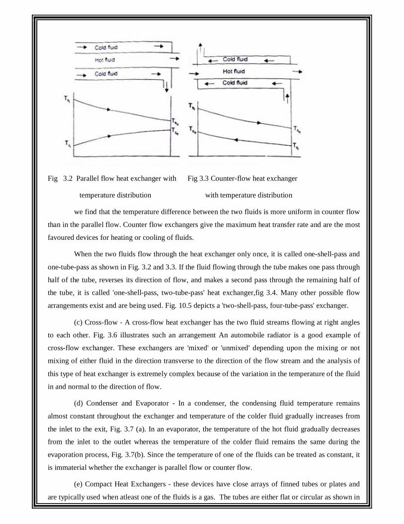
Fig 3.2 Parallel flow heat exchanger with Fig 3.3 Counter-flow heat exchanger
temperature distribution with temperature distribution
we find that the temperature difference between the two fluids is more uniform in counter flow
than in the parallel flow. Counter flow exchangers give the maximum heat transfer rate and are the most
favoured devices for heating or cooling of fluids.
When the two fluids flow through the heat exchanger only once, it is called one-shell-pass and
one-tube-pass as shown in Fig. 3.2 and 3.3. If the fluid flowing through the tube makes one pass through
half of the tube, reverses its direction of flow, and makes a second pass through the remaining half of
the tube, it is called 'one-shell-pass, two-tube-pass' heat exchanger,fig 3.4. Many other possible flow
arrangements exist and are being used. Fig. 10.5 depicts a 'two-shell-pass, four-tube-pass' exchanger.
(c) Cross-flow - A cross-flow heat exchanger has the two fluid streams flowing at right angles
to each other. Fig. 3.6 illustrates such an arrangement An automobile radiator is a good example of
cross-flow exchanger. These exchangers are 'mixed' or 'unmixed' depending upon the mixing or not
mixing of either fluid in the direction transverse to the direction of the flow stream and the analysis of
this type of heat exchanger is extremely complex because of the variation in the temperature of the fluid
in and normal to the direction of flow.
(d) Condenser and Evaporator - In a condenser, the condensing fluid temperature remains
almost constant throughout the exchanger and temperature of the colder fluid gradually increases from
the inlet to the exit, Fig. 3.7 (a). In an evaporator, the temperature of the hot fluid gradually decreases
from the inlet to the outlet whereas the temperature of the colder fluid remains the same during the
evaporation process, Fig. 3.7(b). Since the temperature of one of the fluids can be treated as constant, it
is immaterial whether the exchanger is parallel flow or counter flow.
(e) Compact Heat Exchangers - these devices have close arrays of finned tubes or plates and
are typically used when atleast one of the fluids is a gas. The tubes are either flat or circular as shown in
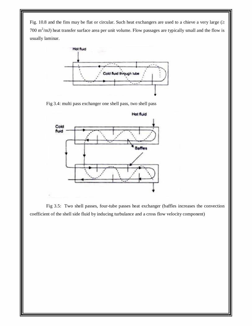
Fig. 10.8 and the fins may be flat or circular. Such heat exchangers are used to a chieve a very large (
700 m2/mJ) heat transfer surface area per unit volume. Flow passages are typically small and the flow is
usually laminar.
Fig 3.4: multi pass exchanger one shell pass, two shell pass
Fig 3.5: Two shell passes, four-tube passes heat exchanger (baffles increases the convection
coefficient of the shell side fluid by inducing turbulance and a cross flow velocity component)
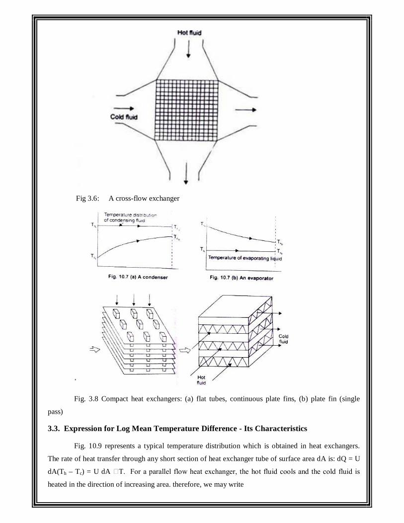
Fig 3.6: A cross-flow exchanger
Fig. 3.8 Compact heat exchangers: (a) flat tubes, continuous plate fins, (b) plate fin (single
pass)
3.3. Expression for Log Mean Temperature Difference - Its Characteristics
Fig. 10.9 represents a typical temperature distribution which is obtained in heat exchangers.
The rate of heat transfer through any short section of heat exchanger tube of surface area dA is: dQ = U
dA(Th – Tc) = U dA T. For a parallel flow heat exchanger, the hot fluid cools and the cold fluid is
heated in the direction of increasing area. therefore, we may write
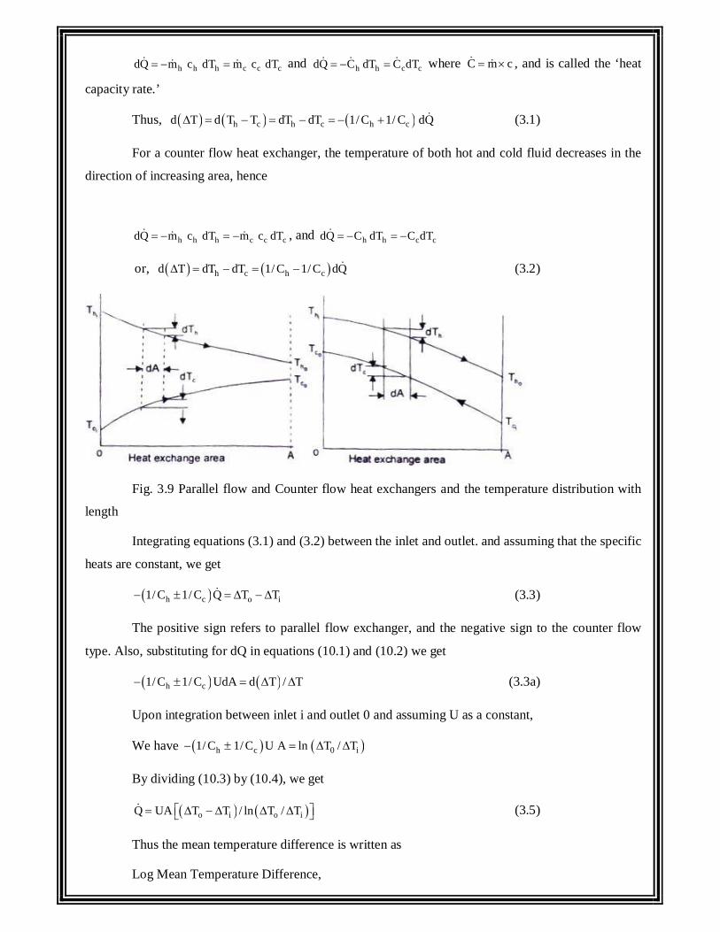
h h h c c cdQ m c dT m c dT and h h c cdQ C dT C dT where C m c , and is called the ‘heat
capacity rate.’
Thus, h c h c h cd T d T T dT dT 1/ C 1/ C dQ (3.1)
For a counter flow heat exchanger, the temperature of both hot and cold fluid decreases in the
direction of increasing area, hence
h h h c c cdQ m c dT m c dT , and h h c cdQ C dT C dT
or, h c h cd T dT dT 1/ C 1/ C dQ (3.2)
Fig. 3.9 Parallel flow and Counter flow heat exchangers and the temperature distribution with
length
Integrating equations (3.1) and (3.2) between the inlet and outlet. and assuming that the specific
heats are constant, we get
h c o i1/ C 1/ C Q T T (3.3)
The positive sign refers to parallel flow exchanger, and the negative sign to the counter flow
type. Also, substituting for dQ in equations (10.1) and (10.2) we get
h c1/ C 1/ C UdA d T / T (3.3a)
Upon integration between inlet i and outlet 0 and assuming U as a constant,
We have h c 0 i1/ C 1/ C U A ln T / T
By dividing (10.3) by (10.4), we get
o i o iQ UA T T / ln T / T (3.5)
Thus the mean temperature difference is written as
Log Mean Temperature Difference,
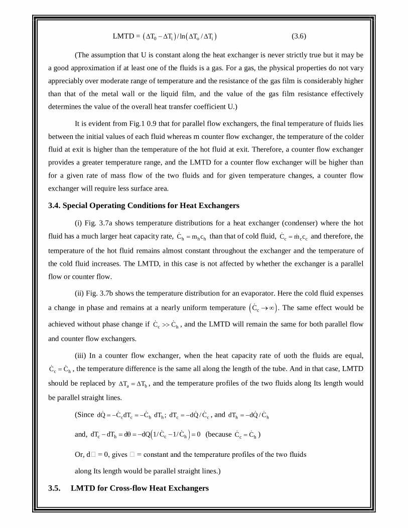
LMTD = 0 i o iT T / ln T / T (3.6)
(The assumption that U is constant along the heat exchanger is never strictly true but it may be
a good approximation if at least one of the fluids is a gas. For a gas, the physical properties do not vary
appreciably over moderate range of temperature and the resistance of the gas film is considerably higher
than that of the metal wall or the liquid film, and the value of the gas film resistance effectively
determines the value of the overall heat transfer coefficient U.)
It is evident from Fig.1 0.9 that for parallel flow exchangers, the final temperature of fluids lies
between the initial values of each fluid whereas m counter flow exchanger, the temperature of the colder
fluid at exit is higher than the temperature of the hot fluid at exit. Therefore, a counter flow exchanger
provides a greater temperature range, and the LMTD for a counter flow exchanger will be higher than
for a given rate of mass flow of the two fluids and for given temperature changes, a counter flow
exchanger will require less surface area.
3.4. Special Operating Conditions for Heat Exchangers
(i) Fig. 3.7a shows temperature distributions for a heat exchanger (condenser) where the hot
fluid has a much larger heat capacity rate, h h hC m c than that of cold fluid, c c cC m c and therefore, the
temperature of the hot fluid remains almost constant throughout the exchanger and the temperature of
the cold fluid increases. The LMTD, in this case is not affected by whether the exchanger is a parallel
flow or counter flow.
(ii) Fig. 3.7b shows the temperature distribution for an evaporator. Here the cold fluid expenses
a change in phase and remains at a nearly uniform temperature cC . The same effect would be
achieved without phase change if c hC C , and the LMTD will remain the same for both parallel flow
and counter flow exchangers.
(iii) In a counter flow exchanger, when the heat capacity rate of uoth the fluids are equal,
c hC C , the temperature difference is the same all along the length of the tube. And in that case, LMTD
should be replaced by a bT T , and the temperature profiles of the two fluids along Its length would
be parallel straight lines.
(Since c c h h c cdQ C dT C dT ; dT dQ / C , and h hdT dQ / C
and, c h c hdT dT d dQ 1/ C 1/ C 0 (because c hC C )
Or, d = 0, gives = constant and the temperature profiles of the two fluids
along Its length would be parallel straight lines.)
3.5. LMTD for Cross-flow Heat Exchangers
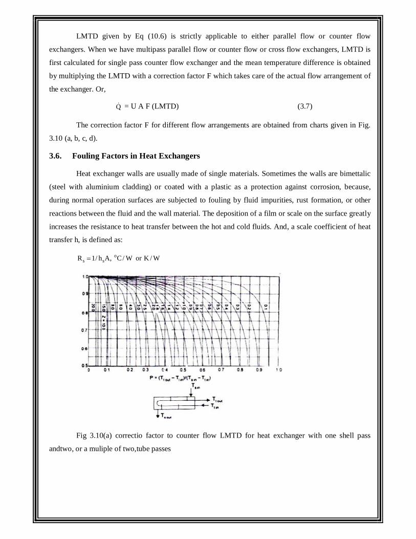
LMTD given by Eq (10.6) is strictly applicable to either parallel flow or counter flow
exchangers. When we have multipass parallel flow or counter flow or cross flow exchangers, LMTD is
first calculated for single pass counter flow exchanger and the mean temperature difference is obtained
by multiplying the LMTD with a correction factor F which takes care of the actual flow arrangement of
the exchanger. Or,
Q = U A F (LMTD) (3.7)
The correction factor F for different flow arrangements are obtained from charts given in Fig.
3.10 (a, b, c, d).
3.6. Fouling Factors in Heat Exchangers
Heat exchanger walls are usually made of single materials. Sometimes the walls are bimettalic
(steel with aluminium cladding) or coated with a plastic as a protection against corrosion, because,
during normal operation surfaces are subjected to fouling by fluid impurities, rust formation, or other
reactions between the fluid and the wall material. The deposition of a film or scale on the surface greatly
increases the resistance to heat transfer between the hot and cold fluids. And, a scale coefficient of heat
transfer h, is defined as:
os sR 1/ h A, C/ W or K / W
Fig 3.10(a) correctio factor to counter flow LMTD for heat exchanger with one shell pass
andtwo, or a muliple of two,tube passes
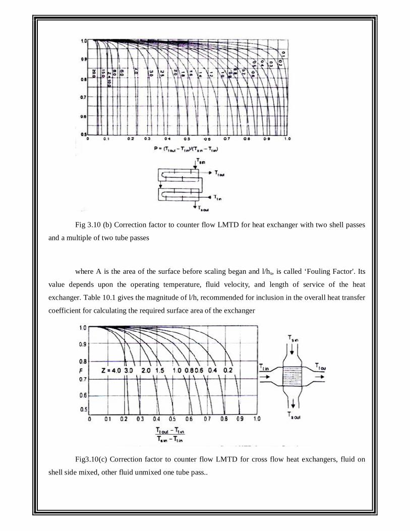
Fig 3.10 (b) Correction factor to counter flow LMTD for heat exchanger with two shell passes
and a multiple of two tube passes
where A is the area of the surface before scaling began and l/hs, is called ‘Fouling Factor'. Its
value depends upon the operating temperature, fluid velocity, and length of service of the heat
exchanger. Table 10.1 gives the magnitude of l/h, recommended for inclusion in the overall heat transfer
coefficient for calculating the required surface area of the exchanger
Fig3.10(c) Correction factor to counter flow LMTD for cross flow heat exchangers, fluid on
shell side mixed, other fluid unmixed one tube pass..
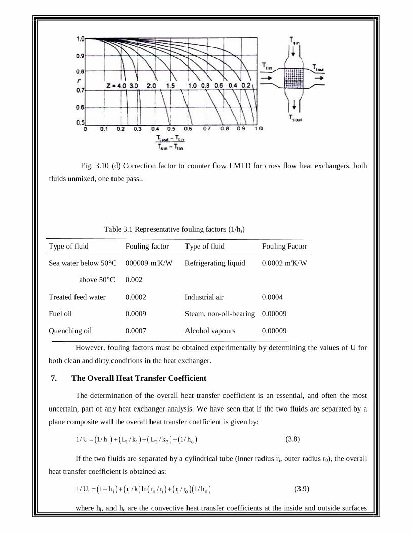
Fig. 3.10 (d) Correction factor to counter flow LMTD for cross flow heat exchangers, both
fluids unmixed, one tube pass..
Table 3.1 Representative fouling factors (1/hs)
Type of fluid Fouling factor Type of fluid Fouling Factor
Sea water below 50°C 000009 m'K/W Refrigerating liquid 0.0002 m'K/W
above 50°C 0.002
Treated feed water 0.0002 Industrial air 0.0004
Fuel oil 0.0009 Steam, non-oil-bearing 0.00009
Quenching oil 0.0007 Alcohol vapours 0.00009
However, fouling factors must be obtained experimentally by determining the values of U for
both clean and dirty conditions in the heat exchanger.
7. The Overall Heat Transfer Coefficient
The determination of the overall heat transfer coefficient is an essential, and often the most
uncertain, part of any heat exchanger analysis. We have seen that if the two fluids are separated by a
plane composite wall the overall heat transfer coefficient is given by:
i 1 1 2 2 o1/ U 1/ h L / k L / k 1/ h (3.8)
If the two fluids are separated by a cylindrical tube (inner radius ri, outer radius r0), the overall
heat transfer coefficient is obtained as:
i i i o i i o o1/ U 1 h r / k ln r / r r / r 1/ h (3.9)
where hi, and ho are the convective heat transfer coefficients at the inside and outside surfaces
and V, is the overall heat transfer coefficient based on the inside surface area. Similarly, for the outer
surface area, we have:
o o o o i o i i1/ U 1/ h r / k ln r r r r 1/ h (3.10)
and i iU A will be equal to o oU A ; or, i i o oU r U r .
The effect of scale formation on the inside and outside surfaces of the tubes of a heat exchanger
would be to introduce two additional thermal resistances to the heat flow path. If hsi and hso are the two
heat transfer coefficients due to scale formation on the inside and outside surface of the inner pipe, the
rate of heat transfer is given by
i o i i si i o i so o o oQ T T / 1/ h A 1/ h A ln r r / 2 Lk 1/ h A 1/ h A (3.11)
where Ti, and To are the temperature of the fluid at the inside and outside of the tube. Thus, the
overall heat transfer coeffiCIent based on the inside and outside surface area of the tube would be:
i i si i o i i o so i o o1/ U 1/ h 1/ h r / k ln r / r r / r 1/ h r / r 1/ h ; (3.12)
and
o o i i o i si o i 0 so o1/ U r / r 1/ h r / r 1/ h ln r / r r / k 1/ h 1/ h
Example 3.1 In a parallel flow heat exchanger water flows through the inner pipe and is heated from
25°C to 75°C. Oil flowing through the annulus is cooled from 210°C to 110°C. It is
desired to cool the oil to a lower temperature by increasing the length of the tube. Estimate
the minimum temperature to which the oil can be cooled.
Solution: By making an energy balance, heat received by water must be equal to 4he heat
given out by oil.
w w o o w om c 75 25 m c 210 110 ;C / C 100 / 50 2.0
In a parallel flow heat exchanger, the minimum temperature to which oil can be cooled will be
equal to the maximum temperature to which water can be heated,
Fig. 10.2: ho coT T
therefore, Cw (T –25) = Co (210 – T);
(T – 25)/(210 – T) = 1/2 = 0.5; or, T = 260/3 = 86.67°C.
or the same capacity rates the oil can be cooled to 25°C (equal to the water inlet temperature) in
a counter-flow arrangement.
Example 3.2 Water at the rate of 1.5 kg/s IS heated from 30°C to 70°C by an oil (specific heat 1.95
kJ/kg C). Oil enters the exchanger at 120°C and leaves the exchanger at 80°C. If the
overall heat transfer coefficient remains constant at 350 W /m2°C, calculate the heat
exchange area for (i) parallel-flow, (ii) counter-flow, and (iii) cross-flow arrangement.
Solution: Energy absorbed by water,
w wQ m c T 1.5 4.182 40 250.92 kW
(i) Parallel flow: Fig. 10.9; a bT 120 30 90; T 80 70 10
LMTD = (90 – 10)/ln(90/10) = 36.4;
Area = Q/U (LMTD) = 250920 /(350 × 36.4) = 19.69 m2.
(ii) Counter flow: Fig 10.9; Ta. = 120 – 70 = 50, Tb = 80 – 30 = 50
Since Ta. = Tb,. LMTD should be replaced by T = 50
Area A = 2Q / U T 250920 / 350 50 14.33 m
(iii) Cross flow: assuming both fluids unmixed - Fig. 10.10d
using the nomenclature of the figure and assuming that water flows through the tubes and oil
flows through the shell,
to ti si tiP T T / T T 70 30 / 120 30 0.444
si so to tiZ T T / T T 120 80 / 70 30 1.0
and the correction factor, F = 0.93
Q UAF T ; or Area A = 250920/(350 × 0.93 × 50) = 15.41 m2.
Example 3.3 0.5 kg/s of exhaust gases flowing through a heat exchanger are cooled from 400°C to
120°C by water initially at 25°C. The specific heat capacities of exhaust gases and water
are 1.15 and 4.19 kJ/kgK respectively, and the overall heat transfer coefficient from
gases to water is 150 W/m2K. If the cooling water flow rate is 0.7 kg/s, calculate the
surface area when (i) parallel-flow (ii) cross-flow with exhaust gases flowing through
tubes and water is mixed in the shell.
Solution: The heat given out by the exhaust gases is equal to the heat gained by water.
or, 0.5 × 1.15 × (400 – 120) = 0.7 × 4.19 × (T – 25)
Therefore, the temperature of water at exit, T = 79.89°C
For paralle1-flow: aT 400 25 375; bT 120 79.89 40.11
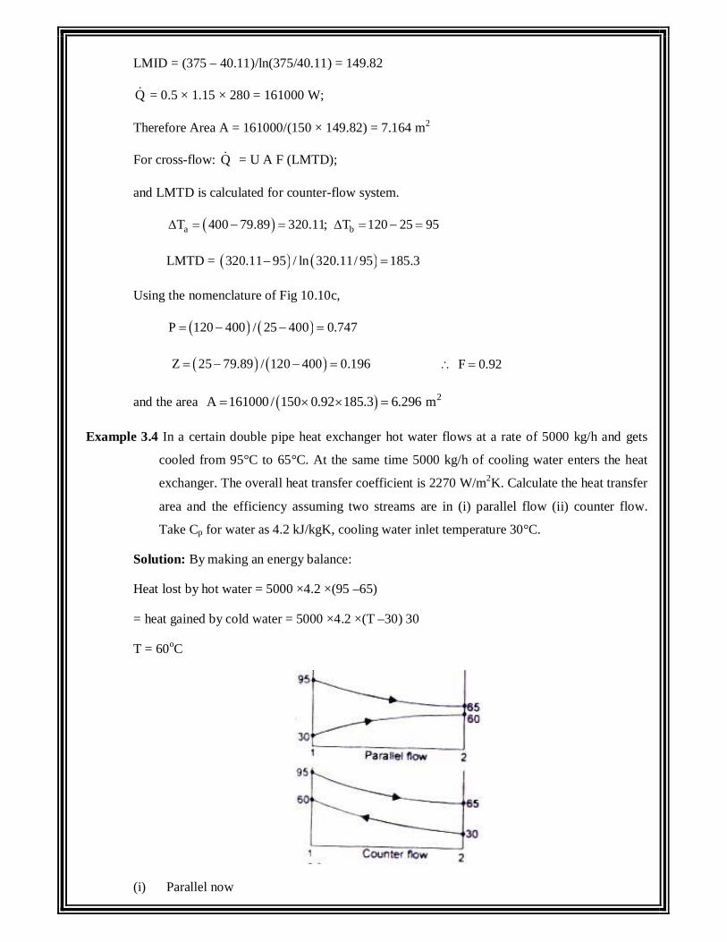
LMID = (375 – 40.11)/ln(375/40.11) = 149.82
Q = 0.5 × 1.15 × 280 = 161000 W;
Therefore Area A = 161000/(150 × 149.82) = 7.164 m2
For cross-flow: Q = U A F (LMTD);
and LMTD is calculated for counter-flow system.
a bT 400 79.89 320.11; T 120 25 95
LMTD = 320.11 95 / ln 320.11/ 95 185.3
Using the nomenclature of Fig 10.10c,
P 120 400 / 25 400 0.747
Z 25 79.89 / 120 400 0.196 F 0.92
and the area 2A 161000 / 150 0.92 185.3 6.296 m
Example 3.4 In a certain double pipe heat exchanger hot water flows at a rate of 5000 kg/h and gets
cooled from 95°C to 65°C. At the same time 5000 kg/h of cooling water enters the heat
exchanger. The overall heat transfer coefficient is 2270 W/m2K. Calculate the heat transfer
area and the efficiency assuming two streams are in (i) parallel flow (ii) counter flow.
Take Cp for water as 4.2 kJ/kgK, cooling water inlet temperature 30°C.
Solution: By making an energy balance:
Heat lost by hot water = 5000 ×4.2 ×(95 –65)
= heat gained by cold water = 5000 ×4.2 ×(T –30) 30
T = 60oC
(i) Parallel now
1 95 30 65
2 65 60 5
LMTD = 65 5 / ln 65 / 5 23.4
Area, 3
2500 4.2 10 30A Q / U LMTD 3.295 m3600 2270 23.4
(ii) Counter flow: 1 = (95 – 60) = 35
2 = (65 – 30) = 35
LMTD = T = 35
Area A = 500 × 4200 × 30/(3600 × 2270 × 35) = 2.2 m2
, Efficiency.= Actual heat transferred/Maximum heat that could be transferred. Therefore, for
parallel flow, = (95 – 65)/(95 – 60) = 0.857
For counter flow, = (95 - 65)/(95 – 30) = 0.461.
Counter now
Example 3.5 The flow rates of hot and cold water streams running through a double pipe heat
exchanger (inside and outside diameter of the tube 80 mm and 100 mm) are 2 kg/s and 4
kg/so The hot fluid enters at 75°C and comes out at 45oC. The cold fluid enters at 20°C.
If the convective heat transfer at the inside and outside surface of the tube is 150 and 180
W /m2K, thermal conductivity of the tube material 40 W/mK, calculate the area of the
heat exchanger assuming counter flow.
Solution: Let T is the temperature of the cold water at outlet.
By making an energy balance, h h h1 h2 c c c2 c1Q m c T T m c T T
since oh cc c , 4.2 kJ / kgK; 2 75 45 4 T 20 ; T 35 C
and Q 252 kW
for counter flow: 1 275 35 40; 45 20 25
LMTD = (40 – 25) / ln (40/25) = 31.91
overall heat transfer coefficient based in the inside surface of tube
i i o i o i o1/ U 1/ h r / k ln r / r r r 1/ h
1/150 0.04 / 40 ln 50 / 40 50 / 40 1/180 0.0138
and U = 72.28
area 3 2A Q / U LMTD 252 10 / 72.28 31.91 109.26 m
Example 3.6 Water flows through a copper tube (k = 350 W/mK, inner and outer diameter 2.0 cm
and 2.5 cm respectively) of a double pipe heat exchanger. Oil flows through the
annulus between this pipe and steel pipe. The convective heat transfer coefficient on
the inside and outside of the copper tube are 5000 and 1500 W /m2K. The fouling
factors on the water and oil sides are 0.0022 and 0.00092 K1W. Calculate the overall
heat transfer coefficient with and without the fouling factor.
Solution: The scales formed on the inside and outside surface of the copper tube introduces
two additional resistances in the heat flow path. Resistance due to inside convective heat transfer
coefficient
i i i1/ h A 1/ 5000 A
Resistance due to scale formation on the inside = 1/hsAi = 0.0022
Resistance due to conduction through the tube wall = o iln r / r / 2 Lk
4ln 2.5 / 2.0 / 2 L 350 1.014 10 / L
Resistance due to convective heat transfer on the outside
o o o1/ h A 1/1500A
Resistance due to scale formation on the outside = s o1/ h A 0.00092
Since, i 1 i iQ T R U A T T / 1/ U A ; we have
(a) With fouling factor:-
Overall heat transfer coefficient based on the inside pipe surface
4 4iU 1/ 1/ 5000 0.02 0.0022 0.00092 0.02 1.014 10 8.33 10
= 809.47 W/m2K per metre length of pipe
(b) Without fouling factor
4 4iU 1/ 1/ 5000 0.02 1.014 10 8.33 10
= 962.12 W/m2K per m of pipe length.
The heat transfer rate will reduce by (962.12 – 809.47)1962.12 = 15.9 percent when fouling
factor is considered.
Example 3.7 In a surface condenser, dry and saturated steam at 50oC enters at the rate of 1 kg/so The
circulating water enters the tube, (25 nun inside diameter, 28 mm outside diameter, k =
300 W/mK) at a velocity of
2 m/s. If the convective heat transfer coefficient on the outside surface of the tube is
5500 W/m2K, the inlet and outlet temperatures of water are 25oC and 35oC respectively,
calculate the required surface area.
Solution: For calculating the convective heat transfer coefficient on the inside surface of the
tube, we calculate the Reynolds number on the basis of properties of water at the mean temperature of
30oC. The properties are:
= 0.001 Pa-s, = 1000 kg/m3, k = 0.6 W/mK, hfg at 50oC = 2375 kJ/kg
Re = VD/ = 103 × 2 × 0.025/0.001 = 50,000, a turbulent flow. Pr = 7.0.
The heat transfer coefficient at the inside surface can be calculated by:
Nu = 0.023 Re0.8 8 Pr0.3 = 0.023 (50000)0.8 (7)0.3 = 236.828
and hi = 236.828 × 0.6/0.025 = 5684 W/m2K.
The overall heat transfer coefficient based on the outer diameter,
U = 1/(0.028/(0.025 × 5684) + 1/5500 + 0.014 ln(28/25)/300)
= 2603.14 W/m2K
Ta. = (50 - 25) = 25; Tb = (50 - 35) = 15;
LMTD = (25 -15)/ln(25/15) = 19.576.
Assuming one shell pass and one tube pass, Q = UA (LMTD)
or A = 2375 × 103/(2603.14 x 19.576) = 46.6 m2
Mass of Circulating water = Q/(cp T) = 2375/(4.182 × 10) = 56.79 kg/s
also, mw = × area × V × n, where n is the number of tubes.
n = 56.79 × 4/(2 × × 0.025 × 0.025 × 1000) = 58 tubes
Surface area, 46.6 = n × × d × L
and L = 46.6/(58 × × 0.025) = 10.23 m.
Hence more than one pass should be used.
Example 3.8 A heat exchanger is used to heat water from 20°C to 50°C when thin walled water tubes
(inner diameter 25 mm, length IS m) are laid beneath a hot spring water pond,
temperature 75°C. Water flows through the tubes with a velocity of 1 m/s. Estimate the
required overall heat transfer coefficient and the convective heat transfer coefficient at
the outer surface of the tube.
Solution: Water flow rate, m = × V × A = 103 × 1 × ( /4) (0.025)2
= 0.49 kg/so
Heat transferred to water, Q = m c ( T) = 0.49 × 4200 × 30 = 61740 W.
Since the temperature of the water in the hot spring is constant,
1 275 20 55; 75 50 25 ;
LMTD = (55 – 25) / ln(55/25) = 38
Overall heat transfer coefficient, U = Q/ (A × LMTD)
= 61740/(38 × × 0.025 × 15) = 1378.94 W/m2K.
The properties of water at the mean temperature (20 + 50)/2 = 35°C are:
0.001 Pa s, k 0.6 W / mk and Pr = 7.0
Reynolds number, Re Vd / 1000 1.0 0.25 / 0.001 25000 , turbulent flow.
Nu = 0.023 (Re)0.8 (Pr)0.33 = 0.023 (25000)0.8 × (7)0.33 = 144.2
and hi = 144.2 × k/d = 144.2 × 0.6/0.025 = 3460.8 W/m2K
Neglecting the resistance of the thin tube wall,
1/U = 1/hi + 1/ho; o1/ h 1/1378.94 1/ 3460.8
or, 2oh 2292.3 W / m K
Example 3.9 A hot fluid at 200°C enters a heat exchanger at a mass rate of 10000 kg/h. Its specific
heat is 2000 J/kg K. It is to be cooled by another fluid entering at 25°C with a mass
flow rate 2500 k g/h and specific heat 400 J/kgK. The overall heat transfer coefficient
based on outside area of 20 m2 is 250 W/m2K. Find the exit temperature of the hot
fluid when the fluids are in parallel flow.
Solution: From Eq(10.3a), h cU dA 1/ C 1/ C d T / T
Upon integration,
2h c 1U A 1/ C 1/ C ln T | 0 0 i ih c h cln T T / T T
The values are: U = 250 W/m2K
A = 20 m2
l/Ch = 3600/(10000 × 2000) = 1.8 × 10⁻⁴
1/Cc = 3600/(2500 × 400) = 3.6 × 10⁻³
–UA(1/Ch + l/Cc) = –250 × 20 (1.8 × 10⁻⁴ + 3.6 × 10⁻³) = -18.9
; or, 0 0h cT T
By making an energy balance,
0 0h c10000 2000 200 T 2500 400 T 25
0h2500 400 T 25 and 0h21 T 20 200 25
or, 0
ohT 191.67 C
Example 3.10 Cold water at the rate of 4 kg/s is heated from 30°C to 50°C in a shell and tube heat
exchanger with hot water entering at 95°C at a rate of 2 kg/s. The hot water flows
through the shell. The cold water flows through tubes 2 cm inner diameter, velocity of
flow 0.38 m/s. Calculate the number 0 f tube passes, the number 0 f tubes per pass if the
maximum length of the tube is limited to 2.0 m and the overall heat transfer coefficient
is 1420 W/m2K.
Solution: Let T be the temperature of the hot water at exit. By making an energy balance:
4c 50 30 2c 95 T ; oT 55 C
For a counter-flow arrangement:
aT 95 50 45 , bT 55 30 25 ,
LMTD 45 25 / ln 45 / 25 34; Q mC T 4 4.182 20 334.56 kW
Since the cold water is flowing through the tubes, the number of tubes, n is given by
m n Area × velocity; the cross-sectional area 3.142 × 10⁻² m2
4 = n × 1000 × 3.142 × 10–4 × 0.38; n = 33.5, or 34 (say)
Assuming one shell and two tube pass, we use Fig. 10.9(a).
P 50 30 / 95 30 0.3 ; Z 95 55 / 50 30 2.0
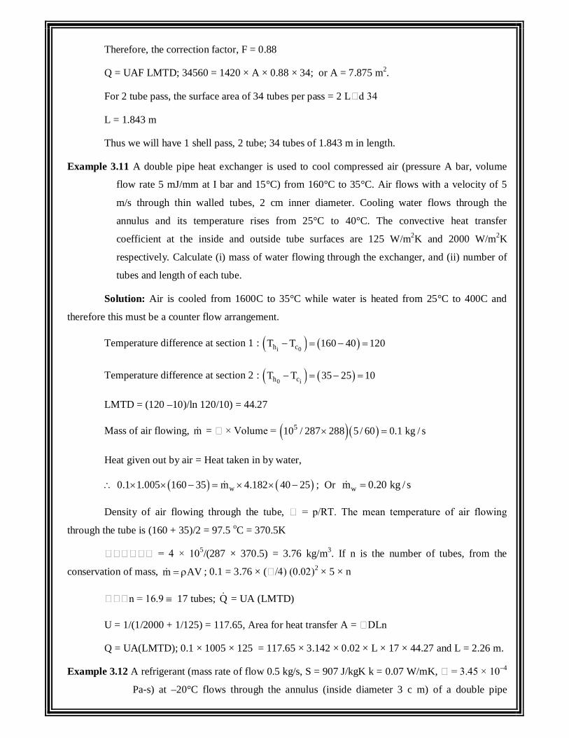
Therefore, the correction factor, F = 0.88
Q = UAF LMTD; 34560 = 1420 × A × 0.88 × 34; or A = 7.875 m2.
For 2 tube pass, the surface area of 34 tubes per pass = 2 L d 34
L = 1.843 m
Thus we will have 1 shell pass, 2 tube; 34 tubes of 1.843 m in length.
Example 3.11 A double pipe heat exchanger is used to cool compressed air (pressure A bar, volume
flow rate 5 mJ/mm at I bar and 15°C) from 160°C to 35°C. Air flows with a velocity of 5
m/s through thin walled tubes, 2 cm inner diameter. Cooling water flows through the
annulus and its temperature rises from 25°C to 40°C. The convective heat transfer
coefficient at the inside and outside tube surfaces are 125 W/m2K and 2000 W/m2K
respectively. Calculate (i) mass of water flowing through the exchanger, and (ii) number of
tubes and length of each tube.
Solution: Air is cooled from 1600C to 35°C while water is heated from 25°C to 400C and
therefore this must be a counter flow arrangement.
Temperature difference at section 1 : i 0h cT T 160 40 120
Temperature difference at section 2 : 0 ih cT T 35 25 10
LMTD = (120 –10)/ln 120/10) = 44.27
Mass of air flowing, m = × Volume = 510 / 287 288 5 / 60 0.1 kg / s
Heat given out by air = Heat taken in by water,
w0.1 1.005 160 35 m 4.182 40 25 ; Or wm 0.20 kg / s
Density of air flowing through the tube, = p/RT. The mean temperature of air flowing
through the tube is (160 + 35)/2 = 97.5 oC = 370.5K
= 4 × 10⁵/(287 × 370.5) = 3.76 kg/m3. If n is the number of tubes, from the
conservation of mass, m AV ; 0.1 = 3.76 × ( /4) (0.02)2 × 5 × n
n = 16.9 17 tubes; Q = UA (LMTD)
U = 1/(1/2000 + 1/125) = 117.65, Area for heat transfer A = DLn
Q = UA(LMTD); 0.1 × 1005 × 125 = 117.65 × 3.142 × 0.02 × L × 17 × 44.27 and L = 2.26 m.
Example 3.12 A refrigerant (mass rate of flow 0.5 kg/s, S = 907 J/kgK k = 0.07 W/mK, = 3.45 × 10⁻⁴
Pa-s) at –20°C flows through the annulus (inside diameter 3 c m) of a double pipe
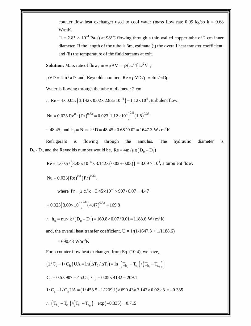
counter flow heat exchanger used to cool water (mass flow rate 0.05 kg/so k = 0.68
W/mK,
= 2.83 × 10⁻⁴ Pa-s) at 98°C flowing through a thin walled copper tube of 2 cm inner
diameter. If the length of the tube is 3m, estimate (i) the overall heat transfer coefficient,
and (ii) the temperature of the fluid streams at exit.
Solution: Mass rate of flow, m AV = 2/ 4 D V ;
VD 4 m / D and, Reynolds number, Re VD / 4m / D
Water is flowing through the tube of diameter 2 cm,
4 4Re 4 0.05 / 3.142 0.02 2.83 10 1.12 10 , turbulent flow.
0.80.33 0.330.8 4Nu 0.023 Re Pr 0.023 1.12 10 1.8
= 48.45; and 2ih Nu k / D 48.45 0.68 / 0.02 1647.3 W / m K
Refrigerant is flowing through the annulus. The hydraulic diameter is
Do - Di, and the Reynolds number would be, 0 iRe 4m / D D
4Re 4 0.5 / 3.45 10 3.142 0.02 0.03 = 3.69 × 10⁴, a turbulent flow.
0.8 0.33Nu 0.023 Re Pr ,
where 4Pr c / k 3.45 10 907 / 0.07 4.47
0.8 0.3340.023 3.69 10 4.47 169.8
2o o ih nu k / D D 169.8 0.07 / 0.01 1188.6 W / m K
and, the overall heat transfer coefficient, U = 1/(1/1647.3 + 1/1188.6)
= 690.43 W/m2K
For a counter flow heat exchanger, from Eq. (10.4), we have,
0 i i 0c h 0 i h c h c1/ C 1/ C UA ln T / T ln T T / T T
cC 0.5 907 453.5 ; hC 0.05 4182 209.1
c h1/ C 1/ C UA 1/ 453.5 1/ 209.1 690.43 3.142 0.02 3 = –0.335
0 i i 0h c h cT T / T T exp 0.335 0.715
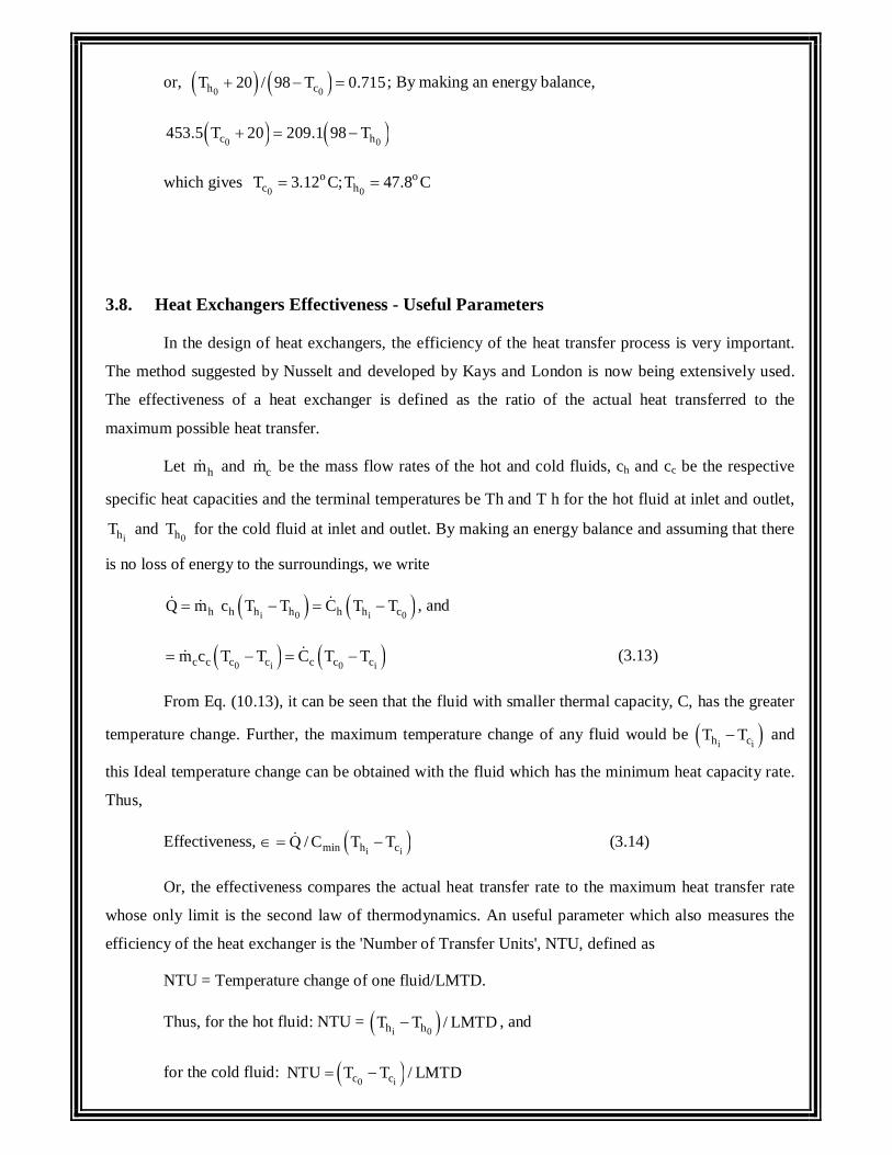
or, 0 0h cT 20 / 98 T 0.715 ; By making an energy balance,
0 0c h453.5 T 20 209.1 98 T
which gives 0 0
o oc hT 3.12 C;T 47.8 C
3.8. Heat Exchangers Effectiveness - Useful Parameters
In the design of heat exchangers, the efficiency of the heat transfer process is very important.
The method suggested by Nusselt and developed by Kays and London is now being extensively used.
The effectiveness of a heat exchanger is defined as the ratio of the actual heat transferred to the
maximum possible heat transfer.
Let hm and cm be the mass flow rates of the hot and cold fluids, ch and cc be the respective
specific heat capacities and the terminal temperatures be Th and T h for the hot fluid at inlet and outlet,
ihT and 0hT for the cold fluid at inlet and outlet. By making an energy balance and assuming that there
is no loss of energy to the surroundings, we write
i 0 i 0h h h h h h cQ m c T T C T T , and
0 i 0 ic c c c c c cm c T T C T T (3.13)
From Eq. (10.13), it can be seen that the fluid with smaller thermal capacity, C, has the greater
temperature change. Further, the maximum temperature change of any fluid would be i ih cT T and
this Ideal temperature change can be obtained with the fluid which has the minimum heat capacity rate.
Thus,
Effectiveness, i imin h cQ / C T T (3.14)
Or, the effectiveness compares the actual heat transfer rate to the maximum heat transfer rate
whose only limit is the second law of thermodynamics. An useful parameter which also measures the
efficiency of the heat exchanger is the 'Number of Transfer Units', NTU, defined as
NTU = Temperature change of one fluid/LMTD.
Thus, for the hot fluid: NTU = i 0h hT T / LMTD , and
for the cold fluid: 0 ic cNTU T T / LMTD
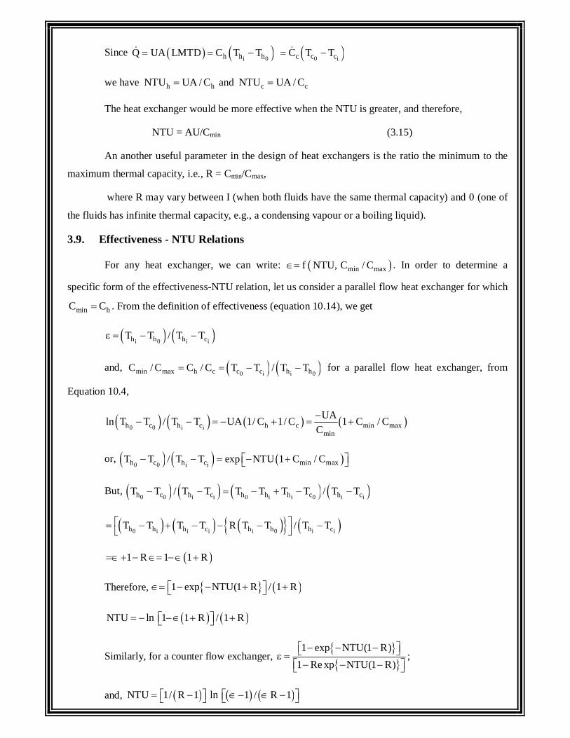
Since i 0h h hQ UA LMTD C T T 0 ic c cC T T
we have h hNTU UA / C and c cNTU UA / C
The heat exchanger would be more effective when the NTU is greater, and therefore,
NTU = AU/Cmin (3.15)
An another useful parameter in the design of heat exchangers is the ratio the minimum to the
maximum thermal capacity, i.e., R = Cmin/Cmax,
where R may vary between I (when both fluids have the same thermal capacity) and 0 (one of
the fluids has infinite thermal capacity, e.g., a condensing vapour or a boiling liquid).
3.9. Effectiveness - NTU Relations
For any heat exchanger, we can write: min maxf NTU, C / C . In order to determine a
specific form of the effectiveness-NTU relation, let us consider a parallel flow heat exchanger for which
min hC C . From the definition of effectiveness (equation 10.14), we get
i 0 i ih h h cT T / T T
and, 0 i i 0min max h c c c h hC / C C / C T T / T T for a parallel flow heat exchanger, from
Equation 10.4,
0 0 i ih c h c h c min maxmin
UAln T T / T T UA 1/ C 1/ C 1 C / CC
or, 0 0 i ih c h c min maxT T / T T exp NTU 1 C / C
But, 0 0 i i 0 i i 0 i ih c h c h h h c h cT T / T T T T T T / T T
0 i i i i 0 i ih h h c h h h cT T T T R T T / T T
1 R 1 1 R
Therefore, 1 exp NTU(1 R / 1 R
NTU ln 1 1 R / 1 R
Similarly, for a counter flow exchanger,
1 exp NTU(1 R)1 Re xp NTU(1 R)
;
and, NTU 1/ R 1 ln 1 / R 1
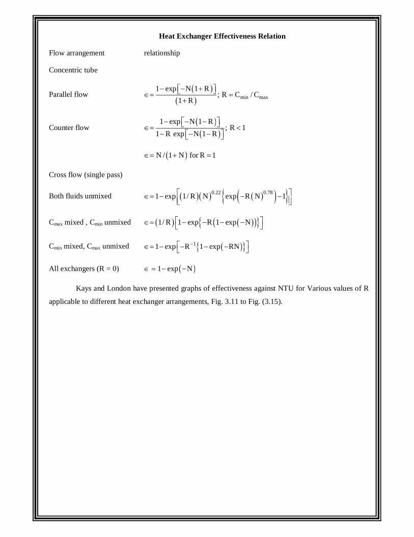
Heat Exchanger Effectiveness Relation
Flow arrangement relationship
Concentric tube
Parallel flow
min max1 exp N 1 R
; R C / C1 R
Counter flow
1 exp N 1 R; R 1
1 R exp N 1 R
N / 1 N for R 1
Cross flow (single pass)
Both fluids unmixed 0.22 0.781 exp 1/ R N exp R N 1
Cmax mixed , Cmin unmixed 1/ R 1 exp R 1 exp N
Cmin mixed, Cmax unmixed 11 exp R 1 exp RN
All exchangers (R = 0) 1 exp N
Kays and London have presented graphs of effectiveness against NTU for Various values of R
applicable to different heat exchanger arrangements, Fig. 3.11 to Fig. (3.15).
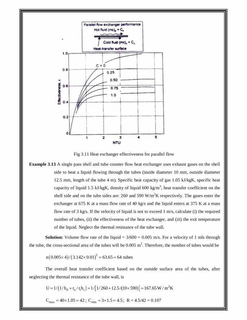
Fig 3.11 Heat exchanger effectiveness for parallel flow
Example 3.13 A single pass shell and tube counter flow heat exchanger uses exhaust gases on the shell
side to heat a liquid flowing through the tubes (inside diameter 10 mm, outside diameter
12.5 mm, length of the tube 4 m). Specific heat capacity of gas 1.05 kJ/kgK, specific heat
capacity of liquid 1.5 kJ/kgK, density of liquid 600 kg/m3, heat transfer coefficient on the
shell side and on the tube sides are: 260 and 590 W/m2K respectively. The gases enter the
exchanger at 675 K at a mass flow rate of 40 kg/s and the liquid enters at 375 K at a mass
flow rate of 3 kg/s. If the velocity of liquid is not to exceed 1 m/s, calculate (i) the required
number of tubes, (ii) the effectiveness of the heat exchanger, and (iii) the exit temperature
of the liquid. Neglect the thermal resistance of the tube wall.
Solution: Volume flow rate of the liquid = 3/600 = 0.005 m/s. For a velocity of 1 mls through
the tube, the cross-sectional area of the tubes will be 0.005 m2. Therefore, the number of tubes would be
2n 0.005 4 / 3.142 0.01 63.65 64 tubes
The overall heat transfer coefficient based on the outside surface area of the tubes, after
neglecting the thermal resistance of the tube wall, is
20 o i iU 1/ 1/ h r / r h 1/ 1/ 260 12.5 /(10 590) 167.65W / m K
maxC 40 1.05 42 ; minC 3 1.5 4.5 ; R = 4.5/42 = 0.107
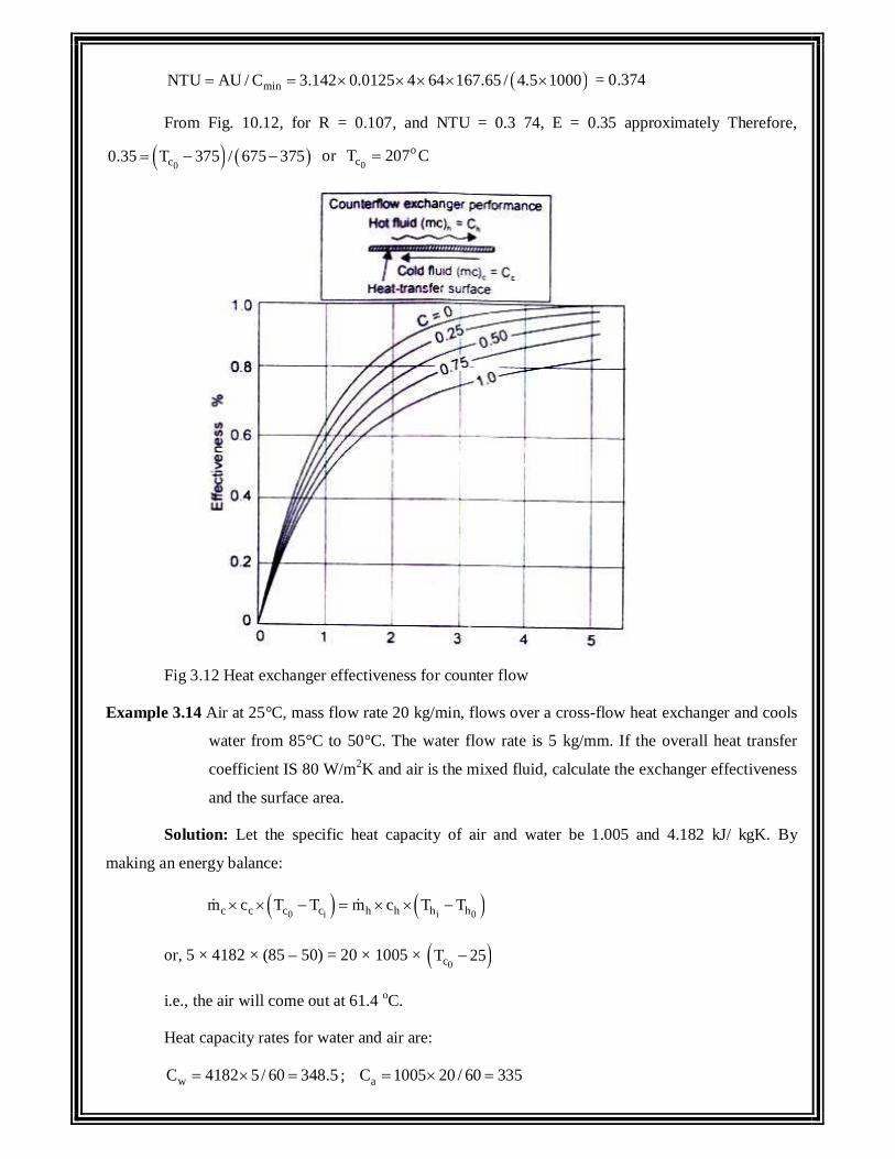
minNTU AU / C 3.142 0.0125 4 64 167.65 / 4.5 1000 = 0.374
From Fig. 10.12, for R = 0.107, and NTU = 0.3 74, E = 0.35 approximately Therefore,
0c0.35 T 375 / 675 375 or 0
ocT 207 C
Fig 3.12 Heat exchanger effectiveness for counter flow
Example 3.14 Air at 25°C, mass flow rate 20 kg/min, flows over a cross-flow heat exchanger and cools
water from 85°C to 50°C. The water flow rate is 5 kg/mm. If the overall heat transfer
coefficient IS 80 W/m2K and air is the mixed fluid, calculate the exchanger effectiveness
and the surface area.
Solution: Let the specific heat capacity of air and water be 1.005 and 4.182 kJ/ kgK. By
making an energy balance:
0 i i 0c c c c h h h hm c T T m c T T
or, 5 × 4182 × (85 – 50) = 20 × 1005 × 0cT 25
i.e., the air will come out at 61.4 oC.
Heat capacity rates for water and air are:
wC 4182 5/ 60 348.5 ; aC 1005 20 / 60 335
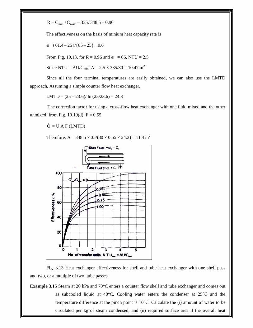
min maxR C / C 335/ 348.5 0.96
The effectiveness on the basis of minium heat capacity rate is
61.4 25 / 85 25 0.6
From Fig. 10.13, for R = 0.96 and = 06, NTU = 2.5
Since NTU = AU/Cmin; A = 2.5 × 335/80 = 10.47 m2
Since all the four terminal temperatures are easily obtained, we can also use the LMTD
approach. Assuming a simple counter flow heat exchanger,
LMTD = (25 – 23.6)/ ln (25/23.6) = 24.3
The correction factor for using a cross-flow heat exchanger with one fluid mixed and the other
unmixed, from Fig. 10.10(d), F = 0.55
Q = U A F (LMTD)
Therefore, A = 348.5 × 35/(80 × 0.55 × 24.3) = 11.4 m2
Fig. 3.13 Heat exchanger effectiveness for shell and tube heat exchanger with one shell pass
and two, or a multiple of two, tube passes
Example 3.15 Steam at 20 kPa and 70°C enters a counter flow shell and tube exchanger and comes out
as subcooled liquid at 40°C. Cooling water enters the condenser at 25°C and the
temperature difference at the pinch point is 10°C. Calculate the (i) amount of water to be
circulated per kg of steam condensed, and (ii) required surface area if the overall heat
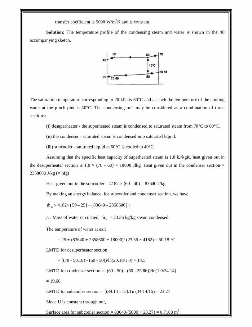
transfer coefficient is 5000 W/m2K and is constant.
Solution: The temperature profile of the condensing steam and water is shown in the 40
accompanying sketch.
The saturation temperature corresponding to 20 kPa is 60°C and as such the temperature of the cooling
water at the pinch pint is 50°C. The condensing unit may be considered as a combination of three
sections:
(i) desuperheater - the superheated steam is condensed to saturated steam from 70°C to 60°C.
(ii) the condenser - saturated steam is condensed into saturated liquid.
(iii) subcooler - saturated liquid at 60°C is cooled to 40°C.
Assuming that the specific heat capacity of superheated steam is 1.8 kJ/kgK, heat given out in
the desuperheater section is 1.8 × (70 - 60) = 18000 Jlkg. Heat given out in the condenser section =
2358600 J/kg (= hfg)
Heat given out in the subcooler = 4182 × (60 - 40) = 83640 J/kg
By making an energy balance, for subcooler and condenser section, we have
wm 4182 50 25 83640 2358600 ;
. Mass of water circulated, wm = 23.36 kg/kg steam condensed.
The temperature of water at exit
= 25 + (83640 + 2358600 + 18000)/ (23.36 × 4182) = 50.18 °C
LMTD for desuperheater section
= [(70 - 50.18) - (60 - 50))/ln(20.18/1 0) = 14.5
LMTD for condenser section = [(60 - 50) - (60 - 25.86))/ln(1 0/34.14)
= 19.66
LMTD for subcooler section = [(34.14 - 15)/1n (34.14/15) = 23.27
Since U is constant through out,
Surface area for subcooler section = 83640/(5000 × 23.27) = 0.7188 m2
Surface area for condenser section = 2358600/(5000 × 19.66) = 23.9939 m2
Surface area for desuperheater section = 18000/(5000 × 14.5) = 0.2483 m2
. Total surface area = 24.96 m2 and average temperature difference = 19.71°C.
Example 3.16 In an economiser (a cross flow heat exchanger, both fluids unmixed) water, mass flow
rate 10 kg/s, enters at 175°C. The flue gas mass flow rate 8 kg/s, specific heat 1.1 kJ/kgK,
enters at 350°C. Estimate the temperature of the flue gas and water at exit, if U = 500
W/m2K, and the surface area 20 m2 What would be the exit temperature if the mass flow
rate of flue gas is (i) doubled, and (ii) halved.
Solution: The heat capacity rate of water = 4182 × 10 = 41820 W /K
The heat capacity rate of flue gas = 1100 × 8 = 8800 W/K
Cmin/Cmax = 8800/41820 = 0.21
minNTU AU / C 500 20 /8800 1.136
From Fig. 10.14. for NTU = 1.136 and min maxC / C 0.21, 0.62
Therefore, 0.62 = (350 - T)/(350 - 175) and T = 241.5°C
The temperature of water at exit, Tw = 175 + 8800 × (350 - 241.5)/41820
= 197.83oC
When the mass flow rate of the flue gas is doubled. Cgas = 17600 W/K
min max minC / C 0.42, NTU AU / C 0.568
= 0.39 = (350 - T)/(350 - 175);
T = 281. 75°C, an increase of 40°C
and Tw = 175 + 28.72 = 203.72°C, an increase of about 6°C.
When the mass flow rate of the flue gas is halved, Cmin = 4400 W/K
min maxC / C 0.105 , NTU = 2.272, and from the figure, = 0.83, an increase and Tg = 204.75
and Tw = 190.3oC
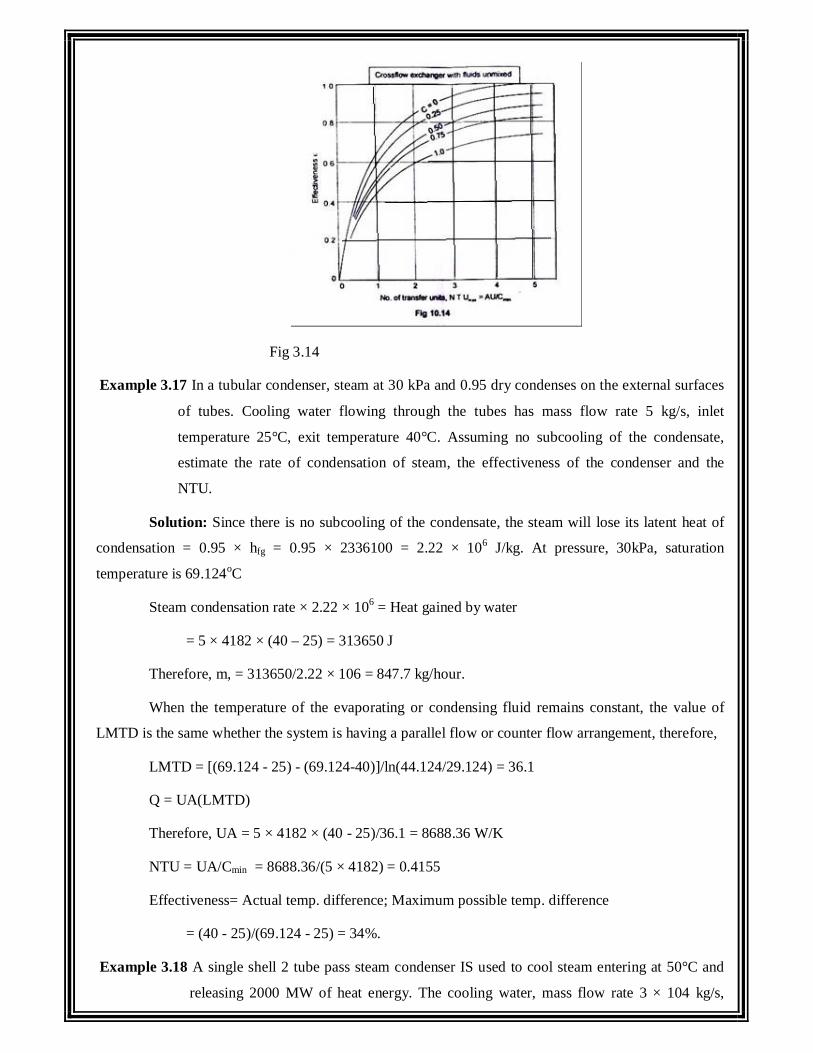
Fig 3.14
Example 3.17 In a tubular condenser, steam at 30 kPa and 0.95 dry condenses on the external surfaces
of tubes. Cooling water flowing through the tubes has mass flow rate 5 kg/s, inlet
temperature 25°C, exit temperature 40°C. Assuming no subcooling of the condensate,
estimate the rate of condensation of steam, the effectiveness of the condenser and the
NTU.
Solution: Since there is no subcooling of the condensate, the steam will lose its latent heat of
condensation = 0.95 × hfg = 0.95 × 2336100 = 2.22 × 10⁶ J/kg. At pressure, 30kPa, saturation
temperature is 69.124oC
Steam condensation rate × 2.22 × 106 = Heat gained by water
= 5 × 4182 × (40 – 25) = 313650 J
Therefore, m, = 313650/2.22 × 106 = 847.7 kg/hour.
When the temperature of the evaporating or condensing fluid remains constant, the value of
LMTD is the same whether the system is having a parallel flow or counter flow arrangement, therefore,
LMTD = [(69.124 - 25) - (69.124-40)]/ln(44.124/29.124) = 36.1
Q = UA(LMTD)
Therefore, UA = 5 × 4182 × (40 - 25)/36.1 = 8688.36 W/K
NTU = UA/Cmin = 8688.36/(5 × 4182) = 0.4155
Effectiveness= Actual temp. difference; Maximum possible temp. difference
= (40 - 25)/(69.124 - 25) = 34%.
Example 3.18 A single shell 2 tube pass steam condenser IS used to cool steam entering at 50°C and
releasing 2000 MW of heat energy. The cooling water, mass flow rate 3 × 10⁴ kg/s,
enters the condenser at 25°C. The condenser has 30,000 thin walled tube of 30 mm
diameter. If the overall heat transfer coefficient is 4000 Wim2K, estimate the (I) rise m
temperature of the cooling water, and (II) length of the tube per pass.
Solution: By making an energy balance:
Heat released by steam = heat taken in by cooling water,
or, 2000 × 106 = 3 × 104 × 4182 × ( T); T = 15.94°C.
Since in a condenser, heat capacity rate of condensing steam is usually very large m
comparison with the heat capacity rate of cooling water, the effectiveness
0 i i ic c h cT T / T T 15.94 / 50 25 0.6376
And, for min maxC / C 0, 1 exp NTU
exp NTU 1.0 0.6376 0.3624
And, minNTU 1.015 AU / C 2 3.142 0.03 L 30000 4000 / 1.25 108
L = 5.546 m
3.10. Heat Exchanger Design-Important Factors
A comprehensive design of a heat exchanger involves the consideration of the thermal,
mechanical and manufacturing aspect. The choice of a particular design for a given duty depends on
either the selection of an existing design or the development of a new design. Before selecting an
existing design, the analysis of his performance must be made to see whether the required performance
would be obtained within acceptable limits.
In the development of a new design, the following factors are important:
(a) Fluid Temperature - the temperature of the two fluid streams are either specified for a given
inlet temperature, or the designer has to fix the outlet temperature based on flow rates and heat transfer
considerations. Once the terminal temperatures are defined, the effectiveness of the heat exchanger
would give an indication of the type of flow path-parallel or counter or cross-flow.
(b) Flow Rates - The maximum velocity (without causing excessive pressure drops, erosion,
noise and vibration, etc.) in the case of liquids is restricted to 8 m1s and m case of gases below 30 m/s.
With this restriction, the flow rates of the two fluid streams lead to the selection of flow passage cross-
sectional area required for each of the two fluid steams.
(c) Tube Sizes and Layout - Tube sizes, thickness, lengths and pitches have strong influence on
heat transfer calculations and therefore, these are chosen with great care. The sizes of tubes vary from
1/4" O.D. to 2" O.D.; the more commonly used sizes are: 5/8", 3/4" and 1" O.D. The sizes have to be
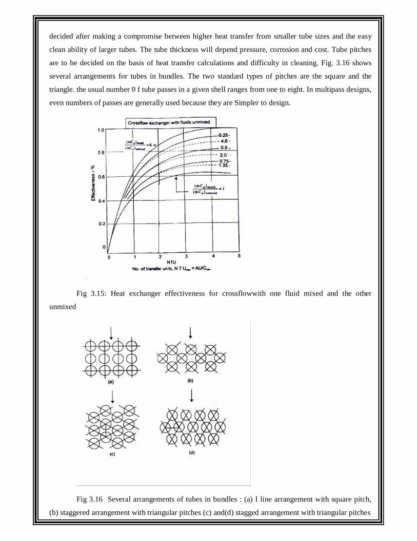
decided after making a compromise between higher heat transfer from smaller tube sizes and the easy
clean ability of larger tubes. The tube thickness will depend pressure, corrosion and cost. Tube pitches
are to be decided on the basis of heat transfer calculations and difficulty in cleaning. Fig. 3.16 shows
several arrangements for tubes in bundles. The two standard types of pitches are the square and the
triangle. the usual number 0 f tube passes in a given shell ranges from one to eight. In multipass designs,
even numbers of passes are generally used because they are Simpler to design.
Fig 3.15: Heat exchanger effectiveness for crossflowwith one fluid mixed and the other
unmixed
Fig 3.16 Several arrangements of tubes in bundles : (a) I line arrangement with square pitch,
(b) staggered arrangement with triangular pitches (c) and(d) stagged arrangement with triangular pitches
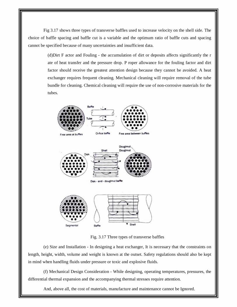
Fig 3.17 shows three types of transverse baffles used to increase velocity on the shell side. The
choice of baffle spacing and baffle cut is a variable and the optimum ratio of baffle cuts and spacing
cannot be specified because of many uncertainties and insufficient data.
(d)Dirt F actor and Fouling - the accumulation of dirt or deposits affects significantly the r
ate of heat transfer and the pressure drop. P roper allowance for the fouling factor and dirt
factor should receive the greatest attention design because they cannot be avoided. A heat
exchanger requires frequent cleaning. Mechanical cleaning will require removal of the tube
bundle for cleaning. Chemical cleaning will require the use of non-corrosive materials for the
tubes.
Fig. 3.17 Three types of transverse baffles
(e) Size and Installation - In designing a heat exchanger, It is necessary that the constraints on
length, height, width, volume and weight is known at the outset. Safety regulations should also be kept
in mind when handling fluids under pressure or toxic and explosive fluids.
(f) Mechanical Design Consideration - While designing, operating temperatures, pressures, the
differential thermal expansion and the accompanying thermal stresses require attention.
And, above all, the cost of materials, manufacture and maintenance cannot be Ignored.
Example 3.19 In a counter flow concentric tube heat exchanger cooling water, mass flow rate 0.2 kg/s,
enters at 30°C through a tube inner diameter 25rnnl. The oil flowing through the
annulus, mass flow rate 0.1 kg/s, diameter 45 rum, has temperature at inlet 100°C.
Calculate the length of the tube if the oil comes out at 60°C. The properties of oil and
water are:
Oil: Cp – 2131 J/kgK, = 3.25 × 10⁻² Pa-s, k = 0.138 W/mK,
Water; Cp = 4178 J/kg K, = 725 × 10–6 Pa-s,
k = 0.625 W/mK, Pr = 4.85
Solution: By making an energy balance: Heat given out by oil = heat taken in by water.
0c0.1 2131 100 60 0.2 4187 T 30
0o
cT 40.2 C
LMTD = i 0 0 i i 0 0 0h c h c h c h cT T T T / ln T T / T T
o100 40.2 60 30 / ln 59.8 / 30 43.2 C
Since water is flowing through the tube,
64 0.2Re 4m / D
3.142 0.025 725 10
= 14050, a turbulent flow.
Nu = 0.023 Re0.8 Pr0.4, fluid being heated.
= 0.023 (14050)0.8 (4.85)0.4 = 90; ih = 90 × 0.625/0.025 = 2250 W/m2K
The oil is flowing through the annulus for which the hydraulic diameter is:
(0.045 - 0.025) = 0.02 m
2o iRe 4m / D D 4 0.1/ 3.142 0.07 3.25 10 56.0
laminar flow.
Assuming Uniform temperature along the Inner surface of the annulus and a perfectly insulated
outer surface.
Nu = 5.6, by interpolation (chapter 6)
ho = 5.6 × 0.138/0.02 = 38.6 W/m2K.
The overall heat transfer coefficient after neglecting the tube wall resistance,
U = 1/(1/2250 + 1/38.6) = 38 W/m2K
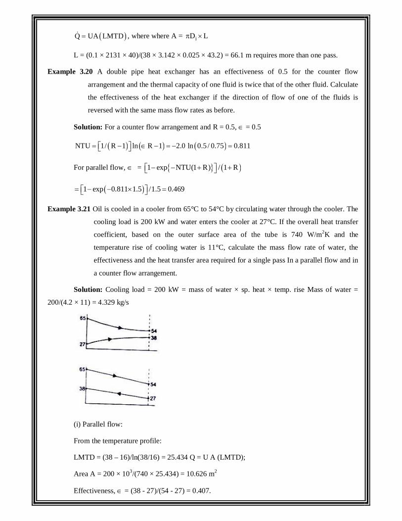
Q UA LMTD , where where A = iD L
L = (0.1 × 2131 × 40)/(38 × 3.142 × 0.025 × 43.2) = 66.1 m requires more than one pass.
Example 3.20 A double pipe heat exchanger has an effectiveness of 0.5 for the counter flow
arrangement and the thermal capacity of one fluid is twice that of the other fluid. Calculate
the effectiveness of the heat exchanger if the direction of flow of one of the fluids is
reversed with the same mass flow rates as before.
Solution: For a counter flow arrangement and R = 0.5, = 0.5
NTU 1/ R 1 ln R 1 2.0 ln 0.5 / 0.75 0.811
For parallel flow, = 1 exp NTU(1 R) / 1 R
1 exp 0.811 1.5 /1.5 0.469
Example 3.21 Oil is cooled in a cooler from 65°C to 54°C by circulating water through the cooler. The
cooling load is 200 kW and water enters the cooler at 27°C. If the overall heat transfer
coefficient, based on the outer surface area of the tube is 740 W/m2K and the
temperature rise of cooling water is 11°C, calculate the mass flow rate of water, the
effectiveness and the heat transfer area required for a single pass In a parallel flow and in
a counter flow arrangement.
Solution: Cooling load = 200 kW = mass of water × sp. heat × temp. rise Mass of water =
200/(4.2 × 11) = 4.329 kg/s
(i) Parallel flow:
From the temperature profile:
LMTD = (38 – 16)/ln(38/16) = 25.434 Q = U A (LMTD);
Area A = 200 × 103/(740 × 25.434) = 10.626 m2
Effectiveness, = (38 - 27)/(54 - 27) = 0.407.
(ii) Counter flow:
From the temperature profile:
LMTD = mean temperature difference = 27°C
Area A = 200 × 103/(740 × 27) = 10 m2
Effectiveness, E = (38 - 27)/(65 - 27) = 0.289.
Example 3.22 Oil (mass flow rate 1.5 kg/s Cp = 2 kJ/kgK) is cooled in a single pass shell and tube
heat exchanger from 65 to 42°C. Water (mass flow rate 1 kg/s, Cp = 4.2 kJ/kgK) has
an inlet temperature of 28°C. If the overall heat transfer coefficient is 700 W/m2K,
calculate heat transfer area for a counter flow arrangement using - NTU method.
Solution: Heat capacity rate of 011; 1.5 × 2.0 = 3 kW/K
Heat capacity rate of water = 1 × 4.2; 4.2 kW/K
minC 3.0 kW / K and min maxR C / C 3/ 4.2 0.714
For a counter flow arrangement, NTU 1/ R 1 ln 1 / R 1
Effectiveness, 65 42 / 65 28 0.6216
and NTU = 1.346 = minA U / C ; A = 1.346 × 3000 / 700 = 5.77 m2
By making an energy balance, we can compute the water temperature at outlet.
or 3.0 × (65 - 42); 4.2 × (T - 28), T; 44.428
LMTD for a counter flow arrangement:
LMTD; (20.572 - 14)/ln (20.572/14) = 17.076
Area, A = 3 2Q / U LMTD 3 10 65 42 / 700 17.076 5.77 m
Example 3.23 A fluid (mass flow rate 1000 kg/min, sp. heat capacity 3.6 kJ/kgK) enters a heat
exchanger at 700 C. Another fluid (mass flow rate 1200 kg/mm, sp. heal capacity 4.2
kJ/kgK) enters al 100 C. If the overall heat transfer coefficient is 420 W/m2K and the
surface area is 100m2, calculate the outlet temperatures of both fluids for both counter
flow and parallel flow arrangements.
Solution: Heat capacity rate for the hot fluid
3 31000 3.6 10 60 60 10 W / K
Heat capacity rate for the cold fluid = 1200 × 4.2 × 103/60 = 84 × 103 W/K
R = Cmin/Cmax = 60/84; 0.714, NTU = U A/Cmin = 420 × 100/60000 = 0.7
(i) For counter flow heat exchanger:
1 exp N 1 R / 1 Re xp N 1 R
1 exp 0.7 1 0.714 /1 1 0.714 exp 0.7 1 0.714 0.4367
Since heat capacity rate of the hot fluid IS lower,
0h700 T / 700 100
and 0
ohT 700 0.4367 600 438 C
By making an energy balance, 03 3
c60 10 700 438 84 10 T 100
or, 0
ocT 60 262 /84 100 87.14 C
(ii) For parallel flow heat exchanger
1 exp N 1 R / 1 R 1 exp 0.7 1 0.714 / 1.714
0.4077 , a lower value
and i 0 i 0 0 0h h h c h cT T / T T 0.4077 700 T / 700 T
By making an energy balance: 0 03 3
h c60 10 700 T 84 10 T 100
or, 0 0c h700 T 700 T / 0.4077
and 0 0c c84 T 100 / 60 1.4T 140
Therefore, 0
ocT 237.5 C
and 0
ohT 511.4 C
Example 3.24 Steam enters the surface condenser at 100°C and water enters at 25°C with a temperature
rise of 25°C. Calculate the effectiveness and the NTU for the condenser. If the water
temperature at inlet changes to 35 C, estimate the temperature rise for water.
Solution: Effectiveness, = 25/(100 25) = 0.33
For R = 0, = 1 - exp(- N)
or, N = -ln(1 - ) = 0.405
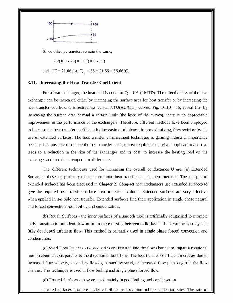
Since other parameters remain the same,
25/(100 - 25) = T/(100 - 35)
and T = 21.66; or, 0cT = 35 + 21.66 = 56.66°C.
3.11. Increasing the Heat Transfer Coefficient
For a heat exchanger, the heat load is equal to Q = UA (LMTD). The effectiveness of the heat
exchanger can be increased either by increasing the surface area for heat transfer or by increasing the
heat transfer coefficient. Effectiveness versus NTU(AU/Cmin) curves, Fig. 10.10 - 15, reveal that by
increasing the surface area beyond a certain limit (the knee of the curves), there is no appreciable
improvement in the performance of the exchangers. Therefore, different methods have been employed
to increase the heat transfer coefficient by increasing turbulence, improved mixing, flow swirl or by the
use of extended surfaces. The heat transfer enhancement techniques is gaining industrial importance
because it is possible to reduce the heat transfer surface area required for a given application and that
leads to a reduction in the size of the exchanger and its cost, to increase the heating load on the
exchanger and to reduce temperature differences.
The 'different techniques used for increasing the overall conductance U are: (a) Extended
Surfaces - these are probably the most common heat transfer enhancement methods. The analysis of
extended surfaces has been discussed in Chapter 2. Compact heat exchangers use extended surfaces to
give the required heat transfer surface area in a small volume. Extended surfaces are very effective
when applied in gas side heat transfer. Extended surfaces find their application in single phase natural
and forced convection pool boiling and condensation.
(b) Rough Surfaces - the inner surfaces of a smooth tube is artificially roughened to promote
early transition to turbulent flow or to promote mixing between bulk flow and the various sub-layer in
fully developed turbulent flow. This method is primarily used in single phase forced convection and
condensation.
(c) Swirl Flow Devices - twisted strips are inserted into the flow channel to impart a rotational
motion about an axis parallel to the direction of bulk flow. The heat transfer coefficient increases due to
increased flow velocity, secondary flows generated by swirl, or increased flow path length in the flow
channel. This technique is used in flow boiling and single phase forced flow.
(d) Treated Surfaces - these are used mainly in pool boiling and condensation.
Treated surfaces promote nucleate boiling by providing bubble nucleation sites. The rate of
condensation increases by promoting the formation of droplets, instead of a liquid film on the
condensing surface. This can be accomplished by coating the surface with a material that makes the
surface non-wetting.
All of these techniques lead to an increase in pumping work (increased frictional losses) and
any practical application requires the economic benefit of increased overall conductance. That is, a
complete analysis should be made to determine the increased first cost because of these techniques,
increased heat exchanger heat transfer performance, the effect on operating costs (especially a
substantial increase in pumping power) and maintenance costs.
3.12. Fin Efficiency and Fin Effectiveness
Fins or extended surfaces increase the heat transfer area and consequently, the amount of heat
transfer is increased. The temperature at the root or base of the fin is the highest and the temperature
along the length of the fm goes on decreasing Thus, the fin would dissipate the maximum amount of
heat energy if the temperature all along the length remains equal to the temperature at the root. Thus, the
fin efficiency is defined as:
fin = (actual heat transferred) / (heat which would be transferred if the entire fin area were at
the root temperature)
In some cases, the performance of the extended surfaces is evaluated by comparing the heat
transferred with the fin to the heat transferred without the fin. This ratio is called 'fin effectiveness' E
and it should be greater than 1, if the rate of heat transfer has to be increased with the use of fins.
For a very long fin, effectiveness E = Q with fin / Q without fin
= (hpkA)1/ 20 /hA 0 = (kp/hA)1/2
And fin = (hpkA) 1/ 20 (hpL 0 ) = (hpkA)1/2 / (hpL)
1/ 2
1/ 2fin
kp / hAE pL Surface area of finhpLA Cross-sectional area of the finhpkA
i.e., effectiveness increases by increasing the length of the fin but it will decrease the fin
efficiency.
Expressions for Fin Efficiency for Fins of Uniform Cross-section
1. Very long fins: 1/ 20 0hpkA T T / hpL T T 1/ mL
2 For fins having insulated tips:
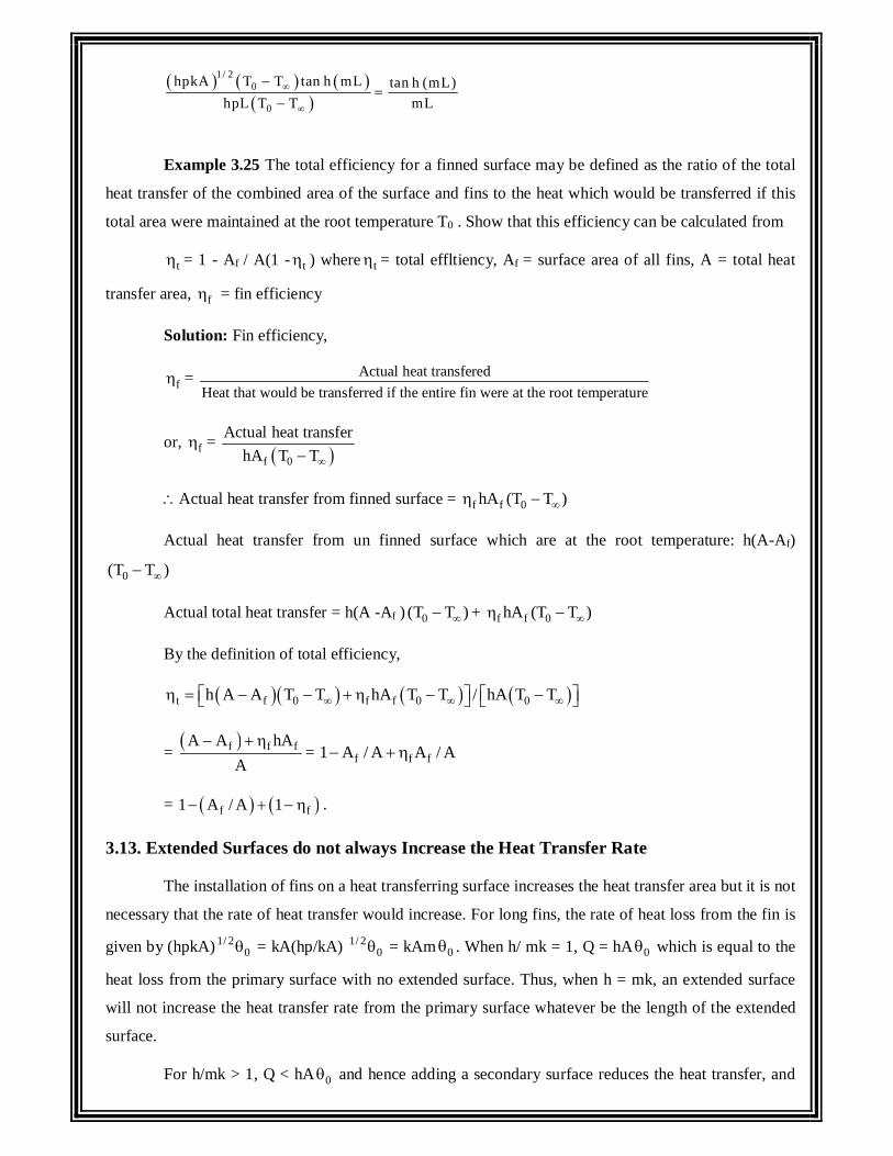
1 / 20
0
hpkA T T tan h mL tan h (mL)hpL T T mL
Example 3.25 The total efficiency for a finned surface may be defined as the ratio of the total
heat transfer of the combined area of the surface and fins to the heat which would be transferred if this
total area were maintained at the root temperature T0 . Show that this efficiency can be calculated from
t = 1 - Af / A(1 - t ) where t = total effltiency, Af = surface area of all fins, A = total heat
transfer area, f = fin efficiency
Solution: Fin efficiency,
f = Actual heat transferedHeat that would be transferred if the entire fin were at the root temperature
or, f = f 0
Actual heat transferhA T T
Actual heat transfer from finned surface = f f 0hA (T T )
Actual heat transfer from un finned surface which are at the root temperature: h(A-Af)
0(T T )
Actual total heat transfer = h(A -Af ) 0(T T ) + f f 0hA (T T )
By the definition of total efficiency,
t f 0 f f 0 0h A A T T hA T T / hA T T
= f f fA A hA
A
= f f f1 A / A A / A
= f f1 A / A 1 .
3.13. Extended Surfaces do not always Increase the Heat Transfer Rate
The installation of fins on a heat transferring surface increases the heat transfer area but it is not
necessary that the rate of heat transfer would increase. For long fins, the rate of heat loss from the fin is
given by (hpkA) 1/ 20 = kA(hp/kA) 1/ 2
0 = kAm 0 . When h/ mk = 1, Q = hA 0 which is equal to the
heat loss from the primary surface with no extended surface. Thus, when h = mk, an extended surface
will not increase the heat transfer rate from the primary surface whatever be the length of the extended
surface.
For h/mk > 1, Q < hA 0 and hence adding a secondary surface reduces the heat transfer, and
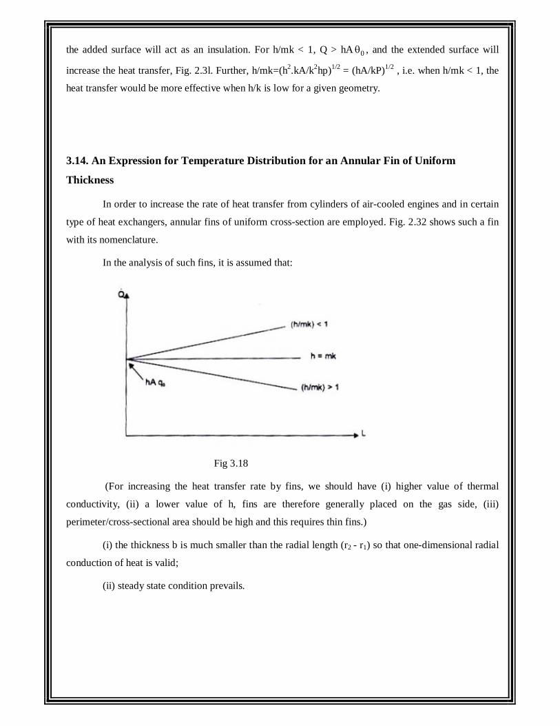
the added surface will act as an insulation. For h/mk < 1, Q > hA 0 , and the extended surface will
increase the heat transfer, Fig. 2.3l. Further, h/mk=(h2.kA/k2hp)1/2 = (hA/kP)1/2 , i.e. when h/mk < 1, the
heat transfer would be more effective when h/k is low for a given geometry.
3.14. An Expression for Temperature Distribution for an Annular Fin of Uniform
Thickness
In order to increase the rate of heat transfer from cylinders of air-cooled engines and in certain
type of heat exchangers, annular fins of uniform cross-section are employed. Fig. 2.32 shows such a fin
with its nomenclature.
In the analysis of such fins, it is assumed that:
Fig 3.18
(For increasing the heat transfer rate by fins, we should have (i) higher value of thermal
conductivity, (ii) a lower value of h, fins are therefore generally placed on the gas side, (iii)
perimeter/cross-sectional area should be high and this requires thin fins.)
(i) the thickness b is much smaller than the radial length (r2 - r1) so that one-dimensional radial
conduction of heat is valid;
(ii) steady state condition prevails.
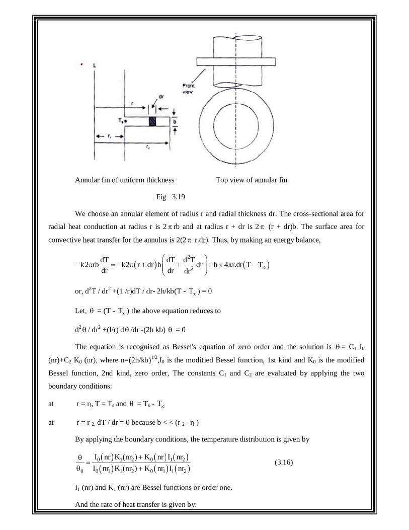
Annular fin of uniform thickness Top view of annular fin
Fig 3.19
We choose an annular element of radius r and radial thickness dr. The cross-sectional area for
radial heat conduction at radius r is 2 rb and at radius r + dr is 2 (r + dr)b. The surface area for
convective heat transfer for the annulus is 2(2 r.dr). Thus, by making an energy balance,
2
2dT dT d Tk2 rb k2 r dr b dr h 4 r.dr T Tdr dr dr
or, d2T / dr2 +(1 /r)dT / dr- 2h/kb(T - T ) = 0
Let, = (T - T ) the above equation reduces to
d2 / dr2 +(l/r) d /dr -(2h kb) = 0
The equation is recognised as Bessel's equation of zero order and the solution is = C1 I0
(nr)+C2 K0 (nr), where n=(2h/kb)1/2,I0 is the modified Bessel function, 1st kind and K0 is the modified
Bessel function, 2nd kind, zero order, The constants C1 and C2 are evaluated by applying the two
boundary conditions:
at r = rl, T = Ts and = Ts - T
at r = r 2, dT / dr = 0 because b < < (r 2 - rl )
By applying the boundary conditions, the temperature distribution is given by
0 1 2 0 1 2
0 0 1 1 2 0 1 1 2
I nr K (nr ) K nr I nrI nr K (nr ) K nr I nr
(3.16)
I1 (nr) and K1 (nr) are Bessel functions or order one.
And the rate of heat transfer is given by:
1 1 1 2 1 1 1 20 1
0 1 1 2 0 1 1 2
K nr I (nr ) I nr K nrQ 2 knb r
K nr I (nr ) I nr K nr
(3.17)
Table 2.1 gives selected values of the Modified Bessel Functions of the First and Second kinds,
order Zero and One. (The details of solution can be obtained from: C.R. Wylie, Jr: Advanced
Engineering Mathematics, McGraw-Hill Book Company, New York.)
The efficiency of circumferential fins is also obtained from curves for efficiencies
3 12 2
2 1 2 1b 2halong Y-axis r r r r2 Kb
for different values of 2 1br / r2
.