course 395: machine learning - lectures · stavros petridis machine learning (course 395) course...

Stavros Petridis Machine Learning (course 395)

Course 395: Machine Learning - Lectures • Lecture 1-2: Concept Learning (M. Pantic)

•Lecture 3-4: Decision Trees & CBC Intro (M. Pantic & S. Petridis)

•Lecture 5-6: Evaluating Hypotheses (S. Petridis)

•Lecture 7-8: Artificial Neural Networks I (S. Petridis)

•Lecture 9-10: Artificial Neural Networks II (S. Petridis)

•Lecture 11-12: Instance Based Learning (M. Pantic)

•Lecture 13-14: Genetic Algorithms (M. Pantic)


Evaluating Hypotheses – Lecture Overview

• Measures of classification performance – Classification Error Rate

– UAR

– Recall, Precision, Confusion Matrix

– Imbalanced Datasets

– Overfitting

– Cross-validation

• Estimating hypothesis accuracy – Sample Error vs. True Error

– Confidence Intervals

– Binomial and Normal Distributions

• Comparing Learning Algorithms – t-test


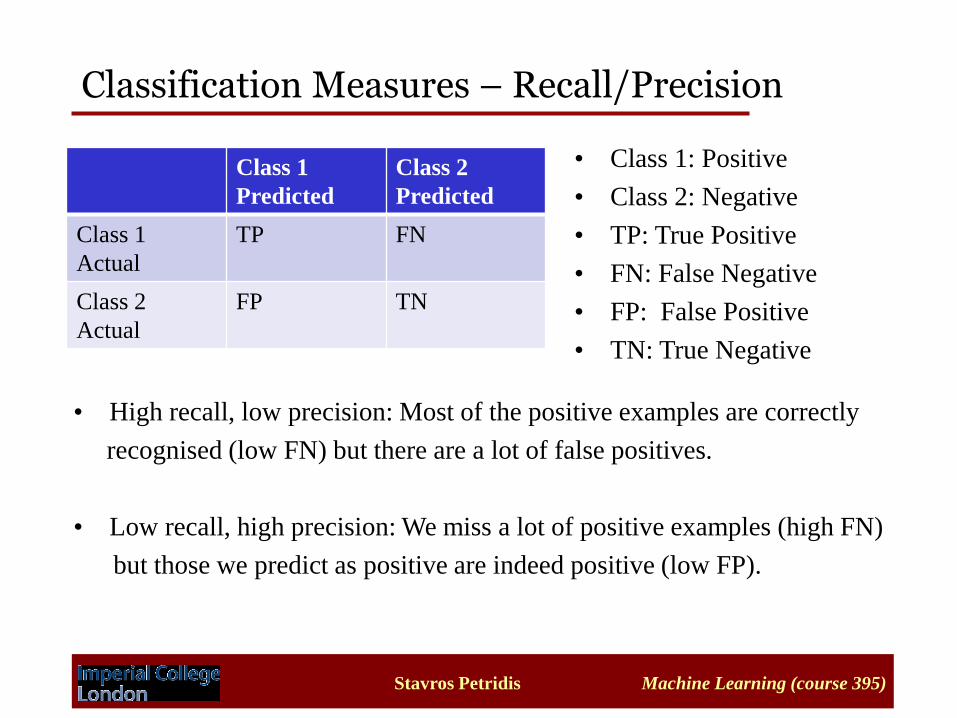
Classification Measures – Confusion Matrix

Class 1

Predicted

Class 2

Predicted

Class 1

Actual

TP FN

Class 2

Actual

FP TN

• Class 1: Positive

• Class 2: Negative

• TP: True Positive

• FN: False Negative

• FP: False Positive

• TN: True Negative

• Visualisation of the performance of an algorithm

• Allows easy identification of confusion between between classes

e.g. one class is commonly mislabelled as the other

• Most performance measures are computed from the confusion matrix


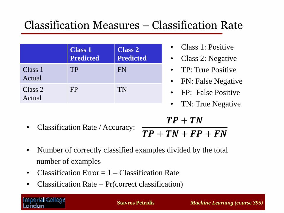
Classification Measures – Classification Rate

Class 1

Predicted

Class 2

Predicted

Class 1

Actual

TP FN

Class 2

Actual

FP TN







• Classification Rate / Accuracy:

• Number of correctly classified examples divided by the total

number of examples

• Classification Error = 1 – Classification Rate

• Classification Rate = Pr(correct classification)


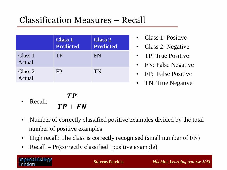
Classification Measures – Recall

Class 1

Predicted

Class 2

Predicted

Class 1

Actual

TP FN

Class 2

Actual

FP TN







• Recall:

• Number of correctly classified positive examples divided by the total

number of positive examples

• High recall: The class is correctly recognised (small number of FN)

• Recall = Pr(correctly classified | positive example)


Classification Measures – Precision

Class 1

Predicted

Class 2

Predicted

Class 1

Actual

TP FN

Class 2

Actual

FP TN







• Precision:

• Number of correctly classified positive examples divided by the total

number of predicted positive examples

• High precision: An example labeled as positive is indeed positive

(small number of FP)

• Precision = Pr(positive example | example is classified as positive)

𝑻𝑷

𝑻𝑷 + 𝑭𝑷


Classification Measures – Recall/Precision

Class 1

Predicted

Class 2

Predicted

Class 1

Actual

TP FN

Class 2

Actual

FP TN







• High recall, low precision: Most of the positive examples are correctly

recognised (low FN) but there are a lot of false positives.

• Low recall, high precision: We miss a lot of positive examples (high FN)

but those we predict as positive are indeed positive (low FP).


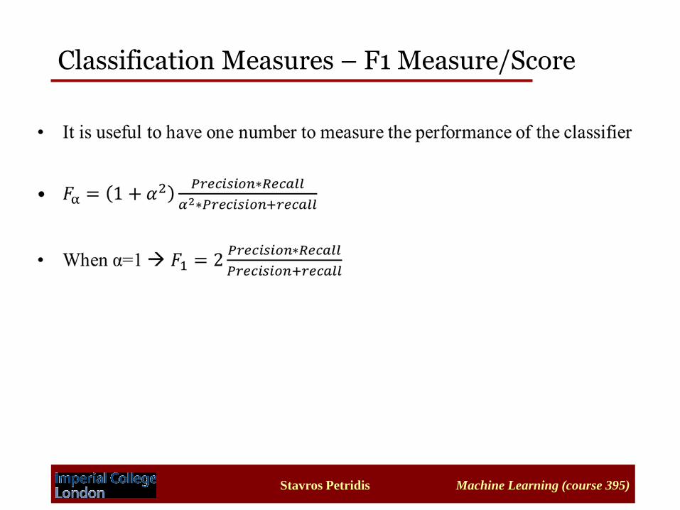
Classification Measures – F1 Measure/Score


Classification Measures – UAR

Class 1

Predicted

Class 2

Predicted

Class 1

Actual

TP FN

Class 2

Actual

FP TN







• We compute recall for class1 (R1) and for class2 (R2).

• Unweighted Average Recall (UAR) = mean(R1, R2)


Classification Measures – Extension to Multiple Classes

Class 1

Predicted

Class 2

Predicted

Class 3

Predicted

Class 1

Actual

TP FN FN

Class 2

Actual

FP TN

?

Class 3

Actual

FP ? TN

• In the multiclass case it is still

very useful to compute the

confusion matrix.

• We can define one class as

positive and the other as negative.

• We can compute the performance

measures in exactly the same way.

• CR = number of correctly classified examples (trace) divided by the

total number of examples.

• Recall and precision and F1 are still computed for each class.

• UAR = mean(R1, R2, R3,…, RN)


Classification Measures – Balanced Dataset

Class 1

Predicted

Class 2

Predicted

Class 1

Actual

70 30

Class 2

Actual

10 90

• CR: 80%

• Recall (cl.1): 70%

• Precision (cl.1): 87.5%

• F1 (cl.1): 77.8%

• UAR: 80%


• Precision (cl.2): 75%

• F1 (cl.2): 81.8%

• Balanced Dataset: The number of examples in each class

are similar

• All measures result in similar performance


Classification Measures – Imbalanced Dataset Case 1: Both classifiers are good

Class 1

Predicted

Class 2

Predicted

Class 1

Actual

700 300

Class 2

Actual

10 90

• CR: 71.8%



• F1 (cl.1): 81.9%

• UAR: 80%



• F1 (cl.2): 36.8%

• Imbalanced Dataset: Classes are not equally represented

• CR goes down, is affected a lot by the majority class

• Precision (and F1) for Class 2 is significantly affected –

- 30% of class1 examples are misclassified leads to a

higher number of FP than TN due to imbalance


Classification Measures – Imbalanced Dataset Case 2: One classifier is useless

Class 1

Predicted

Class 2

Predicted

Class 1

Actual

700 300

Class 2

Actual

100 0

• CR: 70%



• F1 (cl.1): 77.8%

• UAR: 35%



• F1 (cl.2): Not defined

• CR is misleading, one classifier is useless.

• F1 for class2 and UAR tell us that something is wrong.

• UAR also detects that there is a problem.


Classification Measures – Imbalanced Dataset Conclusions

• CR can be misleading, simply follows the performance of the

majority class

• UAR is useful and can help to detect that one or more classifiers are

not good but it does not give us any information about FP

• F1 is useful as well but is also affected by the class imbalance

problem

- We are not sure if the low score is due to one/more classifiers being

useless or class imbalance

• That’s why we should always have a look at the confusion matrix


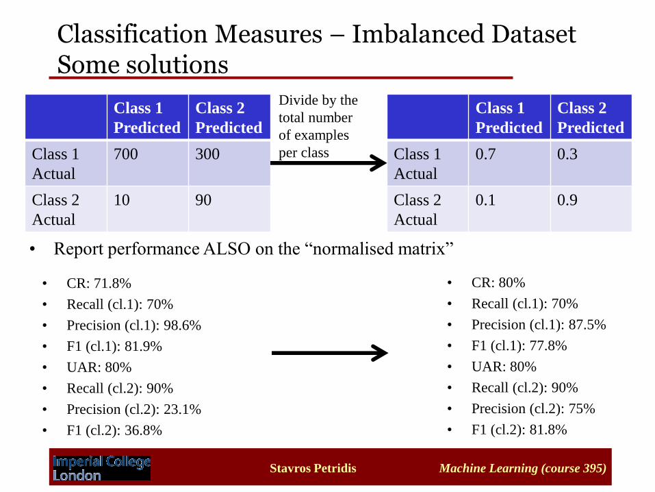
Classification Measures – Imbalanced Dataset Some solutions

• Report performance ALSO on the “normalised matrix”

Class 1

Predicted

Class 2

Predicted

Class 1

Actual

700 300

Class 2

Actual

10 90

Class 1

Predicted

Class 2

Predicted

Class 1

Actual

0.7 0.3

Class 2

Actual

0.1 0.9

Divide by the

total number

of examples

per class

• CR: 71.8%



• F1 (cl.1): 81.9%

• UAR: 80%



• F1 (cl.2): 36.8%

• CR: 80%



• F1 (cl.1): 77.8%

• UAR: 80%



• F1 (cl.2): 81.8%


Classification Measures – Imbalanced Dataset Some solutions

• Upsample the minority class

• Downsample the majority class

- e.g. select randomly the same number of examples as the minority class.

- Repeat this procedure several times and train a classifier each time

with a different training set.

- Report the mean and st. dev. of the selected performance measure

• Japkowicz, Nathalie, and Shaju Stephen. "The class imbalance problem:

A systematic study." Intelligent data analysis 6.5 (2002): 429-449.


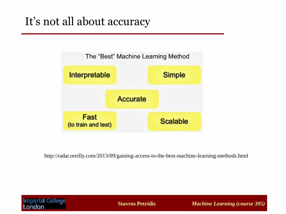
It’s not all about accuracy

http://radar.oreilly.com/2013/09/gaining-access-to-the-best-machine-learning-methods.html


https://www.techdirt.com/blog/innovation/articles/20120409/03412518422/


Training/Validation/Test Sets

• Split your dataset into 3 disjoint sets: Training, Validation, Test

• If a lot of data are available then you can try 50:25:25 otherwise

60:20:20.

• Identify which parameters need to be optimised and select a performance

measure to evaluate the performance on the validation set.

- e.g. number of hidden neurons

- Use F1 as performance measure. It’s perfectly fine to use any other measure,

depends on your application


• Train your algorithm on the training set multiple times, each time

using different values for the parameters you wish to optimise.

• For each trained classifier evaluate the performance on the

validation set (using the performance measure you have selected).



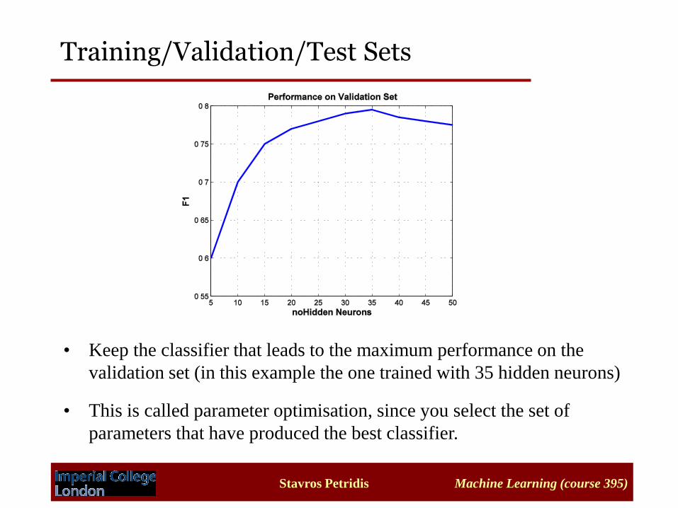
• Keep the classifier that leads to the maximum performance on the

validation set (in this example the one trained with 35 hidden neurons)

• This is called parameter optimisation, since you select the set of

parameters that have produced the best classifier.




• Test the performance on the test set.

• The test set should NOT be used for training or validation. It is used

ONLY in the end for estimating the performance on unknown examples,

i.e. how well your trained classifiers generalises.

• You should assume that you do not know the labels of the test set and

only after you have trained your classifier they are given to you.


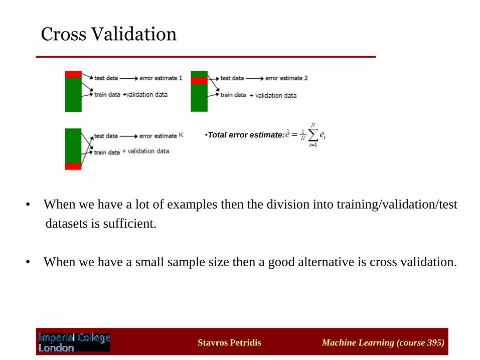
Cross Validation

• When we have a lot of examples then the division into training/validation/test

datasets is sufficient.

• When we have a small sample size then a good alternative is cross validation.

•Total error estimate:


Cross Validation – Parameter Optimisation + Test Set Performance

• Divide dataset into k (usually 10) folds using k-1 for training+validation

and one for testing

• Test data between different folds should never overlap!

• Training+Validation and test data in the same iteration should never overlap!

• In each iteration the error on the left-out test set is estimated

• Error estimate: average of the k errors

•Total error estimate:



• We can run an n (usually 2-3) fold cross-validation on the training+validation

folds only in order to optimise the parameters.

• Select the parameters that result in the best average performance over all n folds.

• Then train on the entire training+validation set (k-1 folds) and test on the k fold.

• Inner cross-validation: Parameter Optimisation

• Outer cross-validation: Performance evaluation

Test data

n-fold cross validation

on k-1 folds only

Validation data

Training

data

k-1

folds

Validation data

Training

data … Repeat k times



• Another simpler way to optimise the parameters is simply to leave a second

fold out for validation.

• Train on the training set, optimise parameters on the validation set and test

on the test set.

S. Marsland, Machine learning: An algorithmic perspective


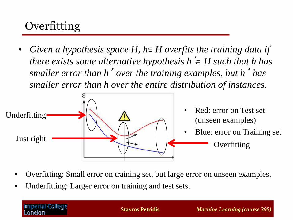
Overfitting

• Given a hypothesis space H, h H overfits the training data if

there exists some alternative hypothesis h’ H such that h has

smaller error than h’ over the training examples, but h’ has

smaller error than h over the entire distribution of instances.

• Red: error on Test set

(unseen examples)

• Blue: error on Training set

• Overfitting: Small error on training set, but large error on unseen examples.

• Underfitting: Larger error on training and test sets.

Underfitting

Overfitting Just right


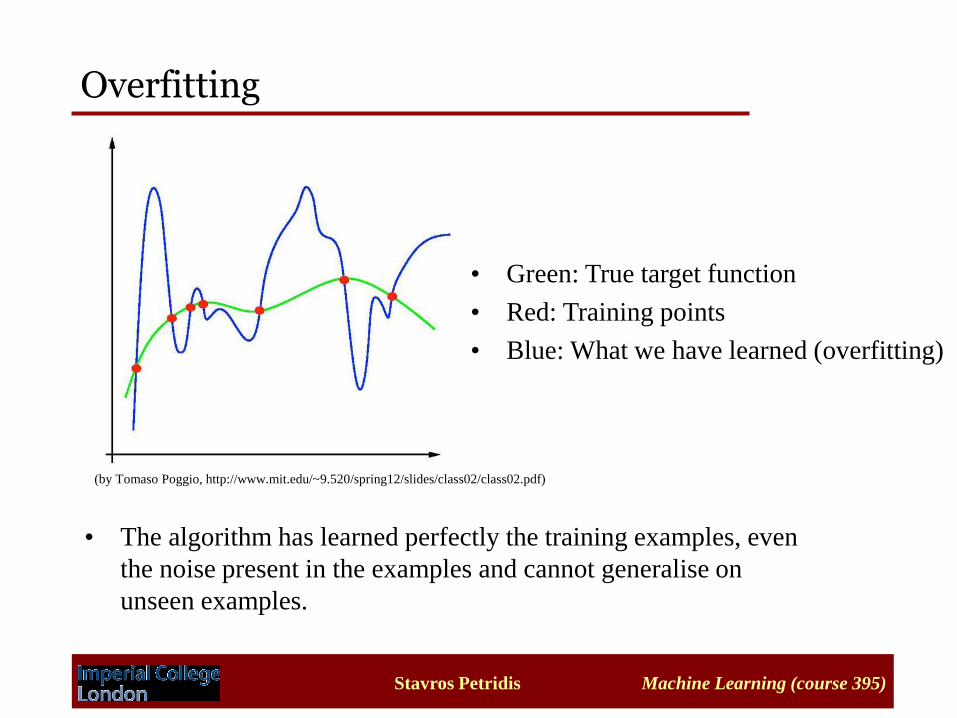
Overfitting

• The algorithm has learned perfectly the training examples, even

the noise present in the examples and cannot generalise on

unseen examples.

• Green: True target function

• Red: Training points

• Blue: What we have learned (overfitting)

(by Tomaso Poggio, http://www.mit.edu/~9.520/spring12/slides/class02/class02.pdf)


Overfitting

• Overfitting can occur when:

– Learning is performed for too long (e.g. in Neural Networks).

– The examples in the training set are not representative of all

possible situations.

– The model we use is too complex.

http://www.astroml.org/sklearn_tutorial/practical.html


Estimating accuracy of classification measures

• Q1: What is the best estimate of the accuracy over future examples

drawn from the same distribution?

- If future examples are drawn from a different distribution then we

cannot generalise our conclusions based on the sample we already

have.

• Q2: What is the probable error in this accuracy estimate? We want to

assess the confidence that we can have in this classification measure.


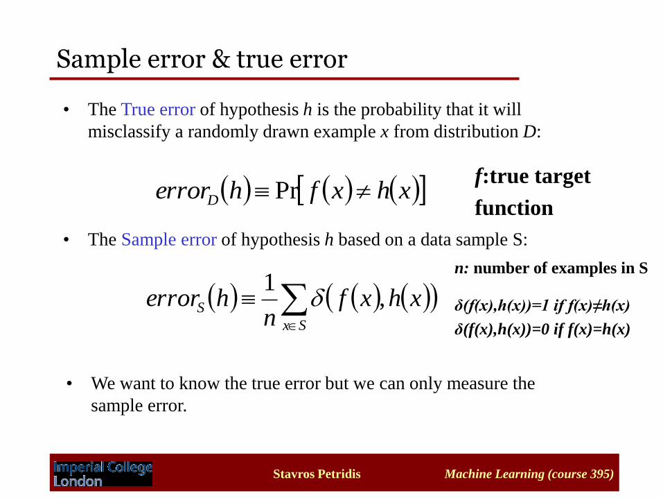
Sample error & true error

• The True error of hypothesis h is the probability that it will

misclassify a randomly drawn example x from distribution D:

xhxfherrorD Pr

• We want to know the true error but we can only measure the

sample error.

f:true target

function

• The Sample error of hypothesis h based on a data sample S:

Sx

S xhxfn

herror ,1

n: number of examples in S

δ(f(x),h(x))=1 if f(x)≠h(x)

δ(f(x),h(x))=0 if f(x)=h(x)


Sample Set Assumptions

• We assume that the sample S is drawn at random using the same

distribution D from which future examples will be drawn.

• Drawing an example from D does not influence the probability that

another example will be drawn next.

• Examples are independent of the hypothesis (classifier) h being tested.


Bernouli Process

• Let’s draw a random example from the distribution D (which generates

our examples). This is a Bernouli trial since there are only two

outcomes, the example will be either correctly classified or

misclassified.

• The probability of misclassification is p. Note also that p

is the true error.

• We draw n examples and count the number of misclassifications r

(corresponds to the number of heads). Sample error = r/n.

• If we repeat the same experiment another n times then r will be slightly

different.


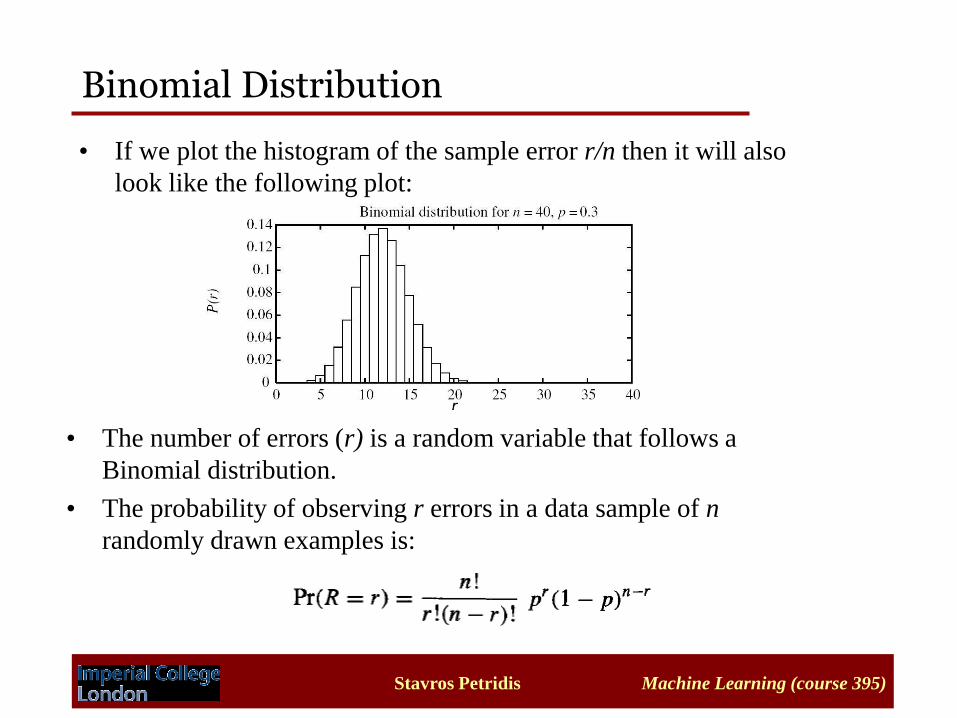
Binomial Distribution

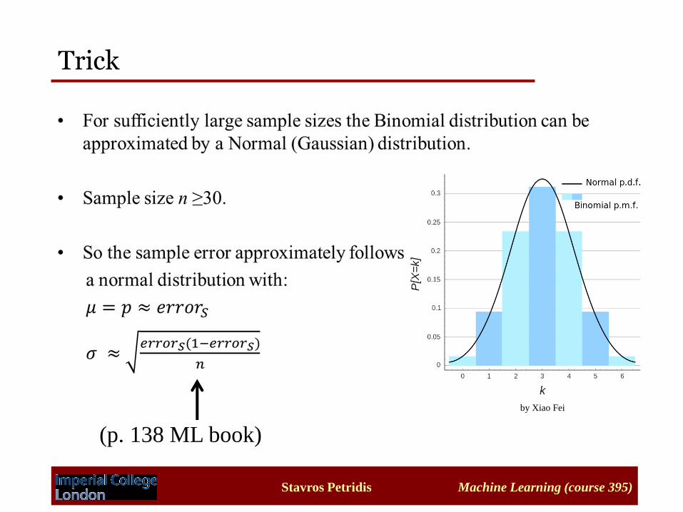
• If we plot the histogram of the sample error r/n then it will also

look like the following plot:

• The number of errors (r) is a random variable that follows a

Binomial distribution.

• The probability of observing r errors in a data sample of n

randomly drawn examples is:


Sample Error as Estimator

• True error = p

• Sample error = r/n

• Sample error is a random variable that follows a binomial

distribution.

• Estimator = random variable used to estimate some

parameter (in our case p) of the population from which the

sample is drawn.

• Sample error is called an estimator of the true error.

• Expected value of r = np (Exp. Val. Binomial distribution)

• Expected value of sample error = np/n =p.


• Q1: What is the best estimate of the accuracy over future examples

drawn from the same distribution?

• True error = p

• Expected value of sample error = np/n =p.

• The best estimate of the true error is the sample error.

Sample Error as Estimator


Confidence interval

• Q2: What is the probable error in this accuracy estimate? We want to

assess the confidence that we can have in this classification measure.

• What we really want to estimate is a confidence interval for the true

error.

• An N% confidence interval for some parameter p is an interval that

is expected with probability N% to contain p.

e.g. a 95% confidence interval [0.2,0.4] means that with probability

95% p lies between 0.2 and 0.4.


Trick

by Xiao Fei

(p. 138 ML book)


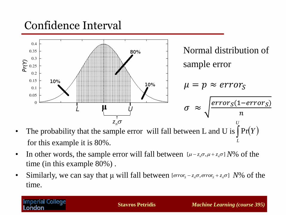
Confidence Interval

Normal distribution of

sample error

U

L

YPr• The probability that the sample error will fall between L and U is

for this example it is 80%.

• In other words, the sample error will fall between N% of the

time (in this example 80%) .

• Similarly, we can say that μ will fall between N% of the

time.

μ

nz

],[ nn zz

],[ nSnS zerrorzerror


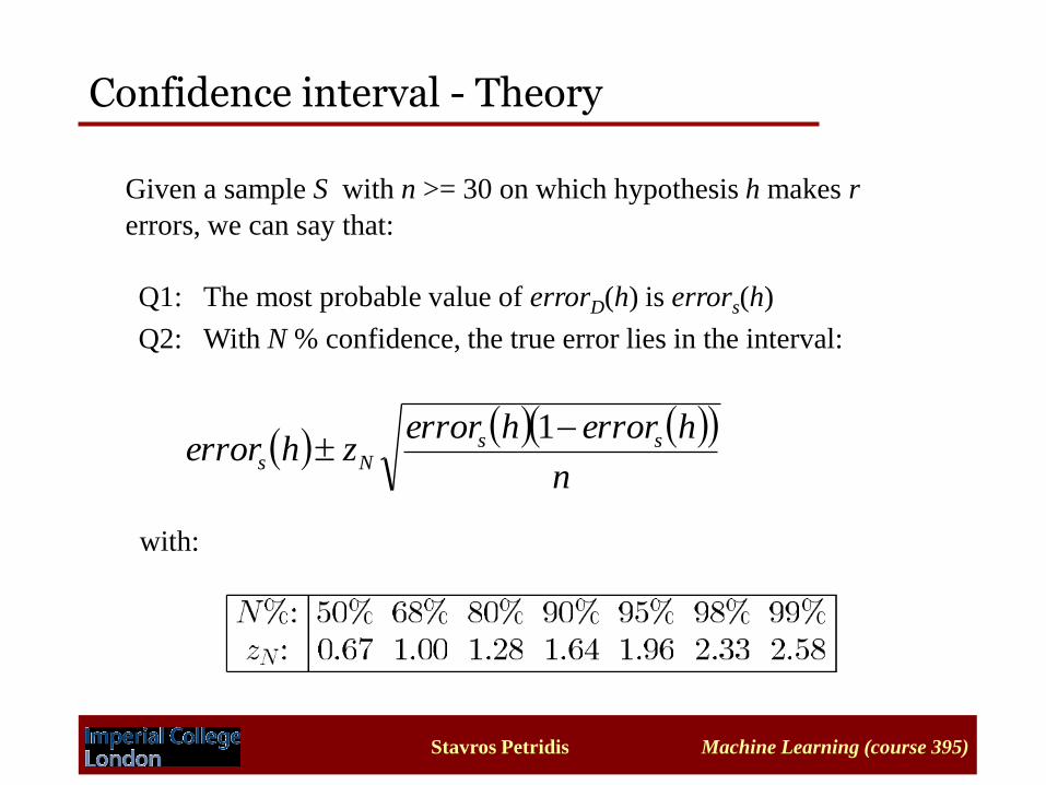
Confidence interval - Theory

Given a sample S with n >= 30 on which hypothesis h makes r

errors, we can say that:

Q1: The most probable value of errorD(h) is errors(h)

Q2: With N % confidence, the true error lies in the interval:

n

herrorherrorzherror ss

Ns

1

with:


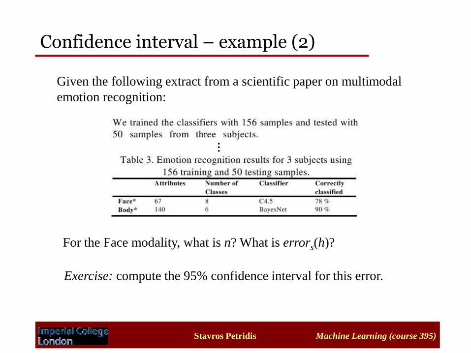
Confidence interval – example (2)

Given the following extract from a scientific paper on multimodal

emotion recognition:

For the Face modality, what is n? What is errors(h)?

Exercise: compute the 95% confidence interval for this error.


Confidence interval – example (3)

Given that errors(h)=0.22 and n= 50, and zN=1.96 for N = 95%, we can

now say that with 95% confidence errorD(h) will lie in the interval:

34.0,11.0

50

22.0122.096.122.0,

50

22.0122.096.122.0

What will happen when ? ¥®n


Comparing Two Algorithms

• Consider the distributions as the classification errors of two different

classifiers derived by cross-validation.

• The means of the distributions are not enough to say that one of the

classifiers is better!! In all cases the mean difference is the same.

• That’s why we need to run a statistical test to tell us if there is indeed a

difference between the two distributions.


Two-sample T-test

mn

t

yx

yx

22

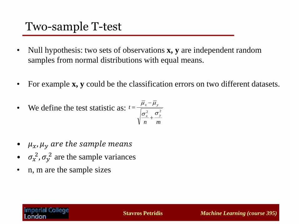
• Null hypothesis: two sets of observations x, y are independent random

samples from normal distributions with equal means.

• For example x, y could be the classification errors on two different datasets.

• We define the test statistic as:

• 𝜇𝑥, 𝜇𝑦 𝑎𝑟𝑒 𝑡ℎ𝑒 𝑠𝑎𝑚𝑝𝑙𝑒 𝑚𝑒𝑎𝑛𝑠

• 𝜎𝑥 2, 𝜎𝑦

2 are the sample variances

• n, m are the sample sizes


• Null hypothesis: the difference between the observations x-y are a random sample

from a normal distribution with 𝜇 = 0 and unknown variance.

• It’s called paired because the observations are matched, they are not independent.

• For example x, y could be the classification errors on the same folds of cross-

validation from two different algorithms. The test folds are the same, i.e. they are

matched.

• We define the test statistic as:

• 𝜇𝑥−𝑦 is the sample mean of the differences

• 𝜎𝑥−𝑦 2 is the sample variance of the differences.

• n is the sample size

Paired T-test

n

t

yx

yx

2


T-test

• The test statistic t will follow a t-distribution if the null hypothesis is true.

That is why it is called t-test.

• Once we compute the test statistic we also define a confidence level,

usually 95%.

Confidence Level

t is less than 1.717 with

probability 95%. Degrees of

freedom: number

of values that are

free to vary, e.g.

for paired t-test =

n-1.


T-test

• If the calculated t value is above the threshold chosen for statistical

significance then the null hypothesis that the two groups do not differ is

rejected in favour of the alternative hypothesis, which typically states that

the groups do differ.

• Significance level = 1 – confidence level, so usually 5%.

• Significance level α%: α times out of 100 you would find a statistically

significant difference between the distributions even if there was none. It

essentially defines our tolerance level.

• To summarise: we only have to compute t, set α and we use a lookup table

to check if our value t is higher than the value in the table. If yes, then our

sets of observations are different (null hypothesis rejected).

course 395: machine learning - lectures · stavros petridis machine learning (course 395) course...

Documents