092011

Research Paper

Christoph Schottmüller

Also available as TILEC DP 2011-041 | http://ssrn.com/abstract=1930864

Cost incentives for doctors:a double-edged sword

Cost incentives for doctors:

A double-edged sword∗

Christoph Schottmüller†

September 15, 2011

Abstract

Incentivicing doctors to take the costs of treatment into account in their prescription decision

could lead to lower health care expenditures and higher welfare. This paper shows that also the

opposite e�ects can result. The reason is a misalignment of doctor and patient incentives: Because

of health insurance, the patient does not take the costs of treatment fully into account. This

misalignment hampers communication between patient and doctor, e.g. the patient may overstate

the intensity of symptoms. It is shown that cost incentives for doctors increase welfare if (i)

the doctor's examination technology is su�ciently good or (ii) (marginal) costs of treatment are

high enough. Optimal health care systems should implement di�erent degrees of cost incentives

depending on type of disease and/or doctor.

JEL: D82, D83, I10

Keywords: cheap talk, communication, health insurance, market design

1. Introduction

It is well known that insurance creates moral hazard: In the health sector, insured people would like

to have more expensive treatments than socially optimal. On the other hand, treatments are normally

prescribed by doctors. If doctors took the costs of treatment into account in their treatment decision,

the moral hazard problem should disappear. The tradition in the medical profession, however, is to

view oneself as advocate of one's patients. Consequently, the patient's wellbeing is put �rst and costs

∗I want to thank Jan Boone for comments on an early draft of this paper.†Department of Economics, Tilec and CentER, Tilburg University, email: christophschottmueller@googlemail.com

1

are only secondary. What is more, doctors are often explicitly hostile towards cost incentives in doctor

remuneration. The German chamber of doctors, for instance, writes in its principles of health policy1

[. . . ] the role of the doctor as advocate for his patient must not be restricted [. . . ] The state

must not establish �nancial schemes (e.g. bonus-malus system) which could suggest to the

patient that materialistic, self-serving aspects are also of importance for medical decisions.

It is important to understand whether the doctors' concerns are mainly self-interested, e.g. worries

about reputation and pay, or whether �nancial incentives for doctors could have a negative impact

on social welfare. Put di�erently, can patient advocacy be interpreted as an e�cient institutional

response to the particular structure of the health care market? Answering this question will also give

some insight into the optimal design of health care markets. In particular, in which parts of the health

care system should cost incentives for doctors be employed and where are cost incentives less likely to

succeed?

This paper focuses on the communication between patient and doctor. The patient's input, e.g.

describing his symptoms and their intensity, is vital to reach the right diagnosis.2 The main mechanism

I explore in this paper is the following: Patients are (fully) insured. If doctors take costs into account

in their treatment decision, their objectives and the objectives of their patients are no longer aligned.3

Such a misalignment undermines the patient's trust in his doctor which in turn a�ects communication

negatively.4 More technically, in a setting where the patient has private information, e.g. about his

symptoms and their intensity, he has the possibility to exaggerate his symptoms (or their intensity)

in order to get a more expensive treatment. Of course, the doctor will anticipate such strategic

exaggerating. This anticipation gives the patient further incentives to exaggerate and so on. The

appropriate model to analyze such a �rat race� is the cheap talk framework. This paper will therefore

extend the canonical cheap talk model to the imperfect information setting typical for the health sector.

Although a complete breakdown of communication can be prevented, communication will be worse in

1Translation by the author. Original title and source: �Gesundheitspolitische Leitsätze der Ärzteschaft�Ulmer

Papier� Beschluss des deutschen Ärztetags 2008, Anlage 1, p. 6, http://www.bundesaerztekammer.de/downloads/

UlmerPapierDAET111.pdf2The importance of communication is also stressed in the aforementioned document of the German chamber of doctors

where it is stated that �health can neither be commanded nor produced since health depends crucially on the patient's

collaboration.� Also there is a whole string of the medical literature dealing with doctor-patient communication, see

Stewart (1995) for a survey.3Negative e�ects from cost incentives on the doctor-patient relationship are also established in the medical literature,

see for example Rodwin (1995), Kao et al. (1998) or Gallagher and Levinson (2004).4There is no doubt that patients understand this nexus: According to Gallagher et al. (2001) 73% of their respondents

dislike the idea of a cost control bonus for their doctor and 91% favor disclosure to the patient if such a bonus was in

place. Furthermore, 95% of those who dislike the bonus stated that the bonus would lower their trust in their physician.

2

equilibrium because of the misalignment of interests, i.e. less information is transmitted from patient

to doctor. It is shown that this communication e�ect can make a system without cost incentives

preferable from a social welfare point of view. If the patient's collaboration is hardly needed, a system

with cost incentives is preferable. For example, a doctor can easily establish that a patient has a

broken leg by having an X-ray. The symptoms reported by the patient are less important in this case.

If, on the other hand, an illness might have a psychological background, the patient's collaboration is

essential and a system without cost incentives might be preferable.

The main idea of the paper is a tradeo� between having the best information to base the decision on

and having the socially best decision rule. A related tradeo� is known in organization theory. Alonso

et al. (2008) ask how much autonomy division managers should have. Giving division managers more

autonomy results in better information use in decision making but less coordination across divisions. In

my paper, the only way to get better information (from the patient) is a socially less desirable decision

rule for the doctor. In both papers, there is a tradeo� between the quality of information and the

quality of the decision rule (for a given information structure). The downside of an informed decision

in Alonso et al. (2008) is a lack of coordination while in my paper it will be the neglect of costs. A

major technical di�erence between the papers is that division managers (headquarters manager) have

full (no) information in Alonso et al. (2008) while doctor and patient will both receive a noisy signal

in my model. This setup seems to be closer to reality in the health sector.

From a technical point of view the paper contributes to the cheap talk literature following the

seminal paper by Crawford and Sobel (1982). Their model is extended in de Barreda (2010) to a setup

where the decision maker receives a noisy signal. My paper generalizes further by substituting the

perfect information on the sender/expert/patient side by a noisy signal.

This paper complements existing literature on the design of health care systems. Early contribu-

tions as Arrow (1963) and Pauly (1968) already point out the moral hazard caused by health insurance:

Insured patients might overconsume treatment from a social welfare perspective because they are in-

sured. Ma and McGuire (1997) introduce the physician as an additional player and analyze contractual

di�culties in the health market. In particular, health outcome and doctor's e�ort are non-contractible

and even the quantity of care consumed can be subject to misreporting. Ma and McGuire (1997)

analyze how these contractual constraints in�uence optimal contracts between insurance and patient

as well as between insurance and physician. My paper focuses on a di�erent kind of constraint, i.e.

a constraint in information transmission arising in the communication between doctor and patient.

It will be shown that the necessity of information transmission between patient and doctor might

constrain the power of the incentive scheme o�ered to the doctor.

3

Obviously related is the literature on physician compensation and managed care. In his survey

Glied (2000) mentions two problems of �supply-side cost sharing,� i.e. cost incentives for physicians:

(i) underprovision of necessary services and (ii) strong incentives to avoid costly cases. In this context

my paper adds a third problem: Hampered information transmission between doctor and patient.

Furthermore, my paper provides one possible explanation for the ambiguous cost e�ect of managed

care mentioned in Glied (2000).

The medical literature contains statements like �payment arrangements could signi�cantly under-

mine patients' beliefs that their physicians are acting as their agents� (Mechanic and Schlesinger, 1996)

and emphasizes that there should be no con�ict of interest between patient and doctor (Emanuel and

Dubler, 1995). Kao et al. (1998) �nd that patients trust their physician less if the physician is cap-

itated than when he is payed on a fee for service basis. Physicians are also less satis�ed with their

relationships with capitated patients compared to their average patient (Kerr et al., 1997). My paper

contributes by formalizing why trust, interpreted as shared objectives, is vital for the patient-physician

relationship. Such a formalization is interesting for two reasons: First, it allows for both costs (less

trust) and bene�ts (less overtreatment) of cost incentives. Second, one can obtain results concern-

ing the optimal design of health care systems, i.e. where in the health system are aligned interests

especially important and where could cost incentives improve welfare.

The next section introduces the model and is followed by a simple numerical example. This example

illustrates the main points. Section 4 analyzes a general model and answers the question: When do

cost incentives work? The �nal section concludes by discussing certain assumptions and pointing out

testable predictions as well as possible applications in di�erent areas.

2. Formal setting

Patient and doctor have a common prior F over the set of all possible health states of the patient. The

set of health states is denoted by Θ. A health state can be interpreted either as the severity of a given

disease or as a set containing di�erent diseases. The patient receives a private signal σp ∈ Σp about

his health state. In practice this signal can be interpreted as the symptoms a patient can report to his

doctor or as the intensity of his symptoms. The doctor receives also a private signal σd ∈ Σd about

the patient's health. This signal can be interpreted as the result of the doctor's examination, e.g. his

interpretation of an X-ray photograph or listening to the patient's heartbeat. Given the health state,

there is a distribution G(σp, σd|θ) of signals which is common knowledge. Put di�erently, G(σp, σd|θ)

gives the probabilities that a patient (doctor) receives signal σp (σd) given a health state θ.

4

The timing is the following: First, the patient's health state is determined by nature. This health

state is unknown to doctor and patient. Second, doctor and patient receive their signals σ = (σp, σd)

which correspond to the true health state through G. Third, the patient can send a message, e.g.

communicating his signal, to the doctor. Fourth, the doctor determines a treatment τ from a set of

available treatments. The costs of the treatment c(τ) are paid for by the patient's insurance.

Utility of the patient depends only on his true health state θ ∈ Θ and the treatment τ . In

particular, a patient's well being does in the end not depend on the signals. For the doctor, I look at

two scenarios: Either the doctor has �no cost incentives� which means that he makes his treatment

decision to maximize the patient's utility or he is �cost sensitive� (or �has cost incentives�) with which

I mean that he maximizes social welfare. Social welfare is the patient's utility minus costs. The

perspective of the paper is therefore eventually the perspective of a (benevolent) designer of the health

system, e.g. a government or an insurance plan, who has to determine which kind of incentives he

gives to the doctor.

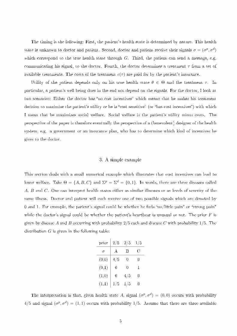
3. A simple example

This section deals with a small numerical example which illustrates that cost incentives can lead to

lower welfare. Take Θ = {A,B,C} and Σp = Σd = {0, 1}. In words, there are three diseases called

A, B and C. One can interpret health states either as similar illnesses or as levels of severity of the

same illness. Doctor and patient will each receive one of two possible signals which are denoted by

0 and 1. For example, the patient's signal could be whether he feels �no/little pain� or �strong pain�

while the doctor's signal could be whether the patient's heartbeat is unusual or not. The prior F is

given by disease A and B occurring with probability 2/5 each and disease C with probability 1/5. The

distribution G is given in the following table:

prior 2/5 2/5 1/5

σ A B C

(0,0) 4/5 0 0

(0,1) 0 0 1

(1,0) 0 4/5 0

(1,1) 1/5 1/5 0

The interpretation is that, given health state A, signal (σp, σd) = (0, 0) occurs with probability

4/5 and signal (σp, σd) = (1, 1) occurs with probability 1/5. Assume that there are three available

5

treatments which are denoted by a, b and c. The patient's utility and the costs of each treatment are

given in the following table:

A B C costs

a 8 5 8 5

b 10 10 9 8

c 1 1 10 0

To illustrate: A patient with disease A receiving treatment a has a utility of 8. Treatment a costs

5. Therefore, welfare would be 8− 5 = 3 in this situation.

One interpretation is that �disease� C is being healthy and treatment c is the option �no treat-

ment�. Treatment b is a very e�ective but also very expensive treatment while a is not so e�ective but

substantially cheaper. A quick calculation shows that treatment a is welfare maximizing where welfare

is de�ned by patient utility minus costs. The same is true for b in health state B and c in C.

3.1. No cost incentives

If the doctor has no cost incentives, the incentives of doctor and patient are aligned. The patient will

therefore communicate his true signal σp in equilibrium.5 The doctor can then base his decision on

both signals and maximizes gross consumer surplus. Hence, the doctor knows the disease whenever

the signals are (0, 0), (0, 1) or (1, 0). If the signal is (1, 1), the doctor assigns equal probabilities to

disease A and B. This leads to the following optimal decisions: (0, 0) → b, (0, 1) → c, (1, 0) → b and

(1, 1)→ b

Expected welfare is therefore:6

Wnci =16

50(10− 8) +

1

510 +

16

50(10− 8) +

4

50(10− 8) +

4

50(10− 8) =

180

50(1)

3.2. Cost sensitive doctor

If the doctor is cost sensitive, his preferred decisions (if he knew both signals) would be: (0, 0) → a,

(0, 1) → c, (1, 0) → b and (1, 1) → b. Hence, there is a con�ict between the patient and the doctor

whenever the signal is (0, 0): The doctor prefers treatment a while the patient prefers b. Next, I write

down the optimal decision of the doctor if he only knows his own signal σd. If σd = 0, he assigns equal

5In principle, there is also a pooling equilibrium in which the doctor takes only his own signal into account and the

patient sends the same message regardless of his signal. However, this equilibrium is Pareto dominated and does not

seem very realistic.6Just to illustrate: The �rst term is the probability of being in state A and receiving the signal (0, 0), i.e. 2/5 ∗ 4/5,

multiplied with the utility of the resulting treatment b in state A, i.e. 10, minus the costs of this treatment, i.e. 8.

6

probability to disease A and B. Therefore, the optimal treatment is b. If σd = 1, he assigns probability

2/9 to disease A, 2/9 to disease B and 5/9 to disease C. It is straightforward to calculate that in this

case the optimal treatment is c.

In principle, there could be two kinds of equilibrium: First, a separating equilibrium in which the

patient truthfully reports his signal to the doctor, i.e. the two signals are separated. Second, a pooling

equilibrium in which the patient sends the same message regardless of his signal.

Suppose there is a separating equilibrium, i.e. the patient communicates his signal σp truthfully

to the doctor in equilibrium. The doctor will then implement the welfare maximizing treatment

knowing both signals. If σp = 0, the patient expects�given his signal�to get a utility of utruth =

8/13∗8+5/13∗10 = 114/13.7 If however the patient lied and communicated σp = 1, the doctor would

implement treatment b and the patient's expected utility would be ulie = 8/13∗10+5/13∗9 = 125/13.

Hence, lying pays o� for the agent and there cannot be a separating equilibrium.

Consequently, there is a pooling equilibrium in which the doctor uses only his own signal. Welfare

is then

W c =16

50(10− 8) +

1

510 +

16

50(10− 8) +

4

501 +

4

501 =

172

50(2)

Since W c < Wnci, cost incentives reduce welfare in this example. Nevertheless, costs are lower if

the doctor is cost sensitive since the signal (1, 1) leads to the low cost treatment c while b is prescribed

without cost incentives. The driving force behind this result are the con�icting objectives of patient

and doctor which result in a break down of communication.

3.3. Variation I: Restricting the choice set

Interestingly, there is an easy �x in this example: Suppose, the health authority does not clear treatment

a. Hence, treatment a is not available. But then there is no con�ict between doctor and patient as

even a cost sensitive doctor will now prescribe b if the signal (0, 0) occurs. Unfortunately, this means

that cost incentives simply do not matter/work: Every signal leads to the same treatment with and

without cost incentives. Furthermore, this trick will not always work: Amend the example above with

a disease D which can be identi�ed with certainty (so there would be a signal (2, 2) which occurs if and

only if the health state is D). If in this state D treatment a is by far superior to all other treatments,

a health authority banning treatment a would reduce welfare.

7Given σp = 0, the patient assigns probability 8/13 to health state A with signal σ = (0, 0) which leads to treatment

a. With the counter probability 5/13, he expects state C with signal σ = (0, 1) and treatment c.

7

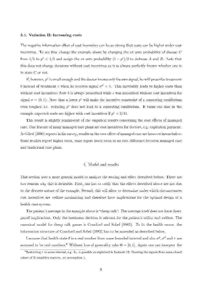
3.4. Variation II: Increasing costs

The negative information e�ect of cost incentives can be so strong that costs can be higher under cost

incentives. To see this, change the example above by changing the ex ante probability of disease C

from 1/5 to pc < 1/5 and assign the ex ante probability (1 − pc)/2 to sickness A and B. Note that

this does not change decisions without cost incentives as it is always perfectly known whether one is

in state C or not.

If, however, pc is small enough and the doctor knows only his own signal, he will prescribe treatment

b instead of treatment c when he receives signal σd = 1. This inevitably leads to higher costs than

without cost incentives: Now b is always prescribed while c was prescribed without cost incentives for

signal σ = (0, 1). Note that a lower pc will make the incentive constraint of a separating equilibrium

even tougher, i.e. reducing pc does not lead to a separating equilibrium. It turns out that in the

example expected costs are higher with cost incentives if pc < 2/41.

This result is slightly reminiscent of the empirical results concerning the cost e�ects of managed

care. One feature of many managed care plans are cost incentives for doctors, e.g. capitation payment.

As Glied (2000) reports in his survey, results on the cost e�ect of managed care are however inconclusive:

Some studies report higher costs, some report lower costs or no cost di�erence between managed care

and traditional care plans.

4. Model and results

This section uses a more general model to analyze the setting and e�ect described before. There are

two reasons why this is desirable: First, one has to verify that the e�ects described above are not due

to the discrete nature of the example. Second, this will allow to determine under which circumstances

cost incentives are welfare maximizing and therefore have implications for the optimal design of a

health care system.

The patient's message in the example above is �cheap talk�: The message itself does not have direct

payo� implications. Only the treatment decision is relevant for the patient's utility and welfare. The

canonical model for cheap talk games is Crawford and Sobel (1982). To �t the health sector, the

information structure of Crawford and Sobel (1982) has to be amended as described below.

I assume that health state θ is a real number from some bounded interval and also σp, σd and τ are

assumed to be real numbers.8 Without loss of generality take Θ = [0, 1]. Again one can interpret the

8Restricting τ to some interval, e.g. R+ is possible as explained in footnote 13. Drawing the signals from some closed

subset of R simpli�es matters, see assumption 1.

8

health state either as the severity of a given illness or one views Θ as a continuum of illnesses. Higher

signals are assumed to imply higher expected states. To make this formal de�ne by H(θ|σp, σd) the

cumulative distribution function which gives the probability that the state is below θ given signals σp

and σd. This distribution is derived from F (θ) and G(σp, σd|θ) using Bayes' rule. The assumption is

that H(θ|σp, σd) �rst order stochastically dominates H(θ|σp′, σd′) whenever σd ≥ σd′ and σp ≥ σp′. In

words, a higher signal implies that higher health states are more likely to occur.

Patient utility u(θ−τ) is a function of �distance� between health state and treatment. It is assumed

that the patient is fully insured, i.e. costs of treatment do not enter his utility function. Assume that

u(θ − τ) is two times continuously di�erentiable, strictly concave and attains its maximum at 0. Put

di�erently, patient utility is maximized if τ = θ and is lower the further away treatment τ is from

this ideal treatment. It is not assumed that u(·) is symmetric and therefore over- and undertreatment

might a�ect utility in di�erent ways. The cost function c(τ) is strictly increasing and marginal costs

are bounded away from 0, i.e. c′(τ) ≥ δ ∀τ for some δ > 0. This last assumption implies that the

patient's utility is never aligned with the social objective or, put di�erently, the patient always prefers

a more expensive treatment than socially optimal because he is insured. If there was no such con�ict,

cost incentives would simply not matter for the outcome. Consequently, introducing cost incentives

could not even help to reduce costs.

I use Perfect Bayesian Nash Equilibrium as solution concept. After observing his signal σp a patient

updates his beliefs about his health state θ and about the doctor's signal. Given σp, a strategy for

the patient is a probability distribution over Σp denoted by q(m|σp).9 This distribution gives the

probability of reporting m ∈ Σp when the true signal is σp. For illustration purposes, think of a

partition equilibrium in which patients with signals in, say, [0.3, 0.4] are bunched, i.e. send the same

message. In this case q(m|σp) could be a uniform distribution over [0.3, 0.4] for all σp ∈ [0.3, 0.4].

Given his signal σd and the message he receives from the patient, the doctor updates his beliefs about

the health state of the patient θ and chooses his preferred treatment. For simplicity, I assume that

u(θ− τ)− c(τ) is strictly concave in τ which implies that there is a unique socially e�cient treatment

τw. This assumption is, for example, satis�ed if c(τ) is linear or convex. Hence, the doctor will always

have a unique preferred treatment which I denote by τd(m,σd). The strategies (q(m|σp), τd(m,σd))

form an equilibrium if:

1. For each σp, q(m|σp) is a distribution, i.e.∫ 1

0 q(m|σp) dm = 1, and if q(m∗|σp) > 0 then

m∗ ∈ argmaxm∫ 1

0

∫Σd u(|θ − τd(m,σd)|) dP (θ, σd|σp) where P (θ, σd|σp) is the distribution of

(θ, σd) derived from G(σp, σd|θ) and F (θ) conditional on observing σp and using Bayes' rule.10

9For notational convenience q(m|σp) is a probability density function but mass points can be easily accommodated.10Note that the patient takes expectations not only over the health state but also over the doctor's signal because σd

9

2. For each m and σd treatment maximizes the doctor's objective. For the cost sensitive doctor

this means that τd(m,σd) ∈ argmaxτ∫ 1

0 [u(θ− τ)− c(τ)] dH(θ|m,σd) where with a slight abuse

of notation H(θ|m,σd) is the distribution of the health state conditional on observing σd and m

using by Bayes' rule (given G(σp, σd|θ), F (θ) and q(m|σp)). Without cost incentives τd(m,σd) ∈

argmaxτ∫ 1

0 u(θ − τ) dH(θ|m,σd).

In words, the �rst condition says that the patient reports with positive probability only signals max-

imizing his utility given the strategy of the doctor. The second condition establishes that the doctor

uses an optimal strategy given the patient's equilibrium behavior.

For the analysis of this model the following technical assumption proves to be useful. Note that

the boundedness part is automatically satis�ed if Hσp is continuous and the signal σ is drawn from a

closed set, i.e. if Σp and Σd are closed intervals.

Assumption 1. H(θ|σp, σd) is di�erentiable in σp and |Hσp(θ|σp, σd)| is bounded from above by some

M > 0. At all states where H(θ|σp, σd) has a density h(θ|σp, σd), this density is also di�erentiable in

σp and hσp is bounded.

Put di�erently, beliefs about the true health state do not change too sharply if the patient's signal

changes marginally. Note that slightly irregular distribution, e.g. with mass points at a �healthy state�

θ = 0, can be allowed. Assumption 1 simpli�es the analysis by ensuring that the doctor's treatment

decision is di�erentiable in the patient's signal.

The game is then similar to the information transmission model of Crawford and Sobel (1982) with

three additional twists: First, the doctor (receiver in the language of Crawford and Sobel) receives

a signal while he is completely ignorant in Crawford and Sobel (1982). Second, the patient (sender)

does not know the state of the world. Instead he has a noisy signal. Third, the divergence of interests

between doctor (receiver) and patient (sender) is not �xed but depends on the treatment (decision).

The following proposition extends results from Crawford and Sobel (1982) to this more general setting.

Proposition 1. With cost incentives, there exists no separating equilibrium. There exist partitioning

equilibria on the range of σp. Each part of this partition has a minimum length κ which is bounded

away from zero. If Σp is bounded, the number of parts in the partition is bounded from above.

Proof. see appendix

The intuition is the following: In equilibrium a patient cannot tell his true signal to the doctor.

If he did, the doctor would prescribe a treatment that is �too cheap� from the patient's point of view

(as he does not care about costs). Hence, the patient would have an incentive to overstate his signal.

will in�uence the doctor's treatment decision.

10

In practice, this would mean to claim additional symptoms or to overstate the intensity of existing

symptoms. What happens in equilibrium is that the patient's signal range is partitioned and the patient

reports in which part of the partition his signal lies. The doctor does not know the precise signal of the

patient but gets a rough idea which he takes into consideration when choosing the treatment. Because

of the partitioning, a patient can no longer overstate his signal �a little bit�. If the patient deviated by

reporting a higher part of the partition, he would get a substantially higher treatment. In equilibrium

he will not deviate because he expects this treatment to be too high. In practice one could interpret

this in the following two ways: First, a patient does not want to report symptoms that are too much

di�erent from the real ones as this could mislead the doctor, i.e. result in treating the wrong illness.

Second, extreme overstatement of symptoms could result in too strong medication with severe side

e�ects. Hence, the patient does not want to overstate his existing symptoms too much.

It is also clear that the partition cannot be arbitrarily �ne: If the parts are too small, then over-

stating one's signal �a little bit� is again possible. This explains the minimum length statement in the

proposition. The minimum part length immediately implies that the number of parts is bounded if

the interval from which patient signals are drawn is bounded.

The mechanism through which cost incentives can harm welfare is the same as in the example

of section 3: If the objectives of doctor and patient are di�erent, the patient has an incentive to

use his information strategically to get the more expensive treatment he wants. In equilibrium, the

doctor will have less information (partitioning of signal range) compared to the situation without cost

incentives. Consequently, he is more prone to make inappropriate treatment decisions. In short, there

are two e�ects when introducing cost incentives: First, costs are taken into account which, ceteris

paribus, decreases costs and increases welfare. Put di�erently, the doctor stops prescribing excessively

expensive treatments. Second, communication and therefore the information of the doctor is worse.

Hence, treatment decisions are less accurate which reduces welfare. Whether the cost or the information

e�ect dominates is ex ante unclear. The following propositions show that in two extreme cases the

cost e�ect dominates and therefore cost incentives lead to higher welfare than no cost incentives.

Proposition 2. Welfare is higher with cost incentives if the doctor's signal is su�ciently informative.

That is, given G(σp, σd|θ), there exists an ε > 0 such that cost incentives lead to higher welfare

than no cost incentives if the doctor's signal is drawn from εG(σp, σd|θ) + (1 − ε)1θ where 1θ is a

distribution putting all probability mass on θ. Cost incentives lead also to higher welfare if the patient's

signal is su�ciently uninformative, i.e. for ε > 0 small enough if the patient's signal is drawn from

εG(σp, σd|θ) + (1− ε)Uθ where Uθ is the uniform distribution over [0, 1].

Proof. see appendix

11

This result is intuitive: If the doctor is able to determine the patient's health state almost on his

own, i.e. without knowing the patient's signal, then the patient's signal is useless. Therefore, the

information e�ect of introducing cost incentives is small while the cost e�ect is still there.

One interpretation of proposition 2 is that cost incentives become eventually more attractive with

medical progress. This holds at least true if medical progress implies better diagnosis possibilities

for doctors. Consequently, one might then expect to see more cost incentive elements in health care

systems over time.

A second interpretation is that some specialists optimally should have cost incentives while others

should not. A radiologist or a trauma surgeon will normally base his decisions on his own examination

and less on the patient's report.11 This might be less true for an internist or a general practitioner.

A related third interpretation is that an optimal health care system should incorporate selective

cost incentives. More precisely, cost incentives should be applied for the treatment of diseases where

the doctor's information is relatively more important than the patient's information.

Proposition 3. Cost incentives lead to higher welfare than no cost incentives if social and private

objectives di�er su�ciently. That is, for any given information structure and cost function c(τ) there

exists an α > 0 such that cost incentives lead to higher welfare than no cost incentives under the cost

function αc(τ).

Proof. see appendix

The intuition is that the cost e�ect will become dominant if (marginal) costs are high enough.

Consequently, the information loss due to cost incentives is negligible compared to the cost e�ect.

In line with previous interpretations cost incentives are especially useful for specialists dealing with

high cost treatments on a regular basis. Also diseases involving high cost treatment on a regular basis

are especially well suited for cost incentives.

The previous propositions illustrate when cost incentives are superior to no cost incentives. To

conclude this section, I want to give an example where no cost incentives are superior to cost incentives.

In fact, I can use the same example as Crawford and Sobel (1982) which is attractive for two reasons:

First, it is very simple and allows therefore for an analytical solution. Second, it has been used

repeatedly in the cheap talk literature and has become a benchmark example there.

Example. Health states are uniformly distributed on [0, 1]. The patient has perfect knowledge of the

health state while the doctor's signal is completely uninformative. Assume that the patient's utility

function is a quadratic loss function, i.e. u(θ, τ) = −(θ − τ)2, and that the cost function is linear in

11Another example of this category is the veterinarian or to quote Will Rogers: �The best doctor in the world is the

veterinarian. He can't ask his patients what is the matter-he's got to just know.�

12

treatment, i.e. c(τ) = ατ . Given the information that σp (which is now the true health state) is in the

interval (s1, s2), the optimal treatment decision for a doctor with cost incentives is τ = s1+s2−α2 . With

α = 1/10 the model is mathematically equivalent to the example in Crawford and Sobel (1982). It is

shown there that the �nest possible equilibrium partition is (0, 2/15, 7/15, 1), i.e. a patient will report

whether his signal is in [0, 2/15) or in [2/15, 7/15) or in [7/15, 1]. Utility of a patient with state θ in

[0, 2/15) is given by −(1/60 − θ)2, with θ ∈ (2/15, 7/15) utility is −(1/4 − θ)2 and with θ ∈ (7/15, 1)

utility is −(41/60− θ)2. Expected consumer utility in this partition equilibrium is therefore

EU =

∫ 2/15

0−(

1

60− θ)2

dθ +

∫ 7/15

2/15−(

1

4− θ)2

dθ +

∫ 1

7/15−(

41

60− θ)2

dθ ≈ −0.01058

while expected costs are

EC =1

10

(2

15

1

60+

5

15

15

60+

8

15

41

60

)= 0.045.

Hence expected welfare is −0.01058− 0.045 = −0.05558. Note that this is an upper bound on welfare:

Of course, there are also equilibria with partitions consisting of only two parts or one part. It is easy

to check that these equilibria result in lower welfare.

Without cost incentives the patient will truthfully reveal his signal and therefore communicate the

true health state to the doctor. Consequently, τ = θ and consumer welfare is 0. Expected costs are

1100.5 = 0.05 which results in expected welfare of −0.05. Therefore, no cost incentives lead to higher

welfare than cost incentives.

5. Discussion and conclusion

Introducing cost incentives for doctors turns out to be a double edged sword: On the one hand, taking

costs into consideration should avoid the prescription of too expensive treatments. On the other hand,

misalignment of patient's and doctor's incentives will hamper communication between the two: The

patient has an incentive to exaggerate and in equilibrium this leads to signal bunching. Consequently,

the doctor has worse information and is less likely to assess the patient's health state correctly. Knowing

about the uncertainty he might even choose more expensive treatments to be on the safe side. In a

numerical example, this can lead to higher costs than under no cost incentives (see section 3).

If costs are very high or if the doctor is able to assess the health state very accurately given only his

signal, cost incentives are the welfare maximizing policy. This shows that an optimal health care system

will use di�erent degrees of cost incentives in di�erent circumstances. In practice, cost incentives could

di�er across diseases and across specialists.

Although the model is stylized, it allows to formalize the idea that trust is important in the patient-

13

doctor relationship. A lack of trust reduces the quality of communication and eventually the quality

of the doctor's diagnosis. This e�ect could constrain contracting between insurances and doctors.

Note that some seemingly strong assumptions are actually not very restrictive: The concentration

on two extreme cases where the doctor either maximizes patient utility or total welfare is obviously

not realistic. The main e�ect, that diverging objectives lead to worse communication, however, holds

true whenever the doctor cares more about costs than the patient. By the same argument, it is not

restrictive to assume full indemnity insurance: The main point is that the patient does not bear the

full social costs which is a feature of any form of insurance. The results do therefore not depend on a

speci�c form of insurance. One can interpret the costs c(τ) simply as the part of treatment costs paid

by the patient's health insurance.

In some sense, the model is a best case scenario for the benevolent designer: He can freely set the

doctor's incentives without incurring any costs. In practice setting up an incentive scheme for doctors

might actually be costly. Doctors might also not respond immediately because of previously formed

habits. It is therefore even more remarkable that the designer might not want to give cost incentives

to the doctor.

The model gives several testable predictions. Quality of diagnosis should decrease after an intro-

duction of cost incentives for doctors. Such a quality decrease could be re�ected in the data in di�erent

ways: First, therapies could be changed more often (if the doctor realizes the error at a later stage).

Second, patients with a given diagnosis-treatment pair will be treated less successfully (e.g. take longer

to recover) because some receive the wrong treatment due to a wrong diagnosis. These e�ects should

be more pronounced for specialists and diseases where patient input is vital for the diagnosis. If trust

re�ects the willingness to communicate, one should expect patient's trust in their doctor to be lower

when their doctor has cost incentives. This last result is indeed con�rmed by the health literature, see

for example Kao et al. (1998).

More abstract, a welfare maximizing sponsor (say a benevolent government) might prefer a decision

maker (doctor) who shares his preferences not with the sponsor but with the patient. In a broader

context an agent might bene�t from surrendering his interests when information provision by another

party is important. This could have applications in other contexts like mediation: A mediator with

decision power who shares the interests of another party might be preferable to making the decision

oneself.

In general, shared objectives proof to be vital for information provision. Patient advocacy can

therefore be seen as an institutional response to the importance of information provision by patients.

Consequently, one might expect similar institutions to emerge whenever information provision by

14

a�ected parties is vital. In this context, the relationship between a lawyer and his client could serve

as an additional example.

15

References

Alonso, R., W. Dessein, and N. Matouschek (2008). When does coordination require centralization?

American Economic Review 98 (1), 145�179.

Arrow, K. (1963). Uncertainty and the welfare economics of medical care. American Economic Re-

view 53 (5), 941�973.

Crawford, V. and J. Sobel (1982). Strategic information transmission. Econometrica, 1431�1451.

de Barreda, I. (2010). Cheap talk with two-sided private information. London School of Economics;

mimeo.

Emanuel, E. and N. Dubler (1995). Preserving the physician-patient relationship in the era of managed

care. JAMA: Journal of the American Medical Association 273 (4), 323�329.

Gallagher, T. and W. Levinson (2004). A prescription for protecting the doctor-patient relationship.

American Journal of Managed Care 10 (2; part 1), 61�68.

Gallagher, T., R. St Peter, M. Chesney, and B. Lo (2001). Patients attitudes toward cost control

bonuses for managed care physicians. Health A�airs 20 (2), 186�192.

Glied, S. (2000). Managed care. Volume 1, chapter 13 of Handbook of Health Economics, pp. 707�753.

Elsevier.

Kao, A., D. Green, A. Zaslavsky, J. Koplan, and P. Cleary (1998). The relationship between method of

physician payment and patient trust. JAMA: Journal of the American Medical Association 280 (19),

1708�1714.

Kerr, E., R. Hays, B. Mittman, A. Siu, B. Leake, and R. Brook (1997). Primary care physicians'

satisfaction with quality of care in california capitated medical groups. JAMA: Journal of the

American Medical Association 278 (4), 308�312.

Ma, C. and T. McGuire (1997). Optimal health insurance and provider payment. American Economic

Review 87 (4), 685�704.

Mechanic, D. and M. Schlesinger (1996). The impact of managed care on patients' trust in medical

care and their physicians. JAMA: Journal of the American Medical Association 275 (21), 1693�1697.

Pauly, M. (1968). The economics of moral hazard: comment. American Economic Review 58 (3),

531�537.

16

Rodwin, M. (1995). Con�icts in managed care. New England Journal of Medicine 332 (9), 604�607.

Stewart, M. (1995). E�ective physician-patient communication and health outcomes: a review. CMAJ:

Canadian Medical Association Journal 152 (9), 1423�1433.

17

Appendix

Proof of proposition 1: The proof proceeds in a number of steps. The �rst three steps establish

that there cannot be a separating equilibrium, i.e. there is no equilibrium in which a patient always

reports his true signal. Consequently, patients with some signals are bunched together. Patients in one

�bunch� (one part of a partition of the signal range) send the same report to the doctor. Steps four

and �ve establish that each part of a partition must have minimum length, i.e. the partition cannot

be arbitrarily �ne.

The �rst step is to show that there exists a b > 0 such that argmaxτ∫ 1

0 [u(θ−τ)−c(τ)] dH(θ|m,σd)+

b ≤ argmaxτ∫ 1

0 u(θ − τ) dH(θ|m,σd) for a given equilibrium strategy q(m|σp); i.e. the patient would

opt for an at least b higher treatment than a cost sensitive doctor if he chose (and had the same

information). This follows from the �rst order conditions corresponding to the two argmax expressions

∫ 1

0−u′(θ − τ) dH(θ|m,σd) =

c′(τ)

0

. (3)

Since the left hand side is strictly decreasing in τ and c′(τ) ≥ δ the claim follows as u′(·) is continuous.

Therefore, the left hand side of (3) is continuous in τ and also strictly decreasing in τ . This argument

is for a given (m,σd) but the in�mum of all these b over (m,σd) will also be strictly positive. To

establish this, it is su�cient to show that the derivative of the left hand side of (3) with respect to τ

is bounded:12 Since u′(θ− x) > 0 for x ≥ 1 and any θ ∈ [0, 1], the optimal treatment is bounded from

above by 1. Furthermore, the optimal treatment is bounded from below by τ solving u′(−τ) = c′(τ),

i.e. the optimal treatment if the doctor knew that θ = 0. Therefore −1 ≤ θ − τ ≤ 1 − τ . By the

continuity of u′′(·) and the compactness of [−1, 1− τ ], u′′(·) is bounded on this interval. Consequently,

the derivative of the left hand side of (3) is a weighted (by the distribution H(·)) average of a bounded

function and therefore bounded. Denote by B > 0 such a bound on the derivative of the left hand side

of (3). Then we can choose b = δ/B.13

Second, the patient's expected utility is under separating higher under a slightly higher decision

than the cost sensitive doctor takes. From the �rst step and the strict concavity of u(·) it follows that

any treatment in (τd, τd + b) yields a higher expected utility for the patient than τd.

12Just to illustrate why boundedness is su�cient: Say the derivative of the left hand side of (3) is between 0 and −B.

Since this left hand side is di�erentiable, the two τ solving (3) with the right hand side equal to zero and equal to c′(τ)

have to di�er by at least δ/B.13If the treatment is restricted to be larger than, say, 0, the argument still holds true as long as H(0|0, 0) < 1. A

patient will then always desire a treatment that is strictly bounded away from 0. Therefore, interests of patient and

doctor are not aligned even if the constraint τ ≥ 0 is binding.

18

Third, in a hypothetical separating equilibrium the patient attains a higher utility by misrepresent-

ing slightly upwards as the doctor will increase his decision uniformly continuously in σp. The implicit

function theorem gives for a hypothetical separating equilibrium

dτd

dσp=

∂∫ 10 −u

′(θ−τ) dH(θ|σp,σd)

∂σp

−∫ 1

0 [u′′(θ − τ)− c′′(τ)] dH(θ|σp, σd). (4)

The denominator is obviously positive as it is (−1) times the second order condition of the doctor's

maximization problem. The numerator is positive as well because of stochastic dominance: As −u′(θ−

τ) is a strictly increasing function of θ, we have∫ 1

0 −u′(θ−τ) dH1(θ) >

∫ 10 −u

′(θ−τ) dH2(θ) whenever

H1(θ) �rst order stochastically dominatesH2(θ). SinceH(θ|σp′, σd) �rst order stochastically dominates

H(θ|σp, σd) whenever σp′ > σp, the numerator has to be positive. The uniform continuity follows from

the boundedness of 4: The numerator is bounded by assumption 1 and the fact that u′(θ−τ) is bounded

on the relevant range. The strict concavity of the doctor's program implies that the denominator is

strictly bounded away from zero.14 By uniform continuity, misrepresentation can be chosen small

enough to prevent an �overreaction� by the doctor.

Consequently, there cannot be a separating equilibrium. The same argument shows that also locally,

i.e. on some subinterval of the patient's signal range, there cannot be a perfect separation of types,

i.e. patient signals have to be bunched in equilibrium.

Fourth, in a partition equilibrium communicating a higher partition will result in a higher treatment

decision. This follows from the fact that higher signals σp indicate higher health states θ and the

doctor's optimal treatment decision is increasing in θ. Formally speaking, H(θ|(s1, s2), σd) �rst order

stochastically dominates H(θ|(s′1, s′2), σd) whenever s′1 < s′2 ≤ s1 < s2.

Fifth, in a partition equilibrium there exists a minimum partition length κ > 0. It was shown

earlier that the optimal treatment decision of a doctor is uniform continuous in σp (in a hypothetical

separating equilibrium). Therefore, there exists a κ > 0 such that optimal treatment decisions di�er

by less than b for all σp and σp′ with |σp − σp′| < κ (in a hypothetical separating equilibrium). Now

suppose by way of contradiction that there was a partition (s0, s1) with s1− s0 < κ. By the de�nition

of κ and b, a patient with signal σp = s0 will (in expectation) strictly prefer the cost sensitive doctor's

separating treatment decision for type σp = s1 to the separating treatment decision for type σp = s0.

By concavity of u(·), he will also prefer a cost sensitive doctor's separating treatment decision for all

types σp ∈ (s0, s1) to his own. By continuity, the same holds for patients with a signal s0 − ε for

some ε > 0 small enough. Clearly, a cost sensitive doctor receiving the message (s0, s1) will assign a

14To be precise, this follows as the treatment range is bounded by τ and 1. On this closed and bounded treatment

range the maximum of the second derivative exists and constitutes the bound away from 0.

19

treatment between the optimal separating treatment for σp = s0 and for σp = s1. Therefore, a patient

with signal s0 − ε will prefer the message (s0, s1) to any message m ⊂ [0, s0].

Step �ve and the boundedness of the patient's signal range imply that the number of partitions in

any partition equilibrium is bounded.

A one-part-partition equilibrium (�babbling equilibrium�) in which all σp are pooled exists always.

This proves existence of partition equilibria.

Proof of proposition 2: Denote the doctor's beliefs over states θ (derived by Bayes' rule) given

a signal drawn from εG(σp, σd|θ) + (1 − ε)1θ by k(θ, ε|σd). Note that these beliefs are continuous in

ε. For ε = 0, the doctor has full information and therefore the welfare maximum is attained with cost

incentives. As c′(τ) > 0, decisions under no cost incentives di�er from decisions with cost incentives.

Consequently, welfare with cost incentives is strictly higher than without cost incentives if ε = 0.

As beliefs (and therefore treatment decisions and welfare) are continuous in ε, the �rst part of the

proposition follows.

For the second part, note that H(θ|σp, σd) does not depend on σp if ε = 0. Consequently, no

information is lost when switching to cost incentives. Taking costs into account makes cost incentives

strictly superior as c′(τ) > 0. By continuity of H(θ|σp, σd) in ε, the same conclusion holds for ε > 0

small enough.

Proof of proposition 3: Since c′(τ) ≥ δ > 0, there exists an α such that

−u′(1)− αc′(0) ≤ 0.

This implies that the welfare maximizing treatment decision τ is non-positive for any signal/message

under the cost function αc(τ). Without cost incentives τ ≥ 0 and τ(σp, σd) > 0 with strictly positive

probability as ∫ 1

0−u′(θ) dH(θ|σp, σd) > 0

whenever H(0|σp, σd) < 1. Consequently, welfare is lower without cost incentives compared to the

simple policy τ = 0 (regardless of the signal) under cost function αc(τ). A cost sensitive doctor will

improve on this simple policy by using the information he has, i.e. σd. Consequently, cost incentives

lead to higher welfare than no cost incentives under the cost function αc(τ).

20