cost functions in freight transport models - hicl · cost functions in freight transport models...
TRANSCRIPT

Proceedings of the Hamburg Inter
Katrin Brümmerstedt, Verena Flitsch and
Cost Functions in FreighModelsModels
Published in: Operational Excellence in Logistics and Su
Thorsten Blecker, Wolfgang Kersten and Christian M. Ri
ISBN (online): 978-3-7375-4058-2, ISBN (print): 978-3-737
ISSN (online): 2365-5070, ISSN (print): 2635-4430
rnational Conference of Logistics (HICL) – 22
Carlos Jahn
ht Transport
pply Chains
ngle (Eds.), August 2015, epubli GmbH
75-4056-8

Cost Functions in Freight Transport Models
Katrin Brümmerstedt, Verena Flitsch and Carlos Jahn
Freight transport models are used to estimate the expected impact of policy measures and are a necessary input for the justification of infrastructure invest-ments. Seaport hinterland models can be used to forecast future hinterland traffic and modal split development. For the impact assessment, most freight transport models use a generalized cost approach for the purchasers’ costs which amount the operators’ costs passed on to the users of transport services and the actual users’ costs (e.g. time costs). At present, no comprehensive model exists for the Port of Hamburg. Consequently, it is difficult to estimate the expected impacts of infrastruc-ture measures for the Port of Hamburg’s hinterland accessibility. The aim of this pa-per is to give an overview over the research field of freight transport modelling and to develop an approach for comparing the Port of Hamburg's hinterland connections taking into consideration different types of costs. Finally, the cost functions are ap-plied to the use case “Port of Hamburg” on a macroscopic level.
Keywords: Freight Transport Modelling, Port of Hamburg, Hinterland Traffic, Container

268 Katrin Brümmerstedt, Verena Flitsch and Carlos Jahn
1 Introduction
The international freight transport market grew almost steadily in the last
decades, with a sharp decrease during the global financial crisis and stag-
nation at below crisis levels since then (OECD 2014). Nevertheless, different
studies promise a positive outlook for future freight transport develop-
ment. The current German sea traffic forecast forecasts an overall increase
of volumes handled in the German seaports of 63 percent between 2010
and 2030 (MWP et al. 2014). Container handling volumes are expected to
increase steeper in German seaports than conventional cargo volumes
(MWP et al. 2014).
For foreign trade-oriented countries like Germany an internationally com-
petitive maritime industry is of high economic significance. The maritime
industry plays a key role in the competitiveness of the business location
Germany and for securing growth and employment. Competitive seaports
form the connector between seaside and landside transport modes and are
indispensable for functioning international transport chains and foreign
trade. However, their competitiveness depends on port efficiency. Accord-
ing to the Organisation for Economic Co-operation and Development
(OECD) the doubling of port efficiency of two countries results in a 32 per-
cent increase of their bilateral trade volume (Merk 2013). One factor influ-
encing the efficiency of seaports is their landside accessibility and thus, the
quality and number of available hinterland connections (Merk 2013). Con-
sequently, future increase of freight on hinterland transport modes de-
mands sufficient capacities of corresponding transport infrastructures
(Ben-Akiva et al. 2013).
Cost Functions in Freight Transport Models 269
Freight transport models are used to estimate the expected impact of pol-
icy measures and are a necessary input for the justification of infrastructure
investments. Seaport hinterland models can be used to forecast future hin-
terland traffic and modal split development. At present, no comprehensive
model exists for the Port of Hamburg. Current forecasts are based on sur-
veys, e.g. on the Container Traffic Model ‘Port of Hamburg’, by the Institute
of Shipping Economics and Logistics (ISL). For that reason, it is difficult to
estimate the expected impacts of infrastructure measures for the Port of
Hamburg’s hinterland accessibility.
The aim of this paper is to give an overview over the research field of freight
transport modelling and to develop an approach for comparing the Port of
Hamburg's hinterland connections taking into consideration different
types of costs. Currently, a macroscopic freight transport model for the Port
of Hamburg is under development. This work forms a first step within the
development of a freight transport model for the Port of Hamburg.
In order to narrow the scope of transport modelling this paper focusses on
freight transport models only. Cost functions will cover containerized cargo
only. Finally, because most hinterland transport flows are long distance
transport flows this paper will only take into consideration macroscopic
freight transport models.
Section 2 gives a brief introduction to the fundamentals of freight transport
modelling. A selection of existing freight transport models is presented in
section 3. The differences between these freight transport models are high-
lighted by using differentiation criteria defined by the researcher. In section
4 the seaport hinterland model currently under development is described.
Special focus is given on the underlying logic in order to highlight the role

270 Katrin Brümmerstedt, Verena Flitsch and Carlos Jahn
of cost functions as part of the freight transport model. In section 5 cost
functions for containerized seaport hinterland traffic are derived and also
applied to the use case “Port of Hamburg”. Finally, a discussion and con-
clusion are provided in Sections 6 and 7. The chapter ends with a conclu-
sion in section 8.
2 Introduction to Freight Transport Modelling
There are a lot issues in freight policy that demand the modelling of freight
flows, such as the increase of freight volumes, pricing, logistics perfor-
mance, changes in vehicle types or external effects of transport. Amongst
others the following modelling needs are linked to current key issues in
freight policy: forecasting international freight growth, differentiating be-
tween goods with different logistic backgrounds, forecasting (cause and
impacts of) choice of vehicle type, modelling critical global movements
(containers, oil, dangerous goods, food) (Tavasszy 2006).
Transport modelling distinguishes between passenger transport modelling
and freight transport modelling. Concerning methodology passenger
transport models have achieved a high degree of specialization and are es-
tablished as tools in strategic transport planning processes. In contrast to
this freight transport models have evolved and methodologically devel-
oped only since the shorter past (Tavasszy 2006).
First of all, freight transport flows form a relatively small part of total
transport flows. In addition, access to necessary data is difficult because of
commercial interests of freight transport market actors that want as least
transparency (of e.g. costs) as possible (de Jong et al. 2004). On the other

Cost Functions in Freight Transport Models 271
hand, due to the high number of different actors involved, such as con-
signors, shippers, freight forwarders, liner carriers and terminal operators,
and their partly conflicting interests, the organization of international
freight transport chains is very complex. As passenger transport models
only have the passenger as decision maker, they are far less complex than
freight transport models (Karafa 2010).
Nevertheless, in the early days of freight transport modelling the develop-
ers of these models used the scientific findings of passenger transport mod-
els and adopted the concepts, methods and tools to the specific require-
ments of freight transport. However, by now freight transport modelling
has developed its own stream of methods and techniques inspired by dis-
ciplines such as economic geography and supply chain management
(Tavasszy, de Jong 2014).
A widely spread model structure for passenger transport models is the
‘Four-Step Model’. Other models like activity based models and land use
models can also be used to fulfil functions similar to those of the Four-Step
Model (Transport and Infrastructure Council 2014). The steps of the Four-
Step-Model are illustrated in Figure 1.

272 Katrin Brümmerstedt, Verena Flitsch and Carlos Jahn
Within the first step ‘Trip generation’ it is estimated how many person trips
are produced within and attracted to each zone (incoming and outgoing
passenger trips). The second step ‘Trip distribution’ determines the desti-
nations and origins of the passenger trips. The result is an origin-destina-
tion matrix. The ‘Mode choice’ (step three) allocates the origin-destination-
trips from step 2 to the available transport modes (mode-specific trip ma-
trices). Finally, the mode-specific trip matrices are assigned to alternative
routes or paths (step four, ‘Trip assignment’).
Figure 1 Steps of the Four-Step-Model (author based on Transport and In-frastructure Council 2014)
Cost Functions in Freight Transport Models 273
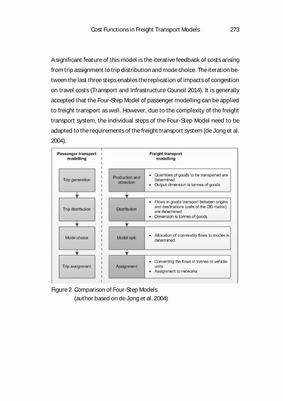
A significant feature of this model is the iterative feedback of costs arising
from trip assignment to trip distribution and mode choice. The iteration be-
tween the last three steps enables the replication of impacts of congestion
on travel costs (Transport and Infrastructure Council 2014). It is generally
accepted that the Four-Step Model of passenger modelling can be applied
to freight transport as well. However, due to the complexity of the freight
transport system, the individual steps of the Four-Step Model need to be
adapted to the requirements of the freight transport system (de Jong et al.
2004).
Figure 2 Comparison of Four-Step Models (author based on de Jong et al. 2004)

274 Katrin Brümmerstedt, Verena Flitsch and Carlos Jahn
A number of transformation modules are usually required (de Jong et al.
2004). An example for this is the converting of trade flows in monetary units
into physical flows in tons for the first step of the Four-Step Model. As trade
forms the basis for freight transport flows this is an inevitable step. For this
Tavasszy (2006) enhances the Four-Step Model by a fifth step ‘Trade’ after
the first step that includes the conversion of monetary units into tons. As
passenger transport does not relate back to monetary units no such trans-
lation has to be carried out in passenger modelling. The following elements
of freight transport models are necessary to carry out the illustrated model:
Table 1 Components of freight transport models (author)
Model Component Description
Demand model Different regional areas; Origin-destination data for different commodity groups as well as vehi-cle types
Network model Different networks for transport modes; Termi-nals for transfer between transport modes or the integration of logistics processes
Cost model Fixed and variable costs related to transport modes, vehicle types and commodity groups (or loading units)

Cost Functions in Freight Transport Models 275
The cost model is an essential component of freight transport models. In
most models the costs are linked to the network as part of a resistance
function. Freight transport models use costs in order to differentiate be-
tween different transport modes (and vehicle types) as well as commodity
groups (Müller et al. 2012). Costs occur at different stages of the transport
chain and can be found as resistors for the mode and route choice during
freight transport modelling. As part of common freight transport models
the transport mode, transport chain (incl. changes of transport modes) as
well as transport route are selected under the principle of minimization of
total costs of transport. The cost model is therefore a deterministic model
of cost minimization. Consequently, for freight transport models to be as
exact and realistic as possible, it is of special importance that the overall
costs of possible elements of logistical alternatives are calculated with suf-
ficient accuracy.
3 Macroscopic Freight Transport Models
Existing freight transport models do not only differ in terms of their inter-
national, national or regional perspective but also in relation to the data
used and their depth of aggregation, corresponding measurement varia-
bles used, or their scale of analysis named as aggregated or disaggregated.
Examples for macroscopic freight transport models are e.g. the Swedish
National Model System for Goods Transport (SAMGODS) and the Swiss Na-
tional Freight Transport Model (NGVM). Both models cover different
transport modes and commodity groups and consider all processes of tra-
ditional freight transport chains (transport, handling, storage). SAMGODS

276 Katrin Brümmerstedt, Verena Flitsch and Carlos Jahn
and NGVM are selected for further analysis because they can be considered
to belong to the best documented freight transport models. Table 2 com-
pares the two models with each other.
Table 2 Comparison of SAMGODS and the NGVM (author based on Vierth et al. 2009 and ARE 2011)
Criteria SAMGODS NGVM
Development period 2004-2009 2009-2011
Number of regions 290 in Sweden; 174 outside Sweden
2.945 in Switzerland; 156 outside Switzer-land
Level of aggregation Aggregated and Dis-aggregated
Aggregated and Dis-aggregated
Transport modes Road, rail, sea, air Road, rail
Logistics processes Transport, handling, storage
Transport, handling, storage
Number of freight categories 35 118
Software Own programming Visum
Cost Functions in Freight Transport Models 277
Both freight transport models are similar concerning the considered crite-
ria. Nevertheless, they differ from each other in their level of detail in terms
of the number of freight categories as well as the geographical coverage.
The level of aggregation of the NGVM is named as ‘Aggregated’ and ‘Dis-
aggregated’. Aggregated freight transport models do not take into consid-
eration flows between individual firms and logistics decisions but between
regions or zones. Disaggregated means, that logistics decisions (e.g. use of
consolidation and distribution centers, shipments sizes or loading units)
are included. For this, the NGVM includes so called logistics systems (e.g.
full truck load, pallets) (ARE 2011). Due to the fact that the information per
shipment is finally aggregated to origin-destination flows for the network
assignment the NGVM can be described as an aggregate-disaggregate-ag-
gregate (ADA) freight model system.
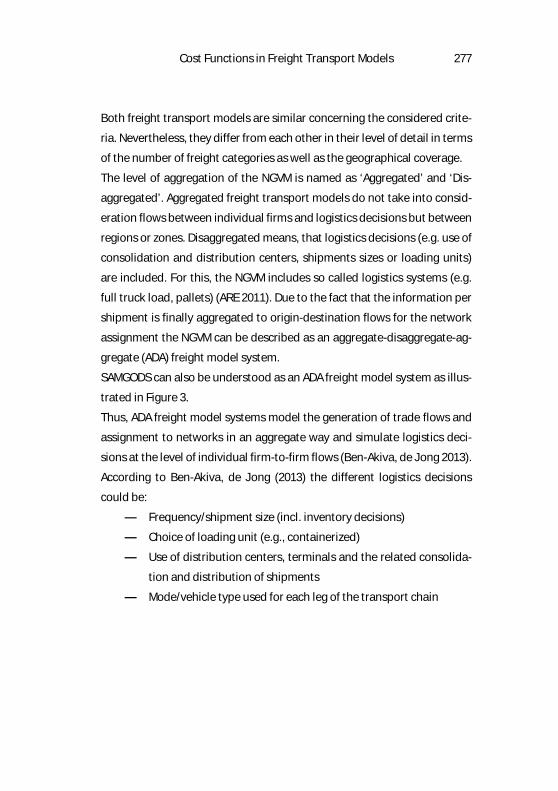
SAMGODS can also be understood as an ADA freight model system as illus-
trated in Figure 3.
Thus, ADA freight model systems model the generation of trade flows and
assignment to networks in an aggregate way and simulate logistics deci-
sions at the level of individual firm-to-firm flows (Ben-Akiva, de Jong 2013).
According to Ben-Akiva, de Jong (2013) the different logistics decisions
could be:
— Frequency/shipment size (incl. inventory decisions)
— Choice of loading unit (e.g., containerized)
— Use of distribution centers, terminals and the related consolida-
tion and distribution of shipments
— Mode/vehicle type used for each leg of the transport chain

278 Katrin Brümmerstedt, Verena Flitsch and Carlos Jahn
These logistics decisions are made with the overall objective of minimizing
total logistics costs. ADA freight model systems also have been developed
for Norway and Flanders and are currently under development in Denmark
and for the European Union (Ben-Akiva, de Jong 2013).
The development of a seaport hinterland model for the Port of Hamburg
will follow the underlying logic of the ADA freight model system.
Figure 3 Structure of SAMGODS model (author based on Karlsson et al. 2012)
4 Development of a Seaport Hinterland Model for the Port of Hamburg
The macroscopic freight transport model currently under development is
funded by the Ministry of Science and Research of the City of Hamburg. The
model follows the logic visualized in Figure 4.
In step 1, the transport networks as well as origin-destination matrices for
different commodity groups (according to value and density) are created in

Cost Functions in Freight Transport Models 279
the software environment Visum. This step comprises the first two steps of
the Four-Step Model as illustrated in Figure 2. The model includes road, rail
and inland waterway networks. These networks connect in total 380 de-
mand zones and 237 terminal zones across the whole of Europe. As part of
this first step, origin-destination, distance and time matrices between the
demand as well as terminal zones are calculated. These matrices form the
input for the second step.

280 Katrin Brümmerstedt, Verena Flitsch and Carlos Jahn
Figure 4 Traffic systems, modes, demand segments and demand matri-ces of the freight transport model under development (author)

Cost Functions in Freight Transport Models 281
The second step is carried out outside of the Visum environment by using a
Visual Basic for Applications (VBA) macro in Microsoft Excel. In this step the
least expensive transport chain for each origin-destination relation is cho-
sen by passing the following process:
1. Select the cheapest path between origin and destination without
transshipment.
2. Is there a cheaper path between origin and destination with one
transshipment move? If yes, select this path - If no, select path be-
tween origin and destination without transshipment.
3. Is there a cheaper path between origin and destination with two
transshipment moves? If yes, select this path - If no, select path
between origin and destination with one transshipment.
The total number of transshipments is limited to two transshipments and
distinction is made between different traffic systems (vehicle types). The
step complies with the third step of the Four-Step Model (modal split). The
result of this step is a certain path with a fixed modal split for each origin-
destination relation and commodity group.
The final step consists of the transfer of goods flows in tons into vehicle
flows and the assignment to the network. This step is again carried out in-
side the software Visum and complies with the fourth step of the Four-Step
Modal (assignment).
As described, especially the second step of the new model logic bases on
cost functions taking into consideration different transport modes, vehicle
types as well as commodity groups.

282 Katrin Brümmerstedt, Verena Flitsch and Carlos Jahn
5 Derivation of Cost Functions
In this section cost functions are derived and also applied to the use case
of the Port of Hamburg. For this, characteristics of the Port of Hamburg's
hinterland connections are presented first. Afterwards, cost functions im-
plemented in the ADA freight model system are analyzed and adapted to
the requirements of the model under development. Finally, the cost func-
tions are tested taking into account a transport chain significant for the
Port of Hamburg.
Total volumes handled in the Port of Hamburg amount to 145.7 million tons
in 2014. This means an overall increase of 4.8 percent compared to 2013.
Containers form about 70 percent of total throughput (9.7 million TEU
(Twenty-foot Equivalent Unit) in 2014, +5.1 percent compared to 2013 (HHM
2015a). According to the current German sea traffic forecast the relatively
high degree of containerization in the Port of Hamburg relates back to the
NST-2007 commodity group ‘not identifiable goods’, which amounts to 20
percent of all hinterland volumes. Relevant hinterland regions for this com-
modity group are especially Bavaria, the Czech Republic, Baden Württem-
berg, Bremen as well as North Rhine-Westphalia (MWP et al. 2014). How-
ever, the relevant hinterland regions for all freight categories handled in
the Port of Hamburg are different to that. Around 59.8 percent (5.8 million
TEU) of all containers handled in the Port of Hamburg are transported into
hinterland regions, most of them via the transport modes road (59.4 per-
cent, 3.4 million TEU) and rail (38.6 percent, 2.2 million TEU) (HHM 2015b).
Hinterland transport of containerized cargo via inland waterways forms a
negligible low part of all containerized hinterland transports (only 2.0 per-
cent).

Cost Functions in Freight Transport Models 283
Due to the Port of Hamburg's high degree of containerization and the sig-
nificance of the transport modes road and rail the development of cost
functions for transport chains in the hinterland of the Port of Hamburg will
focus on containerized cargo into relevant hinterland regions and road only
as well as rail-road transport chains.
ADA freight model systems include freight flows between zones or regions
as well as individual firms. The basic model for decision-making on the dis-
aggregated level (logistics decisions at the level of individual firm-to-firm
flows) is the minimization of total logistics costs. According to Ben-Akiva,
de Jong (2013) the disaggregated level consists of shipments of goods in
number of shipments, tons, ton-kilometers, vehicle-kilometers and vehi-
cle/vessels per year, by
𝑘𝑘, commodity type
𝑒𝑒, transport chain type (number of legs, mode and vehicle/vessel
type used for each leg, terminals used, loading unit used)
𝑎𝑎, sending firm (located in zone r)
𝑛𝑛, receiving firm (located in zone 𝑠𝑠)
𝑞𝑞, shipment size
As stated by Ben-Akiva, de Jong (2013) and Vierth et al. (2009) the total an-
nual logistics costs G of commodity k transported between firm m in pro-
duction zone r and firm n in consumption zone s of shipment size q with
transport chain l (including number of legs, modes, vehicle types, loading
units, transshipment locations) are:
𝐺𝐺𝑃𝑃𝑅𝑅𝑘𝑘𝑟𝑟𝐶𝐶𝑟𝑟𝑙𝑙 = 𝑃𝑃𝑘𝑘 + 𝐼𝐼𝑘𝑘𝑟𝑟 + 𝐾𝐾𝑘𝑘𝑟𝑟 + 𝑐𝑐𝑘𝑘𝑟𝑟 + 𝑇𝑇𝑃𝑃𝑅𝑅𝑘𝑘𝑟𝑟𝑙𝑙 + 𝑌𝑌𝑃𝑃𝑅𝑅𝑘𝑘𝑙𝑙 + 𝑍𝑍𝑃𝑃𝑅𝑅𝑘𝑘𝑟𝑟 (1)
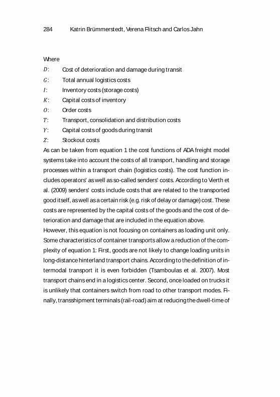
284 Katrin Brümmerstedt, Verena Flitsch and Carlos Jahn
Where
𝑃𝑃: Cost of deterioration and damage during transit
𝐺𝐺: Total annual logistics costs
𝐼𝐼: Inventory costs (storage costs)
𝐾𝐾: Capital costs of inventory
𝑐𝑐: Order costs
𝑇𝑇: Transport, consolidation and distribution costs
𝑌𝑌: Capital costs of goods during transit
𝑍𝑍: Stockout costs
As can be taken from equation 1 the cost functions of ADA freight model
systems take into account the costs of all transport, handling and storage
processes within a transport chain (logistics costs). The cost function in-
cludes operators' as well as so-called senders' costs. According to Vierth et
al. (2009) senders' costs include costs that are related to the transported
good itself, as well as a certain risk (e.g. risk of delay or damage) cost. These
costs are represented by the capital costs of the goods and the cost of de-
terioration and damage that are included in the equation above.
However, this equation is not focusing on containers as loading unit only.
Some characteristics of container transports allow a reduction of the com-
plexity of equation 1: First, goods are not likely to change loading units in
long-distance hinterland transport chains. According to the definition of in-
termodal transport it is even forbidden (Tsamboulas et al. 2007). Most
transport chains end in a logistics center. Second, once loaded on trucks it
is unlikely that containers switch from road to other transport modes. Fi-
nally, transshipment terminals (rail-road) aim at reducing the dwell-time of

Cost Functions in Freight Transport Models 285
containers in order not to lose too much time and to increase the competi-
tiveness of intermodal transport compared to road container transport.
A possible cost function representing containerized cargo is developed by
Jourquin, Tavasszy (2014). According to Jourquin, Tavasszy (2014) inter-
modal container transport is an alternative to road container transport
when the internal costs of the intermodal trip are competitive in compari-
son to the internal costs of trucking. Internal costs of moving a container
cover the sum of costs incurred by the various parties responsible for the
movement of the container (Black et al. 2003).
Following the authors argumentation the attractiveness of the intermodal
chain depends on the level of transshipment costs and on the length of the
pre- and post-haulages to and from the intermodal terminals. The authors
define the cost functions for road (Equation 2) and intermodal container
transport (Equation 3) as follows:
𝐶𝐶𝑔𝑔𝑃𝑃𝑃𝑃𝑉𝑉𝑟𝑟 = 𝑎𝑎𝑃𝑃𝑃𝑃𝑉𝑉𝑟𝑟 ∗ �ℎ𝑃𝑃𝑃𝑃𝑉𝑉𝑟𝑟𝑖𝑖𝑃𝑃𝑃𝑃𝑉𝑉𝑟𝑟
+ 𝑒𝑒𝑃𝑃𝑃𝑃𝑉𝑉𝑟𝑟� (2)
𝐶𝐶𝑔𝑔𝑃𝑃𝑉𝑉𝑖𝑖𝑙𝑙−𝑃𝑃𝑃𝑃𝑉𝑉𝑟𝑟 = 𝑎𝑎𝑃𝑃𝑉𝑉𝑖𝑖𝑙𝑙 �ℎ𝑃𝑃𝑉𝑉𝑖𝑖𝑙𝑙𝑖𝑖𝑃𝑃𝑉𝑉𝑖𝑖𝑙𝑙
+ 𝑒𝑒𝑃𝑃𝑉𝑉𝑖𝑖𝑙𝑙� + 𝐶𝐶𝑃𝑃𝑉𝑉𝑖𝑖𝑙𝑙−𝑃𝑃𝑃𝑃𝑉𝑉𝑟𝑟 �ℎ𝑃𝑃𝑃𝑃𝑉𝑉𝑟𝑟𝑖𝑖𝑃𝑃𝑃𝑃𝑉𝑉𝑟𝑟
+ 𝑅𝑅�
+ 𝑒𝑒𝑃𝑃𝑉𝑉𝑖𝑖𝑙𝑙−𝑃𝑃𝑃𝑃𝑉𝑉𝑟𝑟 + ℎ𝑃𝑃𝑉𝑉𝑖𝑖𝑙𝑙𝑒𝑒𝑃𝑃𝑉𝑉𝑖𝑖𝑙𝑙−𝑃𝑃𝑃𝑃𝑉𝑉𝑟𝑟 (3)
286 Katrin Brümmerstedt, Verena Flitsch and Carlos Jahn
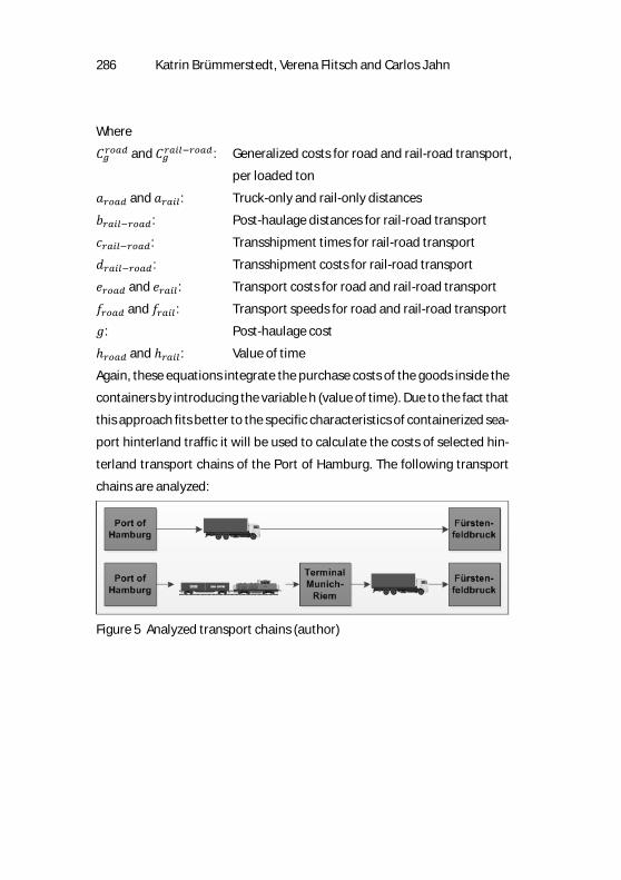
Where
𝐶𝐶𝑔𝑔𝑃𝑃𝑃𝑃𝑉𝑉𝑟𝑟 and 𝐶𝐶𝑔𝑔𝑃𝑃𝑉𝑉𝑖𝑖𝑙𝑙−𝑃𝑃𝑃𝑃𝑉𝑉𝑟𝑟: Generalized costs for road and rail-road transport,
per loaded ton
𝑎𝑎𝑃𝑃𝑃𝑃𝑉𝑉𝑟𝑟 and 𝑎𝑎𝑃𝑃𝑉𝑉𝑖𝑖𝑙𝑙: Truck-only and rail-only distances
𝐶𝐶𝑃𝑃𝑉𝑉𝑖𝑖𝑙𝑙−𝑃𝑃𝑃𝑃𝑉𝑉𝑟𝑟: Post-haulage distances for rail-road transport
𝑒𝑒𝑃𝑃𝑉𝑉𝑖𝑖𝑙𝑙−𝑃𝑃𝑃𝑃𝑉𝑉𝑟𝑟: Transshipment times for rail-road transport
𝑒𝑒𝑃𝑃𝑉𝑉𝑖𝑖𝑙𝑙−𝑃𝑃𝑃𝑃𝑉𝑉𝑟𝑟: Transshipment costs for rail-road transport
𝑒𝑒𝑃𝑃𝑃𝑃𝑉𝑉𝑟𝑟 and 𝑒𝑒𝑃𝑃𝑉𝑉𝑖𝑖𝑙𝑙: Transport costs for road and rail-road transport
𝑖𝑖𝑃𝑃𝑃𝑃𝑉𝑉𝑟𝑟 and 𝑖𝑖𝑃𝑃𝑉𝑉𝑖𝑖𝑙𝑙: Transport speeds for road and rail-road transport
𝑅𝑅: Post-haulage cost
ℎ𝑃𝑃𝑃𝑃𝑉𝑉𝑟𝑟 and ℎ𝑃𝑃𝑉𝑉𝑖𝑖𝑙𝑙: Value of time
Again, these equations integrate the purchase costs of the goods inside the
containers by introducing the variable h (value of time). Due to the fact that
this approach fits better to the specific characteristics of containerized sea-
port hinterland traffic it will be used to calculate the costs of selected hin-
terland transport chains of the Port of Hamburg. The following transport
chains are analyzed:
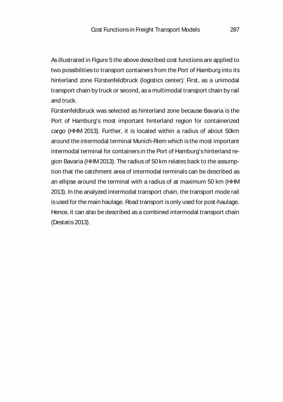
Figure 5 Analyzed transport chains (author)
Cost Functions in Freight Transport Models 287
As illustrated in Figure 5 the above described cost functions are applied to
two possibilities to transport containers from the Port of Hamburg into its
hinterland zone Fürstenfeldbruck (logistics center): First, as a unimodal
transport chain by truck or second, as a multimodal transport chain by rail
and truck.
Fürstenfeldbruck was selected as hinterland zone because Bavaria is the
Port of Hamburg's most important hinterland region for containerized
cargo (HHM 2013). Further, it is located within a radius of about 50km
around the intermodal terminal Munich-Riem which is the most important
intermodal terminal for containers in the Port of Hamburg's hinterland re-
gion Bavaria (HHM 2013). The radius of 50 km relates back to the assump-
tion that the catchment area of intermodal terminals can be described as
an ellipse around the terminal with a radius of at maximum 50 km (HHM
2013). In the analyzed intermodal transport chain, the transport mode rail
is used for the main haulage. Road transport is only used for post-haulage.
Hence, it can also be described as a combined intermodal transport chain
(Destatis 2013).
288 Katrin Brümmerstedt, Verena Flitsch and Carlos Jahn
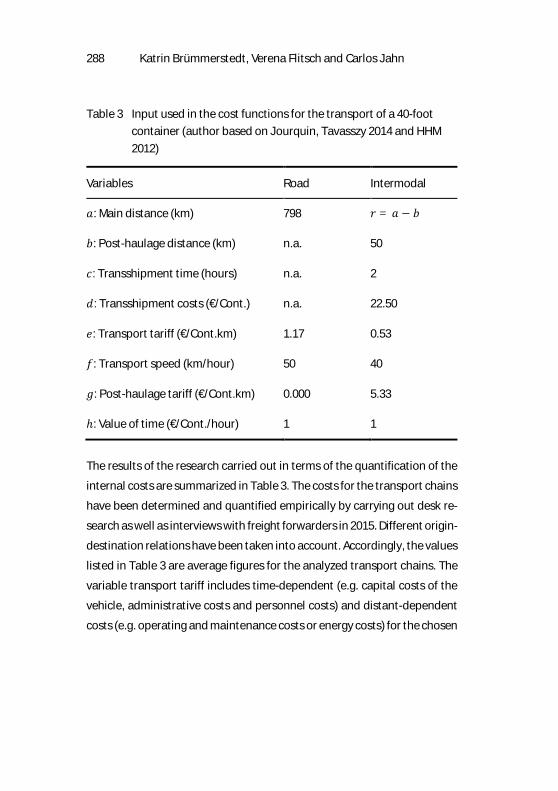
Table 3 Input used in the cost functions for the transport of a 40-foot container (author based on Jourquin, Tavasszy 2014 and HHM 2012)
Variables Road Intermodal
𝑎𝑎: Main distance (km) 798 𝑟𝑟 = 𝑎𝑎 − 𝐶𝐶
𝐶𝐶: Post-haulage distance (km) n.a. 50
𝑒𝑒: Transshipment time (hours) n.a. 2
𝑒𝑒: Transshipment costs (€/Cont.) n.a. 22.50
𝑒𝑒: Transport tariff (€/Cont.km) 1.17 0.53
𝑖𝑖: Transport speed (km/hour) 50 40
𝑅𝑅: Post-haulage tariff (€/Cont.km) 0.000 5.33
ℎ: Value of time (€/Cont./hour) 1 1
The results of the research carried out in terms of the quantification of the
internal costs are summarized in Table 3. The costs for the transport chains
have been determined and quantified empirically by carrying out desk re-
search as well as interviews with freight forwarders in 2015. Different origin-
destination relations have been taken into account. Accordingly, the values
listed in Table 3 are average figures for the analyzed transport chains. The
variable transport tariff includes time-dependent (e.g. capital costs of the
vehicle, administrative costs and personnel costs) and distant-dependent
costs (e.g. operating and maintenance costs or energy costs) for the chosen

Cost Functions in Freight Transport Models 289
transport modes. Using the input data the costs for the different transport
chains are
— 949.62 €/40-foot container for road only container transport and
— 707.14 €/40-foot container for intermodal container transport.
The transport costs of a 40-foot container with an average load capacity of
30.40 tons from Hamburg to the logistics center in Fürstenfeldbrück
amount to 0.039 €/t.km for the road only transport and 0.029 €/tkm for the
intermodal transport. The intermodal option turns out to be significantly
cheaper than the road only alternative. This corresponds to observations
made by Ricci (2003) or Black et al. (2003).
6 Discussion and Further Research
The chosen transport tariff for road transport is based on the assumption,
that the average cost of movement by road amounts to 1.19 €/km for a 40-
foot container. This value corresponds to the figures published in Black et
al. (2003). As reported by them the value for moving a 40-foot container in
Germany is 1.14 €/km. According to HHM (2012) the cost of moving a 40-
foot container between Hamburg and Bavaria amounts to 1.17 €/km.
For intermodal transport it is assumed that the average cost for moving a
40-foot container amounts to 0.89 €/km. Again, this figure lies within a
range that can be found in different studies. Within the project Hafen Ham-
burg 62+ systematic comparisons of costs have been carried out for differ-
ent transport chains between Bavaria and Hamburg. Within the project, rail
haul unit costs of roughly 0.79 €/km per 40-foot container were identified
for container transports between Hamburg and Munich (HHM 2012).
290 Katrin Brümmerstedt, Verena Flitsch and Carlos Jahn
Following this argumentation, the achieved results are in conformity with
the current state of practice. However, several aspects have been neglected
so far:
1. Different vehicle types. The calculation does just take into consid-
eration one vehicle type (long-distance truck). But, operational
costs can be different for different vehicle types.
2. Different commodity groups with different logistics backgrounds.
The variable 'value of time' has not been quantified so far. Conse-
quently, the purchaser's costs of the content of containers are not
integrated. Neither are the specific requirements of different
commodity groups, e.g. urgency of transport.
3. Different network types. The cost function calculates with aver-
age speeds and considers only one possible route.
4. Capacity restrictions. The interdependencies of different
transport chains as well as capacity restrictions have been ne-
glected so far. The attractiveness of a transport chain is depend-
ent on the degree of utilization. The more containers are assigned
to a transport chain (and route) the less attractive it will be be-
cause of an increasing probability of congestion.
Consequently, the described cost function can only be seen as a first ap-
proach towards the development of a cost function usable in the model un-
der development.
Cost Functions in Freight Transport Models 291
7 Conclusion
Freight transport models are a useful tool for estimating the expected im-
pacts of policy measures and are a necessary input for the justification of
infrastructure measures. Based on cost functions transport demand is as-
signed to the transport network and different transport modes.
When intermodal transport competes with road transport, trucks are used
in two different ways: Either they are used as a substitute for or as a com-
plement for the rail. Nevertheless, for the analyzed Origin-Destination rela-
tion (Hamburg-Munich) the intermodal option turns out to be significantly
cheaper than the road only alternative (707.14 €/Cont. for intermodal con-
tainer transport compared to 949.62 €/Cont. for road only container
transport).
The described cost function can be seen as a first approach to calculate the
total costs of the Port of Hamburg's containerized hinterland transport
chains. It needs to be extended by a quality variable that integrates the in-
terdependencies of different transport chains as well as the probability of
congestion in order to describe the transport market in a more realistic
way. The sensitivity to cost changes or situational responses because of in-
terdependencies as well as the differentiation between goods with differ-
ent logistics backgrounds are challenges that need to be integrated into
cost functions of an appropriate seaport hinterland model for the Port of
Hamburg.

292 Katrin Brümmerstedt, Verena Flitsch and Carlos Jahn
References
ARE Bundesamt für Raumentwicklung (2011): Nationales Güter-verkehrsmodell des UVEK. Basismodell 2005: Modellbeschrieb und Validierung. Eidg. Departement für Umwelt, Verkehr, Energie und Kommunikation (UVEK). Zürich.
Ben-Akiva, M.; de Jong, G. (2013): The Aggregate-Disaggregate-Aggregate (ADA) Freight Model System. In M. Ben-Akiva, E. van de Voorde, H. Meersman (Eds.): Freight Transport Modelling. 1st ed. Bingley, United Kingdom: Emerald, pp. 69–90.
Ben-Akiva, M.; Meersman, H.; van de Voorde, E. (2013): Recent Developments in Freight Transport Modelling. In M. Ben-Akiva, E. van de Voorde, H. Meersman (Eds.): Freight Transport Modelling. 1st ed. Bingley, United Kingdom: Emerald, pp. 1–13.
Black, I.; Seaton, R.; Ricci, A.; Enei, R.; Vaghi, C.; Schmid, S.; Bühler, G. (2003): RE-CORDIT Final Report: Actions to Promote Intermodal transport. Available online at http://www.transport-re-search.info/Upload/Docu-ments/200607/20060727_155159_96220_RECORDIT_Final_Re-port.pdf&bvm=bv.96339352,d.bGQ&cad=rja, updated on 26/05/2003, checked on 3/03/2015.
de Jong, G.; Gunn, H.F; Walker, W. (2004): National and international freight transport models: overview and ideas for further development. In Transport Re-views. 24 (1), pp. 103–124.
Destatis Statistisches Bundesamt (2013): Kombinierter Verkehr - Fachserie 8 Reihe 1.3. Wiesbaden.
HHM Hafen Hamburg Marketing e.V. (2012): Wege zur Stärkung der Bahn im Contai-ner-Hinterlandverkehr zwischen dem Hafen Hamburg und dem Freistaat Bay-ern. Stärken, Chancen, Entwicklungspotenziale. Ergebnisse eines bayerisch-hamburgischen Kooperationsprojektes.
HHM Hafen Hamburg Marketing e.V. (2013): Kooperationsprojekt Hafen Hamburg 62+. Vertraulicher Abschlussbericht.

Cost Functions in Freight Transport Models 293
HHM Port of Hamburg Marketing e.V. (2015a): Cargo Handling 2014 in million tons. Available online at http://www.hafen-hamburg.de/de/statistiken, checked on 17/06/2015.
HHM Port of Hamburg Marketing e.V. (2015b): Modal-Split in Container Traffic. Available online at http://www.hafen-hamburg.de/en/statistics/modalsplit, checked on 17/06/2015.
Jourquin, B.; Tavasszy, L. and Duan L. (2014): On the generalized cost - demand elasticity of intermodal container transport. In Europe-an Journal of Transport and Infrastructure Research 14 (4), pp. 362–374.
Karafa, J. (2010): State-of-the-Art in Freight Modeling. Undergraduate Paper ITE Dis-trict No. 5. The University of Memphis.
Karlsson, R.; Vierth, I.; Johansson, M. (2012): An outline for a validation database for SAMGODS. vti. Linköping.
Merk, O. (2013): The Competitiveness of Global Port-Cities: Synthesis Report. Organ-isation for Economic Co-operation and Development (OECD), checked on 15/06/2015.
Müller, Stephan; Wolfermann, Axel; Huber, Stefan (2012): A Nation-wide Macro-scopic Freight Traffic Model. EWGT 2012 - 15th meeting of the EURO Working Group on Transportation. In Procedia - Social and Behavioral Sciences 54, pp. 221–230.
MWP; IHS; UNICONSULT; Fraunhofer CML (2014): Verkehrsver-flechtungsprognose 2030 sowie Netzumlegung auf die Verkehrsträ-ger; Los 2 (Seeverkehrsprog-nose). Forschungsbericht FE-Nr. 96.980-2011. Im Auftrag des Bundesministeri-ums für Verkehr und digitale Infrastruktur.
OECD Organisation for Economic Co-operation and Development (2014): Statistics Brief July 2014. Global Trade and Transport. Available online at http://www.eea.europa.eu/publications/european-union-greenhouse-gas-in-ventory-2014/greenhouse-gas-inventory-2014-full.pdf, updated on 17/07/2014, checked on 9/06/2015.
Ricci, A. (2003): Pricing of Intermodal Transport. Lessons Learned from RECORDIT. In European Journal of Transport and Infrastructure Research 3 (4), pp. 351–370.
294 Katrin Brümmerstedt, Verena Flitsch and Carlos Jahn
Tavasszy, L. (2006): Freight Modelling - An overview of international experiences. TRB Conference on Freight Demand Modelling: Tools for Public Sector Decision Making. Washington DC, 25/09/2006.
Tavasszy, Lorant; Jong, Gerard de (Eds.) (2014): Modelling freight transport. First edition. London; Waltham: Elsevier Inc.
Transport and Infrastructure Council (2014): 2014 National Guidelines for TRansport System Management in Australia. Passenger Transport Modelling [T1].
Tsamboulas, Dimitrios; Vrenken, Huub; Lekka, Anna-Maria (2007): Assessment of a transport policy potential for intermodal mode shift on a European scale. In Transportation Research Part A: Policy and Practice 41 (8), pp. 715–733.
Vierth, I.; Lord, N.; Mc Daniel, J. (2009): Representation of the Swedish transport and logistics system. (Logistics Model Version 2.00). vti. Linköping (VTI notat 17A-2009). Available online at http://www.vti.se/en/publications/representation-of-the-swedish-transport-and-logistics-system-logistics-model-version-200/, up-dated on 9/06/2009, checked on 19/03/2015.