cost efficiency of microfinance institutions in peru: a stochastic frontier approach

This article was downloaded by: [McGill University Library]On: 15 October 2014, At: 02:36Publisher: RoutledgeInforma Ltd Registered in England and Wales Registered Number: 1072954 Registered office: Mortimer House,37-41 Mortimer Street, London W1T 3JH, UK

Latin American Business ReviewPublication details, including instructions for authors and subscription information:http://www.tandfonline.com/loi/wlab20

Cost Efficiency of Microfinance Institutions in Peru: AStochastic Frontier ApproachJorge R. Gregoire a & Oswaldo Ramírez Tuya ba Faculty of Economic and Administrative Sciences , Universidad de Chile , Santiago, Chile E-mail:b Department of Economics , Universidad Nacional de Ancash , Santiago Antúnez de Mayolo,Peru E-mail:Published online: 12 Oct 2008.

To cite this article: Jorge R. Gregoire & Oswaldo Ramírez Tuya (2006) Cost Efficiency of Microfinance Institutions in Peru: AStochastic Frontier Approach, Latin American Business Review, 7:2, 41-70

To link to this article: http://dx.doi.org/10.1300/J140v07n02_03

PLEASE SCROLL DOWN FOR ARTICLE

Taylor & Francis makes every effort to ensure the accuracy of all the information (the “Content”) containedin the publications on our platform. However, Taylor & Francis, our agents, and our licensors make norepresentations or warranties whatsoever as to the accuracy, completeness, or suitability for any purpose of theContent. Any opinions and views expressed in this publication are the opinions and views of the authors, andare not the views of or endorsed by Taylor & Francis. The accuracy of the Content should not be relied upon andshould be independently verified with primary sources of information. Taylor and Francis shall not be liable forany losses, actions, claims, proceedings, demands, costs, expenses, damages, and other liabilities whatsoeveror howsoever caused arising directly or indirectly in connection with, in relation to or arising out of the use ofthe Content.

This article may be used for research, teaching, and private study purposes. Any substantial or systematicreproduction, redistribution, reselling, loan, sub-licensing, systematic supply, or distribution in anyform to anyone is expressly forbidden. Terms & Conditions of access and use can be found at http://www.tandfonline.com/page/terms-and-conditions

http://www.tandfonline.com/loi/wlab20

http://dx.doi.org/10.1300/J140v07n02_03

http://www.tandfonline.com/page/terms-and-conditions

http://www.tandfonline.com/page/terms-and-conditions

Cost Efficiencyof Microfinance Institutions in Peru:

A Stochastic Frontier Approach

Jorge R. GregoireOswaldo Ramírez Tuya

ABSTRACT. This paper analyzes the efficiency of Microfinance Insti-tutions (MFIs) in Peru between 1999 and 2003 by estimating a stochasticcost frontier. The main findings show that MFIs with the largest assetstend to post the highest efficiency levels, and that MFIs operating in lessconcentrated markets tend to be more efficient. Thus, the cost efficiencyof MFIs is affected by average loan size, proportion of net assets, finan-cial sufficiency, financial leverage, business experience and proportionof farm loans.RESUMEN. Este trabajo analiza la eficiencia de las InstitucionesMicrofinancieras (IMF) en el Perú en el periodo 1999-2003 mediantela estimación de una frontera estocástica de costos. Los principalesresultados muestran que las IMF con mayor tamaño de activos tienden amostrar mayores niveles de eficiencia y que las IMF operando enmercados menos concentrados tienden a ser más eficientes. Asimismo,afectan la eficiencia en costos de las IMF el tamaño promedio de loscréditos, la proporción de activos líquidos, la suficiencia financiera, elleverage financiero, la experiencia de negocios y la proporción de loscréditos agrícolas.RESUMO. Este artigo analisa a eficiência de Instituições de Micro-finanças (IDFs) no Peru entre 1999 e 2003, estimando uma fronteira

Jorge R. Gregoire is Professor, Faculty of Economic and Administrative Sciences,Universidad de Chile, Santiago, Chile (E-mail: [email protected]).

Oswaldo Ramírez Tuya is Assistant Professor, Department of Economics,Universidad Nacional de Ancash, Santiago Antúnez de Mayolo, Peru (E-mail:[email protected]).

Latin American Business Review, Vol. 7(2) 2006Available online at http://labr.haworthpress.com

© 2006 by The Haworth Press, Inc. All rights reserved.doi: 10.1300/J140v07n02_03 41

Dow

nloa

ded

by [

McG

ill U

nive

rsity

Lib

rary

] at

02:

36 1

5 O

ctob

er 2

014

estocástica de custo. As principais descobertas mostram que IDFs comos maiores ativos tendem a anunciar os maiores níveis de eficiência, eque IDFs operando em mercados menos concentrados tendem a ser maiseficientes. Desse modo, a eficiência de custos de IDFs é afetada pelotamanho médio do empréstimo, proporção de ativos líquidos, suficiênciafinanceira, alavancagem financeira, experiência no negócio e proporção definanciamentos agrícolas. doi:10.1300/J140v07n02_03 [Article copies avail-able for a fee from The Haworth Document Delivery Service: 1-800- HAWORTH.E-mail address: <[email protected]> Website: <http://www.HaworthPress.com> © 2006 by The Haworth Press, Inc. All rights reserved.]

KEYWORDS. Costs efficiency, stochastic frontier, microfinance insti-tutions

1. INTRODUCTION

The financial reform process implemented in Peru during the 1990screated a context that favored the development of microfinance,1 foster-ing the establishment of a series of non-bank financial institutions knownas Microfinance Institutions (MFIs). More specifically, due to firm con-straints imposed by traditional banks on financing small and micro enter-prises (SMEs2), which to a large extent reflect a lack of financialtechnology appropriate for this segment (Portocarrero, 2000), these insti-tutions flourished by channeling funds into this huge and dynamic sectorof the economy.3 The institutions comprising the microfinance segmentin Peru may be clustered into two categories by their institutional charac-teristics (Portocarrero, 2000). On the one hand are banks and financialentities specialized in servicing low-income sectors, such as Banco delTrabajo, Mibanco and Financiera Solución, which are authorized tocarry out multiple transactions, and which act nationwide, while on theother hand, non-bank Microfinance Institutions such as Municipal Sav-ings and Credit Unions (CMACs−Cajas Municipales de Ahorro y Cré-dito),4 Rural Savings and Credit Unions (CRACs−Cajas Rurales deAhorro y Crédito) and Small and Middle Size Enterprise DevelopmentEntities (EDPYME−Entidades de Desarrollo de la Pequeña y Micro-empresa) are authorized to perform a limited set of transactions, and mostof them generally operate on a regional scale. Each of them emerged withinspecific contexts and consequently each of them has individual character-istics that influence their behavior and performance5 (see Appendix 1).

42 LATIN AMERICAN BUSINESS REVIEW

Dow

nloa

ded

by [

McG

ill U

nive

rsity

Lib

rary

] at

02:

36 1

5 O

ctob

er 2

014

Due to the importance of micro-financing for fostering the develop-ment of SMEs, it is important to analyze the cost efficiency of MFIs andthe factors that determine their performance. In order to carry out thissurvey, a stochastic cost frontier model was used, proposed by Batteseand Coelli (1995). This model allows the inefficiency of each institutionto change over time, and in turn may also be the function of some vari-ables whose parameters are estimated simultaneously with the stochas-tic frontier. As potential factors determining inefficiency, two sets ofvariables are explored: those specified for each institution and those thatreflect the context in which MFIs develop.

This study is arranged as follows: Section 2 presents the theoreticalframework and reviews a few empirical efficiency studies. Section 3explains the methodology and the sample, Section 4 outlines the empiri-cal findings, and Section 5 presents the conclusions.

2. THEORETICAL FRAMEWORK

2.1 Cost Efficiency

As indicated by Berger and Mester (1997), cost efficiency showshow close corporate costs are to the costs of a company located on thefrontier, producing the same output under the same conditions. This isderived from a cost function, as shown below:

C C w y z v uC C= ( , , , , ) (1)

where C measures the variable costs, w is the variable input price vector,y is the variable quantities output vector, z shows the fixed netput quan-tities (input or output), vC is the normal random error and uC denotes aninefficiency factor (technical and allocative), which may increase costsabove the best practice level. Assuming that the random termination andinefficiency are multiplicatively separable from the rest of the cost func-tion arguments, this may be represented in natural logarithms, such as:

lnC f w y z v uC C= + +( , , ) ln ln (2)

where f denotes some functional form and the termination is treated as acompound error termination. The cost efficiency is defined as the quo-tient between the minimum cost that can be obtained for a specific out-put vector if company b were as efficient as a company in the sample

Jorge R. Gregoire and Oswaldo Ramírez Tuya 43

Dow

nloa

ded

by [

McG

ill U

nive

rsity

Lib

rary

] at

02:

36 1

5 O

ctob

er 2

014

located on the frontier, and the effective cost of company b, adjusted byrandom error facing the same exogenous variables (w,y,z), namely:

ECC

C

f w y z v

fb

b

b b bC= =

�

�

exp[ �( , , )] * exp[ � ]

exp[ �

min minln

( , , )] * exp[ln � ] * exp[ln � ]w y z v ub b bC C

b

(3)

EC ub C= −exp[ � ]

The cost efficiency (CE) indicator may be viewed as a proportion ofcosts or funds used efficiently. For example, a company with CE = 0.70is 70% efficient or, in other words, it may produce the same output vec-tor with savings of 30% (1−CE) of its costs, compared to the companylocated on the frontier under the same conditions. The efficiency indica-tor range is [0,1], equal to 1 for a company that is 100% efficient.

2.2 Efficiency Measurement Methods

The methodologies for measuring efficiency differ basically throughthe way in which the efficient frontier is determined, and the distribu-tive assumptions imposed on the random error and inefficiency. Non-parametric techniques do not take on any explicit functional form of theefficient frontier; the most widely-used technique is called Data Envel-opment Analysis (DEA). Berger and Mester (1997) and Berger andHumphrey (1997) explain that these methods generally do not take in-put prices into account, and consequently measure only technical ineffi-ciency, which is why they cannot compare firms tending to specialize indifferent inputs or outputs. Second, non-parametric techniques do notconsider the possibility of random errors in the efficiency measurement.On the other hand, parametric methods assume that the efficient frontierhas a specific functional form (Cobb-Douglas, Translog or FourierFlexible) and differ in the way that they separate inefficiency from therandom error. There are three main parametric approaches: the Stochas-tic Frontier Approach (SFA), the Distribution-Free Approach (DFA)and the Thick Frontier Approach (TFA). The SFA consists of estimat-ing a function where the explicative variables are the prices and thequantities of the inputs and outputs,6 in addition to other variables thatdescribe the context surrounding the companies. The regression residu-als reflect differences in efficiency among the companies and the possi-ble noise affecting their performance. Therefore, in order to obtain an


Dow

nloa

ded

by [

McG

ill U

nive

rsity

Lib

rary

] at

02:

36 1

5 O

ctob

er 2

014

inefficiency measurement that does not depend on stochastic shocks, itis necessary to break down the error obtained in these two elements. It isassumed that inefficiencies follow an asymmetrical distribution (half-normal, truncated normal), due to the fact that these cannot be negative,while random errors follow a symmetrical distribution (standard normal).The inefficiency measurement for any company is obtained as the esti-mated mean average of the conditional distribution of the inefficiencytermination, due to the observation of the compound termination error.7

DFA is a special SFA that may be estimated through a data base andthe unwinding of previous distributional assumptions (see Berger, 1993).Finally, TFA specifies the same functional form for the frontier as SFAand DFA, but proposes to divide the sample into different groups by his-toric performance in order to separate the “efficient” companies fromtheir “inefficient” counterparts. Having completed this step, a cost fron-tier is then estimated for each group.

In a compendium of 130 efficiency frontier studies of financial insti-tutions carried out worldwide, Berger and Humphrey (1997) found that116 were written or published between 1992 and 1997, with 66 of themfocused on the USA. These studies differed in the concept of efficiencyused, as well as the selected measurement technique, sample period andsize. Berger and Mester (1997) found that despite the variety of ap-proaches used, the cost efficiency of the banking industry in the USAhovers around 80%, with the benefits efficiency at around 54%.

Maudos and Pastor (2000) estimate a stochastic cost frontier for1,852 companies in fourteen countries belonging to the European Un-ion, using a DFA parametric approach and a translog specification forthe period 1992-1997. This study finds that the average cost efficiencyis 93%, and the average benefits efficiency is 64%. Maudos (2001) usesfrontier estimation techniques to study the Spanish financial system inthe period 1986-1995, with the efficiency average of the banks and sav-ings institutions reaching 66.7% and 84.2%, respectively.

In Latin America, studies intending to measure the efficiency of banksare more recent and are still scarce. For the Chilean banking industry,Fuentes and Vergara (2003) used the SFA method and a translog speci-fication for the period 1990-2000, finding that the cost efficiency aver-ages out at 91%, dropping over time, and the average benefit efficiencyreaches 75%, constant over time. The authors find that inefficiency isaffected positively by the type of ownership (local, public stock banksare the most efficient), while market concentration is affected nega-tively by size, financial risk and credit risk. Additionally, economic ac-tivity has negative effects on inefficiency.


Dow

nloa

ded

by [

McG

ill U

nive

rsity

Lib

rary

] at

02:

36 1

5 O

ctob

er 2

014

For the Colombian banking industry, also using the SFA method anda translog specification, Janna (2003) found an average cost efficiencyof 34% over the period 1992-2002, rising over time to 63% in 2002.Looking at the potential determining factors for this inefficiency, theauthor also found evidence that this is negatively related to the type ofownership (foreign banks are less inefficient than state-owned and pri-vate domestic banks), the type of business and the return on assets; it ispositively related to portfolio quality, regulations (heavier financialconstraints mean more inefficiency) and market concentration. Theeconomic cycle is not significant in explaining inefficiency.

For Peru, León (2003) estimates cost frontiers using the SFA, DFAand DEA techniques to measure the efficiency of CMACs for the period1994-1999. He notes that, using the SFA technique, efficiency risesfrom 69% to 91% between the two sub-periods, while efficiency dropsfrom 52% to 44% using the DEA technique. Thus, he explores the po-tential variables explaining this efficiency, which describe corporatecharacteristics, finding evidence that this is positively related to loca-tion, employee productivity and asset value, and is negatively related tosize (small and medium CMACs are more efficient) and age. He alsofinds that corporate governance, deposit-loan ratio, exposure to risk, fi-nancial sufficiency and return on assets are important variables for ex-plaining efficiency.

3. METHODOLOGY

3.1 Model Specification

A stochastic cost frontier model is used, which allows the observedcost of MFIs to deviate from the efficient frontier due to either randomevents and/or possible inefficiencies. According to Battese and Coelli(1995), a model is used that allows alterations in inefficiency over timeand, in turn, allows inefficiency itself to be a function of certain explica-tive variables whose parameters are estimated simultaneously with thestochastic frontier. This can explain the inefficiency of companiesthrough exogenous variables proper for each company or industry, andwhich do not form part of the cost frontier’s functional form.

When a set of analyzed data covers a cluster of companies over aperiod of time, the model may be written as:


Dow

nloa

ded

by [

McG

ill U

nive

rsity

Lib

rary

] at

02:

36 1

5 O

ctob

er 2

014

ln ( )C f x v uit it it it= + +b (4)

where:

• Cit is the corporate production cost i (i = 1, 2, …, N) over period oftime t (t = 1, 2, …, T).

• f is the functional form• xit is a vector (1xk) of input prices, product quantities and fixed

netputs of company i over period of time t.• b is the vector (kx1) of unknown parameters to be estimated.• vit are random variables that are assumed to be iid N v( , )0 2s and in-

dependent of uit.• uit are non-negative random variables that cover the technical inef-

ficiency in cost and are assumed to be distributed independently,truncated at zero of the distribution N Zit u( , )δ σ 2 where:

• Zit is a vector (1xm) of explicative variables associated with techni-cal inefficiency in the cost of companies over time, and

• d is a vector (mx1) of unknown coefficients to be estimated.

From the above, it appears that the effect of technical inefficiency uitmay be specified as follows:

u Zit it it= +d e (5)

where a random variable eit follows a normal truncated distribution witha zero average and a s e

2 variant. The truncation point is determined

at −Zitd, such that uit will always be greater than or equal to zero, that is,e dit itZ≥ − .

The joint estimation for the parameters for the stochastic frontiermodel and the technical inefficiency effects model is carried out on thegreatest likelihood basis.

3.2 Functional Form

The functional form used to estimate the frontier cost function is thetranslog, similar to Berger and Mester (1997), Fuentes and Vergara(2003), Janna (2003), Maudos (1996) and others.8 For a cost functionwith k input, m products and r fixed netputs, the translog cost functionadopts the following specification:


Dow

nloa

ded

by [

McG

ill U

nive

rsity

Lib

rary

] at

02:

36 1

5 O

ctob

er 2

014

ln ln ln lninput output

C w y zk kk

m mm

r r= + + += =∑ ∑a b a j0 ( ) ( ) ( )

r

kkl

lk

m

w wl

=

= = =

∑

∑ ∑+ +

netput

input input ou

ln ln1

2

1

2b ( ) ( )

tput output

netput n

ln ln∑ ∑

∑=

= =+

a

j

mn m ny y

n

rrs

s

( ) ( )( )6

1

2 etput input output

ln ln ln ln∑ ∑ ∑+= =

( ) ( ) ( ) (z z w yr sk

kmm

k mh )

+= = = =∑ ∑ ∑

kkr

sk r

mmr

r

w zinput netput output n

ln( )ln( )+r tetput

ln( )ln( )+∑ +y z v um r

In the literature, constraints are typically imposed on the homogene-ity of this function in order to ensure that it is grade one, such as:

b b h r tk kl km kr mr= = = = =∑∑ ∑∑ ∑∑∑ ∑∑1 0 0 0 0, , , , (7)

These constraints may be imposed through estimating a model wherethe cost and the price of the k-1 inputs are normalized by the price of thek-nth input. Similarly, through symmetry, it should be noted that:

b b a a j jkl kl mnl nm rs srk l m n y r s= ≠ = ≠ = ≠si si si, , ,(8)

3.3 Variables and Sample Used

3.3.1 Sample

In order to calculate the stochastic cost frontier and the inefficiencyeffect model, a data base was built with monthly information from No-vember 1999 through September 2003. The data were provided by SBS.The study includes all the MFIs in existence during each period: 3 MFbanks, 13 CMACs, 12 CRACs and the EDPYMEs, which rose from 7 to14 during the period covered by the study, which is why an incompletedata panel was used, with 1,864 observations.

3.3.2 Cost Function Variables

The dependent variable is the total cost. A thorny issue faced by allstudies analyzing the technology underlying the production function ofa financial intermediary is the identification and measurement of out-put, because there is no consensus on the treatment of this variable. This


Dow

nloa

ded

by [

McG

ill U

nive

rsity

Lib

rary

] at

02:

36 1

5 O

ctob

er 2

014

study uses the financial intermediation approach, so that the only outputconsists of direct loans.

Work and physical capital represent the inputs required for the produc-tion of the financial output; however, treating the deposits as input ismore open to discussion. Nevertheless, if only Capital and Work are con-sidered, the measured efficiency will refer only to the operating costs. Asa financial is an important part of the total cost, the cost concept appropri-ate for measuring the efficiency of a financial entity consists of the totalcosts, which include the operating costs and the financial costs. Thismeans that the financial input and the constraints imposed on theEDPYMEs must be estimated in terms of obtaining deposits from thepublic, and requiring them to post all portions of the liabilities giving riseto financial costs under the generic name of “lendable funds,” which in-clude deposits from the public, deposits from the financial system and in-ternational entities, interbank funds as well as financial obligations anddebt.

It may be observed that “outsourced services” account for an importantportion of the cost structure of the FMIs, but since the items covered by thisheading are very heterogeneous and hard to identify with a physical unitthat allows their unit costs to be estimated, they have been included in thisstudy as a fixed netput. According to Berger and Mester (1997) andMaudos and Pastor (2000), this is included in the fixed assets cost function.


TABLE 1. Definition of the Cost Function Variables

Variable Definition

Total cost (C) Includes operating costs (labor costs, physical capital andother overhead) and financial costs.

Direct loans (y1) Includes loans in effect plus refinanced and restructuredloans, plus the overdue portfolio.

Lendable funds price (w1) Calculated by dividing the lendable fund costs by the totallendable fund, which includes liabilities to the public, financialsystem and international entity deposits, inter-bank funds,debts and financial obligations.

Labor input price (w2) Calculated by dividing personnel costs by the number ofworkers.

Physical capital price (w3) Calculated by dividing the physical capital costs (depreciationand amortization) by the fixed assets, net of depreciation.

Other administrativeexpenses (z1)

Includes director’s allowances, outsourced services, taxesand fees.

Capital and reserves (z2) Includes paid-in capital, legal reserves and stock subscriptionpremiums.

Dow

nloa

ded

by [

McG

ill U

nive

rsity

Lib

rary

] at

02:

36 1

5 O

ctob

er 2

014

3.3.3 Factors Determining Efficiency

In terms of the potential factors determining inefficiency, two sets ofvariables were used. One consisted of variables specific to each MFI,which describe its characteristics and which relate to the administrationof its financial resources, which may have direct or indirect effects onits functioning, including size, ownership and governance, experience,business, financial management and risk. The other covers the businesscontext in order to reflect the absolute level of inefficiency of the FMIsinstead of the differences among them, including market concentrationand economic cycles.

Table 2 summarizes the definition of the specific variables to betaken under consideration, which include: the size of the MFI, the char-acteristics related to ownership structure, and also–according to León(2003)–experience, business guidelines, financial management quality,portfolio risk, market concentration and economic activity.

4. FINDINGS9

4.1 Stochastic Frontier and Cost Inefficiency

A practice that is widely used to ensure lineal homogeneity whenestimating the cost function consists in normalizing all the prices of thefactors as well as the costs noted from the price of a certain input(Berger and Mester, 1997). To do so, the physical capital price (w3) wasselected in this study. By omitting the time and the sub-indexes for eachcompany in order to simplify the presentation, the following equationspecification is obtained (9):

ln ln ln lnC

w

w

w

w

wy

30 1

1

32

2

3

⎛⎝⎜

⎞⎠⎟ = +

⎛⎝⎜

⎞⎠⎟ +

⎛⎝⎜

⎞⎠⎟ +a b b a ( 1 1 1

2 2 111

3

2

121

3

1

2

) ( )

( )

+

+ +⎛⎝⎜

⎞⎠⎟ +

⎛⎝⎜

j

j b b

z

zw

w

w

wln ln ln

⎞⎠⎟

⎛⎝⎜

⎞⎠⎟

+⎛⎝⎜

⎞⎠⎟

⎛⎝⎜

⎞⎠⎟ +

ln

ln ln

w

w

w

w

w

w

2

3

212

3

1

32

1

2

1

2b b 2

2

3

2

11 121

2ln ln

w

wy

⎛⎝⎜

⎞⎠⎟ + a ( )


Dow

nloa

ded

by [

McG

ill U

nive

rsity

Lib

rary

] at

02:

36 1

5 O

ctob

er 2

014

+ + +1

2

1

2

1

211 12

12 1 2 21 2 1j j jln ln ln ln ln( ) ( ) ( ) ( ) ( )z z z z z

+ +⎛⎝⎜

⎞⎠⎟

⎛⎝⎜

⎞⎠

1

2 22 22

11j h hln ln ln( )+ ln1

31 21

2

3

( )zw

wy

w

w⎟

+⎛⎝⎜

⎞⎠⎟ +

⎛⎝⎜

⎞⎠⎟

ln

ln ln ln ln1

3

1

3

( ) ( )

( )

y

w

wz

w

w

1

11 1 12

9

r r ( ) ( )

( )

zw

wz

w

wz

2 21 1

22 2

+⎛⎝⎜

⎞⎠⎟

+⎛⎝⎜

⎞⎠⎟ +

r

r t

ln ln

ln ln

2

3

2

311 1 1 12 1 2ln ln ln ln( ) ( ) ( ) ( )y z y z v u+ + +t


TABLE 2. Factors Determining the Inefficiency of the MFIs

Variable Definition

Size

Productive assets (ACT) Calculated as the logarithm of the total assets generatingfinancial income, and including current, refinanced andrestructured loans, the portion of available assets earninginterest, inter-bank funds and investments.

Market share (CUO) Calculated by weighting the direct loan market share held byeach MFI in each region and by the importance of each re-gion in the MFI loan portfolio.

Characteristic

Dummy D1 Assign value of 1 if the MFI is a CMAC and 0 otherwise.

Dummy D2 Assign value of 1 if the MFI is a CRAC and 0 otherwise.

Dummy D3 Assign value of 1 if the MFI is an EDPYME and 0 otherwise.

Dummy D4 Assign value of 1 if the MFI is an MF bank and 0 otherwise.

Experience (EXP) Measured as the number of months from the starting date oftransactions in each period of time.

Business

Agricultural Portfolio(CAGR)

Measured as a percentage of direct loans to the farmingsector, compared with the total number of loans.

Average Loan (CPRO) Calculated by dividing direct loans by the number of debtors.

Financial Management

Available Assets (DISP) Calculated as the percentage of available assets comparedto total assets.

Financial Sustainability(SOSF)

Defined as the ratio between the net financial margin andthe operating costs.

Deposits (DEP) Calculated as a percentage of deposits in the total liabilities.

Dow

nloa

ded

by [

McG

ill U

nive

rsity

Lib

rary

] at

02:

36 1

5 O

ctob

er 2

014

According to Equation (5) and the variables defined in the previoussection, the effects on the inefficiency model take the following form:

u ACT CUO D D DD E

= + + + ++ +d d d d d

d d1 2 3 1 4 2 5 3

6 4 7

( ) ( ) ( ) ( ) ( )( ) ( XP CAGR CPRO

DISP SOSF ADEU) ( ) ( )

( ) (+ +

+ + +d d

d ( ) d d10

8 9

11 12 )( ) ( ) ( ) ( )+ + + + +−d d d d e13 14 1 15 16APA MOR HHI PBI

(10)

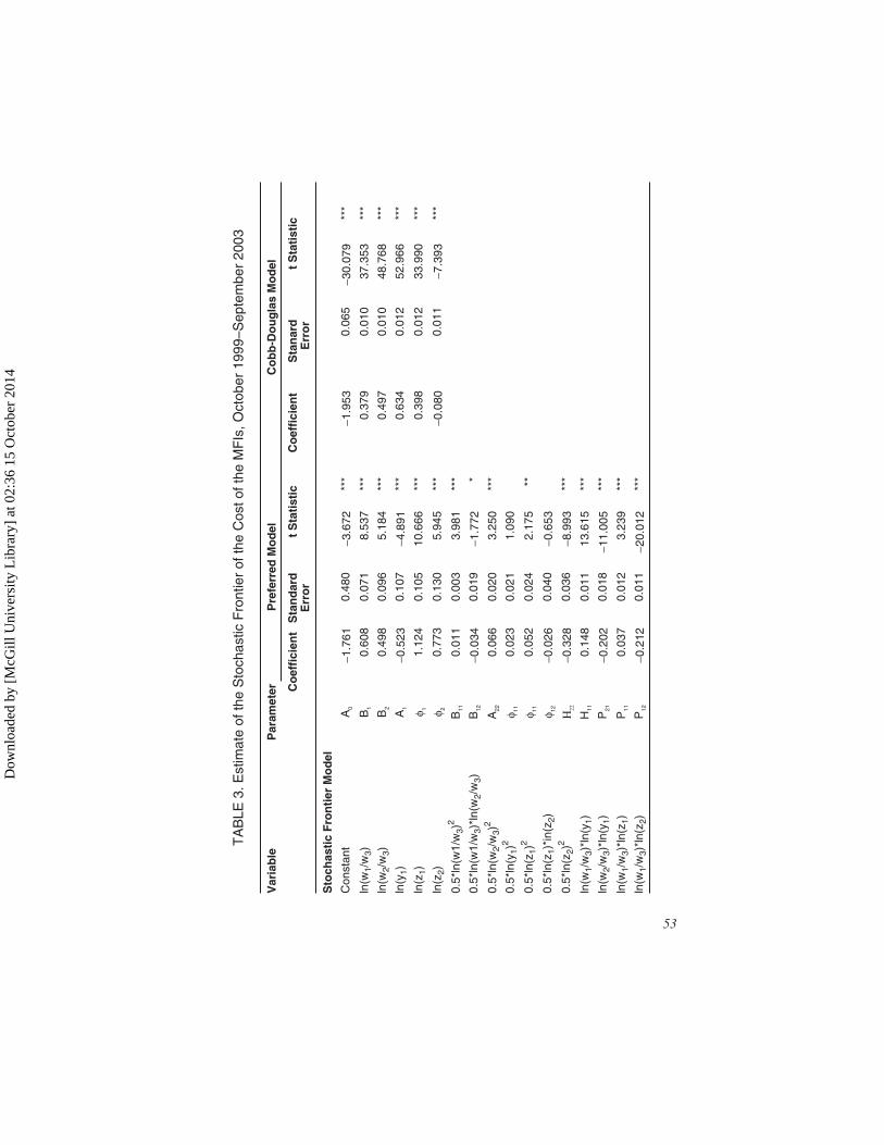
The joint estimate of equations (9) and (10) took place using thegreatest likelihood method proposed by Battese and Coelli (1995) andCoelli (1996). A preferred model was estimated with the translog speci-fication described above in order to compare it with an alternativemodel using the Cobb-Douglas10 specification. The stochastic frontierfindings presented in Table 3 show that most of the estimated parame-ters are significant in both the preferred and the alternative model, al-though they cannot be construed directly as elasticities. The parametersigns are as expected. For an easier presentation and analysis, the ineffi-ciency effect model findings are presented in Section 4.3.


TABLE 2 (continued)

Variable Definition

Financial leverage (APA) Measured by the number of times, calculated by dividing thetotal liabilities by the equity capital and reserves.

Delinquency Rate (MOR) Defined as a percentage of the portfolio in arrears with re-gard to the total direct loans.

Surroundings Variable

Market concentrationIndex (HHI)

Calculated as the weighted sum of the regional concentra-tion rates, 1 using the same weightings as those used for cal-culating the market share. The market concentrationindicator used was the Herfindahl Index, which is defined asthe sum of the square share in direct loans.

Actual GDP (GDP) 2 Measured as the natural algorithm of the actual monthlyGDP.

1Like Maudos (2001), we believe that the regional market is where competition plays an important role.Thus, based on these regional markets, the market costs of each MFI were calculated, along with the re-gional market concentration on which the MFI operates.2It is expected that economic activities should have a positive relationship to inefficiency. As stressed byJanna (2003), periods of expansion are usually followed by lighter pressures to monitor costs, with lowlevels of inefficiency being tolerable, as they do not jeopardize the continuity of the business. In contrast,greater efforts to control costs would be expected during recession periods in order to avoid adverse ef-fects on the sustainability of the MFI, which should upgrade its efficiency levels.

Dow

nloa

ded

by [

McG

ill U

nive

rsity

Lib

rary

] at

02:

36 1

5 O

ctob

er 2

014

TA

BLE

3.E

stim

ate

ofth

eS

toch

astic

Fro

ntie

rof

the

Cos

toft

heM

FIs

,Oct

ober

1999

–Sep

tem

ber

2003

Var

iab

leP

aram

eter

Pre

ferr

edM

od

elC

ob

b-D

ou

gla

sM

od

el

Co

effi

cien

tS

tan

dar

dE

rro

rt

Sta

tist

icC

oef

fici

ent

Sta

nar

dE

rro

rt

Sta

tist

ic

Sto

chas

tic

Fro

nti

erM

od

el

Con

stan

tA

0-1

.761

0.48

0-3

.672

***

-1.9

530.

065

-30.

079

***

ln(w

1/w

3)B

10.

608

0.07

18.

537

***

0.37

90.

010

37.3

53**

*

ln(w

2/w

3)B

20.

498

0.09

65.

184

***

0.49

70.

010

48.7

68**

*

ln(y

1)A

1-0

.523

0.10

7-4

.891

***

0.63

40.

012

52.9

66**

*

ln(z

1)f 1

1.12

40.

105

10.6

66**

*0.

398

0.01

233

.990

***

ln(z

2)f 2

0.77

30.

130

5.94

5**

*-0

.080

0.01

1-7

.393

***

0.5*

ln(w

1/w

3)2

B11

0.01

10.

003

3.98

1**

*

0.5*

ln(w

1/w

3)*l

n(w

2/w

3)B

12-0

.034

0.01

9-1

.772

*

0.5*

ln(w

2/w

3)2

A22

0.06

60.

020

3.25

0**

*

0.5*

ln(y

1)2

f 110.

023

0.02

11.

090

0.5*

ln(z

1)2

f 110.

052

0.02

42.

175

**

0.5*

ln(z

1)*i

n(z 2

)f 12

-0.0

260.

040

-0.6

53

0.5*

ln(z

2)2

H22

-0.3

280.

036

-8.9

93**

*

ln(w

1/w

3)*l

n(y 1

)H

110.

148

0.01

113

.615

***

ln(w

2/w

3)*l

n(y 1

)P

21-0

.202

0.01

8-1

1.00

5**

*

ln(w

1/w

3)*l

n(z 1

)P

110.

037

0.01

23.

239

***

ln(w

1/w

3)*l

n(z 2

)P

12-0

.212

0.01

1-2

0.01

2**

*

53

Dow

nloa

ded

by [

McG

ill U

nive

rsity

Lib

rary

] at

02:

36 1

5 O

ctob

er 2

014

TA

BLE

3(c

ontin

ued)

Var

iab

leP

aram

eter

Pre

ferr

edM

od

elC

ob

b-D

ou

gla

sM

od

el

Co

effi

cien

tS

tan

dar

dE

rro

rt

Sta

tist

icC

oef

fici

ent

Sta

nar

dE

rro

rt

Sta

tist

ic

ln(w

2/w

3)*l

n(z 1

)P

21-0

.018

0.01

7-1

.011

ln(w

2/w

3)*l

n(z 2

)T

220.

234

0.01

416

.286

***

ln(y

1)*l

n(z 1

)T

11-0

.088

0.01

9-4

.601

***

ln(y

1)*l

n(z 2

)T

120.

185

0.02

76.

764

***

Var

ian

ceP

aram

eter

s

Tot

alva

rianc

e( s

sv2

u2+

)Â

20.

047

0.00

317

.416

***

0.19

60.

019

10.2

31**

*

%de

su2

ens

2G

0.77

60.

023

33.4

21**

*0.

932

0.00

910

2.45

1**

*

log

func

tion

likel

ihoo

d10

47.7

4965

9.59

3

No

ofob

serv

atio

ns1,

864

1,86

4

*S

igni

fican

tat9

0%;*

*S

igni

fican

tat9

5%;*

**S

igni

fican

tat9

9%.

54

Dow

nloa

ded

by [

McG

ill U

nive

rsity

Lib

rary

] at

02:

36 1

5 O

ctob

er 2

014

In order to determine the best specification between the translog (noconstraint) and the Cobb-Douglas option (constraint), a Likelihood Ra-tio LR test11 was carried out where the null hypotheses (H0) states thatthe Cobb-Douglas form is a better specification for representing the costfunction of the MFIs. Because the estimated value (l = 776.313) isgreater than the critical statistic at 99% significance and 15 g. l. (30.61),H0 is rejected, meaning the translog specification is a better specifica-tion for the cost function of the MFI.

The stochastic frontier variance parameters are expressed in terms ofs2 = s2

u + s2v and g = s2

u/(s2u + s2

v). This latter parameter shows thatthe contribution of the inefficiency term of the compound residue in thepreferred model reaches 77.6%, indicating that the main source generat-ing the noise around the stochastic frontier is the cost inefficiency of theMFIs.

Hypothesis tests were carried out to determine whether the inclusionof financial capital improved the model adjustment (see Table 4). Thefirst null hypothesis, which specifies financial leverage as the explana-tion for inefficiency, is not significant (i.e., d13 = 0) and is rejected. Thesecond null hypothesis, which specifies the inclusion of financial capi-tal in the cost function, is not significant (i.e., j2 = j12 = j21 = j22 =r12 = r22 = t12 = 0) and is rejected. The third null hypothesis, which con-siders the two previous hypotheses together (i.e.. j2 = j12 = j21 = j22

= r12 = r22 = t12 = d13 = 0), is also rejected. Thus, the importance of fi-nancial capital is clearly shown for estimating the cost efficiency of theFMIs, and this allows us to control, at least theoretically, possible scalebias and the corporate preference for risk.


TABLE 4. Hypothesis Test of the Role Played by Financial Capital When Esti-mating the Cost Efficiency of the MFIs

Hypothesis Log Likelihood LR test Decision

H0: d13 = 0 1,004.449 86.5007 H0 is rejected *

H0: j2 = j12 = j21 = j22 = r12 = r22 = t12 =0

853.507 388.484 H0 is rejected **

H0: j2 = j12 = j21 = j22 = r12 = r22 = t12 =

D13 = 0

814.334 466.830 H0 is rejected **

* Significant at 99% with 1 g. l.** Significant at 99% with 6 g. l.*** Significant at 99% and 7 g. l.

Dow

nloa

ded

by [

McG

ill U

nive

rsity

Lib

rary

] at

02:

36 1

5 O

ctob

er 2

014

4.2 Cost Efficiency Development

Figure 1 shows the average cost efficiency (CE) development by pe-riod or by the period average covered by the study.12 An ongoing in-crease is noted in the average efficiency level, from 0.80% in November1999 to 0.89% in September 2003, with an average of 0.82.13 Thismeans that the MFIs squandered around 18% of the average cost com-pared with the cost located on the frontier. This may be interpreted intwo ways. The 0.82 efficiency means that if the MFIs were on averageproducing at the frontier instead of the current position, only 82% of thefunds used were necessary to produce the same product vector, or alter-natively, the 0.18% inefficiency means that the average of the MFIs re-quires 18% more funds in order to produce the same product vector,compared to an MFI located on the frontier.

Two aspects are particularly noteworthy in the development of the av-erage cost efficiency of the MFIs. First, the standard deviation drops pro-gressively from its peak of 0.190 in February 2000 to 0.090 in August2003, which might well indicate that the companies are increasingly morehomogeneous in terms of resource utilization related to their products,and consequently a firmer consolidation for the micro-financing industry.Second, the steep drops in average cost efficiency are associated with thearrival of new companies into this market. It is interesting to note thatthese companies reach efficiency levels close to the average in aroundone year. For example, Pronegocios EDPYME, which opened for busi-ness in August 2002 at 0.29 efficiency, had reached 0.90 efficiency bySeptember 2003. These new companies are benefiting from the experi-ence of older firms in terms of microcredit technology management(through hiring managers and analysts with credit experience) in paral-lel to market development.


0.90

0.85

0.80

0.75

0.70

Sep

-99

Dec

-99

Mar

-00

Jun-

00

Sep

-00

Dec

-00

Mar

-01

Jun-

01

Sep

-01

Dec

-01

Mar

-02

Jun-

02

Sep

-02

Dec

-02

Mar

-03

Jun-

03

Sep

-03

EC Promedio

FIGURE 1. Average Cost Efficiency Development of the MFIs in PeruDow

nloa

ded

by [

McG

ill U

nive

rsity

Lib

rary

] at

02:

36 1

5 O

ctob

er 2

014

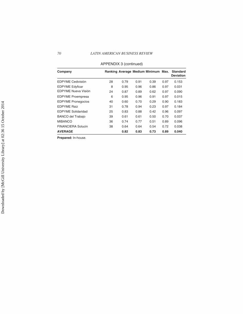
Appendix 3 presents the MFI ranking by the average cost efficiencyfor the period, with some important statistics. The upper quintile of theranking, with an average efficiency of more than 0.95 are the 5 most ef-ficient CMACs, the 2 EDPYMEs and 1 CRAC, while in the bottomquintile of the ranking, with an average efficiency of under 0.75 are the4 least efficient EDPYMEs, 1 CMAC and the three MF banks. It shouldbe pointed out that the largest MFIs in the industry, such as Mibanco,Financiera Solución and Banco del Trabajo are located quite far downthe ranking in 36th, 38th and 39th place, respectively.

4.3 Factors Explaining Differences in Efficiency

The estimated parameters for the inefficiency effect model are of par-ticular interest in this study. As shown in Table 5, most of the estimatedparameters are statistically significant, although the signs are the mostimportant in the analysis.14 The size variable coefficients, meaning thelogarithm for the production assets and the market share, are negativeand statistically significant, indicating that the larger MFIs are the leastinefficient in the industry. They may indicate the existence of econo-mies of scale within the industry.

The coefficient for the dummies that bring together the ownershipand governance characteristics of the firms in the four sectors of this in-dustry (CMAC, CRAC, EDPYMEs and FM Banks) offer positive signsand are statistically significant. Nevertheless, it should be stated that theparameter for the FM Banks is clearly higher than the others, indicatingthat these companies are the most inefficient in the industry.

In addition, it may be observed that there is a negative and statisticallysignificant link between experience and inefficiency, with this findingbeing consistent with what might be expected, since FMIs that havebeen in operation for a longer period of time build up market knowledgeand experience in managing their loan portfolios, allowing them to be-come more efficient.

With regard to the variable that reflects the share held by farm loansin the loans portfolio, a significant negative relation is noted with ineffi-ciency, although weak, when judged by the estimated parameter. Thisunexpected finding might well be influenced by the performance of sev-eral companies, such as the MF Banks, which are the most inefficient,although they do not have farm loans in their portfolios. In turn, the pa-rameter for the variable that reflects the average size of the loan shows asignificant positive relation to inefficiency, evidence that indicates that


Dow

nloa

ded

by [

McG

ill U

nive

rsity

Lib

rary

] at

02:

36 1

5 O

ctob

er 2

014

larger amounts granted to the borrowers−although resulting in lowercosts for each Nuevo Sol lent, increases the inefficiency of the MFIs dueto the credit risk effect that appears when portfolios are concentrated onfewer clients.

It should be stressed that the estimated parameter for the variablescovering the financial management of the MFIs may cause problemswith endogeneity; along these lines, the findings presented should beviewed cautiously. Among them, the most critical is the delinquencyrate (MOR), which is why the model was estimated leaving this variablelagging behind.


TABLE 5. Estimated MFI Inefficiency Effects Model, October 1999-September2003

Variable Parameter Preferred Model Cobb-Douglas Model

Coeffi-cient

StandardError

tstatistic

Coeffi-cient

StandardError

tstatistic

ACT δ1 �0.492 0.020 �24.697 *** �0.928 0.048 �19.259 ***

CUO δ2 �0.272 0.098 �2.794 *** 0.054 0.205 0.265

D1 δ3 1.748 0.812 2.152 ** �10.853 4.344 �2.498 **

D2 δ4 1.880 0.820 2.293 ** �11.330 4.358 �2.600 ***

D3 δ5 1.820 0.824 2.210 ** �10.748 4.356 �2.467 **

D4 δ6 3.915 0.847 4.622 *** �6.991 4.311 �1.622 *

EXP δ7 �0.076 0.022 �3.412 *** �0.135 0.046 �2.965 ***

CAGR δ8 �0.002 0.001 �3.704 *** �0.001 0.001 �1.252

CPRO δ9 0.019 0.002 9.100 *** 0.100 0.005 20.222 ***

DISP δ10 0.010 0.001 11.325 *** 0.022 0.002 12.705 ***

SOSF δ11 0.008 0.016 0.469 �0.073 0.022 �3.266 **

DEP δ12 0.004 0.001 5.714 *** 0.007 0.001 5.773 ***

APA δ13 0.081 0.006 14.737 *** 0.138 0.011 12.080 ***

MOR�1 δ14 0.000 0.001 �0.003 1.347 0.286 4.717 ***

HHI δ15 0.720 0.145 4.965 *** 1.832 0.474 3.864 ***

PBI δ16 0.219 0.090 2.429 ** 0.011 0.003 4.355 ***

* Significant at 90%.** Significant at 95%.*** Significant at 99%.

Dow

nloa

ded

by [

McG

ill U

nive

rsity

Lib

rary

] at

02:

36 1

5 O

ctob

er 2

014

The parameter reflecting the effect of the assets available on effi-ciency shows a significant positive relation, indicating that the MFIswith a higher proportion of cash on hand are more inefficient. A charac-teristic of the good performance achieved by the MFIs is the solvency oftheir liquidity indicators, although there is reason to believe that there isa trade-off between better liquidity indicators and efficiency. In turn,the financial sustainability indicator also shares a significant positiverelation with inefficiency. This unexpected finding might well be due tothe clash between branch managers and shareholders caused by surplusfree cash flows generated by the MFIs, which in turn causes a problemof under-investment and encourages managers to assign funds in lessefficient ways.

Additionally, a significant positive relation is found between the pro-portion of deposits in the corporate liabilities and inefficiency, confirm-ing the fact that over the short term the efforts of the MFIs to replacesources of foreign funding with deposits for financing their activitieshas negative effects on their efficiency due to the higher costs incurredfor mobilizing deposits. Additionally, it is also noted that there is a sig-nificant positive relation between financial leverage and inefficiency.This would show that the solvency risk effect prevails among corporatepreferences for a specific financial structure. This indicates that, in or-der to ensure sustainable growth of MFIs and make good use of econo-mies of scale, regulations should focus on strengthening the equity baseof these companies.

The variable covering the credit risk shows an insignificant nil rela-tion to inefficiency (a similar finding was reached when estimating themodel without discarding this variable).

Looking at the estimated parameters for variables reflecting the ef-fects of the surrounding context, evidence appears for a significant posi-tive relation between market concentration and inefficiency, which isconsistent with the hypothesis that companies operating on more con-centrated markets are subject to less pressure to control their costs, andconsequently are more inefficient. Nevertheless, this finding should beconstrued carefully, as even at the strictly analytical level, there is notnecessarily a positive link between concentration and inefficiency. Inrecent literature, such as Levy-Yeyati and Micco (2003), exactly the op-posite is reported in the experience of several countries.

The parameter reflecting the effect of economic expansion shows asignificant positive relation to inefficiency. This finding shows that dur-ing times of economic expansion, there is less pressure to monitor costs,and certain levels of inefficiency might be tolerable in order to avoid


Dow

nloa

ded

by [

McG

ill U

nive

rsity

Lib

rary

] at

02:

36 1

5 O

ctob

er 2

014

jeopardizing the continuity of the business, while during recession peri-ods, greater effort is expected of managers in terms of cost cutting in or-der to avoid adverse effects on the sustainability of the MFI, enhancingits efficiency levels.

It should be stressed that, according to the estimated parameters, themost important variables affecting efficiency levels are the size of theproduction assets and market concentration, both with the expectedsign. Thus, the main factors determining the cost efficiency of MFIs areassociated with the economies of scale that might well be used by thefirm, as well as the disciplinary framework on the market.

Finally, statistical tests were carried out in order to identify possiblespecification problems in the efficiency effects model. There is a rejec-tion of the hypotheses which state that size and experience, ownershipand governance characteristics, business type and financial manage-ment have not affected inefficiency. The hypothesis that no inefficiencyexists was also rejected.

5. CONCLUSIONS

We have investigated the cost efficiency of MFIs during a periodcharacterized by their dynamic behavior not only in terms of the expan-sion of companies, but also in terms of the entry of new firms into themarket. Through the use of a parametric technique, it was possible toanalyze cost efficiency development and explore the determining fac-tors behind such efficiency levels using variables describing the charac-


Hypothesis Tests on the MFIs Inefficiency Effects Model

Hypothesis Log Likelihood LR Test Decision

H0: �1 = �2 = �7 = 0 919.556 256.387 H0 rejected *

H0: �3 = �4 = �5 = �6 = 0 983.978 127.542 H0 rejected *

H0: �8 = �9 = 0 1,030.150 35.198 H0 rejected *

H0: �10 = �11 = �12 = �13 = �14 = 0 965.153 165.193 H0 rejected *

H0: � = �1 = �2 = �3 = �4 = �5 = �6 = �7 = �8 = �9= �10 = �11 = �12 = �13 = �14 = �15 = �16 = 0

796.236 503.027 H0 rejected *1/

1 The asymptotic distribution of the hypothesis test that involved a constraint of 0 in gamma follows a mixedchi-squared distribution. The critical reference value of this test was taken from A. Kodde and F. Palm(1986). “Wald criteria for jointly testing equality and inequality restrictions,” Econometrica, 54 (5), Table 1,p.1246.

Dow

nloa

ded

by [

McG

ill U

nive

rsity

Lib

rary

] at

02:

36 1

5 O

ctob

er 2

014

teristics of each company, and variables describing the surroundingcontext within which they operate. This showed that the average costsefficiency of the industry is 0.82, and that companies are tending tomanage their funds better, reflected in an increase in the average effi-ciency from 0.80 to 0.89. Judging from the progressive drop in the stan-dard deviation for efficiency throughout each period of time, it may beinferred that the industry is becoming more firmly consolidated. It wasfound that the more efficient companies in the industry with costs effi-ciency levels of over 0.95 are 5 CMACs, 2 EDPYMEs and 1 CRAC; theleast efficient, with costs efficiency levels below 0.75, are the 3 MFBanks and 4 EDPYMEs.

Thus, the potential determining factors for inefficiency were exam-ined, including variables describing the characteristics of each firm andgeneral variables covering the entire industry. According to the esti-mated parameters, the most important variables affecting efficiency areproductive asset size and market concentration. Based on these find-ings, it may be inferred that the main determining factors affecting thecost efficiency of MFIs are associated with economies of scale that canbe used effectively by the company, and the disciplinary framework onthe market.

Evidence was also found that cost efficiency is related negatively tobusiness experience and the proportion of farm loans in the portfolio,related positively to the average loan, the proportion of the variable as-sets, the financial sustainability index, the percentage of deposits fi-nancing the activities of the company, and financial leverage. The riskportfolio is not statistically significant.

With regard to the variable described describing the surroundingcontext, it appears that the increase of the GDP is related positively toinefficiency.

Looking at the governance and ownership structure of the companies,it appears that they are positively related to inefficiency, although amongthem it is the MF Banks that have the most important connection.

NOTES

1. The word microfinance is broader ranging than microcredit. According to themost commonly used definition, microfinance “refers to rendering financial services tolow-income clients, including the self-employed. In general, these financial servicesinclude savings and loans; however, some microfinance organizations also provide in-surance and payment services” (Ledgerwood, 1999, p. 1).


Dow

nloa

ded

by [

McG

ill U

nive

rsity

Lib

rary

] at

02:

36 1

5 O

ctob

er 2

014

In turn, the Peruvian legal framework also institutionalizes this name through Law No26702– General Financial System and Insurance System Act (Ley General del SistemaFinanciero y del Sistema de Seguros) (see www.sbs.gob.pe).

2. According to Decree No 705, a small enterprise is defined as a production unitwith no more than 20 workers and annual sales of less than 20 UIT (US$ 17,806 on De-cember 31, 2003), while micro enterprises are defined as businesses with no more than10 workers and annual sales of less than 12 UIT (US$ 10,684 on October 31, 2003),whose proprietors must work at the company.

3. It is estimated that the SME sector accounts for 42% of the GDP, providing jobsfor 75% of the EAP (Economically Active Population) (Aguilar and Camargo, 2003).

4. The Lima Municipal Peoples Credit Union (La Caja Municipal de Crédito Pop-ular de Lima) does not belong to the CMAC system, since it is regulated by differentlegislation, and has financial technology that is not compatible with that used by thesystem (Chong and Schroth, 1998), which is why it is excluded from this study.

5. For an examination of the development of microfinance institutions in Peru dur-ing the 1990s, see Portocarrero (1999) pp. 13-46.

6. The inclusion of these explicative variables depends on the type of efficiency tobe measured, efficiency in costs, benefits or benefit alternatives.

7. On the importance and consequences of the distributive assumptions, seeGreene (1993), Berger and De Young (1997).

8. Some authors argue that the Flexible Fourier Flexible form provides a better ad-justment, because it adds trigonometric terms to the traditional translog terms; how-ever, Berger and Mester (1997) believe that the difference in the average efficiencybetween the translog and the Fourier form is less than 1%.

9. The estimates were carried out with nominal data without specific treatment ofthe seasonal effects, which we do not regard as relevant for this study because:(1) working with nominal data would not substantially affect the findings, since for theperiod under análisis, inflation remained low in Peru at 3.73% in 1999, 3.73% in 2000,�0.13% in 2001, 1.52% in 2002 and 2.48% in 2003 (the accumulated inflation ratereached 7.58% between October 1999 and September 2003); (2) the database consid-ers flow variables and stock variables whose seasonal behavior is differentiated (infact, the development of some of them shows no seasonal behavior, such as the numberof employees, the number of branches, etc.), which is why any treatment along theselines might generate effects that might not even be controlled further ahead.

10. The Cobb-Douglas specification considers only the first order translog terms.11. The LR test calculates how =�2*[log (likelihood (H0)) �log (likelihood

(H1))], which has a chi-squared distribution level of freedom equal to the number ofconstraints in the null hypothesis.

12. As Frontier 4.1C presents the cost efficiency measurements as exp(ui), in arange of [1, 8], they have been transformed into exp(-ui) in order to ensure that this fallsbetween [0,1] as usually found in the literature.

13. The standard deviation during the period is 0.04%., which means that the in-crease in the CE may be taken as statistically significant with a 90% confidence level.

14. The problems with endogeneity that may appear have been corrected by esti-mating the model without the delinquency rate. It is suggested that the findings forthe variables describing the financial management of the MFIs should be construedwith care.


Dow

nloa

ded

by [

McG

ill U

nive

rsity

Lib

rary

] at

02:

36 1

5 O

ctob

er 2

014

REFERENCES

Aguilar, G., and Camargo, G. (2003). Análisis de la Morosidad de las InstitucionesMicrofinancieras (IMF) en el Perú. Lima: Consorcio de Investigación Económica ySocial, Red de Microcrédito, Genero y Pobreza. 138p.

Battese, G. E., and Coelli, T. J. (1995). “A Model for Technical Inefficiency Effects ina Stochastic Frontier Production Functions for Panel Data,” Empirical Economics,Vol. 20, No. 2, pp. 325-332.

Berger, A. N. (1993). “Distribution-free estimates of efficency in the U. S. banking in-dustry and tests of the standard distributional assumptions,” Journal of ProductivityAnalysis, No. 4, pp. 261-292.

Berger, A. N., and De Young, R. (1997). “Problem Loans and Cost Efficiency in Com-mercial Banks,” Journal of Banking & Finance, Vol. 21, No. 6, pp. 849-870.

Berger, A. N., and Humphrey, D. B. (1997). “Efficiency of Financial Institutions: In-ternational Survey and Directions for Future Research,” European Journal of Oper-ational Research, Vol. 98, No. 2, pp. 175-212.

Berger, A. N., and Mester, L. (1997). “Inside the Black Box: What Explains Differ-ences in the Efficiencies of Financial Institutions?” Journal of Banking & Finance,Vol. 21, No. 4, pp. 895-947.

Chong, A., and Schroth, E. (1998). Cajas Municipales: Microcrédito y Pobreza en elPerú, Lima: Consorcio de Investigación Económica y Social. 110p.

Coelli, T. (1996). “A Guide to Frontier Version 4.1: A Computer Program for Stochas-tic Frontier Production and Cost Function Estimation,” Center for Efficiency andProductivity Analysis Working Paper 96/07, University of New England, Depart-ment of Econometrics, Armidale, Australia.

Fuentes, R., and Vergara, M. (2003). “Explaining Bank Efficiency: Bank Size or Own-ership Structure?” Mimeo. 23p.

Greene, W. H. (1993). “The Econometric Approach to Efficiency Analysis.” in H. O.Fried, C. A. K. Lovell, and S. S. Schmidt (Eds.). The measurement of productive ef-ficiency, techniques and applications, NY: Oxford University Press. pp. 68-119.

Janna, G. M. (2003). “Eficiencia en Costos, Cambios en las Condiciones Generales deMercado y Crisis en la Banca Colombiana: 1992-2002,” Banco de la Republica deColombia, Borradores de Economía, No 260.

León, J. V. (2003). “Exploring the Determinants of Cost Efficiency of MicrofinanceInstitutions,” (draft). México: Universidad Anahuac. 34p.

Levy-Yeyati, E., and Micco, A. (2003). “Concentration and Foreign Penetration inLatin American Banking Sectors: Impact on Competition and Risk,” IDB ResearchDepartment Working Paper, Nº 499.

Maudos, J. (1996). “Eficiencia, Cambio Técnico y Productividad en el Sector BancarioEspañol: una Aproximación de Frontera Estocástica,” Investigaciones económicas,Vol. 20, No. 3, pp. 339-358.

Maudos, J. (2001). “Rentabilidad, Estructura de Mercado y Eficiencia en la Banca.”Revista de Economía Aplicada, Vol. 9, No. 25, pp. 193-207.

Maudos, J., and Pastor, J. M. (2000). “La Eficiencia del Sistema Bancario Español en elContexto de la Unión Europea,” Papeles de Economía Española, No. 84/85,pp. 155-168.


Dow

nloa

ded

by [

McG

ill U

nive

rsity

Lib

rary

] at

02:

36 1

5 O

ctob

er 2

014

Portocarrero, F. (1999). Microfinanzas en el Perú: Experiencias y Perspectivas, Lima:Universidad del Pacifico y PROPYME. 147p.

Portocarrero, F. (2000). “La Oferta Actual de Microcrédito en el Perú,” in F. Porto-carrero, C. Trivelli, and J. Alvarado (2002). Microcrédito en el Perú; QuienesPiden y Quienes Dan Lima: Consorcio de Investigación Económica y Social,pp. 13-84.

SUPERINTENDENCIA DE BANCA Y SEGUROS. Boletín de Instituciones Micro-financieras no Bancarias, Lima. Various issues.

Received: November 9, 2004Accepted: December 15, 2005

doi:10.1300/J140v07n02_03


Dow

nloa

ded

by [

McG

ill U

nive

rsity

Lib

rary

] at

02:

36 1

5 O

ctob

er 2

014

APPENDIX 1

General Information on Microfinance Institutions in Peru(Through September 2003)


No Companies Start-up ofTransac-

tions

No ofBranches

No ofEmployees

Direct Loans

000 S/. %

Total CMAC 136 2 458 1 464 116 42.73

1 CMAC Arequipa 01/23/1986 18 295 294 715 20.13

2 CMAC Chincha 12/22/1997 1 29 11 719 0.80

3 CMAC Cusco 03/28/1988 12 201 132 878 9.08

4 CMAC Del Santa 03/03/1986 7 138 46 805 3.20

5 CMAC Huancayo 08/08/1988 9 187 103 203 7.05

6 CMAC Ica 10/24/1989 10 112 55 705 3.80

7 CMAC Maynas 08/10/1987 8 139 47 186 3.22

8 CMAC Paita 10/25/1989 7 108 38 209 2.61

9 CMAC Pisco 05/02/1992 2 37 11 452 0.78

10 CMAC Piura 01/04/1982 28 487 292 708 19.99

11 CMAC Sullana 12/19/1986 11 253 121 277 8.28

12 CMAC Tacna 06/01/1992 7 163 75 123 5.13

13 CMAC Trujillo 11/12/1984 16 309 233 134 15.92

Total CRAC 56 740 319 759 9.33

14 CRAC Cajamarca 04/03/1995 1 28 12 190 3.8115 CRAC Cajasur 1/ 12/06/1993 7 101 46 700 14.6016 CRAC Chapín 12/12/1994 3 30 8 517 2.66

17 CRAC Cruz deChalpón

03/27/1995 3 42 18 603 5.82

18 CRAC Lib. deAyacucho

05/04/1994 6 53 15 125 4.73

19 CRAC Los Andes 2/ 12/11/1997 1 16 898 1.84

20 CRAC Nor Perú 3/ 03/06/1995 6 3 57 941 18.12

21 CRAC Profinanzas 4/ 03/22/1995 6 56 16 124 5.04

22 CRAC Prymera 02/10/1998 2 38 11 659 3.65

23 CRAC Credinka 11/02/1994 5 69 20 612 6.45

24 CRAC San Martn 5/ 03/20/1994 10 130 60 816 19.02

25 CRAC Señor deLuren

05/23/1994 6 84 45 573 14.25´

Dow

nloa

ded

by [

McG

ill U

nive

rsity

Lib

rary

] at

02:

36 1

5 O

ctob

er 2

014


APPENDIX 1 (continued)

No Companies Start-up ofTransac-

tions

No ofBranches

No ofEmployees

Direct Loans

000 S/. %

TotalEDPYME /EDPYME

53 954 281 653 8.22

26 EDPYME Alternativa 0910/2001 1 14 2 944 1.05

27 EDPYME CamcoPiura

02/01/2001 1 13 1 155 0.41

28 EDPYME Confianza 06/22/1998 6 51 23 843 8.47

29 EDPYME CrearArequipa

04/13/1998 3 95 19 818 7.04

30 EDPYME CrearCusco

03/01/2000 2 15 4 641 1.65

31 EDPYME CrearTacna

04/20/1998 3 43 14 922 5.30

32 EDPYME CrearTrujillo

03/01/2001 1 37 5 361 1.90

33 EDPYME Predivisión 07/17/2000 2 25 5 251 1.86

34 EDPYME Edyficar 01/02/1998 20 351 93 040 33.03

35 EDPYME NuevaVisión

04/20/1998 1 24 9 132 3.24

36 EDPYMEProempresa

01/02/1998 7 99 5 674 2.01

37 EDPYMEPronegocios

08/19/2002 1 29 25 677 9.12

38 EDPYME Raiz 09/20/1999 4 145 66 803 23.72

39 EDPYME Solidaridad 02/03/2000 1 13 3 392 1.20

40 BANCO del Trabajo 08/09/1994 60 2 531 677 132 19.76

41 MIBANCO 05/01/1998 30 823 381 164 11.12

42 FINANCIERA Solucin 1997,aprox 32 1 322 302 819 8.84

TOTAL 367 8 828 3 426 643 100.00

Source: SBS.Prepared: In-house.

Dow

nloa

ded

by [

McG

ill U

nive

rsity

Lib

rary

] at

02:

36 1

5 O

ctob

er 2

014

APPENDIX 2

Ranking of Microfinance Institutions by Indicator Type(Through September 2003)


Companies Overhead/Direct and

indirect loans

Direct loans/Number ofemployees

Direct loans/Numberof offices

Deposits/Direct loans

Indicator Ranking Indicator Ranking Indicator Ranking Indicator Ranking

CMAC Cusco 7.92 1 661.1 3 14,764.2 5 105.49 5

CRAC Cajamarca 9.58 2 435.3 17 12,189.5 9 88.88 16

CMAC Arequipa 9.73 3 999.0 1 17,336.2 1 102.54 6

EDPYME Raiz 10.03 4 460.7 15 16,700.8 2 0.00 41

CMAC Trujillo 10.09 5 754.5 2 15,542.3 4 76.33 22

CRAC Señor deLuren

10.46 6 542.5 7 9,114.7 16 92.46 11

CRAC Caja sur 10.47 7 462.4 13 6,671.4 21 73.93 23

CRAC NorPerú 10.63 8 623.0 4 9,656.9 13 91.41 13

CMAC Piura 11.06 9 601.0 5 16,261.5 3 95.15 8

CMAC Huancayo 11.48 10 551.9 6 11,467.0 11 113.70 3

CMAC Tacna 11.53 11 460.9 14 12,520.5 8 98.60 7

CMAC Ica 12.51 12 497.4 8 6,963.2 18 89.03 15

CMAC Sullana 13.12 13 479.4 9 13,475.2 6 78.08 21

CMAC Del Santa 13.96 14 339.2 24 6,686.5 20 89.82 14

CRAC Credinka 14.10 15 298.7 28 5,153.1 31 122.01 1

EDPYMEConfianza

14.42 16 467.5 11 3,973.8 34 0.00 31

CRAC Libertad. deAyacucho

14.45 17 285.4 30 2,520.9 41 120.98 2

EDPYME NuevaVisión

15.20 18 380.5 19 9,131.8 15 0.00 38

CRAC Cruzde Chalpón

15.27 19 442.9 16 6,201.1 23 93.37 10

CMAC Chincha 16.18 20 404.1 18 11,718.5 10 85.86 18

CMAC Maynas 16.52 21 339.5 23 7,864.3 17 106.73 4

CRAC San Martín 16.73 22 467.8 10 6,757.3 19 93.47 9

CRAC Prymera 16.86 23 306.8 27 5,829.7 25 46.08 28

EDPYME CrearTacna

16.96 24 347.0 22 4,974.0 32 0.00 34

EDPYME CrearArequipa

17.11 25 208.6 39 6,606.1 22 0.00 32

Dow

nloa

ded

by [

McG

ill U

nive

rsity

Lib

rary

] at

02:

36 1

5 O

ctob

er 2

014



Companies Overhead/Direct and

indirect loans

Direct loans/Number ofemployees

Direct loans/Numberof offices

Deposits/Direct loans

Indicator Ranking Indicator Ranking Indicator Ranking Indicator Ranking

CRAC Chapín 17.29 26 283.9 31 2,839.0 38 66.82 24

CRAC Profinanzas 17.84 27 287.9 29 2,687.4 39 51.78 27

EDPYME CrearCusco

17.86 28 309.4 26 4,640.8 33 0.00 33

EDPYME Edyficar 18.70 29 265.1 33 5,815.0 26 0.00 37

CMAC Paita 18.91 30 353.8 21 5,458.5 29 91.62 12

MIBANCO 19.28 31 463.1 12 12,705.5 7 57.03 26

CMAC Pisco 20.94 32 309.5 25 5,726.2 27 82.22 20

EDPYMEProempresa

21.26 33 259.4 35 3,668.1 35 0.00 40

BANCO DELTRABAJO

21.99 34 267.5 32 11,285.5 12 84.37 19

EDPYMESolidaridad

23.29 35 260.9 34 3,391.5 36 0.00 42

CRAC Los Andes 23.63 36 368.6 20 5,897.7 24 61.88 25

EDPYMEPredivisión

24.53 37 210.1 38 2,625.7 40 0.00 36

EDPYME ProNegócios

25.55 38 195.6 40 5,673.7 28 0.00 39

EDPYMEAlternativa

25.75 39 210.3 37 2,944.2 37 0.00 29

FINANCIERASolución

26.51 40 229.1 36 9,463.1 14 87.37 17

EDPYME CrearTrujillo

29.63 41 144.9 41 5,361.2 30 0.00 35

EDPYME CamcoPiura

40.77 42 88.9 42 1,155.2 42 0.00 30

Descriptive Statistics

Average 17.14 388.7 7,890.9 87.39

Médium 16.62 350.4 6,638.8 89.43

Standard deviation 6.55 173.1 4,382.8 18.93

Minimum 7.92 88.9 1,155.2 46.08

Maximum 40.77 999.0 17,336.2 122.01

Prepared: In-house.

Dow

nloa

ded

by [

McG

ill U

nive

rsity

Lib

rary

] at

02:

36 1

5 O

ctob

er 2

014

APPENDIX 3

Costs Efficiency of Microfinance Institutions


Company Ranking Average Medium Minimum Max. StandardDeviation

CMAC Arequipa 2 0.97 0.98 0.94 0.98 0.010

CMAC Chincha 41 0.55 0.83 0.24 0.93 0.254

CMAC Cusco 9 0.95 0.95 0.92 0.98 0.014

CMAC Del Santa 18 0.91 0.93 0.74 0.96 0.055

CMAC Huancayo 12 0.94 0.95 0.88 0.97 0.022

CMAC Ica 3 0.97 0.97 0.96 0.98 0.006

CMAC Maynas 10 0.95 0.95 0.88 0.97 0.022

CMAC Paita 13 0.93 0.94 0.88 0.97 0.016

CMAC Pisco 26 0.81 0.81 0.69 0.90 0.053

CMAC Piura 5 0.96 0.96 0.93 0.98 0.011

CMAC Sullana 4 0.97 0.97 0.96 0.98 0.004

CMAC Tacna 20 0.90 0.93 0.79 0.96 0.044

CMAC Trujillo 1 0.98 0.98 0.97 0.98 0.003

CRAC Cajamarca 30 0.78 0.78 0.69 0.89 0.043

CRAC Cajasur 1/ 14 0.93 0.94 0.77 0.97 0.031

CRAC Chapín 29 0.79 0.86 0.38 0.92 0.120

CRAC Cruz de Chalpón 16 0.92 0.92 0.86 0.99 0.028

CRAC Libertadores de Ayacucho 32 0.77 0.77 0.66 0.87 0.037

CRAC Los Andes 2/ 22 0.88 0.91 0.67 0.95 0.061

CRAC Nor Peru 3/ 11 0.94 0.94 0.91 0.97 0.015

CRAC Profinanzas 4/ 23 0.87 0.89 0.73 0.96 0.051

CRAC Prymera 33 0.76 0.79 0.54 0.94 0.104

CRAC Credinka 21 0.89 0.93 0.75 0.96 0.063

CRAC San Martín 5/ 19 0.90 0.92 0.79 0.96 0.038

CRAC Señor de Luren 7 0.95 0.96 0.88 0.97 0.020

EDPYME Alternativa 34 0.75 0.86 0.33 0.95 0.168

EDPYME Camco Piura 42 0.42 0.46 0.19 0.59 0.098

EDPYME Confianza 27 0.80 0.87 0.51 0.96 0.143

EDPYME Crear Arequipa 17 0.91 0.91 0.83 0.96 0.031

EDPYME Crear Cusco 37 0.65 0.74 0.22 0.91 0.160

EDPYME Crear Tacna 15 0.92 0.95 0.70 0.97 0.054

EDPYME Crear Trujillo 35 0.75 0.83 0.41 0.91 0.124

Dow

nloa

ded

by [

McG

ill U

nive

rsity

Lib

rary

] at

02:

36 1

5 O

ctob

er 2

014



Company Ranking Average Medium Minimum Max. StandardDeviation

EDPYME Cedivisión 28 0.79 0.91 0.39 0.97 0.153

EDPYME Edyficar 8 0.95 0.96 0.86 0.97 0.031EDPYME Nueva Visión 24 0.87 0.89 0.62 0.97 0.090

EDPYME Proempresa 6 0.95 0.96 0.91 0.97 0.015

EDPYME Pronegocios 40 0.60 0.70 0.29 0.90 0.183

EDPYME Raiz 31 0.78 0.94 0.23 0.97 0.184

EDPYME Solidaridad 25 0.83 0.88 0.42 0.96 0.097

BANCO del Trabajo 39 0.61 0.61 0.50 0.70 0.037

MIBANCO 36 0.74 0.77 0.51 0.89 0.096

FINANCIERA Solucin 38 0.64 0.64 0.54 0.72 0.038

AVERAGE 0.82 0.83 0.73 0.89 0.040

Prepared: In-house.

Dow

nloa

ded

by [

McG

ill U

nive

rsity

Lib

rary

] at

02:

36 1

5 O

ctob

er 2

014

cost efficiency of microfinance institutions in peru: a stochastic frontier approach

Documents