cost curves - fep.up.pt · 8.1 long-run cost curves 305 the $50 million isocost line at the new...
TRANSCRIPT
Cost Curves8C H A P T E R
8.1 LONG-RUN COST CURVES
Long-Run Total Cost CurvesHow Does the Long-Run Total Cost Curve Shift When
Input Prices Change?EXAMPLE 8.1 How Would Input Prices Affect the Long-Run
Total Costs for a Trucking Firm?
8.2 LONG-RUN AVERAGE AND MARGINAL COST
What Are Long-Run Average and Marginal Costs?Relationship Between Long-Run Marginal and Average
Cost CurvesEXAMPLE 8.2 The Relationship Between Average and
Marginal Cost in Higher EducationEconomies and Diseconomies of ScaleEXAMPLE 8.3 Economies of Scale in Alumina RefiningEXAMPLE 8.4 Economies of Scale for “Backoffice’’ Activities
in a HospitalReturns to Scale versus Economies of ScaleMeasuring the Extent of Economies of Scale: The
Output Elasticity of Total Cost
8.3 SHORT-RUN COST CURVES
Relationship Between the Long-Run and the Short-RunTotal Cost Curves
Short-Run Marginal and Average CostsThe Long-Run Average Cost Curve as an Envelope
CurveEXAMPLE 8.5 The Short-Run and Long-Run Cost Curves
for an American Railroad Firm
8.4 SPECIAL TOPICS IN COST
Economies of ScopeEXAMPLE 8.6 Nike Enters the Market for Sports EquipmentEconomies of Experience: The Experience CurveEXAMPLE 8.7 The Experience Curve in the Production of
EPROM Chips
8.5 ESTIMATING COST FUNCTIONS*
Constant Elasticity Cost FunctionTranslog Cost FunctionChapter SummaryReview QuestionsProblemsAppendix: Shephard’s Lemma and Duality
What is Shephard’s Lemma?DualityHow Do Total, Average, and Marginal Cost Vary
With Input Prices?Proof of Shephard’s Lemma
7784d_c08_300-345 5/21/01 8:38 AM Page 300
1This example is based on “Latest Merger Boom Is Happening in China and Bears Watching,” Wall Street Journal (July 30, 1997), p. A1 and A9.
301
C H A P T E R P R E V I E W
The Chinese economy in the1990s underwent an unprecedentedboom. As part of that boom, enter-prises such as HiSense Group grewrapidly.1 HiSense, one of China’slargest television producers, increasedits rate of production by 50 percentper year during the mid-1990s. Itsgoal was to transform itself from asleepy domestic producer of televi-sion sets into a consumer electronicsgiant whose brand name was recog-nized throughout Asia.
Of vital concern to HiSense andthe thousands of other Chinese en-terprises that were plotting similar
growth strategies in the late 1990swas how production costs wouldchange as its volume of output in-creased. There is little doubt thatHiSense’s production costs would goup as it produced more television sets.But how fast would they go up?HiSense’s executives hoped that as itproduced more television sets, thecost of each television set would godown, that is, its unit costs will fall asits annual rate of output goes up.
HiSense’s executives also neededto know how input prices would af-fect its production costs. For exam-ple, HiSense competes with other
large Chinese television manufactur-ers to buy up smaller factories. Thiscompetition bids up the price of cap-ital. HiSense had to reckon with theimpact of this price increase on its to-tal production costs.
This chapter is about cost curves—relationships between costs and thevolume of output. It picks up whereChapter 7 left off: with the compara-tive statics of the cost-minimizationproblem. The cost minimization-problem—both in the long run andthe short run—gives rise to total, av-erage, and marginal cost curves. Thischapter studies these curves.
7784d_c08_300-345 5/21/01 8:38 AM Page 301
302 CHAPTER 8 Cost Curves
K (c
apita
l ser
vice
s pe
r ye
ar)
Min
imiz
ed to
tal c
ost
(dol
lars
per
yea
r)
L (labor services per year)(a)
(b)Q (televisions per year)1 million0 2 million
1 million televisions per year
2 million televisions per year
K2
K1
L1 L2
B
B
A
ATC1 = wL1 + rK1
TC2 = wL2 + rK2
TC1 TC2
TC(Q)
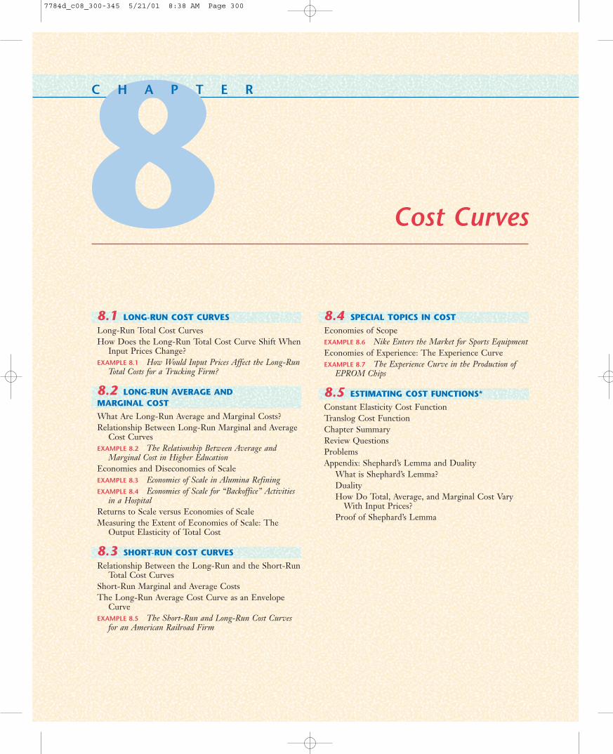
FIGURE 8.1 Cost Minimization and the Long-Run Total Cost Curve for a Producer of Television SetsPanel (a) shows how the solution to the cost-minimization problem for a television pro-ducer changes as output changes from 1 million televisions per year to 2 million televi-sions per year. When output increases, the minimized total cost increases from TC1 toTC2. Panel (b) shows the long-run total cost curve. This curve shows the relationship be-tween the volume of output and the minimum level of total cost the firm can attain whenit produces that output.
LONG-RUN TOTAL COST CURVES
In Chapter 7, we studied the firm’s long-run cost minimization problem and sawhow the cost-minimizing combination of labor and capital depended on the quan-tity of output Q and the prices of labor and capital, w and r. Figure 8.1(a) showshow the optimal input combination for a television firm, such as HiSense, changesas we vary output, holding input prices fixed. For example, when the firm pro-duces 1 million televisions per year, the cost-minimizing input combination oc-curs at point A, with L1 units of labor and K1 units of capital. At this input com-bination, the firm is on an isocost line corresponding to TC1 dollars of total cost,where TC1 � wL1 � rK1. TC1 is thus the minimized total cost when the firm pro-
8.1LONG-RUN
COST CURVES
7784d_c08_300-345 5/21/01 8:38 AM Page 302
8.1 Long-Run Cost Curves 303
duces 1 million units of output. As the firm increases output from 1 million to 2million televisions per year, it ends up on an isocost line further out to point B,with L2 units of labor and K2 units of capital. Thus, its minimized total cost goesup (i.e., TC2 � TC1). It cannot be otherwise, because if the firm could decreasetotal cost by producing more output, it couldn’t have been using a cost-mini-mizing combination of inputs in the first place.
Figure 8.1(b) shows the long-run total cost curve, denoted by TC(Q). Thelong-run total cost curve shows how minimized total cost varies with output, hold-ing input prices fixed. Because the cost-minimizing input combination moves usto higher isocost lines, the long-run total cost curve must be increasing in Q. Wealso know that when Q � 0, long-run total cost is 0. This is because, in the longrun, the firm is free to vary all its inputs, and if it produces a zero quantity, thecost-minimizing input combination is zero labor and zero capital. Thus, com-parative statics analysis of the cost-minimization problem implies that the long-run total cost curve must be increasing and must equal 0, when Q � 0.
E
S
D
LEARNING-BY-DOING EXERCISE 8.1
The Long-Run Total Cost Curve for a Cobb–Douglas Production Function
Let’s return again to the production function Q � 50L�12�K �
12� that we analyzed in
the Learning-By-Doing Exercises in Chapter 7.
Problem
(a) How does minimized total cost depend on the output Q and the inputprices w and r for this production function?
Solution From Learning-By-Doing Exercise 7.4 in Chapter 7, we saw that the following equations described the cost-minimizing quantities of labor andcapital:
L � �5Q0� ��
wr���
12�
(8.1)
K � �5Q0� ��
wr���
12�
(8.2)
To find the minimized total cost, we calculate the total cost the firm incurswhen it uses this cost-minimizing input combination:
TC � w �5Q0� ��
wr���
12�
� r �5Q0� ��
wr���
12�
,
� �5Q0� w �
12�r �
12�
� �5Q0� w�
12�r ��
12�
� Q. (8.3)w�12�r �
12�
�25
7784d_c08_300-345 5/21/01 8:38 AM Page 303
304 CHAPTER 8 Cost Curves
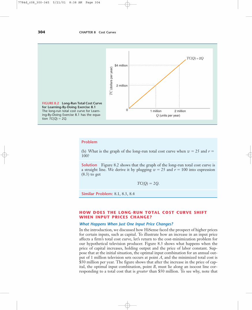
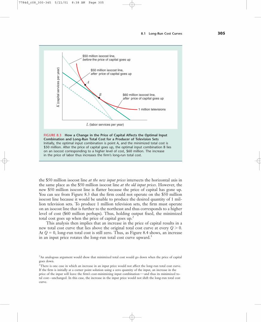
HOW DOES THE LONG-RUN TOTAL COST CURVE SHIFTWHEN INPUT PRICES CHANGE?
What Happens When Just One Input Price Changes?In the introduction, we discussed how HiSense faced the prospect of higher pricesfor certain inputs, such as capital. To illustrate how an increase in an input priceaffects a firm’s total cost curve, let’s return to the cost-minimization problem forour hypothetical television producer. Figure 8.3 shows what happens when theprice of capital increases, holding output and the price of labor constant. Sup-pose that at the initial situation, the optimal input combination for an annual out-put of 1 million television sets occurs at point A, and the minimized total cost is$50 million per year. The figure shows that after the increase in the price of cap-ital, the optimal input combination, point B, must lie along an isocost line cor-responding to a total cost that is greater than $50 million. To see why, note that
Problem
(b) What is the graph of the long-run total cost curve when w � 25 and r �100?
Solution Figure 8.2 shows that the graph of the long-run total cost curve isa straight line. We derive it by plugging w � 25 and r � 100 into expression(8.3) to get
TC(Q) � 2Q.
Similar Problem: 8.1, 8.3, 8.4
TC
(dol
lars
per
yea
r)
Q (units per year)1 million0 2 million
TC(Q) = 2Q
2 million
$4 million
FIGURE 8.2 Long-Run Total Cost Curvefor Learning-By-Doing Exercise 8.1The long-run total cost curve for Learn-ing-By-Doing Exercise 8.1 has the equa-tion TC(Q) � 2Q.
7784d_c08_300-345 5/21/01 8:38 AM Page 304
8.1 Long-Run Cost Curves 305
the $50 million isocost line at the new input prices intersects the horizontal axis inthe same place as the $50 million isocost line at the old input prices. However, thenew $50 million isocost line is flatter because the price of capital has gone up.You can see from Figure 8.3 that the firm could not operate on the $50 millionisocost line because it would be unable to produce the desired quantity of 1 mil-lion television sets. To produce 1 million television sets, the firm must operateon an isocost line that is further to the northeast and thus corresponds to a higherlevel of cost ($60 million perhaps). Thus, holding output fixed, the minimizedtotal cost goes up when the price of capital goes up.2
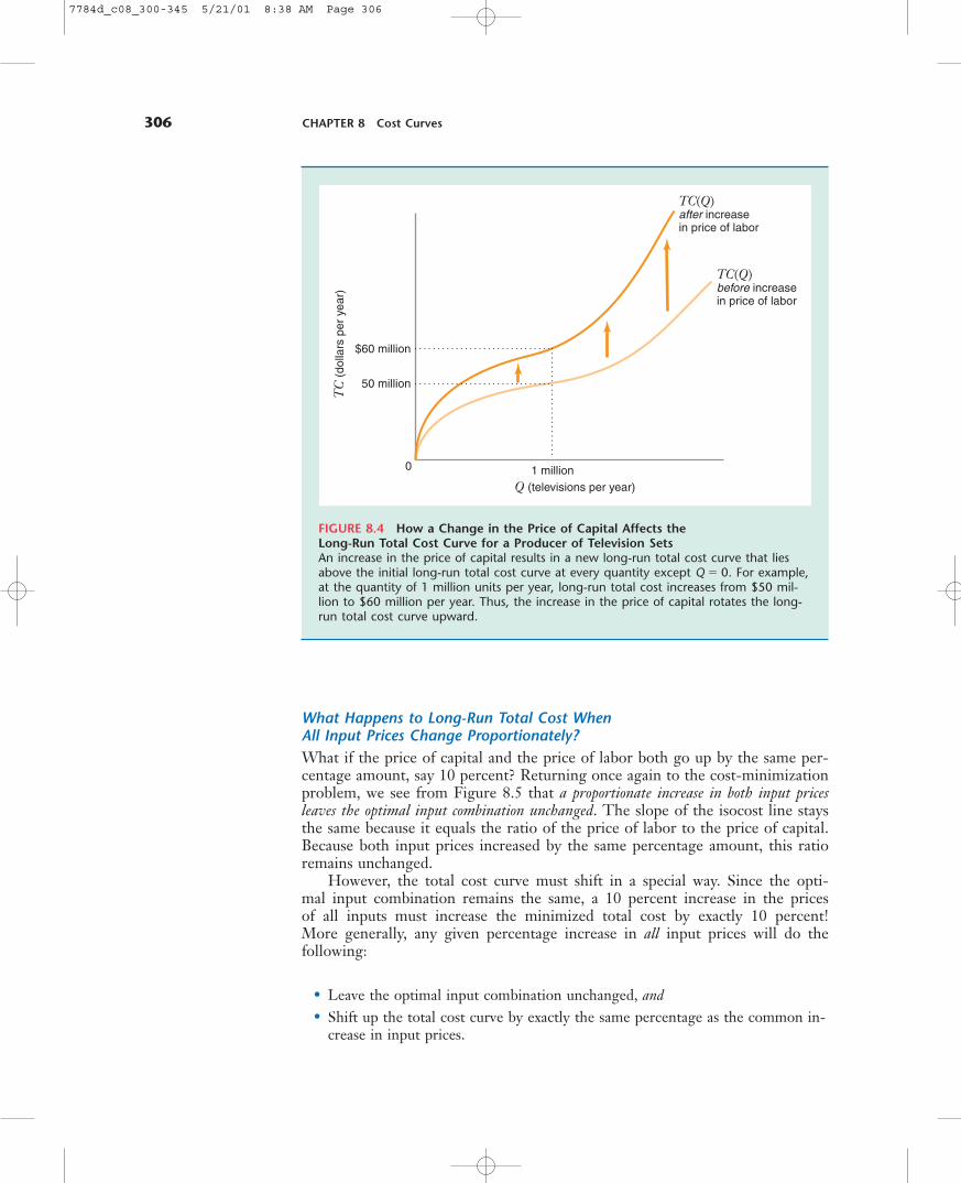
This analysis then implies that an increase in the price of capital results in anew total cost curve that lies above the original total cost curve at every Q � 0.At Q � 0, long-run total cost is still zero. Thus, as Figure 8.4 shows, an increasein an input price rotates the long-run total cost curve upward.3
2An analogous argument would show that minimized total cost would go down when the price of capitalgoes down.3There is one case in which an increase in an input price would not affect the long-run total cost curve.If the firm is initially at a corner point solution using a zero quantity of the input, an increase in theprice of the input will leave the firm’s cost-minimizing input combination—and thus its minimized to-tal cost—unchanged. In this case, the increase in the input price would not shift the long-run total costcurve.
K (c
apita
l ser
vice
s pe
r ye
ar)
L (labor services per year)
1 million televisions
$50 million isocost line,before the price of capital goes up
$50 million isocost line,after price of capital goes up
$60 million isocost line,after price of capital goes up
B
A
FIGURE 8.3 How a Change in the Price of Capital Affects the Optimal Input Combination and Long-Run Total Cost for a Producer of Television SetsInitially, the optimal input combination is point A, and the minimized total cost is $50 million. After the price of capital goes up, the optimal input combination B lies on an isocost corresponding to a higher level of cost, $60 million. The increase in the price of labor thus increases the firm’s long-run total cost.
7784d_c08_300-345 5/21/01 8:38 AM Page 305
306 CHAPTER 8 Cost Curves
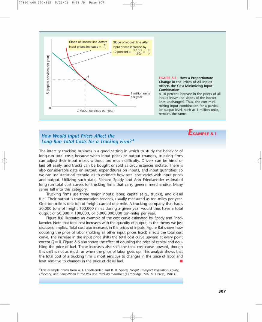
What Happens to Long-Run Total Cost When All Input Prices Change Proportionately?What if the price of capital and the price of labor both go up by the same per-centage amount, say 10 percent? Returning once again to the cost-minimizationproblem, we see from Figure 8.5 that a proportionate increase in both input pricesleaves the optimal input combination unchanged. The slope of the isocost line staysthe same because it equals the ratio of the price of labor to the price of capital.Because both input prices increased by the same percentage amount, this ratioremains unchanged.
However, the total cost curve must shift in a special way. Since the opti-mal input combination remains the same, a 10 percent increase in the prices of all inputs must increase the minimized total cost by exactly 10 percent! More generally, any given percentage increase in all input prices will do the following:
• Leave the optimal input combination unchanged, and• Shift up the total cost curve by exactly the same percentage as the common in-
crease in input prices.
TC
(dol
lars
per
yea
r)
Q (televisions per year)1 million0
TC(Q)after increasein price of labor
TC(Q)before increasein price of labor
50 million
$60 million
FIGURE 8.4 How a Change in the Price of Capital Affects the Long-Run Total Cost Curve for a Producer of Television SetsAn increase in the price of capital results in a new long-run total cost curve that liesabove the initial long-run total cost curve at every quantity except Q � 0. For example,at the quantity of 1 million units per year, long-run total cost increases from $50 mil-lion to $60 million per year. Thus, the increase in the price of capital rotates the long-run total cost curve upward.
7784d_c08_300-345 5/21/01 8:38 AM Page 306
K (c
apita
l ser
vice
s pe
r ye
ar)
L (labor services per year)0
1 million unitsper year
wr
Slope of isocost line before
input prices increase = −
A
wr
1.10w1.10r
Slope of isocost line after
input prices increase by
10 percent = − = −
FIGURE 8.5 How a ProportionateChange in the Prices of All Inputs Affects the Cost-Minimizing InputCombinationA 10 percent increase in the prices of allinputs leaves the slopes of the isocostlines unchanged. Thus, the cost-mini-mizing input combination for a particu-lar output level, such as 1 million units,remains the same.
EXAMPLE 8.1How Would Input Prices Affect the Long-Run Total Costs for a Trucking Firm? 4
The intercity trucking business is a good setting in which to study the behavior oflong-run total costs because when input prices or output changes, trucking firmscan adjust their input mixes without too much difficulty. Drivers can be hired orlaid off easily, and trucks can be bought or sold as circumstances dictate. There isalso considerable data on output, expenditures on inputs, and input quantities, sowe can use statistical techniques to estimate how total cost varies with input pricesand output. Utilizing such data, Richard Spady and Ann Friedlaender estimatedlong-run total cost curves for trucking firms that carry general merchandise. Manysemis fall into this category.
Trucking firms use three major inputs: labor, capital (e.g., trucks), and dieselfuel. Their output is transportation services, usually measured as ton-miles per year.One ton-mile is one ton of freight carried one mile. A trucking company that hauls50,000 tons of freight 100,000 miles during a given year would thus have a totaloutput of 50,000 � 100,000, or 5,000,000,000 ton-miles per year.
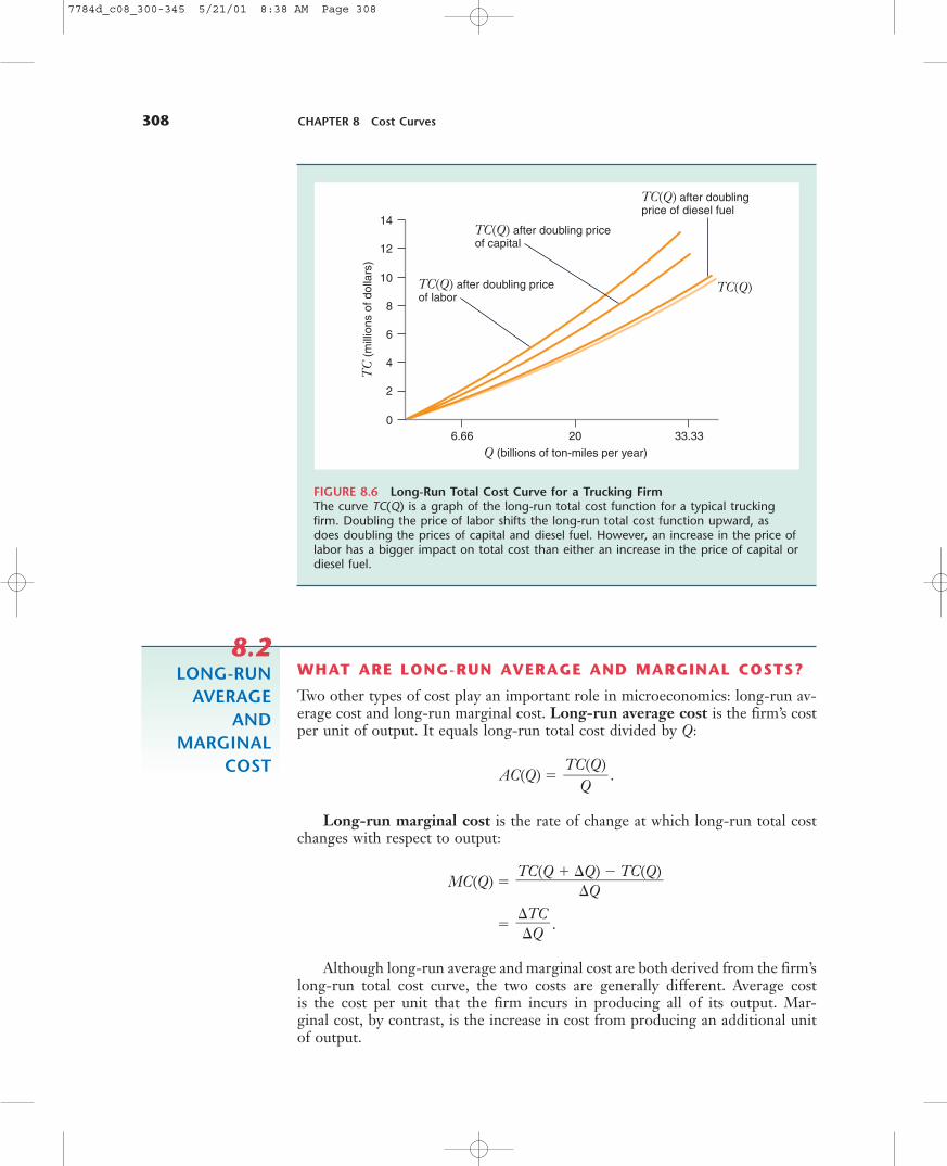
Figure 8.6 illustrates an example of the cost curve estimated by Spady and Fried-laender. Note that total cost increases with the quantity of output, as the theory we justdiscussed implies. Total cost also increases in the prices of inputs. Figure 8.6 shows howdoubling the price of labor (holding all other input prices fixed) affects the total costcurve. The increase in the input price shifts the total cost curve upward at every pointexcept Q � 0. Figure 8.6 also shows the effect of doubling the price of capital and dou-bling the price of fuel. These increases also shift the total cost curve upward, thoughthis shift is not as much as when the price of labor goes up. This analysis shows thatthe total cost of a trucking firm is most sensitive to changes in the price of labor andleast sensitive to changes in the price of diesel fuel. �
4This example draws from A. F. Friedlaender, and R. H. Spady, Freight Transport Regulation: Equity,Efficiency, and Competition in the Rail and Trucking Industries (Cambridge, MA: MIT Press, 1981).
307
7784d_c08_300-345 5/21/01 8:38 AM Page 307
308 CHAPTER 8 Cost Curves
TC
(m
illio
ns o
f dol
lars
)
Q (billions of ton-miles per year)
6.66 20 33.33
TC(Q) after doublingprice of diesel fuel
TC(Q) after doubling priceof labor
TC(Q) after doubling priceof capital
TC(Q)
14
12
10
8
6
4
2
0
FIGURE 8.6 Long-Run Total Cost Curve for a Trucking FirmThe curve TC(Q) is a graph of the long-run total cost function for a typical truckingfirm. Doubling the price of labor shifts the long-run total cost function upward, asdoes doubling the prices of capital and diesel fuel. However, an increase in the price oflabor has a bigger impact on total cost than either an increase in the price of capital ordiesel fuel.
WHAT ARE LONG-RUN AVERAGE AND MARGINAL COSTS?
Two other types of cost play an important role in microeconomics: long-run av-erage cost and long-run marginal cost. Long-run average cost is the firm’s costper unit of output. It equals long-run total cost divided by Q:
AC(Q) � .
Long-run marginal cost is the rate of change at which long-run total costchanges with respect to output:
MC(Q) �
� .
Although long-run average and marginal cost are both derived from the firm’slong-run total cost curve, the two costs are generally different. Average cost is the cost per unit that the firm incurs in producing all of its output. Mar-ginal cost, by contrast, is the increase in cost from producing an additional unitof output.
�TC��Q
TC(Q � �Q) � TC(Q)���
�Q
TC(Q)�
Q
8.2LONG-RUN
AVERAGEAND
MARGINALCOST
7784d_c08_300-345 5/21/01 8:38 AM Page 308
8.2 Long-Run Average and Marginal Cost 309
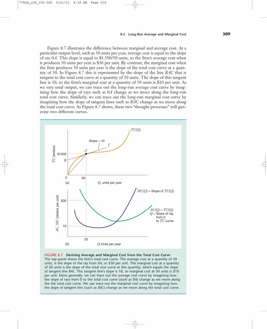
Figure 8.7 illustrates the difference between marginal and average cost. At aparticular output level, such as 50 units per year, average cost is equal to the slopeof ray 0A. This slope is equal to $1,500/50 units, so the firm’s average cost whenit produces 50 units per year is $30 per unit. By contrast, the marginal cost whenthe firm produces 50 units per year is the slope of the total cost curve at a quan-tity of 50. In Figure 8.7 this is represented by the slope of the line BAC that istangent to the total cost curve at a quantity of 50 units. The slope of this tangentline is 10, so the firm’s marginal cost at a quantity of 50 units is $10 per unit. Aswe vary total output, we can trace out the long-run average cost curve by imag-ining how the slope of rays such as 0A change as we move along the long-runtotal cost curve. Similarly, we can trace out the long-run marginal cost curve byimagining how the slope of tangent lines such as BAC change as we move alongthe total cost curve. As Figure 8.7 shows, these two “thought processes” will gen-erate two different curves.
TC
(do
llars
)A
C, M
C (
dolla
rs p
er u
nit)
Q, units per year
Q Units per year
50
50
Slope = 10
0
(a)
(b)
B
AC
AC(Q) = TC(Q)Q = Slope of ray from 0 to TC curve
MC(Q) = Slope of TC(Q)
$1500
$30
10
TC(Q)
FIGURE 8.7 Deriving Average and Marginal Cost from the Total Cost CurveThe top panel shows the firm’s total cost curve. The average cost at a quantity of 50units, is the slope of the ray from 0A, or $30 per unit. The marginal cost at a quantityof 50 units is the slope of the total cost curve at this quantity, which equals the slopeof tangent line BAC. This tangent line’s slope is 10, so marginal cost at 50 units is $10per unit. More generally, we can trace out the average cost curve by imagining howthe slope of rays from 0 to the total cost curve (such as 0A) change as we move alongthe the total cost curve. We can trace out the marginal cost curve by imagining howthe slope of tangent line (such as BAC) change as we move along the total cost curve.
7784d_c08_300-345 5/21/01 8:38 AM Page 309
310 CHAPTER 8 Cost Curves
E
S
D
LEARNING-BY-DOING EXERCISE 8.2
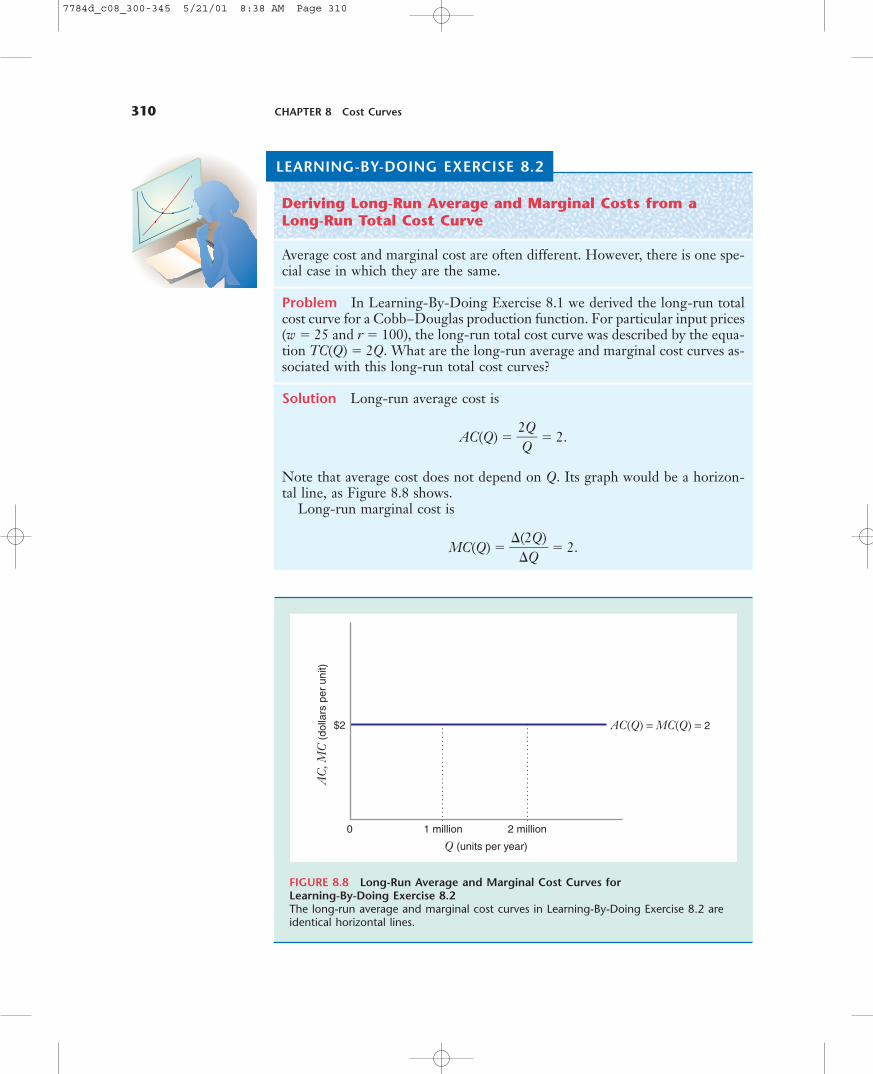
Deriving Long-Run Average and Marginal Costs from a Long-Run Total Cost Curve
Average cost and marginal cost are often different. However, there is one spe-cial case in which they are the same.
Problem In Learning-By-Doing Exercise 8.1 we derived the long-run totalcost curve for a Cobb–Douglas production function. For particular input prices(w � 25 and r � 100), the long-run total cost curve was described by the equa-tion TC(Q) � 2Q. What are the long-run average and marginal cost curves as-sociated with this long-run total cost curves?
Solution Long-run average cost is
AC(Q) � �2QQ� � 2.
Note that average cost does not depend on Q. Its graph would be a horizon-tal line, as Figure 8.8 shows.
Long-run marginal cost is
MC(Q) � ��
�
(2QQ)� � 2.
AC
, MC
(dol
lars
per
uni
t)
Q (units per year)
AC(Q) = MC(Q) = 2$2
1 million0 2 million
FIGURE 8.8 Long-Run Average and Marginal Cost Curves for Learning-By-Doing Exercise 8.2The long-run average and marginal cost curves in Learning-By-Doing Exercise 8.2 areidentical horizontal lines.
7784d_c08_300-345 5/21/01 8:38 AM Page 310
8.2 Long-Run Average and Marginal Cost 311
RELATIONSHIP BETWEEN LONG-RUN MARGINAL ANDAVERAGE COST CURVES
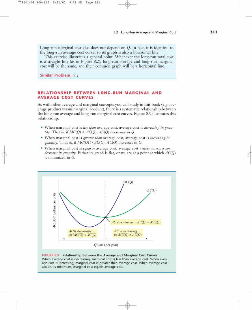
As with other average and marginal concepts you will study in this book (e.g., av-erage product versus marginal product), there is a systematic relationship betweenthe long-run average and long-run marginal cost curves. Figure 8.9 illustrates thisrelationship:
• When marginal cost is less than average cost, average cost is decreasing in quan-tity. That is, if MC(Q) AC(Q), AC(Q) decreases in Q.
• When marginal cost is greater than average cost, average cost is increasing inquantity. Thus is, if MC(Q) � AC(Q), AC(Q) increases in Q.
• When marginal cost is equal to average cost, average cost neither increases nordecreases in quantity. Either its graph is flat, or we are at a point at which AC(Q)is minimized in Q.
AC
, MC
(dol
lars
per
uni
t)
Q (units per year)
AC is increasing,so MC(Q) > AC(Q)
AC is decreasing,so MC(Q) < AC(Q)
AC at a minimum, AC(Q) = MC(Q)
AC(Q)
MC(Q)
FIGURE 8.9 Relationship Between the Average and Marginal Cost CurvesWhen average cost is decreasing, marginal cost is less than average cost. When aver-age cost is increasing, marginal cost is greater than average cost. When average costattains its minimum, marginal cost equals average cost.
Long-run marginal cost also does not depend on Q. In fact, it is identical tothe long-run average cost curve, so its graph is also a horizontal line.
This exercise illustrates a general point. Whenever the long-run total costis a straight line (as in Figure 8.2), long-run average and long-run marginalcost will be the same, and their common graph will be a horizontal line.
Similar Problem: 8.2
7784d_c08_300-345 5/21/01 8:38 AM Page 311
312 CHAPTER 8 Cost Curves
The relationship between marginal cost and average cost is the same as therelationship between the marginal of anything and the average of anything. Toillustrate this point, suppose that the average height of students in your class is160 cm. Now, a new student, Mike Margin, joins the class, and the average heightrises to 161 cm. What do we know about his height? Since the average height isincreasing, the “marginal height” (Mike Margin’s height) must be above the av-erage. If the average height had fallen to 159 cm, it would have been because hisheight was below the average. Finally, if the average height had remained thesame when Mr. Margin joined the class, his height had to exactly equal the av-erage height in the class.
The relationship between average and marginal height in your class is thesame as the relationship between average and marginal product that we observedin Chapter 6. It is also the relationship between average and marginal cost thatwe just described. And it is the relationship between average and marginal rev-enue that we will study in Chapter 11.
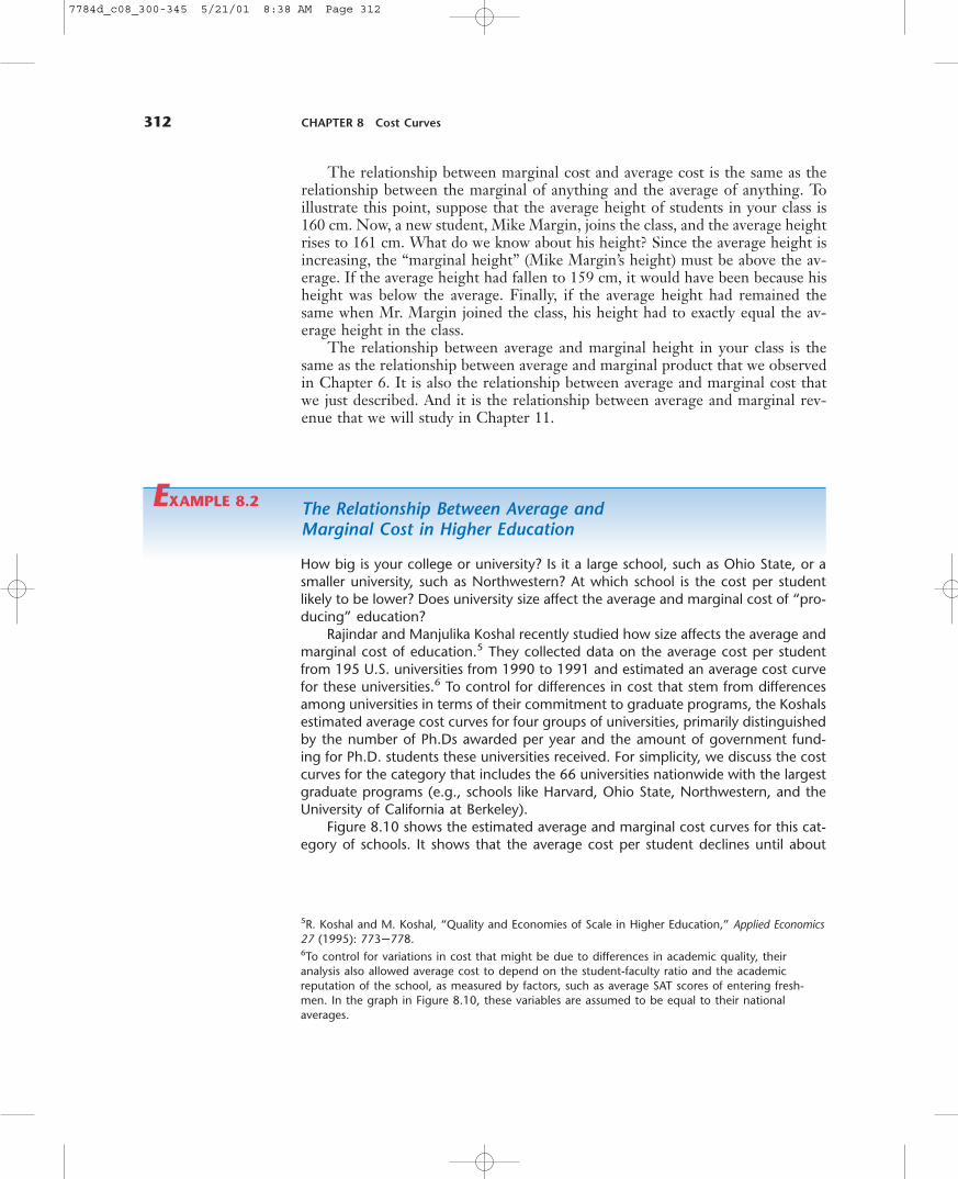
EXAMPLE 8.2 The Relationship Between Average and Marginal Cost in Higher Education
How big is your college or university? Is it a large school, such as Ohio State, or asmaller university, such as Northwestern? At which school is the cost per studentlikely to be lower? Does university size affect the average and marginal cost of “pro-ducing” education?
Rajindar and Manjulika Koshal recently studied how size affects the average andmarginal cost of education.5 They collected data on the average cost per studentfrom 195 U.S. universities from 1990 to 1991 and estimated an average cost curvefor these universities.6 To control for differences in cost that stem from differencesamong universities in terms of their commitment to graduate programs, the Koshalsestimated average cost curves for four groups of universities, primarily distinguishedby the number of Ph.Ds awarded per year and the amount of government fund-ing for Ph.D. students these universities received. For simplicity, we discuss the costcurves for the category that includes the 66 universities nationwide with the largestgraduate programs (e.g., schools like Harvard, Ohio State, Northwestern, and theUniversity of California at Berkeley).
Figure 8.10 shows the estimated average and marginal cost curves for this cat-egory of schools. It shows that the average cost per student declines until about
5R. Koshal and M. Koshal, “Quality and Economies of Scale in Higher Education,” Applied Economics27 (1995): 773–778.6To control for variations in cost that might be due to differences in academic quality, their analysis also allowed average cost to depend on the student-faculty ratio and the academic reputation of the school, as measured by factors, such as average SAT scores of entering fresh-men. In the graph in Figure 8.10, these variables are assumed to be equal to their national averages.
7784d_c08_300-345 5/21/01 8:38 AM Page 312
8.2 Long-Run Average and Marginal Cost 313
30,000 full-time undergraduate students (about the size of Indiana University, forexample). Because few universities are this large, the Koshals’ research suggests thatfor most universities in the United States with large graduate programs, the mar-ginal cost of an additional undergraduate student is less than the average cost perstudent, and thus an increase in the size of the undergraduate student body wouldreduce the cost per student.
This finding seems to make sense. Think about your university. It already has alibrary and buildings for classrooms. It already has a president and a staff to runthe school. These costs will probably not go up much if more students are added.Adding additional students is, of course, not costless. For example, more classesmight have to be added. But it is not that difficult to find people who are able andwilling to teach university classes (e.g., graduate students). Until the point is reachedat which more dormitories or additional classrooms are needed, the extra costs ofmore students are not likely to be that large. Thus, for the typical university, whilethe average cost per student might be fairly high, the marginal cost of matriculat-ing an additional student is often fairly low. If so, average cost will decrease withthe number of students. �
AC
, MC
(do
llars
per
stu
dent
)
Q (thousands of full-time students)
10 30 4020 50
MC
AC
$50,000
40,000
30,000
20,000
10,000
0
FIGURE 8.10 The Average and Marginal Cost Curves for University Education at U.S. UniversitiesThe marginal cost of an additional student is less than the average cost per student un-til enrollment reaches about 30,000 students. Until that point, average cost per studentfalls with the number of students. Beyond that point, the marginal cost of an addi-tional student exceeds the average cost per student, and average cost increases withthe number of students.
7784d_c08_300-345 5/21/01 8:38 AM Page 313
314 CHAPTER 8 Cost Curves
ECONOMIES AND DISECONOMIES OF SCALE
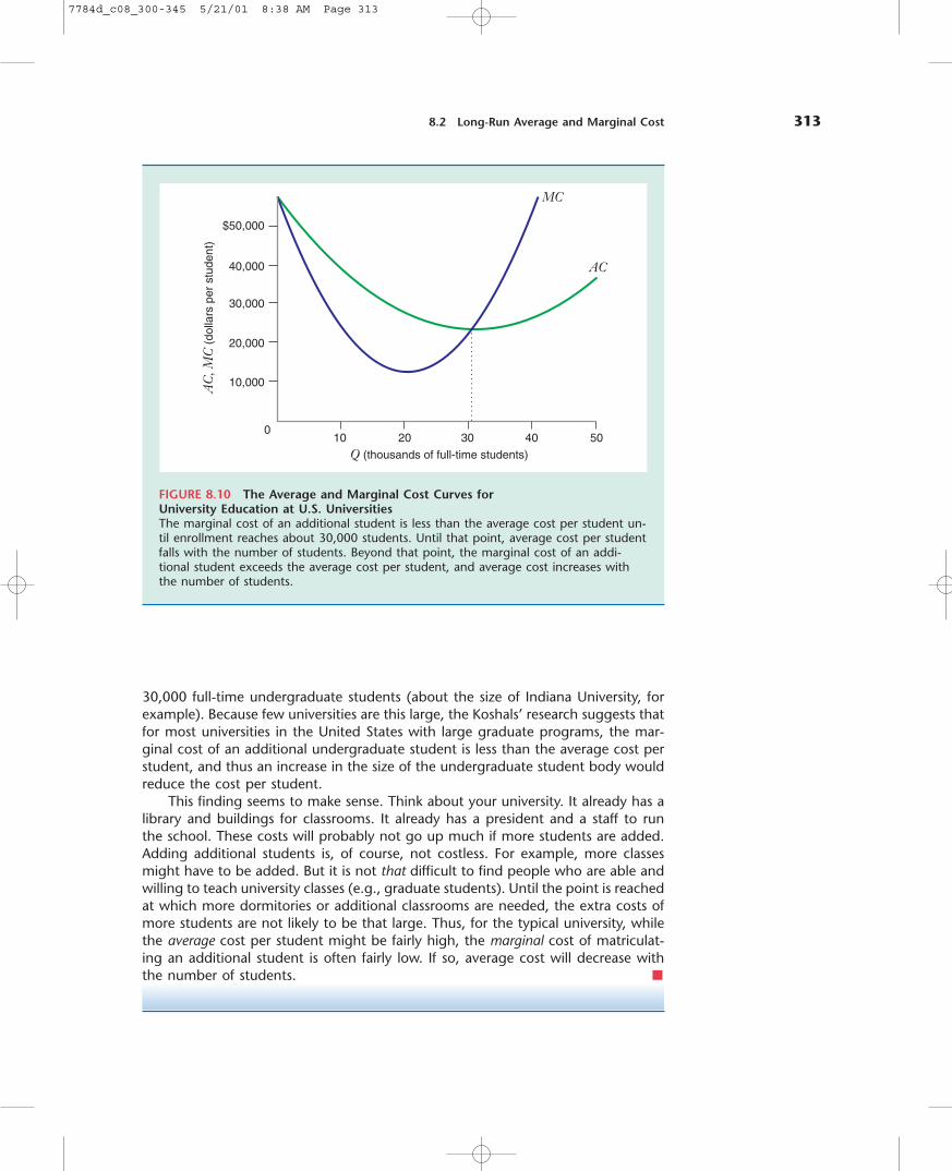
The term economies of scale describes a situation in which average cost de-creases as output goes up, and diseconomies of scale describes the opposite: av-erage cost increases as output goes up. Economies and diseconomies of scale areimportant concepts. The extent of economies of scale can affect the structure ofan industry. Economies of scale can also explain why some firms are more prof-itable than others in the same industry. Claims of economies of scale are oftenused to justify mergers between two firms producing the same product.7
Figure 8.11 illustrates economies and diseconomies of scale by showing anaverage cost curve that many economists believe typifies real-world productionprocesses. For this average cost curve, there is an initial range of economies ofscale (0 to Q), followed by a range over which average cost is flat (Q to Q�), andeventually a range of diseconomies of scale (Q � Q�).
Economies of scale have various causes. They may result from the physical prop-erties of processing units that give rise to increasing returns to scale in inputs (e.g.,the cube-square rule discussed in Chapter 6). Economies of scale can also arise dueto specialization of labor. As the number of workers increases with the output ofthe firm, workers can specialize on tasks, which often increases their productivity.Specialization can also eliminate time-consuming changeovers of workers and equip-ment. This too would increase worker productivity and lower unit costs.
AC
(dol
lars
per
uni
t)
Q (units per year)
AC(Q)
Q′ = minimum efficient scale Q″
FIGURE 8.11 Real-World Average Cost CurveThis average cost curve typifies many real-world production processes. There areeconomies of scale for outputs less than Q. Average costs are flat between Q and Q�,and there are diseconomies of scale thereafter. The output level Q at which theeconomies of scale are exhausted is called the minimum efficient scale.
7See Chapter 4 of F. M. Scherer and D. Ross, Industrial Market Structure and Economic Performance(Boston: Houghton Mifflin) 1990, for a detailed discussion of the implications of economies of scale formarket structure and firm performance.
7784d_c08_300-345 5/21/01 8:38 AM Page 314
8.2 Long-Run Average and Marginal Cost 315
Economies of scale may also result from the need to employ indivisible inputs. An indivisible input is an input that is available only in a certain mini-mum size; its quantity cannot be scaled down as the firm’s output goes to zero.An example of an indivisible input is a high-speed packaging line for breakfastcereal. Even the smallest such lines have huge capacity, 14 million pounds of ce-real per year. A firm that might only want to produce 5 million pounds of ce-real a year would still have to purchase the services of this indivisible piece ofequipment.
Indivisible inputs lead to decreasing average costs (at least over a certain rangeof output) because when a firm purchases the services of an indivisible input, itcan “spread” the cost of the indivisible input over more units of output as out-put goes up. For example, a firm that purchases the services of a minimum-scalepackaging line to produce 5 million pounds of cereal per year will incur the sametotal cost on this input when it increases production to 10 million pounds of ce-real per year.8 This will drive the firm’s average costs down.
The region of diseconomies of scale in Figure 8.11 is usually thought to oc-cur because of managerial diseconomies. Managerial diseconomies arise whena given percentage increase in output forces the firm to increase its spending onthe services of managers by more than this percentage. To see why managerialdiseconomies of scale can arise, imagine an enterprise whose success depends onthe talents or insight of one key individual (e.g., the entrepreneur who startedthe business). As the enterprise grows, that key individual cannot be replicated.To compensate, the firm may have to employ enough additional managers thattotal costs increase at a faster rate than output, which then pushes average costsup. Viewed this way, managerial diseconomies are another example of diminish-ing marginal returns to variable inputs that arise when certain other inputs (spe-cialized managerial talent) are in fixed supply.
The smallest quantity at which the long-run average cost curve attains its minimum point is called the minimum efficient scale, or MES. The MESoccurs at output Q in Figure 8.11. The magnitude of MES relative to the sizeof the market often indicates the magnitude of economies of scale in particularindustries. The larger is MES in comparison to overall market sales, the greaterthe magnitude of economies of scale. Table 8.1 shows MES as a percentage oftotal industry output, for a selected group of U.S. food and beverage indus-tries.9 The industries with the largest MES-market size ratios are breakfast cereal and cane sugar refining. These industries have significant economies ofscale. The industries with the lowest MES-market size ratios are mineral waterand bread. Economies of scale in manufacturing in these industries appear to be weak.
8Of course, it may spend more on other inputs, such as raw materials, that are not indivisible.9In this table, MES is measured as the capacity of the median plant in an industry. The median plant isthe plant whose capacity lies exactly in the middle of the range of capacities of plants in an industry.That is, 50 percent of all plants in particular industry have capacities that are smaller than the medianplant in that industry, and 50 percent have capacities that are larger. Estimates of MES based on the ca-pacity of the median plant correlate highly with “engineering estimates” of MES that are obtained byasking well-informed manufacturing and engineering personnel to provide educated estimates of mini-mum efficient scale plant sizes. Data on median plant size in U.S. industries are available from the U.S.Census of Manufacturing.
7784d_c08_300-345 5/21/01 8:38 AM Page 315

316 CHAPTER 8 Cost Curves
TABLE 8.1MES as a Percentage of Industry Output for Selected U.S. Food and Beverage Industries
EXAMPLE 8.3Economies of Scale in Alumina Refining10
Manufacturing aluminum involves several steps, one of which is alumina refining.Alumina is a chemical compound consisting of aluminum and oxygen atoms (Al2O3).Alumina is created when bauxite ore—the basic raw material used to produce alu-minum—is transformed using a technology known as the Bayer process.
There are substantial economies of scale in the refining of alumina. Table 8.2—drawn from John Stuckey’s study of the aluminum industry—shows estimated long-run average costs as a function of the capacity of an alumina refinery. As plant ca-pacity doubles from 150,000 tons per year to 300,000 tons per year, long-run av-erage cost declines by about 12 percent. Stuckey reports that average costs inalumina refining may continue to fall up to capacities of 500,000. If so, then theminimum efficient scale of an alumina refinery would occur at an output of 500,000tons per year.
If firms understand this, we would expect most alumina plants to have capac-ities of at least 500,000 tons per year. In fact, this is true. In 1979, the average ca-pacity of the 10 alumina refineries in North America was 800,000 tons per year,and only two were under 500,000 tons per year. No alumina refinery’s capacity ex-ceeded 1.3 million tons per year. This suggests that diseconomies of scale set in atabout this level of output. �
10The information in this example draws from J. Stuckey, Vertical Integration and Joint Ventures in the Aluminum Industry (Cambridge, MA: Harvard University Press, 1983), especially pp. 12–14.
MES as MES asIndustry % of Output Industry % of Output
Beet sugar 1.87 Breakfast cereal 9.47
Cane sugar 12.01 Mineral water 0.08
Flour 0.68 Roasted coffee 5.82
Bread 0.12 Pet food 3.02
Canned vegetables 0.17 Baby food 2.59
Frozen food 0.92 Beer 1.37
Margarine 1.75
Source: Table 4.2 in J. Sutton, Sunk Costs and Market Structure: Price Competition,Advertising, and the Evolution of Concentration (Cambridge, MA: MIT Press,1991).
7784d_c08_300-345 5/21/01 8:38 AM Page 316
8.2 Long-Run Average and Marginal Cost 317
TABLE 8.2Plant Capacity and Average Cost in Alumina Refining
Plant Capacity Index of Average Cost(tons) (equals 100 at 300,000 tons)
55,000 139
90,000 124
150,000 114
300,000 100
Source: Table 1-1 in Stuckey, Vertical Integration and Joint Ventures in theAluminum Industry. (Cambridge, MA: Harvard University Press, 1983.)
EXAMPLE 8.4Economies of Scale for “Backoffice” Activities in a Hospital
The business of health care was in the news a lot during the 1990s. One of themost interesting trends was the consolidation of hospitals through mergers. In theChicago area, for example, Northwestern Memorial Hospital merged with severalsuburban hospitals, such as Evanston Hospital, to form a large multi-hospital sys-tem covering the North Side of Chicago and the North Shore.
Proponents of hospital mergers argue that mergers enable hospitals to achievecost savings through economies of scale in “backoffice” operations—activities, suchas laundry, housekeeping, cafeterias, printing and duplicating services, and dataprocessing, that do not generate revenue for a hospital directly, but that the hos-pital cannot function without. Opponents argue that such cost savings are illusoryand that hospital mergers mainly reduce competition in local hospital markets. TheU.S. antitrust authorities have blocked several hospital mergers on this basis.
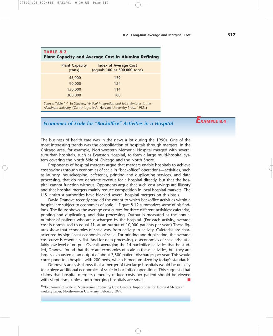
David Dranove recently studied the extent to which backoffice activities within ahospital are subject to economies of scale.11 Figure 8.12 summarizes some of his find-ings. The figure shows the average cost curves for three different activities: cafeterias,printing and duplicating, and data processing. Output is measured as the annualnumber of patients who are discharged by the hospital. (For each activity, averagecost is normalized to equal $1, at an output of 10,000 patients per year.) These fig-ures show that economies of scale vary from activity to activity. Cafeterias are char-acterized by significant economies of scale. For printing and duplicating, the averagecost curve is essentially flat. And for data processing, diseconomies of scale arise at afairly low level of output. Overall, averaging the 14 backoffice activities that he stud-ied, Dranove found that there are economies of scale in these activities, but they arelargely exhausted at an output of about 7,500 patient discharges per year. This wouldcorrespond to a hospital with 200 beds, which is medium-sized by today’s standards.
Dranove’s analysis shows that a merger of two large hospitals would be unlikelyto achieve additional economies of scale in backoffice operations. This suggests thatclaims that hospital mergers generally reduce costs per patient should be viewedwith skepticism, unless both merging hospitals are small. �
11“Economies of Scale in Nonrevenue Producing Cost Centers: Implications for Hospital Mergers,”working paper, Northwestern University, February 1997.
7784d_c08_300-345 5/21/01 8:38 AM Page 317
318 CHAPTER 8 Cost Curves
RETURNS TO SCALE VERSUS ECONOMIES OF SCALE
The concept of economies of scale is closely related to the concept of returns toscale introduced in Chapter 6. The returns to scale of the production functionwill determine how average cost varies with output and thus the existence ofeconomies or diseconomies of scale.
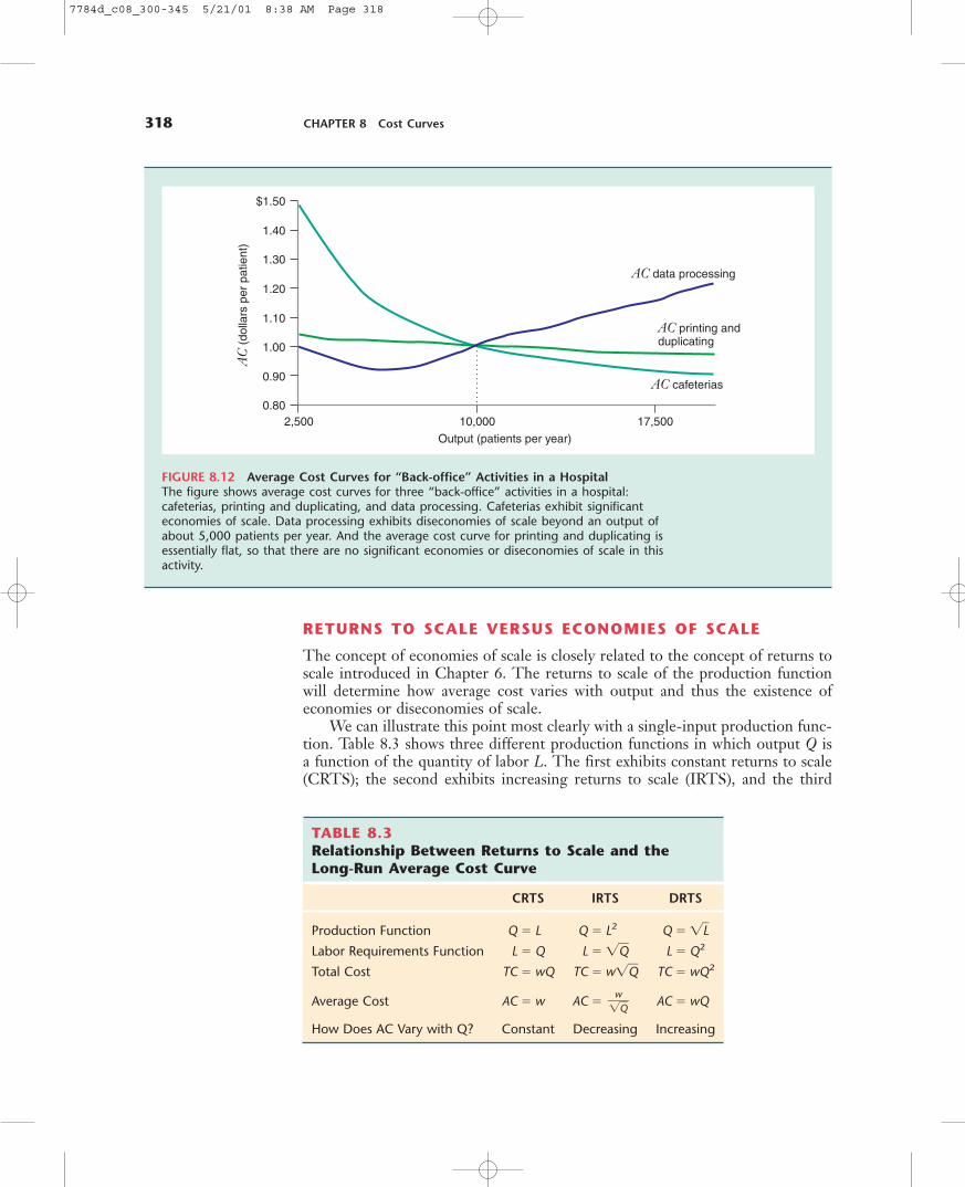
We can illustrate this point most clearly with a single-input production func-tion. Table 8.3 shows three different production functions in which output Q isa function of the quantity of labor L. The first exhibits constant returns to scale(CRTS); the second exhibits increasing returns to scale (IRTS), and the third
AC
(do
llars
per
pat
ient
)
Output (patients per year)
2,500 10,000 17,500
AC printing andduplicating
AC cafeterias
AC data processing
$1.50
1.40
1.30
1.20
1.10
1.00
0.90
0.80
FIGURE 8.12 Average Cost Curves for “Back-office” Activities in a HospitalThe figure shows average cost curves for three “back-office” activities in a hospital: cafeterias, printing and duplicating, and data processing. Cafeterias exhibit significanteconomies of scale. Data processing exhibits diseconomies of scale beyond an output ofabout 5,000 patients per year. And the average cost curve for printing and duplicating isessentially flat, so that there are no significant economies or diseconomies of scale in thisactivity.
TABLE 8.3Relationship Between Returns to Scale and the Long-Run Average Cost Curve
CRTS IRTS DRTS
Production Function Q � L Q � L2 Q � �L�Labor Requirements Function L � Q L � �Q� L � Q2
Total Cost TC � wQ TC � w�Q� TC � wQ2
Average Cost AC � w AC � AC � wQ
How Does AC Vary with Q? Constant Decreasing Increasing
w��Q�
7784d_c08_300-345 5/21/01 8:38 AM Page 318
8.2 Long-Run Average and Marginal Cost 319
exhibits decreasing returns to scale (DRTS). Table 8.3 also shows the labor-requirements functions for these three production functions.12 It also shows ex-pressions for total cost and average cost, given a price of labor w. For the pro-duction function exhibiting constant returns to scale, the average cost function isindependent of the quantity of output (i.e., it equals w no matter what Q is). Forthe production function exhibiting increasing returns to scale, average cost is adecreasing function of the quantity of output Q (i.e., as Q goes up, AC goes down).And for the production function exhibiting decreasing returns to scale, the aver-age cost is an increasing function of output (i.e., as Q goes up, AC also goes up).
This can be summarized in three general relationships:
• When the production function exhibits increasing returns to scale, the long-runaverage cost curve exhibits economies of scale (i.e., AC(Q) must decrease in Q).
• When the production function exhibits decreasing returns to scale, the long-runaverage cost curve exhibits diseconomies of scale (i.e., AC(Q) must increase in Q).
• When the production function exhibits constant returns to scale, the long-run av-erage cost curve is flat: It neither increases nor decreases in output.
MEASURING THE EXTENT OF ECONOMIES OF SCALE: THEOUTPUT ELASTICITY OF TOTAL COST
In Chapter 2, you learned that elasticities of demand, such as the price elasticityof demand or income elasticity of demand, tell us how sensitive demand is to thevarious factors that drive demand, such as price or income. We can also use elas-ticities to tell us how sensitive total cost is to the factors that influence it. An im-portant cost elasticity is the output elasticity of total cost, denoted by �TC,Q. Itis defined as the percentage change in total cost per 1 percent change in output:
�TC,Q � .
We can rewrite this as follows:
�TC,Q � ��
�
TQC
� �TQC� � �
MAC
C�.
Because the output elasticity of total cost is equal to the ratio of marginal to av-erage cost, it tells us whether there are economies of scale or diseconomies ofscale. This is because the following conditions hold:
• If �TC,Q 1, MC AC, so AC decreases in Q, and we have economies of scale.• If �TC,Q � 1, MC AC, so AC increases in Q, and we have diseconomies of scale.• If �TC,Q � 1, MC � AC, so AC neither increases nor decreases in Q.
The output elasticity is often used to characterize the nature of economies of scalein different industries. Table 8.4, for example, shows results of a recent study thatestimated the output elasticity of total cost for several manufacturing industries
��
TTCC
�
�
��
QQ�
12Recall from Chapter 6 that the labor requirements function tells us the quantity of labor needed toproduce a given amount of output.
7784d_c08_300-345 5/21/01 8:38 AM Page 319
320 CHAPTER 8 Cost Curves
TABLE 8.4Estimates of the Output Elasticities for Selected Manufacturing Industries in India
Output ElasticityIndustry of Total Cost
Iron and Steel 0.553
Cotton Textiles 1.211
Cement 1.162
Electricity and Gas 0.3823
The long-run total cost curve shows how the firm’s minimized total cost varieswith output when the firm is free to adjust all its inputs. The short-run total costcurve, STC(Q), tells us the minimized total cost of producing Q units of output when capital is fixed at a particular level, K�.. The short-run total cost curve is the sum of two components: the total variable cost curve,TVC(Q), and the total fixed cost curve TFC (i.e., STC(Q) � TVC(Q) � TFC). Thetotal variable cost curve TVC(Q) is the sum of expenditures on variable inputs, suchas labor and materials, at the short-run cost-minimizing input combination. Totalfixed cost is equal to the cost of the fixed capital services (i.e., TFC � rK�) and thusdoes not vary with output. Figure 8.13 shows a graph of the short-run total costcurve, the total variable cost curve, and the total fixed cost curve.
8.3SHORT-RUN
COST CURVES
E
S
D
LEARNING-BY-DOING EXERCISE 8.3
Deriving the Short-Run Total Cost Curve
Let us return to the production function in Learning-By-Doing Exercise 7.6in Chapter 7. For that production function, the firm uses three inputs: capi-tal, labor, and materials:
Q � K �12�L�
14�M �
14�
13R. Jha, M.N. Murty, S. Paul, and B. Bhaskara Rao, “An Analysis of Technological Change, FactorSubstitution, and Economies of Scale in Manufacturing Industries in India, Applied Economics 25 (Octo-ber 1993): 1337–1343. The estimated output elasticities are reported in Table 5.14The estimated output elasticities for textiles and cement are not statistically different from 1. Thus,these industries might be characterized by constant returns to scale.
in India.13 Iron and steel industries and electricity and gas industries have outputelasticities significantly less than 1, indicating the presence of economies of scale.By contrast, textile and cement firms’ output elasticities are a little higher than1, indicating slight diseconomies of scale.14
7784d_c08_300-345 5/21/01 8:38 AM Page 320
TC
(dol
lars
per
yea
r)
Q (units per year)0
TFC
TFC = rK
TVC(Q)
STC(Q)
rK
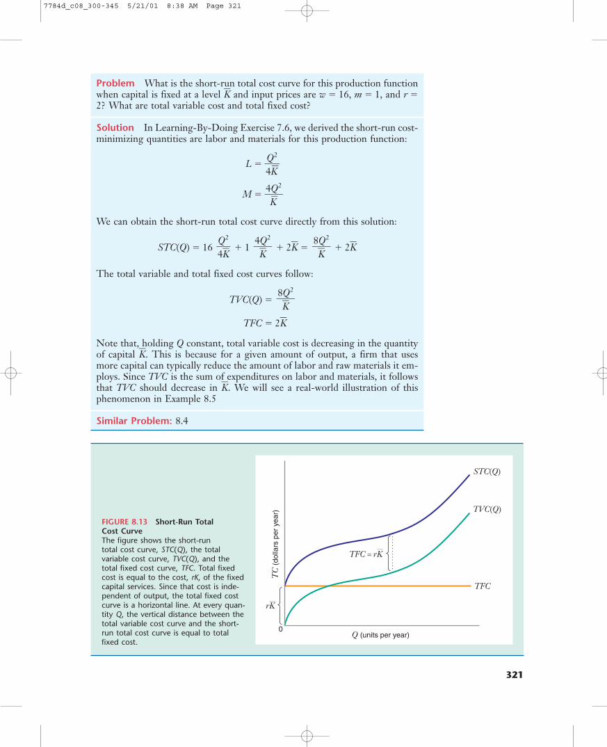
FIGURE 8.13 Short-Run Total Cost CurveThe figure shows the short-run total cost curve, STC(Q), the total variable cost curve, TVC(Q), and the total fixed cost curve, TFC. Total fixedcost is equal to the cost, rK, of the fixedcapital services. Since that cost is inde-pendent of output, the total fixed costcurve is a horizontal line. At every quan-tity Q, the vertical distance between thetotal variable cost curve and the short-run total cost curve is equal to totalfixed cost.
Problem What is the short-run total cost curve for this production functionwhen capital is fixed at a level K� and input prices are w � 16, m � 1, and r �2? What are total variable cost and total fixed cost?
Solution In Learning-By-Doing Exercise 7.6, we derived the short-run cost-minimizing quantities are labor and materials for this production function:
L � �4QK�
2
�
M � �4KQ�
2
�
We can obtain the short-run total cost curve directly from this solution:
STC(Q) � 16 � 1 � 2K� � � 2K�
The total variable and total fixed cost curves follow:
TVC(Q) �
TFC � 2K�
Note that, holding Q constant, total variable cost is decreasing in the quantityof capital K�. This is because for a given amount of output, a firm that usesmore capital can typically reduce the amount of labor and raw materials it em-ploys. Since TVC is the sum of expenditures on labor and materials, it followsthat TVC should decrease in K�. We will see a real-world illustration of thisphenomenon in Example 8.5
Similar Problem: 8.4
8Q2
�K�
8Q2
�K�
4Q2
�K�
Q2
�4K�
321
7784d_c08_300-345 5/21/01 8:38 AM Page 321
322 CHAPTER 8 Cost Curves
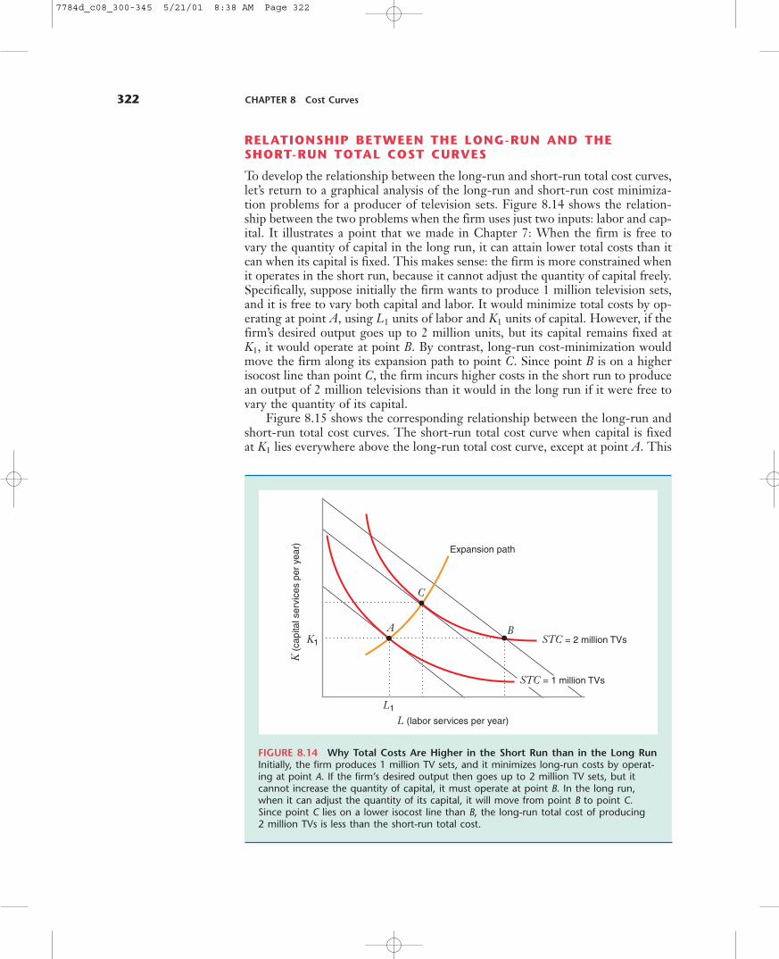
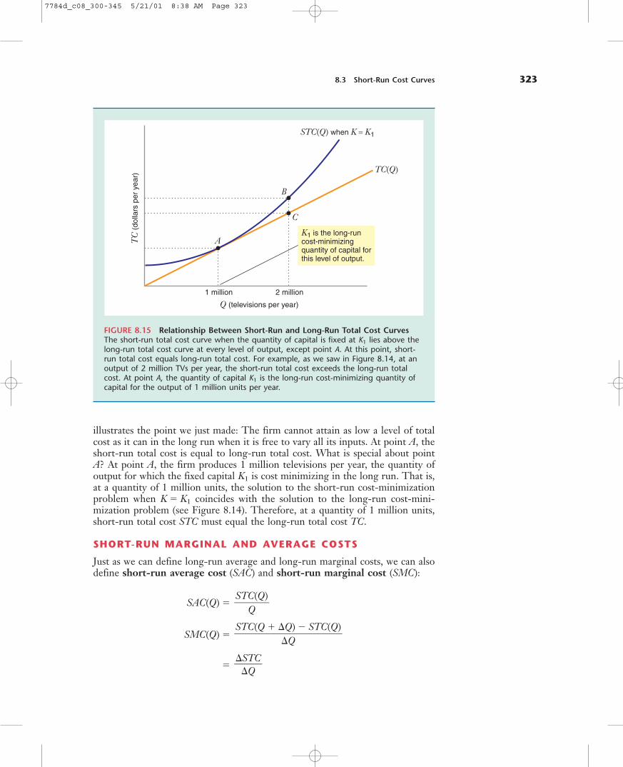
RELATIONSHIP BETWEEN THE LONG-RUN AND THE SHORT-RUN TOTAL COST CURVES
To develop the relationship between the long-run and short-run total cost curves,let’s return to a graphical analysis of the long-run and short-run cost minimiza-tion problems for a producer of television sets. Figure 8.14 shows the relation-ship between the two problems when the firm uses just two inputs: labor and cap-ital. It illustrates a point that we made in Chapter 7: When the firm is free tovary the quantity of capital in the long run, it can attain lower total costs than itcan when its capital is fixed. This makes sense: the firm is more constrained whenit operates in the short run, because it cannot adjust the quantity of capital freely.Specifically, suppose initially the firm wants to produce 1 million television sets,and it is free to vary both capital and labor. It would minimize total costs by op-erating at point A, using L1 units of labor and K1 units of capital. However, if thefirm’s desired output goes up to 2 million units, but its capital remains fixed atK1, it would operate at point B. By contrast, long-run cost-minimization wouldmove the firm along its expansion path to point C. Since point B is on a higherisocost line than point C, the firm incurs higher costs in the short run to producean output of 2 million televisions than it would in the long run if it were free tovary the quantity of its capital.
Figure 8.15 shows the corresponding relationship between the long-run andshort-run total cost curves. The short-run total cost curve when capital is fixedat K1 lies everywhere above the long-run total cost curve, except at point A. This
K (c
apita
l ser
vice
s pe
r ye
ar)
L (labor services per year)
STC = 2 million TVs
Expansion path
K1
L1
B
C
A
STC = 1 million TVs
FIGURE 8.14 Why Total Costs Are Higher in the Short Run than in the Long RunInitially, the firm produces 1 million TV sets, and it minimizes long-run costs by operat-ing at point A. If the firm’s desired output then goes up to 2 million TV sets, but itcannot increase the quantity of capital, it must operate at point B. In the long run,when it can adjust the quantity of its capital, it will move from point B to point C.Since point C lies on a lower isocost line than B, the long-run total cost of producing 2 million TVs is less than the short-run total cost.
7784d_c08_300-345 5/21/01 8:38 AM Page 322
8.3 Short-Run Cost Curves 323
illustrates the point we just made: The firm cannot attain as low a level of totalcost as it can in the long run when it is free to vary all its inputs. At point A, theshort-run total cost is equal to long-run total cost. What is special about pointA? At point A, the firm produces 1 million televisions per year, the quantity ofoutput for which the fixed capital K1 is cost minimizing in the long run. That is,at a quantity of 1 million units, the solution to the short-run cost-minimizationproblem when K � K1 coincides with the solution to the long-run cost-mini-mization problem (see Figure 8.14). Therefore, at a quantity of 1 million units,short-run total cost STC must equal the long-run total cost TC.
SHORT-RUN MARGINAL AND AVERAGE COSTS
Just as we can define long-run average and long-run marginal costs, we can alsodefine short-run average cost (SAC) and short-run marginal cost (SMC):
SAC(Q) �
SMC(Q) �
��STC�
�Q
STC(Q � �Q) � STC(Q)���
�Q
STC(Q)�
Q
TC
(dol
lars
per
yea
r)
Q (televisions per year)
K1 is the long-runcost-minimizingquantity of capital forthis level of output.
STC(Q) when K = K1
TC(Q)
1 million 2 million
B
C
A
FIGURE 8.15 Relationship Between Short-Run and Long-Run Total Cost CurvesThe short-run total cost curve when the quantity of capital is fixed at K1 lies above thelong-run total cost curve at every level of output, except point A. At this point, short-run total cost equals long-run total cost. For example, as we saw in Figure 8.14, at anoutput of 2 million TVs per year, the short-run total cost exceeds the long-run totalcost. At point A, the quantity of capital K1 is the long-run cost-minimizing quantity ofcapital for the output of 1 million units per year.
7784d_c08_300-345 5/21/01 8:38 AM Page 323
324 CHAPTER 8 Cost Curves
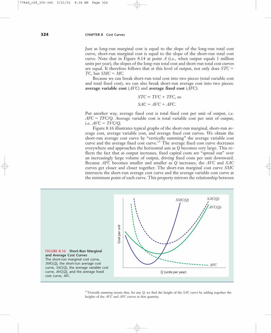
Just as long-run marginal cost is equal to the slope of the long-run total costcurve, short-run marginal cost is equal to the slope of the short-run total costcurve. Note that in Figure 8.14 at point A (i.e., when output equals 1 millionunits per year), the slopes of the long-run total cost and short-run total cost curvesare equal. It therefore follows that at this level of output, not only does STC �TC, but SMC � MC.
Because we can break short-run total cost into two pieces (total variable costand total fixed cost), we can also break short-run average cost into two pieces:average variable cost (AVC) and average fixed cost (AFC):
STC � TVC � TFC, so
SAC � AVC � AFC.
Put another way, average fixed cost is total fixed cost per unit of output, i.e.AFC � TFC/Q. Average variable cost is total variable cost per unit of output, i.e. AVC � TVC/Q.
Figure 8.16 illustrates typical graphs of the short-run marginal, short-run av-erage cost, average variable cost, and average fixed cost curves. We obtain theshort-run average cost curve by “vertically summing” the average variable costcurve and the average fixed cost curve.15 The average fixed cost curve decreaseseverywhere and approaches the horizontal axis as Q becomes very large. This re-flects the fact that as output increases, fixed capital costs are “spread out” over an increasingly large volume of output, driving fixed costs per unit downward.Because AFC becomes smaller and smaller as Q increases, the AVC and SACcurves get closer and closer together. The short-run marginal cost curve SMCintersects the short-run average cost curve and the average variable cost curve atthe minimum point of each curve. This property mirrors the relationship between
Cos
t per
uni
t
Q (units per year)
SMC(Q) SAC(Q)
AVC(Q)
AFC
FIGURE 8.16 Short-Run Marginal and Average Cost CurvesThe short-run marginal cost curve,SMC(Q), the short-run average costcurve, SAC(Q), the average variable costcurve, AVC(Q), and the average fixedcost curve, AFC.
15Vertically summing means that, for any Q, we find the height of the SAC curve by adding together theheights of the AVC and AFC curves at that quantity.
7784d_c08_300-345 5/21/01 8:38 AM Page 324
8.3 Short-Run Cost Curves 325
the long-run marginal and long-run average cost curves (and again reflects therelationship between the average and marginal measures of anything).
THE LONG-RUN AVERAGE COST CURVE AS AN ENVELOPE CURVE
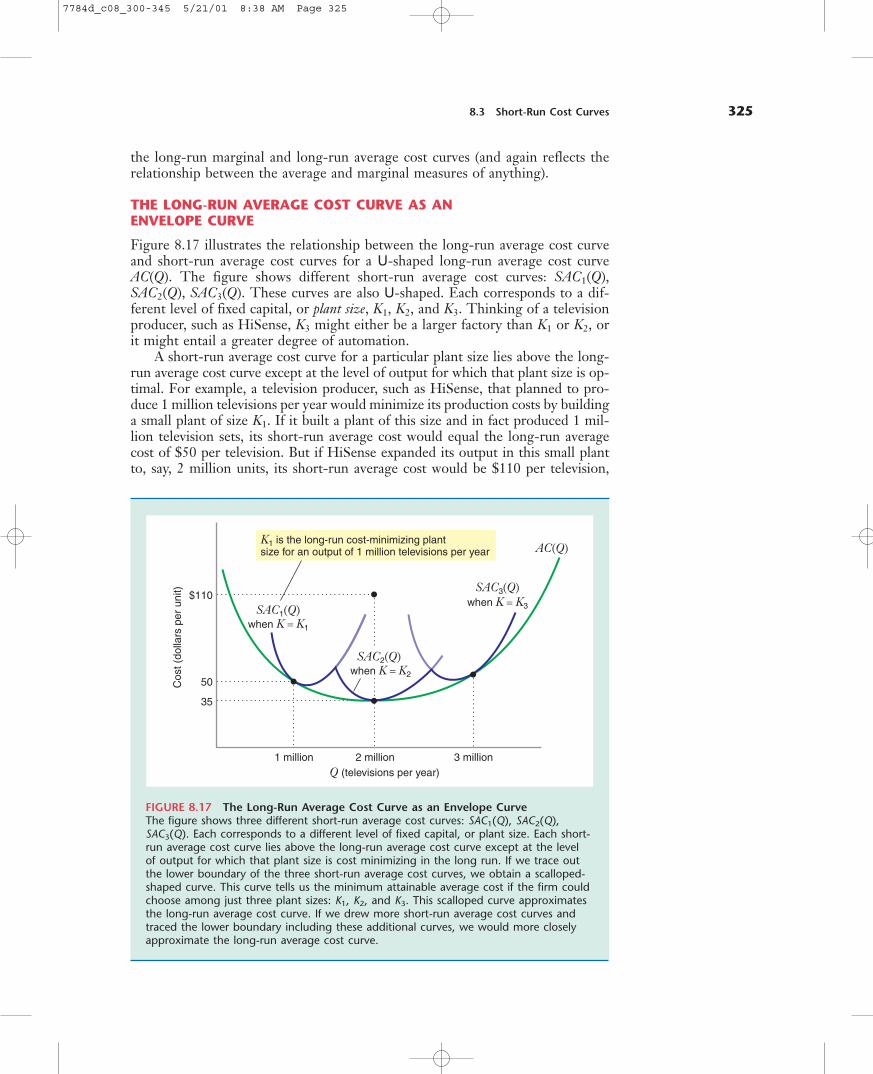
Figure 8.17 illustrates the relationship between the long-run average cost curveand short-run average cost curves for a U-shaped long-run average cost curveAC(Q). The figure shows different short-run average cost curves: SAC1(Q),SAC2(Q), SAC3(Q). These curves are also U-shaped. Each corresponds to a dif-ferent level of fixed capital, or plant size, K1, K2, and K3. Thinking of a televisionproducer, such as HiSense, K3 might either be a larger factory than K1 or K2, orit might entail a greater degree of automation.
A short-run average cost curve for a particular plant size lies above the long-run average cost curve except at the level of output for which that plant size is op-timal. For example, a television producer, such as HiSense, that planned to pro-duce 1 million televisions per year would minimize its production costs by buildinga small plant of size K1. If it built a plant of this size and in fact produced 1 mil-lion television sets, its short-run average cost would equal the long-run averagecost of $50 per television. But if HiSense expanded its output in this small plantto, say, 2 million units, its short-run average cost would be $110 per television,
Cos
t (do
llars
per
uni
t)
Q (televisions per year)1 million 2 million 3 million
K1 is the long-run cost-minimizing plantsize for an output of 1 million televisions per year
$110
50
35
SAC1(Q)
SAC2(Q)
AC(Q)
SAC3(Q)
when K = K2
when K = K3
when K = K1
FIGURE 8.17 The Long-Run Average Cost Curve as an Envelope CurveThe figure shows three different short-run average cost curves: SAC1(Q), SAC2(Q),SAC3(Q). Each corresponds to a different level of fixed capital, or plant size. Each short-run average cost curve lies above the long-run average cost curve except at the levelof output for which that plant size is cost minimizing in the long run. If we trace outthe lower boundary of the three short-run average cost curves, we obtain a scalloped-shaped curve. This curve tells us the minimum attainable average cost if the firm couldchoose among just three plant sizes: K1, K2, and K3. This scalloped curve approximatesthe long-run average cost curve. If we drew more short-run average cost curves andtraced the lower boundary including these additional curves, we would more closelyapproximate the long-run average cost curve.
7784d_c08_300-345 5/21/01 8:38 AM Page 325
326 CHAPTER 8 Cost Curves
E
S
D
LEARNING-BY-DOING EXERCISE 8.4
The Relationship Between Short-Run and Long-Run Average Cost Curves
Problem
(a) What is the long-run average cost curve for this production function?
Solution Recall from Learning-By-Doing Exercise 7.6 that the solution tothe long-run cost-minimization problem is
even though its long-run average cost at 2 million units is only $35 per television.This difference between the short-run average cost and the long-run average costillustrates a point we made in our earlier discussion of the relationship betweenthe short-run total cost and long-run total cost curve: you can never do better (i.e.,have lower total costs) in the short run than in the long run because in the longrun you can set all of your inputs to the levels that minimize total cost. (In prac-tice, the high unit cost that HiSense would incur from producing a relatively largeoutput in a small plant might reflect reductions in the marginal product of laborthat arise from crowding a large work force into a small plant.) In order to attainthe long-run average cost of $35 per television when producing 2 million televi-sions, HiSense would need to expand the size of its plant from K1 to K2.
If we traced the lower boundary of the three short-run average cost curves,we would obtain the dark “scalloped” curve in Figure 8.17. This curve tells us theminimum attainable average cost if the firm could choose only one of three plantsizes: K1, K2, and K3. The scalloped curve approximates the long-run average costcurve. If we drew more short-run average cost curves and traced the lower bound-ary including these additional curves, the resulting scalloped curve would be aneven better approximation to the long-run average cost curve. This argument tellsus that you can think of the long-run average cost curve as the “lower envelope”of an infinite number of short-run average cost curves. The long-run average costcurve is thus sometimes referred to as the envelope curve.
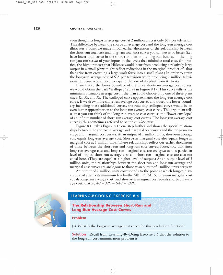
Figure 8.18 takes Figure 8.17 one step further and shows the special relation-ships between the short-run average and marginal cost curves and the long-run av-erage and marginal cost curves. At an output of 1 million units, short-run averagecost equals long-run average cost. Short-run marginal cost also equals long-runmarginal cost at 1 million units. These relationships reflect our earlier discussionsof those between the short-run and long-run cost curves. Note, too, that sincelong-run average cost and long-run marginal cost are not equal at this particularlevel of output, short-run average cost and short-run marginal cost are also notequal here. (They are equal at a higher level of output.) At an output level of 3million units, the relationships between the short-run and long-run average andmarginal cost curves are analogous to those at an output of 1 million units per year.
An output of 2 million units corresponds to the point at which long-run av-erage cost attains its minimum level—the MES. At MES, long-run marginal costequals long-run average cost, and short-run marginal cost equals short-run aver-age cost; that is, AC � MC � SAC � SMC.
7784d_c08_300-345 5/21/01 8:38 AM Page 326
8.3 Short-Run Cost Curves 327
Cos
t per
uni
t
Q (televisions per year)1 million 2 million = MES 3 million
SAC1(Q) SMC1(Q)
SAC2(Q)
SMC2(Q)
AC(Q)
MC(Q)
SAC3(Q)
SMC3(Q)
FIGURE 8.18 The Relationship Between the Long-Run Average and Marginal CostCurves and the Short-Run Average and Marginal Cost CurvesAt an output level of 1 million TVs per year (the output level for which plant size K1
solves the long-run cost-minimization problem), short-run average cost (SAC) equalslong-run average cost (AC(Q)). Short-run marginal cost (SMC) also equals long-runmarginal cost (MC(Q)) at 1 million units. Since AC(a) and MC(b) are not equal at thislevel of output, SAC and SMC are also not equal here. At an output level of 3 millionTVs per year, the relationships between the short-run and long-run average and mar-ginal cost functions are analogous to those at 1 million units. An output of 2 millionunits is where AC(Q) attains its minimum level; that is, it is the MES. At the MES,MC(Q) equals AC(Q), and thus SMC-SAC.
L � �Q8
�.
M � 2Q.
K � 2Q.
The input prices are w � 16, m � 1, and r � 2, so the long-run total costcurve is
TC(Q) � 16��Q8
�� � 1(2Q) � 2(2Q) � 8Q.
The long-run average cost curve is thus
AC(Q) � � � 8.8Q�Q
TC(Q)�
Q
7784d_c08_300-345 5/21/01 8:38 AM Page 327
328 CHAPTER 8 Cost Curves
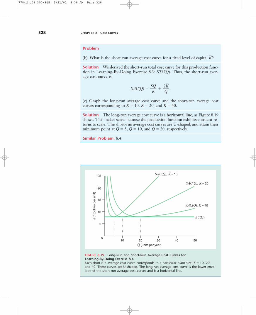
Problem
(b) What is the short-run average cost curve for a fixed level of capital K� ?
Solution We derived the short-run total cost curve for this production func-tion in Learning-By-Doing Exercise 8.3: STC(Q). Thus, the short-run aver-age cost curve is
SAC(Q) � � .
(c) Graph the long-run average cost curve and the short-run average costcurves corresponding to K� � 10, K� � 20, and K� � 40.
Solution The long-run average cost curve is a horizontal line, as Figure 8.19shows. This makes sense because the production function exhibits constant re-turns to scale. The short-run average cost curves are U-shaped, and attain theirminimum point at Q � 5, Q � 10, and Q � 20, respectively.
Similar Problem: 8.4
2K��Q
8Q�K
AC
(do
llars
per
uni
t)
Q (units per year)
10 30 4020 50
25
20
15
10
5
0
SAC(Q), K = 10
SAC(Q), K = 20
SAC(Q), K = 40
AC(Q)
FIGURE 8.19 Long-Run and Short-Run Average Cost Curves for Learning-By-Doing Exercise 8.4Each short-run average cost curve corresponds to a particular plant size: K � 10, 20,and 40. These curves are U-shaped. The long-run average cost curve is the lower enve-lope of the short-run average cost curves and is a horizontal line.
7784d_c08_300-345 5/21/01 8:38 AM Page 328
8.3 Short-Run Cost Curves 329
16The first part of this example box draws from “A Long Haul: America’s Railroads Struggle to Cap-ture Their Former Glory,” Wall Street Journal (December 5, 1997), p. A1 and A6.17R. R. Braeutigam, A. F. Daughety, and M. A. Turnquist, “A Firm Specific Analysis of Economies ofDensity in the U. S. Railroad Industry,” Journal of Industrial Economics 33 (September 1984); 3–20.18The identity of the firm remained anonymous to ensure the confidentiality of its data.19In this study, the railroad’s track mileage was adjusted to reflect changes in the quality of its trackover time.
EXAMPLE 8.5The Short-Run and Long-Run Cost Curves for an American Railroad Firm16
The 1990s were an interesting time for U.S. railroads. On the positive side, the rail-road industry was profitable, and the bankruptcies that had plagued the industryin the 1960s and 1970s were over. Some railroads, such as the Norfolk Southern,had become so optimistic about the future that they had begun ambitious invest-ments in new track. On the negative side, however, U.S. railroads had developeda generally poor reputation for service, particularly speed of delivery. On someroutes, shipping freight by train in the late 1990s took longer than it did thirty yearsearlier. Service became so bad that in 1997 Lionel, a company that makes toy trains,began shipping by truck rather than by rail. “We feel a little guilty forsaking ourbig brothers,” said Lionel President Gary Moreau, “But we have no choice.” Part ofthe problem, according to industry observers, arose because the railroad industrydownsized too much. During the 1980s and 1990s, U.S. railroads sold or aban-doned 55,000 miles of track. According to one expert, the railroads “. . . have toomuch freight trying to go over too little track.”
These concerns over the quality of rail service and how they relate to the amountof track a railroad employs might make you wonder how a railroad’s productioncosts depend on these factors. For example, would a railroad’s total variable costsgo down as it adds track? If so, at what rate? Would a faster service increase or de-crease a railroad’s cost of operation?
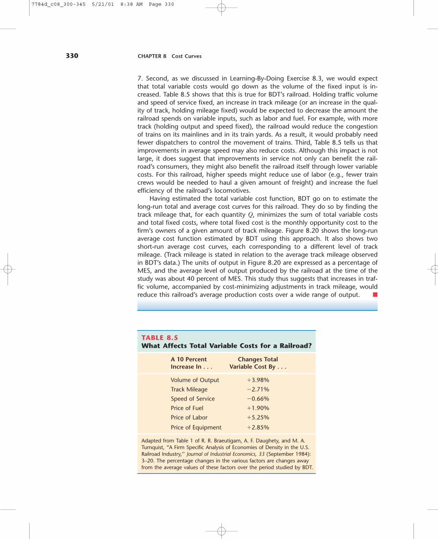
One way to study these questions would be to estimate the short-run and long-run cost curves for a railroad. In the 1980s, Ronald Braeutigam, Andrew Daughety,and Mark Turnquist (hereafter BDT) undertook such a study.17 With the coopera-tion of the management of a large American railroad firm, BDT obtained data oncosts of shipment, input prices (price of fuel, price of labor service), volume of out-put, and speed of service for this railroad.18 Using statistical techniques, they esti-mated a short-run total variable cost curve for the railroad. In the study, total vari-able cost is the sum of the railroad’s monthly costs for labor, fuel, maintenance, car,locomotive, and supplies.
Table 8.5 shows the impact on total variable costs of a hypothetical 10 percentincrease in (1) traffic volume (car-loads of freight per month); (2) the quantity of therailroad’s track (in miles); (3) speed of service (miles per day of loaded cars); and (4)the prices of labor, fuel, and equipment.19 You should think of track miles as a fixedinput, analogous to capital in our previous discussion. A railroad cannot instantlyvary the quantity or quality of its track to adjust to month-to-month variations inshipment volumes in the system and thus must regard track as a fixed input.
Table 8.5 contains several interesting findings. First, total variable cost increaseswith total output and with the prices of the railroad’s inputs. This is consistent withthe predictions of the theory you have been learning in this chapter and Chapter
7784d_c08_300-345 5/21/01 8:38 AM Page 329
330 CHAPTER 8 Cost Curves
7. Second, as we discussed in Learning-By-Doing Exercise 8.3, we would expectthat total variable costs would go down as the volume of the fixed input is in-creased. Table 8.5 shows that this is true for BDT’s railroad. Holding traffic volumeand speed of service fixed, an increase in track mileage (or an increase in the qual-ity of track, holding mileage fixed) would be expected to decrease the amount therailroad spends on variable inputs, such as labor and fuel. For example, with moretrack (holding output and speed fixed), the railroad would reduce the congestionof trains on its mainlines and in its train yards. As a result, it would probably needfewer dispatchers to control the movement of trains. Third, Table 8.5 tells us thatimprovements in average speed may also reduce costs. Although this impact is notlarge, it does suggest that improvements in service not only can benefit the rail-road’s consumers, they might also benefit the railroad itself through lower variablecosts. For this railroad, higher speeds might reduce use of labor (e.g., fewer traincrews would be needed to haul a given amount of freight) and increase the fuelefficiency of the railroad’s locomotives.
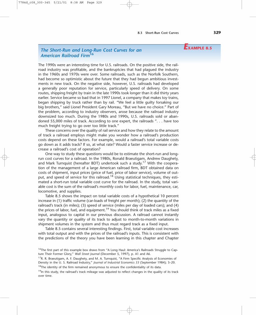
Having estimated the total variable cost function, BDT go on to estimate thelong-run total and average cost curves for this railroad. They do so by finding thetrack mileage that, for each quantity Q, minimizes the sum of total variable costsand total fixed costs, where total fixed cost is the monthly opportunity cost to thefirm’s owners of a given amount of track mileage. Figure 8.20 shows the long-runaverage cost function estimated by BDT using this approach. It also shows twoshort-run average cost curves, each corresponding to a different level of trackmileage. (Track mileage is stated in relation to the average track mileage observedin BDT’s data.) The units of output in Figure 8.20 are expressed as a percentage ofMES, and the average level of output produced by the railroad at the time of thestudy was about 40 percent of MES. This study thus suggests that increases in traf-fic volume, accompanied by cost-minimizing adjustments in track mileage, wouldreduce this railroad’s average production costs over a wide range of output. �
TABLE 8.5What Affects Total Variable Costs for a Railroad?
A 10 Percent Changes TotalIncrease In . . . Variable Cost By . . .
Volume of Output �3.98%
Track Mileage �2.71%
Speed of Service �0.66%
Price of Fuel �1.90%
Price of Labor �5.25%
Price of Equipment �2.85%
Adapted from Table 1 of R. R. Braeutigam, A. F. Daughety, and M. A.Turnquist, “A Firm Specific Analysis of Economies of Density in the U.S.Railroad Industry,’’ Journal of Industrial Economics, 33 (September 1984):3–20. The percentage changes in the various factors are changes awayfrom the average values of these factors over the period studied by BDT.
7784d_c08_300-345 5/21/01 8:38 AM Page 330
8.4 Special Topics in Cost 331
ECONOMIES OF SCOPE
This chapter has concentrated on cost curves for firms that produce just one prod-uct or service. In reality, though, many firms produce more than one product.For a firm that produces two products, total costs would depend on the quantityQ1 of the first product the firm makes and the quantity Q2 of the second prod-uct it makes. We will use the expression TC(Q1,Q2) to denote how the firm’s costsvary with Q1 and Q2. The total cost TC would be the minimized total cost of pro-ducing given quantities of the firm’s two products and would come from a cost-minimization problem that is analogous to the cost-minimization problem for asingle-product firm.
In some situations, efficiencies arise when a firm produces more than oneproduct. That is, a two-product firm may be able to manufacture and market itsproducts at a lower total cost than two single-product firms would incur whenproducing on a stand-alone basis. These efficiencies are called economies ofscope.
Specifically, economies of scope exist when the total cost of producing givenquantities of two goods in the same firm is less than the total cost of producingthose quantities in two single-product firms. Mathematically, this definition says
TC(Q1, Q2) � TC(Q1, 0) � TC(0, Q2). (8.4)
8.4SPECIALTOPICS INCOST
AC
(in
uni
ts o
f min
imum
AC
)
Q (in units of MES)
0.2 0.6 0.8 1.0 = MES0.4 1.2
1.0
0
SACSAC
AC(Q)
Track mileage 7.9 percent higher than average
Observed average output level
Track mileage 200 percent higher than average
FIGURE 8.20 Long-Run and Short-Run Average Cost Curves for a RailroadThe long-run and short-run average cost curves for the railroad studied by BDT are U-shaped. The two short-run average cost curves shown correspond to a different amountof track (expressed in relation to the average amount of track observed in the data). Thecost curves show that with a cost-minimizing adjustment in track size, this railroad coulddecrease its unit costs over a wide range of output above its current output level.
7784d_c08_300-345 5/21/01 8:38 AM Page 331
332 CHAPTER 8 Cost Curves
The zeros in the expressions on the right-hand side of equation (8.4) indicate thatthe single-product firms produce positive amounts of one good but none of theother. These are sometimes called the stand-alone costs of producing goods 1and 2.
Intuitively, the existence of economies of scope tells us that “variety” is moreefficient than “specialization.” We can develop an intuitive interpretation of thedefinition in 8.4 by rearranging terms as follows:
TC(Q1, Q2) � TC(Q1, 0) � TC(0, Q2) � TC(0, 0),
where TC(0, 0) � 0. That is, the total cost of producing zero quantities of bothproducts is zero. The left-hand side of this equation is the additional cost of pro-ducing Q2 units of product 2 when the firm is already producing Q1 units of product1. The right-hand side of this equation is the additional cost of producing Q2 whenthe firm does not produce Q1. Economies of scope exist if it is less costly for a firmto add a product to its product line given that it already produces another prod-uct. Economies of scope would exist, for example, if it is less costly for Coca-Cola to add a cherry-flavored soft drink to its product line than it would be fora new company starting from scratch.
Why would economies of scope arise? An important reason is a firm’s abil-ity to use a common input to make and sell more than one product. For exam-ple, BSkyB, the British satellite television company, can use the same satellite tobroadcast a news channel, several movie channels, several sports channels, andseveral general entertainment channels.20 Companies specializing in the broad-cast of a single channel would each need to have a satellite orbiting the Earth.BSkyB’s channels save hundreds of millions of dollars as compared to stand-alonechannels by sharing a common satellite. Another example is Eurotunnel, the 31-mile tunnel that runs underneath the English Channel between Calais, France,and Dover, Great Britain. The Eurotunnel accommodates both highway and railtraffic. Two separate tunnels, one for highway traffic and one for rail traffic, wouldhave been more expensive to construct and operate than a single tunnel that ac-commodates both forms of traffic.
20BSkyB is a subsidiary of Rupert Murdoch’s News Corporation.21This example is based on “Just Doing It: Nike Plans to Swoosh Into Sports Equipment But It’s aTough Game,” Wall Street Journal (January 6,1998), pp. A1 and A10.
EXAMPLE 8.6Nike Enters the Market for Sports Equipment 21
An important source of economies of scope is marketing. A company with a well-established brand name in one product line can sometimes introduce additionalproducts at a lower cost than a stand-alone company would be able to. This is be-cause when consumers are unsure about a product’s quality they often make in-ferences about its quality from the product’s brand name. This can give a firm withan established brand reputation an advantage over a stand-alone firm in introduc-
7784d_c08_300-345 5/21/01 8:38 AM Page 332
8.4 Special Topics in Cost 333
ing new products. Because of its brand reputation, an established firm would nothave to spend as much on advertising as the stand-alone firm to persuade con-sumers to try its product. This is an example of an economy of scope based on theability of all products in a firm’s product line to “share” the benefits of its estab-lished brand reputation.
A company with an extraordinary brand reputation is Nike. Nike’s “swoosh,”the symbol that appears on its athletic shoes and sports apparel, is one of the mostrecognizable marketing symbols of the modern age, and its slogan, “Just Do It,”has become ingrained in American popular culture. Nike’s slogan and swoosh areso recognizable that Nike can run television commercials that never mention itsname and be confidant that consumers will know whose products are being ad-vertised.
In the late 1990s, Nike turned its attention to the sports equipment market, in-troducing products such as hockey sticks and golf balls. Nike’s goal was to becomethe dominant firm in the $40 billion per year sports equipment market by 2005.This is a bold ambition. The sports equipment market is highly fragmented, and nosingle company has ever dominated the entire range of product categories thatNike intends to enter. In addition, while no one can deny Nike’s past success in theathletic shoe and sports apparel markets, producing a high-quality hockey stick oran innovative golf ball has little in common with making sneakers or jogging clothes.It therefore seems unlikely that Nike could attain economies of scope in manufac-turing or product design.
Nike hopes to achieve economies of scope in marketing. These economies ofscope would be based on its incredibly strong brand reputation, its close ties tosports equipment retailers, and its special relationships with professional athletessuch as Tiger Woods and Ken Griffey, Jr. Nike’s plan is to develop sports equipmentthat it can claim is innovative and then use its established brand reputation and itsties with the retail trade to convince consumers that its products are technically su-perior to existing products. If this plan works, Nike will be able to introduce its newproducts at far lower costs than a stand-alone company would incur to introduceotherwise identical products.
It will be interesting to see whether Nike succeeds. Economies of scope inmarketing can be powerful, but they also have their limits. A strong brand repu-tation can induce consumers to try a product once, but if it does not perform asexpected or if its quality is inferior, it may be difficult to penetrate the market orget repeat business. Nike’s preliminary forays into the sports equipment market il-lustrate this risk. In July 1997, Nike “rolled out” a new line of roller skates at theannual sports equipment trade show in Chicago. But when a group of skatersequipped with Nike skates rolled into the parking lot, the wheels on the skatesbegan to disintegrate! Quality problems have also arisen with a line of ice skatesthat Nike introduced several years ago. Jeremy Roenick, a star with the PhoenixCoyote’s NHL hockey team, turned down a six-figure endorsement deal with Nikebecause he felt the skates were poorly designed and did not fit properly. Rumorhas it that other hockey players who do have equipment deals with Nike use the products of competitors. According to one NHL equipment manager, “They’restill wearing the stuff they’ve been wearing for years. They just slap the swooshon it.” �
7784d_c08_300-345 5/21/01 8:38 AM Page 333
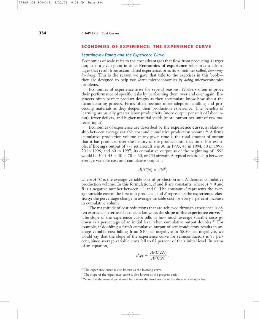
334 CHAPTER 8 Cost Curves
ECONOMIES OF EXPERIENCE: THE EXPERIENCE CURVE
Learning-by-Doing and the Experience CurveEconomies of scale refer to the cost advantages that flow from producing a largeroutput at a given point in time. Economies of experience refer to cost advan-tages that result from accumulated experience, or as its sometimes called, learning-by-doing. This is the reason we gave that title to the exercises in this book—they are designed to help you learn microeconomics by doing microeconomicsproblems.
Economies of experience arise for several reasons. Workers often improvetheir performance of specific tasks by performing them over and over again. En-gineers often perfect product designs as they accumulate know-how about themanufacturing process. Firms often become more adept at handling and pro-cessing materials as they deepen their production experience. The benefits oflearning are usually greater labor productivity (more output per unit of labor in-put), fewer defects, and higher material yields (more output per unit of raw ma-terial input).
Economies of experience are described by the experience curve, a relation-ship between average variable cost and cumulative production volume.22 A firm’scumulative production volume at any given time is the total amount of outputthat it has produced over the history of the product until that time. For exam-ple, if Boeing’s output of 777 jet aircraft was 30 in 1993, 45 in 1994, 50 in 1995,70 in 1996, and 60 in 1997, its cumulative output as of the beginning of 1998would be 30 � 45 � 50 � 70 � 60, or 255 aircraft. A typical relationship betweenaverage variable cost and cumulative output is
AVC(N) � ANB,
where AVC is the average variable cost of production and N denotes cumulativeproduction volume. In this formulation, A and B are constants, where A � 0 andB is a negative number between �1 and 0. The constant A represents the aver-age variable cost of the first unit produced, and B represents the experience elas-ticity: the percentage change in average variable cost for every 1 percent increasein cumulative volume.
The magnitude of cost reductions that are achieved through experience is of-ten expressed in terms of a concept known as the slope of the experience curve.23
The slope of the experience curve tells us how much average variable costs godown as a percentage of an initial level when cumulative output doubles.24 Forexample, if doubling a firm’s cumulative output of semiconductors results in av-erage variable cost falling from $10 per megabyte to $8.50 per megabyte, wewould say that the slope of the experience curve for semiconductors is 85 per-cent, since average variable costs fell to 85 percent of their initial level. In termsof an equation,
slope � .AVC(2N)��AVC(N)
22The experience curve is also known as the learning curve.23The slope of the experience curve is also known as the progress ratio.24Note that the term slope as used here is not the usual notion of the slope of a straight line.
7784d_c08_300-345 5/21/01 8:38 AM Page 334
8.4 Special Topics in Cost 335
The slope and the experience elasticity are systematically related. If the experi-ence elasticity is equal to B, the slope turns out to equal 2B. Figure 8.21 showsexperience curves with three different slopes: 90 percent, 80 percent, and 70 per-cent. The smaller the slope, the “steeper” the experience curve, (i.e., the morerapidly average variable costs fall as the firm accumulates experience). Note,though, that all three curves eventually flatten out. For example, beyond a vol-ume of N � 40, increments in cumulative experience have a small impact on av-erage variable costs, no matter what the slope of the experience curve is. At thispoint, most of the economies of experience are exhausted.
Experience curve slopes have been estimated for many different products.The median slope appears to be about 80 percent, implying that for the typicalfirm, each doubling of cumulative output reduces average variable costs to 80 per-cent of what they were before. Slopes vary from firm to firm and industry to in-dustry, however, so that the slope enjoyed by any one firm for any given pro-duction process generally falls between 70 and 90 percent and may be as low as60 percent or as high as 100 percent (i.e., no economies of experience).
Economies of Experience versus Economies of ScaleEconomies of experience differ from economies of scale. Economies of scale re-fer to the ability to perform activities at a lower unit cost when those activitiesare performed on a larger scale. Economies of experience refer to reductions inunit costs due to accumulating experience. Economies of scale may be substan-tial even when learning economies are minimal. This is likely to be the case inmature, capital-intensive production processes, such as aluminum can manufac-turing. Likewise, economies of experience may be substantial even wheneconomies of scale are minimal, as in complex labor-intensive activities such asthe production of handmade watches.
Firms that do not correctly distinguish between economies of scale and ex-perience might draw incorrect inferences about the benefits of size in a market.For example, if a firm has low average costs because of economies of scale,
N, cumulative output
AV
C (
dolla
rs/u
nit)
Slope = 90%
Slope = 80%
Slope = 70%
10 30 4020 50
1
0.8
0.6
0.4
0.2
1
FIGURE 8.21 Experience Curves With Different SlopesThe figure shows three experiencecurves, each with a different slope. Thesmaller the slope, the “steeper” the ex-perience curve, and the more rapidlyaverage variable costs fall as cumulativeexperience goes up. No matter whatthe slope, though, once cumulative ex-perience becomes sufficiently large (e.g.,N � 40), additional increments to expe-rience do not lower average variablecosts by much.
7784d_c08_300-345 5/21/01 8:38 AM Page 335
336 CHAPTER 8 Cost Curves
reductions in the current volume of production will increase unit costs. If the lowaverage costs are the result of cumulative experience, the firm may be able to cutback current production volumes without necessarily raising its average costs.
EXAMPLE 8.7The Experience Curve in the Production of EPROM Chips25
An interesting example of economies of experience occurs in the production ofsemiconductors, the memory chips that are used in personal computers, cellulartelephones, and electronic games. It is widely believed that the “yield” of semi-conductor chips—the ratio of usable chips total chips on a silicon wafer—goes upas a firm gains production experience.26 Silicon is an expensive raw material, andthe cost of a chip is primarily determined by how much silicon it uses. The rate atwhich yields go up with experience is thus important for a semiconductor manu-facturer to know.
Harald Gruber estimated the experience curve for a particular type of semi-conductor: erasable programmable read only memory (EPROM) chips. EPROM chipsare used to store program code for cellular phones, pagers, modems, video games,printers, and hard disk drives. An EPROM chip differs from the more common DRAMin that it is nonvolatile, which means that unlike a DRAM chip it retains its storeddata when the power is turned off. And in contrast to DRAM chips, which are pro-duced by large semiconductor firms such as Samsung and NEC, EPROM chips aregenerally produced by smaller firms, such as the Taiwanese firm Macronix.
Gruber recognized that other factors, such as economies of scale and memorycapacity, could influence the average cost of producing an EPROM chip. After con-trolling for these factors, Gruber found evidence of economies of experience in theproduction of EPROM chips. His estimate of the slope of the EPROM experiencecurve was 78 percent. Thus, by doubling its cumulative volume of chips, an EPROMproducer would expect its average variable costs to fall to 78 percent of their ini-tial level.
This is an interesting finding. The market for EPROM chips is smaller than mar-kets for other semiconductors, such as DRAMs, and as mentioned, most firms op-erate on a small scale. Moreover, new generations of EPROM chips are introducedfrequently, typically about once every 18 months. By contrast new generations ofDRAM chips were introduced about every 3 years during the 1980s and 1990s. Thissuggests that it is unlikely that an EPROM manufacturer will operate on the “flat”portion of the experience curve for long. By the time a firm starts to “move down”the experience curve, a new generation of chip will have come along. This, then,implies that a firm, such as Macronix, that can achieve a head start in bringing anew generation of EPROM chips to market, may achieve a significant cost advan-tage over slower competitors. �
25This example draws from H. Gruber, “The Learning Curve in the Production of SemiconductorMemory Chips,” Applied Economics, 24 (August 1992): 885–894.26A wafer is a slice of polycrystalline silicon. A chip producer will etch hundreds of circuits onto asingle wafer.
7784d_c08_300-345 5/21/01 8:38 AM Page 336
8.5 Estimating Cost Functions 337
Suppose you wanted to estimate how the total costs for a television producer, suchas HiSense, varied with the quantity of its output or the magnitude of its inputprices. To do this, you might want to estimate what economists call a total costfunction. A total cost function is a mathematical relationship that shows how to-tal costs vary with the factors that influence total costs. These factors are some-times called cost drivers. We’ve spent much of this chapter analyzing two keycost drivers: input prices and scale (volume of output). Our discussion in the pre-vious section suggests two other cost drivers that could also influence total costs:scope (variety of other goods produced by the firm) and cumulative experience.
How would you estimate a cost function? You would first need to gather data.When estimating cost functions, many economists use data from a cross-sectionof firms or plants at a particular point in time. A cross-section of television pro-ducers would consist of a sample of manufacturers or manufacturing facilities ina particular year, such as 2001. For each observation in your cross-section, youwould need information about total costs and cost drivers. The set of cost driversthat you include in your analysis is usually specific to what you are studying. Intelevision manufacturing, scale, cumulative experience, labor wages, materialsprices, and costs of capital would probably be important drivers for explainingthe behavior of average costs in the long run.
Having gathered data on total costs and cost drivers, you would then use sta-tistical techniques to construct an estimated total cost function. The most com-mon technique used by economists is multiple regression. The basic idea behindthis technique is to find a function that best fits our available data.
CONSTANT ELASTICITY COST FUNCTION
An important issue when you use multiple regression to estimate a cost functionis the functional form that relates the dependent variable of interest—in this case,total cost—to the independent variables of interest, such as output and inputprices. One common functional form is constant elasticity cost function. A con-stant elasticity cost function specifies a multiplicative relationship between totalcost, output, and input prices.
For a production process that involves two inputs, capital and labor, the con-stant elasticity long-run total cost function is
TC � aQbward,
where a, b, c, and d are constants. It is common to convert this into a relation-ship that is linear in the logs:
log TC � log a � b log Q � c log w � d log r,
and in this form, the constants a, b, c, and d can be estimated using multiple re-gression.
A useful feature of the constant elasticity specification is that the constant bis the output elasticity of total cost, discussed earlier. Analogously, the constantsc and d are the elasticities of long-run total cost with respect to the prices of labor and capital. These elasticities must be positive since, as we saw earlier, an increase in an input price will increase long-run total cost. We also learned
8.5ESTIMATINGCOSTFUNCTIONS*
7784d_c08_300-345 5/21/01 8:38 AM Page 337
338 CHAPTER 8 Cost Curves
earlier that a given percentage increase in w and r would have to increase long-run total cost by the same percentage amount. This implies that the constants cand d must add up to 1 (i.e., c � d � 1). Thus, for the estimated long-run totalcost function to be consistent with long-run cost minimization, this restrictionwould have to hold. This restriction can be readily incorporated into the multi-ple regression analysis.
TRANSLOG COST FUNCTION
The constant elasticity cost function does not allow for the possibility of averagecosts that first decrease in Q and then increase in Q (i.e., economies of scale, fol-lowed by diseconomies of scale). A cost function that allows for this possibility isthe translog cost function. A translog cost function postulates a quadratic rela-tionship between the log of total cost and the logs of input prices and output.The equation of the translog cost function is
log TC � b0 � b1 log Q � b2 log w � b3 log r � b4 (log Q)2 � (8.5)� b5(log w)2 � b6 (log r)2 � b7 (log w)(log r)� b8 (log w)(log Q) � b9 (log r)(log Q).
This formidable-looking expression turns out to have a lot of useful properties. Forone thing, it is often a good approximation of the cost functions that come fromjust about any production function. Thus, if (as is often the case) we don’t knowthe exact functional form of the production function, the translog would be a goodchoice for the functional form of the cost function. In addition, the average costfunction for the translog total cost function can be U-shaped. Thus, it allows forboth economies of scale and diseconomies of scale. Note, too, that if b5 � b6 � b7� b8 � b9 � 0, the translog cost function reduces to the constant elasticity costfunction. Thus, the constant elasticity cost function is a special case of the translogcost function. Finally, the restrictions on the constants that make a percentage in-crease in all input prices lead to the same percentage increase in long-run total cost(so that the cost function is consistent with long-run cost minimization) are notdifficult to state. For the cost function in (8.5) they are as follows:
b2 � b3 � 1
b5 � b6 � b7 � 0
b8 � b9 � 0
CHAPTER SUMMARY
• The long-run total cost curve shows how the mini-mized level of total cost varies with the quantity of out-put. LBD 8.1
• An increase in factor prices rotates the long-run to-tal cost curve upward through the point Q � 0.
• Long-run average cost is the firm’s cost per unit ofoutput. It equals total cost divided by output. LBD 8.2
• Long-run marginal cost curve is the rate of change oflong-run total cost with respect to output. LBD 8.2
• Economies of scale describe a situation in whichlong-run average cost decreases in output. Econ-omies of scale arise because of the physical propertiesof processing units, specialization of labor, and indivisibilities.
7784d_c08_300-345 5/21/01 8:38 AM Page 338

• Diseconomies of scale describe a situation in whichlong-run average cost increases in output. A key sourceof diseconomies of scale are managerial diseconomies.
• The minimum efficient scale (MES) is the smallestquantity at which the long-run average cost curve attainsits minimum.
• The output elasticity of total cost is the percentagechange in total cost per 1 percent change in output.
• The short-run total cost curve tells us the minimizedtotal cost as a function of output, input prices, and thelevel of the fixed input(s). LBD 8.3
• Short-run total cost is the sum of two components:total variable cost and total fixed cost.
• Corresponding to the short-run total cost curve arethe short-run average cost and short-run marginal costcurves. Short-run average cost is the sum of average vari-able cost and average fixed cost.
• The long-run average cost curve is the lower enve-lope of short-run average cost curves. LBD 8.4
• Economies of scope exist when it is less costly to pro-duce given quantities of two products with one firm thanit is with two firms, each specializing in the productionof a single product.
• Economies of experience exist when average vari-able cost decreases with cumulative production volume.The experience curve tells us how average variable costsare affected by changes in cumulative production volume.
• Cost drivers are factors such as output or the pricesof inputs that influence the level of costs.
• Two common functional forms that are used for real-world estimation of cost functions are the constant elas-ticity cost function, and the translog cost function.
Review Questions 339
1. What is the relationship between the solution tothe firm’s long-run cost minimization problem and thelong-run total cost curve?
2. Explain why an increase in the price of an input musttypically cause an increase in the long-run total cost ofproducing any particular level of output.
3. If the price of labor increases by 20 percent, but allother input prices remain the same, would the long-runtotal cost at a particular output level go up by more than20 percent, less than 20 percent, or exactly 20 percent?If the prices of all inputs went up by 20 percent, wouldlong-run total cost go up by more than 20 percent, lessthan 20 percent, or exactly 20 percent?
4. How would an increase in the price of labor shiftthe long-run average cost curve?
5. a) If the average cost curve is increasing, must theaverage cost curve always lie above the marginal costcurve? Why or why not?b) If the marginal cost curve is increasing, must the av-erage cost curve always lie above the marginal cost curve?Why or why not?
6. Sketch the long-run marginal cost curve for the“flat-bottomed” long-run average cost curve shown inFigure 8.11.
7. Could the output elasticity of total cost ever be neg-ative?
8. Explain why the short-run marginal cost curve mustintersect the average variable cost curve at the minimumpoint of the average variable cost curve.
9. Suppose the graph of the average variable cost curveis flat. What shape would the short-run marginal costcurve be? What shape would the short-run average costcurve be?
10. Suppose that the minimum level of short-run av-erage cost was the same for every possible plant size.What would that tell you about the shapes of the long-run average and long-run marginal cost curves?
11. What is the difference between economies of scopeand economies of scale? Is it possible for a two-productfirm to enjoy economies of scope but not economies ofscale? Is it possible for a firm to have economies of scalebut not economies of scope?
12. What is an experience curve? What is the differ-ence between economies of experience and economies ofscale?
REVIEW QUESTIONS
7784d_c08_300-345 5/21/01 8:38 AM Page 339
1. A firm produces a product with labor and capital,and its production function is described by
Q � LK.
The marginal products associated with this productionfunction are
MPL � K.
MPK � L.
Suppose that the price of labor equals 2, and the priceof capital equals 1. Derive the equations for the long-run total cost curve and the long-run average cost curve.
2. A firm’s long-run total cost curve is
TC(Q) � 1000Q � 30Q2 � Q3.
Derive the expression for the corresponding long-runaverage cost curve and then sketch it. At what quantityis minimum efficient scale?
3. Consider a production function of two inputs: laborand capital, given by
Q � [L�12�
� K �12�]2.
The marginal products associated with this productionfunction are as follows:
MPL � [L�12�
� K �12�] L
��12�.
MPK � [L�12�
� K �12�] K
��12�.
Let w � 2 and r � 1.
a) Suppose the firm is required to produce Q units ofoutput. Show how the cost-minimizing quantity of labordepends on the quantity Q. Show how the cost-minimizing quantity of capital depends on the quantity Q.b) Find the equation of the firm’s long-run total costcurve.c) Find the equation of the firm’s long-run average costcurve.d) Find the solution to the firm’s short-run cost-minimization problem when capital is fixed at a quantityof 10 units (i.e., K� � 9).e) Find the short-run total cost curve, and graph it alongwith the long-run total cost curve.f ) Find the associated short-run average cost curve.
4. Consider a production function of three inputs, labor, capital, and materials given by
Q � LKM
The marginal products associated with this productionfunction are as follows:
MPL � KM
MPK � LM
MPM � LK
Let w � 5, r � 1, and m � 2, where m is the price perunit of materials.
a) Suppose that the firm is required to produce Q unitsof output. Show how the cost-minimizing quantity of la-bor depends on the quantity Q. Show how the cost-min-imizing quantity of capital depends on the quantity Q.Show how the cost-minimizing quantity of materials de-pends on the quantity Q.b) Find the equation of the firm’s long-run total costcurve.c) Find the equation of the firm’s long-run average costcurve.d) Suppose that the firm is required to produce Q units ofoutput, but that its capital is fixed at a quantity of 50 units(i.e., K� � 50). Show how the cost-minimizing quantity oflabor depends on the quantity Q. Show how the cost-min-imizing quantity of materials depends on the quantity Q.e) Find the equation of the short-run total cost curvewhen capital is fixed at a quantity of 50 units (i.e., K� � 50)and graph it along with the long-run total cost curve.f ) Find the equation of the associated short-run averagecost curve.
5. A short-run total cost curve is given by the equation
STC(Q) � 1000 � 50Q2.
Derive expressions for and then sketch the correspon-ding short-run average cost, average variable cost, andaverage fixed cost curve.
6. A producer of hard disk drives has a short-run totalcost curve given by
STC(Q) � K� � �QK�
2
� .
Within the same set of axes, sketch a graph of the short-run average cost curves for three different plant sizes: K� � 10, K� � 20, and K� � 30. Based on this graph, whatis shape of the long-run average cost curve?
7. Figure 8.17 shows that the short-run marginal costcurve may lie above the long-run marginal cost curve.Yet, in the long run, the quantities of all inputs are vari-able, whereas in the short run, the quantities of just someof the inputs are variable. Given that, why isn’t short-run marginal cost less than long-run marginal cost forall output levels?
PROBLEMS
340 CHAPTER 8 Cost Curves
7784d_c08_300-345 5/21/01 8:38 AM Page 340
8. Suppose that the total cost of providing satellite tele-vision services is as follows
TC(Q1, Q2) �0 if Q1 � 0 and Q2 � 0.1000 � 2Q1 � 3Q2 otherwise,
where Q1 and Q2 are the number of households that sub-scribe to a sports and movie channel, respectively. Doesthe provision of satellite television services exhibiteconomies of scope?
9. A researcher has claimed to have estimated a long-run total cost function for the production of automo-biles. His estimate is that
TC(Q, w, r) � 100w��12� r �
12�Q3,
where w and r are the prices of labor and capital. Is thisa valid cost function—that is, it consistent with long-runcost minimization by the firm? Why or why not?
APPENDIX: Shephard’s Lemma and Duality 341
WHAT IS SHEPHARD’S LEMMA?
Let’s compare our calculations in Learning-By-Doing Exercise 7.4 in Chapter 7and Learning-By-Doing Exercise 8.1 in this chapter. Both pertain to the pro-duction function Q � 50K �
12�L�
12�. Our input demand functions were
K*(Q, w, r) � �5Q0� ��
wr���
12�
.
L*(Q, w, r) � �5Q0� ��
wr���
12�
.
Our long-run total cost function was
TC(Q, w, r) � Q.
Let’s see how the long-run total cost function varies with respect to the price oflabor w, holding Q and r fixed.
� �5Q0� ��
wr���
12�
� L*(Q, w, r). (A8.1)
The rate of change of long-run total cost with respect to the price of labor is equal to thelabor demand function. Similarly,
� �5Q0� ��
wr���
12�
� K*(Q, w, r). (A8.2)
The rate of change of long-run total cost with respect to the price of capital is equal tothe capital demand function.
The relationships summarized in equations (A8.1) and (A8.2) are no coinci-dence. They reflect a general relationship between the long-run total cost function
∂TC(Q, w, r)��
∂r
∂TC(Q, w, r)��
∂w
w�12�r �
12�
�25
APPENDIX: Shephard’s Lemma and Duality
7784d_c08_300-345 5/21/01 8:38 AM Page 341
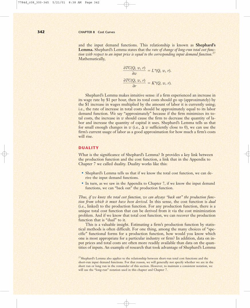
and the input demand functions. This relationship is known as Shephard’sLemma. Shephard’s Lemma states that the rate of change of long-run total cost func-tion with respect to an input price is equal to the corresponding input demand function.27
Mathematically,
� L*(Q, w, r).
� K*(Q, w, r).
Shephard’s Lemma makes intuitive sense: if a firm experienced an increase inits wage rate by $1 per hour, then its total costs should go up (approximately) bythe $1 increase in wages multiplied by the amount of labor it is currently using;i.e., the rate of increase in total costs should be approximately equal to its labordemand function. We say “approximately” because if the firm minimizes its to-tal costs, the increase in w should cause the firm to decrease the quantity of la-bor and increase the quantity of capital it uses. Shephard’s Lemma tells us thatfor small enough changes in w (i.e., � w sufficiently close to 0), we can use thefirm’s current usage of labor as a good approximation for how much a firm’s costswill rise.
DUALITY
What is the significance of Shephard’s Lemma? It provides a key link betweenthe production function and the cost function, a link that in the Appendix toChapter 7 we called duality. Duality works like this:
• Shephard’s Lemma tells us that if we know the total cost function, we can de-rive the input demand functions.
• In turn, as we saw in the Appendix to Chapter 7, if we know the input demandfunctions, we can “back out” the production function.
Thus, if we know the total cost function, we can always “back out” the production func-tion from which it must have been derived. In this sense, the cost function is dual(i.e., linked) to the production function. For any production function, there is aunique total cost function that can be derived from it via the cost minimizationproblem. And if we know that total cost function, we can recover the productionfunction that is “dual” to it.
This is a valuable insight. Estimating a firm’s production function by statis-tical methods is often difficult. For one thing, among the many choices of “spe-cific” functional forms for a production function, how would you know whichone is most appropriate for a particular industry or firm? In addition, data on in-put prices and total costs are often more readily available than data on the quan-tities of inputs. An example of research that took advantage of Shephard’s Lemma
∂TC(Q, w, r)��
∂r
∂TC(Q, w, r)��
∂w
342 CHAPTER 8 Cost Curves
27Shephard’s Lemma also applies to the relationship between short-run total cost functions and theshort-run input demand functions. For that reason, we will generally not specify whether we are in theshort run or long run in the remainder of this section. However, to maintain a consistent notation, wewill use the “long-run” notation used in this chapter and Chapter 7.
7784d_c08_300-345 5/21/01 8:38 AM Page 342
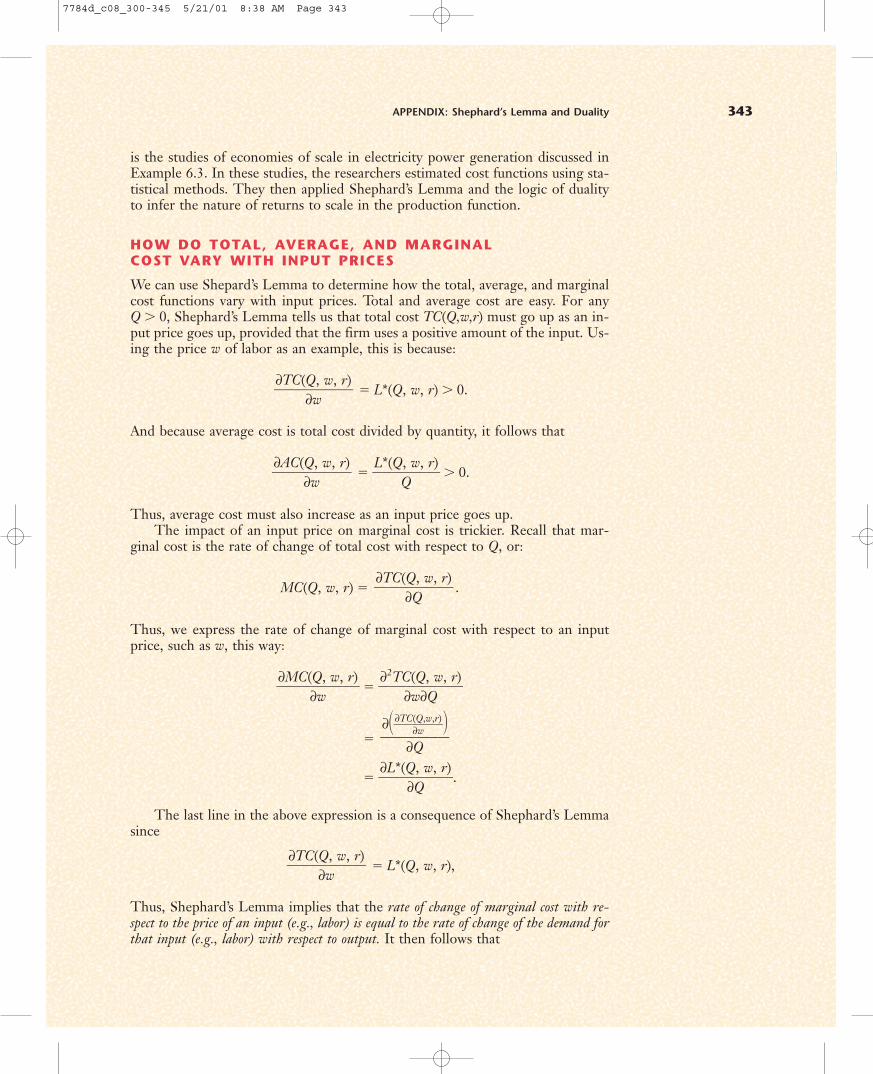
APPENDIX: Shephard’s Lemma and Duality 343
is the studies of economies of scale in electricity power generation discussed inExample 6.3. In these studies, the researchers estimated cost functions using sta-tistical methods. They then applied Shephard’s Lemma and the logic of dualityto infer the nature of returns to scale in the production function.
HOW DO TOTAL, AVERAGE, AND MARGINAL COST VARY WITH INPUT PRICES
We can use Shepard’s Lemma to determine how the total, average, and marginalcost functions vary with input prices. Total and average cost are easy. For any Q � 0, Shephard’s Lemma tells us that total cost TC(Q,w,r) must go up as an in-put price goes up, provided that the firm uses a positive amount of the input. Us-ing the price w of labor as an example, this is because:
� L*(Q, w, r) � 0.
And because average cost is total cost divided by quantity, it follows that
� �L*(Q
Q, w, r)� � 0.
Thus, average cost must also increase as an input price goes up.The impact of an input price on marginal cost is trickier. Recall that mar-
ginal cost is the rate of change of total cost with respect to Q, or:
MC(Q, w, r) � .
Thus, we express the rate of change of marginal cost with respect to an inputprice, such as w, this way:
�∂MC(
∂Qw, w, r)� ��
∂2TC∂w(Q
∂,Qw, r)
�
�
� �∂L*(Q
∂Q, w, r)�.
The last line in the above expression is a consequence of Shephard’s Lemmasince
� L*(Q, w, r),
Thus, Shephard’s Lemma implies that the rate of change of marginal cost with re-spect to the price of an input (e.g., labor) is equal to the rate of change of the demand forthat input (e.g., labor) with respect to output. It then follows that
∂TC(Q, w, r)��
∂w
∂��∂TC∂(Qw
,w,r)��
��∂Q
∂TC(Q, w, r)��
∂Q
∂AC(Q, w, r)��
∂w
∂TC(Q, w, r)��
∂w
7784d_c08_300-345 5/21/01 8:38 AM Page 343
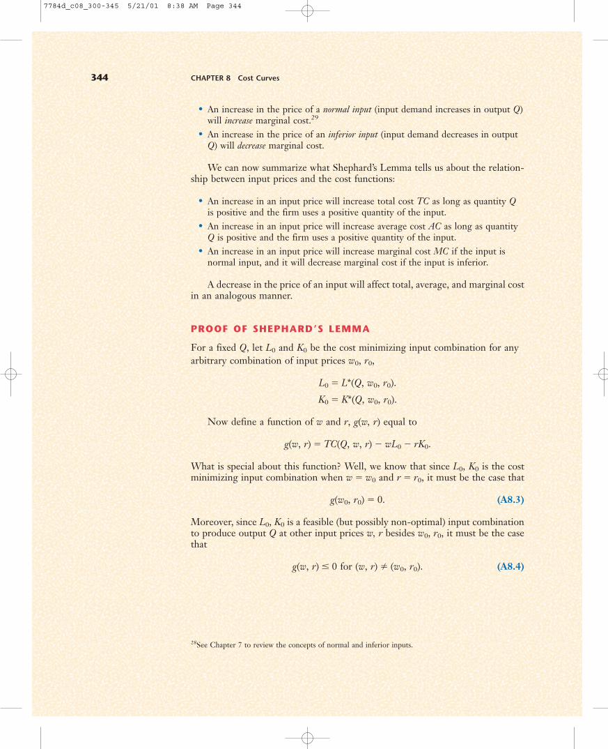
• An increase in the price of a normal input (input demand increases in output Q)will increase marginal cost.29
• An increase in the price of an inferior input (input demand decreases in outputQ) will decrease marginal cost.
We can now summarize what Shephard’s Lemma tells us about the relation-ship between input prices and the cost functions:
• An increase in an input price will increase total cost TC as long as quantity Qis positive and the firm uses a positive quantity of the input.
• An increase in an input price will increase average cost AC as long as quantityQ is positive and the firm uses a positive quantity of the input.
• An increase in an input price will increase marginal cost MC if the input isnormal input, and it will decrease marginal cost if the input is inferior.
A decrease in the price of an input will affect total, average, and marginal costin an analogous manner.
PROOF OF SHEPHARD’S LEMMA
For a fixed Q, let L0 and K0 be the cost minimizing input combination for anyarbitrary combination of input prices w0, r0,
L0 � L*(Q, w0, r0).
K0 � K*(Q, w0, r0).
Now define a function of w and r, g(w, r) equal to
g(w, r) � TC(Q, w, r) � wL0 � rK0.
What is special about this function? Well, we know that since L0, K0 is the costminimizing input combination when w � w0 and r � r0, it must be the case that
g(w0, r0) � 0. (A8.3)
Moreover, since L0, K0 is a feasible (but possibly non-optimal) input combinationto produce output Q at other input prices w, r besides w0, r0, it must be the casethat
g(w, r) � 0 for (w, r) � (w0, r0). (A8.4)
344 CHAPTER 8 Cost Curves
28See Chapter 7 to review the concepts of normal and inferior inputs.
7784d_c08_300-345 5/21/01 8:38 AM Page 344
Conditions (A8.3) and (A8.4) imply that the function g(w, r) attains its maximumwhen w � w0 and r � r0. Hence, at these points, its partial derivatives with re-spect to w and r must be zero:
�∂g(w
∂w0, r0)� � 0 → �
∂TC(Q∂,ww0, r0)�� L0. (A8.5)
�∂g(w
∂0
r, r0)� � 0 → �
∂TC(Q∂,rw0, r0)�� K0. (A8.6)
But since L0 � L*(Q, w0, r0) and K0 � K*(Q, w0, r0), (A8.5) and (A8.6) imply
�∂TC(Q
∂,ww0, r0)�� L*(Q, w0, r0). (A8.7)
�∂TC(Q
∂,rw0, r0)�� K*(Q, w0, r0). (A8.8)
Since w0, r0 is an arbitrary combination of input prices, conditions (A8.7) and(A8.8) hold for any pair of input prices, and this is exactly what we wanted toshow to prove Shephard’s Lemma.
Appendix: Proof of Shephard’s Lemma 345
7784d_c08_300-345 5/21/01 8:39 AM Page 345