cosmological consistency relations - home page | iris ... · cosmological consistency relations...
TRANSCRIPT
Scuola Internazionale Superiore di Studi AvanzatiArea of Physics
Ph.D. in Astroparticle Physics
Cosmological Consistency Relations
Candidate: Supervisor:
Marko Simonovic Paolo Creminelli
Thesis submitted in partial fulfillment of the requirements
for the degree of Doctor Philosophiae
Academic Year 2013/2014


Acknowledgements
At the beginning of this thesis I would like to thank many people who made this work possible.
First of all I would like to thank Paolo for his guidance, patience and support over the last
three years. It was a pleasure and privilege to work with him and I am forever indebted to
him for all the effort he put in bringing me to this point. He was a great teacher and friend.
During my PhD I had a chance to collaborate with many excellent people from whom I
learned a lot. I would like to thank Razieh Emami, Jerome Gleyzes, Austin Joyce, Justin
Khoury, Diana Lopez Nacir, Jorge Norena, Manuel Pena, Ashley Perko, Leonardo Senatore,
Gabriele Trevisan, Filippo Vernizzi and Matias Zaldarriaga for many fruitful collaborations.
It was a great experience to work with them.
I would particularly like to thank Nima Arkani-Hamed, Daniel Baumann, Diego Blas,
Emanuele Castorina, Kurt Hinterbichler, Lam Hui, Mehrdad Mirbabayi, Marcello Musso,
Alberto Nicolis, Aseem Paranjape, Marco Peloso, Massimo Pietroni, Roman Scoccimarro,
Emiliano Sefusatti, Uros Seljak, Ravi Sheth and Enrico Trincherini for many useful discussions
from which I learned a lot and that influenced my work significantly.
At the end I would like to thank Daniel Baumann and Massimo Pietroni for carefully
reading my thesis and sending back many useful comments that significantly improved its
quality.

Contents
1 Introduction 1
1.1 Correlation Functions and Symmetries . . . . . . . . . . . . . . . . . . . . . . 3
1.2 Consistency Relations . . . . . . . . . . . . . . . . . . . . . . . . . . . . . . . 6
2 Theory of Cosmological Perturbations 9
2.1 Relativistic Perturbation Theory . . . . . . . . . . . . . . . . . . . . . . . . . 9
2.1.1 Background Evolution . . . . . . . . . . . . . . . . . . . . . . . . . . . 10
2.1.2 Perturbed Einstein Equations . . . . . . . . . . . . . . . . . . . . . . . 11
2.1.3 Newtonian Gauge . . . . . . . . . . . . . . . . . . . . . . . . . . . . . . 12
2.2 Cosmological Perturbations from Inflation . . . . . . . . . . . . . . . . . . . . 13
2.2.1 Inflation . . . . . . . . . . . . . . . . . . . . . . . . . . . . . . . . . . . 13
2.2.2 The Power Spectrum . . . . . . . . . . . . . . . . . . . . . . . . . . . . 14
2.2.3 Non-Gaussianities . . . . . . . . . . . . . . . . . . . . . . . . . . . . . . 18
2.3 Perturbation Theory in the Late Universe . . . . . . . . . . . . . . . . . . . . 20
2.3.1 Fluid Description of Dark Matter . . . . . . . . . . . . . . . . . . . . . 21
2.3.2 Linear Perturbation Theory . . . . . . . . . . . . . . . . . . . . . . . . 22
2.3.3 Non-linear Perturbation Theory . . . . . . . . . . . . . . . . . . . . . . 23
3 Construction of Adiabatic Modes 26
3.1 Newtonian Gauge . . . . . . . . . . . . . . . . . . . . . . . . . . . . . . . . . . 27
3.1.1 Weinberg’s Construction . . . . . . . . . . . . . . . . . . . . . . . . . . 27
3.1.2 Homogeneous Gradients . . . . . . . . . . . . . . . . . . . . . . . . . . 29
3.1.3 Including Short Modes . . . . . . . . . . . . . . . . . . . . . . . . . . . 32
3.2 ζ-Gauge . . . . . . . . . . . . . . . . . . . . . . . . . . . . . . . . . . . . . . . 34
3.2.1 Scalar Modes . . . . . . . . . . . . . . . . . . . . . . . . . . . . . . . . 34
3.2.2 Tensor Modes . . . . . . . . . . . . . . . . . . . . . . . . . . . . . . . . 36
3.3 Checks . . . . . . . . . . . . . . . . . . . . . . . . . . . . . . . . . . . . . . . . 37
3.3.1 The Second Order Metric in a Matter Dominated universe . . . . . . . 37
3.3.2 The Squeezed Limit of δ(2) in a Matter Dominated Unverse . . . . . . . 40
3.3.3 The Cubic Action for Single-field Inflation . . . . . . . . . . . . . . . . 43
i

4 Inflationary Consistency Relations 46
4.1 Consistency Relations for Scalars . . . . . . . . . . . . . . . . . . . . . . . . . 46
4.1.1 Maldacena’s Consistency Relation . . . . . . . . . . . . . . . . . . . . . 48
4.1.2 Conformal Consistency Relations . . . . . . . . . . . . . . . . . . . . . 49
4.1.3 Comments . . . . . . . . . . . . . . . . . . . . . . . . . . . . . . . . . . 54
4.1.4 Checks . . . . . . . . . . . . . . . . . . . . . . . . . . . . . . . . . . . . 56
4.2 Consistency Relations for Gravitational Waves . . . . . . . . . . . . . . . . . . 61
4.2.1 Derivation . . . . . . . . . . . . . . . . . . . . . . . . . . . . . . . . . . 61
4.2.2 Checks . . . . . . . . . . . . . . . . . . . . . . . . . . . . . . . . . . . . 62
4.3 Soft internal lines . . . . . . . . . . . . . . . . . . . . . . . . . . . . . . . . . . 63
4.4 Going to Higher Order in q . . . . . . . . . . . . . . . . . . . . . . . . . . . . . 64
4.4.1 A Heuristic Argument . . . . . . . . . . . . . . . . . . . . . . . . . . . 65
4.4.2 From ζ-gauge to a Curved FRW Universe . . . . . . . . . . . . . . . . 68
4.4.3 Checks . . . . . . . . . . . . . . . . . . . . . . . . . . . . . . . . . . . . 70
4.5 Multiple Soft Limits . . . . . . . . . . . . . . . . . . . . . . . . . . . . . . . . 72
4.5.1 Zeroth Order in Gradients . . . . . . . . . . . . . . . . . . . . . . . . . 73
4.5.2 First Order in Gradients . . . . . . . . . . . . . . . . . . . . . . . . . . 75
4.5.3 Second Order in Gradients . . . . . . . . . . . . . . . . . . . . . . . . . 76
4.5.4 Checks . . . . . . . . . . . . . . . . . . . . . . . . . . . . . . . . . . . . 78
4.6 Consistency Relations as Ward Identities . . . . . . . . . . . . . . . . . . . . . 79
4.6.1 Decoupling Limit . . . . . . . . . . . . . . . . . . . . . . . . . . . . . . 80
4.6.2 Ward Identities . . . . . . . . . . . . . . . . . . . . . . . . . . . . . . . 83
5 Consistency Relations of Large Scale Structure 85
5.1 Relativistic Consistency Relations of LSS . . . . . . . . . . . . . . . . . . . . . 86
5.1.1 Derivation . . . . . . . . . . . . . . . . . . . . . . . . . . . . . . . . . . 87
5.1.2 Comments . . . . . . . . . . . . . . . . . . . . . . . . . . . . . . . . . . 92
5.1.3 Checks . . . . . . . . . . . . . . . . . . . . . . . . . . . . . . . . . . . . 94
5.2 Non-relativistic Limit and Resummation . . . . . . . . . . . . . . . . . . . . . 95
5.2.1 Resumming the long mode . . . . . . . . . . . . . . . . . . . . . . . . . 97
5.2.2 Several soft legs . . . . . . . . . . . . . . . . . . . . . . . . . . . . . . . 99
5.2.3 Soft Loops . . . . . . . . . . . . . . . . . . . . . . . . . . . . . . . . . . 101
5.2.4 Soft internal lines . . . . . . . . . . . . . . . . . . . . . . . . . . . . . . 102
5.3 Consistency Relations in Redshift Space . . . . . . . . . . . . . . . . . . . . . 104
5.3.1 Derivation . . . . . . . . . . . . . . . . . . . . . . . . . . . . . . . . . . 105
5.3.2 Checks . . . . . . . . . . . . . . . . . . . . . . . . . . . . . . . . . . . . 107
5.4 Violation of the Equivalence Principle . . . . . . . . . . . . . . . . . . . . . . . 108
5.4.1 Modifications of gravity and EP violation . . . . . . . . . . . . . . . . . 110
5.4.2 Signal to noise for the bispectrum . . . . . . . . . . . . . . . . . . . . . 114
5.5 Other Applications . . . . . . . . . . . . . . . . . . . . . . . . . . . . . . . . . 119
ii

6 Conclusions and Outlook 121
A Correlation Functions in Inflation 123
A.1 Single-field Slow-roll Inflation . . . . . . . . . . . . . . . . . . . . . . . . . . . 123
A.1.1 Three-point Correlation Functions . . . . . . . . . . . . . . . . . . . . . 123
A.1.2 Four-point Correlation Functions . . . . . . . . . . . . . . . . . . . . . 124
A.2 Models with Reduced Speed of Sound . . . . . . . . . . . . . . . . . . . . . . . 124
A.3 Resonant non-Gaussianities . . . . . . . . . . . . . . . . . . . . . . . . . . . . 126
A.4 Khronon Inflation . . . . . . . . . . . . . . . . . . . . . . . . . . . . . . . . . . 127
A.4.1 The Power Spectrum . . . . . . . . . . . . . . . . . . . . . . . . . . . . 127
A.4.2 The 3-point function . . . . . . . . . . . . . . . . . . . . . . . . . . . . 128
B Derivation of the Consistency Relation for Gravitational Waves 130
C An Example of the Equivalence Principle Violation 133
iii

Chapter 1
Introduction
In the last several decades we witnessed a tremendous progress in cosmology. From a theory
with mainly qualitative ideas about the expanding universe originated from a state with high
density and temperature (Hot Big Bang cosmological model), cosmology rapidly evolved to
a science in which the composition and the evolution of the universe are known well enough
to make very detailed predictions for a large number of observables on many different scales
and different redshifts. Many of these predictions can be tested nowadays in observations to
a percent accuracy, and planned future experiments will push the limits even further. This
progress brought to us some of the most important and exciting discoveries in the history of
science, helping us to understand in detail the history of our universe over the whole 13.7
billion years of its evolution.
It is fair to say that the era of precision cosmology started with the first detection of
anisotropies in the Cosmic Microwave Background (CMB) by the COBE satellite [1]. A
series of ground-based and balloon-borne experiments improved the measurements of the
power spectrum of temperature fluctuations in the CMB in the following decade and lead
to the discovery of acoustic peaks which provided an independent measurement of cosmo-
logical parameters (see for example [2, 3]). Observations strongly supported the existence of
non-baryonic dark matter and confirmed the existence of dark energy discovered around the
same time in the observations of supernovae at high redshift [4, 5]. The characteristic shape
of the power spectrum of temperature fluctuations with acoustic peaks, measured flatness of
the universe and scale invariance of the power spectrum of primordial fluctuations were all in
agreement with the inflationary predictions, severely constraining alternative mechanisms for
generation of the CMB anisotropies. At the same time, the estimates of cosmological param-
eters from the CMB were in a good agreement with local measurements (see for example [6]),
indicating that we have a consistent picture of the universe. Although all these steps brought
groundbreaking discoveries, the potential of the CMB as the leading probe of cosmology was
still to be fully explored.
The new era started with new satellites. The first to fly was WMAP. Apart from signifi-
cantly improving the precision of measurements of the composition of the universe, WMAP
also brought for the first time interesting constraints on the initial conditions, ruling out some
1

inflationary models [7]. It delivered tight constraints on non-Gaussianities, that shrank the
parameter space for inflation more than ever [8, 9, 10]. The latest results from measurements
of the CMB temperature anisotropies came form Planck [11, 12, 13]. Probably the most
important single result is confirmation of a small negative tilt of the power spectrum of initial
curvature perturbations, predicted by the simplest inflationary models. The scale invariant
power spectrum was ruled out for the first time in a single experiment with more than 5σ
[12]. On the other hand, with new, much tighter constraints on non-Gaussianities we are
entering in the interesting regime of parameters where we can make some general statements
about the nature of inflation. All these results can still improve after the data release form
polarisation measurements by the Planck collaboration.
Although for some observations (like temperature fluctuations in the CMB) we are reaching
the cosmic variance limited precision, the CMB still remains a gold mine of data. In particular,
there is a lot of space for improvement in measurements of polarisation. The most interesting
observable are the so called B-modes of the CMB polarisation, because in the absence of vector
modes they can be induced only by tensor perturbations [14, 15]. Therefore, a detection of
B-modes (on top of the signal coming form CMB lensing) would be a detection of primordial
gravitational waves and confirmation of the inflationary paradigm. The first encouraging steps
were made recently. The first evidence for B-modes induced by CMB lensing was found in
[16, 17]. After that, the BICEP collaboration announced the first direct detection of B-modes
at a degree scale, with amplitude much higher than the leasing contribution [18]. Although
there is an ongoing debate about whether this signal is of cosmological origin or not [19, 20],
it is certain that a new era in observational cosmology is opened and we will have much more
data coming in the following years.
In the meantime a big progress has been made in extracting the cosmological parameters
from observations of Large Scale Structure (LSS). A series of galaxy surveys (for example
[21, 22, 23]) allowed us to learn a lot about structure formation and late evolution of the
universe. A lot of work has been done in order to understand how to use this growing amount
of data to learn about the statistics of the initial conditions, constrain possible modifications
of gravity, study the properties of dark energy, explore galaxy formation etc. Despite huge
complexity due to non-linear gravitational collapse and complicated baryonic physics involved
in galaxy formation, a big advantage of LSS is that it, in principle, contains much more
information than the CMB. The reason for this is simply that the amount of modes available
is much larger. At the moment, some of the parameters obtained form LSS surveys are already
competitive with CMB results. With future experiments, the LSS will become the leading
probe of cosmology (see for example [24]).
Combining all the data mentioned above allowed us to measure the cosmological parame-
ters better than ever and establish ΛCDM as the standard model of cosmology. All observa-
tional evidence tell us that our universe is homogeneous and isotropic on large scales, spatially
flat, with around 5% of baryons, around 27% of cold dark matter (CDM) and dominated by
the cosmological constant Λ that causes the accelerated expansion. The initial curvature per-
turbations have a scale-invariant power spectrum, they are highly Gaussian and perturbations
2

are adiabatic, all in agreement with predictions of the simplest models of inflation. So far, in
observations, we do not see any statistically significant disagreement with the predictions of
ΛCDM model. Still, many questions remain without answers. For example, just to mention
some of them, we still do not know what is the statistic of primordial perturbations, what is
the nature of dark energy or whether or not general relativity (GR) is modified on cosmolog-
ical scales. For some of these questions we may find the answers already in some of the next
generation experiments.
It is important to stress that almost all this huge progress has been made measuring dif-
ferent correlation functions. Although the study of the background evolution was important
to establish the hot Big Bang model, only with the development of perturbation theory and
measurements of the correlation functions of cosmological perturbations it became possible
to make a crucial improvement in our ability to learn about the universe. There are many
different observables, from fluctuations in the CMB (including temperature and polarization),
neutral hydrogen at high redshifts, Lyman-alpha forest, to galaxy surveys in our local cosmo-
logical environment. All these observables are sensitive to different scales at different epochs
of the universe and to many different processes that are involved in the evolution of cosmo-
logical perturbations. Therefore, one of the most important goals of theoretical cosmology is
to find reliable methods to calculate different correlation functions for a given cosmological
model. Over the past several decades a lot of progress has been made, from calculations
of inflationary predictions, linear perturbation theory and CMB physics, to some techniques
that capture non-linear effects and gravitational collapse in the late universe—all in order
to better understand the evolution of cosmological perturbations. Cosmological consistency
relations, as general theorems about correlation functions, are an important part of this effort.
1.1 Correlation Functions and Symmetries
One of the most powerful tools that we have at hand in the study of cosmological correlation
functions are symmetries. They were used to construct a very useful and general effective
field theory approach to single-field [25] and multi-field inflation [26], some of the dark energy
models [27, 28] and large scale structure [29, 30, 31, 32, 33]. They also play an important
role in the study of non-Gaussianities, independently of that whether they are imposed on
the background [34], perturbations [35] or non-linearly realised [25, 36], just to mention some
examples. The consistency relations, that are the main subject of this thesis, also came from
studying the symmetries of cosmological perturbations. In all these cases, like in QFT, the
symmetries help us to construct the theories, find general statements, constrain solutions or
access the non-perturbative regime.
As an illustration, let us take a look at the example of isometries of de Sitter space, which
is a good approximation for the space-time during inflation. Let us also, for the time being,
focus on the case of a test field ϕ in de Sitter1. For example, using only de Sitter isometries
1This is relevant in some inflationary models where the curvature perturbation dominantly come form a
3

we can show that the power spectrum of ϕ is scale-invariant. Indeed, de Sitter space-time is
described by the following metric
ds2 =1
H2η2
(−dη2 + d~x2
), (1.1)
with a constant Hubble parameter H (η is conformal time). Being a maximally symmetric
space-time, de Sitter has 10 isometries. Six of them are spatial translations and rotations,
and they constrain the correlation functions in a trivial way. One of the remaining isometries
is the rescaling of coordinates η → λη and ~x → λ~x. Given this symmetry in real space, the
2-point function of ϕ in momentum space has to satisfy the following property
〈ϕ~k1/λ(λη)ϕ~k2/λ
(λη)〉 = λ6〈ϕ~k1(η)ϕ~k2
(η)〉 . (1.2)
This constraint, after imposing the translational invariance, immediately tells us that
〈ϕ~k1(η)ϕ~k2
(η)〉 = (2π)3δ(~k1 + ~k2)1
k31
F (k1η) , (1.3)
where F (x) is some unknown function. However, we are usually interested in the late-time
limit η → 0, in which the unknown part becomes just a constant F (0). In this way, without
specifying any details of the theory, we were able to show that the two-point function indeed
must be scale invariant.
Inspired by this example, we can take a look at the remaining three isometries of de Sitter
space. They are parametrized by an infinitesimal parameter ~b
η → η − 2η(~b · ~x) , xi → xi − bi(−η2 + ~x2) + 2xi(~b · ~x) . (1.4)
Do these isometries constrain the correlation functions in a similar way as dilations? For
a test field in de Sitter this must be the case, because the correlation functions depend on
de Sitter invariant distances and therefore must be invariant under (1.4). Indeed, this can
be explicitly checked for several situations that are relevant for inflation (the consequences of
these isometries were first studied in [39]). For example, the correlation functions of gravitons
are expected to be invariant under (1.4), because gravitons behave just as a test field in the
inflating background [40]. It is interesting to notice that in the late time limit the isometries
(1.4) act on the spatial coordinates as the special conformal transformation [39, 40]. In this
sense, we can say that the graviton three-point functions must be conformally invariant [40].
This is a very strong statement, that immediately tells us that the shape of the three-point
function for gravitons is fixed up to a normalisation, independently on the interactions. The
same applies to correlation functions of curvature perturbations, in inflationary models where
the curvature perturbations are generated by some spectator field [41]. Also in this case the
shape of the three-point function is fixed by conformal invariance and the scaling dimension of
light test field like the curvaton [37, 38].
4
the field (which depends on its mass). In all these examples, for a massless field ϕ, invariance
under (1.4) in momentum space implies
bi ·n∑a=1
[6∂kai − kai~∂2
ka + 2(~ka · ~∂ka)∂kai)]〈ϕ~k1
ϕ~k2. . . ϕ~kn〉
′ = 0 , (1.5)
where the prime on the correlation functions indicates that the momentum conserving delta
function has been removed.
Naturally, one is immediately tempted to think that these conclusions can be easily gen-
eralised to any inflationary model, given that quantum fluctuations that eventually produce
curvature perturbations live in an approximately de Sitter background during inflation. How-
ever, it is straightforward to check that although approximately scale-invariant, the correlation
functions of curvature perturbations in single-field inflation are not invariant under confor-
mal transformations. The resolution to this apparent paradox is very simple. Unlike in the
case of test fields, in single-field inflation the curvature perturbations are generated from the
fluctuations of the inflaton around some time-dependent background. This time-dependent
background breaks the isometries2 of de Sitter spontaneously, and the correlation functions
of perturbations do not depend on de Sitter invariant distances.
Let us take a more detailed look at what happens. We can parametrize the background as
we like, and let us say that φ = t+π. Now the isometries of de Sitter are non-linearly realised
on π. For dilation t → t + C, and consequently π → π − C. However, an approximate shift
symmetry is typically assumed in inflation. It is for this reason that the correlation functions
are scale invariant. Dilation is spontaneously broken, but in combination with shift symmetry
it is recovered. Indeed, the amount of breaking is proportional to the amount of breaking of
the shift symmetry, which is related to the slow-roll parameters. On the other hand, nothing
similar happens for conformal transformations. They are broken and there is no symmetry
that help them to be restored3.
However, this does not mean that one cannot say anything about the consequences of
de Sitter isometries. The symmetry is still there in the original Lagrangian—on the level of
perturbations it is only non-linearly realised. The situation is the same as in QFT, where
usually some internal symmetry is spontaneously broken. It is well known that in these
kind of theories one can derive Ward identities that relate correlation functions of different
order. Although the spontaneous breaking of space-time symmetries is somewhat different
from internal symmetries4, similar identities can be written for the inflationary correlation
functions as well. They have the following form
〈ζ~qζ~k1. . . ζ~kn〉
′q→0 = −P (q)
[3(n− 1) +
∑a
~ka · ~∂ka +1
2qiδ
(n)
Ki +O(q/k)2
]〈ζ~k1
. . . ζ~kn〉′ , (1.6)
2It breaks isometries that are related to time. Spatial translations and rotations remain linearly realised.3For more details, see the discussion in Section 4.6.4For example the number of Goldstone bosons is not equal to the number of broken generators, for more
details see [42].
5
where δ(n)
Ki is a differential operator in (1.5). These equations that relate the squeezed limit of
the correlation functions with lower order correlation functions are called consistency relations.
1.2 Consistency Relations
So far we used arguments based on de Sitter isometries to claim that there are some non-
trivial relations between inflationary correlation functions of different order called consistency
relations. However, during inflation the metric fluctuates as well. Including gravity is never
easy, but it turns out that the consistency relations remain valid in all single-field models,
even when the coupling with gravity is taken into account. In order to prove this stronger
statement we cannot use the isometries of de Sitter anymore. Instead we need a different kind
of insight.
The insight is that in single-field models5 the long-wavelength mode is locally indistinguish-
able from a coordinate transformation [43, 44, 45]. Indeed, if we have only one dynamical
degree of freedom during inflation, then all parts of the universe follow the same classical
history and quantum fluctuations of the inflaton are locally equivalent to a small shift of this
classical history in time. This shift in time is then equivalent to an additional expansion that
is equivalent to a simple rescaling of coordinates. Of course, this is true once the long mode
crosses the horizon, because after that it becomes frozen and remains constant. For short
modes its effect is not physical because it is just a classical background whose effect can be
removed just by a rescaling of coordinates. Notice that this argument is independent on the
details of interactions, the form of the kinetic term, slow-roll assumptions or any other details
of the theory [45]. We will make this discussion a bit more formal in Chapter 3.
The other way to see the same thing is to say that in single-field models one can connect
two different solutions of Einstein equations, one with short modes and a long mode and one
with the same short modes but without the long mode, just using the change of coordinates.
This is the heart of the consistency relations, because it allows us to find a relation between
the correlation functions of different order. On one side we have a correlation function with
one long mode and n short modes. In momentum space this means that the momentum of
the long mode is much smaller than all the others, and we get the left hand side of (1.6). On
the other side is a variation of the n-point function under the change of coordinates which in
momentum space becomes the right hand side of (1.6).
At zeroth order in ~q (the first term on the right hand side of (1.6)) the consistency relations
were first shown to hold for the three-point functions in single-field slow-roll inflation [43]. It
was later proven that they hold for any n-point function in any model of single-field inflation
[45] (for a proof in the framework of the EFT of inflation see [46]). Let us immediately stress
the most important consequence of the consistency relations. Given the approximate scale
invariance of the two-point function, they imply that the local non-Gaussianities must be
small in any single-field model of inflation. In other words, any detection of f loc.NL 1 would
5Here we assume that the inflaton is on the dynamical attractor and standard Bunch-Davies vacuum.
6

rule out all single-field models. For this reason Maldacena’s consistency relation is one of the
most important theorems about non-Gaussianities.
The behaviour of the three-point function in the squeezed limit was further investigated
in [47] where it was shown that the corrections to the leading result linear in ~q vanish. This
is not the case in general for the squeezed limit of an n-point function. The form of the
term linear in ~q was first discussed in [48]. It is the second term on the right hand side in
(1.6). Given that the long mode at this order in gradients is equivalent to a special conformal
transformation of spatial coordinates, the result is dubbed conformal consistency relation.
Since then there was a lot of progress in understanding the origin of the consistency relations
in different ways. They were derived as Ward identities [49, 50, 51], using the wavefunciton
of the universe [52], as Slavnov-Taylor identities for diffeomorphism invariance [53, 54], using
operator product expansion techniques [55, 56] and the holographic description of inflation
[57, 58]. We will discuss some of these approaches in Chapter 4. As a final comment let us
say that, although we are not going to consider it in this theses, the same arguments can
be applied even in models that are alternatives to inflation. One example of this kind is the
conformal mechanism [59, 60, 61, 62]. The consistency relations for this kind of models were
derived in [63].
Although the consistency relations were originally derived for inflation, it is possible to
use the same arguments in the late universe. As long as the long adiabatic mode is outside
the dynamical horizon (the sound horizon) it can be seen locally as a gauge transformation
(assuming single-field inflation). For example, using this property one can calculate ana-
lytically the squeezed limit of the bispectrum of temperature fluctuations in the CMB [64].
This calculation connects the inflationary consistency relations with observables, and shows
precisely in what sense the single-field models predict small local non-Gaussianities.
This is not the end of consistency relation because we can keep applying the same logic even
at later times. After recombination the sound horizon practically shrinks to zero. Therefore,
all the modes that enter the horizon afterwards are outside the sound horizon and the same
arguments as in inflation apply to them too. Locally, these long adiabatic modes are just a
coordinate transformations. This insight leads to the consistency relations of LSS that were
a subject of an intense study recently. Using a different approach they were first derived
in Newtonian limit in [65, 66] and then following the arguments described here generalised
in [67] to the relativistic result and including baryons. An incomplete set of references that
explored and extended these results include [68, 69, 70, 71, 72, 73, 74, 75]. As we will show in
Chapter 5, the consistency relations of LSS have the same form as the consistency relations
for inflation. Here we quote just the result in the non-relativistic limit [65, 66, 69]
〈δ~q(η) δ~k1(η1) · · · δ~kn(ηn)〉′q→0 = −Pδ(q, η)
∑a
Dδ(ηa)
Dδ(η)
~q · ~kaq2〈δ~k1
(η1) · · · δ~kn(ηn)〉′ . (1.7)
where δ is the density contrast and Dδ(η) the growth function of perturbations.
What makes the consistency relations of LSS very interesting is that they are non-
perturbative result and they hold independently of baryon physics and bias. Indeed, as
7

we will see in Chapter 5, we can write them down for correlation functions of galaxies directly
in redshift space. Notice that, although we cannot calculate non-pertubatively any of these
correlation functions, we can still prove that the relation (1.7) holds. It is also important
to stress that they are valid even for the long modes that are inside the Hubble radius and
therefore observable. However, for the observationally most interesting case of equal-time
correlation functions, the right hand side of the consistency relation vanishes. The situation
is somewhat similar to what happens in inflation, where due to approximate scale invariance
the right hand side of Maldacena’s consistency relation is unobservable. Still, we can use
this to our advantage. Instead of trying to confirm them, we can search for violations of the
consistency relations. Indeed, if any of the assumptions entering the derivation of the consis-
tency relations is violated, then the right hand side of (1.7) will not be zero. Apart from the
assumption of single-field inflation, the other crucial ingredient that we need for eq. (1.7) to
hold is the equivalence principle (EP). Therefore, what we learn from the consistency relations
of LSS is that any violation of the EP on cosmological scales would induce the 1/q divergence
in the squeezed limit of the three-point function. This provides a new, model independent
test of general relativity on cosmological scales. We will explore the ability of future surveys
to constrain the EP violations in Chapter 5.
To conclude, given the importance and complexity of cosmological correlation functions
described at the beginning of this introduction, the consistency relations are interesting as
a rare example of non-perturbative and model-independent statements that one can make.
They are derived form the fact that, in any single-field model and assuming GR, ever since
the long mode leaves the horizon and remains outside the sound horizon its effect on the short
modes is equivalent to a change of coordinates and therefore unphysical. The future probes
will have a potential to measure the correlation functions with increasing precision. As we
pointed out, if the consistency relations are falsified in future observations, it would be a sign
of either a violation of the EP on cosmological scales or multifield inflation, or both.
8

Chapter 2
Theory of Cosmological Perturbations
The theory of cosmological perturbations is in the heart of modern cosmology. According
to the standard ΛCDM model, inhomogeneities that we observe in the universe come from
quantum fluctuations stretched by inflation. These fluctuations eventually come back inside
the horizon and evolve during different epochs of the history of the universe. We can see them
as small fluctuations of the temperature in the CMB on the one side and as fluctuations in
the number density of galaxies on the other. The best way to characterise these perturbations
is through their correlation functions. Given complicated interactions over a very long period
of time, these correlation functions are very sensitive to cosmological parameters. It is for
this reason that the study of cosmological perturbations is crucial for our ability to compare
theories and observations and find the correct model for our universe.
The purpose of this Chapter is not to go through all details of the evolution of cosmological
perturbations. We will just fix the notation and give an overview of the main results that we
are going to use in the following chapters. In particular, our focus will be on calculations of
correlation functions that are necessary for many checks of the consistency relations, both for
inflation and LSS. Many details of these calculations that we are going to skip can be found
in many excellent articles, reviews, lecture notes and textbooks and we will refer the reader
to some of them when needed.
2.1 Relativistic Perturbation Theory
At early times and large distances compared to the curvature scale, relativistic effects cannot
be neglected. Therefore, for a complete description of cosmological fluctuations one necessarily
needs a perturbation theory that is compatible with general relativity. We focus on it in this
Section. Our main goal is to introduce the perturbed Einstein equations in Newtonian gauge
that we will need in Chapter 3. Many more details about perturbation theory can be found
in textbooks on cosmology (see for example [76, 77, 78]).
9

2.1.1 Background Evolution
In order to introduce some notation and set the stage for the study of perturbations, we begin
by a brief review of the background evolution of the Universe. All observational evidence that
we have tells us that the Universe is homogeneous and isotropic on cosmological scales. This
large amount of symmetry simplifies its description significantly. Averaged over space, all
relevant quantities such as density, temperature, pressure and others can depend only on
time.
Indeed, assuming that the spatial curvature is zero1, the line element takes the following
simple form
ds2 = −dt2 + a(t)2d~x2 . (2.1)
This is the well known Friedmann-Robertson-Walker (FRW) metric. In this metric a(t) is
some time dependent function called scale factor. The scale factor contains information about
the expansion history of the Universe and it can be determined once the composition and the
initial conditions are known. Before we move to the dynamics, let us introduce conformal
time η that we will use frequently. Conformal time is defined in the following way
η =
∫dt
a(t), (2.2)
such that the FRW metric in new coordinates is conformal to Minkowski space-time
ds2 = a2(η)(−dη2 + d~x2
). (2.3)
These coordinates are particularly useful for the study of the causal structure of the FRW
space-time. For the rest of the thesis, dots will denote the standard time derivative with
respect to t, while primes will denote derivatives with respect to conformal time, ′ ≡ ∂η.
In order to describe the dynamics of the expansion we have to use the Einstein equations.
With ansatz (2.1) the Einstein equations give(a
a
)2
≡ H2 =8πG
3ρ ,
a
a= −4πG
3(ρ+ 3p) . (2.4)
These are the famous Friedmann equations, that describe the evolution of the scale factor.
The quantity H ≡ a/a is Hubble expansion rate. Written in terms of conformal time these
equations become (a′
a
)2
≡ H2 =8πG
3a2ρ ,
a′′
a=
4πG
3a2(ρ− 3p) . (2.5)
Notice that on the right hand side of these equations we have the total energy density ρ and
pressure p of a fluid that fills the universe. They come from the energy-momentum tensor
1This is one of the inflationary predictions and it is in a perfect agreement with observations [11]. We will
always assume zero spatial curvature throughout the thesis.
10

on the right hand side of Einstein equations. It is a good approximation to use the energy-
momentum of a perfect fluid, which in a frame comoving with the fluid has the following
simple form T µν = diag(ρ,−p,−p,−p).Notice that equations (2.4) can be combined to get
ρ+ 3H(ρ+ p) = 0 . (2.6)
This is the continuity equation and it can be obtained from the conservation of the energy-
momentum tensor too. Finally, in order to solve Friedmann equations we need to specify the
equation of state of the fluid. We can use the following parametrization p = wρ in which
case, for constant w, the continuity equation gives
ρ ∼ a−3(1+w) . (2.7)
Now it is straightforward to find the solution for the scale factor. It is given by
a(t) ∼ t2
3(1+w) , w 6= −1 . (2.8)
Using w = 0 for ordinary matter or w = 1/3 for radiation, we recover the well known results
in cases of matter and radiation dominated universe. In the case w = −1 the energy density
is constant and the universe expands exponentially a ∼ eHt. This is for example the case
during inflation.
2.1.2 Perturbed Einstein Equations
The universe is homogeneous and isotropic only on cosmological scales and the Friedmann
equations can describe well only the background evolution where all quantities are averaged
in space. In order to study small perturbations around this background we have to allow for
space and time dependence and the Einstein equations become more complicated. Once the
background is subtracted we are left with
δGµν = 8πGδTµν . (2.9)
If the perturbations are small, we can do a perturbative expansion on both sides. For most
of the purposes in cosmology it is enough to keep only the linear terms.
The main problem with relativistic perturbation theory is gauge redundancy in GR. The
freedom to choose the coordinates means that there is no clear distinction between what we
call background and what are perturbations. Of course, physical quantities cannot depend
on this choice and this is why only gauge invariant observables have physical sense. The way
one typically deals with these issues is to fix some gauge, do the calculation and then make
the connection to the observables. This situation is familiar form classical electrodynamics,
which is a gauge theory too.
Let us take a closer look on the left hand side of eq. (2.9). In general the metric fluctuations
can be written in the following way
ds2 = −(1 + 2Φ)dt2 + 2aBidxidt+ a2 [(1− 2Ψ)δij + Eij] dxidxj . (2.10)
11

The perturbations Φ and Ψ are scalars and Bi and Eij can be decomposed into scalar, vector
and tensor parts2. Notice that, as in any gauge theory, the number of components in the
metric is always larger than the number of actual physical degrees of freedom. It is also
important to stress that the scalar components of the metric transform under the change of
coordinates and therefore they are not physical quantities.
On the right hand side of eq. (2.9) we can write the fluctuations in energy-momentum
tensor like
T 00 = −(ρ+ δρ) , (2.11)
T 0i = (ρ+ p)vi , (2.12)
T ij = δij(p+ δp) + Πij , (2.13)
where bar denotes background quantities and Πij is the anisotropic stress.
Let us at the end mention two important gauge invariant quantities that we will use later
in the thesis. One is the curvature perturbation on uniform-density hypersurfaces
ζ ≡ −Ψ− H˙ρδρ . (2.14)
The other one is the comoving curvature perturbation
R ≡ Ψ− H
ρ+ pv , (2.15)
where v is the velocity potential vi = ∂iv. One can explicitly check that these two quantities
remain invariant under the change of coordinates.
2.1.3 Newtonian Gauge
As we said, the way to deal with gauge redundancy is to fix the gauge and then do the calcu-
lation. In this section we show how the perturbed Einstein equations look like in Newtonian
gauge. Newtonian gauge is defined by B = E = 0, such that the metric (2.10) takes the
following form
ds2 = a2(η)[−(1 + 2Φ)dη2 + (1− 2Ψ)d~x2
]. (2.16)
Notice that this metric has a familiar form of a metric in the weak gravitational field. This
gauge is very convenient for LSS calculations, and it is intuitive because in the non-relativistic
limit Φ becomes the gravitational potential.
Once we fix the gauge, it is straightforward to calculate the variation of the Einstein
tensor. The perturbed Einstein equations in Newtonian gauge give
∇2Ψ− 2H(Ψ′ +HΦ) = 4πGa2ρ δ , (2.17)
∂i(Ψ′ +HΦ) = (H2 −H′)∂iv , (2.18)
Ψ′′ +H(Φ′ + 2Ψ′) + (2H′ +H2)Φ− 1
3∇2(Ψ− Φ) = 4πGa2δp , (2.19)
∂i∂j(Ψ− Φ) = 8πGΠij . (2.20)
2Vector modes are not produced during inflation and we will neglect them in the rest of the discussion.
12

In the absence of vector and tensor perturbation we can write the anisotropic stress as Πij =
∂i∂jδσ. We are going to use these equations in Chapter 3.
2.2 Cosmological Perturbations from Inflation
Inflation is a leading paradigm for describing the early universe. Originally, inflation was
introduced as a solution for three famous problems of the standard hot Big Bang cosmology:
horizon problem, flatness problem and magnetic monopoles problem (for example see [79,
80, 81, 82, 83]). However, it quickly turned out that inflation gives a natural framework
for the generation of primordial cosmological perturbations (some of the early works include
[84, 85, 86, 87, 88, 89]). In that sense, inflation can be seen as a theory of the initial conditions
for the standard hot Big Bang cosmology. In this Section we will give a short summary of
inflationary theory, with a particular accent on calculations of correlation functions that we
will need in the rest of the thesis. Most of the time we will follow [43], where the power
spectrum and different three-point functions were calculated in a very clean way. For a very
nice review of inflation and many more details of the calculations, we invite the reader to take
a look at [90].
2.2.1 Inflation
Inflation can be defined as a period of accelerated expansion a > 0 in the early universe.
This accelerated expansion is essential for solving the horizon and curvature problems and it
naturally explains why we do not see possible heavy and stable relics form the early universe,
such as magnetic monopoles [80]. The easiest way to make the universe expand with acceler-
ation is to use a scalar field minimally coupled to gravity (we can use units in which MPl = 1)
[80, 81]
S =1
2
∫ √−g[R− (∂φ)2 − 2V (φ)]. (2.21)
If the potential is sufficiently “flat” in the sense that we will explain below, then the vacuum
energy that couples to gravity can make the universe expand quasi-exponentially sufficiently
long to create a huge homogeneous and spatially flat patch that we are living in. Indeed, one
can easily find from the energy momentum tensor of the scalar field that on the background
level energy density and pressure are given by [90]
ρ =1
2φ2 + V (φ) , p =
1
2φ2 − V (φ) . (2.22)
If the potential is dominant compared to kinetic energy of the field, we see that the effec-
tive equation of state corresponds to w ≈ −1 and therefore the universe expands almost
exponentially.
In order to be more quantitative about the conditions that we need in order to have an
inflating universe we can look at the background equations of motion for the action (2.21).
13

These are
H2 =8πG
3
(1
2φ2 + V (φ)
), φ+ 3Hφ+
dV (φ)
dφ= 0 . (2.23)
The first equation is just the Friedmann equation in which we used the energy density from
(2.22). The second equation is a generalisation of the Klein-Gordon equation to curved space-
time. In order to have a sufficiently long and stable period of inflation we have to impose
some conditions on the potential. These conditions are
ε ≡ 1
2
(1
V
dV
dφ
)2
1 , η ≡ 1
V
d2V
dφ2 1 . (2.24)
The parameters ε and η are called slow-roll parameters. If ε, η 1 then the potential energy
dominates the kinetic energy and the relative change in the Hubble parameter H and the
value of the field φ in one Hubble time are small. Indeed, using ε, η 1, we can see form the
first equation in (2.23) that the expansion of the universe is quasi-exponential. If the Hubble
friction is large, in the second equation we can neglect the φ term and find that φ ≈ −V,φ/3His very small. Given that the field is “slowly rolling” down the potential, these kind of models
are called slow-roll models.
Since the beginning of the eighties many different inflationary models were invented.
Single-field slow-roll inflation is just the simplest example. We will not enter the details
of other models, because we will not need them for most of the conclusions that we want to
make. Let us just say that single-field slow-roll inflation is still a perfectly valid inflationary
candidate, even with a simple inflationary potential such as V (φ) = m2φ2/2 [12]. After this
short recap of inflation at the level of the homogenous background, we turn to the study of
small perturbations in the next sections.
2.2.2 The Power Spectrum
We will begin the study of inflationary perturbations with the simplest object—the two point
function. In this Section we will stick to single-field slow-roll inflationary models and follow
closely the presentation in [43] (some of the original works are [84, 85, 86, 87, 88, 89]). The
starting point is the action of the inflaton minimally coupled to gravity (2.21). We already
studied this action at the level of the background. To study the perturbations let us first
write the metric using the ADM decomposition
ds2 = −N2dt2 + hij(dxi +N idt)(dxj +N jdt) , (2.25)
where N is the so-called lapse and N i the shift function. If we use this metric, the action
(2.21) becomes
S =1
2
∫ √h[NR(3) − 2NV (φ) +N−1(EijE
ij − E2)
+N−1(φ−N i∂iφ)2 −Nhij∂iφ∂jφ], (2.26)
14
where we defined
Eij =1
2
(hij −∇iNj −∇jNi
). (2.27)
So far we just rewrote the starting action. If we want to study perturbations around the
homogeneous solution, we should perturb the inflaton field and the metric. As we already
pointed out, due to the diffeomorphism invariance, the number of degrees of freedom that we
have in general is larger than the number of physical degrees of freedom. To solve this issue,
we have to fix the gauge. In inflation, the convenient choice is the so called ζ-gauge. In this
gauge the inflaton is unperturbed and all perturbations are in the metric
δφ = 0 , hij = a2e2ζ (eγ)ij , ∂iγij = 0 , γii = 0 . (2.28)
As we expect, we have three physical degrees of freedom: one scalar mode ζ and two polar-
isations of a transverse and traceless tensor mode γij. After we choose the gauge, our next
task is to find the action for the physical degrees of freedom ζ and γij. In order to do that,
we first have to solve the equations of motion for N and Ni. In the ADM formalism those
two functions are not dynamical variables and their equations of motion are the momentum
and hamiltonian constraints (we set δφ = 0)
∇i
(N−1(Ei
j − δijE))
= 0 , (2.29)
R(3) − 2V (φ)−N−2(EijEij − E2)−N−2φ2 = 0 . (2.30)
These equations can be solved perturbatively, in principle up to any order. However, for the
purpose of finding the quadratic action, it is enough to solve for N and Ni up to first order in
perturbations. For example, the second order solution of N would multiply the hamiltonian
constraint that vanishes, because it is evaluated at zeroth order and the solution obeys the
equations of motion. If we write
N = 1 + δN , N i = ∂iψ +N iT , ∂iN
iT = 0 , (2.31)
then from equations (2.29) and (2.30) we get the following solutions [43]
δN =ζ
H, N i
T = 0 , ψ = − ζ
a2H+ χ , ∂2χ =
φ2
2H2ζ . (2.32)
Now it is straightforward to find the quadratic actions for ζ and γij. We have to replace
these solutions into eq. (2.26) and expand the action up to second order in perturbations.
After some integrations by parts, the quadratic action for ζ takes the following simple form
[43]
S(2)ζ =
1
2
∫dtd3~x a3 φ
2
H2
(ζ2 − 1
a2(∂iζ)2
). (2.33)
Similarly, the quadratic action for tensor modes is given by
S(2)γ =
1
8
∫dtd3~x a3
(γij γij −
1
a2(∂kγij)
2
). (2.34)
15

So far we have been treating small perturbations ζ and γij as classical. As in flat space,
we can quantize these fields. In order to do so we first have to define canonically normalized
fields and find the solutions of the classical equations of motion. For example, for ζ, the
canonically normalized field is ζc = φHζ. The equation of motion that it satisfies can be easily
obtained from the action (2.33). If we use conformal time, in momentum space it reads
ζc~k
′′(η) + 2Hζc~k
′(η) + ~k2ζc~k(η) = 0 . (2.35)
Using that the inflationary background is quasi de-Sitter we can write H = −1/η. Small
deviations are captured by the time dependence of the factor φH
which is proportional to the
slow-roll parameters. The general solution of this equation of motion will contain two modes,
described by Hankel functions.
Given a classical solution ζc, we can write a quantum field as
ζc~k(t) = ζc
~k(t)a†~k + ζc∗
~k(t)a−~k , (2.36)
where a~k and a†~k are annihilation and creation operators. In order to fix the vacuum we have
to specify additional boundary conditions for the modes. For example, when the modes are
deep inside the horizon, kη 1, we can neglect the curvature effects and choose the standard
Minkowski vacuum. This imposes the conditions on the solution of eq. (2.35) bringing it to
the form
ζc~k(η) =
H√2k3
(1− ikη)eikη . (2.37)
This form of the modes is compatible with the choice of the standard Bunch-Davies vacuum
in de Sitter space [43].
With all this in mind, we can finally write the two-point function for scalar perturbations
ζ
〈ζ~k1ζ~k2〉 = (2π)3δ(~k1 + ~k2)
H2
φ2|ζc~k1
(η)|2 . (2.38)
In the late time limit the two-point function becomes
〈ζ~k1ζ~k2〉 = (2π)3δ(~k1 + ~k2)P (k1) , (2.39)
where the power-spectrum P (k) is given by
P (k) =H4
φ2
1
2k3=
H2
2εM2Pl
1
2k3, (2.40)
where in the last equality we explicitly reintroduced Planck mass. This is the result that we
were looking for. A few comments are in order here. First, notice that the modes outside the
horizon freeze and they do not evolve in time. This is the main advantage of ζ-gauge. In this
gauge any correlation function of ζ will remain frozen once all modes are outside the horizon3.
3This can be proven not only on the tree-level but including loops to all orders in perturbation theory, see
[91, 92, 93, 94, 95].
16

Moreover, ζ directly tells us how much the universe has expanded in addition to the classical
expansion. This is easy to see form the form of the line element in ζ-gauge d~l2 = a2e2ζd~x2,
or just by calculating the spatial curvature of the universe that reads R(3) = 4∂2ζ. The
other important point to stress is that the quantities H and φ have to be evaluated once the
mode with a given ~k crosses the horizon, k ≈ aH. Given that the inflation potential changes
during the slow-roll phase, we expect some small k dependence of the power spectrum (on
top of the scale-invariant part k−3). This small scale dependence can be parametrized like
P (k) ∼ k−3+(ns−1), and we can explicitly calculate the tilt ns − 1 of the power spectrum.
Using k ≈ aH we get
ns − 1 = kd
dklog
H4
φ2=
1
H
d
dtlog
H4
φ2= 2η − 6ε . (2.41)
In the large-field models we discussed in the previous section, η ∼ ε and we see that we
expect to find a small negative tilt of the power spectrum. Indeed, this what we see in the
observations. The current best measured value of the tilt is ns = 0.9603 ± 0.0073 [12], in
agreement with the prediction of the simplest inflationary models.
We can repeat the same procedure and find the power spectrum for tensor modes. In this
case, the expansion in Fourier modes is slightly more complicated because different polarisa-
tion states of gravitons have to be taken into account properly. We have
γij(~x, t) =
∫d3~k
(2π)3
∑s=±
εsij(~k)γs~k(t)e
i~k·~x , (2.42)
where εsii(~k) = 0, kiεsij(
~k) = 0 and εsij(~k)εs
′ij(~k) = 2δss′ . The two point function is given by [43]
〈γs~k1γs′
~k2〉 = (2π)3δ(~k1 + ~k2)Pγ(k1)δss′ , (2.43)
where the power spectrum is
Pγ(k) =8H2
M2Pl
1
2k3. (2.44)
Notice that in this expression the only variable is the Hubble scale during inflation H. There-
fore, the detection of primordial gravitational waves would tell us about the energy scale at
which inflation happens. If we compare the tensor and the scalar power spectrum we have
r ≡ Pγ(k)
P (k)= 16ε. (2.45)
This is the famous tensor-to-scalar ratio r. For large-field inflationary models, the tensor-to-
scalar ration is of order O(0.1) which is close to the current upper bounds [12]. Recently the
BICEP collaboration announced the first detection of CMB polarisation on a degree angular
scales [18], that if proven to be of cosmological origin4, would indicate that r is indeed O(0.1).
4Similar effect can come form polarisation of galactic dust. The amplitude of this signal is currently
unknown, but it might be compatible with what BICEP detected [19, 20].
17
In the same way as for scalars, we can also calculate the tilt of the power spectrum for
tensors. It is simply given by
nt = kd
dklog
H2
M2Pl
= −2ε . (2.46)
Notice that in four observables related to the power spectra of scalars and tensors we have
only three parameters: ε, η and H. In principle, this allows for a consistency check of the
theory. In terms of observables we have
Pγ(k)
P (k)= −8nt . (2.47)
If the tensor-to-scalar ratio turns out to be large enough, one day we might be able to test
this relation in observations.
2.2.3 Non-Gaussianities
In this section we turn to higher order correlation functions. They are very important because
they carry information about interactions of the inflaton. Given that inflationary potential
is expected to be very flat, the interactions are expected to be very small. Therefore, one
can say that in inflation the generic prediction is that initial curvature perturbation field is
highly Gaussian, which is indeed what we observe in the CMB. However, non-Gaussianities
are a very important tool in constraining inflationary models because even the absence of
any detection and increasingly tighter upper bounds can still tell us a lot about the nature of
inflation.
In order to calculate higher order correlation functions one has to find the action to higher
order in perturbations ζ or γ. This is not a straightforward task. To illustrate the procedure,
in this Section we will focus only on the cubic action for ζ and the corresponding three-
point function. For the three-point functions involving gravitons and higher order correlation
functions in slow-roll single-field inflation and some other inflationary models, see Appendix
A.
In order to find the cubic action for ζ we have to expand the action (2.26) up to third
order. Luckily, it turns out that in order to do this we do not have to solve for N and Ni
neither at second nor at third order in perturbations. As before, the third order term would
multiply the momentum and hamiltonian constraints evaluated at zeroth order on the solution
of the equations of motion. The second order term would multiply constraints evaluated using
eq. (2.32), but it turns out that this contribution is zero too. In conclusion, the first order
solution (2.32) is all we need.
With this in mind the expansion of the action is (2.26) is straightforward. The final result
18
is given by [43]
S(3) =
∫d3xdt
[aeζ(
1 +ζ
H
) (−2∂2ζ − (∂ζ)2
)+ εa3e3ζ ζ2
(1− ζ
H
)+
+a3e3ζ
(1
2
(∂i∂jψ∂i∂jψ − (∂2ψ)2
) (1− ζ
H
)− 2∂iψ∂iζ∂
2ψ
)], (2.48)
where ψ is given by eq. (2.32).
Using field redefinitions this action can be further simplified, which makes the calculation
of the three-point function much easier. We will not repeat this procedure here, because it
is not essential to describe the main steps of the calculation (for details see [43]). The most
important difference compared to the standard QFT calculation is that we are not interested
in scattering amplitudes but correlation functions. Therefore, in the interaction picture, the
expectation value of an operator O is given by [43, 96]
〈O〉 = 〈0|T ei∫ t−∞(1+iε)Hintdt
′ O Te−i∫ t−∞(1−iε) Hintdt
′ |0〉 , (2.49)
where Hint is an interaction Hamiltonian, instead of what we usually compute in QFT
〈O〉 = 〈0|T O e−i∫ +∞(1+iε)−∞(1−iε) Hintdt
′ |0〉 . (2.50)
This formalism is known as “in-in” formalism, because we are not calculating scattering
amplitudes (that correspond to “in-out”). Indeed, we evolve the vacuum using the evolution
operator until some moment of time t, insert the operator O and then we evolve backwards
in time. Notice that in order to project to the vacuum of the theory we had to deform the
lower boundary of the integral. Here we use the standard iε prescription.
The expectation value in eq. (2.49) is calculated in the standard way using the expansion
of ζ in creation and annihilation operators (2.36) and Wick’s theorem. For example, using
the action (2.48), the three-point function of ζ is at the end given by
〈ζ~k1ζ~k2ζ~k3〉′ = H4
4ε2M4Pl
1∏(2k3
i )
[(2η − 3ε)
∑i
k3i + ε
∑i 6=j
kik2j + ε
8
kt
∑i>j
k2i k
2j
], (2.51)
where kt = k1 + k2 + k3 and prime on the correlation function means that we have removed
(2π)3δ(~k1 + ~k2 + ~k3) form the expression. In the same way one can calculate the other three-
point functions involving gravitons, or higher order correlation functions (see Appendix A).
We are going to use some of these results in checks of the inflationary consistency relations.
So far we were focusing on single-field slow-roll inflation. However, as we said, there are
many other models that deviate from this minimal scenario. One particularly interesting class
of models are those in which we have derivative interactions for the inflaton. For example,
we can have a Lagrangian of the form [97]
S =1
2
∫d4x√−g
(M2
PlR + 2P (X,φ)), (2.52)
19

where X = −12∂µφ∂
µφ. In these kind of models, scalar perturbations generically propagate
with speed cs < 1. It turns out that the three-point function is inversely proportional to
c2s (see Appendix A). For this reason, in the limit cs 1, these models predict large non-
Gaussianities and this is why they are phenomenologically very interesting.
Let us stress that there is one important difference between the two models we described.
They predict very different “shapes” of non-Gaussianities [98]. Here by shape we mean the
momentum dependence of the three-point function. Given that the interactions in slow-roll
models are local they peak in squeezed configuration, when one of the momenta is much
smaller than the others k1 k2, k3 [98]. This kind of non-Gaussianities are called local
and their amplitude is parametrized by f loc.NL . On the other hand, for derivative interactions,
the three-point function has a maximum in configuration where all momenta have similar
magnitudes k1 ≈ k2 ≈ k3 [99, 98]. For these reason this situation corresponds to equilateral
non-Gaussianities parametrized by f equil.NL . The current constraint form Planck on these two
parameters are [13]
f loc.NL = 2.7± 5.8 , f equil.
NL = −42± 75 . (2.53)
It is important to stress that although in general non-Gaussianities can be large, local non-
Gaussianities in any single-field model of inflation must be always very small. As we are going
to see later, this is one of the main consequences of the consistency relations for inflation.
Let us close this Section saying that, although we used some particular models to introduce
non-Gaussianities, there exists a general, model-independent approach to study small fluctu-
ations of the inflaton and their correlation functions. It is based on the effective field theory
approach to inflation. The Effective Field Theory of Inflation was first formulated for single-
field models [25] and later generalized to multi-field inflation [26]. In the EFT of inflation
one writes down all possible operators compatible with the symmetry. Different inflationary
models then correspond to different parameters that enter the Lagrangian for perturbations.
This description is very general and apart form models discussed so far includes even more
exotic models like Ghost Inflation [100].
2.3 Perturbation Theory in the Late Universe
Let us finally turn to the late universe and see how to calculate the correlation functions for
small fluctuations in density at scales small compared to the horizon. These are results that
we will use for checks of the consistency relations of LSS.
In the regime when we are deep inside the horizon and at low redshift, we can take the
non-relativistic limit of the perturbed Einstein equation. The description of perturbations
therefore simplifies significantly. One does not have to worry about gauge symmetry anymore
and, under some assumptions about the nature of dark matter, the equations that describe
the evolution of perturbations become the familiar equations of a perfect pressureless fluid in
an expanding universe.
20
These equations are nonlinear and there has been a lot of effort in the past to find approxi-
mate solutions for as wide a range of scales and redshifts as possible. The most straightforward
approach is the so called standard perturbation theory (SPT) that we will shortly describe
in the following sections (for a review see [101]). The improved version of SPT is known as
renormalized perturbation theory (RPT) [102]. Recently the Effective Field Theory approach
to perturbation theory of LSS attracted a lot of attention. The main results can be found
in [29, 30, 31, 32, 33] and references inside. A similar approach in spirit, based on coarse
graining of the short modes, was recently proposed in [103, 104]. All this work is very im-
portant, because an improvement in the analytical understanding of the power spectrum or
bispectrum on mildly non-linear scales is crucial for a successful comparison of theory and
the data and extracting cosmological parameters from future galaxy surveys.
Notice that most of the approaches mentioned above focus on dark matter only. Of course,
eventually we are not interested in dark matter correlation functions but correlation functions
of the number density of galaxies. The step from the underlying dark matter distribution to
the galaxy distribution is highly nontrivial and it is the subject of very intense research. For
example, even in the linear regime, we know that galaxies are biased tracers of dark matter.
The simplest relation that holds on large scales that we can write is
δ(g) = b1δ , (2.54)
where b1 is a parameter called bias (for the original work see [105]). When necessary, through-
out the thesis, we will refer to some results about bias. In this Section we do not need any
of those, because our main goal is to find the correlation functions of dark matter density
contrast. We will closely follow [101] where many more details can be found.
2.3.1 Fluid Description of Dark Matter
If we just focus on dark matter and neglect baryons, then the full description of the evolution
is given by Boltzmann equation for a collisionless fluid
∂f
∂t+
~p
ma· ~∇f − am~∇φ · ∂f
∂~p= 0 , (2.55)
where f(t, ~x, ~p) is the distribution function is phase space. In order to completely specify the
system we have to add Poisson’s equation
∇2φ = 4πGa2(t)ρ . (2.56)
Of course, these two equations are impossible to solve analytically. However, we can use some
approximations to bring them to a more useful form. First of all, we want to describe how
small fluctuations evolve around some given background. For later convenience let us use
conformal time. The density contrast δ is defined like
δ(~x, η) ≡ ρ(~x, η)− ρ(η)
ρ(η), (2.57)
21
where ρ(η) is the background density. Similarly, the velocity perturbation ~v is given by
~v(~x, η) ≡ ~V (~x, η)−H~x . (2.58)
Notice that from the full velocity field ~V (~x, η) we have subtracted the Hubble flow. Finally,
the perturbation of the gravitational potential Φ(~x, η), when the background is subtracted, is
Φ(~x, η) ≡ φ(~x, η) +1
2
∂H∂η
x2 . (2.59)
Using these quantities we can write down moments of the distribution f(t, ~x, ~p) and find
their equations of motion that follow from eq. (2.55). In principle one gets an infinite hierarchy
of equations. At that point, we can use another approximation. For the fluid of dark matter
particles, at least on large scales and before virialization, we can assume that pressure and
viscosity are negligible. Therefore, anisotropic stress and higher order moments can be all
set to zero [101]. Under these assumptions the set of equations that govern the evolution of
density and velocity perturbations simplifies to the well known continuity, Euler and Poisson
equations
δ′ + ∂i((1 + δ)vi
)= 0 , (2.60)
v′i +H(η)vi + vj∂jvi = −∂iΦ , (2.61)
∂2Φ =3
2Ωm(η)H2(η)δ . (2.62)
Obviously, these equations are non-linear and they cannot be solved exactly. However, as
long as perturbations are small, we can apply techniques of perturbation theory and find
perturbative solutions. These solutions then can be used to calculate higher order correlation
functions.
2.3.2 Linear Perturbation Theory
Let us first focus on linear perturbation theory. If the density contrast and velocity are small,
linear perturbation theory is a very good approximation. For example, we know that this
is the case for CMB physics. Even later, as long as gravitational collapse does not start to
dominate the dynamics, linear perturbation theory is a useful tool to get some ideas about
the evolution of density perturbations on large scales.
Given that we are interested only at first order in δ and ~v, we can drop the higher order
terms in the equations of motion. In this way we get the following simple set of equations
δ′ + ∂ivi = 0 , v′i +Hvi = −∂iΦ . (2.63)
If we use the velocity divergence θ = ∂ivi as a variable and use the Poisson’s equation (2.62),
the system of equations becomes
δ′ + θ = 0 , θ′ +Hθ +3
2H2δ = 0 . (2.64)
22

Using θ = −δ′ from the first equation and replacing it into the second one, we find the
evolution equation for density contrast
δ′′ +Hδ′ − 3
2H2δ = 0 . (2.65)
This equation will have two solutions that are associated to a growing and a decaying mode.
In general, we can write
δ(~x, t) = D(+)δ (η)A(~x) +D
(−)δ (η)B(~x) , (2.66)
where A(~x) and B(~x) are two arbitrary functions describing the initial density field and the
functions D(±)δ (η) are growth(decay) functions for the density contrast. In a matter dominated
universe H = 2/η and it is easy to find the time dependence of δ analytically
D(+)δ (η) = η2 , D
(−)δ (η) = η−3 . (2.67)
Given that the equations are linear, the solution for divergence of velocity θ can be easily
found
θ(~x, t) = D(+)θ (η)A(~x) +D
(−)θ (η)B(~x) , (2.68)
where the relation between the growth(decay) functions of the density contrast and velocity
is given by
D(±)δ (η) = −
∫ η
dηD(±)θ (η) . (2.69)
Notice that this is a general result, although we found explicit expressions for D(±)δ (η) in a
matter dominated universe. We will use these equations in Chapter 5 when we derive the
consistency relations of LSS in the Newtonian limit.
2.3.3 Non-linear Perturbation Theory
In the previous Section we focused on linear perturbation theory and found solutions that are
valid as long as the density contrast and velocity of perturbations are small. In this Section
we will go beyond the linear regime and explain how one can use perturbation theory to find
non-linear solutions.
In what follows, we will neglect the anisotropic stress and vorticity and focus on a matter
dominated universe. With these simplifications the equations of motion written in momentum
space are
δ′~k + θ~k = −∫
d3~k1d3~k2 δ(~k − ~k1 − ~k2) α(~k1, ~k2) v~k1δ~k2
, (2.70)
θ′~k +Hθ~k +3
2H2δ~k = −
∫d3~k1d3~k2 δ(~k − ~k1 − ~k2) β(~k1, ~k2) v~k1
v~k2. (2.71)
In these expressions α and β are functions of momenta defined as
α(~k1, ~k2) ≡ (~k1 + ~k2) · ~k1
k21
, β(~k1, ~k2) ≡ (~k1 + ~k2)2~k1 · ~k2
2k21k
22
, (2.72)
23
and they encode the non-linearities of the theory. The assumption that we are going to make
is that we can do a perturbative expansion of the fields δ and θ and solve for them order by
order in perturbation theory. In matter dominance, taking initial conditions on the fastest
growing mode, the time dependence at any order is fixed and it is given by an appropriate
power of the scale factor [101]. Therefore, we can write the following ansatz
δ~k(η) =∞∑n=1
an(η)δ(n)~k
, θ~k(η) = −H(η)∞∑n=1
an(η)θ(n)~k
. (2.73)
Of course, at linear level we recover the results given by linear perturbation theory.
Provided the linear solution, we can use it in the equations of motion to find the second
order solution. Then we can repeat the same steps and iteratively find solutions at higher
and higher orders. The result of this procedure can be written in the following way [101]
δ(n)~k
=
∫d3~q1 · · · d3~qnδ(~k − ~q1 − · · · − ~qn) Fn(~q1, . . . , ~qn) δ
(1)~q1· · · δ(1)
~qn, (2.74)
θ(n)~k
=
∫d3~q1 · · · d3~qnδ(~k − ~q1 − · · · − ~qn) Gn(~q1, . . . , ~qn) δ
(1)~q1· · · δ(1)
~qn, (2.75)
where the kernels F and G satisfy the following recursion relations
Fn(~q1, . . . , ~qn) =n−1∑m=1
Gn(~q1, . . . , ~qm)
(2n+ 3)(n− 1)
[(2n+ 1)α(~k1, ~k2)Fn−m(~qm+1, . . . , ~qn)
+ 2β(~k1, ~k2)Gn−m(~qm+1, . . . , ~qn)], (2.76)
Gn(~q1, . . . , ~qn) =n−1∑m=1
Gn(~q1, . . . , ~qm)
(2n+ 3)(n− 1)
[3α(~k1, ~k2)Fn−m(~qm+1, . . . , ~qn)
+ 2nβ(~k1, ~k2)Gn−m(~qm+1, . . . , ~qn)], (2.77)
with ~k1 = ~q1 + · · · + ~qm, ~k2 = ~qm+1 + · · · + ~qn and F1 = G1 = 1. For example, for n = 2 one
finds
F2(~q1, ~q2) =5
7+
1
2
~q1 · ~q2
q1q2
(q1
q2
+q2
q1
)+
2
7
(~q1 · ~q2)2
q21q
22
, (2.78)
G2(~q1, ~q2) =3
7+
1
2
~q1 · ~q2
q1q2
(q1
q2
+q2
q1
)+
4
7
(~q1 · ~q2)2
q21q
22
, (2.79)
and the second order solution for, let us say δ~k, reads
δ(2)~k
=
∫d3~q1d3~q2δ(~k − ~q1 − ~q2)
[5
7+
1
2
~q1 · ~q2
q1q2
(q1
q2
+q2
q1
)+
2
7
(~q1 · ~q2)2
q21q
22
]δ
(1)~q1δ
(1)~q2. (2.80)
Once the higher order solutions are known, one can use them to calculate higher order
correlation functions. For example, if we are interested in the three-point function of the
24

~k1, 1
~k1, 1~k2, 2
~k2, 2
~q1, 1 ~q1, 1
~q2, 2 ~q2, 2
~q1 ~q1
~q2~q2
~k1
~k1 + ~q1
~k2 + ~q2
~k1 ~q1
~k, 1 ~k, 2 ~k, 1 ~k, 2
Thursday, October 31, 13
Figure 2.1: Two diagrams that contribute to the 1-loop power spectrum. Left: P22. Right: P31.
density contrast δ at lowest (nontrivial) order in perturbation theory, we can use δ(2)~k
to
calculate it. The contributions to the three-point function are
〈δ~k1(η)δ~k2
(η)δ~k3(η)〉 = a3(η)
⟨δ
(1)~k1δ
(1)~k2δ
(1)~k3
⟩+ a4(η)
⟨δ
(2)~k1δ
(1)~k2δ
(1)~k3
⟩+ a4(η)
⟨δ
(1)~k1δ
(2)~k2δ
(1)~k3
⟩+ a4(η)
⟨δ
(1)~k1δ
(1)~k2δ
(2)~k3
⟩. (2.81)
The first line takes into account just the linear evolution of the three-point function in the
initial conditions. The second line contains non-linearities coming form the mode coupling.
In a similar way, using higher order solutions, one can calculate loop corrections to the
correlation functions too. The simplest example is the one-loop power spectrum
〈δ~k1(η)δ~k2
(η)〉 = a2(η)⟨δ
(1)~k1δ
(1)~k2
⟩+ a4(η)
⟨δ
(2)~k1δ
(2)~k2
⟩+ a4(η)
(⟨δ
(1)~k1δ
(3)~k2
⟩+⟨δ
(3)~k1δ
(1)~k2
⟩). (2.82)
The first term on the right hand side just describes the linear evolution of the initial power
spectrum. The second and third term are two different one-loop contributions. Typically
they are denoted as P22 and P31 and they can be presented diagrammatically as in Fig. 2.1.
The explicit expressions for the three-point function or the one-loop power spectrum are
quite complicated. Already the integral in eq. (2.80) is very hard to solve and, going to
higher orders, expressions become even more complex. Fortunately, in most examples that
we are going to use in the remaining chapters, we are going to be interested in a particular
kinematical regime where some of the momenta are much smaller than the others. For these
configurations, the calculations simplify significantly. The reason is that the kernels F and
G become very simple if there is a separation of scales among momenta. For example, some
useful identities are
limq1q2
F2(~q1, ~q2) =~q1 · ~q2
2q21
, limq1q2
G2(~q1, ~q2) =~q1 · ~q2
2q21
. (2.83)
Similarly, one can show that
limq1,q2q3
F3(~q1, ~q2, ~q3) = limq1,q2q3
G3(~q1, ~q2, ~q3) =(~q1 · ~q3)(~q2 · ~q3)
6q21q
22
. (2.84)
We are going to use some of these properties in Section 5.2 to check the consistency relations
of LSS.
25
Chapter 3
Construction of Adiabatic Modes
We will start the discussion by reviewing the construction of adiabatic modes by Weinberg
[44]. We will show that one can generate a long-wavelength adiabatic mode starting from an
unperturbed FRW metric and just performing a change of coordinates. For this procedure
to work, the details of the composition of the universe are not important. The construction
of adiabatic modes is crucial for derivation of the consistency relations, because it allow us
to trade modes with small wavenumbers ~q → 0 for a change of coordinates and in this way
relate the squeezed limit of an (n+ 1)-point function to some variation of the corresponding
n-point function.
The heart of Weinberg’s argument is an observation that for modes in a given gauge in
the limit ~q → 0 there is a residual gauge freedom, although for ~q 6= 0 there is no remaining
gauge symmetry. This can be used to construct solutions of the perturbed Einstein equations
starting from a homogeneous background and just performing a change of coordinates. As we
are going to see in what follows, this change of coordinates is not arbitrary. To get physical
solutions, one has to impose that the generated perturbations satisfy the Einstein equations
that vanish in the ~q → 0 limit [44]. Furthermore, this construction can be extended even to
the case when the starting metric is already perturbed. In this way, one can always find the
exact second order solution where one of the modes has a small momentum ~q. This solution
is related to another first order solution by an appropriate change of coordinates.
We will present Weinberg’s construction first in Newtonian gauge which is more suitable
for LSS and then in ζ-gauge which is used in inflation. Towards the end of the Chapter,
we will give several checks that show that we are indeed able to generate the correct second
order solutions starting from the solutions of linear perturbation theory. Most of this Chapter
follows [44] and parts of [48, 67] related to the construction of the adiabatic modes including
gradients, both in inflation and LSS.
26

3.1 Newtonian Gauge
We will first show how one can generate a long-wavelength adiabatic solution of Einstein
equations working in Newtonian gauge. This gauge is particularly important because we
are going to use it to derive the consistency relations of LSS and it has a nice and intuitive
interpretation in the non-relativistic limit. We are first going to show how one constructs a
homogenous mode starting from an unperturbed FRW metric, pointing out the key steps of
Weinberg’s construction. After that we are going to prove that a similar procedure is possible
to generate solutions with a homogeneous gradient and generalise the construction to work
also in the presence of short modes.
3.1.1 Weinberg’s Construction
In order to illustrate the main steps in the construction of the adiabatic modes, we will focus
on the simplest case in which we are looking at a homogeneous mode. In other words, we
are interested in a solution of linear perturbation theory in the limit where we keep only the
zeroth order terms in the small wavenumber limit, ~q → 0. Originally, the construction was
done in [44].
The starting point is a universe filled with a fluid (or several fluids) with a given equation
of state that we do not have to specify. On the background level, the solution of Einstein
equations is given by the FRW metric
ds2 = a2(η)(−dη2 + d~x2
), (3.1)
where the scale factor a(η) depends on the composition of the universe. Apart from the
background solution, we can also take a look at the perturbed Einstein equations and see how
small perturbations around the given background evolve. In general, this is a complicated task
because it is hard to solve the perturbation equations (2.17) to (2.20) analytically. However,
there is a way to show that in the long-wavelength limit (or ~q → 0), the solution can be
obtained just starting from the unperturbed FRW metric and doing a change of coordinates.
Let us take a look at this procedure in more details.
In order to find the change of coordinates that generates perturbations in the metric
extendable to physical solutions, we have to demand that the coordinate transformation
leaves the metric in Newtonian gauge. In the exact ~q = 0 limit the solution must be ~x-
independent. This means that the change of time must be x-independent and the change of ~x
can be at most linear in ~x. It is easy to check that the most general coordinate transformation
that satisfies all these conditions is a time-dependent shift of conformal time and a constant
rescaling of spatial coordinates
η → η + ε(η) , ~x→ ~x+ λ~x . (3.2)
Any other space or time dependence of the parameters ε and λ would either generate a
non-homogeneous solution or violate some of the gauge conditions. For example, a time
27

dependent rescaling of coordinates would generate a space-time component of the metric
g0i = a2(η)λ′(η)xi, which in Newtonian gauge must be zero.
Let us take a look at the result of the coordinate transformation (3.2). The metric (3.1)
becomes
ds2 = a2(η)[−dη2 (1 + 2ε′ + 2Hε) + d~x2 (1 + 2λ+ 2Hε)
]. (3.3)
Thus, starting from an unperturbed FRW, we generate a metric that looks like a perturbed
metric in Newtonian gauge with a homogeneous mode of the form
Φ = ε′ +Hε , Ψ = −λ−Hε . (3.4)
Similarly, the background energy density and pressure perturbations are given by
δρ = ρ′ε , δp = p′ε . (3.5)
There is nothing special in what we did so far. The only thing we did is to rewrite the FRW
metric in other coordinates, and of course, for arbitrary parameters ε and λ, the potentials
in (3.4) are just gauge modes1. The key step in Weinberg’s construction is to show that the
potentials (3.4) can be smoothly extended to a physical mode for a particular choice of ε and
λ. Let us see how this can be achieved.
If we want the gauge mode we generated to be a ~q → 0 limit of a physical solution of
the perturbed Einstein equations, we have to make sure that for a small but finite q the
generated mode satisfies the Einstein equations. Following Weinberg [44] we look for the
Einstein equations that vanish in the ~q → 0 limit. These are eq. (2.18) and eq. (2.20) which
we can write like
(H′ −H2)v = (Ψ′ +HΦ) , (3.6)
Φ = Ψ− 8πGδσ . (3.7)
As before, v is the velocity potential and δσ is the anisotropic stress, defined by writing the
spatial part of the stress-energy tensor as Tij = gijp + ∂i∂jδσ. From the second equation
we can immediately see the relation between the physical mode and the parameters ε and λ.
From eq. (3.4) and eq. (3.7) it is straightforward to get
ε′ + 2Hε = −λ− 8πGδσ . (3.8)
The solution to this equation is
ε = − 1
a2
∫ η
a2(η) (λ+ 8πGδσ(η)) dη . (3.9)
1Notice that the perturbations in the metric are homogeneous and that they do not fall off at spatial
infinity. This is because we have performed the so called large diffeomorphism. Still, as we will see later,
there are no issues with the boundary conditions, because these modes will be smoothly connected to the real
physical solutions that have a regular behaviour at infinity.
28

In order to find the relation between the adiabatic mode and the parameters of the coordinate
transformation, let us for simplicity (and without loss of generality) neglect the anisotropic
stress2. Under this assumption we find
Φ~q→0 = Ψ~q→0 = −λ (D′v +HDv) , (3.10)
where Dv = 1a2
∫ ηa2(η)dη.
Let us now focus on the other Einstein equation (3.6). In the absence of anisotropic stress
we find that
v = −ε , (3.11)
and that the comoving curvature perturbation R ≡ −Ψ +Hv becomes simply
R = λ . (3.12)
Given that we can combine these expressions to get
v = −ε = λ1
a2
∫ η
a2(η)dη = Dv · R , (3.13)
we can see that Dv is nothing but the growth function of the velocity. As a particular example,
we can take a look at a matter dominated universe. In this example a ∼ η2 and therefore
H = 2/η and Dv(η) = η/5. If we use this in eq. (3.10) we recover a well known result3
Φ = Ψ = −3
5ζ , (3.14)
which holds in a matter dominated universe without the anisotropic stress.
In conclusion, we were able to show that starting from an unperturbed FRW metric and
performing a change of coordinates, one can find a solution of the perturbed Einstein equations
in the limit when the wavenumber of the modes goes to zero. Notice that in order to do so
we never had to specify any equations of state for the fluids that fill the universe or any other
details that are typically needed in order to find the equations that govern the evolution of
perturbations. For this reason the construction we described is very general.
So far we were working only with homogeneous modes. In momentum space, this means
that the construction we described is valid at zeroth order in q. In the next Section, we are
going to show that it is possible to extend Weinberg’s construction to capture the homogeneous
gradients as well (in other words, terms of order O(q)).
3.1.2 Homogeneous Gradients
The construction of adiabatic modes from the previous Section can be extended to include
first order in gradient expansion (or small q expansion). To show that a physical solution
2This is anyhow a very good approximation in our universe.3Up to order O(q2) we have ζ = R.
29

at this order can be obtained just doing the change of coordinates, we can follow the same
steps as before, with a difference that now we have to allow for a more general coordinate
transformation. Starting from an FRW metric, we want to generate a perturbed metric in
Newtonian gauge and show that it can be smoothly connected to physical solutions of the
Einstein equations.
Let us first focus on the spatial part of the metric. We are looking for a change of
coordinates that can generate an ~x-dependent potential and leave the form of the spatial
line element d~x2 unchanged. The most general transformations of this kind belong to the
conformal group. Indeed, the change of spatial ordinates in the previous Section was just a
dilation written in infinitesimal form. If we want to induce an x-dependent conformal factor,
we have to use a special conformal transformation. In general, putting dilation and special
conformal transformation together, the change of coordinates is
xi → xi + λxi + 2(~x ·~b)xi − bi~x2 . (3.15)
In principle, λ and ~b can be time dependent parameters, but it is easy to check that in order
to satisfy other gauge conditions they must be constant. We already saw this for λ in the
previous Section and a similar argument holds for ~b too. After performing the change of
coordinates (3.15), the spatial line element becomes
d~x2 → (1 + 2λ+ 4~b · ~x)d~x2 . (3.16)
Notice that this is exactly what we wanted to get, because d~x2 is multiplied by a function
linear in ~x.
To be consistent we also have to generate a linear function of ~x in the g00 part of the
metric. In order to do that we need a change of conformal time which is linear in ~x (in
addition to a homogeneous shift we discussed before). In general
η → η + ε(η) + ~x · ~ξ(η) , (3.17)
which will transform dη2 in the following way
dη2 → (1 + 2ε′(η) + 2~x · ~ξ′(η))dη2 . (3.18)
Again, we get a linear profile in front of dη2, as we wanted.
The only difficulty with the change of coordinates we found so far is that they induce
the g0i component of the metric as well. On the other hand, in Newtonian gauge, we have
to demand g0i = 0. To keep this gauge condition satisfied, the only choice we have is to
introduce an additional time-dependent translation of the spatial coordinates. Notice that
this induces only a space-time term in the metric and we can adjust it to insure that g0i = 0.
Using this condition, it is easy to find what this additional time translation has to be. Putting
everything together, we get
η → η + ε(η) + ~x · ~ξ(η) , (3.19)
xi → xi + λxi + 2(~x ·~b)xi − bi~x2 +
∫ η
ξi(η)dη . (3.20)
30
Finally, we are ready to see how the full line element transforms. Taking into account that
the scale factor will change because of the shift in conformal time and starting from an
unperturbed FRW, after performing the change of coordinates (3.19) and (3.20), we can
easily read off the long-wavelength mode we generate
Φ = ε′ + ~x · ~ξ′ +H(ε+ ~x · ~ξ) , Ψ = −λ− 2~x ·~b−H(ε+ ~x · ~ξ) . (3.21)
As before, to ensure that this mode is the long-wavelength limit of a physical solution, we
have to consider the Einstein’s equations that vanish in the limit q → 0
(H′ −H2)v = (Ψ′ +HΦ) , (3.22)
Φ = Ψ− 8πGδσ . (3.23)
Using the equations for the potentials (3.21) and the first condition (3.22) one finds that the
velocity potential is now given by
v = −(ε+ ~x · ~ξ) , (3.24)
and that the comoving curvature perturbation corresponds to
R = λ+ 2~x ·~b . (3.25)
On the other hand, if we replace expressions (3.21) into eq. (3.23), we get equations that the
functions ε(η) and ~ξ(η) have to satisfy
ε′ + 2Hε = −λ− 8πGδσ , (3.26)
~ξ′ + 2H~ξ = −2~b− 8πG~∇δσ . (3.27)
The solutions of these equations give us expressions for ε and ~ξ in terms of λ, ~b and δσ,
ε = − 1
a2
∫a2(λ+ 8πGδσ)dη , ~ξ = − 1
a2
∫a2(2~b+ 8πG~∇δσ)dη . (3.28)
We can again, for simplicity, neglect the anisotropic stress. In this case the relation between
Φ and ζ is
Φ = Ψ = −(λ+ 2~b · ~x)(D′v +HDv) = −ζ(D′v +HDv) . (3.29)
As before, Dv = 1a2
∫ ηa2dη is the growth function of velocity and in the case of matter
dominance we recover the simple relation between Φ and ζ. One important difference is that
now it holds even including the first order in gradient expansion.
Let us at the end stress one important interpretation of the result we obtained. Taking
the divergence of eqs. (3.24) and (3.25) one obtains, respectively,
~ξ = −~v ≡ −~∇v , ~b =1
2~∇ζ . (3.30)
31

Therefore, one can check using eq. (3.23) and the definition of the comoving curvature pertur-
bation that, in the absence of the anisotropic stress, eqs. (3.26) and (3.27) respectively reduce
to the Euler equation for the bulk velocity potential vL = −ε and bulk velocity ~vL = −~ξ,
v′L +HvL = −ΦL , ~v′L +H~vL = −~∇ΦL . (3.31)
This tells us that the coordinate transformation (3.20) corresponds to going into a free-falling
elevator and the last term on its right hand side is simply the displacement field due to the
large-scale velocity ~ξ = −~∇v [67]. We will come back to this interpretation when we will be
talking about consistency relations of LSS and their relation with the equivalence principle.
3.1.3 Including Short Modes
So far we have we have discussed the procedure for generating physical modes in the limit
~q → 0 starting from the unperturbed FRW metric. In this Section we will show that a similar
construction (up to some small technical details) can be also done in the more interesting and
realistic case when the starting metric already contains some perturbations [67]. This will be
the main result that we will need in order to derive the consistency relations of LSS.
Let us start from the first order metric in Newtonian gauge
ds2 = a2(η)[−(1 + 2ΦS)dη2 + (1− 2ΨS)d~x2
]. (3.32)
We will refer to these perturbations as “short”. This is to make a difference with respect to
the mode that we want to induce doing a change of coordinates that from now on will be
referred as “long”. The origin of this terminology is related to the fact that in momentum
space we are always looking at configurations where momenta corresponding to the short
modes ~k are much larger than the momentum of the long mode ~q, k q. The physical
interpretation of this limit is that ΦS and ΨS are metric perturbations in a region of space of
some size R while the long mode has a wavelength much bigger than R. It therefore locally
looks like a smooth background, and we can do the q/k expansion.
In writing the metric (3.32) we kept only first order terms in potentials. This is a good
approximation because the gravitational potential is always small. This is true even in the late
universe, although the density contrast δ can become large due to the gravitational collapse
that leads to structure formation. Indeed, we allow for a general time and space dependence
of short modes to allow for this possibility.
As before, we want to find a coordinate transformation that generates a long adiabatic
mode starting from the metric above. We expect this change of coordinates to be similar
to eq. (3.19) and eq. (3.20). However, the presence of the short modes introduces additional
complications that are absent in the case of the homogeneous background. The gij and g00
components of the metric behave just as before, with additional transformation of the short
modes. On the other hand, now we also have g0i part of the metric4 and we have to make
4This part of the metric is zero in Newtonian gauge, in linear perturbation theory. However, in general,
at higher orders in perturbation theory we expect it to be different from zero.
32

sure that it satisfies all gauge conditions. The Newtonian gauge generalises to Poisson gauge
[106] and the g0i has to satisfy ∂ig0i = 0. It is straightforward to check that the coordinate
transformation (3.19) and (3.20) applied to the metric (3.32) generates
g0i = −2a2(ΦS(~x, η) + ΨS(~x, η)
)ξi(η) . (3.33)
Obviously, ∂ig0i = 0 cannot be satisfied for generic ΦS and ΨS.
In order to fix this issue, we have to extend the change of coordinates. It is enough to
modify the transformation for η in the following way
η = η + ε(η) + ~x · ~ξ(η) + α(~x, η) , (3.34)
where α is of order ΦS. The g0i in this case becomes
g0i = −a2∂iα− 2a2(ΦS(~x, η) + ΨS(~x, η)
)ξi(η) . (3.35)
and the gauge condition ∂ig0i = 0 boils down to
∇2α = −2∂i[(ΦS(~x, η) + ΨS(~x, η))ξi(η)
], (3.36)
which can be always be satisfied with a suitable choice of α(~x, η). Therefore, the final change
of coordinates is given by
η = η + ε(η) + ~x · ~ξ(η) + α(~x, η) , (3.37)
xi = xi + λxi + 2(~x ·~b)xi − bi~x2 +
∫ η
ξi(η)dη . (3.38)
In the same way as before, the parameters of the transformation can be related to the curva-
ture perturbation in the initial conditions.
There are a couple of things worth stressing here. The additional change of coordinates
does not change anything we said in the previous Section. The reason is that α is proportional
to ΦS and any corrections but the one that appear in g0i metric elements would have been
second order in ΦS. Notice also that in order to generate the long mode we have to know the
configuration of the short modes. As we are going to see later this is not a problem, and if
one is careful enough, one can still use this change of coordinates to derive the consistency
relations of LSS.
It is very important to point out that the long mode leaves the small scale dynamics
unaffected—so that its effect can always be removed by a suitable coordinate redefinition—
only as long as it is much larger than the sound horizon. Indeed, in a Hubble time interactions
cannot propagate to scales longer than the sound horizon scale. Therefore, the construction
of the adiabatic modes holds as long as the long wavelength mode q satisfies csq/(aH) 1,
where cs is the sound speed of fluctuations. In the case of dark matter the speed of sound is
almost zero and our construction holds inside the Hubble radius. However, one has to keep in
mind that we have to be able to remove the long mode from the full solution of the Einstein
33
equations, which involves time evolution as well. In other words, the long mode has to be
outside the sound horizon during the entire history of the universe. We will comment more
on this condition later when we derive the consistency relations of LSS.
Although we are are going to check the construction of the long mode using perturbation
theory, let us stress that it works non-perturbatively in the short-scale modes: whatever the
short-scale dynamics is, we can generate a new solution that includes a long mode by a
coordinate transformation. This statement holds also when baryons are taken into account.
Of course, as we already pointed out, we always assume that the metric perturbations are
small, which is a very good approximation for all practical purposes.
3.2 ζ-Gauge
So far we have been discussing the construction adiabatic modes in Newtonian gauge. As we
said, this gauge is useful for describing the perturbations in the late universe. However, one
can also choose to work in some other gauge. For our purposes, the most interesting choice
is ζ-gauge, that we already met in Section 2.2. This gauge is used in inflationary calculations
and here we want to briefly repeat some steps of Weinberg’s construction because we are
going to need these results to derive inflationary consistency relations.
3.2.1 Scalar Modes
In this Section we want to show how to construct an adiabatic solution in ζ-gauge, which
is correct not only in the homogeneous limit, but also including corrections linear in the
gradients. An adiabatic mode is locally a coordinate redefinition of the unperturbed solution.
We thus parallel what we did in Newtonian gauge and look for the most general transformation
of the unperturbed FRW metric that leaves the metric in ζ-gauge. The inflaton is unperturbed
in this gauge, the slicing is fixed and we cannot redefine the time variable. The only possibility
is to change the spatial coordinates.
The spatial line element in ζ-gauge, in a flat universe and neglecting tensor modes, is
given by
d~l2 = a2(t)e2ζS(x)d~x2 . (3.39)
Notice that we include short scalar modes from the beginning. It turns out that the change
of coordinates we need to generate the long mode is the same as for the unperturbed FRW
metric, and therefore we will immediately discuss this more general case. Since for the time
being we are not interested in long tensor modes (we will consider them in the next Section),
we want our change of coordinates to induce only a conformal rescaling of the spatial metric,
in this way “exciting” only ζL. As we already said, the most general transformation that
we can do is a dilation and a special conformal transformation of the spatial coordinates, in
principle a different one at each time t
xi → xi + λ(t)xi + 2(~b(t) · ~x)xi − ~x2bi(t) . (3.40)
34

If we perform this change of coordinates, the spatial line element becomes
d~l2 = a2(t)e2ζS(x)+2λ(t)+4~b(t)·~xd~x2 . (3.41)
Obviously, the transformation (3.40) will turn on ζL, that will be given at each t by a constant
piece and a term linear in ~x
ζL = λ(t) + 2~b(t) · ~x . (3.42)
Of course, in general, this is just a gauge mode. As before, we have to check what are
the additional constraints coming from the requirement that the solutions we found are the
q → 0 limit of physical solutions [44]. For standard slow-roll inflation the linear momentum
constraint reads (see Section 2.2)
∂j(HδN − ζ) = 0 , (3.43)
while the Hamiltonian constraint reads
(3H2 + H)δN +H∂iNi = −∇
2
a2ζ + 3Hζ . (3.44)
The coordinate transformations we discussed do not induce δN (at linear order). Therefore,
from the first equation, we have to require ζ = 0 up to order q2 if we want our coordinate
transformation to describe an adiabatic solution at order q. This implies that ~b and λ must
be taken as time-independent
ζ = 2~b · ~x+ λ . (3.45)
We expected this to be the case, because the long modes in single-field inflation do not evolve
in time (up to order q2) once they are outside the horizon.
Now we can focus on the Hamiltonian constraint. It implies that N i is of order q. Its
spatial dependence would be of order q2 and can thus be neglected within our approximation.
In other words, N i(t) just depends on time. We can always generate this N i(t) by a time-
dependent translation of the spatial coordinates
xi = xi + δxi(t) → N i(t) = − d
dtδxi(t) . (3.46)
This does not change the metric at constant t, i.e. it does not change ζL. Putting everything
together, the total change of coordinates is given by
xi → xi + λxi + 2(~b · ~x)xi − ~x2bi + δxi(t) , (3.47)
with the following identification ζL(x) = λ + 2~b · ~x. In conclusion, it is always possible to
write an adiabatic solution, valid including O(q) corrections, that is obtained by a (time-
independent) dilation and a special conformal transformation of the spatial coordinates and
a time-dependent translation. It is important to point out that this is only possible in single-
field models. One may naively think that all we have to do in order to generate the long mode
is to do a proper rescaling of coordinates in the limit η → 0. However, this is not the case.
35

The long mode has to be equivalent to a coordinate redefinition during the entire history (in
other words for the full solution of the Einstein equations involving time evolution), and this
is true only for inflationary models with only one dynamical degree of freedom. We will come
back to this discussion when we derive the inflationary consistency relations.
So far we were using the equations for the simplest single-field models with a standard
kinetic term. However, the situation is very similar for a general model of single-field inflation.
In this case the constraint equations are different, but from their general form (see for example
[47]) one can still conclude that ζ is of order q2 and N i of order q, which is all we need in the
discussion above.
Let us finally stress one technical point. In solving the constraints (3.43) and (3.44) we
have to choose boundary conditions. We choose them in a standard way, for example taking ζ
to vanish at infinity. This does not clash with eq. (3.45), as this is only a local approximation
of the solution which, once the constraints are solved, can be extended to a regular global
solution that falls of at infinity.
3.2.2 Tensor Modes
In this Section we come back to the discussion of tensor modes and show that, similarly
to what happens to scalars, a long physical solution γij,L is locally equivalent to a change
of coordinates. We work in ζ-gauge, where the spatial line element in a presence of a long
gravitational background is given by
d~l2 = a2e2ζS (eγL)ij dxidxj , (3.48)
and γij,L is transverse and traceless [43, 40]. Therefore, our task is to find a change of
coordinates that induces a long gravitational wave in the presence of short scalar modes ζS,
i.e. starting with a line element a2e2ζSd~x2. Notice that we do not include the short tensor
modes, because in this case there are some difficulties in constructing the long tensor mode.
We will come back to this issue later.
In order to have the long mode of γij linear in ~x, we have to consider a transformation of
coordinates that is quadratic in ~x. Given the anisotropy the gravitational wave induces, the
change of coordinates is more general than a dilation and special conformal transformation.
In general we can write
xi → xi + Aijxj +Bijkxjxk , (3.49)
where Bijk is symmetric in the last two indices Bijk = Bikj. With this transformation the
spatial line element becomes
a2e2ζSd~x2 → a2e2ζS
(δij + 2Aij + 4
Bijk +Bjik
2xk)
dxidxj . (3.50)
We can identify the terms in brackets with the gravitational wave. Imposing the symmetry
properties of Bijk we find that the parameters of the transformation are
Aij =1
2γij , Bijk =
1
4(∂kγij − ∂iγjk + ∂jγik) . (3.51)
36

Notice that we have chosen these parameters to be time-independent from the very beginning.
This is what we expect (the long gravitational waves are frozen outside the horizon at order
q), and it is easy to see that this is necessary to generate the physical solution and remain in
ζ-gauge.
In our discussion so far we were focusing on the situation where the short modes are scalar
perturbations ζS. It is interesting to see what happens when we have short tensor modes too.
In this case we start from a line element of the form a2e2ζS (eγS)ij dxidxj. At zeroth order in
gradients it is still possible to induce long scalar or tensor modes. However, transformations
(3.47) and (3.49) fail to induce the proper long modes at order q.
It is easy to understand why this happens. For example, a special conformal transforma-
tion induces a conformal factor only if one starts from a line element proportional to d~x2, and
not generic (eγS)ij dxidxj. It is thus not possible to induce a constant gradient of ζ just using
transformation (3.47). The same arguments apply when we consider a long tensor mode. The
transformation (3.49) does not work at first order in gradients in the presence of short tensor
modes. One can explicitly check that in this case the part which is antisymmetric in ij and
which drops out starting from d~x2, gives a contribution.
This difficulties can be resolved, as shown in [50]. We will come back to this discussion
when we talk about consistency relations as Ward identities of non-linearly realised symme-
tries. However, for the time being, we will just focus on the configurations where the short
tensor modes are not present.
3.3 Checks
In this Section we will check that the construction of the adiabatic modes we discussed so
far indeed generates the proper second order solutions in the squeezed limit. The impatient
reader can skip this Section and move directly to the following two Chapters where we derive
the consistency relations for single-field inflation and LSS.
3.3.1 The Second Order Metric in a Matter Dominated universe
For our first check we are going to use the second order metric calculated for a matter
dominated universe and show that, in the limit when one of the modes is much longer than
the other, the metric can be obtain starting from a first order solution and performing the
change of coordinates (3.37) and (3.38). As we already pointed out, the sound horizon in
matter dominance is much smaller than the Hubble radius, and we expect our construction
to hold even for a long-wavelength modes whose wavenumber q is much larger than H.
The second order metric in Poisson gauge has the following form [107, 108]
ds2 = a2(η)[− (1 + 2ΦP ) dη2 + 2ω⊥Pidx
idη + (1− 2ΨP ) d~x2]. (3.52)
For simplicity we have neglected tensor modes. Following [108] we can write components of
37
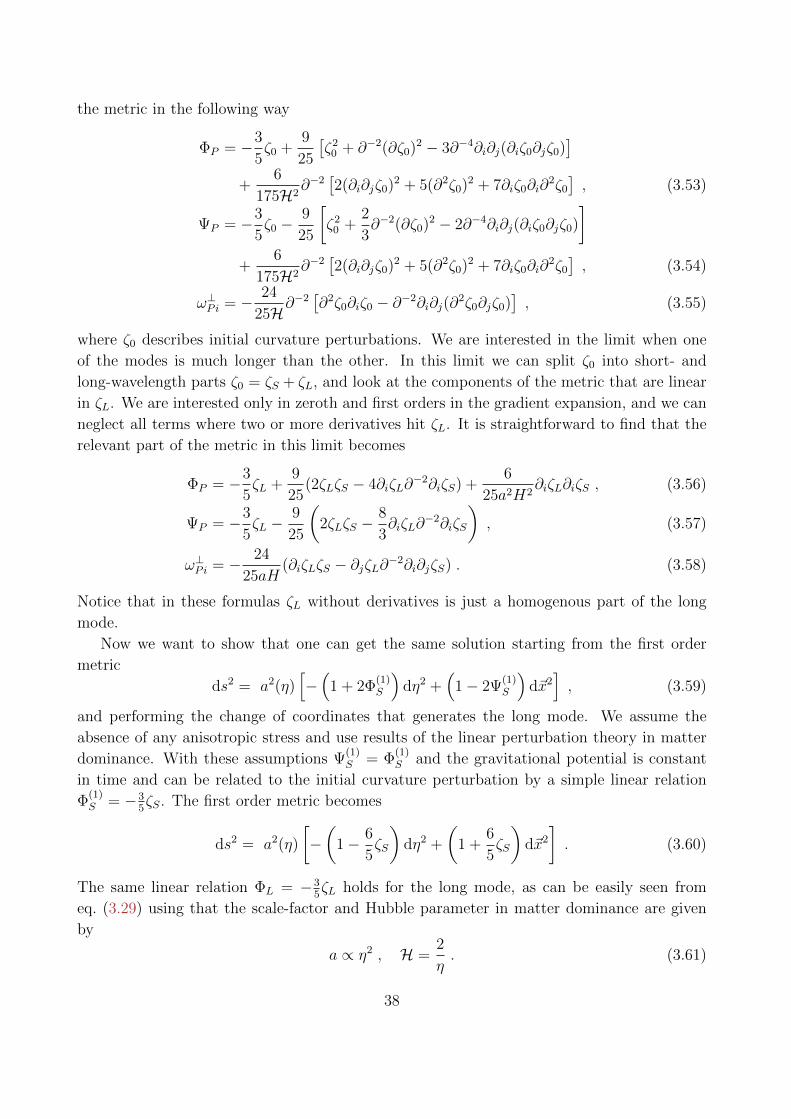
the metric in the following way
ΦP = −3
5ζ0 +
9
25
[ζ2
0 + ∂−2(∂ζ0)2 − 3∂−4∂i∂j(∂iζ0∂jζ0)]
+6
175H2∂−2
[2(∂i∂jζ0)2 + 5(∂2ζ0)2 + 7∂iζ0∂i∂
2ζ0
], (3.53)
ΨP = −3
5ζ0 −
9
25
[ζ2
0 +2
3∂−2(∂ζ0)2 − 2∂−4∂i∂j(∂iζ0∂jζ0)
]+
6
175H2∂−2
[2(∂i∂jζ0)2 + 5(∂2ζ0)2 + 7∂iζ0∂i∂
2ζ0
], (3.54)
ω⊥Pi = − 24
25H∂−2[∂2ζ0∂iζ0 − ∂−2∂i∂j(∂
2ζ0∂jζ0)], (3.55)
where ζ0 describes initial curvature perturbations. We are interested in the limit when one
of the modes is much longer than the other. In this limit we can split ζ0 into short- and
long-wavelength parts ζ0 = ζS + ζL, and look at the components of the metric that are linear
in ζL. We are interested only in zeroth and first orders in the gradient expansion, and we can
neglect all terms where two or more derivatives hit ζL. It is straightforward to find that the
relevant part of the metric in this limit becomes
ΦP = −3
5ζL +
9
25(2ζLζS − 4∂iζL∂
−2∂iζS) +6
25a2H2∂iζL∂iζS , (3.56)
ΨP = −3
5ζL −
9
25
(2ζLζS −
8
3∂iζL∂
−2∂iζS
), (3.57)
ω⊥Pi = − 24
25aH(∂iζLζS − ∂jζL∂−2∂i∂jζS) . (3.58)
Notice that in these formulas ζL without derivatives is just a homogenous part of the long
mode.
Now we want to show that one can get the same solution starting from the first order
metric
ds2 = a2(η)[−(
1 + 2Φ(1)S
)dη2 +
(1− 2Ψ
(1)S
)d~x2], (3.59)
and performing the change of coordinates that generates the long mode. We assume the
absence of any anisotropic stress and use results of the linear perturbation theory in matter
dominance. With these assumptions Ψ(1)S = Φ
(1)S and the gravitational potential is constant
in time and can be related to the initial curvature perturbation by a simple linear relation
Φ(1)S = −3
5ζS. The first order metric becomes
ds2 = a2(η)
[−(
1− 6
5ζS
)dη2 +
(1 +
6
5ζS
)d~x2
]. (3.60)
The same linear relation ΦL = −35ζL holds for the long mode, as can be easily seen from
eq. (3.29) using that the scale-factor and Hubble parameter in matter dominance are given
by
a ∝ η2 , H =2
η. (3.61)
38

In the absence of any anisotropic stress, ΦL = ΨL and eq. (3.28) gives ε = −ηλ/5 and~ξ = −2η~b/5. The coordinate transformation (3.37) and (3.38) under all these assumptions
become
η → η − η
5ζL −
η
5∂iζLx
i − 12
25η ∂iζL∂
−2∂iζS , (3.62)
xi → xi + xiζL + ∂jζLxjxi − 1
2~x2∂iζL −
η2
10∂iζL . (3.63)
Notice that in these expressions ζL and ∂iζL do not depend on space and denote coefficients
of the first two terms in the Taylor expansion of the long mode around the origin.
Let us see how the linear metric transforms. The scale factor changes as
a2(η) → a2(η) (1 + 2Hδη) = a2(η)
(1 +
4
ηδη
), (3.64)
where we have used that 2H = 4/η in matter dominance. The transformation of the short
modes is
ζS → ζS + ∂iζSδxi , (3.65)
while
d~x2 → d~x2(1 + 2ζL + 2∂iζLx
i)− 2
5η∂iζLdxidη , (3.66)
and
dη2 → dη2
(1− 2
5ζL −
2
5∂iζLx
i − 24
25∂iζL∂
−2∂iζS
)− 24
25η ∂jζL
∂j∂i∂2
ζS dxidη . (3.67)
Now we are ready to see how the first order metric transforms. Apart from terms linear in
ζL and ζS, we generate the second order terms O(ζSζL). This is the non-trivial part of the
metric that we are interested in. It can be written in the form
ds2 ⊃ a2(η)
[−(
1 + 2ΦP −6
5∂iζS
(xiζL + ∂jζLx
jxi − 1
2~x2∂iζL
))dη2
+ 2ω⊥Pidxidη +
(1− 2ΨP +
6
5∂iζS
(xiζL + ∂jζLx
jxi − 1
2~x2∂iζL
))d~x2
],
(3.68)
where ΦP and ΨP are exactly the second order solutions in the squeezed limit given by
eq. (3.56).
We showed that the change of coordinates indeed generates the correct second-order so-
lution, with some additional terms in eq. (3.68). These terms are nothing but a dilation and
a special conformal transformation acting on the initial curvature perturbations. Indeed, we
can expect these terms to appear, because the effect of the long mode does not show up only
in the dynamics of the short modes, but also in the possible correlations in the initial con-
ditions. We will come back to this issue later and see that this is the root of the connection
between the consistency relations for inflation and LSS.
39

3.3.2 The Squeezed Limit of δ(2) in a Matter Dominated Unverse
Another way to do this check is to use the density contrast δ calculated at second order
in perturbation theory in a matter dominated universe. Being a second order result, δ(2)~k
is
proportional to a product of two initial conditions Φ~qΦ~k−~q. In the limit when one of these
two modes is much longer than the other q k, δ(2)~k
can be obtained starting from a first
order solution δ(1)~k
and performing the change of coordinates (3.62) and (3.63). Although the
underlying physics is the same as in the previous section, we show this check here because it
shows some technical subtleties that will be relevant later for the derivation of the consistency
relations. The check for a homogeneous long mode was first done in [109], and including
gradients in [67].
The full result for second order δ(2) is given by (see for example [109])
δ(2)~k
= 2
[(k4
14+
3
28(q2
1 + q22)k2 − 5
28(q2
1 − q22)2
)η4
+
(59
14k2 − 125
14(q2
1 + q22)− 9
7
(q21 − q2
2)2
k2
)η2
+
(90 + 36
q21 + q2
2
k2− 54
(q21 − q2
2)2
k4
)]Φ~q1Φ~q2
36. (3.69)
To simplify the notation, here and in the following we assume a summation∫
d3q1 d3q2(2π)3 δ(~k −
~q1 − ~q2) in all products of first order terms in Fourier space. In the limit q1 q2, when one
mode is much longer than the other, we get
δ(2)~k
= 2
[72− 6q2
2η2 +
~q1 · ~q2
q22
(144 + 11η2q2
2 +1
2η4q4
2
)]Φ~q1Φ~q2
36
[1 +O(q2
1/q22)]. (3.70)
We are going to show that this solution is the same as the one that can be obtained starting
from the linear δ(1)
δ(1)~k
= −(12 + k2η2)Φ~k
6, (3.71)
and performing the change of coordinates (3.62) and (3.63).
Notice that δ does not transform linearly under the change of coordinates. Only the
density ρ is a scalar. Therefore, the correct transformation for density contrast is
δ → δ + δη
(ρ′
ρ(1 + δ) + δ′
)+ δxi · ∂iδ . (3.72)
with ρ ∝ η−6 during matter dominance. In order to make the discussion more clear, we split
the check in two parts. First we do the check at order O(q0) (which corresponds to a constant
ΦL) and then we focus on order O(q1) (for which the long mode is proportional to a constant
gradient).
Constant ΦL. In this case we can neglect terms with derivatives ∂iΦL and the change of
coordinates is simply given by
η → η +η
3ΦL , xi → xi − 5
3xiΦL . (3.73)
40
Using eq. (3.72) we find that δ transforms as
δ → δ − 2ΦL − 2ΦLδ +η
3ΦLδ
′ − 5
3ΦLx
i∂iδ . (3.74)
which in Fourier space becomes
δ~k → δ~k − 2Φ~qδ~k +1
3Φ~qηδ
′~k
+5
3Φ~q∂ki(kiδ~k) . (3.75)
We can write δ~k as Tk(η)Φ~k, where Φ describes the first-order (time-independent) potential
in the matter dominated phase, whose value is obviously affected by the evolution during
radiation dominance. Tk(η) describes the linear relation between δ and Φ during MD and it
is given by
Tk(η) ≡ −2− k2η2
6. (3.76)
Plugging this back in the transformation of δ, eq. (3.72), we get
δ~k → δ~k + Φ~qΦ~k
(−2Tk +
1
3ηT ′k +
5
3k∂kTk
)+
5
3Φ~qTk∂ki(kiΦ~k) . (3.77)
The last term describes the effect of a dilation of the initial conditions. We already met these
terms before (see Section 3.3.1), and as we explained they come from the effect of the long
mode on the initial conditions. We will neglect them in what follows, because they do not
contribute to the dynamical evolution that we are trying to capture. With this in mind we
have
δ~k → δ~k + Φ~qΦ~k
(4− 1
3k2η2
). (3.78)
By replacing ~q = ~q1 and ~k = ~q1 + ~q2, this expression reproduces the first two terms in the
eq. (3.70).
Gradient of ΦL. When we add a constant gradient to the coordinate transformation (3.73)
the situation becomes a bit more complicated. Let us look at it term by term by starting
from the time redefinitions eq. (3.63). The last term on the right-hand side gives
δ~k → δ~k +8~q · ~kk2
Φ~q Φ~k , (3.79)
while the second term, i.e. the space-dependent transformation, gives
δ~k → δ~k + 2Φ~q qi∂kiδ~k −1
3Φ~q qiη∂kiδ
′~k. (3.80)
Replacing δ~k = Tk(η)Φ~k, this expression can be rewritten as
δ~k → δ~k +~q · ~kk
Φ~q
(2∂kTk −
1
3η∂kT
′k
)Φ~k + Φ~q
(2Tk −
1
3ηT ′k
)(qj∂kjΦ~k
). (3.81)
41
The last term contains a derivative acting on the initial conditions that we drop for the same
reasons as explained above.
Let us now discuss the spatial redefinitions, given by eq. (3.62). The last term on the
right-hand side gives
δ~k → δ~k −1
6η2~q · ~kΦ~qTkΦ~k . (3.82)
The two remaining terms in the transformation of xi give
δ~k → δ~k −5
6Φ~qqj
[2∂ki∂kj(kiδ~k)− ∂ki∂ki(kiδ~k)
]. (3.83)
After replacing δ~k = Tk(η)Φ~k, this expression can be conveniently rewritten as
δ~k → δ~k −5
6Φ~q
~q · ~kk
(4∂kTk + k∂2
kTk)
Φ~k + 2qjk∂kTk ∂kjΦ~k
+ qjTk[2∂ki∂kj(kiΦ~k)− ∂ki∂ki(kiΦ~k)
].
(3.84)
Similarly to what happened in eq. (3.77), the last two terms of this expression—the ones
proportional to Tk—contain derivatives acting only on the initial conditions and we neglect
them. In the second term one derivative acts on Tk and the other on Φ~k. Adding this term
to the last one on the right-hand side of eq. (3.81) gives
− Φ~q · (qj∂kjΦ~k)
(−2Tk +
1
3ηT ′k +
5
3ki∂kiTk
). (3.85)
Since Φ~k−~q ' Φ~k − (qj∂kjΦ~k), this is just a shift ~k → ~k − ~q in the momentum dependence of
the initial condition in the dilation transformation, eq. (3.77).
Combining all the contributions, i.e. eqs. (3.77), (3.79), (3.81), (3.82) and (3.84), and
dropping derivatives acting on the initial conditions which as already mentioned will be treated
in the next section, we finally obtain
δ~k → δ~k +
(−2Tk +
1
3ηT ′k +
5
3ki∂kiTk
)Φ~qΦ~k−~q
+~q · ~kk2
(8− 4
3k∂kTk −
5
6k2∂2
kTk −1
3ηk∂kT
′k −
1
6η2k2Tk
)Φ~qΦ~k .
(3.86)
We can now plug in the expression for the transfer function, eq. (3.76), and obtain
δ~k → δ~k + 12(12− k2η2)Φ~qΦ~k−~q
36+ 2
~q · ~kk2
(144 + 23η2k2 +
1
2η4k4
)Φ~qΦ~k
36. (3.87)
For ~q = ~q1 and ~k = ~q1 + ~q2, this expression reproduces (after expanding the second term on
the right-hand side) the squeezed limit q1 q2 of the explicit result [109], i.e. eq. (3.70).
42

3.3.3 The Cubic Action for Single-field Inflation
One can do similar checks on the level of the metric in ζ-gauge. Here we are going to focus on
the cubic action for curvature perturbation ζ in standard single-field slow-roll inflation. We
will show that, in the limit in which one of the three modes is much longer than the other
two, this action can be obtained with a coordinate transformation starting from the quadratic
action (up to corrections quadratic in the long-wavelength momentum ~q). The check at zeroth
order in ~q was originally done in [47] and including gradients in [48]. The quadratic and cubic
actions are given by [43] (see Section 2.2)
S(2) =
∫d3xdt εa3
[ζ2 −
(∂ζ
a
)2], (3.88)
S(3) =
∫d3xdt
[aeζ(
1 +ζ
H
) (−2∂2ζ − (∂ζ)2
)+ εa3e3ζ ζ2
(1− ζ
H
)+
+a3e3ζ
(1
2
(∂i∂jψ∂i∂jψ − (∂2ψ)2
) (1− ζ
H
)− 2∂iψ∂iζ∂
2ψ
)], (3.89)
where ψ = − ζa2H
+ χ and ∂2χ = εζ.
We first find the limit of the cubic action when one of the modes is much longer than the
others. To do that, we separate long and short modes by writing ζ = ζL + ζS. Notice that
ζL = O(q2) and whenever a time derivative acts on ζ we can replace it with ζS. Obviously,
the same is true if two spatial derivatives act on ζ. The cubic action then becomes
S(3)q→0 =
∫d3xdt
[aeζ
(1 +
ζSH
)(−2∂2ζS − (∂ζ)2
)+ εa3e3ζ ζS
2(
1− ζSH
)+
+a3e3ζ
(1
2
(∂i∂jψS∂i∂jψS − (∂2ψS)2
) (1− ζS
H
)− 2∂iψ∂iζ∂
2ψS
)], (3.90)
We are interested in terms linear in ζL and quadratic in ζS. We can expand the action
and try to simplify it using integration by parts. For example, the second term in S(3)q→0 gives
εa3e3ζ ζS2(
1− ζSH
)→ 3εa3ζLζ
2S . (3.91)
The other terms demand a bit more work. The first term in S(3)q→0 gives
aeζ(
1 +ζSH
) (−2∂2ζS − (∂ζ)2
)→ aeζL+ζS
(1 +
ζSH
) (−2∂2ζS − (∂ζS)2 − 2∂iζL∂iζS
)→ aζL(∂ζS)2 − 2aζL
ζSH∂2ζS − 2a∂iζL
ζSH∂iζS , (3.92)
43

where we have expanded the exponent eζL+ζS = 1 + ζL + ζS + ζLζS + · · · and have done
one integration by parts: aζLζS∂2ζS → −aζL(∂ζS)− a∂iζLζS∂iζS. Now we can transform the
second term in the previous expression
−2aζLζSH∂2ζS → 2a∂iζL
ζSH∂iζS +
a
HζL
d
dt[(∂ζS)2]
→ 2a∂iζLζSH∂iζS − aζL(∂ζS)2 − aεζL(∂ζS)2 , (3.93)
such that the first term in S(3)q→0 finally simplifies to
aeζ(
1 +ζSH
) (−2∂2ζS − (∂ζ)2
)→ −aεζL(∂ζS)2. (3.94)
Now we can focus on the last term in S(3)q→0. After expanding the exponent, the relevant part
is given by
3
2a3ζL
(∂i∂jψS∂i∂jψS − (∂2ψS)2
)− 2a3∂iζL∂iψS∂
2ψS − 2a3∂iψL∂iζS∂2ψS . (3.95)
The first contribution can be rewritten as
3
2a3ζL∂i
(∂jψS∂i∂jψS − ∂iψS∂2ψS
)=
3
4a3ζL∂
2(∂ψS)2 − 3
2a3ζL∂i
(∂iψS∂
2ψS)
→ 3
4a3(∂2ζL)(∂ψS)2 +
3
2a3∂iζL∂iψS∂
2ψS . (3.96)
The first term on the left hand side has two spatial derivatives on ζL and it can be neglected
while the second one has the same form as the second term in (3.95). If we rewrite it as
∂iζL∂iψS∂2ψS = ∂iζL∂j(∂iψS∂jψS)− 1
2∂iζL∂i(∂ψS)2 , (3.97)
we can see that, after integration by parts, it is proportional to ∂2ζL too, and can be safely
neglected. To summarise, only the last term in (3.95) gives a non-vanishing contribution to
the cubic action in the limit we consider. It can be further simplified noticing that one is
forced to replace ∂2ψS with ∂2χS = εζS, because otherwise a term with two spatial derivatives
on ζL is generated again. At leading order in slow-roll ∂iψL = − 1a2H
∂iζL, and finally we get
− 2a3∂iψL∂iζS∂2ψS →
2aε
H∂iζLζS∂iζS . (3.98)
Summing up all relevant contributions in the cubic action linear in ζL and quadratic in ζS we
get
δS(3)q→0 =
∫d3xdt
(3εa3ζLζ
2S − aεζL(∂ζS)2 +
2aε
HζS∂iζS∂iζL
). (3.99)
On the other hand, we can start from the quadratic action for the short modes and perform
a change of coordinates
xi → xi = xi − bix2 + 2xi(b · x) + δxi(t) (3.100)
44
with
bi = −1
2∂iζL
d
dtδxi(t) = − 2bi
a2H+O(ε) . (3.101)
What we expect to find is exactly the cubic action (3.99) with one long and two short modes.
Indeed, starting from the action (3.88) and performing the change of coordinates we get
δS(2) =
∫d3xdt
[−6a3ε(~b · ~x)ζ2 + 2aε(~b · ~x)(∂ζ)2 − 4aε
ζ
Hbi∂iζ
]. (3.102)
This indeed coincides with the cubic action in the squeezed limit once we use bi = −12∂iζL.
Notice that in this check we did an expansion in ζL. However, for the homogeneous ζLthe check can be done exactly, without assuming that ζL is small. To see this, notice that the
long mode appears in the action only in combination aeζL. Therefore, removing the long mode
is equivalent to a finite resealing of the scale-factor [47]. The same does not hold for a large
homogeneous gradient and, as we are going to see later, this has important consequences for
studying multiple soft limits of the inflationary correlation functions.
A similar check can be done for a long tensor mode and two short scalar modes too. The
cubic action in the single field slow-roll inflation in this case is given by
S =
∫d4x
1
2
φ2
H2aγij∂iζ∂jζ . (3.103)
From the form of the action it is immediately clear that the effect of γ is equivalent, including
first gradient corrections, to the change of spatial coordinates discussed above (see eq. (3.49)).
A similar analysis does not work for the vertices ζLγγ and γLγγ when gradient corrections
are included. As we already pointed out (see Section 3.2.2), this is related to the fact that in
the presence of short tensor modes a naive change of coordinates does not induce a proper
long mode and one has to be more careful (see [50]). We will come back to this issue when
we discuss the consistency relations for single-field inflation involving short tensor modes.
45

Chapter 4
Inflationary Consistency Relations
In the previous Chapter we showed that the long-wavelength mode can be locally traded for
a change of coordinates. In this Chapter we are going to use this as a starting point to derive
the consistency relations for single-field inflation. These relations connect the squeezed limit
of an (n+ 1)-point function of curvature perturbations with a variation of the corresponding
n-point function and have the following form
〈ζ~qζ~k1. . . ζ~kn〉
′q→0 =− P (q)
[∑a
Da +O(q/k)2
]〈ζ~k1
. . . ζ~kn〉′ , (4.1)
where Da is some differential operator with derivatives acting on ~ka which is linear in ~q.
Given that the construction of the adiabatic modes is quite general, the consistency rela-
tions will be a very general result too. As we will show in the following sections they hold in
any single-field model of inflation, independently on the details of inflationary potential and
kind of interactions of the inflaton field. We will see that this is a very powerful statement that
allows us to make model-independent observational tests that can rule out any single-field
model of inflation.
Although eq. (4.1) involving soft scalars is best known, one can derive similar consistency
relations for long tensor modes too. Furthermore, it is possible to use these results to in-
vestigate other kinematical regimes where there is a big separation in scales. We will focus
on two examples, one where the sum of some of the external momenta goes to zero and the
other where several external modes are soft. We are also going to discuss in what sense one
can extend some of the arguments that go into the derivation of the consistency relations to
capture also O(q2) corrections in eq. (4.1). Towards the end of this Chapter, we will comment
on the connection of the consistency relations and Ward identities for spontaneously broken
space-time symmetries.
4.1 Consistency Relations for Scalars
In this Section we will focus on the squeezed limit of correlation functions involving only scalar
modes ζ. We will derive Maldacena’s consistency relation [43] and its generalisation when
46

gradients of the long mode are included—conformal consistency relation [48]. After giving
some comments on the assumptions behind the derivation and importance of the consistency
relations, we will give several non-trivial checks using explicit expressions for correlation
functions calculated in several single-field models.
Let us begin with a physical argument that is behind the consistency relations [43, 45].
Given that we are interested in calculating the squeezed limit of an (n + 1)-point function,
the configuration that we are considering in real space is the one where one mode is much
longer than other short modes. It is obvious that during inflation the long mode goes outside
the horizon first and by the time the short modes cross the horizon (which is the moment
when the in-in integral picks up the most of the contribution), it can be considered as a
classical background for the short modes. As we saw in the previous Chapter this background
is equivalent to a simple change of coordinates, including first order in gradients. Therefore,
performing a proper change of coordinates, we can go to a frame in which the long mode
is removed. Essentially, this is what allows us to write down the consistency relations: the
change of coordinates relates two solutions, with and without the long mode and the same
short modes, and consequently the (n+ 1)-point and n-point correlation functions.
Let us make this line of reasoning a bit more quantitative. The starting point is a statement
in real space that, for the correlation functions of short modes, the presence of ζL can be
identified with a change of coordinates. In other words
〈ζ(x1) · · · ζ(xn)|ζL〉 = 〈ζ(x1) · · · ζ(xn)〉 , (4.2)
where the change of coordinates is such that going from x to x corresponds to generating ζL.
Our aim now is to rewrite this equality in terms of standard correlation functions. In order
to do that, we should multiply both sides with ζL and average over it⟨ζL(x)〈ζ(x1) · · · ζ(xn)|ζL〉
⟩=⟨ζL(x)〈ζ(x1) · · · ζ(xn)〉
⟩. (4.3)
Notice that the left hand side is just an (n + 1)-point function involving ζL and n short
modes. The right hand side is a bit more complicated, because x contains ζL and in general
one cannot find the average over ζL easily. However, we can expand the n-point function in
δx and take the average after that1. The first two terms in the expansion are
〈ζ(x1) · · · ζ(xn)〉 = 〈ζ(x1) · · · ζ(xn)〉+n∑a=1
δxai · ∂ai〈ζ(x1) · · · ζ(xn)〉+ · · · . (4.4)
If we plug this expression into eq. (4.3) the first term is proportional to 〈ζL〉 and averages
to zero. Therefore, on the right hand side, the only relevant contribution comes from the
variation of the n-point function
δ〈ζ(x1) · · · ζ(xn)〉 =n∑a=1
δxai · ∂ai〈ζ(x1) · · · ζ(xn)〉 . (4.5)
1We will come back later to the case in which we keep the coordinate transformation finite when we talk
about multiple soft limits.
47

Finally, what we can write down in real space is the following equality
〈ζL(x)ζ(x1) · · · ζ(xn)〉 =⟨ζL(x) ·
n∑a=1
δxai · ∂ai〈ζ(x1) · · · ζ(xn)〉⟩. (4.6)
This is the consistency relation written in real space. On the left hand side we have the
(n + 1)-point function. On the right hand side, the average 〈ζL · δx〉 gives the two point
function of the long mode, multiplying a variation of the n-point function. To bring this
result to the familiar form, one only has to rewrite this equation in momentum space.
Of course, in order to do that, one has to specify the change of coordinates δx. In the
following two sections we are going to split the discussion. First, we are going to consider only
the homogeneous part of the long mode that corresponds to a dilation of spatial coordinates.
After that we will turn to the case where gradients are included as well and the change of
coordinates contains both dilations and special conformal transformations.
Before moving on, let us introduce some notation that we are going to use here and in the
following chapters. We define
d~k1
(2π)3· · · d~kn
(2π)3≡ dKn , 〈ζ~k1
· · · ζ~kn〉 =M · δ(~P ) , ~P = ~k1 + · · ·+ ~kn , (4.7)
and M contains all momentum dependence of the correlation function other than the delta
function of momentum conservation.
4.1.1 Maldacena’s Consistency Relation
At zeroth order in gradients, the result of the procedure described above is Maldacena’s
famous consistency relation. It was first proven to hold in standard single-field slow-roll
inflation [43] and later it was shown that it is valid in all inflationary models with a single
dynamical degree of freedom, independently on the slow-roll approximation and the form of
the interactions [45, 46].
Let us follow the main steps in the derivation. The long mode at leading order in deriva-
tives, as we saw in Section 3.2.1, is equivalent just to a simple time-independent rescaling of
spatial coordinates
xi → xi + ζL(~x+)xi . (4.8)
For the homogeneous long mode the point ~x+ is arbitrary, but physically it should be in the
neighbourhood of the points ~x1, . . . , ~xn. For concreteness we will make the following choice
~x+ = (~x1 + · · ·+ ~xn)/n.
We can start from eq. (4.5) and rewrite it in momentum space. Using δ~x = ζL(~x+)~x, the
variation of an n-point function is
δ〈ζ(x1) · · · ζ(xn)〉 =
∫d~q+
(2π)3dKn ζ~q+
∑a
Mδ(~P )kai∂kaiei~q+·~x++i~kb·~xb
= −∫
d~q+
(2π)3dKn ζ~q+
∑a
(3Mδ(~P ) + kai∂kaiMδ(~P ) + kaiM∂kaiδ(
~P ))ei~q+·~x++i~kb·~xb , (4.9)
48
where we did one integration by parts to go to the second line. Notice that in the exponent
we implicitly assume the summation over b which runs from 1 to n. The term that needs
additional simplification is the one where derivatives act on the delta function. First, notice
that we can write ∂kaiδ(~P ) = ∂Piδ(
~P ). After this replacement it is easy to do the sum, and
the last term becomes M~P · ~∂P δ(~P ). We still have derivatives acting on the delta function
and we have to do integration by parts again. What we gained in rewriting the last term in
this form is that whenever the derivative hits anything else than ~P , the result is proportional
to the integral of ~Pδ(~P ) and therefore is zero. Having this in mind, we can finally write
δ〈ζ(x1) · · · ζ(xn)〉 = −∫
d~q+
(2π)3dKn ζ~q+
[(3(n− 1) +
∑a
kai∂kai
)M]δ(~P )ei~q+·~x++i~kb·~xb ,
(4.10)
where now derivatives act only on M.
To complete the derivation we should only multiply this expression by the long mode
ζ(x) and average over it. As we already said, on the left hand side we are going to get the
(n+ 1)-point function while on the right hand side we get the two-point function of the long
mode. After integrating one of the momenta ~q+, we are left with
〈ζ(x)ζ(x1) · · · ζ(xn)〉 = −∫
d~q
(2π)3dKn P (q)
(3(n− 1) +
∑a
kai∂kai
)Mδ(~P )ei~q·~x+i~kb·~xb .
(4.11)
On the other hand, the Fourier transform of the (n+ 1)-point correlation function is given by
〈ζ(x)ζ(x1) · · · ζ(xn)〉 =
∫d~q
(2π)3dKn〈ζ~qζ~k1
· · · ζ~kn〉′(2π)3δ(~q + ~P )ei~q·~x+i~kb·~xb (4.12)
We can directly compare these two expressions to get Maldacena’s consistency relation [43]
〈ζ~qζ~k1· · · ζ~kn〉
′~q→0 = −P (q)
(3(n− 1) +
∑a
kai∂kai +O(q/k)
)〈ζ~k1· · · ζ~kn〉
′ . (4.13)
Notice that in the two integrals we have delta functions of momentum conservation with
different arguments. At zeroth order in ~q this difference is irrelevant. Of course, when we
include first order in gradients of the long mode, this subtlety will become important. We
will come back to this issue in the following Section when we derive the conformal consistency
relation for single-field inflation.
4.1.2 Conformal Consistency Relations
Maldacena’s consistency relation describes the squeezed limit of an (n+ 1)-point function at
leading order in gradients of the long mode. However, as we saw in Chapter 3.2.1, the long
mode is equivalent to a change of coordinates including gradients. This implies that we can
49

use the same arguments as in previous sections to derive a consistency relation that captures
O(q) corrections in the squeezed limit of an (n+ 1)-point function. Given that at this order
the long mode is equivalent to a special conformal transformation of the spatial coordinates,
the squeezed limit will be related to a conformal variation of the n-point function. For this
reason we call these relations conformal consistency relations [48].
Before we move to the derivation, let us stress here one important difference compared
to Maldacena’s consistency relation. While the inflationary correlation functions are almost
scale invariant, they are not invariant under special conformal transformations. Therefore,
while in the limit of exact scale invariance the right hand side of Maldacena’s consistency
relation gives just zero, the conformal consistency relation will have a nontrivial contribution.
One easy way to understand where this difference is coming from is to consider the decou-
pling limit. In this limit we are interested in correlation functions of small fluctuations around
the inflaton background φ(t). As we already explained in the Introduction, the time-dependent
inflaton background breaks de Sitter isometries spontaneously. Two of these isometries, in
the late time limit η → 0, act as dilation and special conformal transformation of spatial
coordinates, and one would expect that the correlation functions are not invariant under any
of these two transformations. However, the approximate shift symmetry of the inflaton field
φ → φ + C is what makes the correlation functions almost scale-invariant. On the other
hand, the isometries corresponding to the spatial conformal transformation for η → 0 remain
broken. We will come back to this discussion in the following sections.
The derivation of the conformal consistency relations is essentially the same as for Mal-
dacena’s consistency relation. Again, we can start from eq. (4.5). The only difference now
is that we have to use a more complicated change of coordinates that induces not only the
homogeneous part of the long mode but also the homogeneous gradient. We already saw that
this change of coordinates is
xi → xi + ζLxi + (∇ζL · ~x)xi − 1
2~x2∇iζL + δxi(t) , (4.14)
where the time-dependent translation is such that N iL(t) = −δxi(t). The explicit form of
this term is irrelevant, since all correlation functions are translationally invariant and in what
follows we will drop it. Notice that in this expression ζL is just a homogenous part of the
long mode while ∇ζL is a homogeneous gradient: ζL(x) = ζL +∇ζL · ~x. We also assume that
ζL and ∇ζL are evaluated at ~x+. As we will see, the choice of this point is irrelevant, but for
concreteness we will use the midpoint ~x+ ≡ (~x1 + . . .+ ~xn)/n.
Using the explicit form of the change of coordinates, the variation of the n-point function
in momentum space is given by
δ〈ζ(x1) · · · ζ(xn)〉 =
∫d~q+
(2π)3dKn ζ~q+
∑a
Mδ(~P )
×(kai∂kai + q+jkai∂kai∂kaj −
1
2q+ikai∂kaj∂kaj
)ei~q+·~x++i~kb·~xb . (4.15)
50

The only thing that remains to be done is to do some integrations by parts and rewrite this
expression such that all derivatives act on M and the delta function factors out. The first
term in brackets comes from the rescaling of coordinates and we already saw how to deal with
it. It will contribute to the final result as
δ〈ζ(x1) · · · ζ(xn)〉 ⊃ −∫
d~q+
(2π)3dKn ζ~q+
(3(n− 1) +
∑a
kai∂kai
)Mδ(~P )ei~q+·~x++i~kb·~xb .
(4.16)
The nontrivial exercise is to rewrite the other two terms in eq. (4.15). If we do two integrations
by parts we get
δ〈ζ(x1) · · · ζ(xn)〉 ⊃∫
d~q+
(2π)3dKn ζ~q+
×∑a
(q+j∂kai∂kaj(kaiMδ(~P ))− 1
2q+i∂kaj∂kaj(kaiMδ(~P ))
)ei~q+·~x++i~kb·~xb . (4.17)
Let us look at the integrand in more detail. If we expand the derivatives we get
∂kai∂kaj(kaiMδ(~P )) = 4∂kajM · δ(~P ) + kai∂kai∂kajM · δ(~P )
+ 4M∂kajδ(~P ) + kai∂kajM∂kaiδ(
~P ) + kai∂kaiM∂kajδ(~P )
+ kaiM∂kai∂kajδ(~P ) . (4.18)
Similarly, the other term is
−1
2∂kaj∂kaj(kaiMδ(~P )) = −∂kaiM · δ(~P )− 1
2kai∂kaj∂kajM · δ(~P )
−M∂kaiδ(~P )− kai∂kajM∂kajδ(
~P )
− 1
2kaiM∂kaj∂kajδ(
~P ) . (4.19)
All terms in the first lines of these two expressions are proportional to δ(~P ) and we do not
have to do any additional work to bring them to the right form. They will contribute to the
final result as
δ〈ζ(x1) · · · ζ(xn)〉 ⊃∫
d~q+
(2π)3dKn ζ~q+
×∑a
1
2q+i
(6∂kai + 2kaj∂kaj∂kai − kai∂kaj∂kaj
)M · δ(~P )ei~q+·~x++i~kb·~xb . (4.20)
Now we can focus on terms with one derivative on δ(~P ). They are in the second lines of
equations (4.18) and (4.19). If we combine them we get two kind of contributions. One will
be of the form ∑a
qi∂Pjδ(~P ) ·
(kaj∂kai − kai∂kaj
)M . (4.21)
51

This is just a rotation operator acting onM, and since the correlation functions are rotation-
ally invariant the action of this operator is zero. The remaing contribution is just
δ〈ζ(x1) · · · ζ(xn)〉 ⊃∫
d~q+
(2π)3dKn ζ~q+
×(
3n+∑a
kai∂kai
)M · q+i∂Piδ(
~P )ei~q+·~x++i~kb·~xb . (4.22)
Notice that this is almost the form of the dilation operator. The missing part comes from the
terms with two derivatives on the delta function. After we do two integrations by parts, they
are schematically of the form
qjδ(~P ) · ∂Pi∂Pj(Pi ·X) = 4qjδ(~P ) · ∂PjX + qjδ(~P )Pi · ∂Pi∂PjX . (4.23)
and
− 1
2qjδ(~P ) · ∂Pi∂Pi(Pj ·X) = −qjδ(~P ) · ∂PjX −
1
2qjδ(~P )Pj · ∂Pi∂PiX . (4.24)
Terms proportional to Piδ(~P ) under the integral give zero. Therefore, the only remaining
contribution to the variation of the n-point function, after another integration by parts, is
just given by
δ〈ζ(x1) · · · ζ(xn)〉 ⊃∫
d~q+
(2π)3dKn ζ~q+q+i (−3)M · ∂Piδ(~P )ei~q+·~x++i~kb·~xb . (4.25)
Combining equations (4.16), (4.22) and (4.25), we get at the end
δ〈ζ(x1) · · · ζ(xn)〉 ⊃ −∫
d~q+
(2π)3dKn ζ~q+
×(
3(n− 1) +∑a
kai∂kai
)M · (1− q+i∂Pi)δ(
~P )ei~q+·~x++i~kb·~xb . (4.26)
Notice that all these complicated contributions at the end just give the dilation operator
multiplying (1− q+i∂Pi)δ(~P ). It was crucial to bring the variation of the n-point function in
this form, because we can write
(1− q+i∂Pi)δ(~P ) = δ(~P − ~q+) (4.27)
up to corrections of order O(q2+). After we average over the long mode ζ~q and integrate in ~q+,
this delta function will become δ(~P + ~q), which is exactly what we have on the left hand side
when we write the Fourier transform of the (n+ 1)-point function. This kind of manipulation
is not necessary for the expression (4.20) because it is already first order in ~q+.
After this long and rather technical procedure, summing up (4.20) and (4.26) and averaging
over the long mode ζ~q, we get the final result: the consistency relation valid up to corrections
of order O(q2/k2)
〈ζ~qζ~k1. . . ζ~kn〉
′q→0 =− P (q)
[3(n− 1) +
∑a
~ka · ~∂ka +1
2qiδ
(n)
Ki +O(q/k)2
]〈ζ~k1
. . . ζ~kn〉′ ,
(4.28)
52

where the operator δ(n)
Ki is the operator of special conformal transformation acting in momen-
tum space
qiδ(n)
Ki ≡n∑a=1
[6~q · ~∂ka − ~q · ~ka~∂2
ka + 2~ka · ~∂ka(~q · ~∂ka)]. (4.29)
In the case where the n-point function depends only on the magnitudes of the momenta |~ka|,this operator simply becomes [40]
n∑a=1
~q · ~ka[
4
ka
∂
∂ka+
∂2
∂k2a
]. (4.30)
Notice that the procedure above implies that the same delta function of momentum con-
servation is removed from the correlation functions on both sides. For conformal consistency
relation this is not relevant because the variation of the n-point function is explicitly propor-
tional to q. However, this statement is not trivial for the scale variation. What we actually
see is that the n-point function has to be evaluated for a configuration of momenta ~k1 . . . , ~knthat do not form a closed polygon, but ~k1 + · · ·+~kn = −~q. Operationally, this means that in
order to properly calculate O(q) terms in the squeezed limit, on has to apply the first operator
in eq. (4.28) on the n-point function and after that expand it in q having in mind that∑~ka
is not zero. We will check this explicitly in some examples later.
The procedure we described might seem a bit confusing and ambiguous. The correlation
functions that we calculate using the in-in formalism are always such that the sum of mo-
menta is equal to zero. Therefore, it seems that there are many possible extensions to go to
configurations where momenta do not form a closed polygon. In other words, we can always
add to the n-point function a term of the form Madd = ~P · ~F (~k), where F is an arbitrary
function. On the other hand, it so not obvious that this does not change the right hand side
of the consistency relation.
In the short calculation that follows we are going to show that indeed this is exactly what
happens and the consistency relation is unambiguous. To do that we will calculate the action
of the operator (3(n− 1) +
∑a
kai∂kai +1
2qiδ
(n)
Ki
)(4.31)
on the additional amplitude Madd. It is straightforward to find that, keeping only linear
terms in ~q, we get that the action of the operator is given by
3(n− 1)PiFi +∑a
kaj(Fi + Pi∂kajFi) + 3∑a
qiFi −∑a
qjkaj∂kaiFi
+∑a
qjkai∂kaiFj +∑a
qjkai∂kajFi . (4.32)
After some trivial algebra, these terms can be rearranged in the following way
(Pi + qi)
[3(n− 1) +
∑a
kal∂kal
]Fi + 2qiFi + qj
∑a
(kai∂kaj − kaj∂kai)Fi . (4.33)
53

The first term is zero because ~P + ~q = 0. The other two terms cancel after we rewrite the
function F in the following way
Fi =∑a
kaiAa , (4.34)
where Aa are scalar functions of the momenta and they are rotationally invariant. Indeed,
this can be always done without loss of generality.
4.1.3 Comments
Before we move to checks of the consistency relations, let us pause for a bit and comment on
some of their properties. First of all, we derived the consistency relations without specifying
the details of the underlying physics driving inflation and creating the perturbations. In
particular, although the consistency relations involve correlation functions, we did not have
to specify any interactions. The only assumption we made is that the long mode always
locally reduces to a diffeomorphism. This is always true in any single-field model of inflation
if the inflaton is on the attractor2. Indeed, if we have only one dynamical degree of freedom
during inflation, then all parts of the universe follow the same classical history and quantum
fluctuations of the inflaton are locally equivalent to a small shift of this classical history in
time. As a consequence, different regions of the universe expand by different amounts, but
they all have the same history. Obviously, the perturbations created in this way are adiabatic.
Under these assumptions, once the long mode crosses the horizon, it becomes frozen and
remains constant. For short modes its effect is not physical because it describes only a small
perturbation in the expansion of the universe that can be removed just by a rescaling of
coordinates. This is exactly what we used in the previous section to derive the consistency
relations. To summarise, in any single-field model of inflation (assuming that the inflaton is on
the dynamical attractor and choosing the Bunch-Davies vacuum), we expect the consistency
relations to hold, independently on the details of interactions, the form of the kinetic term,
slow-roll assumptions or any other details of the theory [45].
One immediate consequence of this statement is that in single-field models we expect small
local non-Gaussianities. Indeed, one can check that the action of conformal operator on the
two-point function vanish at order O(q). On the right hand side of the consistency relation
remains only the dilation operator. Given the approximate scale invariance of the two-point
function, in the squeezed limit of the three-point function we are left with
〈ζ~qζ~k1ζ~k2〉′~q→0 = −
[(ns − 1) +O(q2/k2)
]P (q)P (k) . (4.35)
From this equation we can immediately read that in any single-field model, the amplitude of
local non-Gaussianities f loc.NL is proportional to the tilt of the power spectrum. Of course, this
makes the local non-Gaussianities unobservable in the near future. However, the main point
of this result is that if one observes f loc.NL 1, this would in one shot rule out all single-field
2Notice that here we are assuming standard initial conditions—Bunch-Davies vacuum. We will comment
on this assumption later.
54

models [45]. Therefore, phenomenologically it is much more interesting to look for violations
of the consistency relations, than to try to check if they hold. The current constraints on
non-Gaussianities from Planck are compatible with single-field models. Indeed, the limit is
f loc.NL = 2.7± 5.8 [13].
Notice that eq. (4.35) is written in ζ-gauge and the reader might be worried that going to
observables in the CMB some of the conclusions can change. Although the long mode is always
locally equivalent to an unobservable change of coordinates, the coordinate transformation
can vary from one part of the sky to the other and this can induce some contribution to
the three-point function of temperature fluctuations. Indeed, the squeezed limit of the CMB
bispectrum can be calculated analytically, and the corresponding f loc.NL is given by [64]
f loc.NL = −1
6(1 + 6 cos 2θ)
(1− 1
2
d ln(l2SClS)
d ln lS
), (4.36)
where θ is the relative angle between the long and short modes and Cl the standard temper-
ature angular power spectrum. From this expression we see that in single-field models local
non-Gaussianities are always small, at most f loc.NL ∼ O(1).
On a more theoretical side, being a non-perturbative and a model-independent result, the
consistency relations are a powerful tool and have many applications in the study of single-
field inflationary models. For example, using the consistency relations one can explore the
infrared divergences in calculations of the correlation functions involving loops [92]. They are
also an important ingredient in the proof that ζ is conserved outside the horizon, to all orders
in perturbation theory [91, 92, 93, 94, 95].
Before moving to some more technical comments, let us briefly come back to the assump-
tions that enter the derivation of the consistency relation and see what happens if some of
them are violated. One obvious choice is multi-field inflation. Although in models with
more that one dynamical degree of freedom it might happen that accidentally the local non-
Gaussianities are small too, this is not a generic case. Indeed, multifield models typically
predict large f loc.NL . Some examples include the curvaton mechanism [37, 38] and inhomoge-
neous reheating [110] (for a review see [111]). Even in single-field models, if the inflaton is not
on the attractor, large local non-Gaussianities can be still generated. This kind of violations
of the consistency relations were recently studied in [112]. The same holds if we change the
initial state. In a non-Bunch-Davies vacuum, explicit calculations show that the three-point
function in the squeezed limit can be large [113]. For some recent discussion on this subject
see [114, 115]. Let us at the end point out another interesting example of a single-field infla-
tionary model in which the consistency relation is (in principle) violated—Khronon inflation
[34]. The details of the model are briefly summarised in Appendix A. Let us here just point
out that, due to a peculiar 1/a(t) decay of the decaying modes in Khronon inflation, it is
possible to violate the consistency relations even though all other conditions are satisfied.
Unfortunately, this violation turns out to be very small and suppressed by the small breaking
of the time reparametrization symmetry.
Let us finally come back to eq. (4.28) and comment on some of the consequences for corre-
lation functions and interactions in the Lagrangian. As we already pointed out, Maldacena’s
55

consistency relation is somewhat trivial due to the scale invariance. On the other side, the
conformal consistency relation carries more information, but only for higher order correlation
functions. For example, the conformal variation of the two-point function vanishes (up to
terms which are singular in Fourier space, see [40]). This is obvious from the fact that the
two-point function does not specify any direction with which the vector ~b can be contracted.
This implies that the conformal consistency relation just implies that the three-point function
is suppressed, compared with a local shape, by (at least) O(q/k)2 [47].
Much less trivial is the implication of eq. (4.28) for the squeezed limit of the four-point
function, as we are now going to discuss. First of all, at the level of the Lagrangian, it is
well known that operators with a different number of fields are related due to the non-linear
realization of the Lorentz symmetry [25]. The conformal consistency relations contain the
same information at the level of observable correlation functions. For example, for cs = 1, the
operator (g00+1)3 in the language of the effective field theory of inflation [25], contributes both
to the three-point function and to the four-point function. This is encoded in the conformal
consistency relation, as the conformal variation of the three-point function must be matched
by a corresponding (squeezed limit of the) four-point function.
Similarly, if an operator only contributes to the four-point function and not to the three-
point function, then this four-point function must have a suppressed squeezed limit, i.e. the
coefficient of the q−2 divergence must vanish. This is indeed what happens for the operator
(g00 + 1)4. In [116] it was shown that it is technically natural to make this operator large and
the four-point function arbitrarily large compared to the three-point function: in any case
this happens for any n-point function, its q−2 divergence must vanish.
Finally, the conformal consistency relation eq. (4.28) states that the q−2 divergence of the
four-point function is always small, of order P1/2ζ times the three-point function. This is not
at all obvious at the level of the action. Indeed, the operator which reduces the speed of
sound gives a four-point function of order P1/2ζ c−2
s compared with the three-point function.
Moreover, this operator is of the form (∇π)4 so that it naively gives rise to a q−2 squeezed limit.
It turns out that, in going to the Hamiltonian, the term (∇π)4 gets a c2s suppression while the
leading source of the four-point function (∝ c−4s ) is given by the exchange diagrams which,
as discussed above, do not contribute to the q−2 divergence. The same kind of cancellation
occurs for the operator λπ2(∇π)2 which, in the small cs limit, would naively give a four-point
function which is too large in the squeezed limit to satisfy eq. (4.28). Again, this term is
cancelled in going to the Hamiltonian and gets suppressed by c2s, while the leading four-point
function is given by the exchange diagrams. In the following section we will explicitly check
some of these results.
4.1.4 Checks
Most of the correlation functions for different inflationary models are calculated in the limit
of the exact scale-invariance. For this reason, most of the checks of Maldacena’s consistency
relation that we can do boil down to explicitly proving that at leading order the correlation
56

functions vanish in the limit ~q → 0. If deviations from the perfect scale-invariance are
included in the calculation, then the checks become more nontrivial and one gets nonzero
result on both sides of the consistency relation. For example, one can calculate the three-
point function in models with reduced speed of sound including slow-roll corrections. Then,
taking the squeezed limit, after a long calculation, one indeed recovers that the right hand
side is simply proportional to the tilt of the power spectrum as expected (for the details see
[117]).
〈ζ~qζ~k1ζ~k2〉′~q→0 = −(ns − 1)P (q)P (k) . (4.37)
On the other hand, the conformal consistency relation gives a non-trivial check even in the
limit of exact scale invariance. Unfortunately, as we pointed out, the action of the conformal
operator on the two-point function is always zero. This means that the checks have to include
higher order correlation functions that are more difficult to calculate. We are going to show
a couple of examples involving three-point and four-point functions in different classes of
single-field models.
Resonant non-Gaussianities. Let us first focus on example of models in which scale-
invariance is broken and we can check that eq. (4.13) holds. We are going to consider models
with a periodic modulation of the inflaton potential that have recently attracted some at-
tention, as motivated by explicit string constructions of Monodromy Inflation [118]. These
models represent an interesting example in which the n-point functions deviate sizeably from
scale-invariance and in which many n-point functions can be analytically calculated at leading
order in the parameter describing the potential modulation [119, 120].
The (n+ 1)-point function reads (see Appendix A for more details)
〈ζ~qζ~k1. . . ζ~kn〉 = (2π)3δ(~q + ~k1 + . . .+ ~kn)
(−Hφ
)n+1H2n−2
2q3∏n
i=1 2k3i
In+1 , (4.38)
where In+1 is given by the following in-in integral:
In+1 = −2 Im
∫ 0
−∞−iε
dη
η4V (n+1)(φ(η))(1− iqη)(1− ik1η) . . . (1− iknη)eiktη . (4.39)
Here kt = q +∑
i ki and V (n+1) is the (n + 1)th derivative of the potential, evaluated on
the unperturbed history φ(η). Now we can calculate the squeezed limit of this (n + 1)-point
function and check that it satisfies Maldacena’s consistency relation. In the squeezed limit
q → 0, the expression above gives
〈ζ~qζ~k1. . . ζ~kn〉
′q→0 = −
(−Hφ
)H2
2q3
(−Hφ
)nH2n−4∏ni=1 2k3
i
2 Im
∫ 0
−∞
dη
η4V (n+1)
n∏i=1
(1− ikiη)eikiη .
(4.40)
The trick that we are going to use is to convert the (n+ 1)th derivative of the potential using
d
dφV (n)(φ(η)) = −H
φ
[ηd
dηV (n)(φ(η))
](4.41)
57
and integrate by parts the derivative with respect to η. Given that in the expressions for the
wavefunctions under the integral conformal time always appears in the combination kiη, this
derivative can be traded for derivatives with respect to ki to give
−(H
φ
)2H2
2q3
[3(n− 1) +
∑i
ki∂
∂ki
](−Hφ
)n(−1)H2n−4∏n
i=1 2k3i
2 Im
∫ 0
−∞
dη
η4V (n)
n∏i=1
(1− ikiη)eikiη
= −P (q)
[3(n− 1) +
∑i
ki∂
∂ki
]〈ζ~k1
. . . ζ~kn〉′ . (4.42)
In this way we proved that
〈ζ~qζ~k1. . . ζ~kn〉
′q→0 = −P (q)
[3(n− 1) +
∑i
ki∂
∂ki
]〈ζ~k1
. . . ζ~kn〉′ , (4.43)
which is nothing but Maldacena’s consistency relation.
What about the conformal consistency relation? First, notice that the action of the
operator qiδ(n)
Ki on the n-point function vanishes. Given that the function only depends on
the moduli of the wavevectors, the differential operator takes the simplified form (4.30)
n∑a=1
~q · ~ka[
4
ka
∂
∂ka+
∂2
∂k2a
]〈ζ~k1
. . . ζ~kn〉′ = 0 . (4.44)
To see that this expression vanishes, it is enough to compute the action of the operator in
brackets for one particular momentum ka. The result does not depend on a (indeed the form
of the amplitude remains the same with an additional −η2 that appears in the integral). This
means that the sum will be proportional to ~q ·∑na=1
~ka, which is zero up to q2 corrections.
This result seems to imply two things. First, the squeezed limit of any (n + 1)-point
function does not have O(q) corrections. Indeed, it can be checked explicitly that this is the
case. The second thing is that it seems that all correlation functions in these models are
invariant under special conformal transformations. This cannot be true because correlation
functions are not scale-invariant, due to the features in the potential, and there is no such
thing as invariance under special conformal transformations without scale-invariance (indeed,
the commutator of a special conformal transformation with a translation contains a dilation).
As we discussed above, there is an additional singular piece of the special conformal trans-
formation, proportional to the derivative of the delta function and to the scale variation of
the n-point function—which is not zero in this case—and this was used to derive eq. (4.28).
The vanishing of the conformal operator in Fourier space tells us that in these models, where
there is no operator with spatial derivatives that enters at order q in the consistency relation,
the conformal transformation of the n-point function is just fixed by its dilation properties.
Models with reduced speed of sound. Following Appendix A, an n-point correlation
function in these models can be written as
〈ζ~k1· · · ζ~kn〉 = (2π)3δ(~k1 + · · ·+ ~kn)P n−1
ζ
n∏i=1
1
k3i
M(n)(~k1, ..., ~kn) , (4.45)
58
where Pζ is defined as
Pζ =1
2M2Pl
H2
csε, (4.46)
with ε ≡ −H/H2. The amplitude of the three-point function is given by
M(3) =
(1
c2s
− 1− 2λ
Σ
)3k2
1k22k
23
2k3t
+
(1
c2s
− 1
)(− 1
kt
∑i>j
k2i k
2j +
1
2k2t
∑i 6=j
k2i k
3j +
1
8
∑i
k3i
).
(4.47)
The speed of sound cs and the parameters λ and Σ are determined by the function P (X) (see
Appendix A) and we will work under the assumption that they are constants.
The four-point function is a bit more complicated and contains two kind of contributions.
One comes from diagrams with a quartic interaction while the other from diagrams in which
one scalar mode is exchanged. It is easy to see that scalar-exchange diagrams do not contribute
to the conformal consistency relation since they vanish as k24 for k4 → 0. Let first write down
the cubic Hamiltonian
H(3) = − a
H3Σ(1− c2
s)ζ′(∂iζ)2 . (4.48)
Form the form of the interaction it is obvious that when a time derivative acts on the soft
external leg with momentum k4, it gives a subleading term in k4, as the time derivative of the
wavefunction gives k24. The same holds when a spatial derivative acts on the soft external leg.
Indeed, at the relevant vertex we will have external momenta ~k4 and (say) ~k3 and an internal
momentum −~k4−~k3. Depending on which leg the second spatial derivative acts, we have two
diagrams proportional to ~k4 ·~k3 and −~k4 · (~k4 +~k3). They cancel each other at leading order,
leaving terms of order k24. This behaviour can be checked in the explicit results of [121, 122].
Therefore, in order to check the conformal consistency relation, we can concentrate on the
diagrams with a quartic interaction. Their contribution to the amplitude is given by [121]
M(4)cont =
[3
2
(µ
Σ− 9λ2
Σ2
) ∏4i=1 k
2i
k5t
− 1
8
(3λ
Σ− 1
c2s
+ 1
)k2
1k22(~k3 · ~k4)
k3t
×(
1 +3(k3 + k4)
kt+
12k3k4
k2t
)+
1
32
(1
c2s
− 1
)(~k1 · ~k2)(~k3 · ~k4)
kt
×(
1 +
∑i<j kikj
k2t
+3k1k2k3k4
k3t
4∑i=1
1
ki+
12k1k2k3k4
k4t
)]+ 23 perm. , (4.49)
where the parameter µ is defined through P (X) (see Appendix A). We are interested in terms
linear in k4. It is quite straightforward to get
M(4)cont|~k4→0 =
[−1
2
(3λ
Σ− 1
c2s
+ 1
)k2
1k22(~k3 · ~k4)
k3t
(1 +
3k3
kt
)
+1
4
(1
c2s
− 1
)(~k1 · ~k2)(~k3 · ~k4)
kt
(1 +
k1k2 + k1k3 + k2k3
k2t
+3k1k2k3
k3t
)]+ 2 terms , (4.50)
59

where the two additional terms have the same form with ~k1 ↔ ~k3 and ~k2 ↔ ~k3. Notice
that, since in the squeezed limit ~k1, ~k2 and ~k3 form a triangle, we can make the following
replacements (~k1 · ~k2) → 12(k2
3 − k21 − k2
2). Factoring out (~k3 · ~k4), we finally see that the
expression has the same structure as the right-hand side of the conformal consistency relation
3∑i=1
(~ki · ~k4)
(4
ki
∂
∂ki+
∂2
∂k2i
)〈ζ~k1
ζ~k2ζ~k3〉 . (4.51)
Indeed it is straightforward to check that eq. (4.28) is satisfied. (To simplify the calculations
one can choose, without loss of generality, ~k4 = (1, 0, 0). Notice that one has to impose~k1 + ~k2 + ~k3 = 0 at the end, after taking all the derivatives.)
Single-field slow-roll inflation. Let us verify the conformal consistency relation (4.28)
for n = 3, for the case of slow-roll inflation with a standard kinetic term. The three-point
function is the well-known Maldacena’s result [43]
〈ζ~k1ζ~k2ζ~k3〉′ = H4
4ε2M4P
1∏(2k3
i )
[(2η − 3ε)
∑i
k3i + ε
∑i 6=j
kik2j + ε
8
kt
∑i>j
k2i k
2j
], (4.52)
where kt = k1 + k2 + k3.
As in the case of models with small speed of sound, the four-point function is the sum
of two comparable contributions, one coming from the quartic interactions of ζ [123] and
the other from a graviton exchange3 [124]. The contribution from the graviton exchange is
irrelevant for the check of the conformal consistency relation as it decays too quickly in the
squeezed limit q → 0. This is easy to see from the cubic vertex that enters (twice) in the
diagram:
S ∼∫d4x∂iζ∂jζγij . (4.53)
As the graviton is transverse, we can rewrite this vertex moving the two derivatives on the leg
with momentum q. This implies that the graviton exchange gives a contribution suppressed
by two powers of q in the squeezed limit compared with a local shape and this does not
contribute to eq. (4.28).
The four-point function coming from the contact diagram has a very complicated momen-
tum dependence given by [123]
〈ζ~k1ζ~k2ζ~k3ζ~k4〉′cont =
H6
4ε3M6P
1∏(2k3
i )ε∑perm
M4(~k1, ~k2, ~k3, ~k4) , (4.54)
with
M4(~k1, ~k2, ~k3, ~k4) =− 2k2
1k23
k212k
234
W24
kt
(~Z12 · ~Z34
k234
+ 2~k2 · ~Z34 +3
4σ12σ34
)−
− 1
2
k23
k234
σ34
(~k1 · ~k2
ktW124 + 2
k21k
22
k3t
+ 6k2
1k22k4
k4t
), (4.55)
3In principle, the scalar exchange contributes to the result too, but it is subdominant [123].
60

σab = ~ka · ~kb + k2b ,
~Zab = σab~ka − σba~kb , Wab = 1 +ka + kbkt
+2kakbk2t
, (4.56)
Wabc = 1 +ka + kb + kc
kt+
2(kakb + kbkc + kakc)
k2t
+6kakbkck3t
. (4.57)
It is easy to verify that the first term in brackets in eq. (4.52) has vanishing conformal
variation and thus does not contribute to eq. (4.28). This must be the case as the four-point
function does not depend on η. The right-hand side of the conformal consistency relation
therefore reads
H6
8ε3M6P
1
2q3∏
(2k3i )
(− ε
2
) 3∑a=1
~q · ~ka[
4
ka
∂
∂ka+
∂2
∂k2a
](∑i 6=j
kik2j +
8
kt
∑i>j
k2i k
2j
). (4.58)
One can explicitly check that this indeed reproduces the 1/q2 behaviour of the four-point
function (4.54).
4.2 Consistency Relations for Gravitational Waves
In the previous Sections we discussed the consistency relations involving long scalar modes.
Given that we showed that a long gravitational wave is locally just a change of coordinates,
we can derive similar relations involving long tensors too. At zeroth order in gradients the
consistency relations for gravitational waves were first derived in [43], and including gradients
in [48]. Here we will briefly repeat the derivation and show a check with the three-point
function with one soft graviton and two scalar modes.
4.2.1 Derivation
The procedure to derive the consistency relations with one long tensor mode is essentially
the same as for scalars. We only have to replace ζL with γij,L. As before we can start from
the observation that the presence of a long gravitational wave is equivalent to a change of
coordinates
〈ζ(~x1) . . . ζ(~xn)〉γ = 〈ζ(~x1) . . . ζ(~xn)〉 . (4.59)
We only have to average this expression over the long mode and go to momentum space. The
crucial object to calculate is again the variation of the n-point function
δ〈ζ(~x1) · · · ζ(~xn)〉 =n∑a=1
δxai · ∂ai〈ζ(~x1) · · · ζ(~xn)〉 . (4.60)
The coordinate transformation is in this case given by (see Section 3.2.2)
xi → xi + Aijxj +Bijkxjxk , (4.61)
61
where the parameters of the transformation are related to the long tensor mode in the following
way
Aij =1
2γij,L , Bijk =
1
4(∂kγij,L − ∂iγjk,L + ∂jγik,L) . (4.62)
Going to momentum space is rather long and technical, but it does not contain any
additional subtleties compared to the case of scalars. After a lot of integrations by parts, one
again finds that, up to corrections of order O(q2), all terms with derivatives on delta functions
rearrange such that the delta function is the same on both sides of the consistency relation.
We will quote here just the final result, leaving the details of the calculation for the Appendix
B. The consistency relation with a long gravitational wave, including gradient corrections, is
given by
〈γs~qζ~k1. . . ζ~kn〉
′q→0 = −1
2Pγ(q)
∑a
εsij(~q)kai∂kaj〈ζ~k1. . . ζ~kn〉
′
− 1
4Pγ(q)
∑a
εsij(~q)(
2kai(~q · ~∂ka)− (~q · ~ka)∂kai)∂kaj〈ζ~k1
. . . ζ~kn〉′ . (4.63)
As we already stressed, on the right hand side the momenta ~k1, . . . , ~kn do not sum up to zero,
but to −~q.It is important to stress one difference compared to the consistency relation for scalars.
While a long scalar mode is equivalent to a dilation and a special conformal transformation
that both annihilate a scale invariant two-point function, in the case of a long tensor mode
the rescaling of coordinates is anisotropic and its action on the two-point function is not
zero. Indeed, as we are going to see, one can check that the three-point function 〈γζζ〉 has a
nontrivial squeezed limit both at zeroth and first order in ~q.
4.2.2 Checks
The simplest way to check the consistency relation (4.63) is to look at the squeezed limit of
the three-point function with one graviton and two scalars. In single-field slow-roll inflation,
this three-point function is given by [43]
〈γs~qζ~k1ζ~k2〉′ = H4
q3k31k
32
1
4εεsij(~q)k1ik2j
(−kt +
k2q + k1q + k2k1
kt+qk1k2
k2t
). (4.64)
In the limit ~q → 0 the expression above reduces to
〈γs~qζ~k1ζ~k2〉′q→0 =
H2
4εk31
H2
q3εsij(~q)
k1ik1j
k21
3
2
(1− 5
2
~k1 · ~qk2
1
). (4.65)
We can compare this result with the right hand side of the consistency relation (4.63). First,
notice that the second line of eq. (4.63) vanishes when we act on the two-point function. We
62

are therefore left only with
〈γs~qζ~k1ζ~k2〉′q→0 = −1
2Pγ(q)ε
sij(~q)
(k1i∂k1j
+ k2i∂k2j
)〈ζ~k1
ζ~k2〉′
= Pγ(q)εsij(~q)
3
4
(k1ik1j
k21
+k1ik1j
k21
)〈ζ~k1
ζ~k2〉′ , (4.66)
where we have used 〈ζ~k1ζ~k2〉′ = H2/(4ε
√k3
1k32). If we just naively replace ~k2 = −~k1, we recover
only the first term in eq. (4.65). Obviously, this is not the correct result.
We have to remember the derivation of the consistency relation imposes that on both sides
we have ~k1 + ~k2 + ~q = 0. If we use this, and expand the right hand side of eq. (4.66), we
indeed find the correct squeezed limit eq. (4.65), and the consistency relation is satisfied.
4.3 Soft internal lines
So far we have considered squeezed limits of inflationary correlation functions in which one of
the external momenta goes to zero. Another interesting kinematical regime is when the sum
of m (out of n) of the external momenta goes to zero. In this case the n-point function is
dominated by the exchange of a soft internal line. In this configuration the result factorizes in
the product of the power spectrum of the soft internal line and the m-point and (n−m)-point
functions, both calculated in the presence of the long mode [124, 119]. Therefore, we can still
apply arguments we used for the external soft modes and use the consistency relations to
calculate the correlation functions with soft internal lines.
The physical intuition behind these arguments is as follows. The soft mode—scalar or
tensor—freezes much before the others and behaves as a classical background when short
modes cross the horizon. Of course, this holds also taking into account a constant gradient of
the long mode, i.e. the first correction in its momentum. What one has to calculate then is
the n-point function in the presence of the long mode, in a particular configuration. In real
space one should think about short modes localized around two different points ~x and ~y that
interact through the common long background mode.
In general, we can take into account both long modes of scalars and gravitons. Once we
go to momentum space, the result can be written in the following form
〈ζ~k1· · · ζ~kn〉
′~q→0 = Pζ(q)〈ζ−~qζ~k1
· · · ζ~km〉∗~q→0〈ζ~qζ~km+1
· · · ζ~kn〉∗~q→0+
+ Pγ(q)∑s
〈γs−~qζ~k1· · · ζ~km〉
∗~q→0〈γs~qζ~km+1
· · · ζ~kn〉∗~q→0 , (4.67)
where 1 < m < n, ~q = ~k1 + · · ·+ ~km and ∗ on the squeezed-limit correlation functions means
that both the delta function of momentum conservation and the long-mode power spectrum
P (q) are dropped. Notice that, as a consequence of momentum conservation, the vector ~q has
opposite sign in the two terms of the product.
The last step is straightforward. Each of the terms on the right hand side of the equation
above can be simply calculated using the standard consistency relations with long scalar or
63

tensor modes. In this way, in the limit when one internal line becomes soft, the consistency
relation gives a connection between an n-point function and the corresponding m-point and
(n−m)-point functions.
The simplest example in which we can study this configuration is the four-point function
in the limit in which two of the external momenta become equal and opposite [124, 119]. In
the case of scalar exchange we know that the three-point function 〈ζ~qζ~k1ζ~k2〉 does not have
any linear corrections. This implies that, in the limit of exact scale-invariance, we have a q2
suppression at each of the two vertices (that can be indeed verified by the explicit calculation
[121, 122]) that completely kills the q → 0 divergence from the power spectrum. For this
reason the result is not dominated by the soft scalar exchange and the limit is therefore
regular
〈ζ~k1ζ~k2ζ~k3ζ~k4〉′SE~q→0 ∼ const. (4.68)
More interesting is the case of the four-point function of ζ with graviton exchange. As we
already pointed out, the squeezed limit of the three-point function 〈γζζ〉 with a soft graviton
does not vanish at leading order in q because the soft graviton induces an anisotropic rescaling
of coordinates. For this reason, unlike in the case of a soft internal scalar mode, we expect to
get some non-trivial contributions that can be captured using consistency relations.
Using results from the Appendix A, we can write the four-point function with graviton
exchange in the collapsed limit (~q = ~k1 + ~k2, ~k1 ≈ −~k2 and ~k3 ≈ −~k4) in the following way
〈ζ~k1ζ~k2ζ~k3ζ~k4〉′GE~q→0 =
H2
q3
H2
4εk31
H2
4εk33
∑s
εs∗ij (~q)εslm(~q)9
4
k1ik1j
k21
k3lk3m
k23
(1 +
5
2
~k1 · ~qk2
1
− 5
2
~k3 · ~qk2
3
).
(4.69)
On the other hand, this is exactly what one finds using expression (4.67) and the consistency
relation for the soft gravitons (4.63).
Let us stress at the end that in the same way the standard consistency relations with soft
external momenta are very interesting for observations, the same is true in the case of soft
internal lines. For example, the power spectrum of the CMB µ distortions [125] is sensitive
to the four-point function in the limit we discussed in this Section. Therefore, neglecting the
effect of tensor modes, one can say in a model-independent way that the power spectrum of
µ distortions is suppressed in all single-field models.
4.4 Going to Higher Order in q
The consistency relations derived so far are all based on the fact that the long mode, up to
first order in gradients, locally reduces to a diffeomorphism. As such, they are very powerful,
because they are model independent and hold under a very small number of assumptions. On
the other hand, these relations are somewhat trivial, as they simply state that the long mode
does not affect the short ones in a coordinate-independent way, and so they do not contain
any dynamical information.
64

This changes if we want to go to higher orders in derivatives (or finite momentum q).
For example, if we want to consider the second order terms in the gradient expansion, this
means that we have two spatial derivatives acting on the long mode. These kind of terms are
proportional to the spatial curvature induced by the long mode and therefore are physical.
Indeed, at order O(q2), the effect of the long mode on short modes cannot be removed just
by a change of coordinates. Although this implies that one cannot write down general and
model-independent consistency relations, we can still get some interesting results studying
this order in the small q expansion.
In the rest of this Section we will focus on this leading “physical” effect, i.e. at order q2,
in the squeezed limit of single-field correlation functions following the discussion in [126]. We
will show that at this order the long mode induces curvature and that, after we take a proper
average over directions, its effect is the same as being in a curved FRW universe. For the
three-point function this will imply
〈ζ~qζ~k1ζ~k2〉q→0, avg=P (q)
2
3· q2 · ∂
∂κ〈ζ~k1
ζ−~k1〉 , (4.70)
where P is the power spectrum, κ is the spatial curvature of the FRW and the subscript avg
indicates that an angular average has been taken.
It is important to stress that the equation above is rather different from a standard con-
sistency relation, which connects observable correlation functions in our universe, so that
one can check whether it is experimentally violated. Here the right hand side of eq. (4.70)
contains the power spectrum in a curved universe, which cannot be measured independently.
Therefore one cannot check experimentally whether the relation holds or not. Its interest is
mostly conceptual since, as we will shortly explain, it allows to understand in simple physical
terms some of the properties of non-Gaussianities. Indeed, we will see that the equivalence be-
tween a long mode and a curved universe allows to learn something general about inflationary
correlation functions.
4.4.1 A Heuristic Argument
Before we move on and show the equivalence of the long mode at order O(q2) and a curved
FRW universe, let us focus on a heuristic argument that allows us to understand all relevant
physics involved in the problem.
The argument is very simple and it is illustrated in Figure 4.1. Let us consider a squeezed
triangle with a given ratio between the long and the short modes ε ≡ qk 1. The power
spectrum of short modes is imprinted at freezing and at this moment the long mode has
momentum ε kph, f . The effect of the long mode is the same as being in a curved FRW, with
curvature κ ∼ q2/a2 · ζq ∼ ε2k2/a2 · ζq. Curvature will modify the spectrum of the short
modes through its effect in the Friedmann equation and its consequent change of the inflaton
speed φ. The relative correction introduced in the Friedmann equation, and thus in the power
spectrum for the short modes, is obtained by comparing the spatial curvature with H2 at the
freezing time: (q2/a2f · ζq)/H2 ' ε2k2
ph, fζq/H2. This implies that the three-point function
65
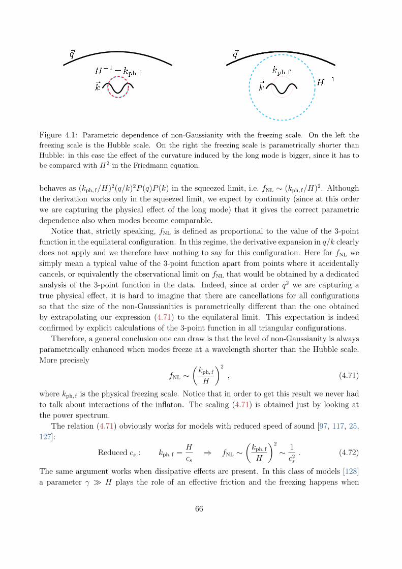
Figure 4.1: Parametric dependence of non-Gaussianity with the freezing scale. On the left the
freezing scale is the Hubble scale. On the right the freezing scale is parametrically shorter than
Hubble: in this case the effect of the curvature induced by the long mode is bigger, since it has to
be compared with H2 in the Friedmann equation.
behaves as (kph, f/H)2(q/k)2P (q)P (k) in the squeezed limit, i.e. fNL ∼ (kph, f/H)2. Although
the derivation works only in the squeezed limit, we expect by continuity (since at this order
we are capturing the physical effect of the long mode) that it gives the correct parametric
dependence also when modes become comparable.
Notice that, strictly speaking, fNL is defined as proportional to the value of the 3-point
function in the equilateral configuration. In this regime, the derivative expansion in q/k clearly
does not apply and we therefore have nothing to say for this configuration. Here for fNL we
simply mean a typical value of the 3-point function apart from points where it accidentally
cancels, or equivalently the observational limit on fNL that would be obtained by a dedicated
analysis of the 3-point function in the data. Indeed, since at order q2 we are capturing a
true physical effect, it is hard to imagine that there are cancellations for all configurations
so that the size of the non-Gaussianities is parametrically different than the one obtained
by extrapolating our expression (4.71) to the equilateral limit. This expectation is indeed
confirmed by explicit calculations of the 3-point function in all triangular configurations.
Therefore, a general conclusion one can draw is that the level of non-Gaussianity is always
parametrically enhanced when modes freeze at a wavelength shorter than the Hubble scale.
More precisely
fNL ∼(kph, f
H
)2
, (4.71)
where kph, f is the physical freezing scale. Notice that in order to get this result we never had
to talk about interactions of the inflaton. The scaling (4.71) is obtained just by looking at
the power spectrum.
The relation (4.71) obviously works for models with reduced speed of sound [97, 117, 25,
127]:
Reduced cs : kph, f =H
cs⇒ fNL ∼
(kph, f
H
)2
∼ 1
c2s
. (4.72)
The same argument works when dissipative effects are present. In this class of models [128]
a parameter γ H plays the role of an effective friction and the freezing happens when
66

c2sk
2/a2 ∼ γH. This implies that Eq. (4.71) reads
Dissipative : kph, f =
√γH
cs⇒ fNL ∼
(kph, f
H
)2
∼ γ
Hc2s
. (4.73)
This matches the explicit calculations of [128]. The argument leading to Eq. (4.71) does
not rely on a linear dispersion relation for the inflaton perturbations and indeed it gives the
correct estimate for Ghost Inflation [100] too, where the dispersion relation is of the form
ω = k2/M . In this case we have
Ghost Inflation : kph, f = (HM)1/2 ⇒ fNL ∼(kph, f
H
)2
∼ M
H. (4.74)
A peculiar example is the one of Khronon Inflation [34]. In this case the power spectrum is
not affected by the background curvature at order 1/c2s since in the quadratic action the scale
factor does not appear at this order and the speed of the inflaton background is immaterial
due to the field redefinition symmetry. Indeed, we check in Appendix A that 1/c2s terms of the
three-point function at order q2 vanish, when the proper angular average is taken. At the end,
let us notice that the general argument above implies that one has completely non-Gaussian
perturbations, i.e. strong coupling, when freezing occurs at a sufficiently short scale
Strong coupling :
(kph, f
H
)2
∼ P−1/2ζ . (4.75)
Some of these arguments can be straightforwardly extended to the trispectrum and higher
correlation functions. For example one can apply twice the argument leading to Eq. (4.70) to
conclude that the amplitude of the four-point function will behave as
τNL ∼(kph, f
H
)4
. (4.76)
This corresponds to 1/c4s for models with reduced speed of sound and (M/H)2 for Ghost
Inflation.
It is worth noticing that our arguments cannot be extended beyond the q2 order. At order
q3 one cannot interpret the three-point function as a calculation of the two-point function on a
long classical background. Indeed, at this order one cannot neglect the time-dependent phase
of the long mode and therefore one cannot describe the long mode classically. Moreover, one
cannot neglect anymore the probability that two short modes combine to give a long one. In
this sense, eq. (4.70) is the last statement we can make treating the long mode as a classical
background.
Let us at the end stress one important point. In the procedure we described above we
are associating non-Gaussianities with the effect of the curvature, by setting the long mode
fluctuation of the inflation to zero with a choice of coordinates. In this way, the interactions
between the long mode and the short modes appear of gravitational origin. On the other hand,
67

we know that the three-point function can also be obtained (up to slow-roll corrections) in
the decoupling limit. In particular, in models with cs 1, freezing happens at scales much
shorter than the curvature and large non-Gaussianities can be understood in flat space. This
simplification is somewhat obscured in the language we use in this Section.
4.4.2 From ζ-gauge to a Curved FRW Universe
In this Section our aim is to show that the long mode, at orderO(q2) is equivalent to a spatially
curved universe. For simplicity, we will neglect the homogenous part and the homogeneous
gradient as they can be always removed by a change of coordinates, and focus only on the
second order in derivative expansion of the long mode
ζL(~x, t) = ζL(t) +1
2∂i∂jζL x
ixj . (4.77)
The time dependence of ζL(~x, t) is fixed by the equation of motion of ζL. Focusing on models
with reduced speed of sound we have
∂t
(εa3
0ζL
)− εa0c
2s ∂
2ζL = 0 , (4.78)
where a0 is the scale factor of the flat FRW universe. Notice that we cannot neglect the time
dependence of ζL since it is of order q2. Substituting eq. (4.77) and solving for ζL(t) at first
order in the slow-roll parameters, we find that the long mode at quadratic order is
ζL(~x, t) = −c2s∂
2ζL2a2
0H20
(1− 2ε) +1
2∂i∂jζL x
ixj . (4.79)
In order to show that at this order the long mode is equivalent to being in a spatially
curved FRW, it is enough to consider the perturbed metric in ζ-gauge at linear order (see for
example [117])
g00 = −1− 2ζLH0
,
g0i = −∂iζLH0
+a2
0ε
c2s
∂iζL∂2
,
gij = a20 (1 + 2ζL) δij ,
(4.80)
and make a gauge transformation to rewrite it in the usual FRW form (i.e. by setting g00 = −1
and g0i = 0). Under the coordinate transformation xµ → xµ = xµ + ξµ(x), the metric
transforms as
g00 = g00 + 2ξ0 ,
g0i = g0i − a20ξi + ∂iξ
0 ,
gij = gij − a20∂iξ
j − a20∂jξ
i − 2a20H0ξ
0δij ,
(4.81)
68

and we can set g00 = −1 and g0i = 0 by choosing the transformation parameters to be
ξ0 =
∫ t
dt′ζLH0
= −c2s∂
2ζL2a2
0H30
(1− 3
2ε
),
ξi = −∫ t
dt′∂iζLa2
0H0
(1− ε) =∂i∂jζLx
j
2a20H
20
. (4.82)
The effect of the long mode is now entirely encoded in the spatial part of the metric
gij = a20
(δij −
∂i∂jζLa2
0H20
+ εc2s∂
2ζL2a2
0H20
δij
)(1 + ∂a∂bζLx
axb), (4.83)
which, once averaged over angles, takes the familiar form
gij, avg=a2
(1− 1
2κx2
). (4.84)
In this expression the spatial curvature κ and the scale factor a in the curved universe are
given by
κ = −2
3∂2ζL , a2 = a2
0
(1 +
κ
2a20H
20
− ε 3c2sκ
4a20H
20
). (4.85)
In conclusion, there are two effects of the long mode at order O(q2). One is to induce the
spatial curvature. The other is to consistently change the scale factor compared to the starting
flat FRW universe. This effect is dominant in the limit of small speed of sound, as we are
going to check in the following Section. Intuitively, the reason is that as cs goes to zero, the
sound horizon where perturbations freeze also shrinks and geometrical effects can be neglected
compared to the effect in the change in the expansion history.
It is important to stress that the change of coordinates (4.82) decays away at late times.
This implies that, since we are interested in correlation functions at late times, that one can
neglect the change of coordinates and just treat the long mode as adding spatial curvature to
the FRW solution. This allows us to write the consistency relation at this order as
〈ζ~qζ~k1ζ~k2〉′q→0, avg=Pζ(q)
2
3· q2 · ∂
∂κ〈ζ~k1
ζ−~k1〉′κ , (4.86)
where the subscript κ means that the two-point function is calculated in the curved universe.
As before, the assumption used to derive this formula is the fact that the background solution
is on the attractor, so that the time-dependence of the long mode ζL starts at order q2.
Notice that in deriving eq. (4.85) we used the slow-roll approximation, but we expect the
relationship to hold at all orders in the slow-roll expansion. Our consistency condition should
indeed hold for all FRW backgrounds that are accelerating so that modes freeze after horizon
crossing. This implies that the effect of the long mode on the short ones is captured by a
derivative expansion of the long mode at the time when the short modes cross the horizon.
69

One can generalize these arguments without taking the angular average and consider a curved
anisotropic (but homogeneous) universe. In this case eq. (4.86) becomes
〈ζ~qζ~k1ζ~k2〉′q→0 = Pζ(q) qiqj
∂
∂(qiqjζ~q)〈ζ~kζ−~k〉′local , (4.87)
where 〈. . . 〉local means that the two-point function is calculated in a locally anisotropic curved
universe.
4.4.3 Checks
As we already pointed out, eq. (4.86) is not the consistency relation in the usual sense,
because it relates correlation function calculated in two different universes. One of them is
flat and the other has a spatial curvature κ. Therefore, in order to check eq. (4.86), one has
to calculate correlation functions in the curved universe. This is not so easy, in particular
because of the geometrical effects (for example, one cannot expand the modes in plane waves).
Furthermore, to do the comparison with the three-point function, the two-point function in
the curved universe must be expressed in terms of the flat universe parameters (for example
speed of sound cs). Luckily, at least in some regimes, some of these difficulties are not
present. For example, if we take a parametric limit cs 1, then the modes freeze at scales
much smaller than the curvature scale, and one can neglect geometrical effects and work in
the approximation of a flat space. The only way the curvature enters the problem is through
the change of the expansion rate as described in (4.85).
Let us therefore focus on the models with small speed of sound and check eq. (4.86) at
leading order in 1/c2s. The simplest way to do the check is to use the action for K-inflation in
the decoupling limit in a curved universe (see for example [97])
S =
∫d4x√−gP (X,φ) , (4.88)
where X = −12gµν∂µφ∂νφ. For the homogeneous background φ(t) this action boils down to
S =1
2
∫d4x
(a3PX φ
2 − a3V (φ)), (4.89)
and the corresponding equation of motion is
∂t(a3PX φ)− a3V ′ = 0 . (4.90)
This equation implies that the effect of curvature is not only to change the scale factor. If
we perturb a(t), to be consistent we also have to change the background field φ(t). To find
what change in the field compared to the flat universe comes from adding curvature, let us
first write down the equation of motion in the following way
PX φ+ 3HPX φ+ 2PXXXφ = −V ′ . (4.91)
70

Now we can split the background in the part which corresponds to the evolution in a flat
universe, and a small perturbation coming from curvature: φ = φ0+δφ. Using the background
equation of motion for φ0, we find that the small perturbation δφ has to satisfy
2PXXXδφ+ 6H0φ20PXXδφ+ 3PX φ0δH = 0. (4.92)
Using the change of the scale factor in the presence of curvature eq. (4.85), one can easily
find the change of the Hubble constant δH. The equation of motion for δφ becomes
δφ+ 3H0δφ =3
2c2sH0φ0
R
a20H
20
, (4.93)
and the solution is simple to find
δφ = C a−30 +
3
2c2sφ0
R
a20H
20
. (4.94)
The homogeneous part decays faster than the particular solution and we can neglect it.
To summarise, in models with the small speed of sound, the leading effect of the long
mode is to change the background evolution. This change affects the inflation speed as well,
that has to be consistently shifted by the amount we calculated above. The relative changes
of the relevant quantities are
δa(η)
a(η)=κ
6η2 and
δX
X= 2
δφ
φ= 3
c2sκ
H20a
20
. (4.95)
Let us now turn back to the problem of calculating the power spectrum of perturbations
in the presence of the curvature κ. We can start from the action for perturbations [97]
S =1
2
∫d4x√−g
((XPX + 2X2PXX)π2 −XPXgij∂iπ∂jπ + 3κXPXπ
2), (4.96)
and vary all relevant quantities. For example
PX → PX
(1 +
XPXXPX
δX
X
), PXX → PXX
(1 +
XPXXXPXX
δX
X
). (4.97)
Using the definition for the parameters c2s, λ and Σ of Ref. [117],
XPXXPX
=1
2
(1
c2s
− 1
),
2X2PXXXPX
=3λ
c2sΣ− 3
2
(1
c2s
− 1
), (4.98)
the action in Eq. (4.96) reads
S =
∫d4x H2
0 εa20
[1
c2s
(1 +
κ
3a20H
20
+9c2sκ
a20H
20
λ
Σ
)π′
2 −(
1 +11κ
6a20H
20
)(∂iπ)2
]. (4.99)
71

Here we are considering only terms which contribute at order 1/c2s. This greatly simplifies the
calculation since the metric can be taken to be spatially flat and the field can be decomposed
in Fourier modes. The equation of motion derived from this action is
π′′~k −2
ηπ′~k + c2
sk2π~k +
κ
a20H
20
((1
3+ 9c2
s
λ
Σ
)π′′~k +
11
6c2sk
2π~k
)= 0 , (4.100)
and can easily be solved perturbatively in κ. Once the solution has been properly normalised,
the power spectrum for ζ can be calculated using the standard procedure. The final result is
〈ζ~kζ−~k〉′κ = Pζ(k)
(1− 19 + 18 λ
Σ
8c2sk
2κ
). (4.101)
The contribution to the squeezed limit of the three-point function is then obtained by aver-
aging over the long mode and substituting κ = 23q2ζ~q
〈ζ~qζ~k1ζ~k2〉′q→0 = −Pζ(q)Pζ(k)
1
c2s
(19
12+
3
2
λ
Σ
)q2
k2. (4.102)
Indeed, this agrees with the squeezed limit of the three-point function at second order in q,
once the angular average is taken and terms not enhanced by 1/c2s are neglected (see Appendix
A). For a more detailed discussion, involving checks with anisotropic long mode and including
geometrical effects, see [126].
4.5 Multiple Soft Limits
All consistency relations we discussed so far involve a correlation function with a single soft
external momentum. It is possible to generalize the consistency relations to cases when
multiple external momenta are taken to be soft. In this Section we are going to give a few
most important results and highlight some of the problems one encounters trying to derive the
consistency relations for the multiple squeezed limit. We are also going to focus on scalars.
The full derivation of all results is beyond the scope of this thesis and more details can be
found in [129].
The way to get the consistency relations with multiple soft external legs is essentially
the same as for the single soft mode. The long mode ζL is locally equivalent to a change of
coordinates and we can write
〈ζ(x1) · · · ζ(xn)|ζL〉 = 〈ζ(x1) · · · ζ(xn)〉 . (4.103)
To get the the correlation function with multiple soft modes we have to multiply this equality
with ζ(y1) . . . ζ(ym) and average over the long modes. Notice that in order to be consistent, we
also have to expand the right hand side up to order O(δxm). This is an important difference
compared to the case of a single soft mode. For multiple soft limit it is impossible to linearize
the change of coordinates.
72
In the following sections we are going to sketch the derivation of the consistency relations
with two soft modes at different orders in the gradient expansion. This simplified problem
still captures all the subtleties of the derivation. At the end, we will present a check of these
relations in models with small speed of sound.
Before we proceed, let us write down the exact (not infinitesimal) change of coordinates
that corresponds to a dilation and a special conformal transformation (see, e.g., [130])
xi → eλxi , (dilation)
xi → xi − bi~x2
1− 2~x ·~b+ ~x2~b2. (SCT) (4.104)
Under these transformations, the spatial part of the line element transforms as
δijdxidxj → Ω2(~x)δijdx
idxj , (4.105)
where the conformal pre-factor is given by
Ωdil(~x) = eλ ,
ΩSCT(~x) = (1− 2~x ·~b+ ~x2~b2)−1 . (4.106)
So far we were using only linearised versions of these equations, but in the following sections
will need non-linearised expressions to derive consistency relation with multiple soft momenta.
4.5.1 Zeroth Order in Gradients
Let us first look at the simplest case of homogeneous long modes. As we said, for simplicity, we
will consider two soft modes, which requires working at quadratic order in ζL. The nonlinear
ζL is generated by a finite dilation of the spatial coordinates
xi → eζL(~x+)xi . (4.107)
Notice that this is a simple generalisation of eq. (4.8). This implies that the variation of
coordinates, up to second order in ζL, is given by
δxi = xi − xi '(ζL +
1
2ζ2L
)xi . (4.108)
Given this setup, the derivation proceeds in the same way as in Section 4.1. After going
to momentum space, commuting derivatives through delta functions and many integrations
by parts [129], one finds that the variation of an n-point function is given by
δ〈ζ~k1· · · ζ~kn〉
′ = lim~q→0
(−ζ~q δ(n)
D +1
2
∫d3Qζ~qζ ~Q−~q (δ
(n)D )2
)〈ζ~k1· · · ζ~kn〉
′ , (4.109)
where δ(n)D is just the dilation operator
δ(n)D = 3(n− 1) +
n∑a=1
kai∂kai . (4.110)
73

Notice that there are two different terms in the variation of the n-point function. They
correspond to two different contributions to the double squeezed limit of the (n + 2)-point
function. Indeed, if we average the previous relation over ζ~q1ζ~q2 , we finally get
lim~q1,~q2→0
〈ζ~q1ζ~q2ζ~k1· · · ζ~kn〉
′ = −〈ζ~q1ζ~q2ζ−~q〉′δ(n)D 〈ζ~k1
· · · ζ~kn〉′ + Pζ(q1)Pζ(q2)(δ
(n)D )2〈ζ~k1
· · · ζ~kn〉′ .
(4.111)
The first term in (4.111) describes two soft modes combining and linking to the hard modes
via a soft internal line. This causes the diagram to factorize into a three-point function with
no hierarchy between the modes and an n-point function rescaled by the presence of a long
internal line. The second term in (4.111) corresponds to the case where both soft lines come
from a single vertex (the contact diagram), which induces a double dilation on the remaining
hard modes. Equation (4.111) is a generalization of Maldacena’s consistency relation for a
single soft external leg. It was first considered in [131, 132] and derived in this form in [129]4.
It is important to stress that in some cases these two terms may be of different orders
in slow-roll parameters, such that one is suppressed compared to the other. For example,
in single-field models with reduced speed of sound, the three-point function is not slow-roll
suppressed, while the second term is higher-order in slow-roll parameters. This is not a
generic case. For instance, in standard slow-roll inflation both terms are expected to be
equally relevant (second order in slow-roll parameters). One can also find examples where
the second term is dominant. This happens in the case of resonant non-Gaussianities, where
diagrams with more vertices are always subdominant [119].
The other way to see that one needs both terms in (4.111) is to look at the hierarchical limit
q1 q2. Physically, this corresponds to a situation where the mode with the wavenumber ~q1
goes outside the horizon much before all the others. After that, the other mode ~q2 becomes
longer than the horizon and eventually short modes cross it too. Intuitively, in this kind
of situation, to get the double soft limit of an (n + 2)-correlation function, we can apply
Maldacena’s consistency relation twice in the following way
lim~q1~q2→0
〈ζ~q1ζ~q2ζ~k1· · · ζ~kn〉
′ = Pζ(q1)δ(n+1)D
(Pζ(q2)δ
(n)D 〈ζk1 · · · ζkn〉′
). (4.112)
Indeed, this is exactly what we find from eq. (4.111). In the limit q1 q2 we have
lim~q1~q2→0
〈ζ~q1ζ~q2ζ~k1· · · ζ~kn〉
′ = Pζ(q1)δ(2)D Pζ(q2) δ
(n)D 〈ζk1 · · · ζkn〉′ + Pζ(q1)Pζ(q2)(δ
(n)D )2〈ζk1 · · · ζkn〉′
= Pζ(q1)δ(n+1)D
(Pζ(q2)δ
(n)D 〈ζk1 · · · ζkn〉′
). (4.113)
Notice that we have additional terms in the dilation operator when it acts on modes with
momentum q2.
4Notice that in [131, 132] the consistency relation contained only the first term on the right-hand side
of (4.111).
74

4.5.2 First Order in Gradients
In this Section we will extend the discussion about consistency relations with two soft modes
beyond the homogeneous limit and keep the first order corrections in gradients. Up to second
order in ζL and first order in the gradient expansion, the spatial line element is given by
d~l2 = a2(t)e2ζL(~x)d~x2
' a2(t)
(1 + 2ζL + 2ζ2
L + 2~x · ~∇ζL + 4ζL~x · ~∇ζL)
d~x2 , (4.114)
where we have expanded the long mode around the origin
ζL(x) = ζL + ~x · ~∇ζL + · · · . (4.115)
It is obvious that the change of coordinates that generates the long adiabatic mode at
this order must involve one dilation and one special conformal transformation. However, it is
well known that these two transformations do not commute. Therefore, one can be confused
about the order in which these two transformations should be performed. For example, in
the case of internal symmetries, taking multiple soft limits in different orders gives different
answers. It turns out that different ordering of limits is related to the commutators of broken
generators, allowing to probe the structure constants of the algebra of broken generators
experimentally (see for example a discussion in [133]). On the other hand, in case of inflation,
the only Goldstone boson is ζ and the correlation functions are symmetric, such that taking
limits in different order gives always the same answer.
This is not a paradox, because it turns out that the order of transformations that induce the
long mode is not arbitrary. It is fixed by demanding that the change of coordinates generates
a physical solution, corresponding to the spatial line element (4.114). Indeed, using (4.106),
we can see that doing a special conformal transformation first gives5
(D SCT)d~x2 =(
1 + 2λ+ 2λ2 + 4~b · ~x+ 12λ~b · ~x+ · · ·)
d~x2 , (4.116)
while if we do the transformations in opposite order we get
(SCT D)d~x2 =(
1 + 2λ+ 2λ2 + 4~b · ~x+ 8λ~b · ~x+ · · ·)
d~x2 . (4.117)
Comparing these expressions with (4.114), we see that only (4.117) can be consistently
matched with the physical solution if we choose λ and ~b in the standard way
λ = ζL , ~b =1
2~∇ζL . (4.118)
Notice that the difference between eq. (4.116) and eq. (4.117) is just 4λ~b · ~x. This reflects the
fact that the commutator of generators for dilations and special conformal transformations is
proportional to the generator of special conformal transformations.
5Here we work at linear order in ~b, but keep terms of order λ~b and λ2. The reason is that λ ∼ ζL and~b ∼ ~∇ζL, and we want to keep terms that are first order in gradients but second order in ζL.
75

The summary of this discussion is that, in order to generate the line element (4.114)
corresponding to a physical solution, we must do a dilation first and then perform a special
conformal transformation. The full change of coordinates (up to an irrelevant spatial trans-
lation) that is equivalent to a physical long mode up to second order in ζL and first order in
derivatives is
δxi =
(ζL +
1
2ζ2L + (1 + ζL) ~x · ~∇ζL
)xi − 1
2(1 + ζL) ~x2∇iζL . (4.119)
To get the consistency relation one can follow the same steps as before. Here we will just
quote the final result. For more details and some other technical steps in the derivation, see
[129]. After we consistently expand the variation of an n-point function to second order in
ζL, go to momentum space, average over ζ~q1ζ~q2 and do a lot of integrations by parts, the final
result is
lim~q1,~q2→0
〈ζ~q1ζ~q2ζ~k1· · · ζ~kn〉′
Pζ(q1)Pζ(q2)= − 〈ζ~q1ζ~q2ζ−~q〉
′
Pζ(q1)Pζ(q2)δ
(n)D 〈ζ~k1
· · · ζ~kn〉′ + (δ
(n)D )2〈ζ~k1
· · · ζ~kn〉′
+1
2qi1
(δ
(n)
Ki δ(n)D 〈ζ~k1
· · · ζ~kn〉′ − 〈ζ~q1ζ~q2ζ−~q〉
′
Pζ(q1)Pζ(q2)δ
(n)
Ki 〈ζ~k1· · · ζ~kn〉
′), (4.120)
where, as before, δ(n)
Ki is the operator of the special conformal transformation in momentum
space
δ(n)
Ki =n∑a=1
(6∂kai − kai∂2
ka + 2~ka · ~∂ka∂kai). (4.121)
Notice that the first line matches the result (4.111) in the homogeneous limit, while the second
line contains gradient corrections.
4.5.3 Second Order in Gradients
From what we described so far, it might seem that going to higher order in gradients is
straightforward. One always has to make sure to expand the conformal factors (4.106) to
a given order in q and ζL and to use the change of coordinates that matches the physical
solution in ζ-gauge. However, already at second order in gradients, we meet a problem. We
already saw that the effects of a single long mode at order O(q2) are physical and cannot
be removed by a change of coordinates. It turns out that the same happens if we want to
consider two long modes, each at linear order in gradients, even though they individually
locally act only as a coordinate transformation.
The intuitive reason for this somewhat surprising result is the following. Imagine that we
want to calculate the squeezed limit of an (n + 2)-point function and keep the corrections
of order O(q1q2). Some contributions to the result will come from diagrams where the two
long modes combine to a single soft internal line. As we already saw, this kind of diagrams
factorise to the three-point function 〈ζ~q1ζ~q2ζ~q〉′ and the (n+ 1)-point function 〈ζ−~qζ~k1. . . ζ~kn〉′.
Therefore, in order to capture corrections of order O(q1q2), we unavoidably have to deal with
76

the effects of the soft internal mode on the remaining n hard modes that are of the order
(~q1 + ~q2)2. But this is exactly the effect of the curvature of the long mode, and cannot be
calculated using just the coordinate transformation.
The other way to see this problem is the following. Given that we are interested in the
construction of the adiabatic mode at order (∇ζL)2, we expect that the change of coordinates
we need to do is a special conformal transformation at second order in ~b2. However, one can
explicitly check that the second order conformal transformation does not match the physical
long mode. The reason is that at second order in q and ζ~q one has to take into account the
term ζL∇2ζL that is related to the curvature of the long mode. Indeed, neglecting dilations
for simplicity, the difference between the line element with a physical long mode and the
conformal transformation is
e2~x·~∇ζL+xixj∇i∇jζL − Ω2sct
∣∣bi=
12∇iζL
= xixj∇i∇jζL +(~x · ~∇ζL
)2
− 1
2~x2(~∇ζL
)2
. (4.122)
This is not so surprising. One way to understand this difference is that for the physical long
mode the spatial curvature at order we are interested in is proportional to R(3) ∼ q2ζ2~q , while
the special conformal transformation leaves the space flat, at any order in ~b.
Despite these issues, it is still possible to write down a relation among the correlation
functions that is correct at order O(q1q2). The details of the calculation are rather technical,
and we will not present them here (the interested reader can find it in [129]). Let us just
quote the final result and comment on some of the terms. For two soft modes we get
limq1,q1→0
1
Pζ(q1)Pζ(q2)〈ζq1ζq2ζk1 · · · ζkn〉′ = −
〈ζq1ζq2ζ−q〉′Pζ(q1)Pζ(q2)
(δ
(n)D +
1
2~q · δ(n)
~K
)〈ζk1 · · · ζkn〉′
+
((δ
(n)D )2 +
1
2~q · δ(n)
~Kδ
(n)D +
1
4qi1q
j2δ
(n)
Ki δ(n)
Kj
)〈ζk1 · · · ζkn〉′
+ limq→0
[1
2(~q2∇2
q − 2qiqj∇iq∇j
q)〈ζqζk1 · · · ζkn〉′
+〈ζq1ζq2ζ−q〉′Pζ(q1)Pζ(q2)
qiqj∇iq∇j
q
1
P (q)〈ζqζk1 · · · ζkn〉′
]. (4.123)
The first two lines in this expression contain what one would naively have guessed using
the consistency relations with a single soft momentum. The first line describes the effect of
a soft internal mode that comes from two long modes on the n-point function. The second
line is a “square” of the sum of the dilation and the special conformal operator. On the other
hand, the last two lines come from the effects of the curvature of the long mode. They are
obtained using the arguments behind eq. (4.86). One can see that these terms correspond to
the mismatches in eq. (4.122). The first line comes from the last two terms in eq. (4.122),
while the last line comes from the first term.
The main importance of this result is to show that at higher orders in ∇ζL, even though
each gradient is locally just a change of coordinates, when they combine their total effect
has a physical part. This makes the extension to higher orders in gradients even harder.
77

Let us also stress one limitation of eq. (4.123). For example, in simple single-field slow-roll
inflation, two scalar modes can combine to give a tensor mode. In principle, this can be also
captured in the expression for the double squeezed limit. Therefore, our choice to neglect
the contribution from tensor modes constrains the applicability of eq. (4.123) only to some
situations, for example models with small speed of sound where we can work in the decoupling
limit.
Let us finally notice that if we are interested only in homogeneous long modes, we can
apply the procedure described above for an arbitrary number of soft external legs. As we will
see later, the same is true in the context of the Newtonian limit of the consistency relations
of LSS. We will come back to some of the issues presented here in Section 5.2.2.
4.5.4 Checks
In this Section we will perform a check of the consistency relations with two soft external
modes using correlation functions calculated in models with small speed of sound. We must
consider at least a four-point function on the left hand side. On the right hand side most
of the terms vanish, because the two-point function is both scale and conformally invariant.
The only nontrivial contributions are at order O(q1q2). The consistency relation in this case
boils down to
lim~q1,~q2→0
∇jq1∇iq2
(〈ζ~q1ζ~q2ζ~k1ζ~k2〉′
Pζ(q1)Pζ(q2)
)= lim
~q→0
[1
2δij∇2
q +
( 〈ζ~q1ζ~q2ζ−~q〉′Pζ(q1)Pζ(q2)
− 1
)∇iq∇j
q
] 〈ζ~qζ~kζ−~k〉′Pζ(q)
.
(4.124)
Let us calculate the contributions on the two sides of the consistency relation.
On the left hand side, there are two types of diagrams that contribute to the four-point
function (see Appendix A). In the double-squeezed limit, the contact contribution gives
lim~q1,~q2→0
〈ζ~q1ζ~q2ζ~k1ζ~k2〉′cont. = Pζ(q1)Pζ(q2)Pζ(k)
(1− 1
c2s
)(3
4
~q1 · ~q2
k2+
5
2
(~k · ~q1)(~k · ~q2)
k4
).
(4.125)
Notice that for simplicity we set λ = 0 in all calculations. The exchange diagram is expected
to factorize
lim~q1,~q2→0
〈ζ~q1ζ~q2ζ~k1ζ~k2〉′exc. = lim
~q→0〈ζ~q1ζ~q2ζ−~q〉′
〈ζ~qζ~k1ζ~k2〉′
Pζ(q). (4.126)
Assuming scale invariance, the last factor vanishes up to O(q2) by the usual consistency
relations. At order q2, however, we have the effects of the curvature of the long mode ζ~q
lim~q→0〈ζ~qζ~k1
ζ~k2〉′ = Pζ(q)Pζ(k)
(1− 1
c2s
)(2q2
k2− 5
4
(~k · ~q)2
k4
). (4.127)
Substituting into (4.126), the exchange contribution becomes
lim~q1,~q2→0
〈ζ~q1ζ~q2ζ~k1ζ~k2〉′exc. = Pζ(k)
(1− 1
c2s
)(2q2
k2− 5
4
(~k · ~q)2
k4
)〈ζ~q1ζ~q2ζ−~q〉′ . (4.128)
78

Now we can calculate the left hand side of the consistency relation. Taking derivatives with
respect to q1 and q2, we obtain6
lim~q1,~q2→0
∇jq1∇iq2
〈ζ~q1ζ~q2ζ~k1ζ~k2〉′
Pζ(q1)Pζ(q2)= Pζ(k)
(1− 1
c2s
)[(3
4
δij
k2+
5
2
kikj
k4
)+
(4δij
k2− 5
2
kikj
k4
) 〈ζ~q1ζ~q2ζ−~q〉′Pζ(q1)Pζ(q2)
]. (4.129)
To compare this to the right hand side of (4.124), we need the three-point function with
λ = 0 (see Appendix A)
〈ζ~k1ζ~k2ζ~k3〉′ = Pζ(k2)Pζ(k3)
1
2k31
[(1
c2s
− 1
)12k2
1k22k
23
k3t
+
(1
c2s
− 1
)(− 8
kt
∑i>j
k2i k
2j +
4
k2t
∑i 6=j
k2i k
3j +
∑i
k3i
)], (4.130)
where kt = k1 + k2 + k3. Using this, we obtain
lim~q→0∇iq∇j
q
〈ζ~qζ~kζ−~k〉′P (q)
= Pζ(k)
(1− 1
c2s
)(4δij
k2− 5
2
kikj
k4
). (4.131)
This leads to the following expression for the right-hand side of (4.124)
lim~q→0
[1
2δij∇2
q +
( 〈ζ~q1ζ~q2ζ−~q〉′Pζ(q1)Pζ(q2)
− 1
)∇iq∇j
q
] 〈ζ~qζ~kζ−~k〉′Pζ(q)
= Pζ(k)
(1− 1
c2s
)[(3
4
δij
k2+
5
2
kikj
k4
)+
(4δij
k2− 5
2
kikj
k4
) 〈ζ~q1ζ~q2ζ−~q〉′Pζ(q1)Pζ(q2)
], (4.132)
which precisely agrees with (4.129).
4.6 Consistency Relations as Ward Identities
In this Chapter we presented the derivation of the inflationary consistency relations based
on the fact that the long mode (scalar or tensor) locally acts only as a rescaling of coordi-
nates. There is another way to obtain the same result and it is based on Ward identities
for spontaneously broken space-time symmetries. Indeed, in ζ-gauge, the co-moving curva-
ture perturbation ζ can be thought of as the Goldstone boson of the spontaneously broken
space-time symmetry
SO(4, 1) → R3 × SO(3) . (4.133)
In this gauge there remain residual large gauge transformations under which ζ transforms
non-linearly. These transformations are dilations and special conformal transformations [134].
The quantum-mechanical consequences of these symmetries are Ward identities which relate
6The second term gets a factor of 2 from the fact that q2 ⊃ 2~q1 · ~q2.
79

correlation functions with a soft external line to a lower point function, leading exactly to the
inflationary consistency relations [50, 51].
We will not enter the details of the derivation of the consistency relations using Ward
identities. Given that this approach attracted some attention in the literature, in this Section
our goal is just to very briefly highlight the main results and compare them with what we did
so far. Before we move to the full theory including gravity, we will first focus on the simpler
case of the decoupling limit.
4.6.1 Decoupling Limit
In the decoupling limit we can neglect the effects of gravity, which makes the discussion much
simpler. Inflation takes place in an approximate de Sitter space
ds2 = −dt2 + e2Htd~x2 , (4.134)
a maximally symmetric space whose isometry group is SO(4, 1). Notice that this coincides
with the group of conformal transformations in 3-dimensional Euclidean space. The time-
evolving inflaton background is homogeneous and rotationally invariant, so that translations
and rotations are exact symmetries of the whole system and show up in an obvious way at
the level of correlation functions. This accounts for 6 out of the 10 generators of SO(4, 1).
The other 4 generators are related to the dilation isometry
t→ t−H−1 log λ , ~x→ λ~x , (4.135)
and another isometry
t→ t− 2H−1~b · ~x , xi → xi − bi(−H−2e−2Ht + ~x2) + 2xi(~b · ~x) , (4.136)
parametrized by the infinitesimal vector ~b, that at large times t → +∞, act on the spatial
coordinates as special conformal transformations. None of these transformations, on general
grounds, are symmetries of the inflaton background. Indeed the solution—which we can
always assume to be of the form φ = t by a suitable field redefinition—is not invariant under
a time shift.
However, in inflationary models it is quite common that there is an additional (approx-
imate) symmetry, the shift symmetry φ → φ + c. In this case the inflaton background is
invariant under a combination of a dilation and a shift of the field7. As we saw in the In-
troduction, this unbroken symmetry is the origin of the approximate scale-invariance of the
inflationary correlation functions [60]. The obvious question is whether a similar thing can
happen for other isometries. One may wonder whether it is possible, like in the case of dila-
tions, to impose an additional symmetry on the inflaton Lagrangian in such a way that some
7One can also consider the case in which the system is only invariant under a discrete (and not continuous)
shift symmetry, see [120].
80

combination of the isometries (4.136) and this internal symmetry is preserved. This would
require that the inflaton action is invariant under
φ→ φ+~b · ~x , (4.137)
so that it is possible to cancel the variation induced on φ by the isometries (4.136). Notice
that this is a Galilean transformation [135] with a spatial transformation parameter. It is
certainly possible to write an inflaton action which is Galilean invariant [136, 35], but it is
well known that this symmetry is only well defined in the Minkowski limit and broken by a
curved background [137]. This implies that correlation functions, which probe the theory at
a scale comparable with the curvature, cannot be invariant under the isometries (4.136) 8.
The fact that some of the isometries are spontaneously broken must be reflected at the
level of the correlation functions. Indeed, in QFT, one can always write down Ward identities
for non-linearly realised symmetries. These are non-perturbative results that relate the soft
limits of an (n+1)-point correlation function to an appropriate variation of the corresponding
n-point function. It turns out that Ward identities for spontaneously broken dilations and
special conformal transformations have exactly the form of the consistency relations.
Let us take a closer look at the derivation of the consistency relation in the decoupling
limit. We will start by expanding the long-wavelength mode to linear order in ~x
πL(x) = πL(0) + ∂iπL(0)xi. (4.138)
The constant piece πL(0) can be induced by a rescaling of coordinates which, in the presence
of a shift symmetry, leaves the correlation functions invariant. We will focus on the linear
piece ∂iπL(0)xi. Let us write down the transformation of the perturbations under a special
conformal transformation, eq. (4.136), parametrized by the infinitesimal parameter ~b
π(x)→ π(x) = π(x) + 2H−1~b · ~x . (4.139)
According to this relation a constant gradient can be induced by a special conformal trans-
formation on the coordinates with ~b = −(1/2)H~∂πL(0) (9)
〈π(~x1) . . . π(~xn)〉∂πL = 〈π(~x1) . . . π(~xn)〉 , (4.140)
where xi ≡ xi − bi~x2 + 2xi(~b · ~x). This equation holds in the out-of-the-horizon limit, when
one can drop the time-dependent piece in the transformation of the xi in the isometry (4.136)
8In exact de Sitter and in the decoupling limit, interactions of the form (φ)n are invariant under spatial
Galilean transformations. However, it is easy to check that all these couplings are redundant, i.e. they can be
set to zero by a proper field redefinition. This field redefinition is of the schematic form φ→ φ+ (φ)n−1 and
thus vanishes on large scales, giving trivial cosmological correlation functions. Correlation functions are not
trivial on short scales and are obviously SO(4, 1) invariant because they are produced by a de Sitter invariant
field redefinition.9The long wavelength mode is taken to be time-independent: we are implicitly assuming that its time-
dependence arises at O(k2) and can thus be neglected for our purposes.
81
and neglect the time-dependence of π. The variation of the correlation function under such a
coordinate transformation is not zero and will therefore induce a relation between the variation
of the n-point function and the squeezed limit of the (n + 1)-point function. Let us proceed
by computing this variation in Fourier space
δ〈π(~x1) . . . π(~xn)〉 =
∫dKn〈π~k1
. . . π~kn〉(−i)n∑a=1
kia
[bi~x2
a − 2xia(~b · ~xa)
]ei(
~k1·~x1+···+~kn·~xn)
=
∫dKne
i(~k1·~x1+···+~kn·~xn)(−i)n∑a=1
bi(
6∂kia − kia~∂2ka + 2~ka · ~∂ka∂kia
)〈π~k1
. . . π~kn〉 . (4.141)
We can thus compute the (n+ 1)-point correlation function where one of the modes is much
longer than the other n to linear order in the gradient of the long mode
〈π~qπ~k1. . . π~kn〉~q→0 =
⟨π~q〈π~k1
. . . π~kn〉πL⟩
= (−i)〈π~qbi〉′n∑a=1
(6∂kia − kia~∂2
ka + 2~ka · ~∂ka∂kia)〈π~k1
. . . π~kn〉
=H
2Pπ(q)qi
n∑a=1
(6∂kia − kia~∂2
ka + 2~ka · ~∂ka∂kia)〈π~k1
. . . π~kn〉 , (4.142)
where in the second equality we used the fact that a constant mode leaves the correlation
functions unaffected in the presence of the field shift symmetry. Since within the approxima-
tions used in this Section one can relate the curvature perturbation in comoving gauge ζ with
the field perturbation by ζ = −Hπ, we rewrite this last equation as10
〈ζ~qζ~k1. . . ζ~kn〉
′~q→0 = −1
2P (q)qi
n∑a=1
(6∂kia − kia~∂2
ka + 2~ka · ~∂ka∂kia)〈ζ~k1
. . . ζ~kn〉′ , (4.143)
where P is the power-spectrum of ζ. This is exactly the consistency relation (4.28) in the
limit of the exact scale invariance. However, here we derived it as a consequence of the
spontaneously broken de Sitter isometries. One should not be surprised that we get the same
result. At the end of the day, we are asking the same question about the behaviour of the
squeezed limits of correlation functions in both approaches.
Let us at the end stress one technical point. Typically, when a symmetry is broken spon-
taneously, the number of Ward identities is equal to the number of broken generators. This
is the case for the consistency relation too. If we count zeroth order in q and there identi-
ties proportional to qi as independent, then indeed we see that we have four Ward identities
for the four broken generators (one dilation and three special conformal transformations).
However, notice that we have only one Goldstone boson π. Indeed, for spontaneously broken
space-time symmetries, it is well known that the number of Goldstone bosons is not the same
as number of broken generators (see for example [42]).
10Here we used the fact that δ(~q + ~k1 + · · ·+ ~kn) ≈ δ(~k1 + · · ·+ ~kn) up to subleading corrections in q, and
that the transformation commutes with the Dirac delta up to vanishing terms proportional to the dilation of
the n-point function.
82

4.6.2 Ward Identities
In the previous Section we saw that that, in the decoupling limit, consistency relations can
be thought of as Ward identities of spontaneously broken de Sitter isometries. Remarkably,
this can be extended to include gravity, as shown in a series of papers [49, 50, 51, 53, 54].
Let us here very briefly present the main logic of the derivation. The starting point is
a realisation that once the comoving gauge is fixed, the co-moving curvature perturbation ζ
non-linearly realises dilations and special conformal transformations [134]. More generally,
even in the presence of short gravitons, the spatial metric in ζ-gauge
hij = a2e2ζ (eγ)ij , (4.144)
is invariant under simultaneous particular change of spatial co-ordinates and shift in fields
ζ and γ. These change of co-ordinates are residual diffeomorphisms that do not fall off at
infinity and they leave the form of the metric (4.144) unchanged. The fact that they diverge
at infinity is not necessarily a problem11. It turns out that one can generalize Weinbergs
argument [44] to show that some linear combinations of the transformations can be smoothly
extended to physical solutions that have a regular behaviour. As before, these transformations
then correspond to adiabatic long modes. Finally, the last step is to derive Ward identities
for this residual gauge symmetry.
Without entering the further details, let us just quote the main result of this approach.
Schematically, one can write down (see for example [50])
limq→0
Mm∇mq
(1
Pζ(q)〈ζqA(~k1, · · · , ~kn)〉+
1
Pγ(q)〈γqA(~k1, · · · , ~kn)〉
)∼Mm∇m
k 〈A(~k1, · · · , ~kn)〉 ,(4.145)
where A(~k1, · · · , ~kn) is an arbitrary operator built out of tensor and scalar perturbations.
Notice that eq. (4.145) seems to suggest that there are infinitely many identities, one at each
order in q. On the other hand, from the discussion in Section 4.4, we know that at second
order in gradient expansion the long mode has some physical effects on the short modes. The
resolution to this apparent paradox is that the Mm are projection tensors, which only partially
constrain the soft limit of the amplitude at each order O(qm) for m ≥ 2.(12) The part that
can be constrained at higher orders in q is related to long tensor modes. For m = 0 and
m = 1, one recovers the standard Maldacena and conformal consistency relations.
Notice that one of the major advantages of using the Ward identities approach to con-
sistency relations is that it automatically incorporates the situations in which one has short
tensor modes in the correlation functions. As we discussed in Section 3.3.3 and Section 4.2,
this is not automatic in the approach described in this thesis. Another important point is
that Ward identities are exact to all orders in perturbation theory and including quantum
mechanical effects [49, 50, 51]. On the other side, the derivation of the consistency relation
using the equivalence of the long mode and the change of co-ordinates relies on treating the
11We already discussed this issue in Chapter 3.12For recent checks of these relations, see [138].
83

long mode as a classical background. Although we already claimed that the consistency re-
lations must hold non-perturbatively, the agreement with Ward identities approach is a nice
check.
84
Chapter 5
Consistency Relations of Large Scale
Structure
During inflation vacuum fluctuations are stretched by the exponential expansion of space. In
single-field models, once the modes are outside the horizon, they remain frozen and in the
region of space much smaller than their wavelength they are indistinguishable from a rescaling
of coordinates. Once inflation is over, the modes start to enter back into the Hubble radius
and became observable. It is therefore interesting to ask whether the long mode can be seen
locally as change of coordinates even when it is inside the horizon. The relevant quantity
to answer this question, as we saw in Chapter 3, is the sound horizon, because it sets the
length scale above which the interactions cannot propagate within a Hubble time. Before
the decoupling of photons the sound horizon is almost the same as the Hubble scale, but
after that it practically shrinks to zero. All modes that enter the Hubble horizon after the
decoupling and that we can observe nowadays are indeed just a coordinate redefinition on
scales sufficiently small compared to their wavelength.
In Chapter 3 we showed how one can add a long mode to a short-scale solution of the
Einstein’s equations just by performing a change of coordinates and generate in this way a
new solution. We saw that this is possible both in inflation and in the late universe. Of
course, if we want to use this trick to make contact with observations, we have to find a
way to reformulate this statement on terms of correlation functions. In Chapter 4 we studied
how the construction of the adiabatic modes allows us to derive consistency relations for
single-field inflation. In this Chapter, we will turn to the late universe and show that for
the correlation functions of the matter density contrast δ similar identities exist. These are
consistency relations of LSS.
Schematically, the consistency relations of LSS have the following form
〈Φ~q(η)δ~k1(η1) · · · δ~kn(ηn)〉′q→0 = PΦ(q)
∑a
Oa〈δ~k1(η1) · · · δ~kn(ηn)〉′ , (5.1)
where Oa are differential operators that contain derivatives with respect to ~ki and ηi, and
correspond to the various terms in the change of coordinates. PΦ(q) is the power spectrum
85

of the gravitational potential Φ. In the Newtonian limit they were first derived in [65, 66],
using symmetries of the non-relativistic equations of motion for dark matter. The derivation
that we are going to present here is fully relativistic and uses only the equivalence principle
[67]. It is therefore quite general, and independent on the details of the short scale physics.
Before we move on to the derivation, let us give a couple of general comments. The form
of the consistency relations of LSS is similar to the ones for inflation, and indeed, they are
related in a subtle way to each other. The reason for this is that correlation functions involve
statistical averages, so we have to take into account not only the effect of the long mode on the
short scale dynamics, but also its effect on the initial conditions of the short modes (indeed,
this is exactly what we saw in Section 3.3.1). These initial conditions for the late universe
are set by inflation. If we restrict to single-field models of inflation we know that the long
mode acts simply as a coordinate transformation. Therefore, only with single-field models,
we have a unified picture where the long mode always acts on the short scales as a coordinate
transformation, from inflation until the matter and Λ dominated phases. Of course, this is
true only if the long mode is always outside the sound horizon. We will discuss this in more
details later.
It is worth stressing that in the same way the inflationary consistency relations are model-
independent, the consistency relations of LSS are quite robust statements too. They are
independent on the details of the short modes and they hold non-perturbatively even when the
baryonic physics is taken into account. As such they are exact statements about correlation
functions that we can directly observe in galaxy surveys. From this point of view, given
the huge amount of data that future LSS surveys will deliver, they are possibly even more
interesting than the inflationary consistency relations. If any violation is detected, it would
mean that some of the basic assumptions that enter the derivation—single-field inflation and
the equivalence principle—is wrong. The consistency relations of LSS are therefore a new
model-independent test both of inflation and GR. We will say much more about this towards
the end of this Chapter.
We will begin reviewing the full relativistic derivation and then study phenomenologically
the most relevant Newtonian limit. After we show how to rewrite the consistency relations
in redshift space, we will focus on estimating how well we can constrain the EP using these
results. We will close the Chapter briefly discussing some other interesting applications of
the consistency relations of LSS.
5.1 Relativistic Consistency Relations of LSS
We will begin our discussion with a derivation of the consistency relations of LSS using the
full relativistic framework. The relativistic result is important for two reasons. The first one is
that it naturally takes into account even the modes comparable to the scale of horizon where
relativistic corrections cannot be neglected. Secondly, this kind of approach is necessary in
order to make a connection with initial curvature perturbations and inflation.
86

5.1.1 Derivation
As in inflation, the starting point in the derivation of the consistency relations is a statement
in real space that correlation functions of short-scale perturbations in the presence and the
absence of a long mode are related just by a change of coordinates
〈δ(~x1, η1) · · · δ(~xn, ηn)|ΦL〉 = 〈δ(~x1, η1) · · · δ(~xn, ηn)〉 . (5.2)
Let us stress again that this statement is correct only if the long mode does not change the
statistics of the initial conditions for the short-scale perturbations. This happens only in
single-field models of inflation1. On the other hand, in multi-field models, the effect of the
long mode on the initial conditions is not just a coordinate transformation. This would induce
additional terms in the equation above, coming from local non-Gaussianities. For the rest of
this Chapter we will assume that we have single-field inflation and that there is no statistical
correlation between a long and short modes in the initial conditions.
To get the relation among correlation functions, the next step is to multiply both sides
of eq. (5.2) by ΦL and take the average over it. On the left-hand side we get the (n + 1)-
point function with gravitational potential ΦL. On the right-hand side we have to expand the
correlation function in δxµ. The density contrast δ is not a scalar and, as we saw in Chapter
3, transforms as
δ → δ + δηa
(ρ′
ρ(1 + δ) + δ′
)+ δxia · ∂iδ . (5.3)
Therefore, once averaged over the ΦL, eq. (5.2) becomes
〈ΦL(x)δ(x1) · · · δ(xn)〉
=⟨
ΦL(x)∑a
⟨δ(x1) · · ·
[δηa
(ρ′
ρ(1 + δ) + δ′
)+ δxia · ∂iδ
]xa
· · · δ(xn)〉⟩. (5.4)
Notice that the zeroth order term in the δxµ expansion is proportional to 〈ΦL〉 and averages
to zero. The variation of coordinates δxµ is proportional to ΦL and the right hand side will
become a product of the two-point function of the long gravitational potential and the n-point
function of the density contrast δ. We can say that eq. (5.4) is the consistency relation of
LSS written in real space. In the rest of this Section we will show how to bring it to a more
familiar form in momentum space.
Before we move on let us recall that the change of coordinates that induces a long mode
of the gravitational potential ΦL(η) for an arbitrary background cosmology is
η → η −Dv(η)ζL −Dv(η)xi∂iζL + 4Dv(η)∂iζL∂−2∂iΦS , (5.5)
xi → xi + ζLxi + ∂jζLx
jxi − 1
2~x2∂iζL − ∂iζL
∫ η
Dv(η)dη , (5.6)
1Notice that this implies small local non-Gaussianities but the amplitude of the three-point function in
non-squeezed configurations can be still large.
87

where Dv = 1a2
∫a2dη is the growth function for the velocity. We decided to write the change
of coordinates in terms of the initial curvature perturbation ζL such that all time dependence
of the long mode is in Dv(η). Of course, at the end, one can always go back to the gravitational
potential using the linear relation between ζL and ΦL eq. (3.29). Notice that for simplicity
we have neglected the anisotropic stress, which is anyhow expected to give a very small
contribution in the late universe. However, if needed, it can be included straightforwardly.
All contributions on the right hand side of eq. (5.4) can be evaluated independently and then
summed up at the end, and this is what we are going to do in what follows.
Transformation of spatial coordinates. Let us first focus on the transformation of spa-
tial coordinates. The time independent part of eq. (5.6) describes a dilation and a special
conformal transformation of spatial coordinates
η → η , xi → xi + ζLxi + ∂jζLx
jxi − 1
2~x2∂iζL . (5.7)
We have already met the same change of coordinates in the derivation of the conformal
consistency relation (see Section 4.1.2). Following the same algebra as before we get
〈ζ~q δ~k1(η1) · · · δ~kn(ηn)〉′q→0 ⊃ −Pζ(q)
(3(n− 1) +
∑a
~ka · ~∂ka +1
2qiδ
(n)
Ki
)〈δ~k1
(η1) · · · δ~kn(ηn)〉′ ,
(5.8)
where δ(n)
Ki is the operator of the special conformal transformation written in momentum space
qiδ(n)
Ki ≡n∑a=1
[6~q · ~∂ka − ~q · ~ka~∂2
ka + 2~ka · ~∂ka(~q · ~∂ka)]. (5.9)
Let us remind the reader that primes on correlation functions mean that the same momentum
conservation delta function (2π)3δ(~q +∑
i~ki) is removed from the correlation functions on
both sides. This is non-trivial because the correlation function on the right hand side does not
contain q. Therefore, the momenta ~k1, . . . , ~kn do not form a closed polygon. As we are going
to see (and as it was the case for inflation), this is important when checking the consistency
relation using explicit results for the correlation functions.
It is important to notice that expression (5.8) is valid over the entire history of the universe,
assuming single-field inflation and that the long mode is always outside the sound horizon.
Indeed, in the limit ηa → 0, eq. (5.8) becomes just the conformal consistency relation for the
initial curvature perturbation. For this reason, the LSS consistency relations are valid only in
models with a single dynamical degree of freedom during inflation. Later stages of evolution,
such as radiation and matter dominance, are encoded in the time dependence of the short
modes. As we will see later, eq. (5.8) is the only part of the consistency relations of LSS that
involves initial conditions.
The time-dependent part of the coordinate transformation in eq. (5.6) is
η → η , xi → xi − ∂iζL∫ η
Dv(η)dη . (5.10)
88

This term is very important because it is the leading term in the non-relativistic limit. Indeed,
for the short modes deep inside the horizon, kaηa →∞ and the last term in eq. (5.6) dominates
the change of coordinates2. Under transformation (5.10) the variation of an n-point function
is given by
δ〈δ(x1) · · · δ(xn)〉 =∑a
(−∂iζL
∫ ηa
Dv(η)dη
)∂ai〈δ(x1) · · · δ(xn)〉 . (5.11)
In momentum space the right hand side becomes∫d3~p
(2π)3dKn(2π)3
∑a
(∫ ηa
Dv(η)dη
)~p · ~ka ζ~p 〈δ~k1
· · · δ~kn〉ei~p·~x++i
∑b~kb·~xb . (5.12)
The last step is to multiply eq. (5.12) by ζ~q and average over ζ. On the left hand side, we
get the (n + 1)-point correlation function. On the right hand side the average over ζ~q gives
the power spectrum of the long mode. Due to momentum conservation ~p becomes −~q. The
contribution to the consistency relation is
〈ζ~q δ~k1(η1) · · · δ~kn(ηn)〉′q→0 ⊃ −Pζ(q)
∑a
(∫ ηa
Dv(η)dη
)~q · ~ka〈δ~k1
(η1) · · · δ~kn(ηn)〉′ . (5.13)
As we have already said, this term is the largest on short scales and it dominates the
consistency relation when the short modes are deep inside the Hubble radius. In this limit,
the construction of adiabatic modes and the consistency relation have a very intuitive in-
terpretation based on the Equivalence Principle. We will discuss this in more details in the
following Section.
Transformation of the time coordinate. Let us now focus on the part of the consistency
relation that comes from the transformation of time
δη = −Dv(η)ζL −Dv(η)xi∂iζL + 4Dv(η)∂iζL∂−2∂iΦS . (5.14)
Given that we are interested in correlation functions of δ we should rewrite the short-
wavelength gravitational potential in terms of δS. In a ΛCDM universe3 the equation relating
the density contrast and the gravitation potential reads
∂2ΦS − 3H2fg(η)ΦS =3
2H2Ωmδ , (5.15)
where fg(η) is the linear growth rate of fluctuations and Ωm is the time-dependent dark matter
density fraction. Therefore, the change of coordinates becomes
δη = −Dv(η)ζL −Dv(η)xi∂iζL + 6Dv(η)∂iζLH2Ωm
∂2(∂2 − 3H2fg)∂iδS . (5.16)
2For example in matter dominance this can be explicitly seen by taking the limit kη →∞.3We assume ΨS = ΦS , because we are working at first order in ΦS . This, however, does not mean that
the result is also linear in δS , as we already explained when we discussed the construction of adiabatic modes
in the late universe.
89
There are three different terms that have to be taken into account
δ → δ + δηa
(δ′ +
ρ′
ρ+ρ′
ρδ
). (5.17)
We begin from the first one. The last part of eq. (5.14) would lead to a contribution that is
second order in ΦS and we can neglect it in this case. The relevant terms are
η → η −Dv(η)ζL −Dv(η)xi∂iζL , xi → xi . (5.18)
It is straightforward to find the variation of an n-point function
δ〈δ(x1) · · · δ(xn)〉 = −∫
d3~p
(2π)3dKn
∑a
Dv(ηa)ζ~p ∂ηa〈δ~k1· · · δ~kn〉(1 + ~p · ~∂ka)ei~p·~y+i
∑b~kb·~xb
= −∫
d3~p
(2π)3dKn
∑a
(Dv(ηa)ζ~p ∂ηa(1− ~p · ~∂ka)
)〈δ~k1· · · δ~kn〉e
i~p·~y+i∑b~kb·~xb . (5.19)
Like in the case of special conformal transformations and dilations, when the derivatives act
on the delta function of momentum conservation they combine with zeroth order term. In
particular
(1− ~p · ~∂ka)δ(~k1 + · · ·+ ~kn) = δ(−~p+ ~k1 + · · ·+ ~kn) , (5.20)
which will lead to the same momentum conservation delta function on both sides of the
consistency relation. Indeed, if we average over the long mode ζq, the contribution to the
consistency relation is
〈ζ~q δ~k1(η1) · · · δ~kn(ηn)〉′q→0 ⊃ −Pζ(q)
∑a
Dv(ηa)(1 + ~q · ~∂ka)∂ηa〈δ~k1(η1) · · · δ~kn(ηn)〉′ . (5.21)
The last term in eq. (5.17) will give a very similar contribution. Using ρ′ = −3Hρ we get
〈ζ~q δ~k1(η1) · · · δ~kn(ηn)〉′q→0 ⊃ Pζ(q)
∑a
3H(ηa)Dv(ηa)(1 + ~q · ~∂ka)〈δ~k1(η1) · · · δ~kn(ηn)〉′ . (5.22)
Finally, we can focus on the second term in eq. (5.17). This term is not proportional
to δS and we have to use the last part of the coordinate transformation4. The relevant
transformation of δ is
δ → δ − 18H∂iζLH2ΩmDv(η)
∂2(∂2 − 3H2fg)∂iδ , (5.23)
where we have used ρ′ = −3Hρ. At the level of the consistency relation, it is easy to see that
the contribution is
〈ζ~q δ~k1· · · δ~kn〉
′q→0 ⊃ −6Pζ(q)
∑a
HDvΩm~q · ~kak2a
(fg +
k2a
3H2
)−1
〈δ~k1· · · δ~kn〉
′ . (5.24)
4The other parts just induce the long mode of δ but we are not interested in these terms.
90
The full result. Now we are ready to write down the final result. Summing up all terms
derived above, we get the relativistic consistency relation for LSS
〈ζ~q δ~k1(η1) · · · δ~kn(ηn)〉′q→0 = −Pζ(q)
[3(n− 1) +
∑a
~ka · ~∂ka +∑a
Dv(ηa)(∂ηa − 3H(ηa))
+∑a
(∫ ηa
Dv(η)dη
)~q · ~ka +
1
2qiδ
(n)
Ki +∑a
Dv(ηa)(∂ηa − 3H(ηa))~q · ~∂ka
+6∑a
Ωm(ηa)Dv(ηa)H(ηa)~q · ~kak2a
(fg(ηa) +
k2a
3H2(ηa)
)−1]〈δ~k1
(η1) · · · δ~kn(ηn)〉′ . (5.25)
Let us comment on some of the terms on the right hand side. The first line contains terms of
order O(q0) which come from a homogeneous part of the long mode, while the contributions
in the other two lines are of order O(q) and they come from gradients. As we already pointed
out, the first term in the second line dominates in the non-relativistic limit, when all the
modes are deep inside the Hubble radius. In this case, which is observationally most relevant,
the consistency relation becomes very simple and we will come back to it in the following
sections. Let us also stress that in the limit η → 0 the only two terms that are non-zero are
dilations and special conformal transformations. In this limit we have a relation that has to
be satisfied by correlation functions of initial curvature perturbations. As we already pointed
out, this is the case only in single-field inflation.
Before moving on and commenting on some of the properties of the consistency relation
of LSS, let us write it here explicitly for an important case of a matter dominated universe.
To do so we have to set
Ωm = 1 , H(η) =2
η, Dv(η) =
η
5, fg(η) = 1 . (5.26)
We can also write the final result in terms of the gravitational potential instead of curvature
perturbations. For the long mode, in a matter dominated universe, the relation among the
two is simply ζ~q = −53Φ~q. The consistency relation in this case simplifies to
〈Φ~q δ~k1(η1) · · · δ~kn(ηn)〉′q→0 = PΦ(q)
[5(n− 1) +
5
3
∑a
~ka · ~∂ka +∑a
ηa3
(∂ηa −
6
ηa
)+
1
6
∑a
η2a~q · ~ka +
5
6qiδ
(n)
Ki +∑a
ηa3
(∂ηa −
6
ηa
)~q · ~∂ka
+4∑a
~q · ~kak2a
(1 +
k2aη
2a
12
)−1]〈δ~k1
(η1) · · · δ~kn(ηn)〉′ . (5.27)
As we already pointed out, this equation is derived under the assumption that the anisotropic
stress is zero but this can be easily relaxed.
Before we give some comments about the consistency relation, let us clarify one technical
point about the final result. As we already stressed, the delta function of momentum conser-
vation is the same on the two sides of the consistency relation. This can be a bit confusing,
91

because the correlation functions have different number of fields. On the left hand side there
is no ambiguity, but on the right hand side the correlation function has to be evaluated for
configuration of momenta that do not form a closed polygon. For this reason, the equation
might seem ambiguous5. In principle, we can add to the correlation function on the right hand
side any expression that is zero for∑~ki = 0, but it is far from obvious that the complicated
differential operator will always give zero acting on this term. However, it is straightforward
to show that this is indeed what happens. If we assume that the additional term is of the form
PiMi(~k1, . . . , ~kn) and that it is translationally and rotationally invariant, then the following
relation holds ∑a
Oa[PiMi(~k1, . . . , ~kn)] = O(q2) , (5.28)
where ~P =∑~ki,M is an arbitrary (translationally and rotationally invariant) function of the
momenta and Oa is a differential operator on the right hand side of the consistency relation.
In this way we explicitly checked that the consistency relation is indeed unambiguous.
5.1.2 Comments
Before moving on, it is important to summarize the conditions under which the consistency
relations of LSS are derived and to highlight some of their properties that we are going to use
in the following sections.
Let us begin the discussion by putting together all assumptions that we made in order to
derive (5.25). They are related to the properties of the long mode, the initial conditions and
the validity of general relativity (GR).
• The long mode must be longer than the sound horizon during the entire history of the
universe (after inflation). This means that the long modes must be outside the horizon
until decoupling. After that, the speed of sound practically becomes zero, and the sound
horizon shrinks too. As we will see later, even if the modes enter the sound horizon
before decoupling, as long as the separation of scales is large enough, the effects of the
interactions are small at low redshift. The reason is that the interactions between long
and short modes stop at decoupling and after that their effects decay with the expansion
of the universe. The other condition on the long mode is that it has to be in the linear
regime. Only then is our construction from Chapter 3 valid.
• The initial conditions for curvature perturbations must be compatible with single-field
inflation. This is important because the validity of the consistency relation does not
rely only on the fact that the long mode can be removed by a change of coordinates, but
also that the correlation with the short modes in the initial conditions does not exists.
This is the case only in single-field models. As we already discussed, the most explicit
way to see this is to send η → 0 in eq. (5.25). Notice that this condition implies that
only local non-Gaussianities are negligible. The amplitude of the three-point function of
5We have already seen how to resolve this problem for the consistency relation for single-field inflation.
92

initial curvature perturbations for other shapes, for example equilateral or orthogonal,
can be still large.
• The construction of the adiabatic mode inside the Hubble radius in the late universe
is valid only assuming GR. In the theories of modified gravity it might happen that
different kind of objects couple to the gravitational potential in different ways (for
example in a presence of a fifth force or due to different screening mechanisms). As a
result, the effect of the long mode cannot be removed by a change of coordinates. In
the non-relativistic limit, that will be the central topic in the following sections, this
has a particularly nice and intuitive interpretation in terms of the EP. As we are going
to see, if the consistency relations of LSS are violated, this indicates a violation of the
EP on cosmological scales.
Apart form these basic assumptions, we do not have to make any other. This is particularly
relevant because we do not have to assume anything about the dynamics of the short modes.
The short modes can even be non-perturbative. Indeed, although the consistency relation is
derived keeping only the terms up to second order in the metric perturbations, this doesn’t
mean that the result is perturbative in the density contrast δ. The gravitational potential for
the short modes is always small, but δ can be arbitrarily large. The consistency relation holds
always, and therefore also deep in the non-linear regime. Notice that in order to make this
statement we do not have to assume any equations of motion for the short scales, no single
stream or fluid approximations.
Even more, under some mild additional assumptions, the consistency relation holds also
for the density contrast of galaxies6. This is a very important point. The construction of the
adiabatic modes is insensitive to the short scale physics and the long mode is just a coordinate
transformation even including the interactions of baryons. Therefore, we can directly replace
δS with δ(g)S in the formulas above and they should still be valid. In this way we do not have
to worry about bias, linear or non-linear, and all complicated details of galaxy formation.
This is crucial if we want to connect the consistency relations with observations and use their
non-perturbative nature. Of course, this does not hold for the long mode. In this case, we
have to assume some model for bias. Given that the long mode is always in the linear regime,
we can expect that ΦL, δL and δ(g)L are related to each other through simple linear relations.
Let us at the end comment on the possibility to check the consistency relation in obser-
vations. It is important to notice that for equal-time correlation functions (that is what we
observe) the right hand side of the consistency relation vanishes if we take the squeezed limit
of the three-point function. As for the inflationary correlation functions, this is simply the
consequence of the fact that the two-point function does not specify any direction and at order
O(q) one cannot find an object to contract with ~q. This does not happen for higher order
correlation functions, but the terms that survive on the right hand side are all relativistic and
6A modification to our formulas will come from the fact the number of haloes or galaxies is not conserved,
but evolves in time, so that the effect of the time redefinition will be different.
93

hard to observe. The non-relativistic part vanishes for any equal-time n-point function (we
will come back to this later).
We are therefore left with an option to use unequal-time correlation functions. However,
let us stress that it will be difficult—if not impossible—to measure consistency relations at
different times. To see the effect of the long mode, one would like to measure at quite different
redshifts the short-scale correlation function at a spatial distance which is much smaller than
Hubble. This is of course impossible since we can only observe objects on our past lightcone.
This implies that, although one can check the consistency relations at different times in
simulations, from real data we can only get the correlation functions at the same time.
This might seem disappointing, but we can turn this situation in our advantage noticing
that any violation of the consistency relations would indicate that one of the assumptions in
the derivation does not hold. In other words, measuring the equal-time correlation functions
in the squeezed limit and finding non-vanishing O(q) terms on the right hand side, would
represent a detection of either multi-field inflation or violation of the equivalence principle.
In this sense, phenomenologically it is much more interesting to look for violations of the
consistency relations. We will discuss this in much more details in last sections of this Chapter.
5.1.3 Checks
To check the consistency relation we can use the two-point and the three-point functions
calculated for a matter dominated universe. The two-point function of δ reads
〈δ~k1(η1)δ~k2
(η2)〉′ = 1
36PΦ(k)(12 + k2
1η21)(12 + k2
2η22) , (5.29)
where k ≡ |~k1 − ~k2|/2 and we stress again that PΦ(k) is the power spectrum of Φ in the
matter dominated phase, whose scale dependence is affected by the evolution during radiation
dominance. Plugging this expression on the right hand side of eq. (5.27) and expanding for
small q using ~k1 ≡ ~k − ~q/2, ~k2 ≡ −~k − ~q/2, we obtain
〈Φ~q δ~k1(η1)δ~k2
(η2)〉′q→0 = PΦ(q)PΦ(k)
(−144 + k4η21η
22
9
+~q · ~k(η21 − η2
2)−168 + k4η2
1η22 + 12k2(η2
1 + η22)
216
)+
5
3PΦ(q)
1
k3
d(k3PΦ(k))
d ln k
[(12 + k2η2
1)(12 + k2η22)− 12~q · ~k(η2
1 − η22)]. (5.30)
We can compare this result with the squeezed limit of the three-point function calculated
explicitly using the perturbation theory. The first two lines on the right hand side of the
previous equation contain the nonlinear evolution in matter dominance. One can verify this
by computing the three-point function using the result of the exact second-order calculation
from Ref. [46]
〈Φ~q δ~k1(η1)δ~k2
(η2)〉′q→0 = 〈Φ~q δ(2)~k1
(η1)δ(1)~k2
(η2)〉′ + 〈Φ~q δ(1)~k1
(η1)δ(2)~k2
(η2)〉′ . (5.31)
94

Notice that we keep the long mode always in the perturbative regime. After we replace the
explicit form of δ(2) we indeed get the first two lines in eq. (5.30).
The last line in eq. (5.30) takes into account the initial conditions and directly follows from
Maldacena’s calculation of the primordial three-point correlation function of ζ [43], rewritten
in terms of Φ in matter dominance and also taken in the squeezed limit
〈Φ~q Φ~k1Φ~k2〉′q→0 =
5
3PΦ(q)
(3 + k
d
dk
)PΦ(k) . (5.32)
Notice that we get only scale variation, because the conformal transformation of the initial
conditions vanishes when acting on a two-point function.
5.2 Non-relativistic Limit and Resummation
So far we have been considering the full relativistic derivation and the consistency relations of
LSS including relativistic corrections. On the other hand, observationally, the most interesting
regime is the one when all the modes are deep inside the Hubble radius. In this case only
one term on the right hand side of eq. (5.25) survives and the consistency relations simplify
to [65, 66, 69]
〈ζ~q δ~k1(η1) · · · δ~kn(ηn)〉′q→0 = −Pζ(q)
∑a
(∫ ηa
Dv(η)dη
)~q · ~ka 〈δ~k1
(η1) · · · δ~kn(ηn)〉′ . (5.33)
We can rewrite this formula in a simpler way. Let us first define the growth function of the
density field Dδ as δL = Dδ(η)∇2ζL. Then, from the continuity equation δ′L + ~∇ · ~vL = 0, it
follows that Dδ(η) = −∫ ηDv(η)dη and the above expression reduces to
〈δ~q(η) δ~k1(η1) · · · δ~kn(ηn)〉′q→0 = −Pδ(q, η)
∑a
Dδ(ηa)
Dδ(η)
~q · ~kaq2〈δ~k1
(η1) · · · δ~kn(ηn)〉′ . (5.34)
There is a very simple and intuitive interpretation of this result. Let us consider a flat
unperturbed FRW universe and add to it a homogenous gradient of the Newtonian poten-
tial ΦL.7 Provided all species feel gravity the same way—namely, assuming the equivalence
principle—we can can get rid of the effect of ~∇ΦL by going into a frame which is free falling
in the constant gravitational field. The coordinate change to the free-falling frame is
~x→ ~x+ δ~x(η) , δ~x(η) ≡ −∫~vL(η) dη , (5.35)
while time is left untouched. The velocity ~vL satisfies the Euler equation in the presence of
the homogenous force, whose solution is
~vL(η) = − 1
a(η)
∫a(η)~∇ΦL(η) dη . (5.36)
7Since we are interested in the non-relativistic limit, we do not consider a constant value of ΦL, which is
immaterial in this limit.
95
Replacing this result into eq. (5.35), we get a change of coordinates that leads to the consis-
tency relation (5.34).
From this simple analysis we see that in the non-relativistic limit the physical argument
behind the consistency relations is that at leading order in q a long mode gives rise to a
homogeneous gravitational field ~∇Φ. The effect of this mode on the short-scale physics can
be derived exactly using the equivalence principle and erasing the long mode with a suitable
change of coordinates. As we already pointed out, this logic makes no assumptions about
the physics at short scales, including the complications due to baryons. In the rest of this
Chapter we will focus on this non-relativistic limit.
Before we move on, let us briefly comment on one of the conditions that the long mode in
general has to satisfy. As already explained, for the validity of the consistency relations, the
long mode has to be always out of the sound horizon since inflation. However, even if this
condition is not satisfied, the corrections to the consistency relation are small. Let us look at
what kind of corrections we expect.
One well-understood example where the consistency relations are not obeyed is the case
of baryons and cold dark matter particles after decoupling. Before recombination, while dark
matter follows geodesics, baryons are tightly coupled to photons through Thomson scattering
and display acoustic oscillations. Later on, baryons and electrons recombine and decouple
from photons. Thus, as their sound speed drops they start following geodesics, but with a
larger velocity than that of the dark matter on comoving scales below the sound horizon at
recombination. As discussed in [139], the long-wavelength relative velocity between baryons
and CDM reduces the formation of early structures on small scales, through a genuinely
nonlinear effect. The fact that baryons have a different initial large-scale velocity compared
to dark matter implies, if the long mode is shorter than the comoving sound horizon at
recombination, that the change of coordinates that erases the effect of the long mode is not
the same for the two species. Thus the effect of the long mode does not cancel out in the
equal-time correlators involving different species [140, 141]. In particular, the amplitude of
the short-scale equal-time n-point functions becomes correlated with the long-wavelength
isodensity mode, so that the (n + 1)-point functions in the squeezed limit do not vanish
at equal time. This effect, however, becomes rapidly negligible at low redshifts because
the relative comoving velocity between baryons and dark matter decays as the scale factor,
|~vb − ~vCDM| ∝ 1/a.8 As a conclusion we can say that, while a deviation form the consistency
relations can be sizeable at high redshifts, it can be actually neglected at low redshift (or deep
inside the horizon). Therefore, for the rest of this Chapter, we will assume that in galaxy
surveys the consistency relations apply also when the long mode is shorter than the comoving
sound horizon at recombination.
8The violation of the consistency relations decays as (Diso/D)2 ∝ (a2HfD)−2 ∼ (1 + z)3/2 where Diso ∝|~vb − ~vCDM|/(aHf) is the growth function of the long-wavelength isodensity mode, D is the growth function
of the long-wavelength adiabatic growing mode, f is the growth rate and H is the Hubble rate (see [140]
for details); in the last approximate equality we have used matter dominance. Thus, the effect is already
sub-percent at z ∼ 40.
96

5.2.1 Resumming the long mode
The consistency relations we discussed so far were obtained using an infinitesimal transfor-
mations of coordinates. Physically, this corresponds to a small gradient of the long mode.
While in the full relativistic setup there are some issues related to the generalisation of the
results to the finite gradients (see Section 4.5), in the non-relativistic regime the situation is
much simpler. Intuitively, no matter how large is the gradient of the long mode, using the
EP it is always possible to go to a free falling reference frame in which its effect is removed.
Let us take a closer look to the expansion we did so far. The displacement due to a
homogeneous gravitational potential scales with time as ∆~x ∼ ~∇ΦL t2, so that the effect on
the short modes of momentum k goes as
~k ·∆~x ∼ k q ΦL t2 ∼ k
qδL . (5.37)
In the derivation of the consistency relation we were expanding in ~k ·∆~x, but this quantity
is not necessarily small. The only thing we have to impose is that δL is small, such that we
are always treating the long mode perturbatively. On the other hand, in the q k limit,
the quantity kqδL can become arbitrarily large. In this Section we are going to take this into
account and derive the consistency relation without expanding in the displacement due to the
long mode. Physically, this corresponds to a situation in which gradients of the long mode
are large. As we are going to see, this will lead to a “resummed” consistency relation and it
will allow us to study other interesting kinematical regimes of the correlation functions, such
as multiple soft limits, soft internal lines or soft loops.
Our starting point is again real space. We will follow the same steps as before, with
the only difference that we are not going to expand the change of coordinates. Following
the argument above, any n-point correlation function9 of short wavelength modes of δ(g)
in the presence of a slowly varying ΦL(~y) is equivalent to the same correlation function in
displaced spatial coordinates. The change of coordinates in given by ~x ≡ ~x+ δ~x(~y, η), where
the displacement field δ~x(~y, η) is given by eq. (5.35) and ~y is an arbitrary point—e.g., the
midpoint between ~x1, . . . , ~xn—whose choice is irrelevant at order q/k. This statement can be
formulated with the following relation,
〈δ(g)(~x1, η1) · · · δ(g)(~xn, ηn)|ΦL(~y)〉 ≈ 〈δ(g)(~x1, η1) · · · δ(g)(~xn, ηn)〉0
=
∫d3k1
(2π)3· · · d3kn
(2π)3〈δ(g)~k1
(η1) · · · δ(g)~kn
(ηn)〉0 ei∑a~ka·(~xa+δ~x(~y,ηa)) ,
(5.38)
where in the last line we have simply taken the Fourier transform of the right-hand side of
the first line. For the rest of this Section, by the subscript 0 after an expectation value we
mean that the average is taken setting ΦL = 0 (and not averaging over it), while by ≈ we
9Here, for definiteness, we denote by δ(g) the density contrast of the galaxy distribution. However, the
relations that we will derive are more general and hold for any species—halos, baryons, etc., irrespectively of
their bias with respect to the underlying dark matter field.
97
mean an equality that holds in the limit in which there is a separation of scales between long
and short modes. In momentum space this holds when the momenta of the soft modes is sent
to zero. In other words, corrections to the right-hand side of ≈ are suppressed by O(q/k).
As usual, we assume single-field models of inflation, that produce initial conditions with no
statistical correlation between long and short modes.
As before, we can compute an (n+ 1)-point correlation function in the squeezed limit by
multiplying the left-hand side of eq. (5.38) by δL and averaging over the long mode. Since
the only dependence on ΦL in eq. (5.38) is in the exponential of i∑
a~ka · δ~x(~y, ηa), we obtain
〈δL(~x, η)〈δ(g)(~x1, η1) · · · δ(g)(~xn, ηn)|ΦL〉〉ΦL
≈∫
d3k1
(2π)3· · · d3kn
(2π)3〈δ(g)~k1
(η1) · · · δ(g)~kn
(ηn)〉0 ei∑a~ka·~xa
∫d3q
(2π)3ei~q·~x〈δ~q(η)ei
∑a~ka·δ~x(~y,ηa)〉ΦL .
(5.39)
Notice that before we were expanding the exponential and taking the leading term that
was giving us the power spectrum of the long modes. Now we want to keep the derivation
exact and we have to calculate the average with the exponent. This can be done assuming
Gaussian initial conditions. Notice that this assumption is stronger than assuming single-field
inflation, because even single-field models can lead to large non-Gaussianities of, for example,
equilateral type. However, with current limits from Planck [13], all corrections coming from
non-Gaussianities are small and we will neglect them in what follows.
The exponential in the previous expression can be rewritten in the following form
exp[i∑a
~ka · δ~x(~y, ηa)]
= exp[ ∫ Λ d3p
(2π)3J(~p)δ0(~p)
], (5.40)
where
J(~p) ≡∑a
D(ηa)~ka · ~pp2
ei~p·~y . (5.41)
The integral is restricted to soft momenta, smaller than a UV cut-off Λ, which must be much
smaller than the hard modes of momenta ka. Averaging the right-hand side of eq. (5.40) over
the long wavelength Gaussian random initial condition δ0(~p) yields⟨exp
[ ∫ Λ d3p
(2π)3J(~p)δ0(~p)
]⟩ΦL
= exp
[1
2
∫ Λ d3p
(2π)3J(~p)J(−~p)P0(p)
]. (5.42)
We can use this relation to compute the expectation value of δL with the exponential. The
only thing that we have to do is one functional derivative with respect to J(~q)⟨δ~q(η) exp
(i∑a
~ka · δ~x(~y, ηa))⟩
ΦL
= (2π)3D(η)δ
δJ(~q)
⟨exp
[ ∫ Λ d3p
(2π)3J(~p)δ0(~p)
]⟩ΦL
= P (q, η)J(−~q)D(η)
exp
[1
2
∫ Λ d3p
(2π)3J(~p)J(−~p)P0(p)
],
(5.43)
98

where we have defined the power spectrum at time η: P (q, η) ≡ D2(η)P0(q). Finally, rewriting
eq. (5.39) in Fourier space using the above relation and the definition of J , eq. (5.41), we obtain
the resummed consistency relations in the squeezed limit,
〈δ~q(η)δ(g)~k1
(η1) · · · δ(g)~kn
(ηn)〉′ ≈− P (q, η)∑a
D(ηa)
D(η)
~ka · ~qq2〈δ(g)~k1
(η1) · · · δ(g)~kn
(ηn)〉′0
× exp
[−1
2
∫ Λ d3p
(2π)3
(∑a
D(ηa)~ka · ~pp2
)2
P0(p)
].
(5.44)
However, what one observes in practice is not the expectation value 〈. . .〉0 with the long modes
set artificially to zero: one wants to rewrite the right-hand side of eq. (5.44) in terms of an
average over the long modes. Using eq. (5.42) it is easy to see that
〈〈δ(g)~k1
(η1) · · ·δ(g)~kn
(ηn)|ΦL〉〉ΦL
≈ exp
[−1
2
∫ Λ d3p
(2π)3
(∑a
D(ηa)~ka · ~pp2
)2
P0(p)
]〈δ(g)~k1
(η1) · · · δ(g)~kn
(ηn)〉0 . (5.45)
Therefore, once written in terms of the observable quantities the consistency relation comes
back to the simple form
〈δ~q(η)δ(g)~k1
(η1) · · · δ(g)~kn
(ηn)〉′ ≈ −P (q, η)∑a
D(ηa)
D(η)
~ka · ~qq2〈δ(g)~k1
(η1) · · · δ(g)~kn
(ηn)〉′ . (5.46)
This equation has the same form as the consistency relations obtained in Refs. [65, 66, 67],
but now it does not rely on a linear expansion in the displacement field,
|δ~x||~x| ∼
k
qδL 1 . (5.47)
Indeed, to derive eq. (5.44) we have assumed that the long mode is in the linear regime,
i.e. δL 1, but no assumption has been made on (k/q)δL, which can be as large as one
wishes.
5.2.2 Several soft legs
We saw in previous Section that the consistency relation written in terms of observable corre-
lation functions remains unchanged even when we do not expand the change of coordinates.
However, the method described above gives us a possibility to study additional momentum
configurations of the correlation functions, that is inaccessible if we linearise in δ~x. One ex-
ample of this kind are multiple soft limits, in which we send several external momenta to
zero. The generalisation of the consistency relation to this case relies on taking successive
functional derivatives with respect to J(~qi) of eq. (5.42). As an example, let us explicitly
99

compute the consistency relations with two soft modes. In this case the (n+2)-point function
reads
〈δL(~y1, τ1)δL(~y2, τ2)δ(g)(~x1, η1) · · · δ(g)(~xn, ηn)〉 ≈∫
d3k1
(2π)3· · · d3kn
(2π)3〈δ(g)~k1
(η1) · · · δ(g)~kn
(ηn)〉0 ei∑a~ka·~xa
×∫
d3q1
(2π)3
d3q2
(2π)3ei(~q1·~y1+~q2·~y2)
⟨δ~q1(τ1)δ~q2(τ2)e
∫ Λ d3p
(2π)3J(~p)δ0(~p)
⟩.
(5.48)
To compute the average over the long modes in the last line, it is enough to take two functional
derivatives of eq. (5.42),⟨δ~q1(τ1)δ~q2(τ2)e
∫ Λ d3p
(2π)3J(~p)δ0(~p)
⟩= (2π)6D(τ1)D(τ2)
δ
δJ(~q1)
δ
δJ(~q2)
⟨e∫ Λ d3p
(2π)3J(~p)δ0(~p)
⟩=J(−~q1)
D(τ1)
J(−~q2)
D(τ2)P (q1, τ1)P (q2, τ2)e
12
∫ Λ d3p
(2π)3J(~p)J(−~p)P0(p)
,
(5.49)
where we have assumed ~q1 + ~q2 6= 0 to get rid of unconnected contributions. In Fourier space,
this yields
〈δ~q1(τ1)δ~q2(τ2)δ(g)~k1
(η1) · · · δ(g)~kn
(ηn)〉′ ≈ P (q1, τ1)P (q2, τ2)
×∑a
D(ηa)
D(τ1)
~ka · ~q1
q21
∑b
D(ηb)
D(τ2)
~kb · ~q2
q22
〈δ(g)~k1
(η1) · · · δ(g)~kn
(ηn)〉′ ,(5.50)
where again we have used eq. (5.45) to write the result in terms of correlation functions
averaged over the long modes. This is the consistency relation for two soft external modes.
The generalisation to arbitrary number of soft modes is straightforward.
We can check this result in a simple example of the four-point function for dark matter
perturbations calculated in perturbation theory. The consistency relation with two soft modes
in this case has the following form
〈δ~q1(τ1)δ~q2(τ2)δ~k1(η1)δ~k2
(η2)〉′
≈ (D(η1)−D(η2))2
D(τ1)D(τ2)
~q1 · ~k1
q21
~q2 · ~k1
q22
P (q1, τ1)P (q2, τ2)〈δ~k1(η1)δ~k2
(η2)〉′. (5.51)
We can check that this expression correctly reproduces the tree-level trispectrum computed
in perturbation theory in the double-squeezed limit. Although the full trispectrum is rather
hard to calculate, it can be easily computed in the double squeezed limit by summing the two
types of diagrams displayed in Fig. 5.1. The diagram on the left-hand side represents the case
where the density perturbations of the short modes are both taken at second order, yielding
T1122 = D(τ1)D(τ2)D(η1)D(η2)P0(q1)P0(q2)
× F2(−~q1, ~k1 + ~q1)F2(−~q2, ~k2 + ~q2)〈δ~k1(η1)δ~k2
(η2)〉′ + perms
≈ −8~q1 · ~k1
2q21
~q2 · ~k1
2q22
D(η1)D(η2)
D(τ1)D(τ2)P (q1, τ1)P (q2, τ2)〈δ~k1
(η1)δ~k2(η2)〉′ ,
(5.52)
100

~k1, 1
~k1, 1
~k1, 1~k1, 1
~k2, 2~k2, 2
~k2, 2
~k2, 2
~q1, 1 ~q1, 1
~q2, 2 ~q2, 2
~q1 ~q1
~q2~q2
~k1
~k1 + ~q1
~k2 + ~q2
~k1 ~q1
Tuesday, October 29, 13
Figure 5.1: Two diagrams that contribute to the tree-level trispectrum. Left: T1122. Right: T1113.
where, on the right-hand side of the first line, F2(~p1, ~p2) is the usual kernel of perturbation
theory, which in the limit where p1 p2 simply reduces to ~p1 · ~p2/(2p21) [101]. The second
type of diagram, displayed on the right-hand side of Fig. 5.1, is obtained when one of the
short density perturbations is taken at third order; it gives
T1113 = D(η2)2D(τ1)D(τ2)P0(q1)P0(q2)F3(−~q1,−~q2,−~k1)〈δ~k1(η1)δ~k2
(η2)〉′ + perms
≈ 4~q1 · ~k1
2q21
~q2 · ~k1
2q22
D(η2)2
D(τ1)D(τ2)P (q1, τ1)P (q2, τ2)〈δ~k1
(η1)δ~k2(η2)〉′ ,
(5.53)
where, on the right-hand side of the first line, F3(~p1, ~p2, ~p3) is the third-order perturbation
theory kernel, which in the limit where p1, p2 p3 reduces to (~p1 · ~p3)(~p2 · ~p3)/(6p21p
22) [101].
As expected, summing up all the contributions to the connected part of the trispectrum,
i.e. T1122 + T1131 + T1113, using eqs. (5.52) and (5.53) and ~k2 ≈ −~k1 one obtains eq. (5.51).
5.2.3 Soft Loops
So far we have derived consistency relations where the long modes appear explicitly as external
legs. We now show that our arguments can also capture the effect on short-scale correlation
functions of soft modes running in loop diagrams. We already did this in eq (5.45)⟨〈δ(g)~k1
(η1) · · · δ(g)~kn
(ηn)|ΦL〉⟩
ΦL
≈ exp
[−1
2
∫ Λ d3p
(2π)3
(∑a
D(ηa)~ka · ~pp2
)2
P0(p)
]〈δ(g)~k1
(η1) · · · δ(g)~kn
(ηn)〉0 . (5.54)
The exponential in this expression can be expanded at a given order, corresponding to the
number of soft loops dressing the n-point correlation function. Each loop carries a contribution
∝ k2∫
dpP0(p) to the correlation function. However, this expression makes it very explicit
that at all loop order these contributions have no effect on equal-time correlators, because in
this case the exponential on the right-hand side is identically unity. This confirms previous
analysis on this subject [142, 143, 140, 141, 144, 145]. It is important to notice again, however,
that in our derivation this cancellation is more general and robust that in those references, as
it takes place independently of the equations of motion for the short modes and is completely
agnostic about the short-scale physics. It simply derives from the equivalence principle.
101
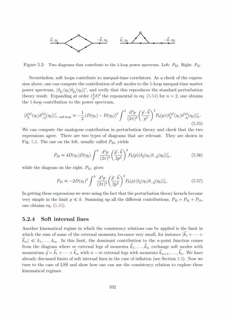
~k1, 1
~k1, 1~k2, 2
~k2, 2
~q1, 1 ~q1, 1
~q2, 2 ~q2, 2
~q1 ~q1
~q2~q2
~k1
~k1 + ~q1
~k2 + ~q2
~k1 ~q1
~k, 1 ~k, 2 ~k, 1 ~k, 2
Thursday, October 31, 13
Figure 5.2: Two diagrams that contribute to the 1-loop power spectrum. Left: P22. Right: P31.
Nevertheless, soft loops contribute to unequal-time correlators. As a check of the expres-
sion above, one can compute the contribution of soft modes to the 1-loop unequal-time matter
power spectrum, 〈δ~k1(η1)δ~k2
(η2)〉′, and verify that this reproduces the standard perturbation
theory result. Expanding at order (kpδ)2 the exponential in eq. (5.54) for n = 2, one obtains
the 1-loop contribution to the power spectrum,
〈δ(g)~k
(η1)δ(g)
−~k(η2)〉′1−soft loop ≈ −
1
2(D(η1)−D(η2))2
∫ Λ d3p
(2π)3
(~p · ~kp2
)2
P0(p)〈δ(g)~k
(η1)δ(g)
−~k(η2)〉′0 .
(5.55)
We can compute the analogous contribution in perturbation theory and check that the two
expressions agree. There are two types of diagrams that are relevant. They are shown in
Fig. 5.2. The one on the left, usually called P22, yields
P22 ≈ 4D(η1)D(η2)
∫ Λ d3p
(2π)3
(~p · ~k2p2
)2
P0(p)〈δ~k(η1)δ−~k(η2)〉′0 , (5.56)
while the diagram on the right, P31, gives
P31 ≈ −2D(η1)2
∫ Λ d3p
(2π)3
(~p · ~k2p2
)2
P0(p)〈δ~k(η1)δ−~k(η2)〉′0 . (5.57)
In getting these expressions we were using the fact that the perturbation theory kernels become
very simple in the limit p k. Summing up all the different contributions, P22 + P31 + P13,
one obtains eq. (5.55).
5.2.4 Soft internal lines
Another kinematical regime in which the consistency relations can be applied is the limit in
which the sum of some of the external momenta becomes very small, for instance |~k1 + · · ·+~km| k1, . . . , km. In this limit, the dominant contribution to the n-point function comes
from the diagram where m external legs of momenta ~k1, . . . , ~km exchange soft modes with
momentum ~q = ~k1 + · · ·+~km with n−m external legs with momenta ~km+1, . . . , ~kn. We have
already discussed limits of soft internal lines in the case of inflation (see Section 4.3). Now we
turn to the case of LSS and show how one can use the consistency relation to explore these
kinematical regimes.
102
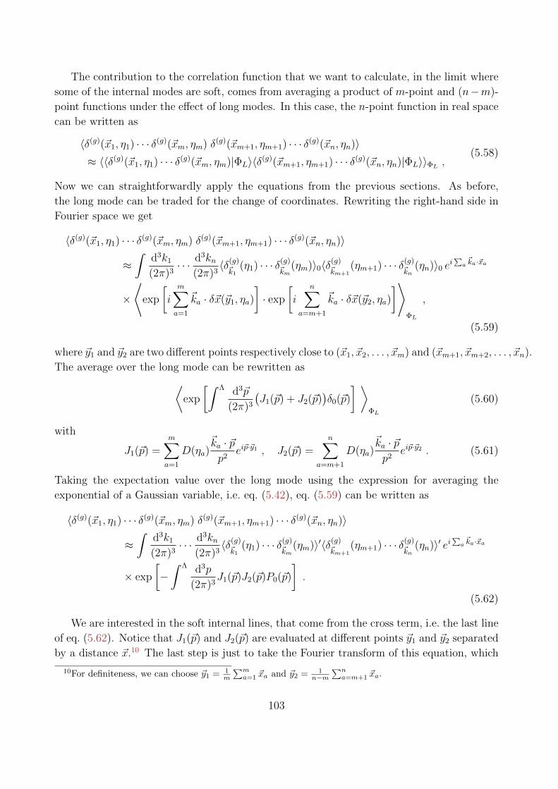
The contribution to the correlation function that we want to calculate, in the limit where
some of the internal modes are soft, comes from averaging a product of m-point and (n−m)-
point functions under the effect of long modes. In this case, the n-point function in real space
can be written as
〈δ(g)(~x1, η1) · · · δ(g)(~xm, ηm) δ(g)(~xm+1, ηm+1) · · · δ(g)(~xn, ηn)〉≈ 〈〈δ(g)(~x1, η1) · · · δ(g)(~xm, ηm)|ΦL〉〈δ(g)(~xm+1, ηm+1) · · · δ(g)(~xn, ηn)|ΦL〉〉ΦL ,
(5.58)
Now we can straightforwardly apply the equations from the previous sections. As before,
the long mode can be traded for the change of coordinates. Rewriting the right-hand side in
Fourier space we get
〈δ(g)(~x1, η1) · · · δ(g)(~xm, ηm) δ(g)(~xm+1, ηm+1) · · · δ(g)(~xn, ηn)〉
≈∫
d3k1
(2π)3· · · d3kn
(2π)3〈δ(g)~k1
(η1) · · · δ(g)~km
(ηm)〉0〈δ(g)~km+1
(ηm+1) · · · δ(g)~kn
(ηn)〉0 ei∑a~ka·~xa
×⟨
exp
[im∑a=1
~ka · δ~x(~y1, ηa)
]· exp
[i
n∑a=m+1
~ka · δ~x(~y2, ηa)
]⟩ΦL
,
(5.59)
where ~y1 and ~y2 are two different points respectively close to (~x1, ~x2, . . . , ~xm) and (~xm+1, ~xm+2, . . . , ~xn).
The average over the long mode can be rewritten as⟨exp
[∫ Λ d3~p
(2π)3
(J1(~p) + J2(~p)
)δ0(~p)
] ⟩ΦL
(5.60)
with
J1(~p) =m∑a=1
D(ηa)~ka · ~pp2
ei~p·~y1 , J2(~p) =n∑
a=m+1
D(ηa)~ka · ~pp2
ei~p·~y2 . (5.61)
Taking the expectation value over the long mode using the expression for averaging the
exponential of a Gaussian variable, i.e. eq. (5.42), eq. (5.59) can be written as
〈δ(g)(~x1, η1) · · · δ(g)(~xm, ηm) δ(g)(~xm+1, ηm+1) · · · δ(g)(~xn, ηn)〉
≈∫
d3k1
(2π)3· · · d3kn
(2π)3〈δ(g)~k1
(η1) · · · δ(g)~km
(ηm)〉′〈δ(g)~km+1
(ηm+1) · · · δ(g)~kn
(ηn)〉′ ei∑a~ka·~xa
× exp
[−∫ Λ d3p
(2π)3J1(~p)J2(~p)P0(~p)
].
(5.62)
We are interested in the soft internal lines, that come from the cross term, i.e. the last line
of eq. (5.62). Notice that J1(~p) and J2(~p) are evaluated at different points ~y1 and ~y2 separated
by a distance ~x.10 The last step is just to take the Fourier transform of this equation, which
10For definiteness, we can choose ~y1 = 1m
∑ma=1 ~xa and ~y2 = 1
n−m
∑na=m+1 ~xa.
103
gives
〈δ(g)~k1
(η1) · · · δ(g)~km
(ηm)δ(g)~km+1
(ηm+1) · · · δ(g)~kn
(ηn)〉′
≈ 〈δ(g)~k1
(η1) · · · δ(g)~km
(ηm)〉′ 〈δ(g)~km+1
(ηm+1) · · · δ(g)~kn
(ηn)〉′
×∫
d3x e−i∑mi=1
~ki·~x exp
[−∫ Λ d3p
(2π)3ei~p·~x
m∑a=1
D(ηa)~ka · ~pp2
n∑a=m+1
D(ηa)~ka · ~pp2
P0(p)
].
(5.63)
The last line encodes the effect of soft modes with total momentum ~q = ~k1 + · · · + ~kmexchanged between m external legs of momenta ~k1, . . . , ~km and n − m external legs with
momenta ~km+1, . . . , ~kn, in the limit q/ki → 0. Expanding the exponential at a given order in
P0(p) counts the number of soft lines exchanged. The integral in d3x ensures that the sum of
the internal momenta is ~q.
As a concrete example, let us consider the case m = 2, n = 4, i.e. a 4-point function in
the collapsed limit |~k1 + ~k2| k1, k2, and the exchange of a single soft line. In this case,
expanding the exponential at first order in P0(p), the equation above gives
〈δ~k1(η1)δ~k2
(η2)δ~k3(η3)δ~k4
(η4)〉′c≈ −〈δ(~k1, η1)δ(~k2, η2)〉′〈δ(~k3, η3) · · · δ(~k4, η4)〉′
×∫ Λ
d3p(D(η1)−D(η2)
)~k1 · ~pp2
(D(η3)−D(η4)
)~k3 · ~pp2
P0(p)δD(~p− ~k1 − ~k2) ,
(5.64)
where we have considered only the connected diagram and, for simplicity, we are neglecting
soft loops attached to each lines. To compare with perturbation theory, we need to compute
the tree-level exchange diagram. This can be easily done in the limit when the exchanged
momentum is small. The contribution from taking ~k1 and ~k3 at second order is
T2121 ≈ −4D(η1)D(η3)P0(|~k1+~k2|)~k1 · (~k1 + ~k2)
2|~k1 + ~k2|2~k3 · (~k1 + ~k2)
2|~k1 + ~k2|2〈δ~k1
(η1)δ~k2(η2)〉′〈δ~k3
(η3)δ~k4(η4)〉′ .
(5.65)
If we include the other permutations we finally get
〈δ~k1(η1)δ~k2
(η2)δ~k3(η3)δ~k4
(η4)〉′c ≈ −(D(η1)−D(η2)
)(D(η3)−D(η4)
)P0(|~k1 + ~k2|)
×~k1 · (~k1 + ~k2)
|~k1 + ~k2|2~k3 · (~k1 + ~k2)
|~k1 + ~k2|2〈δ~k1
(η1)δ~k2(η2)〉′〈δ~k3
(η3)δ~k4(η4)〉′ ,
(5.66)
which is indeed the same as eq. (5.64).
5.3 Consistency Relations in Redshift Space
So far we were considering consistency relations in real space (and corresponding momentum
space). As we saw, one of their main virtues is that they hold non-perturbatively, even when
104

baryonic physics is taken into account. For this reason they should hold directly at the level
of the correlation functions of galaxy overdensities and checking if they hold in real data can
help us to test the assumptions that enter in the derivation of the consistency relations.
However, galaxy surveys do not tell us about positions of galaxies in real space, but in
redshift space. If one does not want to restrict only to large scales, the mapping between the
two is very non-trivial and depends on the dynamics of the modes (in particular velocities)
even in the non-perturbative regime. It is therefore impossible to exploit the full potential of
the consistency relations at the level of observables, unless they can be rewritten in redshift
space without using any approximations.
This is not a trivial task. One approach would be to start form the consistency relations
in real space and try to rewrite them in redshift space. As we said, for this approach to work,
one has to know the exact velocities of all particles, needed for the mapping between real
and redshift space. Of course, this is impossible. One may hope that even without solving
for the velocities, the effects of mapping will still somehow “resum” on both sides of the
consistency relation, leading to a simple result. But even in the simplest case, if we use the
fluid approximation11, any n-point correlation function in real space is an infinite sum of all
correlation functions in redshift space of order higher than n. This makes the task of going
from real to redshift space very difficult to complete.
Luckily, there is a simple trick to derive the consistency relations directly in redshift space,
without using the real space result as a starting point. In the following Section we present
this derivation [69, 71].
5.3.1 Derivation
For simplicity, let us work in the plane-parallel approximation12. The mapping between real
space ~x and redshift space ~s is given by
~s = ~x+vzH z , (5.67)
where z is the direction of the line of sight, vz ≡ ~v · z, and ~v is the peculiar velocity of a
given object. The relation between z and η also receives corrections due to peculiar velocities.
However, these corrections are small for sufficiently distant objects for which v Hx. Notice
that we do not assume that the peculiar velocity is a function of the position ~x since this
holds only in the single-stream approximation, which breaks down for virialized objects on
small scales [146, 147].
With this setup, the derivation of the consistency relations in redshift space follows closely
what we did in real space. Intuitively, the long mode has two important effects. It again
11In this case the system is fully described by density and velocity fields. Every point in space has only one
velocity vector and the mapping between real and redshift space in “one-to-one”. This is not the case when
the fluid approximation breaks down.12This approximation is valid on small angular scales only. For a large fraction of the sky, one has to rederive
the consistency relations in terms of appropriate observables, which is beyond the scope of this thesis.
105

induces a time-dependent translation of real coordinates that we discussed so far. However,
in redshift space one has to take into account the effects on velocities. Given that the long
mode makes all objects moving with the same bulk velocity, there is an additional translation
in redshift space, and this will lead to an additional term in the consistency relation. Let us
see how this intuition can be made more formal.
The effect of the long mode on coordinates and velocities is
~x→ ~x+D ~∇Φ0,L , (5.68)
~v → ~v + fHD ~∇Φ0,L . (5.69)
As we already saw, in these equations D(η) is the growth factor, f(η) ≡ d lnD/d ln a is the
growth rate and ~∇Φ0,L a homogenous gradient of the initial gravitational potential Φ0,L. Now
we can use eq. (5.67) to find a corresponding translation in redshift space
~s = ~s+D(η) · (~∇Φ0,L + f∇zΦ0,Lz) . (5.70)
The first term is just a familiar translation in real space, while the second one captures the
effects of the bulk velocity induced by the long mode.
Now the derivation of the consistency relation is straightforward. As in real space, we
can start from the fact that the same redshift-space correlation functions in the presence or
the absence of a long mode ΦL are related only by a translation (5.70) in redshift space.
Therefore, we can write
〈δ(g)s (~s1, η1) · · · δ(g)
s (~sn, ηn)|ΦL〉 ≈ 〈δ(g)s (~s1, η1) · · · δ(g)
s (~sn, ηn)〉=∑a
δ~sa〈δ(g)s (~s1, η1) · · · ~∇aδ
(g)s (~sa, ηa) · · · δ(g)
s (~sn, ηn)〉 , (5.71)
where δ~sa ≡ D(ηa) (~∇aΦ0,L + fa∇a,zΦ0,Lz). This statement is non-trivial because it involves
a statistical average. To show that it is correct in a more rigorous way, we can notice that
the density in redshift space can be written in terms of the real-space distribution function
in the following way [146, 147]
ρs(~s) = ma−3
∫d3p f
(~s− vzH z, ~p
). (5.72)
In this equation m is the mass of the particles and ~p is the physical momentum. In the
presence of the long mode, the distribution function ρs(~s) can be written as
ρs(~s)ΦL =m
a3
∫d3p f
(~s− vzH z + δ~x, ~p+ amδ~v
)=m
a3
∫d3p′ f
(~s− vz − δvz
H z + δ~x, ~p′)
= ρs(~s+ δ~s), (5.73)
where δx and δ~v are given by eqs. (5.68) and (5.69).
106

At this point what remains to be done is just to go to the Fourier space conjugate to
redshift space coordiantes. It is straightforward to see that eq. (5.71) becomes
〈Φ0(~q)δ(g)s ~k1
(η1) · · · δ(g)s ~kn
(ηn)〉′
≈ PΦ(q)∑a
D(ηa)[~q · ~ka + f(ηa)qz ka,z
]〈δ(g)s ~k1
(η1) · · · δ(g)s ~kn
(ηn)〉′ . (5.74)
The most difficult task of dealing with the short modes is done in this way. If we want to write
everything in terms of observables in redshift space, the last step is to express the long mode
gravitational potential as a function of the density contrast δ(g)s . This is not very difficult,
since the long mode is in the linear regime. Assuming that a simple linear bias model works
well on large scales we can write
δ(g)s (~q, η) = −(b1 + fµ2
~q)D(η)q2Φ0(~q) , (5.75)
where b1 is a linear bias parameter between galaxies and dark matter and µ~k ≡ ~k · z/k. With
this approximations the consistency relation above takes its final form
〈δ(g)s ~q(η)δ(g)
s ~k1(η1) · · · δ(g)
s ~kn(ηn)〉′ ≈− Pg,s(q, η)
b1 + fµ2~q
∑a
D(ηa)
D(η)
kaq
[q · ka + f(ηa)µ~q µ~ka
]× 〈δ(g)
s ~k1(η1) · · · δ(g)
s ~kn(ηn)〉′ .
(5.76)
As we expected, the only important difference compared to the real space result is the addi-
tional term related to the bulk velocity.
Everything we said so far about the non-relativistic consistency relation in real space
holds also in redshift space. It is a non-perturbative statements that is exact even when
the baryonic physics is taken into account. The expression above is non-perturbative inkqδL, and all results involving multiple soft limits, loops, internal soft legs and others can be
straightforwardly generalized to redshift space.
One of the properties of the consistency relation in real space was that it vanishes (up to
sub-leading corrections in q) for equal-time correlation functions. As we stressed, this can be
used as a tool to look for deviations from the consistency relation and test the assumptions
that enter its derivation. It is important to stress that the same thing holds even in redshift
space. This is not surprising because, after all, the long mode is still just a translation that
has slightly different form than before. Given that it does not change the distances between
the points in redshift space and that everything is translationally invariant, the variation of
the equal-time correlation functions is just zero. This observation is crucial for the tests of
the Equivalence Principle that we are going to discuss in the following Section. Before that,
let us do a small check of the equation (5.76).
5.3.2 Checks
As we did so far, we can check the consistency relations of LSS in redshift space using the
correlation functions calculated in perturbation theory. Let us start with the three-point
107

function. The redshift space bispectrum is given by [101]
〈δ(g)s ~q(η)δ(g)
s ~k1(η1)δ(g)
s ~k2(η2)〉′ =
2Z2(−~q,−~k2; η1)Z1(~q; η)Z1(~k2; η2)〈δ(~q, η)δ(−~q, η1)〉′〈δ(~k1, η1)δ(~k2, η2)〉′ + cyclic ,(5.77)
where
Z1(~k; η) ≡ (b1 + fµ2~k) ,
Z2(~ka, ~kb; η) ≡ b1F2(~ka, ~kb) + fµ2~kG2(~ka, ~kb)
+fµ~kk
2
[µ~kaka
(b1 + fµ2~kb
) +µ~kbkb
(b1 + fµ2~ka
)
]+b2
2.
(5.78)
In these formulas b1 and b2 are the linear and non-linear bias parameters and F2 and G2 are
the standard second-order perturbation kernels for density and velocity respectively [101]. In
the limit q → 0 the kernels simplify in the following way
2Z2(−~q,−~k2; η1) ≈ (b1 + f1µ2~k2
)~q · ~k2
q2+ (b1 + f1µ
2~k2
)f1k2
qµ~qµ~k2
. (5.79)
Using this result we can rewrite the redshift space three-point function in the squeezed limit
in the following way
〈δ(g)s ~q(η)δ(g)
s ~k1(η1)δ(g)
s ~k2(η2)〉′
≈ Pg,s(q, η)
b1 + fµ2~q
D(η1)
D(η)(b1 + f1µ
2~k2
)
(~q · ~k2
q2+ f1
k2
qµ~qµ~k2
)Z1(~k2; η2)〈δ(~k1, η1)δ(~k2, η2)〉′
≈ −Pg,s(q, η)
b1 + fµ2~q
D(η1)
D(η)
k1
q(q · k1 + f1µ~qµ~k1
)〈δ(~k1, η1)δ(~k2, η2)〉′ + (1↔ 2) .
(5.80)
Notice that this is exactly the right hand side of the eq. (5.76) in the case n = 2. Therefore,
we can conclude that the consistency relation is satisfied.
5.4 Violation of the Equivalence Principle
In previous sections we showed that one can derive a fully relativistic consistency relation
of LSS, showed how it simplifies in the non-relativistic regime and proved that the relation
remains almost unchanged when written in terms of observables in redshift space. For the
case of equal-time (or equal-redshift) correlation functions, the consistency relation seems
somewhat trivial13
limq→0〈δ~q(η)δ~k1
(η)δ~k2(η)〉′ = O
[(q/k)0
]. (5.81)
13For the rest of this section we will focus only on the three-point function which is observationally the
most relevant. We are also going to work with the real space expressions because they are simpler and the
additional terms in the redshift space equations do not change any of the conclusions.
108

As we saw, the fact that the squeezed limit of the (n+ 1)-point function vanishes at leading
order in q is just a consequence of the translational invariance. The effect of the long mode
is just to induce some bulk velocity and “translate” the short modes. Given the translational
invariance, the variation of the n-point function on the right hand side is simply zero.
As we pointed out at the beginning of this Chapter, there are two important assumptions
in this line of reasoning. The first one is that there is no statistical correlation between the
long and short modes in the initial conditions. In other words we have to assume that local
non-Gaussianities are very small. This happens in all single-field models of inflation, as we
already discussed in the previous Chapter. The second assumption is that the long mode
affects all objects in the same way. In other words we have to assume that the EP holds on
cosmological scales.
Any violation of any of these two assumptions would lead to a violation of the consistency
relation. For example, it is well-known that in the presence of the local non-Gaussianities the
squeezed limit of the three-point function is given by (see for example [148])
limq→0〈δ~q(η)δ~k1
(η)δ~k2(η)〉′ ≈ 6f locNL
Ωm,0H20
q2T (q)P (q, η)P (k, η) . (5.82)
This is a consequence of the fact that although dynamically it does not do anything, the long
mode affects the statistics of the initial conditions for the short modes. As a consequence, this
changes the evolution on the short scales and the correlation “survives” until late times. The
other way to see the same effect is through the so-called scale-dependent bias. There is a lot
of observational effort to use the scale-dependence of the bias or divergences in the squeezed
limit of the three-point function to constrain the amplitude of the local non-Gaussianities
f locNL. Our best current constraints that come from LSS use these techniques.
In this Section we will focus on the other possible source of violation of the consistency
relation — a violation of the EP on cosmological scales [70, 71, 68]. If the EP is violated, then
the effect of the long mode even on equal-time correlation functions is not trivial. Different
objects will fall in a different way in the homogeneous gravitational field induced by the long
mode. The long mode is not just a change of coordinates anymore and although there is no
way to calculate its effect non-perturbatively, one can claim that in general in the squeezed
limit we expect
limq→0〈δ~q(η)δ
(A)~k1
(η)δ(B)~k2
(η)〉′ =(ε~k · ~qq2
+O[(q/k)0
])P (q, η)PAB(k, η) , (5.83)
where A and B are two different kind of objects that behave in a different way in the presence
of a gravitational field induced by the long mode δ~q. We can see that in the absence of the
EP ε is different form zero and the squeezed limit of the equal-time three-point function has
a divergence that goes like k/q. Therefore, assuming single-field inflation, any detection of a
divergence in the squeezed limit of the three-point function would be a signal for a violation
of the EP.
Notice that the equations (5.82) and (5.83) have a very similar form. Apart form constants
and different scaling with momenta, they are both divergent in q → 0 limit. As we are going
109

to see, this means that we can use the same method for forecasting how well we can constrain
f loc.NL to constrain the violation of the EP on cosmological scales. The parameter that plays the
role of f loc.NL in this case is ε. However, we have to stress that there is one important difference
between (5.82) and (5.83). While for constraining the local non-Gaussianities one can use the
standard power spectra and bispectrum, in the case of a violation of the EP it is crucial to
cross-correlate two objects of different kinds A and B. Therefore, for making the constraints
tighter, is is crucial to be able to separate different kind of objects in galaxy surveys or other
observations. We will come back to this issue later.
In the rest of this Section we are going to explore in more detail how well we can constrain
the EP using the consistency relations. Before moving on, let us stress here that the statement
we made holds directly on the level of observables — galaxy number densities in redshift
space. This is the main advantage of using the consistency relations. Moreover, looking for a
violation of the consistency relation, we do a model independent test of GR on cosmological
scales because we do not have to assume any model of modified gravity. The only choice we
have to make is what classes of objects A and B we want to cross-correlate.
5.4.1 Modifications of gravity and EP violation
Equation (5.83) is a general result that does not depend on the underlying modification of
GR. In GR (and assuming single-field inflation) the right hand side vanishes. Therefore, if the
EP is violated on cosmological scales, whatever is the mechanism, the squeezed limit of the
three-point function must be given by eq. (5.83). In principle, this is enough to proceed and
estimate how well we can constrain violations of the EP using LSS. However, in this section,
we would like to give a very brief overview of some of the most popular modifications of GR
that can induce violations of the EP on cosmological scales (for a review, see for example
[149]). The list is certainly not complete, but we need it just to give a flavour of what kind
of effects one can expect.
The main motivation for looking for modifications of GR is the accelerated expansion
of the universe. The value of cosmological constant needed to explain the acceleration is
unnaturally small, and it is interesting to explore whether it is possible to consistently modify
GR such that gravity behaves differently on cosmological scales, while keeping the standard
form on small scales where we have a lot of experimental evidence that GR works just fine.
Over the years, several models of consistent infrared modifications of GR were proposed. All
of them have the common property that they pass Solar System tests (typically the effects
of modifying GR are unobservable due to some “screening” mechanism) and make significant
modification only on the cosmological scales. Based on the screening mechanism there are
several models and we will discuss some of them. We are also going to mention other possible
sources of the EP violation.
For all of these possibilities there are already good constraints coming from precise mea-
surements in Solar System and the study of structure formation. As we are going to see,
some of them are stronger than what we can get using the consistency relation violations.
110
However, it is important to stress that constraints coming from the squeezed limit of the
three-point function are model independent (up to the choice of objects to cross correlate). If
the accelerated expansion of the universe really has to do with modifications of GR on large
scales, it can still be that our current theories are the final word on the subject and any model
independent tests are worth doing.
Let us now go through some of the situations in which the EP is violated.
Screening. The screening of extra forces needed to satisfy the Solar System constraints
induces violations of the EP [150]. Depending on the screening mechanism, there are several
relevant cases. We focus on some of them.
One possibility is chameleon [151] or symmetron [152, 153, 154] screening. The screening
in these models depends on the typical value of the gravitational potential GM/r of the
object and the EP violation can be of order unity between screened and unscreened objects.
However, imposing the screening inside the Solar System makes the impact of the fifth force
on cosmological scales very limited. One can show that there is a model-independent limit
on the mass of the scalar [155, 156]
m2 & 106α2H2 , (5.84)
where α2 measures a deviation from GR. This inequality is valid at low redshifts and limits
the effect of the scalar on short scales k/a . m. We will show later how this bound compares
with the constraints one can get form a violation of the consistency relations.
The other possibility is Galileon screening [135]. In this case, due to the nonlinearities of
the scalar equations, the issue of the EP violation is quite subtle. On one hand, one can show
that an object immersed in an external field which is constant over the size of the object will
receive an acceleration proportional to the mass and independent of the possible Vainshtein
screening of the object [150]. On the other hand, due to the nonlinearities, the value of the
external field may not be the same before and after the object is put into place. For example,
the Moon changes the solution of the Galileon around the Earth and the nonlinearity of the
system is such that the acceleration the Moon experiences is different from the one of a test
particle orbiting around the Earth [157, 158].
The complicated nonlinear behaviour in the Galileon screening and related violations of
the EP are hard to control in general. This is why it is a bit surprising that one can actually
prove that the Galileon models do not induce violations of the consistency relations. To see
this let us focus on the non-relativistic limit of structure formation. Deep inside the horizon,
structure formation in the presence of the Galileon π is governed by the following equations
~v + (~v · ~∇)~v = −~∇Φ− α~∇π , (5.85)
F (∂i∂jπ) = α8πGρ , (5.86)
∇2Φ = 4πGρ , (5.87)
where F is the equation of motion for the Galileon, which only depends on the second deriva-
tives of π. The point is that one can apply the same argument as in the standard case. A long
111
mode of Φ+απ, up to first order in gradients, can be removed just by a change of coordinates.
As before, this change of coordinates brings us to an accelerated frame. For this to happen
the symmetry of Galileons is crucial, since it makes a homogeneous gradient of π drop out
of eq. (5.86) [159]. However, it is important to notice that this works only deep inside the
horizon. Only in the non-relativistic regime, when time-derivatives can be neglected, we can
remove a homogeneous field with arbitrary time-dependence although this is not a symmetry
of the full Galileon theory. This does not happen, for example, in the case of the chameleon
and there we expect the consistency relation to be violated.
One important step in the argument above is to make sure that the long mode induced by
a change of coordinates is a physical mode. This is indeed the case. The homogenous gradient
can describe a long mode in the linear regime as shown in simulations [160, 161, 162, 163, 164].
This means that, assuming no primordial local non-Gaussianity, the effect of a long mode boils
down to the change of coordinates. This is a time dependent translation which does not give
any effect for equal-time correlation functions.
Another example of the screening mechanism is K-mouflage [165], where the screening
depends on the first derivative of the gravitational potential. This happens in theories with
a generic kinetic term of the form P (X) with X ≡ (∂φ)2. Although this case has not been
thoroughly studied, there is no reason to expect that the consistency relations holds. In the
absence of Galileon symmetry in the non-relativistic limit, the argument above does not go
through.
Baryon content. If dark matter and baryons have a different coupling with a light scalar,
one has a violation of the EP at the fundamental level. This causes different astrophysical
objects, with a different baryon/dark matter ratio to fall at different rates in an external field.
This scenario is however very constrained: Planck [166] limits this kind of couplings to be
. 10−4 smaller than gravity. This is far from what we can achieve with our method, since most
astrophysical objects have a quite similar baryon content and this suppresses substantially
the EP violation.
Gravitational potential. The no-hair theorem implies that black-holes do not couple with
a scalar force. More generally, the mass due to self-gravity will violate the EP in the presence
of a fifth force. Unfortunately, it seems impossible to observe isolated objects with a sizable
component of gravitational mass. The mass of clusters only receives a contribution in the
range 10−5 ÷ 10−4 from the gravitational potential and the correction is even smaller for less
massive objects. Black holes, whose mass is entirely gravitational in origin, do not significantly
contribute to the mass of the host galaxy.
Environment. Another possibility is to divide the objects depending not on some intrinsic
feature but on their environment, for example comparing galaxies in a generic place against
galaxies in voids [71]. The fifth force tends to be screened in a dense environment (blanket
screening), while it is active in voids. Notice that this is not a test of the Galilean EP (different
112

objects fall at the same rate in the same external field), but it still checks whether the effect
of the long mode can be reabsorbed completely by a change of coordinates. The arguments
made above for the Galileon case work also here and we expect no violation of the consistency
relation in this case. This effect will be present in the case of chameleon screening (with the
same limitations on the Compton wavelength discussed above) and in K-mouflage.
In all these examples, as a consequence of a EP violation, there are different kinds of
astrophysical objects (or they are in a different environment) that behave in different ways
in an external gravitational field induced by the long mode. We can describe this generic
situation using a toy model in which the universe is composed of two non-relativistic fluids A
and B, with the latter coupled to a scalar field mediating a fifth force. For example, the two
fluids could be baryons and dark matter, but the model can also describe two populations of
astrophysical objects, like two different types of galaxies. If the scalar field ϕ has a negligible
time evolution, the continuity equations of the two fluids are the same,
δ′X + ~∇ · [(1 + δX)~vX ] = 0 , X = A,B , (5.88)
where a prime denotes the derivative with respect to the conformal time η, ′ ≡ ∂η. The Euler
equation of B contains the fifth force, whose coupling is parameterized by α,
~v′A +H~vA + (~vA · ~∇)~vA = −~∇Φ , (5.89)
~v′B +H~vB + (~vB · ~∇)~vB = −~∇Φ− α~∇ϕ , (5.90)
where H ≡ ∂ηa/a is the comoving Hubble parameter. To close this system of equations we
need Poisson’s equation and the evolution equation of the scalar field. Assuming that the
scalar field stress-energy tensor is negligible, only matter appears as a source in Poisson’s
equation,
∇2Φ = 4πGρm δ = 4πGρm (wAδA + wBδB) , (5.91)
where ρm is the total matter density and wX ≡ ρX/ρm is the density fraction of the X species.
Moreover, in the non-relativistic approximation we can neglect time derivatives in comparison
with spatial gradients and the equation for the scalar field reads
∇2ϕ = α · 8πGρmwBδB , (5.92)
where we have neglected the mass of the scalar field, assuming we are on scales much shorter
than its Compton wavelength.
Using this setup one can proceed and using perturbation theory calculate explicitly the
three-point functions of density perturbations. We leave the details of the calculation for
Appendix C. The most interesting three-point function in the squeezed limit is given by
limq→0〈δ~q(η)δ
(A)~k1
(η)δ(B)~k2
(η)〉′ ' 7
5wB α
2~k · ~qq2
P (q, η)PAB(k, η) . (5.93)
As we expect, the result is proportional to k/q and it has the form of eq. (5.83).
113

The result that we obtained remains qualitatively the same if A or B represent extended
objects, for example a fluid of galaxies of a given kind [167]. For instance, one can take A
to represent galaxies that are not coupled to the fifth force because they are screened (see
Sec. 5.4.1), while B represents the dark matter fluid. In this case one should start from initial
conditions in which there is a bias between the galaxy and the dark matter overdensities:
ua = (bg, 1, b, b) (for the definition see Appendix C). This is equivalent to exciting decaying
modes, given that asymptotically the galaxy bias becomes unity14 (bg is the initial galaxy
bias). Consequently, the result (5.93) will be different. Still, it is straightforward to check
that, as expected, there is no 1/q divergence if the EP is not violated, i.e. α = 0. In the limit
wA 1 (i.e. the screened galaxies contribute a subdominant component of the overall mass
density) and keeping only the slowest decaying mode, one gets (in this case we take the long
mode to be dark matter only)
limq→0〈δ(B)~q (η)δ
(A)~k1
(η)δ(B)~k2
(η)〉′ ' 7
5α2~k · ~qq2
(1 +
10
7(bg − 1)e−(y−y0)
)P (q, η)PAB(k, η) . (5.94)
Where y is the logarithm of the linear growth factor, y ≡ lnD+ (see Appendix C). Notice
that y0 here represents the initial value when the local galaxy bias bg is set up.
Of course, this model is quite rough to capture all processes in a realistic process of
structure formation. For example, one possible complication comes from the fact that objects
become screened only at a certain stage of their evolution, so that the coupling of the fluid A
with the scalar is time-dependent. However, this and other subtleties cannot change the form
of the final result, but just modify the numerical value on the right-hand side of eq. (5.93) by
a factor of order one. In any case, given the model-dependence of the result, in the following
Section where we estimate the possible constraints on the EP violation, we will stick to
eq. (5.93) as our benchmark model.
5.4.2 Signal to noise for the bispectrum
Let us finally focus on the question how well we can constrain the violation of the EP using
large scale structure surveys. In order to address this question quantitatively, we have to
calculate the signal to noise ratio for a given model that violates the EP. We will use our
toy model described in the previous Section, but the constraints can be straightforwardly
translated to other models of modified gravity. Given that equations (5.82) and (5.83) are
quite similar, the calculation closely follows the standard approach used to make forecasts for
constraining the primordial non-Gaussianities (see for example [168]).
Before moving to a more detailed calculation, we can try to roughly estimate what kind of
constraints we can get just counting the number of modes available in the survey. The simple
way to do it is as follows. The experimental constraint on f locNL goes like ∆f loc
NL ∼ 5√
106/N ,
where N is the number of available modes in the survey. This is consistent with the Planck
limit f locNL . 5, for N ∼ 106 [13]. If we turn to the large scale structure and consider a survey
14Here we are assuming conservation of galaxies.
114
with a volume V ∼ 1(h−1Gpc)3 and kmax of the order of the non-linear scale, then the number
of modes is N ∼ (kmax/kmin)3 ∼ 4 · 103 and so ∆f locNL ∼ 80. This is in a good agreement with
Fig. 3 of Ref. [168]. To get the constraints on the EP violation we only have to compare the
equations (5.82) and (5.83) and see that f locNL ∼ α2 × q k/(ΩmH
20 ). Assuming k/q ∼ 10, a
bound on α2 is of the order 10−3.
To make this estimate more precise, we will do the full signal-to-noise calculation. Let
us imagine that we have a survey of a given comoving volume V . This volume defines the
fundamental scale in momentum space, kf = 2π/V 1/3. This means that we cannot measure
the modes with momentum smaller than kf . In this setup, the bispectrum estimator is given
by
B(k1, k2, k3) =VfV123
∫k1
d3~q1
∫k2
d3~q2
∫k3
d3~q3 δ(~q1 + ~q2 + ~q3) · δ~q1δ~q2δ~q3 , (5.95)
where Vf = (2π)3/V is the volume of the fundamental cell and the integration is done over
the spherical shells with bins qi ∈ (ki − δk/2, ki + δk/2). The volume V123 is given by
V123 ≡∫k1
d3~q1
∫k2
d3~q2
∫k3
d3~q3 δ(~q1 + ~q2 + ~q3) ≈ 8π2 k1k2k3 δk3 . (5.96)
In what follows we will assume no significant correlation among different triangular configura-
tions. In other words, we assume that the bispectrum covariance matrix is diagonal and given
by a Gaussian statistics. This is a good approximation for the modes in the linear regime
that we are interested in. Under this assumption the variance is given by
∆B2(k1, k2, k3) = k3f
s123
V123
Ptot(k1)Ptot(k2)Ptot(k3) , (5.97)
where s123 = 6, 2, 1 for equilateral, isosceles and general triangles, respectively. The power
spectrum Ptot(k) contains two parts
Ptot(k) = P (k) +1
(2π)3
1
n. (5.98)
The first term is the standard power spectrum, while the second accounts for the shot noise.
For example, in a galaxy survey, n is the number density of galaxies. In what follows we
will neglect the shot noise contribution. The first reason is that for our estimates we use
only modes that are in the linear regime where the shot noise is expected to be negligible.
Furthermore, neglecting the shot noise we can estimate the total amount of signal in principle
available for a survey of a given volume. In this way we do not restrict our analysis specifically
to galaxy surveys.
Given the definitions above, the signal-to-noise ratio is calculated as(S
N
)2
=∑T
(Bnew physics(k1, k2, k3)−Bstandard(k1, k2, k3))2
∆B2(k1, k2, k3), (5.99)
where the sum runs over all possible triangles formed by ~k1, ~k2 and ~k3 given kmin and kmax. It
is possible to write the sum in such a way that the same triangles are not counted twice. The
115

symmetry factor s123 is then used to take into account some special configurations. In the
case with two different species of particles that we study in our toy model, the bispectrum
is not symmetric when momenta are exchanged and the sum in the signal-to-noise has to be
written accordingly. The simplest way is to impose s123 = 1 for all configurations and the
sum over triangles in the following way
∑T
≡kmax∑
k1=kmin
kmax∑k2=kmin
k∗max∑k3=k∗min
, (5.100)
where k∗min ≡ max(kmin, |~k1 − ~k2|), k∗max ≡ min(|~k1 + ~k2|, kmax) and the discrete sum is done
with |~kmax − ~kmin|/δk steps where we set δk to be the same as the fundamental scale kf .
Let us now apply this machinery to the toy model with two fluids we discussed at the end
of the previous Section. We expect that the signal-to-noise will get the largest contribution
from the squeezed configurations. However, to be completely general, we will keep the full
result for the bispectrum (calculated up to first order in α2) in the analysis. The details of
the calculation can be found in Appendix C. For the toy model, the signal-to-noise is given
by (S
N
)2
=∑T
[B
(AB)
α2 (k1, k2, k3)−B(AB)
α2=0(k1, k2, k3)]2
∆[B(AB)]2(k1, k2, k3), (5.101)
where the bispectrum B(AB)(k1, k2, k3) is defined by
〈δ~k1(η)δ
(A)~k2
(η)δ(B)~k3
(η)〉 = (2π)3δD(~k1 + ~k2 + ~k3)B(AB)(k1, k2, k3) , (5.102)
and the left hand side of this equation is computed at leading order in α2. In order to do the
calculation we use
δ(A)(k) ≡ 1
wA + wBbδ(k) , δ(B)(k) ≡ 1
wA/b+ wBδ(k) , (5.103)
where the transfer function of the total matter density contrast δ is computed with CAMB
[169]. With the following definitions
〈δ~k(η)δ~k′(η)〉 = (2π)3δD(~k+~k′)P (k) , 〈δ(X)~k
(η)δ(X)~k′
(η)〉 = (2π)3δD(~k+~k′)P (X)(k) , (5.104)
and using eq. (5.97), the variance of the bispectrum becomes
∆[B(AB)
]2(k1, k2, k3) = k3
f
s123
V123
P (k1)P (A)(k2)P (B)(k3) . (5.105)
Figure 5.3 shows the estimated error on α2, σ(α2), for three different surveys of volume
V = 1(h−1Gpc)3 at redshift z = 0, z = 0.5 and z = 1, respectively. On the left panel this
is shown as a function of kmax for the smallest possible kmin, i.e. kmin = kf = 2π/V 1/3. The
smallest measurable value of α2 roughly scales as k−2.8max , so that it crucially depends on our
ability to capture the shortest scales.
116

z = 1
z = 0.5
z = 0
z = 1
z = 1
z = 0.5
z = 0.5
z = 0
z = 0
Figure 5.3: Expected error on α2, σ(α2), for a survey with volume V = 1(Gpc/h)3 at three different
redshifts, z = 0, z = 0.5 and z = 1. Left: σ(α2) is plotted as a function of kmax. We have chosen
kmin = 2π/V 1/3 so that the violation of the EP extends to the whole survey. Right: σ(α2) is plotted
as a function of kmin. kmax is given by 0.10, 0.14, 0.19 for z = 0, 0.5, 1 respectively. The dotted
lines represent α2 . 10−6(m/H)2, i.e. the bound on α2 from screening the Milky Way [155].
On the right panel, the estimated relative variance is shown as a function of kmin. For each
survey, we take kmax such that we are still in a quasi-linear regime where theoretical control
in perturbation theory is possible. In particular, we fix kmax = π/(2R) where R is chosen in
such a way that σR, the root mean squared linear density fluctuation of the matter field in
a ball of radius R, is 0.5. This yields kmax = 0.10, 0.14, 0.19 for z = 0, 0.5, 1 respectively.
From Fig. 5.3 we see that the dependence on kmin is very mild when going to zero. This
seems counterintuitive, because eq. (5.93) indicates that the bispectrum diverges as 1/q at
small q, giving more signal. However, in that limit the power spectrum of matter fluctuations
scales as q, P (q) ∝ q, canceling the enhancement. This differs from the familiar case of
local non-Gaussianity where the divergence scales as 1/q2, causing the known increase of
precision on f loc.NL when going to larger surveys. The improvement of the constraints at higher
redshifts, discussed also in [71], is due to the fact that kmax increases and, assuming a fixed
volume, we have access to more modes. Let us stress again that all these results are obtained
assuming that the covariance matrix is diagonal and given by the Gaussian statistics. To
make a realistic forecast, one has to take into account the geometry of the survey and induced
covariance matrix between different triangles. However, for our choices of kmin, the corrections
are expected to be small and they should not change the estimated errors on α2 significantly
(see for example [168]).
Our constraints can be compared with that for chameleon models derived in Ref. [155]
from requiring that the Milky Way must be screened. This yields
α2 . 10−6(m/H)2 , (5.106)
where m is the Compton mass of the chameleon. In this case kmin can be identified with m−1,
the Compton wavelength of the chameleon and we show in Fig. 5.3 that for m−1 & 0.01 our
117
constraints can in principle improve that of Ref. [155]. However, it is important to notice
that the screening in these kind of models depends on the typical value of the gravitational
potential GM/r of the object. Given that we know the Milky Way is screened, one should
look for objects with a lower Φ to find unscreened objects. This looks challenging since in
a survey one is typically sensitive to galaxies which are more luminous and therefore more
massive than the Milky Way.
The constraints that we get in our analysis are expected to be correct up to an order of
magnitude and more detailed analysis is necessary to get better predictions. There are several
things that have to be taken into account and here we discuss some of them.
First, when looking for EP violation, a possible contaminant is the initial density or ve-
locity bias between two different species. As we already said, even in single-field inflation
we know that baryons and dark matter have different initial conditions on scales below the
sound horizon at recombination, because at recombination baryons are tightly coupled to
photons through Thomson scattering, while dark matter particles are free falling. As dis-
cussed in [139, 140, 141], the relative velocity between baryons and dark matter excites long
wavelength isodensity modes that couple to small scales reducing the formation of early struc-
tures. However, one can check that this effect decays more rapidly than the one described by
eq. (5.93). For instance, assuming no violation of the EP but an initial density and velocity
bias between the two species A and B, ua = (bA, bA, bB, bB), one obtains
limq→0〈δ~q(η)δ
(A)~k1
(η)δ(B)~k2
(η)〉′ ' 4 (bA − bB)e−32
(y−y0)~k · ~qq2
P (q, η)PAB(k, η) , (5.107)
independently of wA and wB. Thus, the effect is still divergent as 1/q but rapidly decays, so
that it is typically suppressed by a factor ∼ (1+z0)−3/2 where z0 represents the initial redshift.
For the example discussed above of baryons and dark matter we can take z0 ' 1100 and today
this effect is thus suppressed by∼ O(10−5). In a particular example of the EP violation coming
form an additional fifth force between dark matter particles, it will be further suppressed by
the fact that the baryon-to-dark matter ratio is rather constant in different galaxies.
When using galaxies, one should also remember that their density field is a biased tracer
and that in general we expect the bias to contain nonlinearities. Thus, other contributions
are expected in eq. (5.93), for instance of O[(k/q)0] if the nonlinear bias is scale independent.
To compute the signal-to-noise ratio correctly taking into account this effect, one should
include these nonlinear contributions and marginalise over the bias parameters, similarly to
what done in the context of non-Gaussianity, for instance in Ref. [168]. However, due to its
different scale and angular dependence, we do not expect the marginalization over nonlinear
bias to dramatically change our estimates.
Before concluding, it is important to stress that our estimates so far assume that we
exactly know which are the two classes of objects that violate the EP. In other words, our
estimate is just cosmic variance limited for a given volume. In practice, one will have to
classify objects either based on some intrinsic property (mass, luminosity, dark matter con-
tent) or some environmental property (like being inside an overdense or underdense region),
118

and astrophysical uncertainties in the selection of these objects may significantly suppress the
signal. In particular, if the kind of objects we aim for is quite rare, the shot noise, which we
have neglected so far, will be an important limitation. Indeed, this is the biggest limitation
of using the consistency relations to test the EP. However, our ability to distinguish different
kind of objects in LSS surveys should improve with better telescopes and more data, and this
is something certainly worth exploring in the future.
Despite all these limitations, the absence of any signal when the EP holds is a very robust
prediction. The long mode cannot give any 1/q effect, independently of the bias of the objects
and of the selection strategy we use. Furthermore, as we saw, the same statement holds also
in redshift space, which makes the connection with observations even more straightforward.
In other words, all complications that enter when one wants to use the data to infer the
underlying dark matter three-point function are not relevant here if we only want to show
that the EP is violated. Of course, if a violation of the consistency relations is detected, it
would be much more challenging to better characterize which mechanism is responsible for it.
5.5 Other Applications
In this final Section, let us briefly mention some other applications of the consistency relations
of LSS that are worth exploring more in the future.
Velocity bias. One can read eq. (5.83), when the EP holds, i.e. ε = 0, as the statement that
there is no velocity bias between species A and B on large scales. In other words, the long
mode induces exactly the same velocity for all objects. It is important to stress that this holds
even considering statistical velocity bias. Objects do not form randomly, but in special places
of the density field. Therefore, even if they locally fall together with the dark matter, there
can be a velocity bias in a statistical sense [170, 171]. However, the arguments of [67, 69, 65]
tell us that the long mode (at leading order in q) is equivalent to a change of coordinates.
Apart from this change of coordinates the long mode does not affect neither the dynamics
nor the statistics of short modes. Therefore, the EP implies that the statistical velocity bias
disappears on large scales. Again, this statement is completely non-perturbative in the short
scales and includes the effect of baryons. For the case of dark matter only, we know that
the statistical velocity bias vanishes on large scales as ∼ q2R2, where R is a length scale of
order the Lagrangian size of the object; this can be calculated by looking at the statistics of
peaks [170, 171] and verified in numerical simulations [172]. One expects that the effect of
statistical velocity bias is therefore subdominant with respect to the unknown corrections in
eq. (5.83) since k . R−1.
Gravitational waves. One interesting question is whether it is possible to write down
consistency relations of LSS with soft tensor modes. As we saw in Chapter 4 this is certainly
possible for inflationary correlation functions. The answer to this question is negative. It
turns out that, using only the change of coordinates, one cannot generate a physical solution
119

for a long gravitational wave inside the horizon even at lowest order in gradients. In other
words, the gravitational waves do have physical effect on short scales. For example, after they
decay their imprint in the two-point function of matter fluctuations remains. For this reason
these effects are called fossil effects and they were explicitly calculated in perturbation theory
and studied in [173, 174].
Galilean Invariance. Another important question is about the connection of the consistency
relations in the non-relativistic limit and Galilean invariance. In reference [66] the consistency
relations were derived as Ward identities for non-linearly realised Galilean symmetry (for a
similar approach see [75]). On the other hand, as we saw in this Chapter, the non-relativistic
consistency relations can be thought of as a consequence of the EP. This is apparently a
contradiction because it is not difficult to imagine theories that are Galilean invariant and
where the EP is violated (this is for example the case in model described in Appendix C). In
these kind of theories, do the consistency relations hold or not?
As we saw in explicit calculation in the previous Section, the consistency relations are
indeed violated. In the absence of the EP different species fall in a different way in the
homogeneous gravitational field of the long mode which eventually turns into k/q divergence
in the squeezed limit of the three-point function. From the point of view of the derivation
we did in this Chapter, there is nothing more that one can say. However, the starting theory
is still Galilean invariant and on the level of perturbations this symmetry is non-linearly
realized. Indeed, as it was shown in [68], this leads to a Ward identity that now has a more
complicated form, even though the EP is violated. Notice that both approaches agree that
in the case of a violation of the EP the three-point function goes like k/q in the squeezed
limit. It would be certainly interesting to explore in more details what are the consequences
of Galilean invariance for LSS and how do they relate to the derivation we were following in
this thesis.
Spread of the BAO peak. The derivation of the consistency relation was based on the fact
that the long mode is locally unobservable—its effect is just to induce a bulk velocity that
can be always removed by a change of coordinates. However, there is a situation in which
this bulk flows are important: they are responsible for the spread of the BAO peak. Indeed,
if we imagine modes shorter than the BAO scale and longer than the width of the BAO peak,
their effect on the equal time two-point function does not vanish (see for example [175, 176]).
The reason is that the long mode is not coherent on the BAO scale, and it induces different
bulk velocity at different points. As a consequence, the BAO peak is spread. Notice that this
statement is valid beyond perturbation theory and including baryons. It would be certainly
interesting to explore this in the future.
120

Chapter 6
Conclusions and Outlook
In this thesis we derived consistency relations for inflation and LSS. These are model inde-
pendent and non-perturbative relations between an (n + 1)-point function in the squeezed
limit and a variation of the corresponding n-point function.
The derivation of the consistency relations is based on the fact that a long adiabatic
mode can be locally generated starting from an unperturbed FRW metric just by a change
of coordinates. We showed how this construction works in Chapter 3, including gradients,
in Newtonian and ζ-gauge. We also proved that, with some minor modifications, the same
procedure of generating the long adiabatic mode can be applied even when short scale pertur-
bations are present in the metric. As we showed, this allows for generating the exact second
order solution of the Einstein equations in the squeezed limit.
In Chapter 4 we used the construction of adiabatic modes to derive the consistency rela-
tions for inflation. We proved that they hold in any single-field model, assuming the standard
vacuum and that the inflaton is on the attractor. At zeroth order in gradients we recovered
the well-known Maldacena result, while at first order in gradients we got the conformal con-
sistency relation. We also derived the consistency relation with soft tensor modes, explored
different kinematical regimes where the consistency relations can be applied, such as multiple
squeezed limits and limits in which the sum of some of the momenta goes to zero and inves-
tigated higher orders in gradient expansion where the effects of the long mode are physical,
but some general statement about non-Gaussianities can still be made.
The construction of adiabatic modes is valid if the long mode is outside the sound horizon,
such that within one Hubble time interactions with short modes can be neglected. After
recombination the sound horizon becomes much smaller than the Hubble radius, and the
construction is valid even for the modes that are observable. We used this to derive consistency
relations of LSS in Chapter 5. These relations are non-perturbative in short modes and hold
including baryonic physics. Although we obtained the fully relativistic result, observationally
the most interesting is the Newtonian limit when all modes are deep inside the horizon, and
we explored it in great detail. We further showed that one can derive the consistency relations
directly in redshift space. In all these cases, the right hand side of the consistency relations
vanish for equal-time correlation functions. Any deviation from this behavior would indicate
121

that some of the few assumptions in the derivation are wrong.
There are essentially two crucial assumptions we made in the derivation. These are single-
field inflation and the equivalence principle. Therefore, detection of any violation of the
consistency relations is a model-independent probe of these two assumptions. It is well known
for a long time that a detection of f loc.NL 1 would rule out all single-field models. In a similar
way, appearance of a k/q divergence in the galaxy bispectrum in q → 0 limit would indicate
that the EP is violated on cosmological scales. Therefore, the consistency relations of LSS
provide a new, model-independent test of GR. We explored how much one can constrain the
violations of the EP using these technique in Chapter 5.
Although our presentation was focused on inflation and LSS separately, let us stress again
that in both cases there is the same underlying principle that leads to the consistency relations.
Indeed, as we already pointed out, taking the η → 0 limit in the relativistic consistency
relations of LSS, one recovers the inflationary result. We can say that the consistency relations
of LSS are just a final piece in a unified picture valid during the entire history of the universe.
Ever since the long mode leaves the horizon during inflation, at leading orders in derivatives,
it is just a classical background for the short modes equivalent to a change of coordinates.
If the long mode remains outside the sound horizon until recombination, its effects on short
modes remain unphysical even if it enters the Hubble radius afterwards. The relativistic
consistency relations of LSS capture all this evolution, from the end of inflation until today.
Still, a lot of work remains to be done. Let us just mention some of the major open
questions. As we pointed out, the consistency relations can be derived as Ward identities for
spontaneously broken symmetries. In the case of inflation these are residual diffeomorphisms
in comoving gauge, while in the case of LSS Galilean invariance is non-linearly realized.
It would be certainly worth to explore more carefully what are connections between Ward
identities and the approach we described in this thesis. In particular, it would be nice to
understand better this connection for LSS, where Galilean invariance seems to give non-trivial
relation between correlation functions even when the EP is violated. On a more observational
side one obvious step forward is to write down the consistency relations of LSS in terms of
observables, including relativistic effects. This is particularly important for future galaxy
surveys, and it is necessary in order to fully exploit them as a test of GR on cosmological
scales.
122

Appendix A
Correlation Functions in Inflation
In this appendix we will give some results needed for checks of inflationary consistency rela-
tions. We will present four different single-field models and quote the results for some of the
three-point and four-point correlation functions.
A.1 Single-field Slow-roll Inflation
We first focus on single-field slow-roll inflation. In these model the standard kinetic term is
assumed and inflation is driven by the potential energy of the field. The potential satisfies
slow-roll conditions.
A.1.1 Three-point Correlation Functions
We already saw the the three-point function for scalars is given by [43]
〈ζ~k1ζ~k2ζ~k3〉′ = H4
4ε2M4P
1∏(2k3
i )
[(2η − 3ε)
∑i
k3i + ε
∑i 6=j
kik2j + ε
8
kt
∑i>j
k2i k
2j
], (A.1)
where kt = k1 + k2 + k3.
Similarly, one can calculate the three-point function with one graviton and two scalars.
The action that describes this interaction is [43]
S =
∫d4x
1
2
φ2
H2aγij∂iζ∂jζ . (A.2)
Therefore, the in-in integral is easy to solve and the final result is given by
〈γs~qζ~k1ζ~k2〉′ = H4
q3k31k
32
1
4εεsij(~q)k1ik2j
(−kt +
k2q + k1q + k2k1
kt+qk1k2
k2t
). (A.3)
Notice that in the limit ~q → 0 we have
〈γs~qζ~k1ζ~k2〉′q→0 =
H2
4εk3
H2
q3εij(~q)
kikjk2
3
2
(1− 5
2
~k · ~qk2
). (A.4)
123
A.1.2 Four-point Correlation Functions
Let also also quote the result for the four-point function of ζ [123, 124]. The four-point
function is the sum of two comparable contributions, one coming from four-legs interactions
of ζ [123] and one from a scalar or graviton exchange [124]. As explained in [124] scalar
exchange gives a subdominant contribution and we can neglect it.
The contact term contributes to the four-point function by [123]
〈ζ~k1ζ~k2ζ~k3ζ~k4〉′cont =
H6
4ε3M6P
1∏(2k3
i )ε∑perm
M4(~k1, ~k2, ~k3, ~k4) , (A.5)
with:
M4(~k1, ~k2, ~k3, ~k4) =− 2k2
1k23
k212k
234
W24
kt
(~Z12 · ~Z34
k234
+ 2~k2 · ~Z34 +3
4σ12σ34
)−
− 1
2
k23
k234
σ34
(~k1 · ~k2
ktW124 + 2
k21k
22
k3t
+ 6k2
1k22k4
k4t
), (A.6)
σab = ~ka · ~kb + k2b , (A.7)
~Zab = σab~ka − σba~kb , (A.8)
Wab = 1 +ka + kbkt
+2kakbk2t
, (A.9)
Wabc = 1 +ka + kb + kc
kt+
2(kakb + kbkc + kakc)
k2t
+6kakbkck3t
. (A.10)
Notice that in order to find this result one has to solve constraint equations up to second order
in perturbations. After finding the action at fourth order, one has to be careful with going
to interaction Hamiltonian which at this order is not just equal to the negative interaction
Lagrangian. All these details can be found in [123].
The graviton exchange diagram is even more complicated to calculate. The final result
can be found in [124]. Let us just quote here what it becomes in the limit ~k1 + ~k2 = ~q → 0
〈ζ~k1ζ~k2ζ~k3ζ~k4〉′GE~q→0 =
H2
q3
H2
4εk31
H2
4εk33
∑s
εs∗ij (~q)εslm(~q)9
4
k1ik1j
k21
k3lk3m
k23
(1 +
5
2
~k1 · ~qk2
1
− 5
2
~k3 · ~qk2
3
).
(A.11)
This result is relevant for checking the consistency relation when one internal line is soft (see
Section 4.3).
A.2 Models with Reduced Speed of Sound
These models are described by a Lagrangian of the form [97]
S =1
2
∫d4x√−g
(M2
PlR + 2P (X,φ)), (A.12)
124
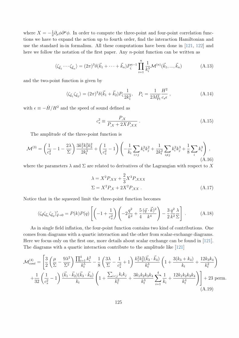
where X = −12∂µφ∂
µφ. In order to compute the three-point and four-point correlation func-
tions we have to expand the action up to fourth order, find the interaction Hamiltonian and
use the standard in-in formalism. All these computations have been done in [121, 122] and
here we follow the notation of the first paper. Any n-point function can be written as
〈ζ~k1· · · ζ~kn〉 = (2π)3δ(~k1 + · · ·+ ~kn)P n−1
ζ
n∏i=1
1
k3i
M(n)(~k1, ..., ~kn) (A.13)
and the two-point function is given by
〈ζ~k1ζ~k2〉 = (2π)3δ(~k1 + ~k2)Pζ
1
2k31
, Pζ =1
2M2Pl
H2
csε, (A.14)
with ε ≡ −H/H2 and the speed of sound defined as
c2s ≡
P,XP,X + 2XP,XX
. (A.15)
The amplitude of the three-point function is
M(3) =
(1
c2s
− 1− 2λ
Σ
)3k2
1k22k
23
2k3t
+
(1
c2s
− 1
)(− 1
kt
∑i>j
k2i k
2j +
1
2k2t
∑i 6=j
k2i k
3j +
1
8
∑i
k3i
),
(A.16)
where the parameters λ and Σ are related to derivatives of the Lagrangian with respect to X
λ = X2P,XX +2
3X3P,XXX
Σ = X2P,X + 2X2P,XX . (A.17)
Notice that in the squeezed limit the three-point function becomes
〈ζ~qζ~k1ζ~k2〉′~q→0 = P (k)P (q)
[(−1 +
1
c2s
)(−2
q2
k2+
5
4
(~q · ~k)2
k4
)− 3
2
q2
k2
λ
Σ
]. (A.18)
As in single field inflation, the four-point function contains two kind of contributions. One
comes from diagrams with a quartic interaction and the other from scalar-exchange diagrams.
Here we focus only on the first one, more details about scalar exchange can be found in [121].
The diagrams with a quartic interaction contribute to the amplitude like [121]
M(4)cont =
[3
2
(µ
Σ− 9λ2
Σ2
) ∏4i=1 k
2i
k5t
− 1
8
(3λ
Σ− 1
c2s
+ 1
)k2
1k22(~k3 · ~k4)
k3t
(1 +
3(k3 + k4)
kt+
12k3k4
k2t
)
+1
32
(1
c2s
− 1
)(~k1 · ~k2)(~k3 · ~k4)
kt
(1 +
∑i<j kikj
k2t
+3k1k2k3k4
k3t
4∑i=1
1
ki+
12k1k2k3k4
k4t
)]+ 23 perm.
(A.19)
125

with µ defined as:
µ =1
2X2P,XX + 2X3P,XXX +
2
3X4P,XXXX . (A.20)
When one of the momenta is much smaller we find
M(4)cont|~k4→0 =
[−1
2
(3λ
Σ− 1
c2s
+ 1
)k2
1k22(~k3 · ~k4)
k3t
(1 +
3k3
kt
)
+1
4
(1
c2s
− 1
)(~k1 · ~k2)(~k3 · ~k4)
kt
(1 +
k1k2 + k1k3 + k2k3
k2t
+3k1k2k3
k3t
)]+ 2 terms , (A.21)
where the two additional terms have the same form with ~k1 ↔ ~k3 and ~k2 ↔ ~k3. Notice
that since in the squeezed limit ~k1, ~k2 and ~k3 form a triangle, we can replace (~k1 · ~k2) →12(k2
3 − k21 − k2
2). We used this result to check the conformal consistency relation.
A.3 Resonant non-Gaussianities
In these models the inflaton potential has periodic modulation and they are motivated by
explicit string constructions of Monodromy Inflation [118]. It turns out that, at first order in
the size of modulation, all n-point functions can be analytically calculated [119, 120].
The (n+ 1)-point function reads [119, 120]
〈ζ~qζ~k1. . . ζ~kn〉 = (2π)3δ(~q + ~k1 + . . .+ ~kn)
(−Hφ
)n+1H2n−2
2q3∏n
i=1 2k3i
In+1 , (A.22)
where In+1 is given by the following in-in integral:
In+1 = −2 Im
∫ 0
−∞−iε
dη
η4V (n+1)(φ(η))(1− iqη)(1− ik1η) . . . (1− iknη)eiktη . (A.23)
Here kt = q +∑
i ki and V (n+1) is the (n + 1)th derivative of the potential, evaluated on
the unperturbed history φ(η). In resonant models, one starts from a trigonometric function
and therefore these derivatives are simply sines or cosines. Here we keep the discussion more
general, without specifying the form of the potential.
Notice that this result holds in the decoupling limit and neglecting diagrams with more
than one vertex. Corrections to the decoupling limit are suppressed by ε and they vanish in
the limit ε → 0 keeping constant the power spectrum of ζ [120]. Terms with more than one
vertex contain extra powers of the amplitude of the potential modulation. These corrections
eventually become sizeable for n-point functions with large n [119]. However, the consistency
relations must be satisfied independently by the single-vertex diagrams, as they are the only
ones proportional to the first power of the amplitude of the modulation. The integral over η
can be explicitly done in the saddle-point approximation, in the limit of many oscillations per
Hubble time [119, 120]. Since the consistency relations must hold independently of this limit,
and not only for oscillatory but for general potentials, here we prefer to keep the integral
form.
126

A.4 Khronon Inflation
Let us finally turn to an interesting example of Khronon Inflation [34]. In Khronon Inflation
the approximate shift symmetry of the inflaton
t→ t = t+ const , (A.24)
is promoted to the full time reparametrization invariance
t→ t(t) . (A.25)
This symmetry has been studied in the context of Horava gravity and its healthy extensions
[177, 178, 179]. In these references the scalar mode describing the preferred foliation has been
dubbed ‘khronon’.
We want to write an inflaton action in which the usual (approximate) symmetry φ→ φ+c
is promoted to the full invariance under field redefinition φ→ φ(φ). We are going to assume
an exact de Sitter metric and take the decoupling limit MPl →∞, in which the dynamics of
the scalar perturbations can be studied without considering the mixing with gravity. The time
dependent inflaton background defines a foliation and in the presence of φ reparameterization
invariance, the only invariant object is the 4-vector perpendicular to the foliation [179]
uµ =∂µφ√
−gαβ∂αφ∂βφ, (A.26)
which is indeed invariant under φ → φ(φ). At low energy the operators with the small-
est number of derivatives will dominate. One can show that the action to lowest order in
derivative—and any order in uµ—can thus be written as [34]
S =1
2
∫d4x√−g
(M2
PlR− 2Λ−M2λ (∇µu
µ − 3H)2 +M2αu
µuν∇µuρ∇νuρ), (A.27)
where Mα and Mλ are the two parameters of the model, besides the vacuum energy Λ which
is driving inflation.
A.4.1 The Power Spectrum
To calculate the power spectrum we expand the action (A.27) at second order. Using the field
redefinition symmetry we can assume to perturb around φ0 = t, i.e. φ (~x, t) = t + π (~x, t), in
an unperturbed de Sitter space, which is a good approximation in the decoupling limit
S2 =
∫d3x dη
(M2
α
2(∂π′)2 − M2
λ
2(∂2π)2
). (A.28)
This result is pretty unconventional. First of all, compared with the usual free-field action,
each term has two additional spatial derivatives. This is not worrisome as additional spatial
derivatives do not introduce extra pathological degrees of freedom. Second, the action does
127

not contain any η dependence so that the field is not sensitive to the expansion of the Universe
and behaves as in Minkowski space (though with a speed of sound which is, in general, different
from the speed of light). Actually these two peculiarities in some sense cancel each other to
give a scale-invariant spectrum. Indeed, we expect the mode functions to be of the Minkowski
form, but with an additional factor of 1/k because of the presence of the additional spatial
derivatives. It is easy to get the wavefunctions
πk(η) =1√2k3
1√MαMλ
e±iMλMα
kη , (A.29)
which give a scale-invariant spectrum for π at late times η → 0. The curvature perturbation
ζ is given by ζ = −Hπ so that
〈ζ~kζ~k′〉 = (2π)3δ(~k + ~k′)1
2k3
H2
MαMλ
. (A.30)
Notice that the scale invariance of the power spectrum (and of higher-order correlation func-
tions) can be justified by symmetry arguments [60], since we are in exact de Sitter and the
action is shift symmetric. Of course, a small tilt is induced if the field redefinition symmetry
is slightly broken.
Apart from other subtleties of this result (see the discussion in [34]), let us only notice
here that above feature leaves an interesting signature in the correlation functions of the
model. Indeed, the ”decaying” mode decays much slower than in the conventional case (as
1/a instead of 1/a3). This has remarkable consequences for the squeezed limits of correlation
functions: the standard single-field theorems hold, but only at first order in the momentum
of the long mode. In principle, it is possible to get 1/q2 divergence in the three-point function
in the squeezed limit. As it turns out in explicit calculations, this term is proportional to a
small breaking of the reparametrization symmetry and therefore practically unobservable.
A.4.2 The 3-point function
The interaction Lagrangian can be computed by expanding the action, equation (A.27), to
third order. We get, after several integrations by parts,
S3 =
∫d3x dη
1
a
[M2
λ
(2∂iπ
′∂iπ∂2π+π′∂i∂jπ∂i∂jπ
)+M2
α
(π′∂iπ
′′∂iπ−∂iπ′∂jπ∂i∂jπ)]. (A.31)
In order to compute the three-point function for ζ we use the relation ζ = −Hπ1
〈ζ~k1ζ~k2ζ~k3〉′ = 1∏
k3i
P 2ζ
[− k1
k2t
(k23~k1 · ~k2 + k2
2~k1 · ~k3)− k2
1
kt~k2 · ~k3 −
M2α
M2λ
k31
k2t
~k2 · ~k3
]+ cyclic perms. , (A.32)
1Additional non-linear terms in this relation either involve higher derivatives, which vanish outside of the
horizon, or are suppressed by slow-roll factors, see [43, 46].
128

where kt ≡ k1 + k2 + k3 and Pζ = H2/(2MαMλ) is the ζ power spectrum, eq. (A.30). All
the contributions but the last cannot be large and give an fNL ∼ 1. The contribution from
the last term on the other hand is proportional to M2α/M
2λ ≡ 1/c2
s. It is therefore a good
approximation to take the shape as equilateral. Its amplitude can be read from the expression
(A.32) above
f eqNL =
5
108
1
c2s
. (A.33)
Notice that this is the opposite of what happens in more conventional models with reduced
speed of sound (K-inflation), where the operator which reduces the speed of sound gives
f eq.NL ∝ −1/c2
s.
In the squeezed limit, this three-point function gives
〈ζ~qζ~k1ζ~k2〉′~q→0 =
P 2ζ
k3q3
1
4
M2α
M2λ
(q2
k2− 3
(~k · ~q)2
k4
). (A.34)
We can explicitly see that, after we average over the angles, the squeezed limit at order O(q2)
vanishes.
129

Appendix B
Derivation of the Consistency Relation
for Gravitational Waves
In this Appendix we are going to give some details on the derivation of the consistency relation
for short scalars and a long gravitational wave. We want to compute the average over the
long gravitational wave γmn(x) of the variation of the scalar n-point function induced by the
change of coordinates given in eq. (4.61). In order to simplify the notation let us define
Cij(~x+) = Aij(~x+)− 2Bijk(~x+)x+k ,
~P =∑i
~ki, 〈ζ~k1. . . ζ~kn〉 = δ(~P )M . (B.1)
Under this change of coordinates, the transformation of the n-point function is given by
δ〈ζ(~x1) . . . ζ(~xn)〉 =n∑a=1
(Cij(~x+)xaj∂ai +Bijk(~x+)xajxak∂ai) 〈ζ(~x1) . . . ζ(~xn)〉 . (B.2)
We can compute it term by term. The contribution from dilations is given by
δ〈ζ(~x1) . . . ζ(~xn)〉 ⊃n∑a=1
Cij(~x+)xaj∂ai〈ζ(~x1) . . . ζ(~xn)〉
=
∫dKn
∑a
Cij(~x+)δ(~P )Mkai∂kajei~k1·~x1+···+i~kn·~xn
=
∫dKnδ(~P )
(−∑a
Cij(~x+)kai∂kajM)ei~k1·~x1+···+i~kn·~xn . (B.3)
Here we used the fact that the tensor Cij is traceless and that a derivative on the delta
function can be rewritten as ∂Pjδ(~P ) leading to a term proportional to Piδ(~P ). Let us now
use the explicit expression for Cij
Cij(~x+) =1
2(1− x+
k ∂+k )γij(~x+) +
1
2
(x+k ∂
+i γjk(~x+)− x+
k ∂+j γik(~x+)
)(B.4)
130

and focus on the first term. Averaging over the long background mode γmn(x) we get
〈γmn(x)ζ(~x1) . . . ζ(~xn)〉 ⊃∫
d3~q
(2π)3dKnδ(~P )
(−∑a
kai∂kajM)
×∑s
εsmn(~q)εsij(~q)H2
q3
1
2(1− x+
k ∂+k )ei
~k1·~x1+···+i~kn·~xnei~q·~x−i~q·~x+ . (B.5)
Notice that (1 − x+k ∂
+k )e−i~q·~x+ = 1 + O(q2) which proves that there is no dependence of the
result on a choice of the point ~x+ at first order in the small momentum ~q. The second term of
eq. (B.4) has an additional dependence on ~x+ but it gives no contribution. After the averaging
over the long background mode γmn(x) the result is
〈γmn(x)ζ(~x1) . . . ζ(~xn)〉 ⊃∫
d3~q
(2π)3dKnδ(~P )
(−∑a
kai∂kajM)
×∑s
εsmn(~q)H2
q3
1
2
(iqjε
sik(~q)− iqiεsjk(~q)
)x+k e
i~k1·~x1+···+i~kn·~xnei~q·~x−i~q·~x+ . (B.6)
We can rewrite x+k in front of the exponent like i∂qk and do a partial integration. In the first
line in the integral nothing depends on ~q. The action on the second line will produce three
terms respectively proportional to
∼∑s
(∂qkεsmn(~q))
1
q3
(qjε
sik(~q)− qiεsjk(~q)
),
∼∑s
εsmn(~q)qkq5
(qjε
sik(~q)− qiεsjk(~q)
), (B.7)
∼∑s
εsmn(~q)1
q3
(εsij(~q) + qj∂qkε
sik(~q)− εsji(~q)− qi∂qkεsjk(~q)
).
The first term will vanish when we multiply both sides of the final equation by ε∗smn(~q) in order
to express everything in terms of the amplitudes. It is easy to see that ε∗smn(~q)∂qkεsmn(~q) = 0.
The second term is trivially zero because polarization tensors are transverse. To prove that
the last one is zero let us first note that one can write the polarization tensor like
εsaij (~ka) =1√2
(εPij(~ka) + isaε
Xij (~ka)) , εPij(
~ka) = zizj − uai uaj , εXij (~ka) = ziu
aj + zju
ai , (B.8)
and unit vectors ~z and ~ua are orthogonal to ~ka and each other [40]. Using these expressions
one can derive the following formula for the derivative of the polarization tensor
∂kjεslr(~k) = − 1
k2
(klε
sjr(~k) + krε
slj(~k)), (B.9)
which one can use to complete the proof.
131

We can focus now on the second part of the coordinate transformation. The variation of
the n-point function is
δ〈ζ(~x1) . . . ζ(~xn)〉 ⊃n∑a=1
Bijk(~x+)xajxak∂ai〈ζ(~x1) . . . ζ(~xn)〉
=
∫dKn
∑a
(−i)Bijk(~x+)δ(~P )Mkai∂kaj∂kakei~k1·~x1+···+i~kn·~xn
= −∫
dKn
∑a
iBijk(~x+)kai
(2∂kakδ(
~P ) + δ(~P )∂kaj
)∂kakMei
~k1·~x1+···+i~kn·~xn , (B.10)
where we have used similar tricks as before to get the final result. It is convenient to express
Bijk as a sum of two terms:
Bijk(~x+) =1
4
(∂+k γij(~x+)
)− 1
4
(∂+i γjk(~x+)− ∂+
j γik(~x+)). (B.11)
The term containing a derivative of the delta function in the variation of the n-point function
together with the first term in Bijk give:
〈γmn(x)ζ(~x1) . . . ζ(~xn)〉 ⊃∫
d3~q
(2π)3dKn
(−∑a
kai∂kajM)
× ~q · ∇δ(~P )∑s
εsmn(~q)εsij(~q)H2
q3
1
2ei~k1·~x1+···+i~kn·~xnei~q·~x−i~q·~x+ . (B.12)
The form of this contribution is the same as for dilations. When they sum up the final result
will be the same as for dilations but with a modified delta function δ(∑~ki + ~q). This means
that in all computations the n-point function has to be computed slightly off-shell. The two
additional terms that contain a derivative of the delta function will give a total contribution
proportional to∑
a
(kai∂kaj − kaj∂kai
)M, which is zero because the correlation functions are
rotationally invariant. Finally, the last part of the variation is
δ〈ζ(~x1) . . . ζ(~xn)〉 ⊃ −∫
dKnδ(~P )∑a
iBijk(~x+)kai∂kaj∂kakMei~k1·~x1+···+i~kn·~xn . (B.13)
After averaging over the long mode it gives the following contribution
〈γmn(x)ζ(~x1) . . . ζ(~xn)〉 ⊃∫
d3~q
(2π)3dKnδ(~P )
(−∑a
kai∂kaj∂kakM)
∑s
εsmn(~q)H2
q3
1
4
(qkε
sij(~q)− qiεsjk(~q) + qjε
sik(~q)
)ei~q·~x+i~k1·~x1+···+i~kn·~xn . (B.14)
Summing up all nonzero terms and going to momentum space on the left hand side, we
get the consistency relation for a background tensor mode:
〈γs~qζ~k1. . . ζ~kn〉
′q→0 = −1
2Pγ(q)
∑a
εsij(~q)
(kai + kai(~q · ~∂ka)−
1
2(~q · ~ka)∂kai
)∂kaj〈ζ~k1
. . . ζ~kn〉′ .
(B.15)
132

Appendix C
An Example of the Equivalence
Principle Violation
In this section we are going to study a toy model in which the Universe is composed of two
non-relativistic fluids A and B, with the latter coupled to a scalar field mediating a fifth force.
For example, the two fluids could be baryons and dark matter but, with some modifications
that we will discuss below, the model can also describe two populations of astrophysical
objects, say different types of galaxies. If the scalar field ϕ has a negligible time evolution,
the continuity equations of the two fluids are the same,
δ′X + ~∇ · [(1 + δX)~vX ] = 0 , X = A,B . (C.1)
The Euler equation of B contains the fifth force, whose coupling is parameterized by α,
~v′A +H~vA + (~vA · ~∇)~vA = −~∇Φ , (C.2)
~v′B +H~vB + (~vB · ~∇)~vB = −~∇Φ− α~∇ϕ , (C.3)
where H ≡ ∂ηa/a is the comoving Hubble parameter. To close this system of equations we
need Poisson’s equation and the evolution equation of the scalar field. Assuming that the
scalar field stress-energy tensor is negligible, only matter appears as a source in the Poisson’s
equation,
∇2Φ = 4πGρm δ = 4πGρm (wAδA + wBδB) , (C.4)
where ρm is the total matter density and wX ≡ ρX/ρm is the density fraction of the X species.
Moreover, in the non-relativistic approximation we can neglect time derivatives in comparison
with spatial gradients and the equation for the scalar field reads
∇2ϕ = α · 8πGρmwBδB , (C.5)
where we have neglected the mass of the scalar field, assuming we are on scales much shorter
than its Compton wavelength.
133

Let us start with the linear theory and, following [180], look for two of the four independent
solutions of the system in which the density and the velocity of the species B differ from those
of the species A by a (possibly time-dependent) bias factor b,
δ(A)~k
(η) = D(η) δ0(~k) , (C.6)
θ(A)~k
(η) = −H(η)f(η)δ(A)~k
(η) , (C.7)
δ(B)~k
(η) = b(η)δ(A)~k
(η) , (C.8)
θ(B)~k
(η) = −H(η)f(η)δ(B)~k
(η) , (C.9)
where we have defined θ(X) ≡ ~∇ · ~vX and δ0(~k) is a Gaussian random variable. Plugging this
ansatz in eqs. (C.1)–(C.5) and using the background Friedmann equations for a flat universe,
we find, at linear order,
f =d lnD
d ln a, (C.10)
df
d ln a+ f 2 +
(2− 3
2Ωm
)f − 3
2Ωm(wA + wBb) = 0 , (C.11)
db
d ln a= 0 , (C.12)
wBb+ wA
(1− 1
b
)− wB(1 + 2α2) = 0 . (C.13)
Using eqs. (C.10) and (C.11), the linear growth factor D satisfies a second-order equation,
d2D
d ln a2+
(2− 3
2Ωm
)dD
d ln a− 3
2Ωm(wA + wBb)D = 0 , (C.14)
whose growing and decaying solutions are D+ and D−. Note that eq. (C.12) implies that
the bias b is time independent. In the absence of EP violation (α = 0) we get b = 1 (using
wA + wB = 1) and we recover from eq. (C.14) the usual evolution of the growth of matter
perturbations.
Following [102, 181], we introduce y ≡ lnD+ as the time variable. Defining the field
multiplet
Ψa ≡
δ(A)
−θ(A)/Hf+
δ(B)
−θ(B)/Hf+
, (C.15)
the equations of motion of the two fluids can be then written in a very compact form as
∂yΨa(~k) + ΩabΨb(~k) = γabcΨb(~k1)Ψc(~k2) , (C.16)
where integration over ~k1 and ~k2 is implied on the right-hand side. The entries of γabc vanish
134

except for
γ121 = γ343 = (2π)3δD(~k − ~k1 − ~k2)~k1 · (~k1 + ~k2)
k21
,
γ222 = γ444 = (2π)3δD(~k − ~k1 − ~k2)~k1 · ~k2(~k1 + ~k2)2
2k21k
22
,
(C.17)
the matrix Ωab reads
Ωab =
0 −1 0 0
−32
Ωmf2+wA
32
Ωmf2+
(wA + bwB)− 1 −32
Ωmf2+wB 0
0 0 0 −1
−32
Ωmf2+wA 0 −3
2Ωmf2+
(wBb+ wA(1− 1
b
)) 3
2Ωmf2+
(wA + bwB)− 1
,
(C.18)
and we have employed eq. (C.13) to replace the dependence on α2 by a dependence on the
bias b. The solution of eq. (C.16) can be formally written as
Ψa(y) = gab(y)φb +
∫ y
0
dy′gab(y − y′)γbcdΨc(y′)Ψd(y
′) , (C.19)
where φb is the initial condition, φb = Ψb(y = 0), and gab(y) is the linear propagator which is
given by [102]
gab(y) =1
2πi
∫ ξ+i∞
ξ−i∞dω (ωI + Ω)−1
ab eωy , (C.20)
where ξ is a real number larger than the real parts of the poles of (ωI + Ω)−1.
In the following we consider small couplings to the fifth force, α2 1, which by virtue
of eq. (C.13) implies b ' 1. In this case, it is reasonable to use the approximation f 2+ ' Ωm,
which for b = 1 is very good throughout the whole evolution [182]. We choose to use this
approximation because it considerably simplifies the presentation but one can easily drop
it and make an exact computation. The linear evolution is characterized by four modes.
Expanding for small b − 1, apart from the “adiabatic” growing and decaying modes already
introduced above, respectively going as D+ = ey and D− = e−32
[1+wB(b−1)]y, one finds two
“isodensity” modes, one decaying as Di = e−12
[1+3(1+wA)(b−1)]y and an almost constant one
going as Dc = e3wA(b−1)α2y.(1)
We are interested in the equal-time 3-point function involving the two species. In partic-
ular, we compute
〈δ~k3(η)δ
(A)~k1
(η)δ(B)~k2
(η)〉 = wA〈Ψ1(k3, η)Ψ1(k1, η)Ψ3(k2, η)〉+ wB〈Ψ3(k3, η)Ψ1(k1, η)Ψ3(k2, η)〉 ,(C.21)
1With an abuse of language, we denote the modes (+) and (−) as adiabatic and (i) and (c) as isodensity
even though, strictly speaking, they do not correspond to the usual notion of adiabatic and isocurvature.
Indeed, (+) and (−) correspond to δA = δB/b and not to δA = δB as in the standard adiabatic case, while
(i) and (c) yield wAδ(A) + bwBδ
(B) = 0 instead of wAδ(A) + wBδ
(B) = 0 which one finds in the standard
isodensity case (see [140] for a discussion of adiabatic and isodensity modes in the standard case b = 1).
135

where δ ≡ wAδ(A) + wBδ
(B). The calculation can be straightforwardly done at tree level by
perturbatively expanding the solution (C.19) as Ψa = Ψ(1)a + Ψ
(2)a + . . ., which up to second
order in δ0 yields
Ψ(1)a (y) = gab(y)φb ,
Ψ(2)a (y) =
∫ y
0
dy′gab(y − y′)γbcdΨ(1)c (y′)Ψ
(1)d (y′) ,
(C.22)
and by applying Wick’s theorem over the Gaussian initial conditions. In the squeezed limit,
the expression for (C.21) simplifies considerably. Assuming that the initial conditions are in
the most growing mode, i.e. they are given by φa(~k) = uaδ0(~k) with ua = (1, 1, b, b), at leading
order in b− 1 one finds
limq→0〈δ~q(η)δ
(A)~k1
(η)δ(B)~k2
(η)〉 ' −(b−1)P (q, η)P (k, 0)~k · ~qq2
∫ y
0
dy′e2y′[g11 +g12−g31−g32
](y−y′) ,
(C.23)
which shows that the long wavelength adiabatic evolution has no effect on the 3-point function2
[140, 141]. Retaining the most growing contribution and using b ' 1+2wBα2 one finally finds
limq→0〈δ~q(η)δ
(A)~k1
(η)δ(B)~k2
(η)〉′ ' 7
5wB α
2~k · ~qq2
P (q, η)PAB(k, η) . (C.24)
2For b = 1 one finds g(+)11 = g
(+)31 , g
(+)12 = g
(+)32 , g
(−)11 = g
(−)31 and g
(−)12 = g
(−)32 .
136

Bibliography
[1] George F. Smoot, C.L. Bennett, A. Kogut, E.L. Wright, J. Aymon, et al. Structure in
the COBE differential microwave radiometer first year maps. Astrophys.J., 396:L1–L5,
1992.
[2] A. Balbi, P. Ade, J. Bock, J. Borrill, A. Boscaleri, et al. Constraints on cosmological
parameters from MAXIMA-1. Astrophys.J., 545:L1–L4, 2000.
[3] P. de Bernardis et al. A Flat universe from high resolution maps of the cosmic microwave
background radiation. Nature, 404:955–959, 2000.
[4] Peter M. Garnavich et al. Supernova limits on the cosmic equation of state. Astrophys.J.,
509:74–79, 1998.
[5] Jochen Weller and Andreas Albrecht. Future supernovae observations as a probe of
dark energy. Phys.Rev., D65:103512, 2002.
[6] W.L. Freedman et al. Final results from the Hubble Space Telescope key project to
measure the Hubble constant. Astrophys.J., 553:47–72, 2001.
[7] G. Hinshaw et al. Nine-Year Wilkinson Microwave Anisotropy Probe (WMAP) Obser-
vations: Cosmological Parameter Results. Astrophys.J.Suppl., 208:19, 2013.
[8] Paolo Creminelli, Leonardo Senatore, Matias Zaldarriaga, and Max Tegmark. Limits
on fNL parameters from WMAP 3yr data. JCAP, 0703:005, 2007.
[9] Kendrick M. Smith, Leonardo Senatore, and Matias Zaldarriaga. Optimal limits on
f localNL from WMAP 5-year data. JCAP, 0909:006, 2009.
[10] Leonardo Senatore, Kendrick M. Smith, and Matias Zaldarriaga. Non-Gaussianities in
Single Field Inflation and their Optimal Limits from the WMAP 5-year Data. JCAP,
1001:028, 2010.
[11] P.A.R. Ade et al. Planck 2013 results. XVI. Cosmological parameters. As-
tron.Astrophys., 2014.
[12] P.A.R. Ade et al. Planck 2013 results. XXII. Constraints on inflation. 2013.
137

[13] P.A.R. Ade et al. Planck 2013 Results. XXIV. Constraints on primordial non-
Gaussianity. 2013.
[14] Uros Seljak and Matias Zaldarriaga. Signature of gravity waves in polarization of the
microwave background. Phys.Rev.Lett., 78:2054–2057, 1997.
[15] Marc Kamionkowski, Arthur Kosowsky, and Albert Stebbins. A Probe of primordial
gravity waves and vorticity. Phys.Rev.Lett., 78:2058–2061, 1997.
[16] D. Hanson et al. Detection of B-mode Polarization in the Cosmic Microwave Background
with Data from the South Pole Telescope. Phys.Rev.Lett., 111(14):141301, 2013.
[17] P.A.R. Ade et al. A Measurement of the Cosmic Microwave Background B-Mode Po-
larization Power Spectrum at Sub-Degree Scales with POLARBEAR. 2014.
[18] P.A.R. Ade et al. Detection of B-Mode Polarization at Degree Angular Scales by BI-
CEP2. Phys.Rev.Lett., 112:241101, 2014.
[19] Raphael Flauger, J. Colin Hill, and David N. Spergel. Toward an Understanding of
Foreground Emission in the BICEP2 Region. 2014.
[20] Michael J. Mortonson and Uro Seljak. A joint analysis of Planck and BICEP2 B modes
including dust polarization uncertainty. 2014.
[21] Max Tegmark et al. Cosmological parameters from SDSS and WMAP. Phys.Rev.,
D69:103501, 2004.
[22] Daniel J. Eisenstein et al. Detection of the baryon acoustic peak in the large-scale
correlation function of SDSS luminous red galaxies. Astrophys.J., 633:560–574, 2005.
[23] Nicolas G. Busca, Timothee Delubac, James Rich, Stephen Bailey, Andreu Font-
Ribera, et al. Baryon Acoustic Oscillations in the Ly-α forest of BOSS quasars. As-
tron.Astrophys., 552:A96, 2013.
[24] Luca Amendola et al. Cosmology and fundamental physics with the Euclid satellite.
Living Rev.Rel., 16:6, 2013.
[25] Clifford Cheung, Paolo Creminelli, A. Liam Fitzpatrick, Jared Kaplan, and Leonardo
Senatore. The Effective Field Theory of Inflation. JHEP, 0803:014, 2008.
[26] Leonardo Senatore and Matias Zaldarriaga. The Effective Field Theory of Multifield
Inflation. JHEP, 1204:024, 2012.
[27] Paolo Creminelli, Guido D’Amico, Jorge Norena, and Filippo Vernizzi. The Effective
Theory of Quintessence: the w < −1 Side Unveiled. JCAP, 0902:018, 2009.
138

[28] Federico Piazza and Filippo Vernizzi. Effective Field Theory of Cosmological Pertur-
bations. Class.Quant.Grav., 30:214007, 2013.
[29] Daniel Baumann, Alberto Nicolis, Leonardo Senatore, and Matias Zaldarriaga. Cosmo-
logical Non-Linearities as an Effective Fluid. JCAP, 1207:051, 2012.
[30] John Joseph M. Carrasco, Mark P. Hertzberg, and Leonardo Senatore. The Effective
Field Theory of Cosmological Large Scale Structures. JHEP, 1209:082, 2012.
[31] Enrico Pajer and Matias Zaldarriaga. On the Renormalization of the Effective Field
Theory of Large Scale Structures. JCAP, 1308:037, 2013.
[32] John Joseph M. Carrasco, Simon Foreman, Daniel Green, and Leonardo Senatore. The
Effective Field Theory of Large Scale Structures at Two Loops. JCAP, 1407:057, 2014.
[33] Rafael A. Porto, Leonardo Senatore, and Matias Zaldarriaga. The Lagrangian-space
Effective Field Theory of Large Scale Structures. JCAP, 1405:022, 2014.
[34] Paolo Creminelli, Jorge Norena, Manuel Pena, and Marko Simonovic. Khronon inflation.
JCAP, 1211:032, 2012.
[35] Paolo Creminelli, Guido D’Amico, Marcello Musso, Jorge Norena, and Enrico
Trincherini. Galilean symmetry in the effective theory of inflation: new shapes of
non-Gaussianity. JCAP, 1102:006, 2011.
[36] Paolo Creminelli, Razieh Emami, Marko Simonovic, and Gabriele Trevisan. ISO(4,1)
Symmetry in the EFT of Inflation. JCAP, 1307:037, 2013.
[37] Andrei D. Linde and Viatcheslav F. Mukhanov. Nongaussian isocurvature perturbations
from inflation. Phys.Rev., D56:535–539, 1997.
[38] David H. Lyth, Carlo Ungarelli, and David Wands. The Primordial density perturbation
in the curvaton scenario. Phys.Rev., D67:023503, 2003.
[39] Ignatios Antoniadis, Pawel O. Mazur, and Emil Mottola. Conformal Invariance, Dark
Energy, and CMB Non-Gaussianity. JCAP, 1209:024, 2012.
[40] Juan M. Maldacena and Guilherme L. Pimentel. On graviton non-Gaussianities during
inflation. JHEP, 1109:045, 2011.
[41] Paolo Creminelli. Conformal invariance of scalar perturbations in inflation. Phys.Rev.,
D85:041302, 2012.
[42] Ian Low and Aneesh V. Manohar. Spontaneously broken space-time symmetries and
Goldstone’s theorem. Phys.Rev.Lett., 88:101602, 2002.
139

[43] Juan Martin Maldacena. Non-Gaussian features of primordial fluctuations in single field
inflationary models. JHEP, 0305:013, 2003.
[44] Steven Weinberg. Adiabatic modes in cosmology. Phys.Rev., D67:123504, 2003.
[45] Paolo Creminelli and Matias Zaldarriaga. Single field consistency relation for the 3-point
function. JCAP, 0410:006, 2004.
[46] Clifford Cheung, A. Liam Fitzpatrick, Jared Kaplan, and Leonardo Senatore. On the
consistency relation of the 3-point function in single field inflation. JCAP, 0802:021,
2008.
[47] Paolo Creminelli, Guido D’Amico, Marcello Musso, and Jorge Norena. The (not so)
squeezed limit of the primordial 3-point function. JCAP, 1111:038, 2011.
[48] Paolo Creminelli, Jorge Norena, and Marko Simonovic. Conformal consistency relations
for single-field inflation. JCAP, 1207:052, 2012.
[49] Valentin Assassi, Daniel Baumann, and Daniel Green. On Soft Limits of Inflationary
Correlation Functions. JCAP, 1211:047, 2012.
[50] Kurt Hinterbichler, Lam Hui, and Justin Khoury. An Infinite Set of Ward Identities for
Adiabatic Modes in Cosmology. JCAP, 1401:039, 2014.
[51] Walter D. Goldberger, Lam Hui, and Alberto Nicolis. One-particle-irreducible consis-
tency relations for cosmological perturbations. Phys.Rev., D87(10):103520, 2013.
[52] Guilherme L. Pimentel. Inflationary Consistency Conditions from a Wavefunctional
Perspective. JHEP, 1402:124, 2014.
[53] Lasha Berezhiani and Justin Khoury. Slavnov-Taylor Identities for Primordial Pertur-
bations. JCAP, 1402:003, 2014.
[54] Hael Collins, R. Holman, and Tereza Vardanyan. A Cosmological Slavnov-Taylor Iden-
tity. 2014.
[55] A. Kehagias and A. Riotto. Operator Product Expansion of Inflationary Correlators
and Conformal Symmetry of de Sitter. Nucl.Phys., B864:492–529, 2012.
[56] A. Kehagias and A. Riotto. The Four-point Correlator in Multifield Inflation, the
Operator Product Expansion and the Symmetries of de Sitter. Nucl.Phys., B868:577–
595, 2013.
[57] Koenraad Schalm, Gary Shiu, and Ted van der Aalst. Consistency condition for inflation
from (broken) conformal symmetry. JCAP, 1303:005, 2013.
140

[58] Adam Bzowski, Paul McFadden, and Kostas Skenderis. Holography for inflation using
conformal perturbation theory. JHEP, 1304:047, 2013.
[59] V.A. Rubakov. Harrison-Zeldovich spectrum from conformal invariance. JCAP,
0909:030, 2009.
[60] Paolo Creminelli, Alberto Nicolis, and Enrico Trincherini. Galilean Genesis: An Alter-
native to inflation. JCAP, 1011:021, 2010.
[61] Kurt Hinterbichler and Justin Khoury. The Pseudo-Conformal Universe: Scale Invari-
ance from Spontaneous Breaking of Conformal Symmetry. JCAP, 1204:023, 2012.
[62] Kurt Hinterbichler, Austin Joyce, and Justin Khoury. Non-linear Realizations of Confor-
mal Symmetry and Effective Field Theory for the Pseudo-Conformal Universe. JCAP,
1206:043, 2012.
[63] Paolo Creminelli, Austin Joyce, Justin Khoury, and Marko Simonovic. Consistency
Relations for the Conformal Mechanism. JCAP, 1304:020, 2013.
[64] Paolo Creminelli, Cyril Pitrou, and Filippo Vernizzi. The CMB bispectrum in the
squeezed limit. JCAP, 1111:025, 2011.
[65] A. Kehagias and A. Riotto. Symmetries and Consistency Relations in the Large Scale
Structure of the Universe. Nucl.Phys., B873:514–529, 2013.
[66] Marco Peloso and Massimo Pietroni. Galilean invariance and the consistency relation
for the nonlinear squeezed bispectrum of large scale structure. JCAP, 1305:031, 2013.
[67] Paolo Creminelli, Jorge Norena, Marko Simonovic, and Filippo Vernizzi. Single-Field
Consistency Relations of Large Scale Structure. JCAP, 1312:025, 2013.
[68] Marco Peloso and Massimo Pietroni. Ward identities and consistency relations for the
large scale structure with multiple species. JCAP, 1404:011, 2014.
[69] Paolo Creminelli, Jerome Gleyzes, Marko Simonovic, and Filippo Vernizzi. Single-Field
Consistency Relations of Large Scale Structure. Part II: Resummation and Redshift
Space. JCAP, 1402:051, 2014.
[70] Paolo Creminelli, Jerome Gleyzes, Lam Hui, Marko Simonovic, and Filippo Vernizzi.
Single-Field Consistency Relations of Large Scale Structure. Part III: Test of the Equiv-
alence Principle. 2013.
[71] Alexandros Kehagias, Jorge Norea, Hideki Perrier, and Antonio Riotto. Consequences
of Symmetries and Consistency Relations in the Large-Scale Structure of the Universe
for Non-local bias and Modified Gravity. Nucl.Phys., B883:83–106, 2014.
[72] Patrick Valageas. Consistency relations of large-scale structures. 2013.
141

[73] Patrick Valageas. Angular averaged consistency relations of large-scale structures.
Phys.Rev., D89:123522, 2014.
[74] Alex Kehagias, Hideki Perrier, and Antonio Riotto. Equal-time Consistency Relations
in the Large-Scale Structure of the Universe. 2013.
[75] Bart Horn, Lam Hui, and Xiao Xiao. Soft-Pion Theorems for Large Scale Structure.
2014.
[76] Scott Dodelson. Modern cosmology. 2003.
[77] V. Mukhanov. Physical foundations of cosmology. 2005.
[78] Steven Weinberg. Cosmology. 2008.
[79] Alexei A. Starobinsky. A New Type of Isotropic Cosmological Models Without Singu-
larity. Phys.Lett., B91:99–102, 1980.
[80] Alan H. Guth. The Inflationary Universe: A Possible Solution to the Horizon and
Flatness Problems. Phys.Rev., D23:347–356, 1981.
[81] Andrei D. Linde. A New Inflationary Universe Scenario: A Possible Solution of the Hori-
zon, Flatness, Homogeneity, Isotropy and Primordial Monopole Problems. Phys.Lett.,
B108:389–393, 1982.
[82] Andrei D. Linde. Chaotic Inflation. Phys.Lett., B129:177–181, 1983.
[83] Andreas Albrecht and Paul J. Steinhardt. Cosmology for Grand Unified Theories with
Radiatively Induced Symmetry Breaking. Phys.Rev.Lett., 48:1220–1223, 1982.
[84] Viatcheslav F. Mukhanov and G. V. Chibisov. Quantum Fluctuation and Nonsingular
Universe. (In Russian). JETP Lett., 33:532–535, 1981.
[85] S.W. Hawking. The Development of Irregularities in a Single Bubble Inflationary Uni-
verse. Phys.Lett., B115:295, 1982.
[86] Alan H. Guth and S.Y. Pi. Fluctuations in the New Inflationary Universe.
Phys.Rev.Lett., 49:1110–1113, 1982.
[87] Alexei A. Starobinsky. Dynamics of Phase Transition in the New Inflationary Universe
Scenario and Generation of Perturbations. Phys.Lett., B117:175–178, 1982.
[88] James M. Bardeen, Paul J. Steinhardt, and Michael S. Turner. Spontaneous Creation
of Almost Scale - Free Density Perturbations in an Inflationary Universe. Phys.Rev.,
D28:679, 1983.
[89] Viatcheslav F. Mukhanov. Gravitational Instability of the Universe Filled with a Scalar
Field. JETP Lett., 41:493–496, 1985.
142

[90] Daniel Baumann. TASI Lectures on Inflation. 2009.
[91] Leonardo Senatore and Matias Zaldarriaga. On Loops in Inflation. JHEP, 1012:008,
2010.
[92] Leonardo Senatore and Matias Zaldarriaga. On Loops in Inflation II: IR Effects in
Single Clock Inflation. JHEP, 1301:109, 2013.
[93] Guilherme L. Pimentel, Leonardo Senatore, and Matias Zaldarriaga. On Loops in
Inflation III: Time Independence of zeta in Single Clock Inflation. JHEP, 1207:166,
2012.
[94] Leonardo Senatore and Matias Zaldarriaga. The constancy of ζ in single-clock Inflation
at all loops. JHEP, 1309:148, 2013.
[95] Valentin Assassi, Daniel Baumann, and Daniel Green. Symmetries and Loops in Infla-
tion. JHEP, 1302:151, 2013.
[96] Steven Weinberg. Quantum contributions to cosmological correlations. Phys.Rev.,
D72:043514, 2005.
[97] Jaume Garriga and Viatcheslav F. Mukhanov. Perturbations in k-inflation. Phys.Lett.,
B458:219–225, 1999.
[98] Daniel Babich, Paolo Creminelli, and Matias Zaldarriaga. The Shape of non-
Gaussianities. JCAP, 0408:009, 2004.
[99] Paolo Creminelli. On non-Gaussianities in single-field inflation. JCAP, 0310:003, 2003.
[100] Nima Arkani-Hamed, Paolo Creminelli, Shinji Mukohyama, and Matias Zaldarriaga.
Ghost inflation. JCAP, 0404:001, 2004.
[101] F. Bernardeau, S. Colombi, E. Gaztanaga, and R. Scoccimarro. Large scale structure
of the universe and cosmological perturbation theory. Phys.Rept., 367:1–248, 2002.
[102] Martin Crocce and Roman Scoccimarro. Renormalized cosmological perturbation the-
ory. Phys.Rev., D73:063519, 2006.
[103] Massimo Pietroni, Gianpiero Mangano, Ninetta Saviano, and Matteo Viel. Coarse-
Grained Cosmological Perturbation Theory. JCAP, 1201:019, 2012.
[104] Alessandro Manzotti, Marco Peloso, Massimo Pietroni, Matteo Viel, and Francisco
Villaescusa-Navarro. A coarse grained perturbation theory for the Large Scale Structure,
with cosmology and time independence in the UV. 2014.
[105] Nick Kaiser. On the Spatial correlations of Abell clusters. Astrophys.J., 284:L9–L12,
1984.
143
[106] Edmund Bertschinger. Cosmological dynamics: Course 1. 1993.
[107] Sabino Matarrese, Silvia Mollerach, and Marco Bruni. Second order perturbations of
the Einstein-de Sitter universe. Phys.Rev., D58:043504, 1998.
[108] Lotfi Boubekeur, Paolo Creminelli, Jorge Norena, and Filippo Vernizzi. Action approach
to cosmological perturbations: the 2nd order metric in matter dominance. JCAP,
0808:028, 2008.
[109] A. Liam Fitzpatrick, Leonardo Senatore, and Matias Zaldarriaga. Contributions to the
Dark Matter 3-Pt Function from the Radiation Era. JCAP, 1005:004, 2010.
[110] Gia Dvali, Andrei Gruzinov, and Matias Zaldarriaga. A new mechanism for generating
density perturbations from inflation. Phys.Rev., D69:023505, 2004.
[111] N. Bartolo, E. Komatsu, Sabino Matarrese, and A. Riotto. Non-Gaussianity from
inflation: Theory and observations. Phys.Rept., 402:103–266, 2004.
[112] Xingang Chen, Hassan Firouzjahi, Mohammad Hossein Namjoo, and Misao Sasaki.
A Single Field Inflation Model with Large Local Non-Gaussianity. Europhys.Lett.,
102:59001, 2013.
[113] R. Holman and Andrew J. Tolley. Enhanced Non-Gaussianity from Excited Initial
States. JCAP, 0805:001, 2008.
[114] Raphael Flauger, Daniel Green, and Rafael A. Porto. On squeezed limits in single-field
inflation. Part I. JCAP, 1308:032, 2013.
[115] Lasha Berezhiani and Justin Khoury. On the Initial State and Consistency Relations.
2014.
[116] Leonardo Senatore and Matias Zaldarriaga. A Naturally Large Four-Point Function in
Single Field Inflation. JCAP, 1101:003, 2011.
[117] Xingang Chen, Min-xin Huang, Shamit Kachru, and Gary Shiu. Observational signa-
tures and non-Gaussianities of general single field inflation. JCAP, 0701:002, 2007.
[118] Liam McAllister, Eva Silverstein, and Alexander Westphal. Gravity Waves and Linear
Inflation from Axion Monodromy. Phys.Rev., D82:046003, 2010.
[119] Louis Leblond and Enrico Pajer. Resonant Trispectrum and a Dozen More Primordial
N-point functions. JCAP, 1101:035, 2011.
[120] Siavosh R. Behbahani, Anatoly Dymarsky, Mehrdad Mirbabayi, and Leonardo Senatore.
(Small) Resonant non-Gaussianities: Signatures of a Discrete Shift Symmetry in the
Effective Field Theory of Inflation. JCAP, 1212:036, 2012.
144

[121] Xingang Chen, Bin Hu, Min-xin Huang, Gary Shiu, and Yi Wang. Large Primordial
Trispectra in General Single Field Inflation. JCAP, 0908:008, 2009.
[122] Frederico Arroja, Shuntaro Mizuno, Kazuya Koyama, and Takahiro Tanaka. On the
full trispectrum in single field DBI-inflation. Phys.Rev., D80:043527, 2009.
[123] David Seery, James E. Lidsey, and Martin S. Sloth. The inflationary trispectrum. JCAP,
0701:027, 2007.
[124] David Seery, Martin S. Sloth, and Filippo Vernizzi. Inflationary trispectrum from gravi-
ton exchange. JCAP, 0903:018, 2009.
[125] Enrico Pajer and Matias Zaldarriaga. A New Window on Primordial non-Gaussianity.
Phys.Rev.Lett., 109:021302, 2012.
[126] Paolo Creminelli, Ashley Perko, Leonardo Senatore, Marko Simonovic, and Gabriele
Trevisan. The Physical Squeezed Limit: Consistency Relations at Order q2. JCAP,
1311:015, 2013.
[127] Mohsen Alishahiha, Eva Silverstein, and David Tong. DBI in the sky. Phys.Rev.,
D70:123505, 2004.
[128] Diana Lopez Nacir, Rafael A. Porto, Leonardo Senatore, and Matias Zaldarriaga. Dis-
sipative effects in the Effective Field Theory of Inflation. JHEP, 1201:075, 2012.
[129] Austin Joyce, Justin Khoury, and Marko Simonovic. Multiple soft limits of cosmological
correlation functions, to appear.
[130] P. Di Francesco, P. Mathieu, and D. Senechal. Conformal field theory. 1997.
[131] Xingang Chen, Min-xin Huang, and Gary Shiu. The Inflationary Trispectrum for Models
with Large Non-Gaussianities. Phys.Rev., D74:121301, 2006.
[132] Leonardo Senatore and Matias Zaldarriaga. A Note on the Consistency Condition of
Primordial Fluctuations. JCAP, 1208:001, 2012.
[133] Nima Arkani-Hamed, Freddy Cachazo, and Jared Kaplan. What is the Simplest Quan-
tum Field Theory? JHEP, 1009:016, 2010.
[134] Kurt Hinterbichler, Lam Hui, and Justin Khoury. Conformal Symmetries of Adiabatic
Modes in Cosmology. JCAP, 1208:017, 2012.
[135] Alberto Nicolis, Riccardo Rattazzi, and Enrico Trincherini. The Galileon as a local
modification of gravity. Phys.Rev., D79:064036, 2009.
[136] Clare Burrage, Claudia de Rham, David Seery, and Andrew J. Tolley. Galileon inflation.
JCAP, 1101:014, 2011.
145

[137] C. Deffayet, Gilles Esposito-Farese, and A. Vikman. Covariant Galileon. Phys.Rev.,
D79:084003, 2009.
[138] Lasha Berezhiani, Justin Khoury, and Junpu Wang. Non-Trivial Checks of Novel Con-
sistency Relations. JCAP, 1406:056, 2014.
[139] Dmitriy Tseliakhovich and Christopher Hirata. Relative velocity of dark matter and
baryonic fluids and the formation of the first structures. Phys.Rev., D82:083520, 2010.
[140] Francis Bernardeau, Nicolas Van de Rijt, and Filippo Vernizzi. Resummed propa-
gators in multi-component cosmic fluids with the eikonal approximation. Phys.Rev.,
D85:063509, 2012.
[141] Francis Bernardeau, Nicolas Van de Rijt, and Filippo Vernizzi. Power spectra in the
eikonal approximation with adiabatic and non-adiabatic modes. Phys.Rev., D87:043530,
2013.
[142] Bhuvnesh Jain and Edmund Bertschinger. Selfsimilar evolution of cosmological density
fluctuations. Astrophys.J., 456:43, 1996.
[143] Roman Scoccimarro and Joshua Frieman. Loop corrections in nonlinear cosmological
perturbation theory. Astrophys.J.Suppl., 105:37, 1996.
[144] Diego Blas, Mathias Garny, and Thomas Konstandin. On the non-linear scale of cos-
mological perturbation theory. JCAP, 1309:024, 2013.
[145] John Joseph M. Carrasco, Simon Foreman, Daniel Green, and Leonardo Senatore. The
2-loop matter power spectrum and the IR-safe integrand. JCAP, 1407:056, 2014.
[146] Uros Seljak and Patrick McDonald. Distribution function approach to redshift space
distortions. JCAP, 1111:039, 2011.
[147] Zvonimir Vlah, Uros Seljak, Patrick McDonald, Teppei Okumura, and Tobias Baldauf.
Distribution function approach to redshift space distortions. Part IV: perturbation the-
ory applied to dark matter. JCAP, 1211:009, 2012.
[148] Tobias Baldauf, Uros Seljak, and Leonardo Senatore. Primordial non-Gaussianity in
the Bispectrum of the Halo Density Field. JCAP, 1104:006, 2011.
[149] Justin Khoury. Les Houches Lectures on Physics Beyond the Standard Model of Cos-
mology. 2013.
[150] Lam Hui, Alberto Nicolis, and Christopher Stubbs. Equivalence Principle Implications
of Modified Gravity Models. Phys.Rev., D80:104002, 2009.
[151] Justin Khoury and Amanda Weltman. Chameleon fields: Awaiting surprises for tests
of gravity in space. Phys.Rev.Lett., 93:171104, 2004.
146

[152] Kurt Hinterbichler and Justin Khoury. Symmetron Fields: Screening Long-Range
Forces Through Local Symmetry Restoration. Phys.Rev.Lett., 104:231301, 2010.
[153] Massimo Pietroni. Dark energy condensation. Phys.Rev., D72:043535, 2005.
[154] Keith A. Olive and Maxim Pospelov. Environmental dependence of masses and coupling
constants. Phys.Rev., D77:043524, 2008.
[155] Junpu Wang, Lam Hui, and Justin Khoury. No-Go Theorems for Generalized
Chameleon Field Theories. Phys.Rev.Lett., 109:241301, 2012.
[156] Philippe Brax, Anne-Christine Davis, and Baojiu Li. Modified Gravity Tomography.
Phys.Lett., B715:38–43, 2012.
[157] Takashi Hiramatsu, Wayne Hu, Kazuya Koyama, and Fabian Schmidt. Equiva-
lence Principle Violation in Vainshtein Screened Two-Body Systems. Phys.Rev.,
D87(6):063525, 2013.
[158] Alexander V. Belikov and Wayne Hu. Equivalence Principle Violation in Weakly
Vainshtein-Screened Systems. Phys.Rev., D87(8):084042, 2013.
[159] Lam Hui and Alberto Nicolis. Proposal for an Observational Test of the Vainshtein
Mechanism. Phys.Rev.Lett., 109:051304, 2012.
[160] Antonio Cardoso, Kazuya Koyama, Sanjeev S. Seahra, and Fabio P. Silva. Cosmological
perturbations in the DGP braneworld: Numeric solution. Phys.Rev., D77:083512, 2008.
[161] Justin Khoury and Mark Wyman. N-Body Simulations of DGP and Degravitation
Theories. Phys.Rev., D80:064023, 2009.
[162] Fabian Schmidt. Self-Consistent Cosmological Simulations of DGP Braneworld Gravity.
Phys.Rev., D80:043001, 2009.
[163] Kwan Chuen Chan and Romn Scoccimarro. Large-Scale Structure in Brane-Induced
Gravity II. Numerical Simulations. Phys.Rev., D80:104005, 2009.
[164] Fabian Schmidt. Cosmological Simulations of Normal-Branch Braneworld Gravity.
Phys.Rev., D80:123003, 2009.
[165] E. Babichev, C. Deffayet, and R. Ziour. k-Mouflage gravity. Int.J.Mod.Phys., D18:2147–
2154, 2009.
[166] Valeria Pettorino. Testing modified gravity with Planck: the case of coupled dark
energy. Phys.Rev., D88(6):063519, 2013.
[167] Kwan Chuen Chan, Roman Scoccimarro, and Ravi K. Sheth. Gravity and Large-Scale
Non-local Bias. Phys.Rev., D85:083509, 2012.
147

[168] Roman Scoccimarro, Emiliano Sefusatti, and Matias Zaldarriaga. Probing primordial
non-Gaussianity with large - scale structure. Phys.Rev., D69:103513, 2004.
[169] Antony Lewis, Anthony Challinor, and Anthony Lasenby. Efficient computation of
CMB anisotropies in closed FRW models. Astrophys.J., 538:473–476, 2000.
[170] Vincent Desjacques. Baryon acoustic signature in the clustering of density maxima.
Phys.Rev., D78:103503, 2008.
[171] Vincent Desjacques and Ravi K. Sheth. Redshift space correlations and scale-dependent
stochastic biasing of density peaks. Phys.Rev., D81:023526, 2010.
[172] Anna Elia, Aaron D. Ludlow, and Cristiano Porciani. The spatial and velocity bias of
linear density peaks and proto-haloes in the Lambda cold dark matter cosmology. 2011.
[173] Liang Dai, Donghui Jeong, and Marc Kamionkowski. Anisotropic imprint of long-
wavelength tensor perturbations on cosmic structure. Phys.Rev., D88(4):043507, 2013.
[174] Emanuela Dimastrogiovanni, Matteo Fasiello, Donghui Jeong, and Marc Kamionkowski.
Inflationary tensor fossils in large-scale structure. 2014.
[175] Naonori S. Sugiyama and David N. Spergel. How does non-linear dynamics affect the
baryon acoustic oscillation? JCAP, 1402:042, 2014.
[176] Leonardo Senatore and Matias Zaldarriaga. The IR-resummed Effective Field Theory
of Large Scale Structures. 2014.
[177] Petr Horava. Quantum Gravity at a Lifshitz Point. Phys.Rev., D79:084008, 2009.
[178] D. Blas, O. Pujolas, and S. Sibiryakov. Consistent Extension of Horava Gravity.
Phys.Rev.Lett., 104:181302, 2010.
[179] Diego Blas, Oriol Pujolas, and Sergey Sibiryakov. Models of non-relativistic quantum
gravity: The Good, the bad and the healthy. JHEP, 1104:018, 2011.
[180] F. Saracco, M. Pietroni, N. Tetradis, V. Pettorino, and G. Robbers. Non-linear Matter
Spectra in Coupled Quintessence. Phys.Rev., D82:023528, 2010.
[181] Gabor Somogyi and Robert E. Smith. Cosmological perturbation theory for baryons
and dark matter I: one-loop corrections in the RPT framework. Phys.Rev., D81:023524,
2010.
[182] Roman Scoccimarro, Stephane Colombi, James N. Fry, Joshua A. Frieman, Eric Hivon,
et al. Nonlinear evolution of the bispectrum of cosmological perturbations. Astrophys.J.,
496:586, 1998.
148