CORRIGENDUM: PHYSICS PRACTICAL (PAPER 2)

Please be informed that the break – up of marks for the assessment of Project Work and the

Practical File for Physics stands revised for the ISC Examination to be held in and

after the year 2017. In the previous years, 10 marks (7 marks for Project work and 3 marks for

Practical file) out of 30 marks were assigned for the Internal Assessment. However, the same

stands revised as follows:

Project work (to be assessed by the Visiting

Examiner)

10 marks

Practical File (to be assessed by the Visiting

Examiner)

05 marks

Total 15 marks

In view of the change in the break-up of marks in the assessment of the Project Work and the

Practical File, the Practical Papers in Physics will now be assessed externally out of

15 marks, instead of 20 marks.

137

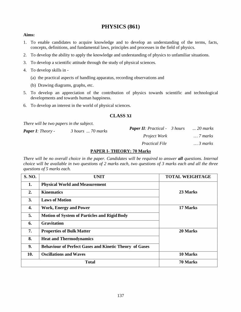
PHYSICS (861)

Aims:

1. To enable candidates to acquire knowledge and to develop an understanding of the terms, facts, concepts, definitions, and fundamental laws, principles and processes in the field of physics.

2. To develop the ability to apply the knowledge and understanding of physics to unfamiliar situations.

3. To develop a scientific attitude through the study of physical sciences.

4. To develop skills in -

(a) the practical aspects of handling apparatus, recording observations and

(b) Drawing diagrams, graphs, etc.

5. To develop an appreciation of the contribution of physics towards scientific and technological developments and towards human happiness.

6. To develop an interest in the world of physical sciences.

CLASS XI

There will be two papers in the subject.

Paper I: Theory - 3 hours ... 70 marks Paper II: Practical - 3 hours ... 20 marks

Project Work … 7 marks

Practical File … 3 marks

PAPER I- THEORY: 70 Marks

There will be no overall choice in the paper. Candidates will be required to answer all questions. Internal choice will be available in two questions of 2 marks each, two questions of 3 marks each and all the three questions of 5 marks each.

S. NO. UNIT TOTAL WEIGHTAGE

1. Physical World and Measurement

23 Marks 2. Kinematics

3. Laws of Motion

4. Work, Energy and Power 17 Marks

5. Motion of System of Particles and Rigid Body

6. Gravitation

7. Properties of Bulk Matter 20 Marks

8. Heat and Thermodynamics

9. Behaviour of Perfect Gases and Kinetic Theory of Gases

10. Oscillations and Waves 10 Marks

Total 70 Marks

138

PAPER I -THEORY – 70 MARKS

Note: (i) Unless otherwise specified, only S. I. Units are to be used while teaching and learning, as well as for answering questions.

(ii) All physical quantities to be defined as and when they are introduced along with their units and dimensions.

(iii) Numerical problems are included from all topics except where they are specifically excluded or where only qualitative treatment is required.

1. Physical World and Measurement

(i) Physical World:

Scope of Physics and its application in everyday life. Nature of physical laws.

Physics and its branches (only basic knowledge required); fundamental laws and fundamental forces in nature (gravitational force, electro-magnetic force, strong and weak nuclear forces; unification of forces). Application of Physics in technology and society (major scientists, their discoveries, inventions and laws/principles to be discussed briefly).

(ii) Units and Measurements

Measurement: need for measurement; units of measurement; systems of units: fundamental and derived units in SI; measurement of length, mass and time; accuracy and precision of measuring instruments; errors in measurement; significant figures.

Dimensional formulae of physical quantities and constants, dimensional analysis and its applications.

(a) Importance of measurement in scientific studies; physics is a science of measurement. Unit as a reference standard of measurement; essential properties. Systems of units; CGS, FPS, MKS, MKSA, and SI; the seven base units of SI selected by the General Conference of Weights and Measures in 1971 and their definitions, list of fundamental, supplementary and derived physical quantities; their units and symbols (strictly as per rule);

subunits and multiple units using prefixes for powers of 10 (from atto for 10-18 to tera for 1012); other common units such as fermi, angstrom (now outdated), light year, astronomical unit and parsec. A new unit of mass used in atomic physics is unified atomic mass unit with symbol u (not amu); rules for writing the names of units and their symbols in SI (upper case/lower case.) Derived units (with correct symbols); special names wherever applicable; expression in terms of base units (e.g.: N= kg m/s2).

(b) Accuracy of measurement, errors in measurement: precision of measuring instruments, instrumental errors, systematic errors, random errors and gross errors. Least count of an instrument and its implication on errors in measurements; absolute error, relative error and percentage error; combination of errors in (a) sum and difference, (b) product and quotient and (c) power of a measured quantity.

(c) Significant figures; their significance; rules for counting the number of significant figures; rules for (a) addition and subtraction, (b) multiplication/ division; ‘rounding off’ the uncertain digits; order of magnitude as statement of magnitudes in powers of 10; examples from magnitudes of common physical quantities - size, mass, time, etc.

(d) Dimensions of physical quantities; dimensional formula; express derived units in terms of base units (N = kg.m s-2); use symbol […] for dimensions of or base unit of; e.g.: dimensional formula of force in terms of fundamental quantities written as [F] = [MLT–2].Principle of homogeneity of dimensions. Expressions in terms of SI base units and dimensional formula may be obtained for all physical quantities as

139

and when new physical quantities are introduced.

(e) Use of dimensional analysis to (i) check the dimensional correctness of a formula/ equation; (ii) to obtain the dimensional formula of any derived physical quantity including constants; (iii) to convert units from one system to another; limitations of dimensional analysis.

2. Kinematics

(i) Motion in a Straight Line Frame of references, Motion in a straight line (one dimension): Position-time graph, speed and velocity. Elementary concepts of differentiation and integration for describing motion, uniform and non- uniform motion, average speed, velocity, average velocity, instantaneous velocity and uniformly accelerated motion, velocity - time and position - time graphs. Relations for uniformly accelerated motion (graphical treatment).

Frame of reference, concept of point mass, rest and motion; distance and displacement, speed and velocity, average speed and average velocity, uniform velocity, instantaneous speed and instantaneous velocity, acceleration, instantaneous acceleration, s-t, v-t and a-t graphs for uniform acceleration and conclusions drawn from these graphs; kinematic equations of motion for objects in uniformly accelerated rectilinear motion derived using graphical, calculus or analytical method, motion of an object under gravity, (one dimensional motion). Differentiation as rate of change; examples from physics – speed, acceleration, velocity gradient, etc. Formulae for differentiation of simple functions: xn, sinx, cosx, ex and ln x. Simple ideas about integration – mainly. ∫ xn.dx. Both definite and indefinite integrals to be mentioned (elementary calculus not to be evaluated).

(ii) Motion in a Plane Scalar and Vector quantities with examples. Position and displacement vectors, general vectors and their notations; equality of vectors, addition and subtraction of vectors, relative velocity, Unit vector; resolution of a vector in a plane, rectangular components, Scalar and Vector product of two vectors. Projectile motion and uniform circular motion.

(a) General Vectors and notation, position and displacement vector. Vectors explained using displacement as a prototype - along a straight line (one dimensional), on a plane surface (two dimensional) and in an open space not confined to a line or a plane (three dimensional); symbol and representation; a scalar quantity, its representation and unit, equality of vectors. Unit vectors denoted by i , j , k orthogonal unit vectors along x, y and z axes respectively. Examples of one dimensional vector

1V

=a i or b j or c k where a, b, c are

scalar quantities or numbers; 2V

= a i + b j is a two dimensional or

planar vector, 3V

= a i + b j + c k is a three dimensional or space vector. Concept of null vector and co-planar vectors.

(b) Addition: use displacement as an example; obtain triangle law of addition; graphical and analytical treatment; Discuss commutative and associative properties of vector addition (Proof not required). Parallelogram Law; sum and difference; derive expressions for magnitude and direction from parallelogram law; special cases; subtraction as special case of addition with direction reversed; use of Triangle Law for subtraction also; if a+ b

= c ; c - a= b

; In a parallelogram, if one diagonal is the

140

sum, the other diagonal is the difference; addition and subtraction with vectors expressed in terms of unit vectors i , j , k ; multiplication of a vector by a real number.

(c) Use triangle law of addition to express a vector in terms of its components. If a+ b

= c is an addition fact, c = a+ b

is a resolution; a and b

are components of c . Rectangular components, relation between components, resultant and angle between them. Dot (or scalar) product of vectors a . b

=abcosθ; example W = F

. S

= FS Cosθ . Special case of θ = 0o, 90 o and 1800. Vector (or cross) product a×b

= [absinθ] n ; example: torque τ= r × F

; Special cases using unit vectors i , j , k for

a . b

and a x b

. (d) Concept of relative velocity, start from

simple examples on relative velocity of one dimensional motion and then two dimensional motion; consider displacement first; relative displacement (use Triangle Law or parallelogram Law).

(e) Various terms related to projectile motion; obtain equations of trajectory, time of flight, maximum height, horizontal range, instantaneous velocity, [projectile motion on an inclined plane not included]. Examples of projectile motion.

(f) Examples of uniform circular motion: details to be covered in unit 3 (d).

3. Laws of Motion General concept of force, inertia, Newton's first law of motion; momentum and Newton's second law of motion; impulse; Newton's third law of motion. Law of conservation of linear momentum and its applications.

Equilibrium of concurrent forces. Friction: Static and kinetic friction, laws of friction, rolling friction, lubrication. Dynamics of uniform circular motion: Centripetal force, examples of circular motion (vehicle on a level circular road, vehicle on a banked road). (a) Newton's first law: Statement and

explanation; concept of inertia, mass, force; law of inertia; mathematically, if ∑F=0, a=0.

Newton's second law: p =m v ; F

α dpdt

;

F

=k dpdt

. Define unit of force so that

k=1; F

= dpdt

; a vector equation. For

classical physics with v not large and mass m remaining constant, obtain F

=m a . For v→ c, m is not constant. Then m =

22o

cv-1m Note that F= ma is the

special case for classical mechanics. It is a vector equation. a || F

. Also, this can be resolved into three scalar equations Fx=max etc. Application to numerical problems; introduce tension force, normal reaction force. If a = 0 (body in equilibrium), F= 0. Statement, derivation and explanation of principle of conservation of linear momentum. Impulse of a force: F∆t =∆p.

Newton's third law. Obtain it using Law of Conservation of linear momentum. Proof of Newton’s second law as real law. Systematic solution of problems in mechanics; isolate a part of a system, identify all forces acting on it; draw a free body diagram representing the part as a point and representing all forces by line segments, solve for resultant force which is equal to m a . Simple problems on “Connected bodies” (not involving two pulleys).

(b) Force diagrams; resultant or net force from Triangle law of Forces, parallelogram law or resolution of forces.

141

Apply net force ∑F

= m a . Again for equilibrium a=0 and ∑F=0. Conditions of equilibrium of a rigid body under three coplanar forces. Discuss ladder problem.

(c) Friction; classical view and modern view of friction, static friction a self-adjusting force; limiting value; kinetic friction or sliding friction; rolling friction, examples. Laws of friction: Two laws of static friction; (similar) two laws of kinetic friction; coefficient of friction µs = fs(max)/N and µk = fk/N; graphs. Friction as a non-conservative force; motion under friction, net force in Newton’s 2nd law is calculated including fk. Motion along a rough inclined plane – both up and down. Pulling and pushing of a roller. Angle of friction and angle of repose. Lubrication, use of bearings, streamlining, etc.

(d) Angular displacement (θ), angular velocity (ω), angular acceleration (α) and their relations. Concept of centripetal acceleration; obtain an expression for this acceleration using∆v

. Magnitude and direction of a same as that of ∆v

; Centripetal acceleration; the cause of this acceleration is a force - also called centripetal force; the name only indicates its direction, it is not a new type of force, motion in a vertical circle; banking of road and railway track (conical pendulum is excluded).

4. Work, Power and Energy

Work done by a constant force and a variable force; kinetic energy, work-energy theorem, power.

Potential energy, potential energy of a spring, conservative forces: conservation of mechanical energy (kinetic and potential energies); Conservative and non-conservative forces. Concept of collision: elastic and inelastic collisions in one and two dimensions. (i) Work done W= F

. S

=FScosθ. If F is variable dW= F

. dS

and W=∫dw= F∫

. dS

, for F

║ dS

F

. dS

=FdS

therefore, W=∫FdS is the area under the F-S graph or if F can be expressed in terms of S, ∫FdS can be evaluated. Example, work done in stretching a spring 21

2W Fdx kxdx kx= = =∫ ∫ . This

is also the potential energy stored in the stretched spring U=½ kx2

.

Kinetic energy and its expression, Work-Energy theorem E=W. Law of Conservation of Energy; oscillating spring. U+K = E = Kmax = Umax (for U = 0 and K = 0 respectively); graph different forms of energy and their transformations. E = mc2

(no derivation). Power P=W/t; .P F v=

.

(ii) Collision in one dimension; derivation of velocity equation for general case of m1 ≠ m2 and u1 ≠ u2=0; Special cases for m1=m2=m; m1>>m2 or m1<<m2. Oblique collisions i.e. collision in two dimensions.

5. Motion of System of Particles and Rigid Body

Idea of centre of mass: centre of mass of a two-particle system, momentum conservation and centre of mass motion. Centre of mass of a rigid body; centre of mass of a uniform rod.

Moment of a force, torque, angular momentum, laws of conservation of angular momentum and its applications.

Equilibrium of rigid bodies, rigid body rotation and equations of rotational motion, comparative study of linear and rotational motions.

Moment of inertia, radius of gyration, moments of inertia for simple geometrical objects (no derivation). Statement of parallel and perpendicular axes theorems and their applications.

(i) Definition of centre of mass (cm), centre of mass (cm) for a two particle system m1x1+m2x2=Mxcm; differentiating, get the equation for vcm and acm; general equation for N particles- many particles system; [need not go into more details];centre of gravity, principle of moment, discuss ladder problem, concept of a rigid body;

142

kinetic energy of a rigid body rotating about a fixed axis in terms of that of the particles of the body; hence, define moment of inertia and radius of gyration; physical significance of moment of inertia; unit and dimension; depends on mass and axis of rotation; it is rotational inertia; equations of rotational motions. Applications: only expression for the moment of inertia, I (about the symmetry axis) of: (i) a ring; (ii) a solid and a hollow cylinder, (iii) a thin rod (iv) a solid and a hollow sphere, (v) a disc - only formulae (no derivations required).

(a) Statements of the parallel and perpendicular axes theorems with illustrations [derivation not required]. Simple examples with change of axis.

(b) Definition of torque (vector); τ= r x F

and angular momentum L

= r x p for a particle (no derivations);

differentiate to obtain d L

/dt=τ ; similar to Newton’s second law of motion (linear);hence τ=I α and L = Iω; (only scalar equation); Law of conservation of angular momentum; simple applications. Comparison of linear and rotational motions.

6. Gravitation

Kepler's laws of planetary motion, universal law of gravitation. Acceleration due to gravity (g) and its variation with altitude, latitude and depth.

Gravitational potential and gravitational potential energy, escape velocity, orbital velocity of a satellite, Geo-stationary satellites.

(i) Newton's law of universal gravitation; Statement; unit and dimensional formula of universal gravitational constant, G [Cavendish experiment not required]; gravitational acceleration on surface of the earth (g), weight of a body W= mg from F=ma.

(ii) Relation between g and G. Derive the expression for variation of g above and below the surface of the earth; graph; mention variation of g with latitude and rotation, (without derivation).

(iii) Gravitational field, intensity of gravitational field and potential at a point in earth’s gravitational field. Vp = Wαp/m. Derive expression (by integration) for the gravitational potential difference ∆V = VB-VA = G.M(1/rA-1/rB); here Vp = V(r) = -GM/r; negative sign for attractive force field; define gravitational potential energy of a mass m in the earth's field; expression for gravitational potential energy U(r) = Wαp = m.V(r) = -G M m/r; show that ∆U = mgh, for h << R. Relation between intensity and acceleration due to gravity.

(iv) Derive expression for the escape velocity of earth using energy consideration; ve depends on mass of the earth; for moon ve is less as mass of moon is less; consequence - no atmosphere on the moon.

(v) Satellites (both natural (moon) and artificial) in uniform circular motion around the earth; Derive the expression for orbital velocity and time period; note the centripetal acceleration is caused (or centripetal force is provided) by the force of gravity exerted by the earth on the satellite; the acceleration of the satellite is the acceleration due to gravity [g’= g(R/R+h)2; F’G = mg’]. Weightlessness; geostationary satellites; conditions for satellite to be geostationary; parking orbit, calculation of its radius and height; basic concept of polar satellites and their uses.

(vi) Kepler's laws of planetary motion: explain the three laws using diagrams. Proof of third law (for circular orbits only).

7. Properties of Bulk Matter (i) Mechanical Properties of Solids: Elastic

behaviour of solids, Stress-strain relationship, Hooke's law, Young's modulus, bulk modulus, shear modulus

143

of rigidity, Poisson's ratio; elastic energy.

Elasticity in solids, Hooke’s law, Young modulus and its determination, bulk modulus and shear modulus of rigidity, work done in stretching a wire and strain energy, Poisson’s ratio.

(ii) Mechanical Properties of Fluids

Pressure due to a fluid column; Pascal's law and its applications (hydraulic lift and hydraulic brakes), effect of gravity on fluid pressure.

Viscosity, Stokes' law, terminal velocity, streamline and turbulent flow, critical velocity, Bernoulli's theorem and its applications.

Surface energy and surface tension, angle of contact, excess of pressure across a curved surface, application of surface tension ideas to drops, bubbles and capillary rise.

(a) Pressure in a fluid, Pascal’s Law and its applications, buoyancy (Archimedes Principle).

(b) General characteristics of fluid flow; equation of continuity v1a1= v2a2; conditions; applications like use of nozzle at the end of a hose; Bernoulli’s principle (theorem); assumptions - incompressible liquid, streamline (steady) flow, non-viscous and irrotational liquid - ideal liquid; derivation of equation; applications of Bernoulli’s theorem atomizer, dynamic uplift, Venturimeter, Magnus effect etc.

(c) Streamline and turbulent flow - examples; streamlines do not intersect (like electric and magnetic lines of force); tubes of flow; number of streamlines per unit area α velocity of flow (from equation of continuity v1a1 = v2a2); critical velocity; Reynold's number (significance only) Poiseuille’s formula with numericals.

(d) Viscous drag; Newton's formula for viscosity, co-efficient of viscosity and its units.

Flow of fluids (liquids and gases), laminar flow, internal friction between layers of fluid, between fluid and the solid with which the fluid is in relative motion; examples; viscous drag is a force of friction; mobile and viscous liquids.

Velocity gradient dv/dx (space rate of change of velocity); viscous drag F = ηA dv/dx; coefficient of viscosity η = F/A (dv/dx) depends on the nature of the liquid and its temperature; units: Ns/m2 and dyn.s/cm2= poise.1 poise=0.1 Ns/m2.

(e) Stoke's law, motion of a sphere falling through a fluid, hollow rigid sphere rising to the surface of a liquid, parachute, obtain the expression of terminal velocity; forces acting; viscous drag, a force proportional to velocity; Stoke’s law; ν-t graph.

(f) Surface tension (molecular theory), drops and bubbles, angle of contact, work done in stretching a surface and surface energy, capillary rise, measurement of surface tension by capillary (uniform bore) rise method. Excess pressure across a curved surface, application of surface tension for drops and bubbles.

8. Heat and Thermodynamics

(i) Thermal Properties of Matter: Heat, temperature, thermal expansion; thermal expansion of solids, liquids and gases, anomalous expansion of water; specific heat capacity, calorimetry; change of state, specific latent heat capacity.

Heat transfer-conduction, convection and radiation, thermal conductivity, qualitative ideas of Blackbody radiation, Wein's displacement Law, Stefan's law, and Greenhouse effect.

144

(a) Temperature and Heat, measurement of temperature (scales and inter conversion). Ideal gas equation and absolute temperature, thermal expansion in solids, liquids and gases. Specific heat capacity, calorimetry, change of state, latent heat capacity, steady state and temperature gradient. Thermal conductivity; co-efficient of thermal conductivity, Use of good and poor conductors, Searle’s experiment,(Lee’s Disc method is not required). Convection with examples.

(b) Black body is now called ideal or cavity radiator and black body radiation is cavity radiation; Stefan’s law is now known as Stefan Boltzmann law as Boltzmann derived it theoretically. There is multiplicity of technical terms related to thermal radiation - radiant intensity I (T) for total radiant power (energy radiated/second) per unit area of the surface, in W/m2, I (T) =σ T4; dimension and SI unit of σ. For practical radiators I =∈. σ T4 where ∈ (dimension less) is called emissivity of the surface material; ∈=1 for ideal radiators. The Spectral radiancy R(λ). I (T)=

0R

α

∫ (λ) dλ.

Graph of R(λ) vs λ for different temperatures. Area under the graph is I (T). The λ corresponding to maximum value of R is called λmax; decreases with increase in temperature.

Wien’s displacement law; Stefan’s law and Newton’s law of cooling. [Deductions from Stefan’s law not necessary]. Greenhouse effect – self-explanatory.

(ii) Thermodynamics

Thermal equilibrium and definition of temperature (zeroth law of thermodynamics), heat, work and internal energy. First law of thermodynamics, isothermal and adiabatic processes.

Second law of thermodynamics: reversible and irreversible processes, Heat engine and refrigerator.

(a) Thermal equilibrium and zeroth law of thermodynamics: Self explanatory

(b) First law of thermodynamics.

Concept of heat (Q) as the energy that is transferred (due to temperature difference only) and not stored; the energy that is stored in a body or system as potential and kinetic energy is called internal energy (U). Internal energy is a state property (only elementary ideas) whereas, heat is not; first law is a statement of conservation of energy, when, in general, heat (Q) is transferred to a body (system), internal energy (U) of the system changes and some work W is done by the system; then Q=∆U+W; also W=∫pdV for working substance - an ideal gas; explain the meaning of symbols (with examples) and sign convention carefully (as used in physics: Q>0 when added to a system, ∆U>0 when U increases or temperature rises, and W>0 when work is done by the system). Special cases for Q=0 (adiabatic), ∆U=0 (isothermal) and W=0 (isochoric).

(c) Isothermal and adiabatic changes in a perfect gas described in terms of PV graphs; PV = constant (Isothermal) and PVγ = constant (adiabatic); joule and calorie relation (derivation of PVγ = constant not required).

Note that 1 cal = 4⋅186 J exactly and J (so-called mechanical equivalent of heat) should not be used in equations. In equations, it is understood that each term as well as the LHS and RHS are in the same units; it could be all joules or all calories.

(d) Derive an expression for work done in isothermal and adiabatic processes; principal and molar heat capacities; Cp and Cv; relation between Cp and

145

Cv (Cp - Cv = R). Work done as area bounded by PV graph.

(e) Second law of thermodynamics, Carnot's cycle. Some practical applications.

Only one statement each in terms of Kelvin’s impossible steam engine and Clausius’ impossible refrigerator. Brief explanation of the law. Reversible and irreversible processes, Heat engine; Carnot’s cycle - describe realisation from source and sink of infinite thermal capacity, thermal insulation, etc. Explain using pV graph (isothermal process and adiabatic process) expression and numericals (without derivation) for efficiency η=1-T2/T1., Refrigerator and heat pumps.

9. Behaviour of Perfect Gases and Kinetic Theory of Gases

(i) Kinetic Theory: Equation of state of a perfect gas, work done in compressing a gas. Kinetic theory of gases - assumptions, concept of pressure. Kinetic interpretation of temperature; rms speed of gas molecules; degrees of freedom, law of equi-partition of energy (statement only) and application to specific heat capacities of gases; concept of mean free path, Avogadro's number.

(a) Kinetic Theory of gases; derive p=1/3 ρ 2c from the assumptions and applying Newton’s laws of motion. The average thermal velocity (rms value) crms=√3p/ρ; calculations for air, hydrogen and their comparison with common speeds. Effect of temperature and pressure on rms speed of gas molecules.

[Note that pV=nRT the ideal gas equation cannot be derived from kinetic theory of ideal gas. Hence, neither can other gas laws; pV=nRT is an experimental result. Comparing this with p = ⅓ ρ 2c , from kinetic theory of gases, a kinetic interpretation

of temperature can be obtained as explained in the next subunit].

(b) From kinetic theory for an ideal gas (obeying all the assumptions especially no intermolecular attraction and negligibly small size of molecules, we get p = (1/3)ρ 2c or pV =

(1/3)M 2c . (No further, as temperature is not a concept of kinetic theory). From experimentally obtained gas laws, we have the ideal gas equation (obeyed by some gases at low pressure and high temperature) pV = RT for one mole. Combining these two results (assuming they can be combined), RT=(1/3)M 2c =(2/3).½M 2c =(2/3)K; Hence, kinetic energy of 1 mole of an ideal gas K=(3/2)RT. Average K for 1 molecule = K/N = (3/2) RT/N = (3/2) kT where k is Boltzmann’s constant. So, temperature T can be interpreted as a measure of the average kinetic energy of the molecules of a gas.

(c) Degrees of freedom and calculation of specific heat capacities for all types of gases. Concept of the law of equipartition of energy (derivation not required). Concept of mean free path and Avogadro’s number NA.

10. Oscillations and Waves

(i) Oscillations: Periodic motion, time period, frequency, displacement as a function of time, periodic functions. Simple harmonic motion (S.H.M) and its equation; phase; oscillations of a spring, restoring force and force constant; energy in S.H.M., Kinetic and potential energies; simple pendulum and derivation of expression for its time period.

Free, forced and damped oscillations (qualitative ideas only), resonance.

(a) Simple harmonic motion. Periodic motion, time period T and frequency f, f=1/T; uniform circular motion and its projection on a diameter defines SHM; displacement, amplitude, phase and epoch, velocity, acceleration, time

146

period; characteristics of SHM; Relation between linear simple harmonic motion and uniform circular motion. Differential equation of SHM, d2y/dt2+ω2y=0 from the nature of force acting F=-k y; solution y=A sin (ωt+φ0) where ω2 = k/m; obtain expressions for velocity, acceleration, time period T and frequency f. Graphical representation of displacement, velocity and acceleration. Examples, simple pendulum, a mass m attached to a spring of spring constant k. Derivation of time period of simple harmonic motion of a simple pendulum, mass on a spring (horizontal and vertical oscillations) Kinetic and potential energy at a point in simple harmonic motion. Total energy E = U+K (potential +kinetic) is conserved. Draw graphs of U, K and E Verses y.

(b) Free, forced and damped oscillations (qualitative treatment only). Resonance. Examples of damped oscillations (all oscillations are damped); graph of amplitude vs time for undamped and damped oscillations; damping force in addition to restoring force (-ky); forced oscillations, examples; action of an external periodic force, in addition to restoring force. Time period is changed to that of the external applied force, amplitude (A) varies with frequency (f) of the applied force and it is maximum when the frequency of the external applied force is equal to the natural frequency of the vibrating body. This is resonance; maximum energy transfer from one body to the other; bell graph of amplitude vs frequency of the applied force. Examples from mechanics, electricity and electronics (radio).

(ii) Waves: Wave motion, Transverse and longitudinal waves, speed of wave motion, displacement relation for a progressive wave, principle of superposition of waves, reflection of waves, standing waves in

strings and organ pipes, fundamental mode and harmonics, Beats, Doppler effect.

(a) Transverse and longitudinal waves; characteristics of a harmonic wave; graphical representation of a harmonic wave. Distinction between transverse and longitudinal waves; examples; displacement, amplitude, time period, frequency, wavelength, derive v=fλ; graph of displacement with time/position, label time period/wavelength and amplitude, equation of a progressive harmonic (sinusoidal) wave, y = A sin (kx±ωt) where k is a propagation factor and equivalent equations.

(b) Production and propagation of sound as a wave motion; mechanical wave requires a medium; general formula for speed of sound (no derivation). Newton’s formula for speed of sound in air; experimental value; Laplace’s correction; variation of speed v with changes in pressure, density, humidity and temperature. Speed of sound in liquids and solids - brief introduction only. Concept of supersonic and ultrasonic waves.

(c) Principle of superposition of waves; interference (simple ideas only); dependence of combined wave form, on the relative phase of the interfering waves; qualitative only - illustrate with wave representations. Beats (qualitative explanation only); number of beats produced per second = difference in the frequencies of the interfering waves. Standing waves or stationary waves; formation by two identical progressive waves travelling in opposite directions (e.g.,: along a string, in an air column - incident and reflected waves); obtain y= y1+y2= [2 ym sin (kx)] cos (ωt) using equations of the travelling waves; variation of the amplitude A=2 ymsin (kx) with location (x) of the particle; nodes and antinodes; compare

147

standing waves with progressive waves.

(d) Laws of vibrations of a stretched string. Obtain equation for fundamental frequency f0=(½l) T/m ; sonometer.

(e) Modes of vibration of strings and air columns (closed and open pipes); standing waves with nodes and antinodes; also in resonance with the periodic force exerted usually by a tuning fork; sketches of various modes of vibration; obtain expressions for fundamental frequency and various harmonics and overtones; mutual relations.

(f) Doppler effect for sound; obtain general expression for apparent frequency when both the source and listener are moving,

given as LL r

r

v vf fv v

±= ±

which can be

reduced to any one of the four special cases, by using proper sign.

PAPER II

PRACTICAL WORK- 20 Marks

Given below is a list of required experiments. Teachers may add to this list, keeping in mind the general pattern of questions asked in the annual examinations.

In each experiment, students are expected to record their observations in a tabular form with units at the column head. Students should plot an appropriate graph, work out the necessary calculations and arrive at the result.

Students are required to have completed all experiments from the given list (excluding demonstration experiments):

1. To measure the diameter of a spherical body using Vernier calipers. Calculate its volume with appropriate significant figures. Also measure its volume using a graduated cylinder and compare the two.

2. Find the diameter of a wire using a micrometer screw gauge and determine percentage error in cross sectional area.

3. Determine radius of curvature of a spherical surface like watch glass by a spherometer.

4. Equilibrium of three concurrent coplanar forces. To verify the parallelogram law of forces and to determine weight of a body.

5. (i) Inclined plane: To find the downward force acting along the inclined plane on a roller due to gravitational pull of earth and to study its relationship with angle of inclination by plotting graph between force and sin θ.

(ii) Friction: To find the force of limiting friction for a wooden block placed on horizontal surface and to study its relationship with normal reaction. To determine the coefficient of friction.

6. To find the acceleration due to gravity by measuring the variation in time period (T) with effective length (L) of a simple pendulum; plot graphs of T νs √L and T2 νs L. Determine effective length of the seconds pendulum from T2 νs L graph.

7. To find the force constant of a spring and to study variation in time period of oscillation with mass m of a body suspended by the spring. To find acceleration due to gravity by plotting a graph of T against √m.

8. Boyle's Law: To study the variation in volume with pressure for a sample of air at constant temperature by plotting graphs between p and

V1 and between p and V.

9. Cooling curve: To study the fall in temperature of a body (like hot water or liquid in calorimeter) with time. Find the slope of the curve at four different temperatures of the hot body and hence, deduce Newton's law of cooling.

10. To study the variation in frequency of air column with length using resonance column apparatus or a long cylindrical vessel and a set of tuning forks. Hence, determine velocity of sound in air at room temperature.

11. To determine frequency of a tuning fork using a sonometer.

12. To determine specific heat capacity of a solid using a calorimeter.

148

Demonstration Experiments (The following experiments are to be demonstrated by the teacher):

1. Searle's method to determine Young modulus of elasticity.

2. Capillary rise method to determine surface tension of water.

3. Determination of coefficient of viscosity of a given viscous liquid by terminal velocity method.

PROJECT WORK AND PRACTICAL FILE –

10 Marks Project Work – 7 Marks All candidates will be required to do one project involving some Physics related topic/s, under the guidance and regular supervision of the Physics teacher. Candidates are to prepare a technical report formally written including an abstract, some theoretical discussion, experimental setup, observations with tables of data collected, analysis and discussion of results, deductions, conclusion, etc. (after the draft has been approved by the teacher). The report should be kept simple, but neat and elegant. No extra credit shall be given for type-written material/decorative cover, etc. Teachers may assign or students may choose any one project of their choice.

Suggested Evaluation criteria:

Title and Abstract (summary)

Introduction / purpose

Contents/Presentation

Analysis/ material aid (graph, data, structure, pie charts, histograms, diagrams, etc.)

Originality of work

Conclusion/comments

Practical File – 3 Marks

Teachers are required to assess students on the basis of the Physics practical file maintained by them during the academic year.

NOTE: For guidelines regarding Project Work, please refer to Class XII.

149

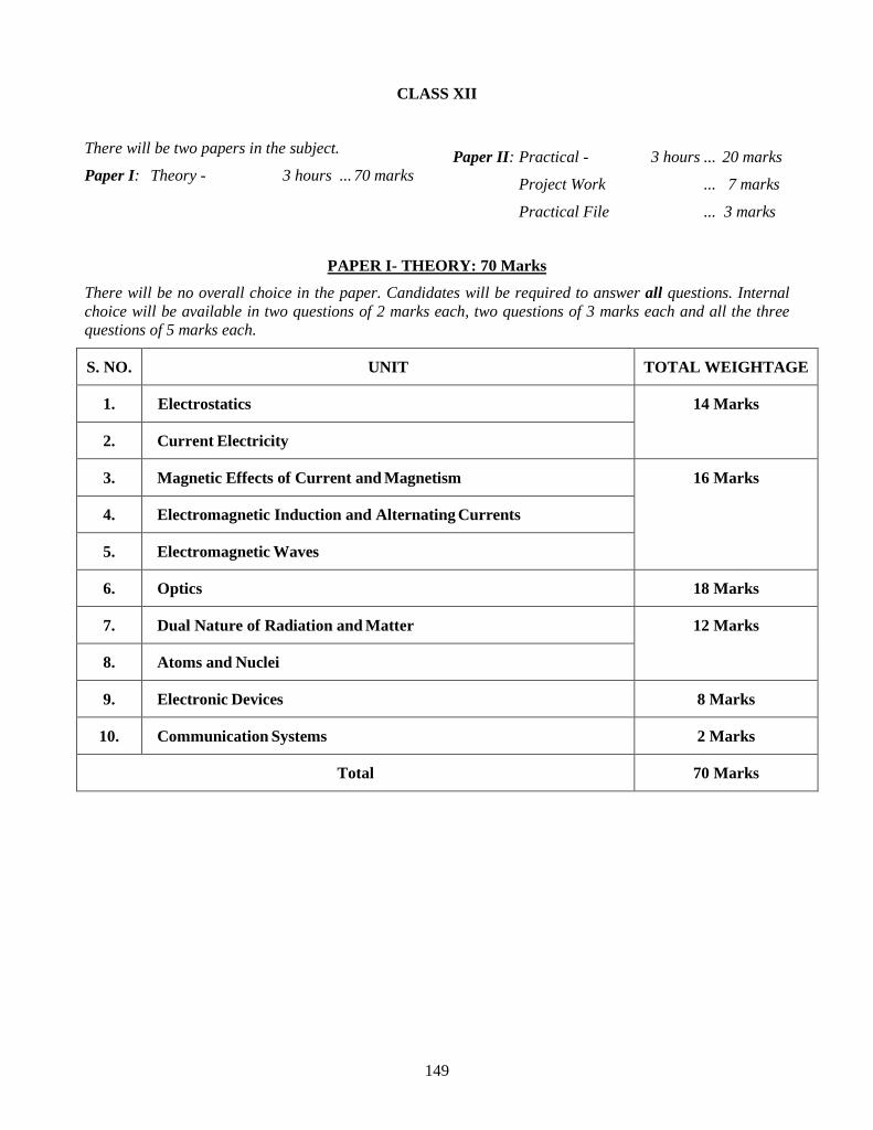
CLASS XII

There will be two papers in the subject.

Paper I: Theory - 3 hours ... 70 marks Paper II: Practical - 3 hours ... 20 marks

Project Work ... 7 marks

Practical File ... 3 marks

PAPER I- THEORY: 70 Marks

There will be no overall choice in the paper. Candidates will be required to answer all questions. Internal choice will be available in two questions of 2 marks each, two questions of 3 marks each and all the three questions of 5 marks each.

S. NO. UNIT TOTAL WEIGHTAGE

1. Electrostatics 14 Marks

2. Current Electricity

3. Magnetic Effects of Current and Magnetism 16 Marks

4. Electromagnetic Induction and Alternating Currents

5. Electromagnetic Waves

6. Optics 18 Marks

7. Dual Nature of Radiation and Matter 12 Marks

8. Atoms and Nuclei

9. Electronic Devices 8 Marks

10. Communication Systems 2 Marks

Total 70 Marks

150

PAPER I -THEORY- 70 Marks

Note: (i) Unless otherwise specified, only S. I. Units are to be used while teaching and learning, as well as for answering questions.

(ii) All physical quantities to be defined as and when they are introduced along with their units and dimensions.

(iii) Numerical problems are included from all topics except where they are specifically excluded or where only qualitative treatment is required.

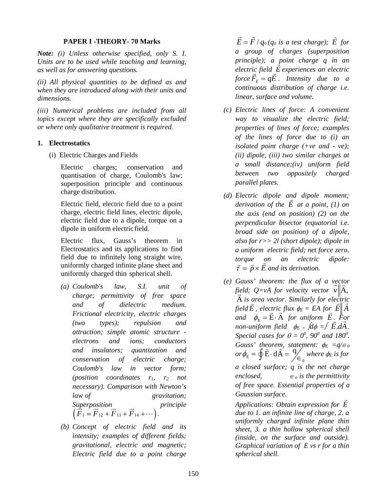
1. Electrostatics

(i) Electric Charges and Fields

Electric charges; conservation and quantisation of charge, Coulomb's law; superposition principle and continuous charge distribution.

Electric field, electric field due to a point charge, electric field lines, electric dipole, electric field due to a dipole, torque on a dipole in uniform electric field.

Electric flux, Gauss’s theorem in Electrostatics and its applications to find field due to infinitely long straight wire, uniformly charged infinite plane sheet and uniformly charged thin spherical shell.

(a) Coulomb's law, S.I. unit of charge; permittivity of free space and of dielectric medium. Frictional electricity, electric charges (two types); repulsion and attraction; simple atomic structure - electrons and ions; conductors and insulators; quantization and conservation of electric charge; Coulomb's law in vector form; (position coordinates r1, r2 not necessary). Comparison with Newton’s law of gravitation; Superposition principle ( )1 12 13 14F F F F= + + + ⋅⋅⋅

.

(b) Concept of electric field and its intensity; examples of different fields; gravitational, electric and magnetic; Electric field due to a point charge

/ oE F q=

(q0 is a test charge); E

for a group of charges (superposition principle); a point charge q in an electric field E

experiences an electric force EF qE=

. Intensity due to a continuous distribution of charge i.e. linear, surface and volume.

(c) Electric lines of force: A convenient way to visualize the electric field; properties of lines of force; examples of the lines of force due to (i) an isolated point charge (+ve and - ve); (ii) dipole, (iii) two similar charges at a small distance;(iv) uniform field between two oppositely charged parallel plates.

(d) Electric dipole and dipole moment; derivation of the E

at a point, (1) on the axis (end on position) (2) on the perpendicular bisector (equatorial i.e. broad side on position) of a dipole, also for r>> 2l (short dipole); dipole in a uniform electric field; net force zero, torque on an electric dipole:

p Eτ = ×

and its derivation.

(e) Gauss’ theorem: the flux of a vector field; Q=vA for velocity vector A,v

A

is area vector. Similarly for electric field E

, electric flux φE = EA for E A

and E E Aφ = ⋅

for uniform E

. For non-uniform field φE = ∫dφ =∫ .E dA

. Special cases for θ = 00, 900 and 1800. Gauss’ theorem, statement: φE =q/∈0

or Eφ =0

qE dA⋅ = ∈∫

where φE is for

a closed surface; q is the net charge enclosed, ∈o is the permittivity of free space. Essential properties of a Gaussian surface. Applications: Obtain expression for E

due to 1. an infinite line of charge, 2. a uniformly charged infinite plane thin sheet, 3. a thin hollow spherical shell (inside, on the surface and outside). Graphical variation of E vs r for a thin spherical shell.

151

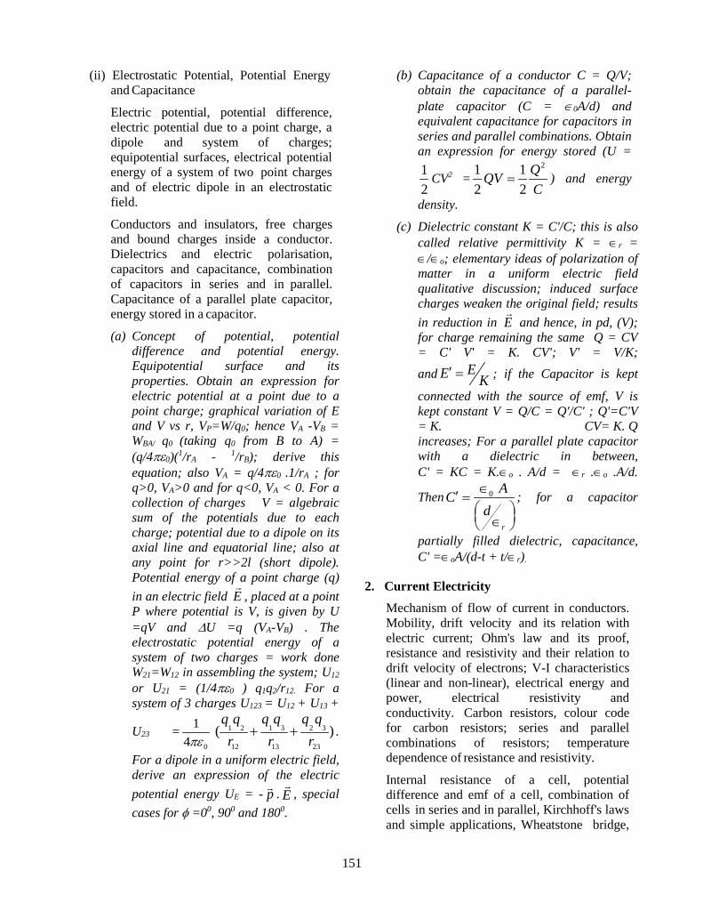
(ii) Electrostatic Potential, Potential Energy and Capacitance

Electric potential, potential difference, electric potential due to a point charge, a dipole and system of charges; equipotential surfaces, electrical potential energy of a system of two point charges and of electric dipole in an electrostatic field.

Conductors and insulators, free charges and bound charges inside a conductor. Dielectrics and electric polarisation, capacitors and capacitance, combination of capacitors in series and in parallel. Capacitance of a parallel plate capacitor, energy stored in a capacitor.

(a) Concept of potential, potential difference and potential energy. Equipotential surface and its properties. Obtain an expression for electric potential at a point due to a point charge; graphical variation of E and V vs r, VP=W/q0; hence VA -VB = WBA/ q0 (taking q0 from B to A) = (q/4πε0)(1/rA - 1/rB); derive this equation; also VA = q/4πε0 .1/rA ; for q>0, VA>0 and for q<0, VA < 0. For a collection of charges V = algebraic sum of the potentials due to each charge; potential due to a dipole on its axial line and equatorial line; also at any point for r>>2l (short dipole). Potential energy of a point charge (q) in an electric field E

, placed at a point P where potential is V, is given by U =qV and ∆U =q (VA-VB) . The electrostatic potential energy of a system of two charges = work done W21=W12 in assembling the system; U12 or U21 = (1/4πε0 ) q1q2/r12. For a system of 3 charges U123 = U12 + U13 +

U23 =0

14πε

1 3 2 31 2

12 13 23

( )q q q qq q

r r r+ + .

For a dipole in a uniform electric field, derive an expression of the electric potential energy UE = - p . E

, special cases for φ =00, 900 and 1800.

(b) Capacitance of a conductor C = Q/V; obtain the capacitance of a parallel-plate capacitor (C = ∈0A/d) and equivalent capacitance for capacitors in series and parallel combinations. Obtain an expression for energy stored (U = 12

CV2 =21 1

2 2QQVC

= ) and energy

density.

(c) Dielectric constant K = C'/C; this is also called relative permittivity K = ∈r = ∈/∈o; elementary ideas of polarization of matter in a uniform electric field qualitative discussion; induced surface charges weaken the original field; results in reduction in E

and hence, in pd, (V); for charge remaining the same Q = CV = C' V' = K. CV'; V' = V/K; and EE K′ = ; if the Capacitor is kept

connected with the source of emf, V is kept constant V = Q/C = Q'/C' ; Q'=C'V = K. CV= K. Q increases; For a parallel plate capacitor with a dielectric in between, C' = KC = K.∈o . A/d = ∈r .∈o .A/d.

Then 0

r

ACd∈′ = ∈

; for a capacitor

partially filled dielectric, capacitance, C' =∈oA/(d-t + t/∈r).

2. Current Electricity

Mechanism of flow of current in conductors. Mobility, drift velocity and its relation with electric current; Ohm's law and its proof, resistance and resistivity and their relation to drift velocity of electrons; V-I characteristics (linear and non-linear), electrical energy and power, electrical resistivity and conductivity. Carbon resistors, colour code for carbon resistors; series and parallel combinations of resistors; temperature dependence of resistance and resistivity.

Internal resistance of a cell, potential difference and emf of a cell, combination of cells in series and in parallel, Kirchhoff's laws and simple applications, Wheatstone bridge,

152

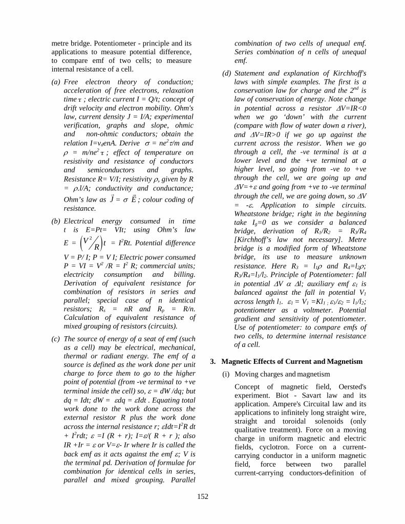
metre bridge. Potentiometer - principle and its applications to measure potential difference, to compare emf of two cells; to measure internal resistance of a cell.

(a) Free electron theory of conduction; acceleration of free electrons, relaxation timeτ ; electric current I = Q/t; concept of drift velocity and electron mobility. Ohm's law, current density J = I/A; experimental verification, graphs and slope, ohmic and non-ohmic conductors; obtain the relation I=vdenA. Derive σ = ne2τ/m and ρ = m/ne2τ ; effect of temperature on resistivity and resistance of conductors and semiconductors and graphs. Resistance R= V/I; resistivity ρ, given by R = ρ.l/A; conductivity and conductance; Ohm’s law as J

= σ E

; colour coding of resistance.

(b) Electrical energy consumed in time t is E=Pt= VIt; using Ohm’s law

E = ( )2V tR = I2Rt. Potential difference

V = P/ I; P = V I; Electric power consumed P = VI = V2 /R = I2 R; commercial units; electricity consumption and billing. Derivation of equivalent resistance for combination of resistors in series and parallel; special case of n identical resistors; Rs = nR and Rp = R/n. Calculation of equivalent resistance of mixed grouping of resistors (circuits).

(c) The source of energy of a seat of emf (such as a cell) may be electrical, mechanical, thermal or radiant energy. The emf of a source is defined as the work done per unit charge to force them to go to the higher point of potential (from -ve terminal to +ve terminal inside the cell) so, ε = dW /dq; but dq = Idt; dW = εdq = εIdt . Equating total work done to the work done across the external resistor R plus the work done across the internal resistance r; εIdt=I2R dt + I2rdt; ε =I (R + r); I=ε/( R + r ); also IR +Ir = ε or V=ε- Ir where Ir is called the back emf as it acts against the emf ε; V is the terminal pd. Derivation of formulae for combination for identical cells in series, parallel and mixed grouping. Parallel

combination of two cells of unequal emf. Series combination of n cells of unequal emf.

(d) Statement and explanation of Kirchhoff's laws with simple examples. The first is a conservation law for charge and the 2nd is law of conservation of energy. Note change in potential across a resistor ∆V=IR<0 when we go ‘down’ with the current (compare with flow of water down a river), and ∆V=IR>0 if we go up against the current across the resistor. When we go through a cell, the -ve terminal is at a lower level and the +ve terminal at a higher level, so going from -ve to +ve through the cell, we are going up and ∆V=+ε and going from +ve to -ve terminal through the cell, we are going down, so ∆V = -ε. Application to simple circuits. Wheatstone bridge; right in the beginning take Ig=0 as we consider a balanced bridge, derivation of R1/R2 = R3/R4

[Kirchhoff’s law not necessary]. Metre bridge is a modified form of Wheatstone bridge, its use to measure unknown resistance. Here R3 = l1ρ and R4=l2ρ; R3/R4=l1/l2. Principle of Potentiometer: fall in potential ∆V α ∆l; auxiliary emf ε1 is balanced against the fall in potential V1 across length l1. ε1 = V1 =Kl1 ; ε1/ε2 = l1/l2; potentiometer as a voltmeter. Potential gradient and sensitivity of potentiometer. Use of potentiometer: to compare emfs of two cells, to determine internal resistance of a cell.

3. Magnetic Effects of Current and Magnetism

(i) Moving charges and magnetism

Concept of magnetic field, Oersted's experiment. Biot - Savart law and its application. Ampere's Circuital law and its applications to infinitely long straight wire, straight and toroidal solenoids (only qualitative treatment). Force on a moving charge in uniform magnetic and electric fields, cyclotron. Force on a current-carrying conductor in a uniform magnetic field, force between two parallel current-carrying conductors-definition of

153

ampere, torque experienced by a current loop in uniform magnetic field; moving coil galvanometer - its sensitivity. Conversion of galvanometer into an ammeter and a voltmeter.

(ii) Magnetism and Matter:

A current loop as a magnetic dipole, its magnetic dipole moment, magnetic dipole moment of a revolving electron, magnetic field intensity due to a magnetic dipole (bar magnet) on the axial line and equatorial line, torque on a magnetic dipole (bar magnet) in a uniform magnetic field; bar magnet as an equivalent solenoid, magnetic field lines; earth's magnetic field and magnetic elements. Diamagnetic, paramagnetic, and ferromagnetic substances, with examples. Electromagnets and factors affecting their strengths, permanent magnets.

(a) Only historical introduction through Oersted’s experiment. [Ampere’s swimming rule not included]. Biot-Savart law and its vector form; application; derive the expression for B (i) at the centre of a circular loop carrying current; (ii) at any point on its axis. Current carrying loop as a magnetic dipole. Ampere’s Circuital law: statement and brief explanation. Apply it to obtain B

near a long wire carrying current and for a solenoid (straight as well as torroidal). Only formula of B

due to a finitely long conductor.

(b) Force on a moving charged particle in magnetic field ( )BF q v B= ×

; special

cases, modify this equation substituting dtld / for v and I for q/dt to yield F

= I dl ×

B

for the force acting on a current carrying conductor placed in a magnetic field. Derive the expression for force between two long and parallel wires carrying current, hence, define ampere (the base SI unit of current) and hence, coulomb; from Q = It. Lorentz force, Simple ideas about

principle, working, and limitations of a cyclotron.

(c) Derive the expression for torque on a current carrying loop placed in a uniform B

, using F

= I l B×

and τ

= r F×

; τ = NIAB sinφ for N turns τ

= m

× B

, where the dipole moment m

= NI A

, unit: A.m2. A current carrying loop is a magnetic dipole; directions of current and B

and m using right hand rule only; no other rule necessary. Mention orbital magnetic moment of an electron in Bohr model of H atom. Concept of radial magnetic field. Moving coil galvanometer; construction, principle, working, theory I= kφ , current and voltage sensitivity. Shunt. Conversion of galvanometer into ammeter and voltmeter of given range.

(d) Magnetic field represented by the symbol B is now defined by the equation ( ) o v BF q ×=

; B

is not to be defined in terms of force acting on a unit pole, etc.; note the distinction of B

from E

is that B

forms closed loops as there are no magnetic monopoles, whereas E

lines start from +ve charge and end on -ve charge. Magnetic field lines due to a magnetic dipole (bar magnet). Magnetic field in end-on and broadside-on positions (No derivations). Magnetic flux φ = B

. A

= BA for B uniform and B

A

; i.e. area held perpendicular to For φ = BA( B

A

), B=φ/A is the flux density [SI unit of flux is weber (Wb)]; but note that this is not correct as a defining equation as B

is vector and φ and φ/A are scalars, unit of B is tesla (T) equal to 10-4 gauss. For non-uniform B

field, φ = ∫dφ=∫ B

. dA

. Earth's magnetic field B

E is uniform over a limited area like that of a lab; the component of this

154

field in the horizontal direction BH is the one effectively acting on a magnet suspended or pivoted horizontally. Elements of earth’s magnetic field, i.e. BH, δ and θ - their definitions and relations.

(e) Properties of diamagnetic, paramagnetic and ferromagnetic substances; their susceptibility and relative permeability.

It is better to explain the main distinction, the cause of magnetization (M) is due to magnetic dipole moment (m) of atoms, ions or molecules being 0 for dia, >0 but very small for para and > 0 and large for ferromagnetic materials; few examples; placed in external B

, very small (induced) magnetization in a direction opposite to B

in dia, small magnetization parallel to B

for para, and large magnetization parallel to B

for ferromagnetic materials; this leads to lines of B

becoming less dense, more dense and much more dense in dia, para and ferro, respectively; hence, a weak repulsion for dia, weak attraction for para and strong attraction for ferro magnetic material. Also, a small bar suspended in the horizontal plane becomes perpendicular to the B

field for dia and parallel to B

for para and ferro. Defining equation H = (B/µ0)-M; the magnetic properties, susceptibility χm = (M/H) < 0 for dia (as M is opposite H) and >0 for para, both very small, but very large for ferro; hence relative permeability µr =(1+ χm) < 1 for dia, > 1 for para and >>1 (very large) for ferro; further, χm∝1/T (Curie’s law) for para, independent of temperature (T) for dia and depends on T in a complicated manner for ferro; on heating ferro becomes para at Curie temperature. Electromagnet: its definition, properties and factors affecting the strength of electromagnet; selection of magnetic material for

temporary and permanent magnets and core of the transformer on the basis of retentivity and coercive force (B-H loop and its significance, retentivity and coercive force not to be evaluated).

4. Electromagnetic Induction and Alternating Currents

(i) Electromagnetic Induction Faraday's laws, induced emf and current; Lenz's Law, eddy currents. Self-induction and mutual induction. Transformer.

(ii) Alternating Current Peak value, mean value and RMS value of alternating current/voltage; their relation in sinusoidal case; reactance and impedance; LC oscillations (qualitative treatment only), LCR series circuit, resonance; power in AC circuits, wattless current. AC generator. (a) Electromagnetic induction, Magnetic

flux, change in flux, rate of change of flux and induced emf; Faraday’s laws. Lenz's law, conservation of energy; motional emf ε = Blv, and power P = (Blv)2/R; eddy currents (qualitative);

(b) Self-Induction, coefficient of self-inductance, φ = LI and L dtdI

ε= ;

henry = volt. Second/ampere, expression for coefficient of self-inductance of a solenoid

L2

200

N A n A ll

µ µ= = × .

Mutual induction and mutual inductance (M), flux linked φ2 = MI1;

induced emf 22

ddtφε = =M 1dI

dt.

Definition of M as

M = 1

21

2 M Ior

dtdI

φε = . SI unit

henry. Expression for coefficient of mutual inductance of two coaxial solenoids.

0 1 20 1 2

N N AM n N Al

µ µ= = Induced

155

emf opposes changes, back emf is set up, eddy currents. Transformer (ideal coupling): principle, working and uses; step up and step down; efficiency and applications including transmission of power, energy losses and their minimisation.

(c) Sinusoidal variation of V and I with time, for the output from an ac generator; time period, frequency and phase changes; obtain mean values of current and voltage, obtain relation between RMS value of V and I with peak values in sinusoidal cases only.

(d) Variation of voltage and current in a.c. circuits consisting of only a resistor, only an inductor and only a capacitor (phasor representation), phase lag and phase lead. May apply Kirchhoff’s law and obtain simple differential equation (SHM type), V = Vo sin ωt, solution I = I0 sin ωt, I0sin (ωt + π/2) and I0 sin (ωt - π/2) for pure R, C and L circuits respectively. Draw phase (or phasor) diagrams showing voltage and current and phase lag or lead, also showing resistance R, inductive reactance XL; (XL=ωL) and capacitive reactance XC, (XC = 1/ωC). Graph of XL and XC vs f.

(e) The LCR series circuit: Use phasor diagram method to obtain expression for I and V, the pd across R, L and C; and the net phase lag/lead; use the results of 4(e), V lags I by π/2 in a capacitor, V leads I by π/2 in an inductor, V and I are in phase in a resistor, I is the same in all three; hence draw phase diagram, combine VL and Vc (in opposite phase; phasors add like vectors) to give V=VR+VL+VC (phasor addition) and the max. values are related by V2

m=V2Rm+(VLm-VCm)2 when VL>VC

Substituting pd=current x resistance or reactance, we get Z2 = R2+(XL-Xc) 2 and tanφ = (VL m -VCm)/VRm = (XL-Xc)/R giving I = I m sin (wt-φ) where I m

=Vm/Z etc. Special cases for RL and RC circuits. [May use Kirchoff’s law and obtain the differential equation]Graph of Z vs f and I vs f.

(f) Power P associated with LCR circuit = 1/2VoIo cosφ =VrmsIrms cosφ = Irms

2 R; power absorbed and power dissipated; electrical resonance; bandwidth of signals and Q factor (no derivation); oscillations in an LC circuit (ω0 = 1/ LC ). Average power consumed averaged over a full cycle P = (1/2) VoIo cosφ, Power factor cosφ = R/Z. Special case for pure R, L and C; choke coil (analytical only), XL controls current but cosφ = 0, hence P =0, wattless current; LC circuit; at resonance with XL=Xc , Z=Zmin= R, power delivered to circuit by the source is maximum, resonant frequency

01

2f

LCπ= .

(g) Simple a.c. generators: Principle, description, theory, working and use. Variation in current and voltage with time for a.c. and d.c. Basic differences between a.c. and d.c.

5. Electromagnetic Waves

Basic idea of displacement current. Electromagnetic waves, their characteristics, their transverse nature (qualitative ideas only). Complete electromagnetic spectrum starting from radio waves to gamma rays: elementary facts of electromagnetic waves and their uses.

Concept of displacement current, qualitative descriptions only of electromagnetic spectrum; common features of all regions of em spectrum including transverse nature ( E

and B

perpendicular to c

); special features of the common classification (gamma rays, X rays, UV rays, visible light, IR, microwaves, radio and TV waves) in their production (source), detection and other properties; uses; approximate range of λ or f or at least proper order of increasing f or λ..

156

6. Optics

(i) Ray Optics and Optical Instruments

Ray Optics: Reflection of light by spherical mirrors, mirror formula, refraction of light at plane surfaces, total internal reflection and its applications, optical fibres, refraction at spherical surfaces, lenses, thin lens formula, lens maker's formula, magnification, power of a lens, combination of thin lenses in contact, combination of a lens and a mirror, refraction and dispersion of light through a prism. Scattering of light.

Optical instruments: Microscopes and astronomical telescopes (reflecting and refracting) and their magnifying powers and their resolving powers.

(a) Reflection of light by spherical mirrors. Mirror formula: its derivation; R=2f for spherical mirrors. Magnification.

(b) Refraction of light at a plane interface, Snell's law; total internal reflection and critical angle; total reflecting prisms and optical fibers. Total reflecting prisms: application to triangular prisms with angle of the prism 300, 450, 600 and 900 respectively; ray diagrams for Refraction through a combination of media, 1 2 2 3 3 1 1n n n× × = , real depth and apparent depth. Simple applications.

(c) Refraction through a prism, minimum deviation and derivation of relation between n, A and δmin. Include explanation of i-δ graph, i1 = i2 = i (say) for δm; from symmetry r1 = r2; refracted ray inside the prism is parallel to the base of the equilateral prism. Thin prism. Dispersion; Angular dispersion; dispersive power, rainbow - ray diagram (no derivation). Simple explanation. Rayleigh’s theory of scattering of light: blue colour of sky and reddish appearance of the sun at sunrise and sunset clouds appear white.

(d) Refraction at a single spherical surface; detailed discussion of one case only - convex towards rarer medium, for spherical surface and real image. Derive the relation between n1, n2, u, v and R. Refraction through thin lenses: derive lens maker's formula and lens formula; derivation of combined focal length of two thin lenses in contact. Combination of lenses and mirrors (silvering of lens excluded) and magnification for lens, derivation for biconvex lens only; extend the results to biconcave lens, plano convex lens and lens immersed in a liquid; power of a lens P=1/f with SI unit dioptre. For lenses in contact 1/F= 1/f1+1/f2 and P=P1+P2. Lens formula, formation of image with combination of thin lenses and mirrors.

[Any one sign convention may be used in solving numericals].

(e) Ray diagram and derivation of magnifying power of a simple microscope with image at D (least distance of distinct vision) and infinity; Ray diagram and derivation of magnifying power of a compound microscope with image at D. Only expression for magnifying power of compound microscope for final image at infinity.

Ray diagrams of refracting telescope with image at infinity as well as at D; simple explanation; derivation of magnifying power; Ray diagram of reflecting telescope with image at infinity. Advantages, disadvantages and uses. Resolving power of compound microscope and telescope.

(ii) Wave Optics

Wave front and Huygen's principle. Proof of laws of reflection and refraction using Huygen's principle. Interference, Young's double slit experiment and expression for fringe width(β), coherent sources and sustained interference of light, Fraunhofer diffraction due to a single slit,

157

width of central maximum; polarisation, plane polarised light, Brewster's law, uses of plane polarised light and Polaroids.

(a) Huygen’s principle: wavefronts - different types/shapes of wavefronts; proof of laws of reflection and refraction using Huygen’s theory. [Refraction through a prism and lens on the basis of Huygen’s theory not required].

(b) Interference of light, interference of monochromatic light by double slit. Phase of wave motion; superposition of identical waves at a point, path difference and phase difference; coherent and incoherent sources; interference: constructive and destructive, conditions for sustained interference of light waves [mathematical deduction of interference from the equations of two progressive waves with a phase difference is not required]. Young's double slit experiment: set up, diagram, geometrical deduction of path difference ∆x = dsinθ, between waves from the two slits; using ∆x=nλ for bright fringe and ∆x= (n+½)λ for dark fringe and sin θ = tan θ =yn /D as y and θ are small, obtain yn=(D/d)nλ and fringe width β=(D/d)λ. Graph of distribution of intensity with angular distance.

(c) Single slit Fraunhofer diffraction (elementary explanation only). Diffraction at a single slit: experimental setup, diagram, diffraction pattern, obtain expression for position of minima, a sinθn= nλ, where n = 1,2,3… and conditions for secondary maxima, asinθn =(n+½)λ.; distribution of intensity with angular distance; angular width of central bright fringe.

(d) Polarisation of light, plane polarised electromagnetic wave (elementary idea only), methods of polarisation of light. Brewster's law; polaroids. Description of an electromagnetic wave as

transmission of energy by periodic changes in E

and B

along the path; transverse nature as E

and B

are perpendicular to c

. These three vectors form a right handed system, so that E

x B

is along c

, they are mutually perpendicular to each other. For ordinary light, E

and B

are in all directions in a plane perpendicular to the c

vector - unpolarised waves. If E

and (hence B

also) is confined to a single plane only (⊥ c

, we have linearly polarized light. The plane containing E

(or B

) and c

remains fixed. Hence, a linearly polarised light is also called plane polarised light. Plane of polarisation (contains and E c

); polarisation by reflection; Brewster’s law: tan ip=n; refracted ray is perpendicular to reflected ray for i= ip; ip+rp = 90° ; polaroids; use in the production and detection/analysis of polarised light, other uses. Law of Malus.

7. Dual Nature of Radiation and Matter

Wave particle duality; photoelectric effect, Hertz and Lenard's observations; Einstein's photoelectric equation - particle nature of light. Matter waves - wave nature of particles, de-Broglie relation; conclusion from Davisson-Germer experiment. X-rays.

(a) Photo electric effect, quantization of radiation; Einstein's equation Emax = hυ - W0; threshold frequency; work function; experimental facts of Hertz and Lenard and their conclusions; Einstein used Planck’s ideas and extended it to apply for radiation (light); photoelectric effect can be explained only assuming quantum (particle) nature of radiation. Determination of Planck’s constant (from the graph of stopping potential Vs versus frequency f of the incident light). Momentum of photon p=E/c=hν/c=h/λ.

158

(b) De Broglie hypothesis, phenomenon of electron diffraction (qualitative only). Wave nature of radiation is exhibited in interference, diffraction and polarisation; particle nature is exhibited in photoelectric effect. Dual nature of matter: particle nature common in that it possesses momentum p and kinetic energy KE. The wave nature of matter was proposed by Louis de Broglie, λ=h/p= h/mv. Davisson and Germer experiment; qualitative description of the experiment and conclusion.

(c) A simple modern X-ray tube (Coolidge tube) – main parts: hot cathode, heavy element anode (target) kept cool, all enclosed in a vacuum tube; elementary theory of X-ray production; effect of increasing filament current- temperature increases rate of emission of electrons (from the cathode), rate of production of X rays and hence, intensity of X rays increases (not its frequency); increase in anode potential increases energy of each electron, each X-ray photon and hence, X-ray frequency (E=hν); maximum frequency hνmax =eV; continuous spectrum of X rays has minimum wavelength λmin= c/νmax=hc/eV. Moseley’s law. Characteristic and continuous X rays, their origin.(This topic is not to be evaluated)

8. Atoms and Nuclei

(i) Atoms

Alpha-particle scattering experiment; Rutherford's atomic model; Bohr’s atomic model, energy levels, hydrogen spectrum.

Rutherford’s nuclear model of atom (mathematical theory of scattering excluded), based on Geiger - Marsden experiment on α-scattering; nuclear radius r in terms of closest approach of α particle to the nucleus, obtained by equating ∆K=½ mv2 of the α particle to the change in electrostatic potential energy ∆U of the system [

0 042e ZeU

rπε×

= r0∼10-15m = 1 fermi; atomic

structure; only general qualitative ideas,

including atomic number Z, Neutron number N and mass number A. A brief account of historical background leading to Bohr’s theory of hydrogen spectrum; formulae for wavelength in Lyman, Balmer, Paschen, Brackett and Pfund series. Rydberg constant. Bohr’s model of H atom, postulates (Z=1); expressions for orbital velocity, kinetic energy, potential energy, radius of orbit and total energy of electron. Energy level diagram, calculation of ∆E, frequency and wavelength of different lines of emission spectra; agreement with experimentally observed values. [Use nm and not Å for unit ofλ].

(ii) Nuclei

Composition and size of nucleus, Radioactivity, alpha, beta and gamma particles/rays and their properties; radioactive decay law. Mass-energy relation, mass defect; binding energy per nucleon and its variation with mass number; Nuclear reactions, nuclear fission and nuclear fusion.

(a) Atomic masses and nuclear density; Isotopes, Isobars and Isotones – definitions with examples of each. Unified atomic mass unit, symbol u, 1u=1/12 of the mass of 12C atom = 1.66x10-27kg). Composition of nucleus; mass defect and binding energy, BE= (∆m) c2. Graph of BE/nucleon versus mass number A, special features - less BE/nucleon for light as well as heavy elements. Middle order more stable [see fission and fusion] Einstein’s equation E=mc2. Calculations related to this equation; mass defect/binding energy, mutual annihilation and pair production as examples.

(b) Radioactivity: discovery; spontaneous disintegration of an atomic nucleus with the emission of α or β particles and γ radiation, unaffected by physical and chemical changes. Radioactive decay law; derivation of N = Noe-λt; half-life period T; graph of N versus t, with T marked on the X axis. Relation between

159

half-life (T) and disintegration constant ( λ); mean life ( τ) and its relation with λ. Value of T of some common radioactive elements. Examples of a few nuclear reactions with conservation of mass number and charge, concept of a neutrino.

Changes taking place within the nucleus included. [Mathematical theory of α and β decay not included].

(c) Nuclear Energy

Theoretical (qualitative) prediction of exothermic (with release of energy) nuclear reaction, in fusing together two light nuclei to form a heavier nucleus and in splitting heavy nucleus to form middle order (lower mass number) nuclei, is evident from the shape of BE per nucleon versus mass number graph. Also calculate the disintegration energy Q for a heavy nucleus (A=240) with BE/A ∼ 7.6 MeV per nucleon split into two equal halves with A=120 each and BE/A ∼ 8.5 MeV/nucleon; Q ∼ 200 MeV. Nuclear fission: Any one equation of fission reaction. Chain reaction- controlled and uncontrolled; nuclear reactor and nuclear bomb. Main parts of a nuclear reactor including their functions - fuel elements, moderator, control rods, coolant, casing; criticality; utilization of energy output - all qualitative only. Fusion, simple example of 4 1H→4He and its nuclear reaction equation; requires very high temperature ∼ 106

degrees; difficult to achieve; hydrogen bomb; thermonuclear energy production in the sun and stars. [Details of chain reaction not required].

9. Electronic Devices

(i) Semiconductor Electronics: Materials, Devices and Simple Circuits. Energy bands in conductors, semiconductors and insulators (qualitative ideas only).Intrinsic and extrinsic semiconductors.

(ii) Semiconductor diode: I-V characteristics in forward and reverse bias, diode as a rectifier; Special types of junction diodes: LED, photodiode, solar cell and Zener diode and its characteristics, zener diode as a voltage regulator.

(iii) Junction transistor, npn and pnp transistor, transistor action, characteristics of a transistor and transistor as an amplifier (common emitter configuration).

(iv) Elementary idea of analogue and digital signals, Logic gates (OR, AND, NOT, NAND and NOR). Combination of gates.

(a) Energy bands in solids; energy band diagrams for distinction between conductors, insulators and semi-conductors - intrinsic and extrinsic; electrons and holes in semiconductors.

Elementary ideas about electrical conduction in metals [crystal structure not included]. Energy levels (as for hydrogen atom), 1s, 2s, 2p, 3s, etc. of an isolated atom such as that of copper; these split, eventually forming ‘bands’ of energy levels, as we consider solid copper made up of a large number of isolated atoms, brought together to form a lattice; definition of energy bands - groups of closely spaced energy levels separated by band gaps called forbidden bands. An idealized representation of the energy bands for a conductor, insulator and semiconductor; characteristics, differences; distinction between conductors, insulators and semiconductors on the basis of energy bands, with examples; qualitative discussion only; energy gaps (eV) in typical substances (carbon, Ge, Si); some electrical properties of semiconductors. Majority and minority charge carriers - electrons and holes; intrinsic and extrinsic, doping, p-type, n-type; donor and acceptor impurities.

160

(b) Junction diode and its symbol; depletion region and potential barrier; forward and reverse biasing, V-I characteristics and numericals; half wave and a full wave rectifier. Simple circuit diagrams and graphs, function of each component in the electric circuits, qualitative only. [Bridge rectifier of 4 diodes not included]; elementary ideas on solar cell, photodiode and light emitting diode (LED) as semi conducting diodes. Importance of LED’s as they save energy without causing atmospheric pollution and global warming. Zener diode, V-I characteristics, circuit diagram and working of zener diode as a voltage regulator.

(c) Junction transistor; simple qualitative description of construction - emitter, base and collector; npn and pnp type; symbols showing direction of current in emitter-base region (one arrow only)- base is narrow; current gains in a transistor, relation between α, β and numericals related to current gain, voltage gain, power gain and transconductance; common emitter configuration only, characteristics; IB vs VBE and IC vs VCE with circuit diagram and numericals; common emitter transistor amplifier - circuit diagram; qualitative explanation including amplification, wave form and phase reversal.

(d) Elementary idea of discreet and integrated circuits, analogue and digital signals. Logic gates as given; symbols, input and output, Boolean equations (Y=A+B etc.), truth table, qualitative explanation. NOT, OR, AND, NOR, NAND. Combination of gates [Realization of gates not included]. Advantages of Integrated Circuits.

10. Communication Systems

Elements of a communication system (block diagram only); bandwidth of signals (speech, TV and digital data); bandwidth of transmission medium. Modes of propagation of electromagnetic waves in the atmosphere through sky and space waves, satellite communication. Modulation, types (frequency and amplitude), need for modulation and demodulation, advantages of frequency modulation over amplitude modulation. Elementary ideas about internet, mobile network and global positioning system (GPS).

Self-explanatory- qualitative only.

PAPER II

PRACTICAL WORK- 20 Marks

The experiments for laboratory work and practical examinations are mostly from two groups: (i) experiments based on ray optics and (ii) experiments based on current electricity.

The main skill required in group (i) is to remove parallax between a needle and the real image of another needle.

In group (ii), understanding circuit diagram and making connections strictly following the given diagram is very important. Polarity of cells and meters, their range, zero error, least count, etc. should be taken care of.

A graph is a convenient and effective way of representing results of measurement. It is an important part of the experiment.

There will be one graph in the Practical question paper.

Candidates are advised to read the question paper carefully and do the work according to the instructions given in the question paper. Generally they are not expected to write the procedure of the experiment, formulae, precautions, or draw the figures, circuit diagrams, etc.

161

Observations should be recorded in a tabular form.

Record of observations

• All observations recorded should be consistent with the least count of the instrument used (e.g. focal length of the lens is 10.0cm or 15.1cm but 10 cm is a wrong record.)

• All observations should be recorded with correct units.

Graph work

Students should learn to draw graphs correctly noting all important steps such as:

(i) Title

(ii) Selection of origin (should be marked by two coordinates, example 0,0 or 5,0, or 0,10 or 30,5; Kink is not accepted).

(i) The axes should be labelled according to the question

(ii) Uniform and convenient scale should be taken and the units given along each axis (one small division = 0.33, 0.67, 0.66, etc. should not to be taken)

(iii) Maximum area of graph paper (at least 60% of the graph paper along both the axes) should be used.

(iv) Points should be plotted with great care, marking the points plotted with (should be a circle with a dot) or ⊗ . A blob ( ) is a misplot.

(v) The best fit straight line should be drawn. The best fit line does not necessarily have to pass through all the plotted points and the origin. While drawing the best fit line, all experimental points must be kept on the line or symmetrically placed on the left and right side of the line. The line should be continuous, thin, uniform and extended beyond the extreme plots.

(vi) The intercepts must be read carefully. Y intercept i.e. y0 is that value of y when x = 0. Similarly, X intercept i.e. x0 is that value of x when y=0. When x0 and y0 are to be read, origin should be at (0, 0).

Deductions

(i) The slope ‘S’ of the best fit line must be found taking two distant points (using more than 50% of the line drawn), which are not the

plotted points, using 2 1

2 1

y ySx x−

=−

yx

∆=∆

.

Slope S must be calculated upto proper decimal place or significant figures as specified in the question paper.

(ii) All calculations should be rounded off upto proper decimal place or significant figures, as specified in the question papers.

NOTE:

Short answer type questions may be set from each experiment to test understanding of theory and logic of steps involved.

Given below is a list of required experiments. Teachers may add to this list, keeping in mind the general pattern of questions asked in the annual examinations.

Students are required to have completed all experiments from the given list (excluding demonstration experiments):

1. To find focal length of a convex lens by using u-v method (no parallax method)

Using a convex lens, optical bench/metre scales and two pins, obtain the positions of the images for various positions of the object; f<u<2f, u~2f, and u>2f.

Draw the following set of graphs using data from the experiments -

(i) ν against u. It will be a curve.

(ii) Magnification vu

m =

against ν which is

a straight line and to find focal length by intercept.

(iii) y = (100/v) against x = (100/u) which is a straight line and find f by intercepts.

2. To find f of a convex lens by displacement method.

162

3. To determine the focal length of a given convex lens with the help of an auxiliary convex lens.

4. To determine the focal length of a concave lens, using an auxiliary convex lens, not in contact and plotting appropriate graph.

5. To determine focal length of concave mirror by using two pins (by u-v method).

6. To determine the refractive index of a liquid by using a convex lens and a plane mirror.

7. To determine the focal length of a convex mirror using convex lens.

8. Using a metre bridge, determine the resistance of about 100 cm of (constantan) wire. Measure its length and radius and hence, calculate the specific resistance of the material.

9. Verify Ohm’s law for the given unknown resistance (a 60 cm constantan wire), plotting a graph of potential difference versus current. Also calculate the resistance per cm of the wire from the slope of the graph and the length of the wire.

10. To compare emfs of two cells using a potentiometer.

11. To determine the internal resistance of a cell by a potentiometer.

12. From a potentiometer set up, measure the fall in potential (i.e. pd) for increasing lengths of a constantan wire, through which a steady current is flowing; plot a graph of pd (V) versus length (l). Calculate the potential gradient of the wire and specific resistance of its material. Q (i) Why is the current kept constant in this experiment? Q (ii) How can you increase the sensitivity of the potentiometer? Q (iii) How can you use the above results and measure the emf of a cell?

13. To verify the laws of combination of resistances (series and parallel) using metre bridge.

Demonstration Experiments (The following experiments are to be demonstrated by the teacher):

1. To convert a given galvanometer into (a) an ammeter of range, say 2A and (b) a voltmeter of range 4V.

2. To study I-V characteristics of a semi-conductor diode in forward and reverse bias.

3. To study characteristics of a Zener diode and to determine its reverse breakdown voltage.

4. To study the characteristics of pnp/npn transistor in common emitter configuration.

5. To determine refractive index of a glass slab using a traveling microscope.

6. To observe polarization of light using two polaroids

7. Identification of diode, LED, transistor, IC, resistor, capacitor from mixed collection of such items.

8. Use of multimeter to (i) identify base of transistor, (ii) distinguish between npn and pnp type transistors, (iii) see the unidirectional flow of current in case of diode and an LED, (iv) check whether a given electronic component (e.g. diode, transistors, IC) is in working order.

9. Charging and discharging of a capacitor.

PROJECT WORK AND PRACTICAL FILE –

10 marks

Project Work – 7 marks

The Project work is to be assessed by a Visiting Examiner appointed locally and approved by the Council.

All candidates will be required to do one project involving some physics related topic/s under the guidance and regular supervision of the Physics teacher.

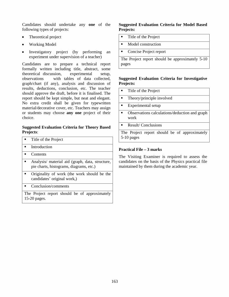
163

Candidates should undertake any one of the following types of projects:

• Theoretical project

• Working Model

• Investigatory project (by performing an experiment under supervision of a teacher)

Candidates are to prepare a technical report formally written including title, abstract, some theoretical discussion, experimental setup, observations with tables of data collected, graph/chart (if any), analysis and discussion of results, deductions, conclusion, etc. The teacher should approve the draft, before it is finalised. The report should be kept simple, but neat and elegant. No extra credit shall be given for typewritten material/decorative cover, etc. Teachers may assign or students may choose any one project of their choice.

Suggested Evaluation Criteria for Theory Based Projects:

Title of the Project

Introduction

Contents

Analysis/ material aid (graph, data, structure, pie charts, histograms, diagrams, etc.)

Originality of work (the work should be the candidates’ original work,)

Conclusion/comments

The Project report should be of approximately 15-20 pages.

Suggested Evaluation Criteria for Model Based Projects:

Title of the Project

Model construction

Concise Project report

The Project report should be approximately 5-10 pages

Suggested Evaluation Criteria for Investigative Projects:

Title of the Project

Theory/principle involved

Experimental setup

Observations calculations/deduction and graph work

Result/ Conclusions

The Project report should be of approximately 5-10 pages

Practical File – 3 marks

The Visiting Examiner is required to assess the candidates on the basis of the Physics practical file maintained by them during the academic year.