Correspondence analysis as an exploratory technique for stratigraphie abundance data

Trevor Ringrose Department of Probability and Statistics, University of Sheffield

1.1 Introduction

This paper describes the use of Correspondence Analysis (also known as dual scaling or Reciprocal Averaging) in initial investigations of abundance data from a sequence of strata. The technique, closely related mathematically to Principal Components Analysis, produces a graphical display of the rows and columns of a data matrix illustrating clusters within the rows and within the columns and the associations between them. Principal Components Analyses performed separately on the rows and columns would provide some of this information; Corre- spondence Analysis provides the link between them. The analysis is particularly appropriate to stratigraphie abundance data (of pollen, MNI indices or even artifacts) providing information on ecological groupings of layers and the associated indicator groupings of species. Initial visual inspection can be supplemented by computer-based simulation or 'bootstrapping' to assess statistical stability of observed groupings and overlaps. The techniques are illustrated on A. L. Armstrong's data from Pinhole Cave, Creswell Crags. These data give the MNI's for 148 vertebrate species in 21 stratigraphie layers. Henceforth multivariate data is taken to mean data where there are a group of objects each of which has a numerical value for each of a group of variables, and all of the objects arise 'on the same footing', that is none are viewed as responses to others. Stratigraphie abundance data are a special case of this where, depending on which is of most interest, the 'objects' are stratigraphie layers and the 'variables' species (or tool types etc) or vice-versa, and the values are the abundances.

1.2 Principal Components Analysis

Principal Components Analysis is a widely-used method for the preliminary investigation of multivariate data. It treats the values of the variables as the coordinates of the objects and, geometrically speaking, rotates the objects onto a new coordinate system. For example, with stratigraphie abundance data where interest is in the species (i.e. species are 'objects' and layers are 'variables') then the abundances of a species in the different layers are that species' coordinates; that is the layers are the 'dimensions' of the coordinate system. Thus each object has a new set of coordinates calculated from the old set such that each successive coordinate (i.e. dimension) accounts for the largest possible amount of the (remaining) variance (variation) in the data. The idea is that variance quantifies 'information' so that the first few coordinate axes, or 'principal components', contain the main feamres of the data, without a major loss

TREVOR RINGROSE

CM

X

.31

.20

•\|,3 •8

•7 .88

•e •5

•9 ' -.21 '«L.03 :8',2 .13 .'Z'l .35 -Vé .57

• 1 .69 .80

XI02 .91

•E -.!•»

•3

.12,,— •STRATIGRAPHIC LAYER • 11

•ie -.36

-.•^8

-.58

-.78

AXIS 1

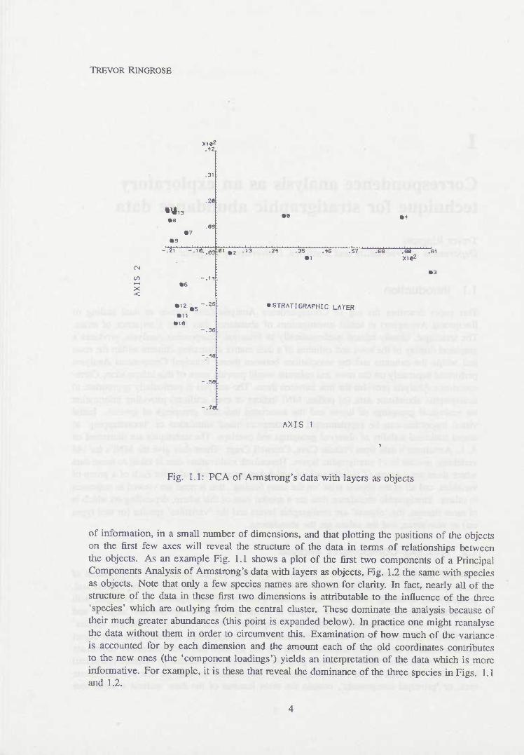
Fig. 1.1: PCA of Armstrong's data with layers as objects

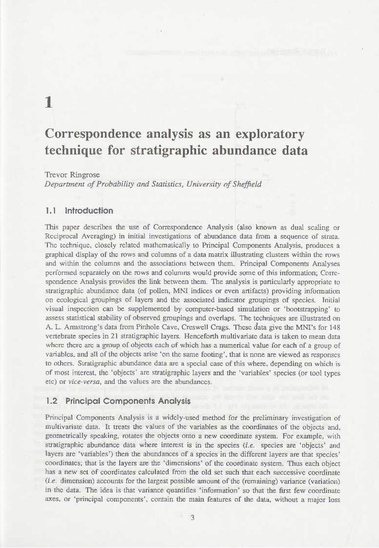
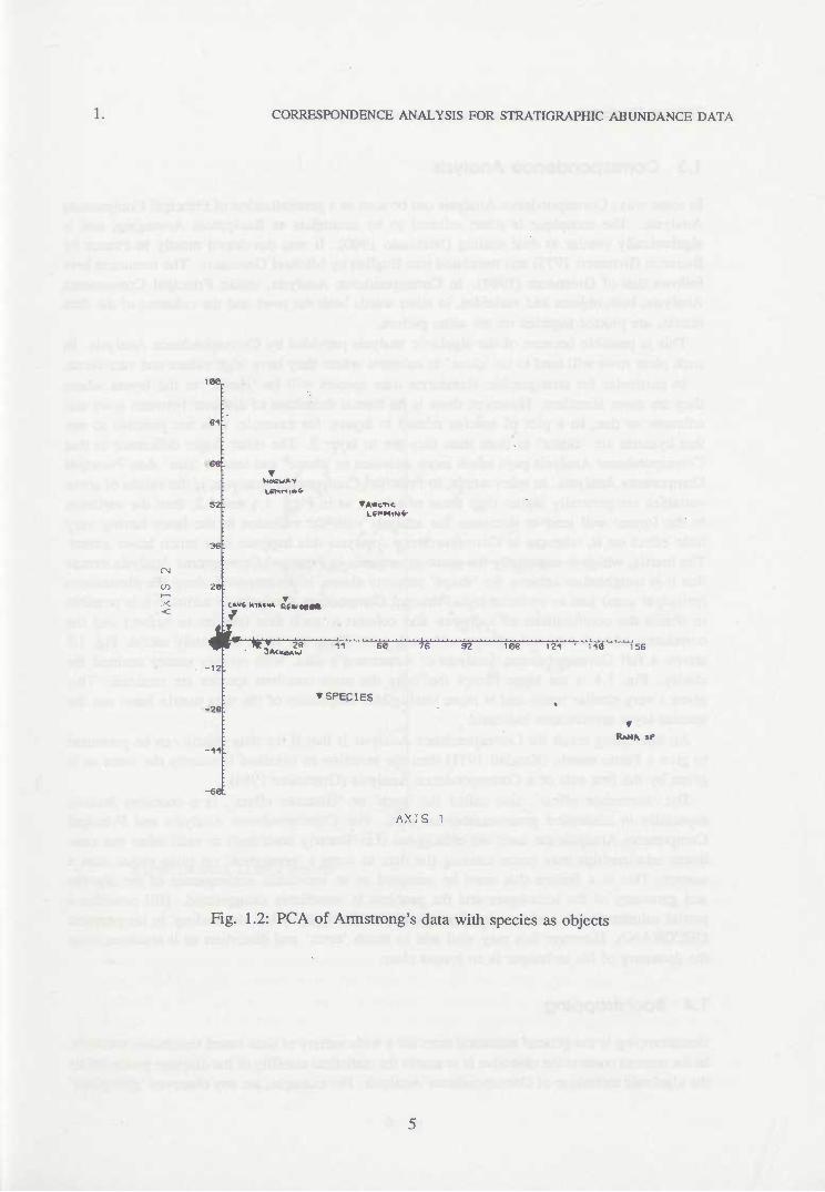
of information, in a small number of dimensions, and that plotting the positions of the objects on the first few axes wiU reveal the structure of the data in terms of relationships between the objects. As an example Fig. 1.1 shows a plot of the first two components of a Principal Components Analysis of Armstrong's data with layers as objects. Fig. 1.2 the same with species as objects. Note that only a few species names are shown for clarity. In fact, nearly all of the structure of the data in these first two dimensions is attributable to the influence of the three 'species' which are outlying from the central cluster. These dominate the analysis because of their much greater abundances (this point is expanded below). In practice one might reanalyse the data without them in order to circumvent this. Examination of how much of the variance is accounted for by each dimension and the amount each of the old coordinates contributes to the new ones (the 'component loadings') yields an interpretation of the data which is more informative. For example, it is these that reveal the dominance of the three species in Figs. 1.1 and 1.2.

CORRESPONDENCE ANALYSIS FOR STRATIGRAPHIC ABUNDANCE DATA

<

laa.

S2:

36:

28:

•*«ct<c

Cf^uc MYMMA atrnttm

-12.

^«8:

-6flt

ifr 28 11 60 76 92 lae 121 • 110 156

•SPECIES

RMIM if

AXIS 1

Fig. 1.2: PCA of Armstrong's data with species as objects

TREVOR RINGROSE

1.3 Correspondence Analysis

In some ways Correspondence Analysis can be seen as a generalisation of Principal Components Analysis. The technique is often referred to by ecologists as Reciprocal Averaging, and is algebraically similar to dual scaling (Nishisato 1980). It was developed mostly in France by Benzeen (Benzecri 1973) and translated into English by Michael Greenacre. The treatment here foUows that of Greenacre (1984). In Correspondence Analysis, unlike Principal Components Analysis, both objects and variables, in other words both the rows and the columns of the data matrix, are plotted together on the same picture.

This is possible because of the algebraic analysis provided by Correspondence Analysis. In such plots rows will tend to be 'close' to columns where they have high values and vice-versa.

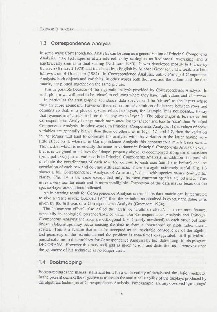
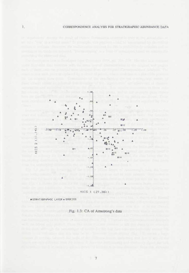
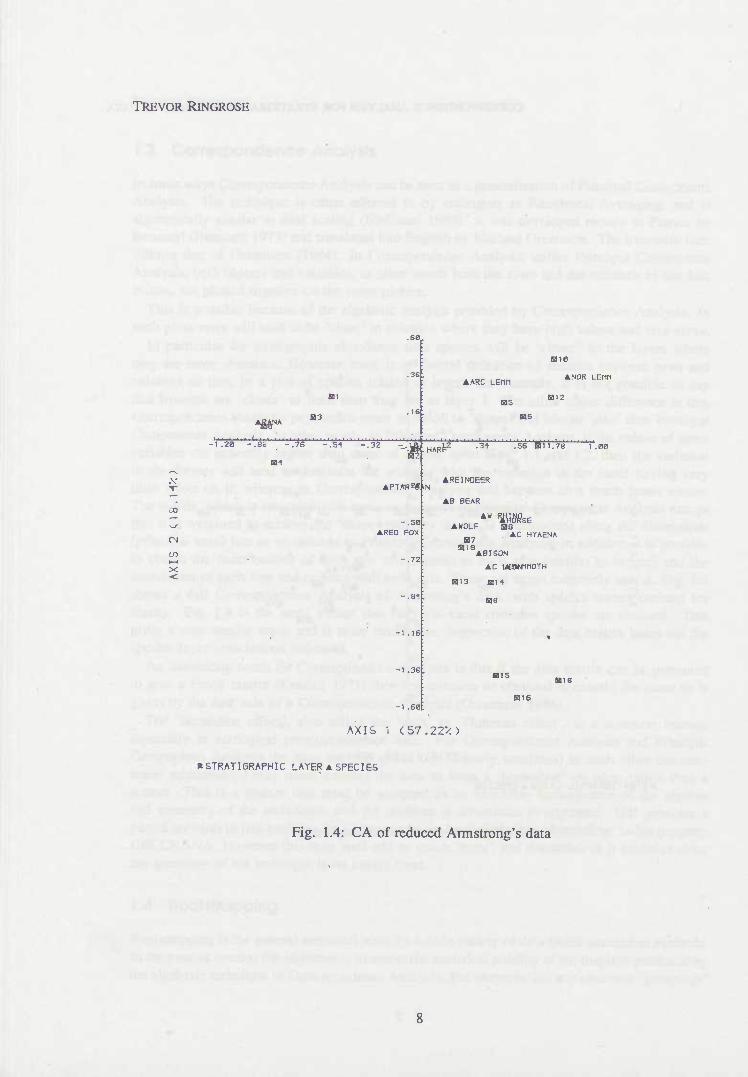
In particular for stratigraphie abundance data species will be 'closer' to the layers where they are more abundant. However, there is no formal definition of distance between rows and columns so that, in a plot of species related to layers, for example, it is not possible to say that hyaenas are 'closer' to lions than they are to layer 3. The other major difference is that Correspondence Analysis pays much more attention to 'shape* and less to 'size' than Principal Components Analysis. In other words, in Principal Components Analysis, if the values of some variables are generally higher than those of others, as in Figs. 1.1 and 1.2, then the variation in the former will tend to dominate the analysis with the variation in the latter having very little effect on it, whereas in Correspondence Analysis this happens to a much lesser extent. The inertia, which is essentially the same as variance in Principal Components Analysis except that it is weighted to achieve the 'shape' property above, is decomposed along the dimensions (principal axes) just as variance is in Principal Components Analysis; in addition it is possible to obtain the contributions of each row and column to each axis (similar to before) and the correlation of each row and column with each axis. These are again extremely useful. Fig. 1.3 shows a full Correspondence Analysis of Armstrong's data, with species names omitted for clarity. Fig. 1.4 is the same except that only the most common species are retained. This gives a very similar result and is more intelligible. Inspection of the data matrix bears out the species-layer associations indicated.

An interesting result for Correspondence Analysis is that if the data matrix can be permuted to give a Pétrie matrix (Kendall 1971) then the seriation so obtained is exactly the same as is given by the first axis of a Correspondence Analysis (Greenacre 1984).

The 'horseshoe effect', also called the 'arch' or 'Guttman effect', is a common feature, especially in ecological presence/absence data. For Correspondence Analysis and Principal Components Analysis the axes are orthogonal {i.e. lineariy unrelated) to each other but non- linear relationships may occur causing the data to form a 'horseshoe' on plots rather than a scatter. This is a feature that must be accepted as an inevitable consequence of the algebra and geometry of the techniques and the problem is sometimes exaggerated. Hill provides a partial solution to this problem for Correspondence Analysis by his 'detrending' in his program DECORANA. However this may well add as much 'error' and distortion as it removes since the geometry of his technique is no longer clear.

1.4 Bootstrapping

Bootstrapping is the general statistical term for a wide variety of data-based simulation metiiods. In tiie present context the objective is to assess the statistical stability of tiie displays produced by the algebraic technique of Correspondence Analysis. For example, are any observed 'groupings'

1. CORRESPONDENCE ANALYSIS FOR STRATIGRAPHIC ABUNDANCE DATA

à

30

.58

"f

A . A A à*

^ I ' M • ' • ' • 1 • ' I ' • ' ' ' • I • lii ' ' I ' ' • I I I I J....l.>.l..i.X I 1 li 1 i.J-U ,I.X.,i.l. -1 .50 -1 .19 -Î884 -19374 -.»•ö*»*05

* / A A

to

.38:

A. EG

A

fas

. I • 1.1 • 1. 111 • .36 .67 (au-98 1.29 1.60

A A

* Hl^ *

* ^ A i . ^ ait AA

813 B9

HIS aiS BS

B16

-1 .59

-1 .set

AXIS 1 (27.38k)

• STRATIGR.APHIC L.^YËR A SPECIES

Fig. 1.3: CA of Armstrong's data

TREVOR RINGROSE

.se

^êN* B3

-1.20 -.Sfc -.7e-.51 -.32

BB1

.V

CO

<

APTWÏ« kN

-.50 ARED FOX

-1 .38

-).601

AXIS I (57.22"^)

ggi0

AARC LEnn

B15

B6

HARÈ .3^ .SS B11.781.00

AREINDEER

AB BEAR

A WOLF as „, . AC HYAENA H7

BI'-S AB! SON

AC lAinMiriOTH

B13 SI11

BS

BIS

116

ISTRAT ISRAPHIC LATER A SPECIES

Fig. 1.4: CA of reduced Annstrong's data

1. CORRESPONDENCE ANALYSIS FOR STRATIGRAPHIC ABUNDANCE DATA

or 'separations' merely the result of chance fluctuations observable only in the actual data or are they 'real' in a wider sense? In principle, this problem could be investigated by theoretical statistical analysis. However, the mathematics required for this is prohibitively complex and so simulation methods are required. 'Bootstrapping' is a form of simulation based on statistically perturbing the observed data.

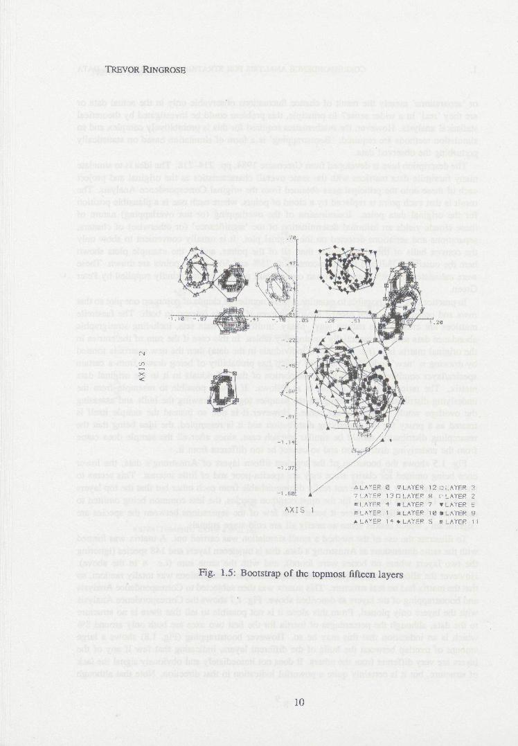
The description here is developed from Greenacre 1984, pp. 214-218. The idea is to simulate many facsimile data matrices with the same overall characteristics as the original and project each of these onto the principal axes obtained from the original Correspondence Analysis. The result is that each point is replaced by a cloud of points, where each one is a plausible position for the original data point. Examination of the overlapping (or not overlapping) nature of these clouds yields an informal determination of the 'significance' (or otherwise) of clusters, separations and seriations detected on the original plot. It is usually convenient to show only the convex huUs of the clouds rather than all of the points, and in the example plots shown here the outermost hull and the hulls containing 75% and 50% of the points are drawn. These were calculated by the Green-Silverman convex hull peeling routine, kindly supplied by Peter Green.

In practice it is only possible to examine a small number of clouds of points on one plot so that rows and columns are often plotted separately even if there is interest in both. The facsimile matrices are created in a natural way. Many 'multivariate' data sets, including stratigraphie abundance data sets, are essentially contingency tables. In this case if the sum of the entries in the original matrix is n (i.e. there are n individuals in the data) then the new matrix is formed by drawing n 'new' individuals, each of which has probability of being drawn from a certain speciesAayer combination equal to the proportion of the individuals in it in the original data matrix. The rationale behind all this is as follows. If it was possible to resample from the underlying distribution then plotting all the samples together, drawing the huUs and assessing the overlaps would certainly make sense. However it is not, so instead the sample itself is treated as a proxy for the underlying distribution and it is resampled, the idea being that the resampling distribution should be similar in each case, since after, aU the sample does come from the tmderlying distribution and so carmot be too different from it.

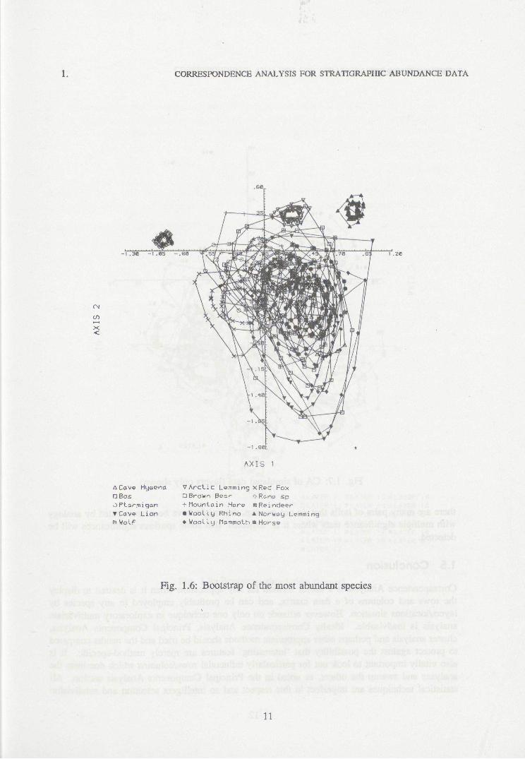
Fig. 1.5 shows the bootstrap of the topmost fifteen layers of Armstrong's data, the lower ones being omitted for clarity since they are species-poor and of little interest. This seems to show that the lower layers are not reaUy distinguishable from each other but that the top layers are. Fig. 1.6 shows the same for the most common species, the less common being omitted to make the plot intelligible. Here it seems that few of the separations between the species are 'significant', which makes sense as nearly all are cold-stage animals.

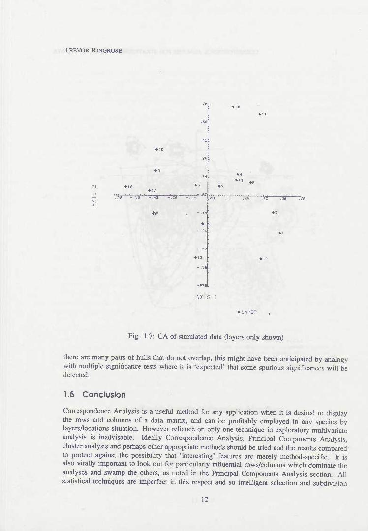
To illustrate the use of the method a small simulation was carried out. A matrix was formed with the same dimensions as Armstrong's data, that is nineteeen layers and 148 species (ignoring the two layers where no bones were found), and with the same sum (i.e. n in the above). However the allocation of the individuals to species/layer combinations was totally random, so that the matrix had no real structure. This matrix was then subjected to Correspondence Analysis and bootstrapping of the layers aS described above. Fig. 1.7 shows the Correspondence Analysis with the layers only plotted. From this alone it is not possible to tell that there is no structure to the data, although the percentages of inertia for the first two axes are both only around 8% which is an indication that this may be so. However bootstrapping (Fig. 1.8) shows a large amount of overlap between the huUs of the different layers, indicating that few if any of the layers are very different from the others. It does not immediately and obviously signal the lack of structure, but it is certainly quite a powerful indication in that direction. Note that although

TREVOR RINGROSE

A LAYER 0 7 LAYER 12 nLAYER 3 7 LAYER l?n LAYER 8 (LAYER 2 »LAYER ^ «LAYER 7 T LAYER S a LAYER 1 SLAYER 1 0 • LAYER 9 * LAYER I'f» LAYER 5 »LAYER 11

Fig. 1.5: Bootstrap of the topmost fifteen layers

10

1. CORRESPONDENCE ANALYSIS FOR STRATIGRAPHIC ABUNDANCE DATA

if)

X <

ACave Hyoena VArctic Lemming xRed Fox DBos nBrown Bear oRono sp oPtormigan fdountain Hare B Reindeer ^ Cave Lion «WooLl-g Rhino A Norway Lemming B WolF •Woolly Mammoth » Horse

Fig. 1.6: Bootstrap of the most abundant species

11

TREVOR RINGROSE

X <

.7a • 16

• n .56

.12

• ie

.28 [

• 19

•3

• 17 • 1

.M

• 6

, ,

• 1

•'^ •S • 7

.72 -.56 -.12 -.28 -.11

-.11

• 1 -.28

-.12

• 13

-.56

-*7t

,00

:

•

:

.11 .28 .12 .56

•2

• i

• 12

.70

AXIS 1

•LAYER

Fig. 1.7: CA of simulated data Oayers only shown)

there are many pairs of hulls that do not overlap, this might have been anticipated by analogy with multiple significance tests where it is 'expected' that some spurious significances will be detected.

1.5 Conclusion

Correspondence Analysis is a useful method for any application when it is desired to display the rows and columns of a data matrix, and can be profitably employed in any species by layers/locations situation. However reliance on only one technique in exploratory multivariate analysis is inadvisable. Ideally Correspondence Analysis, Principal Components Analysis, cluster analysis and perfiaps other appropriate methods should be tried and the results compared to protect against the possibility that 'interesting' features are merely method-specific. It is also vitally important to look out for particularly influential rows/columns which dominate the analyses and swamp the others, as noted in the Principal Components Analysis section. All statistical techniques are imperfect in this respect and so intelligent selection and subdivision

12

1. CORRESPONDENCE ANALYSIS FOR STRATIGRAPHIC ABUNDANCE DATA

U5

X <

AXIS 1 ALAYER nLAYER DLAYER • LAYER »LAYER A LAYER • LAYER

1 V LAYER 't V LAYER 9 O LAYER 8 T LAYER 1 1 «LAYER 15 BLAYER 12

13 PLAYER M X LAYER 3 »LAYER 7 ts LAYER 17 »LAYER 18 • LAYER

19 16 5 2

Fig. 1.8: Bootstrap simulation (layers)

13

TREVOR RINGROSE

of the data is worthwhile. Examination of the contributions of rows and columns to the axes in Correspondence Analysis and Principal Components Analysis should reveal these. It is not adequate to plot the data on the first two axes and base conclusions solely on that picture, as is all too frequently the practice.

References

BENZECRI, J. 1973. LAnalysée des Données. Tome 1: La Taxinomie. Tome 2: L'Analyse des Correspondances, Dunod, Paris.

GREENACRE, M. J. 1984. Theory and Applications of Correspondence Analysis, Academic Press, London.

KENDALL, D. G. 1971. 'Seriation from abundance matrices', in C. R. Hodson, D. G. Kendall, & P. Tautu, (eds.), Mathematics in the Archaeologiccd and Historical Sciences, pp. 215-252, Edinburgh University Press, Edinburgh.

NismsATO, S. 1980. Analysis of Categorical Data: Dual Scaling and its Applications, Univer- sity of Toronto Press, Toronto.

14