Copyright © Cengage Learning. All rights reserved.

Power FunctionsSECTION 5.2

2

Learning Objectives

1 Use power functions to model real-world situations

2 Use the language of rate of change to describe the behavior of power functions

3 Determine whether a power function represents direct or inverse variation

3

Power Functions

4

Power Functions

Migrating land animals, such as caribou, are called runners.

Runners migrate seasonally from one region to another.

The migration speed of such animals, in kilometers per day, is dependent on the mass of the animal, given in kilograms.

5

Power Functions

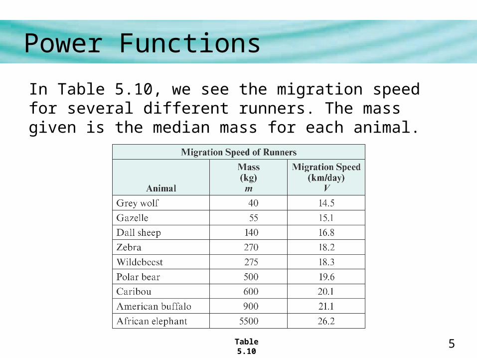
In Table 5.10, we see the migration speed for several different runners. The mass given is the median mass for each animal.

Table 5.10

6

Power Functions

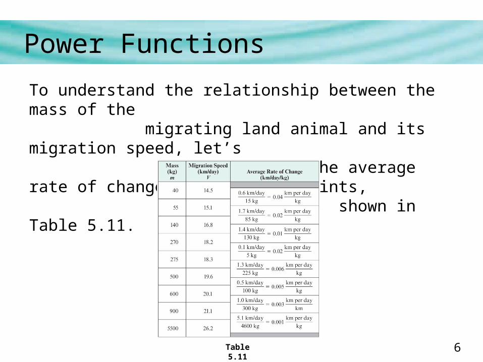
To understand the relationship between the mass of the migrating land animal and its migration speed, let’s consider the average rate of change between data points, shown in Table 5.11.

Table 5.11

7

Power Functions

Observe that the rate of change is approaching zero.

That is, as the mass of the animal increases, the number of additional kilometers per day that it travels when 1 additional kilogram is added to its mass approaches 0 kilometers.

8

Power Functions

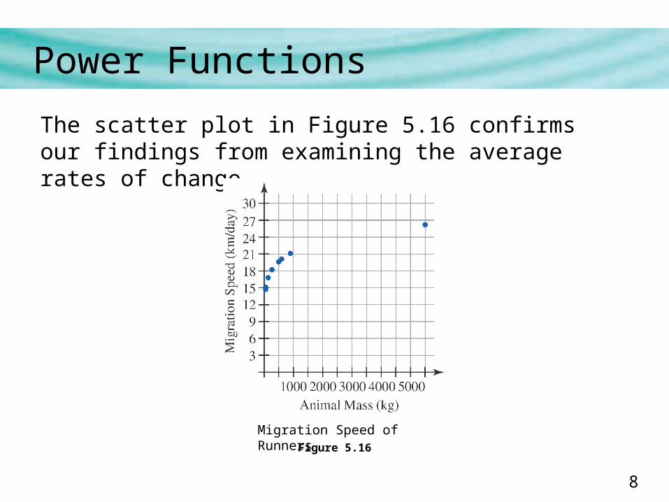
The scatter plot in Figure 5.16 confirms our findings from examining the average rates of change.

Figure 5.16

Migration Speed of Runners

9

Power Functions

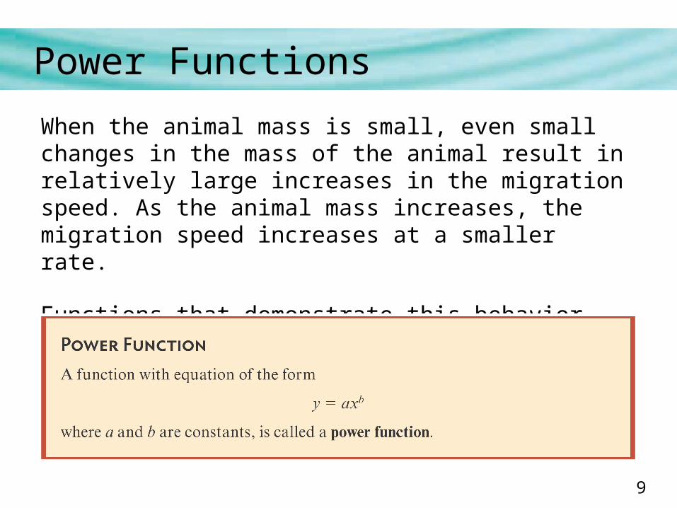
When the animal mass is small, even small changes in the mass of the animal result in relatively large increases in the migration speed. As the animal mass increases, the migration speed increases at a smaller rate.

Functions that demonstrate this behavior can often be modeled with a power function.

10

Power Functions

One main difference between a power function and a polynomial function is that in a power function the exponent, b, can take on any real-number value rather than just positive integer values.

Also, a power function is a single-term function whereas a polynomial function may have multiple terms.

11

Example 1 – Using a Power Function in a Real-World Context

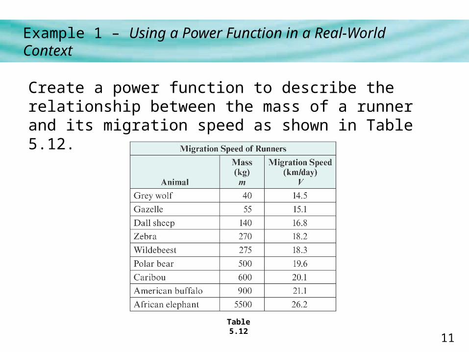
Create a power function to describe the relationship between the mass of a runner and its migration speed as shown in Table 5.12.

Table 5.12

12

Example 1 – Using a Power Function in a Real-World Context

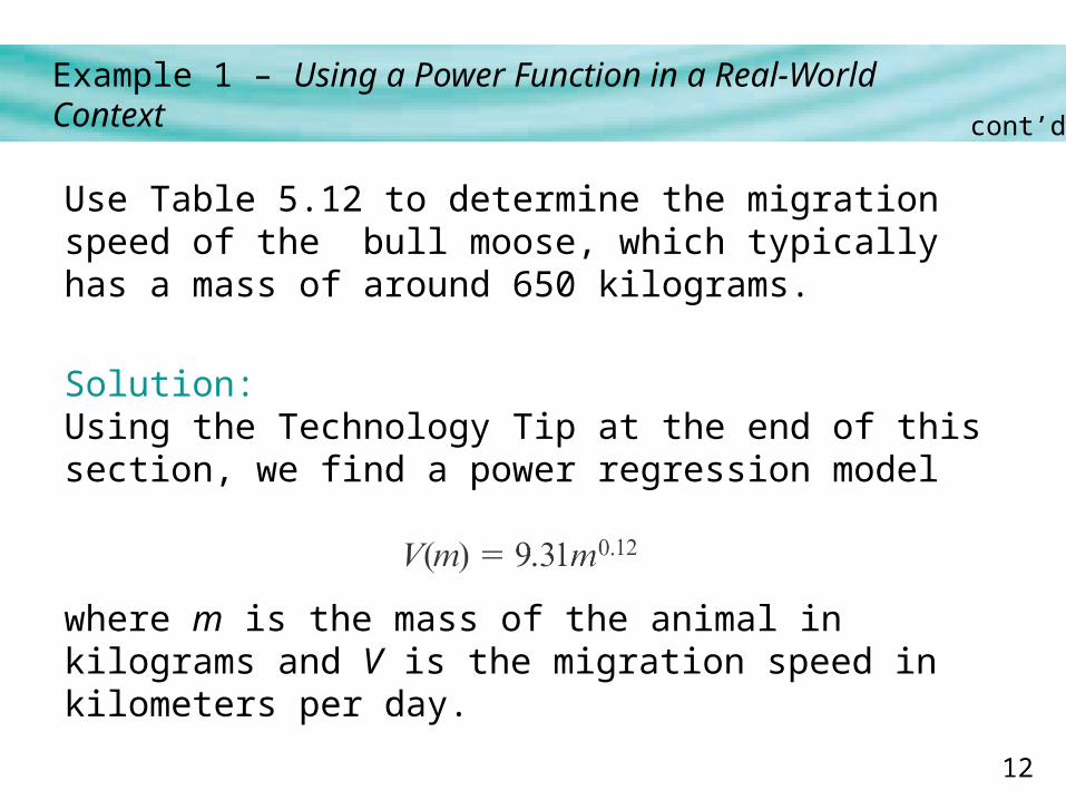
Use Table 5.12 to determine the migration speed of the bull moose, which typically has a mass of around 650 kilograms.

Solution:Using the Technology Tip at the end of this section, we find a power regression model

where m is the mass of the animal in kilograms and V is the migration speed in kilometers per day.

cont’d

13

Example 1 – Solution

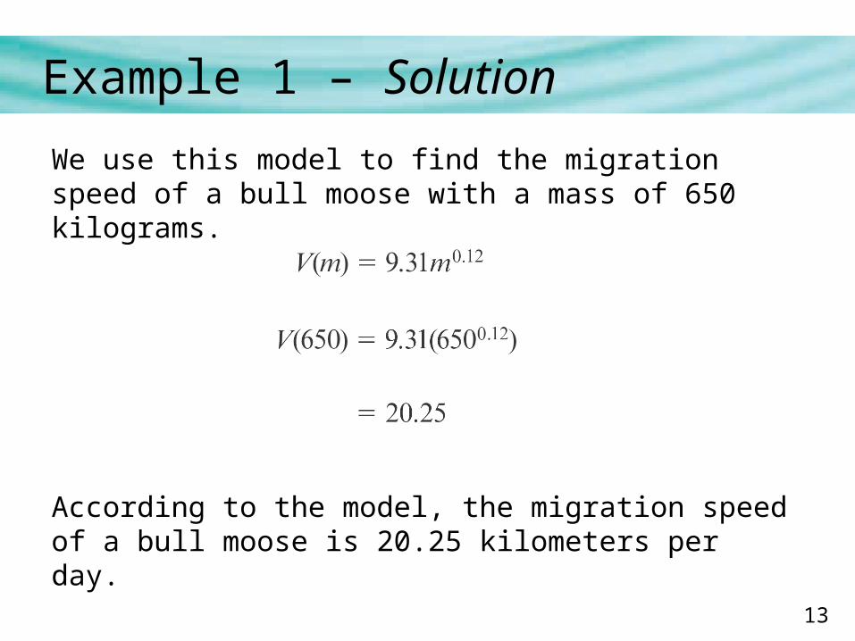
We use this model to find the migration speed of a bull moose with a mass of 650 kilograms.

According to the model, the migration speed of a bull moose is 20.25 kilometers per day.

14

Power Functions with x 0 and 0 < b < 1

15

Power Functions with x 0 and 0 < b < 1

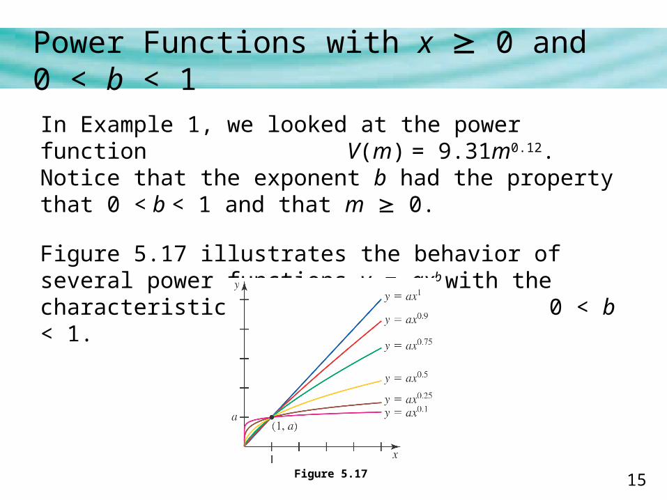
In Example 1, we looked at the power function V(m) = 9.31m0.12. Notice that the exponent b had the property that 0 < b < 1 and that m 0.

Figure 5.17 illustrates the behavior of several power functions y = axb with the characteristic that x 0 and 0 < b < 1.

Figure 5.17

16

Power Functions with x 0 and 0 < b < 1

We see that each power function contains the point (1, a) since 1b = 1 for all b.

Further, as b gets closer and closer to 1, the power function approaches the linear power function y = ax1.

17

Power Functions with x > 0 and b < 0

18

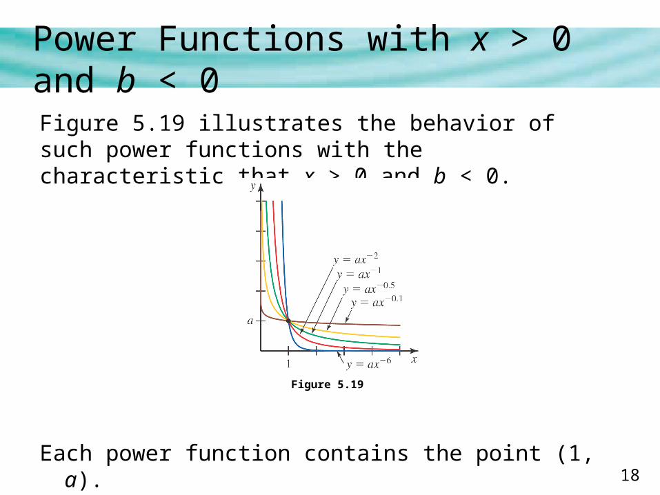
Power Functions with x > 0 and b < 0

Figure 5.19 illustrates the behavior of such power functions with the characteristic that x > 0 and b < 0.

Each power function contains the point (1, a).

Figure 5.19

19

Power Functions with x > 0 and b < 0

Also, the more negative the value of b, the more quickly the function values approach 0.

Furthermore, as b approaches 0, the power function gets closer and closer to the linear power function y = a.

20

Direct and Inverse Variation

21

Direct and Inverse Variation

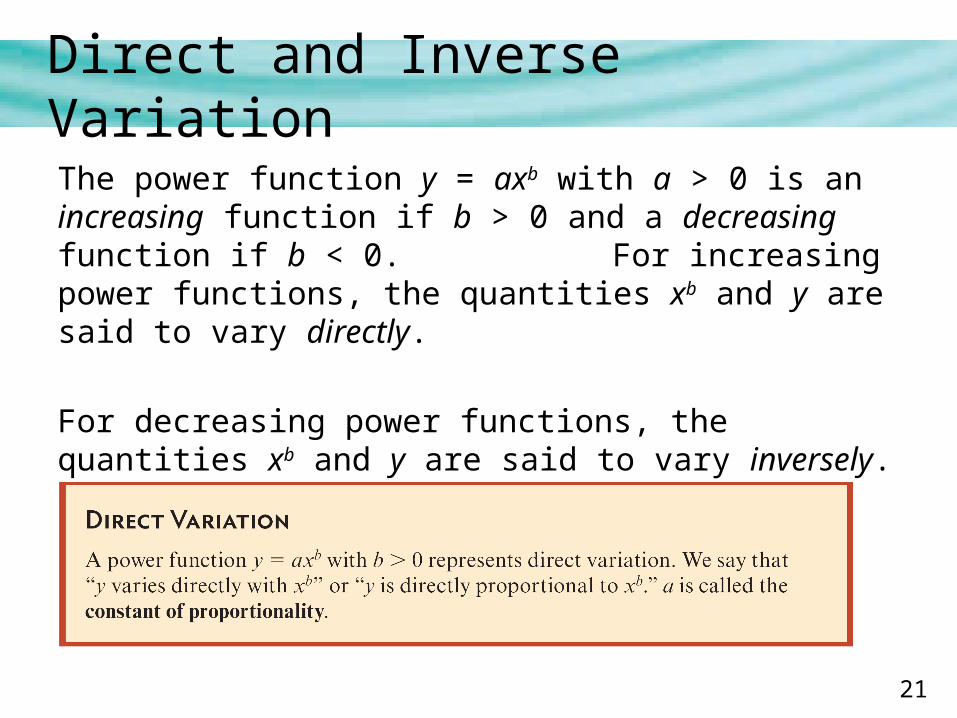
The power function y = axb with a > 0 is an increasing function if b > 0 and a decreasing function if b < 0. For increasing power functions, the quantities xb and y are said to vary directly.

For decreasing power functions, the quantities xb and y are said to vary inversely.

22

Direct and Inverse Variation

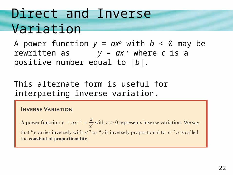
A power function y = axb with b < 0 may be rewritten as y = ax

–c where c is a positive number equal to |b|.

This alternate form is useful for interpreting inverse variation.

23

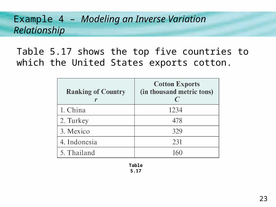
Example 4 – Modeling an Inverse Variation Relationship

Table 5.17 shows the top five countries to which the United States exports cotton.

Table 5.17

24

Example 4 – Modeling an Inverse Variation Relationship

a. By analyzing a scatter plot of the data and investigating rates of change, explain why a power function may best model the data.

b. Determine a power regression model to represent the data and use it to describe the relationship between the amount of cotton exports and the ranking of the country.

c. According to the model, how much cotton would the United States export to a country whose rank is 6?

cont’d

25

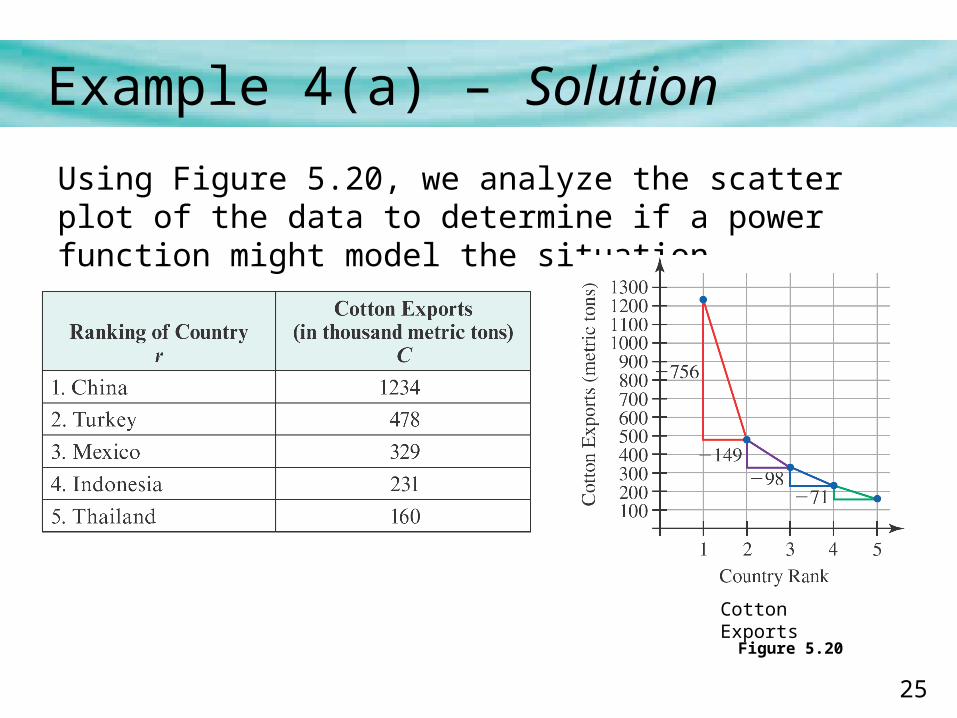
Example 4(a) – Solution

Using Figure 5.20, we analyze the scatter plot of the data to determine if a power function might model the situation.

Figure 5.20

Cotton Exports

26

Example 4(a) – Solution

We observe the rate of change is initially very dramatic but lessens as the country rank increases.

This is characteristic of a power function describing an inverse variation relationship between the quantities.

cont’d

27

Example 4(b) – Solution

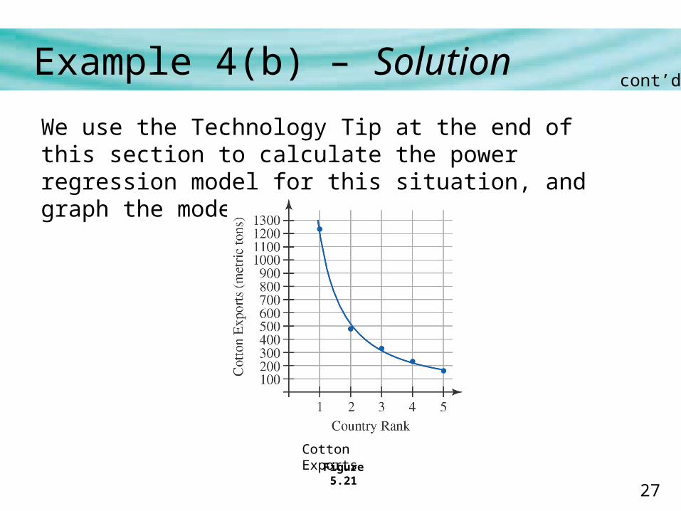
We use the Technology Tip at the end of this section to calculate the power regression model for this situation, and graph the model in Figure 5.21.

Figure 5.21

Cotton Exports

cont’d

28

Example 4(b) – Solution

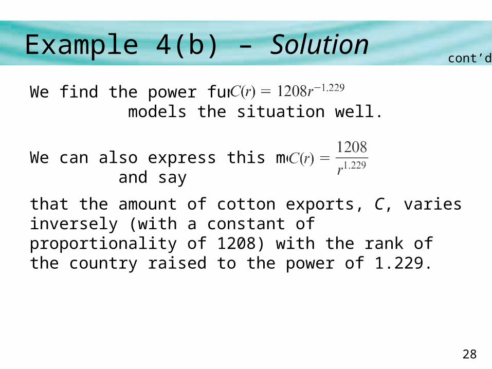
We find the power function models the situation well.

We can also express this model as and say

that the amount of cotton exports, C, varies inversely (with a constant of proportionality of 1208) with the rank of the country raised to the power of 1.229.

cont’d

29

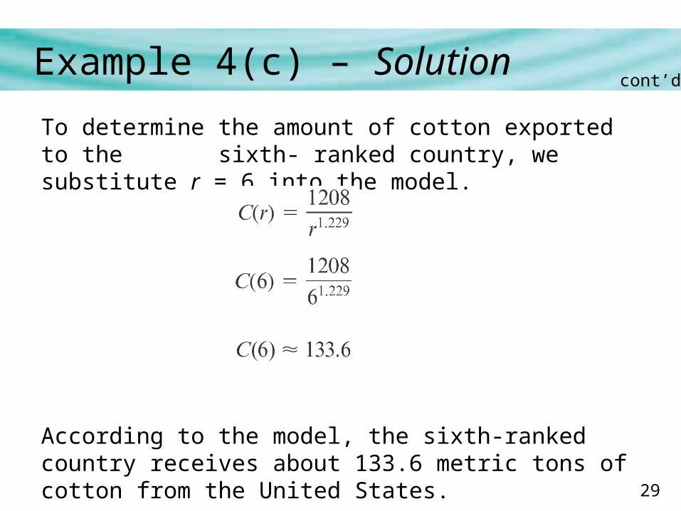
Example 4(c) – Solution

To determine the amount of cotton exported to the sixth- ranked country, we substitute r = 6 into the model.

According to the model, the sixth-ranked country receives about 133.6 metric tons of cotton from the United States.

cont’d

30

Inverses of Power Functions

31

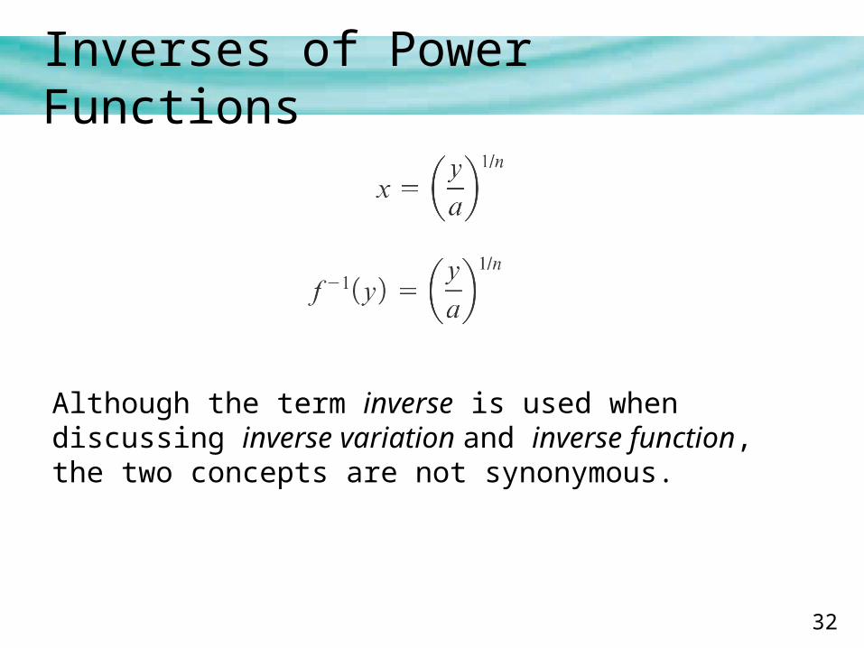
Inverses of Power Functions

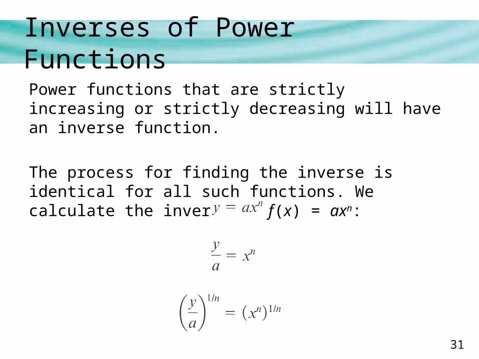
Power functions that are strictly increasing or strictly decreasing will have an inverse function.

The process for finding the inverse is identical for all such functions. We calculate the inverse of f (x) = axn:

32

Inverses of Power Functions

Although the term inverse is used when discussing inverse variation and inverse function, the two concepts are not synonymous.