Copyright © Cengage Learning. All rights reserved.

2.3 Real Zeros of Polynomial Functions

2

What You Should Learn

• Use long division to divide polynomials by other polynomials.

• Use synthetic division to divide polynomials by binomials of the form (x – k).

• Use the Remainder and Factor Theorems.

3

What You Should Learn

• Use the Rational Zero Test to determine possible rational zeros of polynomial functions.

• Use Descartes’s Rule of Signs and the Upperand Lower Bound Rules to find zeros of polynomials.

4

Long Division of Polynomials

5

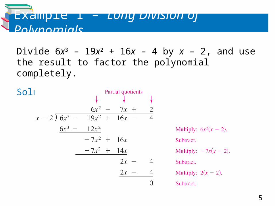
Example 1 – Long Division of Polynomials

Divide 6x3 – 19x2 + 16x – 4 by x – 2, and use the result to factor the polynomial completely.

Solution:

6

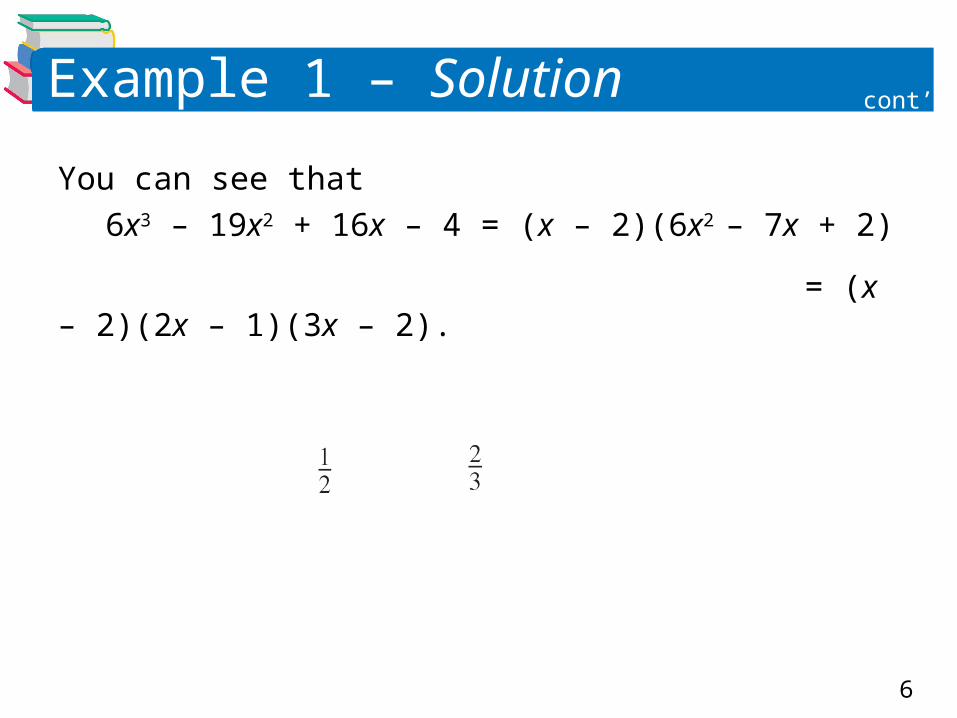
Example 1 – Solution

You can see that

6x3 – 19x2 + 16x – 4 = (x – 2)(6x2 – 7x + 2)

= (x – 2)(2x – 1)(3x – 2).

cont’d

7

Long Division of Polynomials

8

Synthetic Division

9

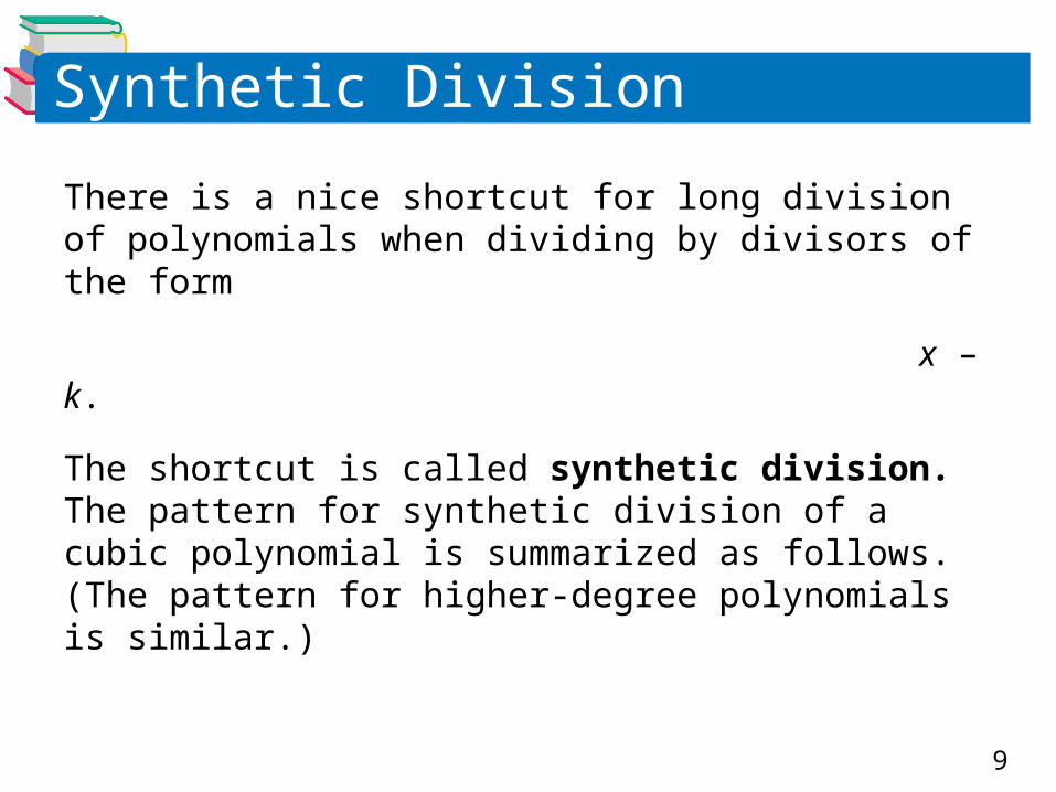
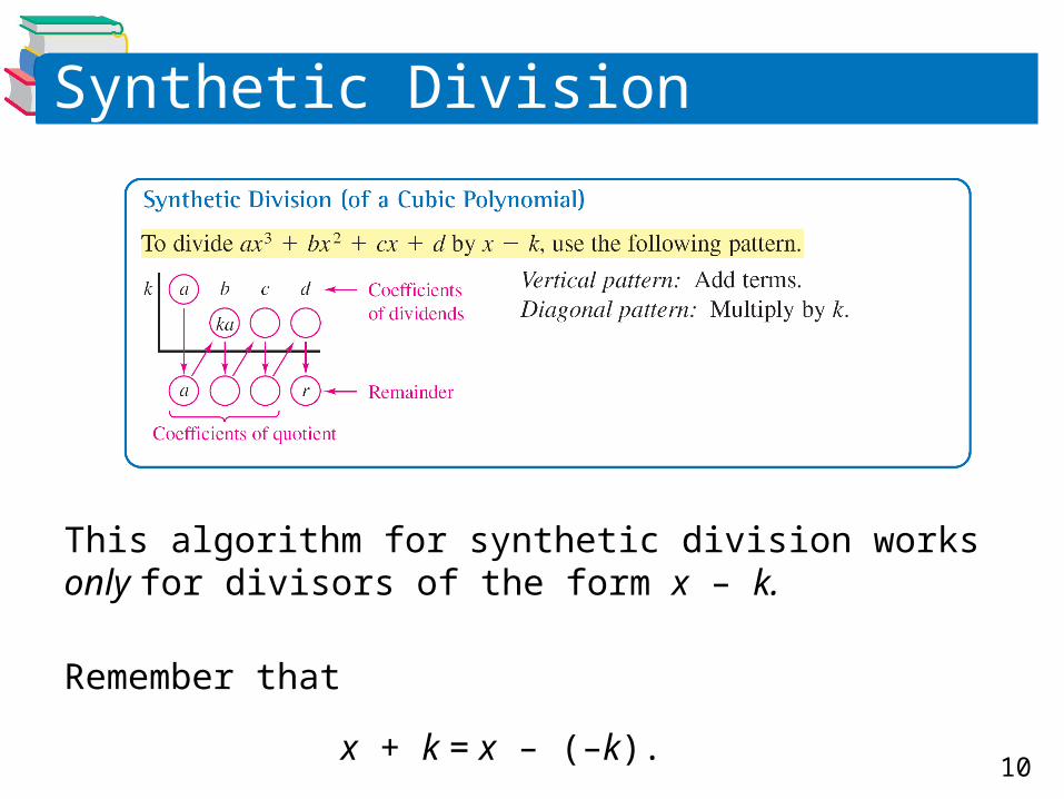
Synthetic Division

There is a nice shortcut for long division of polynomials when dividing by divisors of the form

x – k.

The shortcut is called synthetic division. The pattern for synthetic division of a cubic polynomial is summarized as follows. (The pattern for higher-degree polynomials is similar.)

10

Synthetic Division

This algorithm for synthetic division works only for divisors of the form x – k.

Remember that

x + k = x – (–k).

11

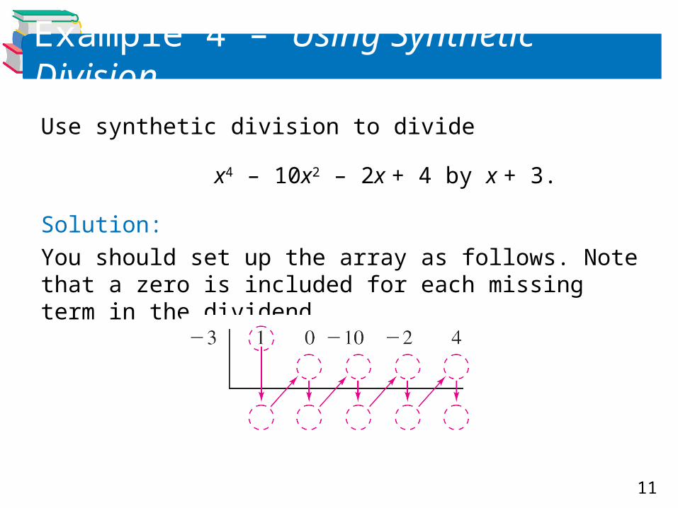
Example 4 – Using Synthetic Division

Use synthetic division to divide

x4 – 10x2 – 2x + 4 by x + 3.

Solution:

You should set up the array as follows. Note that a zero is included for each missing term in the dividend.

12

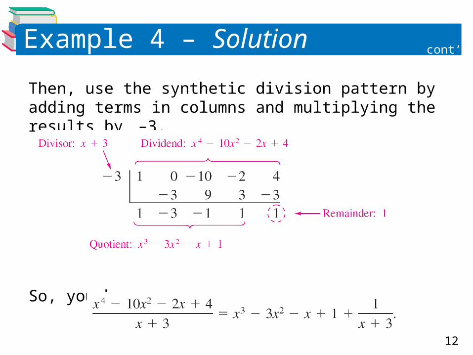
Example 4 – Solution

Then, use the synthetic division pattern by adding terms in columns and multiplying the results by –3.

So, you have

cont’d

13

The Remainder and Factor Theorems

14

The Remainder and Factor Theorems

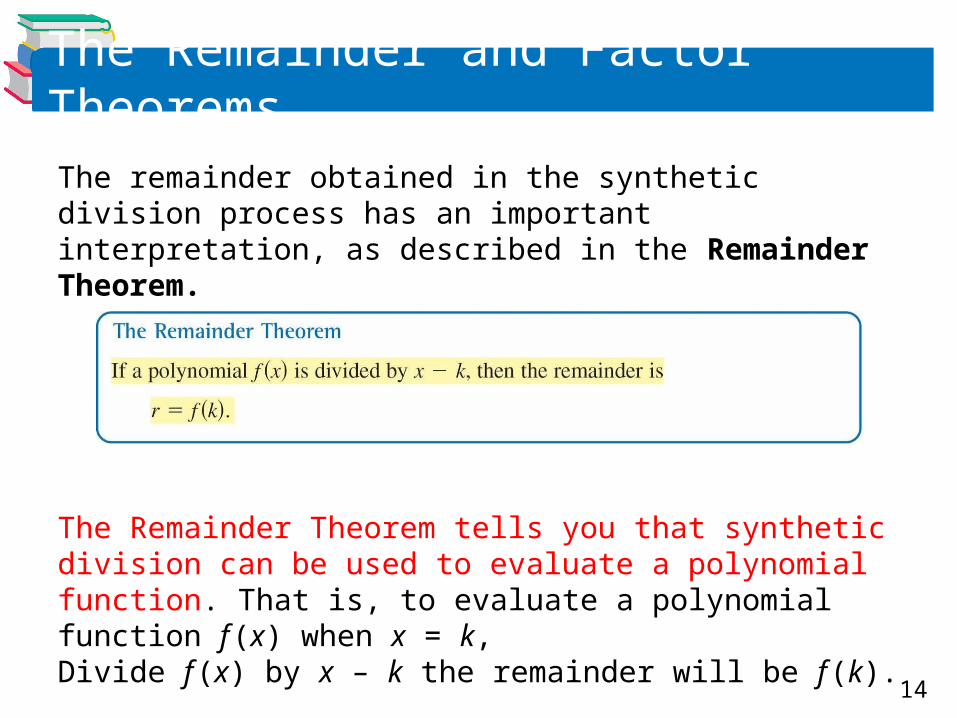
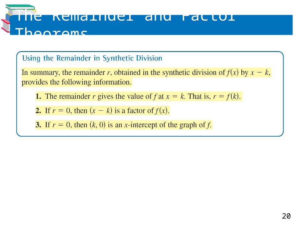
The remainder obtained in the synthetic division process has an important interpretation, as described in the Remainder Theorem.

The Remainder Theorem tells you that synthetic division can be used to evaluate a polynomial function. That is, to evaluate a polynomial function f (x) when x = k, Divide f (x) by x – k the remainder will be f (k).

15

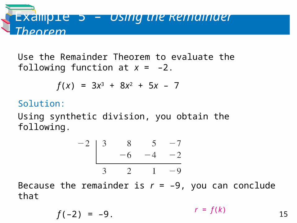
Example 5 – Using the Remainder Theorem

Use the Remainder Theorem to evaluate the following function at x = –2.

f (x) = 3x3 + 8x2 + 5x – 7

Solution:

Using synthetic division, you obtain the following.

Because the remainder is r = –9, you can conclude that

f (–2) = –9. r = f (k)

16

Example 5 – Solution

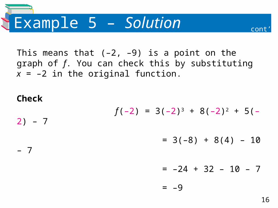
This means that (–2, –9) is a point on the graph of f. You can check this by substituting x = –2 in the original function.

Check

f (–2) = 3(–2)3 + 8(–2)2 + 5(–2) – 7

= 3(–8) + 8(4) – 10 – 7

= –24 + 32 – 10 – 7

= –9

cont’d

17

The Remainder and Factor Theorems

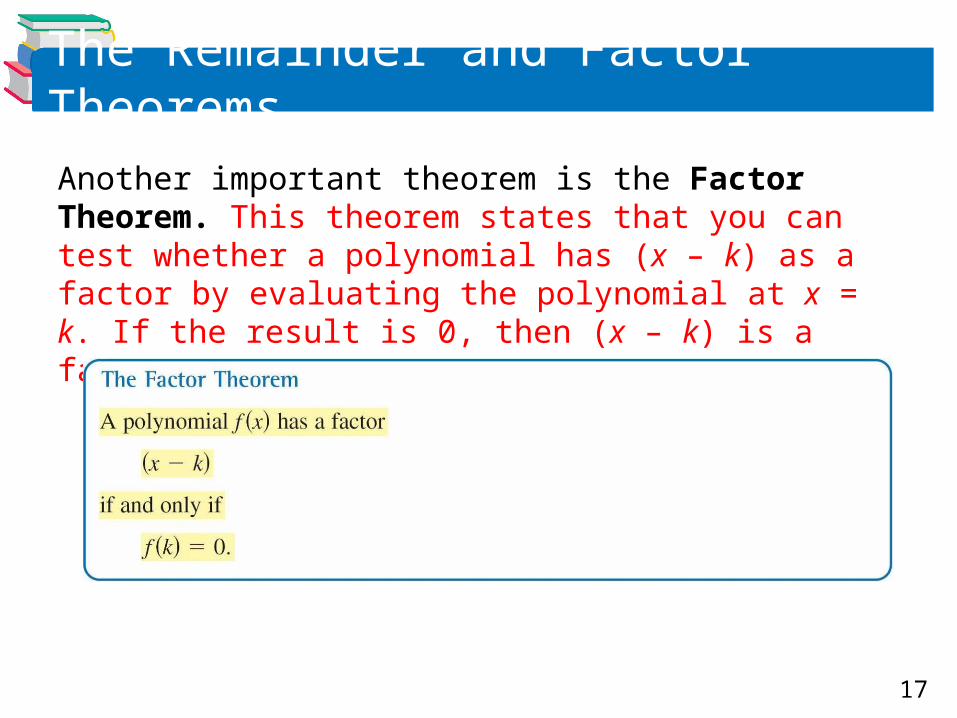
Another important theorem is the Factor Theorem. This theorem states that you can test whether a polynomial has (x – k) as a factor by evaluating the polynomial at x = k. If the result is 0, then (x – k) is a factor.

18

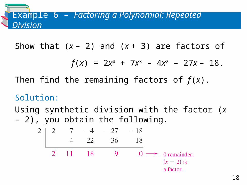
Example 6 – Factoring a Polynomial: Repeated Division

Show that (x – 2) and (x + 3) are factors of

f (x) = 2x4 + 7x3 – 4x2 – 27x – 18.

Then find the remaining factors of f (x).

Solution:

Using synthetic division with the factor (x – 2), you obtain the following.

19

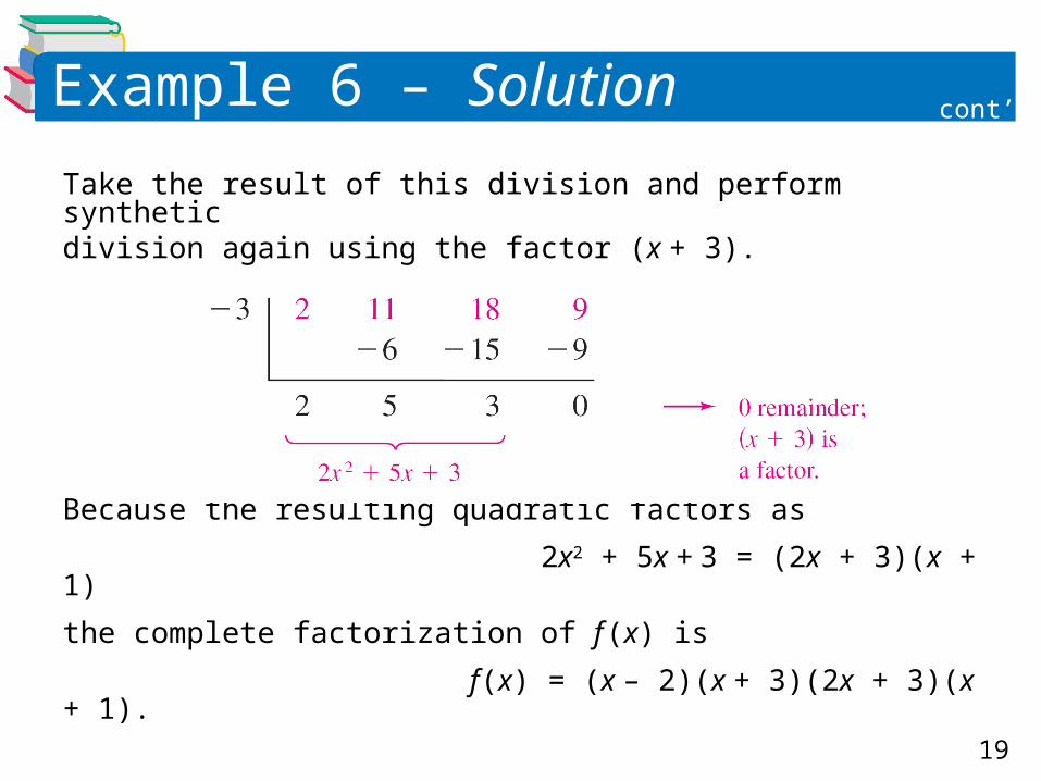
Example 6 – Solution

Take the result of this division and perform syntheticdivision again using the factor (x + 3).

Because the resulting quadratic factors as

2x2 + 5x + 3 = (2x + 3)(x + 1)

the complete factorization of f (x) is

f (x) = (x – 2)(x + 3)(2x + 3)(x + 1).

cont’d

20

The Remainder and Factor Theorems

21

The Rational Zero Test

22

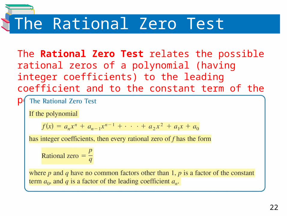
The Rational Zero Test

The Rational Zero Test relates the possible rational zeros of a polynomial (having integer coefficients) to the leading coefficient and to the constant term of the polynomial.

23

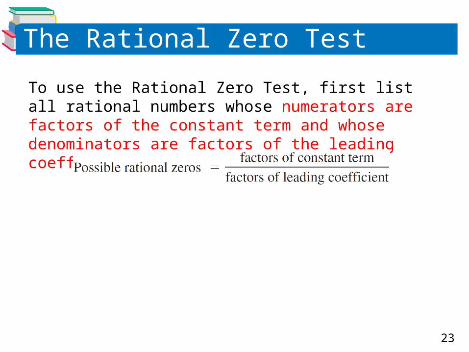
The Rational Zero Test

To use the Rational Zero Test, first list all rational numbers whose numerators are factors of the constant term and whose denominators are factors of the leading coefficient.

24

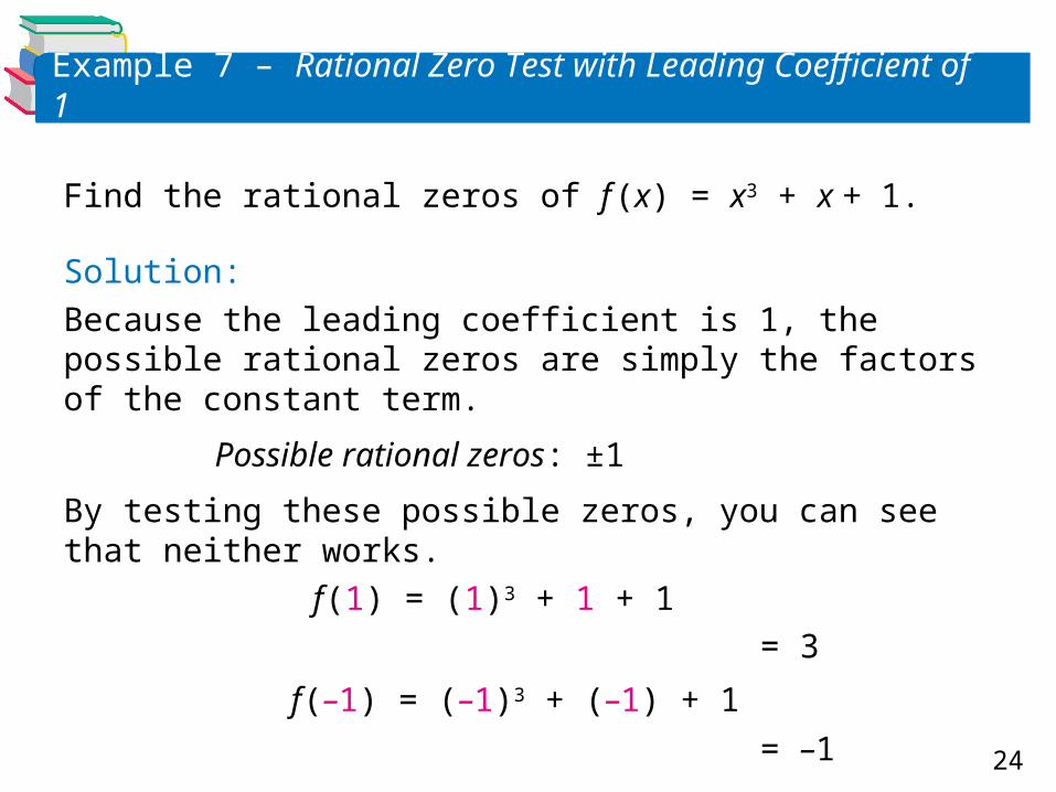
Example 7 – Rational Zero Test with Leading Coefficient of 1

Find the rational zeros of f (x) = x3 + x + 1.

Solution:

Because the leading coefficient is 1, the possible rational zeros are simply the factors of the constant term.

Possible rational zeros: ±1

By testing these possible zeros, you can see that neither works.

f (1) = (1)3 + 1 + 1

= 3

f (–1) = (–1)3 + (–1) + 1

= –1

25

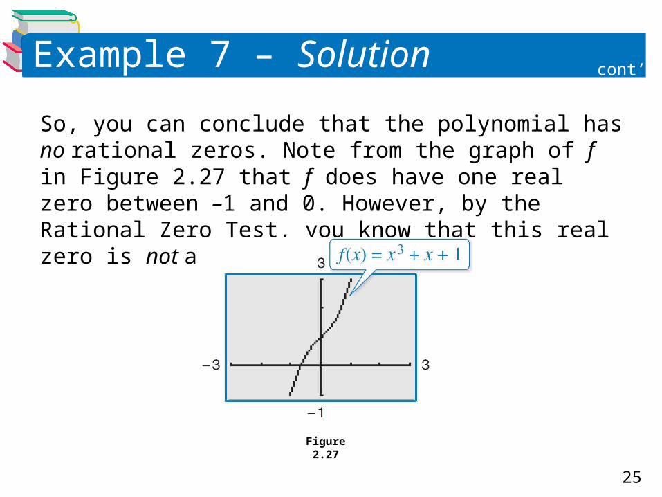
Example 7 – Solution

So, you can conclude that the polynomial has no rational zeros. Note from the graph of f in Figure 2.27 that f does have one real zero between –1 and 0. However, by the Rational Zero Test, you know that this real zero is not a rational number.

cont’d

Figure 2.27

26

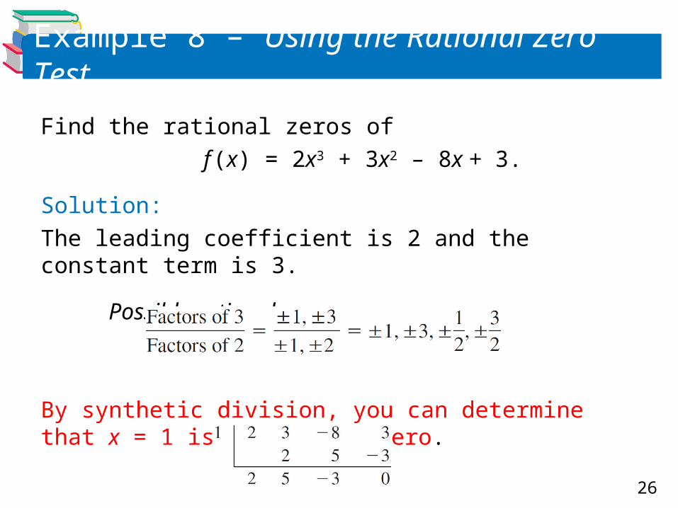
Example 8 – Using the Rational Zero Test

Find the rational zeros of

f (x) = 2x3 + 3x2 – 8x + 3.

Solution:

The leading coefficient is 2 and the constant term is 3.

Possible rational zeros:

By synthetic division, you can determine that x = 1 is a rational zero.

27

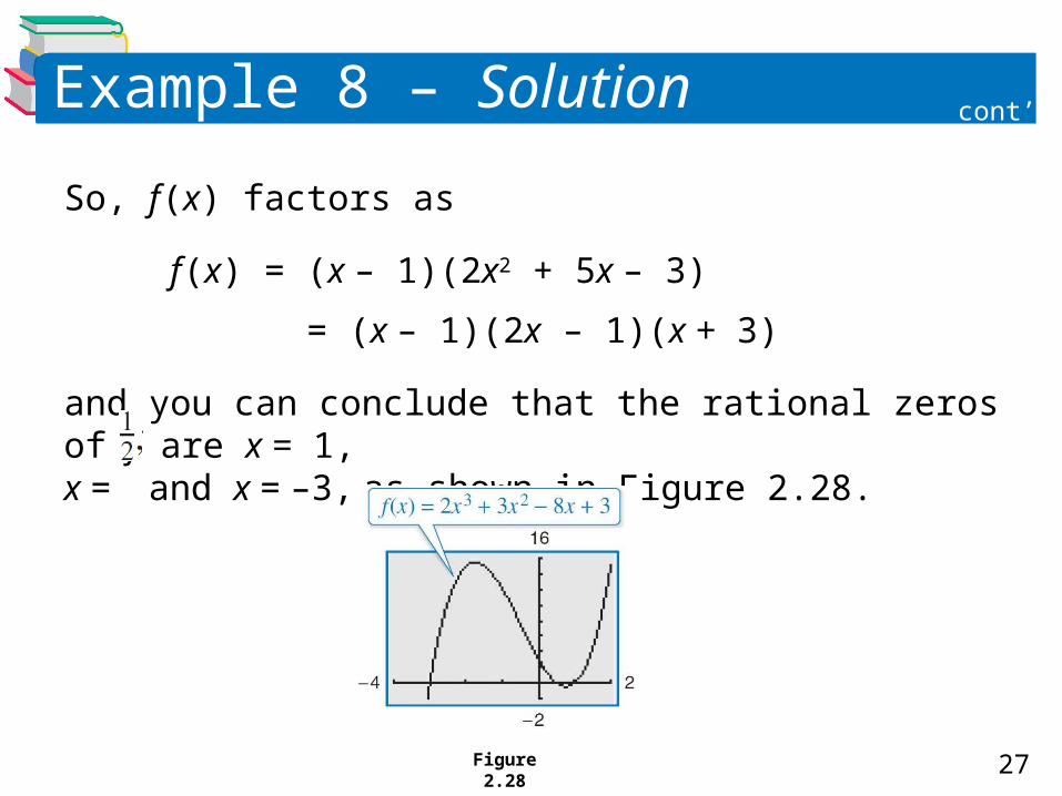
Example 8 – Solution

So, f (x) factors as

f (x) = (x – 1)(2x2 + 5x – 3)

= (x – 1)(2x – 1)(x + 3)

and you can conclude that the rational zeros of f are x = 1,x = and x = –3, as shown in Figure 2.28.

cont’d

Figure 2.28

28

Other Tests for Zeros of Polynomials

29

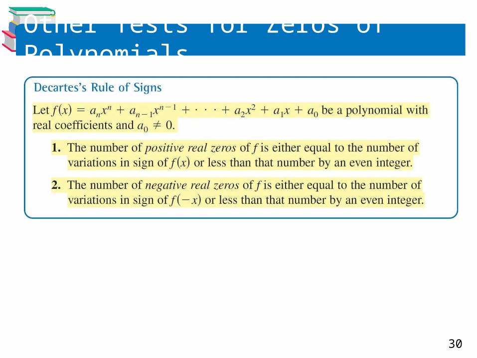
Other Tests for Zeros of Polynomials

You know that an nth-degree polynomial function can have at most n real zeros. Of course, many nth-degree polynomials do not have that many real zeros.

For instance, f (x) = x2 + 1 has no real zeros, andf (x) = x3 + 1 has only one real zero. The following theorem, called Descartes’s Rule of Signs, sheds more light on the number of real zeros of a polynomial.

30

Other Tests for Zeros of Polynomials

31

Other Tests for Zeros of Polynomials

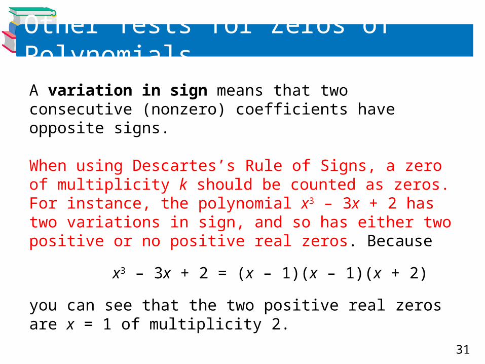
A variation in sign means that two consecutive (nonzero) coefficients have opposite signs.

When using Descartes’s Rule of Signs, a zero of multiplicity k should be counted as zeros. For instance, the polynomial x3 – 3x + 2 has two variations in sign, and so has either two positive or no positive real zeros. Because

x3 – 3x + 2 = (x – 1)(x – 1)(x + 2)

you can see that the two positive real zeros are x = 1 of multiplicity 2.

32

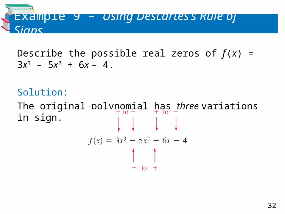
Example 9 – Using Descartes’s Rule of Signs

Describe the possible real zeros of f (x) = 3x3 – 5x2 + 6x – 4.

Solution:

The original polynomial has three variations in sign.

33

Example 9 – Solution

The polynomial

f (–x) = 3(–x)3 – 5(–x)2 + 6(–x) – 4

= –3x3 – 5x2 – 6x – 4

has no variations in sign.

So, from Descartes’s Rule of Signs, the polynomialf (x) = 3x3 – 5x2 + 6x – 4 has either three positive real zeros or one positive real zero, and has no negative real zeros.

cont’d

34

Example 9 – Solution

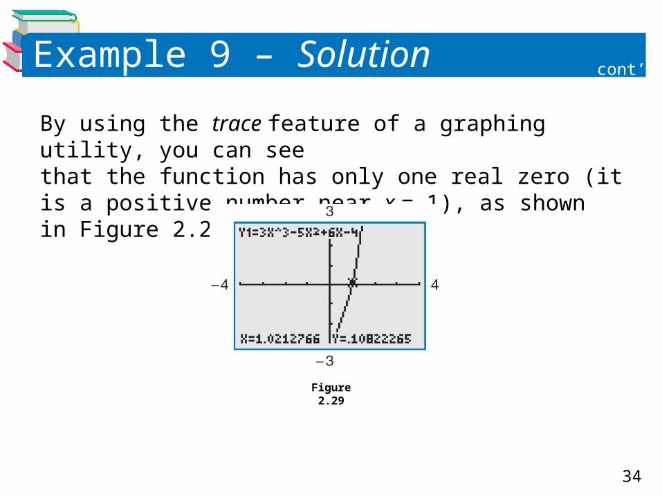
By using the trace feature of a graphing utility, you can see that the function has only one real zero (it is a positive number near x = 1), as shown in Figure 2.29.

Figure 2.29

cont’d

35

Other Tests for Zeros of Polynomials

Another test for zeros of a polynomial function is related to the sign pattern in the last row of the synthetic division array.

This test can give you an upper or lower bound of the real zeros of f, which can help you eliminate possible real zeros.

36

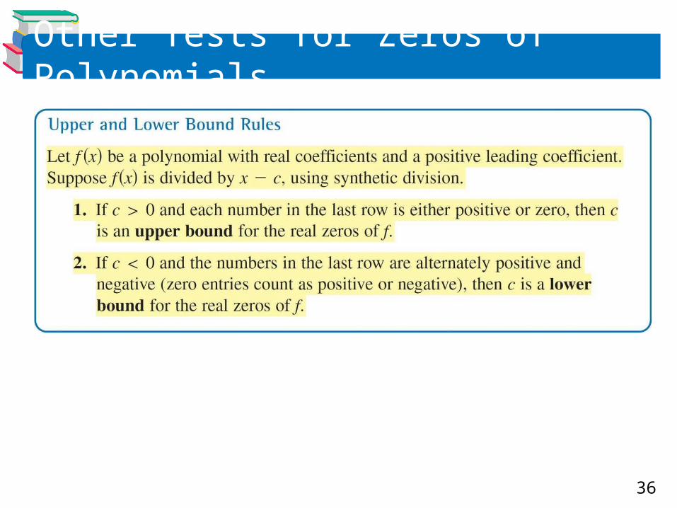
Other Tests for Zeros of Polynomials