copyright by naveen eluru · pdf filethe dissertation committee for naveen eluru certifies...
TRANSCRIPT

Copyright
by
Naveen Eluru
2010
The Dissertation Committee for Naveen Eluru certifies that this is the approved version
of the following dissertation:
Developing Advanced Econometric Frameworks for Modeling
Multidimensional Choices: An Application to Integrated Land-Use
Activity Based Model Framework
Committee:
Chandra R. Bhat, Supervisor
Randy B. Machemehl
S. Travis Waller
Stephen Donald
Sivaramakrishnan Srinivasan
Developing Advanced Econometric Frameworks for
Modeling Multidimensional Choices: An Application to
Integrated Land-Use Activity Based Model Framework
by
Naveen Eluru, B.Tech; M.S.E
Dissertation
Presented to the Faculty of the Graduate School of
The University of Texas at Austin
in Partial Fulfillment
of the Requirements
for the Degree of
Doctor of Philosophy
The University of Texas at Austin
December, 2010

Dedication
To my mother Swarajyam, my father Babu Rao, my sister Navatha
and professor B.S. Murthy

v
Acknowledgements
I was fortunate enough to meet great individuals during the course of my doctoral
education at Austin. Hence, be prepared for a long list of acknowledgements.
First and foremost, I would like to express my sincere gratitude to my advisor Dr.
Chandra R Bhat. His passion and dedication to research has and will continue to be a
source of inspiration throughout my life. I would like to thank Dr. Ram Pendyala for his
encouragement and advice. Thanks also to Dr. Travis Waller, Dr. Randy Machemehl and
Dr. Stephen Donald for serving on my dissertation committee and for other helpful
interactions. I would like to thank Siva Srinivasan, who guided me when I started my
research at UT Austin.
Professionally and personally, I would like to thank my friends Rawoof and Ipek;
Rawoof for discussions involving discrete choice models and for his constant support and
encouragement; Ipek for collaborating with me on a number of successful projects. Our
project discussions, long walks and of course her culinary skills will be missed. Other
members of my research group that I would like to thank are Rachel, Dung-Ying, Erika
and Jessica. Thanks to Lisa for the innumerable things she has helped with during the
course of my PhD.
On the personal front, I have a number of “Austinites” to thank. Pradeep and
Aswani for helping me find my feet; Vikas for cheering me up innumerable times and for
the “James Bond” car; Sudeshna for all the fun times in the basement; Aarti for all the
walks, late night ice creams and of course the arguments; Akansha for all the coffee
sessions in the basement; Nivi for speaking Telugu (albeit her version of it); Shalu for

vi
being Shalu; Deepak for innumerable visits to Mozarts and 2222 drives to discuss
problems plaguing the world; GK for being my roommate for the longest time; Shreya
and Psycho for the all night discussions; Sultana for blending so well and of course her
skillful cooking; Pondy and Rajesh for giving me company during the times I needed it
most;. Sneha for helping me embark on a journey of discovering myself and opening my
eyes to the “grey” shades in life.
I have some non-Austinite friends to thank too: Bobba for being a co-passenger in
my journey towards a PhD, Prashant for getting married first, Lava for the long
discussions and Lambu for the moral support.
I also have to thank some people who are not aware of my existence. Roger
Federer for playing tennis the only way he can; Virender Sehwag (Viru) for his simple
yet so wonderful “see ball hit ball” concept; Jon Stewart for his witty Daily Show, Ted
Dansen and Kelsey Grammer for giving me company as “Becker” and “Frasier”
respectively well after midnight.
Last, but not the least, I need to extend my thanks to my family members: my
father, my mother and my sister Navata. Without their unending trust, confidence and
support I would not be where I am today.
vii
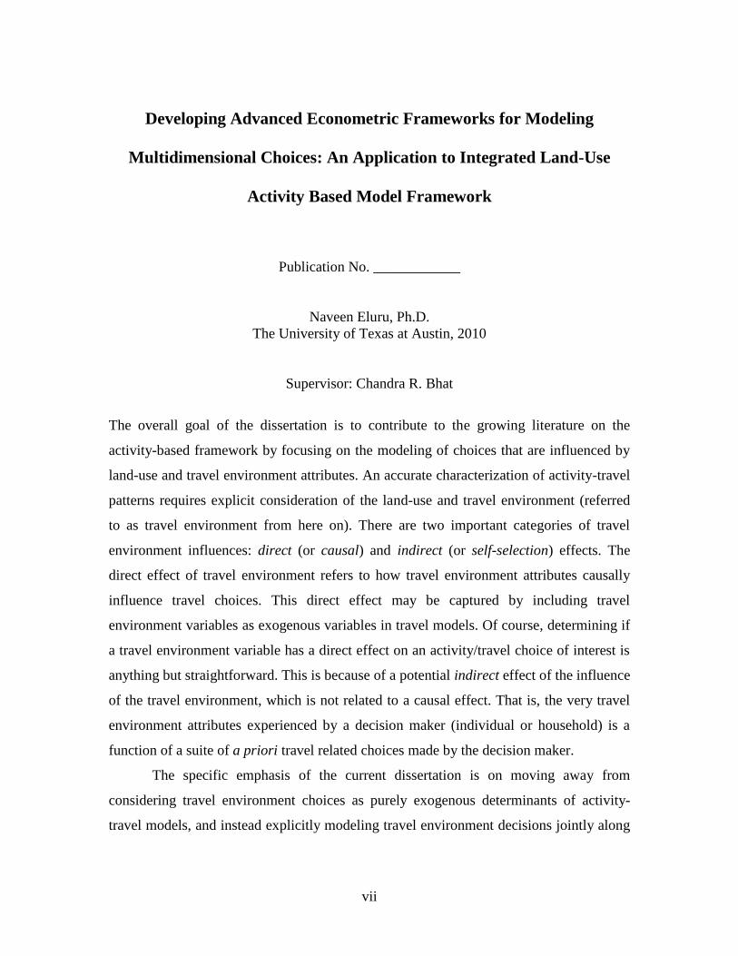
Developing Advanced Econometric Frameworks for Modeling
Multidimensional Choices: An Application to Integrated Land-Use
Activity Based Model Framework
Publication No. ____________
Naveen Eluru, Ph.D.
The University of Texas at Austin, 2010
Supervisor: Chandra R. Bhat
The overall goal of the dissertation is to contribute to the growing literature on the
activity-based framework by focusing on the modeling of choices that are influenced by
land-use and travel environment attributes. An accurate characterization of activity-travel
patterns requires explicit consideration of the land-use and travel environment (referred
to as travel environment from here on). There are two important categories of travel
environment influences: direct (or causal) and indirect (or self-selection) effects. The
direct effect of travel environment refers to how travel environment attributes causally
influence travel choices. This direct effect may be captured by including travel
environment variables as exogenous variables in travel models. Of course, determining if
a travel environment variable has a direct effect on an activity/travel choice of interest is
anything but straightforward. This is because of a potential indirect effect of the influence
of the travel environment, which is not related to a causal effect. That is, the very travel
environment attributes experienced by a decision maker (individual or household) is a
function of a suite of a priori travel related choices made by the decision maker.
The specific emphasis of the current dissertation is on moving away from
considering travel environment choices as purely exogenous determinants of activity-
travel models, and instead explicitly modeling travel environment decisions jointly along
viii
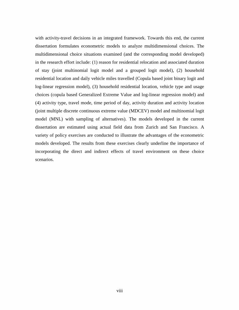
with activity-travel decisions in an integrated framework. Towards this end, the current
dissertation formulates econometric models to analyze multidimensional choices. The
multidimensional choice situations examined (and the corresponding model developed)
in the research effort include: (1) reason for residential relocation and associated duration
of stay (joint multinomial logit model and a grouped logit model), (2) household
residential location and daily vehicle miles travelled (Copula based joint binary logit and
log-linear regression model), (3) household residential location, vehicle type and usage
choices (copula based Generalized Extreme Value and log-linear regression model) and
(4) activity type, travel mode, time period of day, activity duration and activity location
(joint multiple discrete continuous extreme value (MDCEV) model and multinomial logit
model (MNL) with sampling of alternatives). The models developed in the current
dissertation are estimated using actual field data from Zurich and San Francisco. A
variety of policy exercises are conducted to illustrate the advantages of the econometric
models developed. The results from these exercises clearly underline the importance of
incorporating the direct and indirect effects of travel environment on these choice
scenarios.
ix
Table of Contents
LIST OF FIGURES ....................................................................................................... xiv
LIST OF TABLES .......................................................................................................... xv
CHAPTER 1 INTRODUCTION ............................................................................... 1
1.1 Auto-oriented travel in the United States ........................................................ 1
1.2 Activity-based travel modeling framework ..................................................... 2
1.3 Conceptual overview of activity-based framework ........................................ 4
1.3.1 Disaggregate level individual and household attribute generator (DIHG) .... 5
1.3.2 Demographic, land-use and travel environment attribute generator
(DLUTEG) ................................................................................................................... 5
1.3.3 Activity travel pattern attribute generator (ATPG) ........................................ 7
1.3.4 Traffic assignment (TA) ................................................................................ 8
1.3.5 Iterative procedure ......................................................................................... 9
1.4 Focus of current research effort ..................................................................... 10
1.4.1 Role of land-use and travel environment ..................................................... 10
1.4.2 The current study in the context of direct and indirect travel environment
effects ...................................................................................................................... 11
1.5 Objectives of the dissertation .......................................................................... 12
1.6 Structure of the dissertation ........................................................................... 14
CHAPTER 2 MODELING HOUSEHOLD RESIDENTIAL RELOCATION
DECISIONS ............................................................................................................. 20
2.1 Background ...................................................................................................... 20
x
2.2 Literature review ............................................................................................. 21
2.3 Focus of current chapter ................................................................................. 23
2.4 Modeling methodology .................................................................................... 26
2.5 Empirical analysis ............................................................................................ 30
2.5.1 Data Source .................................................................................................. 30
2.5.2 Sample preparation ...................................................................................... 30
2.5.3 Model structures estimated .......................................................................... 32
2.5.4 CRMO model estimation results .................................................................. 33
2.5.5 Model assessment ........................................................................................ 37
2.6 Summary ........................................................................................................... 37
CHAPTER 3 EXAMINING THE INFLUENCE OF BUILT ENVIRONMENT
ON TRAVEL DEMAND ................................................................................................ 42
3.1 Introduction ...................................................................................................... 42
3.1.1 Semi-Parametric and Non-Parametric Approaches ..................................... 45
3.1.2 The Copula Approach .................................................................................. 46
3.2 Overview of the copula approach ................................................................... 47
3.2.1 Background .................................................................................................. 47
3.2.2 Copula Properties and Dependence Structure.............................................. 49
3.2.3 Alternative Copulas ..................................................................................... 53
3.3 Model estimation and measurement of treatment effects ............................ 60
3.3.1 Maximum Likelihood Estimation ................................................................ 61
3.4 Data ................................................................................................................... 62
3.4.1 Data sources ................................................................................................. 62
xi
3.4.2 The Dependent Variables ............................................................................. 63
3.5 Empirical analysis ............................................................................................ 64
3.5.1 Variables considered .................................................................................... 64
3.5.2 Estimation Results ....................................................................................... 64
3.6 Summary ........................................................................................................... 68
CHAPTER 4 HOUSEHOLD VEHICLE FLEET COMPOSITION AND USAGE
CHOICES ............................................................................................................. 74
4.1 Introduction and literature ............................................................................. 74
4.2 Modeling methodology .................................................................................... 76
4.2.1 Model framework......................................................................................... 76
4.2.2 Model Structure ........................................................................................... 79
4.2.3 Model estimation ......................................................................................... 83
4.3 Data ................................................................................................................... 85
4.3.1 Sample characteristics .................................................................................. 86
4.4 Empirical analysis ............................................................................................ 87
4.4.1 Model Estimation Results ............................................................................ 89
4.4.2 Model Assessment ....................................................................................... 92
4.5 Summary ........................................................................................................... 94
CHAPTER 5 ACTIVITY PARTICIPATION DECISIONS ............................... 101
5.1 Introduction and motivation ......................................................................... 101
5.1.1 Joint model systems ................................................................................... 102
5.1.2 Current research effort ............................................................................... 103
5.2 Modeling methodology .................................................................................. 105
xii
5.2.1 Utility Structure ......................................................................................... 105
5.2.2 Econometric Structure ............................................................................... 108
5.2.3 Sampling of Location Choice Alternatives ................................................ 110
5.2.4 An Intuitive Behavioral Interpretation ....................................................... 112
5.3 Data Description............................................................................................. 113
5.4 Empirical analysis .......................................................................................... 114
5.4.1 Model specification and estimation ........................................................... 114
5.4.2 Model assessment ...................................................................................... 115
5.4.3 Estimation results ....................................................................................... 116
5.5 Summary ......................................................................................................... 118
CHAPTER 6 POLICY ANALYSIS ...................................................................... 124
6.1 Background .................................................................................................... 124
6.2 Household residential relocation decision ................................................... 125
6.2.1 Elasticity effects computation .................................................................... 125
6.2.2 Elasticity effects ......................................................................................... 127
6.3 Residential location and VMT ...................................................................... 128
6.3.1 Treatment Effects ....................................................................................... 130
6.3.2 Treatment effect results.............................................................................. 132
6.4 Household vehicle fleet composition and usage choices ............................. 135
6.4.1 Policy exercise ........................................................................................... 135
6.4.2 Results ........................................................................................................ 135
6.5 Activity participation decisions .................................................................... 137
6.5.1 Policy exercise details ................................................................................ 137
6.5.2 Policy exercise results ................................................................................ 138
xiii
6.6 Summary ......................................................................................................... 139
CHAPTER 7 CONCLUSIONS AND DIRECTIONS FOR FURTURE
RESEARCH ........................................................................................................... 145
7.1 Introduction .................................................................................................... 145
7.2 Household residential relocation decision ................................................... 146
7.3 Residential location and VMT ...................................................................... 148
7.4 Household vehicle fleet composition and usage choices ............................. 149
7.5 Activity participation decisions .................................................................... 150
7.6 Directions for future research....................................................................... 151
7.6.1 Limitations ................................................................................................. 151
7.6.2 Research extensions ................................................................................... 152
APPENDIX 1 ........................................................................................................... 154
REFERENCES ........................................................................................................... 155
VITA ........................................................................................................... 167

xiv
LIST OF FIGURES
Figure 1.1: Conceptual representation of activity-based modeling framework. ............... 16
Figure 1.2: A schematic representation of the dissertation ............................................... 17
xv
LIST OF TABLES
Table 1.1: Activity-based modeling frameworks .............................................................. 18
Table 1.2: Demographic, land-use and travel environment attribute generator (DLUTEG)
evolution component modules .......................................................................................... 19
Table 2.1: Sample Characteristics ..................................................................................... 39
Table 2.2: Reason to Move Component of Joint Model ................................................... 40
Table 2.3: Duration of Stay Component of Joint Model .................................................. 41
Table 3.1: Characteristics of Alternative Copula Structures ............................................ 71
Table 3.2: Expressions for 1 2
2
( , )C u uu
........................................................................ 72
Table 3.3: Estimation Results of the Switching Regime Model ....................................... 73
Table 4.1: Sample Characteristics .................................................................................... 97
Table 4.2: Frank Copula Model Results: MNL component ............................................ 98
Table 5.1: Descriptive Statistics of Activity participation and Time-Use by Activity
Purpose, Activity Timing and Travel mode .................................................................... 120
Table 5.2: The MDCEV Model Results: Baseline Parameter Estimates ........................ 121
Table 5.3: MNL Component (Location Choice) Model Estimation Results .................. 123
Table 6.1: Elasticity Values for the Move Reason Choice ............................................. 140
Table 6.2: Elasticity Values for the Duration of Stay Choice......................................... 141
Table 6.3: Estimates of Treatment Effects in Miles ....................................................... 142
Table 6.4: Model Application ........................................................................................ 143
Table 6.5: Policy Simulation Results .............................................................................. 144
1
CHAPTER 1 INTRODUCTION
1.1 Auto-oriented travel in the United States
In the United States, a significant number of individuals depend on the auto mode of
transportation. This dependency on the auto mode can be attributed to high
auto-ownership affordability, inadequate public transportation facilities (in many cities),
and excess suburban land-use developments. For instance, the 2009 NHTS data shows
that about 91% of US households owned at least one motor vehicle in 2009 (compared to
about 80% in the early 1970s; see Pucher and Renne, (2003)). The high auto dependency,
in turn, results in high auto travel demand on highways. At the same time, the ability to
build additional infrastructure is limited by high capital costs, real-estate constraints and
environment considerations. The net result has been that traffic congestion levels in
metropolitan areas of United States have risen substantially over the past decade (see
Schrank and Lomax, (2005)). The increase in traffic congestion levels not only causes
increased travel delays and impacts stress levels of drivers, but also adversely affects the
environment as a result of rising air pollution and green house gas emissions.
To be sure, the past few decades have seen considerable progress in automobile
technology, leading to a reduction in the amount of pollutants released into the
environment and an increase in the mileage per gallon of gasoline used (Foundation for
Clean Air Progress (FCAP)). For example, on average, about 20 of today‟s cars put
together produce the same amount of per-mile emissions as one mid-1960s car. In
another 10 years, thanks to new automotive and fuel technologies, it is expected that 33
cars will produce the same amount of per-mile emissions as one of mid-1960s model (Air
pollution facts, FCAP). However, the advantages of the progress in the automobile
industry are offset considerably by the escalated ownership of personal automobiles and
their subsequent use for work and non-work trips. The household vehicle miles of travel
increased 300% between 1977 and 2001 (relative to a population increase of 30% during
the same period; see Polzin et al., (2004)). The increasing vehicle miles traveled has
resulted in an increase in the quantity of emissions in recent years. In fact, in many urban
2
regions, the quantity of emissions is very close to the threshold or beyond the threshold of
the Environmental Protection Agency (EPA) conformity levels. Of course, these mobile-
source emissions in the environment also contribute to global warming (Greene and
Shafer, (2003)).
The increasing auto travel, and its adverse environmental impacts, has led, in the
past decade, to the serious consideration and implementation of travel demand
management (TDM) strategies (for example, promoting car sharing schemes, enhancing
existing public transportation services and building new services such as light rail
transit). The main objective of these TDM strategies is to encourage the efficient use of
transportation resources by influencing travel behavior. TDM strategies offer flexible
solutions that can be tailored to meet the specific requirements of a particular urban
region. Concomitant with this emphasis on demand management has been the stronger
emphasis on analyzing traveler behavior at the individual level rather than using direct
statistical projections of aggregate travel demand. In particular, the focus of travel
demand modeling has shifted from an underlying trip-based paradigm to an activity-
based paradigm, which treats travel as a demand derived from the need to participate in
activities dislocated in time and space (see Bhat and Koppelman, (1993)). This activity-
based paradigm is discussed in more detail in the rest of this chapter, along with the
objectives of this dissertation.
The remainder of this chapter is organized as follows. Section 1.2 provides a brief
summary of activity-based travel models, while Section 1.3 presents an overview of a
typical activity-based modeling framework. In Section 1.4 we discuss the focus of the
current research and outline the importance of land-use and travel environment in
modeling activity patterns. Section 1.5 presents the objectives of the dissertation. Section
1.6 outlines the rest of the dissertation.
1.2 Activity-based travel modeling framework
The objective of an activity-based travel modeling framework is to micro-simulate
individual activity and travel participation over the course of certain time interval, which
3
usually is a typical weekday. The framework considers travel as a means to pursue
activities distributed in time and space. The activity-based modeling framework
essentially attempts to replace the statistical travel prediction focus of the traditional trip-
based model framework with a more behavioral approach that explicitly recognizes the
fundamental role of activity participation as a precursor to travel. In doing so, the
activity-based framework offers several advantages from a travel modeling perspective.
First, it ensures that there is consistency across the different choices (for example, mode
choices, time-of-day choices, and destination choices) assigned to successive trips of an
individual. Second, the modeling of daily patterns allows a more accurate analysis of the
changes to travel patterns in response to travel demand management strategies and policy
initiatives, because of the explicit recognition of the interplay among the several activity
participation-related choices of an individual. Third, the activity-based models allow the
incorporation of the influence of inter-household interactions on travel. Finally the
activity-based framework generally considers a finer resolution of time and space
(compared to the traditional trip-based framework), and thus is more suited to providing
travel inputs needed for vehicle emissions and air quality modeling.
To better illustrate the advantages of the activity-based modeling framework,
consider an employer-based work policy that involves releasing employees early from
work in the afternoon to reduce PM peak period traffic. Since there is little to no
connection between the prediction of work trips and non-work trips in the trip-based
framework, the use of a trip-based approach may lead one to believe that the employer
work policy would indeed reduce trips in the PM peak. However, from an activity
participation standpoint, it is possible that individuals use the additional time available
now in the late afternoon to pursue more non-work activities during evening commute or
after returning home. If some of these “new” non-work activity participations are pursued
during the peak period, the reduction in peak period trips, as predicted by an activity-
based modeling framework, will be lesser than predicted by the trip-based framework.
Previous studies have clearly indicated such an “available time” effect on the generation
of non-work activities (see Bhat et al., 2004), which implies that the trip-based
4
framework can over-predict the benefit of an “early-release-from-work” policy, while the
activity-based framework provides more realistic responses.
Federal transportation agencies and metropolitan organizations (MPOs) in the
United States and Europe have started to recognize the advantages of the activity-based
framework and are investing substantially in the development and deployment of
activity-based models. Examples of urban regions in the United States and Europe that
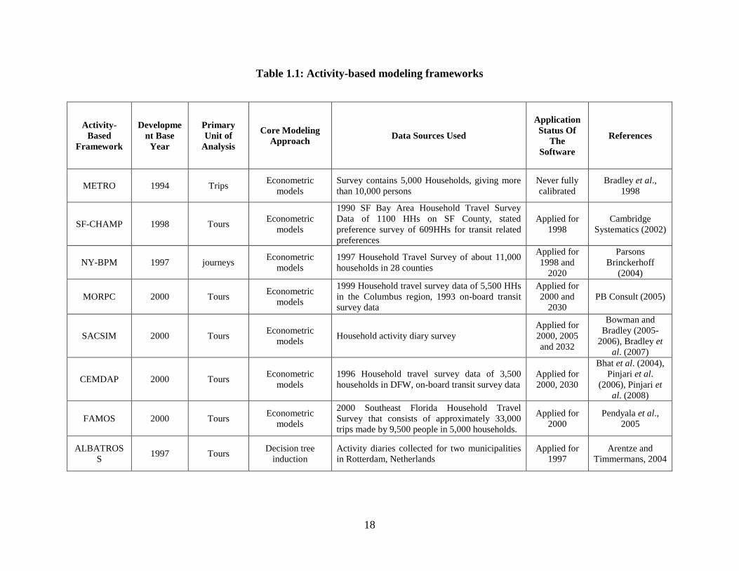
have an operational or research based activity model include (name of the software in
parenthesis): Portland (METRO), San Francisco (SF-CHAMP), New York (NY-BPM),
Columbus (MORPC), Sacramento (SACSIM), Dallas-Fort-Worth (CEMDAP), Southeast
Florida (FAMOS), and Rotterdam (ALBATROSS). A brief review of these models is
provided in Table 1.1. Specifically, the table presents details of the development base
year, the primary unit of analysis, the core modeling approach, the data sources used, the
application status of the software and references. All the frameworks discussed in the
table employ microsimulation for generating travel forecasts.
1.3 Conceptual overview of activity-based framework
In this section, we provide a conceptual overview of an activity-based modeling
framework. A schematic description provided in Figure 1.1 identifies the following key
elements: (1) disaggregate level individual and household attribute generator (DIHG), (2)
demographic, land-use and travel environment attribute generator (DLUTEG), (3)
activity travel pattern attribute generator (ATPG), and (4) traffic assignment module
(TA). The schematic also outlines the base year inputs typically provided for activity-
based models, which include information on the aggregate socioeconomics and the
activity-travel environment characteristics in the urban study region for the base year, as
well as policy actions prescribed for future years.
In the subsequent discussion, we present details of how each of the different
elements identified above operate within an iterative procedure to generate activity travel
patterns for the forecast year.
5
1.3.1 Disaggregate level individual and household attribute generator (DIHG)
The activity-based modeling frameworks employ disaggregate level individual and
household level information to model activity-travel patterns. The DIHG element is also
often referred to as synthetic population generation with the travel demand community.
The DIHG generation involves an aggregate dataset that represents the desired or
expected marginal distribution of the variables (such as Summary Files (SF) of the U.S.
or the Small Area Statistics (SAS) files of the U.K) and a disaggregate dataset that is a
collection of records representing a sample of the “real” households and individuals in
the population (for example Public-Use Microdata Samples (PUMS) of the U.S. and the
Sample of Anonymized Records (SAR) of the U.K). The disaggregate population
attributes are generated by selecting records from the disaggregate dataset while ensuring
that the marginal distributions from the aggregate dataset match using an Iterative
Proportional Fitting (IPF) approach or its variants. The marginal distributions selected for
the matching process form the control totals for the synthetic population generation.
Typically, researchers employ a sub-set of person (such as age, gender and race) and
household (such as head of the household age, and household size) attributes as control
variables (see Guo and Bhat 2007 and Xin et al., 2009 for more details on DIHG
procedures). The data generated based on these control totals in the DIHG module
contains details of all person and household attributes. However, because we employ only
some dimensions as control variables in the data generation, the “un-controlled” variable
information is typically removed from the data set and re-generated using the DLUTEG
element. It is important to note that DIHG procedure is only employed at the beginning of
the first iteration. Subsequently, the procedure iterates between DLUTEG, ATPG and TA
elements.
1.3.2 Demographic, land-use and travel environment attribute generator
(DLUTEG)
Recent literature in travel demand modeling community has emphasized the importance
of generating accurate land-use and travel environment attributes for improving activity-
6
based travel forecasting (see Bhat and Guo 2007, Pinjari et al., 2009 for a detailed
discussion). The DLUTEG element generates disaggregate level land-use and travel
environment information for all individuals in the DIHG synthesized population. The
DLUTEG element, typically, consists of two components: (1) base year component and
(2) an evolution component.
1.3.2.1 Base year component
The major function of the base year component is to augment the available demographic
variables with other relevant variables required for activity travel pattern generation.
These variables generally include: study status, labor participation, employment location,
employment schedule, employment flexibility at the individual level, household income,
residential tenure, housing type, vehicle ownership, and vehicle fleet composition at the
househol level1. These variables are generated using a series of sequential modules, all
embedded within a microsimulation platform. Typically, all the person-related variables
are generated first, and appropriately aggregated to compute such household level
attributes as household income, number of workers, followed by the generation of other
household level attributes (see Eluru et al., 2007).
1.3.2.2 Evolution component
The base year component of the DLUTEG model is adequate if the emphasis is on
generating travel patterns solely for the base year. However, the objective of most
transportation planning exercises is to forecast forward into a future year, or to examine
the travel impact of policy changes related to the transportation system. In such predictive
contexts, there is a need to explicitly model how the individuals, households, land-use
forms and the travel environment evolve over time. The choices typically modeled in the
evolution components include: (1) individual-level evolution and choice models (for
1 The household residential location determination for the base year is typically made within the DIHG
element..
7
births, deaths, schooling, and employment) (2) household formation models (for living
arrangement, divorce, move-ins, and move-outs from a family), (3) household-level long-
term choice models (for residential moves, duration of stay, residential housing
characteristics, automobile fleet composition, annual automobile usage, information and
communication technology adoption, and bicycle ownership) and (4) land-use policies (to
represent urban form regulations and firm establishment and relocation decisions). The
evolution components also typically employ an a priori sequential structure for modeling
the choices identified.
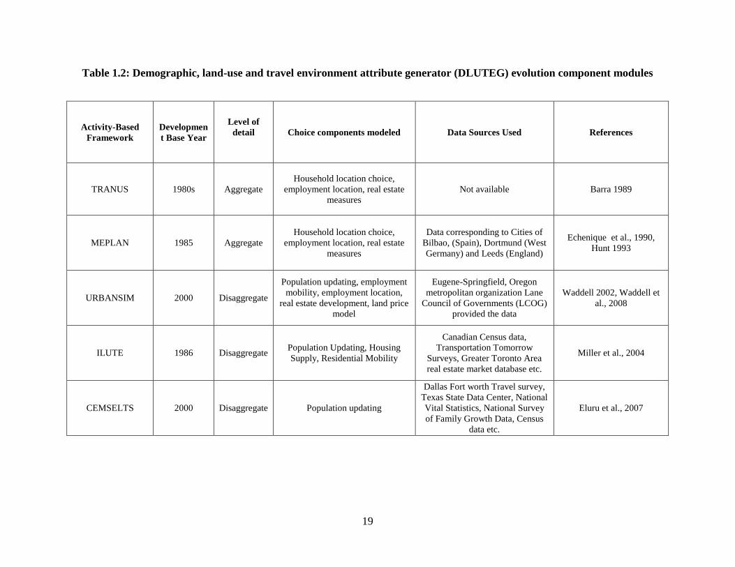
To date, a number of demographic and socioeconomic updating modules have
been developed in the field of sociology (for example DYNAMOD, DYNACAN,
NEDYMAS, and LIFEPATHS). These modules explicitly model demographic processes
at a high level of detail. However, they are not well suited for application in the context
of an activity-based travel microsimulation system because generating the necessary
land-use and transportation system characteristics required for an activity-based travel
microsimulator with these models is not straightforward. Examples of population and
land-use updating systems that have been developed in the travel demand forecasting
community (and with varying levels of detail and sophistication) include TRANUS,
MEPLAN, URBANSIM, ILUTE, and CEMSELTS. Table 1.2 provides a brief summary
of the aforementioned systems with brief details regarding the base year of development,
level of detail of information, choice components modeled, data sources used and
references.
1.3.3 Activity travel pattern attribute generator (ATPG)
The third element of the activity based model is the activity travel pattern attribute
generator. The ATPG employs the outputs from the DLUTEG element to predict activity
travel patterns for the entire population in the urban region. This activity-based micro-
simulation effort, in addition to determining the different activities pursued, involves,
among other things, modeling activity location, activity duration, individuals
participating in the activity, and the travel mode (for out-of-home activities) to the
8
activity2. In determining these choices, the ATPG considers a host of factors including:
(1) individual socio-demographics (such as age, gender, race, employment status,
employment location), (2) household socio-demographics (such as number of household
members, number of children, number of employed individuals, household location, and
vehicle fleet composition and usage), and (3) the travel environment (level of service
(LOS) measures such as travel time to location, accessibility to activity locations,
perception of space, time of day, access to vehicles, access to public transportation, and
presence of bicycling and walking infrastructure). The information regarding these
factors is obtained from the outputs generated from the DIHG and DLUTEG components
of the framework. The DLUTEG and ATPG components require LOS measures for the
transportation network. For this purpose, an initial set of LOS measures is assumed for
the first iteration. These LOS measures are updated based on the LOS measures
generated in the traffic assignment (TA) module.
1.3.4 Traffic assignment (TA)
Recent advances in integrating activity based models with advanced assignment
methodologies enable us to directly translate, based on continuous time intervals, the
activity-travel patterns generated from the ATPG into vehicles on the transportation
network. To elaborate, the activity-travel patterns generated are converted into dynamic
origin destination (O-D) matrices (see Lin et al., 2008) that are then input to the TA
module. Within the TA module, the network assignment undertakes traffic simulation,
optimal routing and path assignment to obtain traffic link volumes and speeds. The travel
times obtained as outputs from the TA module are appropriately processed and provided
as input back to DLUTEG and ATPG element. Then the DLUTEG and ATPG elements
2 The actual attributes modeled in the ATPG vary based on the implementation instance developed for
micro-simulation. For instance, tour models do not explicitly model activity durations in their effort to
mimic individuals‟ activity participation.
9
are re-run to generate revised outputs. This “within year” iteration is continued until there
is little change in the convergence criterion3.
1.3.5 Iterative procedure
The preceding discussion presented the details of one time-step in the activity-based
framework. In the next phase of the activity-based framework in Figure 1.1, the emphasis
on moving one step forward in time (usually this step is considered as one year), by
updating the population, urban-form, and the land-use markets, using the evolution
component of the DLUTEG element (note that the DIHG is used only to generate the
disaggregate-level synthetic population for the base-year and is not used beyond the base
year). An initial set of transportation system attributes is generated for this next time step
based on (a) the population, urban form, and land-use markets for the next time step, (b)
the transportation system attributes from the previous year in the simulation, and (c) the
future year policy scenarios provided as input. The DLUTEG element outputs are then
provided as input into ATPG, which interfaces with a TA element in a series of
consistency/equilibrium iterations for the next time step (just as for the base year) to
obtain the “one time step” outputs. The loop continues for several time steps forward
until the socioeconomics, land-use, and transportation system path/link flows and
transportation system level of service are obtained for the forecast year specified by the
analyst.
3 Two possible convergence criteria have been used in literature: (1) O-D matrix convergence and (2) travel
time convergence. In the former, the O-D trip tables generated in the current iteration are checked against
the O-D trip values generated in the previous iteration. If the O-D matrices are within a certain tolerance,
the iterations are terminated and the O-D matrices with the corresponding link volumes and speeds are
provided for analysis. The travel time convergence criterion is similar, except that the link travel times
predicted in the current iteration are checked against corresponding values in the previous iteration. If these
are within a certain tolerance, convergence is assumed to have been reached.
10
1.4 Focus of current research effort
In the preceding section, we discussed a “blueprint” of an activity-based model
framework and briefly summarized how the many elements of the framework interact
with one another. The overall goal of the dissertation is to contribute to this growing
literature on the activity-based framework by focusing on the modeling of choices that
are influenced by land-use and travel environment attributes. These choices fall within
the realm of the DLUTEG and ATPG components of the framework of Section 1.3.
1.4.1 Role of land-use and travel environment
An accurate characterization of activity-travel patterns requires explicit consideration of
the land-use and travel environment (referred to as travel environment from here on).
There are two important categories of travel environment influences: direct and indirect
effects. The direct effect of travel environment refers to how travel environment
attributes causally influence travel choices. This direct effect may be captured by
including travel environment variables as exogenous variables in travel models. For
example, a household‟s residential location may affect the travel mode choice for activity
participation of each of the household members. If the household resides in a suburban
region with inadequate public transportation service it is likely that members of the
household will pursue activities using the auto mode. This may be captured by
incorporating, for instance, residential location-related public transportation accessibility
measures in a travel mode choice model. Other similar accessibility measures may
include length/density of bicycle (highway) lanes within a mile radius of the household,
and accessibility to shopping, recreation or maintenance activities by alternate modes. If
such direct measures turn out to be statistically significant predictors of activity-travel
choices, the suggestion is that transportation decision-makers may be able to influence
activity/travel choices by making appropriate design changes to the travel environment.
For instance, the growing environmental and public health concerns have led to studies
that attempt to examine if and how altering travel environment (densification of
11
neighborhoods, improving bicycling facilities etc.) results in changes to walking and
transit-use behavior.
Of course, determining if a travel environment variable has a direct effect on an
activity/travel choice of interest is anything but straightforward. This is because of a
potential indirect effect of the influence of the travel environment, which is not related to
a causal effect. That is, the very travel environment attributes experienced by a decision
maker (individual or household) is a function of a suite of a priori travel related choices
made by the decision maker. For instance, a decision maker who has an intrinsic
preference for driving may not mind residing in a suburban region of the metropolitan
area with minimal transit accessibility. On the other hand, a decision maker who is
“environmentally conscious” might possibly choose to reside in a downtown region of
the metropolitan area, so that s/he can use public transportation for a large fraction of
her/his travel. In both cases, the decision maker chooses a travel environment that would
be conducive to a priori travel dispositions. In the context of the above example, if we
disregard that residential location is a choice (i.e. if we ignore that decision makers may
self-select their residential location), the analysis results may suggest incorrectly that
creating dense neighborhoods will substantially reduce vehicular usage (mileage). This is
not to say that policies that alter travel environment are generically ineffectual, but that
the emphasis needs to be on carefully disentangling the direct (or causal) and indirect
(self-selection) influence of the travel environment on activity/travel choices.
1.4.2 The current study in the context of direct and indirect travel environment
effects
The emphasis of the current dissertation is on moving away from considering
travel environment choices as purely exogenous determinants of activity-travel models,
and instead explicitly modeling travel environment decisions jointly along with activity-
travel decisions in an integrated framework. In the example discussed in the previous
section, this would mean jointly modeling residential choice decisions along with travel
mode choice dimensions, and accommodating the effects of individual pre-dispositions
12
(such as auto-inclination or environment-friendliness) on both residential and travel
choices. Once this indirect (or spurious or self-selection) effect is captured, the remaining
effect of the travel environment on travel choice may be more realistically considered as
the “true” (or direct or causal) effect. Of course, the example provided in the previous
section is but one of the many potential joint choices within the gamut of choices in
DLUTEG and ATPG. Other possible joint choice situations (within the DLUTEG and
ATPG components) likely to manifest direct and indirect travel environment effects
include: (1) reason for residential relocation and associated duration of stay, (2)
household residential location and vehicle ownership, (3) household residential location
and daily vehicle miles travelled, (4) household residential location, vehicle type and
usage choices, (5) activity type, travel mode, time period of day, activity duration and
activity location. There is a need to develop econometric models that can potentially
model such multidimensional choices (see Pinjari et al., 2007 and Bhat and Guo, 2007 for
examples of earlier studies along these lines). In this dissertation, we contribute
substantively to the development of such multidimensional choice models of travel
environment and activity-travel choices, while also addressing several methodological
challenges, in doing so, as discussed next.
1.5 Objectives of the dissertation
Recent research in activity-based models has called for the unification of different
streams of research on transportation planning, land-use modeling and activity time-use.
This is, at least in part, to disentangle causal (or direct) effects of travel environment
variables from spurious (or self-selection or indirect) effects (see Cao et al., 2008, and
Pinjari, 2009). The current dissertation contributes to this existing research by (a)
developing advanced econometric models for modeling multi-dimensional choices, (b)
estimating these models for travel data sets, and (c) undertaking policy analysis.
The specific objectives of the current dissertation are four fold as discussed in
more detail below:
13
The first objective is to contribute substantively to the growing stream of literature on
multidimensional choices within an integrated land-use activity-based model framework.
Specifically, the multidimensional choice situations examined in the research effort
include: (1) reason for residential relocation and associated duration of stay, (2)
household residential location and daily vehicle miles travelled, (3) household residential
location, vehicle type and usage choices and (4) activity type, travel mode, time period of
day, activity duration and activity location.
The second objective is to formulate a suite of econometric models that are applicable to
examine the different multi-dimensional choice contexts identified above. Specifically,
the econometric models developed, in sequence of the choice contexts mentioned earlier,
include: (1) joint multinomial logit model and a grouped logit model, (2) Copula based
joint binary logit and log-linear regression model, (3) copula based Generalized Extreme
Value and log-linear regression model, and (4) joint multiple discrete continuous extreme
value (MDCEV) model and multinomial logit model (MNL) with sampling of
alternatives.
The third objective is to apply the multidimensional choice model formulations in an
actual field context to understand the direct and indirect effects of travel environment
variables on activity-travel choices. We do so by using activity-travel surveys conducted
in two urban regions in the world. These correspond to (1) a longitudinal data set derived
from a retrospective survey that was administered in the beginning of 2005 to households
drawn from a stratified sample of municipalities in the Zurich region of Switzerland and
(2) a cross-section two-day retrospective activity survey travel data set derived from the
2000 San Francisco Bay Area Household Travel Survey (BATS). The Zurich dataset is
employed for modeling residential moves and duration of stay while the BATS data is
employed for the other three multidimensional choices.
14
The fourth objective is to undertake validation and policy analysis, relevant to the choice
context under consideration, to clearly examine the advantages of modeling these choices
as multidimensional choices as opposed to considering them as sequential choices.
1.6 Structure of the dissertation
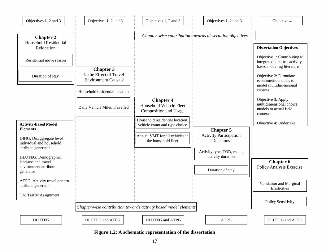
Figure 1.2 presents a schematic representation of the structure of the remainder of the
dissertation, which shows how each chapter contributes to the activity-based model
components identified in Section 1.3 and how each chapter furthers the objectives of the
dissertation. Within each chapter, an exhaustive literature review is conducted to discuss
earlier research, identify limitations of earlier research, and position the research effort in
the current dissertation within the larger context of the literature.
Chapter 2 examines the household residential relocation decision at the household
level, both in terms of the reasons for relocation and in terms of the duration of stay at a
given residential location. The joint modeling of the move decision and the stay duration
is important because they are simultaneous decisions in the sense of being
contemporaneous i.e. the move decision and the stay duration represent a package choice.
The model takes the form of a joint multinomial logit model of reason for move and a
grouped logit model of residential stay duration preceding the move.
Chapter 3 addresses the following question: Is the effect of the built environment
on travel demand causal or merely associative or some combination of the two? Towards
this end, a model of residential neighborhood choice and daily household vehicle miles of
travel (VMT) is formulated. The dominant approach in the literature to dealing with such
self-selection choice situations is to assume a bivariate normality assumption directly on
the error terms, or on transformed error terms, in the discrete neighborhood choice and
continuous VMT equations. Such an assumption can be restrictive and inappropriate,
since the implication is a linear and symmetrical dependency structure between the error
terms. In this dissertation, we introduce and apply a flexible approach to sample selection
in the context of built environment effects on travel behavior. The approach is based on
the concept of a “copula”, which is a multivariate functional form for the joint
15
distribution of random variables derived purely from pre-specified parametric marginal
distributions of each random variable. The copula-based approach retains a parametric
specification for the bivariate dependency, but allows testing of several parametric
structures to characterize the dependency.
Chapter 4 focuses on modeling household vehicle fleet composition and usage
choices, which include the household vehicle count, vehicle type (classified as small
sedan, large sedan, coupe, van, pick-up truck and sports utility vehicle), and annual
vehicle usage decisions. However, the framework needs to take into account the impact
of residential self-selection effects on vehicle fleet composition and usage. To do so, the
chapter presents a joint GEV-based logit regression model of residential location choice,
vehicle count by type choice, and vehicle usage (vehicle miles of travel) using a copula
based framework that facilitates the estimation of joint equations systems with error
dependence structures within a simple and flexible closed-form analytic framework.
Chapter 5 examines activity participation decisions in a unified framework that
simultaneously determines activity type choice (generation), time of day choice, mode
choice, destination choice, and time use allocation (duration). The unified framework
allows us to capture the effects of spatial land use and built environment characteristics
on activity generation, an effect often incorporated in a very tedious cascading fashion in
earlier literature. The model system formulated constitutes a joint multiple discrete
continuous extreme value (MDCEV) – multinomial logit (MNL) model, in which all
discrete choices except for destination choice as well as the continuous duration
dimension are modeled using the MDCEV, while destination choice is modeled as a
MNL (with sampling of alternatives) nested and integrated within the MDCEV model
component.
Chapter 6 undertakes validation and policy evaluation exercises for the
econometric models developed in Chapters 2 through 5.
Chapter 7 discusses the substantive implications of the policy exercises for
informed policy making. The chapter also identifies future directions of research and
concludes the dissertation.

16
Figure 1.1: Conceptual representation of activity-based modeling framework.
Activity-travel
environment
characteristics
(base year)
Policy actions
Aggregate
socioeconomics
(base year)
Disaggregate level Individual and
Household attribute Generator (DIHG)
Demographic, Land-Use and
Travel Environment attribute
Generator (DLUTEG)
Activity Travel Pattern
attribute Generator (ATPG)
Traffic Assignment (TA)
Base Year Inputs
Forecast Year
Inputs
Iterative Procedure: The suite of elements are
iterated as many times as the number of time
steps from base year to forecast year
Within each time step
iteration, these elements are
re-run until consistency
across outputs is reached
17
Figure 1.2: A schematic representation of the dissertation
Chapter 5 Activity Participation
Decisions
Chapter 2 Household Residential
Relocation
Chapter 4 Household Vehicle Fleet
Composition and Usage
Chapter 3 Is the Effect of Travel
Environment Causal?
Residential move reason
Duration of stay
Household residential location
Daily Vehicle Miles Travelled
Household residential location,
vehicle count and type choice
Annual VMT for all vehicles in
the household fleet
Activity type, TOD, mode,
activity duration
Duration of stay
Chapter 6 Policy Analysis Exercise
Validation and Marginal
Elasticities
Policy Sensitivity
Objectives 1, 2 and 3 Objectives 1, 2 and 3 Objectives 1, 2 and 3 Objectives 1, 2 and 3 Objective 4
Chapter-wise contribution towards dissertation objectives
Chapter-wise contribution towards activity based model elements
DLUTEG DLUTEG and ATPG DLUTEG and ATPG ATPG DLUTEG and ATPG
Activity-based Model
Elements
DIHG: Disaggregate level
individual and household
attribute generator
DLUTEG: Demographic,
land-use and travel
environment attribute
generator
ATPG: Activity travel pattern
attribute generator
TA: Traffic Assignment
Dissertation Objectives
Objective 1: Contributing to
integrated land-use activity-
based modeling literature
Objective 2: Formulate
econometric models to
model multidimensional
choices
Objective 3: Apply
multidimensional choice
models to actual field
context
Objective 4: Undertake
validation and policy
simulation analysis
18
Table 1.1: Activity-based modeling frameworks
Activity-
Based
Framework
Developme
nt Base
Year
Primary
Unit of
Analysis
Core Modeling
Approach Data Sources Used
Application
Status Of
The
Software
References
METRO 1994 Trips Econometric
models
Survey contains 5,000 Households, giving more
than 10,000 persons
Never fully
calibrated
Bradley et al.,
1998
SF-CHAMP 1998 Tours Econometric
models
1990 SF Bay Area Household Travel Survey
Data of 1100 HHs on SF County, stated
preference survey of 609HHs for transit related
preferences
Applied for
1998
Cambridge
Systematics (2002)
NY-BPM 1997 journeys Econometric
models
1997 Household Travel Survey of about 11,000
households in 28 counties
Applied for
1998 and
2020
Parsons
Brinckerhoff
(2004)
MORPC 2000 Tours Econometric
models
1999 Household travel survey data of 5,500 HHs
in the Columbus region, 1993 on-board transit
survey data
Applied for
2000 and
2030
PB Consult (2005)
SACSIM 2000 Tours Econometric
models Household activity diary survey
Applied for
2000, 2005
and 2032
Bowman and
Bradley (2005-
2006), Bradley et
al. (2007)
CEMDAP 2000 Tours Econometric
models
1996 Household travel survey data of 3,500
households in DFW, on-board transit survey data
Applied for
2000, 2030
Bhat et al. (2004),
Pinjari et al.
(2006), Pinjari et
al. (2008)
FAMOS 2000 Tours Econometric
models
2000 Southeast Florida Household Travel
Survey that consists of approximately 33,000
trips made by 9,500 people in 5,000 households.
Applied for
2000
Pendyala et al.,
2005
ALBATROS
S 1997 Tours
Decision tree
induction
Activity diaries collected for two municipalities
in Rotterdam, Netherlands
Applied for
1997
Arentze and
Timmermans, 2004
19
Table 1.2: Demographic, land-use and travel environment attribute generator (DLUTEG) evolution component modules
Activity-Based
Framework
Developmen
t Base Year
Level of
detail
Choice components modeled Data Sources Used References
TRANUS 1980s Aggregate
Household location choice,
employment location, real estate
measures
Not available Barra 1989
MEPLAN 1985 Aggregate
Household location choice,
employment location, real estate
measures
Data corresponding to Cities of
Bilbao, (Spain), Dortmund (West
Germany) and Leeds (England)
Echenique et al., 1990,
Hunt 1993
URBANSIM 2000 Disaggregate
Population updating, employment
mobility, employment location,
real estate development, land price
model
Eugene-Springfield, Oregon
metropolitan organization Lane
Council of Governments (LCOG)
provided the data
Waddell 2002, Waddell et
al., 2008
ILUTE 1986 Disaggregate Population Updating, Housing
Supply, Residential Mobility
Canadian Census data,
Transportation Tomorrow
Surveys, Greater Toronto Area
real estate market database etc.
Miller et al., 2004
CEMSELTS 2000 Disaggregate Population updating
Dallas Fort worth Travel survey,
Texas State Data Center, National
Vital Statistics, National Survey
of Family Growth Data, Census
data etc.
Eluru et al., 2007
20
CHAPTER 2 MODELING HOUSEHOLD RESIDENTIAL
RELOCATION DECISIONS
2.1 Background
The traditional mobility-centric, supply-oriented, focus of transportation planning has, in
recent years, been expanded to include the objective of promoting sustainable
communities and urban areas by integrating transportation planning with land-use
planning. This is evident in the movement away from considering land-use attributes and
choices as purely exogenous determinants of travel models to explicitly modeling land-
use decisions along with travel decisions in an integrated framework. A comprehensive
conceptualization of the many decision-makers/agents (for example,
households/individuals, businesses, developers, the government, etc.), and the
interactions between these agents, involved in such an integrated land use-transportation
framework is provided in Waddell et al. 2001. Among these decision-makers/agents are
households and individuals, and it is this residential sector of the overall enterprise that is
the focus of the current chapter.
Indeed, there has been considerable research recently on the joint consideration of
long-term household/individual choices (such as residential relocation decisions,
residential location choices, housing tenure and type choices) with short-term travel
choices (see, for example, Eliasson and Mattsson 2000, Waddell et al. 2007, and Salon
2006; Pinjari et al. 2008 provide an extensive listing of such studies). This stream of
research recognizes the possibility that employment, residential, and travel choices are
not independent of each other, and that individuals and households adjust with
combinations of short-term travel-related and long-term household-related behavioral
responses to land-use and transportation policies. Similarly, short-term travel-related
experiences may lead to shifts in long term household choices. For instance, if a worker
in a household is living quite far away from her/his workplace, the household may be
more likely in the future to relocate to a location closer to work. Of course, such
responses and shifts in long-term housing choices are likely to involve a lag effect, which
21
immediately raises the issue of temporal dynamics. It is not surprising, therefore, that
comprehensive model systems of urban systems such as ILUTE (Salvini and Miller,
2005) and CEMUS (Eluru et al., 2007) include dynamic population microsimulation
modules to “evolve” households and individuals, and their spatial locations, over time (to
obtain the synthesized population of households and individuals, and their corresponding
residential locations, for future years). These model systems involve several dimensions,
including in-migration and out-migration from study area, age, mortality, births,
employment choices, living arrangement, household formation and dissolution, and
household relocation decisions. In this chapter, we focus on the household relocation
decision in particular, including if and when a household will relocate and for what
reason.
The remainder of the chapter is organized as follows. The next section presents a
review of studies on household relocation. The subsequent section presents the modeling
methodology, while the penultimate section offers a brief description of the data set and
discusses model estimation results. The final section provides a summary of the chapter.
2.2 Literature review
Residential mobility or relocation is a concept that has been widely researched in various
fields including transportation, urban planning, housing policy, regional science,
economics, sociology, and geography. Given the vastness and diversity of the literature
on this topic, it is impossible to include a comprehensive and exhaustive literature review
within the scope of this chapter. The discussion is intended to highlight the primary
approaches that researchers have taken to address this issue, and how the proposed
approach in this research effort fills a gap in past work.
Some of the work on understanding residential mobility can be traced to the work
of Rossi 1955 who characterized residential mobility as a means by which housing
consumption patterns adjust over time. In many respects, this characterization remains
true today; however, the patterns of residential mobility and the household and personal
dynamics that drive such mobility have undergone transitions over the past half-century.
22
Coupe and Morgan, 1981 suggested that changes in household and personal
characteristics are not the only factors that should be considered in household relocation
studies. They note that housing choices may be affected by residential history and
market factors or forces that are external to the household. Building further on this
concept, Clark and Onaka 1983 is a rather unique study that attempted to consider an
amalgamation of factors driving residential relocation and mobility processes. They
characterize residential mobility as a combination of an adjustment move (adjusting to
the market), an induced move (changes in household composition and lifecycle), and a
forced move (loss of housing unit or job).
Since these early residential mobility studies, considerable research has been
undertaken to address issues related to residential mobility due to the increasing
recognition of the importance of this phenomenon from a wide range of perspectives.
Residential mobility affects land use patterns, travel demand, housing consumption,
housing values and property tax revenues, and urban landscapes, and has therefore been
studied by researchers from a variety of disciplines. Previous studies in the non-
transportation fields have indicated the following: (1) Most moves are driven by housing-
related reasons such as the desire to own a home, upgrade to a nicer home or
neighborhood, and get into a home of a more appropriate size (Schachter, 2001, US
Census Bureau, 2005), (2) Income, employment status of individuals, age, ethnicity,
intensity of social ties, lifecycle stage, and life course events (marriage, divorce, getting a
job, birth of a child, change in job, children leaving home) also have a significant effect
on residential mobility (see Dieleman 2001, Clark and Huang 2003, Li 2004, Kan 2007),
(3) The structure of local housing markets and residential location vis-à-vis employment
opportunities play a role in the decision to move (Boheim and Taylor, 2002, der Vlist et
al., 2001).
In the field of transportation research, residential mobility has been examined
with a specific emphasis on the role of transport costs (in particular, commuting costs),
while controlling for household socio-economic and demographic characteristics. The
interaction between the household location and the workplace locations of household
23
workers is explicitly identified as a key dimension of interest in these studies (Waddell et
al., 2007). Kim et al. 2005 attempt to understand the trade-offs between residential
mobility on the one hand and accessibility, neighborhood amenities (built environment),
and other socio-economic factors on the other. Clark et al. 2003 is another example
where housing mobility decisions are examined with an explicit focus on commuting
distance and commuting tolerance. They find that both one- and two-worker households
tend to relocate to reduce total commute time of household workers, with a move
generally resulting in the female worker shortening commuting distance more than the
male worker. van Ommeren et al. 1998 and van Ommeren 1999 analyze the relationship
between housing mobility/location and job mobility/location choice in a simultaneous
framework. They focus on the role of commuting distance and find that a 10 km increase
in commuting distance reduces duration at a home location by about one year.
In virtually all of these studies, there has been an explicit recognition of the need
to use longitudinal data to study residential mobility decision processes, a point that has
also been stressed by Hollingworth and Miller, 1996 who use a retrospective interviewing
technique to obtain historical residential mobility information. Although retrospective
surveys covering long periods do raise questions regarding the accuracy of memory
recall, they constitute the most appropriate method to collect such information in the
absence of a long-term panel survey (which would probably suffer from attrition). Beige
and Axhausen 2006 use a retrospective survey of households in Zurich, Switzerland to
study the influence of life course events on long-term mobility decisions over a 20 year
period. They employ a duration modeling approach to understand the factors affecting
the duration of sojourn at a particular location between moves, considering reasons for
move as exogenous variables.
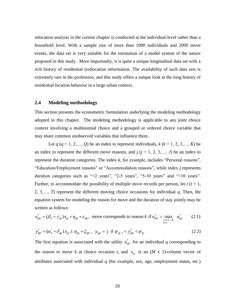
2.3 Focus of current chapter
This study constitutes a follow-up to Beige and Axhausen 2006 by jointly modeling the
reason for relocation and the duration of stay at a location preceding the relocation,
recognizing that the reason for location may itself be an endogenous variable influenced
24
by observed and unobserved variables. Much of the literature has treated the decision to
move as a binary choice decision (move/no-move) and modeled this decision as a
function of various factors, including the reason to move as an exogenous variable. Other
studies have used hazard-based duration models to represent the sojourn at a location
between moves, once again treating the reason for a move as an exogenous variable.
This study extends these previous studies in three important ways. First, the move
decision (whether or not to move and the reason for the move) is treated as an
endogenous variable in a multinomial unordered choice modeling framework as opposed
to being considered as an exogenous variable. Second, the duration of stay is modeled as
a grouped choice, with explicit accounting for the presence of unobserved variables that
may simultaneously impact duration of stay and primary reason for move. Modeling the
duration of stay as a grouped choice variable recognizes that individuals and households
treat the duration of stay at a residential location in terms of time-period ranges as
opposed to exact continuous durations. Third, we accommodate heterogeneity (or
variation in effect) of exogenous variables (i.e., random coefficients) in both the equation
for the move as well as the equation for the duration of stay preceding a re-location. To
our knowledge, this is the first application of such a joint unordered choice-grouped
choice model system with random coefficients.
The joint modeling of the move decision and the stay duration is important
because they are simultaneous decisions in the sense of being contemporaneous – An end
of stay duration occurs when a person decides to move out for a certain reason. In this
sense, one choice cannot structurally cause the other. Rather, the move decision and the
stay duration represent a package choice. Thus, the joint nature of the two decisions
arises because the choices are caused or determined by certain common underlying
observed and unobserved factors (see Train 1986, page 85). For example, high income
households may be more likely to move to upgrade their housing stock, and these same
households may also stay for shorter durations in any one residential location. Thus, there
is jointness among the choices because of a common underlying observed variable.
Similarly, a household‟s intrinsic (unobserved) preference for change (or quick satiation
25
with current housing attributes or neighborhood characteristics) may make the household
more likely to move to seek new housing attributes or a new neighborhood as well as
reduce stay durations at any single residential location. The association between the
reason to move and the stay duration in this case arises because of a common underlying
unobserved preference measure. Ignoring this error correlation due to unobserved factors,
and using the reason to move as an exogenous variable in a model of stay duration (or
estimating separate stay duration equations for each move reason), will, in general, result
in econometrically inconsistent estimates due to classic sample selection problems (see
Greene 2000, page 926 for a textbook treatment of this issue). Intuitively speaking, the
stay duration sample corresponding to the move reason of seeking new housing attributes
will be characterized by short stay durations (because of the common unobserved
intrinsic preference for change). If we use this “biased” sample for stay duration
modeling, the resulting stay duration estimates will not be appropriate for a randomly
picked household. But by modeling both reason for move and the stay duration, and
accounting for unobserved error correlation, the estimation effectively accounts for the
“bias” due to common unobserved preferences and is able to return unbiased stay
duration estimates that will be appropriate for a randomly picked household.
The model system takes the form of a joint unordered discrete choice – grouped
discrete choice model system with correlated error structures across the two choice
dimensions and random coefficients in each choice dimension. Specifically, the reason
for moving is modeled as a mixed multinomial logit (MNL). The duration of stay could
be modeled as a continuous variable; however, the data set used in this study and the
discrete nature of moving events lends itself more appropriately to the representation of
duration of stay as a grouped (ordered) choice variable in this particular study. The
mixed grouped logit model formulation is used to represent the duration of stay choice.
The data set used in this study is derived from a survey conducted in Zurich, Switzerland
that collected detailed information about residential relocations and the primary reason
for each relocation event for one individual (aged 18 years or older) in the household
over the 20 year period from 1985-2004 (as a result of this individual-level focus, the
26
relocation analysis in the current chapter is conducted at the individual-level rather than a
household level. With a sample size of more than 1000 individuals and 2000 move
events, the data set is very suitable for the estimation of a model system of the nature
proposed in this study. More importantly, it is quite a unique longitudinal data set with a
rich history of residential (re)location information. The availability of such data sets is
extremely rare in the profession, and this study offers a unique look at the long history of
residential location behavior in a large urban context.
2.4 Modeling methodology
This section presents the econometric formulation underlying the modeling methodology
adopted in this chapter. The modeling methodology is applicable to any joint choice
context involving a multinomial choice and a grouped or ordered choice variable that
may share common unobserved variables that influence them.
Let q (q = 1, 2,…, Q) be an index to represent individuals, k (k = 1, 2, 3,…, K) be
an index to represent the different move reasons, and j (j = 1, 2, 3,…, J) be an index to
represent the duration categories. The index k, for example, includes “Personal reasons”,
“Education/Employment reasons” or “Accommodation reasons”, while index j represents
duration categories such as “<2 years”, “2-5 years”, “5-10 years” and “>10 years”.
Further, to accommodate the possibility of multiple move records per person, let t (t = 1,
2, 3,…, T) represent the different moving choice occasions for individual q. Then, the
equation system for modeling the reason for move and the duration of stay jointly may be
written as follows:
* ' ' * *
1,2,...( ) , move corresponds to reason if max qkt k qk qt qk qkt qkt qit
i Kk i
u x k u u
(2.1)
* ' '( )qkt k qk qt qk qkty x , qkty j if *
1kj qtk kjy (2.2)
The first equation is associated with the utility *
qktu for an individual q corresponding to
the reason to move k at choice occasion t, and qtx is an (M x 1)-column vector of
attributes associated with individual q (for example, sex, age, employment status, etc.)
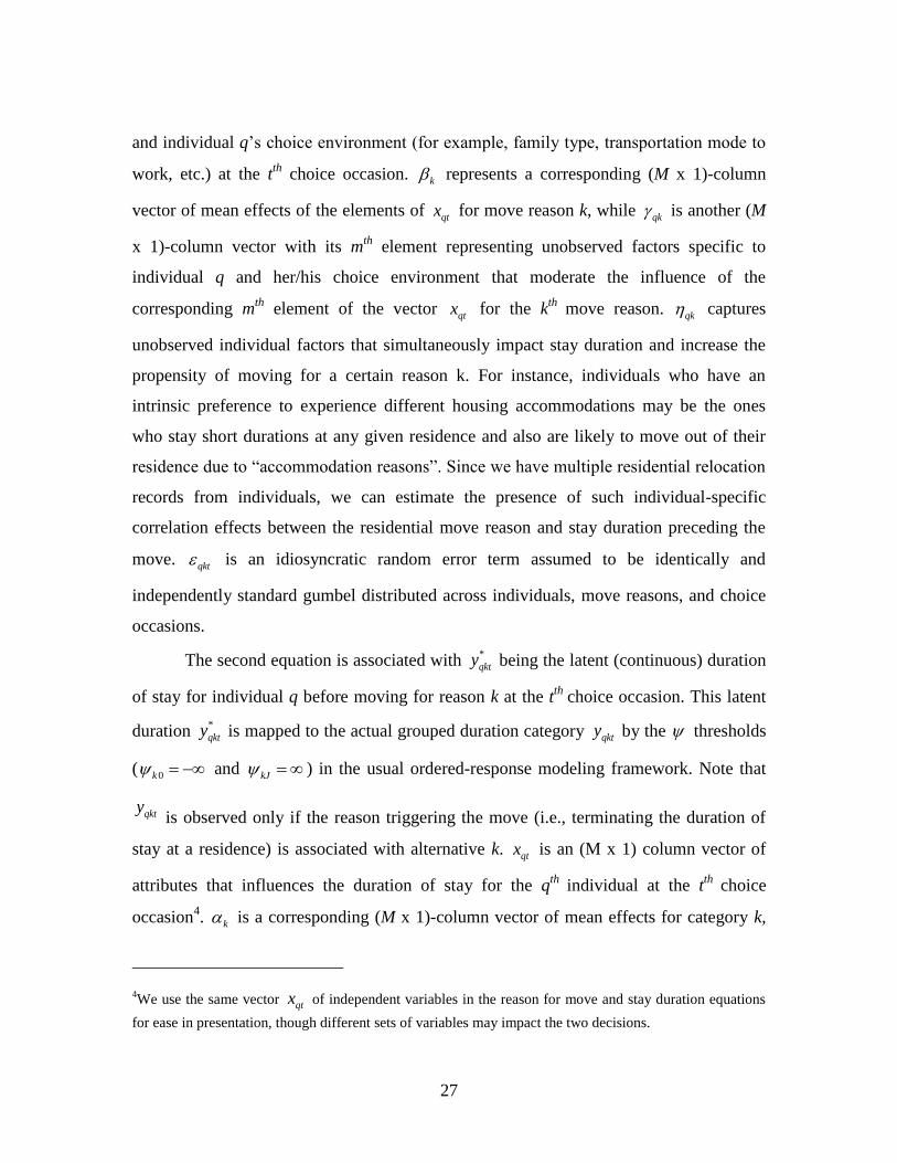
27
and individual q‟s choice environment (for example, family type, transportation mode to
work, etc.) at the tth
choice occasion. k represents a corresponding (M x 1)-column
vector of mean effects of the elements of qtx for move reason k, while
qk is another (M
x 1)-column vector with its mth
element representing unobserved factors specific to
individual q and her/his choice environment that moderate the influence of the
corresponding mth
element of the vector qtx for the k
th move reason.
qk captures
unobserved individual factors that simultaneously impact stay duration and increase the
propensity of moving for a certain reason k. For instance, individuals who have an
intrinsic preference to experience different housing accommodations may be the ones
who stay short durations at any given residence and also are likely to move out of their
residence due to “accommodation reasons”. Since we have multiple residential relocation
records from individuals, we can estimate the presence of such individual-specific
correlation effects between the residential move reason and stay duration preceding the
move. qkt is an idiosyncratic random error term assumed to be identically and
independently standard gumbel distributed across individuals, move reasons, and choice
occasions.
The second equation is associated with *
qkty being the latent (continuous) duration
of stay for individual q before moving for reason k at the tth
choice occasion. This latent
duration *
qkty is mapped to the actual grouped duration category qkty by the thresholds
( 0k and kJ ) in the usual ordered-response modeling framework. Note that
qkty is observed only if the reason triggering the move (i.e., terminating the duration of
stay at a residence) is associated with alternative k. qtx is an (M x 1) column vector of
attributes that influences the duration of stay for the qth
individual at the tth
choice
occasion4. k is a corresponding (M x 1)-column vector of mean effects for category k,
4We use the same vector qtx of independent variables in the reason for move and stay duration equations
for ease in presentation, though different sets of variables may impact the two decisions.
28
and qk is another (M x 1)-column vector of unobserved factors moderating the influence
of attributes in qtx on the duration of stay for individual q if the stay is terminated due to
reason k. qkt is an idiosyncratic random error term, assumed identically and
independently logistic distributed (across individuals, reasons for move, and choice
occasions) with variance 2 . In the current empirical context, the thresholds are
known (corresponding to the boundaries of the grouped categories), allowing us to
estimate the variance of qkt .
The sign in front of qk in the duration category equation indicates that the
correlation in unobserved individual factors between the reason to move and the duration
of stay may be positive or negative. A positive sign implies that unobserved factors that
increase the propensity of a move for a given reason will also increase the duration of
stay preceding such a potential move, while a negative sign suggests that unobserved
individual factors that increase the propensity of a move for a certain reason will decrease
the duration of stay preceding such a potential move. Clearly, one expects, from an
intuitive standpoint, that the latter case will hold, as also indicated in the initial discussion
of qk in the context of the first equation. However, one can empirically test the models
with both „+‟ and „−‟ signs to determine the best empirical result.
To complete the model structure of the system in Equations (2.1) and (2.2), it is
necessary to specify the structure for the unobserved vectors qk , qk , and qk . In this
chapter, it is assumed that the qk , qk , and qk elements are independent realizations
from normal population distributions; 2~ (0, )qkm kmN ,
2~ (0, )qkm kmN , and
2~ (0, )qk kN . With these assumptions, the probability expressions for the reason to
move and the duration category choices may be derived. Conditional on qk and qk for
each (and all) k, the probability of an individual q choosing to move for reason k at the tth
choice occasion is given by:
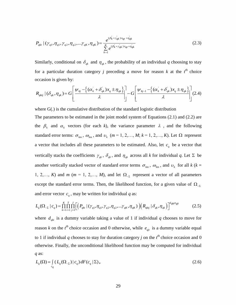
29
' ' '( )
1 1 2 2 ' ' '( )
1
| ( , , , ,... , )
xk qk qt qk
qkt q q q q qK qK K xk qk qt qk
k
eP
e
(2.3)
Similarly, conditional on qk and qk , the probability of an individual q choosing to stay
for a particular duration category j preceding a move for reason k at the tth
choice
occasion is given by:
' ' ' '
1( ) ( )| ( , )
kj k qk q qk kj k qk q qk
qktj qk qk
x xR G G
(2.4)
where G(.) is the cumulative distribution of the standard logistic distribution
The parameters to be estimated in the joint model system of Equations (2.1) and (2.2) are
the k and k vectors (for each k), the variance parameter , and the following
standard error terms: km ,
km , and k (m = 1, 2,…, M; k = 1, 2,…, K). Let represent
a vector that includes all these parameters to be estimated. Also, let qc be a vector that
vertically stacks the coefficients qk , qk , and qk across all k for individual q. Let be
another vertically stacked vector of standard error terms km , km , and k for all k (k =
1, 2,…, K) and m (m = 1, 2,…, M), and let represent a vector of all parameters
except the standard error terms. Then, the likelihood function, for a given value of
and error vector qc , may be written for individual q as:
1 1 2 21 1 1
( | ) | ( , , , ,... , ) | ,K T J d eqkt qjt
q q qkt q q q q qK qK qktj qk qkk t j
L c P R
(2.5)
where qktd is a dummy variable taking a value of 1 if individual q chooses to move for
reason k on the tth
choice occasion and 0 otherwise, while qjte is a dummy variable equal
to 1 if individual q chooses to stay for duration category j on the tth
choice occasion and 0
otherwise. Finally, the unconditional likelihood function may be computed for individual
q as:
( ) ( ( ) | ) ( | )q q q qcq
L L c dF c , (2.6)
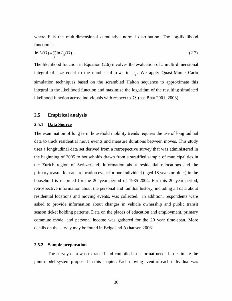
30
where F is the multidimensional cumulative normal distribution. The log-likelihood
function is
ln ( ) ln ( )qq
L L . (2.7)
The likelihood function in Equation (2.6) involves the evaluation of a multi-dimensional
integral of size equal to the number of rows in qc . We apply Quasi-Monte Carlo
simulation techniques based on the scrambled Halton sequence to approximate this
integral in the likelihood function and maximize the logarithm of the resulting simulated
likelihood function across individuals with respect to (see Bhat 2001, 2003).
2.5 Empirical analysis
2.5.1 Data Source
The examination of long term household mobility trends requires the use of longitudinal
data to track residential move events and measure durations between moves. This study
uses a longitudinal data set derived from a retrospective survey that was administered in
the beginning of 2005 to households drawn from a stratified sample of municipalities in
the Zurich region of Switzerland. Information about residential relocations and the
primary reason for each relocation event for one individual (aged 18 years or older) in the
household is recorded for the 20 year period of 1985-2004. For this 20 year period,
retrospective information about the personal and familial history, including all data about
residential locations and moving events, was collected. In addition, respondents were
asked to provide information about changes in vehicle ownership and public transit
season ticket holding patterns. Data on the places of education and employment, primary
commute mode, and personal income was gathered for the 20 year time-span. More
details on the survey may be found in Beige and Axhausen 2006.
2.5.2 Sample preparation
The survey data was extracted and compiled in a format needed to estimate the
joint model system proposed in this chapter. Each moving event of each individual was
31
associated with one of the following alternatives, with the final alternative being the “No
move” alternative:
Family reasons only (Fam)
Education/Employment reasons only (Edu)
Accommodation (size) related reasons only (Acc)
Surrounding environment related reasons and proximity to family and friends
only (SuVi)
Any two of the above reasons (Two)
All of the remaining types/reasons of moves (Oth)
No move in the 20 year period (NM)
The durations were coded into the following four ordered categories:
Less than 2 years
Two years or more, but less than 5 years
Five years or more, but less than 10 years
Greater than 10 years
The data set was compiled at the person level to reflect the fact that households
undergo transformations over a 20-year time period and that it makes more sense to track
individuals over time as opposed to whole households. Only those records that had
complete information for the entire 20 year period were included in the final data set for
analysis. The final data set includes 1012 individuals and 2590 move records. It is to be
noted that the move records do not include the first move that an individual reported in
the survey. As the move prior to 1985 is not known, there is no way to calculate the
duration of stay prior to the first move reported in the survey. Thus, each move record in
the database includes a primary reason for move and a duration category reflecting the
duration of stay prior to the reported move event.
32
A comprehensive descriptive analysis of the data set was undertaken prior to
model specification and estimation. A concise descriptive tabulation of key variables is
presented in Table 2.1.
2.5.3 Model structures estimated
In this study, three different model structures were estimated to facilitate comparisons
and to evaluate the efficacy of employing the correlated joint model system proposed in
this chapter. The three models are:
(1) A simple multinomial logit model for reason to move and an independent grouped
response model for duration of stay, referred to as the Independent Multinomial
Ordered (IMO) model
(2) A random coefficients multinomial logit model for reason to move and an
independent random coefficients grouped response model for duration of stay,
referred to as the Independent Random Multinomial Ordered (IRMO) model
(3) A random coefficients multinomial logit model for reason to move and a
correlated random coefficients grouped response model for duration of stay,
referred to as the Correlated Random Multinomial Ordered (CRMO) model.
In the context of the modeling methodology presented earlier in the chapter, the IMO
model imposes assumptions that km = 0, km = 0, and k = 0 for all k and m. The IRMO
model imposes the assumption that k = 0 for all k. The final specification of the random
coefficients in the reason to move and duration of stay components of the IRMO and
CRMO models were obtained after extensive testing. For the sake of brevity, only the
CRMO model estimation results are presented in detail in the chapter; however, the IMO
and IRMO models will be used as baseline model specifications to evaluate the efficacy
of using the CRMO model structure.

33
2.5.4 CRMO model estimation results
Three primary categories of variables were considered for inclusion in the models.
The first category includes individual characteristics such as age, gender, and
employment/education status of the person at the time of move. The second category
includes household characteristics such as household size, household type (family
structure and life cycle stage), household income, and vehicle ownership. Finally, the
third category includes commute characteristics including mode of transportation to work
and commute distance. Interaction effects among these categories of variables were also
considered and tested prior to arriving at the final model specification. The final model
specification was driven by intuitive judgment, parsimony in specification, and statistical
significance testing.
2.5.4.1 Residential move component
Model estimation results for the reason to move component of the CRMO model
are presented in Table 2.2. Consistent with the multinomial logit structure for this model
component, there are seven utility equations corresponding to each reason category. One
of the alternative specific constants is set to zero and there is at least one base category
for the introduction of other variables (in the Table all categories for a particular variable
with a „-‟ indication together form the base i.e. an effective coefficient of zero for
interpreting the effects of the variable). Consistent with the descriptive statistical analysis
presented in Table 2.1, all other things being equal, family and education/employment
reasons are more likely to trigger a move than other reasons as evidenced by the higher
alternative specific constants for these two reasons. Another major finding worthy of
being highlighted at the outset is that there were no statistically significant unobserved
effects in the “reason to move” model.
Among individual characteristics, it is found that females are more likely to move
due to family-related or personal reasons. Those in the age bracket of 31-45 years are
less likely to move for family-related or education/employment reasons; these effects are
more pronounced for those over the age of 45 years. In general, it appears that
34
individuals who have reached a lifecycle stage where they have settled into a household
and/or family setting are less likely to move for these specific reasons. Usually families
are quite stable in these age ranges; family transitions occur either when individuals are
young due to such events as marriage, gaining employment, or birth of a child, or when
they are old due to such events as retirement, children growing up and leaving home,
death of a spouse, or physical limitations set in. Those who are employed are more likely
to move for reasons related to the nature of the accommodation (e.g., desiring to move to
a larger home), for multiple reasons (which may include family and
education/employment related factors), or for other reasons. Thus, it appears that
employed individuals tend to be more inclined to move in comparison to unemployed
individuals.
Among household characteristics, it is found that larger households are more
likely to not move as evidenced by the positive coefficient associated with household size
in the no-move equation. It is likely that larger households are mature, with children, and
have stable situations that have them inclined to stay in place for longer durations. In
comparison to single-person households, family households are less likely to move for
education/employment or surrounding/vicinity related reasons. Again, these households
are likely to be in more stable situations in the life cycle and hence more disinclined to
move for these reasons. Individuals in non-family households, on the other hand, are
more prone to move as evidenced by the negative coefficient associated with this variable
in the no-move equation. Individuals in non-family households are less likely to have
family-related roots in their current situation, and would therefore be more likely to move
as they transition to more stable stages of their lifecycle. The notion of stability and its
influence in reducing the likelihood of moving for various reasons is further confirmed
by the negative coefficient associated with the home ownership variable. Those living in
households who own their home are less likely to move for family,
education/employment, and surrounding vicinity-related reasons. In other words, when
such households do move, it is likely to be due to accommodation-related reasons or
combinations of factors.
35
Commute characteristics are also found to play an important role in influencing
individual residential mobility for various reasons. In comparison to those who commute
by car, those who use alternate modes of transportation are more likely to move for
various reasons, a finding that is rather noteworthy in the context of transport policy
debates. Those who commute by bicycle appear to be most prone to moving for a variety
of reasons such as education/employment, accommodation, surrounding vicinity, and a
multitude of factors. Those who use public transit are more likely to move for
education/employment reasons, surrounding vicinity, and other reasons. In both of these
instances, it is possible that the individuals who use these modes of transportation are in
neighborhoods or employment situations that are transient or less desirable. Further,
those who walk are likely to move for education/employment reasons, but less likely to
move for accommodation or surrounding vicinity related reasons. It appears that those
who live within a comfortable walking distance from work are pleased with their
neighborhood; hence, any move is triggered by an education/employment related reason
as opposed to a neighborhood or housing related reason. Finally, if one commutes more
than 10 km to work, then the likelihood of not moving reduces; in other words those who
commute longer distances are likely to move, presumably to find a more palatable
commuting distance.
2.5.4.2 Stay duration component
The stay duration component of the model system is presented in Table 2.3. It is
to be noted that there are six possible duration equations that can be estimated, one for
each reason to move. After extensive testing and model estimation runs, it was found that
there were no significant differences across model coefficients among the different
reasons; therefore, virtually all parameters (except for a couple of constants) are identical
across the six move reasons.
Among individual characteristics, females are likely to have shorter stay durations
across all reasons for moving. It is not immediately clear as to why this is the case and
further exploration of the basis for this finding is warranted in future research on this
36
topic. Age exhibits a non-linear effect with the square of age showing a negative effect,
but the square of age showing a positive effect. This parabolic relationship means that, as
age increases, the duration of stay tends to decrease. However, this tendency peaks at the
age of 39 years and reduces with age until individuals are about 75 years old. After the
age of 75 years, there is an overall positive impact of age on duration of stay. Thus, it
appears that people move when they are young, but the frequency of moving decreases
(thus, durations get longer) after the age of 39 until the age of 75 years. After the age of
75, individuals tend to be quite stable in place, contributing to the positive effect on the
square of age.
Among household characteristics, individuals in larger households tend to have
longer stay durations, consistent with earlier findings that these individuals are less likely
to move. However, it is noteworthy that the impact of household size exhibits variability
across the population as indicated by the statistically significant standard deviation on the
unobserved component associated with household size variable. Thus, this model
specification captures unobserved heterogeneity in the population with respect to
household size effects. An individual in a non-family household tends have shorter stay
durations, while an individual in a household that owns its home tends to have longer stay
durations. Individuals in smaller houses (with just one or two rooms) tend to have shorter
stay durations as evidenced by the negative coefficient associated with this variable.
Presumably, these individuals are more prone to moving frequently as they attempt to
upgrade to larger and more spacious homes. Finally, those commuting by public
transportation and bicycle tend to have shorter stay durations, consistent with the findings
reported in the reason-to-move model. Also, those commuting more than 10 km tend to
have shorter stay durations as well, presumably because they move more frequently in
search of housing that reduces their commute.
The CRMO model presented in Tables 2.2 and 2.3 clearly shows the importance
of capturing the correlation across the move reason and the duration of stay phenomena
(see the last row of Table 2.3, which presents the k estimates). In the estimations, we
considered both the positive and negative signs on the qk terms in Equation (2.2) for
37
each (and all) k, and the negative sign for all k provided statistically superior results.
Also, the standard error (deviation) estimates were not statistically different in magnitude
across the move regimes, and so were constrained to be equal across regimes. The
magnitude and significance of the standard deviations of the qk terms, along with the
negative sign on these terms in Equation (2.2), confirms our hypothesis of the presence of
a negative correlation due to common unobserved individual elements between the
propensity to move and the corresponding duration of stay for each move regime k.
2.5.5 Model assessment
As mentioned earlier, three distinct model systems were estimated. The IMO and IRMO
model systems offered nearly identical statistical goodness-of-fit measures. The log-
likelihood value at convergence for the IMO model is -7397.9 with 44 parameters, while
that for the IRMO model is -7397.1 with 45 parameters. A likelihood ratio test
comparison between these models does not reject the hypotheses that these two models
are identical with respect to statistical fit. On the other hand, the CRMO model yields a
log-likelihood value of -7227.2 with 46 parameters. Likelihood ratio test statistics show
that the CRMO offers significantly better goodness-of-fit at any level of significance.
This finding further corroborates that accounting for error correlation across the reason-
to-move and stay-duration equations results in statistically superior parameter estimates.
2.6 Summary
The current chapter focuses on modeling household residential relocation decisions. In
particular, the emphasis is on jointly modeling the reason for residential relocation and
the associated duration of stay. The chapter formulates an econometric framework to
model these choices in a unified framework. The model in this chapter takes the form of a
joint multinomial logit model of reason for move and a grouped logit model of residential
stay duration preceding the move. The econometric model formulated is applied for
actual data using data drawn from a 2005 retrospective survey in the Zurich region of
Switzerland. Several demographic, socio-economic, and commute related variables are
38
found to significantly influence the reason for move and the duration of stay. What is
most important in the context of this study is the finding that there are common
unobserved factors affecting the reason to move and the duration of stay choices. This
simultaneity or endogeneity between the choice processes clearly calls for modeling these
two choice dimensions in a joint modeling framework that accommodates error
correlation structures. In addition, in the duration of stay model, it was found that the
impact of household size exhibited heterogeneity across the sample of individuals
considered in this study. Goodness-of-fit measures were significantly superior for the
joint correlated model structure, clearly favoring the use of the model framework
presented here for modeling residential mobility processes.
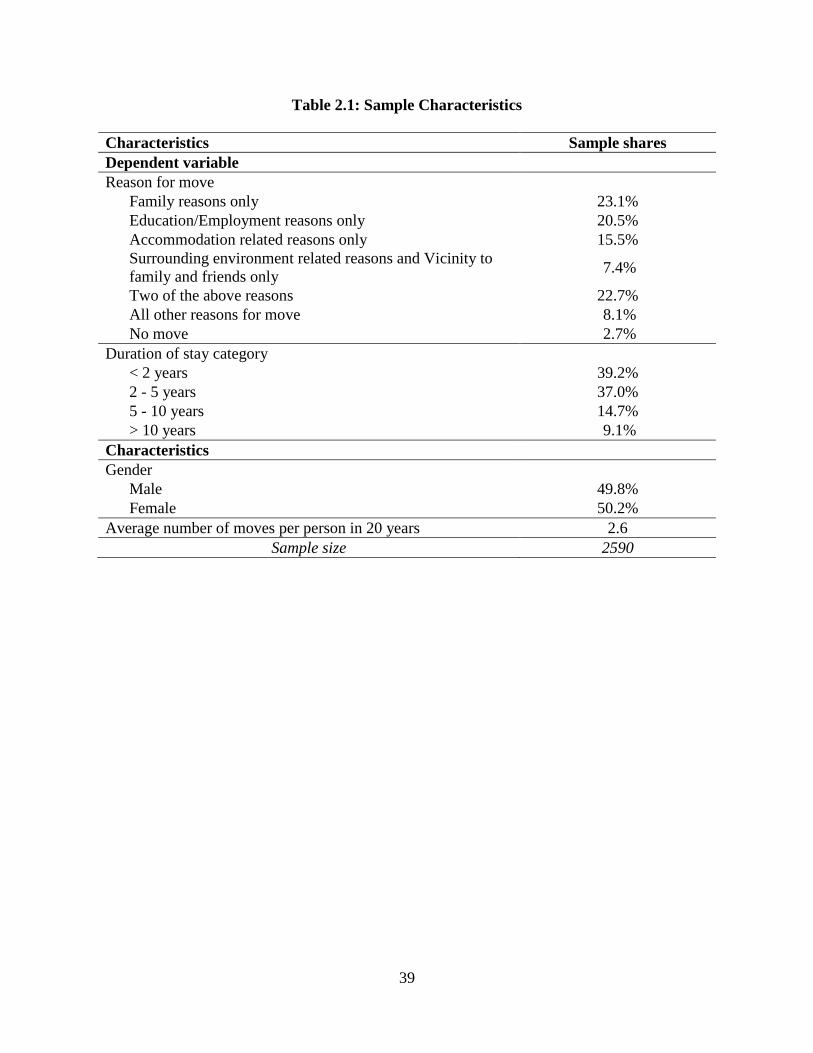
39
Table 2.1: Sample Characteristics
Characteristics Sample shares
Dependent variable
Reason for move
Family reasons only 23.1%
Education/Employment reasons only 20.5%
Accommodation related reasons only 15.5%
Surrounding environment related reasons and Vicinity to
family and friends only 7.4%
Two of the above reasons 22.7%
All other reasons for move 8.1%
No move 2.7%
Duration of stay category
< 2 years 39.2%
2 - 5 years 37.0%
5 - 10 years 14.7%
> 10 years 9.1%
Characteristics
Gender
Male 49.8%
Female 50.2%
Average number of moves per person in 20 years 2.6
Sample size 2590
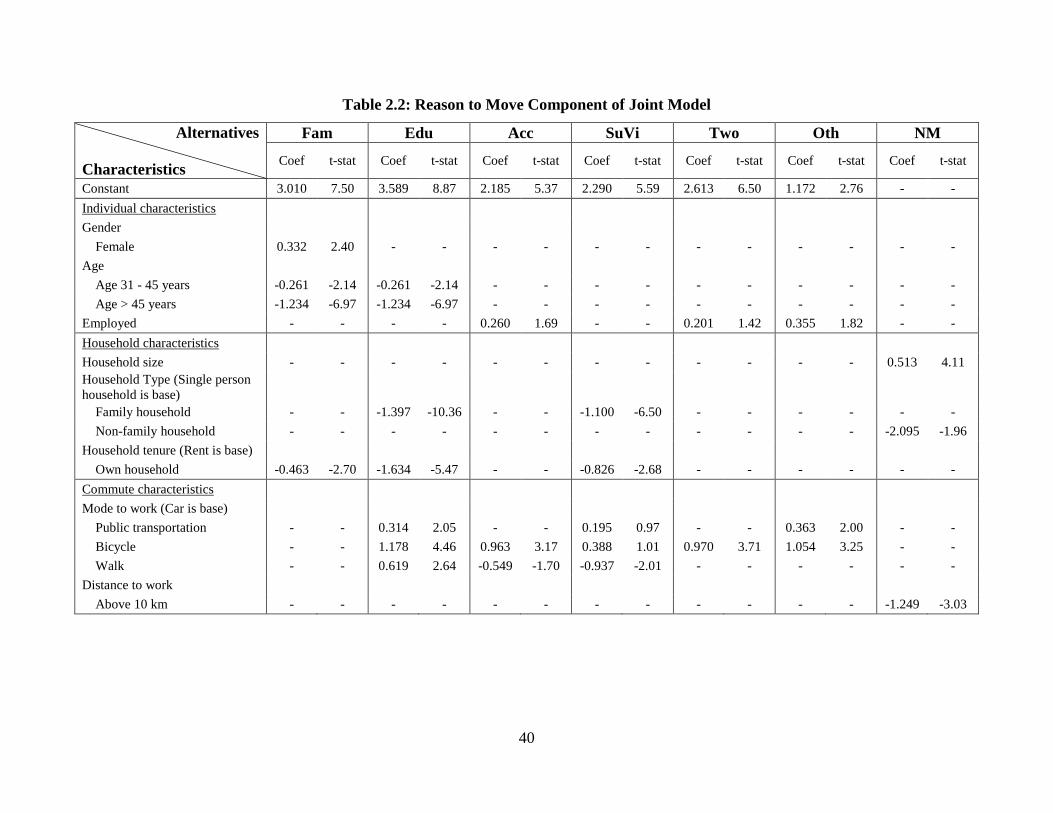
40
Table 2.2: Reason to Move Component of Joint Model
Alternatives
Characteristics
Fam Edu Acc SuVi Two Oth NM
Coef t-stat Coef t-stat Coef t-stat Coef t-stat Coef t-stat Coef t-stat Coef t-stat
Constant 3.010 7.50 3.589 8.87 2.185 5.37 2.290 5.59 2.613 6.50 1.172 2.76 - -
Individual characteristics
Gender
Female 0.332 2.40 - - - - - - - - - - - -
Age
Age 31 - 45 years -0.261 -2.14 -0.261 -2.14 - - - - - - - - - -
Age > 45 years -1.234 -6.97 -1.234 -6.97 - - - - - - - - - -
Employed - - - - 0.260 1.69 - - 0.201 1.42 0.355 1.82 - -
Household characteristics
Household size - - - - - - - - - - - - 0.513 4.11
Household Type (Single person
household is base)
Family household - - -1.397 -10.36 - - -1.100 -6.50 - - - - - -
Non-family household - - - - - - - - - - - - -2.095 -1.96
Household tenure (Rent is base)
Own household -0.463 -2.70 -1.634 -5.47 - - -0.826 -2.68 - - - - - -
Commute characteristics
Mode to work (Car is base)
Public transportation - - 0.314 2.05 - - 0.195 0.97 - - 0.363 2.00 - -
Bicycle - - 1.178 4.46 0.963 3.17 0.388 1.01 0.970 3.71 1.054 3.25 - -
Walk - - 0.619 2.64 -0.549 -1.70 -0.937 -2.01 - - - - - -
Distance to work
Above 10 km - - - - - - - - - - - - -1.249 -3.03
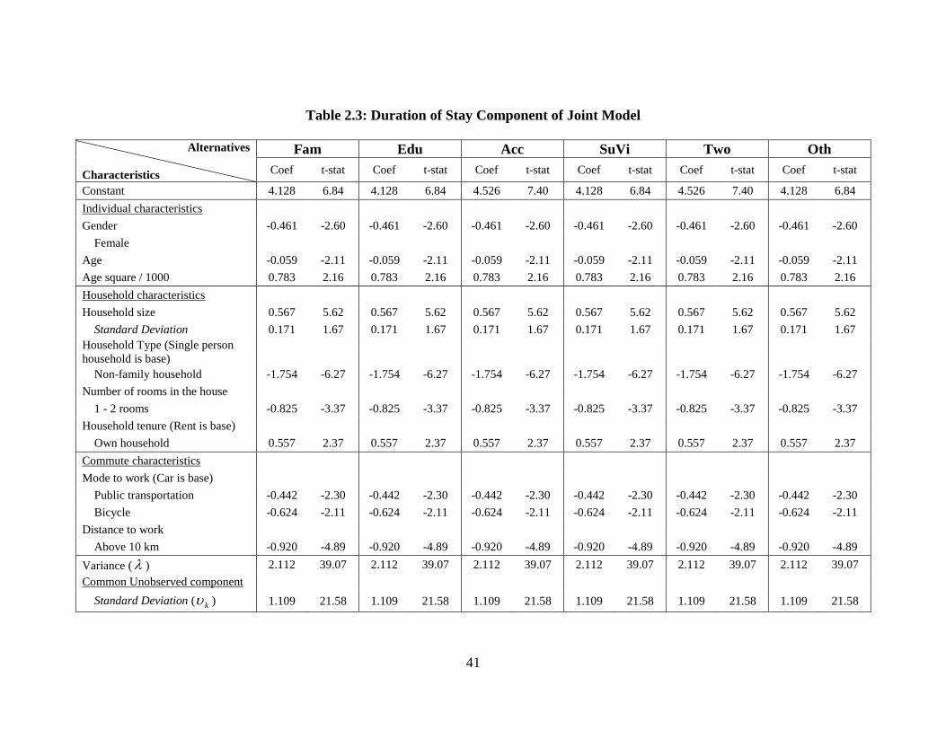
41
Table 2.3: Duration of Stay Component of Joint Model
Alternatives
Characteristics
Fam Edu Acc SuVi Two Oth
Coef t-stat Coef t-stat Coef t-stat Coef t-stat Coef t-stat Coef t-stat
Constant 4.128 6.84 4.128 6.84 4.526 7.40 4.128 6.84 4.526 7.40 4.128 6.84
Individual characteristics
Gender -0.461 -2.60 -0.461 -2.60 -0.461 -2.60 -0.461 -2.60 -0.461 -2.60 -0.461 -2.60
Female
Age -0.059 -2.11 -0.059 -2.11 -0.059 -2.11 -0.059 -2.11 -0.059 -2.11 -0.059 -2.11
Age square / 1000 0.783 2.16 0.783 2.16 0.783 2.16 0.783 2.16 0.783 2.16 0.783 2.16
Household characteristics
Household size 0.567 5.62 0.567 5.62 0.567 5.62 0.567 5.62 0.567 5.62 0.567 5.62
Standard Deviation 0.171 1.67 0.171 1.67 0.171 1.67 0.171 1.67 0.171 1.67 0.171 1.67
Household Type (Single person
household is base)
Non-family household -1.754 -6.27 -1.754 -6.27 -1.754 -6.27 -1.754 -6.27 -1.754 -6.27 -1.754 -6.27
Number of rooms in the house
1 - 2 rooms -0.825 -3.37 -0.825 -3.37 -0.825 -3.37 -0.825 -3.37 -0.825 -3.37 -0.825 -3.37
Household tenure (Rent is base)
Own household 0.557 2.37 0.557 2.37 0.557 2.37 0.557 2.37 0.557 2.37 0.557 2.37
Commute characteristics
Mode to work (Car is base)
Public transportation -0.442 -2.30 -0.442 -2.30 -0.442 -2.30 -0.442 -2.30 -0.442 -2.30 -0.442 -2.30
Bicycle -0.624 -2.11 -0.624 -2.11 -0.624 -2.11 -0.624 -2.11 -0.624 -2.11 -0.624 -2.11
Distance to work
Above 10 km -0.920 -4.89 -0.920 -4.89 -0.920 -4.89 -0.920 -4.89 -0.920 -4.89 -0.920 -4.89
Variance ( ) 2.112 39.07 2.112 39.07 2.112 39.07 2.112 39.07 2.112 39.07 2.112 39.07
Common Unobserved component
Standard Deviation ( k ) 1.109 21.58 1.109 21.58 1.109 21.58 1.109 21.58 1.109 21.58 1.109 21.58
42
CHAPTER 3 EXAMINING THE INFLUENCE OF BUILT
ENVIRONMENT ON TRAVEL DEMAND
3.1 Introduction
There has been considerable interest in the land use-transportation connection in the past
decade, motivated by the possibility that land-use and urban form design policies can be
used to control, manage, and shape individual traveler behavior and aggregate travel
demand. A central issue in this regard is the debate whether any effect of the built
environment on travel demand is causal or merely associative (or some combination of
the two; see Bhat and Guo, 2007). To explicate this, consider a cross-sectional sample of
households, some of whom live in a neo-urbanist neighborhood and others of whom live
in a conventional neighborhood. A neo-urbanist neighborhood is one with high
population density, high bicycle lane and roadway street density, good land-use mix, and
good transit and non-motorized mode accessibility/facilities. A conventional
neighborhood is one with relatively low population density, low bicycle lane and
roadway street density, primarily single use residential land use, and auto-dependent
urban design. Assume that the vehicle miles of travel (VMT) of households living in
conventional neighborhoods is higher than the VMT of households residing in neo-
urbanist neighborhoods. The question is whether this difference in VMT between
households in conventional and neo-urbanist households is due to “true” effects of the
built environment, or due to households self-selecting themselves into neighborhoods
based on their VMT desires. For instance, it is at least possible (if not likely) that
unobserved factors that increase the propensity or desire of a household to reside in a
conventional neighborhood (such as overall auto inclination, a predisposition to enjoying
travel, safety and security concerns regarding non-auto travel, etc.) also lead to the
household putting more vehicle miles of travel on personal vehicles. If this self selection
is not accounted for, the difference in VMT attributed directly to the variation in the built
environment between conventional and neo-urbanist neighborhoods can be mis-
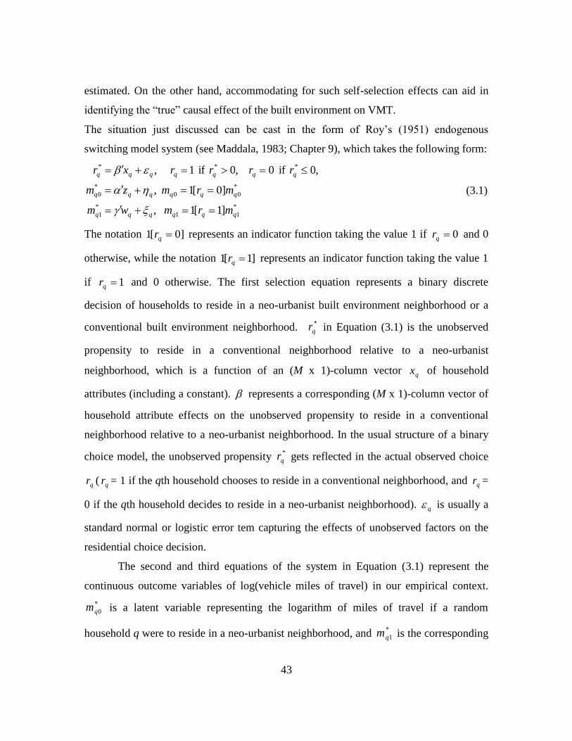
43
estimated. On the other hand, accommodating for such self-selection effects can aid in
identifying the “true” causal effect of the built environment on VMT.
The situation just discussed can be cast in the form of Roy‟s (1951) endogenous
switching model system (see Maddala, 1983; Chapter 9), which takes the following form:
*
11
*
1
*
00
*
0
***
]1[1 ,
]0[1 ,
,0 if 0 ,0 if 1 ,
qqqqqq
qqqqqq
qqqqqqq
mrmwm
mrmzm
rrrrxr
(3.1)
The notation ]0[1 qr represents an indicator function taking the value 1 if 0qr and 0
otherwise, while the notation ]1[1 qr represents an indicator function taking the value 1
if 1qr and 0 otherwise. The first selection equation represents a binary discrete
decision of households to reside in a neo-urbanist built environment neighborhood or a
conventional built environment neighborhood. *
qr in Equation (3.1) is the unobserved
propensity to reside in a conventional neighborhood relative to a neo-urbanist
neighborhood, which is a function of an (M x 1)-column vector qx of household
attributes (including a constant). represents a corresponding (M x 1)-column vector of
household attribute effects on the unobserved propensity to reside in a conventional
neighborhood relative to a neo-urbanist neighborhood. In the usual structure of a binary
choice model, the unobserved propensity *
qr gets reflected in the actual observed choice
qr ( qr = 1 if the qth household chooses to reside in a conventional neighborhood, and qr =
0 if the qth household decides to reside in a neo-urbanist neighborhood). q is usually a
standard normal or logistic error tem capturing the effects of unobserved factors on the
residential choice decision.
The second and third equations of the system in Equation (3.1) represent the
continuous outcome variables of log(vehicle miles of travel) in our empirical context.
*
0qm is a latent variable representing the logarithm of miles of travel if a random
household q were to reside in a neo-urbanist neighborhood, and *
1qm is the corresponding
44
variable if the household q were to reside in a conventional neighborhood. These are
related to vectors of household attributes qz and qw , respectively, in the usual linear
regression fashion, with q and q being random error terms. Of course, we observe *
0qm
in the form of 0qm only if household q in the sample is observed to live in a neo-urbanist
neighborhood. Similarly, we observe *
1qm in the form of 1qm only if household q in the
sample is observed to live in a conventional neighborhood.
The potential dependence between the error pairs ),( qq and ),( qq has to be
expressly recognized in the above system, as discussed earlier from an intuitive
standpoint.5 The classic econometric estimation approach proceeds by using Heckman‟s
or Lee‟s approaches or their variants (Heckman, 1974, 1976, 1979, 2001, Greene, 1981,
Lee, 1982, 1983, Dubin and McFadden, 1984). Heckman‟s (1974) original approach used
a full information maximum likelihood method with bivariate normal distribution
assumptions for ),( qq and ),( qq . Lee (1983) generalized Heckman‟s approach by
allowing the univariate error terms ,, qq and q to be non-normal, using a technique to
transform non-normal variables into normal variates, and then adopting a bivariate
normal distribution to couple the transformed normal variables. Thus, while maintaining
an efficient full-information likelihood approach, Lee‟s method relaxes the normality
assumption on the marginals but still imposes a bivariate normal coupling. In addition to
these full-information likelihood methods, there are also two-step and more robust
parametric approaches that impose a specific form of linearity between the error term in
the discrete choice and the continuous outcome (rather than a pre-specified bivariate joint
distribution). These approaches are based on the Heckman method for the binary choice
case, which was generalized by Hay (1980) and Dubin and McFadden (1984) for the
multinomial case. The approach involves the first step estimation of the discrete choice
equation given distributional assumptions on the choice model error terms, followed by
5 The reader will note that it is not possible to identify any dependence parameters between (ηq, ξq) because
the vehicle miles of travel is observed in only one of the two regimes for any given household.
45
the second step estimation of the continuous equation after the introduction of a
correction term that is an estimate of the expected value of the continuous equation error
term given the discrete choice. However, these two-step methods do not perform well
when there is a high degree of collinearity between the explanatory variables in the
choice equation and the continuous outcome equation, as is usually the case in empirical
applications. This is because the correction term in the second step involves a non-linear
function of the discrete choice explanatory variables. But this non-linear function is
effectively a linear function for a substantial range, causing identification problems when
the set of discrete choice explanatory variables and continuous outcome explanatory
variables are about the same. The net result is that the two-step approach can lead to
unreliable estimates for the outcome equation (see Leung and Yu, 2000 and Puhani,
2000).
Overall, Lee‟s full information maximum likelihood approach has seen more
application in the literature relative to the other approaches just described because of its
simple structure, ease of estimation using a maximum likelihood approach, and its lower
vulnerability to the collinearity problem of two-step methods. But Lee‟s approach is also
critically predicated on the bivariate normality assumption on the transformed normal
variates in the discrete and continuous equation, which imposes the restriction that the
dependence between the transformed discrete and continuous choice error terms is linear
and symmetric. There are two ways that one can relax this joint bivariate normal coupling
used in Lee‟s approach. One is to use semi-parametric or non-parametric approaches to
characterize the relationship between the discrete and continuous error terms, and the
second is to test alternative copula-based bivariate distributional assumptions to couple
error terms. Each of these approaches is discussed in turn next.
3.1.1 Semi-Parametric and Non-Parametric Approaches
The potential econometric estimation problems associated with Lee‟s parametric
distribution approach has spawned a whole set of semi-parametric and non-parametric
two-step estimation methods to handle sample selection, apparently having beginnings in
46
the semi-parametric work of Heckman and Robb (1985). The general approach in these
methods is to first estimate the discrete choice model in a semi-parametric or non-
parametric fashion using methods developed by, among others, Cosslett (1983), Ichimura
(1993), Matzkin (1992, 1993), and Briesch et al. (2002). These estimates then form the
basis to develop an index function to generate a correction term in the continuous
equation that is an estimate of the expected value of the continuous equation error term
given the discrete choice. While in the two-step parametric methods, the index function is
defined based on the assumed marginal and joint distributional assumptions, or on an
assumed marginal distribution for the discrete choice along with a specific linear form of
relationship between the discrete and continuous equation error terms, in the semi- and
non-parametric approaches, the index function is approximated by a flexible function of
parameters such as the polynomial, Hermitian, or Fourier series expansion methods (see
Vella, 1998 and Bourguignon et al., 2007 for good reviews). But, of course, there are “no
free lunches”. The semi-parametric and non-parametric approaches involve a large
number of parameters to estimate, are relatively very inefficient from an econometric
estimation standpoint, typically do not allow the testing and inclusion of a rich set of
explanatory variables with the usual range of sample sizes available in empirical
contexts, and are difficult to implement. Further, the computation of the covariance
matrix of parameters for inference is anything but simple in the semi- and non-parametric
approaches. The net result is that the semi- and non-parametric approaches have been
pretty much confined to the academic realm and have seen little use in actual empirical
application.
3.1.2 The Copula Approach
The turn toward semi-parametric and non-parametric approaches to dealing with sample
selection was ostensibly because of a sense that replacing Lee‟s parametric bivariate
normal coupling with alternative bivariate couplings would lead to substantial
computational burden. However, an approach referred to as the “Copula” approach has
recently revived interest in maintaining a Lee-like sample selection framework, while
47
generalizing Lee‟s framework to adopt and test a whole set of alternative bivariate
couplings that can allow non-linear and asymmetric dependencies. A copula is essentially
a multivariate functional form for the joint distribution of random variables derived
purely from pre-specified parametric marginal distributions of each random variable. The
reasons for the interest in the copula approach for sample selection models are several.
First, the copula approach does not entail any more computational burden than Lee‟s
approach. Second, the approach allows the analyst to stay within the familiar maximum
likelihood framework for estimation and inference, and does not entail any kind of
numerical integration or simulation machinery. Third, the approach allows the marginal
distributions in the discrete and continuous equations to take on any parametric
distribution, just as in Lee‟s method. Finally, under the copula approach, Lee‟s coupling
method is but one of a suite of different types of couplings that can be tested.
In this chapter, we apply the copula approach to examine built environment
effects on vehicle miles of travel (VMT). The rest of this chapter is structured as follows.
The next section provides a theoretical overview of the copula approach, and presents
several important copula structures. Section 3.3 discusses the use of copulas in sample
selection models. Section 3.4 provides an overview of the data sources and sample used
for the empirical application. Section 3.5 presents and discusses the modeling results. The
final section concludes the chapter by highlighting its findings.
3.2 Overview of the copula approach
3.2.1 Background
The incorporation of dependency effects in econometric models can be greatly facilitated
by using a copula approach for modeling joint distributions, so that the resulting model
can be in closed-form and can be estimated using direct maximum likelihood techniques
(the reader is referred to Trivedi and Zimmer, 2007 or Nelsen, 2006 for extensive reviews
of copula theory, approaches, and benefits). The word copula itself was coined by Sklar,
1959 and is derived from the Latin word “copulare”, which means to tie, bond, or connect
(see Schmidt, 2007). Thus, a copula is a device or function that generates a stochastic
48
dependence relationship (i.e., a multivariate distribution) among random variables with
pre-specified marginal distributions. In essence, the copula approach separates the
marginal distributions from the dependence structure, so that the dependence structure is
entirely unaffected by the marginal distributions assumed. This provides substantial
flexibility in correlating random variables, which may not even have the same marginal
distributions.
The effectiveness of a copula approach has been recognized in the statistics field
for several decades now (see Schweizer and Sklar, 1983, Ch. 6), but it is only recently
that copula-based methods have been explicitly recognized and employed in the finance,
actuarial science, hydrological modeling, and econometrics fields (see, for example,
Embrechts et al., 2002, Cherubini et al., 2004, Frees and Wang, 2005, Genest and Favre,
2007, Grimaldi and Serinaldi, 2006, Smith, 2005, Prieger, 2002, Zimmer and Trivedi,
2006, Cameron et al., 2004, Junker and May, 2005, and Quinn, 2007). The precise
definition of a copula is that it is a multivariate distribution function defined over the unit
cube linking uniformly distributed marginals. Let C be a K-dimensional copula of
uniformly distributed random variables U1, U2, U3, …, UK with support contained in
[0,1]K. Then,
Cθ (u1, u2, …, uK) = Pr(U1 < u1, U2 < u2, …, UK < uK), (3.2)
where is a parameter vector of the copula commonly referred to as the dependence
parameter vector. A copula, once developed, allows the generation of joint multivariate
distribution functions with given marginals. Consider K random variables Y1, Y2, Y3, …,
YK, each with univariate continuous marginal distribution functions Fk(yk) = Pr(Yk < yk), k
=1, 2, 3, …, K. Then, by the integral transform result, and using the notation (.)1
kF for
the inverse univariate cumulative distribution function, we can write the following
expression for each k (k = 1, 2, 3, …, K):
)).(Pr())(Pr()Pr()( 1
kkkkkkkkkk yFUyUFyYyF (3.3)
Then, by Sklar‟s (1973) theorem, a joint K-dimensional distribution function of
the random variables with the continuous marginal distribution functions Fk(yk) can be
generated as follows:
49
F(y1, y2, …, yK) = Pr(Y1 < y1, Y2 < y2, …, YK < yK) = Pr(U1 < F1(y1),, U2 < F2(y2), …,UK <
FK(yK))
= Cθ (u1 = F1(y1), u2 = F2(y2),…, uK = FK(yK)). (3.4)
Conversely, by Sklar‟s theorem, for any multivariate distribution function with
continuous marginal distribution functions, a unique copula can be defined that satisfies
the condition in Equation (3.4).
Copulas themselves can be generated in several different ways, including the
method of inversion, geometric methods, and algebraic methods (see Nelsen, 2006; Ch.
3). For instance, given a known multivariate distribution F(y1, y2, …, yK) with continuous
margins Fk(yk), the inversion method inverts the relationship in Equation (3.4) to obtain a
copula:
Cθ (u1, u2, …, uK) = Pr(U1 < u1, U2 < u2, …, UK < uK)
= Pr(Y1 < F–1
1(u1), Y2 < F–1
2(u2), ..., Y3 < F–1
3(u3)) (3.5)
= F(y1 = F–1
1(u1), y2 = F–1
2(u2), ..., yK = F–1
k(uk)).
Once the copula is developed, one can revert to Equation (3.4) to develop new
multivariate distributions with arbitrary univariate margins.
A rich set of copula types have been generated using the inversion and other
methods, including the Gaussian copula, the Farlie-Gumbel-Morgenstern (FGM) copula,
and the Archimedean class of copulas (including the Clayton, Gumbel, Frank, and Joe
copulas). These copulas are discussed later in the context of bivariate distributions. In
such bivariate distributions, while θ can be a vector of parameters, it is customary to use a
scalar measure of dependence. In the next section, we discuss some copula properties and
dependence structure concepts for bivariate copulas, though generalizations to higher
dimensions are possible.
3.2.2 Copula Properties and Dependence Structure
Consider any bivariate copula ) ,( 21 uuC . Since this is a bivariate cumulative distribution
function, the copula should satisfy the well known Fréchet-Hoeffding bounds (see
50
Kwerel, 1988). Specifically, the Fréchet lower bound ) ,( 21 uuW is )0 ,1max( 21 uu and
the Fréchet upper bound ) ,( 21 uuM is ) ,min( 21 uu . Thus,
). ,() ,() ,( 212121 uuMuuCuuW (3.6)
From Sklar‟s theorem of Equation (3.4), we can also re-write the equation above
in terms of Fréchet bounds for the multivariate distribution ) ,( 21 yyF generated from the
copula ) ,( 21 uuC :
)).( ),(min() ,()0 ,1)()(max( 2211212211 yFyFyyFyFyF (3.7)
If the copula ) ,( 21 uuC is equal to the lower bound ) ,( 21 uuW in Equation (3.6),
or equivalently if ) ,( 21 yyF is equal to the lower bound in Equation (3.7), then the
random variables 1Y and 2Y are almost surely decreasing functions of each other and are
called “countermonotonic”. On the other hand, if the copula ) ,( 21 uuC is equal to the
upper bound ) ,( 21 uuM in Equation (3.6), or equivalently if ) ,( 21 yyF is equal to the
upper bound in Equation (3.7), then the random variables 1Y and 2Y are almost surely
increasing functions of each other and are called “comonotonic”. The case when
2121 ) ,( uuuuC , or equivalently )()() ,( 221121 yFyFyyF , corresponds to
stochastic independence between 1Y and 2Y .
Different copulas provide different levels of ability to capture dependence
between Y1 and Y2 based on the degree to which they cover the interval between the
Fréchet-Hoeffding bounds. Comprehensive copulas are those that (1) attain or approach
the lower bound W as θ approaches the lower bound of its permissible range, (2) attain or
approach the upper bound M as θ approaches its upper bound, and (3) cover the entire
domain between W and M (including the product copula case Π as a special or limiting
case). Thus, comprehensive copulas parameterize the full range of dependence as
opposed to non-comprehensive copulas that are only able to capture dependence in a
limited manner. As we discuss later, the Gaussian and Frank copulas are comprehensive
in their dependence structure, while the FGM, Clayton, Gumbel, and Joe copulas are not
comprehensive.
51
To better understand the generated dependence structures between the random
variables ) ,( 21 YY based on different copulas, and examine the coverage offered by non-
comprehensive copulas, it is useful to construct a scalar dependence measure between 1Y
and 2Y that satisfies four properties as listed below (see Embrechts et al., 2002):
(1) ),(),( 1221 YYYY
(2) 1),(1 21 YY (3.8)
(3) otoniccountermon ),(1 ),( c;comonotoni ),(1),( 21212121 YYYYYYYY
(4) )),(),((),( 221121 YGYGYY where 1G and 2G are two (possibly different)
strictly increasing transformations.
The traditional dependence concept of correlation coefficient (i.e., the
Pearson‟s product-moment correlation coefficient) is a measure of linear dependence
between Y1 and Y2. It satisfies the first two of the properties discussed above. However, it
satisfies the third property only for bivariate elliptical distributions (including the
bivariate normal distribution) and adheres to the fourth property only for strictly
increasing linear transformations (see Embrechts et al., 2002 for specific examples where
the Pearson‟s correlation coefficient fails the third and fourth properties). In addition,
0 does not necessarily imply independence. A simple example given by Embrechts
et al., 2002 is that 0),( 21 YY if Y1 ~ N (0,1) and 2
2 1Y Y , even though Y1 and Y2 are
clearly dependent. This is because Cov(Y1, Y2) = 0 implies zero correlation, but the
stronger condition that Cov(G1(Y1), (G2(Y2)) = 0 for any functions G1 and G2 is needed for
zero dependence. Other limitations of the Pearson‟s correlation coefficient include that it
is not informative for asymmetric distributions (Boyer et al., 1999), effectively goes to
zero as one asymptotically heads into tail events just because the joint distribution gets
flatter at the tails (Embrechts et al., 2002), and the attainable correlation coefficient
values within the [–1, 1] range depend upon the margins F1(.) and F2(.).
The limitations of the traditional correlation coefficient have led statisticians to
the use of concordance measures to characterize dependence. Basically, two random
variables are labeled as being concordant (discordant) if large values of one variable are
52
associated with large (small) values of the other, and small values of one variable are
associated with small (large) values of the other. This concordance concept has led to the
use of two measures of dependence in the literature: the Kendall‟s and the Spearman‟s
S .
Kendall‟s measure of dependence between two random variables (Y1, Y2) is
defined as the probability of concordance minus the probability of discordance.
Notationally,
0)~
)(~
(0)~
)(~
(),( 2211221121 YYYYPYYYYPYY , (3.9)
where )~
,~
( 21 YY is an independent copy of ),( 21 YY . The first expression on the right side is
the probability of concordance of ),( 21 YY and )~
,~
( 21 YY , and the second expression on the
right side is the probability of discordance of the same two vectors. It is straightforward
to show that if ) ,( 21 uuC is the copula for the continuous random variables ),( 21 YY , i.e.,
if ))( ),(() ,( 22211121 yFuyFuCyyF , then the expression above collapses to the
following (see Nelsen, 2006, page 159 for a proof):
,1)],([41),(),(4),( 21]1,0[
212121 2 UUCEuudCuuCYY (3.10)
where the second expression is the expected value of the function ),( 21 UUC of
uniformly distributed random variables 1U and 2U with a joint distribution function C.
Spearman‟s S measure of dependence between two random variables ),( 21 YY is
defined as follows. Let )~
,~
( 21 YY and ),( 21 YY
be independent copies of ),( 21 YY . That is,
),( 21 YY , )~
,~
( 21 YY , and ),( 21 YY
are all independent random vectors, each with a common
joint distribution function F(.,.) and margins F1 and 2F . Then, Spearman‟s S is three
times the probability of concordance minus the probability of discordance for the two
vectors ),( 21 YY and ),~
( 21 YY
:
0))(~
(0))(~
(3),( 2211221121 YYYYPYYYYPYYS
(3.11)
In the above expression, note that the distribution function for ),( 21 YY is F(.,.),
while the distribution function of ),~
( 21 YY
is (.).(.) 21 FF because of the independence of
53
1
~Y and 2Y
. The coefficient “3” is a normalization constant, since the expression in
parenthesis is bounded in the region [–1/3, 1/3] (see Nelsen, 2006, pg 161). In terms of
the copula ),( 21 uuC for the continuous random variables ),( 21 YY , S can be simplified
to the expression below:
22
1,0 2,12121
1,0 212121 3)][(123),(123),(12),( UUEduduuuCuudCuuYYS
(3.12)
where )( 111 YFU and )( 222 YFU are uniform random variables with joint distribution
function ),( 21 uuC . Since 1U and 2U have a mean of 0.5 and a variance of 1/12, the
expression above can be re-written as:
))(),((
)()(
)()()(
12/1
4/1)(3)][(12),(
2211
21
2121212121
YFYF
UVarUVar
UEUEUUEUUEUUEYYS
(3.13)
Thus, the Spearman S dependence measure for a pair of continuous variables ),( 21 YY is
equivalent to the familiar Pearson‟s correlation coefficient for the grades of 1Y and 2Y
, where the grade of 1Y is )( 11 YF and the grade of 2Y is )( 22 YF .
The Kendall‟s and the Spearman‟s S measures can be shown to satisfy all the
four properties listed in Equation (3.8). In addition, both assume the value of zero under
independence and are not dependent on the margins (.)1F and (.)2F . Hence, these two
concordance measures are used to characterize dependence structures in the copula
literature, rather than the familiar Pearson‟s correlation coefficient.
3.2.3 Alternative Copulas
Several copulas have been formulated in the literature, and these copulas can be used to
tie random variables together. In the bivariate case, given a particular bivariate copula, a
54
bivariate distribution ),( 21 yyF can be generated for two random variables 1Y (with
margin 1F ) and 2Y (with margin 2F ) using the general expression of Equation (3.4) as:
))(),((),( 22211121 yFuyFuCyyF (3.14)
For given functional forms of the margins, the precise bivariate dependence
profile between the variables 1Y and 2Y is a function of the copula ),( 21 uuC used, and
the dependence parameter . But, regardless of the margins assumed, the overall nature
of the dependence between 1Y and 2Y is determined by the copula. Note also that the
Kendall‟s and the Spearman‟s S measures are functions only of the copula used and
the dependence parameter in the copula, and not dependent on the functional forms of the
margins. Thus, bounds on the and S measures for any copula will apply to all
bivariate distributions derived from that copula. In the rest of this section, we focus on
bivariate forms of the Gaussian copula, the Farlie-Gumbel-Morgenstern (FGM) copula,
and the Archimedean class of copulas. To visualize the dependence structure for each
copula, we follow Nelsen (2006) and Armstrong (2003), and first generate 1000 pairs of
uniform random variates from the copula with a specified value of Kendall‟s (see
http://www.caee.utexas.edu/prof/bhat/ABSTRACTS/Supp_material.pdf for details of the
procedure to generate uniform variates from each copula). Then, we transform these
uniform random variates to normal random variates using the integral transform result (
)( 1
1
1 UY and )( 2
1
2 UY ). For each copula, we plot two-way scatter diagrams of
the realizations of the normally distributed random variables 1Y and 2Y . In addition,
Table 3.1 provides comprehensive details of each of the copulas.
3.2.3.1 The Gaussian copula
The Gaussian copula is the most familiar of all copulas, and forms the basis for Lee‟s
(1983) sample selection mechanism. The copula belongs to the class of elliptical copulas,
since the Gaussian copula is simply the copula of the elliptical bivariate normal
55
distribution (the density contours of elliptical distributions are elliptical with constant
eccentricity). The Gaussian copula takes the following form:
),),(),((),( 2
1
1
1
221 uuuuC (3.15)
where )(.,.,2 is the bivariate cumulative distribution function with Pearson‟s
correlation parameter )11( . The Gaussian copula is comprehensive in that it
attains the Fréchet lower and upper bounds, and captures the full range of (negative or
positive) dependence between two random variables. However, it also assumes the
property of asymptotic independence. That is, regardless of the level of correlation
assumed, extreme tail events appear to be independent in each margin just because the
density function gets very thin at the tails (see Embrechts et al., 2002). Further, the
dependence structure is radially symmetric about the center point in the Gaussian copula.
That is, for a given correlation, the level of dependence is equal in the upper and lower
tails.6
The Kendall‟s and the Spearman‟s S measures for the Gaussian copula can be
written in terms of the dependence (correlation) parameter as )(sin)/2( 1 and
)2/(sin)/6( 1 S , where )sin()(sin 1 zz . Thus, and S take on
values on [–1, 1]. The Spearman‟s S tracks the correlation parameter closely.
A visual scatter plot of realizations from the Gaussian copula-generated
distribution for transformed normally distributed margins is shown in Figure (1a). A
value of = 0.75 is used in the figure. Note that, for the Gaussian copula, the image is
essentially the scatter plot of points from a bivariate normal distribution with a
correlation parameter θ = 0.9239 (because we are using normal marginals). One can note
6 Mathematically, the dependence structure of a copula is labeled as “radially symmetric” if the following
condition holds: Cθ(u1, u2) = u1 + u2 – 1 + Cθ(1 – u1, 1 – u2), where the right side of the expression above is
the survival copula (see Nelsen, 2006, page 37). Consider two random variables Y1 and Y2 whose marginal
distributions are individually symmetric about points a and b, respectively. Then, the joint distribution F of
Y1 and Y2 will be radially symmetric about points a and b if and only if the underlying copula from which F
is derived is radially symmetric.
56
the familiar elliptical shape with symmetric dependence. As one goes toward the extreme
tails, there is more scatter, corresponding to asymptotic independence. The strongest
dependence is in the middle of the distribution.
3.2.3.2 The Farlie-Gumbel-Morgenstern (FGM) copula
The FGM copula was first proposed by Morgenstern (1956), and also discussed by
Gumbel (1960) and Farlie (1960). It has been well known for some time in Statistics (see
Conway, 1979, Kotz et al., 2000; Section 44.13). However, until Prieger (2002), it does
not seem to have been used in Econometrics. In the bivariate case, the FGM copula takes
the following form:
)1)(1(1[),( 212121 uuuuuuC ]. (3.16)
For the copula above to be 2-increasing (that is, for any rectangle with vertices in
the domain of [0,1] to have a positive volume based on the function), θ must be in [–1, 1].
The presence of the θ term allows the possibility of correlation between the uniform
marginals 1u and 2u . Thus, the FGM copula has a simple analytic form and allows for
either negative or positive dependence. Like the Gaussian copula, it also imposes the
assumptions of asymptotic independence and radial symmetry in dependence structure.
However, the FGM copula is not comprehensive in coverage, and can accommodate only
relatively weak dependence between the marginals. The concordance-based dependence
measures for the FGM copula can be shown to be 9
2 and
3
1S , and thus these
two measures are bounded on
9
2,
9
2 and
3
1,
3
1, respectively.
The FGM scatterplot for the normally distributed marginal case is shown in
Figure (1b), where Kendall‟s is set to the maximum possible value of 2/9
(corresponding to θ = 1). The weak dependence offered by the FGM copula is obvious
from this figure.
57
3.2.3.3 The Archimedean class of copulas
The Archimedean class of copulas is popular in empirical applications (see Genest and
MacKay, 1986 and Nelsen, 2006 for extensive reviews). This class of copulas includes a
whole suite of closed-form copulas that cover a wide range of dependency structures,
including comprehensive and non-comprehensive copulas, radial symmetry and
asymmetry, and asymptotic tail independence and dependence. The class is very flexible,
and easy to construct. Further, the asymmetric Archimedean copulas can be flipped to
generate additional copulas (see Venter, 2001).
Archimedean copulas are constructed based on an underlying continuous convex
decreasing generator function from [0, 1] to [0, ∞] with the following properties:
,0)(,0)1( t and 0)( t for all )./)(;/)(( 10 22 ttttt
Further, in the discussion here, we will assume that )0( , so that an inverse 1
exists. With these preliminaries, we can generate bivariate Archimedean copulas as:
)],()([),( 21
1
21 uuuuC (3.17)
where the dependence parameter θ is embedded within the generator function. Note that
the above expression can also be equivalently written as:
)]()([)],([ 2121 uuuuC . (3.18)
Using the differentiation chain rule on the equation above, we obtain the following
important result for Archimedean copulas that will be relevant to the sample selection
model discussed in the next section:
,)],([
)(),(
21
2
2
21
uuC
u
u
uuC
where ttt /)()( . (3.19)
The density function of absolutely continuous Archimedean copulas of the type discussed
later in this section may be written as:
.
),(
)( )( ),(),(
3
21
212121
uuC
uuuuCuuc
(3.20)
58
Another useful result for Archimedean copulas is that the expression for
Kendall‟s in Equation (3.10) collapses to the following simple form (see Embrechts et
al., 2002 for a derivation):
dtt
t
1
0)(
)(41
. (3.21)
In the rest of this section, we provide an overview of four different Archimedean copulas:
the Clayton, Gumbel, Frank, and Joe copulas.
3.2.3.3.1 The Clayton copula
The Clayton copula has the generator function )1)(/1()( tt , giving rise to the
following copula function (see Huard et al., 2006):
. 0 ,)1(),( /1
2121
uuuuC (3.22)
The above copula, proposed by Clayton (1978), cannot account for negative
dependence. It attains the Fréchet upper bound as , but cannot achieve the Fréchet
lower bound. Using the Archimedean copula expression in Equation (3.21) for , it is
easy to see that is related to by )2/( , so that 0 < < 1 for the Clayton
copula. Independence corresponds to 0 .
The figure corresponding to the Clayton copula for 75.0 indicates asymmetric
and positive dependence [see Figure (1c)]. The tight clustering of the points in the left
tail, and the fanning out of the points toward the right tail, indicate that the copula is best
suited for strong left tail dependence and weak right tail dependence. That is, it is best
suited when the random variables are likely to experience low values together (such as
loan defaults during a recession). Note that the Gaussian copula cannot replicate such
asymmetric and strong tail dependence at one end.
3.2.3.3.2 The Gumbel copula
The Gumbel copula, first discussed by Gumbel (1960) and sometimes also referred to as
the Gumbel-Hougaard copula, has a generator function given by )ln()( tt . The
form of the copula is provided below:
59
. 1 , )ln()ln(exp),(/1
2121
uuuuC (3.23)
Like the Clayton copula, the Gumbel copula cannot account for negative
dependence, but attains the Fréchet upper bound as . Kendall‟s is related to
by )/1(1 , so that 0 < < 1, with independence corresponding to 1 .
As can be observed from Figure (1d), the Gumbel copula for 75.0 has a
dependence structure that is the reverse of the Clayton copula. Specifically, it is well
suited for the case when there is strong right tail dependence (strong correlation at high
values) but weak left tail dependence (weak correlation at low values). However, the
contrast between the dependence in the two tails of the Gumbel is clearly not as
pronounced as in the Clayton.
3.2.3.3.3 The Frank copula
The Frank copula, proposed by Frank (1979), is the only Archimedean copula that is
comprehensive in that it attains both the upper and lower Fréchet bounds, thus allowing
for positive and negative dependence. It is radially symmetric in its dependence structure
and imposes the assumption of asymptotic independence. The generator function is
)]1/()1ln[()( eet t , and the corresponding copula function is given by:
. ,1
)1)(1(1ln
1),(
21
21
e
eeuuC
uu
(3.24)
Kendall‟s does not have a closed form expression for Frank‟s copula, but may
be written as (see Nelsen, 2006, pg 171):
dte
tDD
t
t
FF1
1)( , )(1
41
0
. (3.25)
The range of is –1 < < 1. Independence is attained in Frank‟s copula as
.0
The scatter plot for points from the Frank copula is provided in Figure (1e) for a
value of 75.0 , which translates to a θ value of 14.14. The points show very strong
central dependence (even stronger than the Gaussian copula, as can be noted from the
60
substantial central clustering) and very weak tail dependence (even weaker than the
Gaussian copula, as can be noted from the fanning out at the tails). Thus, the Frank
copula is suited for very strong central dependency with very weak tail dependency. The
Frank copula has been used quite extensively in empirical applications (see Meester and
MacKay, 1994; Micocci and Masala, 2003).
3.2.3.3.4 The Joe copula
The Joe copula, introduced by Joe (1993, 1997), has a generator function
])1(1ln[)( tt and takes the following copula form:
. 1 ,)1()1()1()1(1),(/1
212121
uuuuuuC (3.26)
The Joe copula is similar to the Clayton copula. It cannot account for negative
dependence. It attains the Fréchet upper bound as , but cannot achieve the Fréchet
lower bound. The relationship between and for Joe‟s copula does not have a closed
form expression, but takes the following form:
dt
t
ttDD
t
JJ 1
1
0
)1( )1ln()(),(
41
. (3.27)
The range of is between 0 and 1, and independence corresponds to .1
Figure (1f) presents the scatter plot for the Joe copula (with 75.0 ), which indicates
that the Joe copula is similar to the Gumbel, but the right tail positive dependence is
stronger (as can be observed from the tighter clustering of points in the right tail). In fact,
from this standpoint, the Joe copula is closer to being the reverse of the Clayton copula
than is the Gumbel.
3.3 Model estimation and measurement of treatment effects
In the current chapter, we introduce copula methods to accommodate residential self-
selection in the context of assessing built environments effects on travel choices. To our
knowledge, this is the first consideration and application of the copula approach in the
urban planning and transportation literature (see Prieger, 2002 and Schmidt, 2003 for the
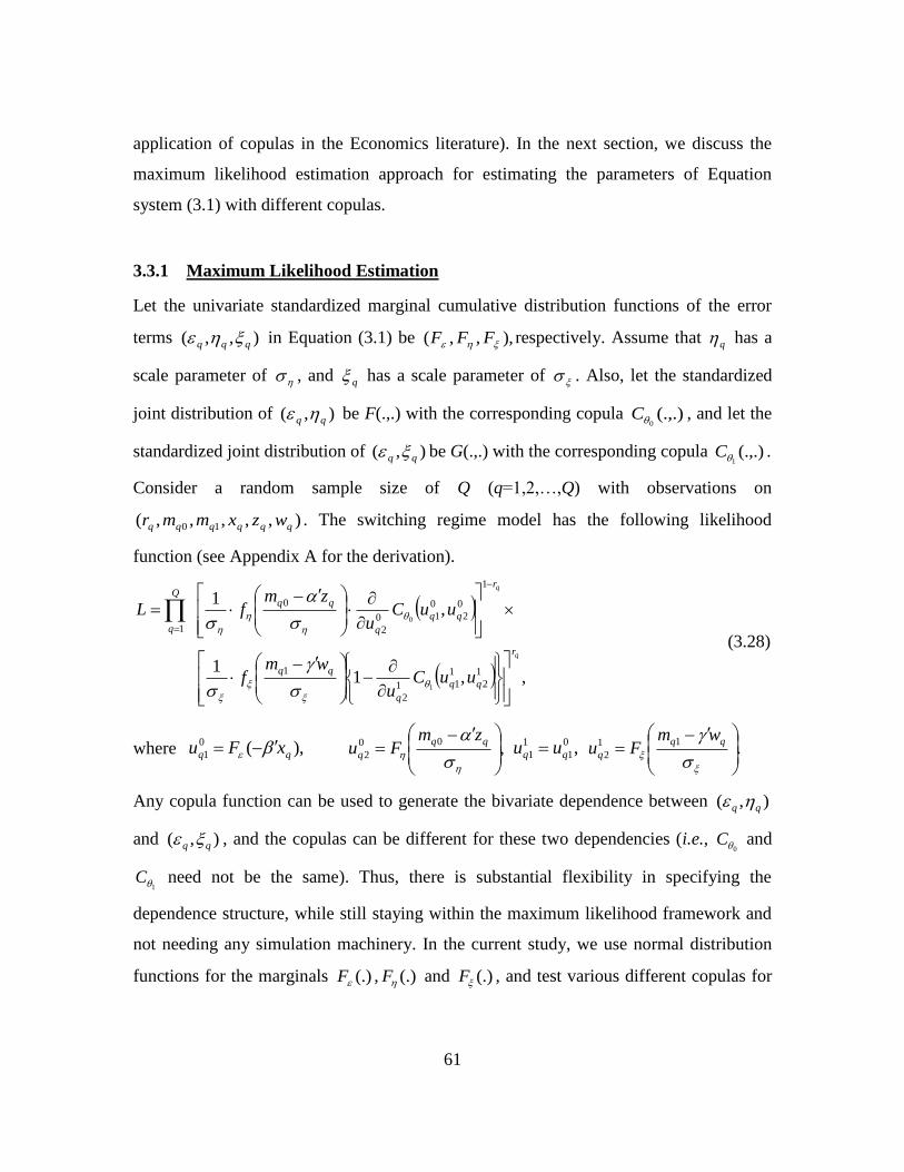
61
application of copulas in the Economics literature). In the next section, we discuss the
maximum likelihood estimation approach for estimating the parameters of Equation
system (3.1) with different copulas.
3.3.1 Maximum Likelihood Estimation
Let the univariate standardized marginal cumulative distribution functions of the error
terms ),,( qqq in Equation (3.1) be ),,,( FFF respectively. Assume that q has a
scale parameter of , and q has a scale parameter of . Also, let the standardized
joint distribution of ),( qq be F(.,.) with the corresponding copula (.,.)0
C , and let the
standardized joint distribution of ),( qq be G(.,.) with the corresponding copula (.,.)1
C .
Consider a random sample size of Q (q=1,2,…,Q) with observations on
),,,,,( 10 qqqqqq wzxmmr . The switching regime model has the following likelihood
function (see Appendix A for the derivation).
,,11
,1
1
2
1
11
2
1
1
0
2
0
10
2
0
1
1
0
q
q
r
q
r
q
qqQ
q
uuCu
wmf
uuCu
zmfL
(3.28)
where ),(0
1 qq xFu ,
00
2
q
zmFu ,0
1
1
1 qq uu .11
2
q
wmFu
Any copula function can be used to generate the bivariate dependence between ),( qq
and ),( qq , and the copulas can be different for these two dependencies (i.e., 0
C and
1C need not be the same). Thus, there is substantial flexibility in specifying the
dependence structure, while still staying within the maximum likelihood framework and
not needing any simulation machinery. In the current study, we use normal distribution
functions for the marginals (.)F , (.)F and (.)F , and test various different copulas for
62
0C and
1C . In Table 3.2, we provide the expression for ),( 21
2
uuCu
for the six
copulas discussed in Section 3.2.3. For Archimedean copulas, the expression has the
simple form provided in Equation (3.19).
The maximum-likelihood estimation of the sample selection model with different
copulas leads to a case of non-nested models. The most widely used approach to select
among the competing non-nested copula models is the Bayesian Information Criterion (or
BIC; see Quinn, 2007, Genius and Strazzera, 2008, Trivedi and Zimmer, 2007, page 65).
The BIC for a given copula model is equal to )ln()ln(2 QKL , where )ln(L is the log-
likelihood value at convergence, K is the number of parameters, and Q is the number of
observations. The copula that results in the lowest BIC value is the preferred copula. But,
if all the competing models have the same exogenous variables and a single copula
dependence parameter θ, the BIC information selection procedure measure is equivalent
to selection based on the largest value of the log-likelihood function at convergence.
3.4 Data
3.4.1 Data sources
The data used for this analysis is drawn from the 2000 San Francisco Bay Area
Household Travel Survey (BATS) designed and administered by MORPACE
International Inc. for the Bay Area Metropolitan Transportation Commission (MTC). In
addition to the 2000 BATS data, several other secondary data sources were used to derive
spatial variables characterizing the activity-travel and built environment in the region.
These included: (1) Zonal-level land-use/demographic coverage data, obtained from the
MTC, (2) GIS layers of sports and fitness centers, parks and gardens, restaurants,
recreational businesses, and shopping locations, obtained from the InfoUSA business
directory, (3) GIS layers of bicycling facilities, obtained from MTC, and (4) GIS layers
of the highway network (interstate, national, state and county highways) and the local
roadways network (local, neighborhood, and rural roads), extracted from the Census 2000
Tiger files. From these secondary data sources, a wide variety of built environment

63
variables were developed for the purpose of classifying the residential neighborhoods
into neo-urbanist and conventional neighborhoods.
3.4.2 The Dependent Variables
This study uses factor analysis and a clustering technique to define a binary residential
location variable that classifies the Traffic Analysis Zones (TAZs) of the Bay Area into
neo-urbanist and conventional neighborhoods based on built environment measures.
Factor analysis helps in reducing the correlated attributes (or factors) that characterize the
built environment of a neighborhood into a manageable number of principal components
(or variables). The clustering technique employs these principal components to classify
zones into neo-urbanist or conventional neighborhoods. In the current study, we employ
the results from Pinjari et al. (2008) that identified two principal components to
characterize the built environment of a zone - (1) Residential density and
transportation/land-use environment, and (2) Accessibility to activity centers. The factors
loading on the first component included bicycle lane density, number of zones accessible
from the home zone by bicycle, street block density, household population density, and
fraction of residential land use in the zone. The factors loading on the second component
included bicycle lane density and number of physically active and natural recreation
centers in the zone. The two principal components formed the basis for a cluster analysis
that categorizes the 1099 zones in the Bay area into neo-urbanist or conventional
neighborhoods (see Pinjari et al., 2008 for complete details). This binary variable is used
as the dependent variable in the selection equation of Equation (3.1).
The continuous outcome dependent variable in each of the neo-urbanist and conventional
neighborhood residential location regimes is the household vehicle miles of travel
(VMT). This was obtained from the reported odometer readings before and after the two
days of the survey for each vehicle in the household. The two-day vehicle-specific VMT
was aggregated across all vehicles in the household to obtain a total two-day household
VMT, which was subsequently averaged across the two survey days to obtain an average
daily household VMT. The logarithm of the average daily household VMT was then used
64
as the dependent variable, after recoding the small share (<5%) of households with a
VMT value of zero to one (so that the logarithm of VMT takes a value of zero for these
households).
The final estimation sample in our analysis includes 3696 households from 5
counties (San Francisco, San Mateo, Santa Clara, Alameda, and Contra Costa) of the Bay
area. Among these households, about 34% of the households reside in neo-urbanist
neighborhoods and 66% reside in conventional neighborhoods. The average daily
household VMT is about 37 miles for households in neo-urbanist neighborhoods, and 68
miles for households in conventional neighborhoods.
3.5 Empirical analysis
3.5.1 Variables considered
Several categories of variables were considered in the analysis, including household
demographics, employment characteristics, and neighborhood characteristics. The
neighborhood characteristics considered include population density, employment density,
Hansen-type accessibility measures (such as accessibility to employment and
accessibility to shopping; see Bhat and Guo, 2007 for the precise functional form),
population by ethnicity in the neighborhood, presence/number of schools and physically
active centers, and density of bicycle lanes and street blocks. These measures are
included in the VMT outcome equation and capture the effect of variations in built
environment across zones within each group of neo-urbanist and conventional
neighborhoods.
3.5.2 Estimation Results
The empirical analysis involved estimating models with the same structure for ),( qq
and ),( qq , as well as different copula-based dependency structures. This led to 6
models with the same copula dependency structure (corresponding to the six copulas
discussed in Section 3.2.3), and 24 models with different combinations of the six copula
65
dependency structures for ),( qq and ),( qq . We also estimated a model that
assumed independence between q and q , and q and q .
The Bayesian Information Criterion, which collapses to a comparison of the log-
likelihood values across different models, is employed to determine the best copula
dependency structure combination. The log-likelihood values for the five best copula
dependency structure combinations are: (1) Frank-Frank (-6842.2), (2) Frank-Joe (-
6844.2), (3) FGM-Joe (-6851.0), (4) Independent-Joe (-6863.7), and (5) FGM-Gumbel (-
6866.2). It is evident that the log-likelihood at convergence of the Frank-Frank and
Frank-Joe copula combinations are higher compared to the other copula combinations.
Between the Frank-Frank and Frank-Joe copula combinations, the former is slightly
better. The log-likelihood value for the structure that assumes independence (i.e., no self-
selection effects) is -6878.1. All the five copula-based dependency models reject the
independence assumption at any reasonable level of significance, based on likelihood
ratio tests, indicating the significant presence of self-selection effects. Interestingly,
however, the log-likelihood value at convergence for the classic textbook structure that
assumes a Gaussian-Gaussian copula combination is -6877.9, indicating that there is no
statistically significant difference between the Gaussian-Gaussian (G-G) and the
independence-independence (I-I) copula structures. This is also observed in the estimated
bivariate normal correlation parameters, which are -0.020 (t-statistic of 0.18) for the
residential choice-neo-urbanist VMT regime error correlation and -0.050 (t-statistic of -
0.50) for the residential choice-conventional neighborhood VMT regime error
correlation. Clearly, the traditional G-G copula combination indicates the absence of self-
selection effects. However, this is simply an artifact of the normal dependency structure,
and is indicative of the kind of incorrect results that can be obtained by placing restrictive
distributional assumptions.
In the following presentation of the empirical results, we focus our attention on
the results of the Independent-Independent (or I-I copula) specification that ignores self-
selection effects entirely and the Frank-Frank (or F-F copula) specification that provides
the best data fit. Table 3.3 provides the results, which are discussed below.

66
3.5.2.1 Binary choice component
The results of the binary discrete equation of neighborhood choice provide the effects of
variables on the propensity to reside in a conventional neighborhood relative to a neo-
urbanist neighborhood. The parameter estimates indicate that younger households (i.e.,
households whose heads are less than 35 years of age) are less likely to reside in
conventional neighborhoods and more likely to reside in neo-urbanist neighborhoods,
perhaps because of higher environmental sensitivity and/or higher need to be close to
social and recreational activity opportunities (see also Lu and Pas, 1999). Households
with children have a preference for conventional neighborhoods, potentially because of a
perceived better quality of life/schooling for children in conventional neighborhoods
compared to neo-urbanist neighborhoods. Also, as expected, households who own their
home and who live in a single family dwelling unit are more likely to reside in
conventional neighborhoods.
3.5.2.2 Log(VMT) continuous component for neo-urbanist neighborhood regime
The estimation results corresponding to the natural logarithm of vehicle miles of travel
(VMT) in a neo-urbanist neighborhood highlight the significance of the number of
household vehicles and number of full-time students. As expected, both of these effects
are positive. In particular, log(VMT) increases with number of vehicles in the household
and number of students. The effect of number of vehicles is non-linear, with a jump in
log(VMT) for an increase from no vehicles to one vehicle, and a lesser impact for an
increase from one vehicle to 2 or more vehicles (there were only two households in neo-
urbanist neighborhoods with 3 vehicles, so we are unable to estimate impacts of vehicle
increases beyond 2 vehicles in neo-urbanist neighborhoods). Interestingly, we did not
find any statistically significant effect of employment and neighborhood characteristics,
in part because the variability of these characteristics across households in neo-urbanist
zones is relatively small.
67
The copula dependency parameter between the discrete choice residence error
term and the log(VMT) error term for neo-urbanist households is highly statistically
significant and negative for the F-F model. The estimate translates to a Kendall‟s
value of -0.26. The negative dependency parameter indicates that a household that has a
higher inclination to locate in conventional neighborhoods would travel less than an
observationally equivalent “random” household if both these households were located in
a neo-urbanist neighborhood (a “random” household, as used above, is one that is
indifferent between residing in a neo-urbanist or a conventional neighborhood, based on
factors unobserved to the analyst). Equivalently, the implication is that a household that
makes the choice to reside in a neo-urbanist neighborhood is likely to travel more than an
observationally equivalent random household in a neo-urbanist environment, and much
more than if an observationally equivalent household from a conventional neighborhood
were relocated to a neo-urbanist neighborhood. This may be attributed to, among other
things, such unobserved factors characterizing households inclined to reside in neo-
urbanist settings as a higher degree of comfort level driving in dense, one-way street-
oriented, parking-loaded, traffic conditions.
The lower travel tendency of a random household in a neo-urbanist neighborhood
(relative to a household that expressly chooses to locate in a neo-urbanist neighborhood)
is teased out and reflected in the high statistically significant negative constant in the F-F
copula model. On the other hand, the I-I model assumes, incorrectly, that the travel of
households choosing to reside in neo-urbanist neighborhoods is independent of the choice
of residence. The result is an inflation of the VMT generated by a random household if
located in a neo-urbanist setting.
3.5.2.3 Log(VMT) continuous component for conventional neighborhood regime
The household socio-demographics that influence vehicle mileage for households in a
conventional neighborhood include number of household vehicles, number of full-time
students, and number of employed individuals. As expected, the effects of all of these
variables are positive. The household vehicle effect is non-linear, with the marginal
68
increase in log(VMT) decreasing with the number of vehicles. In addition, two
neighborhood characteristics – density of vehicle lanes and accessibility to shopping –
have statistically significant effects on log(VMT) in the conventional neighborhood
regime. Both these effects are negative, as expected.
The dependency parameter in this segment for the F-F model is highly statistically
significant and positive. The estimate translates to a Kendall‟s value of 0.36. The
positive dependency indicates that a household that has a higher inclination to locate in
conventional neighborhoods is likely to travel more in that setting than an observationally
equivalent random household. Again, the I-I model ignores this residential self-selection
in the estimation sample, resulting in an over-estimation of the VMT generated by a
random household if located in a conventional neighborhood setting (see the higher
constant in the I-I model relative to the F-F model corresponding to the conventional
neighborhood VMT regime).
3.6 Summary
In the current study, we apply a copula based approach to model residential neighborhood
choice and daily household vehicle miles of travel (VMT) using the 2000 San Francisco
Bay Area Household Travel Survey (BATS). The self-selection hypothesis in the current
empirical context is that households select their residence locations based on their travel
needs, which implies that observed VMT differences between households residing in
neo-urbanist and conventional neighborhoods cannot be attributed entirely to built
environment variations between the two neighborhoods types. A variety of copula-based
models are estimated, including the traditional Gaussian-Gaussian (G-G) copula model.
The results indicate that using a bivariate normal dependency structure suggests the
absence of residential self-selection effects. However, other copula structures reveal a
high and statistically significant level of residential self-selection, highlighting the
potentially inappropriate empirical inferences from using incorrect dependency
structures. In the current empirical case, we find the Frank-Frank (F-F) copula
69
dependency structure to be the best in terms of data fit based on the Bayesian Information
Criterion.
The copula approach used here can be extended to the case of sample selection
with a multinomial treatment effect. In the subsequent chapter we extend the copula
approach for multinomial context (see also Spizzu et al., 2009, for a similar application).
It should also have wide applicability in other bivariate/multivariate contexts in the
transportation and other fields, including spatial dependence modeling (see Bhat and
Sener, 2009).
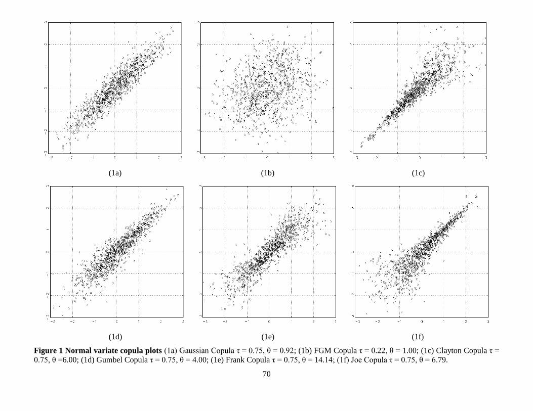
70
(1a) (1b) (1c)
(1d) (1e) (1f)
Figure 1 Normal variate copula plots (1a) Gaussian Copula τ = 0.75, θ = 0.92; (1b) FGM Copula τ = 0.22, θ = 1.00; (1c) Clayton Copula τ =
0.75, θ =6.00; (1d) Gumbel Copula τ = 0.75, θ = 4.00; (1e) Frank Copula τ = 0.75, θ = 14.14; (1f) Joe Copula τ = 0.75, θ = 6.79.
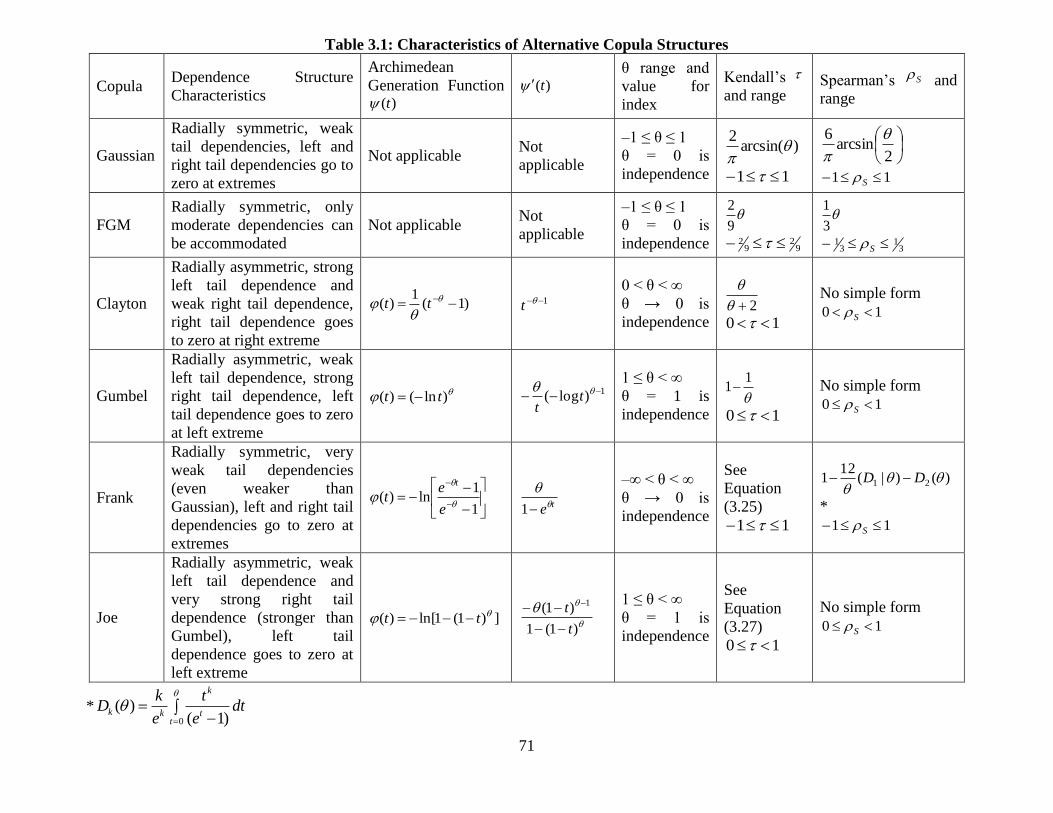
71
Table 3.1: Characteristics of Alternative Copula Structures
Copula Dependence Structure
Characteristics
Archimedean
Generation Function )(t
)(t
θ range and
value for
index
Kendall‟s
and range Spearman‟s S and
range
Gaussian
Radially symmetric, weak
tail dependencies, left and
right tail dependencies go to
zero at extremes
Not applicable Not
applicable
–1 ≤ θ ≤ 1
θ = 0 is
independence
)arcsin(2
11
2arcsin
6
11 S
FGM
Radially symmetric, only
moderate dependencies can
be accommodated
Not applicable Not
applicable
–1 ≤ θ ≤ 1
θ = 0 is
independence
9
2
9
29
2
3
1
3
13
1 S
Clayton
Radially asymmetric, strong
left tail dependence and
weak right tail dependence,
right tail dependence goes
to zero at right extreme
)1(1
)(
tt
1t
0 < θ < ∞
θ → 0 is
independence 2
10
No simple form
10 S
Gumbel
Radially asymmetric, weak
left tail dependence, strong
right tail dependence, left
tail dependence goes to zero
at left extreme
)ln()( tt 1)log(
tt
1 ≤ θ < ∞
θ = 1 is
independence
11
10
No simple form
10 S
Frank
Radially symmetric, very
weak tail dependencies
(even weaker than
Gaussian), left and right tail
dependencies go to zero at
extremes
1
1ln)(
e
et
t
te
1
–∞ < θ < ∞
θ → 0 is
independence
See
Equation
(3.25)
11
)()|(12
1 21
DD
*
11 S
Joe
Radially asymmetric, weak
left tail dependence and
very strong right tail
dependence (stronger than
Gumbel), left tail
dependence goes to zero at
left extreme
])1(1ln[)( tt
)1(1
)1( 1
t
t
1 ≤ θ < ∞
θ = 1 is
independence
See
Equation
(3.27)
10
No simple form
10 S
*0
( )( 1)
k
k k tt
k tD dt
e e
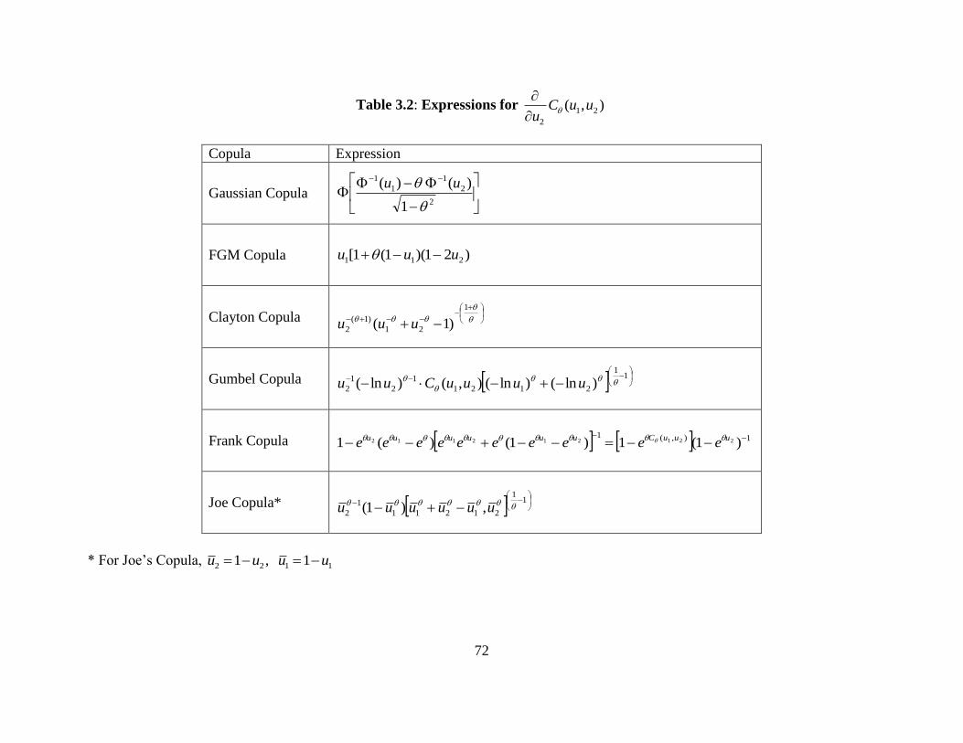
72
Table 3.2: Expressions for 1 2
2
( , )C u uu
Copula Expression
Gaussian Copula
2
2
1
1
1
1
)( )(
uu
FGM Copula )21)(1(1[ 211 uuu
Clayton Copula
1
21
)1(
2 )1( uuu
Gumbel Copula
1
1
2121
1
2
1
2 )ln()ln(),()ln(
uuuuCuu
Frank Copula 1),(1)1(1)1()(1 221212112
uuuCuuuuuu
eeeeeeeeee
Joe Copula*
11
21211
1
2 ,)1( uuuuuu
* For Joe‟s Copula, 2 2 1 11 , 1u u u u
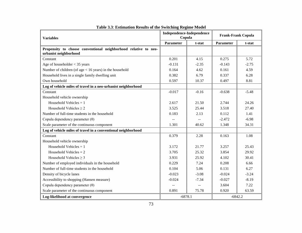
73
Table 3.3: Estimation Results of the Switching Regime Model
Variables
Independence-Independence
Copula Frank-Frank Copula
Parameter t-stat Parameter t-stat
Propensity to choose conventional neighborhood relative to neo-
urbanist neighborhood
Constant 0.201 4.15 0.275 5.72
Age of householder < 35 years -0.131 -2.35 -0.143 -2.75
Number of children (of age < 16 years) in the household 0.164 4.62 0.161 4.59
Household lives in a single family dwelling unit 0.382 6.79 0.337 6.28
Own household 0.597 10.37 0.497 8.81
Log of vehicle miles of travel in a neo-urbanist neighborhood
Constant -0.017 -0.16 -0.638 -5.48
Household vehicle ownership
Household Vehicles = 1 2.617 21.50 2.744 24.26
Household Vehicles ≥ 2 3.525 25.44 3.518 27.40
Number of full-time students in the household 0.183 2.13 0.112 1.41
Copula dependency parameter (θ) -- -- -2.472 -6.98
Scale parameter of the continuous component 1.301 40.62 1.348 34.31
Log of vehicle miles of travel in a conventional neighborhood
Constant 0.379 2.28 0.163 1.08
Household vehicle ownership
Household Vehicles = 1 3.172 21.77 3.257 25.43
Household Vehicles = 2 3.705 25.32 3.854 29.92
Household Vehicles ≥ 3 3.931 25.92 4.102 30.41
Number of employed individuals in the household 0.229 7.24 0.208 6.66
Number of full-time students in the household 0.104 5.06 0.131 6.27
Density of bicycle lanes -0.023 -3.08 -0.024 -3.24
Accessibility to shopping (Hansen measure) -0.024 -7.34 -0.027 -8.19
Copula dependency parameter (θ) -- -- 3.604 7.22
Scale parameter of the continuous component 0.891 75.78 0.920 63.59
Log-likelihood at convergence -6878.1 -6842.2
74
CHAPTER 4 HOUSEHOLD VEHICLE FLEET COMPOSITION
AND USAGE CHOICES
4.1 Introduction and literature
This chapter focuses on understanding the effects of land use measures on vehicle
ownership by type of vehicle and usage. Understanding the interaction between land use
and travel behavior has been of much interest to the profession, with a long history and
strand of literature devoted to this subject (e.g., Ewing and Cervero 2001, Lund 2003,
Song and Knaap 2003, Bhat and Eluru 2009). There are descriptive studies that compare
travel behavior characteristics of households and individuals residing in low density land
use configurations against those that reside in higher density mixed land use
configurations. There are studies that consider the impacts of residential location
characteristics on a host of travel behavior characteristics including, for example, mode
choice (Pinjari et al., 2007, Chen et al., 2008), auto ownership (Bhat and Guo, 2007),
vehicle miles of travel, activity time use patterns (Pinjari et al., 2009) and amount of non-
motorized travel (Pinjari et al., 2008). Thus, the interplay between land use and travel
behavior remains a major focus area of research in the profession and continues to be of
much interest particularly in the context of developing integrated land use-transport
models that effectively model the impacts of alternative land use strategies on travel
demand.
In recent years, there has been an explicit recognition in the integrated land use-
transport modeling field that the treatment of residential land use characteristics as
exogenous factors (variables) in models of vehicle ownership and use (or any travel
behavior model) may provide erroneous indications of the true impacts of land use on
travel behavior. This is due to the phenomenon referred to as “self-selection” where
households or individuals who have a proclivity towards a certain lifestyle may choose or
“self-select” to reside in neighborhoods that support their lifestyle preferences. People‟s
attitudes, preferences, and values, not to mention their socio-economic and demographic
characteristics, undoubtedly play a role in shaping behavioral choices (Bhat and Guo
75
2007, Choo and Mokhtarian 2004, Cao et al., 2006, Handy 2005). If an individual who
tends to be environmentally conscious and enjoys a non-motorized travel lifestyle
characterized by bicycling and walking chooses to reside in a high-density mixed land
use development, it is likely that the residential location choice was influenced by the
lifestyle and travel preferences of the individual (as opposed to the travel choices being
driven by the land use pattern of the residential location). In other words, residential
location choice is endogenous to vehicle ownership choice by vehicle type, vehicle usage
decisions, and other travel behavior choices that are made by individuals and households
in which they reside.
In light of the key role that vehicle ownership, vehicle type choice, and vehicle
usage have played in travel demand analysis over many decades, and in the global
climate change debate more recently, there has been considerable research the
determinants of vehicle ownership, household fleet composition (vehicle type mix), and
vehicle usage (usually measured in vehicle miles of travel). Work in this area has ranged
from simple regression or discrete choice models of levels of auto ownership (e.g.,
Mannering and Winston 1985) and vehicle type choice (Feng et al., 2005, Goldberg
1998, Mohamaddian and Miller 2003) to more sophisticated models of vehicle
acquisition, disposal, and replacement (Yamamoto et al., 1999). More recently, there has
been considerable work on modeling household fleet composition in terms of the mix of
vehicle types owned by a household together with the amount that each vehicle in the
household is used. But these models often treat residential location choice variables (land
use measures) as exogenous variables that influence vehicle fleet ownership and usage
(e.g., Shay and Khattak 2005, Bhat et al., 2009). Further, many of these earlier studies
consider the jointness in vehicle type choice and usage for the most recent vehicle or
most driven by the household [for example, see Choo and Mokhtarian 2004,
Mohammadian and Miller 2003, Spissu et al. 2009], or confine their attention to
households with two or fewer vehicles [see West 2004]. Overall, there has been relatively
little research on treating residential choice as being endogenous in vehicle type and
76
usage decisions, or on examining the entire vehicle fleet composition and usage
characteristics of households.
This chapter contributes to the literature on land use and travel demand by
explicitly integrating household vehicle ownership, vehicle type, and vehicle usage
decisions with residential location decisions of households. Such a joint model can be
used to conduct a host of policy analyses aimed at reducing GHG emissions and fuel
consumption. The joint model system is estimated on a data set derived from the 2000
San Francisco Bay Area Household Travel Survey (BATS) that has been
comprehensively augmented with land use and network level of service attributes. The
chapter starts with a presentation of the methodology in the next section. A brief
description of the data is offered in the third section. The fourth section presents model
estimation results while the fifth section offers a discussion on the simultaneity in the
choice processes. Concluding thoughts are offered in the sixth section.
4.2 Modeling methodology
In this section, the model framework to jointly model residential location, vehicle
ownership and type choice, and vehicle usage, is discussed first followed by a detailed
presentation of the model structure and model estimation procedure.
4.2.1 Model framework
The number of dimensions that need to be modeled in the joint residential choice and
vehicle fleet composition/usage system is high, especially because of the consideration of
multiple vehicles in the household. One appealing approach to accommodating the high
number of dimensions due to multiple vehicles is to consider a multiple discrete-
continuous extreme value (MDCEV) based model, as undertaken by Bhat et al. 2009.
The approach is quite elegant and relatively simple, but, when applied to vehicle fleet
composition analysis, is predicated on the assumption that the process of acquiring
vehicles is instantaneous and based on “horizontal” choice behavior. The basic
supposition is that, at a given instant, individuals choose to purchase the number of
77
vehicles they want to own as well as the vehicle type and use decisions. However, it is
more reasonable to assume that the fleet ownership of households is based on repeated
choice decisions over time, with the choices made at an earlier occasion influencing
future choices. The MDCEV approach is fundamentally at odds with this more realistic
process of household vehicle ownership and use. Further, the MDCEV approach ties the
discrete and continuous choices in a restrictive framework by having a single stochastic
utility function (and therefore, a single error term) that underlies both the discrete and
continuous choices. Finally, the MDCEV approach needs to have an exogenous total
mileage budget of households for implementation. Bhat et al. 2009 develop this budget
by aggregating the mileage across all vehicles held by a household and adding non-
motorized mode mileage. However, the non-motorized mileage is a relatively negligible
fraction of total mileage, effectively imposing the constraint that total motorized vehicle
utilization is exogenous, and does not change in response to policies or fuel cost increases
(though the MDCEV model allows substitution in vehicle mileage across different
vehicle types).
In the current study, a different approach is adopted to accommodate the many
dimensions characterizing vehicle fleet/usage decisions. Multiple vehicle ownership and
usage dimensions are accommodated by assuming that vehicle fleet and usage decisions
are determined through a series of unobserved (to the analyst) repeated discrete-
continuous choice occasions [see Hendel 1999 and Dube 2004, who have earlier used a
repeated choice framework to handle the purchase and consumption levels of multiple
items in a marketing context]. The number of choice occasions in such a “vertical” choice
behavior is linked to the number of adults in the household. In particular, since the
number of vehicles is never greater than the number of adults in the household plus 1 in
the data used in this empirical context, the number of choice occasions is set to be equal
to the number of adults plus 1. At each choice occasion, the household may choose not to
purchase a vehicle or to acquire a vehicle of a certain type. However, the choice of
residential location, vehicle ownership, vehicle type and vehicle utilization are likely to
be multiple dimensions of a single choice bundle at each choice occasion. For example, a
78
household that is environmentally conscious may deliberately decide to locate in a neo-
urbanist neighborhood, have few cars (as reflected in the choice of zero cars on one or
more choice occasions of the household), favor compact vehicles in each choice
occasion, and use the chosen vehicles relatively sparingly. This joint nature of the
decisions is recognized at each choice occasion by proposing a joint discrete-continuous
copula-based framework [the use of a copula framework is a deviation from earlier
modeling approaches of repeated discrete-continuous choices, including those of Dube
2004 and Bento et al. 2005]. In the framework, the decision of residential choice, and
choice of no vehicle purchase or one of several vehicle types, is captured using a GEV-
based logit model, while vehicle utilization (as measured by annual vehicle miles of
travel or VMT) of the chosen vehicle type is modeled using a continuous regression
model. Note that one can use this framework to model any representation of residential
choice (such as neo-urbanist versus traditional neighborhoods as in Bhat and Eluru 2009
or multiple residential choice alternatives based on density as in Brownstone and Golob
2009 and any taxonomy of vehicle types. Also important is that the number of vehicles
owned by the household is endogenously, even if implicitly, determined as the sum of
those choice occasions when the household selects a certain vehicle type. Overall, the
proposed approach jointly models residential choice and all vehicle fleet characteristics in
a unifying framework.
To implement this framework in estimation, “synthetic” repeated choice
occasions for each household are generated based on the number of adults in the
household. Appropriate vehicle type choices are assigned to each choice occasion in the
estimation sample. For example, consider a household with two adults, and two vehicles
– a coupe and a compact sedan. For this household, three choice occasions (2 adults +1)
are created with the chosen alternatives for the choice occasions being coupe, compact
sedan and “no vehicle”. In the data set used in the empirical analysis part of this study,
the temporal sequence of the purchase of the vehicles currently owned is known. Thus, it
is possible to capture the impacts of the types of vehicles already owned on the type of
vehicle that may be purchased in a subsequent purchase decision. In the example above,
79
if the coupe is the first vehicle purchased and the sedan is the second one purchased,
coupe is assigned as the chosen alternative at the first choice occasion, and sedan as the
chosen alternative in the second. In the second choice occasion, information that the
household has a coupe is used as an explanatory variable. This “mimics” the dynamics of
fleet ownership decisions.7
4.2.2 Model Structure
4.2.2.1 Joint Residential Location-Vehicle Type Choice Model Component (Discrete
Choice Component)
Let q be the index for households, ( = 1, 2, ..., )q Q and let i be the index for the
possible combinations of residential location alternatives and vehicle type alternatives.
For example, if residential location is characterized by two alternatives (residing in a neo-
urbanist neighborhood and residing in a traditional neighborhood) and vehicle type is
represented by three alternatives (no vehicle purchased, sedan, and coupe; for ease in
presentation, the “no vehicle” purchased case will be treated as a vehicle type
alternative), there are 6 possible combinations of residential location and vehicle type
alternatives, and i = 1, 2, 3, 4, 5, 6. More generally, let i = 1, 2, …, I. Also, let j be the
index to represent the vehicle choice occasion ( 1, 2, ... ,j J where J is the number of
adults in the household q plus 1). With this notation, the residential location-vehicle type
discrete choice model component takes the familiar random utility formulation:
* 'qij qij qiju x (4.1)
In the equation above, *qij
u is the latent utility that the thq household derives from
choosing alternative i at the jth
choice occasion. qijx is a column vector of known
7 Note that in the example just provided, one could also assign the chosen alternatives to the choice
occasions as follows: coupe in first choice occasion, no vehicle in the second, and sedan in the third. This is
in place of coupe in the first, sedan in the second and no vehicle in the third. But both these assignments
will give the same results, because the “dynamics” are based on what the household already owns in
totality, not what was chosen in the immediately previous choice occasion. Of course, for the first choice
occasion, there are no explanatory variables related to the vehicle types already chosen, because there is no
information on what the household owned prior to the set of vehicles currently held.
80
household attributes at choice occasion j (including household demographics, types of
vehicles “chosen” before the jth
choice occasion, and activity-travel environment
characteristics), is a corresponding coefficient column vector of parameters to be
estimated, and qij is an idiosyncratic error term assumed to be standard type-1 extreme
value distributed. Then, in the usual framework of random utility maximization,
household q will choose alternative i at the jth
choice occasion if the following condition
holds:
1,2,..., ,
* *maxs I s i
qij qsju u
(4.2)
The condition above can be equivalently written in the form of a series of binary
choice formulations for each alternative i [see Lee 1983]. To see this, let qij
R be a
dichotomous variable that takes the values 0 and 1, with 1qij
R if the thi alternative is
chosen by the thq household at the jth
choice occasion, and 0qij
R otherwise. Then,
one can recast the discrete choice model formulation in Equation (4.2) by substituting
'qij qijx for *
qiju [from Equation (4.1)]:
,1 if ( 1,2,... )qij'
qijqijR x v i I (4.3)
1,2,..., ,
*where { max }s I s i
qij qsj qijv u
(4.4)
With the structure in Equation (4.4) and an appropriate Generalized Extreme
Value (GEV) distribution assumption on the qij terms, the residential location-vehicle
type choice probability expressions at each choice occasion j take the usual GEV form
[see McFadden 1978]. In the model, it is assumed that the error terms qij are
independent and identically distributed (IID) across households q and choice occasions j,
and that they are identically distributed (but not necessarily independent) across
81
alternatives i.8 Let (.)viF be the marginal distribution of qijv implied by the assumed GEV
distributional form for the qij terms and the relationship in Equation (4.4). This implied
distribution is very straightforward to obtain, since it is based on the probability
expression for the corresponding discrete choice model. For example, if the qij terms are
independent across alternative i, then, from Equation (4.3), it must be the case that:
is
qsjqij
qij
qijqijvixx
xxvF
)exp()exp(
)exp()(
, and therefore
exp( )( )
exp( ) exp( )vi qij qij
qsjs i
wF v x
w x
If some other GEV form is used for the qij terms, then the implied distribution
of qijv will take the corresponding GEV probability form.
4.2.2.2 The Vehicle Mileage Model Component
In the current modeling framework, the vehicle mileage model component takes the form
of the classic log-linear regression, as shown below:
* *, 1[ 1]qij qij qij qij'
qijqijm z m R m (4.5)
In the equation above, *qijm is a latent variable representing the logarithm of annual
mileage on the vehicle of type i if it had been chosen at the jth
choice occasion. This
latent vehicle usage variable is mapped to the observed household attributes and the
corresponding attribute effects in the form of column vectors qijz and ' , respectively,
as well as to unobserved factors through a qij term. On the right hand side of this
equation, the notation 1[ 1]qijR represents an indicator function taking the value 1 if
8 The IID assumptions across households and choice occasions can be relaxed in a conceptually
straightforward manner by accommodating mixing distributions. This is left for future research, and focus
in the current paper on implementing the fundamental “vertical” choice approach.
82
household q chooses vehicle type i in the jth
choice occasion, and 0 otherwise. That is,
*qijm is observed (in the form of
qijm ) only if household q is observed to actually
acquire a vehicle of type i at the jth
choice occasion. It is assumed that the qij error terms
are independent and identically distributed (IID) across households q and choice
occasions j, and that they are identically distributed (but not necessarily independent)
across alternatives i. Further, since the annual mileage for the chosen vehicle is only
observed at each choice occasion, any dependence between the qij terms across
alternatives i is not identified.
4.2.2.3 The Joint Model: A Copula-based Approach
In this sub-section, the specifications of the individual model components discussed in
the previous two subsections are brought together in the following equation system:
* *
,1 if ( 1, 2, ... ) ( 1, 2, ... )
, 1[ 1]
qij
'qij i qij
'qij i qij qij qij qij qij
R x i I j J
m z m R m
v
(4.6)
The type and the extent of the dependency between the stochastic terms qijv and
qij for household q determines the level of dependency between the underlying
propensity of vehicle type choice and vehicle usage decisions for the household. In the
research effort, as indicated earlier, copula-based methods are used to capture and explore
these dependencies (or correlations). In particular, copulas are used to describe the joint
distribution of the qijv and qij terms. In this approach, first, the qijv and qij terms are
transformed into uniform distributions using their inverse cumulative distribution
functions. Subsequently, copulas are applied to “couple” the uniformly distributed
inverse cumulative distributions into multivariate joint distributions. To explicate, lets
assume that the marginal distributions of qijv and qij be (.)viF and (.)iF , respectively,
and let the joint distribution of qijv and qij be ,
(., .)vi i
F
.
83
Subsequently, consider, 1 2
( , ),vi i
F y y
which can be expressed as a joint
cumulative probability distribution of uniform [0,1] marginal variables 1
U and 2
U as
below:
1 2
1 11 21 2
1 21 2
, 1 2( , ) P( , )
P( ( ) , ( ) )
P( ( ), ( ))
qij qijvi i
vi i
vi i
F y y y y
F U y F U y
U F y U F y
v
(4.7)
Then, the above joint distribution (of uniform marginal variables) can be
generated by a function (., .)C
such that (Sklar 1973):
1 21 2, 1 2
( , ) ( ( ), ( ))vi i vi i
F y y u F y u F yC
(4.8)
where (., .)C
is a copula function and is a dependency parameter (assumed to be
scalar), together characterizing the dependency between qijv and qij . The joint
distribution formed in the above-discussed manner is used to derive the joint residential
location, and vehicle ownership and type combination choice, and vehicle mileage
probabilities and log-likelihood expressions.
4.2.3 Model estimation
The joint model based on the formulation above has the following log-likelihood
expression for a random sample of Q households ( = 1, 2, ..., )q Q :
( * )|
1 1 1
Q J I RqijR H' 'qij qjx xqij qij qij qij qijq j i
L P m P
. (4.9)
where Hqj = 1 if it is not the case that the household q chooses no vehicles at choice
occasion j, and 0 otherwise.
The conditional distributions in the above expression can be expressed as:

84
1
1
1
,
, '
1 2
2
'' ' '| ,
1' ' ,
1'
, '
qij qij
i
i
m zt
i
i
qij qijqij qij qijvi i
qi
vi i
i ii q q qij qij
iiq
m zP m x v P x v F xqij qij qij
m
P x v F x tqij qij qijt
C u u m zP x v fqij qij
u
i
(4.10)
where (., .)iC is the copula corresponding to 1 2,( , )i i
q qvi iF u u
with 1 ( )i '
q vi i qiju F x
and 2
'qij i qij
i
ziq i
mu F
, 1 2
2
,i ii q q
iq
C u u
u
is the partial derivative of the copula
with respect to 2iqu [see Bhat and Eluru (4)], if is the probability density function of
qij , and i
is the scale parameter of qij .
Substitution of the above conditional distribution expression back into Equation
(4.10) provides the following log-likelihood expression for the joint residential location,
and vehicle ownership and type combination choice, and vehicle usage model:
, (1 )1 2 '*1 1 1 2
( * )'
1qij qji iuQ zJ I i Hq q qij qij qj
P xi qij qijiuq j i i iq
R HC u m
L f
(4.11)
A particular advantage of the copula-based approach is that, in the above log-
likelihood expression, several different copula [i.e., (., .)iC ] functions can be explored to
characterize the dependency between the residential location-vehicle type choice discrete
component and the continuous vehicle miles of travel (VMT) component [see Chapter 3
for a review of alternative copula functions available in the literature]. Specifically, the
copula approach allows us to test a variety of radially symmetric and asymmetric joint
distributions to appropriately accommodate the dependency between choice dimensions.
85
Another appealing feature is that the copula approach separates the marginal distributions
from the dependence structure so that the dependence structure is entirely unaffected by
the marginal distributions assumed. Finally, Equation (4.11) has a closed form expression
for most of the copulas available in the literature and hence obviates the need to adopt the
more computationally intensive simulation-based procedures for parameter estimation. In
this study, six different copulas are chosen from the rich set of copulas available. These
include the following: (1) Gaussian copula, (2) Farlie-Gumbel-Morgenstern (FGM)
copula, (3) Clayton, (4) Gumbel, (5) Frank, and (6) Joe copulas (please refer to the
discussion in Chapter 3 for more details on these six copula structures).
To complete the model specification, in this study, it is assumed that the marginal
distribution of the qij terms follows a normal distribution centered at zero with variance
2i
. For the qij terms, two GEV-based distributional assumptions were explored. The
first was independence across alternatives i, leading to a multinomial logit (MNL) model
for the residential choice-vehicle type choice component of the model system. The
second was a nesting structure with residential location choice at the top level and vehicle
type choice at the bottom level, to recognize that common unobserved residence location-
based effects may increase the sensitivity between certain vehicle types, For example, a
household whose individuals are environmentally conscious may decide to reside in neo-
urbanist neighborhoods and also purchase coupe or compact sedans as a way of
contributing less to environmental pollution).
4.3 Data
The data for this study is drawn from the 2000 San Francisco Bay Area Household Travel
Survey (BATS) designed and administered by MORPACE International Inc. for the Bay
Area Metropolitan Transportation Commission (MTC).
There are three dependent variables in this study. The first dependent variable is
that of residential location neighborhood type. A binary dependent variable, neo-urbanist
or conventional, was constructed to characterize the traffic analysis zone (TAZ) of the
86
household residence using a factor analysis and clustering technique. The complete
details on the development of the neighborhood characterization is provided in Chapter 3.
In brief, two principal components were identified through the factor analysis – one
describing residential density and the transportation/land use environment and the second
describing accessibility to activity center. The factors loading on the first component
included bicycle lane density, number of zones accessible from the home zone by
bicycle, street block density, household population density, and fraction of residential
land use in the zone. The factors loading on the second component included bicycle lane
density and number of physically active and natural recreation centers in the zone. A
cluster analysis of the traffic analysis zones based on these two principal components or
dimensions helped characterize all zones as either neo-urbanist or conventional.
The second dimension of the discrete dependent variable is the vehicle type. The
vehicle types of the vehicles in the dataset were classified into six categories: (1) Coupe,
(2) Sports utility vehicle (SUV), (3) Pickup truck, (4) Vans (including minivans), (5)
compact sedans (including subcompact sedans) and (6) large sedans (including mid-size
sedans and station wagons). In addition to these six alternatives, there exists the “no
vehicle” alternative.
The third dependent variable is the logarithm of annual vehicle miles traveled (for
each vehicle). This is the continuous choice dimension of interest in this study. Annual
vehicle mileage was computed for each vehicle using the odometer readings recorded at
the end of the diary period, reported mileage at the time of vehicle possession, the survey
year, and the year of possession. The annual vehicle mileage is then:
possession ofYear year Survey
possessionon Miles-survey of endat recorded Mileage Mileage Annual
(4.12)
4.3.1 Sample characteristics
Only those households with four or fewer vehicles and that provided complete
information on all vehicles in the household were included in the final data set used for
model estimation. This yielded a final sample of 5,082 households. Of these households,
87
68.5% reside in conventional neighborhoods; these households report average annual
mileage on vehicles equal to 12,023 miles, which is about 600 miles more than that
reported by the households in neo-urbanist zones. Table 4.1 offers a summary of the
characteristics of the sample used in this study. For both types of neighborhoods, it is
found that SUV‟s are used more than other vehicle types as indicated by the higher
vehicle mileage. In both neighborhood types, it is found that sedans account for a larger
share of vehicle types than other vehicle types. Other salient characteristics of the sample
are that about one-half of the households own only one vehicle, about 40 percent of the
households are single-person households, nearly two-thirds own their residence, about
one-third have two or more workers, and about three-quarters have no children.
4.4 Empirical analysis
This section presents a detailed discussion on the model estimation results. Models were
estimated using a host of explanatory variables including household demographics, land
use or built environment variables, and a variety of transportation network and
accessibility measures. Bhat and Guo 2007 provide a detailed description of the nature
and definition of the various land use and transportation network/accessibility measures
used in the model specification. Joint nested logit-regression models of residential
location choice, vehicle type choice, and vehicle mileage were estimated using the
copula-based framework. The approach accommodates correlations across alternatives
and potential self-selection effects on vehicle usage (via the correlation between qijv and
qij ). In the model estimation effort, it was found that the correlation across alternatives
was statistically insignificant. As a result, GEV-based logit model collapses into a
simpler MNL-regression copula structure. The empirical analysis involved estimating
models with six different copula structures (Gaussian, FGM, Frank, Clayton, Gumbel,
and Joe) for specifying the dependency between the qijv and qij terms (4). Finally, an
independent model that ignores the possible dependency between the discrete and
continuous choice dimensions was also estimated.
88
The maximum-likelihood estimation of the models with different copulas leads to
a case of non-nested models. The most widely used approach to select among competing
non-nested copula models is the Bayesian Information Criterion (BIC) [see Genius and
Strazzera 2008, Trivedi and Zimmer 2007]. The BIC for a given copula model is equal to
)ln()ln(2 QKL , where )ln(L is the log-likelihood value at convergence, K is the
number of parameters, and Q is the number of observations. The copula that results in the
lowest BIC value is the preferred copula. However, if all of the competing models have
the same exogenous variables and the same number of thresholds, as is the case here, the
BIC information selection procedure measure is equivalent to selection based on the
largest value of the log-likelihood function at convergence.
Among the copula models, it was found that the Frank copula model provides the
best data fit with a likelihood value of –37291.3. The corresponding likelihood value for
the independent copula model is –38607.1, clearly rejecting the hypothesis of
independence between the combined residential location - vehicle type combination
choice and vehicle usage equations in favor of the model structure that accommodates
correlations between the qijv and qij terms. The joint model in which the dependency
parameters were specified to be Gaussian (i.e., equivalent to Lee‟s model) yielded a log-
likelihood value very close to the independent model log-likelihood. This result clearly
underlines the importance of accommodating dependencies using flexible copula
structures. In the interest of brevity, only estimation results for the Frank copula model
are presented in Table 4.2. The parameters (and the t-statistics in parenthesis beneath the
parameters) are presented for the discrete component for the fourteen residential location-
vehicle type choice combinations and twelve continuous components separately.9
9 The “no vehicle” alternative would not have any associated mileage component.
89
4.4.1 Model Estimation Results
This section is devoted to describing the findings reported in Table 4.2.
4.4.1.1 Discrete (MNL) component
The constant terms clearly indicate an overall preference to reside in conventional
neighborhoods (as indicated by the higher coefficient for all vehicle types in the
conventional neighborhood compared to their counterparts in the neo-urbanist
neighborhood). Among the vehicle acquisition choices, the highest propensity is
associated with acquiring “no vehicle” suggesting that, for most households, the number
of vehicles is less than the number of adults plus 1 implying that every household is
likely to have at least one “no vehicle” purchase decision. Among the vehicle types
themselves, there is a greater propensity to acquire sedans in comparison to other vehicle
types. Vans are least likely to be the vehicle type of choice as evidenced by the high
negative constant relative to other vehicle types.
A host of household demographics impact joint residential location-vehicle count
and type choice. Larger households are likely to acquire larger vehicles (large sedan,
van, pickup truck) or choose not to acquire a vehicle. Households with children also
exhibit preference for larger vehicles. Further, a comparison of coefficients across
neighborhood types indicates that households with children are likely to prefer living in
conventional neighborhoods, a finding earlier reported also by Bhat and Eluru 2009. A
higher number of workers is associated with an inclination to acquire pickup truck while
higher number of females is associated with a disinclination to acquire a pickup,
suggesting gender related differences in vehicle type choice. Those who own a household
tend to reside in conventional neighborhoods as opposed to neo-urbanist neighborhoods.
Further, they are less likely to opt for a “no vehicle” option indicating a tendency to
acquire as many vehicles as the number of adults + 1. This holds true for higher income
households who show an inclination to acquire SUV and coupe type vehicles as opposed
to other vehicle types, a finding consistent with earlier research [see Choo and
Mokhtarian 2004].
90
Built environment variables significantly impact vehicle type choice. In general,
as land use density and land use mix increase, the likelihood of acquiring pickup trucks
decreases. This finding is consistent with expectations as one would expect households in
such environments to shun the larger pickup truck type vehicles [also see Choo and
Mokhtarian 2004 for a similar result]. Further, with the increase in density of non-
motorized transport facilities, the likelihood of choosing neo-urbanist neighborhoods and
not acquiring a vehicle increases. Transportation accessibility measures also impact joint
neighborhood-vehicle type choices. As walk access time to a transit stop increases, the
likelihood of owning vehicles of various types increases while enhanced bicycle
accessibility reduces the likelihood of owning a pickup truck. Enhanced transit
accessibility is associated with acquiring compact and large sedans as opposed to larger
pickup trucks, SUVs, or vans.
One of the virtues of the model specification and form adopted in this study is that
it allows one to capture household fleet dynamics [see Mannering and Winston 1985 for a
discussion on the importance of household fleet dynamics on vehicle type choice]. By
considering each vehicle type choice as a choice occasion, and ordering the choices in a
chronological manner, one can model the choice of acquiring a vehicle type as a function
of the previously held vehicle types in the household. An examination of the last set of
variables in Table 4.2 shows that there is considerable household fleet dynamics and
history dependency in vehicle type choice. If a household already owns a coupe, then the
likelihood that the household will choose a different vehicle (than a coupe) increases
across the vehicle types with the SUV vehicle type indicating the highest positive
coefficient. Parameters along the diagonal are negative, suggesting that households are
less likely to repeat the same vehicle type choice; instead, households are likely to
acquire a mix of vehicle types suitable to different types of trips. The presence of a car
(of any type) or SUV in the vehicle fleet increases the likelihood of not acquiring a
vehicle. The presence of a van in the household reduces the likelihood that the household
will acquire another large vehicle (SUV or pickup truck).
91
To accommodate the influence of vehicle make/model for each vehicle type, a
logsum variable was computed from the multinomial logit (MNL) model results
presented in Bhat et al. 2009. This logsum variable contains information on the vehicle
attributes, fuel price, and household characteristics (i.e., household size and income) that
affected the choice of vehicle make/model within each vehicle type category, i.e., the
logsum variable is employed to capture the utility derived from the different make/model
combinations within each vehicle type. In the context of residential location-vehicle type
choice, the logsum parameter was not found to be statistically different from one, and is
therefore set to one, indicating independence among the utilities of make/model
alternatives within each vehicle body type category in vehicle make/model decisions.
4.4.1.2 Regression component
The regression component of the model presented in Table 4.2 shows how various
factors influence vehicle usage for the various residential zone-vehicle type choice
combinations. The constants indicate that mileage in conventional neighborhoods is
higher than that in neo-urbanist neighborhoods for all vehicle types clearly suggesting
that there is a neighborhood effect even when controlling for all other factors. The
presence of children contributes to higher levels of mileage across virtually all vehicle
types, except vans, a somewhat surprising finding given that vans are often the “family”
vehicle. However, the coefficients associated with van mileage are not statistically
significant. The presence of employed individuals contributes to higher vehicle mileage
for all vehicle types (except vans). The finding is consistent with intuitive expectations
because employed individuals travel regularly to their work place accruing significant
mileage on the vehicle. The presence of senior adults, on the other hand has an opposite
effect on vehicle mileage. Senior adults are less likely to be mobile, thus accruing less
miles on their vehicles. Higher income levels are generally associated with higher levels
of mileage, except for pickup trucks, which may be driven more by lower income blue-
collar workers (see Spissu et al. 2009, Brownstone and Golob 2009).
92
Virtually all built environment measures indicative of density and land use mix
contribute negatively to vehicle usage [similar to the findings of Brownstone and Golob
2009]. Similarly, non-motorized transportation accessibility also contributes negatively
to vehicle usage. As such, there is a clear finding that land use and built environment
does impact vehicular travel demand, even after accounting for residential self-selection
effects. Cao et al. 2008, in their review of research on the influence of residential self-
selection on travel behavior, find that most research efforts lend credence to our finding.
The strong presence of unobserved factors is amply demonstrated by the highly
statistically significant scale parameters that represent the variance of the error term in
the continuous model component.
4.4.2 Model Assessment
This section presents a discussion of the model findings focusing on the simultaneity
among choice processes to better understand the nature of the dependency among
residential location-vehicle type choices and vehicle usage. This section also presents an
application of the model to demonstrate its ability to replicate multi-dimensional choice
processes.
In the last row of Table 4.2, it can be found that all dependency parameters are
significantly different from zero, lending strong credence to the belief that there is
substantial self-selection in the residential location-vehicle count by type-vehicle usage
choice processes. The significant dependency parameters suggest that there are non-
ignorable unobserved factors that affect both residential location-vehicle ownership and
type combination choice and vehicle miles of travel for each type of vehicle. In the
interest of parsimony in specification, the parameters are constrained to be equal across
the residential location neighborhood types. The dependency parameters can be
converted into a measure similar to a correlation coefficient that takes on a value between
–1 and 1. This measure is called the Kendall‟s and it is essentially a transformation of
the copula dependency parameters such that the value is constrained to a range of –1 to
1. It is computed as the probability of concordance minus the probability of discordance.
93
For the Frank copula, 0
4 11 1
1tt
tdt
e
and –1 < < 1 [for details, see
Chapter 3]. The Kendall‟s measures of dependency by vehicle type are:
Coupe: –0.52
SUV: –0.56
Pickup truck: –0.55
Van: –0.61
Compact sedan: –0.59
Large sedan: –0.58
All of these values indicate that there is substantial dependency among the choice
dimensions due to common unobserved factors. To interpret these dependency
parameters further, note that Equation (4.3) can be rewritten as:
0,1 ifqij
'qij i qij
R x v and 0.0 ifqij
'qij i qij
R x v The error term qijv
enters with a negative sign in the equation. Therefore a negative correlation (or
dependency) between this error term and the error term qij
in the vehicle usage equation
implies that unobserved factors that increase (decrease) the propensity to choose a
residential location-vehicle type i also increase (decrease) the usage of that vehicle type.
Similarly, a positive correlation between the qijv and the qij
terms implies that
unobserved factors that increase (decrease) the propensity to choose a residential
location-vehicle type i also decrease (increase) the usage of that vehicle type. Based on
intuitive consideration, one can expect the estimated dependency parameters between the
qijv and the qij
terms to be negative, implying that the dependency between vehicle type
choice and usage is positive.
In this study, it is indeed found that the dependency parameters are negative
suggesting that unobserved factors that make a household more (less) inclined to acquire
a certain vehicle type also make the household more (less) inclined to use that vehicle
94
more (i.e., accumulate more miles). As mentioned earlier, it is important to note that the
model using Gaussian copula fails to capture these correlations and suggests that there is
no self-selection bias. To further emphasize the importance of this finding, in a recent
effort to examine the influence of self-selection on vehicle usage, Brownstone and Golob
2009 estimate a joint model of residential density and vehicle usage assuming a Gaussian
error dependency structure. They conclude from their model results that there are no
statistically significant self-selection impacts on vehicle usage. However, the results from
the Frank copula clearly suggest the presence of dependency underscoring the importance
of using flexible copula structures in modeling self-selection impacts.
4.5 Summary
There has been substantial interest in the transportation literature on examining the
influence of residential neighborhood choice on vehicle count by type and vehicle usage.
These choice phenomena are of much interest to the profession given the recent attention
being paid to global warming, public health, sustainable development and mobility
patterns, and energy independence. The current research proposes a simple, yet effective
methodological approach that focuses on incorporating the impact of “self-selection” of
individuals in residential location-vehicle ownership and type choice and its influence
thereof on vehicle usage. In this chapter, a simultaneous model of residential location
choice, vehicle count and type choice, and vehicle usage is presented with a view to
capture the potential effects of the presence of common unobserved factors that may
jointly impact these choice dimensions. The research effort employs the structure of the
copula-based joint GEV-based logit – regression modeling framework to jointly model
the choice dimensions. Multiple vehicle ownership and usage dimensions are
accommodated by assuming that the current vehicle fleet and its usage are determined
through a series of unobserved (to the analyst) repeated discrete-continuous choice
occasions. The number of choice occasions is linked to the number of adults in the
household. At each choice occasion the household is faced with a choice of acquiring
different vehicle types or “acquiring no vehicle”. The estimation of such complex multi-
95
dimensional discrete-continuous model systems that accommodate error correlations or
dependencies has proven to be a challenge, both from an analytical and a computational
burden perspective.
In this study, a GEV based logit – regression copula-based modeling approach
that offers a closed form solution to the evaluation of the likelihood function is employed
to overcome the computational and analytical challenges associated with estimating such
model systems. In the current study, six different copulas are tested from the rich set of
copulas generated in literature including (1) Gaussian copula, (2) Farlie-Gumbel-
Morgenstern (FGM) copula, (3) Clayton, (4) Gumbel, (5) Frank, and (6) Joe copulas for
the simultaneous model of residential location choice, vehicle ownership and type choice,
and vehicle usage. The research effort offers an advanced methodology that can be used
to specify, estimate, and apply travel models that simultaneously represent multiple
choice dimensions.
The findings in the current study confirm that there are significant common
unobserved factors that simultaneously impact residential location choice, vehicle type
choice, and vehicle usage. The Frank copula models offers a substantially superior data
fit compared to the model that ignores the presence of self-selection impacts. Notably, the
Gaussian copula estimation results are not statistically superior to the independent model
results. A conventional joint modeling of these choices (assuming normal correlated
errors across choice dimensions) would have one conclude that self-selection impacts are
negligible in affecting vehicle usage. However, the Frank copula model results support
the notion that there are significant self-selection effects in residential location choice and
vehicle type choice and usage. People choose neighborhoods and vehicles that support
their lifestyle preferences and attitudes and values.
Further, the model system presented in this chapter offers the ability to not only
model vehicle fleet composition or holdings, but also the vehicle acquisition process
itself as a function of previously held vehicles in the household. This model provides an
effective solution to obtain a complete and accurate picture of the land use-vehicle fleet-

96
vehicle use choices of a household while controlling for self-selection effects in these
choice processes.
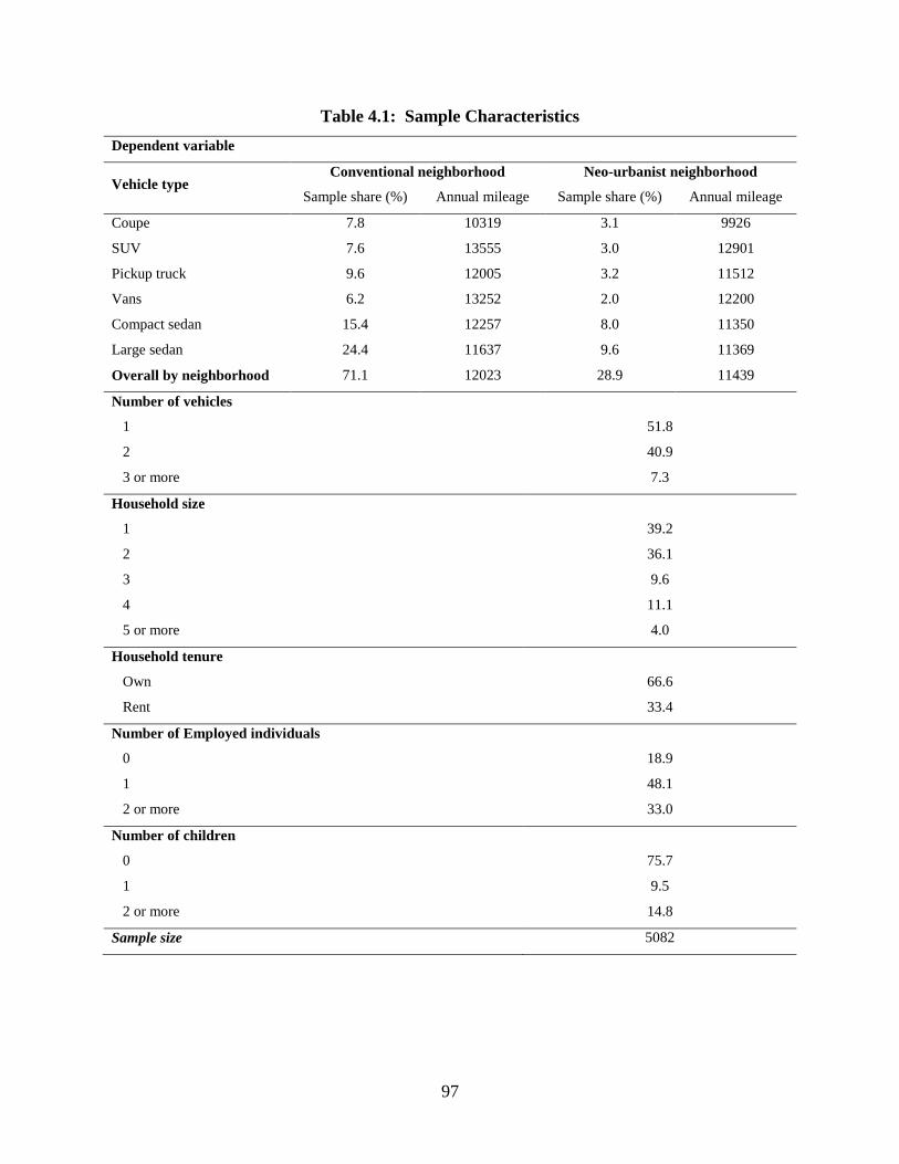
97
Table 4.1: Sample Characteristics
Dependent variable
Vehicle type Conventional neighborhood Neo-urbanist neighborhood
Sample share (%) Annual mileage Sample share (%) Annual mileage
Coupe 7.8 10319 3.1 9926
SUV 7.6 13555 3.0 12901
Pickup truck 9.6 12005 3.2 11512
Vans 6.2 13252 2.0 12200
Compact sedan 15.4 12257 8.0 11350
Large sedan 24.4 11637 9.6 11369
Overall by neighborhood 71.1 12023 28.9 11439
Number of vehicles
1 51.8
2 40.9
3 or more 7.3
Household size
1 39.2
2 36.1
3 9.6
4 11.1
5 or more 4.0
Household tenure
Own 66.6
Rent 33.4
Number of Employed individuals
0 18.9
1 48.1
2 or more 33.0
Number of children
0 75.7
1 9.5
2 or more 14.8
Sample size 5082
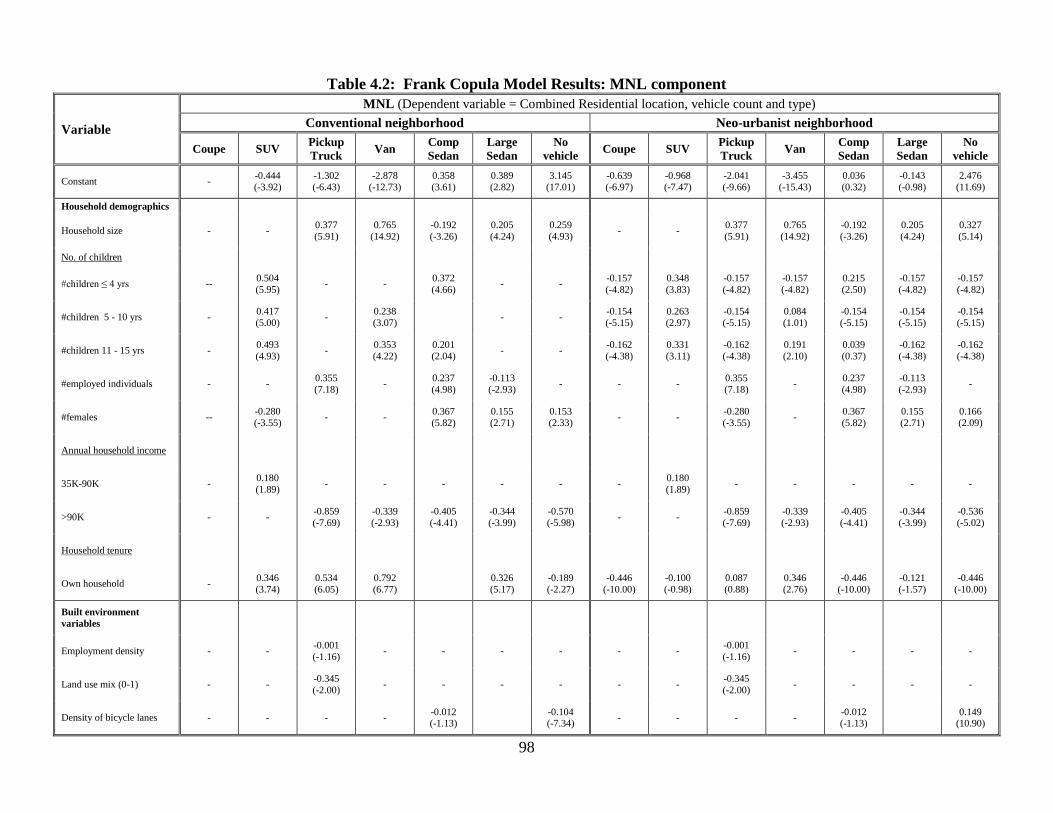
98
Table 4.2: Frank Copula Model Results: MNL component
Variable
MNL (Dependent variable = Combined Residential location, vehicle count and type)
Conventional neighborhood Neo-urbanist neighborhood
Coupe SUV Pickup
Truck Van
Comp
Sedan
Large
Sedan
No
vehicle Coupe SUV
Pickup
Truck Van
Comp
Sedan
Large
Sedan
No
vehicle
Constant - -0.444
(-3.92)
-1.302
(-6.43)
-2.878
(-12.73)
0.358
(3.61)
0.389
(2.82)
3.145
(17.01)
-0.639
(-6.97)
-0.968
(-7.47)
-2.041
(-9.66)
-3.455
(-15.43)
0.036
(0.32)
-0.143
(-0.98)
2.476
(11.69)
Household demographics
Household size - - 0.377
(5.91)
0.765
(14.92)
-0.192
(-3.26)
0.205
(4.24)
0.259
(4.93) - -
0.377
(5.91)
0.765
(14.92)
-0.192
(-3.26)
0.205
(4.24)
0.327
(5.14)
No. of children
#children ≤ 4 yrs -- 0.504
(5.95) - -
0.372
(4.66) - -
-0.157
(-4.82)
0.348
(3.83)
-0.157
(-4.82)
-0.157
(-4.82)
0.215
(2.50)
-0.157
(-4.82)
-0.157
(-4.82)
#children 5 - 10 yrs - 0.417
(5.00) -
0.238
(3.07) - -
-0.154
(-5.15)
0.263
(2.97)
-0.154
(-5.15)
0.084
(1.01)
-0.154
(-5.15)
-0.154
(-5.15)
-0.154
(-5.15)
#children 11 - 15 yrs - 0.493
(4.93) -
0.353
(4.22)
0.201
(2.04) - -
-0.162
(-4.38)
0.331
(3.11)
-0.162
(-4.38)
0.191
(2.10)
0.039
(0.37)
-0.162
(-4.38)
-0.162
(-4.38)
#employed individuals - - 0.355
(7.18) -
0.237
(4.98)
-0.113
(-2.93) - - -
0.355
(7.18) -
0.237
(4.98)
-0.113
(-2.93) -
#females -- -0.280
(-3.55) - -
0.367
(5.82)
0.155
(2.71)
0.153
(2.33) - -
-0.280
(-3.55) -
0.367
(5.82)
0.155
(2.71)
0.166
(2.09)
Annual household income
35K-90K - 0.180
(1.89) - - - - - -
0.180
(1.89) - - - - -
>90K - - -0.859
(-7.69)
-0.339
(-2.93)
-0.405
(-4.41)
-0.344
(-3.99)
-0.570
(-5.98) - -
-0.859
(-7.69)
-0.339
(-2.93)
-0.405
(-4.41)
-0.344
(-3.99)
-0.536
(-5.02)
Household tenure
Own household - 0.346
(3.74)
0.534
(6.05)
0.792
(6.77)
0.326
(5.17)
-0.189
(-2.27)
-0.446
(-10.00)
-0.100
(-0.98)
0.087
(0.88)
0.346
(2.76)
-0.446
(-10.00)
-0.121
(-1.57)
-0.446
(-10.00)
Built environment
variables
Employment density - - -0.001
(-1.16) - - - - - -
-0.001
(-1.16) - - - -
Land use mix (0-1) - - -0.345
(-2.00) - - - - - -
-0.345
(-2.00) - - - -
Density of bicycle lanes - - - - -0.012 (-1.13)
-0.104 (-7.34)
- - - - -0.012 (-1.13)
0.149
(10.90)
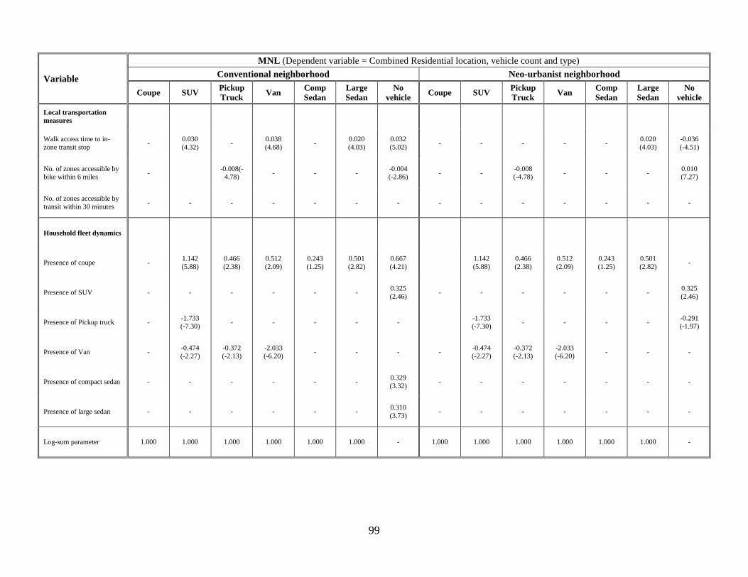
99
Variable
MNL (Dependent variable = Combined Residential location, vehicle count and type)
Conventional neighborhood Neo-urbanist neighborhood
Coupe SUV Pickup
Truck Van
Comp
Sedan
Large
Sedan
No
vehicle Coupe SUV
Pickup
Truck Van
Comp
Sedan
Large
Sedan
No
vehicle
Local transportation
measures
Walk access time to in-
zone transit stop -
0.030
(4.32) -
0.038
(4.68) -
0.020
(4.03)
0.032
(5.02) - - - - -
0.020
(4.03)
-0.036
(-4.51)
No. of zones accessible by bike within 6 miles
- -0.008(-
4.78) - - -
-0.004 (-2.86)
- - -0.008 (-4.78)
- - - 0.010 (7.27)
No. of zones accessible by
transit within 30 minutes - - - - - - - - - - - - - -
Household fleet dynamics
Presence of coupe - 1.142
(5.88)
0.466
(2.38)
0.512
(2.09)
0.243
(1.25)
0.501
(2.82)
0.667
(4.21)
1.142
(5.88)
0.466
(2.38)
0.512
(2.09)
0.243
(1.25)
0.501
(2.82) -
Presence of SUV - - - - - - 0.325
(2.46) - - - - - -
0.325
(2.46)
Presence of Pickup truck - -1.733
(-7.30) - - - - -
-1.733
(-7.30) - - - -
-0.291
(-1.97)
Presence of Van - -0.474
(-2.27)
-0.372
(-2.13)
-2.033
(-6.20) - - - -
-0.474
(-2.27)
-0.372
(-2.13)
-2.033
(-6.20) - - -
Presence of compact sedan - - - - - - 0.329
(3.32) - - - - - - -
Presence of large sedan - - - - - - 0.310
(3.73) - - - - - - -
Log-sum parameter 1.000 1.000 1.000 1.000 1.000 1.000 - 1.000 1.000 1.000 1.000 1.000 1.000 -
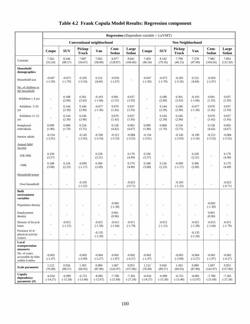
100
Table 4.2 Frank Copula Model Results: Regression component
Regression (Dependent variable = LnVMT)
Conventional neighborhood Neo Neighborhood
Coupe SUV Pickup
Truck Van
Com-
Sedan
Large
Sedan Coupe SUV
Pickup
Truck Van
Com-
Sedan
Large
Sedan
Constant 7.562
(53.24)
8.246
(80.57)
7.897
(54.67)
7.692
(58.89)
8.077
(128.87)
8.041
(160.66)
7.459
(46.54)
8.142
(79.16)
7.798
(46.13)
7.578
(47.09)
7.985
(104.56)
7.893
(131.50)
Household
demographics
Household size -0.047
(-1.50)
-0.073
(-1.70)
-0.205
(-3.16)
0.152
(4.64)
-0.059
(-1.67) -
-0.047
(-1.50)
-0.073
(-1.70)
-0.205
(-3.16)
0.152
(4.64)
-0.059
(-1.67) -
No. of children in
the household
#children ≤ 4 yrs - 0.188
(2.69)
0.301
(2.63)
-0.103
(-1.66)
0.091
(1.55)
0.037
(1.93) -
0.188
(2.69)
0.301
(2.63)
-0.103
(-1.66)
0.091
(1.55)
0.037
(1.93)
#children 5-10
yrs -
0.144
(2.39)
0.246
(2.90)
-0.077
(-1.36)
0.070
(1.42)
0.037
(1.93) -
0.144
(2.39)
0.246
(2.90)
-0.077
(-1.36)
0.070
(1.42)
0.037
(1.93)
#children 11-15
yrs -
0.144
(2.39)
0.246
(2.90) -
0.070
(1.42)
0.037
(1.93) -
0.144
(2.39)
0.246
(2.90) -
0.070
(1.42)
0.037
(1.93)
#employed
individuals
0.090
(1.80)
0.068
(1.70)
0.234
(3.75) -
0.158
(4.42)
0.093
(4.67)
0.090
(1.80)
0.068
(1.70)
0.234
(3.75) -
0.158
(4.42)
0.093
(4.67)
#senior adults -0.154
(-2.01) -
-0.145
(-2.03)
-0.190
(-3.16)
-0.212
(-5.53)
-0.084
(-3.55)
-0.154
(-2.01)
-0.145
(-2.03)
-0.190
(-3.16)
-0.212
(-5.53)
-0.084
(-3.55)
Annual hhld
income
35K-90K 0.330
(3.27) - -
0.228
(2.31) -
0.179
(4.49)
0.330
(3.27) - -
0.228
(2.31) -
0.179
(4.49)
>90K 0.348
(3.08)
0.126
(2.23)
-0.095
(-1.17)
0.306
(2.69) -
0.179
(4.49)
0.348
(3.08)
0.126
(2.23)
-0.095
(-1.17)
0.306
(2.69) -
0.179
(4.49)
Household tenure
Own household - - -0.105
(-1.22) - -
-0.023
(-0.71) - -
-0.105
(-1.22) - -
-0.023
(-0.71)
Built
environment
variables
Population density - - - - -0.002
(-1.39) - - - - -
-0.002
(-1.39) -
Employment
density - - - -
0.001
(0.90) - - - - -
0.001
(0.90) -
Density of bicycle
lanes -
-0.012
(-1.15) -
-0.021
(-1.58)
-0.012
(-1.64)
-0.011
(-1.79)
-0.012
(-1.15)
-0.021
(-1.58)
-0.012
(-1.64)
-0.011
(-1.79)
Presence of 4+
physical activity
centers
- - - -0.135
(-1.26) - - - - -
-0.135
(-1.26) - -
Local
transportation
measures
No. of zones
accessible by bike
within 6 miles
-0.002
(-1.47) -
-0.003
(-2.09)
-0.004
(-3.27)
-0.001
(-1.87)
-0.002
(-4.27)
-0.002
(-1.47) -
-0.003
(-2.09)
-0.004
(-3.27)
-0.001
(-1.87)
-0.002
(-4.27)
Scale parameter 1.122
(76.99)
0.926
(89.57)
1.303
(60.93)
0.989
(87.89)
1.007
(142.97)
0.953
(157.86)
1.122
(76.99)
0.926
(89.57)
1.303
(60.93)
0.989
(87.89)
1.007
(142.97)
0.953
(157.86)
Copula
dependency
parameter (θ)
-6.034 (-14.27)
-6.999 (-15.20)
-6.723 (-13.40)
-8.085 (-12.07)
-7.780 (-21.69)
-7.365 (-27.24)
-6.034 (-14.27)
-6.999 (-15.20)
-6.723 (-13.40)
-8.085 (-12.07)
-7.780 (-21.69)
-7.365 (-27.24)
101
CHAPTER 5 ACTIVITY PARTICIPATION DECISIONS
5.1 Introduction and motivation
Emerging policy issues of interest, including concerns regarding global climate change
and the desire to better understand how pricing policies and technological innovations
impact travel demand, enhanced understanding of activity-travel behavior dimensions
garnered over decades of behavioral research, and advances in microsimulation-based
computational approaches have all contributed to a new era in travel demand modeling
and forecasting (Pendyala et al, 2005; Pinjari et al, 2006). This era is characterized by an
increasing shift towards activity-based travel demand modeling approaches that explicitly
recognize that travel is undertaken to fulfill activity needs and desires dispersed in space
and time (Meloni et al, 2004). The move towards microsimulation-based approaches
facilitates the disaggregate representation of behavioral agents and their interactions,
while simultaneously incorporating the ability to analyze policy impacts and address
equity concerns at the level of the individual traveler or any sub-market segment of
interest (Miller and Roorda, 2003).
Within the scope of this chapter, it is not possible to thoroughly review the
developments in activity-based models over the past decade and the gradual
implementation of tour-based models in practice in several urban areas in the United
States and other parts of the world (see Chapter 1 for review of operational activity-based
models). Regardless of the specific model design adopted, it is found that activity and
tour-based model systems universally strive to mimic and replicate activity-travel choice
processes of individuals. These choice processes include such dimensions as activity
type choice, time of day choice, trip chaining or linking choice, joint versus solo activity
engagement choice, destination choice, mode choice, activity sequencing decisions, and
activity time allocation (duration) decisions. Many of these choice processes are discrete
in nature (e.g., activity type choice, time of day period choice, mode and destination
choices), while a few may be more continuous in nature (e.g., activity duration). Given
the large number of choices that are involved in the behavioral process, many models,
102
particularly the tour-based models in practice, resort to the adoption of deeply nested
logit models (Ben-Akiva and Lerman, 1985) where one choice process is nested within
another choice process and so on, forming a long chain of inter-connected nests to
complete the representation of the behavioral process (Bowman, 1995; Bowman and
Bradley, 2006; PB Consult, 2005). As it is virtually impossible to estimate such long
chains of nested logit models simultaneously (i.e., in one single step), components of the
nested logit model are usually estimated one step (or maybe two steps) at a time and the
logsum from one level is carried up to the next higher level, resulting in a sequential
estimation and model application approach. Although there are other behavioral model
systems that attempt to move away from such deeply nested logit specifications, such as
those based on computational process modeling and heuristic approaches (Arentze and
Timmermans, 2005), the fact remains that most activity-based model systems break down
the behavioral decision process so that one is modeling only one or two choice processes
at any step in the model system.
5.1.1 Joint model systems
Although a sequential treatment of choice mechanisms is convenient from a
practical model estimation and application standpoint, it is unclear whether such model
systems truly replicate behavioral processes. While tour-based and activity-based models
in practice can be lauded for their ability to model activity engagement patterns, consider
interactions among activities and trips, and microsimulate activity-travel patterns at the
level of the individual traveler, the issue arises as to whether these model systems can be
challenged and questioned from a behavioral standpoint not unlike the traditional four-
step travel modeling process. The four-step travel modeling process has been
consistently criticized for its sequential nature of treatment of the travel demand process.
To what extent activity and tour-based models in practice overcome this issue is
potentially open to debate, although there is no question that even limited information
maximum likelihood (LIML) specifications of deeply nested logit models allow one to
103
model correlated choice processes better than was done in the four-step travel modeling
process.
While it is arguably true that people have limited cognitive abilities and therefore
exercise choices in a limited, sequential way, there is considerable evidence that many
choices are made jointly or simultaneously and that there are significant unobserved
factors that simultaneously impact multiple choice dimensions (see, for example, Pinjari
and Bhat, 2009a). In fact, one could argue that the limited information sequential model
specifications have been adopted in the activity-based modeling realm because of the
estimation challenges and computational complexity associated with specifying,
identifying, and estimating simultaneous equations model systems that represent joint
choice processes in which individuals and households are making a “package” of
activity-travel choices as a “bundle”. In other words, it is conceivable that individual
agents are making choices regarding the type of activity to pursue, the mode and
destination, and the time allocation to the activity in one swoop, thus motivating the
adoption of a “joint” choice model specification in which unobserved factors unknown to
the analyst may be simultaneously impacting multiple dimensions of interest (Jara-Diaz
et al, 2007).
5.1.2 Current research effort
The growing interest in the ability to model multiple choice dimensions simultaneously,
where the endogeneity of many choice variables is explicitly recognized in the activity-
travel behavior modeling arena, motivates this research effort. Specifically, this chapter
presents a joint model system of five choice dimensions:
Activity type choice
Activity time of day choice (treated as discrete time intervals)
Mode choice
Destination choice
Activity duration (continuous choice dimension)
104
These five choice dimensions are of critical interest to any activity-based model
system regardless of the model design that might be adopted. Thus, this study aims to
specify and estimate a comprehensive econometric model system that jointly models
these five choice dimensions in a holistic unifying utility-maximization framework. The
model system explicitly includes consideration of built environment attributes including
level of service variables and spatial land use characteristics to capture the potential
impacts of such variables on the activity generation process, a key area that warrants
additional research. Such a model specification provides the ability to examine induced
and suppressed demand effects in response to changes in system capacity and level of
service.
The modeling methodology adopted in this study builds on previous work by the
authors and constitutes a joint multiple discrete continuous extreme value model and
multinomial logit model system (Bhat 2005, Bhat et al., 2006, Bhat 2008). The multiple
discrete continuous extreme value (MDCEV) model component is used to jointly analyze
activity type choice, activity time of day choice, mode choice, and activity duration.
Specifically, the MDCEV model is used to represent activity participation (discrete
choice) and time use (continuous choice) for different types of activities at different time
periods of the day by different travel modes. The activity location choice is modeled
using a multinomial logit (MNL) model nested within the MDCEV framework. The
model system is estimated for a survey sample drawn from the 2000 San Francisco Bay
Area Travel Survey (BATS), a comprehensive database that includes detailed household
and personal socio-economic, demographic, and activity-travel information together with
a host of secondary transportation level-of-service and land use variables.
The next section presents the modeling methodology in detail. This is followed
by a description of the dataset and survey sample. The fourth and fifth sections present
model estimation and policy simulation results, while the sixth and final section offers
concluding remarks.
105
5.2 Modeling methodology
This section presents the modeling methodology for the joint MDCEV-MNL model
structure. First, the utility structure is presented, second, the econometric model
specification is presented, and finally the procedure for sampling of location choice
alternatives is discussed. An intuitive behavioral interpretation of the model structure is
offered as well.
5.2.1 Utility Structure
Consider the following utility specification for the integrated analysis of individuals‟
activity time-use, timing, mode choice, and location choice decisions:
62
21 1 2 2
32
( ) ln ln 1 ln 1ptm
ptm ptm
ptm ptm
xxU x
x (5.1)
In the above equation, the first term 11 ln x corresponds to the utility contribution
of the total daily time invested 1( )x in all maintenance activities, and the second term
corresponds to the utility contribution of the total daily time invested 2( )x in all in-home
(IH) discretionary activities. The next set of terms correspond to the utility contribution
due to the time investment ( )ptmx in out-of-home (OH) discretionary activity episode
types (indexed by ptm), with each activity episode type defined by its purpose (p), timing
(t), and mode of travel (m). In the current empirical context considered in this chapter,
there are five OH discretionary activity purposes (volunteering, socializing, recreation,
meals, and shopping), six time periods (3am-7am or early morning, 7am-9am or morning,
9am-12noon or late morning, 12noon-4pm or afternoon, 4pm-7pm or evening, and 7pm-
3am or night), and two modes of travel (auto, and non-auto), yielding 60 different types
of OH discretionary activity episodes (or ptm combinations). Thus, there are a total of 62
MDCEV choice alternatives in that one or more of these alternatives may be chosen by
106
an individual through the course of a day.10
For each of these alternatives, the terms (
1 2, ,and ptm ) are the baseline utility parameters that control the discrete choice of the
alternative. For all alternatives except the first alternative, the terms (2 and ptm )
allow for corner solutions (i.e., the possibility of not choosing the alternative) as well as
satiation effects (i.e., diminishing marginal utility with increasing time investment).11
There is no term corresponding to the first alternative (maintenance activity) as it is
always chosen by all individuals.
Finally, let each of the 60 OH discretionary activity episode types (ptm) be
defined (by its purpose-timing-mode (ptm) combination) such that an individual
participates in no more than one episode of that type in a day. Consequently, if an
individual chooses to undertake an activity episode type (ptm), it has to be at only one of
the several destination alternatives (l) available to her/him.
Let the index for the activity destination (or location) be l, and let ptmN be the set
of destinations available for an activity episode type (ptm). Further, for each activity
episode type (ptm), let ptm be defined as follows (Bhat et al., 2006):
exp ,ptm
ptm lptm lptm
l N
W
(5.2)
where, lptmW is the utility perceived by the individual for undertaking the OH discretionary
activity episode of purpose p, during time period t, by traveling on mode m to location l,
10 Without loss of generality, all individuals can be assumed to participate in maintenance activities. On the
other hand, an individual can participate in none, or one, or more of IH discretionary and 5 OH
discretionary activity purposes (p) identified above. If (s)he chooses to participate in OH discretionary
activities, (s)he can do so during one or more of the 6 time periods (t), and access the activities using one or
more of the 2 travel modes (m). Thus, there is multiple discreteness in the choices across the activity
purpose, activity timing, and travel mode dimensions. 11
To distinguish the satiation along OH discretionary activity purpose, activity timing, and travel mode
dimensions (and to facilitate estimation), ptm (ptm = 3,4,…,62) is parameterized as ptm p t m ,
where p , t , m are the estimated dimension-specific satiation parameters.
107
and lptm is a dummy variable taking a value of 1 if the l
th location is chosen for that
activity episode such that ( ) 1ptm
lptml N
(i.e., only one location is chosen).
With the above definition of ptm and other terms described earlier, the individual
is assumed to maximize the utility function ( )U x in Equation (5.1) subject to
1 2 ;ptm
ptm
x x x X 1 0,x 2 0,x 0 3,4,...62.ptmx ptm Since the individual
maximizes ( )U x and can choose only one location for each activity episode ptm type, the
functional form of ( )U x implies that the individual will consider the location that
provides the maximum utility for each activity episode ptm type in the process of
maximizing ( )U x (see Bhat et al., 2008). That is, maxptm
ptm
lptm lptm lptml N
l N
W W
, or
exp maxptm
ptm lptml N
W
Thus, the individual‟s utility maximizing problem can be written
as:
21 1 2 2
2
( ) ln ln 1 exp max ln 1ptm
ptm
ptm lptml N
ptm ptm
xxU x W
x (5.3)
subject to 1 2 ;ptm
ptm
x x x X 1 0,x 2 0,x 0 .ptmx ptm
The analyst can solve for the optimal values of 1 2, ,and ptmx x x by forming the
Lagrangian and applying the Kuhn-Tucker (KT) conditions. Specifically, the following
KT conditions can be formed (see Bhat, 2008):
0 212 xifHH (5.4)
2 1 2 0H H if x
1 0ptm ptmH H if x
1 0ptm ptmH H if x
where,
108
1 1 1
22 2
2
ln( ) ln( ),
ln( ) ln 1 , and
max ln 1ptm
ptm
ptm lptml N
ptm
H x
xH
xH W
5.2.2 Econometric Structure
To complete the model specification, let 1 1 1exp( )z and
2 2 2exp( )z ,
where 1z and 2z are the observed baseline utility components of maintenance and IH
discretionary activities, respectively, and 1 and 2 are the corresponding unobserved
components assumed to be independent and identically Gumbel distributed. Further, to
define ptm , we expand
lptmW as:
lptm ptm lptm lptmW z w (5.5)
where, ptmz is the observed baseline utility corresponding to the activity purpose,
timing, and mode of the OH discretionary activity episode ptm, lptmw is the observed
utility corresponding to the potential location l for the activity episode, and lptm is the
unobserved utility component associated with the location l of activity episode ptm.
Similar to 1 and 2 , the lptm terms are assumed to be independent and identically
distributed (across different activity episode ptm types) Gumbel terms. Within each
activity episode ptm type, however, all the error terms may share common unobserved
attributes (specific to the activity episode ptm type) generating correlations among the
lptm terms across all potential locations for the activity episode. Thus, for each activity
episode ptm type, the following distribution of error terms may be used:
1 2
/ / /
1 2( , ,..., ) exp ...ptm
ptm ptm ptm ptm Lptm ptm
ptm ptm LptmF e e e
(5.6)
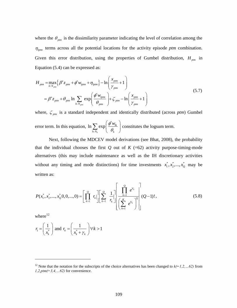
109
where the ptm is the dissimilarity parameter indicating the level of correlation among the
lptm terms across all the potential locations for the activity episode ptm combination.
Given this error distribution, using the properties of Gumbel distribution, ptmH in
Equation (5.4) can be expressed as:
max ln 1
ln exp ln 1
ptm
ptm
ptm
ptm ptm lptm lptml N
ptm
lptm ptm
ptm ptm ptm
l N ptm ptm
xH z w
w xz
(5.7)
where, ptm is a standard independent and identically distributed (across ptm) Gumbel
error term. In this equation, ln expk
lk
l N k
w
constitutes the logsum term.
Next, following the MDCEV model derivations (see Bhat, 2008), the probability
that the individual chooses the first Q out of K (=62) activity purpose-timing-mode
alternatives (this may include maintenance as well as the IH discretionary activities
without any timing and mode distinctions) for time investments * * *
1 2, ,..., Qx x x may be
written as:
* * * 11 2
11
1
1( , ,..., 0,0,...,0) ( 1)!
k
h
QV
Q Q
kQ k Q
Kkk k V
h
e
P x x x r Qr
e
, (5.8)
where12
1 * *
1 1and 1k
k k k
r r kx x
12 Note that the notation for the subscripts of the choice alternatives has been changed to k(=1,2,…62) from
1,2,ptm(=3,4,…62) for convenience.
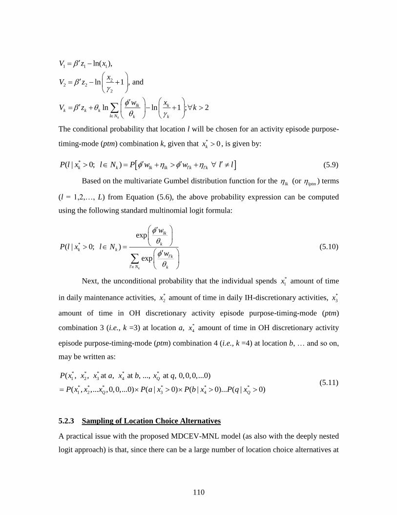
110
1 1 1
22 2
2
ln( ),
ln 1 , and
ln ln 1 ; 2k
lk kk k k
l N k k
V z x
xV z
w xV z k
The conditional probability that location l will be chosen for an activity episode purpose-
timing-mode (ptm) combination k, given that * 0kx , is given by:
*( | 0; ) k k lk lk l k l kP l x l N P w w l l (5.9)
Based on the multivariate Gumbel distribution function for the lk (or lptm ) terms
(l = 1,2,…, L) from Equation (5.6), the above probability expression can be computed
using the following standard multinomial logit formula:
*
exp
( | 0; )
expk
lk
k
k k
l k
l N k
w
P l x l Nw
(5.10)
Next, the unconditional probability that the individual spends *
1x amount of time
in daily maintenance activities, *
2x amount of time in daily IH-discretionary activities, *
3x
amount of time in OH discretionary activity episode purpose-timing-mode (ptm)
combination 3 (i.e., k =3) at location a, *
4x amount of time in OH discretionary activity
episode purpose-timing-mode (ptm) combination 4 (i.e., k =4) at location b, … and so on,
may be written as:
* * * * *
1 2 3 4
* * * * * *
1 2 3 4
( , , at , at , ..., at , 0,0,0,...0)
( , ,... ,0,0,...0) ( | 0) ( | 0)... ( | 0)
Q
Q Q
P x x x a x b x q
P x x x P a x P b x P q x (5.11)
5.2.3 Sampling of Location Choice Alternatives
A practical issue with the proposed MDCEV-MNL model (as also with the deeply nested
logit approach) is that, since there can be a large number of location choice alternatives at
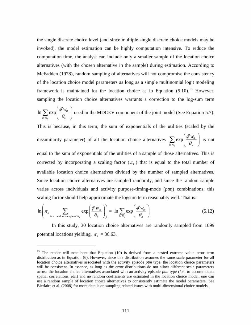
111
the single discrete choice level (and since multiple single discrete choice models may be
invoked), the model estimation can be highly computation intensive. To reduce the
computation time, the analyst can include only a smaller sample of the location choice
alternatives (with the chosen alternative in the sample) during estimation. According to
McFadden (1978), random sampling of alternatives will not compromise the consistency
of the location choice model parameters as long as a simple multinomial logit modeling
framework is maintained for the location choice as in Equation (5.10).13
However,
sampling the location choice alternatives warrants a correction to the log-sum term
ln expk
lk
l N k
w
used in the MDCEV component of the joint model (See Equation 5.7).
This is because, in this term, the sum of exponentials of the utilities (scaled by the
dissimilarity parameter) of all the location choice alternatives expk
lk
l N k
w
is not
equal to the sum of exponentials of the utilities of a sample of those alternatives. This is
corrected by incorporating a scaling factor ( k ) that is equal to the total number of
available location choice alternatives divided by the number of sampled alternatives.
Since location choice alternatives are sampled randomly, and since the random sample
varies across individuals and activity purpose-timing-mode (ptm) combinations, this
scaling factor should help approximate the logsum term reasonably well. That is:
a random sample of
ln exp ln expk k
lk lkk
l N l Nk k
w w
(5.12)
In this study, 30 location choice alternatives are randomly sampled from 1099
potential locations yielding, k = 36.63.
13 The reader will note here that Equation (10) is derived from a nested extreme value error term
distribution as in Equation (6). However, since this distribution assumes the same scale parameter for all
location choice alternatives associated with the activity episode ptm type, the location choice parameters
will be consistent. In essence, as long as the error distributions do not allow different scale parameters
across the location choice alternatives associated with an activity episode ptm type (i.e., to accommodate
spatial correlations, etc.) and no random coefficients are estimated in the location choice model, one can
use a random sample of location choice alternatives to consistently estimate the model parameters. See
Bierlaire et al. (2008) for more details on sampling related issues with multi-dimensional choice models.
112
5.2.4 An Intuitive Behavioral Interpretation
The probability expression in Equation (5.11) is a combination of MDCEV and single
discrete choice probabilities. Specifically, for each OH discretionary activity episode
purpose-timing-mode (ptm) combination chosen by an individual, a single discrete choice
model of location choice is invoked. The parameters and k appear in both the
MDCEV probability expression (Equation 5.8) as well as the standard discrete choice
probability expression for the choice of activity location (Equation 5.10) to create
jointness between the multiple discrete-continuous and single discrete choices. Further,
the logsum term (see Equation 5.7) appearing in the MDCEV probability expression
carries the accessibility of destinations (or potential locations) from the single discrete
location choice model to the MDCEV model of time investment by activity purpose,
timing, and travel mode. Thus, Equation (5.11) represents a unified and comprehensive
model of activity-travel program generation that incorporates the influence of
accessibility measures on activity time-use, timing, and mode choices.
The proposed two-level MDCEV-MNL model is an attractive alternative to the
deeply nested logit modeling approach available in the literature, where accessibility
measures have to propagate up to the activity generation level through multiple levels of
a deeply nested logit model. Further, the MDCEV-MNL model provides a seamless way
of incorporating time-use (and the impact of accessibility on time-use) into the
framework. Specifically, the modeling framework explicitly accommodates the concept
that individual‟s activity time-use (i.e., time allocation) decisions are important and
influential components of their activity-travel decision-making (Bhat and Koppelman,
1999). On the other hand, the deeply nested logit approach does not explicitly incorporate
activity time-allocation choices into the analysis framework in a straight forward manner.
Another appealing feature is that the model recognizes the simultaneity of the activity
time-use, timing, mode choice, and location choice decisions within a unified utility
maximization framework.
113
5.3 Data Description
The data set used in this chapter is derived from the 2000 San Francisco Bay Area Travel
Survey (BATS), designed and administered by MORPACE International Inc. for the Bay
Area Metropolitan Transportation Commission (MTC). The data includes information
on: (1) Individual and household socio-demographics for over 15,000 households in the
Bay Area, and (2) All activity episodes (including activity type, start and end times of the
activity, geo-referenced location of activity participation, and mode of travel to the
activity) undertaken by the individuals in all surveyed households for a two-day period.
The travel survey records were augmented extensively with several secondary
data items, including land-use characteristics, transportation network level-of-service
data, and Census population and housing data. In addition, geo-referenced data on
businesses, bicycle facilities, highways and local roads were used to derive spatial
variables characterizing the activity-travel environment (ATE) in and around the
household locations of the individuals in the data set. Details regarding the data
preparation and augmentation processes can be found in Guo and Bhat (2004) and Pinjari
et al., (2009).
As mentioned in the previous section, the activity choice dimensions modeled in
this research effort include activity type choice, activity time of day choice, travel mode
choice, activity location (destination) choice, and activity time use allocation (duration).
The MDCEV model component alternatives are formed as combinations of activity type,
time of day, and travel mode while the duration of each activity episode constitutes the
continuous dependent variable. Finally, the MNL module accommodates the activity
location or destination choice. There are: (a) a maintenance activity type, (b) an in-home
discretionary activity type, and (c) five out-of-home discretionary activity types, six time
periods, and two travel modes, yielding a total of 62 possible MDCEV choice alternatives
(2 + 5x6x2 = 62). It is to be noted that the activity timing and travel mode analysis is
limited to the five out-of-home discretionary activity types.
114
In order to control for fundamental differences between workers and non-workers
in their activity engagement patterns and choice processes, and in the interest of brevity,
the analysis in this chapter was restricted to the sample of 5,360 non-working individuals
aged 16 years or above. Descriptive statistics for this sample of individuals are presented
in Table 5.1. All 5,360 individuals participate in in-home maintenance for an average
duration of nearly 11 hours. Forty percent engage in in-home discretionary activities for
an average duration of about 5.5 hours. Note that the average durations are computed
over those who actually participate in the activity type. A little over one-half of the
sample participated in OH discretionary activities, for an average duration of about 2.5
hours. It is found that the automobile mode is the preferred and dominant mode of travel
accounting for nearly 90 percent of all out-of-home discretionary activity engagement.
Non-maintenance shopping shows a relatively high participation rate, but lower time
allocation (regardless of mode), while activities such as meals, socializing, and recreation
show lower participation rates but higher time allocation. Across the top of the table (in
the grey shaded row), it is seen that only a very small percent of individuals participate in
OH discretionary activities in the early morning, and the percentage steadily rises into the
afternoon, and then shows a decline towards the night hours. Activities undertaken in the
morning and early morning, however, show the longest average durations relative to
those in the afternoon and evening, potentially indicating the effect of time constraints
that might get tighter towards the latter half of the day. Overall, this table shows the
interplay among the dimensions of activity-travel participation that merit a unified
approach towards modeling these behavioral characteristics.
5.4 Empirical analysis
5.4.1 Model specification and estimation
Model estimation was performed using Gauss code written specifically to estimate the
joint MDCEV-MNL model system. Although it would have been ideal to estimate a
separate destination choice model for each of the 60 OH discretionary activity purpose-
timing-mode (ptm) combination categories, for this initial effort, a single MNL location
115
choice model was estimated for all discretionary activity ptm categories. However,
extending the estimation process to incorporate 60 MNL models of destination choice is
straightforward by specifying dimension-specific model coefficients; the model
specification here is one in which all destination choice model coefficients are restricted
to be identical across all activity purpose categories, timing categories, and mode
categories. A variety of variables were included in the model specification including
household and personal socio-economic and demographic variables, contextual variables
such as day of week and season of the year, and a host of spatial variables characterizing
the activity-travel environment (ATE) around the household locations, not to mention
several transportation network level of service variables. The spatial ATE variables
included density measures, activity opportunity and accessibility measures, and
population and housing data for the neighborhood (traffic analysis zone). The ATE
measures were considered at the level of the traffic analysis zone and at finer spatial
resolutions, including within 0.25 mile, 1 mile, and 5 mile radii buffers of the household
location (see Guo and Bhat, 2004 and Pinjari et al, 2009 for complete details).
5.4.2 Model assessment
In the current research effort, a comparison was made between the joint MDCEV-MNL
model that integrates destination choice with activity choices and an independent
MDCEV-MNL model that does not incorporate the log-sum parameters in the MDCEV
component. The goodness of fit of the two models were compared using the Bayesian
Information Criterion (BIC), which is given by the expression
2 ln( ) ln( )L number of parameters Q , where ln( )L is the log-likelihood value at
convergence and Q is the number of observations. The model that results in the lower
BIC value is the preferred model. The BIC value for the MDCEV-MNL model (with 103
model parameters) is,150514.2 which is substantially lower than that for the independent
MDCEV-MNL model (152334.2 with 102 model parameters). Thus, the BIC clearly
favors the MDCEV-MNL model of integrated activity choices and destination choice.
116
5.4.3 Estimation results
The discussion in this chapter is limited to the results of the joint MDCEV-MNL model.
The MDCEV component is specified (and the results are presented) in such a way that
the effect of each variable is first identified separately along the activity purpose, activity
timing and travel mode dimensions. Subsequently, any interaction effects of the variable
over and above the uni-dimensional effects are identified. A blank entry corresponding to
the effect of a variable indicates no significant effect of the variable on the integrated
choice process. Further, the effects of variables on the baseline utilities have been
constrained to be equal if coefficient equality could not be rejected based on statistical
tests. Finally, t-statistics are presented in parentheses. The final specification of the
MDCEV component of the model is presented in Table 5.2. In the interest of brevity, and
considering the large number of alternatives (62), tables showing estimates of baseline
preference constants and satiation parameters are not furnished here.
Overall, the model results show indications as expected. Larger household sizes
are associated with greater levels of participation in maintenance activities (in and out of
home), while single persons are more prone to out-of-home socializing and recreation in
the evening. The presence of very young kids motivates activity engagement in the
prime period of the day as opposed to early mornings and late nights, although those with
school age children are more restricted to pre- and post-school hours. The number of
working adults contributes negatively to activity engagement in the middle of the day,
presumably due to work constraints. Lower income individuals are more prone to in-
home discretionary activities, while higher income individuals are prone to undertake
out-of-home activities, consistent with expectations. Higher levels of car ownership
contribute negatively to in-home activity participation and non-auto mode use.
Females are more likely to engage in volunteering and maintenance activities,
particularly in the midday period, confirming the role of gender differences in activity
engagement. Younger individuals are likely to socialize in the evening and night, while
older individuals (65+ years) are more likely to volunteer and not undertake night
activities. Those who are licensed to drive have a greater propensity for out-of-home
117
activities, while the reverse is true for those physically disabled. Employed individuals
engage less in maintenance activities and in-home discretionary activities, even on days
that they do not work (this analysis was limited to non-working days for all 5,360
individuals, whether they are employed or not). Fridays are associated with greater out-
of-home discretionary activity participation, and night time activities. On rainy days, it is
less likely that individuals will eat out using non-auto modes. Population density
contributes positively to out-of-home meals, shopping by non-auto mode, possibly
because such areas are better served by transit and have better walk and bicycle access to
destinations. Overall, the findings are consistent with expectations and consistent with
those found earlier by Pinjari and Bhat (2009a).
The estimation results for the destination choice model are presented in Table 5.3.
The destination choice model component was estimated with 30 randomly sampled
choice alternatives for each location choice decision. The effects of transportation
network level of service, built environment, and demographic interaction terms were
represented in the final model specification. Auto travel times and costs decrease the
utility associated with choosing a destination for any activity type. The presence of
bicycle lanes, total employment, the size of the zone, and zonal household income
positively impact destination choice for discretionary activities while retain and service
employment, increasing fraction of land devoted to residential uses in the zone, and
accessibility to passive and natural recreation contribute negatively to destination choice
for the activity categories considered in this study. The long list of interaction terms
demonstrates how household and personal socio-economic and demographic
characteristics play a key role in influencing destination choice for discretionary activities
undertaken outside home. In the interest of brevity, a detailed explanation is not provided
here, but suffice to say that all of the interaction terms included in the model specification
are highly significant and indicate that household socio-economic and demographic
characteristics serve to moderate or enhance the likelihood of choosing a certain type of
destination for activity engagement. For example, females are more prone to choosing
destinations with high density of eat-out centers, as are older people and higher income
118
individuals. Those with kids and in larger households are less prone to choose zones with
high household density as destinations, presumably because they prefer more open space
and suburban locations to accommodate family activities.
The logsum parameters ( ptm ) estimated for each activity purpose, timing, and
travel mode combination were not statistically different from unity. In the final model
estimation, all logsum parameters were restricted equal to one. This implies the absence
of common unobserved factors across all location choice alternatives specific to an
activity type, timing, and mode combination. Note that this finding does not imply
independence between the MDCEV and MNL model components; rather the logsum
variables tie the two model components together, where as the logsum parameters
represent only the presence (or absence) of correlated unobserved factors across
destination choice alternatives for each activity type, timing, and mode combination
category.
5.5 Summary
This study aims to present a comprehensive unified model system of activity-travel
choices that is consistent with microeconomic utility maximization theory of behavior.
The activity-travel choice dimensions analyzed in this chapter include activity type
choice, time of day choice, mode choice, destination choice, and activity time allocation
or duration. All discrete choices, except for activity destination choice, and the
continuous choice dimension of activity duration are modeled simultaneously using the
multiple discrete continuous extreme value (MDCEV) model form while the destination
choice is modeled using a classic multinomial logit model (MNL) component. The
model components are tied together within a utility maximization-consistent framework
using logsum variables that reflect the accessibility of destinations for each activity type,
timing, and mode combination. Model estimation results and the policy simulation
analysis showed that the joint model system has merit, offers behaviorally intuitive
interpretation, and offers a goodness of fit statistically superior to that offered by an
independent model system that treats various choice dimensions separately and
119
sequentially. The model specifications included built environment and transportation
network level of service attributes demonstrating the impact of these variables on
activity-travel dimensions. The model system is presented for a non-worker sample
drawn from the 2000 San Francisco Bay Area Travel Survey (BATS). One of the key
empirical findings of this analysis is that the built environment and transportation
network level of service attributes of the destinations significantly impact activity time
use allocation, an aspect that is often overlooked in the literature.
The model form adopted in this study has key implications for activity-travel
demand model development. It appears that the findings reported here support the notion
that individuals make several activity-travel choices jointly as a “bundle”, calling for the
simultaneous modeling of various choice dimensions in a unifying framework. Activity-
travel model systems that purport to simulate the behavior of agents along the time axis
may benefit from the adoption of model forms that are able to simultaneously predict
multiple choice dimensions as a “bundle”. Ignoring to do so may yield erroneous policy
scenario predictions.
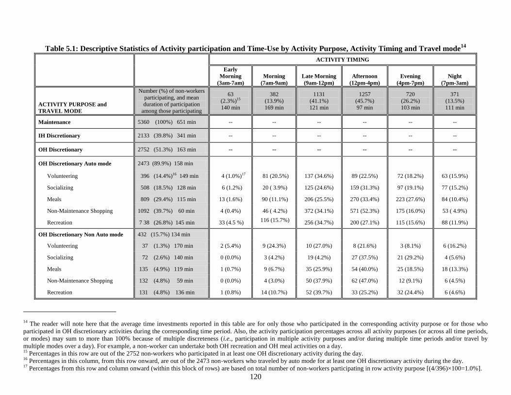
120
Table 5.1: Descriptive Statistics of Activity participation and Time-Use by Activity Purpose, Activity Timing and Travel mode14
ACTIVITY TIMING
Early
Morning
(3am-7am)
Morning
(7am-9am)
Late Morning
(9am-12pm)
Afternoon
(12pm-4pm)
Evening
(4pm-7pm)
Night
(7pm-3am)
ACTIVITY PURPOSE and
TRAVEL MODE
Number (%) of non-workers
participating, and mean
duration of participation
among those participating
63
(2.3%)15
140 min
382
(13.9%)
169 min
1131
(41.1%)
121 min
1257
(45.7%)
97 min
720
(26.2%)
103 min
371
(13.5%)
111 min
Maintenance 5360 (100%) 651 min -- -- -- -- -- --
IH Discretionary 2133 (39.8%) 341 min -- -- -- -- -- --
OH Discretionary 2752 (51.3%) 163 min -- -- -- -- -- --
OH Discretionary Auto mode 2473 (89.9%) 158 min
Volunteering 396 (14.4%)16 149 min 4 (1.0%)17 81 (20.5%) 137 (34.6%) 89 (22.5%) 72 (18.2%) 63 (15.9%)
Socializing 508 (18.5%) 128 min 6 (1.2%) 20 ( 3.9%) 125 (24.6%) 159 (31.3%) 97 (19.1%) 77 (15.2%)
Meals 809 (29.4%) 115 min 13 (1.6%) 90 (11.1%) 206 (25.5%) 270 (33.4%) 223 (27.6%) 84 (10.4%)
Non-Maintenance Shopping 1092 (39.7%) 60 min 4 (0.4%) 46 ( 4.2%) 372 (34.1%) 571 (52.3%) 175 (16.0%) 53 ( 4.9%)
Recreation 7 38 (26.8%) 145 min 33 (4.5 %) 116 (15.7%)
256 (34.7%) 200 (27.1%) 115 (15.6%) 88 (11.9%)
OH Discretionary Non Auto mode 432 (15.7%) 134 min
Volunteering 37 (1.3%) 170 min 2 (5.4%) 9 (24.3%) 10 (27.0%) 8 (21.6%) 3 (8.1%) 6 (16.2%)
Socializing 72 (2.6%) 140 min 0 (0.0%) 3 (4.2%) 19 (4.2%) 27 (37.5%) 21 (29.2%) 4 (5.6%)
Meals 135 (4.9%) 119 min 1 (0.7%) 9 (6.7%) 35 (25.9%) 54 (40.0%) 25 (18.5%) 18 (13.3%)
Non-Maintenance Shopping 132 (4.8%) 59 min 0 (0.0%) 4 (3.0%) 50 (37.9%) 62 (47.0%) 12 (9.1%) 6 (4.5%)
Recreation 131 (4.8%) 136 min 1 (0.8%) 14 (10.7%) 52 (39.7%) 33 (25.2%) 32 (24.4%) 6 (4.6%)
14 The reader will note here that the average time investments reported in this table are for only those who participated in the corresponding activity purpose or for those who
participated in OH discretionary activities during the corresponding time period. Also, the activity participation percentages across all activity purposes (or across all time periods,
or modes) may sum to more than 100% because of multiple discreteness (i.e., participation in multiple activity purposes and/or during multiple time periods and/or travel by
multiple modes over a day). For example, a non-worker can undertake both OH recreation and OH meal activities on a day. 15
Percentages in this row are out of the 2752 non-workers who participated in at least one OH discretionary activity during the day. 16
Percentages in this column, from this row onward, are out of the 2473 non-workers who traveled by auto mode for at least one OH discretionary activity during the day. 17
Percentages from this row and column onward (within this block of rows) are based on total number of non-workers participating in row activity purpose [(4/396)×100=1.0%].
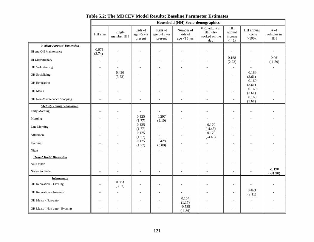
121
Table 5.2: The MDCEV Model Results: Baseline Parameter Estimates
Household (HH) Socio-demographics
HH size Single
member HH
Kids of
age <5 yrs
present
Kids of
age 5-15 yrs
present
Number of
kids of
age <15 yrs
# of adults in
HH who
worked on the
day
HH
annual
income
< 45k
HH annual
income
>100k
# of
vehicles in
HH
‘Activity Purpose’ Dimension
IH and OH Maintenance 0.071
(3.74) - - - - - - - -
IH Discretionary - - - - - - 0.168
(2.92) -
-0.061
(-1.89)
OH Volunteering - - - - - - - - -
OH Socializing - 0.420
(3.73) - - - - -
0.169
(3.61) -
OH Recreation - - - - - - - 0.169
(3.61) -
OH Meals - - - - - - - 0.169
(3.61) -
OH Non-Maintenance Shopping - - - - - - - 0.169
(3.61) -
‘Activity Timing’ Dimension
Early Morning - - - - - - - - -
Morning - - 0.125
(1.77)
0.297
(2.10) - - - - -
Late Morning - - 0.125
(1.77) - -
-0.170
(-4.43) - - -
Afternoon - - 0.125
(1.77) - -
-0.170
(-4.43) - - -
Evening - - 0.125
(1.77)
0.428
(3.88) - - - - -
Night - - - - - - - - -
‘Travel Mode’ Dimension
Auto mode - - - - - - - - -
Non-auto mode - - - - - - - - -1.190
(-31.90)
Interactions
OH Recreation – Evening - 0.363
(3.53) - - - - - - -
OH Recreation – Non-auto - - - - - - - 0.463
(2.11) -
OH Meals - Non-auto - - - - 0.154
(1.17) - - - -
OH Meals - Non-auto - Evening - - - - -0.535
(-1.36) - - - -
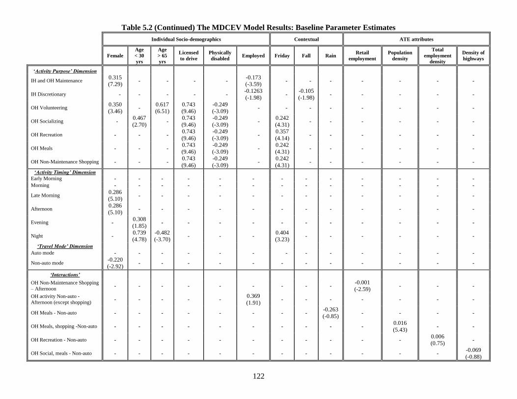
122
Table 5.2 (Continued) The MDCEV Model Results: Baseline Parameter Estimates
Individual Socio-demographics Contextual ATE attributes
Female
Age
< 30
yrs
Age
> 65
yrs
Licensed
to drive
Physically
disabled Employed Friday Fall Rain
Retail
employment
Population
density
Total
employment
density
Density of
highways
‘Activity Purpose’ Dimension
IH and OH Maintenance 0.315
(7.29) - - - -
-0.173
(-3.59) - - - - - - -
IH Discretionary - - - - - -0.1263
(-1.98) -
-0.105
(-1.98) - - - - -
OH Volunteering 0.350
(3.46) -
0.617
(6.51)
0.743
(9.46)
-0.249
(-3.09) - - - - - - - -
OH Socializing - 0.467
(2.70) -
0.743
(9.46)
-0.249
(-3.09) -
0.242
(4.31) - - - - - -
OH Recreation - - - 0.743
(9.46)
-0.249
(-3.09) -
0.357
(4.14) - - - - - -
OH Meals - - - 0.743
(9.46)
-0.249
(-3.09) -
0.242
(4.31) - - - - - -
OH Non-Maintenance Shopping - - - 0.743
(9.46)
-0.249
(-3.09) -
0.242
(4.31) - - - - - -
‘Activity Timing’ Dimension Early Morning - - - - - - - - - - - - - Morning - - - - - - - - - - - - -
Late Morning 0.286
(5.10) - - - - - - - - - - - -
Afternoon 0.286
(5.10) - - - - - - - - - - - -
Evening - 0.308
(1.85) - - - - - - - - - - -
Night - 0.739
(4.78)
-0.482
(-3.70) - - -
0.404
(3.23) - - - - - -
‘Travel Mode’ Dimension Auto mode - - - - - - - - - - - - -
Non-auto mode -0.220
(-2.92) - - - - - - - - - - - -
‘Interactions’
OH Non-Maintenance Shopping
– Afternoon - - - - - - - - -
-0.001
(-2.59) - - -
OH activity Non-auto -
Afternoon (except shopping) - - - - -
0.369
(1.91) - - - - - - -
OH Meals - Non-auto - - - - - - - - -0.263
(-0.85) - - - -
OH Meals, shopping -Non-auto - - - - - - - - - - 0.016
(5.43) - -
OH Recreation - Non-auto - - - - - - - - - - - 0.006
(0.75) -
OH Social, meals - Non-auto - - - - - - - - - - - - -0.069
(-0.88)
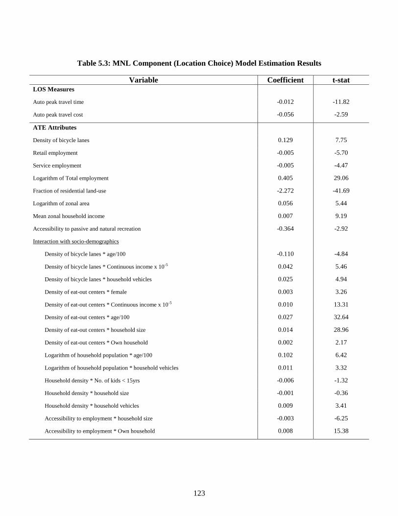
123
Table 5.3: MNL Component (Location Choice) Model Estimation Results
Variable Coefficient t-stat
LOS Measures
Auto peak travel time -0.012 -11.82
Auto peak travel cost -0.056 -2.59
ATE Attributes
Density of bicycle lanes 0.129 7.75
Retail employment -0.005 -5.70
Service employment -0.005 -4.47
Logarithm of Total employment 0.405 29.06
Fraction of residential land-use -2.272 -41.69
Logarithm of zonal area 0.056 5.44
Mean zonal household income 0.007 9.19
Accessibility to passive and natural recreation -0.364 -2.92
Interaction with socio-demographics
Density of bicycle lanes * age/100 -0.110 -4.84
Density of bicycle lanes * Continuous income x 10-5 0.042 5.46
Density of bicycle lanes * household vehicles 0.025 4.94
Density of eat-out centers * female 0.003 3.26
Density of eat-out centers * Continuous income x 10-5 0.010 13.31
Density of eat-out centers * age/100 0.027 32.64
Density of eat-out centers * household size 0.014 28.96
Density of eat-out centers * Own household 0.002 2.17
Logarithm of household population * age/100 0.102 6.42
Logarithm of household population * household vehicles 0.011 3.32
Household density * No. of kids < 15yrs -0.006 -1.32
Household density * household size -0.001 -0.36
Household density * household vehicles 0.009 3.41
Accessibility to employment * household size -0.003 -6.25
Accessibility to employment * Own household 0.008 15.38
124
CHAPTER 6 POLICY ANALYSIS
6.1 Background
In Chapters 2 through 5, we have discussed the formulation of econometric models for
analyzing multidimensional choices. Specifically, in the current dissertation, we
discussed the development of the following econometric frameworks (the choice
dimension is indicated in parenthesis): (1) multinomial logit model (reason for move) and
a grouped logit model (residential stay duration preceding the move), (2) copula-based
binary logit model (residential location) and log-linear regression (VMT), (3) copula-
based nested logit model (combination of residential location and vehicle type) and log-
linear regression (annual vehicle mileage for each vehicle type) and (4) joint multiple
discrete continuous extreme value model (activity type, travel mode, time of day
combination as the discrete component and activity duration as continuous component)
and multinomial logit model (MNL) with sampling of alternatives (activity location). The
preceding chapters, in addition to formulating these models, discuss how these models
have been estimated for actual data sets. The results from these exercises provide useful
insights on examining the different multinomial choice contexts. In fact, the results
presented clearly highlight the importance of incorporating direct (causal) and indirect
(self-selection) effects of travel environment on the choices considered from intuitive and
statistical perspectives (see goodness of fit measures for each of the models formulated).
In the current chapter, we undertake a series of policy analysis exercise that
further reinforce the importance of accommodating direct (causal) and indirect (self-
selection) effects of travel environment. The rest of the chapter is organized as follows.
Section 6.2 through 6.5 presents details of the policy exercises undertaken for each
multidimensional choice framework considered in the dissertation and discuss the
implication of their results. Section 6.6 concludes the chapter by summarizing the
insights across the different choice contexts.
125
6.2 Household residential relocation decision
In Chapter 2, three different model structures were estimated to facilitate comparisons
and to evaluate the efficacy of employing the correlated joint model system proposed for
modeling residential location decisions. The three models are:
A simple multinomial logit model for reason to move and an independent grouped
response model for duration of stay, referred to as the Independent Multinomial
Ordered (IMO) model
A random coefficients multinomial logit model for reason to move and an
independent random coefficients grouped response model for duration of stay,
referred to as the Independent Random Multinomial Ordered (IRMO) model
A random coefficients multinomial logit model for reason to move and a
correlated random coefficients grouped response model for duration of stay,
referred to as the Correlated Random Multinomial Ordered (CRMO) model.
6.2.1 Elasticity effects computation
The parameters on the exogenous variables for the CRMO model presented in Tables 6.1
and 6.2 do not directly provide the magnitude of the effects of the variables on the
probability of each choice dimension. To better understand the effects of various factors
on the reason to move and duration of stay choices, aggregate level elasticity effects were
computed. To discuss how we computed elasticities, let us briefly revisit the probability
expression from Section 2.4.
The probability of an individual q choosing to move for reason k at the tth
choice
occasion, conditional on qk and qk for each (and all) k, is given by:
' ' '( )
1 1 2 2 ' ' '( )
1
| ( , , , ,... , )
xk qk qt qk
qkt q q q q qK qK K xk qk qt qk
k
eP
e
(6.1)
Similarly, conditional on qk and qk , the probability of an individual q choosing to stay
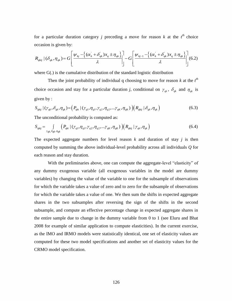
126
for a particular duration category j preceding a move for reason k at the tth
choice
occasion is given by:
' ' ' '
1( ) ( )| ( , )
kj k qk q qk kj k qk q qk
qktj qk qk
x xR G G
(6.2)
where G(.) is the cumulative distribution of the standard logistic distribution
Then the joint probability of individual q choosing to move for reason k at the tth
choice occasion and stay for a particular duration j, conditional on qk , qk and
qk is
given by :
1 1 2 2| ( , , ) | ( , , , ,... , ) | ,qktj qk qk qk qkt q q q q qK qK qktj qk qkS P R (6.3)
The unconditional probability is computed as:
1 1 2 2,,
| ( , , , ,... , ) | ,qktj qkt q q q q qK qK qktj qk qk
qk qk qk
S P R
(6.4)
The expected aggregate numbers for level reason k and duration of stay j is then
computed by summing the above individual-level probability across all individuals Q for
each reason and stay duration.
With the preliminaries above, one can compute the aggregate-level “elasticity” of
any dummy exogenous variable (all exogenous variables in the model are dummy
variables) by changing the value of the variable to one for the subsample of observations
for which the variable takes a value of zero and to zero for the subsample of observations
for which the variable takes a value of one. We then sum the shifts in expected aggregate
shares in the two subsamples after reversing the sign of the shifts in the second
subsample, and compute an effective percentage change in expected aggregate shares in
the entire sample due to change in the dummy variable from 0 to 1 (see Eluru and Bhat
2008 for example of similar application to compute elasticities). In the current exercise,
as the IMO and IRMO models were statistically identical, one set of elasticity values are
computed for these two model specifications and another set of elasticity values for the
CRMO model specification.
127
6.2.2 Elasticity effects
A comparison of elasticity measures across these model specifications sheds further light
on the importance of considering error correlation structures in simultaneously modeling
the reason to move and stay duration. The results for the move reason and duration
component are discussed subsequently.
6.2.2.1 Reason to move choice
Elasticity computations for the reason to move choice are shown in Table 6.1. The
interpretation of the elasticity values themselves is quite straightforward. For instance,
the table suggests that the probability of a female moving for personal family reasons is
about 28 percent more than that for males, all else being equal. On the other hand, the
probability of males moving for education/employment reasons exceeds that for females
by about 7.5 percent. The key finding from this table is that the CRMO model offers
elasticity estimates that differ by at least a few percentage points for all exogenous factors
considered in the model system. Also, several variables are found to have large impacts
on the probability of the reason to move. For example, an individual in a family-
household is less likely to move for education/employment reasons by nearly 95 percent.
The probability of an individual in a non-family household moving within the 20 year
period covered by the survey is less than that for an individual in a family household by
nearly 90 percent. Those who commute by walk exhibit a probability of moving for
education/employment reasons exceeding that for non-walk commuters by more than 75
percent. However, the probability of their moving for accommodation or surrounding
vicinity related reasons is substantially smaller than that for non-walk commuters.
6.2.2.2 Duration of stay choice
In Table 6.2, elasticity computations are provided for the duration of stay choice and the
differences between elasticity measures derived from the IMO/IRMO model and those
derived from the CRMO model are more striking. It is found that, in comparison to
128
males, females are more likely to stay for less than two years at a single location by
nearly 20 percent. In the case of household size, it is interesting to note that the aggregate
elasticity value is of a different magnitude and sign for the 2-5 year stay category. While
the IMO/IMRO models suggest that the probability of staying 2-5 years at a single
location increases with household size, the CRMO model suggests that this probability
actually decreases with an increase in household size. Indeed, one would expect that the
probability of stay duration being short (2-5 years may be considered a short stay) would
decrease with an increase in household size. Similar sign reversals are seen for the
variables representing home ownership and number of rooms in the home, in the 2-5 year
stay category. This category probably represents a transition point between short-term
stays and longer-term stays and hence the model that accounts for the presence of
common unobserved factors (error correlations) is offering elasticity measures
substantially different than those obtained from models that do not account for such
factors. These sign reversals are also seen for commute-related variables, where the
IMO/IMRO models suggest that the probability of staying 2-5 years (short stay) is lower
for public transportation and walk users. However, the CRMO model suggests that the
probability of staying 2-5 years is actually higher, albeit by rather small amounts, for
these alternate mode users. The CRMO model suggests greater negative differentials in
the longer stay duration category of greater than 10 years. For example, according to the
IMO/IRMO model, the probability of bicycle commuters staying more than 10 years at
the same location is lower than that for others by 3 percent; the corresponding differential
(elasticity) is 5.2 percent in the CRMO model.
6.3 Residential location and VMT
In Chapter 3, we formulated a copula based approach to model residential neighborhood
choice and daily household vehicle miles of travel (VMT). The situation can be cast in
the form of Roy‟s (1951) endogenous switching model system (see Maddala, 1983;
Chapter 9), which takes the following form:
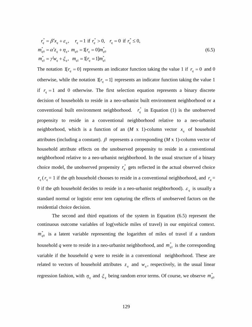
129
*
11
*
1
*
00
*
0
***
]1[1 ,
]0[1 ,
,0 if 0 ,0 if 1 ,
qqqqqq
qqqqqq
qqqqqqq
mrmwm
mrmzm
rrrrxr
(6.5)
The notation ]0[1 qr represents an indicator function taking the value 1 if 0qr and 0
otherwise, while the notation ]1[1 qr represents an indicator function taking the value 1
if 1qr and 0 otherwise. The first selection equation represents a binary discrete
decision of households to reside in a neo-urbanist built environment neighborhood or a
conventional built environment neighborhood. *
qr in Equation (1) is the unobserved
propensity to reside in a conventional neighborhood relative to a neo-urbanist
neighborhood, which is a function of an (M x 1)-column vector qx of household
attributes (including a constant). represents a corresponding (M x 1)-column vector of
household attribute effects on the unobserved propensity to reside in a conventional
neighborhood relative to a neo-urbanist neighborhood. In the usual structure of a binary
choice model, the unobserved propensity *
qr gets reflected in the actual observed choice
qr ( qr = 1 if the qth household chooses to reside in a conventional neighborhood, and qr =
0 if the qth household decides to reside in a neo-urbanist neighborhood). q is usually a
standard normal or logistic error tem capturing the effects of unobserved factors on the
residential choice decision.
The second and third equations of the system in Equation (6.5) represent the
continuous outcome variables of log(vehicle miles of travel) in our empirical context.
*
0qm is a latent variable representing the logarithm of miles of travel if a random
household q were to reside in a neo-urbanist neighborhood, and *
1qm is the corresponding
variable if the household q were to reside in a conventional neighborhood. These are
related to vectors of household attributes qz and qw , respectively, in the usual linear
regression fashion, with q and q being random error terms. Of course, we observe *
0qm

130
in the form of 0qm only if household q in the sample is observed to live in a neo-urbanist
neighborhood. Similarly, we observe *
1qm in the form of 1qm only if household q in the
sample is observed to live in a conventional neighborhood.
The observed data for each household in the switching model of Equation (6.5) is
its chosen residence location and the VMT given the chosen residential location. That is,
we observe if 0qr or 1qr for each q, so that either 0qm or 1qm is observed for each
q. We do not observe the data pair ),( 10 qq mm for any household q. However, using the
switching model, we would like to assess the impact of the neighborhood on VMT. In
the social science terminology, we would like to evaluate the expected gains (i.e., VMT
increase) from the receipt of treatment (i.e., residing in a conventional neighborhood).
Heckman and Vytlacil, 2000 and Heckman et al., 2001 define a set of measures to study
the influence of treatment, two important such measures being Average Treatment Effect
(ATE) and the Effect of Treatment on the Treated (TT). We discuss these below, and
propose two new measures labeled “Effect of Treatment on the Non-Treated (TNT)” and
“Effect of Treatment on the Treated and Non-treated (TTNT)”.
6.3.1 Treatment Effects
The ATE measure provides the expected VMT increase for a random household if
it were to reside in a conventional neighborhood as opposed to a neo-urbanist
neighborhood. The ATE is estimated as:
Q
q
qq zwQ 1
22 )2/ˆˆexp()2/ˆˆexp(1
ATE (6.6)
Heckman and Vytlacil (2000) propose a “Treatment on the Treated” or TT
measure that captures the expected VMT increase for a household randomly picked from
the pool located in a conventional neighborhood if it were instead located in a neo-
urbanist neighborhood (in social science parlance, it is the average impact of “treatment
on the treated”; see Heckman and Vytlacil, 2005). The TT measure can be estimated as
follows:
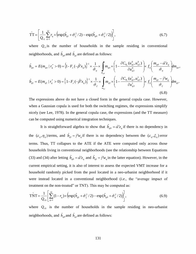
131
, )2/ˆˆexp()2/ˆˆexp(1
TT1
2
0
2
1
1
Q
q
qqq
r
bbrQ
(6.7)
where 1rQ is the number of households in the sample residing in conventional
neighborhoods, and 0ˆ
qb and 1ˆ
qb are defined as follows:
,ˆ
ˆ),(1
ˆ
1)ˆ(-1)0|(ˆ 0
0
2
0
2
0
11* 0
0
qo
q
m
qoqqqoqo dmzm
fu
uuCmxFrmEb
q
.ˆ
ˆ),(1
ˆ
1)ˆ(-1 )0|(ˆ
1
1
1
2
1
2
1
1
1
1*
111
1
q
q
m
qqqqq dmwm
fu
uuCmxFrmEb
q
(6.8)
The expressions above do not have a closed form in the general copula case. However,
when a Gaussian copula is used for both the switching regimes, the expressions simplify
nicely (see Lee, 1978). In the general copula case, the expressions (and the TT measure)
can be computed using numerical integration techniques.
It is straightforward algebra to show that qq zb ˆˆ0 if there is no dependency in
the ),( qq terms, and qq wb ˆˆ1 if there is no dependency between the ),( qq error
terms. Thus, TT collapses to the ATE if the ATE were computed only across those
households living in conventional neighborhoods (see the relationship between Equations
(33) and (34) after letting qq zb ˆˆ0 and qq wb ˆˆ
1 in the latter equation). However, in the
current empirical setting, it is also of interest to assess the expected VMT increase for a
household randomly picked from the pool located in a neo-urbanist neighborhood if it
were instead located in a conventional neighborhood (i.e., the “average impact of
treatment on the non-treated” or TNT). This may be computed as:
, )2/ˆˆexp()2/ˆˆexp()1(1
TNT1
2
0
2
1
0
Q
q
qqq
r
hhrQ
(6.9)
where 0rQ is the number of households in the sample residing in neo-urbanist
neighborhoods, and 0ˆ
qh and 1ˆ
qh are defined as follows:
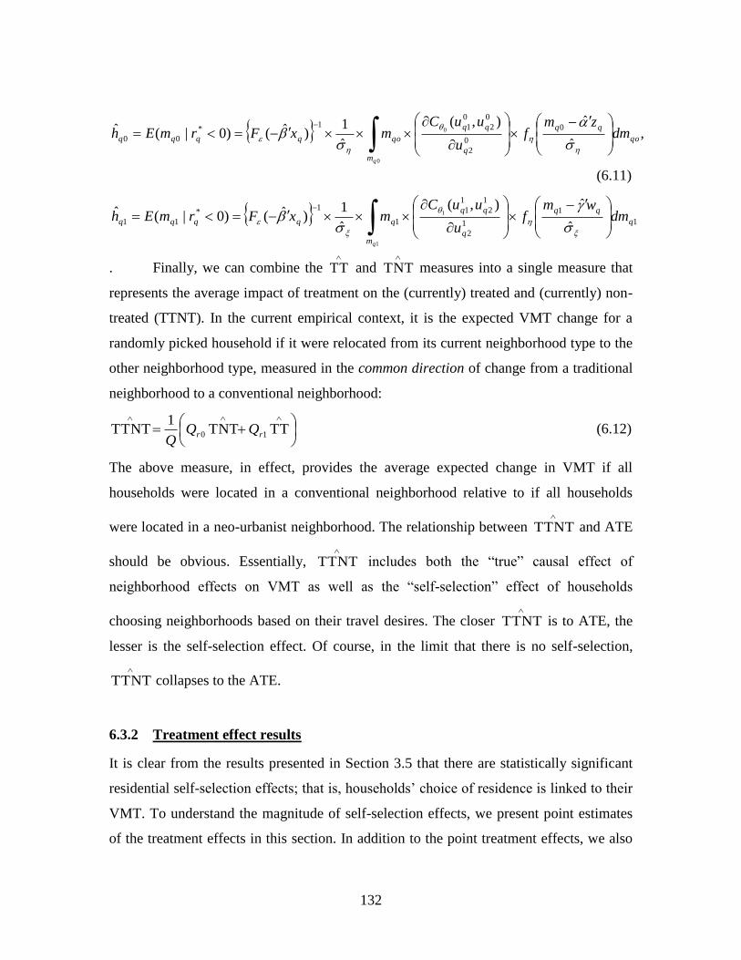
132
,ˆ
ˆ),(
ˆ
1)ˆ()0|(ˆ 0
0
2
0
2
0
11*
00
0
0
qo
q
m
qoqqqq dmzm
fu
uuCmxFrmEh
q
(6.11)
1
1
1
2
1
2
1
1
1
1*
11ˆ
ˆ),(
ˆ
1)ˆ()0|(ˆ 1
1
q
q
m
qqqqq dmwm
fu
uuCmxFrmEh
q
. Finally, we can combine the
TT and
TNT measures into a single measure that
represents the average impact of treatment on the (currently) treated and (currently) non-
treated (TTNT). In the current empirical context, it is the expected VMT change for a
randomly picked household if it were relocated from its current neighborhood type to the
other neighborhood type, measured in the common direction of change from a traditional
neighborhood to a conventional neighborhood:
TTTNT1
TTNT 10 rr QQQ
(6.12)
The above measure, in effect, provides the average expected change in VMT if all
households were located in a conventional neighborhood relative to if all households
were located in a neo-urbanist neighborhood. The relationship between
TTNT and ATE
should be obvious. Essentially,
TTNT includes both the “true” causal effect of
neighborhood effects on VMT as well as the “self-selection” effect of households
choosing neighborhoods based on their travel desires. The closer
TTNT is to ATE, the
lesser is the self-selection effect. Of course, in the limit that there is no self-selection,
TTNT collapses to the ATE.
6.3.2 Treatment effect results
It is clear from the results presented in Section 3.5 that there are statistically significant
residential self-selection effects; that is, households‟ choice of residence is linked to their
VMT. To understand the magnitude of self-selection effects, we present point estimates
of the treatment effects in this section. In addition to the point treatment effects, we also
133
estimate large sample standard errors for the treatment effects using 1000 bootstrap
draws. This involves drawing from the asymptotic distributions of parameters appearing
in the treatment effect, and computing the standard deviation of the simulated treatment
effect values.
The results are presented in Table 6.3 for the Independence-Independence (I-I)
model and the three copula models with the best data fit, corresponding to the FGM-Joe
(FG-J), Frank-Joe (F-J), and the Frank -Frank (F-F) copula models. Of course, the results
from the traditional Gaussian-Gaussian (G-G) model are literally identical to the results
from the I-I model, since the correlation parameters in the G-G model are small and very
insignificant. The results show substantial variation in the treatment measures across
models, except for the F-J and F-F models which provide similar results (this is not
surprising, since the model parameters and log-likelihood values at convergence for these
two models are almost the same, as discussed earlier in Section 3.5.2). According to the
I-I model, a randomly selected household will have about the same VMT regardless of
whether it is located in a conventional or neo-urbanist neighborhood (see the small and
statistically insignificant ATE estimate for the I-I model). On the other hand, the other
copula models indicate that there is indeed a statistically significant impact of the built
environment on VMT. For instance, the best-fitting F-F model indicates that a randomly
picked household will drive about 21 vehicle-miles per day more if in a conventional
neighborhood relative to a neo-urbanist neighborhood. The important message here is
that ignoring sample selection can lead to an underestimation or an overestimation of
built environment effects (the general impression is that ignoring sample selection can
only lead to an overestimation of built environment effects). Further, one needs to
empirically test alternative copulas to determine which structure provides the best data
fit, rather than testing the presence or absence of sample selection using normal
dependency structures.
The results also show statistically significant variations in the other treatment
effects between the I-I model and the non I-I models. The
TT and
TNT measures from
the non I-I models reflect, as expected, that a household choosing to locate in a certain
134
kind of neighborhood travels more in its chosen environment relative to an
observationally equivalent random household. Thus, if a randomly picked household in a
conventional neighborhood were to be relocated to a neo-urbanist neighborhood, the
household‟s VMT is estimated to decrease by about 42 miles. Similarly, if a randomly
picked household in a neo-urbanist neighborhood were to be relocated to a conventional
neighborhood, the household‟s VMT is estimated to decrease by about 31 miles. On the
other hand, if a randomly picked household that is indifferent to neighborhood type is
moved from a conventional to a neo-urbanist neighborhood, the household‟s VMT is
estimated to decrease by about 21 miles (which is, of course, the ATE measure).
The
TTNT measure is a weighted average of the
TT and
TNT measures, and
shows that there would be a decrease of about 25 vehicle miles of travel per day if all
households in the population (as represented by the estimation sample) were located in a
neo-urbanist neighborhood rather than a conventional neighborhood. When compared to
the average VMT of 58 miles, the implication is that one may expect a VMT reduction of
about 43% by redesigning all neighborhoods to be of the neo-urbanist neighborhood
type.18
Finally, the
TTNT measure for the best F-F copula model shows that about 87%
of the VMT difference between households residing in conventional and neo-urbanist
neighborhoods is due to “true” built environment effects, while the remainder is due to
residential self-selection effects. However, most importantly, it is critical to note that
failure to accommodate the self-selection effect leads to a substantial underestimation of
the “true” built environment effect (see the ATE for the I-I model of 0.49 miles relative
to the ATE for the F-F model of 21.37 miles.
18 Note that we are simply presenting this figure as a way to provide a magnitude effect of VMT reduction
by designing urban environments to be of the neo-urbanist kind. In practice, different neighborhoods may
be redesigned to different extents to make them less auto-dependent. Further, in a democratic society,
demand will (and should) fuel supply. Thus, as long as there are individuals who prefer to live in a
conventional setting, there will be developers to provide that option.
135
6.4 Household vehicle fleet composition and usage choices
In Chapter 4, a simultaneous model of residential location choice, vehicle count and type
choice, and vehicle usage is presented with a view to capture the potential effects of the
presence of common unobserved factors that may jointly impact these choice dimensions.
The research effort employs the structure of the copula-based joint GEV-based logit –
regression modeling framework to jointly model the choice dimensions. To demonstrate
the applicability of the model system developed in the Chapter 4, the model results
presented in Table 4.2 are employed to predict changes in residential location, vehicle
type shares, and vehicle usage.
6.4.1 Policy exercise
In this exercise, changes in the choice dimensions are examined as a function of changes
in exogenous factors. In particular, the impacts of changes in household demographics,
built environment variables, and local transportation measures are examined in this
simple simulation exercise. The specific changes in exogenous factors considered are
increasing household size,
number of employed individuals,
number of females by unity,
increasing land use mix value of the neighborhood by 25 percent, and
increasing the number of zones accessible by bicycle within a six mile radius by
50 percent.
The results of the application exercise are presented in Table 6.4. The table
shows changes in shares and usage by residential location and vehicle type for the Frank
copula model and the model of independence that sets all dependency parameters to zero.
6.4.2 Results
In general, it is found that the sensitivity (changes in shares and usage) provided by the
Frank copula model differs from that of the model of independence. While some
136
differences are small, there are some that are quite substantial (e.g., effect of household
size increase on usage of van), suggesting that ignoring dependency among choice
dimensions could result in serious over- or under-estimation of impacts of changes in
exogenous variables.
Larger household sizes and an increase in number of employed individuals result
in a shift towards conventional neighborhoods, although an increase in the
number of females results in a shift towards neo-urbanist neighborhoods.
Similarly, improvements in land use density and bicycle accessibility result in
shifts towards neo-urbanist neighborhoods.
An increase in the number of employed individuals increases the share of pickup
trucks significantly, while resulting in a decrease across all other vehicle types,
including the choice of no vehicle purchase. On the other hand, an increase in the
number of females reduces the share of all vehicle types, except that for compact
and large sedans whose shares increase.
Increases in household sizes are met with a higher likelihood of not making a
vehicle purchase suggesting that households reach a vehicle ownership saturation
point beyond which they do not acquire additional vehicles even when an
additional person enters the household.
Built environment and transportation accessibility are associated with a decreased
share of pickup trucks and slight increases in shares of all other vehicle types,
including the choice of not acquiring a vehicle. In fact, an increase in the number
of zones accessible by bicycle results in reduction of all vehicle types leading to
an increase in the share of the “no vehicle” alternative.
It is interesting to note that the Frank copula model shows consistently different levels of
sensitivity in vehicle usage compared to the model of independence. It is apparent that
ignoring unobserved dependency among choice dimensions (indirect effects or self-
selection) may result in biased estimation of the potential impacts (benefits) of enhanced
non-motorized transport accessibility.
137
6.5 Activity participation decisions
In Chapter 5, we presented a joint model system of five choice dimensions, activity type
choice, activity time of day choice (treated as discrete time intervals), mode choice,
destination choice, and activity duration (continuous choice dimension). Specifically, the
MDCEV model is used to represent activity participation (discrete choice) and time use
(continuous choice) for different types of activities at different time periods of the day by
different travel modes. The activity location choice is modeled using a multinomial logit
(MNL) model nested within the MDCEV framework. The major objective of this
research effort was to develop a unified model of activity-travel and location choices and
time use that would allow one to examine the influence of level of service measures and
activity-travel environment (ATE) attributes on these choice dimensions in an integrated
manner. To demonstrate the capabilities of the model system presented in Chapter 5, we
undertake a series of policy exercises that are discussed subsequently.
6.5.1 Policy exercise details
The econometric model formulated and estimated in Chapter 5 was used to examine the
impacts of the following scenarios on activity and time use behavior:
Doubling travel cost across all time periods
Doubling travel cost during peak periods
Doubling travel cost for auto mode
Doubling travel time across all time periods
Doubling travel time during peak periods
Doubling travel time by auto mode
Logsum variables computed using the activity destination choice MNL model were used
as explanatory variables in the MDCEV model to predict individual‟s participation in and
time allocation to activities by activity purpose, timing, and mode (see the formulation in
Section 5.2.2 for definition of logsum). For each policy scenario, logsum variables were
computed for all 60 OH discretionary activity purpose, timing, and mode combinations
138
(for use in the base case prediction), and then updated for the specific timing or travel
mode categories for which the policy applied (for the policy case prediction). The
prediction using MDCEV was carried out for all individuals in the sample using 1000
replications of the error term draws for each individual. Additional details about the
forecasting procedure using the MDCEV model are provided in Pinjari and Bhat (2009b).
6.5.2 Policy exercise results
The forecasts under alternative scenarios are presented in Table 6.5. Specifically,
the influence of each policy is reported as an aggregate percent change in the amount of
time invested in maintenance activities, in-home discretionary activities, and out-of-home
discretionary activities by purpose, time of day, and mode (relative to the base case). The
important findings from the policy exercise are highlighted below:
Increases in travel cost lead to reduced out-of-home activity engagement and
slight increases in in-home activity engagement.
Increases in travel cost during the peak period impact volunteer, eat-meal, and
recreation activities more than others, and reduce peak period activity engagement
while increasing off-peak activity engagement.
Increases in auto travel costs and times reduce the use of auto mode for activity
engagement and contribute to enhanced mode shares for non-auto modes.
In general, travel time increases appear to have larger impacts than travel costs,
suggesting that individuals are more time-sensitive when making activity-travel
choices.
In terms of the modal impact, it appears that all day travel cost or time increases
have a greater impact than a time-specific peak-period travel cost or time
increase.
It appears that individuals are more likely to respond to price and time signals that
cover an entire day as opposed to those that are narrower in the time band of
influence.
139
In general, the results provide indications along expected lines. To summarize, the policy
simulation results clearly show that the model is effective in capturing the responses of
individuals to system changes in a unifying framework.
6.6 Summary
In the current chapter, we present a variety of policy exercises undertaken using the
econometric models formulated and estimated in Chapter 2 through 5. In fact, we
summarize the results of the wide ranging exercise that includes computing different
policy measures including: (a) aggregate elasticicties, (b) treatment effects and (c)
response to incremental changes to exogenous variables and (d) sensitivity to policy
scenarios. The results, in this chapter, further corroborate the findings from Chapter 2
through 5 that it is important to incorporate the influence of direct and indirect effects of
travel environment on travel demand.
140
Table 6.1: Elasticity Values for the Move Reason Choice
Alternatives
Characteristics
Fam Edu Acc SuVi Two Oth NM
IMO/IRMO CRMO IMO/IRMO CRMO IMO/IRMO CRMO IMO/IRMO CRMO IMO/IRMO CRMO IMO/IRMO CRMO IMO/IRMO CRMO
Individual characteristics
Gender
Female 28.2 26.2 -8.4 -7.5 -6.9 -6.5 -6.3 -6.5 -7.4 -6.5 -6.4 -6.5 -6.5 -6.8
Age
Age 31 - 45 years -14.0 -13.0 -13.2 -12.5 7.3 7.4 8.0 8.6 7.7 7.4 7.2 7.6 6.9 7.9
Age > 45 years -69.0 -66.4 -63.1 -63.1 38.0 39.4 40.4 44.8 41.6 40.1 35.8 39.5 33.6 38.6
Employed -12.8 -10.6 -11.4 -9.6 7.8 10.9 -12.3 -11.7 8.3 5.8 23.4 19.6 -13.0 -13.9
Household characteristics
Household size 2.9 3.0 2.0 2.3 2.8 3.1 2.2 2.7 3.0 3.0 2.6 3.2 -61.9 -61.3
Household Type (Single
person household is base)
Family household 28.5 27.2 -97.5 -94.4 24.5 25.5 -83.1 -81.0 25.4 24.9 24.2 26.8 22.6 27.3
Non-family household 4.4 4.4 3.1 3.3 4.3 4.6 3.4 4.2 4.5 4.5 3.9 4.9 -90.2 -89.0
Household tenure (Rent is
base)
Own household -2.1 -8.0 -75.5 -75.5 26.1 31.6 -35.8 -38.6 28.0 31.8 25.3 32.3 21.9 30.7
Commute characteristics
Mode to work (Car is base)
Public transportation -8.8 -8.5 13.5 17.2 -8.4 -8.4 10.7 8.4 -8.7 -8.2 33.9 26.1 -7.4 -8.7
Bicycle -55.4 -53.3 44.9 45.4 14.4 19.0 -29.8 -32.3 17.8 19.5 42.2 30.2 -50.8 -54.8
Walk 3.5 1.5 73.6 76.6 -41.9 -38.3 -58.1 -60.7 6.9 3.9 6.4 5.0 7.0 7.0
Distance to work
Above 10 km 3.6 3.4 2.6 2.6 3.7 3.8 3.0 3.5 3.8 3.6 3.5 4.2 -82.1 -81.0
141
Table 6.2: Elasticity Values for the Duration of Stay Choice
Alternatives
Characteristics
< 2years 2 - 5 years 5 - 10 years > 10 years
IMO/IRMO
CRMO IMO/IRM
O CRMO
IMO/IRMO
CRMO IMO/IRM
O CRMO
Individual characteristics
Gender
Female 16.4 19.5 -1.8 1.8 -14.0 -13.5 -2.5 -4.4
Age 0.2 0.2 -0.1 -0.1 0.1 0.0 0.1 0.1
Household characteristics
Household size -18.0 -20.5 1.0 -4.3 17.7 16.8 3.3 6.6
Household Type (Single person
household is base)
Non-family household 75.8 83.8 -17.5 -4.6 -47.7 -43.2 -7.7 -11.9
Household tenure (Rent is
base)
Own household -23.4 -19.3 1.8 -2.5 23.1 14.1 4.7 5.3
Number of rooms in the house
1 - 2 rooms 28.6 31.4 -5.1 1.1 -24.5 -21.0 -4.3 -6.7
Transportation characteristics
Mode to work (Car is base)
Public transportation 14.6 15.7 -2.0 1.4 -13.6 -11.3 -2.5 -3.9
Bicycle 21.5 27.1 -3.4 0.8 -16.9 -16.8 -3.0 -5.2
Distance to work
Above 10 km 29.4 31.9 -4.9 1.9 -26.9 -22.2 -5.1 -7.6
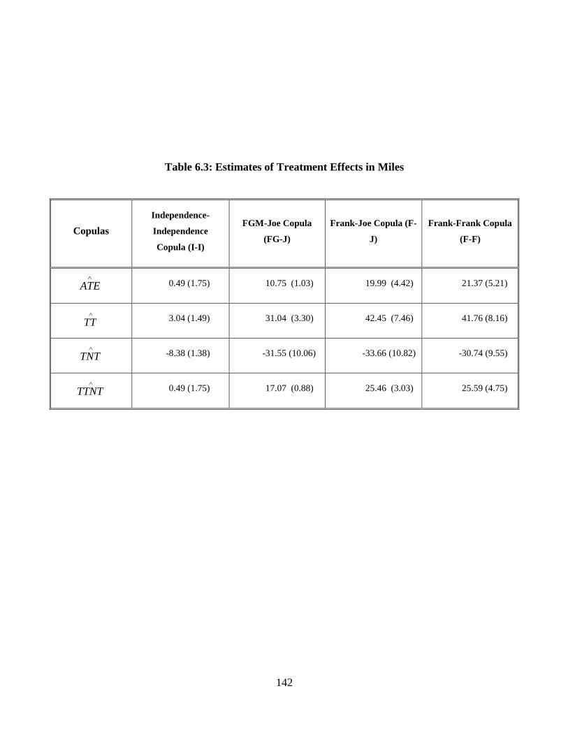
142
Table 6.3: Estimates of Treatment Effects in Miles
Copulas
Independence-
Independence
Copula (I-I)
FGM-Joe Copula
(FG-J)
Frank-Joe Copula (F-
J)
Frank-Frank Copula
(F-F)
ATE
0.49 (1.75) 10.75 (1.03) 19.99 (4.42) 21.37 (5.21)
TT
3.04 (1.49) 31.04 (3.30) 42.45 (7.46) 41.76 (8.16)
TNT
-8.38 (1.38) -31.55 (10.06) -33.66 (10.82) -30.74 (9.55)
TTNT
0.49 (1.75) 17.07 (0.88) 25.46 (3.03) 25.59 (4.75)
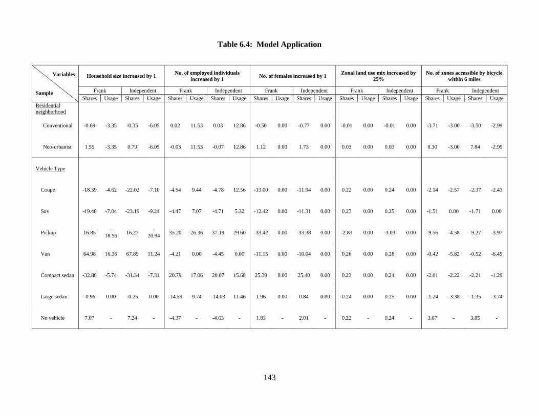
143
Table 6.4: Model Application
Variables
Sample
Household size increased by 1 No. of employed individuals
increased by 1 No. of females increased by 1
Zonal land use mix increased by
25%
No. of zones accessible by bicycle
within 6 miles
Frank Independent Frank Independent Frank Independent Frank Independent Frank Independent
Shares Usage Shares Usage Shares Usage Shares Usage Shares Usage Shares Usage Shares Usage Shares Usage Shares Usage Shares Usage
Residential neighborhood
Conventional -0.69 -3.35 -0.35 -6.05 0.02 11.53 0.03 12.86 -0.50 0.00 -0.77 0.00 -0.01 0.00 -0.01 0.00 -3.71 -3.00 -3.50 -2.99
Neo-urbanist 1.55 -3.35 0.79 -6.05 -0.03 11.53 -0.07 12.86 1.12 0.00 1.73 0.00 0.03 0.00 0.03 0.00 8.30 -3.00 7.84 -2.99
Vehicle Type
Coupe -18.39 -4.62 -22.02 -7.10 -4.54 9.44 -4.78 12.56 -13.00 0.00 -11.94 0.00 0.22 0.00 0.24 0.00 -2.14 -2.57 -2.37 -2.43
Suv -19.48 -7.04 -23.19 -9.24 -4.47 7.07 -4.71 5.32 -12.42 0.00 -11.31 0.00 0.23 0.00 0.25 0.00 -1.51 0.00 -1.71 0.00
Pickup 16.85 -
18.56 16.27
-
20.94 35.20 26.36 37.19 29.60 -33.42 0.00 -33.38 0.00 -2.83 0.00 -3.03 0.00 -9.56 -4.58 -9.27 -3.97
Van 64.98 16.36 67.89 11.24 -4.21 0.00 -4.45 0.00 -11.15 0.00 -10.04 0.00 0.26 0.00 0.28 0.00 -0.42 -5.82 -0.52 -6.45
Compact sedan -32.86 -5.74 -31.34 -7.31 20.79 17.06 20.07 15.68 25.39 0.00 25.40 0.00 0.23 0.00 0.24 0.00 -2.01 -2.22 -2.21 -1.29
Large sedan -0.96 0.00 -0.25 0.00 -14.59 9.74 -14.03 11.46 1.96 0.00 0.84 0.00 0.24 0.00 0.25 0.00 -1.24 -3.38 -1.35 -3.74
No vehicle 7.07 - 7.24 - -4.37 - -4.63 - 1.83 - 2.01 - 0.22 - 0.24 - 3.67 - 3.85 -
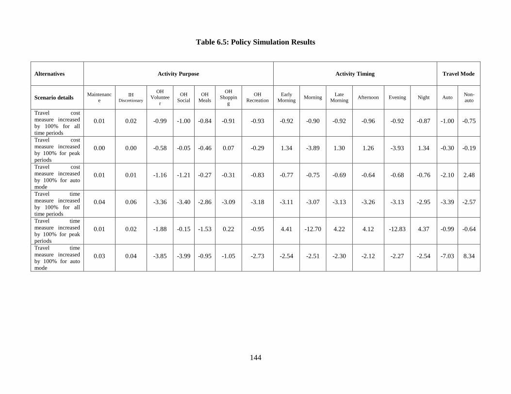
144
Table 6.5: Policy Simulation Results
Alternatives Activity Purpose Activity Timing Travel Mode
Scenario details Maintenanc
e IH
Discretionary
OH Voluntee
r
OH
Social
OH
Meals
OH Shoppin
g
OH
Recreation
Early
Morning Morning
Late
Morning Afternoon Evening Night Auto
Non-
auto
Travel cost
measure increased
by 100% for all
time periods
0.01 0.02 -0.99 -1.00 -0.84 -0.91 -0.93 -0.92 -0.90 -0.92 -0.96 -0.92 -0.87 -1.00 -0.75
Travel cost
measure increased
by 100% for peak
periods
0.00 0.00 -0.58 -0.05 -0.46 0.07 -0.29 1.34 -3.89 1.30 1.26 -3.93 1.34 -0.30 -0.19
Travel cost
measure increased
by 100% for auto
mode
0.01 0.01 -1.16 -1.21 -0.27 -0.31 -0.83 -0.77 -0.75 -0.69 -0.64 -0.68 -0.76 -2.10 2.48
Travel time
measure increased
by 100% for all
time periods
0.04 0.06 -3.36 -3.40 -2.86 -3.09 -3.18 -3.11 -3.07 -3.13 -3.26 -3.13 -2.95 -3.39 -2.57
Travel time
measure increased
by 100% for peak
periods
0.01 0.02 -1.88 -0.15 -1.53 0.22 -0.95 4.41 -12.70 4.22 4.12 -12.83 4.37 -0.99 -0.64
Travel time
measure increased
by 100% for auto
mode
0.03 0.04 -3.85 -3.99 -0.95 -1.05 -2.73 -2.54 -2.51 -2.30 -2.12 -2.27 -2.54 -7.03 8.34
145
CHAPTER 7 CONCLUSIONS AND DIRECTIONS FOR
FURTURE RESEARCH
7.1 Introduction
In the United States, a significant number of individuals depend on the auto mode of
transportation. The increasing auto travel, and its adverse environmental impacts (such as
traffic congestion and air pollution), has led, in the past decade, to a growing emphasis on
analyzing traveler behavior at the individual level rather than using direct statistical
projections of aggregate travel demand. In particular, the focus of travel demand
modeling has shifted from an underlying trip-based paradigm to an activity-based
paradigm, which treats travel as a demand derived from the need to participate in
activities dislocated in time and space (see Bhat and Koppelman, (1993)).
The activity-based framework considers travel as a means to pursue activities
distributed in time and space. The activity-based modeling framework essentially
attempts to replace the statistical travel prediction focus of the traditional trip-based
model framework with a more behavioral approach that explicitly recognizes the
fundamental role of activity participation as a precursor to travel. Essentially, the
objective of an activity-based travel modeling framework is to micro-simulate individual
activity and travel participation over the course of certain time interval, which usually is a
typical weekday.
It is widely recognized in transportation literature that an accurate characterization
of activity-travel patterns requires explicit consideration of the land-use and travel
environment. The influence of travel environment on travel behavior can be classified
into two categories: direct and indirect effects. The direct effect can be captured by
including travel environment related variables as exogenous variables in travel models.
However, accommodating only the direct effect in a travel model is far from simple
because the very travel environment attributes experienced by a decision maker
(individual or household) is a function of a suite of a priori travel related choices made
by the decision maker. The emphasis of the current dissertation is on recognizing the two
146
categories of travel environment effects and incorporating them within an econometric
framework.
The overall objective of the dissertation is to contribute to the growing literature
on integrated land-use activity-based model framework by developing econometric
models that can accommodate joint modeling of multidimensional choices. In particular,
the overall goal is to contribute to the debate on whether the empirically observed
association between the built environment and travel behavior-related variables is a true
reflection of underlying causality, or simply a spurious correlation attributable to the
intervening relationship between the built environment and the characteristics of people
who choose to live in particular built environments (or some combination of both these
effects). Towards this end, the current research effort contributes to the existing research
by (a) developing advanced econometric models for modeling multi-dimensional choices,
(b) estimating these models for travel data sets, and (c) undertaking policy analysis.
The current dissertation contributes substantially to integrated land-use activity
based modeling literature while simultaneously contributing methodologically by
formulating advanced econometric models. Specifically, we examine different modules
of an activity based framework. The empirical problems addressed in the dissertation
include: (1) reason for residential relocation and associated duration of stay, (2)
household residential location and daily vehicle miles travelled, (3) household residential
location, vehicle type and usage choices and (4) activity type, travel mode, time period of
day, activity duration and activity location.
The rest of the chapter is organized as follows. Section 7.2 through 7.5 discusses the
substantive and methodological contributions of the dissertation for each
multidimensional choice context examined in the dissertation. Section 7.6 concludes the
dissertation by offering directions for future research.
7.2 Household residential relocation decision
The major focus of the research effort presented in Chapter 2 is to understand household
residential relocation decisions. The study jointly models the reason for relocation and
147
the duration of stay at a location preceding the relocation, recognizing that the reason for
location may itself be an endogenous variable influenced by observed and unobserved
variables. The data for the empirical case study is drawn from a longitudinal data set
derived from a retrospective survey that was administered in the beginning of 2005 to
households drawn from a stratified sample of municipalities in the Zurich region of
Switzerland. The most important finding in the context of examining household
residential relocation decisions is that there are common unobserved factors affecting the
reason to move and the duration of stay choices. Other important findings and
recommendations include:
Several demographic, socio-economic, and commute related variables are found
to significantly influence the reason for move and the duration of stay
The study findings (based on estimation results and aggregate elasticity effects)
have implications for housing and labor policy. For example, those who own
households have a lower probability of moving for surrounding vicinity related
reasons than those renting their units. In other words, it appears that the potential
exists for improving existing surrounding vicinity conditions around rental
properties so that individuals unable to afford home ownership can enjoy the same
level of amenities and environment as those who are able to own their homes.
From a jobs-housing balance standpoint, having a mix of job opportunities located
close to residential neighborhoods may help increase the duration of stay for
individuals; reducing commute distance to a value of less than 10 km (in the
context of this Zurich based survey sample) fosters longer stay durations.
From a social standpoint, it appears that women are more prone to moving for
personal and family reasons; this may be reflective of the need for social support
systems for women who are affected by personal or family turmoil so that they do
not necessarily feel compelled to move away.
From a methodological perspective, the joint multinomial logit model and a
grouped logit model is the first instance of such a model developed in
econometrics literature.
148
7.3 Residential location and VMT
In Chapter 3, we apply a copula based approach to model residential neighborhood
choice and daily household vehicle miles of travel (VMT) using the 2000 San Francisco
Bay Area Household Travel Survey (BATS). The model considers the possibility of
households selecting their residence locations based on their travel needs i.e. the observed
VMT differences between households residing in neo-urbanist and conventional
neighborhoods cannot be attributed entirely to built environment variations between the
two neighborhoods types. A variety of copula-based models are estimated, including the
traditional Gaussian-Gaussian (G-G) copula model. The results indicate that using a
bivariate normal dependency structure suggests the absence of residential self-selection
effects. However, other copula structures reveal a high and statistically significant level
of residential self-selection, highlighting the potentially inappropriate empirical
inferences from using incorrect dependency structures.
Other important findings from the study include:
The best fit copula model developed in Chapter 3 estimates that self-selection
effects constitute about 17% of the VMT difference between neo-urbanist and
conventional households, while “true” built environment effects constitute the
remaining 83% of the VMT difference.
The results of this study indicate that, in the empirical context of the current
study, failure to accommodate residential self-selection effects can lead to a
substantial mis-estimation of the true built environment effects.
A randomly picked household will drive about 21 vehicle-miles per day more if
residing in a conventional neighborhood relative to a neo-urbanist neighborhood.
If a randomly picked household in a conventional neighborhood were to be
relocated to a neo-urbanist neighborhood, the household‟s VMT is estimated to
decrease by about 42 miles.
From a methodological standpoint, the copula approach introduced in this
dissertation happens to be the first instance of the application of copulas models
in transportation literature. In fact, this work has led to huge attention within the
149
transportation community as revealed by a multitude of papers employing copulas
(for example see Spissu et al.2009, Eluru et al., 2009, Portogese et al., 2009,
Sener and Bhat 2009, Sener et al., 2009, Lamondia and Bhat 2009, Rana et al.,
2010)
Finally, the model results imply that one may expect a VMT reduction of about
43% by redesigning all neighborhoods to be of the neo-urbanist neighborhood
type19
.
7.4 Household vehicle fleet composition and usage choices
Chapter 4 proposes a simple, yet effective methodological approach that focuses on
incorporating the impact of “self-selection” of individuals in residential location-vehicle
ownership and type choice and its influence thereof on vehicle usage. The data for this
research effort is drawn from using the 2000 San Francisco Bay Area Household Travel
Survey (BATS).
Important findings and policy recommendations from the research effort include:
The research effort confirms the presence of significant common unobserved
factors that simultaneously impact residential location choice, vehicle type choice,
and vehicle usage.
The Gaussian copula estimation results are not statistically superior to the
independent model results. A conventional joint modeling of these choices
(assuming normal correlated errors across choice dimensions) would have one
conclude that self-selection impacts are negligible in affecting vehicle usage.
The model system presented in this study offers the ability to not only model
vehicle fleet composition or holdings, but also the vehicle acquisition process
itself as a function of previously held vehicles in the household.
19 Note that we are simply presenting this figure as a way to provide a magnitude effect of VMT reduction
by designing urban environments to be of the neo-urbanist kind. In practice, different neighborhoods may
be redesigned to different extents to make them less auto-dependent. Further, in a democratic society,
demand will (and should) fuel supply. Thus, as long as there are individuals who prefer to live in a
conventional setting, developers will provide that option.
150
This model provides an effective solution to obtain a complete and accurate
picture of the land use-vehicle fleet-vehicle use choices of a household while
controlling for self-selection effects in these choice processes.
From a methodological stand point, the model developed here extend the copula
based multinomial logit – regression models to incorporate correlation across
alternatives in the multinomial logit component yielding copula based
Generalized Extreme Value – regression model.
7.5 Activity participation decisions
A comprehensive unified model system of activity-travel choices that is consistent with
microeconomic utility maximization theory of behavior was proposed in Chapter 5. The
activity-travel choice dimensions analyzed in this chapter include activity type choice,
time of day choice, mode choice, destination choice, and activity time allocation or
duration. The data for this research effort is drawn from using the 2000 San Francisco
Bay Area Household Travel Survey (BATS). The model estimation and model
application results clearly underline the importance of the joint model system developed
in the research effort. The findings reported here clearly support the notion that
individuals make several activity-travel choices jointly as a “bundle”, calling for the
simultaneous modeling of various choice dimensions in a unifying framework.
Other important results from the analysis include:
Activity-travel model systems that purport to simulate the behavior of agents
along the time axis may benefit from the adoption of model forms that are able to
simultaneously predict multiple choice dimensions as a “bundle”.
Increases in travel cost lead to reduced out-of-home activity engagement and
slight increases in in-home activity engagement.
travel time increases appear to have larger impacts than travel costs, suggesting
that individuals are more time-sensitive when making activity-travel choices
151
It appears that individuals are more likely to respond to price and time signals that
cover an entire day as opposed to those that are narrower in the time band of
influence.
The methodology developed in this chapter, extends the MDCEV-MNL model
formulated by Bhat et al., 2009 to incorporate sampling within the MNL
component. Allowing for sampling within the MNL component allows us to
incorporate choice situations with large number of alternatives.
7.6 Directions for future research
The preceding sections discuss at length the contributions of the current dissertation to
the areas of transportation and econometrics and more specifically to integrated land-use
activity-based model frameworks. In the current discussion, we focus on the limitations
of the research efforts (Section 7.6.1) and discuss possible extensions for the future
(Section 7.6.2).
7.6.1 Limitations
The models estimated in the current study are based on data from a particular
urban region. Hence, it is important to examine their transferability to other urban regions
prior to generalizing their results. An effort to estimate these models using different
datasets will enable us to draw more insights and propose more wide ranging policies.
Another aspect often discussed in literature is the availability of data.
The research in transportation (as in any other fields) is limited by availability of
data. In particular, two aspects of data have always been found lacking. First, it is often
very difficult to obtain longitudinal data in the US. There is only so much an analyst can
achieve with cross-sectional data. It is imperative to possess longitudinal data to
accommodate for decision maker‟s inertia and variety seeking behavior. Second, the lack
of individual lifestyles and attitudes, neighborhood attributes such as school quality and
crime rates, in typical travel data sets. There has been increasing recognition within the
transportation community of the importance of individual including attitudes and
152
preferences related question in travel surveys. An example for such a travel survey
includes the recent National Household Travel Survey‟s 2009 travel data extended
survey. If we could estimate the models developed in the current dissertation employing
longitudinal data with a wealth of information on individual lifestyles, attitudes and
neighborhood characteristics it is more likely to enhance the findings.
7.6.2 Research extensions
The primary objective of transportation modeling is to employ the models
developed for forecasting. The different modules developed in the dissertation can be
embedded within an activity-based framework. The models formulated and estimated
will aid existing activity-based frameworks to make incorporate the direct and indirect
effects of land-use and travel environment on travel behavior. In figure 1.1, we present
how each module can be embedded in an activity-based framework. The household
relocation model will be embedded in the DLUTEG component, while the copula-based
models from chapters 3 and 4 will contribute to DLUTEG and ATPG components. The
activity participation model developed in chapter 5 will fit within the ATPG component.
The embedding of these modules within an activity-based framework will require a
substantial amount of effort in creating an efficient microsimulation framework that runs
through these choices for individuals and households in reasonable time.
The current research effort has chosen four of the many multidimensional choice
contexts within the integrated land-use activity-based model framework. There are many
other choice contexts that need to be examined as multidimensional choices. Examples of
such choices include: residential location and physical activity participation, physical
activity participation of all household members modeled jointly (see Sener et al., 2009 for
a research effort to address this).
Future efforts should also consider analyzing number of travel tours and trips by
purpose, and mileage of individual trips, rather than considering vehicle miles of travel in
the aggregate (as considered in Chapter 3 and 4). With the increasing focus on

153
sustainable living, it is important to consider accurate measures of transit and bicycle
accessibility in the analysis.
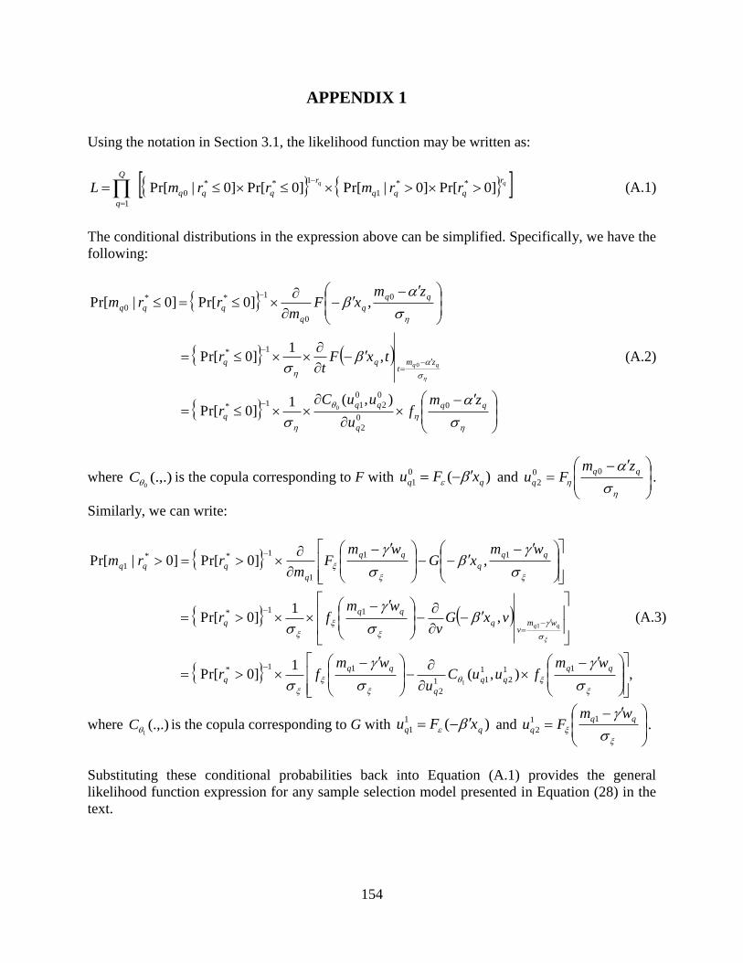
154
APPENDIX 1
Using the notation in Section 3.1, the likelihood function may be written as:
qq r
qqq
r
qqq
Q
q
rrmrrmL ]0Pr[]0|Pr[ ]0Pr[]0|Pr[ **
1
1**
0
1
(A.1)
The conditional distributions in the expression above can be simplified. Specifically, we have the
following:
q
q
zmt
q
q
qqq
zmf
u
uuCr
txFt
r
zmxF
mrrm
0
0
2
0
2
0
11*
1*
0
0
1**
0
),(1]0Pr[
,1
]0Pr[
,]0Pr[ ]0|Pr[
0
0 (A.2)
where (.,.)0
C is the copula corresponding to F with )(0
1 qq xFu and
q
zmFu
00
2 .
Similarly, we can write:
,),(1
]0Pr[
,1
]0Pr[
,]0Pr[ ]0|Pr[
11
2
1
11
2
11*
11*
11
1
1**
1
1
1
q
q
wmv
q
q
q
q
qqq
wmfuuC
u
wmfr
vxGv
wmfr
wmxG
wmF
mrrm
qq(A.3)
where (.,.)1
C is the copula corresponding to G with )(1
1 qq xFu and
q
wmFu
11
2 .
Substituting these conditional probabilities back into Equation (A.1) provides the general
likelihood function expression for any sample selection model presented in Equation (28) in the
text.
155
REFERENCES
Arentze, T.A., and H.J.P. Timmermans. (2005) Albatross Version 2: A Learning-Based
Transportation Oriented Simulation System. European Institute of Retailing and Services
Studies, Eindhoven, The Netherlands.
Armstrong, M., (2003). Copula Catalogue - Part 1: Bivariate Archimedean Copulas. Unpublished
Paper, Cerna, Available At http://www.Cerna.Ensmp.Fr/Documents/MA-
Copulacatalogue.Pdf
Beige, S., and K.W. Axhausen. (2006) Long-Term Mobility Decisions During The Life Course:
Experiences With A Retrospective Survey. Presented At The 11th International
Conference on Travel Behaviour Research, Kyoto, Japan, August, 2006.
Ben-Akiva, M., and Lerman, S. R. (1985). Discrete Choice Analysis: Theory and Application to
Travel Demand, Cambridge, Massachusetts: MIT Press.
Bento, A. M., M.L. Cropper, A.M. Mobarak, K. Vinha. (2005) The Impact of Urban Spatial
Structure on Travel Demand in The United States. Review of Economics and Statistics,
Vol. 87,, Pp. 466-478.
Bhat, C.R., (2005) A Multiple Discrete-Continuous Extreme Value Model: Formulation and
Application to Discretionary Time-Use Decisions, Transportation Research Part B, Vol.
39, No. 8, Pp. 679-707.
Bhat, C.R., (2008) The Multiple Discrete-Continuous Extreme Value (MDCEV) Model: Role of
Utility Function Parameters, Identification Considerations, and Model Extensions.
Transportation Research Part B, 42(3), Pp. 274-303.
Bhat, C.R. (2003) Simulation Estimation of Mixed Discrete Choice Models Using Randomized
and Scrambled Halton Sequences. Transportation Research Part B, Vol. 37, No. 9, Pp.
837-855.
Bhat, C.R. (2001) Quasi-Random Maximum Simulated Likelihood Estimation of The Mixed
Multinomial Logit Model. Transportation Research Part B, Vol. 35, Pp. 677-693.
Bhat, C.R., and F.S. Koppelman, (1993). A Conceptual Framework of Individual Activity
Program Generation, Transportation Research Part A, Vol. 27, pp. 433-446.
Bhat, C.R., and F.S. Koppelman (1999) A Retrospective and Prospective Survey of Time-Use
Research. Transportation 26(2), Pp. 119-139.
Bhat, C. R., and N. Eluru. (2009) A Copula-Based Approach to Accommodate Residential Self-
Selection Effects in Travel Behavior Modeling. Transportation Research Part B, Vol. 43,
No. 7, Pp. 749-765.
156
Bhat, C.R., Guo J.Y., (2007). A Comprehensive Analysis of Built Environment Characteristics
on Household Residential Choice and Auto Ownership Levels. Transportation Research
Part B 41(5), 506-526.
Bhat, C.R., J.Y. Guo, S. Srinivasan, and A. Sivakumar (2004), "Comprehensive Econometric
Microsimulator for Daily Activity-Travel Patterns," Transportation Research Record, Vol.
1894, pp. 57-66
Bhat, C. R., S. Sen, and N. Eluru (2009). The Impact of Demographics, Built Environment
Attributes, Vehicle Characteristics, and Gasoline Prices on Household Vehicle Holdings
and Use. Transportation Research Part B, Vol. 43, No. 1, Pp. 1-18.
Bhat, C.R., Sener, I.N., (2009). A Copula-Based Closed-Form Binary Logit Choice Model for
Accommodating Spatial Correlation Across Observational Units. Presented At 88th
Annual Meeting of the Transportation Research Board, Washington, D.C.
Bhat, C.R., S. Srinivasan, and S. Sen, (2006) A Joint Model for the Perfect and Imperfect
Substitute Goods Case: Application to Activity Time-Use Decisions, Transportation
Research Part B, Vol. 40, No. 10, Pp. 827-850.
Bierlaire, M., D. Bolduc and D. Mcfadden (2008) The Estimation of Generalized Extreme Value
Models From Choice-Based Samples, Transportation Research Part B, 42(4), Pp. 381-
394.
Boheim, R., and M.P. Taylor. (2002) Tied Down or Room to Move? Investigating Relationships
Between Housing Tenure, Employment Status and Residential Mobility in Britain. Scottish
Journal of Political Economy, Vol. 49, No. 4, 2002, Pp. 369-392.
Bourguignon, S., Carfantan, H., Idier, J., (2007). A Sparsity-Based Method For The Estimation
of Spectral Lines From Irregularly Sampled Data. IEEE Journal of Selected Topics in
Signal Processing 1(4), 575-585.
Bowman J, (1995) Activity Based Disaggregate Travel Demand Model System with Daily
Activity Schedules. Master of Science Thesis in Transportation, Massachusetts Institute of
Technology.
Bowman, J.L., and M. A. Bradley (2006) Upward Integration of Hierarchical Activity-Based
Models. Working Paper, Available at
http://www.Jbowman.Net/Papers/20060117%20Bowman%20and%20Bradley.Pdf
Boyer, B., Gibson, M., Loretan, M., (1999). Pitfalls in Tests for Changes in Correlation.
International Finance Discussion Paper 597, Board of Governors of the Federal Reserve
System.
Briesch, R. A., Chintagunta, P. K., Matzkin, R. L., (2002). Semiparametric Estimation of Brand
Choice Behavior. Journal of the American Statistical Association 97(460), 973-982.
157
Brownstone, D., and T. F. Golob (2009). The Impact of Residential Density on Vehicle Usage
and Energy Consumption. Journal of Urban Economics, Vol. 65, Pp. 91-98.
Cameron, A. C., Li, T., Trivedi, P., Zimmer, D., (2004). Modelling The Differences in Counted
Outcomes Using Bivariate Copula Models With Application to Mismeasured Counts. The
Econometrics Journal 7(2), 566-584.
Cao, X., P. L. Mokhtarian, and S. L. Handy, (2006) Neighborhood Design and Vehicle Type
Choice: Evidence From Northern California. Transportation Research Part D, Vol. 13,
No. 2, Pp. 133-145.
Cao, X., P. L. Mokhtarian, and S. L. Handy (2008). Examining the Impacts of Residential Self-
Selection on Travel Behavior: Methodologies and Empirical Findings. Research Report
No. CTS 08-24,. http://www.tc.umn.edu/~Cao/08-24WEB.pdf >.
Chen, C., H. Gong, and R. Paaswell. (2008) Role of the Built Environment on Mode Choice
Decisions: Additional Evidence on the Impact of Density. Transportation, Vol. 35, Pp.
285-299.
Cherubini, U., Luciano, E., Vecchiato, W., (2004). Copula Methods in Finance. John Wiley &
Sons, Hoboken, NJ.
Choo, S., and P. L. Mokhtarian (2004). What Type of Vehicle Do People Drive? The Role of
Attitude and Lifestyle in Influencing Vehicle Type Choice. Transportation Research Part
A, Vo. 38, No. 3, Pp. 201-222.
Clark, W.A.V., and Y. Huang (2003). The Life Course and Residential Mobility in British
Housing Markets. Environment and Planning A, Vol. 35, Pp. 323-339.
Clark, W.A.V., Y.Q. Huang, and S. Withers (2003). Does Commuting Distance Matter?
Commuting Tolerance and Residential Change. Regional Science and Urban Economics,
Vol. 33, No. 2, Pp. 199-221.
Clark, W.A.V., and J.L. Onaka (1983). Life Cycle and Housing Adjustment As Explanations of
Residential Mobility. Urban Studies, Vol. 20, Pp. 47-57.
Clayton, D. G., (1978). A Model for Association in Bivariate Life Tables and its Application in
Epidemiological Studies of Family Tendency in Chronic Disease Incidence. Biometrika
65(1), 141-151.
PB Consult (2005) The MORPC Travel Demand Model: Validation and Final Report. The Mid-
Ohio Regional Planning Commission, Columbus, Ohio.
Conway, D. A., (1979). Multivariate Distributions With Specified Marginals. Technical Report
#145, Department of Statistics, Stanford University.
158
Cosslett, S. R., (1983). Distribution-Free Maximum Likelihood Estimation of The Binary Choice
Model. Econometrica 51(3), 765-782.
Coupe, R.T., and B.S. Morgan (1981). Towards A Fuller Understanding of Residential Mobility:
A Case Study of Northampton, England. Environment and Planning A, Vol. 13, Pp. 201-
215.
Dieleman, F.M (2001). Modeling Residential Mobility: A Review of Recent Trends in Research.
Journal of Housing and the Built Environment, Vol. 16, Pp. 249-265.
Dube, J. P (2004). Multiple Discreteness and Product Differentiation: Demand for Carbonated
Soft Drinks. Marketing Science, Vol. 23, No. 1, 66-81.
Dubin, J. A., Mcfadden, D. L, (1984). An Econometric Analysis of Residential Electric
Appliance Holdings and Consumption. Econometrica 52(1), 345-362.
Eliasson, J., and L. Mattsson (2000). A Model For Integrated Analysis of Household Location
and Travel Choices. Transportation Research Part A, Vol. 34, No. 5, Pp. 375-394.
Eluru, N. and C.R. Bhat. A Joint Econometric Analysis of Seat Belt Use and Crash-Related
Injury Severity. Accident Analysis and Prevention, Vol. 39, No. 5, 2007, Pp. 1037-1049.
Eluru, N., A.R. Pinjari, J.Y. Guo, I.N. Sener, S. Srinivasan, R.B. Copperman, and C.R. Bhat
(2008), "Population Updating System Structures and Models Embedded in the
Comprehensive Econometric Microsimulator for Urban Systems," Transportation
Research Record, Vol. 2076, pp. 171-182
Embrechts, P., Mcneil, A. J., Straumann, D., (2002). Correlation and Dependence in Risk
Management: Properties and Pitfalls. in M. Dempster (Ed.) Risk Management: Value At
Risk and Beyond, Cambridge University Press, Cambridge, 176-223.
Ewing, R., and R. Cervero (2001). Travel and the Built Environment – Synthesis. in
Transportation Research Record: Journal of The Transportation Research Board, No.
1780, Transportation Research Board of The National Academies, Washington, D.C., Pp.
87-114.
Farlie, D. J. G., (1960). The Performance of Some Correlation Coefficients For A General
Bivariate Distribution. Biometrika 47(3-4), 307-323.
Feng Y., D. Fullerton, and L. Gan (2005). Vehicle Choices, Miles Driven and Pollution Policies.
NBER Working Paper Series, Working Paper 11553, National Bureau of Economic
Research, Washington, D.C..
Frank, M. J., (1979). on The Simultaneous Associativity of F(X, Y) and X + Y - F(X, Y).
Aequationes Mathematicae 19(1), 194-226.
159
Frees, E. W., Wang, P. (2005). Credibility Using Copulas. North American Actuarial Journal
9(2), 31-48.
Genest, C., Favre, A.-C., (2007). Everything You Always Wanted to Know About Copula
Modeling But Were Afraid to Ask. Journal of Hydrologic Engineering 12(4), 347-368.
Genest, C., Mackay, R. J., (1986). Copules Archimediennes Et Familles De Lois
Bidimensionnelles Dont Les Marges Sont Donnees. The Canadian Journal of Statistics
14(2), 145-159.
Genius, M., Strazzera, E., (2008). Applying The Copula Approach to Sample Selection
Modeling. Applied Economics 40(11), 1443-1455.
Goldberg, P (1998). The Effects of The Corporate Average Fuel Efficiency Standards in The US.
Journal of Industrial Economics, Vol. 46, No. 1, Pp. 1-33.
Greene, W.H (2000). Econometric Analysis (4th Edn). Prentice-Hall, Englewood Cliffs, New
Jersey.
Greene, W., (1981). Sample Selection Bias As A Specification Error: A Comment.
Econometrica 49(3), 795-798.
Greene, D.L., Schafer, A., (2003). Reducing Greenhouse Gas Emissions from U.S.
Transportation, PEW Center on Global Climate Change, May 2003, Arlington, VA
Grimaldi, S., Serinaldi, F., (2006). Asymmetric Copula in Multivariate Flood Frequency
Analysis. Advances in Water Resources 29(8), 1155-1167.
Gumbel, E. J., (1960). Bivariate Exponential Distributions. Journal of The American Statistical
Association 55(292), 698-707.
Guo, J.Y., and C.R. Bhat (2004) Modifiable Areal Units: Problem Or Perception in Modeling of
Residential Location Choice? Transportation Research Record 1898, Pp. 138-147.
Guo, J.Y., and C.R. Bhat (2007), "Population Synthesis for Microsimulating Travel
Behavior," Transportation Research Record, Vol. 2014, pp. 92-101
Handy, S (2005). Critical Assessment of The Literature on The Relationships Among
Transportation, Land Use, and Physical Activity. Prepared For The Transportation
Research Board and Institute of Medicine Committee on Physical Activity, Health,
Transportation, and Land Use. Washington, D.C., January 2005. Available At
http://Trb.Org/Downloads/Sr282papers/Sr282handy.Pdf.
160
Hay, J. W., (1980). Occupational Choice and Occupational Earnings: Selectivity Bias in A
Simultaneous Logit-OLS Model. Ph.D. Dissertation, Department of Economics, Yale
University.
Heckman, J. (1974) Shadow Prices, Market Wages and Labor Supply. Econometrica, 42(4), 679-
694.
Heckman, J. (1976) The Common Structure of Statistical Models of Truncation, Sample
Selection, and Limited Dependent Variables and A Simple Estimator For Such Models.
The Annals of Economic and Social Measurement, 5(4), 475-492.
Heckman, J. J., (1979) Sample Selection Bias as a Specification Error, Econometrica, 47(1),
153-161.
Heckman, J. J., (2001). Microdata, Heterogeneity and the Evaluation of Public Policy. Journal of
Political Economy 109(4), 673-748.
Heckman, J. J., Robb, R., (1985). Alternative Methods for Evaluating The Impact of
Interventions. in J. J. Heckman and B. Singer (Eds.), Longitudinal Analysis of Labor
Market Data, Cambridge University Press, New York, 156-245.
Heckman, J. J., Vytlacil, E. J., (2000). The Relationship Between Treatment Parameters Within
A Latent Variable Framework. Economics Letters 66(1), 33-39.
Heckman, J. J., Vytlacil, E. J., (2005). Structural Equations, Treatment Effects and Econometric
Policy Evaluation. Econometrica 73(3), 669-738.
Heckman, J. J., Tobias, J. L., Vytlacil, E. J., (2001). Four Parameters of Interest in the Evaluation
of Social Programs. Southern Economic Journal 68(2), 210-223.
Hendel, I (1999). Estimating Multiple-Discrete Choice Models: An Application to
Computerization Returns. Review of Economic Studies, Vol. 66, Pp. 423-446.
Hollingworth, B.J., and E.J. Miller (1996). Retrospective Interviewing and Its Application in
Study of Residential Mobility. in Transportation Research Record: Journal of The
Transportation Research Board, No. 1551, Transportation Research Board of The National
Academies, Washington, D.C., Pp. 74-81.
Huard, D., Evin, G., Favre, A.-C., (2006). Bayesian Copula Selection. Computational Statistics
& Data Analysis 51(2), 809-822.
Ichimura, H., (1993). Semiparametric Least Squares (SLS) and Weighted SLS Estimation of
Single-Index Models. Journal of Econometrics 58(1-2), 71-120.
Jara-Diaz, S.R., M. Munizaga, P. Greeven. and R. Guerra (2007) The Unified Expanded Goods-
Activities-Travel Model: Theory and Results. Paper Presented At The 11th World
Conference on Transport Research, Berkeley, June 24 – 28.
161
Joe, H., (1993). Parametric Families of Multivariate Distributions With Given Marginals.
Journal of Multivariate Analysis 46(2), 262-282.
Joe, H., (1997). Multivariate Models and Dependence Concepts. Chapman and Hall, London.
Junker, M., May, A., (2005). Measurement of Aggregate Risk With Copulas. The Econometrics
Journal 8(3), 428-454.
Kan, K (2007). Residential Mobility and Social Capital. Journal of Urban Economics, Vol. 61,
No. 3, Pp. 436-457.
Kim, J.H., F. Pagliara, and J. Preston (2005). The Intention to Move and Residential Location
Choice Behaviour. Urban Studies, Vol. 9, Pp. 1-16.
Kotz, S., Balakrishnan, N., Johnson, N. L., (2000). Continuous Multivariate Distributions, Vol.
1, Models and Applications, 2nd Edition. John Wiley & Sons, New York.
Kwerel, S. M., (1988). Frechet Bounds. in S. Kotz, N. L. Johnson (Eds.) Encyclopedia of
Statistical Sciences, Wiley & Sons, New York, 202-209.
Lee, L.-F., (1978). Unionism and Wage Rates: A Simultaneous Equation Model With Qualitative
and Limited Dependent Variables. International Economic Review 19(2), 415-433.
Lee, L.-F., (1982). Some Approaches to The Correction of Selectivity Bias. Review of Economic
Studies 49(3), 355-372.
Lee, L.-F., (1983). Generalized Econometric Models With Selectivity. Econometrica 51(2), 507-
512.
Leung, S. F., Yu, S., (2000). Collinearity and Two-Step Estimation of Sample Selection Models:
Problems, Origins, and Remedies. Computational Economics 15(3), 173-199.
Li, S.-M. (2004) Life Course and Residential Mobility in Beijing, China. Environment and
Planning A, Vol. 36, Pp. 27-43.
Lin, D-Y., N. Eluru, S.T. Waller, and C.R. Bhat (2008), "Integration of Activity-Based Modeling
and Dynamic Traffic Assignment," Transportation Research Record,Vol. 2076, pp. 52-61
Lu, X. L., Pas, E. I., (1999). Socio-Demographics, Activity Participation, and Travel Behavior.
Transportation Research Part A 33(1), 1-18.
Lund, H (2003). Testing The Claims of New Urbanism. Journal of The American Planning
Association, Vol. 69,No. 4, Pp. 414-429.
162
Maddala, G. S., (1983). Limited-Dependent and Qualitative Variables in Econometrics.
Cambridge University Press.
Mannering, F., and C. Winston (1985). A Dynamic Empirical Analysis of Household Vehicle
Ownership and Utilization. Rand Journal of Economics, Vol. 16, No. 2, Pp. 215-236.
Matzkin, R. L., (1992). Nonparametric and Distribution-Free Estimation of the Binary Choice
and The Threshold Crossing Models. Econometrica 60(2), 239-270.
Matzkin, R. L., (1993). Nonparametric Identification and Estimation of Polychotomous Choice
Models. Journal of Econometrics 58(1-2), 137-168.
Mcfadden, D (1978). Modelling the Choice of Residential Location. in Spatial Interaction
Theory and Planning Models, A. Karquist Et Al. (Eds.), North-Holland Press, Amsterdam.
Meester, S. G., Mackay, J., (1994). A Parametric Model For Cluster Correlated Categorical Data.
Biometrics 50(4), 954-963.
Meloni, I., L. Guala, and A. Loddo (2004) Time Allocation to Discretionary in Home, Out of
Home Activities and to Trips. Transportation, 31(1), Pp. 69-96.
Micocci, M., Masala, G., (2003). Pricing Pension Funds Guarantees Using A Copula Approach.
Presented At AFIR Colloquium, International Actuarial Association, Maastricht,
Netherlands.
Miller, E.J. and M.J. Roorda (2003) A Prototype Model of Activity Scheduling. Transportation
Research Record 1831, Pp. 114-121.
Mohammadian, A., and E. J. Miller (2003). Empirical Investigation of Household Vehicle Type
Choice Decisions. in Transportation Research Record: Journal of The Transportation
Research Board, No. 1854, Transportation Research Board of The National Academies,
Washington, D.C., Pp. 99-106.
Morgenstern, D., (1956). Einfache Beispiele Zweidimensionaler Verteilungen. Mitteilingsblatt
Fur Mathematische Statistik 8(3), 234-235.
Nelsen, R. B., (2006). An Introduction to Copulas (2nd Ed). Springer-Verlag, New York.
Pendyala, R.M., R. Kitamura, A. Kikuchi, T. Yamamoto, and S. Fujii (2005) FAMOS: The
Florida Activity Mobility Simulator. Transportation Research Record 1921, Pp. 123-130.
Pinjari, A.R., and C.R. Bhat (2009a) A Multiple Discrete-Continuous Nested Extreme Value
(MDCNEV) Model: Formulation and Application to Non-Worker Activity Time-Use and
Timing Behavior on Weekdays. Forthcoming, Transportation Research Part B.
163
Pinjari, A.R., and C.R. Bhat (2009b) An Efficient Forecasting Procedure For Kuhn-Tucker
Consumer Demand Model Systems. Technical Paper, Department of Civil &
Environmental Engineering, University of South Florida, August 2009.
Pinjari, A. R., C. R. Bhat, and D. A. Hensher (2009). Residential Self-Selection Effects in An
Activity Time-Use Behavior Model. Transportation Research Part B, Vol. 43, No. 7, Pp.
729-748.
Pinjari, A. R., Eluru, N., Bhat, C. R., Pendyala, R. M., Spissu, E., (2008). Joint Model of Choice
of Residential Neighborhood and Bicycle Ownership: Accounting For Self-Selection and
Unobserved Heterogeneity. Transportation Research Record 2082, 17-26.
Pinjari, A., N. Eluru, R. Copperman, I.N. Sener, J.Y. Guo, S. Srinivasan, and C.R. Bhat (2006)
Activity-Based Travel-Demand Analysis For Metropolitan Areas in Texas: CEMDAP
Models, Framework, Software Architecture and Application Results. Report 4080-8,
Prepared For The Texas Department of Transportation, October.
Pinjari, A.R., R.M. Pendyala, C.R. Bhat, and P.A. Waddell (2008). Modeling The Choice
Continuum: An Integrated Model of Residential Location, Auto Ownership, Bicycle
Ownership, and Commute Tour Mode Choice Decisions. Technical Paper, Department of
Civil, Architectural and Environmental Engineering, The University of Texas At Austin.
Polzin S.E., X. Chu and L. Toole-Holt, (2004) Forecasts of future vehicle miles of travel in the
United States, Transportation Research Record 1895 pp. 147–155
Prieger, J. E., (2002). A Flexible Parametric Selection Model For Non-Normal Data With
Application to Health Care Usage. Journal of Applied Econometrics 17(4), 367-392.
Pucher J., and J. Renne (2003), Socioeconomics of urban travel: evidence from the 2001
NHTS, Transportation Quarterly 57 (3), pp. 49–78.
Puhani, P. A., (2000). The Heckman Correction For Sample Selection and Its Critique. Journal
of Economic Surveys 14(1), 53-67.
Quinn, C., (2007). The Health-Economic Applications of Copulas: Methods in Applied
Econometric Research. Health, Econometrics and Data Group (HEDG) Working Paper
07/22, Department of Economics, University of York
Rossi, P.H (1995). Why Families Move: A Study in The Social Psychology of Urban Residential
Mobility. The Free Press, Glencoe, Illinois..
Roy, A. D., (1951). Some Thoughts on The Distribution of Earnings. Oxford Economic Papers,
New Series 3(2), 135-146.
164
Salon, D (2006). Cars and The City: An Investigation of Transportation and Residential Location
Choices in New York City. Dissertation, Department of Agricultural and Resource
Economics, University of California, Davis.
Salvini, P.A., and E.J. Miller (2005)). ILUTE: An Operational Prototype of A Comprehensive
Microsimulation Model of Urban Systems. Networks and Spatial Economics, Vol. 5, No. 2,
Pp. 217–234.
Schachter, J (2001). Why People Move: Exploring The March 2000 Current Population Survey.
U.S. Census Bureau, Washington, D.C., http://www.Census.Gov/Prod/2001pubs/P23-
204.Pdf
Schmidt, R., (2003). Credit Risk Modeling and Estimation via Elliptical Copulae. in G. Bol, G.
Nakhaeizadeh, S. T. Rachev, T. Ridder, and K.-H. Vollmer (Eds.) Credit Risk:
Measurement, Evaluation, and Management, 267-289, Physica-Verlag, Heidelberg.
Schmidt, T., (2007). Coping With Copulas in J. Rank (Ed.) Copulas - From Theory to
Application in Finance, 3-34, Risk Books, London.
Schrank, D., and Lomax, T., (2005). The 2005 urban mobility report. Texas Transportation
Institute, Texas A&M University
Schweizer, B., Sklar, A., (1983). Probabilistic Metric Spaces. North-Holland, New York.
Shay, E., and A. Khattak (2005). Automobile Ownership and Use in Neotraditional and
Conventional Neighborhoods. in Transportation Research Record: Journal of The
Transportation Research Board, No. 1902, Transportation Research Board of The National
Academies, Washington, D.C., Pp. 18-25.
Sklar, A., (1959). Fonctions De Répartition A N Dimensions Et Leurs Marges. Publications De
l'Institut De Statistique De L'Université De Paris, 8, 229-231.
Sklar, A., (1973). Random Variables, Joint Distribution Functions, and Copulas. Kybernetika 9,
449-460.
Smith, M. D., (2005). Using Copulas to Model Switching Regimes With An Application to Child
Labour. Economic Record 81(S1), S47-S57.
Song, Y., and G. J. Knaap (2003). New Urbanism and Housing Values: A Disaggregate
Assessment. Journal of Urban Economics, Vol. 54, Pp. 218-238.
Spissu, E., A. R. Pinjari, R. M. Pendyala, and C. R. Bhat (2009). A Copula-Based Joint
Multinomial Discrete-Continuous Model of Vehicle Type Choice and Miles of Travel.
Transportation, Vol. 36, No. 4, Pp. 403-422.
165
Train, K (1986). Qualitative Choice Analysis: Theory, Econometrics, and An Application to
Automobile Demand. MIT Press, Cambridge, MA.
Trivedi, P. K., and D. M. Zimmer (2007). Copula Modeling: An Introduction For Practitioners.
Foundations and Trends in Econometrics, Vol. 1, No. 1, Pp. 1-110.
U.S. Census Bureau (2005). Geographical Mobility Between 2003 and 2004. U.S. Census
Bureau, Washington, D.C., 2005. http://www.Census.Gov/Population/Pop-
Profile/Dynamic/Mobility.Pdf
Van Der Vlist, A., C. Gorter, P. Nijkamp, and P. Rietveld (2001). Residential Mobility and Local
Housing Market Differences. Tinbergen Institute Discussion Paper, University of
Amsterdam, The Netherlands.
Van Ommeren, J.N (1999). Job Moving, Residential Moving and Commuting: A Search
Perspective. Journal of Urban Economics, Vol. 46, Pp. 230-253.
Van Ommeren J.N., P. Rietveld, and P. Nijkamp (1998). Spatial Moving Behaviour of Two-
Earner Households. Journal of Regional Science, Vol. 38, No. 1, Pp. 23-46.
Vella, F., (1998). Estimating Models With Sample Selection Bias: A Survey. Journal of Human
Resources 33(1), 127-169.
Venter, G. G., (2001). Tails of Copulas. Presented At ASTIN Colloquium, International
Actuarial Association, Washington D.C.
Waddell, P., C.R. Bhat, N. Eluru, L. Wang, and R.M. Pendyala (2007). Modeling The
Interdependence in Household Residence and Workplace Choices. in Transportation
Research Record: Journal of The Transportation Research Board, No. 2003,
Transportation Research Board of The National Academies, Washington, D.C., Pp. 84-92.
Waddell, P., C.R. Bhat, E. Ruiter, S. Bekhor, M. Outwater, and E.L. Schroer (2001). Review of The
Literature and Operational Models: Final Report to The Puget Sound Regional Council on
Land Use and Travel Demand Forecasting Models.
Waddell, P., G.F. Ulfarsson, J.P. Franklin, and J. Lobb (2007). Incorporating Land Use in
Metropolitan Transportation Planning. Transportation Research Part A, Vol. 41, No. 5,
Pp. 382-410.
West, S (2004). Distributional Effects of Alternative Vehicle Pollution Control Policies. Journal
of Public Economics, Vol. 88, Pp. 735-757.
Xin Y., Karthik K., Ram P., Bhargava S., and P. Waddell (2009). A Methodology to Match
Distributions of Both Household and Person Attributes in the Generation of Synthetic
Populations. Presented at the 88th Annual Meetings of the Transportation Research Board
166
Yamamoto, T., R. Kitamura, and S. Kimura (1999). Competing-Risks-Duration Model of
Household Vehicle Transactions With Indicators of Changes in Explanatory Variables. in
Transportation Research Record: Journal of The Transportation Research Board, No.
1676, Transportation Research Board of The National Academies, Washington, D.C., Pp.
116-123.
Zimmer, D. M., Trivedi, P. K., (2006). Using Trivariate Copulas to Model Sample Selection and
Treatment Effects: Application to Family Health Care Demand. Journal of Business and
Economic Statistics 24(1), 63-76.
167
VITA
Naveen Eluru was born to his parents, Babu Rao and Swarajyam, in Tanuku, India. He went to
S.F.S High School, Tanuku. After completing high school at Gowtham Junior College,
Vijayawada, he entered Indian Institute of Technology Madras, India. He graduated successfully
from IIT Madras with a Bachelor‟s degree in Civil Engineering in the year 2004. In August 2004
he joined University of Texas Austin as a Graduate Research Assistant to pursue graduate studies
in Transportation Systems Engineering under the guidance of Dr. Chandra R. Bhat. He
completed his Masters of Science in Engineering in December 2005. Subsequently, he is
continuing for his Doctoral degree under the guidance of Dr. Bhat.
Permanent address: H.No.6-27, Rythupeta,
Nandigama, 521185, Andhra Pradesh, India
This dissertation was typed by the author.