cooperative advertising in a dynamic retail market … advertising in a dynamic retail ... duopoly...
TRANSCRIPT

Cooperative Advertising in a Dynamic Retail MarketDuopoly
Anshuman Chutani ∗, Suresh P. Sethi †
Abstract
Cooperative advertising is a key incentive offered by a manufacturer to influence re-tailers’ promotional decisions. We study cooperative advertising in a dynamic retailduopoly where a manufacturer sells his product through two competing retailers. Wemodel the problem as a Stackelberg differential game in which the manufacturer an-nounces his shares of advertising costs of the two retailers or his subsidy rates, and theretailers in response play a Nash differential game in choosing their optimal advertisingefforts over time. We obtain the feedback equilibrium solution consisting of the optimaladvertising policies of the retailers and manufacturer’s subsidy rates. We identify keydrivers that influence the optimal subsidy rates and in particular, obtain the conditionsunder which the manufacturer will support one or both of the retailers. We analyzeits impact on profits of channel members and the extent to which it can coordinatethe channel. We investigate the case of an anti-discriminatory act which restricts themanufacturer to offer equal subsidy rates to the two retailers. Finally, we discuss twoextensions: First, a retail oligopoly with any number of retailers, and second, the re-tail duopoly that also considers optimal wholesale and retail pricing decisions of themanufacturer and retailer, respectively.
Keywords: Cooperative advertising, Nash differential game, Stackelberg differential game,sales-advertising dynamics, Sethi model, feedback Stackelberg equilibrium, retail level com-petition, channel coordination, Robinson-Patman act.
∗Visiting Assistant Professor, School of Management, Binghamton University, State University of NewYork, PO Box 6000, Binghamton, NY, 13902e-mail: [email protected]†Charles & Nancy Davidson Distinguished Professor of Operations Management, School of Management,
Mail Station SM30, The University of Texas at Dallas, 800 W. Campbell Rd. Richardson, Texas 75080-3021e-mail: [email protected]

1 Introduction
Cooperative advertising is a common means by which a manufacturer incentivizes retailers
to advertise its product to increase its sales. In a typical arrangement, the manufacturer
contributes a percentage of a retailer’s advertising expenditures to promote the product. We
consider a marketing channel involving a manufacturer and two retailers. We model the
problem of the channel as a Stackelberg differential game in which the manufacturer acts as
the leader by announcing its subsidy rate to each of the two retailers, who act as followers
and play a Nash Differential game in order to obtain their optimal advertising efforts in
response to the support offered by the manufacturer.
Cooperative advertising is a fast increasing activity in retailing amounting to billions of
dollars a year. Nagler (2006) found that the total expenditure on cooperative advertising
in 2000 was estimated at $15 billion, compared with $900 million in 1970 and according to
some recent estimates, it was higher that $25 billion in 2007. Cooperative advertising can
be a significant part of the manufacturer’s expense according to Dant and Berger (1996),
and as many as 25-40% of local advertisements and promotions are cooperatively funded. In
addition, Dutta et al. (1995) report that the subsidy rates differ from industry to industry:
it is 88.38% for consumer convenience products, 69.85% for other consumer products, and
69.29% for industrial products.
Many researchers in the past have used static models to study cooperative advertising.
Berger (1972) modeled cooperative advertising in the form of a wholesale price discount
offered by the manufacturer to its retailer as an advertising allowance. He concluded that
both the manufacturer and the retailer can do better with cooperative advertising. Dant and
Berger (1996) extended the Berger model to incorporate demand uncertainty and considered
a scenario where the manufacturer and its retailer have a different opinion on anticipated
sales. Kali (1998) examined cooperative advertising subsidy with a threshold minimum ad-
vertised price by the retailer, and found that the channel can be coordinated in this case.
Huang et al. (2002) allowed for advertising by the manufacturer in addition to coopera-
1
tive advertising, and justified their static model by making a case for short-term effects of
promotion.
Jørgensen et al. (2000) formulated a dynamic model with cooperative advertising, as a
Stackelberg differential game between a manufacturer and a retailer with the manufacturer as
the leader. They considered short term as well as long term forms of advertising efforts made
by the retailer as well as the manufacturer. They showed that the manufacturer’s support
of both types of retailer advertising benefits both channel members more than support of
just one type, which in turn is more beneficial than no support at all. Jørgensen et al.
(2001) modified the above model by introducing decreasing marginal returns to goodwill
and studied two scenarios: a Nash game without advertising support and a Stackelberg
game with support from the manufacturer as the leader. Jørgensen et al. (2003) explored
the possibility of advertising cooperation even when the retailer’s promotional efforts may
erode the brand image. Karray and Zaccour (2005) extended the above model to consider
both the manufacturer’s national advertising and the retailer’s local promotional effort. All
of these papers use the Nerlove-Arrow (1962) model, in which goodwill increases linearly in
advertising and decreases linearly in goodwill, and there is no interacting term between sales
and advertising effort in the dynamics of sales.
He et al. (2009) solved a manufacturer-retailer Stackelberg game with cooperative ad-
vertising using the stochastic sales-advertising model proposed by Sethi (1983), in which the
effectiveness of advertising in increasing sales decreases as sales increase. The Sethi model
was validated empirically by Chintagunta and Jain (1995) and Naik et al. (2008). Despite
the presence of the interactive term involving sales and advertising, He et al. (2009) were
able to obtain a feedback Stackelberg solution for the retailer’s optimal advertising effort
and the manufacturer’s subsidy rate, and provided a condition for positive subsidy by the
manufacturer.
This paper extends the work of He et al. (2009) to allow for retail level competition
and provides useful managerial insights on the impact of this competition on the manufac-
2
turer’s decision. It contributes to the cooperative advertising literature in the following ways.
Firstly, most of the cooperative advertising literature uses a one manufacturer, one retailer
setting, with the exception of He et al. (2011), who study a retail duopoly. Their formula-
tion, however, is based on the Lanchester setting (see, for e.g., Little (1979)), in which the
two competitors split a given total market. We, on the other hand, use Erickson (2009)’s
duopolistic extension of the Sethi model, in which competitors could increase their shares of
a given total potential market at the same time. We formulate the model as a Stackelberg
differential game between the manufacturer as the leader and the retailers as the followers.
Furthermore, the two retailers competing for market share play a Nash game between them-
selves. While our model is considerably more complicated, we are still able to obtain, like
in He et al. (2009), a feedback equilibrium solution, sometimes explicitly and sometimes by
numerical means. We also explore the conditions under which the manufacturer supports
neither of the retailers, just one, or both. We consider the cases when the second retailer also
buys from the manufacturer and when he does not. When the second retailer does not buy
from the manufacturer, we are able to show the impact of the added retail level competition
on the manufacturer’s tendency to support the first retailer. Furthermore, we are able to
extend the above threshold conditions and the impact of retail level competition in explicit
form, to an extension considering an oligopoly of N identical retailers. Secondly, we inves-
tigate in greater detail the issue of supply chain coordination with cooperative advertising.
We study the extent to which the supply chain can be coordinated with cooperative adver-
tising, and its effect on the profits of all the parties in the supply chain. Finally, we look
into the case of anti-discrimination legislations (such as the Robinson-Patman Act against
price discrimination), under which the manufacturer is forced to offer equal subsidy rates
to the two retailers. We obtain feedback Stackelberg equilibrium in this case and compare
the optimal common subsidy rate with the two optimal subsidy rates without such an act.
We also investigate the impact of such legislations on profits of manufacturer, retailers and
overall supply chain, and subsequently, its role in coordinating the supply chain.
3
Papers →Issues addressed ↓
Ber
ger
(197
2)
Dan
t&
Ber
ger
(199
6)
Kal
i(1
998)
Huan
get
al.
(200
2)
Jør
gense
net
al.
(200
0)
Jør
gense
net
al.
(200
1)
Jør
gense
net
al.
(200
3)
Kar
ray
&Z
acco
ur
(200
5)
He
etal
.(2
009)
He
etal
.(2
011)
This
pap
er
Dynamic model X X X X X X XAdvertising interacting with sales X XStochastic demand X X XPricing decisions X X X XFeedback strategy X X X X X X XRetail level competition X X XChannel performance & coordination X X X X X X XAnti-discrimination legislation X
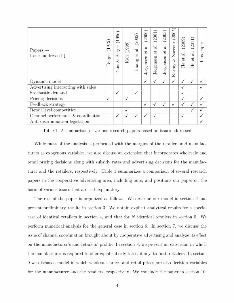
Table 1: A comparison of various research papers based on issues addressed
While most of the analysis is performed with the margins of the retailers and manufac-
turers as exogenous variables, we also discuss an extension that incorporates wholesale and
retail pricing decisions along with subsidy rates and advertising decisions for the manufac-
turer and the retailers, respectively. Table 1 summarizes a comparison of several research
papers in the cooperative advertising area, including ours, and positions our paper on the
basis of various issues that are self-explanatory.
The rest of the paper is organized as follows. We describe our model in section 2 and
present preliminary results in section 3. We obtain explicit analytical results for a special
case of identical retailers in section 4, and that for N identical retailers in section 5. We
perform numerical analysis for the general case in section 6. In section 7, we discuss the
issue of channel coordination brought about by cooperative advertising and analyze its effect
on the manufacturer’s and retailers’ profits. In section 8, we present an extension in which
the manufacturer is required to offer equal subsidy rates, if any, to both retailers. In section
9 we discuss a model in which wholesale prices and retail prices are also decision variables
for the manufacturer and the retailers, respectively. We conclude the paper in section 10.
4
Proofs of some of the results are relegated to the appendices of the paper. In Appendix D,
we discuss uniqueness of the optimal solution obtained in our analysis.
2 The model
We consider a dynamic market channel where a manufacturer sells its product through one
or both of two independent and competing retailers, labeled 1 and 2. The manufacturer may
choose to subsidize the advertising expenditures of the retailers. The subsidy, expressed as
a fraction of a retailer’s total advertising expenditure, is referred to as the manufacturer’s
subsidy rate for that retailer. We use the following notation in the paper:
t Time t ∈ [0,∞),
i Indicates retailer i, i = 1,2, when used as a subscript,
xi(t) ∈ [0, 1] Retailer i ’s proportional market share,
ui(t) Retailer i ’s advertising effort rate at time t,
θi(t) ≥ 0 Manufacturer’s subsidy rate for retailer i at time t ,
ρi > 0 Advertising effectiveness parameter of retailer i ,
δi ≥ 0 Market share decay parameter of retailer i ,
r > 0 Discount rate of the manufacturer and the retailers,
mi ≥ 0 Gross margin of retailer i ,
Mi ≥ 0 Gross margin of the manufacturer from retailer i ,
Vi, Vm Value functions of retailer i and of the manufacturer, respectively,
V Value function of the integrated channel;
also Vixj = ∂Vi/∂xj, i = 1, 2, j = 1, 2, and Vmxi = ∂Vm/∂xi and Vxi = ∂V/∂xi, i = 1, 2.
The state of the system is represented by the market share vector (x1, x2), so that the
5

state at time t is (x1(t), x2(t)). The sequence of events is as follows. First, the manufacturer
announces the subsidy rate θi(t) for retailer i, i = 1, 2, t ≥ 0. In response, the retailers
choose their respective advertising efforts u1(t) and u2(t) in order to compete for market
share. This situation is modeled as a Stackelberg game between the manufacturer as the
leader and the retailers as followers and a Nash differential game between the retailers; see
Fig. 1. The solution concept we employ is that of a feedback Stackelberg equilibrium. The
Figure 1: Sequence of Events
cost of advertising is assumed to be quadratic in the advertising effort, signifying a marginal
diminishing effect of advertising. Given the subsidy rates θi, the retailer i’s advertising
expenditure is (1−θi)u2i . The total advertising expenditure for the manufacturer is θ1u21+θ2u
22.
The quadratic cost function is common in the literature (see, e.g., Deal (1979), Chintagunta
and Jain (1992), Jorgensen et al. (2000), Prasad and Sethi (2004), Erickson (2009), and He
et al. (2009)).
To model the effect of advertising on sales over time, we use an oligopolistic extension of
the Sethi (1983) model, proposed by Erickson (2009). This extension is different from the
duopolistic extensions of the Sethi model studied by Sorger (1989), Prasad and Sethi (2004,
2009), and He et al. (2011), where the competitors split a given total market. Here, a gain
in the market share of one retailer comes from an equal loss of the market share of the other.
In contrast, the Erickson extension permits even a simultaneous increase of the retailers’
shares of a given total market potential. Moreover, Erickson (2009) used his extension to
study the competition between Anheuser-Busch, SABMiller, and Molson Coors in the beer
6
industry.
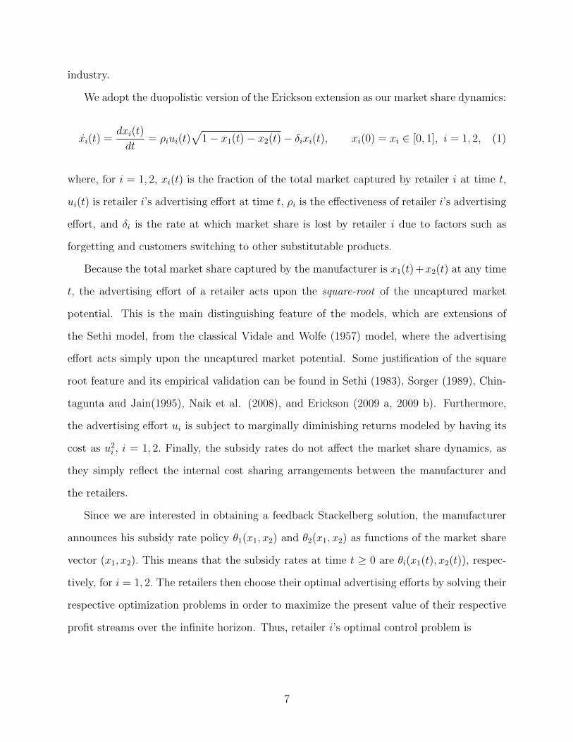
We adopt the duopolistic version of the Erickson extension as our market share dynamics:
xi(t) =dxi(t)
dt= ρiui(t)
√1− x1(t)− x2(t)− δixi(t), xi(0) = xi ∈ [0, 1], i = 1, 2, (1)
where, for i = 1, 2, xi(t) is the fraction of the total market captured by retailer i at time t,
ui(t) is retailer i’s advertising effort at time t, ρi is the effectiveness of retailer i’s advertising
effort, and δi is the rate at which market share is lost by retailer i due to factors such as
forgetting and customers switching to other substitutable products.
Because the total market share captured by the manufacturer is x1(t)+x2(t) at any time
t, the advertising effort of a retailer acts upon the square-root of the uncaptured market
potential. This is the main distinguishing feature of the models, which are extensions of
the Sethi model, from the classical Vidale and Wolfe (1957) model, where the advertising
effort acts simply upon the uncaptured market potential. Some justification of the square
root feature and its empirical validation can be found in Sethi (1983), Sorger (1989), Chin-
tagunta and Jain(1995), Naik et al. (2008), and Erickson (2009 a, 2009 b). Furthermore,
the advertising effort ui is subject to marginally diminishing returns modeled by having its
cost as u2i , i = 1, 2. Finally, the subsidy rates do not affect the market share dynamics, as
they simply reflect the internal cost sharing arrangements between the manufacturer and
the retailers.
Since we are interested in obtaining a feedback Stackelberg solution, the manufacturer
announces his subsidy rate policy θ1(x1, x2) and θ2(x1, x2) as functions of the market share
vector (x1, x2). This means that the subsidy rates at time t ≥ 0 are θi(x1(t), x2(t)), respec-
tively, for i = 1, 2. The retailers then choose their optimal advertising efforts by solving their
respective optimization problems in order to maximize the present value of their respective
profit streams over the infinite horizon. Thus, retailer i’s optimal control problem is
7

Vi(x1, x2) = maxui(t)≥0, t≥0
∫ ∞0
e−rt(mixi(t)− (1− θi(x1(t), x2(t)))u2i (t))dt, i = 1, 2, (2)
subject to (1), where we stress that x1 and x2 are initial conditions, which can be any given
values satisfying x1 ≥ 0, x2 ≥ 0 and x1 + x2 ≤ 1. Since retailer i’s problem is an infinite
horizon optimal control problem, we can define Vi(x1, x2) as his so-called value function. In
other words, Vi(x1, x2) also denotes the optimal value of the objective function of retailer
i at a time t ≥ 0, so long as x1(t) = x1 and x2(t) = x2 at that time. It should also
be mentioned that the problem (1)-(2) is a Nash differential game, whose solution will
give retailer i’s feedback advertising effort, expressed with a slight abuse of notation as
ui(x1, x2 | θ1(x1, x2), θ2(x1, x2)), respectively, for i = 1, 2.
The manufacturer anticipates the retailers’ optimal responses and incorporates these into
his optimal control problem, which is also a stationary infinite horizon problem. Thus, the
manufacturer’s problem is given by
Vm(x1, x2) = max0≤θ1(t)≤1, 0≤θ2(t)≤1, t≥0
∫ ∞0
e−rt{M1x1(t) +M2x2(t)
− θ1(t) [u1 (x1(t), x2(t) | θ1(t), θ2(t))]2 − θ2(t) [u2 (x1(t), x2(t) | θ1(t), θ2(t))]2}dt, (3)
subject to for i = 1, 2,
xi(t) = ρiui(x1(t), x2(t) | θ1(t), θ2(t))√
1− x1(t)− x2(t)− δixi(t), xi(0) = xi ∈ [0, 1]. (4)
Here, with an abuse of notation, θ1(t) and θ2(t) denote the subsidy rates at time t ≥ 0
to be obtained. Solution of the control problem (3)-(4) yields the optimal subsidy pol-
icy in feedback form expressed as θ∗i (x1, x2), i = 1, 2. Furthermore, we can express re-
tailer i’s feedback advertising policy, with an abuse of notation, as u∗i (x1, x2) = u∗i (x1, x2 |
θ∗1(x1, x2), θ∗2(x1, x2)), i = 1, 2.
8
The policies θ∗i (x1, x2) and u∗i (x1, x2), i = 1, 2, constitute a feedback Stackelberg equilib-
rium of the problem(1)-(4), which is time consistent, as opposed to an open-loop Stackelberg
equilibrium, which, in general, is not. Substituting these policies into the state equations in
(1) yields the market share process (x∗1(t), x∗2(t)), t ≥ 0, and the respective decisions, with
notational abuses, as θ∗i (t) = θ∗i (x∗1(t), x
∗2(t)) and u∗i (t) = u∗i (x
∗1(t), x
∗2(t)), t ≥ 0, i = 1, 2.
3 Preliminary results
We first solve the problem of retailer i to find the optimal advertising policy u∗i (x1, x2 |
θ1(x1, x2), θ2(x1, x2)), given the subsidy policies θ1(x1, x2) and θ2(x1, x2) announced by the
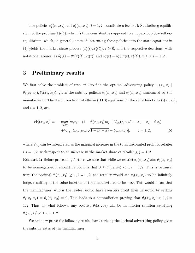
manufacturer. The Hamilton-Jacobi-Bellman (HJB) equations for the value functions Vi(x1, x2),
and i = 1, 2, are
rVi(x1, x2) = maxui≥0
[mixi − (1− θi(x1, x2))u2i + Vixi(ρiui√
1− x1 − x2 − δixi)
+Vix3−i(ρ3−iu3−i√
1− x1 − x2 − δ3−ix3−i)], i = 1, 2, (5)
where Vixj can be interpreted as the marginal increase in the total discounted profit of retailer
i, i = 1, 2, with respect to an increase in the market share of retailer j, j = 1, 2.
Remark 1: Before proceeding further, we note that while we restrict θ1(x1, x2) and θ2(x1, x2)
to be nonnegative, it should be obvious that 0 ≤ θi(x1, x2) < 1, i = 1, 2. This is because,
were the optimal θi(x1, x2) ≥ 1, i = 1, 2, the retailer would set ui(x1, x2) to be infinitely
large, resulting in the value function of the manufacturer to be −∞. This would mean that
the manufacturer, who is the leader, would have even less profit than he would by setting
θ1(x1, x2) = θ2(x1, x2) = 0. This leads to a contradiction proving that θi(x1, x2) < 1, i =
1, 2. Thus, in what follows, any positive θi(x1, x2) will be an interior solution satisfying
θi(x1, x2) < 1, i = 1, 2.
We can now prove the following result characterizing the optimal advertising policy given
the subsidy rates of the manufacturer.
9
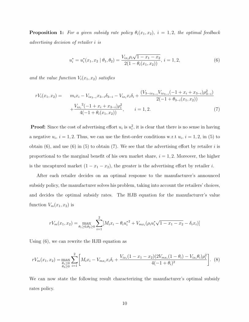
Proposition 1: For a given subsidy rate policy θi(x1, x2), i = 1, 2, the optimal feedback
advertising decision of retailer i is
u∗i = u∗i (x1, x2 | θ1, θ2) =Vixiρi
√1− x1 − x2
2(1− θi(x1, x2)), i = 1, 2, (6)
and the value function Vi(x1, x2) satisfies
rVi(x1, x2) = mixi − Vix3−ix3−iδ3−i − Vixixiδi +(V3−ix3−iVix3−i(−1 + xi + x3−i)ρ
23−i)
2(−1 + θ3−i(x1, x2))
+Vixi
2(−1 + xi + x3−i)ρ2i
4(−1 + θi(x1, x2)), i = 1, 2. (7)
Proof: Since the cost of advertising effort ui is u2i , it is clear that there is no sense in having
a negative ui, i = 1, 2. Thus, we can use the first-order conditions w.r.t ui, i = 1, 2, in (5) to
obtain (6), and use (6) in (5) to obtain (7). We see that the advertising effort by retailer i is
proportional to the marginal benefit of his own market share, i = 1, 2. Moreover, the higher
is the uncaptured market (1− x1 − x2), the greater is the advertising effort by retailer i.
After each retailer decides on an optimal response to the manufacturer’s announced
subsidy policy, the manufacturer solves his problem, taking into account the retailers’ choices,
and decides the optimal subsidy rates. The HJB equation for the manufacturer’s value
function Vm(x1, x2) is
rVm(x1, x2) = maxθ1≥0,θ2≥0
2∑i=1
[Mixi − θiu∗i2 + Vmxi(ρiu
∗i
√1− x1 − x2 − δixi)]
Using (6), we can rewrite the HJB equation as
rVm(x1, x2) = maxθ1≥0θ2≥0
2∑i=1
[Mixi − Vmxixiδi +
Vixi(1− x1 − x2)(2Vmxi(1− θi)− Vixiθi)ρ2i4(−1 + θi)2
]. (8)
We can now state the following result characterizing the manufacturer’s optimal subsidy
rates policy.
10
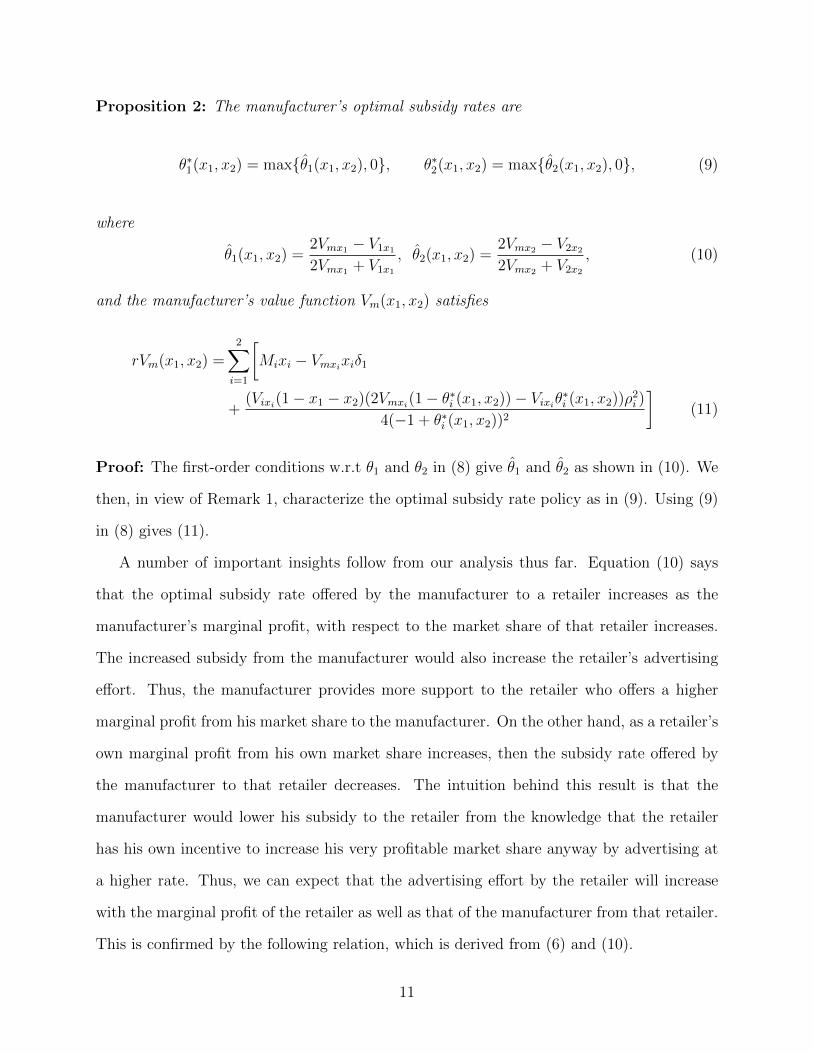
Proposition 2: The manufacturer’s optimal subsidy rates are
θ∗1(x1, x2) = max{θ1(x1, x2), 0}, θ∗2(x1, x2) = max{θ2(x1, x2), 0}, (9)
where
θ1(x1, x2) =2Vmx1 − V1x12Vmx1 + V1x1
, θ2(x1, x2) =2Vmx2 − V2x22Vmx2 + V2x2
, (10)
and the manufacturer’s value function Vm(x1, x2) satisfies
rVm(x1, x2) =2∑i=1
[Mixi − Vmxixiδ1
+(Vixi(1− x1 − x2)(2Vmxi(1− θ∗i (x1, x2))− Vixiθ∗i (x1, x2))ρ2i )
4(−1 + θ∗i (x1, x2))2
](11)
Proof: The first-order conditions w.r.t θ1 and θ2 in (8) give θ1 and θ2 as shown in (10). We
then, in view of Remark 1, characterize the optimal subsidy rate policy as in (9). Using (9)
in (8) gives (11).
A number of important insights follow from our analysis thus far. Equation (10) says
that the optimal subsidy rate offered by the manufacturer to a retailer increases as the
manufacturer’s marginal profit, with respect to the market share of that retailer increases.
The increased subsidy from the manufacturer would also increase the retailer’s advertising
effort. Thus, the manufacturer provides more support to the retailer who offers a higher
marginal profit from his market share to the manufacturer. On the other hand, as a retailer’s
own marginal profit from his own market share increases, then the subsidy rate offered by
the manufacturer to that retailer decreases. The intuition behind this result is that the
manufacturer would lower his subsidy to the retailer from the knowledge that the retailer
has his own incentive to increase his very profitable market share anyway by advertising at
a higher rate. Thus, we can expect that the advertising effort by the retailer will increase
with the marginal profit of the retailer as well as that of the manufacturer from that retailer.
This is confirmed by the following relation, which is derived from (6) and (10).
11
u∗i (x1, x2) =ρi(2Vmxi + Vixi)
√1− x1 − x2
4.
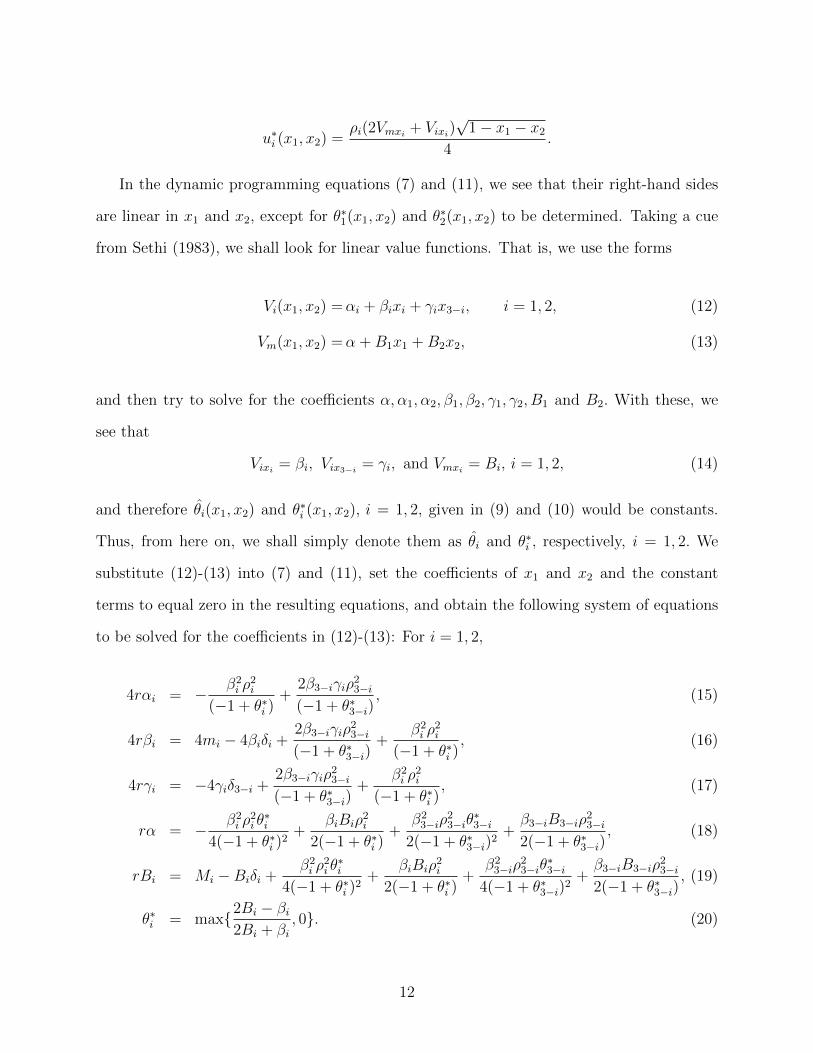
In the dynamic programming equations (7) and (11), we see that their right-hand sides
are linear in x1 and x2, except for θ∗1(x1, x2) and θ∗2(x1, x2) to be determined. Taking a cue
from Sethi (1983), we shall look for linear value functions. That is, we use the forms
Vi(x1, x2) =αi + βixi + γix3−i, i = 1, 2, (12)
Vm(x1, x2) =α +B1x1 +B2x2, (13)
and then try to solve for the coefficients α, α1, α2, β1, β2, γ1, γ2, B1 and B2. With these, we
see that
Vixi = βi, Vix3−i = γi, and Vmxi = Bi, i = 1, 2, (14)
and therefore θi(x1, x2) and θ∗i (x1, x2), i = 1, 2, given in (9) and (10) would be constants.
Thus, from here on, we shall simply denote them as θi and θ∗i , respectively, i = 1, 2. We
substitute (12)-(13) into (7) and (11), set the coefficients of x1 and x2 and the constant
terms to equal zero in the resulting equations, and obtain the following system of equations
to be solved for the coefficients in (12)-(13): For i = 1, 2,
4rαi = − β2i ρ
2i
(−1 + θ∗i )+
2β3−iγiρ23−i
(−1 + θ∗3−i), (15)
4rβi = 4mi − 4βiδi +2β3−iγiρ
23−i
(−1 + θ∗3−i)+
β2i ρ
2i
(−1 + θ∗i ), (16)
4rγi = −4γiδ3−i +2β3−iγiρ
23−i
(−1 + θ∗3−i)+
β2i ρ
2i
(−1 + θ∗i ), (17)
rα = − β2i ρ
2i θ∗i
4(−1 + θ∗i )2
+βiBiρ
2i
2(−1 + θ∗i )+
β23−iρ
23−iθ
∗3−i
2(−1 + θ∗3−i)2
+β3−iB3−iρ
23−i
2(−1 + θ∗3−i), (18)
rBi = Mi −Biδi +β2i ρ
2i θ∗i
4(−1 + θ∗i )2
+βiBiρ
2i
2(−1 + θ∗i )+
β23−iρ
23−iθ
∗3−i
4(−1 + θ∗3−i)2
+β3−iB3−iρ
23−i
2(−1 + θ∗3−i), (19)
θ∗i = max{2Bi − βi2Bi + βi
, 0}. (20)
12
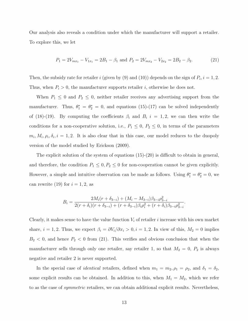
Our analysis also reveals a condition under which the manufacturer will support a retailer.
To explore this, we let
P1 = 2Vmx1 − V1x1 = 2B1 − β1 and P2 = 2Vmx2 − V2x2 = 2B2 − β2. (21)
Then, the subsidy rate for retailer i (given by (9) and (10)) depends on the sign of Pi, i = 1, 2.
Thus, when Pi > 0, the manufacturer supports retailer i, otherwise he does not.
When P1 ≤ 0 and P2 ≤ 0, neither retailer receives any advertising support from the
manufacturer. Thus, θ∗1 = θ∗2 = 0, and equations (15)-(17) can be solved independently
of (18)-(19). By computing the coefficients βi and Bi i = 1, 2, we can then write the
conditions for a non-cooperative solution, i.e., P1 ≤ 0, P2 ≤ 0, in terms of the parameters
mi,Mi, ρi, δi, i = 1, 2. It is also clear that in this case, our model reduces to the duopoly
version of the model studied by Erickson (2009).
The explicit solution of the system of equations (15)-(20) is difficult to obtain in general,
and therefore, the condition P1 ≤ 0, P2 ≤ 0 for non-cooperation cannot be given explicitly.
However, a simple and intuitive observation can be made as follows. Using θ∗1 = θ∗2 = 0, we
can rewrite (19) for i = 1, 2, as
Bi =2Mi(r + δ3−i) + (Mi −M3−i)β3−iρ
23−i
2(r + δi)(r + δ3−i) + (r + δ3−i)βiρ2i + (r + δi)β3−iρ23−i.
Clearly, it makes sense to have the value function Vi of retailer i increase with his own market
share, i = 1, 2. Thus, we expect βi = ∂Vi/∂xi > 0, i = 1, 2. In view of this, M2 = 0 implies
B2 < 0, and hence P2 < 0 from (21). This verifies and obvious conclusion that when the
manufacturer sells through only one retailer, say retailer 1, so that M2 = 0, P2 is always
negative and retailer 2 is never supported.
In the special case of identical retailers, defined when m1 = m2, ρ1 = ρ2, and δ1 = δ2,
some explicit results can be obtained. In addition to this, when M1 = M2, which we refer
to as the case of symmetric retailers, we can obtain additional explicit results. Nevertheless,
13
even in the general case, it is easy to solve the system numerically.
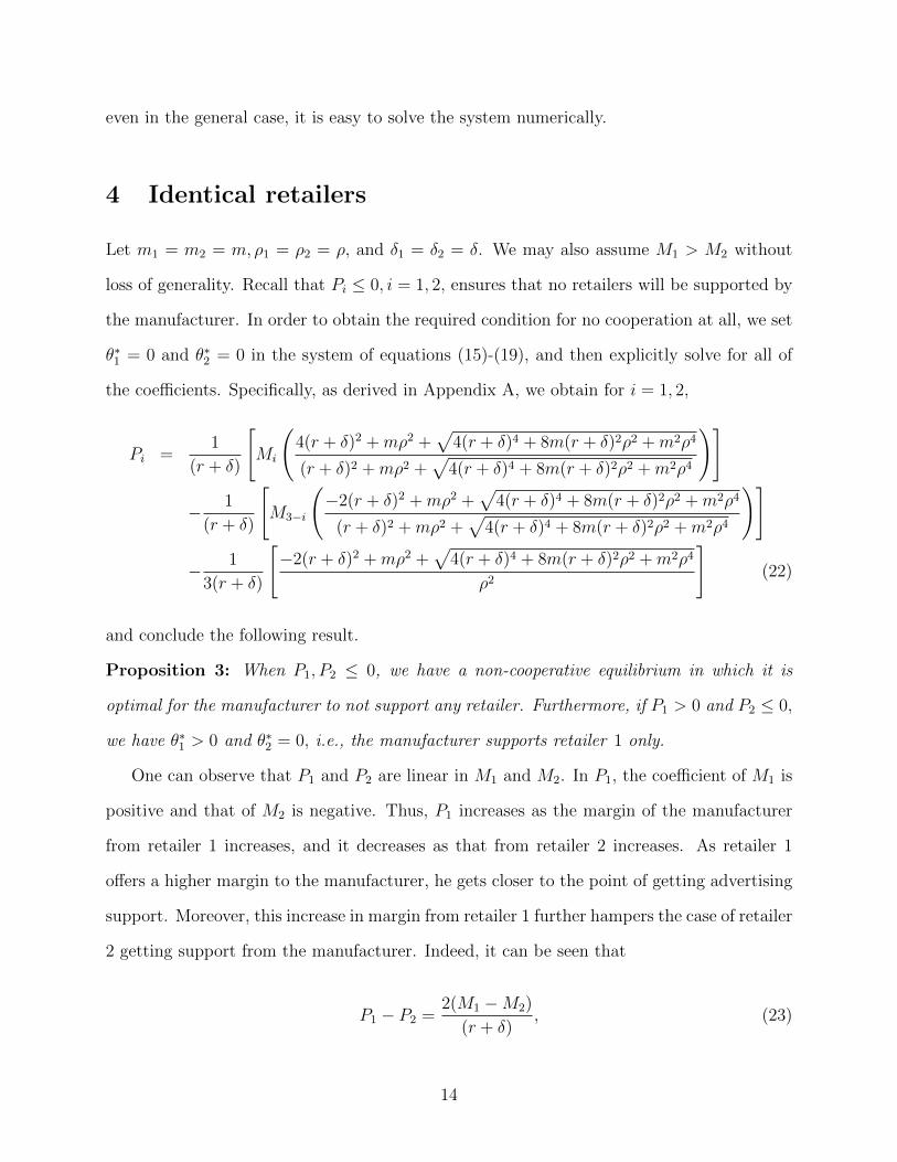
4 Identical retailers
Let m1 = m2 = m, ρ1 = ρ2 = ρ, and δ1 = δ2 = δ. We may also assume M1 > M2 without
loss of generality. Recall that Pi ≤ 0, i = 1, 2, ensures that no retailers will be supported by
the manufacturer. In order to obtain the required condition for no cooperation at all, we set
θ∗1 = 0 and θ∗2 = 0 in the system of equations (15)-(19), and then explicitly solve for all of
the coefficients. Specifically, as derived in Appendix A, we obtain for i = 1, 2,
Pi =1
(r + δ)
[Mi
(4(r + δ)2 +mρ2 +
√4(r + δ)4 + 8m(r + δ)2ρ2 +m2ρ4
(r + δ)2 +mρ2 +√
4(r + δ)4 + 8m(r + δ)2ρ2 +m2ρ4
)]
− 1
(r + δ)
[M3−i
(−2(r + δ)2 +mρ2 +
√4(r + δ)4 + 8m(r + δ)2ρ2 +m2ρ4
(r + δ)2 +mρ2 +√
4(r + δ)4 + 8m(r + δ)2ρ2 +m2ρ4
)]
− 1
3(r + δ)
[−2(r + δ)2 +mρ2 +
√4(r + δ)4 + 8m(r + δ)2ρ2 +m2ρ4
ρ2
](22)
and conclude the following result.
Proposition 3: When P1, P2 ≤ 0, we have a non-cooperative equilibrium in which it is
optimal for the manufacturer to not support any retailer. Furthermore, if P1 > 0 and P2 ≤ 0,
we have θ∗1 > 0 and θ∗2 = 0, i.e., the manufacturer supports retailer 1 only.
One can observe that P1 and P2 are linear in M1 and M2. In P1, the coefficient of M1 is
positive and that of M2 is negative. Thus, P1 increases as the margin of the manufacturer
from retailer 1 increases, and it decreases as that from retailer 2 increases. As retailer 1
offers a higher margin to the manufacturer, he gets closer to the point of getting advertising
support. Moreover, this increase in margin from retailer 1 further hampers the case of retailer
2 getting support from the manufacturer. Indeed, it can be seen that
P1 − P2 =2(M1 −M2)
(r + δ), (23)
14
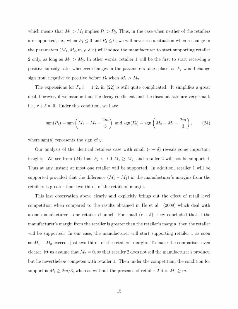
which means that M1 > M2 implies P1 > P2. Thus, in the case when neither of the retailers
are supported, i.e., when P1 ≤ 0 and P2 ≤ 0, we will never see a situation when a change in
the parameters (M1,M2,m, ρ, δ, r) will induce the manufacturer to start supporting retailer
2 only, as long as M1 > M2. In other words, retailer 1 will be the first to start receiving a
positive subsidy rate, whenever changes in the parameters takes place, as P1 would change
sign from negative to positive before P2 when M1 > M2.
The expressions for Pi, i = 1, 2, in (22) is still quite complicated. It simplifies a great
deal, however, if we assume that the decay coefficient and the discount rate are very small,
i.e., r + δ ≈ 0. Under this condition, we have
sgn(P1) = sgn
(M1 −M2 −
2m
3
)and sgn(P2) = sgn
(M2 −M1 −
2m
3
), (24)
where sgn(y) represents the sign of y.
Our analysis of the identical retailers case with small (r + δ) reveals some important
insights. We see from (24) that P2 < 0 if M1 ≥ M2, and retailer 2 will not be supported.
Thus at any instant at most one retailer will be supported. In addition, retailer 1 will be
supported provided that the difference (M1 −M2) in the manufacturer’s margins from the
retailers is greater than two-thirds of the retailers’ margin.
This last observation above clearly and explicitly brings out the effect of retail level
competition when compared to the results obtained in He et al. (2009) which deal with
a one manufacturer - one retailer channel. For small (r + δ), they concluded that if the
manufacturer’s margin from the retailer is greater than the retailer’s margin, then the retailer
will be supported. In our case, the manufacturer will start supporting retailer 1 as soon
as M1 −M2 exceeds just two-thirds of the retailers’ margin. To make the comparison even
clearer, let us assume that M2 = 0, so that retailer 2 does not sell the manufacturer’s product,
but he nevertheless competes with retailer 1. Then under the competition, the condition for
support is M1 ≥ 2m/3, whereas without the presence of retailer 2 it is M1 ≥ m.
15
4.1 Symmetric Retailers (M1 = M2 = M)
When M1 = M2 = M in addition to the retailers being identical, (22) reduces to
P1 = P2 =6M(r + δ)
(r + δ)2 +mρ2 +√
4(r + δ)4 + 8mρ2(r + δ)2 +m2ρ4
−−2(r + δ)2 +mρ2 +
√4(r + δ)4 + 8mρ2(r + δ)2 +m2ρ4
3(r + δ)ρ2.
We can see from the above expression that P1 and P2 would quickly approach a negative
value as (r+ δ) approaches 0, in fact when (r+ δ) ≈ 0, it approaches −∞. This can also be
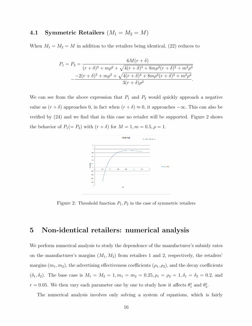
verified by (24) and we find that in this case no retailer will be supported. Figure 2 shows
the behavior of P1(= P2) with (r + δ) for M = 1,m = 0.5, ρ = 1.
Figure 2: Threshold function P1, P2 in the case of symmetric retailers
5 Non-identical retailers: numerical analysis
We perform numerical analysis to study the dependence of the manufacturer’s subsidy rates
on the manufacturer’s margins (M1,M2) from retailers 1 and 2, respectively, the retailers’
margins (m1,m2), the advertising effectiveness coefficients (ρ1, ρ2), and the decay coefficients
(δ1, δ2). The base case is M1 = M2 = 1,m1 = m2 = 0.25, ρ1 = ρ2 = 1, δ1 = δ2 = 0.2, and
r = 0.05. We then vary each parameter one by one to study how it affects θ∗1 and θ∗2.
The numerical analysis involves only solving a system of equations, which is fairly
16
straightforward to carry out. In all instances, we find a unique solution to the system.
For the case of symmetric retailers, we prove the uniqueness in Appendix D. In what follows,
we describe the results obtained from the numerical analysis.
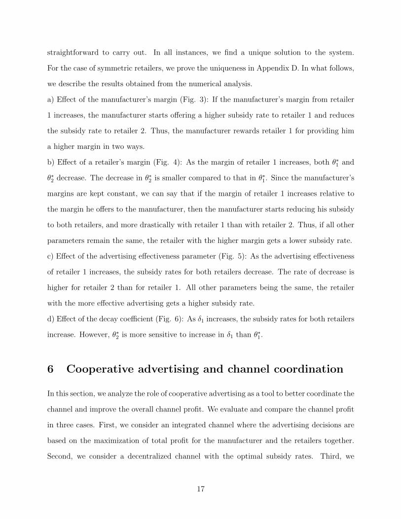
a) Effect of the manufacturer’s margin (Fig. 3): If the manufacturer’s margin from retailer
1 increases, the manufacturer starts offering a higher subsidy rate to retailer 1 and reduces
the subsidy rate to retailer 2. Thus, the manufacturer rewards retailer 1 for providing him
a higher margin in two ways.
b) Effect of a retailer’s margin (Fig. 4): As the margin of retailer 1 increases, both θ∗1 and
θ∗2 decrease. The decrease in θ∗2 is smaller compared to that in θ∗1. Since the manufacturer’s
margins are kept constant, we can say that if the margin of retailer 1 increases relative to
the margin he offers to the manufacturer, then the manufacturer starts reducing his subsidy
to both retailers, and more drastically with retailer 1 than with retailer 2. Thus, if all other
parameters remain the same, the retailer with the higher margin gets a lower subsidy rate.
c) Effect of the advertising effectiveness parameter (Fig. 5): As the advertising effectiveness
of retailer 1 increases, the subsidy rates for both retailers decrease. The rate of decrease is
higher for retailer 2 than for retailer 1. All other parameters being the same, the retailer
with the more effective advertising gets a higher subsidy rate.
d) Effect of the decay coefficient (Fig. 6): As δ1 increases, the subsidy rates for both retailers
increase. However, θ∗2 is more sensitive to increase in δ1 than θ∗1.
6 Cooperative advertising and channel coordination
In this section, we analyze the role of cooperative advertising as a tool to better coordinate the
channel and improve the overall channel profit. We evaluate and compare the channel profit
in three cases. First, we consider an integrated channel where the advertising decisions are
based on the maximization of total profit for the manufacturer and the retailers together.
Second, we consider a decentralized channel with the optimal subsidy rates. Third, we
17
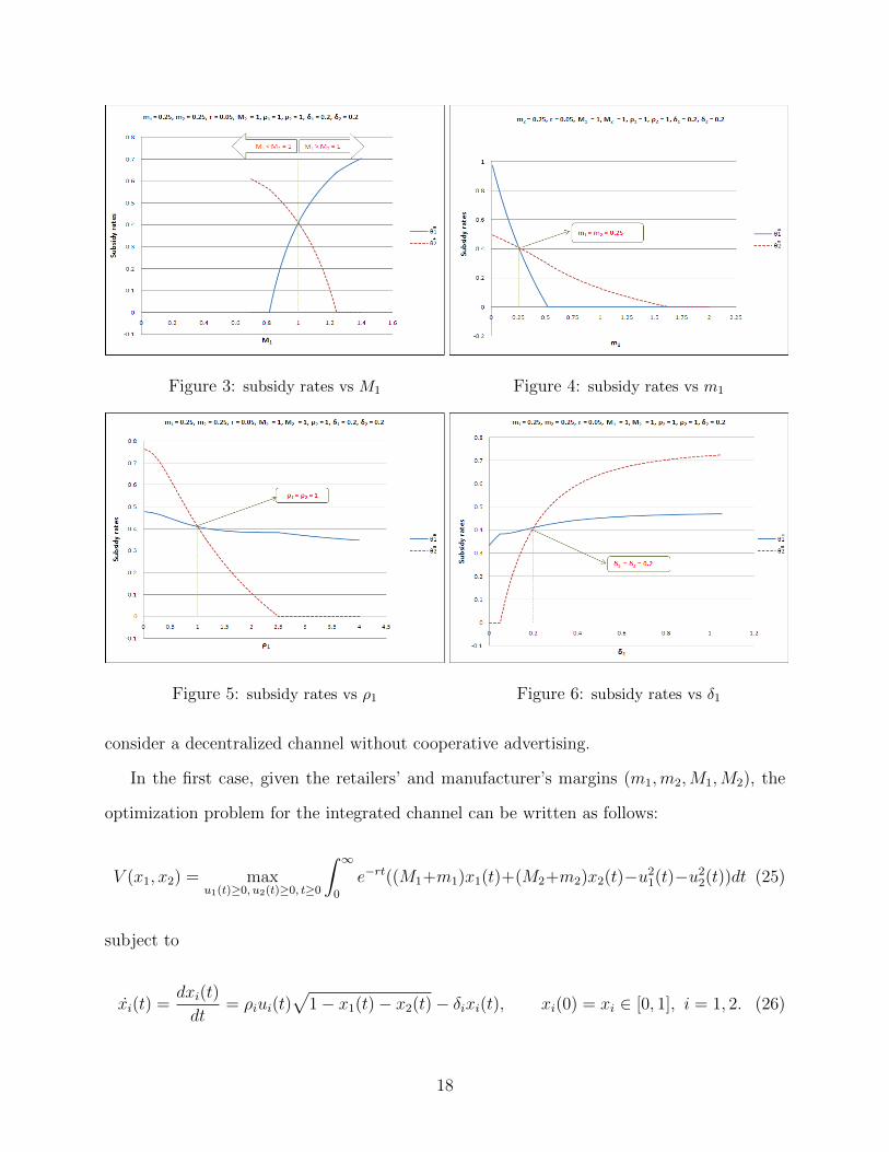
Figure 3: subsidy rates vs M1 Figure 4: subsidy rates vs m1
Figure 5: subsidy rates vs ρ1 Figure 6: subsidy rates vs δ1
consider a decentralized channel without cooperative advertising.
In the first case, given the retailers’ and manufacturer’s margins (m1,m2,M1,M2), the
optimization problem for the integrated channel can be written as follows:
V (x1, x2) = maxu1(t)≥0, u2(t)≥0, t≥0
∫ ∞0
e−rt((M1+m1)x1(t)+(M2+m2)x2(t)−u21(t)−u22(t))dt (25)
subject to
xi(t) =dxi(t)
dt= ρiui(t)
√1− x1(t)− x2(t)− δixi(t), xi(0) = xi ∈ [0, 1], i = 1, 2. (26)
18
The HJB equation for the value function V is
rV (x1, x2) = maxu1≥0,u2≥0
[(M1 +m1)x1 + (M2 +m2)x2 − u21 − u22 + Vx1x1 + Vx2x2], (27)
where x1 and x2 are given by (26). Using (26) in the HJB equation (27) and applying the
first-order conditions for maximization w.r.t. u1 and u2 give the following result.
Proposition 4: For the integrated channel, the optimal feedback advertising policies are
u∗1 =1
2ρ1Vx1
√1− x1 − x2, u∗2 =
1
2ρ2Vx2
√1− x1 − x2, (28)
and the integrated channel’s value function satisfies
4rV (x1, x2) = 4(M1+m1−Vx1δ1)x1+4(M2+m2−Vx2δ2)x2+(1−x1−x2)(V 2x1ρ21+V 2
x2ρ22). (29)
Once again, we conjecture a linear value function of the form V (x1, x2) = αI + βI1x1 + βI2x2,
where αI , βI1 = Vx1 and βI2 = Vx2 are constants, and solve the following system of equations:
4rαI = βI2
1ρ21 + βI
2
2ρ22, (30)
4rβIi = 4(mi +Mi)− 4βIi δi − βI2
i ρ2i − βI
2
3−iρ23−i, i = 1, 2, (31)
The set of equations (30)-(31) is obtained by comparing the coefficients of x1 and x2, and
the constant terms in (29) with βI1(= Vx1), βI2(= Vx2), and αI , respectively.
In the second case, we have a decentralized channel with cooperative advertising, for
which we define the channel value function as V c(x1, x2) = V cm(x1, x2) + V c
r (x1, x2), where
V cm is the manufacturer’s value function (given by (13)) and V c
r is the total value function of
both retailers (obtained by (12) for i = 1, 2.)
In the third case, namely, a decentralized channel with no cooperation, the channel
value function is defined as V n(x1, x2) = V nm(x1, x2) + V n
r (x1, x2), where V nm and V n
r are
19
the manufacturer’s value function and the sum of the two retailers’ value functions in the
non-cooperative setting, respectively. These are computed by simply setting θ∗1 = θ∗2 = 0 in
(15)-(19) and then using (12)-(13).
Before we proceed further, let us observe that the manufacturer is the leader and he
obtains his optimal subsidy rates by maximizing his objective function. Therefore, it should
be obvious that
V cm(x1, x2) ≥ V n
m(x1, x2). (32)
Thus, it remains to study the effect of cooperative advertising on the retailers’ profits and
the total channel profit. First, we examine this in the simple case of symmetric retailers.
We now present the following result.
Proposition 5: In the case of symmetric retailers, the value functions V cr (x1, x2) and
V nr (x1, x2) depend only on the sum (x1 + x2), and can thus be expressed as V c
r (x1 + x2)
and V nr (x1 + x2), with a slight abuse of notation. Furthermore, we have
V cr (x1 + x2) ≥ V n
r (x1 + x2). (33)
The proof of Proposition 5 is provided in Appendix C. It is clear from (32) and (33) that in
the symmetric case, cooperative advertising can partially coordinate the channel, and that
the manufacturer as well as the retailers are better off with cooperative advertising than
without it.
We now return to the general case where explicit analytical relationships between various
value functions are difficult to establish. We, therefore, resort to numerical analysis, and
report our findings based on the results obtained. We compare V, V c, and V n with varying
values of the optimal subsidy rates. Since the value functions depend on the state (x1, x2),
the analysis was carried out for different values of (x1, x2).
We would like to study V, V c, and V n with respect to the changes in the optimal subsidy
rates brought about by changes in the model parameters; for this we consider varying retailer
20
1’s margin. As m1 increases, we know from Fig. 4, that the subsidy rates for both retailers
decrease. As a result, we can compare the various value functions as m1 increases or, roughly
speaking, as subsidy rates decrease. Fig. 7 depicts the values of V, V c, and V n for x1 =
x2 = 0.3. The data range for the calculations shown are the same as those used for the
results shown in Fig. 4. Thus, for any point in Fig. 7, the values of the optimal subsidy
rates are the same as the corresponding values in Fig. 4. Recall that as m1 increases, the
overall cooperation by the manufacturer decreases. It is found that under all instances, V
is greater than V c as well as V n. This is understandable as we expect the channel value
function in the integrated case to be higher than in the decentralized case, with or without
cooperative advertising. In the scenario where both retailers get advertising support, we
find that V c > V n, indicating that the channel attains partial coordination. Moreover, it
is found that the difference V − V c is minimum at the point when both retailers receive
equal positive subsidy rates, and it increases as the difference between the two subsidy rates
increases. These results indicate that the level of coordination achieved is maximum when
both retailers receive equal positive subsidy rates.
An interesting, perhaps even counter-intuitive, observation is that in the case when it
is optimal for the manufacturer to support only one retailer, we find that the overall value
function of the channel in the non-cooperative scenario is slightly higher than in the cooper-
ative case. Thus, from the channel’s perspective, it is better in this case not to support any
retailer than to support only one of the two.
This analysis was carried out for changes in parameters m1, ρ1 and δ1 with the corre-
sponding changes in the optimal subsidy rates as shown in Figs. 4, 5 and 6, respectively, as
well as for different values of (x1, x2). However, we find that the nature of changes in V, V c,
and V n with respect to varying optimal subsidy rates does not change. Fig. 8 shows the
difference in the value functions between the cooperative and non-cooperative settings for
the manufacturer and the two retailers, respectively. As expected, the manufacturer always
benefits from cooperative advertising. One of the retailers, however and surprisingly, do not
21
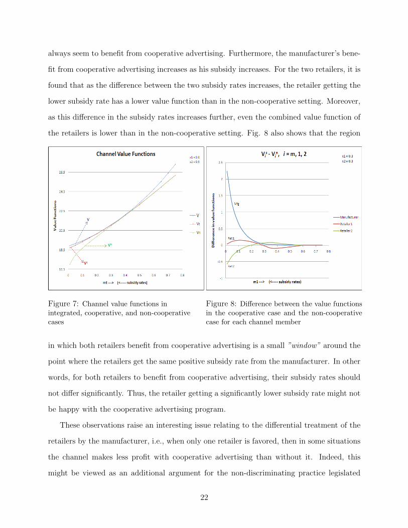
always seem to benefit from cooperative advertising. Furthermore, the manufacturer’s bene-
fit from cooperative advertising increases as his subsidy increases. For the two retailers, it is
found that as the difference between the two subsidy rates increases, the retailer getting the
lower subsidy rate has a lower value function than in the non-cooperative setting. Moreover,
as this difference in the subsidy rates increases further, even the combined value function of
the retailers is lower than in the non-cooperative setting. Fig. 8 also shows that the region
Figure 7: Channel value functions inintegrated, cooperative, and non-cooperativecases
Figure 8: Difference between the value functionsin the cooperative case and the non-cooperativecase for each channel member
in which both retailers benefit from cooperative advertising is a small ”window” around the
point where the retailers get the same positive subsidy rate from the manufacturer. In other
words, for both retailers to benefit from cooperative advertising, their subsidy rates should
not differ significantly. Thus, the retailer getting a significantly lower subsidy rate might not
be happy with the cooperative advertising program.
These observations raise an interesting issue relating to the differential treatment of the
retailers by the manufacturer, i.e., when only one retailer is favored, then in some situations
the channel makes less profit with cooperative advertising than without it. Indeed, this
might be viewed as an additional argument for the non-discriminating practice legislated
22
under such acts as the Robinson-Patman Act of 1936 in the context of price discrimination,
for reasons to enhance competition. In view of these results, we study next the case of
non-discrimination in the context of cooperative advertising.
7 Equal subsidy rate for both retailers
We consider the case when the manufacturer is restricted to offer the same subsidy rate
to both retailers. This case is motivated by possible legal issues that may arise when the
manufacturer discriminates between the two retailers in terms of subsidy rates. Note that
discrimination in terms of price, promotions, discounts, etc. are prohibited by the Robinson-
Patman Act of 1936. Specifically, the Act proscribes discrimination in price between two
or more competing buyers in the sale of commodities of like grade and quality. This and
other anti-discrimination acts, such as the Sherman Antitrust Act of 1890, the Clayton Act
of 1914, and the Celler-Kefauver Act of 1950, prevent discriminatory policies which might
lead to reduced competition and create monopolies in the market.
In our model, different optimal subsidy rates for the two retailers arise from factors such as
the manufacturer’s margins relative to the retailers’ margins, which affect the manufacturer’s
profit. However, if the manufacturer is not allowed to offer different subsidy rates to the re-
tailers, we need to reformulate our problem so that the manufacturer’s optimization problem
has only one subsidy rate decision. In this case, let V RPm (x1, x2), V
RP1 (x1, x2), V
RP2 (x1, x2) and
V RP denote the value functions of the manufacturer, retailer 1, retailer 2, and the total chan-
nel, respectively, with the superscript RP standing for Robinson and Patman. These value
functions solve the control problems defined by (1)-(4) with θ1 = θ2 = θ. Once again, we
expect these value functions to be linear in the market share vector, and express them as in
(12)-(13), except that the coefficients will now be denoted as α, α1, α2, β1, β2, γ1, γ2, B1, and
B2. These coefficients will satisfy the system of equations obtained by setting θ∗1 = θ∗2 = θ∗
23
in (15)-(19). Thus, we have the following equation system: For i = 1, 2,
4rαi = − β2i ρ
2i
(−1 + θ∗)+
2β3−iγiρ23−i
(−1 + θ∗), (34)
4rβi = 4mi − 4βiδi +2β3−iγiρ
23−i
(−1 + θ∗)+
β2i ρ
2i
(−1 + θ∗), (35)
4rγi = −4γiδ3−i +2β3−iγiρ
23−i
(−1 + θ∗)+
β2i ρ
2i
(−1 + θ∗), (36)
rα = − β2i ρ
2i θ∗
4(−1 + θ∗)2+
βiBiρ2i
2(−1 + θ∗)+
β23−iρ
23−iθ
∗
2(−1 + θ∗)2+β3−iB3−iρ
23−i
2(−1 + θ∗), (37)
rBi = Mi − Biδi +β2i ρ
2i θ∗
4(−1 + θ∗)2+
βiBiρ2i
2(−1 + θ∗)+
β23−iρ
23−iθ
∗
4(−1 + θ∗)2+β3−iB3−iρ
23−i
2(−1 + θ∗), (38)
θ∗ = max{ β1(2B1 − β1)ρ21 + β2(2B2 − β2)ρ22β1(2B1 + β1)ρ21 + β2(2B2 + β2)ρ22
, 0}. (39)
The common threshold condition for no cooperation to be optimal is that
P = β1(2B1 − β1)ρ21 + β2(2B2 − β2)ρ22 ≤ 0. (40)
In the case of identical retailers, i.e.,m1 = m2 = m, ρ1 = ρ2 = ρ, and δ1 = δ2 = δ, we
can solve equations (34)-(38) explicitly when θ∗ = 0. The condition for no support by the
manufacturer, with this simplification, reduces to
9(r + δ)2ρ2(M1 +M2)+(2(r + δ)2 −mρ2 −
√4(r + δ)4 + 8m(r + δ)2ρ2 +m2ρ4
)((r + δ)2 +mρ2 +
√4(r + δ)4 + 8m(r + δ)2ρ2 +m2ρ4
)3(r + δ)
≤ 0. (41)
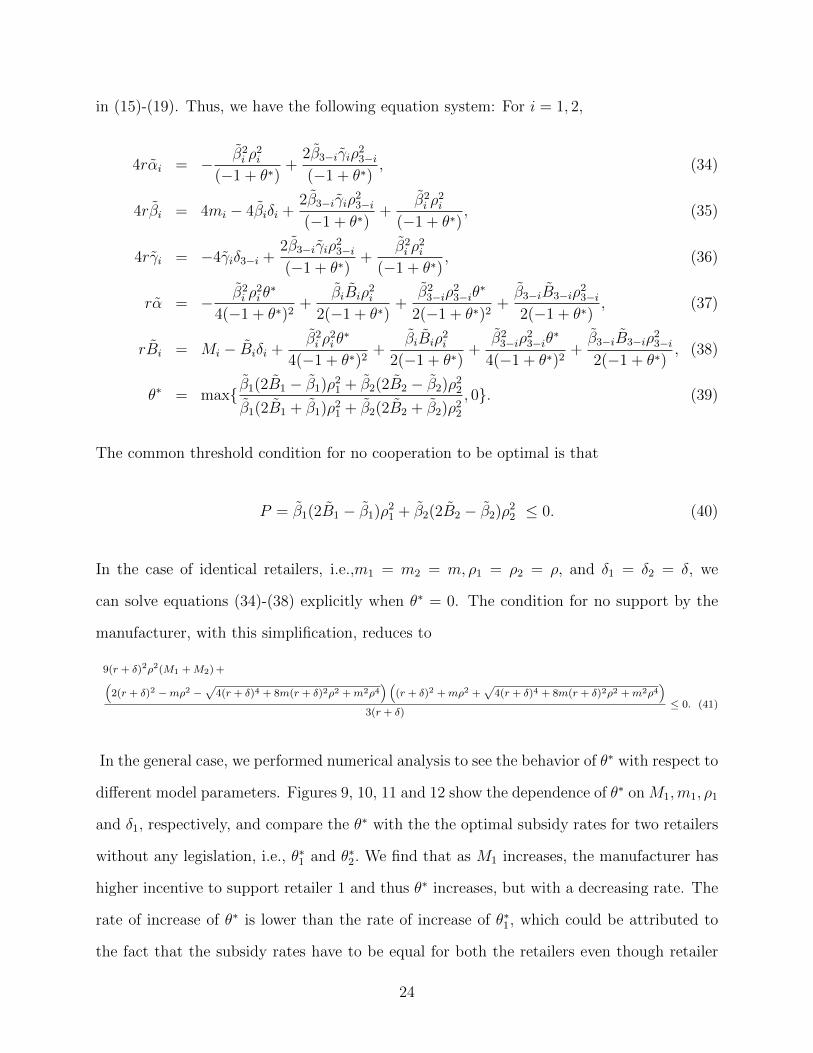
In the general case, we performed numerical analysis to see the behavior of θ∗ with respect to
different model parameters. Figures 9, 10, 11 and 12 show the dependence of θ∗ on M1,m1, ρ1
and δ1, respectively, and compare the θ∗ with the the optimal subsidy rates for two retailers
without any legislation, i.e., θ∗1 and θ∗2. We find that as M1 increases, the manufacturer has
higher incentive to support retailer 1 and thus θ∗ increases, but with a decreasing rate. The
rate of increase of θ∗ is lower than the rate of increase of θ∗1, which could be attributed to
the fact that the subsidy rates have to be equal for both the retailers even though retailer
24
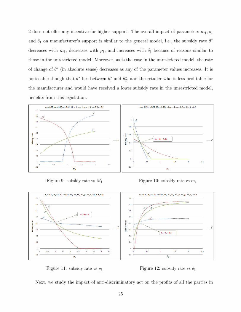
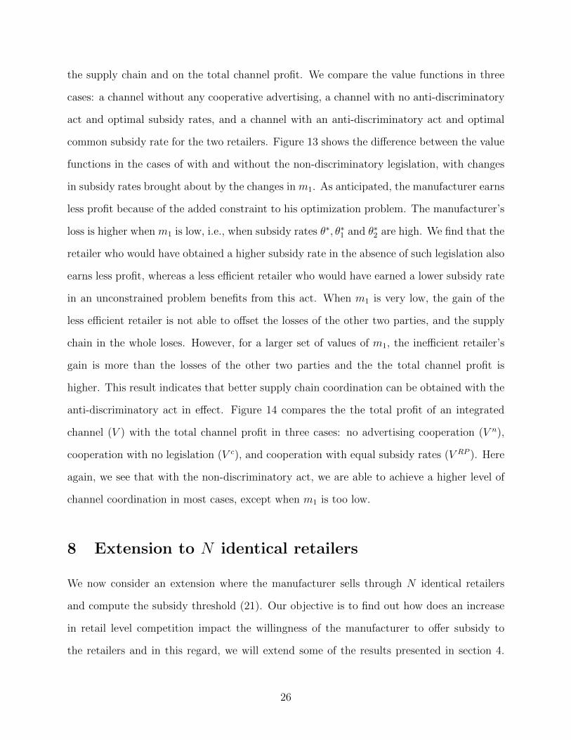
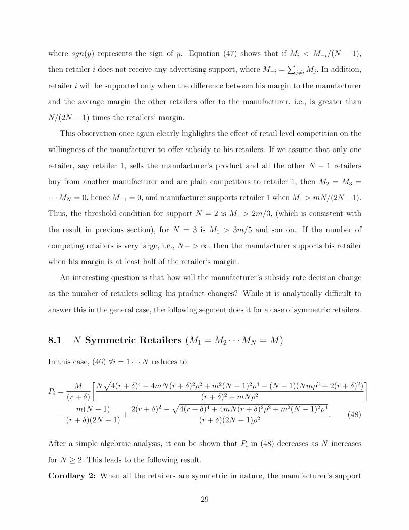
2 does not offer any incentive for higher support. The overall impact of parameters m1, ρ1
and δ1 on manufacturer’s support is similar to the general model, i.e., the subsidy rate θ∗
decreases with m1, decreases with ρ1, and increases with δ1 because of reasons similar to
those in the unrestricted model. Moreover, as is the case in the unrestricted model, the rate
of change of θ∗ (in absolute sense) decreases as any of the parameter values increases. It is
noticeable though that θ∗ lies between θ∗1 and θ∗2, and the retailer who is less profitable for
the manufacturer and would have received a lower subsidy rate in the unrestricted model,
benefits from this legislation.
Figure 9: subsidy rate vs M1 Figure 10: subsidy rate vs m1
Figure 11: subsidy rate vs ρ1 Figure 12: subsidy rate vs δ1
Next, we study the impact of anti-discriminatory act on the profits of all the parties in
25
the supply chain and on the total channel profit. We compare the value functions in three
cases: a channel without any cooperative advertising, a channel with no anti-discriminatory
act and optimal subsidy rates, and a channel with an anti-discriminatory act and optimal
common subsidy rate for the two retailers. Figure 13 shows the difference between the value
functions in the cases of with and without the non-discriminatory legislation, with changes
in subsidy rates brought about by the changes in m1. As anticipated, the manufacturer earns
less profit because of the added constraint to his optimization problem. The manufacturer’s
loss is higher when m1 is low, i.e., when subsidy rates θ∗, θ∗1 and θ∗2 are high. We find that the
retailer who would have obtained a higher subsidy rate in the absence of such legislation also
earns less profit, whereas a less efficient retailer who would have earned a lower subsidy rate
in an unconstrained problem benefits from this act. When m1 is very low, the gain of the
less efficient retailer is not able to offset the losses of the other two parties, and the supply
chain in the whole loses. However, for a larger set of values of m1, the inefficient retailer’s
gain is more than the losses of the other two parties and the the total channel profit is
higher. This result indicates that better supply chain coordination can be obtained with the
anti-discriminatory act in effect. Figure 14 compares the the total profit of an integrated
channel (V ) with the total channel profit in three cases: no advertising cooperation (V n),
cooperation with no legislation (V c), and cooperation with equal subsidy rates (V RP ). Here
again, we see that with the non-discriminatory act, we are able to achieve a higher level of
channel coordination in most cases, except when m1 is too low.
8 Extension to N identical retailers
We now consider an extension where the manufacturer sells through N identical retailers
and compute the subsidy threshold (21). Our objective is to find out how does an increase
in retail level competition impact the willingness of the manufacturer to offer subsidy to
the retailers and in this regard, we will extend some of the results presented in section 4.
26

Figure 13: Value function with anon-discriminatory act minus value functionwithout a non-discriminatory act
Figure 14: Value functions in differentcases divided by integrated channel valuefunction
Following similar notation, we define xi(t) as the market share of retailer i, i = 1, 2 · · ·N, m as
the margin of all the retailers, ρ as the advertising effectiveness coefficient of all the retailers,
δ as the sales decay coefficient of all the retailers, and Mi as the margin of the manufacturer
from retailer i, i = 1 · · ·N. In this case, the state dynamics (1) can be re-written as follows.
For i = 1, 2 · · ·N,
xi(t) = ρiui√
1− x(t)− δixi(t), Xi(0) = xi ∈ [0, 1], (42)
where x(t) =∑N
j=1 xi(t) is the combined market share of the N retailers. Furthermore,
we define the state vector, i.e., the market share vector of N retailers at time t as X(t) =
(x1(t), x2(t) · · · xN(t)), and the subsidy rate vector n feedback form at time t as Θ(X(t)) =
(θ1(X(t)), θ2(X(t)) · · · θN(X(t))), which, for simplicity, will also be be written as X, and
Θ(X), respectively. Now retailer i’s optimization problem (2) can be rewritten as
Vi(X) = maxui(t)≥0, t≥0
∫ ∞0
e−rt(mxi(t)− (1− θi(X))u2i (t))dt, i = 1 · · ·N. (43)
27

The manufacturer anticipates the retailers’ optimal responses and incorporates these into
his optimal control problem, which can now be written as
Vm(X) = max0≤θi(t)≤1,i=1···N, t≥0
∫ ∞0
e−rtN∑j=1
[Mjxj(t)− θi(t) [u1 (X(t) | Θ(t))]2
]dt. (44)
subject to
xi(t) = ρiui(X(t) | Θ(t))√
1− x− δixi(t), xi(0) = xi ∈ [0, 1]. (45)
We solve the HJB equations for the value functions of the retailers and the manufacturer
and by using an approach similar to the one used in analysis for two retailers, we can write
the condition for no advertising support for retailer i. As proved in Appendix B we can we
compute the threshold function Pi for retailer i, i = 1 · · ·N , as
Pi =Mi
(r + δ)
[m(N − 1)ρ2 +
√4(r + δ)4 + 4mN(r + δ)2ρ2 +m2(N − 1)2ρ4
(r + δ)2 +mNρ2
]− M−i
(r + δ)
[2(r + δ)2 +m(N + 1)ρ2 −
√4(r + δ)4 + 4mN(r + δ)2ρ2 +m2(N − 1)2ρ4
(r + δ)2 +mNρ2
]− m(N − 1)
(r + δ)(2N − 1)+
2(r + δ)2 −√
4(r + δ)4 + 4mN(r + δ)2ρ2 +m2(N − 1)2ρ4
(r + δ)(2N − 1)ρ2, (46)
where, M−i =∑
j 6=iMj. We can now conclude the following result
Corollary 1: When Pi ≤ 0, ∀i, i = 1 · · ·N, where Pi, i = 1 · · ·N, is given by (46), it is
optimal for the manufacturer to not support any retailer. Furthermore, if Pk > 0, for some
k ∈ 1 · · ·N and Pj ≤ 0, ∀j, j = 1 · · ·N, j 6= k, then only retailer k is supported and all
others are not. We can also observe that Pi increases with the manufacturer’s margin from
retailers i and decreases as the manufacturer’s margin from any other retailers decreases.
If we assume r ≈ 0 and δ ≈ 0, then the condition of no support for any retailer simplifies.
After taking the appropriate limits, we get
sgn(Pi) = sgn
[Mi −
M−i(N − 1)
− mN
(2N − 1)
], (47)
28
where sgn(y) represents the sign of y. Equation (47) shows that if Mi < M−i/(N − 1),
then retailer i does not receive any advertising support, where M−i =∑
j 6=iMj. In addition,
retailer i will be supported only when the difference between his margin to the manufacturer
and the average margin the other retailers offer to the manufacturer, i.e., is greater than
N/(2N − 1) times the retailers’ margin.
This observation once again clearly highlights the effect of retail level competition on the
willingness of the manufacturer to offer subsidy to his retailers. If we assume that only one
retailer, say retailer 1, sells the manufacturer’s product and all the other N − 1 retailers
buy from another manufacturer and are plain competitors to retailer 1, then M2 = M3 =
· · ·MN = 0, hence M−1 = 0, and manufacturer supports retailer 1 when M1 > mN/(2N−1).
Thus, the threshold condition for support N = 2 is M1 > 2m/3, (which is consistent with
the result in previous section), for N = 3 is M1 > 3m/5 and son on. If the number of
competing retailers is very large, i.e., N− >∞, then the manufacturer supports his retailer
when his margin is at least half of the retailer’s margin.
An interesting question is that how will the manufacturer’s subsidy rate decision change
as the number of retailers selling his product changes? While it is analytically difficult to
answer this in the general case, the following segment does it for a case of symmetric retailers.
8.1 N Symmetric Retailers (M1 = M2 · · ·MN = M)
In this case, (46) ∀i = 1 · · ·N reduces to
Pi =M
(r + δ)
[N√
4(r + δ)4 + 4mN(r + δ)2ρ2 +m2(N − 1)2ρ4 − (N − 1)(Nmρ2 + 2(r + δ)2)
(r + δ)2 +mNρ2
]− m(N − 1)
(r + δ)(2N − 1)+
2(r + δ)2 −√
4(r + δ)4 + 4mN(r + δ)2ρ2 +m2(N − 1)2ρ4
(r + δ)(2N − 1)ρ2. (48)
After a simple algebraic analysis, it can be shown that Pi in (48) decreases as N increases
for N ≥ 2. This leads to the following result.
Corollary 2: When all the retailers are symmetric in nature, the manufacturer’s support
29
will be equal for all the retailers and his tendency to support his retailers decreases as the
number of retailers increases.
A possible explanation of this result is that as N increases, the competition among retailers
for the market share increases and the retailers themselves have an incentive to advertise on
their own accord to increase their respective sales. Then, the manufacturer need not provide
as much advertising support. Furthermore, when (r + δ) ≈ 0, then Pi < 0 ∀i, i = 1 · · ·N ;
and no retailer gets any support, which can also be verified by (47).
9 An Extension: Model with Pricing Decisions
Thus far, we have solved the problem with given margins Mi and mi, i = 1, 2, for the
manufacturer from the two retailers and for the retailers, respectively. We now consider an
extension which includes optimal wholesale and retail price decisions for the manufacturer
and the retailers, respectively. We assume that the manufacturer complies with the legis-
lation forbidding price discrimination and sells to the two retailers at the same wholesale
price. The manufacturer now decides his wholesale price, defined as w(x1, x2), and the sub-
sidy rates θi(x1, x2), i = 1, 2, in feedback form, and the retailers in response choose their
optimal retail prices, denoted as pi(x1, x2) and their advertising efforts ui(x1, x2), i = 1, 2,.
We assume that the manufacturer incurs a per unit constant cost of production, denoted
by c. Furthermore, D(p1, p2) denotes the total demand of the product, and we assume that
∂D(p1,p2)∂pi
< 0, i = 1, 2. The retailer i’s optimization problem is now given by
Vi(x1, x2) = maxpi(t),ui(t)≥0,t≥0
∫ ∞0
e−rt{
(pi(t)− w(x1(t), x2(t)))D(p1, p2)xi(t)
− (1− θi(x1(t), x2(t)))u2i (t)}dt, i = 1, 2, (49)
subject to (1). The manufacturer’s problem is
30
Vm(x1, x2) = max0≤w(t),0≤θi(t)≤1, i=1,2, t≥0
∫ ∞0
e−rt2∑i=1
{(w(t)− c)D(p1, p2)xi(t)
− θi(t) [ui (x1(t), x2(t) | w(t), θ1(t), θ2(t))]2
}dt i = 1, 2, (50)
subject to
xi(t) = ρiui(x1(t), x2(t) | w(t), θ1(t), θ2(t))√
1− x1(t)− x2(t)− δixi(t),
xi(0) = xi ∈ [0, 1], i = 1, 2. (51)
We can see that in the problems defined by (1), (49)-(51), the wholesale and the retail prices
appear only in the profit functions and not in the state equations. Thus, we can compute the
optimal retail and wholesale prices by maximizing the retailers’ and the manufacturer’s profit
functions, respectively. Here again, we first compute the optimal retail price and incorporate
the retailers’ response to solve for the wholesale price. By writing the first-order conditions
w.r.t. pi, i = 1, 2, and w we get the following result.
Proposition 6: For a given wholesale price w(x1, x2), the equilibrium retail prices p∗i =
p∗i (x1, x2 | w, θ1, θ2), i = 1, 2, are given as the solution of the equations
D(p∗1, p∗2) + (p∗i − w)
∂D(p1, p2)
∂pi
∣∣∣∣p1=p∗1,p2=p
∗2
= 0, i = 1, 2. (52)
Furthermore, equilibrium wholesale price w∗ = w∗(x1, x2) solves
(w∗ − c) ∂D(p∗1, p∗2)
∂w
∣∣∣∣w=w∗
+D(p∗1, p∗2) = 0. (53)
The optimal margins for the retailers and the manufacturer can be written as m∗i = (p∗i −
w∗)D(p∗1, p∗2), i = 1, 2, and M∗ = (w∗ − c)D(p∗1, p
∗2). Using these margins the optimization
problems for the retailers and the manufacturer reduces to (2) and (3), respectively, by
31
simply using mi = m∗i ,M1 = M2 = M∗.
Remark: With wholesale price as a decision of the manufacturer the application of the
price non-discrimination legislation yields M1 = M2 whereas we have permitted M1 6= M2
in our original formulation in Section 2 where these margins are given. This is because the
additional generality does not present any difficulty in the analysis of the model when the
margins are not decision variables and the possibility that these margins result of not only
just the wholesale prices, but also some other considerations allowed in the law. However, if
we were to allow different wholesale prices for the retailers, then the optimal wholesale prices
and consequently the margins become functions of the state, and the problem becomes far
too complex to permit a solution in explicit form, as achieved in the preceding sections for
our original model with given margins.
10 Concluding Remarks
We consider a cooperative advertising model with a manufacturer supplying to one or both of
two retailers, and formulate it as a Stackelberg differential game. We obtain the Stackelberg
feedback equilibrium and derive the conditions under which there will or will not be any
cooperative advertising. We also provide the sensitiveness of the optimal subsidy rates with
respect to the various problem parameters. We examine the issue of channel coordination
with cooperative advertising and find that partial coordination can be achieved when both
retailers are supported. When only one of the retailers is supported, there are cases when
the manufacturer’s gain from cooperative advertising does not offset the loss incurred by
the retailers. This leads us also to examine the model when the manufacturer is required to
offer the same subsidy rates to both retailers, in the spirit of non-discriminating legislations
such as the Robinson-Patman Act of 1936. We find that the optimal common subsidy rate
lies between the two optimal subsidy rates that would prevail in the absence of any such
legislation. We find that the legislation benefits the less efficient retailer, and takes away
32

some profits from the manufacturer and the other retailer. We also see evidence of a higher
channel profit and better supply chain coordination with the legislation. Furthermore, the
presence of a second retailer allows us to study the effect of the retail level competition absent
in He et al. (2009). In the case when the second retailer does not sell the manufacturer’s
product but competes with the retailer selling the manufacturer’s product, we find that the
manufacturer supports his retailer under a larger set of conditions than those in He et al.
(2009).
We also study an extension with any number of retailers and an extension in which
wholesale prices and retail prices are also decision variables for the manufacturer and re-
tailers, respectively. In the extension with N identical retailers when only one retailer sells
the manufacturer’s product and the remaining retailers are competitors, we show that the
manufacturer’s threshold to start supporting his retailers eases as the number of competing
retailers increases. Furthermore, when all of the retailers sell the manufacturer’s product,
we show that the manufacturer’s tendency to provide support to each retailer decreases as
the number of retailers increases.
Appendices
A Derivation of Pi, i = 1, 2, for two identical retailers
For two identical retailers, the system (15)-(20) can be reduced to the following equations in
four coefficients βi, Bi, i = 1, 2, only:
βi =−(r + δ)(r + δ + β3−iρ
2) +√
(r + δ)(r + δ + β3−iρ2)((r + δ)2 + (2m+ β3−i(r + δ))ρ2)
(r + δ)ρ2,
Bi =Mi −Biδ − (βiBi + β3−iB3−i)ρ
2
r, i = 1, 2.
These equations can be solved explicitly to get βi and Bi for i = 1, 2, as follows:
33
β1 = β2 =−2(r + δ)2 +mρ2 +
√4(r + δ)4 + 8m(r + δ)2ρ2 +m2ρ4
3(r + δ)ρ2, (A.1)
Bi =2(2Mi +M3−i)(r + δ)2 + (Mi −M3−i)(mρ
2 +√
4(r + δ)4 + 8m(r + δ)2ρ2 +m2ρ4)
2(r + δ)((r + δ)2 +mρ2 +√
4(r + δ)4 + 8m(r + δ)2ρ2 +m2ρ4).
(A.2)
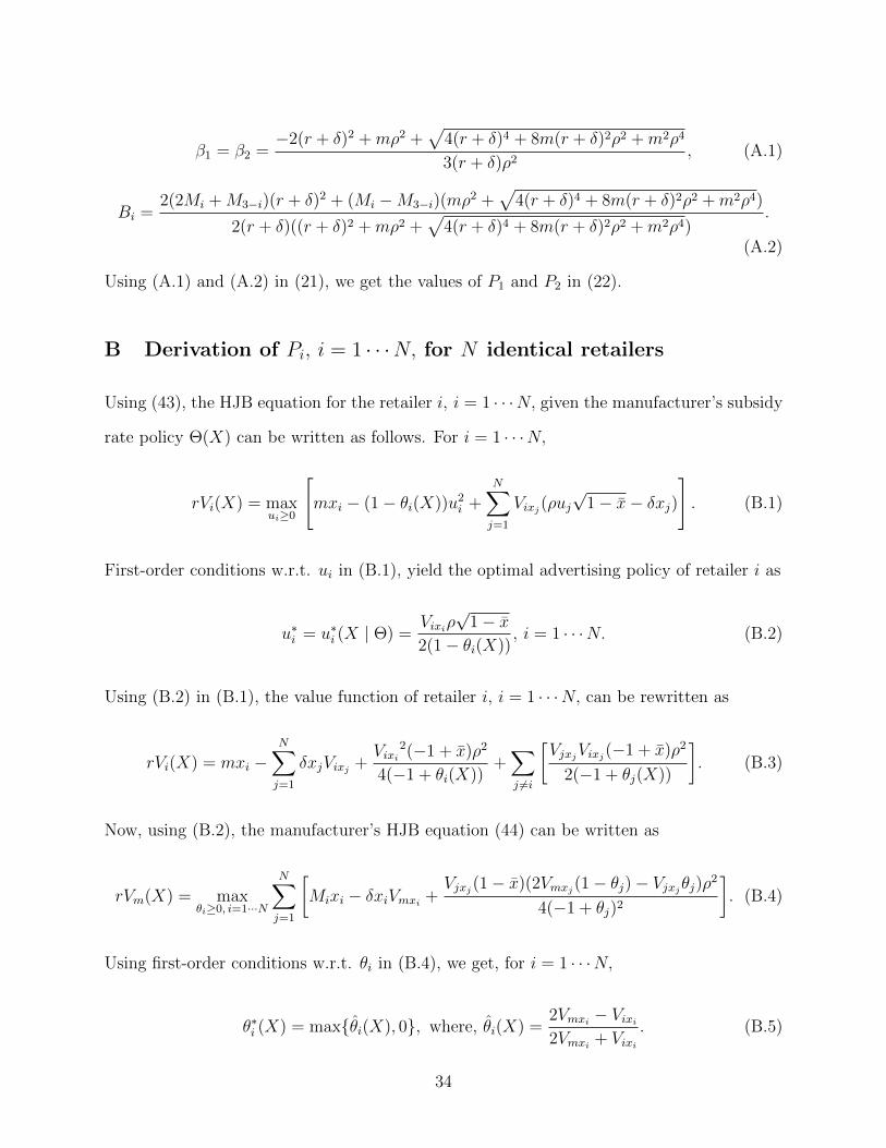
Using (A.1) and (A.2) in (21), we get the values of P1 and P2 in (22).
B Derivation of Pi, i = 1 · · ·N, for N identical retailers
Using (43), the HJB equation for the retailer i, i = 1 · · ·N, given the manufacturer’s subsidy
rate policy Θ(X) can be written as follows. For i = 1 · · ·N,
rVi(X) = maxui≥0
[mxi − (1− θi(X))u2i +
N∑j=1
Vixj(ρuj√
1− x− δxj)
]. (B.1)
First-order conditions w.r.t. ui in (B.1), yield the optimal advertising policy of retailer i as
u∗i = u∗i (X | Θ) =Vixiρ
√1− x
2(1− θi(X)), i = 1 · · ·N. (B.2)
Using (B.2) in (B.1), the value function of retailer i, i = 1 · · ·N, can be rewritten as
rVi(X) = mxi −N∑j=1
δxjVixj +Vixi
2(−1 + x)ρ2
4(−1 + θi(X))+∑j 6=i
[VjxjVixj(−1 + x)ρ2
2(−1 + θj(X))
]. (B.3)
Now, using (B.2), the manufacturer’s HJB equation (44) can be written as
rVm(X) = maxθi≥0, i=1···N
N∑j=1
[Mixi − δxiVmxi +
Vjxj(1− x)(2Vmxj(1− θj)− Vjxjθj)ρ2
4(−1 + θj)2
]. (B.4)
Using first-order conditions w.r.t. θi in (B.4), we get, for i = 1 · · ·N,
θ∗i (X) = max{θi(X), 0}, where, θi(X) =2Vmxi − Vixi2Vmxi + Vixi
. (B.5)
34
We now use the optimal subsidy rate policy of the manufacturer given by (B.5) in the HJB
equation (B.4) to rewrite the manufacturer’s value function as
rVm(X) =N∑j=1
[Mjxj − δxjVmxj +
Vjxj(1− x)(2Vmxj(1− θ∗j (X))− Vjxjθ∗j (X))ρ2
4(−1 + θ∗j (X))2
](B.6)
Once again, we conjecture linear value functions of the following form,
Vi(X) = αi + βixi +∑j 6=i
γijxj, i = 1 · · ·N, j = 1 · · ·N, j 6= i (B.7)
Vm(X) = α +N∑j=1
Bjxj, (B.8)
and try to solve for the coefficients αi, βi, γij, α and Bi, i = 1 · · ·N, j = 1 · · ·N, j 6= i. We
can see that βi = Vixi , γij = Vixj , Bi = Vmxi , i = 1 · · ·N, j = 1 · · ·N, j 6= i. We compare the
terms of xi, i = 1 · · ·N, and the constant terms of the value functions in the equations (B.3)
and (B.6) with the corresponding terms in (B.7)-(B.8) and we get the following system of
equations to be solved in the coefficients βi, γij, Bi, i = 1 · · ·N, i = 1 · · ·N, j 6= i.
4rαi = − β2i ρ
2
(−1 + θ∗i )+∑j 6=i
2βjγijρ2
(−1 + θ∗j ), (B.9)
4rβi = 4m− 4βiδ +∑j 6=i
2βjγijρ2
(−1 + θ∗j )+
β2i ρ
2
(−1 + θ∗i ), (B.10)
4rγij = −4γijδ +∑j 6=i
2βjγijρ2
(−1 + θ∗j )+
β2i ρ
2
(−1 + θ∗i ), (B.11)
rα = −N∑j=1
βj(2Bj(−1 + θ∗j (X)) + βjθ∗j(X))ρ2
4(−1 + θ∗j )2
, (B.12)
rBi = Mi −Biδ +N∑j=1
βj(2Bj(−1 + θ∗j (X)) + βjθ∗j(X))ρ2
4(−1 + θ∗j )2
, (B.13)
θ∗i = max{2Bi − βi2Bi + βi
, 0}. (B.14)
To compute the condition under which the manufacturer will support a retailer, we let
35
Pi = 2Vmxi − Vixi = Bi − βi, i = 1, 2, · · ·N. (B.15)
Thus, when Pi > 0, the manufacturer supports retailers i, otherwise he does not. When
Pi < 0, ∀i, i = 1, 2, · · ·n, θ∗i = 0, ∀i, i = 1, 2, · · ·n, and equations (B.9)-(B.11) can be solved
independently of (B.12)-(B.13). Using θ∗i = 0, ∀i = 1, 2, · · ·n, in (B.9)-(B.13) we can solve
for the coefficients βi, αi, γij, α, and Bi, ∀i = 1, 2, · · ·n, and using these values in (B.15), we
can get the values of Pi, ∀i = 1, 2, · · ·n, as shown in (46).
C Proof of Proposition 5
As defined in section 7, V cr is the combined value function of the two retailers in the cooper-
ative scenario and V nr is the same in the non-cooperative scenario. We can write γi and αi in
terms of βi from (D.1) and (D.3), respectively. Recall that in the case of symmetric retailers,
α1 = α2 = α, β1 = β2 = β, and γ1 = γ2 = γ. Furthermore, when there is no cooperation,
β = η, and its value is given by (A.1). Using β = η, (D.1), and (D.3), we can find V nr by
adding computing (12) for i = 1, 2, and adding the two. After a few steps of algebra, we get
V nr =
2(x1 + x2)(m(r + 2δ)− 2δ(r + δ)η1) + (−1 + x1 + x2)η1(2m− 3(r + δ)η1)ρ2
2r(r + δ). (C.1)
In the case of symmetric retailers with cooperation, using (D.1) and (D.3) from Appendix
D, and using the fact that α1 = α2 = α, β1 = β2 = β and γ1 = γ2 = γ, we get
V cr =
4(x1 + x2)(m(r + 2δ)− 2βδ(r + δ))− (β + 2B)(1− x1 − x2)(2m− 3β(r + δ))ρ2
4r(r + δ).
(C.2)
Clearly, V nr and V c
r depend only on the sum (x1 +x2), and this proves the first statement
of Proposition 5. Next, we define ∆Vr = V cr − V n
r , which can be computed as follows
∆Vr =−8xδ(r + δ)(β − η1) + (−1 + x)(2m(β + 2B − 2η1)− 3(r + δ)(β2 + 2Bβ − 2η21))ρ2
4r(r + δ),
36
where x = x1 + x2. ∆Vr is linear in x, and we will write it as ∆Vr(x). We can see that
∆Vr(1) = 2δ(η1−β)/r > 0. This is because we know from (B.14) that to sustain a cooperative
equilibrium, the parameters (m,M, r, δ, ρ) should be such that β < η1.
Now consider
∆Vr(0) =(−2m(β + 2B − 2η1) + 3(r + δ)(β2 + 2Bβ2 − 2η21))ρ2
4r(r + δ).
Substituting the value of B in terms of β (from (D.10)) in the above expression, we can write
∆Vr(0) =4(r + δ)(m− β(r + δ)) + η(2m− 3(r + δ)η)
2r(r + δ). (C.3)
It is clear by (C.3) that a decrease in the value of β (caused by changes in parameters) also
decreases the value of ∆Vr(0). We know that for a cooperative equilibrium, β < η1, and so
a lower bound for ∆Vr(0) can be obtained by using β = η1 in (C.3). This lower bound is
4m(r + δ) + 2mηρ2 − (r + δ)η(4(r + δ) + 3ηρ2)
2r(r + δ).
By using the value of η1 from Appendix D, and after a few steps of algebra, we can see that
the above expression reduces to zero. Therefore, ∆Vr(0) > 0.
Because ∆Vr(x) is linear in x, ∆Vr(0) > 0, and ∆Vr(1) > 0, we can say that ∆Vr(x) >
0,∀x ∈ [0, 1]. Thus, V cr (x) > V n
r (x),∀x ∈ [0, 1]. The equality holds when β = η1, i.e., when
non-cooperation is optimal for the manufacturer.
D Uniqueness of optimal solution in the case of two symmetric
retailers
The uniqueness of an optimal solution to the problem defined by (6), (7), (9), (10), and
(11) is guaranteed by a unique solution of the system of equations (15)-(20). It appears
37

to be difficult to prove the uniqueness in the general case. However, in the special case
of symmetric retailers (M1 = M2 = M,m1 = m2 = m, δ1 = δ2 = δ and ρ1 = ρ2), we can
establish the result as follows.
We first look at the signs of αi, βi and γi, i = 1, 2. It is expected that βi > 0. Now
consider γi, which can be expressed in terms of β1 and β2 by using equation (17):
γi =β2i (−1 + θ∗3−i)ρ
2i
2(−1 + θ∗i )((r + δ3−i)(−1 + θ∗3−i)− β3−iρ23−i), i = 1, 2.
Since βi > 0 and θ∗i < 1, i = 1, 2, we have γi = Vix3−i < 0, as intuition would suggest on
account of the competition between the retailers. We can also use (16) and (17) to write
γi =−mi + βi(r + δi)
(r + δ3−i). (D.1)
Since γi < 0, we must have
βi <mi
(r + δi). (D.2)
Now consider αi, which is retailer i ’s value function when the initial market is zero for
both retailers. We now show that this value is positive. By adding (15) and (17), we can
conclude that αi = −γi(r + δ3−i)/r, which is positive since γi < 0. Thus,
αi =mi − βi(r + δi)
r> 0. (D.3)
Moreover, using (D.1) in equation (15), we can write αi in terms of β1 and β2, and then
rewrite (D.3) as
αi =1
4r
[2β3−i(mi − βi(r + δi))ρ
23−i
(r + δ3−i)(−1 + θ3−i)− β2
i ρ2i
(−1 + θi)
]> 0, i = 1, 2. (D.4)
Clearly, in the symmetric case, we will have α1 = α2 = α, β1 = β2 = β, γ1 = γ2 =
38
γ, B1 = B2 = B, and hence θ∗1 = θ∗2 = θ∗. We can thus rewrite (D.4) as
β(2m− 3β(r + δ))ρ2
2r(r + δ)(−1 + θ)> 0.
This, along with β > 0 and θ < 1, gives us
β >2m
3(r + δ). (D.5)
From (D.2) and (D.5), we have
2m
3(r + δ)< β <
m
(r + δ). (D.6)
To prove a unique solution to equations (15)-(20), we reduce them into one equation of a
single variable β, and then aim for the unique solution of β. We will separately consider the
cases of a cooperative equilibrium where θ∗ > 0 and a non-cooperative equilibrium where
θ∗ = 0.
Case I: Cooperative equilibrium (θ∗ > 0.)
Since β1 = β2 = β and B1 = B2 = B in the symmetric case, (20) reduces to θ∗ = (2B −
β)/(2B+β). Using this, (D.1), and (D.3), we can reduce equations (15)-(20) to two equations
in variables β and B, i.e.,
4r(r + δ)β = 4(r + δ)(m− βδ) + (β + 2B)(2m− 3β(r + δ))ρ2 (D.7)
4rB = 4M − 4Bδ − (β + 2B)2ρ2. (D.8)
Using (D.7), (D.8) and (14) in (21) and setting P1 = P2 = P on account of the case being
39
symmetric, we obtain the participation threshold function
P = 2B − β =8(r + δ)(−m+ 2M + (β − 2B)δ)− (β + 2B)(2m− (β − 4B)(r + δ))ρ2
8r(r + δ).
(D.9)
Using (D.7), we can write B in terms of β as follows:
B =−2m(4(r + δ) + βρ2) + β(r + δ)(8(r + δ) + 3βρ2)
2(2m− 3β(r + δ))ρ2. (D.10)
Now using (D.9) and (D.10), we can rewrite P in terms of β only, and then write the condition
of the cooperative equilibrium as
P =−4m((r + δ)2 + βρ2) + 2β(r + δ)(4(r + δ) + 3βρ2)
(2m− 3β(r + δ))ρ2> 0. (D.11)
Next, we find the values of β for which the inequality in (D.11) holds. In order to see how
P varies with β, we first find the roots of the equation P = 0. The numerator is quadratic
in β with the roots denoted as η1 and η2:
η1 =−2(r + δ)2 +mρ2 +
√4(r + δ)4 + 8m(r + δ)2ρ2 +m2ρ4
3(r + δ)ρ2
η2 =−2(r + δ)2 +mρ2 −
√4(r + δ)4 + 8m(r + δ)2ρ2 +m2ρ4
3(r + δ)ρ2.
Clearly, η1 > 0 and η2 < 0. Also, the denominator (2m−3β(r+ δ))ρ2 of (D.11) changes sign
at β = 2m/3(r + δ); the denominator is strictly positive when β < 2m/3(r + δ) and strictly
negative when β > 2m/3(r + δ).
We will now compare the value of η1 with m/(r + δ) and 2m/3(r + δ). We can see that
the difference
η1 −2m
3(r + δ)=−2(r + δ)2 −mρ2 +
√4(r + δ)4 + 8m(r + δ)2ρ2 +m2ρ4
3(r + δ)ρ2> 0,
40
and thus η1 > 2m/3(r + δ). Furthermore,
η1 −m
(r + δ)=−2(r + δ)2 − 2mρ2 +
√4(r + δ)4 + 8m(r + δ)2ρ2 +m2ρ4
3(r + δ)ρ2< 0,
and thus we have
2m
3(r + δ)< η1 <
m
(r + δ). (D.12)
We can then conclude from (D.11) that P > 0 is satisfied when
β ∈ (−∞,−η2) or β ∈ (2m
3(r + δ), η1). (D.13)
Therefore, the conditions (D.6), (D.12) and (D.13) along with the fact that β > 0 give us
the desirable range of the solution for β, i.e.,
β ∈ (2m
3(r + δ), η1). (D.14)
Now using (D.10) in (D.8), we can write a single equation in β. After some steps of algebra,
for the symmetric retailer case with positive cooperation, this single equation for β can be
written as
F (β) =8β(r + δ)3(m− β(r + δ))− (2m− 3β(r + δ))2(2M + β(r + δ))ρ2
(2m− 3β(r + δ))2ρ2= 0.
Thus, a unique cooperative solution in the symmetric retailer case is guaranteed when exactly
one root of the equation F (β) = 0 lies in the range given by (D.14). The numerator of the
above expression, denoted as N(β), is cubic in β. Thus, we can rewrite the equation for β
as
N(β) = aβ3 + bβ2 + cβ + d = 0, (D.15)
41
where
a = −9(r + δ)3ρ2, b = −8(r + δ)4 + 6(2m− 3M)(r + δ)2ρ2,
c = 4m(r + δ)(2(r + δ)2 − (m− 6M)ρ2) and d = −8m2Mρ2.
Since the denominator of F (β) is positive for all values of β except 2m/3(r + δ), the sign
of F (β) is the same as that of N(β). In what follows, we perform a simple sign analysis of
N(β) to draw inference about the roots of (D.15). After a few steps of algebra with the help
of Mathematica, the following observations can be made
N(β)→∞ as β → −∞;
N(β) = −8m2Mρ2 < 0 when β = 0;
N(β) =16
9m2(r + δ)2 > 0 when β =
2m
3(r + δ);
N(β) = −m2(m+ 2M)ρ2 < 0 when β =m
(r + δ);
N(β)→ −∞ as β →∞.
These observations make it clear that the equation N(β) = 0 has three real roots in the
following intervals:
(−∞, 0), (0,2m
3(r + δ)) and (
2m
3(r + δ),
m
(r + δ)).
Moreover, from (D.12) and (D.14), we see that there should be exactly one root in the
desired interval ( 2m3(r+δ)
, η1) for there to be cooperation in the equilibrium solution. In fact,
the location of the third root in the interval ( 2m3(r+δ)
, m(r+δ)
) w.r.t η1 determines whether we
will have a cooperative or non-cooperative equilibrium. Figure 15 shows the curve N(β)
when β > 0. This curve gives us an idea of when exactly one of the two positive roots of the
equation N(β) = 0 would be in the interval ( 2m3(r+δ)
, η1). Note that one root of this equation
42
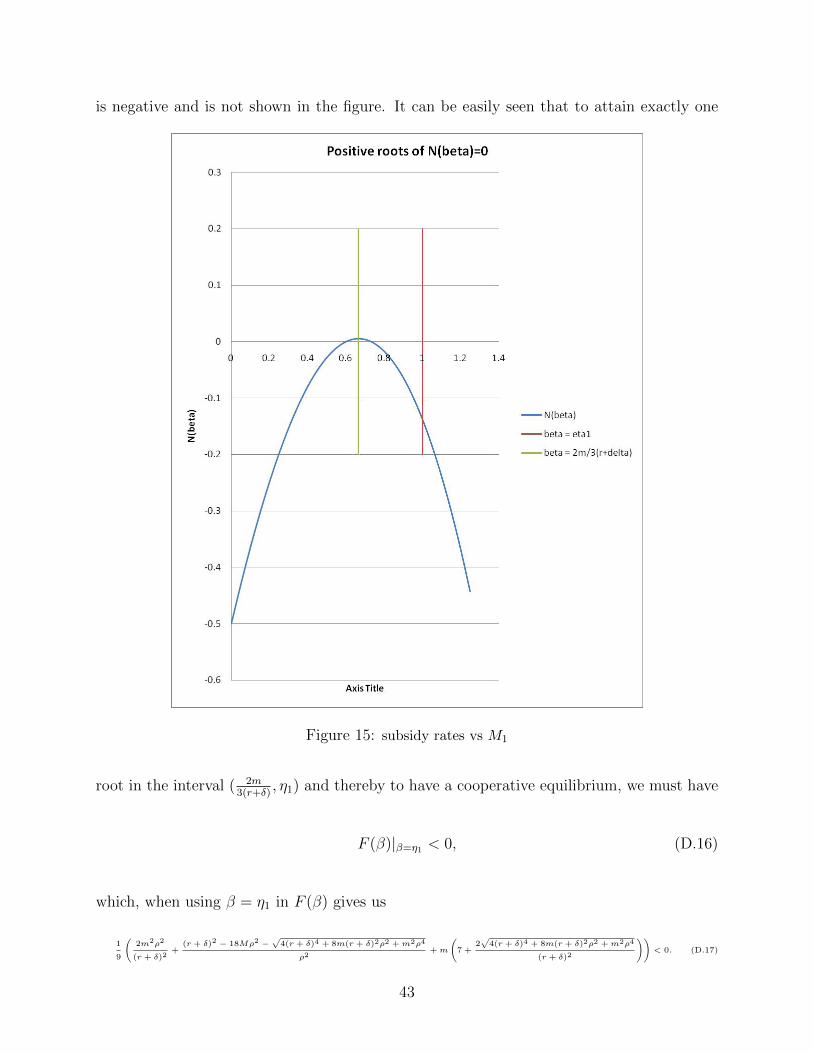
is negative and is not shown in the figure. It can be easily seen that to attain exactly one
Figure 15: subsidy rates vs M1
root in the interval ( 2m3(r+δ)
, η1) and thereby to have a cooperative equilibrium, we must have
F (β)|β=η1 < 0, (D.16)
which, when using β = η1 in F (β) gives us
1
9
(2m2ρ2
(r + δ)2+
(r + δ)2 − 18Mρ2 −√
4(r + δ)4 + 8m(r + δ)2ρ2 +m2ρ4
ρ2+m
(7 +
2√
4(r + δ)4 + 8m(r + δ)2ρ2 +m2ρ4
(r + δ)2
))< 0. (D.17)
43
After a few steps of algebra, one can see that the condition (D.17) has just the opposite
sign to the one that ensures a non-cooperative solution in the case of symmetric retailers,
which can be obtained by simply using M1 = M2 = M in Proposition 3. In other words,
when the parameters m,M, r, δ, and ρ are such that the inequality (D.17) is not satisfied,
then the third root of the equation N(β) = 0 will be greater than or equal to η1, and the
optimal solution will be a non-cooperative one. Thus, a unique cooperative equilibrium is
guaranteed when (D.17) is satisfied.
Case II: Non-Cooperative equilibrium
We now consider the non cooperative equilibrium (θ∗ = 0) in the symmetric retailer case.
As illustrated in Appendix A, the system of equations (15)-(20) can be solved explicitly in
the non-cooperative case to get a unique positive solution of β1 and β2, given by (A.1). Since
the symmetric retailer case is a further simplification of the case of identical retailers, i.e.,
with M1 = M2 = M, the solution of β is unique and is given by (A.1). Note that this value
of β equals η1.
References
1. Berger PD (1972) Vertical cooperative advertising ventures. J. Market. Res. 9(3): 309-
312.
2. Chintagunta PK, Jain DC (1992) A dynamic model of channel member strategies for
marketing expenditures. Market. Sci. 11(2): 168-188.
3. Chintagunta PK, Jain DC (1995) Empirical analysis of a dynamic duopoly model of
competition. J. Econ. Manage. Strat. 4(1): 109-131.
4. Dant RP, Berger PD (1996) Modeling cooperative advertising decisions in franchising.
J. Operat. Res. Soc. 47(9): 1120-1136.
44
5. Deal KR (1979) Optimizing advertising expenditures in a dynamic duopoly. Oper. Res.
27: 682-692.
6. Dutta S, Bergen M, John G, Rao A (1995) Variations in the Contractual Terms of
Cooperative Advertising Contracts: An Empirical Investigation. Market. Lett. 6(1):
15-22.
7. Erickson GM (2009) An oligopoly model of advertising competition. Eur. J. Operat.
Res. 197(1): 374-388.
8. Erickson GM (2009) Advertising competition in a dynamic oligopoly with multiple
brands. Oper. Res. 57(5): 1106-1113.
9. He X, Prasad A, Sethi SP (2009) Cooperative advertising and pricing in a dynamic
stochastic supply chain: feedback Stackelberg strategies. Prod. and. Oper. Mgmt. 18(1):
78-94.
10. He X, Krishnamoorthy A, Prasad A, Sethi SP (2011) Retail competition and cooperative
advertising. Oper. Res. Lett. 39(1): 11-16.
11. Huang Z, Li SX, Mahajan V (2002) An analysis of manufacturer-retailer supply chain
coordination in cooperative advertising. Dec. Sci. 33(3): 469-494.
12. Jørgensen S, Sigue SP, Zaccour G (2000) Dynamic cooperative advertising in a channel.
J. retail. 76(1): 71-92.
13. Jørgensen S, Taboubi S, Zaccour G (2001) Cooperative advertising in a marketing chan-
nel. J. Optim. Theory. Appl. 110(1): 145-158.
14. Jørgensen S, Taboubi S, Zaccour G (2003) Retail promotions with negative brand image
effects: Is cooperation possible? Eur. J. Operat. Res. 150(2): 395-405.
15. Kali R (1998) Minimum advertised price. J. Econ. Manag. strategy 7(4): 647-668.
45
16. Karray S, Zaccour G (2005) A differential game of advertising for national brand and
store brands. A. Haurie, G. Zaccour eds. Dynamic Games: Theory and Applications.
Springer, Berlin, pp 213-229.
17. Little JDC (1979) Aggregate advertising models: The state of the art. Oper. Res. 27:
629-667.
18. Nagler MG (2006) An exploratory analysis of the determinants of cooperative advertis-
ing participation rates. Market. Lett. 17(2): 91-102.
19. Naik PA, Prasad A, Sethi SP (2008) Building brand awareness in dynamic oligopoly
markets. Manag. Sci. 54(1): 129-138.
20. Nerlove M, Arrow KJ (1962) Optimal advertising policy under dynamic conditions.
Economica. 29: 129-142.
21. Prasad A, Sethi SP (2004) Competitive advertising under uncertainty: A stochastic
differential game approach. J. Optim. Theory Appl. 123(1): 163-185.
22. Prasad A, Sethi SP (2009) Integrated marketing communications in markets with un-
certainty and competition. Automatica 45(3): 601-610.
23. Sethi SP (1983) Deterministic and stochastic optimization of a dynamic advertising
model. Optim. Control Appl. Meth. 4(2): 179-184.
24. Sorger G (1989) Competitive dynamic advertising, a modification of the case game. J.
of Econ. Dynam. and Control 13: 55-80.
25. Vidale ML, Wolfe HB (1957) An Operations Research study of sales response to adver-
tising. Operat. Res. 5(3): 370-381.
46