controlling buoyancy-driven profiling floats for applications in ocean observation

This article has been accepted for inclusion in a future issue of this journal. Content is final as presented, with the exception of pagination.

IEEE JOURNAL OF OCEANIC ENGINEERING 1

Controlling Buoyancy-Driven Profiling Floats forApplications in Ocean ObservationRyan N. Smith, Member, IEEE, and Van T. Huynh, Student Member, IEEE

Abstract—Establishing a persistent presence in the ocean withan autonomous underwater vehicle (AUV) capable of observingtemporal variability of large-scale ocean processes requires aunique sensor platform. In this paper, we examine the utility ofvehicles that can only control their depth in the water column forsuch extended deployments. We present a strategy that utilizesocean model predictions to facilitate a basic level of autonomy andenables general control for these profiling floats. The proposedmethod is based on experimentally validated techniques for uti-lizing ocean current models to control autonomous gliders. Withthe appropriate vertical actuation, and utilizing spatio–temporalvariations in water speed and direction, we show that generalcontrollability results can be met. First, we apply an A* plannerto a local controllability map generated from predictions of oceancurrents. This computes a path between start and goal waypointsthat has the highest likelihood of successful execution. A computeddepth plan is generated with a model-predictive controller (MPC),and selects the depths for the vehicle so that ambient currentsguide it toward the goal. Mission constraints are included to sim-ulate and motivate a practical data collection mission. Results arepresented in simulation for a mission off the coast of Los Angeles,CA, USA, that show encouraging results in the ability of a driftingvehicle to reach a desired location.

Index Terms—Autonomous underwater vehicle (AUV), model-predictive control (MPC), ocean model, path planning, profilingfloat.

I. INTRODUCTION

A profiling float is an underwater vehicle that is actuatedonly in the vertical (heave) direction, with the horizontal

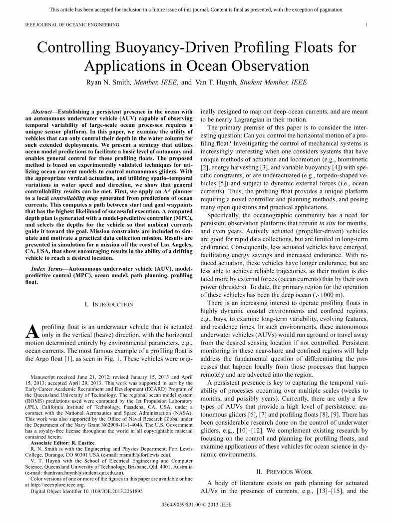
motion determined entirely by environmental parameters, e.g.,ocean currents. The most famous example of a profiling float isthe Argo float [1], as seen in Fig. 1. These vehicles were orig-

Manuscript received June 21, 2012; revised January 15, 2013 and April15, 2013; accepted April 29, 2013. This work was supported in part by theEarly Career Academic Recruitment and Development (ECARD) Program ofthe Queensland University of Technology. The regional ocean model system(ROMS) predictions used were computed by the Jet Propulsion Laboratory(JPL), California Institute of Technology, Pasadena, CA, USA, under acontract with the National Aeronautics and Space Administration (NASA).This work was also supported by the Office of Naval Research Global underthe Department of the Navy Grant N62909-11-1-4046. The U.S. Governmenthas a royalty-free license throughout the world in all copyrightable materialcontained herein.Associate Editor: R. Eustice.R. N. Smith is with the Engineering and Physics Department, Fort Lewis

College, Durango, CO 80301 USA (e-mail: [email protected]).V. T. Huynh with the School of Electrical Engineering and Computer

Science, Queensland University of Technology, Brisbane, Qld. 4001, Australia(e-mail: [email protected]).Color versions of one or more of the figures in this paper are available online

at http://ieeexplore.ieee.org.Digital Object Identifier 10.1109/JOE.2013.2261895

inally designed to map out deep-ocean currents, and are meantto be nearly Lagrangian in their motion.The primary premise of this paper is to consider the inter-

esting question: Can you control the horizontal motion of a pro-filing float? Investigating the control of mechanical systems isincreasingly interesting when one considers systems that haveunique methods of actuation and locomotion (e.g., biomimetic[2], energy harvesting [3], and variable buoyancy [4]) with spe-cific constraints, or are underactuated (e.g., torpedo-shaped ve-hicles [5]) and subject to dynamic external forces (i.e., oceancurrents). Thus, the profiling float provides a unique platformrequiring a novel controller and planning methods, and posingmany open questions and practical applications.Specifically, the oceanographic community has a need for

persistent observation platforms that remain in situ for months,and even years. Actively actuated (propeller-driven) vehiclesare good for rapid data collections, but are limited in long-termendurance. Consequently, less actuated vehicles have emerged,facilitating energy savings and increased endurance. With re-duced actuation, these vehicles have longer endurance, but areless able to achieve reliable trajectories, as their motion is dic-tated more by external forces (ocean currents) than by their ownpower (thrusters). To date, the primary region for the operationof these vehicles has been the deep ocean ( 1000 m).There is an increasing interest to operate profiling floats in

highly dynamic coastal environments and confined regions,e.g., bays, to examine long-term variability, evolving features,and residence times. In such environments, these autonomousunderwater vehicles (AUVs) would run aground or travel awayfrom the desired sensing location if not controlled. Persistentmonitoring in these near-shore and confined regions will helpaddress the fundamental question of differentiating the pro-cesses that happen locally from those processes that happenremotely and are advected into the region.A persistent presence is key to capturing the temporal vari-

ability of processes occurring over multiple scales (weeks tomonths, and possibly years). Currently, there are only a fewtypes of AUVs that provide a high level of persistence: au-tonomous gliders [6], [7] and profiling floats [8], [9]. There hasbeen considerable research done on the control of underwatergliders, e.g., [10]–[12]. We complement existing research byfocusing on the control and planning for profiling floats, andexamine applications of these vehicles for ocean science in dy-namic environments.

II. PREVIOUS WORK

A body of literature exists on path planning for actuatedAUVs in the presence of currents, e.g., [13]–[15], and the

0364-9059/$31.00 © 2013 IEEE


2 IEEE JOURNAL OF OCEANIC ENGINEERING

Fig. 1. Three examples of profiling floats that are currently in operation. (a) AnArgo profiling float manufactured by Teledyne Webb Research, Inc. (Falmouth,MA, USA). (b) The Sounding Oceanographic Lagrangrian Observer ThermalRECharging (SOLO–TREC) profiling float. Credit: The National Aeronauticsand Space Administration (NASA)/Jet Propulsion Laboratory (JPL)/U.S. Navy/Scripps Institution of Oceanography. (c) The University of Rhode Island pro-filing float. Credit: Chris Roman, Graduate School of Oceanography, Universityof Rhode Island.

references contained therein. These studies primarily relate toquasi-steady-state ocean currents without consideration of ve-hicle actuation limits and often not identifying infeasible paths,particularly in strong ocean currents. Additionally, these in-tended applications assume that the AUV maintains a constantdepth. The use of ocean currents to enable minimum-energy,continuous path planning in three spatial dimensions wasproposed in [16]. Here the authors considered vehicle actuationlimits using a multidimensional cost function for generatingenergy and time optimal paths in estuarine environments. Giventhe application domain, the current profile is assumed to bebidirectional and stratified. In an extension of this work, a newoptimal (time and energy) path-planning approach was demon-strated with an actuated AUV in a tidally forced, dynamic bay[17]. This work illustrated the potential to use currents forimproving vehicle range and endurance, as well as waypointcontrol in regions with tidally varying obstacles. Witt et al.[17] also exposed the utility of current variability with respectto depth in path planning for underwater vehicles.Control of profiling floats is an emerging area of study with a

very limited amount of prior investigation. Recent research hasseen profiling floats applied in multiple applications from phys-ical oceanography to underwater imaging, e.g., [9]. Such workhas demonstrated an increased utility for the profiling float, anda need to investigate extending the control capabilities for suchvehicles.There has been analogous work published on the control of

hot air balloons using wind prediction models [18]. In this work,the authors use a Markov decision process for probabilisticmotion planning through arbitrary, uncertain vector fields, withan emphasis on high-level planning to solve a time-optimalproblem. This work builds upon the well-understood problemof planning wind-efficient paths from the aeronautics com-

munity. In the AUV community, theoretical methods havebeen established for controlled Lagrangian particle tracking toanalyze the offsets between physical positions of marine robotsin the ocean and simulated positions of controlled particles inan ocean model [19]. This application considered autonomousgliders, which can apply controls to move horizontally, contraryto the profiling float.The design of an ocean-scale, sensor web was proposed via

intelligent control of deployed Argo floats in [20]. Dahl et al.examined the maximal coverage andmotion toward a goal prob-lems for multiple floating assets. The two algorithms presentedin [20] were a constant depth strategy and a greedy approach tochoosing a depth that used only a single time-step look-aheadin a large-scale ocean model with low spatio–temporal resolu-tion. The model used has a 7-km horizontal resolution, with cur-rents assumed to be constant over each day [21]. The applicationdomain was the deep ocean, with discrete control actions oc-curring on the order of days. In a more dynamic environment,the development of a feedback controller for a single float op-erating in a tidally forced (single direction currents at each timestep) region is presented in [22]. Jouffroy et al. take advantageof a near-zero current at depth and present a unique anchoringmechanism to enable loitering to avoid adverse currents whenthe tide is opposing the direction of desired motion. Thus, theproposed controller selects either the seafloor or the sea surfaceto enable waypoint tracking. The study in [22] was extendedin [23], and provides a sufficient condition for controllabilitygiven three current directions that span the plane. The authorsassume that the three currents can be taken as constant in bothamplitude and direction. The work presented in [22] and [23],along with [24] and [25] is the first example of research into thedevelopment of control strategies for profiling floats to enableoperation in dynamic and constrained coastal environments.In this paper, we extend existing results to develop the tools

that enable persistent monitoring with profiling floats in a dy-namic coastal ocean environment. The five specific contribu-tions of this paper are the following.1) reformulation of the equations of motion for an AUV sub-jected to ocean currents;

2) controllability analysis for a profiling float in a dynamic,coastal environment;

3) derivation of a controllability map for probabilistic pathplanning with a deterministic ocean model;

4) a model-predictive controller (MPC) that computes thecontrol actions (prescribed depth plan) to steer a profilingfloat between two given locations;

5) simulation results validating the proposed method for dif-ferent current regimes within the region of interest.

The reformulation in contribution 1 is an extension of the ini-tial presentation in [24]; this incorporates ocean model predic-tions into the equations of motion in the form of a control input,rather than a drift term or unknown component. The novelty isthat, for the profiling float, we can directly change the effect ofthe ocean current, i.e., we can control it, by altering the depthof the vehicle. The controllability analysis of contribution 2considers these reformulated equations of motion and providesnecessary conditions for controllability of the reformulated dy-namic system. The result provided is analogous to that presented


SMITH AND HUYNH: CONTROLLING BUOYANCY-DRIVEN PROFILING FLOATS FOR APPLICATIONS IN OCEAN OBSERVATION 3

in [23] in that we show the necessity of a spanning set of velocityvectors for controllability. The difference in this paper is that wedo not consider a minimal spanning set, but only require thatthe origin be within the convex hull of the chosen vectors. Ad-ditionally, we assume here that the currents are time varying inboth direction and magnitude. With the necessary conditions forcontrollability, we present a controllability map, which was firstintroduced in [25]. This representation of the controllability of aregion was specifically designed for mission planning of under-actuated vehicles that exploit ocean currents. The map displaysthe current variability with respect to depth, providing a guidefor planning purposes. Profiling floats will be more controllablein regions of more diverse currents, while an AUV with moreactuation may prefer to go through regions of low variabilityto reduce uncertainty. Incorporating ocean model predictions inplanning and control has been shown through field trials to be aneffective method for reducing navigation error due to externaldisturbances for underactuated vehicles [26], [27]. A first ver-sion of the controller in contribution 4 was presented in [25],and is updated here with an examination of the stability and fur-ther validations provided in contribution 5.The outline of the remainder of the paper is as follows. In Sec-

tion III, we present a few examples of existing profiling floats togive a brief description of this unique vehicle. Section IV detailsthe regional ocean modeling system; the predictive ocean modelused in this study. In Section V, we present the standard equa-tions ofmotion for the considered system, and then derive the re-formulated equations based on the assumptions and informationavailable. Given these new equations of motion, we then presentan analysis of the controllability of this dynamic system, andprovide the necessary conditions to achieve the general controlthat we desire. In Section VII, we utilize the oceanmodel and thenecessary conditions to compute the controllability map, whichprovides a measure of expected controllability at each discretelocation in the ocean model. We then apply an A* planner, withthe controllability map providing the underlying cost function,to compute a path connecting any two waypoints that has thehighest expected controllability, and in turn, the greatest prob-ability of successful execution. This path contains intermediatewaypoints that steer the vehicle through highly controllable re-gions between the start and the goal. In Section VIII, we derivean MPC that steers the float along the computed path. The con-troller is designed to prescribe a depth for the float at each hour,so that the ocean currents push it along the path and eventuallyto the goal.We detail the constraints on the controller from a sci-ence-motivated point of view, and provide an examination of thestability and convergence of our proposed system. Section IXpresents data from simulations in a coastal ocean region nearLos Angeles, CA, USA. We conclude with some observationsand present plans for future work and field deployments.

III. PROFILING FLOATS

The vehicles considered here are commonly referred to in theliterature as Lagrangian floats, profiling floats, or Lagrangianprofilers; we use profiling floats. These vehicles have beenutilized in ocean science research for multiple decades; see,e.g., [28]–[31]. We leverage recent advancements in oceanmodeling and forecasting to examine the potential to increase

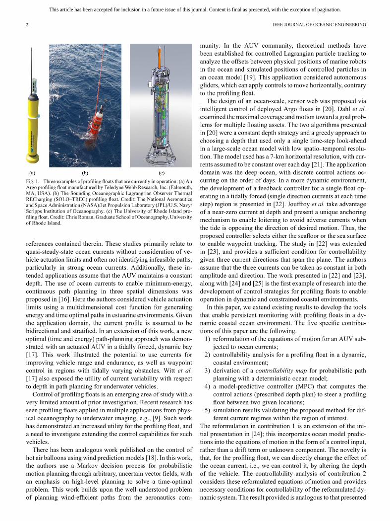
Fig. 2. Current location of Argo floats. Image courtesy of the Argo home page,http://www.argo.ucsd.edu/index.html.

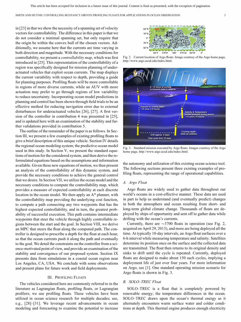
Fig. 3. Standard mission executed by Argo floats. Images courtesy of the Argohome page, http://www.argo.ucsd.edu/index.html.

the autonomy and utilization of this existing ocean science tool.The following sections present three existing examples of pro-filing floats, representing the range of operational capabilities.

A. Argo Float

Argo floats are widely used to gather data throughout ourworld’s oceans in a cost-effective manner. These data are usedin part to help us understand (and eventually predict) changesin both the atmosphere and ocean resulting from short- andlong-term global climate change. Thousands of floats are de-ployed by ships of opportunity and sent off to gather data whiledrifting with the ocean’s currents.Currently, there are 3700 floats in operation (see Fig. 2,

acquired on April 29, 2013), andmore are being deployed all thetime. At typically 10-day intervals, an Argo float surfaces over a6-h interval while measuring temperature and salinity. Satellitesdetermine its position once on the surface and the collected dataare transmitted. The float then returns to its original density andsinks to drift until the cycle is repeated. Currently, deployedfloats are designed to make about 150 such cycles, implying adeployment life of just over four years. For more informationon Argo, see [1]. One standard operating mission scenario forArgo floats is shown in Fig. 3.

B. SOLO–TREC Float

SOLO–TREC is a float that is completely powered byrenewable energy; the temperature differences in the ocean.SOLO–TREC draws upon the ocean’s thermal energy as italternately encounters warm surface water and colder condi-tions at depth. This thermal engine produces enough electricity



to operate the vehicle’s science instruments, Global Posi-tioning System (GPS) receiver, communications device, andbuoyancy-control pump. SOLO–TREC has demonstrated thecapability of continuously executing three to four dives per day[32].

C. University of Rhode Island Float

The previous two profiling float examples provide a high-en-durance platform, however, their operation is restricted to thedeep ocean, i.e., 1000-m depth. For coastal regions, these ve-hicles are not appropriate, which has promoted the developmentof a shallow-water profiling float.The University of Rhode Island (URI, Kingston, RI, USA)

has developed novel floats with an active ballasting system andacoustic altimeters, enabling them to position themselves any-where in the water column, providing the ability to perform arange of drifting and profiling behaviors. These floats are ableto operate successfully in areas of highly varied bathymetry, es-pecially in near-shore environments. The float is built around apiston-style, volume-changing mechanism, allowing the buoy-ancy actuator to achieve profiling speeds of up to 20m/min, withsettling times O(10 s). For further information, see [9].

D. Assumed Float Characteristics

We assume that the vertical position of the float within thewater column can be accurately controlled, albeit limited, andthe horizontal velocity is determined strictly by ocean currents;varying with depth and geographic location. We adopt a simplemodel for the profiling float, assuming that the vehicle motion isconstrained to . Hence, we assume that the float is invariantin roll , pitch , and yaw . We assume that the float isrepresented dynamically as a point mass and can change depthinstantaneously.

IV. OCEAN MODEL INPUT

The predictive tool that we utilize for general open oceancurrents in the pacific basin is the regional ocean model system(ROMS)—a split-explicit, free-surface, topography-fol-lowing-coordinate oceanic model. ROMS is an open-sourceocean model that is widely accepted and supported throughoutthe oceanographic and modeling communities. The modelsolves the primitive equations using the Boussinesq and hy-drostatic approximations in vertical sigma (i.e., topographyfollowing) and horizontal orthogonal curvilinear coordinates.ROMS uses innovative algorithms for advection, mixing,pressure gradient, vertical-mode coupling, time stepping, andparallel efficiency. Detailed information on ROMS can befound in [33] and [34].The ROMS output has three nested horizontal resolutions

covering the U.S. west coastal ocean (15 km), the southern Cal-ifornia coastal ocean (5 km), and the Southern California Bight(SCB; 2.2 km). The three nested ROMS domains are coupledonline and run simultaneously exchanging boundary conditions,ultimately providing hourly hindcasts, nowcasts, and forecasts(up to 72 h) for southern California. The vertical resolution isnonuniform, providing data at 24 discrete depths ranging from0 to 2000 m. Applications of this 4-D model implemented in

AUV path planning can be found in [35], [36], and the refer-ences contained therein.

V. EQUATIONS OF MOTION

Given the assumptions of invariance in roll, pitch, and yaw,we define the three-degree-of-freedom configuration space ofthe float as . We define a body-fixed coordinate frame, located at the point ; the center of gravity (CG)

of the float. We assume that the vehicle can adjust to be neu-trally buoyant at a prescribed depth, and the CG and the centerof buoyancy (CB) are located along the same vertical axis in. The state of the underwater vehicle is given by the vector

and describes the position of the float withrespect to the inertial reference frame. The vertical position ofthe float can be controlled, and the horizontal velocities

are determined strictly by ocean currents. Letrepresent the 4-D ( ; three spatial plus

time) north–south (zonal), east–west (meridional), and verticalcurrents, respectively. Velocity is taken to be positive eastward,northward, and opposing gravity. As the focus of this paper isto utilize the depth variation of the currents at each location, wesuppress the horizontal dimensions for notational convenience.Specifically, given a latitude and longitude [ location], wedefine the ocean currents as functions of only depth and time, . Then, conventionally, we would ex-

press the equations of motion in as

(1)

where represents the input control. In this scenario,corresponds to the chosen depth at a given time .Initially, we ignore vertical currents, i.e., ,

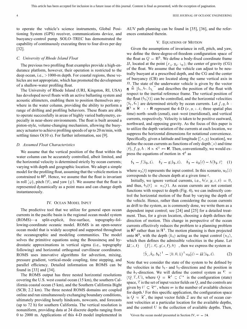
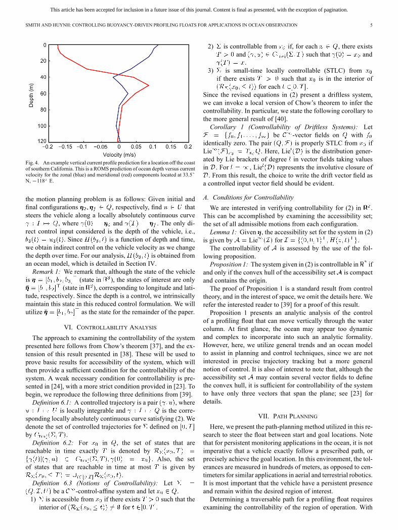
and thus, . As ocean currents are not constantfunctions with respect to depth (Fig. 4), we can indirectly con-trol the horizontal motion of the float by varying the depth ofthe vehicle. Hence, rather than considering the ocean currentsas drift to the system, as is commonly done, we write them as adependent input control; see [24] and [25] for a detailed treat-ment. Thus, for a given location, choosing a depth defines thedirection of motion. This change in perspective of the oceancurrents effectively reduces the problem to a planning problemin rather than in . The motion planning is then projectedonto , with the depth acting as the input control ,which then defines the admissible velocities in the plane. Let

, then we express the system as

(2)

Note that we consider the state of the system to be defined bythe velocities in the - and -directions and the position inthe -direction. We will define the control system as

, where is the configuration (state)space, is the set of input vector fields on , and the controls aregiven by , where is the number of available choicesfor depth.1 For this specific application, the configuration spaceis , the input vector fields are the set of ocean cur-rent velocities at a particular location for the available depths,and the control is the collection of available depths. Then,

1Given the ocean model presented in Section IV, .



Fig. 4. An example vertical current profile prediction for a location off the coastof southern California. This is a ROMS prediction of ocean depth versus currentvelocity for the zonal (blue) and meridional (red) components located at 33.5N, 118 E.

the motion planning problem is as follows: Given initial andfinal configurations , respectively, find thatsteers the vehicle along a locally absolutely continuous curve

, where and . The only di-rect control input considered is the depth of the vehicle, i.e.,

. Since is a function of depth and time,we obtain indirect control on the vehicle velocity as we changethe depth over time. For our analysis, is obtained froman ocean model, which is detailed in Section IV.Remark 1: We remark that, although the state of the vehicle

is (state in ), the states of interest are only(state in ), corresponding to longitude and lati-

tude, respectively. Since the depth is a control, we intrinsicallymaintain this state in this reduced control formulation. We willutilize as the state for the remainder of the paper.

VI. CONTROLLABILITY ANALYSIS

The approach to examining the controllability of the systempresented here follows from Chow’s theorem [37], and the ex-tension of this result presented in [38]. These will be used toprove basic results for accessibility of the system, which willthen provide a sufficient condition for the controllability of thesystem. A weak necessary condition for controllability is pre-sented in [24], with a more strict condition provided in [23]. Tobegin, we reproduce the following three definitions from [39].Definition 6.1: A controlled trajectory is a pair , where

is locally integrable and is the corre-sponding locally absolutely continuous curve satisfying (2). Wedenote the set of controlled trajectories for defined onby .Definition 6.2: For in , the set of states that are

reachable in time exactly is denoted by. Also, the set

of states that are reachable in time at most is given by.

Definition 6.3 (Notions of Controllability): Letbe a -control-affine system and let .

1) is accessible from if there exists such that theinterior of for .

2) is controllable from if, for each , there existsand such that and.

3) is small-time locally controllable (STLC) fromif there exists such that is in the interior of

for each .Since the revised equations in (2) present a driftless system,we can invoke a local version of Chow’s theorem to infer thecontrollability. In particular, we state the following corollary tothe more general result of [40].Corollary 1 (Controllability of Driftless Systems): Let

be -vector fields on withidentically zero. The pair is properly STLC from ifLie . Here, Lie is the distribution gener-ated by Lie brackets of degree in vector fields taking valuesin . For , Lie represents the involutive closure of. From this result, the choice to write the drift vector field as

a controlled input vector field should be evident.

A. Conditions for Controllability

We are interested in verifying controllability for (2) in .This can be accomplished by examining the accessibility set;the set of all admissible motions from each configuration.Lemma 1: Given , the accessibility set for the system in (2)

is given by Lie for .The controllability of is assessed by the use of the fol-

lowing proposition.Proposition 1: The system given in (2) is controllable in if

and only if the convex hull of the accessibility set is compactand contains the origin.The proof of Proposition 1 is a standard result from control

theory, and in the interest of space, we omit the details here. Werefer the interested reader to [39] for a proof of this result.Proposition 1 presents an analytic analysis of the control

of a profiling float that can move vertically through the watercolumn. At first glance, the ocean may appear too dynamicand complex to incorporate into such an analytic formality.However, here, we utilize general trends and an ocean modelto assist in planning and control techniques, since we are notinterested in precise trajectory tracking but a more generalnotion of control. It is also of interest to note that, although theaccessibility set may contain several vector fields to definethe convex hull, it is sufficient for controllability of the systemto have only three vectors that span the plane; see [23] fordetails.

VII. PATH PLANNING

Here, we present the path-planning method utilized in this re-search to steer the float between start and goal locations. Notethat for persistent monitoring applications in the ocean, it is notimperative that a vehicle exactly follow a prescribed path, orprecisely achieve the goal location. In this environment, the tol-erances are measured in hundreds of meters, as opposed to cen-timeters for similar applications in aerial and terrestrial robotics.It is most important that the vehicle have a persistent presenceand remain within the desired region of interest.Determining a traversable path for a profiling float requires

examining the controllability of the region of operation. With



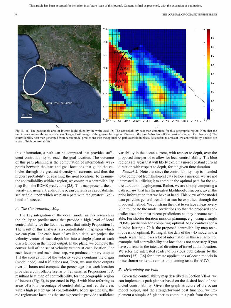
Fig. 5. (a) The geographic area of interest highlighted by the white oval. (b) The controllability heat map computed for this geographic region. Note that thetwo images are not the same scale. (a) Google Earth image of the geographic region of interest; the San Pedro Bay off the coast of southern California. (b) Thecontrollability heat map generated from ocean model predictions with the optimal A* path overlaid in black. Blue refers to areas of low controllability, and red areareas of high controllability.

this information, a path can be computed that provides suffi-cient controllability to reach the goal location. The outcomeof this path planning is the computation of intermediate way-points between the start and goal locations that guide the ve-hicles through the greatest diversity of currents, and thus thehighest probability of reaching the goal location. To examinethe controllability within a region, we construct a controllabilitymap from the ROMS predictions [25]. This map presents the di-versity and general trends of the ocean currents as a probabilisticscalar field, upon which we plan a path with the greatest likeli-hood of success.

A. The Controllability Map

The key integration of the ocean model in this research isthe ability to predict areas that provide a high level of localcontrollability for the float, i.e., areas that satisfy Proposition 1.The result of this analysis is a controllability map upon whichwe can plan. For each hour of available data, we project thevelocity vector of each depth bin into a single plane at eachdiscrete node in the model output. In the plane, we compute theconvex hull of the set of velocity vectors at each location. Foreach location and each time step, we produce a binary output;1 if the convex hull of the velocity vectors contains the origin(model node), and 0 if it does not. Then, we sum these outputsover all hours and compute the percentage that each locationprovides a controllable scenario, i.e., satisfies Proposition 1. Aresultant heat map of controllability, for the geographic regionof interest (Fig. 5), is presented in Fig. 5 with blue referring toareas of a low percentage of controllability, and red the areaswith a high percentage of controllability. More specifically, thered regions are locations that are expected to provide a sufficient

variability in the ocean current, with respect to depth, over theproposed time period to allow for local controllability. The blueregions are areas that will likely exhibit a more constant currentdirection with respect to depth, for the given time duration.Remark 2: Note that since the controllability map is intended

to be computed from historical data before a mission, we are notinterested in utilizing it to compute the optimal path for the en-tire duration of deployment. Rather, we are simply computing apath a priori that has the greatest likelihood of success, given theprior information that we have at hand. This view of the modeldata provides general trends that can be exploited through theproposed method.We constrain the float to surface at least every70 h to update the model predictions so that the proposed con-troller uses the most recent predictions as they become avail-able. For shorter duration mission planning, e.g., using a singleROMS prediction for computing optimal AUV controls for amission lasting 70 h, the proposed controllability map tech-nique is not optimal. Rolling all the data of the 4-D model into asingle scalar field loses a lot of information in this scenario. Forexample, full controllability at a location is not necessary if youhave currents in the intended direction of travel at that location.We refer the interested reader to previous publications by theauthors [35], [36] for alternate applications of ocean models inthese shorter or iterative mission planning tasks for AUVs.

B. Determining the Path

Given the controllability map described in Section VII-A, wecan implement a path planner based on the desired level of pre-dicted controllability. Given the graph structure of the oceanmodel output, and the straightforward cost function, we im-plement a simple A* planner to compute a path from the start



location to the goal. This produces intermediate waypoints atdiscrete locations that correspond with the nodes in the oceanmodel output. The optimization constraint considered is to min-imize the cost function over the path between thestart and the goal, where is the percentage of controllabilityat a given node. The path computed by the A* planner will, ingeneral, be different than the straight line path connecting thestart and goal waypoints since it guides the float through areasof maximal controllability.A path planned by this method is given by the black line

in Fig. 5 on an example controllability map. The start locationis just off the tip of Catalina Island, CA, USA, and is labeledSTART and is depicted by a white dot in Fig. 5. The end of thepath is labeled END, and is given by the black dot and is locatedjust off the California coast. The four dots (WP1, WP2, WP3,and WP4) along the path are intermediate waypoints computedby the A* planner.Remark 3: For practical reasons, we cannot assume to know

or have a prediction of the ocean currents a priori for the en-tire duration of a long-term deployment (weeks to months). TheROMS used here only provides a 72-h forecast, which is insuffi-cient for preplanning even a week-long mission. To circumventthis, we rely on regional trends in the structure of ocean cur-rents within a specific area of interest. Specifically, in the chosenarea of interest, there are three distinct seasons when consid-ering ocean dynamics: an upwelling season fromMarch throughMay and partially into June, the summer/early fall season runsfrom mid-June into October, and the transition season that oc-curs from November through February. During each season, wecan assume a similar current structure to persist. For example,from June to October, the average flow tends to be downcoast(southerly), while from November to March, the average flowtends to be upcoast (nortward) [41], [42]. To this end, the pro-posed planning methodology is designed to generate the con-trollability map based on a set of historical model predictions(approximately two weeks for the presented simulations), plana path for the highest likelihood of success on this map, then ex-ecute this path based upon model updates as they become avail-able in real time. Hence, although the presented results are simu-lations, they were conducted as if the float were operating in theocean. In Section VIII, we provide constraints on the controllerto adequately account for need to update current predictions asthey become available.

VIII. CONTROL STRATEGY

The chosen mission is to persistently execute a transectcrossing the channel between the U.S. west coast and CatalinaIsland, as highlighted in Fig. 5. The mission is scientificallymotivated by a desire to understand the nutrient flux within theSan Pedro Bay. Given this science motivation and the ROMSoutput, we impose the following operational constraints uponour controller.• ROMS provides 72-h predictions each day, thus we fix amaximum of 70 h between surfacings.

• For safety, we neither want to surface frequently nor stayon the surface for extended periods of time. Thus, we set aminimum 6-h limit between surfacings, and only allow thefloat to remain on the surface for 1 h.

• Motivated by the underlying science, we require the floatto perform periodic, full-depth, vertical profiles. This isimplemented by requiring the float to go to the seafloor (ormaximum prescribed depth) for the time-step immediatelypreceding a scheduled surfacing.

• We do not constrain the float to follow a prescribed tra-jectory, but provide control such that each waypoint isachieved to within a user-defined tolerance .

We base the controller design on the equations of motion de-rived previously. In Sections V and VI, we present an analyticrepresentation for the system and the controllability. Given thatthe ROMS output is discrete in time, the input to the controllerwill not change over a single time epoch (for ROMS, this is1 h), and hence, a computed control action would remain con-stant over that time period. Additionally, energy consumption onthis type of vehicle directly corresponds to changes in buoyancy(depth), and reducing these changes increases the deploymenttime, giving a more persistent presence. Thus, we are motivatedto consider a discrete-time controller for this application.To convert from the continuous equations to the discrete-time

application, we define the following variables. Let the state ofthe system be defined by , and the systemoutput be defined by . Since the ROMS output con-tains 24 discrete depths, is the set of inputcontrol vectors, where with thenonzero entry as the th component of the vector. Hence, thecontrol input is bang–bang, and we interpret that a control ofcommands the float to the sea surface, while a control of

for commands the float to the associated depthwithin the ROMS output discretization. Function in (1)is then a piecewise constant function of the assigned depths forthe float, and we let represent the discrete-time control inputto the system. Since the ocean is not always 2000 m deep (max-imum ROMS depth, ) in the operational region, or inthe event that we would like to limit the operational depth ofthe vehicle within the controller, we allow for

, where is the maximum ocean depth allowed for agiven location. For the examples presented here, we set a max-imum depth of 1000 m, corresponding to , althoughthe actual depth at a location may be less than this in many in-stances.We choose to implement a robust constrained finite horizon

model-predictive controller (RCFMPC). We assume that thereare no sudden changes in the velocity of the ocean currents withrespect to time. Given the system parameters defined above, wewrite a discrete-time, linear time-varying (LTV) system as fol-lows:

(3)

(4)

Here, is the 2 2 identity matrix. Matrix is a 2 24matrix giving the and velocities at each depth at locationfrom the ROMSmodel. This matrix is obtained by interpolatinga set consisting of four similar matrices output from ROMS;one matrix for each discrete ROMS grid point that defines thebounding box around the current location of the float. The setacts as a lookup table for the predicted currents at a given



spatio–temporal location, and is taken from the 7826 total, dis-crete nodes in the ROMS output. Matrix .Let refer to the current time step, define the

finite control horizon, and define the finite pre-diction horizon. Let be the control action at time ,given we are at time . We assume that there is no control actionafter time , i.e., . From the modelin (3), the RCFMPC has the following objective:

(5)

where

(6)

Here, and are symmetric, positive–definite,weighting matrices, and is the finite horizon, or number oflook-ahead steps. From (3) and (6), note that is a functionof both and , although we suppress this notationhere. Set is the set of possible matrices for . Since wecompute as an interpolation of the ROMS output, thereis an inherent uncertainty in this computation. We allow tohave finitely many values to incorporate this uncertainty intothe controller.Since and are positive definite, (5) is equivalent to

minimizing the objective (distance between the current state andthe goal) at each step of the prediction horizon ,with the largest (worst case) value of , as shown in

(7)The desired RCFMPC is subject to the following constraints.• Output

for (8)

Since the destination waypoint is chosen to be the origin,we always have the final state approaching zero.

• Input

(9)

• Acceptable current directions: Let ,, and be an angle about the azimuth

from the current location of the vehicle to the prescribedwaypoint that defines a range for acceptable ocean currentsto choose. This gives the following constraint:

(10)

• Terminal

(11)

where is a ball of radius that is a user-defined param-eter for the control algorithm.

We impose the angle of acceptable current constraint in (10)to ensure that the velocity vector at a chosen depth generally

points toward the destination waypoint. This constraint reducesthe number of depth choices to only those that provide a cur-rent that reduces the distance to the goal at each time step. Theimplementation of this constraint was motivated by [22], wherethe guiding angle constraint is defined as a symmetric sectorof sight about the line of sight between the actual position ofthe vehicle and the destination point. It is worth noting that theguiding angle constraint in (10) is not necessary, but imposed tospeed up the convergence of the RCFMPC. Eliminating or re-laxing this constraint could result in a movement that increasesthe distance to the goal for a given time step. This scenario ismuch more flexible for execution, but requires onboard recom-putation of the path at each stage to ensure that the vehicle doesnot diverge into a region where it cannot escape.Remark 4: Observing the objective equation (5) with con-

straint equations (8)–(11), we remark that the RCFMPC is a hy-brid, nonlinear problem. There is no direct method to solve thisproblem explicitly. In our approach, we take advantage of theconstraint equation (9), noting that is a finite set with deter-ministic values. As a result, the RCFMPC is feasible by onlyallowing a finite set of values for the control input. Addition-ally, we utilize the fact that near-zero currents exist at depth(near the seafloor) and possibly other depths within the watercolumn. The vehicle can thus prescribe a depth with little to nocurrent, implying minimal deviation from its path, to wait formore favorable currents to become available in the future. Thistakes advantage of the dynamic nature of the spatio–temporalvariability of ocean currents, and that the path was planned bythe use of the controllability map to be through an area of highcurrent diversity, to provide a solution to the control problem.

A. Stability and Convergence

Having defined the RCFMPC for a profiling float, we nowexamine the stability of this system in the context of the appli-cation. Given that represents a discrete and deterministicprediction of the ocean currents, and the chosen controlis bang–bang, we cannot expect to provide strict guarantees onthe rate or accuracy of convergence of the proposed controller.However, the considered vehicle does not require such guaran-tees and precise control for operation, but rather a broad notionof movement in a given direction or toward a chosen location.By using the controllability map presented in Section VII-A,we can compute a path connecting any two locations that hasthe highest probability of finding a control (ocean current) inthe prescribed direction at each time epoch (each hour). Addi-tionally, as the proposed application is intended to maintain apersistent presence in the ocean, the time constraint is the de-ployment life of the vehicle. Hence, in the context of the pro-posed application, we are interested in asymptotic convergence

to a region . Since the authors work closely withthe developers of the ocean model utilized here, one intent ofthis research is to develop a continuous feedback between thevehicle and the ocean model during field trials. As the motionof the vehicle is purely based on currents, assimilating the de-ployment data will increase the accuracy of future predictions,and in turn, improve the rate and accuracy of convergence of theRCFMPC.



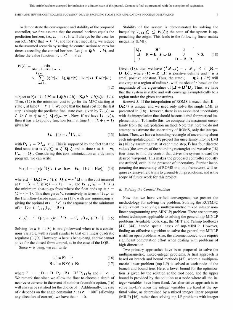
To demonstrate the convergence and stability of the proposedcontroller, we first assume that the control horizon equals theprediction horizon, i.e., . It will always be the case forour RCFMPC that , and for strict inequality, we reduceto the assumed scenario by setting the control actions to zero fortimes exceeding the control horizon. Let , anddefine the value function as

(12)

subject to .Then, (12) is the minimum cost-to-go for the MPC starting atstate at time . We note that the final cost for the laststep is simply the predicted final state cost, given by

. Now, if we have ,then it has a Lyapunov function form at timegiven by

(13)

with . This is supported by the fact that thefinal state cost is , and at time ,

. Considering this cost minimization as a dynamicprogram, we can write

(14)

where , is the cost incurredat if , and isthe minimum cost-to-go from where the float ends up at

. This then gives recursively in terms of asthe Hamilton–Jacobi equation in (15), with any minimizinggiving the optimal as the argument of the minimumof

(15)

Solving for is straightforward when is a contin-uous variable, with a result similar to that of a linear quadraticregulator (LQR). However, here is bang–bang, and we cannotsolve for the closed-form control, as in the case of the LQR.Since is bang, we can write

(16)

(17)

where and .We remark that since we allow the float to choose a depth ofnear-zero currents in the event of no other favorable option, (16)will always be satisfied for the choice of . Additionally, the sizeof depends on the angle constraint ; as 180 (allowingany direction of current), we have that .

Stability of the system is demonstrated by solving theinequality ; the state of the system is ap-proaching the origin. This leads to the following linear matrixinequality (LMI):

(18)

Given (18), then we have, where is positive definite and is a

small positive constant. Thus, the state willconverge to a region of radius , with the size of based on themagnitude of the eigenvalues of . Thus, we havethat the system is stable and will converge asymptotically to aregion under the given constraints.Remark 5: If the interpolation of ROMS is exact, then

is unique, and we need only solve the single LMI, aspresented in (18). However, there is an associated uncertaintywith the interpolation that should be considered for practical im-plementation. To handle this, we compute the maximum uncer-tainty from the interpolation method. Note that here we do notattempt to estimate the uncertainty of ROMS, only the interpo-lation. Then, we have a bounding rectangle of uncertainty abouteach interpolated point.We project this uncertainty into the LMIin (18) by assuming that, at each time step, has four discretevalues (the corners of the bounding rectangle) and we solve (18)four times to find the control that drives the system toward thedesired waypoint. This makes the proposed controller robustlyconstrained, even in the presence of uncertainty. Further incor-porating the uncertainty of ROMS into this framework will re-quire extensive field trials to ground-truth predictions, and is thescope of future work for this project.

B. Solving the Control Problem

Now that we have verified convergence, we present themethodology for solving the problem. Solving the RCFMPCis equivalent to solving a multiparametric mixed integer non-linear programming (mp-MINLP) problem. There are not manyrobust techniques applicable to solving the general mp-MINLPproblems. Available tools, e.g., the MPT and Yalmip toolboxes[43], [44], handle special cases of mp-MINLP. However,finding an effective algorithm to solve the general mp-MINLPis still an open problem. Also, the aforementioned tools requiresignificant computation effort when dealing with problems ofhigh dimension.Two primary approaches have been proposed to solve the

multiparametric, mixed-integer problems. A first approach isbased on branch and bound methods [45], where a multipara-metric linear problem (mp-LP) is solved at each node of thebranch and bound tree. Here, a lower bound for the optimiza-tion is given by the solution at the root node, and the upperbound is provided by the solution at a node where all the in-teger variables have been fixed. An alternative approach is tosolve mp-LPs when the integer variables are fixed at the op-timal value, as determined by a mixed integer linear program(MILP) [46], rather than solving mp-LP problems with integer



variables relaxed in the interval . Both of these methods re-quire significant computation effort, as the search tree expandsnonlinearly with respect to the dimension of the state variables.Motivated by [47], we initially implemented an algorithm basedon greedy, depth-first search [25]. Algorithm 1 is an extensionto our previous work that includes the full vertical profile con-straint mentioned at the beginning of Section VIII. The detailsof incorporating a feedback loop for our controller are given inSection VIII-C.

C. A Closed-Loop Solution

Given the reduced controllability of the profiling float andthe nature of ocean currents, it is foreseeable that the vehiclewill diverge from the prescribed path, even with the proposedRCFMPC. Potential scenarios for such an occurrence may in-clude a poor prediction by ROMS, or a significant time navi-

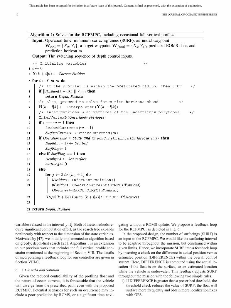
gating without a ROMS update. We propose a feedback loopfor the RCFMPC, as depicted in Fig. 6.In the proposed design, the number of surfacings (SURF) is

an input to the RCFMPC. We would like the surfacing intervalto be adaptive throughout the mission, but constrained withingiven limits. Hence, we incorporate SURF into a feedback loopby inserting a check on the difference in actual position versusestimated position (DIFFERENCE) within the overall controlsystem. Here, DIFFERENCE is computed using the actual lo-cation if the float is on the surface, or an estimated locationwhile the vehicle is underwater. This feedback adjusts SURFthroughout the mission with the following two simple rules.1) If DIFFERENCE is greater than a prescribed threshold, thethreshold check reduces the value of SURF; the float willsurface more frequently and obtain more localization fixeswith GPS.



Fig. 6. Feedback of the surfacing signal (SURF) to form a closed-loop system.

2) If DIFFERENCE is less than a prescribed threshold, thethreshold check makes the value of SURF larger; the floatwill surface less often. This feature prevents a high fre-quency of surfacings, e.g., every hour.

The parameter SURF is bounded both above and below,hence we avoid the following: 1) the float surfaces every hourto obtain a new prediction; and 2) the float never surfacesto update the ROMS. This is implemented via a saturationfunction augmented into the closed-loop system in Fig. 6.

IX. SIMULATION RESULTS

We present three results of the application of the proposedRCFMPC in a simulated scenario to steer a profiling float be-tween two given waypoints. For each example, we set the radiusof the ball to 350 m. This choice of was motivated by

the analysis of vehicle navigation in the deployment region pre-sented in [26] and [27], and iteratively updated through multiplesimulation trials. As shown in Section VIII-A, the selection ofdepends on the form of the matrix ; the ocean model predic-tions. This directly correlates to the magnitude of the ambientcurrents, distance between waypoints along the prescribed path,and resolution of the underlying ocean model. Additionally, thesize of will depend on the trust in the model predictions, sinceeven if the optimal is chosen based on the aforementioned pa-rameters, it is only optimal if the prediction matches reality. Adetailed analysis on the choice of is out of scope of this pre-sentation, but is the subject of ongoing research.

A. Scenario 1: Initial Test

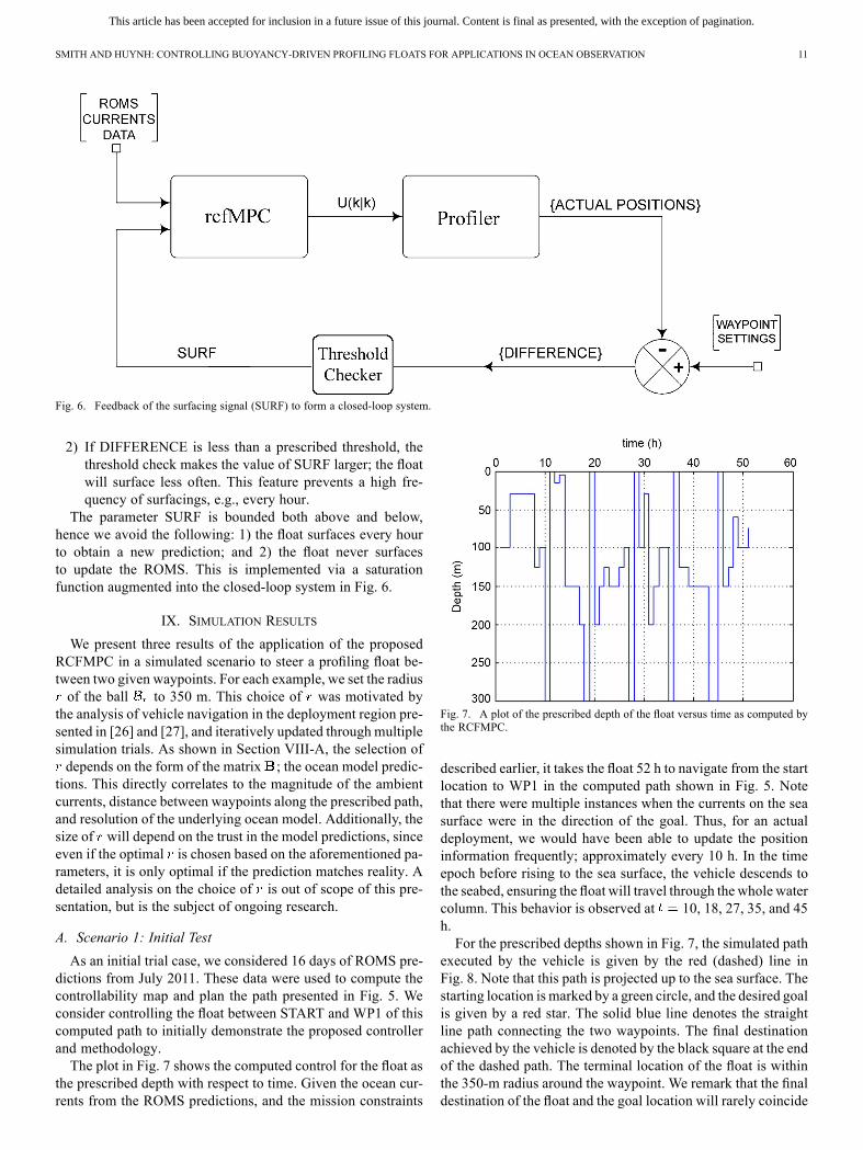
As an initial trial case, we considered 16 days of ROMS pre-dictions from July 2011. These data were used to compute thecontrollability map and plan the path presented in Fig. 5. Weconsider controlling the float between START and WP1 of thiscomputed path to initially demonstrate the proposed controllerand methodology.The plot in Fig. 7 shows the computed control for the float as

the prescribed depth with respect to time. Given the ocean cur-rents from the ROMS predictions, and the mission constraints

Fig. 7. A plot of the prescribed depth of the float versus time as computed bythe RCFMPC.

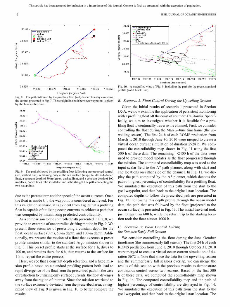
described earlier, it takes the float 52 h to navigate from the startlocation to WP1 in the computed path shown in Fig. 5. Notethat there were multiple instances when the currents on the seasurface were in the direction of the goal. Thus, for an actualdeployment, we would have been able to update the positioninformation frequently; approximately every 10 h. In the timeepoch before rising to the sea surface, the vehicle descends tothe seabed, ensuring the float will travel through the whole watercolumn. This behavior is observed at 10, 18, 27, 35, and 45h.For the prescribed depths shown in Fig. 7, the simulated path

executed by the vehicle is given by the red (dashed) line inFig. 8. Note that this path is projected up to the sea surface. Thestarting location is marked by a green circle, and the desired goalis given by a red star. The solid blue line denotes the straightline path connecting the two waypoints. The final destinationachieved by the vehicle is denoted by the black square at the endof the dashed path. The terminal location of the float is withinthe 350-m radius around the waypoint. We remark that the finaldestination of the float and the goal location will rarely coincide



Fig. 8. The path followed by the profiling float (red, dashed line) by executingthe control presented in Fig. 7. The straight line path between waypoints is givenby the blue (solid) line.

Fig. 9. The path followed by the profiling float following our proposed control(red, dashed line), remaining only at the sea surface (magenta, dashed–dottedline), a constant depth of 50 m (green, dashed line), and a constant depth of 100m (black, dotted line). The solid blue line is the straight line path connecting thetwo waypoints.

due to the parameter and the speed of the ocean currents. Oncethe float is inside , the waypoint is considered achieved. Forthis validation scenario, it is evident from Fig. 8 that a profilingfloat is capable of utilizing ocean currents to achieve a path thatwas computed by maximizing predicted controllability.As a comparison to the controlled path presented in Fig. 8, we

provide an example of uncontrolled driftingmotion in Fig. 9.Wepresent three scenarios of prescribing a constant depth for thefloat: ocean surface (0 m), 50-m depth, and 100-m depth. Addi-tionally, we present the motion of a float that executes a presetprofile mission similar to the standard Argo mission shown inFig. 3. This preset profile starts at the surface for 1 h, dives to100 m, and remains there for 6 h, then returns to the surface for1 h to repeat the entire process.Here, we see that a constant depth selection, and a fixed mis-

sion profile based on a standard profiling pattern both lead torapid divergence of the float from the prescribed path. In the caseof restriction to utilizing only surface currents, the float divergesaway from the region of interest. Since the mission restricted tothe surface extremely deviated from the prescribed area, a mag-nified view of Fig. 9 is given in Fig. 10 to better compare theresults.

Fig. 10. A magnified view of Fig. 9, including the path for the preset standardprofile (solid black line).

B. Scenario 2: Float Control During the Upwelling Season

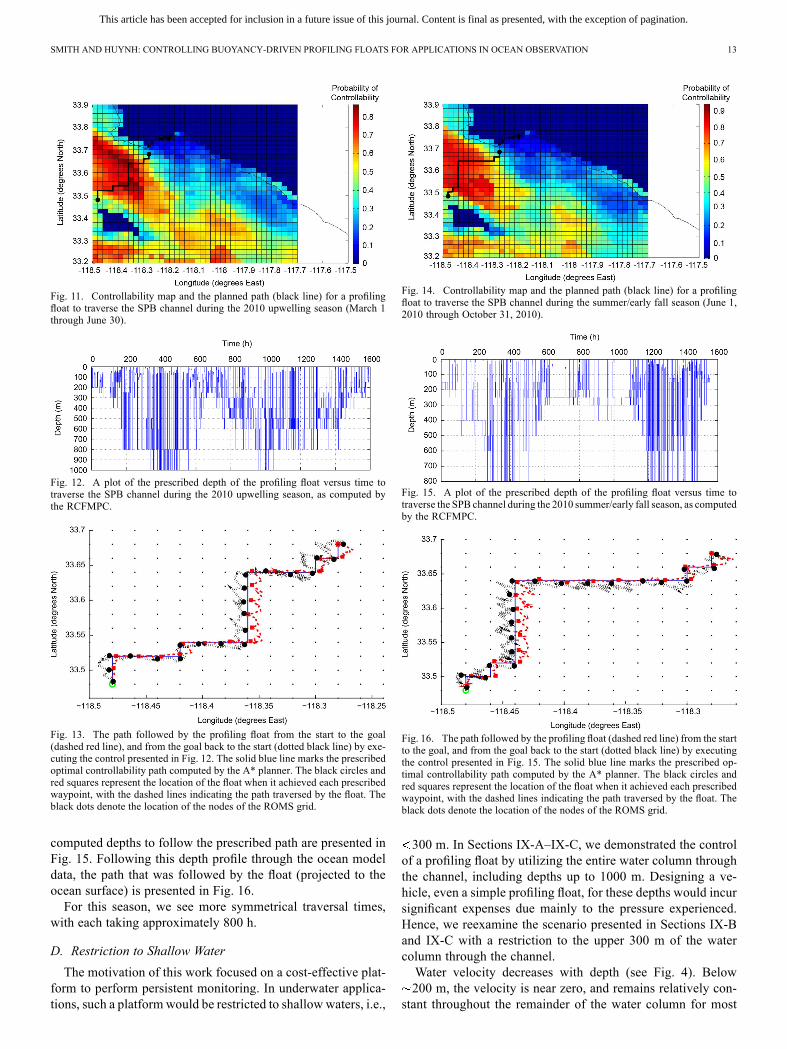
Given the initial results of scenario 1 presented in SectionIX-A, we now examine the application of persistent monitoringwith a profiling float off the coast of southern California. Specif-ically, we aim to investigate whether it is feasible for a pro-filing float to continually traverse the channel. First, we considercontrolling the float during the March–June timeframe (the up-welling season). The first 24 h of each ROMS prediction fromMarch 1, 2010 through June 30, 2010 were merged to create avirtual ocean current simulation of duration 2928 h. We com-puted the controllability map shown in Fig. 11 using the first500 h of these data. The remaining 2400 h of the data wereused to provide model updates as the float progressed throughthe mission. The computed controllability map was used as theinput scalar field to the A* path planner, along with start andend locations on either side of the channel. In Fig. 11, we dis-play the path computed by the A* planner, which denotes thepath of highest percentage of controllability for a profiling float.We simulated the execution of this path from the start to thegoal waypoint, and then back to the original start location. Thecomputed depths to follow the prescribed path are presented inFig. 12. Following this depth profile through the ocean modeldata, the path that was followed by the float (projected to theocean surface) is presented in Fig. 13. The initial traversal tookjust longer than 600 h, while the return trip to the starting loca-tion took the float almost 1000 h.

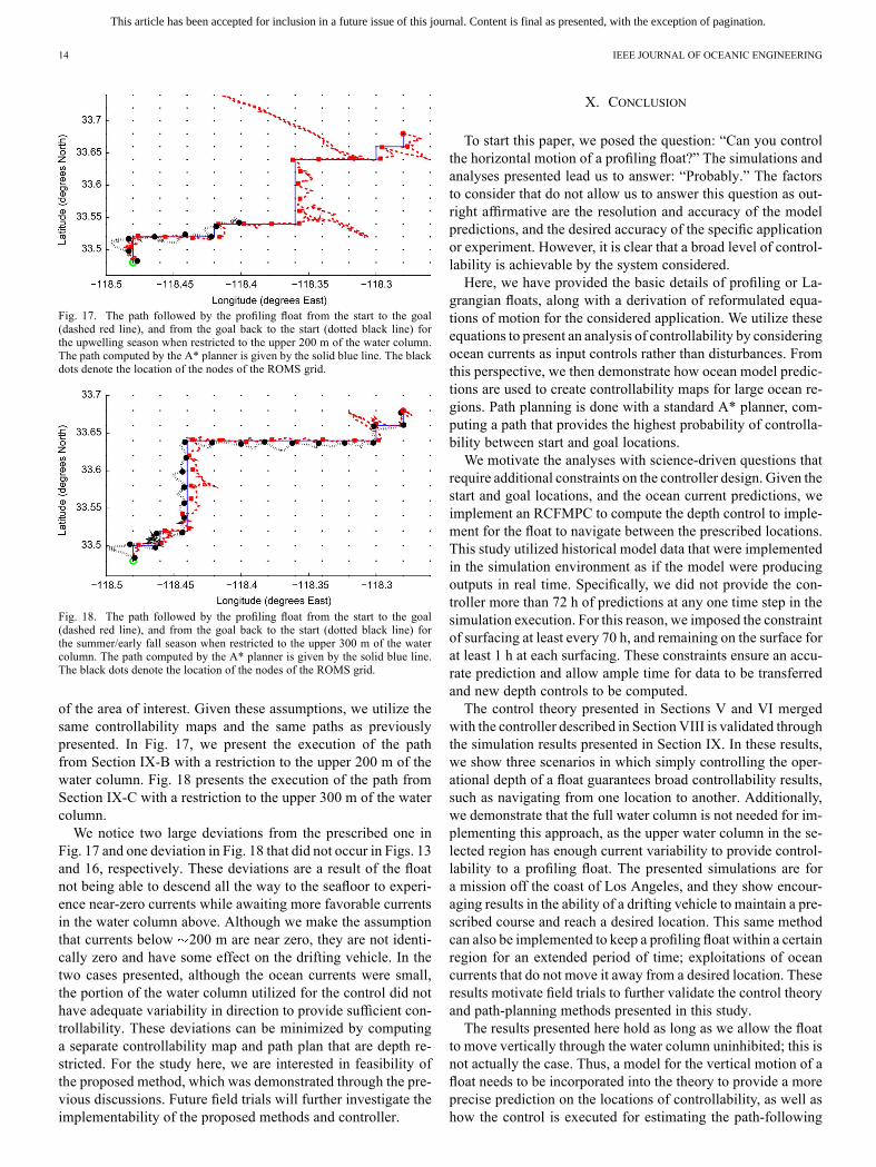
C. Scenario 3: Float Control Duringthe Summer/Early Fall Season

We consider controlling the float during the June–Octobertimeframe (the summer/early fall season). The first 24 h of eachROMS prediction from June 1, 2010 through October 31, 2010were merged to create a virtual ocean current simulation of du-ration 3672 h. Note that since the data for the upwelling seasonand the summer/early fall seasons overlap, we can merge theresults of this section with the previous results to demonstratecontinuous control across two seasons. Based on the first 500h of these data, we computed the controllability map shownin Fig. 14. The computed controllability map and the path ofhighest percentage of controllability are displayed in Fig. 14.We simulated the execution of this path from the start to thegoal waypoint, and then back to the original start location. The



Fig. 11. Controllability map and the planned path (black line) for a profilingfloat to traverse the SPB channel during the 2010 upwelling season (March 1through June 30).

Fig. 12. A plot of the prescribed depth of the profiling float versus time totraverse the SPB channel during the 2010 upwelling season, as computed bythe RCFMPC.

Fig. 13. The path followed by the profiling float from the start to the goal(dashed red line), and from the goal back to the start (dotted black line) by exe-cuting the control presented in Fig. 12. The solid blue line marks the prescribedoptimal controllability path computed by the A* planner. The black circles andred squares represent the location of the float when it achieved each prescribedwaypoint, with the dashed lines indicating the path traversed by the float. Theblack dots denote the location of the nodes of the ROMS grid.

computed depths to follow the prescribed path are presented inFig. 15. Following this depth profile through the ocean modeldata, the path that was followed by the float (projected to theocean surface) is presented in Fig. 16.For this season, we see more symmetrical traversal times,

with each taking approximately 800 h.

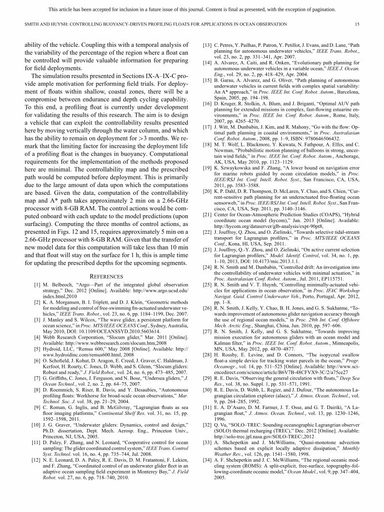
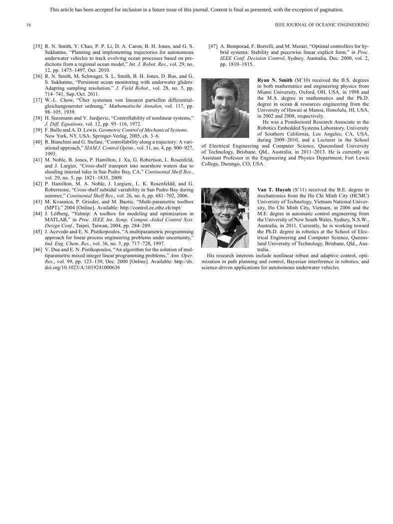
D. Restriction to Shallow Water

The motivation of this work focused on a cost-effective plat-form to perform persistent monitoring. In underwater applica-tions, such a platform would be restricted to shallow waters, i.e.,

Fig. 14. Controllability map and the planned path (black line) for a profilingfloat to traverse the SPB channel during the summer/early fall season (June 1,2010 through October 31, 2010).

Fig. 15. A plot of the prescribed depth of the profiling float versus time totraverse the SPB channel during the 2010 summer/early fall season, as computedby the RCFMPC.

Fig. 16. The path followed by the profiling float (dashed red line) from the startto the goal, and from the goal back to the start (dotted black line) by executingthe control presented in Fig. 15. The solid blue line marks the prescribed op-timal controllability path computed by the A* planner. The black circles andred squares represent the location of the float when it achieved each prescribedwaypoint, with the dashed lines indicating the path traversed by the float. Theblack dots denote the location of the nodes of the ROMS grid.

300 m. In Sections IX-A–IX-C, we demonstrated the controlof a profiling float by utilizing the entire water column throughthe channel, including depths up to 1000 m. Designing a ve-hicle, even a simple profiling float, for these depths would incursignificant expenses due mainly to the pressure experienced.Hence, we reexamine the scenario presented in Sections IX-Band IX-C with a restriction to the upper 300 m of the watercolumn through the channel.Water velocity decreases with depth (see Fig. 4). Below200 m, the velocity is near zero, and remains relatively con-

stant throughout the remainder of the water column for most



Fig. 17. The path followed by the profiling float from the start to the goal(dashed red line), and from the goal back to the start (dotted black line) forthe upwelling season when restricted to the upper 200 m of the water column.The path computed by the A* planner is given by the solid blue line. The blackdots denote the location of the nodes of the ROMS grid.

Fig. 18. The path followed by the profiling float from the start to the goal(dashed red line), and from the goal back to the start (dotted black line) forthe summer/early fall season when restricted to the upper 300 m of the watercolumn. The path computed by the A* planner is given by the solid blue line.The black dots denote the location of the nodes of the ROMS grid.

of the area of interest. Given these assumptions, we utilize thesame controllability maps and the same paths as previouslypresented. In Fig. 17, we present the execution of the pathfrom Section IX-B with a restriction to the upper 200 m of thewater column. Fig. 18 presents the execution of the path fromSection IX-C with a restriction to the upper 300 m of the watercolumn.We notice two large deviations from the prescribed one in

Fig. 17 and one deviation in Fig. 18 that did not occur in Figs. 13and 16, respectively. These deviations are a result of the floatnot being able to descend all the way to the seafloor to experi-ence near-zero currents while awaiting more favorable currentsin the water column above. Although we make the assumptionthat currents below 200 m are near zero, they are not identi-cally zero and have some effect on the drifting vehicle. In thetwo cases presented, although the ocean currents were small,the portion of the water column utilized for the control did nothave adequate variability in direction to provide sufficient con-trollability. These deviations can be minimized by computinga separate controllability map and path plan that are depth re-stricted. For the study here, we are interested in feasibility ofthe proposed method, which was demonstrated through the pre-vious discussions. Future field trials will further investigate theimplementability of the proposed methods and controller.

X. CONCLUSION

To start this paper, we posed the question: “Can you controlthe horizontal motion of a profiling float?” The simulations andanalyses presented lead us to answer: “Probably.” The factorsto consider that do not allow us to answer this question as out-right affirmative are the resolution and accuracy of the modelpredictions, and the desired accuracy of the specific applicationor experiment. However, it is clear that a broad level of control-lability is achievable by the system considered.Here, we have provided the basic details of profiling or La-

grangian floats, along with a derivation of reformulated equa-tions of motion for the considered application. We utilize theseequations to present an analysis of controllability by consideringocean currents as input controls rather than disturbances. Fromthis perspective, we then demonstrate how ocean model predic-tions are used to create controllability maps for large ocean re-gions. Path planning is done with a standard A* planner, com-puting a path that provides the highest probability of controlla-bility between start and goal locations.We motivate the analyses with science-driven questions that

require additional constraints on the controller design. Given thestart and goal locations, and the ocean current predictions, weimplement an RCFMPC to compute the depth control to imple-ment for the float to navigate between the prescribed locations.This study utilized historical model data that were implementedin the simulation environment as if the model were producingoutputs in real time. Specifically, we did not provide the con-troller more than 72 h of predictions at any one time step in thesimulation execution. For this reason, we imposed the constraintof surfacing at least every 70 h, and remaining on the surface forat least 1 h at each surfacing. These constraints ensure an accu-rate prediction and allow ample time for data to be transferredand new depth controls to be computed.The control theory presented in Sections V and VI merged

with the controller described in Section VIII is validated throughthe simulation results presented in Section IX. In these results,we show three scenarios in which simply controlling the oper-ational depth of a float guarantees broad controllability results,such as navigating from one location to another. Additionally,we demonstrate that the full water column is not needed for im-plementing this approach, as the upper water column in the se-lected region has enough current variability to provide control-lability to a profiling float. The presented simulations are fora mission off the coast of Los Angeles, and they show encour-aging results in the ability of a drifting vehicle to maintain a pre-scribed course and reach a desired location. This same methodcan also be implemented to keep a profiling float within a certainregion for an extended period of time; exploitations of oceancurrents that do not move it away from a desired location. Theseresults motivate field trials to further validate the control theoryand path-planning methods presented in this study.The results presented here hold as long as we allow the float

to move vertically through the water column uninhibited; this isnot actually the case. Thus, a model for the vertical motion of afloat needs to be incorporated into the theory to provide a moreprecise prediction on the locations of controllability, as well ashow the control is executed for estimating the path-following



ability of the vehicle. Coupling this with a temporal analysis ofthe variability of the percentage of the region where a float canbe controlled will provide valuable information for preparingfor field deployments.The simulation results presented in Sections IX-A–IX-C pro-

vide ample motivation for performing field trials. For deploy-ment of floats within shallow, coastal zones, there will be acompromise between endurance and depth cycling capability.To this end, a profiling float is currently under developmentfor validating the results of this research. The aim is to designa vehicle that can exploit the controllability results presentedhere by moving vertically through the water column, and whichhas the ability to remain on deployment for 3 months. We re-mark that the limiting factor for increasing the deployment lifeof a profiling float is the changes in buoyancy. Computationalrequirements for the implementation of the methods proposedhere are minimal. The controllability map and the prescribedpath would be computed before deployment. This is primarilydue to the large amount of data upon which the computationsare based. Given the data, computation of the controllabilitymap and A* path takes approximately 2 min on a 2.66-GHzprocessor with 8-GB RAM. The control actions would be com-puted onboard with each update to the model predictions (uponsurfacing). Computing the three months of control actions, aspresented in Figs. 12 and 15, requires approximately 5 min on a2.66-GHz processor with 8-GB RAM. Given that the transfer ofnew model data for this computation will take less than 10 minand that float will stay on the surface for 1 h, this is ample timefor updating the prescribed depths for the upcoming segments.

REFERENCES[1] M. Belbeoch, “Argo—Part of the integrated global observation

strategy,” Dec. 2012 [Online]. Available: http://www.argo.ucsd.edu/index.html,2010

[2] K. A. Morgansen, B. I. Triplett, and D. J. Klein, “Geometric methodsformodeling and control of free-swimming fin-actuated underwater ve-hicles,” IEEE Trans. Robot., vol. 23, no. 6, pp. 1184–1199, Dec. 2007.

[3] J. Manley and S. Wilcox, “The wave glider, a persistent platform forocean science,” inProc. MTS/IEEEOCEANSConf., Sydney, Australia,May 2010, DOI: 10.1109/OCEANSSYD.2010.5603614.

[4] Webb Research Corporation, “Slocum glider,” Mar. 2011 [Online].Available: http://www.webbresearch.com/slocum.htm,2008

[5] Hydroid, LLC, “Remus 600,” May 2008 [Online]. Available: http://www.hydroidinc.com/remus600.html, 2008

[6] O. Schofield, J. Kohut, D. Aragon, E. Creed, J. Graver, C. Haldman, J.Kerfoot, H. Roarty, C. Jones, D. Webb, and S. Glenn, “Slocum gliders:Robust and ready,” J. Field Robot., vol. 24, no. 6, pp. 473–485, 2007.

[7] G. Griffiths, C. Jones, J. Ferguson, and N. Bose, “Undersea gliders,” J.Ocean Technol., vol. 2, no. 2, pp. 64–75, 2007.

[8] D. Roemmich, S. Riser, R. Davis, and Y. Desaubies, “Autonomousprofiling floats: Workhorse for broad-scale ocean observations,” Mar.Technol. Soc. J. vol. 38, pp. 21–29, 2004.

[9] C. Roman, G. Inglis, and B. McGilvray, “Lagrangian floats as seafloor imaging platforms,” Continental Shelf Res. vol. 31, no. 15, pp.1592–1598, 2011.

[10] J. G. Graver, “Underwater gliders: Dynamics, control and design,”Ph.D. dissertation, Dept. Mech. Aerosp. Eng., Princeton Univ.,Princeton, NJ, USA, 2005.

[11] D. Paley, F. Zhang, and N. Leonard, “Cooperative control for oceansampling: The glider coordinated control system,” IEEE Trans. ControlSyst. Technol. vol. 16, no. 4, pp. 735–744, Jul. 2008.

[12] N. E. Leonard, D. A. Paley, R. E. Davis, D. M. Fratantoni, F. Lekien,and F. Zhang, “Coordinated control of an underwater glider fleet in anadaptive ocean sampling field experiment in Monterey Bay,” J. FieldRobot. vol. 27, no. 6, pp. 718–740, 2010.

[13] C. Petres, Y. Pailhas, P. Patron, Y. Petillot, J. Evans, and D. Lane, “Pathplanning for autonomous underwater vehicles,” IEEE Trans. Robot.,vol. 23, no. 2, pp. 331–341, Apr. 2007.

[14] A. Alvarez, A. Caiti, and R. Onken, “Evolutionary path planning forautonomous underwater vehicles in a variable ocean,” IEEE J. Ocean.Eng., vol. 29, no. 2, pp. 418–429, Apr. 2004.

[15] B. Garau, A. Alvarez, and G. Oliver, “Path planning of autonomousunderwater vehicles in current fields with complex spatial variability:An A* approach,” in Proc. IEEE Int. Conf. Robot. Autom., Barcelona,Spain, 2005, pp. 194–198.

[16] D. Kruger, R. Stolkin, A. Blum, and J. Briganti, “Optimal AUV pathplanning for extended missions in complex, fast-flowing estuarine en-vironments,” in Proc. IEEE Int. Conf. Robot. Autom., Rome, Italy,2007, pp. 4265–4270.

[17] J. Witt, M. Dunbabin, J. Kim, and R. Mahony, “Go with the flow: Op-timal path planning in coastal environments,” in Proc. AustralasianConf. Robot. Autom., 2008, pp. 1–9, ISBN: 9780646506432.

[18] M. T. Wolf, L. Blackmore, Y. Kuwata, N. Fathpour, A. Elfes, and C.Newman, “Probabilistic motion planning of balloons in strong, uncer-tain wind fields,” in Proc. IEEE Int. Conf. Robot. Autom., Anchorage,AK, USA, May 2010, pp. 1123–1129.

[19] K. Szwaykowska and F. Zhang, “A lower bound on navigation errorfor marine robots guided by ocean circulation models,” in Proc.IEEE/RSJ Int. Conf. Intell. Robot. Syst., San Francisco, CA, USA,2011, pp. 3583–3588.

[20] K. P. Dahl, D. R. Thompson, D.McLaren, Y. Chao, and S. Chien, “Cur-rent-sensitive path planning for an underactuated free-floating oceansensorweb,” in Proc. IEEE/RSJ Int. Conf. Intell. Robot. Syst., San Fran-cisco, CA, USA, Sep. 2011, pp. 3140–3146.

[21] Center for Ocean-Atmospheric Prediction Studies (COAPS), “Hybridcoordinate ocean model (hycom),” Jan. 2013 [Online]. Available:http://hycom.org/dataserver/glb-analysis/expt-90pt8,

[22] J. Jouffroy, Q. Zhou, and O. Zielinski, “Towards selective tidal-streamtransport for Lagrangian profilers,” in Proc. MTS/IEEE OCEANSConf., Kona, HI, USA, Sep. 2011.

[23] J. Jouffroy, Q.-Y. Zhou, and O. Zielinski, “On active current selectionfor Lagrangian profilers,” Model. Identif. Control, vol. 34, no. 1, pp.1–10, 2013, DOI: 10.4173/mic.2013.1.1.

[24] R. N. Smith and M. Dunbabin, “Controlled drift: An investigation intothe controllability of underwater vehicles with minimal actuation,” inProc. Australasian Conf. Robot. Autom., Jul. 2011, EP115751.

[25] R. N. Smith and V. T. Huynh, “Controlling minimally-actuated vehi-cles for applications in ocean observation,” in Proc. IFAC WorkshopNavigat. Guid. Control Underwater Veh., Porto, Portugal, Apr. 2012,pp. 1–8.

[26] R. N. Smith, J. Kelly, Y. Chao, B. H. Jones, and G. S. Sukhatme, “To-wards improvement of autonomous glider navigation accuracy throughthe use of regional ocean models,” in Proc. 29th Int. Conf. OffshoreMech. Arctic Eng., Shanghai, China, Jun. 2010, pp. 597–606.

[27] R. N. Smith, J. Kelly, and G. S. Sukhatme, “Towards improvingmission execution for autonomous gliders with an ocean model andKalman filter,” in Proc. IEEE Int. Conf. Robot. Autom., Minneapolis,MN, USA, May 2012, pp. 4870–4877.

[28] H. Rossby, E. Levine, and D. Connors, “The isopycnal swallowfloat-a simple device for tracking water parcels in the ocean,” Progr.Oceanogr., vol. 14, pp. 511–525 [Online]. Available: http://www.sci-encedirect.com/science/article/B6V7B-48CFVX9-3C/2/a75ce27

[29] R. E. Davis, “Observing the general circulation with floats,” Deep SeaRes., vol. 38, no. Suppl. 1, pp. 531–571, 1991.

[30] R. E. Davis, D. Webb, L. Regier, and J. Dufour, “The autonomous La-grangian circulation explorer (alace),” J. Atmos. Ocean. Technol., vol.9, pp. 264–285, 1992.

[31] E. A. D’Asaro, D. M. Farmer, J. T. Osse, and G. T. Dairiki, “A La-grangian float,” J. Atmos. Ocean. Technol., vol. 13, pp. 1230–1246,1996.

[32] Q. Vu, “SOLO–TREC: Sounding oceanographic Lagrangrian observer(SOLO) thermal recharging (TREC),” Dec. 2012 [Online]. Available:http://solo-trec.jpl.nasa.gov/SOLO-TREC/,2012

[33] A. Shchepetkin and J. McWilliams, “Quasi-monotone advectionschemes based on explicit locally adaptive dissipation,” MonthlyWeather Rev., vol. 126, pp. 1541–1580, 1998.

[34] A. F. Shchepetkin and J. C. McWilliams, “The regional oceanic mod-eling system (ROMS): A split-explicit, free-surface, topography-fol-lowing-coordinate oceanic model,”OceanModel., vol. 9, pp. 347–404,2005.



[35] R. N. Smith, Y. Chao, P. P. Li, D. A. Caron, B. H. Jones, and G. S.Sukhatme, “Planning and implementing trajectories for autonomousunderwater vehicles to track evolving ocean processes based on pre-dictions from a regional ocean model,” Int. J. Robot. Res., vol. 29, no.12, pp. 1475–1497, Oct. 2010.

[36] R. N. Smith, M. Schwager, S. L. Smith, B. H. Jones, D. Rus, and G.S. Sukhatme, “Persistent ocean monitoring with underwater gliders:Adapting sampling resolution,” J. Field Robot., vol. 28, no. 5, pp.714–741, Sep./Oct. 2011.

[37] W.-L. Chow, “Über systemen von linearen partiellen differential-gleichungenerster ordnung,” Mathematische Annalen, vol. 117, pp.98–105, 1939.

[38] H. Sussmann and V. Jurdjevic, “Controllability of nonlinear systems,”J. Diff. Equations, vol. 12, pp. 95–116, 1972.

[39] F. Bullo andA.D. Lewis, Geometric Control ofMechanical Systems.New York, NY, USA: Springer-Verlag, 2005, ch. 3–6.

[40] R. Bianchini and G. Stefani, “Controllability along a trajectory: A vari-ational approach,” SIAM J. Control Optim., vol. 31, no. 4, pp. 900–927,1993.

[41] M. Noble, B. Jones, P. Hamilton, J. Xu, G. Robertson, L. Rosenfeld,and J. Largier, “Cross-shelf transport into nearshore waters due toshoaling internal tides in San Pedro Bay, CA,” Continental Shelf Res.,vol. 29, no. 5, pp. 1821–1835, 2009.

[42] P. Hamilton, M. A. Noble, J. Largierc, L. K. Rosenfeldd, and G.Robertsone, “Cross-shelf subtidal variability in San Pedro Bay duringsummer,” Continental Shelf Res., vol. 26, no. 6, pp. 681–702, 2006.

[43] M. Kvasnica, P. Grieder, and M. Baotic, “Multi-parametric toolbox(MPT),” 2004 [Online]. Available: http://control.ee.ethz.ch/mpt/

[44] J. Löfberg, “Yalmip: A toolbox for modeling and optimization inMATLAB,” in Proc. IEEE Int. Symp. Comput.-Aided Control Syst.Design Conf., Taipei, Taiwan, 2004, pp. 284–289.

[45] J. Acevedo and E. N. Pistikopoulos, “A multiparametric programmingapproach for linear process engineering problems under uncertainty,”Ind. Eng. Chem. Res., vol. 36, no. 3, pp. 717–728, 1997.

[46] V. Dua and E. N. Pistikopoulos, “An algorithm for the solution of mul-tiparametric mixed integer linear programming problems,” Ann. Oper.Res., vol. 99, pp. 123–139, Dec. 2000 [Online]. Available: http://dx.doi.org/10.1023/A:1019241000636

[47] A. Bemporad, F. Borrelli, and M. Morari, “Optimal controllers for hy-brid systems: Stability and piecewise linear explicit form,” in Proc.IEEE Conf. Decision Control, Sydney, Australia, Dec. 2000, vol. 2,pp. 1810–1815.

Ryan N. Smith (M’10) received the B.S. degreesin both mathematics and engineering physics fromMiami University, Oxford, OH, USA, in 1998 andthe M.A. degree in mathematics and the Ph.D.degree in ocean & resources engineering from theUniversity of Hawaii at Manoa, Honolulu, HI, USA,in 2002 and 2008, respectively.He was a Postdoctoral Research Associate in the

Robotics Embedded Systems Laboratory, Universityof Southern California, Los Angeles, CA, USA,during 2009–2010, and a Lecturer in the School

of Electrical Engineering and Computer Science, Queensland Universityof Technology, Brisbane, Qld., Australia, in 2011–2013. He is currently anAssistant Professor in the Engineering and Physics Department, Fort LewisCollege, Durango, CO, USA.

Van T. Huynh (S’11) received the B.E. degree inmechatronics from the Ho Chi Minh City (HCMC)University of Technology, Vietnam National Univer-sity, Ho Chi Minh City, Vietnam, in 2006 and theM.E. degree in automatic control engineering fromthe University of New South Wales, Sydney, N.S.W.,Australia, in 2011. Currently, he is working towardthe Ph.D. degree in robotics at the School of Elec-trical Engineering and Computer Science, Queens-land University of Technology, Brisbane, Qld., Aus-tralia.

His research interests include nonlinear robust and adaptive control, opti-mization in path planning and control, Bayesian interference in robotics, andscience-driven applications for autonomous underwater vehicles.

controlling buoyancy-driven profiling floats for applications in ocean observation

Documents