control theory for linear systems
TRANSCRIPT
Control theory for linear systems
Harry L. TrentelmanResearch Institute of Mathematics
and Computer ScienceUniversity of Groningen
P.O. Box 800, 9700 AV GroningenThe Netherlands
Tel. +31-50-3633998Fax. +31-50-3633976
E-mail. [email protected]
Anton A. StoorvogelDept. of Mathematics and Computing Science
Eindhoven Univ. of TechnologyP.O. Box 513, 5600 MB Eindhoven
The NetherlandsTel. +31-40-2472378Fax. +31-40-2442489
E-mail. [email protected]
Malo HautusDept. of Mathematics and Computing Science
Eindhoven Univ. of TechnologyP.O. Box 513, 5600 MB Eindhoven
The NetherlandsTel. +31-40-2472628Fax. +31-40-2442489
E-mail. [email protected]

2
Preface
This book originates from several editions of lecture notes that were used as teach-ing material for the course ‘Control Theory for Linear Systems’, given within theframework of the national Dutch graduate school of systems and control, in the pe-riod from 1987 to 1999. The aim of this course is to provide an extensive treatmentof the theory of feedback control design for linear, finite-dimensional, time-invariantstate space systems with inputs and outputs.
One of the important themes of control is the design of controllers that, whileachieving an internally stable closed system, make the influence of certain exogenousdisturbance inputs on given to-be-controlled output variables as small as possible. In-deed, in the appropriate sense this theme is covered by the classical linear quadraticregulator problem and the linear quadratic Gaussian problem, as well as, more re-cently, by theH2 andH∞ control problems. Most of the research efforts on the linearquadratic regulator problem and the linear quadratic Gaussian problem took place inthe period up to 1975, whereas in particularH∞ control has been the important issuein the most recent period, starting around 1985.
In, roughly, the intermediate period, from 1970 to 1985, much attention was at-tracted by control design problems that require to make the influence of the exoge-nous disturbances on the to-be-controlled outputs equal to zero. The static state feed-back versions of these control design problems, often called disturbance decoupling,or disturbance localization, problems were treated in the classical textbook ‘LinearMultivariable Control: A Geometric Approach’, by W.M. Wonham. Around 1980,a complete theory on the disturbance decoupling problem by dynamic measurementfeedback became available. A central role in this theory is played by the geomet-ric (i.e., linear algebraic) properties of the coefficient matrices appearing in the sys-tem equations. In particular, the notions of(A, B)-invariant subspace and(C, A)-invariant subspace play an important role. These notions, and their generalizations,also turned out to be central in understanding and classifying the ‘fine structure’ ofthe system under consideration. For example, important dynamic properties suchas system invertibility, strong observability, strong detectability, the minimum phaseproperty, output stabilizability, etc., can be characterized in terms of these geometricconcepts. The notions of(A, B)-invariance and(C, A)-invariance also turned out tobe instrumental in other synthesis problems, like observer design, problems of track-ing and regulation, etc.
vi Preface
In this book, we will treat both the ‘pre-1975’ approach represented by the linearquadratic regulator problem and theH2 control problem, as well as the ‘post-1985’approach represented by theH∞ control problem and its applications to robust con-trol. However, we feel that a textbook dedicated to control theory for linear state spacesystems should also contain the central issues of the ‘geometric approach’, namely atreatment of the disturbance decoupling problem by dynamic measurement feedback,and the geometric concepts around this synthesis problem. Our motivation for this isthree-fold.
Firstly, in a context of making the influence of the exogenous disturbances onthe to-be-controlled outputs as small as possible, it is natural to ask first under whatconditions on the plant this influence can actually be made to vanish, i.e., under whatconditions the closed loop transfer matrix can made zero by choosing an appropriatecontroller.
Secondly, as also mentioned above, the notions of controlled invariance and con-ditioned invariance, and their generalizations of weakly unobservable subspace andstrongly reachable subspace, play a very important role in studying the dynamic prop-erties of the system. As an example, the system property of strong observability holdsif and only if the system coefficient matrices have the geometric property that the as-sociated weakly unobservable subspace is equal to zero. As another example, thesystem property of left-invertibility holds if and only if the intersection of the weaklyunobservable subspace and the strongly reachable subspace is equal to zero. Also,the important notions of system transmission polynomials and system zeros can begiven an interpretation in terms of the weakly unobservable subspace, etc. In otherwords, a good understanding of the fine, structural, dynamic properties of the systemgoes hand in hand with an understanding of the basic geometric properties associatedwith the system parameter matrices.
Thirdly, also in the linear quadratic regulator problem, in theH 2 control problem,and in theH∞ control problem, the idea of disturbance decoupling and its associ-ated geometric concepts play an important role. For example, the notion of outputstabilizability, and the associated output stabilizable subspace of the system, turn outto be relevant in establishing necessary and sufficient conditions for the existence ofa positive semi-definite solution of the LQ algebraic Riccati equation. Also, by anappropriate transformation of the system parameter matrices, theH 2 control problemcan be transformed into a disturbance decoupling problem. In fact, any controllerthat achieves disturbance decoupling for the transformed system turns out to be anoptimal controller for the originalH2 problem. The same holds for theH∞ con-trol problem: by an appropriate transformation of the system parameter matrices, theoriginal problem of making theH∞ norm of the closed loop transfer matrix strictlyless than a given tolerance, is transformed into a disturbance decoupling problem.Any controller that achieves disturbance decoupling for the transformed system turnsout to achieve the required strict upper bound onH∞-norm of the closed loop transfermatrix.
The outline of this book is as follows. After a general introduction in chapter 1,and a summary of the mathematical prerequisites in chapter 2, chapter 3 of this book
Preface vii
deals with the basic material on linear state space systems. We review controllabilityand observability, the notions of controllable eigenvalues and observable eigenvalues,and basis transformations in state space. Then we treat the problem of stabilizationby dynamic measurement feedback. As intermediate steps in this synthesis problem,we discuss state observers, detectability, the problem of pole placement by static statefeedback, and the notion of stabilizability.
The central issue of chapters 4 to 6 is the problem of disturbance decoupling bydynamic measurement feedback. First, in chapter 4, we introduce the notion of con-trolled invariance, or(A, B)-invariance. As an immediate application, we treat theproblem of disturbance decoupling by static state feedback. Next, we introduce con-trollability subspaces, and stabilizability subspaces. These are used to treat the staticstate feedback versions of the disturbance decoupling problem with internal stability,and the problem of external stabilization. In chapter 5, we introduce the central notionof conditioned invariance, or(C, A)-invariance. Next, we discuss detectability sub-spaces, and their application to the problem of designing estimators in the presenceof external disturbances. In chapter 6, we combine the notions of controlled invari-ance and conditioned invariance into the notion of(C, A, B)-pair of subspaces. As animmediate, straightforward, application we treat the dynamic measurement feedbackversion of the disturbance decoupling problem. Next, we take stability issues intoconsideration, and consider(C, A, B)-pairs of subspaces consisting of a detectabilitysubspace and a stabilizability subspace. This structure is applied to resolve the dy-namic measurement feedback version of the problem of disturbance decoupling withinternal stability. The final subject of chapter 6 is the application of the idea of pairsof (C, A, B)-pairs to the problem of external stabilization by dynamic measurementfeedback.
Chapters 7 and 8 of this book deal with system structure. In chapter 7, we firstgive a review of some basic material on polynomial matrices, elementary operations,Smith form, and left- and right-unimodularity. Then we introduce the notions oftransmission polynomials and zeros, in terms of the system matrix associated withthe system. We then discuss the weakly unobservable subspace, and the related no-tion of strong observability, and finally give a characterization of the transmissionpolynomials and zeros in terms of a linear map associated with the weakly unobserv-able subspace. In chapter 8 we discuss the idea of distributions as inputs. Allowingdistributions (instead of just functions) as inputs gives rise to some new concepts instate space, such as the strongly reachable subspace and the distributionally weaklyunobservable subspace. The notions of system left- and right-invertibility are intro-duced, and characterized in terms of these new subspaces. The basic material ondistributions that is used in chapter 8 is treated in appendix A of this book.
In chapter 9 we treat the problem of tracking and regulation. In this problem,certain variables of the plant are required to track an a priori given signal, regardlessof the disturbance input and the initial state of the plant. Both the signal to be trackedas well as the disturbance input are modeled as being generated by an additionalfinite-dimensional linear system, called the exosystem. Conditions for the existenceof a regulator are given in terms of the transmission polynomials of certain systemmatrices associated with the interconnection of the plant and the exosystem. We also
viii Preface
address the issue of well-posedness of the regulator problem, and characterize thisproperty in terms of right-invertibility of the plant, and the relation between the zerosof the plant and the poles of the exosystem.
In chapter 10 we give a detailed treatment of the linear quadratic regulator pro-blem. First, we explain how to transform the general problem to a so-called standardproblem. Then we treat the finite-horizon problem in terms of the solution of theRiccati differential equation. Next, we discuss the infinite-horizon problem, boththe free-endpoint as well as the zero-endpoint problem, and characterize the opti-mal cost and optimal control laws for these problems in terms of certain solutions ofthe algebraic Riccati equation. Finally, the results are reformulated for the general,non-standard case.
Chapter 11 is about theH2 control problem. First, we explain how the originalstochastic linear quadratic Gaussian problem can be reformulated as the determinis-tic problem of minimizing theL 2 norm of the closed loop impulse response matrix,equivalently, theH2-norm of the closed loop transfer matrix. Then we discuss theproblems of minimizing thisH2-norm over the class of all internally stabilizing staticstate feedback controllers, and over the class of all internally stabilizing dynamicmeasurement feedback controllers. In both cases, the original problem is reduced toa disturbance decoupling problem by means of transformations involving real sym-metric solutions of the relevant algebraic Riccati equations.
Chapters 12, 13, 14, and 15 deal with theH∞ control problem, and its applica-tion to problems of robust stabilization. In chapter 12, theH∞ control problem isintroduced, and it is explained how it can be applied, via the celebrated small gaintheorem, to problems of robust stabilization. Next, chapter 13 gives a complete treat-ment of the static state feedback version of theH∞ control problem, both for thefinite-horizon as well as the infinite horizon case. Then, in chapter 14, the general dy-namic measurement feedback version of theH∞ control problem is treated. Again,both the finite, as well as the infinite horizon problem are discussed. In particular,the celebrated result on the existence ofH∞ suboptimal controllers in terms of theexistence of solutions of two Riccati equations, together with a coupling condition, istreated. Finally, in chapter 15, the results of chapter 14 are applied to the problem ofrobust stabilization introduced in chapter 12. The chapter closes with some remarkson the singularH∞ control problem, and with a discussion on the minimum entropyH∞ control problem.
The book closes with an appendix that reviews the basic material on distributiontheory, as needed in chapter 8.
As mentioned in the first paragraph of this preface, the lecture notes that led tothis book were used as teaching material for the course ‘Control Theory for LinearSystems’ of the Dutch graduate school of systems and control over a period of manyyears. During this period, many former and present Ph.D. students taking courseswith the Dutch graduate school contributed to the contents of this book through theircritical remarks and suggestions. Also, most of the problems and exercises in thisbook were used as problems in the take-home exams that were part of the course, sowere tried out on ‘real’ students. We want to take the opportunity to thank all former
Preface ix
and present Ph.D. students that followed our course between 1987 and 1999 for theirconstructive remarks on the contents of this book. Finally, we want to thank those ofour colleagues that encouraged us to complete the project of converting the originalset of lecture notes to this book.
Harry L. Trentelman
University of Groningen, Groningen, The Netherlands
Anton A. Stoorvogel
Eindhoven University of Technology, Eindhoven, The Netherlands
Malo Hautus
Eindhoven University of Technology, Eindhoven, The Netherlands

x Preface
Contents
1 Introduction . . . . . . . . . . . . . . . . . . . . . . . . . . . . . . . . 1
1.1 Control system design and mathematical control theory . .. . . . . 1
1.2 An example: instability of the geostationary orbit .. . . . . . . . . 4
1.3 Linear control systems. . . . . . . . . . . . . . . . . . . . . . . . 6
1.4 Example: linearization around the geostationary orbit . . .. . . . . 7
1.5 Linear controllers . . .. . . . . . . . . . . . . . . . . . . . . . . . 8
1.6 Example: stabilizing the geostationary orbit . . . .. . . . . . . . . 9
1.7 Example: regulation of the satellite’s position . . .. . . . . . . . . 10
1.8 Exogenous inputs and outputs to be controlled . . .. . . . . . . . . 10
1.9 Example: including the moon’s gravitational field .. . . . . . . . . 11
1.10 Robust stabilization . .. . . . . . . . . . . . . . . . . . . . . . . . 13
1.11 Notes and references .. . . . . . . . . . . . . . . . . . . . . . . . 14
2 Mathematical preliminaries . . . . . . . . . . . . . . . . . . . . . . . . 15
2.1 Linear spaces and subspaces .. . . . . . . . . . . . . . . . . . . . 15
2.2 Linear maps . . . . . .. . . . . . . . . . . . . . . . . . . . . . . . 16
2.3 Inner product spaces .. . . . . . . . . . . . . . . . . . . . . . . . 19
2.4 Quotient spaces . . . .. . . . . . . . . . . . . . . . . . . . . . . . 20
2.5 Eigenvalues . . . . . .. . . . . . . . . . . . . . . . . . . . . . . . 21
2.6 Differential equations .. . . . . . . . . . . . . . . . . . . . . . . . 24
2.7 Stability . . . . . . . . . . . . . . . . . . . . . . . . . . . . . . . . 27
2.8 Rational matrices . . .. . . . . . . . . . . . . . . . . . . . . . . . 31
2.9 Laplace transformation. . . . . . . . . . . . . . . . . . . . . . . . 32
2.10 Exercises . . . . . . . . . . . . . . . . . . . . . . . . . . . . . . . 33
2.11 Notes and references .. . . . . . . . . . . . . . . . . . . . . . . . 35
xii Contents
3 Systems with inputs and outputs .. . . . . . . . . . . . . . . . . . . . 37
3.1 Introduction . . . . . .. . . . . . . . . . . . . . . . . . . . . . . . 37
3.2 Controllability . . . . . . . . . . . . . . . . . . . . . . . . . . . . . 39
3.3 Observability . . . . .. . . . . . . . . . . . . . . . . . . . . . . . 41
3.4 Basis transformations .. . . . . . . . . . . . . . . . . . . . . . . . 43
3.5 Controllable and observable eigenvalues . . . . . .. . . . . . . . . 46
3.6 Single-variable systems. . . . . . . . . . . . . . . . . . . . . . . . 48
3.7 Poles, eigenvalues and stability. . . . . . . . . . . . . . . . . . . . 51
3.8 Liapunov functions . .. . . . . . . . . . . . . . . . . . . . . . . . 55
3.9 The stabilization problem . . .. . . . . . . . . . . . . . . . . . . . 57
3.10 Stabilization by state feedback. . . . . . . . . . . . . . . . . . . . 58
3.11 State observers . . . .. . . . . . . . . . . . . . . . . . . . . . . . 62
3.12 Stabilization by dynamic measurement feedback . .. . . . . . . . . 65
3.13 Well-posed interconnection . .. . . . . . . . . . . . . . . . . . . . 66
3.14 Exercises . . . . . . . . . . . . . . . . . . . . . . . . . . . . . . . 67
3.15 Notes and references .. . . . . . . . . . . . . . . . . . . . . . . . 73
4 Controlled invariant subspaces . .. . . . . . . . . . . . . . . . . . . . 75
4.1 Controlled invariance .. . . . . . . . . . . . . . . . . . . . . . . . 75
4.2 Disturbance decoupling. . . . . . . . . . . . . . . . . . . . . . . . 78
4.3 The invariant subspace algorithm . . .. . . . . . . . . . . . . . . . 80
4.4 Controllability subspaces . . .. . . . . . . . . . . . . . . . . . . . 82
4.5 Pole placement under invariance constraints . . . .. . . . . . . . . 85
4.6 Stabilizability subspaces . . .. . . . . . . . . . . . . . . . . . . . 89
4.7 Disturbance decoupling with internal stability . . .. . . . . . . . . 96
4.8 External stabilization .. . . . . . . . . . . . . . . . . . . . . . . . 98
4.9 Exercises . . . . . . . . . . . . . . . . . . . . . . . . . . . . . . . 101
4.10 Notes and references .. . . . . . . . . . . . . . . . . . . . . . . . 105
5 Conditioned invariant subspaces .. . . . . . . . . . . . . . . . . . . . 107
5.1 Conditioned invariance. . . . . . . . . . . . . . . . . . . . . . . . 107
5.2 Detectability subspaces. . . . . . . . . . . . . . . . . . . . . . . . 112
5.3 Estimation in the presence of disturbances . . . . .. . . . . . . . . 118
5.4 Exercises . . . . . . . . . . . . . . . . . . . . . . . . . . . . . . . 122
5.5 Notes and references .. . . . . . . . . . . . . . . . . . . . . . . . 124
Contents xiii
6 (C, A, B)-pairs and dynamic feedback . . . . . . . . . . . . . . . . . 125
6.1 (C, A, B)-pairs . . . . . . . . . . . . . . . . . . . . . . . . . . . . 125
6.2 Disturbance decoupling by measurement feedback .. . . . . . . . . 130
6.3 (C, A, B)-pairs and internal stability .. . . . . . . . . . . . . . . . 132
6.4 Disturbance decoupling with internal stability by measurementfeedback .. . . . . . . . . . . . . . . . . . . . . . . . . . . . . . . 135
6.5 Pairs of(C, A, B)-pairs . . . . . . . . . . . . . . . . . . . . . . . . 137
6.6 External stabilization by measurement feedback . .. . . . . . . . . 142
6.7 Exercises . . . . . . . . . . . . . . . . . . . . . . . . . . . . . . . 146
6.8 Notes and references .. . . . . . . . . . . . . . . . . . . . . . . . 150
7 System zeros and the weakly unobservable subspace .. . . . . . . . . 153
7.1 Polynomial matrices and Smith form .. . . . . . . . . . . . . . . . 153
7.2 System matrix, transmission polynomials, and zeros. . . . . . . . . 158
7.3 The weakly unobservable subspace . .. . . . . . . . . . . . . . . . 159
7.4 Controllable weakly unobservable points . . . . . .. . . . . . . . . 163
7.5 Strong observability . .. . . . . . . . . . . . . . . . . . . . . . . . 164
7.6 Transmission polynomials and zeros in state space .. . . . . . . . . 166
7.7 Exercises . . . . . . . . . . . . . . . . . . . . . . . . . . . . . . . 169
7.8 Notes and references .. . . . . . . . . . . . . . . . . . . . . . . . 172
8 System invertibility and the strongly reachable subspace . . .. . . . . 175
8.1 Distributions as inputs. . . . . . . . . . . . . . . . . . . . . . . . 175
8.2 System invertibility . .. . . . . . . . . . . . . . . . . . . . . . . . 180
8.3 The strongly reachable subspace . . .. . . . . . . . . . . . . . . . 182
8.4 The distributionally weakly unobservable subspace.. . . . . . . . . 188
8.5 State space conditions for system invertibility . . .. . . . . . . . . 189
8.6 Exercises . . . . . . . . . . . . . . . . . . . . . . . . . . . . . . . 191
8.7 Notes and references .. . . . . . . . . . . . . . . . . . . . . . . . 192
9 Tracking and regulation . . . . . . . . . . . . . . . . . . . . . . . . . . 195
9.1 The regulator problem. . . . . . . . . . . . . . . . . . . . . . . . 195
9.2 Well-posedness of the regulator problem . . . . . .. . . . . . . . . 201
9.3 Linear matrix equations. . . . . . . . . . . . . . . . . . . . . . . . 203
9.4 The regulator problem revisited. . . . . . . . . . . . . . . . . . . . 205
9.5 Exercises . . . . . . . . . . . . . . . . . . . . . . . . . . . . . . . 206
9.6 Notes and references .. . . . . . . . . . . . . . . . . . . . . . . . 208
xiv Contents
10 Linear quadratic optimal control . . . . . . . . . . . . . . . . . . . . . 211
10.1 The linear quadratic regulator problem. . . . . . . . . . . . . . . . 211
10.2 The finite-horizon problem . .. . . . . . . . . . . . . . . . . . . . 214
10.3 The infinite-horizon problem, standard case . . . .. . . . . . . . . 218
10.4 The infinite horizon problem with zero endpoint . .. . . . . . . . . 222
10.5 The nonstandard problems . .. . . . . . . . . . . . . . . . . . . . 229
10.6 Exercises . . . . . . . . . . . . . . . . . . . . . . . . . . . . . . . 231
10.7 Notes and references .. . . . . . . . . . . . . . . . . . . . . . . . 234
11 The H2 optimal control problem . . . . . . . . . . . . . . . . . . . . . 237
11.1 Stochastic inputs to linear systems . .. . . . . . . . . . . . . . . . 237
11.2 H2 optimal control by state feedback .. . . . . . . . . . . . . . . . 240
11.3 H2 optimal control by measurement feedback . . .. . . . . . . . . 245
11.4 Exercises . . . . . . . . . . . . . . . . . . . . . . . . . . . . . . . 256
11.5 Notes and references .. . . . . . . . . . . . . . . . . . . . . . . . 260
12 H∞ control and robustness . . . . . . . . . . . . . . . . . . . . . . . . 263
12.1 Robustness analysis . .. . . . . . . . . . . . . . . . . . . . . . . . 263
12.2 TheH∞ control problem . . .. . . . . . . . . . . . . . . . . . . . 265
12.3 The small-gain theorem. . . . . . . . . . . . . . . . . . . . . . . . 268
12.4 Stabilization of uncertain systems . .. . . . . . . . . . . . . . . . 270
12.4.1 Additive perturbations. . . . . . . . . . . . . . . . . . . . 272
12.4.2 Multiplicative perturbations .. . . . . . . . . . . . . . . . 274
12.4.3 Coprime factor perturbations .. . . . . . . . . . . . . . . . 276
12.5 The mixed-sensitivity problem. . . . . . . . . . . . . . . . . . . . 278
12.6 The bounded real lemma . . .. . . . . . . . . . . . . . . . . . . . 281
12.6.1 A finite horizon. . . . . . . . . . . . . . . . . . . . . . . . 282
12.6.2 Infinite horizon. . . . . . . . . . . . . . . . . . . . . . . . 286
12.7 Exercises . . . . . . . . . . . . . . . . . . . . . . . . . . . . . . . 288
12.8 Notes and references .. . . . . . . . . . . . . . . . . . . . . . . . 290
13 The state feedbackH∞ control problem . . . . . . . . . . . . . . . . . 293
13.1 Introduction . . . . . .. . . . . . . . . . . . . . . . . . . . . . . . 293
13.2 The finite horizonH∞ control . . . . . . . . . . . . . . . . . . . . 294
13.3 Infinite horizonH∞ control problem .. . . . . . . . . . . . . . . . 298
13.4 Solving the algebraic Riccati equation. . . . . . . . . . . . . . . . 304
13.5 Exercises . . . . . . . . . . . . . . . . . . . . . . . . . . . . . . . 306
Contents xv
13.6 Notes and references .. . . . . . . . . . . . . . . . . . . . . . . . 307
14 The H∞ control problem with measurement feedback . . . . . . . . . 309
14.1 Introduction . . . . . .. . . . . . . . . . . . . . . . . . . . . . . . 309
14.2 Problem formulation and main results. . . . . . . . . . . . . . . . 310
14.3 Inner systems and Redheffer’s lemma. . . . . . . . . . . . . . . . 313
14.4 Proof of theorem 14.1 .. . . . . . . . . . . . . . . . . . . . . . . . 316
14.5 Characterization of all suitable controllers . . . . .. . . . . . . . . 324
14.6 Exercises . . . . . . . . . . . . . . . . . . . . . . . . . . . . . . . 326
14.7 Notes and references .. . . . . . . . . . . . . . . . . . . . . . . . 328
15 Some applications of theH∞ control problem . . . . . . . . . . . . . . 331
15.1 Introduction . . . . . .. . . . . . . . . . . . . . . . . . . . . . . . 331
15.2 Robustness problems and theH∞ control problem .. . . . . . . . . 331
15.2.1 Additive perturbations. . . . . . . . . . . . . . . . . . . . 332
15.2.2 Multiplicative perturbations .. . . . . . . . . . . . . . . . 335
15.2.3 Coprime factor perturbations .. . . . . . . . . . . . . . . . 338
15.3 Singular problems . . .. . . . . . . . . . . . . . . . . . . . . . . . 341
15.3.1 Frequency-domain loop shifting . . . . . .. . . . . . . . . 342
15.3.2 Cheap control .. . . . . . . . . . . . . . . . . . . . . . . . 345
15.4 The minimum entropyH∞ control problem . . . .. . . . . . . . . 347
15.4.1 Problem formulation and results . . . . . .. . . . . . . . . 347
15.4.2 Properties of the entropy function . . . . .. . . . . . . . . 348
15.4.3 A system transformation . . .. . . . . . . . . . . . . . . . 352
15.5 A design example: an inverted pendulum on a cart .. . . . . . . . . 354
15.6 Exercises . . . . . . . . . . . . . . . . . . . . . . . . . . . . . . . 362
15.7 Notes and references .. . . . . . . . . . . . . . . . . . . . . . . . 363
A Distributions . . . . . . . . . . . . . . . . . . . . . . . . . . . . . . . . 365
A.1 Notes and references .. . . . . . . . . . . . . . . . . . . . . . . . 372
Bibliography . . . . . . . . . . . . . . . . . . . . . . . . . . . . . . . . 373
Index . . . . . . . . . . . . . . . . . . . . . . . . . . . . . . . . . . . . 385

xvi Contents
Chapter 1
Introduction
1.1 Control system design and mathematical controltheory
Very roughly speaking, control system design deals with the problem of making aconcrete physical system behave according to certain desired specifications. The ul-timate product of a control system design problem is a physical device that, if con-nected to the to be controlled physical system, makes it behave according to the spec-ifications. This device is called a controller.
To get from a concrete to be controlled physical system to a concrete physicaldevice to control the system, the following intermediate steps are often taken. First, amathematical model of the physical system is made. Such a mathematical model cantake many forms. For example, the model could be in the form of a system of ordinaryand/or partial differential equations, together with a number of algebraic equations,relating the relevant variables of the system. The model could also involve differenceequations, some of the variables could be related by transfer functions, etc. The usualway to get a model of an actual system is to apply the basic laws that the systemsatisfies. Often, this method is calledfirst principles modeling. For example, if onedeals with an electro-mechanical system, the set of basic physical laws (Newton’slaws, Kirchoff’s laws, etc.) that variables in the system satisfy form a mathematicalmodel. A second way to get a model is calledsystem identification. Here, the ideais to do experiments on the physical system: certain variables in the physical systemare set to particular values from the outside, and at the same time other variables aremeasured. In this way, one tries to estimate (’identify’) the laws that the variablesin the system satisfy, thus obtaining a model. Very often, a combination of firstprinciples modeling and system identification is used to obtain a model.
The second step in a control system design problem is to decide which desirableproperties we want the physical system to satisfy. Very often, these properties canbe formulated mathematically by requiring the mathematical model to have certain

2 Introduction
qualitative or quantitative mathematical properties. Together, these properties formthedesign specifications.
The third, very crucial, step is to design, on the basis of the mathematical modelof the physical system, and the list of design specifications, a mathematical model ofthe physical controller device.It is this step in the control design problem that wedeal with in this book: it deals with mathematical control theory, in other words, withthe mathematical theory of design of models of controllers. The problem of gettingfrom a model, and a list of design specifications to a model of a controller is called acontrol synthesis problem. Of course, for a given model, each particular list of designspecifications will give rise to a particular control synthesis problem. In this bookwe will study for a great variety of design specifications the corresponding controlsynthesis problems.
We restrict ourselves in this book to a particular class of mathematical models:we assume that our models (both of the physical, to be controlled systems, as wellas the controllers) are linear, time-invariant, finite-dimensional state-space systemswith inputs and outputs. This class of models is rich enough to treat the fundamentalissues in control system design, and the resulting design techniques work remarkablywell for a large class of concrete control system design problems encountered inengineering applications.
A final step in the control system design problem is, of course, to realize themathematical model of the controller by an actual physical device, often in the formof suitable hardware and software, and to interconnect this device with the to becontrolled physical system.
As an illustration of a control design problem for a concrete physical system, weconsider the motion of a communications satellite. In order for a satellite to have afixed position to an observer on the earth’s surface, while moving with its jet enginesswitched off, it has to describe a circular orbit, say in the equator plane, at a fixedaltitude of 35620 km, with the same velocity of rotation as the earth (this orbit of asatellite is called ageostationary orbit). We wish to be able to influence the motionof the satellite such that it remains in this geostationary orbit. In order to do this, wewant to build a device that exerts forces on the satellite when needed, by means of thesatellite’s jet-engines.
In the actual control design problem, this physical system should first be describedby a mathematical model. In this example, a first mathematical model of the satellite’smotion (based on the assumption that the satellite is represented by a point mass)will consist of a set of non-linear differential equations that can be deduced usingelementary laws from physics. From this model, we can obtain a simplified one inthe form of a linear, time-invariant, finite-dimensional state-space system with inputsand outputs.
In this simplified model, the geostationary orbit corresponds to the zero equilib-rium solution of this finite-dimensional state-space system. Of course, if initially thesatellite is placed in this equilibrium position, then it will remain there for ever, asdesired. However, if, for some reason, at some moment in time the position of thesatellite is perturbed slightly, then it will from that moment on follow a trajectory
Control system design and mathematical control theory 3
corresponding to an undesired periodic motion in the equator plane, away from theequilibrium solution. Our desire is to design a controller such that the equilibrium so-lution corresponding to the geostationary orbit becomes asymptotically stable. Thiswould guarantee that trajectories starting in small perturbations away from the equi-librium solution converge back to that equilibrium solution as time runs off to infinity.In other words, the design specification is: asymptotic stability of the equilibrium so-lution of the controlled system.
Based on the linear, time invariant, finite-dimensional state-space model of thesatellite’s motion around the geostationary orbit and on the design specification ofasymptotic stability, the next step is to find a model of a controller that achieves thedesign specification. The controller should also be chosen from the class of linear,time-invariant, finite-dimensional state-space systems with inputs and outputs. Inmathematical control theory, the mathematical model describing the physical systemthat we want to behave according to the specifications is calledthe control system, thesystem to be controlled, or the plant, and the mathematical model of the controllerdevice that is aimed at achieving these specifications is calledthe controller. Themathematical description of the system to be controlled, together with the controlleris called thecontrolled system. In our example, we want the controlled system to beasymptotically stable.
An important paradigm in control systems design, and in mathematical controltheory, isfeedback. The idea of feedback is to let the action of the physical con-trolling device at any moment in time depend on the actual behavior of the physicalsystem that is being controlled. This idea imposes a certain ‘smart’ structure on thecontrolling device: it ‘looks’ at the system that it is influencing, and decides on thebasis of what it ‘sees’ how it will influence the system the next moment. In the ex-ample of the communications satellite, the controlling device, at a fixed position onthe earth’s surface, takes a measurement of the position of the satellite. Depending onthe deviation from the desired fixed position, the controlling device then exerts certainforces on the satellite by switching on or off its jet-engines using radio signals.
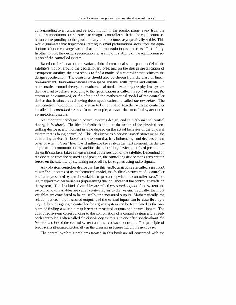
Any physical controller device that has thisfeedback structure is called afeedbackcontroller. In terms of its mathematical model, the feedback structure of a controlleris often represented by certain variables (representing what the controller ‘sees’) be-ing mapped to other variables (representing the influence that the controller exerts onthe system). The first kind of variables are calledmeasured outputs of the system, thesecond kind of variables are calledcontrol inputs to the system. Typically, the inputvariables are considered to becaused by the measured outputs. Mathematically, therelation between the measured outputs and the control inputs can be described by amap. Often, designing a controller for a given system can be formulated as the pro-blem of finding a suitable map between measured outputs and control inputs. Thecontrolled system corresponding to the combination of a control system and a feed-back controller is often calledthe closed-loop system, and one often speaks abouttheinterconnection of the control system and the feedback controller. The principle offeedback is illustrated pictorially in the diagram in Figure 1.1 on the next page.
The control synthesis problems treated in this book are all concerned with the
4 Introduction
�
�
��
��
Feedbackcontroller
System tobe controlled
measuredoutputs
controlinputs
......
......
Figure 1.1: The principle of feedback
design of feedback controllers: given a linear time-invariant state-space system, andcertain design specifications, find a feedback controller such that the design spec-ifications are fulfilled by the closed-loop system, or determine that such feedbackcontroller does not exist.
1.2 An example: instability of the geostationary orbit
In this example we will take a more detailed look at the system describing the motionof a communications satellite. The principle of such a satellite is that it serves as amirror for electromagnetic signals. In order not to be forced to continuously aim thetransmitters and receiving antennas at the satellite, it is desired that the satellite hasa fixed position with respect to these devices. This also has the advantage that thesatellite does not go down and rise, so that it can be used 24 hours a day.
In order to simplify the example, we will consider the motion of the satellite inthe equator plane. By taking the origin at the center of the earth, the position of thesatellite is given by its polar coordinates(r, θ). Introduce the following constants:
ME : = mass of the earth,
G : = earth’s gravitational constant,
� : = earth’s angular velocity,
MS : = mass of the satellite.
We assume that the satellite has on-board jets which make it possible to exert forcesFr (t) andFθ (t) to the satellite in the direction ofr andθ , respectively. Using New-ton’s law it can be verified that the equations of motion of the satellite are given by
r(t) = r(t)θ (t)2− G MEr(t)2
+ Fr (t)MS
,
θ (t) = −2 r(t)θ(t)r(t) + Fθ (t)
MSr(t) .
An example: instability of the geostationary orbit 5
The desired geostationary orbit is given by
θ(t) = θ0+�t,
r(t) = R0,
Fr (t) = 0,
Fθ (t) = 0,
whereR0 still has to be determined. We first check that this indeed yields a solution tothe equations of motion for suitableR0. By substitution in the differential equationswe obtain
0= R0�2− GME
R20
,
which yields
R0 = 3
√GME
�2 .
By taking the appropriate values for the physical constants in this formula, we findthat R0 is approximately equal to 42000 km. Thus the geostationary orbit is a circularorbit in the equator plane, at an altitude of approximately 35620 km over the equator(the radius of the earth being approximately 6380 km). It is convenient to replace theequations of motions by an equivalent system of four first order differential equationsby putting
x1 : = r(t)− R0,
x2 : = r(t),x3 : = θ(t)− (θ0+�t),x4 : = θ −�.
Note thatx3 is the deviation from the desired angle. This value can at any timeinstant be measured by an observer on the equator by comparing the actual positionof the satellite to the desired position. In terms of these new variables, the system isdescribed by
x1(t)x2(t)x3(t)x4(t)
=
x2(t)(x1(t)+ R0)(x4(t)+�)2− G ME
(x1(t)+R0)2 + Fr (t)
MS
x4(t)−2x2(t)(x4(t)+�)
x1(t)+R0+ Fθ (t)
MS(x1(t)+R0)
(1.1)
The equations (1.1) constitute a nonlinear state-space model with inputs and outputs.The control input isu = (Fr , Fθ )T, for the measured output one could takex 3. Thegeostationary orbit corresponds to the equilibrium solution given by
(x1, x2, x3, x4) = (0,0,0,0), Fr = 0, Fθ = 0.
6 Introduction
By Kepler’s law it is clear that if at timet0 the equilibrium solution is perturbed to,say,
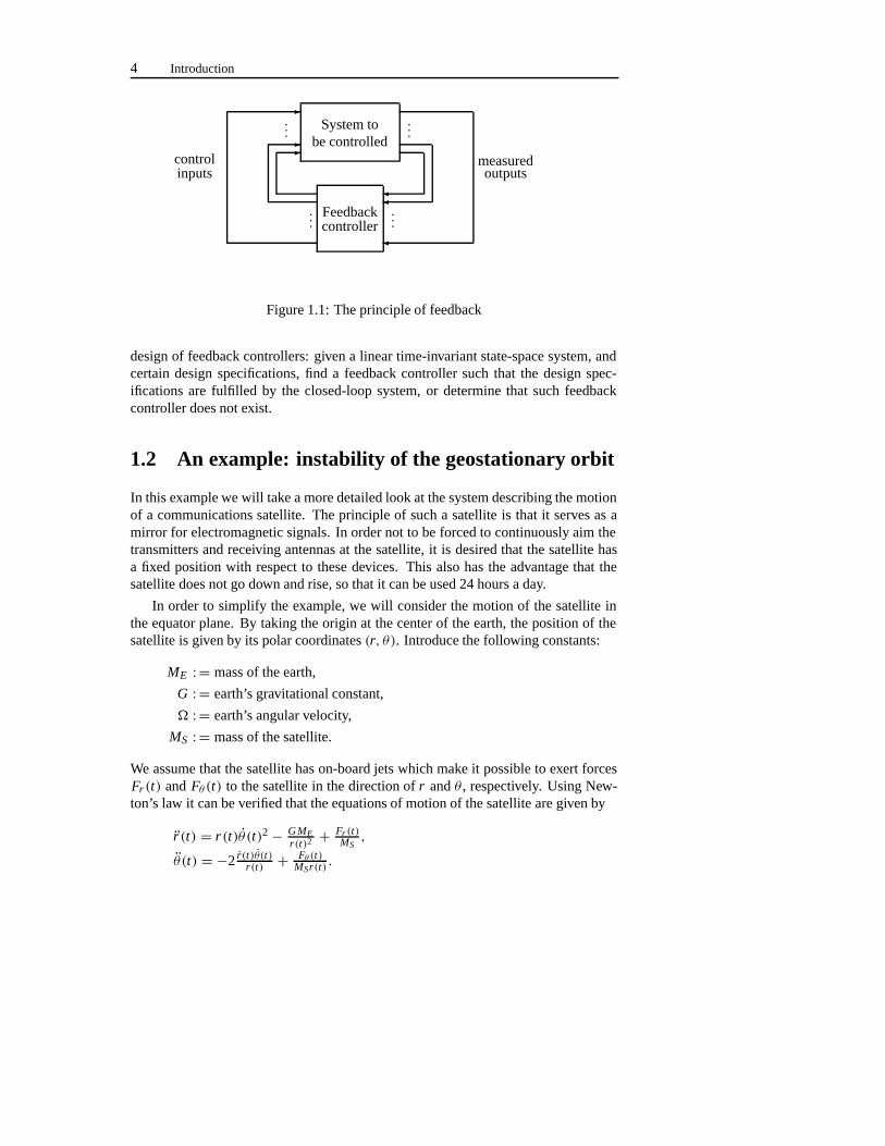
(x1(t0), x2(t0), x3(t0), x4(t0)) = (ξ1, ξ2, ξ3, ξ4),then the resulting orbit will be an ellipsoid in the equator plane with the earth in oneof its focuses. The angular velocity of the satellite with respect to the center of earthwill then no longer be constant, so to an observer on the equator the satellite willnot be in a fixed position, but will actually go down and rise periodically. Mathe-matically this can be expressed by saying that the equilibrium solution is not locallyasymptotically stable.What can we do about this? We still have the possibility toexert forces to the satellite in ther -direction and in theθ -direction. Also, the variablex3 can be measured. The control synthesis problem can now be formulated as: finda feedback controller that generates a control inputu = (Fr , Fθ )T on the basis of themeasured outputx3, in such a way that the equilibrium solution corresponding to thegeostationary orbit becomes locally asymptotically stable. Of course, it is not clear apriori whether such controller exists.
system
?
(FrFθ
)�
�x3
1.3 Linear control systems
The above is an example in which the system to be controlled is a nonlinear system.The vector(x1, x2, x3, x4)
T is called thestate variable of the system. Solutions to thedifferential equations (1.1) take their values in thestate space R4. The control inputu = (Fr , Fθ )T takes its values in theinput space R2, the measured outputx3 takes itsvalues in theoutput space R. More generally, a control system with state variablex ,state spaceRn , input variableu, input spaceRm , output variabley, and output spaceRp is given by the following equations:
x(t) = f (x(t), u(t)),y(t) = g(x(t), u(t)).
Here, f is a function fromRn × Rm to Rn andg is a function fromRn × Rm to Rp.If f andg are linear, then we obtain alinear control system. If f is linear then thereexist linear mapsA : Rn → Rn andB : Rm → Rn such thatf (x, u) = Ax + Bu. If
Example: linearization around the geostationary orbit 7
g is linear then there exist linear mapsC : Rn → Rp and D : Rm → Rp such thatg(x, u) = Cx + Du. The equations of the corresponding control system are then
x(t) = Ax(t)+ Bu(t),y(t) = Cx(t)+ Du(t).
This is called alinear, time-invariant, finite-dimensional state-space system. In thisbook we will exclusively deal with the latter kind of control system models. Manyreal life systems can be modeled very well by this kind of system models. Often, thebehavior of a nonlinear system can, at least in the neighborhood of an equilibriumsolution, be approximately modeled by such a linear system.
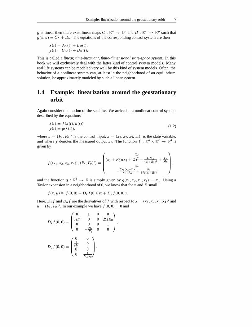
1.4 Example: linearization around the geostationaryorbit
Again consider the motion of the satellite. We arrived at a nonlinear control systemdescribed by the equations
x(t) = f (x(t), u(t)),y(t) = g(x(t)),
(1.2)
whereu = (Fr , Fθ )T is the control input,x = (x1, x2, x3, x4)T is the state variable,
and wherey denotes the measured outputx 3. The function f : R4 × R2 → R4 isgiven by
f ((x1, x2, x3, x4)T, (Fr , Fθ )
T) =
x2
(x1+ R0)(x4+�)2− G ME(x1+R0)
2 + FrMS
x4
−2x2(x4+�)x1+R0
+ FθMS(x1+R0)
,
and the functiong : R4 → R is simply given byg(x1, x2, x3, x4) = x3. Using aTaylor expansion in a neighborhood of 0, we know that forx andF small
f (x, u) ≈ f (0,0)+ Dx f (0,0)x + Du f (0,0)u.
Here,Dx f andDu f are the derivatives off with respect tox = (x1, x2, x3, x4)T and
u = (Fr , Fθ )T. In our example we havef (0,0) = 0 and
Dx f (0,0) =
0 1 0 03�2 0 0 2�R0
0 0 0 10 − 2�
R00 0
,
Du f (0,0) =
0 01
MS0
0 00 1
MS R0
.
8 Introduction
Here, we have used the fact thatG ME
R30= �2. Thus, for smallx = (x1, x2, x3, x4)
T
andu = (Fr , Fθ )T, the original nonlinear control system can be approximated by thelinear control system
x1(t) = x2(t),x2(t) = 3�2x1(t)+ 2�R0x4(t)+ Fr
MS,
x3(t) = x4(t),x4(t) = −2�
R0x2(t)+ Fθ
MS R0.
(1.3)
Of course this can be written as
x(t) = Ax(t)+ Bu(t),y(t) = Cx(t),
(1.4)
with A : = Dx f (0,0), B := Du f (0,0), andC : = (0 0 1 0). This linear control sys-tem is called thelinearization of the original system around the equilibrium solution(u, x, y) = (0,0,0).
1.5 Linear controllers
As explained, a feedback controller for a given control system is a mathematicalmodel that generates control input signals for the system to be controlled on the basisof measured outputs of this system. If we are dealing with a system in state spaceform given by the equations
x(t) = f (x(t), u(t)),y(t) = g(x(t), u(t)),
(1.5)
then a possible choice for the form of such a mathematical model is to mimic theform of the control system, and to consider pairs of equations of the form
w(t) = h(w(t), y(t)),u(t) = k(w(t), y(t)).
(1.6)
Any such pair of equations will be called a feedback controller for the system (1.5).The variablew is called the state variable of the controller, it takes its values inR �
for some�. The controller is completely determined by the integer�, together withthe functionsh andk. The measured outputy is taken as an input for the controller.On the basis ofy the controller determines the control inputu.
If we are dealing with a linear control system given by the equations
x(t) = Ax(t)+ Bu(t),y(t) = Cx(t)+ Du(t),
then it is reasonable to consider feedback controllers of a form that is compatiblewith the linearity of these equations. This means that we will consider controllers of
Example: regulation of the satellite’s position 9
the form (1.6) in which the functionsh andk are linear. Such controllers are alsorepresented by linear, time-invariant, finite-dimensional systems in state space form,given by
w(t) = Kw(t) + Ly(t),u(t) = Mw(t) + Ny(t),
(1.7)
whereK , L,M andN are linear maps. The state variable of the controller isw. Anypair of equations (1.7) is called alinear feedback controller .
1.6 Example: stabilizing the geostationary orbit
Our design specification is local asymptotic stability of the geostationary orbit. With-out going into the details, we mention the following important result on local asymp-totic stability of a given stationary solution of a system of first order nonlinear differ-ential equations:if the linearization around the stationary solution is asymptoticallystable, then the stationary solution itself is locally asymptotically stable. This meansthat if we succeed in finding a linear controller for the linearization (1.4), then thesame linear controller applied to the original nonlinear control system will make thegeostationary orbit locally asymptotically stable!
Consider the linearization (1.4) around this stationary solution. If we interconnectthis linear system with a linear controller of the form,
w(t) = Kw(t) + Ly(t),u(t) = Mw(t) + Ny(t),
(1.8)
then the resulting closed-loop system is obtained by substitutingu = Mw + Ny into(1.4) andy = Cx into (1.8). This yields(
x(t)w(t)
)=
(A + B NC B M
LC K
)(x(t)w(t)
). (1.9)
This system of first order linear differential equations is asymptotically stable if andonly if all eigenvaluesλ of the matrix
Ae : =(
A + B NC B MLC K
)
satisfy�e λ < 0, i.e., have negative real parts. A matrix with this property isreferred to as astability matrix. The problem is to find matricesK , L,M andN suchthat this property holds. Once we have found these matrices, the corresponding linearcontroller applied to the original nonlinear system will make the geostationary orbitlocally asymptotically stable. Indeed, the interconnection of (1.2) with (1.8) is givenby
x(t) = f (x(t),Mw(t) + Ng(x(t))),w(t) = Kw(t) + Lg(x(t)),
and its linearization around the stationary solution(0,0) is exactly given by (1.9).
10 Introduction
1.7 Example: regulation of the satellite’s position
In the previous section we discussed the problem of making the geostationary orbitasymptotically stable. This property guarantees that the statex = (x 1, x2, x3, x4)
T,after an initial perturbationx(0) = (ξ1, ξ2, ξ3, ξ4)
T away from the zero equilibrium,converges back to zero as time runs off to infinity. In the satellite example, we are verymuch interested in two particular variables, namelyx 1(t) = r(t) − R0 andx3(t) =θ(t)−(θ0+�t). The values of these variables express the deviation from the satellite’srequired position. It is very important that, after a possible initial perturbation awayfrom the zero solution, these values return to zero as quickly as possible. The designspecification of asymptotic stability alone is too weak to achieve this quick return tozero.
This motivates the following approach. Given the linear model (1.3) of the satel-lite’s motion around the geostationary equilibrium and a possible perturbationx(0) =ξ = (ξ1, ξ2, ξ3, ξ4)
T away from the equilibrium, express theperformance of the sys-tem by the following functional of the control inputu = (Fr , Fθ )T:
J (ξ, Fr , Fθ ) =∫ ∞
0αx2
1(t)+ βx22(t)+ γ F2
r (t)+ δF2θ (t)dt (1.10)
Here,α, β, γ , andδ are non-negative constants, calledweighting coefficients. Areasonable control synthesis problem is now to design a feedback controller that gen-erates input functionsu = (Fr , Fθ )T, for example on the basis of measurementsof the state variablesx = (x1, x2, x2, x4)
T, such that the performance functionalJ (ξ, Fr , Fθ ) is as small as possible, while at the same time the closed-loop system isasymptotically stable. More concretely, one could try to find a feedback controller ofthe form
u = Fx,
with F a linear map fromR4 to R2 that has to be determined, such that (1.10) isminimal, and such that the closed-loop system is asymptotically stable. Such feed-back controller whereu is a static linear function of the state variablex is called astatic state feedback control law. By a suitable choice of the weighting coefficients,it is expected that in the closed-loop system both
∫∞0 x2
1(t)dt and∫∞
0 x23(t)dt are
small, so thatx1(t) andx3(t) will return to a small neighborhood of zero quickly, asdesired. A feedback controller that minimizes the quadratic performance functional(1.10) is called alinear quadratic regulator. This terminology comes from the factthat the underlying control system is linear, and the performance functional dependsquadratically on the state and input variables.
1.8 Exogenous inputs and outputs to be controlled
Often, if we make a mathematical model of a real life physical system, we do not onlywant to specify the control inputs, but also a second kind of inputs, theexogenous
Example: including the moon’s gravitational field 11
inputs. These can be used, for example, to model unknown disturbances that act onthe system. Also, they can be used to ‘inject’ into the system the description of giventime functions that certain variables in the system are required to track. In this casethe exogenous inputs are calledreference signals. Often, apart from the measuredoutput, we want to include in our mathematical model a second kind of outputs, theoutputs to be controlled, also called theexogenous outputs. Typically, the outputs tobe controlled include those variables in the control system that we are particularlyinterested in, and that, for example, we want to keep close to certain, a priori given,values.
A general control system in state space form with exogenous inputs and outputsto be controlled is described by the following equations:
x(t) = f (x(t), u(t), d(t)),y(t) = g(x(t), u(t), d(t)),z(t) = h(x(t), u(t), d(t)).
(1.11)
Here,d represents the exogenous inputs. The functionsd are assumed to take theirvalues in some fixed finite-dimensional linear space, say,Rr . The variablez repre-sents the outputs to be controlled, which are assumed to take their values in, say,Rq . The variablesx , u andy are as before, and the functionsf, g andh are smoothfunctions mapping between the appropriately dimensioned linear spaces. Typically,the functionh is chosen in such a way thatz represents those variables in the systemthat we want to keep close to, or at, some prespecified valuez ∗, regardless of thedisturbance inputsd that happen to act on the system.
Again, if f , g andh are linear functions, then the equations take the followingform
x(t) = Ax(t) + Bu(t) + Ed(t),z(t) = C1x(t) + D11u(t) + D12d(t),y(t) = C2x(t) + D21u(t) + D22d(t),
for given linear mapsA, B, E,C1, D11, D12,C2, D21 andD22. These equations aresaid to constitute alinear control system in state space form with exogenous inputsand outputs. Many real life systems can be modelled quite satisfactorily in this way.Moreover, the behavior of nonlinear systems around equilibrium solutions is oftenmodelled by such linear systems.
1.9 Example: including the moon’s gravitational field
In the equations of motion of our satellite we did not include gravitational forcesacting on the satellite caused by other bodies than the earth. Now suppose that in oursatellite model we want to include the forces caused by the gravitational field of themoon. We can do this by including into our system the forces exerted by the moon onthe satellite as disturbance inputs, whose values are unknown. LetFM,r andFM,θ bethe forces applied by the moon in ther andθ direction, respectively. Including these
12 Introduction
into the model, we obtain
x1(t)x2(t)x3(t)x4(t)
=
x2(t)
(x1(t)+ R0)(x4(t)+�)2− G ME(x1(t)+R0)
2 + Fr (t)MS
+ FM,r (t)MS
x4(t)
−2x2(t)(x4(t)+�)x1(t)+R0
+ Fθ (t)MS(x1(t)+R0)
+ FM,θ (t)MS(x1(t)+R0)
(1.12)
We are particularly interested in the variablesx1(t) andx3(t), describing the deviationfrom the desired geostationary orbit(R0, θ0+�t). Thus, as output to be controlled wecan take the vector(x1, x3). In this way we exactly obtain a model of the form (1.11),with control inputu = (Fr , Fθ )T, exogenous inputd = (FM,r , FM,θ )
T, measuredoutputy = x3, and output to be controlledz = (x1, x3)
T.
Of course, an equilibrium solution is given by
(x1, x2, x3, x4) = (0,0,0,0),(Fr , Fθ ) = (0,0),(FM,r , FM,θ ) = (0,0).
By linearization around this stationary solution, we find that for small(x 1, x2, x3, x4),small (Fr , Fθ ) and small(FM,r , FM,θ ), our original control system is approximatedby
x1(t) = x2(t),
x2(t) = 3�2x1(t)+ 2�R0x4(t)+ Fr (t)MS
+ FM,r (t)MS
,
x3(t) = x4(t),
x4(t) = −2�R0
x2(t)+ Fθ (t)MS R0
+ FM,θ (t)MS R0
.y(t) = x3(t),
z(t) =(
x1(t)x3(t)
).
Of course, these equations constitute a linear control system in state space form withexogenous inputs and outputs:
x(t) = Ax(t)+ Bu(t)+ Ed(t),y(t) = C1x(t),z(t) = C2x(t),
(1.13)
with A andB as before,E : = B, C1 : =(0 0 1 0
)and
C2 : =(
1 0 0 00 0 1 0
).
If we interconnect this system with a linear controller of the form (1.8), then theclosed-loop system will be given by(
x(t)w(t)
)=
(A + B NC1 B M
LC1 K
)(x(t)w(t)
)+
(E0
)d(t),
z(t) = (C2 0
) (x(t)w(t)
).
(1.14)
Notes and references 13
Our control synthesis problem might now be to invent a linear controller such that,in the closed-loop system, the disturbance inputd (= (FM,r , FM,θ )) does not influ-ence the outputz. If a controller achieves this design specification, then it is saidto achievedisturbance decoupling. If this design specification is fulfilled, then, atleast according to the linear model, the satellite will remain in its geostationary or-bit once it has been put there, regardless of the gravitational forces of the moon. Ofcourse, part of the design problem would be to answer the question whether such con-troller actually exists. If it does not exist, one could weaken the design specification,and require that the influence of the disturbances on the outputs to be controlled beas small as possible, in some appropriate sense. One could, of course, also ask forcombinations of design specifications to be satisfied, for example both disturbancedecoupling and asymptotic stability of the closed-loop system, in the sense of section1.6. Alternatively, one could try to design a controller that makes the influence ofthe disturbances on the output to be controlled as small as possible, while making theclosed-loop system asymptotically stable, again in the sense of section 1.6.
1.10 Robust stabilization
In general, a mathematical model of a real life physical system is based on manyidealizing assumptions. Thus, in general, the control system that models a certain reallife phenomenon will not be a precise description of that phenomenon. Thus it mighthappen that a controller that asymptotically stabilizes the control system that we areworking with, does not make the real life system behave in a stable way at all, simplybecause the control system we are working with is not a good description of this reallife system. Sometimes, it is not unreasonable to assume that the correct descriptionrather liesin a neighborhood (in some appropriate sense) of the control system thatwe are working with (this control system is often calledthe nominal system). In orderto assure that a controller also stabilizes our real life system, we could formulatethe following design specification: given the nominal control system, together with afixed neighborhood of this system, find a controller that stabilizes all systems in thatneighborhood. If a controller achieves this design objective, we say that itrobustlystabilizes the nominal system.
As an example, consider the linear control system that models the motion of thesatellite around its stationary solution. This model was obtained under several ideal-izing assumptions. For example, we have neglected the dynamics of the satellite thatare caused by the fact that, in reality, it is not a point mass. If these additional dynam-ics were taken into account in the nonlinear control system, then we would obtain adifferent linearization, lying in a neighborhood (in an appropriate sense) of the orig-inal (nominal) linearization, described in section 1.4. One could then try to design arobustly stabilizing controller for the nominal linearization. Such controller will notonly stabilize the nominal control system, but also all systems in a neighborhood ofthe nominal one.

14 Introduction
1.11 Notes and references
Many textbooks on control systems design, and the mathematical theory of systemsand control are available. Among the more recent engineering oriented textbookswe mention the books by Van de Vegte [202], Phillips and Harbor [145], Franklin,Power and Emami-Naeini [49], and Kuo [101]. Among the textbooks that concentratemore on the mathematical aspects of systems and control we mention the classicaltextbooks by Kwakernaak and Sivan [105] and Brockett [25]. The satellite examplethat was discussed in this chapter is a standard example in several textbooks; see forinstance the book by Brockett [25]. We also mention the seminal book by Wonham[223], which was the main source of inspiration for the geometric ideas and methodsused in this book. Other relevant textbooks are the books by Kailath [90], Sontag[181], Maciejowski [118], and Doyle, Francis and Tannenbaum, [40]. As more morerecent textbooks on control theory for linear systems we mention the books by Greenand Limebeer [66], Zhou, Doyle and Glover [232], and Dullerud and Paganini [42].For textbooks on system identification and modelling we would like to refer to thebooks by Ljung [112] and Ljung and Glad [113]. For textbooks on systems andcontrol theory for nonlinear systems, we refer to the books by Isidori [86], Nijmeijerand Van der Schaft [134], Khalil [99], and Vidyasagar [208].
Chapter 2
Mathematical preliminaries
In this chapter we start from the assumption that the reader is familiar with the conceptof vector spaces (or linear spaces) and with linear maps. The objective of this chapteris to give a short summary of the standard linear-algebra tools to be used in this bookwith special emphasis on the geometric (as opposed to matrix) properties.
2.1 Linear spaces and subspaces
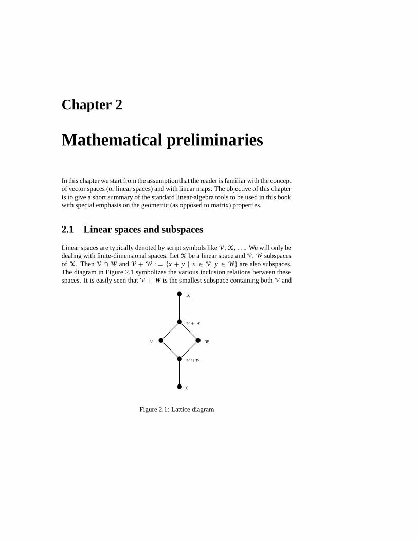
Linear spaces are typically denoted by script symbols likeV,X, . . .. We will only bedealing with finite-dimensional spaces. LetX be a linear space andV,W subspacesof X. ThenV ∩W andV +W : = {x + y | x ∈ V, y ∈ W} are also subspaces.The diagram in Figure 2.1 symbolizes the various inclusion relations between thesespaces. It is easily seen thatV +W is the smallest subspace containing bothV and
0
V ∩W
V +W
W
X
V
Figure 2.1: Lattice diagram
16 Mathematical preliminaries
W , i.e., if a subspaceL satisfiesV ⊂ L andW ⊂ L thenV +W ⊂ L. Similarly,V∩W is the largest subspace contained in bothV andW . The fact that for every pairof subspaces there exists a smallest subspace containing both subspaces and a largestsubspace contained in both spaces, is expressed by saying that the set of subspaces ofX forms alattice, and diagram in Figure 2.1 is called alattice diagram.
If V,W andR are subspaces andV ⊂ R then
R ∩ (V +W) = V + (R ∩W). (2.1)
This formula, which can be proved by direct verification (see exercise 2.1), is calledthemodular rule. Let V1,V2, . . . ,Vk be subspaces. Then they are called(linearly)independent if every x ∈ V1 + V2 + · · · + Vk has aunique representation of theform x = x1 + x2 + · · · + xk with xi ∈ Vi (i = 1, . . . , k), equivalently, ifxi ∈Vi (i = 1, . . . , k) andx1 + · · · + xk = 0 imply x1 = · · · = xk = 0. Still anothercharacterization is
Vi ∩∑j =i
V j = 0 (i = 1, . . . , k). (2.2)
Here, the symbol 0 is used to denote the null subspace of a vector space, i.e. thesubspace consisting only of the element 0. IfV1, . . . ,Vk are independent subspaces,their sumV is called thedirect sum of V1, . . . ,Vk and it is written
V = V1⊕ · · · ⊕Vk =k⊕
i=1
Vk .
If V is a subspace then there exists a subspaceW such thatV ⊕W = X. Such asubspace is called a(linear) complement of V. It can be constructed by first choosinga basisq1, . . . , qk of V and then extending it to a basisq1, . . . , qn of X. Then thespan ofqk+1, . . . , qn is a complement ofV, as can easily be verified. Obviously, acomplement is not unique.
The linear spaces we are interested in are spaces over the fieldR of real num-bers. For some purposes, however, it is convenient to allow also complex vectors andcoefficients. We denote byC the field of complex numbers. We use the complexextensionXC of a given linear spaceX, consisting of all vectors of the formv+ iw,wherev andw are inX. Many statements made in terms ofXC can easily be trans-lated to corresponding results aboutX. In this book, we will freely use the complexextension, often without explicitly mentioning it.
2.2 Linear maps
For a linear mapA : X→ Y, we define
ker A : = {x ∈ X | Ax = 0},im A : = {Ax | x ∈ X}, (2.3)
Linear maps 17
called thekernel andimage of A, respectively. These are linear spaces. We say thatA is surjective if im A = Y andinjective if ker A = 0. Also, A is calledbijective (oran isomorphism) if A is injective and surjective. In this case,A has an inverse map,usually denoted byA−1. It is also known that a bijectionA : X → Y exists if andonly if dim X = dimY (supposing, as we always do, that the linear spaces are finitedimensional).
In general, ifA : X→ Y is a, not necessarily invertible, linear map and ifV is asubspace ofY, then theinverse image of V is the subspace ofX defined by
A−1V : = {x ∈ X | Ax ∈ V}
Given A : X → X and a subspaceV of X, we say thatV is A-invariant (or,if the mapA is supposed to be obvious, simplyinvariant) if for all x ∈ V we haveAx ∈ V, which can be written asAV ⊂ V. The concept of invariance will play acrucial role in this book.
One can consider various types of restriction of a linear map:
• If B : U → X is a linear map satisfying imB ⊂ V whereV is a subspaceof X then thecodomain restriction of B is the mapB : U → V satisfyingBu : = Bu for all u ∈ U. We will not use a special notation for this type ofrestriction.
• If C : X → Y andV ⊂ X then the mapC : V → Y defined byCx : = Cxfor x ∈ V, is called the(domain) restriction of C to V, and it is denotedC | V.
• If A : X → X andV ⊂ X is anA-invariant subspace then the mapA : V →V defined byAx : = Ax for x ∈ V is called therestriction of A to V, notationA | V.
These somewhat abstract definitions will be clarified later on in terms of matrixrepresentations. IfX is ann-dimensional space andq1, . . . , qn is a basis then everyvectorx ∈ X has a unique representation of the form
x = x1q1+ · · · + xnqn.
The coefficients of this representation, written as a column vector inR n , form thecolumn of x with respect to q1, . . . , qn:
x =
x1...
xn
.
For typographical reasons, we often write this column as(x 1, . . . , xn)T, where the ‘T’
denotes transposition. Ifq1, . . . , qn is a basis ofX andr1, . . . , rp is a basis ofY andC : X→ Y is a linear map, thematrix of C with respect to the basesq1, . . . , qn and
18 Mathematical preliminaries
r1, . . . , rp is formed by writing next to each other the columns ofCq 1, . . . ,Cqn withrespect to the basisr1, . . . , rp. The result will look like
(C) : =
c11 · · · c1n...
...
cp1 · · · cpn
,
where(c1i , . . . , cpi )T is the column ofCqi with respect tor1, . . . , rp . We use brack-
ets aroundC here to emphasize that we are talking about the matrix of the map. Wewill use the notationR p×n for the set ofp × n matrices. Hence(C) ∈ R p×n . Oncethe bases are fixed, the mapC and its matrix determine each other uniquely. Also, theoperations of matrix addition, scalar multiplication, product of matrices correspond toaddition of maps, scalar multiplication of a map, composition of maps, respectively.For this reason it is customary to identify maps with matrices, once the bases of thegiven spaces are given and fixed. The advantage of the matrix formulation over themore abstract linear-map formulation is that it allows for much more explicit calcula-tions. On the other hand, if one works with linear maps, one does not have to specifybases, which sometimes makes the treatment much more elegant and transparent.
If V ⊂ X then a basisq1, . . . , qn of X for whichq1, . . . , qk is a basis ofV (wherek = dimV) is called a basis ofX adapted to V. More generally, ifV1,V2, . . . ,Vr
is a chain of subspaces (i.e.,V1 ⊂ V2 ⊂ · · · ⊂ Vr ), then a basisq1, . . . , qn of X issaid to beadapted to this chain if there exist numbersk 1, . . . , kr such thatq1, . . . , qki
is a basis ofVi for i = 1, . . . , r . Finally, if V1, . . . ,Vr are subspaces ofX such thatX = V1⊕V2⊕ · · · ⊕Vr , we say that a basisq1, . . . , qn is adapted to V1, . . . ,Vr ifthere exist numbersk1, . . . , kr+1 such thatk1 = 1, kr+1 = n+1 andqki , . . . , qki+1−1is a basis ofVi for i = 1, . . . , r .
We illustrate the use of matrix representations for the restriction operations intro-duced earlier in this section.
• If B : U → X is a linear map satisfying imB ⊂ V, we choose a basisq1, . . . , qn of X adapted toV. Let p1, . . . , pm be a basis ofU. Then thematrix representation ofB with respect to the chosen bases is of the form
(B) =(
B10
), (2.4)
whereB1 ∈ Rk×m (k : = dimV). This particular form is a consequence of thecondition imB ⊂ V. The matrix of the codomain restrictionB : U→ V withrespect to the basesp1, . . . , pm andq1, . . . , qk is B1.
• Let C : X → Y andV ⊂ X. Let q1, . . . , qn be a basis ofX adapted toV.Furthermore, letr1, . . . , rp be a basis ofY. The matrix ofC with respect toq1, . . . , qn andr1, . . . , rp is (C) = (C1 C2), whereC1 ∈ Rp×k andC2 ∈Rp×(n−k). The matrix ofC | V with respect to these bases isC1.
• Let A : X → X,V ⊂ X such thatAV ⊂ V. Let q1, . . . , qn be a basis ofX
Inner product spaces 19
adapted toV. The matrix ofA with respect to this basis is
(A) =(
A11 A120 A22
). (2.5)
The propertyA21 = 0 is a consequence of theA-invariance ofV. The matrixof A | V is A11.
2.3 Inner product spaces
We assume that the reader is familiar with the concept of inner product. A linearspace over the fieldR with a real inner product is called areal inner product space. Alinear space over the fieldC with a complex inner product is called acomplex innerproduct space. The most commonly used real inner product space is the linear spaceRn with the inner product(x, y) : = x T y. The most commonly used complex innerproduct space is the linear spaceCn with the inner product(x, y) : = x ∗y (here, ‘∗’denotes the conjugate transposition, i.e.x ∗ = x T).
If X is a (real or complex) inner product space and ifV is a subspace ofX, thenV⊥ will denote the orthogonal complement ofV. It is easy to see that for any pair ofsubspacesV, W of X the following equality holds:
(V ∩W)⊥ = V⊥ +W⊥
Let X andY be (real or complex) inner product spaces with inner products( , )X
and( , )Y, respectively. IfC : X→ Y is a map, then theadjoint C ∗ : Y → X ofC is the map defined by
(x,C∗y)X = (Cx, y)Y (2.6)
for all x in X andy in Y. It can easily be seen that there exists a unique map satisfyingthese properties. IfX is a (real or complex) inner product space and ifA : X → Xis a map, then it can be shown by direct verification that the following holds:
(A−1V)⊥ = A∗V⊥.
It is also easy to verify that ifV is A-invariant, thenV⊥ is A∗-invariant.
If X andY are real inner product spaces, ifq1, . . . , qn andr1, . . . , rp are or-thonormal bases ofX andY, respectively, and if(C) is the matrix ofC with respectto these bases, then the matrix of the adjoint mapC ∗ is equal to the transposed(C)T
of (C). Indeed, ifx andy denote the columns ofx andy, respectively, with respectto the given bases, then (2.6) is equivalent to
xT(C∗)y = x T(C)T y
for all x in Rn andy in Rp.
In the same way, one can show that ifX andY arecomplex inner product spaces,if q1, . . . , qn andr1, . . . , rp are orthonormal bases ofX andY, respectively and if
20 Mathematical preliminaries
(C) is the matrix ofC with respect to these bases, then the matrix of the adjoint mapC∗ is equal to the conjugate transposed(C)∗ of (C).
As noted in section 2.2, once the bases are fixed, we will identify maps withmatrices. In this book we will usually work with the real inner product spaceR n withinner product(x, y) : = x T y. Therefore, instead of using the terminology ‘adjoint’of a map and using the notationC ∗, we will in this book often use the terminology’transposed’ and use the notationC T.
2.4 Quotient spaces
A linear subspaceV gives rise to the equivalence relation:
x ∼ y :⇐⇒ x − y ∈ V.
on X. The set of equivalence classes is called thequotient space or factor space ofX moduloV, and it is denotedX/V. For anyx ∈ X, the equivalence class of whichx is an element is often denoted byx . There is a natural mapping : X → X/V,called thecanonical projection of X ontoX/V and defined byx : = x . The setX/V =: X is made into a linear space by
x + y : = x + y, λx : = λx .
It can be shown that addition and scalar multiplication are well defined by these for-mulas.
Also, these formulas state that is a linear map. Obviously, is surjective andker = V. The following result is of importance:
dimV + dimX/V = dimX.
In fact, letq1, . . . , qn be a basis ofX adapted toV and let dimV = k. Thenq1 =· · · = qk = 0, where the bar denotes the projection. Hence, ifx is an arbitraryelement ofX/V andx is a representative, we writex = λ1q1 + · · · + λnqn. Takingthe image inX/V, we get
x = λ1q1+ · · · + λnqn = λk+1qk+1 + · · · + λnqn.
It follows that every element ofX/V can be written as a linear combination ofqk+1, . . . , qn. On the other handqk+1, . . . , qn are independent. In fact, ifλk+1qk+1+· · · + λnqn = 0, thenq : = λk+1qk+1 + · · · + λnqn ∈ V, henceq can be written as alinear combination ofq1, . . . , qk . The result is
λk+1qk+1+ · · · + λnqn = λ1q1+ · · · + λkqk .
Now it follows from the independence ofq1, . . . , qn thatλk+1 = · · · = λn = 0.
Let A : X→ X, letV denote anA-invariant subspace and letX : =X/V. Thenwe define thequotient map A : X → X by Ax : = Ax . It is easily verified that
Eigenvalues 21
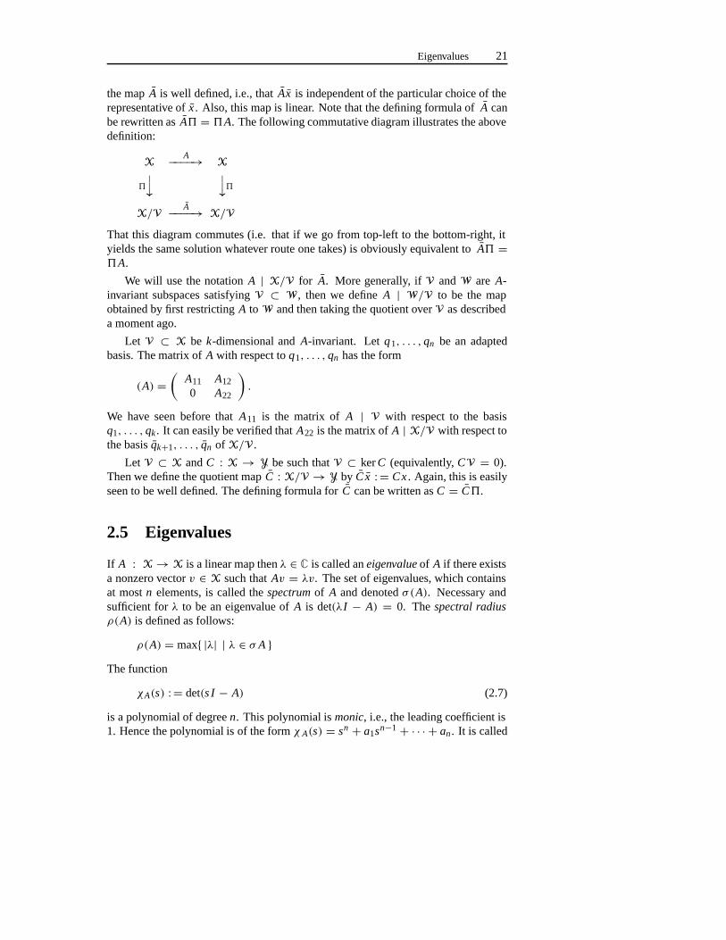
the mapA is well defined, i.e., thatAx is independent of the particular choice of therepresentative ofx . Also, this map is linear. Note that the defining formula ofA canbe rewritten asA = A. The following commutative diagram illustrates the abovedefinition:
XA−−−−→ X
� �X/V
A−−−−→ X/V
That this diagram commutes (i.e. that if we go from top-left to the bottom-right, ityields the same solution whatever route one takes) is obviously equivalent toA =A.
We will use the notationA | X/V for A. More generally, ifV andW are A-invariant subspaces satisfyingV ⊂ W , then we defineA | W/V to be the mapobtained by first restrictingA to W and then taking the quotient overV as describeda moment ago.
Let V ⊂ X be k-dimensional andA-invariant. Letq1, . . . , qn be an adaptedbasis. The matrix ofA with respect toq1, . . . , qn has the form
(A) =(
A11 A120 A22
).
We have seen before thatA11 is the matrix of A | V with respect to the basisq1, . . . , qk . It can easily be verified thatA22 is the matrix ofA | X/V with respect tothe basisqk+1, . . . , qn of X/V.
Let V ⊂ X andC : X → Y be such thatV ⊂ kerC (equivalently,CV = 0).Then we define the quotient mapC : X/V → Y by C x : = Cx . Again, this is easilyseen to be well defined. The defining formula forC can be written asC = C.
2.5 Eigenvalues
If A : X→ X is a linear map thenλ ∈ C is called aneigenvalue of A if there existsa nonzero vectorv ∈ X such thatAv = λv. The set of eigenvalues, which containsat mostn elements, is called thespectrum of A and denotedσ(A). Necessary andsufficient forλ to be an eigenvalue ofA is det(λI − A) = 0. Thespectral radiusρ(A) is defined as follows:
ρ(A) = max{ |λ| | λ ∈ σ A }The function
χA(s) : = det(s I − A) (2.7)
is a polynomial of degreen. This polynomial ismonic, i.e., the leading coefficient is1. Hence the polynomial is of the formχ A(s) = sn + a1sn−1 + · · · + an. It is called
22 Mathematical preliminaries
thecharacteristic polynomial of A. Its zeros are exactly the eigenvalues ofA. Anynonzero vectorv such thatAv = λv is called aneigenvector of A corresponding tothe eigenvalueλ. The set of eigenvectors corresponding toλ is a linear space equalto ker(λI − A) with the zero element removed.
Let V be anA-invariant subspace and letB : = A | V (the restriction, see section2.2). Then, obviously, every eigenvalue ofB is an eigenvalue ofA. We can make astronger statement:χB is a divisor ofχA. In order to see this, we choose a basis ofX adapted toV, and we obtain the matrix representation
(A) =(
A11 A120 A22
). (2.8)
HenceχA(s) = det(s I − (A)) = det(s I − A11)det(s I − A22). On the other hand,A11 is the matrix ofB with respect to the chosen basis. Hence
det(s I − A11) = χB(s),
which proves the statement. We also see that the quotient mapA : X/V → X/Vhas a divisor ofχA as characteristic polynomial, becauseA22 is the matrix ofA withrespect to a suitable basis (see section 2.4).
From section 2.3, recall that ifX is an inner product space and ifV is A-invariant,then V⊥ is AT-invariant. LetC : = AT | V⊥. We claim that the characteristicpolynomialχ A of the quotient mapA is equal to the characteristic polynomialχC
of the restricted mapC . To see this, choose an orthonormal basis ofX adapted toV,V⊥ to obtain the matrix representation (2.8). Obviously,
(A)T =(
AT
11 0AT
12 AT
22
)
is a matrix representation of the adjoint mapA T. Thus,A22 is a matrix representationof A, while AT
22 is a matrix representation ofC . Hence,
χ A = det(s I − A22) = det(s I − AT
22) = χC .
In particular, we have now proven the following useful formula:
σ(A | X/V) = σ(AT | V⊥). (2.9)
Let A : X→ X and letp(s) = a0sm + a1sm−1+ · · · + am be a polynomial. Wedefinep(A) : = a0Am + a1Am−1 + · · · + am I . This substitution has the followingproperties (herep andq are polynomials):
p(A)q(A) = (pq)(A), p(A)+ q(A) = (p + q)(A). (2.10)
In particular,p(A) andq(A) commute. Furthermore, we have thespectral mappingtheorem (see exercise 2.3):
σ(p(A)) = {p(λ) | λ ∈ σ(A)}, (2.11)
Eigenvalues 23
which is sometimes abbreviated toσ(p(A)) = p(σ (A)). Another very famous andimportant result is theCayley-Hamilton theorem:
χA(A) = 0. (2.12)
Theorem 2.1 Let A : X→ X and suppose that χ A is factorized as χA = pq, wherep and q are monic coprime polynomials. Define V : = ker p(A) and W : = kerq(A).Then we have
(i) V = im q(A),W = im p(A),
(ii) V ⊕W = X,
(iii) V and W are A-invariant,
(iv) χA|V = p, χA|W = q.
We say that two polynomials arecoprime (or relatively prime) if they do not havea common factor, or equivalently, a common (complex) zero. An equivalent conditionis: there exist polynomialsr ands such thatr p + sq = 1. Furthermore,p | q meansthat p is a divisor ofq.
Proof of theorem 2.1 : Let r ands be such thatr p + sq = 1. SubstitutingA intothis equation, we find thatI = r(A)p(A)+ s(A)q(A) (see (2.10)). Hence, for everyx ∈ X, the following equations hold:
x = r(A)p(A)x + s(A)q(A)x = p(A)r(A)x + q(A)s(A)x . (2.13)
(i) Note that ifx ∈ im q(A) thenx = q(A)y for somey. Hence
p(A)x = χA(A)y = 0,
so thatx ∈ V. Conversely, ifx ∈ V then p(A)x = 0 and hence, by (2.13),x =s(A)q(A)x = q(A)s(A)x ∈ im q(A). The proof ofW = im p(A) is similar.
(ii) If x ∈ V ∩W then p(A)x = 0 andq(A)x = 0. Hence, by (2.13),x = 0.That is,V andW are independent. It also follows from (2.13) that everyx ∈ X is anelement of imp(A)+ im q(A) = W + V.
(iii) If p(A)x = 0 thenp(A)Ax = Ap(A)x = 0.
(iv) We use lemma 2.2 which is stated directly after the current proof. Now letα : = χA|V . Thenα andq are coprime. In fact, ifα(λ) = 0 there existsx ∈ V, x = 0such thatAx = λx . Then p(A)x = p(λ)x = 0 and hencep(λ) = 0. It follows thatq(λ) = 0 (sincep andq are coprime). Asα | χ A, q | χA andα andq are coprime,the lemma implies thatαq | χA. As a consequence,α | p. Similarly, we have thatβ : = χA|W dividesq. Since deg(αβ) = deg(pq) = n, we must haveα = p andβ = q. This completes the proof of theorem 2.1
24 Mathematical preliminaries
Lemma 2.2 If p, q and r are polynomials satisfying p | r and q | r , and p and q arecoprime then pq | r .
Proof : Let u andv be such thatup + vq = 1. Thenpq | vqr and pq | upr andhencepq | r sincer = upr + vqr .
Note that the matrix ofA with respect to a basisq1, . . . , qn adapted toV,W is ofthe form(
A11 00 A22
).
whereχA11 = p andχA22 = q.
2.6 Differential equations
In this section, we consider the linear homogeneous time-invariant differential equa-tion
x(t) = Ax(t), (2.14)
whereA : X → X is a linear map andX an n-dimensional space. The equationis calledlinear because the right-hand side is a linear function ofx(t). It is calledhomogeneous because the right-hand side is zero forx(t) = 0. (An equation of theform x = Ax(t) + f (t) with f (t) = 0 is calledinhomogeneous). The equation iscalledtime invariant becauseA is independent oft . (One also says that the equationhasconstant coefficients). If A would be allowed to be time dependent, the equationwould be calledtime varying.
In order to specify the solution of (2.14), one has to provide an initial value. Thesolution of theinitial value problem: find a functionx satisfying
x = Ax, x(0) = x0, (2.15)
is denoted byx(t, x0). In the scalar case(n = 1, A = a), it is well known thatx(t, x0) = eat x0.
In order to have a similar result for the multivariable case, we introduce the matrixexponential function
eAt : = exp(At) : =∞∑
k=0
tk Ak
k! . (2.16)
Since‖Ak‖ � ‖A‖k for all k, the sum is dominated by∑(|t|‖A‖)k/k!. This series
converges for everyt and hence so does the series (2.16). Also, (2.16) is a powerseries, so that term by term differentiation is allowed. Hence,d
dt eAt = AeAt = eAt A.It follows thatx(t, x0) = eAt x0.
The concept of invariant subspace has an important significance for systems ofdifferential equations:
Differential equations 25
Definition 2.3 A subspace V is called an invariant subspaceof (2.15) if every solu-tion of (2.15) that starts in V, remains in V for all t � 0. More explicitly, if for everyx0 ∈ V, we have that x(t, x0) ∈ V for all t > 0.
Theorem 2.4 A subspace V is an invariant subspace of (2.15) if and only if V isA-invariant.
Proof : If x0 ∈ V, thenAx0 ∈ V, A2x0 ∈ V, and, by induction,Akx0 ∈ V for all k.It follows that for allm, the vector
m∑k=0
tk Ak
k! x0 ∈ V.
SinceV is a subspace of the finite dimensional linear spaceX, it is closed in theEuclidean topology. Thus we infer thate At x0 ∈ V.
Conversely, ifx(t, x0) ∈ V for all t > 0 and allx0 ∈ V, then
Ax0 = limt↓0
t−1(et A − I )x0 = limt↓0
t−1(x(t, x0)− x0) ∈ V,
again becauseV is closed.
The definition ofe At is not very suitable for the investigation of the behavior ofx(t) for large values oft . This behavior is more adequately given by the spectrumof A. We will not give a complete picture of the behavior in the most general case,because it is rather complicated and also not necessary. A convenient formula for theexponential function is given by Cauchy’s integral in the complex plane:
eAt = 1
2π i
∫C
ezt (z I − A)−1 dz, (2.17)
where the contour of integrationC encloses all eigenvalues ofA. This formula canbe proven by using the Neumann expansion
(z I − A)−1 = z−1I + z−2A + z−3A2+ · · ·for |z| � ‖A‖. Because this is a power series, we can perform integration term wise.Hence:
1
2π i
∫C
ezt(z I − A)−1 dz =∞∑
k=0
fk(t),
where
fk(t) : = 1
2π i
∫C
ezt z−k−1 dz Ak = tk Ak
k! .
26 Mathematical preliminaries
It follows from Cramer’s rule that(z I − A)−1 is of the form
B(z)/ det(z I − A),
whereB(z) is a matrix of which the entries are polynomials ofz. Hence, each entry of(z I − A)−1 is a rational function and the poles of this function are eigenvalues ofA.If we perform partial-fraction decomposition, we find that the entries of(z I − A)−1
can be written as a linear combination of functions of the form(z − λ)−k . As aconsequence,e At is a linear combination of functions of the form
1
2π i
∫C
ezt(z − λ)−k dz = tk−1eλt
k! ,
where theλ’s are eigenvalues ofA.
Definition 2.5 A function that is a linear combination of functions of the form t keλt ,where the k’s are nonnegative integers and λ ∈ C, is called a Bohl function. Thenumbers λ that appear in this linear combination (and cannot be canceled) are calledthe characteristic exponentsof the Bohl function. The set of characteristic exponentsof a Bohl function p is called the spectrumof the function and denoted σ(p).
The previous discussion implies:
Theorem 2.6 The entries of e At are Bohl functions. Their characteristic exponentsare eigenvalues of A. Each eigenvalue of A appears as a characteristic exponent ofsome entry of e At .
The last statement of the theorem follows from the fact that for everyλ ∈ σ(A)with corresponding eigenvectorv, the functionx(t) : = e λtv is a solution of (2.14)and hence equal tox(t, v). On the other hand, according to (2.16) we havex(t, v) =eAtv. Hence there must be at least one entry ofe At with exponentλ. Note that, ifone insists on having real functions and vectors, one has to define Bohl functions aslinear combinations of the functions of the formt keαt cosωt andt keαt sinωt , wherek is an integer andα andω are real numbers.
The following result is easily verified:
Theorem 2.7 If p and q are Bohl functions then p + q, pq and p are also Bohlfunctions. Furthermore, σ(pq) ⊂ σ(p) + σ(q), σ (p + q) ⊂ σ(p) ∪ σ(q) andσ( p) ⊂ σ(p). Also, if r(t) : = ∫ t
0 p(τ ) dτ then r is a Bohl function with σ(r) ⊂σ(p) ∪ {0}.
The concept of Bohl function can be extended to vector-valued and matrix-valuedfunctions in the obvious way. Every vector or matrix whose entries are Bohl functionswill also be called a Bohl function.
Next we consider the inhomogeneous initial value problem
x = Ax + f (t), x(0) = x0. (2.18)
Stability 27
The solution to this problem can also be expressed in terms of the matrix exponentialfunction. For this, we introduce the functionz(t) : = e−At x(t). We note that thisfunction satisfies
z(t) = −Az(t)+ e−At (Ax(t)+ f (t)) = e−At f (t),
a differential equation which can be solved by quadrature. The solution is
z(t) = z(0)+∫ t
0e−Aτ f (τ ) dτ.
Sincex(t) = eAt z(t), it follows that
x(t) = eAt x0+∫ t
0eA(t−τ ) f (τ ) dτ, (2.19)
where we have used thatz(0) = x0. Formula (2.19) is called thevariations of con-stants formula. It is valid for any continuous functionf . If f is an arbitrary integrablefunction, the expression in the right-hand size of (2.19) is still defined. We will viewthe function defined by the right-hand side of (2.19) as the solution of (2.18) in ageneralized sense. As a corollary of theorem 2.7 and this formula we have
Theorem 2.8 If f (t) is a Bohl function then the solution of (2.18) is also a Bohlfunction.
2.7 Stability
The concept of stability plays an important role in the theory of differential equations.In the general theory, where time varying and nonlinear systems are considered, thedefinitions are rather involved and the distinctions are subtle. For the very simplesituation we are considering here, a drastic simplification of the treatment is possible.In particular, we will not need the concept that is called (Liapunov) stability, althoughin section 3.8 we will briefly introduce the Liapunov equation and its relation tostability will be presented.
What is important in control theory is a concept that is usually calledasymptoticstability in the theory of ordinary differential equations. We will refer to this conceptas stability, omitting the adjective ‘asymptotic’. For linear time-invariant systems,this concept can be defined very simply:
Definition 2.9 The system x = Ax is called stableif every solution tends to zero fort →∞.
A condition for stability can be derived from the following result
Theorem 2.10 Let p be a Bohl function and let the spectral abscisof p be defined by
�(p) : = max{ �eλ | λ ∈ σ(p) }. (2.20)
Then the following statements hold:
28 Mathematical preliminaries
(i) If �(p) < 0 or, equivalently, every exponent λ of p satisfies �eλ < 0 thenp(t) → 0 (t → ∞). More specifically, for every γ > 0 there exists M > 0such that for all t � 0 we have |p(t)| � Me−γ t .
(ii) For all α > �(p) there exists M > 0 such that for all t � 0 we have |p(t)| �Meαt .
Proof : (i) It is well known thatt keλt → 0 (t → ∞) if �eλ < 0. Hence a Bohlfunction converges to zero if all its exponents have a negative real part. In particular,such a function is bounded. Forγ , take any positive real number such that�(p) <−γ < 0. Then the functionq(t) = eγ t p(t) still is a Bohl function satisfying that�(q) < 0. There existsM > 0 such that|q(t)| � M , which implies that|p(t)| �Me−γ t .
(ii) If p is a Bohl function andβ = �(p) then for everyα > β, the functionq(t) = e−αt p(t) is a Bohl function satisfying�(q) < 0. Henceq is bounded andthere exists a numberM such that|p(t)| � Meαt .
We use the notation
�(A) : = max{�eλ | λ ∈ σ(A)} (2.21)
for thespectral abscis of a linear map. Then we have
Corollary 2.11 System (2.14) is stable if and only if �(A) < 0. In this case, thereexist positive numbers M and γ such that the inequality ‖e At‖ � Me−γ t holds forall t > 0.
Proof : In view of the above, we only need to prove necessity. Suppose�(A) � 0and letλ ∈ σ(A), Av = λv, v = 0 and�eλ � 0. Theneλtv is a solution of (2.14)that does not tend to zero.
For some purposes, it is desirable to have different notions of stability. For in-stance, one might be interested in having a special rate of convergence, i.e., one mightwant the solutions to satisfy conditions likeeαt x(t)→ 0 (t →∞), for a prescribedα. Or, one wants to avoid high frequencies in the functions, i.e., one imposes on theexponents a condition like| �mλ| � β for a prescribedβ. For discrete-time systems,one can prove that the stability condition is|λ| < 1 for all eigenvalues. These ex-amples suggest a generalization of the stability condition giving rise to conditions onthe eigenvalues and exponents of the formλ ∈ C g , whereCg is a prescribed part of thecomplex plane, thought of as the ‘good’ part. The complement ofC g is often denotedCb. For the original stability condition, we haveCg = C− := {λ ∈ C | �eλ < 0}.Similarly we will use:
C0 : = {λ ∈ C | �eλ = 0}C+ := {λ ∈ C | �eλ > 0}
Stability 29
We introduce a term forCg :
Definition 2.12 A subset Cg of C is called a stability domainif Cg ∩ R is nonemptyand Cg is symmetric with respect to the real axis (i.e., λ ∈ Cg =⇒ λ ∈ Cg). If Cg isa stability domain, a Bohl function p is called Cg-stableif σ(p) ⊂ Cg. The systemx = Ax is called Cg-stableif every solution is a Cg-stable Bohl function. Finally, alinear map A is called Cg-stableif σ(A) ⊂ Cg. A linear map is called Cg-antistableif σ(A) ∩ Cg is empty.
If the stability domain is obvious from the context, we omit the specificationC g .Some important properties are not valid without this condition. The condition im-posed on a stability domain that there exists an element inR is for technical reasons.We will study the spectrum of real matrices which should be contained in the sta-bility domain. Since the spectrum is always symmetric, it is natural to also requirethe stability domain to be symmetric. Note also that the condition ofC g-stability isonly defined for Bohl functions. There seems to be no sensible way to extend thiscondition to general functions.
Definition 2.13 Let Cg be a stability domain and let A : X → X be a linear map.The Cg-stable subspaceXg(A) is the set of all x0 such that the solution x(t, x0) ofthe differential equation x = Ax with initial value x0 is Cg-stable. The Cg-unstablesubspaceXb(A) of A is the set of all x0 such that x(t, x0) has only exponents in Cb.
We can obtain explicit expressions forXg(A) andXb(A) using the characteristicpolynomial ofA. To this extent, we factorizeχ A asχA = χg
A · χbA, whereχ g
A andχbA
are monic polynomials such thatχ gA contains the factors ofχA with zeros inCg and
χbA the factors with zeros inCb. Then we have
Theorem 2.14 Xg(A) = kerχ gA(A),Xb(A) = kerχb
A(A).
Proof : We use the notationXg(A) : = kerχ gA(A), Xb(A) : = kerχb
A(A). Sinceχ
gA andχb
A are coprime, it follows from theorem 2.1 thatXg(A) andXb(A) are A-invariant, thatXg(A)⊕ Xb(A) = X and thatχA|Xg (A) = χ
gA, χA|Xb(A) = χb
A. I.e.,
A | Xg(A) is Cg-stable andA | Xb(A) is Cg-antistable. Hence, ifx0 ∈ Xg(A)thenx(t, x0) is stable, since it satisfies the restricted differential equationx = (A |Xg(A))x . The argument is similar ifx0 ∈ Xb(A). On the other hand, ifx0 ∈ Xg(A)then we can writex0 = xg + xb with xg ∈ Xg(A) andxb ∈ Xb(A). Thenx(t, xb) =x(t, x0) − x(t, xg). Both terms in the right-hand side have only exponents inC g
and hence so hasx(t, xb). But sincexb ∈ Xb(A) it follows that xb = 0 and hencex0 ∈ Xg(A). Again one argues similarly whenx0 ∈ Xb(A).
An intuitive way of thinking ofXg(A) is as of the space generated by the eigen-vectors ofA corresponding to stable eigenvalues. This characterization is generally
30 Mathematical preliminaries
not correct if A has multiple eigenvalues. In that case one has to use generalizedeigenvectors, which are a lot less intuitive. This is why we have avoided using this asa formal definition.
Corollary 2.15 Let Cg be a stability domain. The system x = Ax is Cg-stable if andonly if σ(A) ⊂ Cg, i.e., the map A is Cg-stable.
Proof : (⇒) If x = Ax is Cg-stable thenXg(A) = X. Thus, according to theorem2.14,χ g
A(A) = 0. Let λ ∈ σ(A). By applying the spectral mapping theorem (seesection 2.5, withp(s) = χ g
A(s), we getχ gA(λ) ∈ σ(χg
A(A)) = {0}, soλ ∈ Cg .
(⇐) Let σ(A) ⊂ Cg. ThenχA(s) = χgA(s). Thus, by the Cayley-Hamilton
theorem,Xg(A) = kerχ gA(A) = kerχA(A) = X, so x = Ax is Cg-stable.
Definition 2.16 Given a linear map A : X→ X, an A-invariant subspace V of X iscalled innerCg-stableif the map A | V is Cg-stable and outerCg-stableif A | X/Vis Cg-stable.
If the stability domain is fixed we often simply refer to inner stable and outerstable respectively.
In the caseCg = C−, these concepts can be interpreted as follows:V is innerstable if and only if solutions starting inV (which will remain inV becauseV isinvariant) converge to zero. In fact, when we restrict the differential equation toV,the differential equation has a stable coefficient map, viz.A | V. On the other hand,V is outer stable if and only if the distance of arbitrary solutions toV converges tozero ast →∞. It is easy to give conditions for a subspace to be inner stable.
Theorem 2.17 Let V be an A-invariant subspace. Then the following statements areequivalent:
(i) V is inner stable,
(ii) V ⊂ Xg(A),
(iii) ∀λ ∈ Cb (λI − A)V = V.
Proof : (i) ⇔ (ii). This equivalence is immediate from the definitions.
(i) ⇔ (iii). Because of the invariance ofV it follows that (λI − A)V ⊂ V isalways true. Therefore we concentrate on the converse inclusion. IfV is inner stable,we know that noλ ∈ Cb is an eigenvalue ofA | V. Hence for everyλ ∈ Cb, the map(λI − A) | V is invertible. Hence, we must have(λI − A)V = V. Conversely, ifV is not inner stable, there is an eigenvalueλ of A | V in Cb. For thisλ, the map(λI − A) | V is not invertible and hence(λI − A)V = V.
Similar characterizations for outer stability are not so easy to obtain. One way ofdealing with outer stability is via orthogonal complements. It is easily verified thatVis outer stable with respect toA if and only if V⊥ is inner stable with respect toAT.
Laplace transformation 31
2.8 Rational matrices
If p(s) andq(s) are polynomials with real coefficients, then their quotientp(s)/q(s)is called arational function. This rational function is calledproper if deg p � degqandstrictly proper if deg p < degq. Here degp denotes the degree ofp. Obviously,a proper rational function has a limit as|s| → ∞. For a strictly proper rationalfunction this limit is zero.
If g(s) is the rational function obtained as the quotient of the polynomialp(s)andq(s), then p(s) andq(s) can have common factors. After cancellation of thesecommon factors, we obtaing(s) = p1(s)/q1(s), with p1(s) andq1(s) coprime poly-nomials. Thepoles of g(s) are the (complex) zeros of the polynomialq 1(s). The setof all rational functions (with pointwise addition and multiplication) forms a field,denoted byR(s).
A rational matrix is a matrix whose entries are rational functions. A rationalmatrix is calledproper if all its entries are proper, andstrictly proper if all its entriesare strictly proper. A complex numberλ is called apole of the rational matrix if it isa pole of at least one of its entries.
A rational matrixG(s) is calledleft-invertible, if there exists a rational matrixGL(s) such thatG L(s)G(s) = I , the identity matrix. The rational matrixG L(s) iscalled a left-inverse ofG(s). G(s) is left-invertible if and only if for every columnvector of rational functionsq(s) we have: G(s)q(s) = 0 ⇔ q(s) = 0. In otherwords,G(s) is left-invertible if and only if its columns (interpreted as elements of thelinear space of column vectors with rational functions as components) are linearly in-dependent. The rational matrixG(s) is calledright-invertible if there exists a rationalmatrix G R(s) such thatG(s)G R(s) = I . Any such rational matrixG R(s) is called aright-inverse ofG(s). G(s) is right-invertible if and only if for every row-vector ofrational functionsp(s) we have: p(s)G(s) = 0 ⇔ p(s) = 0. ThusG(s) is right-invertible if and only if its rows (interpreted as elements of the linear space of rowvectors with rational functions as components) are linearly independent. A squarerational matrixG(s) is calledinvertible if there exists a rational matrix,G−1(s), suchthat G−1(s)G(s) = G(s)G−1(s) = I , the identity matrix. If suchG−1(s) exists,then it is unique, and it is called the inverse ofG(s). G(s) is invertible if and only ifit is both right and left-invertible. Also,G(s) is invertible if and only if the rationalfunction detG(s) is non-zero.
Thenormal rank of a, not necessarily square, rational matrix is defined as
normrankG : = max{rankG(λ) | λ ∈ C}.Except for a finite number of pointsλ ∈ C, one has normrankG = rankG(λ). Ap × m rational matrixG(s) is left-invertible if and only if normrankG = m, andright-invertible if and only if normrankG = p.
32 Mathematical preliminaries
2.9 Laplace transformation
A functionu(t) defined fort � 0 is calledexponentially bounded if there exist num-bersM andα such that|u(t)| � Meαt for all t � 0. The numberα is called abound-ing exponent of u. It is of course not uniquely defined. Obviously, Bohl functionsare exponentionally bounded. Examples of functions that are not exponentionallybounded aret t andet2
. For exponentionally bounded functions we can define theLaplace transform:
Definition 2.18 If u(t) is exponentionally bounded with bounding exponent α then
L(u)(s) : =∫ ∞
0e−stu(t) dt .
for �es > α is called the Laplace transformof u. The operation of forming theLaplace transform is called the Laplace transformation.
Typically, one denotes the Laplace transform of a functionu by u. It is easilyshown that the integral defining the Laplace transform converges uniformly in anydomain of the form�es � β, if β > α. The Laplace transform is an analyticfunction in that area. Furthermore, the following fundamental properties hold:
Theorem 2.19
(i) The Laplace transformation is linear, i.e.,
L(u + v) = L(u)+ L(v), L(λu) = λL(u),
for every λ ∈ C, and exponentionally bounded functions u and v. (The sumand scalar multiple of exponentionally bounded functions is of course also ex-ponentionally bounded)
(ii) If u(t) is continuously differentiable and u is exponentionally bounded then uis exponentionally bounded and
L(u) = sL(u)− u(0).
(iii) If u and v are exponentionally bounded then the convolution
w(t) : =∫ t
0u(τ )v(t − τ ) dτ
is exponentionally bounded and L(w) = L(u)L(v).
(iv) The Laplace transformation is injective, hence if L(u) = L(v) then u = v.
(v) Let u be exponentionally bounded and u : = L(u). Then u(s)→ 0 for �es →∞.
Exercises 33
As an example we take the functionu(t) : = eat . A direct computation of theintegral yieldsu = 1/(s − a). Alternatively, using the previous theorem, we haveu = au(t) and hence,L(u) = su(s) − u(0) = au(s). Solving foru gives the sameresult. More generally, ifuk(t) : = tkeat andk > 0 thenuk(t) = kuk−1(t) + auk(t)and hencesuk = kuk−1 + auk (sinceuk(0) = 0). This yieldsuk = k(s − a)−1uk−1for k = 1,2, . . .. By induction, it follows thatu k = k!/(s−a)k+1. Similarly to scalarfunctions, the Laplace transformation can be applied to vector and matrix valuedfunctions. Therefore by the same reasoning as above, we can prove thatL(e At ) =(s I − A)−1.
The following property is fundamental for linear system theory:
Theorem 2.20 An exponentionally bounded function u is a Bohl function if and onlyif L(u) is rational, i.e., is the quotient of two polynomials.
Proof : As we saw a moment ago,L(t keat) = k!/(s−a)k+1, which is rational. Hence,by linearity, every Bohl function has a rational Laplace transform. Conversely, letube exponentionally bounded and its Laplace transformu rational. By theorem 2.19(v), the degree of the numerator is less than the degree of the denominator. Usingpartial fraction decomposition, we can writeu as a linear combination of functionsof the formc(s − a)−k with k a positive integer andc a complex number. Each ofthese functions is the Laplace transform of a Bohl function (viz.ct k−1eat/(k − 1)!)and hence so is their linear combination.
It follows from the proof of theorem 2.20 that the Laplace transform of a Bohlfunction is a strictly proper rational function.
Obviously, the Laplace transform of a Bohl matrix function (i.e. a matrix whosecoefficients are Bohl functions) is a strictly proper rational matrix.
2.10 Exercises
2.1 Let X be a linear space andV,W ,S subspaces ofX. Prove the followingstatements:
a. (V +W)∩ S ⊃ V ∩ S +W ∩ S and give an example where one does nothave equality
b. If V ⊂ S then equality holds in (a). (Note: this is the modular rule.)
c. dim(V +W) = dimV + dimW − dim(V ∩W)
d. dim((V +W)/W) = dim(V/(V ∩W)).
2.2 Let B : X → Y be a surjective linear map, and letv : [0,∞) → Y becontinuous. Show that there exists a continuous functionw : [0,∞) → Xsuch thatv(t) = Bw(t) for all t � 0.
34 Mathematical preliminaries
2.3 Let p be a polynomial.
a. Show thatAv = λv implies p(A)v = p(λ)v.
b. Give an example wherep(A)v = p(λ)v but Av = λv.c. Show that ifµ is an eigenvalue ofp(A) then there exists an eigenvalueλ
of A such thatp(λ) = µ (spectral mapping theorem).
d. Show that for an eigenvalueλ of A, p(A)v = p(λ)v does implyAv = λvif p satisfies the conditions:
1. p′(λ) = 0 for λ ∈ σ(A). (Here′ denotes the derivative)2. p(λ) = p(µ) if λ,µ ∈ σ(A).
2.4 Let A : X → X and assume that all eigenvalues ofA are simple. Prove thatfor everyq that dividesχA, the space kerq(A) is spanned by the eigenvectorsof A corresponding to the eigenvalues that are roots ofq.
2.5 Show thatXb(AT) =Xg(A)⊥.
2.6 Consider the discrete-time equation
x(t + 1) = Ax(t)
for t = 0,1,2, . . .. Develop a treatment of the system similar to the treatmentof systems of differential equations given in section 2.6. In particular, give theanalogs ofe At , the variation-of-constants formula, Bohl functions, stability.
2.7 Thez-transform of a sequenceu(t), t = 0,1,2, . . . is given by
u(z) : =∞∑
t=0
u(t)z−t .
Investigate the convergence domain and prove thatu(z) is rational if and onlyif u(t) is a discrete Bohl function.
2.8 Let A : X → X be a linear map and letV andW be A-invariant subspaces.Show that the characteristic polynomials ofA | (V +W)/V andA | W/(V ∩W) are equal. Note that this implies:
σ(A | (V +W)/V) = σ(A | W/(V ∩W)).
2.9 Let f be a Bohl function which is not identically zero.
a. Show thatσ( f ) = ∅.
Define�( f ) := max{�eλ | λ ∈ σ( f ) }.b. Show that there exists aλ ∈ σ( f ) satisfying�eλ = �( f ) and ak ∈ N
such that
limT→∞ T−1
∫ T
0t−ke−λt f (t)dt
exists and is nonzero.
Notes and references 35
c. Show thatf → 0 (t →∞) if and only if�( f ) < 0.
2.10 Let f be a Bohl function andCg ⊂ C a stability domain.
a. Show that f can be uniquely decomposed asf = f 1 + f2, where f1 isstable (i.e.σ( f1) ⊂ Cg) and f2 is antistable (i.e.,σ( f2) ∩ Cg = ∅).
b. Let f be stable and antistable. Show thatf = 0.
Hint: Use the Laplace transform.
2.11 Let V andW be as in theorem 2.1. LetU be A-invariant. Prove
V ⊂ U ⇔ U+W = X.
2.12 a. Let A : X→ X be invertible andV ⊂ X be A-invariant. Show thatV isalsoA−1-invariant.
b. Let A : X→ X andV ⊂ X be A-invariant. Show thatV is (λI − A)−1-invariant for allλ ∈ σ(A).
2.11 Notes and references
Linear algebra became a major tool in linear system theory ever since the state spacedescription of linear systems became the standard tool for developing the theory. Inthe earlier literature, the results were expressed in rather explicit matrix terms, andin a very basis-dependent way. Wonham in [223] stressed the basis-independent ge-ometric approach using subspaces and quotient spaces rather than matrix decompo-sitions. This approach is largely followed in this book, although in some situations,matrix operations have been used to simplify the treatment.
Bohl functions as introduced in this chapter are named after the Latvian mathe-matician Piers Bohl and his early work as presented in [24].
There are numerous books available on the topics introduced in this chapter. Forthe first five sections a good reference is Halmos [67]. Differential equations andstability are also treated in many textbooks, see for instance Perko [143], Arnold [8]and Goldberg and Potter [64]. Finally the Laplace transform is treated in for instanceKwakernaak and Sivan [107] or Kamen and Heck [97]. In particular properties aslisted in theorem 2.19 can be found in these references.

36 Mathematical preliminaries
Chapter 3
Systems with inputs andoutputs
3.1 Introduction
The following equations will be the main object of study of this chapter:
x(t) = Ax(t)+ Bu(t),y(t) = Cx(t)+ Du(t).
(3.1)
These equations are said to describe asystem, which we usually denote by�. HereA, B, C and D are maps between suitable spaces (or matrices of suitable dimen-sions) and the functionsx, u andy are usually considered to be defined on the realaxis R or on any subinterval of it. In particular, one often assumes the domain ofdefinition to be the nonnegative part ofR. The functionu is called theinput, and itsvalues are assumed to be given from outside the system. The class of admissible inputfunctions will be denotedU. Often,U will be the class of piecewise continuous or lo-cally integrable functions, but for most purposes, the exact class from which the inputfunctions are chosen is not important. However, it is important thatU has theslicingproperty, i.e., if u1 ∈ U andu2 ∈ U, then for anyθ > 0, the functionu 3 defined byu3(t) : = u1(t) (0 � t < θ) andu3(t) : = u2(t) (t � θ), is in U. We will assume thatinput functions take values in anm-dimensional spaceU, which we often identifywith Rm . The first equation of� is a differential equation for the variablex . For agiven initial value ofx and input functionu, the function is completely determinedby this equation. The variablex is called thestate variable and it is assumed to havevalues in ann-dimensional spaceX. The spaceX will be called thestate space. Itwill usually be identified withRn . Finally, y is called theoutput of the system, andhas values in ap-dimensional spaceY, which we identify withR p. Since the system� is completely determined by the maps (or matrices)A, B, C andD, we identify� with the quadruple(A, B,C, D).
In many cases, the mapD is irrelevant in the given consideration. Therefore, it
38 Systems with inputs and outputs
is often assumed to be absent or zero. This gives rise to a slightly simpler theory. Inthis case the system is often denoted(C, A, B), the order of the matrices reflectingthe order in which the matrices mostly appear in products. For some applicationsand problems, however, the presence of the termDu, called thefeedthrough term, isessential.
The solution of the differential equation of� with initial value x(0) = x 0 willbe denoted asxu(t, x0). It can be given explicitly using the variation-of-constantsformula (2.19). The result is
xu(t, x0) = eAt x0+∫ t
0eA(t−τ )Bu(τ ) dτ. (3.2)
The corresponding value ofy is denoted byy u(t, x0). As a consequence of (3.2) wehave
yu(t, x0) = CeAt x0+∫ t
0K (t − τ )u(τ ) dτ + Du(t). (3.3)
whereK (t) : = CeAt B. In the caseD = 0, it is customary to callK (t) the impulse-response matrix. In the general case one would call the distributionK (t) + Dδ(t)(see appendix A) the impulse response, but we will not use distributions at this point.The integral in the right-hand side is a convolution integral (see theorem 2.19). Thissuggests the use of the Laplace transformation. Using the properties of the Laplacetransformation as described in section 1.7, we find that the equations of� reduce tothe algebraic equations:
sx = Ax + Bu + x0, y = Cx + Du,
from which we can eliminatex . In the casex 0 = 0, we obtain:
y(s) = T (s)u(s),
where
T (s) : = C(s I − A)−1B + D. (3.4)
The functionT (s) is called thetransfer matrix of the system. IfD = 0, it is easilyseen to be the Laplace transform of the impulse response. This is in correspondencewith (3.3) because of the convolution theorem. Note thatT (s) is a proper rationalmatrix and strictly proper ifD = 0. We call the system� proper or strictly properif the transfer matrix is proper or strictly proper respectively. Ifλ is a pole of thetransfer matrix, then the matrixλI − A must be singular, i.e.,λmust be an eigenvalueof A. Therefore, the eigenvalues ofA are often called the poles of the system. Notehowever, that an eigenvalue ofA is not necessarily a pole ofT (s) because there maybe pole-zero cancellations. Conditions for every eigenvalue ofA to be pole of� canbe expressed in terms of controllability and observability, to be introduced in the nextsections.
Controllability 39
3.2 Controllability
In this section, we concentrate on the differential equation of (3.1), hence on therelation betweenu andx . We investigate to what extent one can influence the stateby a suitable choice of the control. For this purpose, we introduce the (at timeT )reachable space WT , defined as the space of pointsx1 for which there exists a controlu such thatxu(T,0) = x1, i.e. the set of points that can be reached from the originat timeT . It follows from the linearity of the differential equation thatW T is a linearsubspace ofX. In fact, (3.2) implies:
WT ={ ∫ T
0eA(T−τ )Bu(τ ) dτ
∣∣∣∣ u ∈ U}. (3.5)
We call system� reachable at time T if every point can be reached from the origin,i.e., if WT = X. It follows from (3.2) that if the system is reachable, every point canbe reached from every point, because the condition for the pointx 1 to be reachablefrom x0 is
x1− eAT x0 ∈ WT .
The property that every point is reachable from any point in a given time interval[0, T ] is calledcontrollability (at T ). Finally we have the concept ofnull controlla-bility, i.e., the possibility to reach the origin from an arbitrary initial point. Accordingto (3.2), for a pointx0 to be null controllable atT we must have
eAT x0+∫ T
0eA(T−τ )Bu(τ ) dτ = 0
for someu ∈ U. We observe thatx0 is null controllable atT (by the controlu) if andonly if −e AT x0 is reachable atT (by the controlu). Sincee AT is invertible we seethat� is null controllable if and only if� is reachable atT . Henceforth, we referto the equivalent properties reachability, controllability, null controllability simply ascontrollability (atT ). It should be remarked that the equivalence of these conceptsbreaks down in other situations, e.g. for discrete-time systems. Now we intend toobtain an explicit expression for the spaceWT and based on this an explicit conditionfor controllability. This is provided by the following result.
Theorem 3.1 Let η be an n-dimensional row vector and T > 0. Then the followingstatements are equivalent:
(i) η ⊥ WT (i.e., ηx = 0 for all x ∈ WT ),
(ii) ηet A B = 0 for 0 � t � T ,
(iii) ηAk B = 0 for k = 0,1,2, . . .
(iv) η(B AB · · · An−1B
) = 0.
40 Systems with inputs and outputs
Here, for given n × m matrices B1, B2, . . . , Bn, the expression(B1 B2 · · · Bn
)denotes the n×nm block matrix we obtain by putting the matrices next to each other.
Proof : (i) ⇔ (ii) If η ⊥WT , then (see (3.5)):
∫ T
0ηeA(T−τ )Bu(τ ) dτ = 0 (3.6)
for everyu ∈ U. Choosingu(t) = B TeAT(T−t)ηT for 0 � t � T , we obtain
∫ T
0‖ηeA(T−τ )B‖2dτ = 0,
from which (ii) follows. Conversely, assume that (ii) holds. Then (3.6) holds andhence (i) follows.
(ii) ⇔ (iii) This is obtained by power series expansion ofe At .
(iii) ⇒ (iv) This follows immediately from the evaluation of the vector-matrixproduct.
(iv)⇒ (iii) This implication is based on the Cayley-Hamilton Theorem (see 2.12).According to this theorem,An is a linear combination ofI, A, . . ., An−1. By induc-tion, it follows that Ak (k > n) is a linear combination ofI, A, . . . , An−1 as well.Therefore,ηAk B = 0 for k = 0,1, . . . , n − 1 implies thatηAk B = 0 for all k ∈ N.
Corollary 3.2 WT is independent of T for T > 0. Specifically:
WT = im(B AB · · · An−1B
).
Because of the above corollary we will often refer toW instead ofW T .
Corollary 3.3 W is the A-invariant subspace generatedby B : = im B, i.e., W is thesmallest A-invariant subspace containing B. Explicitly, W is A-invariant, B ⊂ W ,and any A-invariant subspace L satisfying B ⊂ L also satisfies W ⊂ L. We willdenote the A-invariant subspace generated by B by 〈A | B〉, so that we can writeW = 〈A |B〉. For the space 〈A | B〉 we have the following explicit formula
〈A | B〉 = B + AB + · · · + An−1B,
Corollary 3.4 The following statements are equivalent:
(i) There exists T > 0 such that system � is controllable at T ,
Observability 41
(ii) 〈A |B〉 = X,
(iii) rank(B AB · · · An−1B
) = n,
(iv) the system � is controllable at T for all T > 0.
We will say that the matrix pair(A, B) is controllable if one of these equivalentconditions is satisfied.
Example 3.5 Let A andB be defined by
A : =(−2 −6
2 5
), B : =
(−32
).
Then (B AB) =(−3 −6
2 4
), rank(B AB) = 1, and consequently,(A, B) is
not controllable. The reachable space is the span of(B AB), i.e., the line withparameter representationx = α(−3,2)T, equivalently, the line given by the equation2x1+ 3x2 = 0. This can also be seen as follows: When introducingz : = 2x 1+ 3x2,we see immediately thatz = z. Hence, ifz(0) = 0, which is the case ifx(0) = 0, wemust havez(t) = 0 for all t � 0.
3.3 Observability
In this section, we include the second equation of (3.1),y = Cx + Du, in our con-siderations. Specifically, we want to investigate to what extent it is possible to recon-struct the statex when the inputu and the outputy are known. The motivation is thatwe often can measure the output and prescribe (and hence know) the input, whereasthe state variable is hidden.
Definition 3.6 Two states x0 and x1 in X are called indistinguishableon the interval[0, T ] if for any input u we have yu(t, x0) = yu(t, x1) for 0 � t � T .
Hencex0 andx1 are indistinguishable if they give rise to the same output valuesfor every inputu. According to (3.3), forx 0 andx1 to be indistinguishable on[0, T ]we must have that
CeAt x0+∫ t
0K (t−τ )u(τ ) dτ+Du(t) = CeAt x1+
∫ t
0K (t−τ )u(τ ) dτ+Du(t)
for 0 � t � T and for any input functionu. We notice that the input functionis of no relevance to distinguishability, i.e. if oneu is able to distinguish betweentwo states, then any input is. In fact,x0 andx1 are indistinguishable if and only ifCeAt x0 = CeAt x1 (0 � t � T ). Obviously,x0 andx1 are indistinguishable if andonly if v : = x0− x1 and 0 are indistinguishable. We apply theorem 3.1 withη = v T
and we transpose the equations. Then it follows thatCe At x0 = CeAt x1 (0 � t � T )if and only if Ce Atv = 0 (0 � t � T ) and hence if and only ifC Akv = 0 (k =
42 Systems with inputs and outputs
0,1,2, . . .). Using the Cayley-Hamilton theorem, we can show that we only need toconsider the firstn terms, i.e.
CC AC A2
...
C An−1
v = 0. (3.7)
As a consequence, the distinguishability of two vectors does not depend onT . Thespace of vectorsv for which (3.7) holds is denoted〈kerC | A〉, and called theunob-servable subspace. It is equivalently characterized as the intersection of the spaceskerC Ak for k = 0, . . . , n − 1, i.e.
〈kerC | A〉 =n−1⋂k=0
kerC Ak .
One can also say:〈kerC | A〉 is the largestA-invariant subspace contained in kerC .Still another characterization is: ‘v ∈ 〈kerC | A〉 if and only if y0(t, v) is identicallyzero’, where the subscript refers to the zero input.
Definition 3.7 System � is called observableif any two distinct states are distin-guishable.
The previous considerations immediately lead to the following result:
Theorem 3.8 The following statements are equivalent:
(i) system � is observable,
(ii) every state is distinguishable from the origin,
(iii) 〈kerC | A〉 = 0,
(iv) CeAtv = 0 (0 � t � T ) =⇒ v = 0,
(v) rank
CC AC A2
...
C An−1
= n.
Since observability is completely determined by the matrix pair(C, A), we willoften say ‘(C, A) is observable’ instead of ‘system� is observable’.
There is a remarkable relation between controllability and observability proper-ties, which is referred to asduality. This property is most conspicuous from the con-ditions in corollary 3.4 (iii) and theorem 3.8 (v), respectively. Specifically,(C, A) is
Basis transformations 43
observable if and only if(A T,CT) is controllable. As a consequence of duality, manytheorems on controllability can be translated to theorems on observability, and viceversa by mere transposition of matrices. Duality will play an important role in theremainder of this book.
Example 3.9 Let
A : =(−11 3−3 −5
), B : =
(11
), C : = (
1 −1),
Then,
rank
(C
C A
)= rank
(1 −1−8 8
)= 1,
hence(C, A) is not observable. Notice that ifv ∈ 〈kerC | A〉 andu = 0 identicallytheny = 0 identically. In this example〈kerC | A〉 is the span of(1,1) T.
3.4 Basis transformations
A choice of a basis inX induces matrix representations forA, B, C and D. Veryoften, one chooses the standard basis forX and identifies the triple of linear mapswith their matrices. A change of basis results in a modification of the matrix repre-sentations. Here we want to investigate this in more detail.
Let S be a basis-transformation matrix. Then the relation between the ‘old’ andthe ‘new’ state vector is:x = Sx . When we substitute this into the equations of�,we obtain:
˙x(t) = Ax(t)+ Bu(t),y(t) = C x(t)+ Du(t),
(3.8)
where
A : = S−1AS, B : = S−1B, C : = C S. (3.9)
Obviously,D is not modified by such a transformation. As a result, the matrixD isirrelevant in the considerations of this section and we will assumeD to be absent.
We will say that the systems(C, A, B) and (C, A, B) are isomorphic if thereexists a nonsingular matrixS for which (3.9) holds. The following result shows thatisomorphic systems have similar properties.
Theorem 3.10 Let (C, A, B) and (C, A, B) be isomorphic. Then we have:
(i) ( A, B) is controllable if and only if (A, B) is controllable,
(ii) (C, A) is observable if and only if (C, A) is observable,

44 Systems with inputs and outputs
(iii) Ce At B = CeAt B for all t ,
(iv) C(s I − A)−1B = C(s I − A)−1B as rational functions.
(v) σ( A) = σ(A).We see that isomorphic systems have the same controllability and observability
properties, the same impulse response and transfer matrix (i.e., the same i/o behavior)and the same eigenvalues.
Proof : (i) Follows from(B A B · · · An−1B
) = S−1 (B AB · · · An−1B
)so that
rank(B AB · · · An−1B
) = rank(B AB · · · An−1B
).
(ii) is dual to (i).
(iii) and (iv) follow by straightforward substitution of (3.9) into the formulas.
(v) is a well-known result from linear algebra.
Basis transformations can be used to simplify the system in such a way that var-ious problems can be solved more easily. For instance, one might want to chooseSsuch thatA has a diagonal form (if possible). Such transformations are well knownin linear algebra. For system theory however, different transformations have shownto be useful. These will not be discussed here in detail. We restrict ourselves to thederivation of a transformation that displays the controllability properties of� veryclearly. Assume that� is not controllable and thatB = 0. Then the reachable spaceW = 〈A | im B〉 is not zero and not equal toX. Hence, it is a proper subspace ofdimension, sayk. Let q1, . . . , qn be a basis ofX adapted toW . The column of thestate variablex with respect to this basis will be denotedx . We can decompose thiscolumn into
x =(
x1x2
),
wherex1 hask andx2 hasn − k components. Hencex ∈ W if and only if x 2 =0. We decompose the new matricesA and B accordingly (C is irrelevant in thisconsideration):
A =(
A11 A120 A22
), B =
(B10
).
Here B2 = 0 because imB ⊂ W and A21 = 0 becauseW is A-invariant (see(2.4) and (2.5)). It follows thatx 1 andx2 satisfy the following system of differentialequations:
x1 = A11x1+ A12x2+ B1u,x2 = A22x2.
(3.10)

Basis transformations 45
We observe that the variablex2 is completely uncontrollable. The input does not haveany effect on it. On the other hand, the equation forx 1 is completely controllable,sinceW is the reachable subspace. Thus we have the following result:
Theorem 3.11 Let (A, B) be not controllable and B not zero. Then there exists aninvertible matrix S such that the pair ( A, B) given by A : = S−1 AS, B : = S−1B,has the form
A =(
A11 A120 A22
), B =
(B10
),
where (A11, B1) is controllable.
The above theorem basically splits the system described by the differential equa-tion x = Ax + Bu into two subsystems as illustrated in figure 3.1.
u�
�1
�
�
�
�2
Figure 3.1
The result can also be formulated in a more geometric fashion, using subspacesand quotient spaces as introduced in chapter 2. SinceW is A-invariant, it is possibleto consider the restrictionA of A toW . We also introduceB, the codomain restrictionof B to W andC , the (domain) restriction ofC to W . If we assume thatx 0 ∈ W , wehave thatx(t) ∈ W for all t � 0. Then we obtain the equations
x(t) = Ax(t)+ Bu(t),y(t) = Cx(t),
which represents a controllable system with state spaceW . On the other hand, we canintroduce the quotient spaceX : =X/W and the corresponding state vectorx = x(see section 2.4). They give rise to the quotient maps
A : X→ X, B : U→ X,
defined by the relationsA = A, B = B. As B = 0, the equation for thisquotient system is:
˙x = Ax, (3.11)
which is obviously completely uncontrollable. When comparing with the matrix de-composition formulation, we note thatA 11 corresponds toA, andA22 to A. In partic-ular,σ(A11) = σ(A) andσ(A22) = σ( A). It is customary to call the system forx1
46 Systems with inputs and outputs
given by the equations of (3.10) (under the assumption thatx 2 = 0) thecontrollablesubsystem of �. Similarly one would like to call the part describing the equation forx2 the uncontrollable subsystem. Unfortunately, this is not really possible, since thispart of the system is not unique, but depends on a particular choice of a basis of thestate space. It is possible, however, to talk about theuncontrollable quotient system,i.e., the system given by (3.11).
Dual results can be given for observability (see exercise 3.7).
3.5 Controllable and observable eigenvalues
We consider again the system (3.1).
Definition 3.12 An eigenvalue λ of A is called (A, B)-controllableif
rank(A − λI B
) = n.
The eigenvalue λ is called (C, A)-observableif
rank
(A − λI
C
)= n.
When there is no danger of confusion we omit the prefix(A, B), and we writecontrollable instead of(A, B)-controllable, and similarly for observability. Note thatinstead of the rank condition for controllability we can write:
‘for every row vectorη, we have:ηA = λη, ηB = 0 =⇒ η = 0.’
I.e., there does not exist a left eigenvector ofA corresponding to the eigenvalueλwhich is orthogonal to imB. Still another interpretation can be given in terms ofsubspaces:
(A − λI )X+ BU = X, (3.12)
or, equivalently,
im(A − λI ) + im B = X.
Dual interpretations are possible for the observability of an eigenvalue. E.g., a condi-tion for observability of an eigenvalue is
‘for every vectorp we have:Ap = λp, Cp = 0=⇒ p = 0’,
equivalently,
ker(A − λI ) ∩ kerC = 0.
The definitions will be motivated in theorem 3.15, but first we give a controllabilityand an observability condition in terms of the new concepts:
Controllable and observable eigenvalues 47
Theorem 3.13
(i) (A, B) is controllable if and only if every eigenvalue of A is (A, B)-control-lable, i.e. if and only if
∀λ ∈ σ(A) rank(A − λI B
) = n. (3.13)
(ii) (C, A) is observable if and only if every eigenvalue of A is (C, A)-observable,i.e. if and only if
∀λ ∈ σ(A) rank
(A − λI
C
)= n. (3.14)
Proof : We prove the second statement. The first result is then obtained by dualiza-tion. Suppose that(C, A) is not observable. ThenN : = 〈kerC | A〉 is a nontrivialA-invariant subspace. Hence, the mapA restricted toN has an eigenvalueλ anda corresponding eigenvectorv ∈ N . SinceN ⊂ kerC , we have, in addition toAv = λv thatCv = 0, so that (3.14) is violated. Conversely, if condition (3.14) is notsatisfied, there exists an eigenvalueλ of A and a corresponding eigenvectorv suchthat Av = λv andCv = 0. But then we haveAkv = λkv and henceC Akv = 0 forall k � 0, contradicting the observability of(C, A).
In order to give a justification of the terms controllable and observable eigenval-ues, we are going to perform a basis transformation in the state space. First we notethat controllability and observability of eigenvalues are invariant under such transfor-mations.
Lemma 3.14 If (C, A, B) and (C, A, B) are isomorphic, then λ is ( A, B)-control-lable if and only if λ is (A, B)-controllable. Dually, λ is (C, A)-observable if andonly if λ is (C, A)-observable.
Proof : This is a consequence of
(A − λI B
) = S−1 (A − λI B
) (S 00 I
)
and its dual.
Theorem 3.15 Let (A, B) be given and let ( A, B) be isomorphic to (A, B) and ofthe form described in theorem 3.11. Then λ ∈ σ(A) is a controllable eigenvalue of(A, B) if and only if λ ∈ σ(A22) (= σ(A | X/〈A | im B〉).
48 Systems with inputs and outputs
Proof : Because of the invariance of the controllability of eigenvalues under isomor-phism, we may assume that(C, A, B) = (C, A, B). Assume thatλ ∈ σ(A22). Letη2 = 0 be a row vector such thatη2A22 = λη2. Then the vectorη : = (0 η2) satisfiesηA = λη, ηB = 0 andη = 0. Hence,λ is not(A, B)-controllable. Conversely, ifthere exists a row vectorη = 0 such thatηA = λη andηB = 0, we decomposeηinto (η1 η2), according to the decomposition ofA andB. Then
η1A11 = λη1,
η1A12+ η2A22 = λη2,
η1B1 = 0.
Since(A11, B1) is controllable, this implies thatη1 = 0. Henceη2 = 0 andη2A22 =λη2, so thatλ ∈ σ(A22).
A dual result can be given for observable eigenvalues.
3.6 Single-variable systems
In this section, we consider the situation wherem = p = 1, i.e., where there is oneinput and one output. Systems for which this is the case are calledsingle-variable(or SISO, or monovariable) systems. When one wants to emphasize that the systemunder consideration is not single variable, one speaks ofmultivariable (or MIMO)systems. Single-variable systems arise when one has a higher order differential equa-tion describing the relation between scalar inputs and outputs. For instance,
y(n) + a1y(n−1) + · · · + an y = u. (3.15)
Introducing the variablesx1 : = y, x2 : = y, x3 : = y(2), . . . , xn : = y(n−1), one canrewrite (3.15) in matrix-vector form:
x = Ax + bu,y = cx,
(3.16)
where
A : =
0 1 0 · · · 0
0 0 1. . .
......
.... . .
. . . 00 0 · · · 0 1−an −an−1 · · · −a2 −a1
, b : =
0...
001
,
c : = (1 0 · · · 0 0
).
(3.17)
A system of this form is called a system incontrol canonical form. The matrixA issaid to be acompanion matrix. We have written lower case letters for theB andC
Single-variable systems 49
matrices to emphasize the fact that they are vectors. Somewhat more general is thefollowing equation.
y(n) + a1y(n−1) + · · · + an y = cnu(n−1) + · · · + c1u. (3.18)
Such a system will not fit in our framework, because the input function must satisfydifferentiability conditions that conflict with the slicing property (see section 3.1).However, if we introduce a variablex 1 satisfying
x (n)1 + a1x (n−1)1 + · · · + anx1 = u, (3.19)
the functiony : = cn x (n−1)1 + · · · + c1x1 satisfies (3.18). Introducing the rest of the
state variablesx2, . . . , xn as before, we obtain the system (3.16) with
A =
0 1 0 · · · 0
0 0 1. . .
......
.... . .
. . . 00 0 · · · 0 1−an −an−1 · · · −a2 −a1
, b : =
0...
001
,
c = (c1 c2 · · · cn−1 cn
).
(3.20)
Remark 3.16 If y satisfies an equation of the form
y(n) + a1y(n−1) + · · · + an y = d0u(n) + · · · + dnu, (3.21)
we introduce the variablez : = y − d0u and notice thatz satisfies (3.18) with
cn : = d1− d0a1, . . . , c1 : = dn − d0an.
Hence, equation (3.21) corresponds to the system� s : = (A, b, c, d) where(c, A, b)is given by (3.20) andd : = d0. In the sequel of this section, we will assume that wedeal with equation (3.18).
We are now going to investigate the controllability and observability properties ofthe system�s given by (3.20). First of all, it is easily seen that(A, b) is controllable.In fact,
(A − λI b
) =
−λ 1 0 · · · 0 0
0 −λ 1. . .
......
.... . .
. . .. . . 0 0
0 · · · 0 −λ 1 0−an · · · −a3 −a2 −a1− λ 1
.
Omitting the first column, we get a square matrix which is obviously nonsingular forall λ ∈ σ(A). The question of observability is somewhat more subtle. Assume that
50 Systems with inputs and outputs
λ ∈ σ(A) and thatv is a corresponding eigenvector. Writingv = (v1, . . . , vn)T and
substituting (3.20) into the equationAv = λv, we find
λv1 = v2
...
λvn−1 = vn
λvn = −anv1 − an−1v2− · · · − a1vn .
Hencevk = λk−1v1 for k = 1, . . . , n, andq(λ)v1 = 0, where
q(s) : = sn + a1sn−1 + · · · + an. (3.22)
Obviously,v1 = 0, since otherwise the vectorv would be zero. By homogeneity, wemay assumev1 = 1, so thatvk = λk−1 andq(λ) = 0. Conversely, if for someλ ∈ Cwe haveq(λ) = 0, thenλ ∈ σ(A) andv : = (1, λ, . . . , λn−1)T is a correspondingeigenvector. (Note that this eigenvector is unique apart from scalar multiplication).Assume now thatλ is not observable. Then there exists a nonzero vectorv such thatAv = λv, Cv = 0. According to the previous calculations, this means thatq(λ) = 0and, in addition,p(λ) = 0, where
p(s) : = cnsn−1 + · · · + c1. (3.23)
We conclude that the unobservable eigenvalues are the common zeros ofp(s) andq(s). Consequently,(c, A) is observable if and only ifp(s) andq(s) are coprime.The polynomialsp andq are fundamental for the system. In fact, when we apply theLaplace transformation to equation (3.18), and we assume that we have homogeneousinitial values, we get
q(s)y(s) = p(s)u(s).
This implies thatT (s) : = p(s)/q(s) is the transfer function of�s , i.e.,c(s I− A)−1b= p(s)/q(s). This equality implies thatq(s) is the characteristic polynomial ofA.Indeed, it is known that(s I − A)−1 = N(s)/ψ(s), where the numerator polynomialN(s) is the adjoint matrix ofs I − A andψ(s) : = det(s I − A) (see section 2.6). Itfollows thatT (s) = φ(s)/ψ(s) for some polynomialφ. If we take the case of thesystem given by (3.17), we have alsoT (s) = 1/q(s). Henceq(s)φ(s) = ψ(s). Sincebothq(s) andψ(s) are monic polynomials of degreen, this implies thatq(s) = ψ(s).We formulate the results about�s in the following:
Theorem 3.17 Consider the system �s given by (3.20) and define the polynomials pand q by (3.22) and (3.23). Then
(i) �s is controllable,
(ii) �s is observable if and only if p(s) and q(s) are coprime,
(iii) q(s) is the characteristic polynomial of A,
Poles, eigenvalues and stability 51
(iv) p(s)/q(s) is the transfer function of �s .
Note that�s is observable if and only ifp(s)/q(s) is an irreducible representa-tion of the transfer function, equivalently, if and only if each eigenvalue ofA is apole of the transfer function with the same multiplicity. In case of unobservability,we have pole-zero cancellation. The poles that cancel are exactly the unobservableeigenvalues.
If � = (c, A, b) is a single-variable system isomorphic to�s given by (3.20)then� is obviously controllable. The following result states the converse of thisobservation. (We omitc, because it is not relevant.)
Theorem 3.18 Every controllable single-variable system (A, b) is isomorphic to asystem of the form (3.20).
Proof : Let q(s) : = sn + a1sn−1 + · · · + an be the characteristic polynomial ofA. Because(A, b) is controllable, the vectorsb, Ab, . . . , A n−1b are independent.Therefore, they form a basis ofRn . The matrix of the mapA and the column of thevectorb with respect to this basis have the following form:
A : =
0 0 0 · · · −an
1. . .
. . ....
...
0. . .
. . .. . .
...... · · · . . . 0 −a20 · · · · · · 1 −a1
, b : =
10......
0
. (3.24)
We conclude that the matrix pair(A, b) is transformed into( A, b) by the transfor-mation S : = (b Ab · · · An−1b). Note that( A, b) is uniquely determined by thecharacteristic polynomial ofA. We denote the matrix pair in (3.20) by( A, b) andnote that it is also transformed to (3.24) by the corresponding transformation. Hence(A, b) and( A, b) are isomorphic.
3.7 Poles, eigenvalues and stability
In the present section, theD matrix is assumed to be zero, because it is irrelevant forthe discussion. As noticed in section 2.6,(s I − A)−1 is of the form
B(s)/ det(s I − A),
whereB(s) is a matrix of which the entries are polynomials ofs. This implies thatevery pole ofT (s) = C(s I−A)−1B+D is an eigenvalue ofA, but that the converse isnot always true. In the previous section, we saw that for controllable and observablesingle-variable systems, every eigenvalue is necessarily a pole. Here we show thatthis statement is also valid for multivariable systems. For this purpose we need thefollowing auxiliary result.
52 Systems with inputs and outputs
Lemma 3.19 Given� = (C, A, B), there exist polynomial matrices P(s), Q(s) andR(s) such that
C
C A...
C An−1
(s I − A)−1 (
B AB · · · An−1B)
= P(s)T (s)Q(s)+ R(s). (3.25)
Proof : For everyk, the following holds:
Ak(s I − A)−1 = sk(s I − A)−1− Pk(s),
for some polynomial matrixPk(s). In fact,
Pk(s) = sk−1I + sk−2 A + · · · + Ak−1.
Hence
C Ak(s I − A)−1B = sk T (s)+ Qk(s),
for someQk(s). Since the(i, j) block entry of the left-hand side of (3.25) equalsC Ai+ j−2(s I − A)−1B, the desired result follows.
If � is controllable and observable, there exists a left inverseP + of the matrix
CC A...
C An−1
,
and a right inverseQ+ of(B AB · · · An−1B
).
Hence,
(s I − A)−1 = U(s)T (s)W (s) + V (s),
for certain polynomial matricesU(s), V (s) andW (s). Since the poles of(s I − A)−1
are exactly the eigenvalues ofA, we have
Theorem 3.20 If the system � = (C, A, B) is controllable and observable, everyeigenvalue of A is a pole of the transfer function T (s).
Poles, eigenvalues and stability 53
In chapter 2, we introduced the concept of stability of an autonomous systemx = Ax . It was seen that stability is equivalent to the property that all eigenvaluesof A have a negative real part. Here we will call the control system� = (C, A, B)internally stable if the corresponding autonomous system is stable, i.e., ifσ(A) ⊂C− := {s ∈ C | �es < 0}. On the other hand, we are also interested in the externalasymptotic behavior of the system. We will say that� is externally (or BIBO) stableif for every positive numberM , there exists a positive numberN such that for everyinput u, satisfying‖u(t)‖ � M for all t � 0, we have for the corresponding outputwith zero initial state that‖y(t)‖ � N for all t � 0 (BIBO stands forBoundedInput, Bounded Output). The following result gives a condition for external stabilityin terms of the impulse response and the transfer function.
Theorem 3.21 Let the system � have impulse response matrix K (t) and transferfunction T (s). Then the following statements are equivalent:
(i) � is externally stable,
(ii)∫∞
0 ‖K (t)‖ dt <∞,
(iii) all poles of T (s) are in C−.
Proof : (ii) ⇒ (i) Let ‖u(t)‖ � M for all t � 0. Then
‖y(t)‖ �∫ t
0‖K (t − τ )‖M dτ = M
∫ t
0‖K (τ )‖dτ
� N : = M∫ ∞
0‖K (t)‖dt,
for all t � 0.
(i) ⇒ (ii) If � is externally stable there existsN such that‖u(t)‖ � 1 (t � 0)implies ‖y(t)‖ � N for t � 0. Fix T > 0 and a pair(i, j) of indices satisfying1 � i � p, 1 � j � m. If
u j (t) : = sgnKij (T − t) (0 � t � T ),u j (t) : = 0 t > T,uk(t) : = 0 (k = j, t � 0),
then‖u(t)‖ � 1. Therefore, the corresponding outputy(t)with initial state 0 satisfies‖y(t)‖ � N . For this output we have
yi(T ) =∫ T
0Kij (T − t)u j (t) dt =
∫ T
0|Kij (t)| dt .
Hence,∫ T
0 |Kij (t)| dt � N for all T � 0 and all pairs of indices(i, j). This implies(ii).
54 Systems with inputs and outputs
(ii) ⇒ (iii) Obviously, (ii) implies that the integral∫∞
0 K (t)e−st dt converges forall s with �es � 0. Hence,T (s) has all its poles inC−.
(iii) ⇒ (ii) One can reconstructK (t) using partial-fraction decomposition. SinceT (s) is a strictly proper rational matrix andT (s) has only poles inC−, the entries ofK (t) are Bohl functions with exponents inC−. Consequently, (see theorem 2.10) theintegral of the absolute value of each term converges. Hence, we have (ii).
Corollary 3.22 If system� is externally stable and x(0) = 0, we have that u(t)→ 0(t →∞) implies y(t)→ 0 (t →∞).
Proof : Suppose thatu(t)→ 0 (t →∞). Define
µ(t) : = sup{‖u(τ )‖ | τ � t}.Thenµ is decreasing andµ(t)→ 0 (t →∞). We have
‖y(t)‖ �∫ t
0‖K (t − τ )‖‖u(τ )‖dτ
� µ(0)∫ t/2
0‖K (t − τ )‖dτ + µ(t/2)
∫ t
t/2‖K (t − τ )‖dτ
� µ(0)∫ ∞
t/2‖K (τ )‖dτ + µ(t/2)
∫ ∞
0‖K (τ )‖dτ → 0 (t →∞).
Because of the estimate of the matrix exponential‖e t A‖ � Le−γ t , for somepositiveγ andL (see corollary 2.11), and hence‖K (t)‖ � Me−γ t , it follows fromtheorem 3.21 that internal stability implies external stability. If the system is controll-able and observable, the opposite statement is also true. In fact, in this case, externalstability implies that there are no poles ofT (s) outsideC−, and because of theorem3.20 this implies that all eigenvalues ofA are inC−. Hence:
Theorem 3.23 If � is internally stable then � is externally stable. Conversely, if �is controllable, observable and externally stable then � is internally stable.
These concepts can easily be generalized to the more general stability conceptintroduced in definition 2.12. The only restriction is that we only can allow Bohlfunctions as input functions. In this case, it follows from theorem 2.8 that the stateand output variable are also Bohl functions. Hence, it is possible to replace internalstability by internal Cg-stability and external stability byexternal Cg-stability, thelatter concept meaning: ‘if the input is aCg-stable Bohl function then, with initialstatex(0) = 0, the output is aCg-stable Bohl function’. Then the analog of theorem3.23 can easily be shown.
Liapunov functions 55
3.8 Liapunov functions
The stability of a system can be investigated with the aid of a Liapunov function. Forlinear systems, we can restrict ourselves to quadratic Liapunov functions. First werecall some properties of positive symmetric matrices.
Definition 3.24 A symmetric matrix P is called positive semidefiniteif x T Px � 0for all x ∈ Rn and positive definiteif x T Px > 0 for all nonzero x ∈ Rn. We use thenotation P � 0 and P > 0, respectively. The notations P > Q and � Q, where Pand Q are symmetric matrices, stand for P − Q > 0 and P − Q � 0, respectively.
The following results are well known from linear algebra:
Lemma 3.25 Let P be a symmetric matrix. Then
(i) P � 0⇔ There exists a matrix D such that P = DT D.
(ii) P > 0⇔ There exists a nonsingular matrix D such that P = D T D.
Although we only require the positivity property for real vectors, the quadraticform is also positive for complex vectors. Specifically,
Lemma 3.26 Let P be a symmetric matrix. Then
(i) P � 0⇔ z∗Pz � 0 for all complex vectors z.
(ii) P > 0⇔ z∗Pz > 0 for all complex vectors z = 0.
This result follows by direct computation, or by using lemma 3.25. Also thefollowing result is an easy consequence of lemma 3.25:
Lemma 3.27 Let P be a positive semidefinite matrix and z a complex vector satisfy-ing z∗Pz = 0. Then z = 0.
Now suppose that we are given the differential equation
x = Ax . (3.26)
If P is any symmetric matrix, we consider the function
V (x) : = x T Px . (3.27)
Then, a simple computation yields
d
dtV (x) = −x T(t)Qx(t), (3.28)
where
Q : = −(AT P + P A). (3.29)
56 Systems with inputs and outputs
If P > 0, the functionV can serve as a measure for the length of the vectorx . If,in addition, Q > 0, we see that the value of this function is a decreasing functionof t along any trajectoryx(t). This suggests that the quantityV (x(t)) and hence thevectorx(t) tends to zero asx →∞, and hence that (3.26) is stable.
This turns out to be a correct suggestion. We can even relax the conditionQ > 0to Q = CTC , where(C, A) is observable. And we can give a converse of this result.
Theorem 3.28 Let the system (3.26) be given, and assume that C is an p×n matrix.Consider the following statements:
(i) A is a stability matrix.
(ii) (C, A) is observable.
(iii) Equation
AT P + P A = −CTC (3.30)
has a positive definite solution P.
Then any two of these statements imply the third.
Proof :
(i) ∧ (ii)→ (iii ): because�(A) < 0, we have‖e At‖ � Me−γ t for some positivenumbersM andγ (see corollary 2.11). Consequently, the integral
P : =∫ ∞
0eATt CTCeAt dt (3.31)
converges. It is a solution of (3.30), because
AT P + P A =∫ ∞
0
{ATeATt CTCeAt + eATt CTCeAt A
}dt =
=∫ ∞
0
d
dt
{eATt CTCeAt
}dt =
[eATt CTCeAt
]∞0= −CTC.
Furthermore,x T Px = ∫∞0 x TeATt CTCeAt x dt = ∫∞
0 |CeAt x |2 dt � 0 for allx , so thatP � 0. In addition, if x T
0Px0 = 0 for somex0, then the previouscalculation implies thatCe At x0 = 0 for all t � 0. That is, the output of thesystemx = Ax, y = Cx, x(0) = x0 is identically zero. Because the system issupposed to be observable, it follows thatx 0 = 0. Hence,P > 0. Thus we haveshown (iii).
(ii) ∧ (iii )→ (i): Let λ ∈ σ(A), and letv be a corresponding (possibly complex)eigenvector. Multiplying (3.30) from the right withv and from the left withv ∗,we obtain
(2�eλ)v∗Pv = (λ+ λ)v∗Pv = −|Cv|2. (3.32)
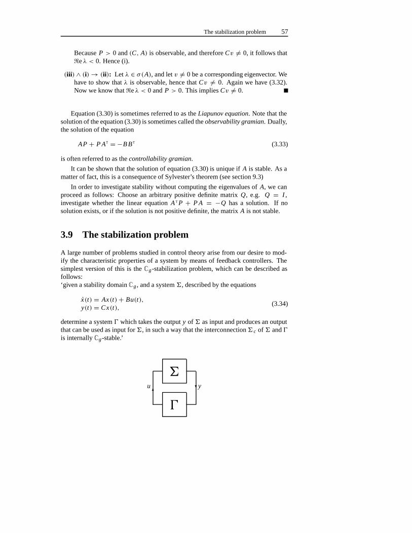
The stabilization problem 57
BecauseP > 0 and(C, A) is observable, and thereforeCv = 0, it follows that�eλ < 0. Hence (i).
(iii ) ∧ (i)→ (ii): Let λ ∈ σ(A), and letv = 0 be a corresponding eigenvector. Wehave to show thatλ is observable, hence thatCv = 0. Again we have (3.32).Now we know that�eλ < 0 andP > 0. This impliesCv = 0.
Equation (3.30) is sometimes referred to as theLiapunov equation. Note that thesolution of the equation (3.30) is sometimes called theobservability gramian. Dually,the solution of the equation
AP + P AT = −B BT (3.33)
is often referred to as thecontrollability gramian.
It can be shown that the solution of equation (3.30) is unique ifA is stable. As amatter of fact, this is a consequence of Sylvester’s theorem (see section 9.3)
In order to investigate stability without computing the eigenvalues ofA, we canproceed as follows: Choose an arbitrary positive definite matrixQ, e.g. Q = I ,investigate whether the linear equationA T P + P A = −Q has a solution. If nosolution exists, or if the solution is not positive definite, the matrixA is not stable.
3.9 The stabilization problem
A large number of problems studied in control theory arise from our desire to mod-ify the characteristic properties of a system by means of feedback controllers. Thesimplest version of this is theCg-stabilization problem, which can be described asfollows:‘given a stability domainCg , and a system�, described by the equations
x(t) = Ax(t)+ Bu(t),y(t) = Cx(t),
(3.34)
determine a system� which takes the outputy of � as input and produces an outputthat can be used as input for�, in such a way that the interconnection� c of� and�is internallyCg-stable.’
�
�
u�
�y
58 Systems with inputs and outputs
In order to write down the equations of the interconnection� c, we combine theequations for� with the equations of thefeedback controller �:
w(t) = Kw(t)+ Ly(t),u(t) = Mw(t) + Ny(t),
(3.35)
Note that we allow a feedthrough term in the output equation. The combination ofthese equations with (3.34) yields the equations of� c:(
x(t)w(t)
)=
(A + B NC B M
LC K
)(x(t)w(t)
)
The interconnection�c is called theclosed-loop system of� and�. In this particularcase,�c is a homogeneous linear system with coefficient matrix
Ae : =(
A + B NC B MLC K
). (3.36)
(The subscript ‘e’ stands for ‘extended’.) So theC g-stabilization problem can bereformulated as:‘given the matrix triple(C, A, B), construct a quadruple(K , L,M, N), such that thematrix Ae defined by (3.36) has all its eigenvalues inCg.’If the matrix quadruple(K , L,M, N) meets this requirement then the controller�
given by (3.35) is calledan internally stabilizing controller for �. In the remainderof this chapter we will study under what conditions an internally stabilizing controllerexists.
3.10 Stabilization by state feedback
A direct solution of the stabilization problem formulated in the previous section isnot so obvious. First we restrict ourselves to the case where the state is available formeasurement, i.e, whereC = I . Also, we only allow astatic feedback as controller.This means that our controller will have the form:u = Fx , for some linear mapF : X → U. When we apply this feedback, i.e., substitute it into the state equationx = Ax + Bu, we obtainx = (A + B F)x . Therefore, the problem of stabilizationby state feedback reads:
‘given a stability domainCg , and mapsA : X→ X, B :U→ X, determine a mapF : X→ U such thatσ(A + B F) ⊂ Cg .’
The solution to this problem is provided by the following celebrated result.
Theorem 3.29 (pole-placement theorem)Let A : X→ X, B : U→ X. Then thereexists for every monic polynomial p(s) of degree n a map F : X → U such thatχA+B F (s) = p(s), if and only if (A, B) is controllable.
For the definition ofχA and the concept of ‘monic’, we refer to section 2.5. Mostof the remainder of this section will be devoted to a proof of this result. Then we willapply it to the stabilization problem.
Stabilization by state feedback 59
Proof of the necessity in theorem 3.29: :If (A, B) is not controllable, there is anuncontrollable eigenvalueλ. For this eigenvalue, there exists a nonzero row vectorη such thatηA = λη, ηB = 0. Then we haveη(A + B F) = λη for all F , henceλ ∈ σ(A + B F) for all F . So, if p(s) is any polynomial such thatp(λ) = 0, theredoes not exist a feedbackF such thatp(s) = χ A+B F (s).
We formulate the proof of this result separately:
Corollary 3.30 If λ is an uncontrollable eigenvalue of (A, B) then λ is an eigenvalueof A + B F for all F.
Before we start with the proof of the sufficiency part we note that we may performa basis transformation(A, B) �→ ( A, B), by A = S−1AS, B = S−1B. If we can findthe desired feedbackF for the transformed system, the matrixF : = F S−1 solves theoriginal problem, sinceA + B F = S( A + B F)S−1 and henceχA+B F = χ A+B F .
Proof of the sufficiency in theorem 3.29 for the casem = 1: :
According to theorem 3.18,(A, B) is isomorphic to a system of the form
A : = A : =
0 1 0 · · · 0
0 0 1. . .
......
.... . .
. . . 00 0 · · · 0 1−an −an−1 · · · −a2 −a1
, b : =
0...
001
. (3.37)
(Herec is irrelevant.) We try to find a feedback matrix for the pair( A, b). The soughtfeedback matrixF is a 1× n matrix, i.e., a row vector. We writef instead ofF :
f = (fn · · · f1
).
It follows that
A + b f =
0 1 0 · · · 0
0 0 1. . .
......
.... . .
. . . 00 0 · · · 0 1
fn − an fn−1 − an−1 · · · f2− a2 f1− a1
which is again a companion matrix with characteristic polynomial
χ A+b f (s) : = sn + (a1− f1)sn−1 + · · · + (an − fn).
If the desired characteristic polynomial is
p(s) = sn + p1sn−1 + · · · + pn,
60 Systems with inputs and outputs
we can choosefk : = ak − pk for k = 1, . . . , n.
In order to prove the multi-input case, we need the following auxiliary result:
Lemma 3.31 If (A, B) is controllable there exist vectors u0, . . . , un−1 such that thevectors defined by
x0 : = 0, xk+1 : = Axk + Buk (k = 0, . . . , n − 1)
are independent.
Proof : Since(A, B) is controllable, we must haveB = 0. Hence,u 0 exists such thatBu0 = 0. Therefore,x1 is independent (as a single vector). Now suppose we havethat x1, . . . , xk are independent. LetL be the space generated byx 1, . . . , xk . Thenext step consists of finding a vectoru k such thatxk+1 : = Axk + Buk ∈ L. If this isnot possible, we must have that
Axk + Bu ∈ L (3.38)
for all u ∈ U. This implies in particular that
Axk ∈ L. (3.39)
Combining (3.38) and (3.39), we findBu ∈ L for all u ∈ U. Hence imB ⊂ L. Inaddition,L is A-invariant. This follows from (3.39) and the fact that fori < k, wehave
Axi = xi+1 − Bui ∈ L.
SinceL is an A-invariant space containing imB, it follows that the inclusion〈A |im B〉 ⊂ L holds. Since(A, B) is controllable, this meansL =X and consequentlyk = n.
Proof of the sufficiency in theorem 3.29: : We first constructu 0, . . . , un−1 andx1, . . . , xn according to the above lemma and we chooseu n arbitrary. There exists a(unique) mapF0 : X → U such thatF0xk = uk for k = 1, . . . , n. Furthermore wedefineb : = Bu0. Then
xk+1 = Axk + B F0xk = (A + B F0)xk
and hencexk = (A + B F0)k−1b for k = 1, . . . , n. Sincex1, . . . , xn are independent
this implies that(A + B F0, b) is controllable. The matrixb consists of one column,so that we may apply the theorem for the casem = 1. This yields a row vectorfsuch thatχA+B F0+bf (s) = p(s). Obviously,F : = F0 + u0 f satisfies the desiredpropertyχA+B F = p.
The pole-placement theorem suggests that the controllability of(A, B) is muchstronger than we actually need for stabilization. The following result expresses anecessary and sufficient condition for stabilization.
State observers 61
Theorem 3.32 Given the matrix pair (A, B) and a stability domain C g, there existsa matrix F such that σ(A + B F) ⊂ Cg if and only if every eigenvalue λ ∈ Cg iscontrollable.
We note that for this result, the conditionCg ∩ R = ∅ is needed (see def. 2.12).For realA, B and F we need some condition that guarantees the existence of realpolynomials of arbitrary degree with zeros inCg . If one allows complex matricesF ,this condition can be omitted.
Proof : The ‘only if’ part is an immediate consequence of corollary 3.30. Now sup-pose that the condition is satisfied. IfB = 0, all eigenvalues are uncontrollable andthe condition implies thatσ(A) ⊂ Cg , so that we can takeF = 0. If (A, B) is con-trollable we choose anyp(s) with zeros inCg and apply the pole-placement theorem.Otherwise we can apply theorem 3.11 to transform(A, B) to a system of the form
A =(
A11 A120 A22
), B =
(B10
).
Eigenvalues ofA22 are uncontrollable and henceσ(A22) ⊂ Cg. We apply the pole-placement theorem to the controllable pair(A 11, B1). Thus we can find a matrixF1such thatσ(A11+ B1F1) ⊂ Cg . Then the matrixF : = (F1 0) satisfies
σ( A + B F) = σ(A11+ B1F1) ∪ σ(A22) ⊂ Cg .
The pair(A, B) is calledstabilizable (or more explicitly,Cg-stabilizable) if thereexists a mapF such thatA + B F is Cg-stable, equivalently, if all uncontrollableeigenvalues are inCg . If Cg has not been specified, ourCg is understood to beC−.
We have assumed up to now that the stabilizing control has the form of a constant,linear, static state feedback. Conceivably, if the conditions of theorem 3.32 are notsatisfied, stabilization might be possible using more general types of stabilizing con-trollers, such as nonconstant (u = F(t)x), nonlinear (u = g(x, t)) or dynamic statefeedback of the type described in section 3.9. However, the following result showsthat if stabilization is possible at all, it can be achieved by means of state feedback asdescribed in theorem 3.32.
Theorem 3.33 If there exists for every x0 an input u ∈ U such that the resulting statex is a Cg-stable Bohl function, then (A, B) is Cg-stabilizable.
Proof : Letλ ∈ σ(A) be uncontrollable and letη = 0 satisfyηA = λη, ηB = 0. If wechoosex0 such thatµ : = ηx0 = 0, the equationx = Ax + Bu implies d
dt ηx = ληx ,and henceηx(t) = eλtµ. There exists an inputu for which x is a Cg-stable Bohlfunction. Then alsoηx must be aCg-stable Bohl function so thatλ ∈ Cg .
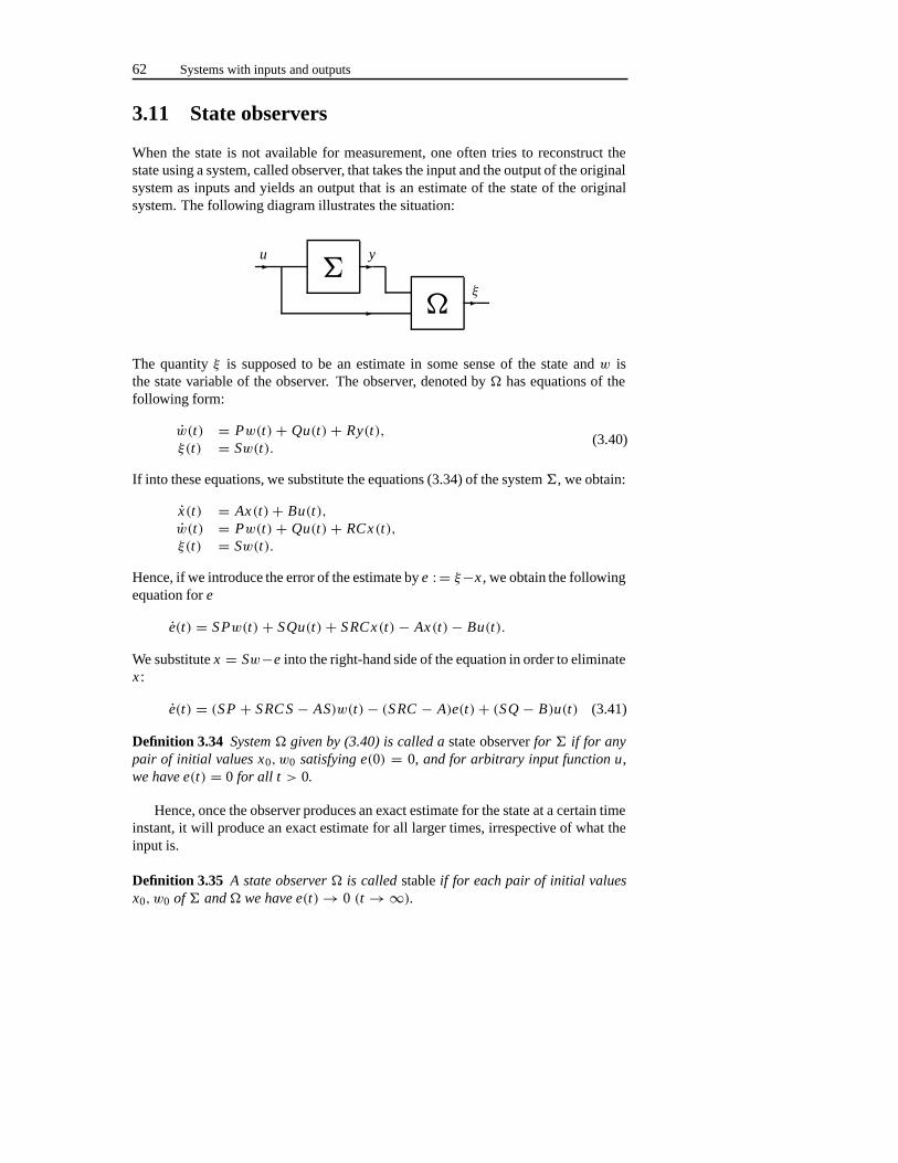
62 Systems with inputs and outputs
3.11 State observers
When the state is not available for measurement, one often tries to reconstruct thestate using a system, called observer, that takes the input and the output of the originalsystem as inputs and yields an output that is an estimate of the state of the originalsystem. The following diagram illustrates the situation:
� � �
���
u y
ξ
The quantityξ is supposed to be an estimate in some sense of the state andw isthe state variable of the observer. The observer, denoted by� has equations of thefollowing form:
w(t) = Pw(t) + Qu(t) + Ry(t),ξ(t) = Sw(t).
(3.40)
If into these equations, we substitute the equations (3.34) of the system�, we obtain:
x(t) = Ax(t)+ Bu(t),w(t) = Pw(t) + Qu(t) + RCx(t),ξ(t) = Sw(t).
Hence, if we introduce the error of the estimate bye : = ξ−x , we obtain the followingequation fore
e(t) = SPw(t) + SQu(t) + SRCx(t) − Ax(t)− Bu(t).
We substitutex = Sw−e into the right-hand side of the equation in order to eliminatex :
e(t) = (SP + SRC S − AS)w(t)− (SRC − A)e(t)+ (SQ − B)u(t) (3.41)
Definition 3.34 System � given by (3.40) is called a state observerfor � if for anypair of initial values x0, w0 satisfying e(0) = 0, and for arbitrary input function u,we have e(t) = 0 for all t > 0.
Hence, once the observer produces an exact estimate for the state at a certain timeinstant, it will produce an exact estimate for all larger times, irrespective of what theinput is.
Definition 3.35 A state observer � is called stableif for each pair of initial valuesx0, w0 of � and� we have e(t)→ 0 (t →∞).
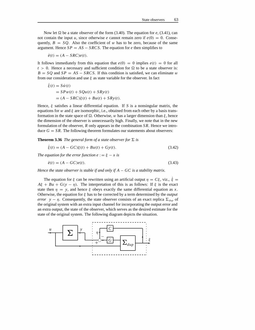
State observers 63
Now let� be a state observer of the form (3.40). The equation fore, (3.41), cannot contain the inputu, since otherwisee cannot remain zero ife(0) = 0. Conse-quently, B = SQ. Also the coefficient ofw has to be zero, because of the sameargument. HenceSP = AS − SRC S. The equation fore then simplifies to
e(t) = (A − SRC)e(t).
It follows immediately from this equation thate(0) = 0 implies e(t) = 0 for allt > 0. Hence a necessary and sufficient condition for� to be a state observer is:B = SQ andSP = AS − SRC S. If this condition is satisfied, we can eliminatewfrom our consideration and useξ as state variable for the observer. In fact
ξ (t) = Sw(t)
= SPw(t) + SQu(t) + SRy(t)
= (A − SRC)ξ(t) + Bu(t)+ SRy(t).
Hence,ξ satisfies a linear differential equation. IfS is a nonsingular matrix, theequations forw andξ are isomorphic, i.e., obtained from each other by a basis trans-formation in the state space of�. Otherwise,w has a larger dimension thanξ , hencethe dimension of the observer is unnecessarily high. Finally, we note that in the newformulation of the observer,R only appears in the combinationSR. Hence we intro-duceG = SR. The following theorem formulates our statements about observers:
Theorem 3.36 The general form of a state observer for � is
ξ (t) = (A − GC)ξ(t)+ Bu(t)+ Gy(t). (3.42)
The equation for the error function e : = ξ − x is
e(t) = (A − GC)e(t). (3.43)
Hence the state observer is stable if and only if A − GC is a stability matrix.
The equation forξ can be rewritten using an artificial outputη = Cξ , viz., ξ =Aξ + Bu + G(y − η). The interpretation of this is as follows: Ifξ is the exactstate thenη = y, and henceξ obeys exactly the same differential equation asx .Otherwise, the equation forξ has to be corrected by a term determined by theoutputerror y − η. Consequently, the state observer consists of an exact replica� dup ofthe original system with an extra input channel for incorporating the output error andan extra output, the state of the observer, which serves as the desired estimate for thestate of the original system. The following diagram depicts the situation.
�u�
�
�y
−+ � G �dup
�ξ�
C�η

64 Systems with inputs and outputs
Obviously, state observers always exist. They are parameterized by the matrixG. Astable state observer exists if and only ifG can be found such thatσ(A − GC)⊂ C−.More generally, one replacesC− by Cg . The problem of finding such aG is dual tothe problem of finding a matrixF to a pair(A, B) such thatA + B F is C g-stable.Hence we are led to the introduction of the dual concept of stabilizability:
Definition 3.37 The pair (C, A) is called Cg-detectableif there exists a matrix Gsuch that σ(A − GC) ⊂ Cg.
Based on the previous considerations and on theorem 3.32 we find the followingresult.
Theorem 3.38 Given system � = (C, A, B), the following statements are equiva-lent:
(i) � has a Cg-stable observer,
(ii) (C, A) is Cg-detectable,
(iii) every (C, A)-unobservable eigenvalue is in Cg.
We have chosen a specific type ofC−-stable state observer, viz., a finite-dimensi-onal, time-invariant, linear system with no feedthrough term. An obvious question isof course, whether in the case of a nondetectable system, for which such an observerdoes not exist, a stable state observer can be constructed of a more general type. Letus call ageneralized state observer any system takingy andu as the only informationabout the state of� and yielding as output an estimateξ of the state with the propertythatξ(t)− x(t)→ 0 (t →∞) for all possibleu. We claim that the existence of suchan observer implies the detectability of�. In fact, suppose thatλ is an unobservableeigenvalue withp = 0 such thatAp = λp and Cp = 0. Assume thatx 0 = 0and u(t) = 0 for all t � 0. Then y(t) = 0 (t > 0). The observer has zeroinput and must yield an outputξ(t) which converges to zero, sincex(t) = 0 andx(t) − ξ(t) → 0 (t → ∞). On the other hand ifx0 = p and still u(t) = 0 for allt , we also havey(t) = 0 and consequently,ξ(t)→ 0, since nothing has changed forthe observer. It follows fromx(t) − ξ(t) → 0 that we must havex(t) → 0. Sincex(t) = eλt p and p = 0, we conclude that�eλ < 0. Hence every unobservableeigenvalue is inC−, so that� is detectable.
As a consequence of our results about state observers, we obtain another conditionfor C−-detectability:
Corollary 3.39 � is C−-detectable if and only if for any initial state and any input,we have: u(t)→ 0 and y(t)→ 0 for t →∞ imply x(t)→ 0 for t →∞.
Proof : (⇒) ChooseG such thatσ(A − GC) ⊂ C−. The state satisfies the equation
x(t) = (A − GC)x(t)+ Bu(t)+ Gy(t),
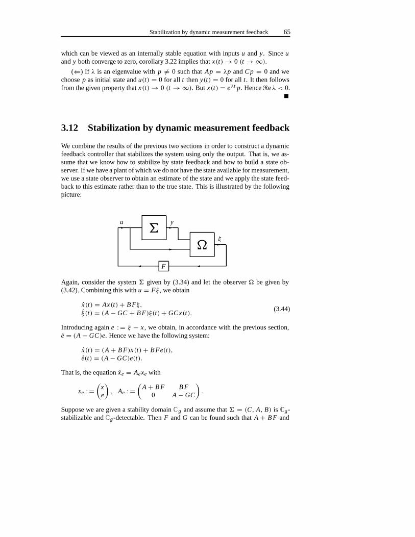
Stabilization by dynamic measurement feedback 65
which can be viewed as an internally stable equation with inputsu and y. Sinceuandy both converge to zero, corollary 3.22 implies thatx(t)→ 0 (t →∞).
(⇐) If λ is an eigenvalue withp = 0 such thatAp = λp andCp = 0 and wechoosep as initial state andu(t) = 0 for all t theny(t) = 0 for all t . It then followsfrom the given property thatx(t)→ 0 (t →∞). But x(t) = eλt p. Hence�eλ < 0.
3.12 Stabilization by dynamic measurement feedback
We combine the results of the previous two sections in order to construct a dynamicfeedback controller that stabilizes the system using only the output. That is, we as-sume that we know how to stabilize by state feedback and how to build a state ob-server. If we have a plant of which we do not have the state available for measurement,we use a state observer to obtain an estimate of the state and we apply the state feed-back to this estimate rather than to the true state. This is illustrated by the followingpicture:
� � �
���
u y
ξ
�F�
Again, consider the system� given by (3.34) and let the observer� be given by(3.42). Combining this withu = Fξ , we obtain
x(t) = Ax(t)+ B Fξ,ξ (t) = (A − GC + B F)ξ(t)+ GCx(t).
(3.44)
Introducing againe : = ξ − x , we obtain, in accordance with the previous section,e = (A − GC)e. Hence we have the following system:
x(t) = (A + B F)x(t)+ B Fe(t),e(t) = (A − GC)e(t).
That is, the equationxe = Aexe with
xe : =(
xe
), Ae : =
(A + B F B F
0 A − GC
).
Suppose we are given a stability domainCg and assume that� = (C, A, B) is Cg-stabilizable andCg-detectable. ThenF andG can be found such thatA + B F and
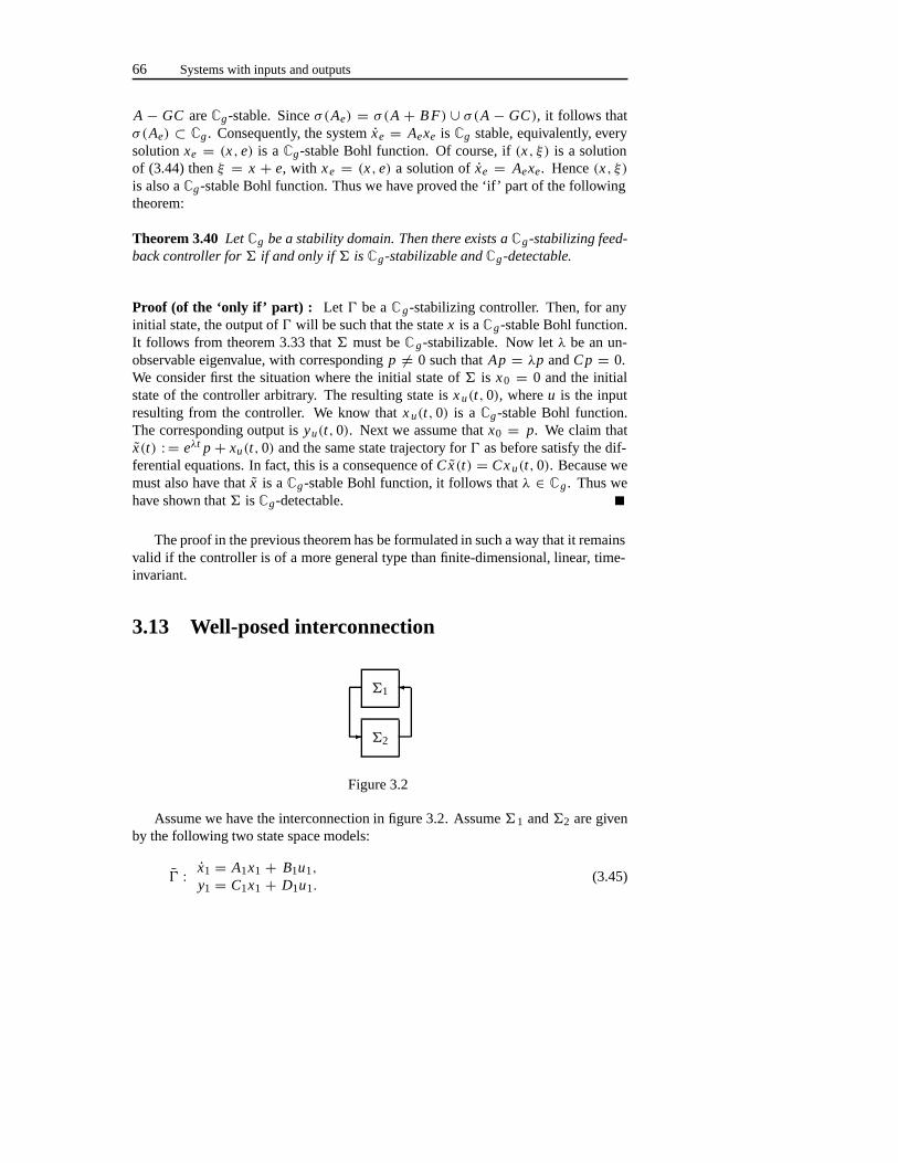
66 Systems with inputs and outputs
A − GC areCg-stable. Sinceσ(Ae) = σ(A + B F) ∪ σ(A − GC), it follows thatσ(Ae) ⊂ Cg . Consequently, the systemxe = Aexe is Cg stable, equivalently, everysolutionxe = (x, e) is aCg-stable Bohl function. Of course, if(x, ξ) is a solutionof (3.44) thenξ = x + e, with xe = (x, e) a solution ofxe = Aexe. Hence(x, ξ)is also aCg-stable Bohl function. Thus we have proved the ‘if’ part of the followingtheorem:
Theorem 3.40 Let Cg be a stability domain. Then there exists a Cg-stabilizing feed-back controller for � if and only if � is Cg-stabilizable and Cg-detectable.
Proof (of the ‘only if’ part) : Let � be aCg-stabilizing controller. Then, for anyinitial state, the output of� will be such that the statex is aCg-stable Bohl function.It follows from theorem 3.33 that� must beCg-stabilizable. Now letλ be an un-observable eigenvalue, with correspondingp = 0 such thatAp = λp andCp = 0.We consider first the situation where the initial state of� is x0 = 0 and the initialstate of the controller arbitrary. The resulting state isx u(t,0), whereu is the inputresulting from the controller. We know thatx u(t,0) is a Cg-stable Bohl function.The corresponding output isyu(t,0). Next we assume thatx0 = p. We claim thatx(t) : = eλt p + xu(t,0) and the same state trajectory for� as before satisfy the dif-ferential equations. In fact, this is a consequence ofCx(t) = Cx u(t,0). Because wemust also have thatx is aCg-stable Bohl function, it follows thatλ ∈ Cg . Thus wehave shown that� is Cg-detectable.
The proof in the previous theorem has be formulated in such a way that it remainsvalid if the controller is of a more general type than finite-dimensional, linear, time-invariant.
3.13 Well-posed interconnection
�1
�2�
�
Figure 3.2
Assume we have the interconnection in figure 3.2. Assume�1 and�2 are givenby the following two state space models:
� : x1 = A1x1 + B1u1,
y1 = C1x1 + D1u1.(3.45)
Exercises 67
and
� : x2 = A2x2 + B2u2,
y2 = C2x2 + D2u2.(3.46)
The interconnection impliesy1 = u2 and y2 = u1. If we try to solve this set ofequations we get:
u2 = y1 = C1x1+ D1u1 = C1x1+ D1(C2x2+ D2u2). (3.47)
and we can solveu2 from the above equation ifI − D1D2 is an invertible matrix. Inthat case the dynamics of the interconnection are given by:(
x1x2
)=
(A1+ B1(I − D2D1)
−1D2C1 B1(I − D2D1)−1C2
B2(I − D1D2)−1C1 A2+ B2(I − D1D2)
−1D1C2
)(x1x2
).
What happens ifI − D1D2 is not invertible? Then there either exist initial statesfor which the equation (3.47) is not solvable foru 2 or there exist multiple solutionsfor u2. Therefore either the interconnection in Figure 3.2 on the facing page has nosolution for certain initial states or the solution exists for for certain initial states butis not unique.
Therefore we call the interconnectionwell posed if for all possible initial statesthe interconnection has a solution which is moreover unique. Otherwise we call theinterconnectionill posed.
We obtain the obvious result that the interconnection in figure 3.2 on the facingpage is well posed if and only ifI − D1D2 is invertible. Note thatI − D1D2 isinvertible if and only ifI − D2D1 is invertible.
In many chapters we will have interconnections where we do not mention the ob-vious requirement that we want to have a well-posed interconnection. This is due tothe fact that the interconnection of a system and a controller is always well posed ifeither the system or the controller is strictly proper. For instance in the previous sec-tion we stabilized the system with a controller which used an observer in combinationwith a state feedback. However, this type of controller is always strictly proper andtherefore the interconnection is always well posed.
3.14 Exercises
3.1 Consider the system� : x = Ax + Bu, y = Cx + Du. If, with x(0) = 0, theoutput is bounded for every input functionu, show that� has transfer functionzero.
3.2 An n× n matrix A is calledcyclic if there exists a column vector (i.e., ann×1matrix) b such that(A, b) is controllable. Show that the following statementsare equivalent:
a. A is cyclic,
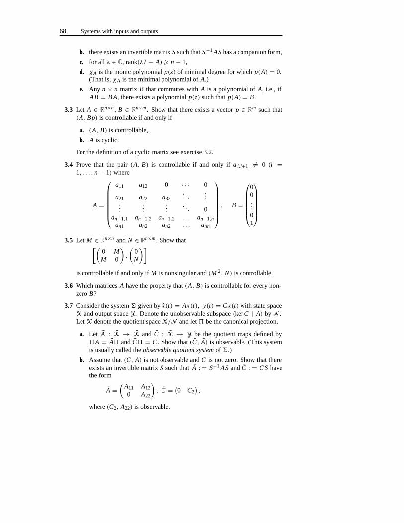
68 Systems with inputs and outputs
b. there exists an invertible matrixS such thatS−1 AS has a companion form,
c. for all λ ∈ C, rank(λI − A) � n − 1,
d. χA is the monic polynomialp(z) of minimal degree for whichp(A) = 0.(That is,χA is the minimal polynomial ofA.)
e. Any n × n matrix B that commutes withA is a polynomial ofA, i.e., ifAB = B A, there exists a polynomialp(z) such thatp(A) = B.
3.3 Let A ∈ Rn×n , B ∈ Rn×m . Show that there exists a vectorp ∈ Rm such that(A, Bp) is controllable if and only if
a. (A, B) is controllable,
b. A is cyclic.
For the definition of a cyclic matrix see exercise 3.2.
3.4 Prove that the pair(A, B) is controllable if and only ifa i,i+1 = 0 (i =1, . . . , n − 1) where
A =
a11 a12 0 · · · 0
a21 a22 a32. . .
......
......
. . . 0an−1,1 an−1,2 an−1,2 . . . an−1,n
an1 an2 an2 . . . ann
, B =
00...
01
3.5 Let M ∈ Rn×n andN ∈ Rn×m . Show that[(0 MM 0
),
(0N
)]
is controllable if and only ifM is nonsingular and(M 2, N) is controllable.
3.6 Which matricesA have the property that(A, B) is controllable for every non-zeroB?
3.7 Consider the system� given byx(t) = Ax(t), y(t) = Cx(t) with state spaceX and output spaceY. Denote the unobservable subspace〈kerC | A〉 by N .Let X denote the quotient spaceX/N and let be the canonical projection.
a. Let A : X → X and C : X → Y be the quotient maps defined byA = A andC = C . Show that(C, A) is observable. (This systemis usually called theobservable quotient system of�.)
b. Assume that(C, A) is not observable andC is not zero. Show that thereexists an invertible matrixS such thatA : = S−1 AS andC : = C S havethe form
A =(
A11 A120 A22
), C = (
0 C2),
where(C2, A22) is observable.
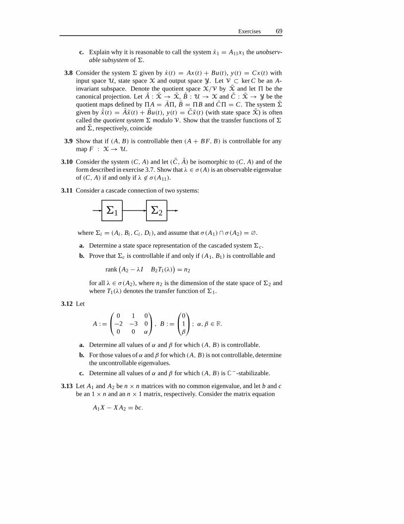
Exercises 69
c. Explain why it is reasonable to call the systemx1 = A11x1 theunobserv-able subsystem of �.
3.8 Consider the system� given by x(t) = Ax(t) + Bu(t), y(t) = Cx(t) withinput spaceU, state spaceX and output spaceY. Let V ⊂ kerC be anA-invariant subspace. Denote the quotient spaceX/V by X and let be thecanonical projection. LetA : X → X, B : U → X andC : X → Y be thequotient maps defined byA = A, B = B andC = C . The system�given by ˙x(t) = Ax(t) + Bu(t), y(t) = C x(t) (with state spaceX) is oftencalled thequotient system � modulo V. Show that the transfer functions of�and�, respectively, coincide
3.9 Show that if(A, B) is controllable then(A + B F, B) is controllable for anymapF : X→ U.
3.10 Consider the system(C, A) and let(C, A) be isomorphic to(C, A) and of theform described in exercise 3.7. Show thatλ ∈ σ(A) is an observable eigenvalueof (C, A) if and only if λ ∈ σ(A11).
3.11 Consider a cascade connection of two systems:
�1 �2� � �
where�i = (Ai , Bi ,Ci , Di ), and assume thatσ(A1) ∩ σ(A2) = ∅.
a. Determine a state space representation of the cascaded system� c.
b. Prove that�c is controllable if and only if(A1, B1) is controllable and
rank(A2− λI B2T1(λ)
) = n2
for all λ ∈ σ(A2), wheren2 is the dimension of the state space of�2 andwhereT1(λ) denotes the transfer function of�1.
3.12 Let
A : = 0 1 0−2 −3 00 0 α
, B : =
0
1β
; α, β ∈ R.
a. Determine all values ofα andβ for which (A, B) is controllable.
b. For those values ofα andβ for which(A, B) is not controllable, determinethe uncontrollable eigenvalues.
c. Determine all values ofα andβ for which (A, B) is C−-stabilizable.
3.13 Let A1 andA2 ben × n matrices with no common eigenvalue, and letb andcbe an 1× n and ann × 1 matrix, respectively. Consider the matrix equation
A1X − X A2 = bc.
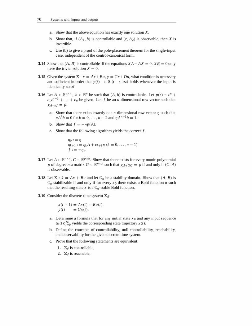
70 Systems with inputs and outputs
a. Show that the above equation has exactly one solutionX .
b. Show that, if(A1, b) is controllable and(c, A2) is observable, thenX isinvertible.
c. Use (b) to give a proof of the pole-placement theorem for the single-inputcase, independent of the control-canonical form.
3.14 Show that(A, B) is controllable iff the equationsX A− AX = 0, X B = 0 onlyhave the trivial solutionX = 0.
3.15 Given the system� : x = Ax+Bu, y = Cx+Du, what condition is necessaryand sufficient in order thaty(t) → 0 (t → ∞) holds whenever the input isidentically zero?
3.16 Let A ∈ Rn×n, b ∈ Rn be such that(A, b) is controllable. Letp(z) = z n +c1zn−1 + · · · + cn be given. Let f be ann-dimensional row vector such thatχA+b f = p.
a. Show that there exists exactly onen-dimensional row vectorη such thatηAkb = 0 for k = 0, . . . , n − 2 andηAn−1b = 1.
b. Show thatf = −ηp(A).
c. Show that the following algorithm yields the correctf .
η0 : = ηηk+1 : = ηk A + ck+1η (k = 0, . . . , n − 1)f : = −ηn.
3.17 Let A ∈ Rn×n , C ∈ Rp×n. Show that there exists for every monic polynomialp of degreen a matrixG ∈ Rn×p such thatχA+GC = p if and only if (C, A)is observable.
3.18 Let � : x = Ax + Bu and letCg be a stability domain. Show that(A, B) isCg-stabilizable if and only if for everyx 0 there exists a Bohl functionu suchthat the resulting statex is aCg-stable Bohl function.
3.19 Consider the discrete-time system�d :
x(t + 1) = Ax(t)+ Bu(t),y(t) = Cx(t).
a. Determine a formula that for any initial statex 0 and any input sequence(u(t))∞t=0 yields the corresponding state trajectoryx(t).
b. Define the concepts of controllability, null-controllability, reachability,and observability for the given discrete-time system.
c. Prove that the following statements are equivalent:
1. �d is controllable,
2. �d is reachable,
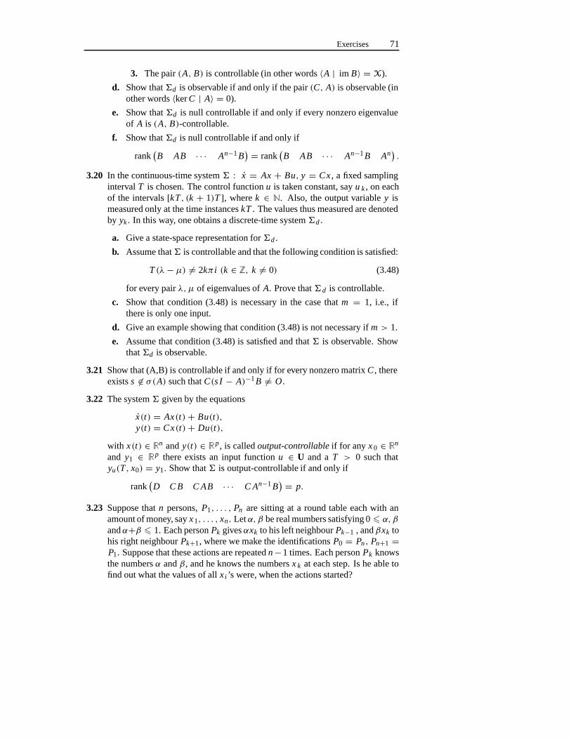
Exercises 71
3. The pair(A, B) is controllable (in other words〈A | im B〉 = X).
d. Show that�d is observable if and only if the pair(C, A) is observable (inother words〈kerC | A〉 = 0).
e. Show that�d is null controllable if and only if every nonzero eigenvalueof A is (A, B)-controllable.
f. Show that�d is null controllable if and only if
rank(B AB · · · An−1B
) = rank(B AB · · · An−1B An
).
3.20 In the continuous-time system� : x = Ax + Bu, y = Cx , a fixed samplingintervalT is chosen. The control functionu is taken constant, sayu k , on eachof the intervals[kT, (k + 1)T ], wherek ∈ N. Also, the output variabley ismeasured only at the time instanceskT . The values thus measured are denotedby yk . In this way, one obtains a discrete-time system�d .
a. Give a state-space representation for�d .
b. Assume that� is controllable and that the following condition is satisfied:
T (λ− µ) = 2kπ i (k ∈ Z, k = 0) (3.48)
for every pairλ,µ of eigenvalues ofA. Prove that� d is controllable.
c. Show that condition (3.48) is necessary in the case thatm = 1, i.e., ifthere is only one input.
d. Give an example showing that condition (3.48) is not necessary ifm > 1.
e. Assume that condition (3.48) is satisfied and that� is observable. Showthat�d is observable.
3.21 Show that (A,B) is controllable if and only if for every nonzero matrixC , thereexistss ∈ σ(A) such thatC(s I − A)−1B = O.
3.22 The system� given by the equations
x(t) = Ax(t)+ Bu(t),y(t) = Cx(t)+ Du(t),
with x(t) ∈ Rn andy(t) ∈ Rp, is calledoutput-controllable if for any x 0 ∈ Rn
and y1 ∈ Rp there exists an input functionu ∈ U and aT > 0 such thatyu(T, x0) = y1. Show that� is output-controllable if and only if
rank(D C B C AB · · · C An−1B
) = p.
3.23 Suppose thatn persons,P1, . . . , Pn are sitting at a round table each with anamount of money, sayx1, . . . , xn . Letα, β be real mumbers satisfying 0� α, β
andα+β � 1. Each personPk givesαxk to his left neighbourPk−1 , andβxk tohis right neighbourPk+1, where we make the identificationsP0 = Pn, Pn+1 =P1. Suppose that these actions are repeatedn−1 times. Each personPk knowsthe numbersα andβ, and he knows the numbersx k at each step. Is he able tofind out what the values of allxi ’s were, when the actions started?
72 Systems with inputs and outputs
3.24 Consider the system� : x = Ax + Bu, with A ∈ Rn×n andB ∈ Rn×m . LetW be the reachable subspace of(A, B), i.e., W = 〈A | im B〉. Define theC−-stabilizable subspace of(A, B) by:
Xstab : = {x0 ∈ Rn | ∃u ∈ U : limt→∞ x(t, x0, u) = 0}.
a. Show thatXstabis a subspace ofRn
b. Show thatW ⊂ Xstab.
c. Find a system� for which the inclusionW ⊂ Xstabis a strict inclusion.
d. Assume that(A, B) is C−-stabilizable. Show thatXstab= Rn .
e. Let λ ∈ C and letη be a nonzero row vector such that
ηA = λη, ηB = 0.
Givenx0 ∈ Rn, u ∈ U, definez : R → C by z(t) : = ηx(t, x0, u). Showthatz satisfies the differential equationz = λz.
f. Show that(A, B) is C−-stabilizable if and only ifXstab= Rn.
3.25 An autonomous discrete-time system�a : x(t + 1) = Ax(t) is called adead-beat system if for any initial valuex0, the statex(t) equals zero fort � n. Whatis a necessary and sufficient condition for the existence of a feedbacku = Fxin the controlled system� : x(t + 1) = Ax(t)+ Bu(t) such that the resulting(autonomous) system is dead-beat?
3.26 Consider the system
x = Ax + Bu (3.49)
and assume thatK ,M, N are matrices satisfyingM � 0, N T = −N, K >
0, AT K + K A < 0. Show that the feedbacku = Fx , whereF : = (N −M)BT K , stabilizes (3.49).
3.27 Let P be a positive semidefinite solution of (3.30) and let(C, A) be observable.Show thatP is positive definite.
3.28 Let n × n matricesA, P, Q satisfy (3.30), and letP > 0, Q � 0. Show that
�(A) � �(−Q)
2�(P).
3.29 Let A be ann × n matrix. If the equationA T P + P A = −I has a positivedefinite solution, then the equationA T P + P A = −Q has a positive solutionfor everyQ > 0.
3.30 (Stabilization algorithm by Bass) Let (A, B) be stabilizable. Show that thefollowing algorithm leads to a stabilizing feedback.
a. Chooseα such that�(−α I − A) < 0, e.g. by takingα > ‖A‖.
Notes and references 73
b. SolveP from the equation
(α I + A)P + P(α I + AT) = 2B BT.
c. ComputeF from F P = −B T.
What can be said about the location of the controllable eigenvalues? Verify inparticular that equations mentioned have a solution.
3.15 Notes and references
The description of linear systems in terms of a state space representation was par-ticularly stressed by R.E. Kalman in the early sixties (see Kalman [91, 93, 94] andKalman, Narendra and Ho [96]). See also Zadeh and Desoer [229], Gilbert [59]). Inparticular, Kalman introduced the concepts of controllability and observability, andgave the conditions expressed in Corollary 3.4, part (iii) and Theorem 3.6, part (v).Also, the decomposition of the state space, given in Theorem 3.11 is due to Kalman.
The concept of controllable and observable eigenvalues was introduced in Hautus[68]. The controllability and observability condition expressed in Theorem 3.13 wereindependently found by a number of authors. The first reference is Popov [148] (seealso [149]). Other references are Belevitch [15] and Rosenbrock [155]. In Hautus[68, 69], the applicability of these conditions are demonstrated. The stabilizabilityand detectability condition of Theorem 3.32 and Theorem 3.38, part (iii), was provedin [69].
The pole-placement was proved in increasing generality by a number of authors:In 1960, J. Rissanen [153] proved the result form = 1 (one input). The result wasgeneralized to the casem > 1 by Popov [147] in 1964. This result was only valid,however, for complex systems. Hence, even if the matricesA, B are real, the re-sulting feedback matrixF could not be guaranteed to be real. A proof valid for realsystems was given in 1967 by Wonham [220]. A drastic simplification in the proofwas obtained by Heymann [77] in 1968. The proof in this chapter was given in Hau-tus [71].
State observers were introduced right with the concept of state-space representa-tion (Kalman [96], Zadeh and Desoer [229]). They were viewed as a deterministic,nonoptimal version of the Kalman filter. The construction of the observer given inthis chapter follows the pattern of the Kalman filters. In the literature, much attentionis spent on reduced observers, i.e., observer with a lower dimensional state space (seeLuenberger [115]).
The results of exercises 3.13 and 3.16 were given in Luenberger [116] and Ack-ermann [1], respectively.

74 Systems with inputs and outputs

Chapter 4
Controlled invariant subspaces
In this chapter we introduce controlled invariant subspaces (which are also called(A, B)-invariant subspaces) and the concepts of controllability subspace and stabiliz-ability subspace. The notion of controlled invariance is of fundamental importancein many of the feedback design problems that the reader will encounter in this book.We will apply these concepts to a number of basic feedback design problems, amongwhich the problem of disturbance decoupling by state feedback. The design prob-lems treated in this chapter have in common that the entire state vector of the controlsystem is assumed to be available for control purposes, and we confine ourselves tothe design of static state feedback control laws. Dynamic feedback will be discussedin chapter 6.
4.1 Controlled invariance
In this section we will introduce the concept of controlled invariant subspace andprove the most important properties of these subspaces. Again consider the system
x(t) = Ax(t)+ Bu(t). (4.1)
The input functionsu are understood to be elements of the classU of admissible inputfunctions (see section 3.1). A subspace of the state space will be called controlledinvariant if it has the following property: for every initial condition in the subspacethere exists an input function such that the resulting state trajectory remains in thesubspace for all times. More explicitly:
Definition 4.1 A subspace V ⊂ X is called controlled invariantif for any x 0 ∈ Vthere exists an input function u such that x u(t, x0) ∈ V for all t � 0.
It follows immediately from the definition that the sum of any number of con-trolled invariant subspaces is a controlled invariant subspace. In order to stress the
76 Controlled invariant subspaces
dependence on the underlying system, we will often use the terminology(A, B)-invariant subspace instead of controlled invariant subspace. It is easily seen that ifF : X → U is a linear map andG : U → U is an isomorphism then a givensubspaceV is (A, B)-invariant if and only if it is(A + B F, BG)-invariant. Stateddifferently: the classes of controlled invariant subspaces associated with the systems(A, B) and(A + B F, BG), respectively, coincide. Sometimes this is expressed bysaying that the property of controlled invariance is invariant under state feedbackand isomorphism of the input space. The following theorem gives several equivalentcharacterizations of controlled invariance:
Theorem 4.2 Consider the system (4.1). Let V be a subspace of X. The followingstatements are equivalent:
(i) V is controlled invariant,
(ii) AV ⊂ V + im B,
(iii) there exists a linear map F : X→ U such that (A + B F)V ⊂ V.
Proof : (i) ⇒ (ii). Let x0 ∈ V and letu be an input function such thatx u(t, x0) ∈ Vfor all t � 0. SinceV is a linear subspace, for allt > 0 we have1
t (xu(t, x0) −x0) ∈ V. Being a subspace ofX, V is closed in the Euclidean topology. Thusx(0+) : = limt↓0
1t (xu(t, x0) − x0) ∈ V. SinceAx0 = x(0+) − Bu(0+) it follows
that Ax0 ∈ V + im B.
(ii) ⇒ (iii). Choose a basisq1, . . . , qn of X adapted toV. For all 1� i � n thereexist vectorsqi ∈ V andui ∈ U such thatAqi = qi + Bui . DefineF : X → Uas follows: for 1� i � k defineFqi : = −ui and fork + 1 � i � n let Fqi bearbitrary vectors inX. Then fori = 1, . . . , k we have(A + B F)q i = qi ∈ V andhence(A + B F)V ⊂ V.
(iii) ⇒ (i). Let x0 ∈ V. We claim that if the system is controlled by the feedbackcontrol lawu = Fx , then the resulting trajectory remains inV. Indeed, using thiscontrol law the trajectoryxu(t, x0) is equal to the solution ofx = (A+B F)x, x(0) =x0. The claim then follows immediately from theorem 2.4.
In the above, the characterization (i) is typically anopen loop characterization:the input functions are allowed to depend on the initial condition arbitrarily. In thisvein, the characterization (iii) is called aclosed-loop characterization: it turns outto be possible to remain within a controlled invariant subspace using a state feed-back control law. As an intermediate between these two we stated (ii), ageometriccharacterization of controlled invariance.
If V is controlled invariant, then we will denote byF(V) the set of all linearmapsF such that(A + B F)V ⊂ V. In the sequel we will often use the notationAF : = A + B F .
Controlled invariance 77
LetV be a controlled invariant subspace and letF ∈ F(V). Consider the equation(4.1). If we represent the controlu asu = Fx + v, we obtain the equation
x(t) = AF x(t)+ Bv(t).
Let x0 ∈ V. We know that if we choosev = 0, then the state trajectory starting inx0 remains inV. We now ask ourselves the question: what other control inputsv
have the property that the resulting state trajectory remains inV? We claim that thetrajectoryx(t) starting inx0 remains inV if and only if Bv(t) ∈ V for all t � 0.Indeed, ifx(t) ∈ V for t � 0, then alsoA F x(t) ∈ V andx(t) ∈ V for t � 0. ThusBv(t) = x(t)− AF x(t) ∈ V for t � 0. Conversely, ifBv(t) ∈ V for t � 0 then
x(t) = eAF t x0+∫ t
0eAF (t−τ )Bv(τ ) dτ ∈ V
for all t � 0, sincee AF t x0 ∈ V for t � 0. Consider the linear subspace
B−1V : = {u ∈ U | Bu ∈ V}.Then Bv(t) ∈ V is equivalent tov(t) ∈ B−1V. Let L be a linear map such thatim L = B−1V. Obviously,v(t) ∈ B−1V for all t � 0 if and only if v(t) =Lw(t), t � 0, for some functionw (compare exercise 2.2). Thus we have proven:
Theorem 4.3 Let V be a controlled invariant subspace. Assume that F ∈ F(V) andlet L be a linear map such that im L = B−1V. Let x0 ∈ V and let u be an inputfunction. Then the state trajectory resulting from x0 and u remains in V for all t � 0if and only if u has the form
u(t) = Fx(t)+ Lw(t) (4.2)
for some input function w.
Note that(AF , B L) can be viewed as the restriction of the system� to the sub-spaceV. After all if we stay insideV thenu must be of the form (4.2). Therefore,the dynamics must be of the form
x(t) = AF x(t)+ B Lw(t).
If K is a subspace ofX which is not controlled invariant, then we are interestedin a controlled invariant subspace contained inK which is as large as possible.
Definition 4.4 Let K be a subspace of X. Then we define
V∗(K) : = {x0 ∈ X | there exists an input function u such that
xu(t, x0) ∈ K for all t � 0}.
78 Controlled invariant subspaces
Two things follow immediately from this definition. First, it is easy to see thatV∗(K) is a linear subspace ofX. Indeed, ifx0, y0 ∈ V∗(K) then there are inputsu andv such thatxu(t, x0) ∈ K andxv(t, y0) ∈ K for all t � 0. Let λ,µ ∈ R.Definew(t) : = λu(t)+µv(t). Thenxw(t, λx0+µy0) ∈ K for all t � 0 (see (3.2)).Secondly, it is clear thatV∗(K) ⊂ K. In fact, we have the following result:
Theorem 4.5 Let K be a subspace of X. Then V ∗(K) is the largest controlledinvariant subspace contained in K , i.e.
(i) V∗(K) is a controlled invariant subspace,
(ii) V∗(K) ⊂ K ,
(iii) if V ⊂ K is a controlled invariant subspace then V ⊂ V ∗(K).
Proof : We first show thatV∗(K) is controlled invariant. Assumex0 ∈ V∗(K).There is an inputu such thatxu(t, x0) ∈ K for all t � 0. We claim that, in fact,xu(t, x0) ∈ V∗(K) for all t � 0. To show this, take a fixed but arbitraryt1 � 0.Let x1 : = xu(t1, x0). It will be shown thatx1 ∈ V∗(K). Indeed, if we definev(t) : = u(t1 + t) (t � 0), then using (3.2) we havex v(t, x1) = xu(t + t1, x0) ∈ Kfor all t � 0. This proves thatx1 = xu(t1, x0) lies in V∗(K). Sincet1 was arbitrary,xu(t, x0) ∈ V∗(K) for all t � 0 and henceV ∗(K) is controlled invariant.
Next, we show thatV∗(K) is the largest controlled invariant subspace inK.Let V ⊂ K be controlled invariant. Letx0 ∈ V. There is an inputu such thatxu(t, x0) ∈ V for all t � 0. Consequently,xu(t, x0) ∈ K for all t � 0 and hencex0 ∈ V∗(K). This completes the proof.
In order to display the dependence on the underlying system we will sometimesdenoteV∗(K) by V∗(K, A, B).
4.2 Disturbance decoupling
Consider the system
x(t) = Ax(t)+ Ed(t),z(t) = H x(t).
(4.3)
In the differential equation above,d represents an unknown disturbance which isassumed to be an element of a given function space. For a given initial conditionx 0and disturbanced, the output of the system is given by
z(t) = H eAt x0+∫ t
0T (t − τ )d(τ ) dτ. (4.4)
HereT (t) : = H eAt E is the impulse response between the disturbance and the out-put. The system (4.3) will be calleddisturbance decoupled if T = 0 or, equivalently,
Disturbance decoupling 79
if the transfer functionG(s) = H (I s− A)−1E is equal to zero. If this is the case thenfor any given initial conditionx0 the output is equal toz(t) = H e At x0 for all distur-bancesd. This means that in a system which is disturbance decoupled, the outputdoes not depend on the disturbance. The following theorem will play an importantrole in the sequel:
Theorem 4.6 The system (4.3) is disturbance decoupled if and only if there exists anA-invariant subspace V such that im E ⊂ V ⊂ kerH .
Proof : (⇒) If T = 0 then also all its time derivativesT (k) are identically equal to0. Thus,T (k)(t) = H AkeAt E = 0 for all t . By taking t = 0 this yieldsH Ak E =0, k = 0,1,2, . . . DefineV : = im
(E AE · · · An−1E
). ThenV ⊂ kerH .
By corollary 3.3,V is equal to〈A | im E〉, the smallestA-invariant subspace thatcontains imE .
(⇐) If im E ⊂ V andV is A-invariant, then also imA k E ⊂ V for k = 0,1,2, . . ..Since we know thatV ⊂ kerH this yields H Ak E = 0 for all k. Thus T (t) =∑∞
k=0(tk/k!)H Ak E = 0 for all t . It follows that the system is disturbance decoupled.
If the system (4.3) is not disturbance decoupled, then one can try tomake it dist-urbance decoupled. In order to do this one needs the possibility to change the sys-tem’s dynamics by using a control input. This possibility is modelled by adding acontrol term to the right hand side of the original differential equation in (4.3). Thuswe consider the system
x(t) = Ax(t)+ Bu(t)+ Ed(t),z(t) = H x(t).
(4.5)
In this description, the variableu represents a control input (see also section 2.8). LetF : X → U be a linear map. If in (4.5) we substituteu(t) = Fx(t), the system’sequations change into
x(t) = (A + B F)x(t)+ Ed(t),z(t) = H x(t),
(4.6)
the closed-loop system obtained from the state feedback control lawu = Fx . Theimpulse response matrix of (4.6) is called theclosed-loop impulse response and isequal to
TF (t) : = H e(A+B F)t E .
The corresponding transfer functionG F (s) : = H (I s − A − B F)−1E is called theclosed-loop transfer function. The problem of disturbance decoupling by state feed-back is to find a linear mapF : X → U such that the closed-loop system (4.6) isdisturbance decoupled:
80 Controlled invariant subspaces
Definition 4.7 Consider the system (4.3). The problem of disturbance decoupling bystate feedback, DDP, is to find a linear map F : X → U such that TF = 0 (or,equivalently, such that G F = 0).
The following result establishes the connection between the concept of controlledinvariance and the problem of disturbance decoupling.
Theorem 4.8 There exists a linear map F : X → U such that TF = 0 if and only ifthere exists a controlled invariant subspace V such that im E ⊂ V ⊂ kerH.
Proof : (⇒) If TF = 0 then (4.6) is disturbance decoupled. By theorem 4.6 there isan(A+ B F)-invariant subspaceV such that imE ⊂ V ⊂ kerH . By theorem 4.2,Vis controlled invariant.
(⇐) Let V be a controlled invariant subspace such that imE ⊂ V ⊂ kerH . Bytheorem 4.2 there exists a linear mapF : X→ U such thatV is (A+ B F)-invariant.It then follows from theorem 4.6 that the system (4.6) is disturbance decoupled.
Corollary 4.9 There exists a linear map F : X→ U such that TF = 0 if and only if
im E ⊂ V∗(kerH ). (4.7)
Formula (4.7) provides a very compact necessary and sufficient condition for theexistence of a state feedback control law that achieves disturbance decoupling. How-ever, in order to be able to check this condition for an actual system, we would liketo have an algorithm. In the next section we will describe an algorithm that, startingfrom a system (4.5), calculates the associated subspaceV ∗(kerH ).
4.3 The invariant subspace algorithm
In this section we give an algorithm to compute the subspaceV ∗(K). Consider thesystem(A, B) and letK be a subspace of the state spaceX. The algorithm we giveis most easily understood if one thinks in terms of the discrete-time system
xt+1 = Axt + But , t = 0,1,2, . . . . (4.8)
Given an input sequenceu = (u 0, u1, u2, . . .) and an initial conditionx0, the resultingdiscrete-time state trajectory is denoted byx = (x0, x1, x2, . . .). The discrete-timeanalogueV∗d (K) of the subspaceV∗(K) defined by definition 4.4 is obviously thesubspace of allx0 ∈ X for which there exists an input sequenceu such that all termsof the resulting state trajectory lie inK:
V∗d (K) : = {x0 ∈ X | there is an input sequenceu such that
xt ∈ K for t = 0,1,2, . . .}.
The invariant subspace algorithm 81
Define a sequence of subspacesV0,V1,V2, . . . by
Vt : = {x0 ∈ X | there is an input sequenceu such thatx0, x1, x2, . . . , xt ∈K}.Thus,Vt consists of those points in which a state trajectory starts for which the firstt + 1 terms lie inK. It is easily verified thatVt is indeed a subspace, thatV0 = Kand thatV0 ⊃ V1 ⊃ V2 ⊃ · · · . It turns out to be possible to derive a recurrencerelation forVt . Indeed,x0 ∈ Vt+1 if and only if x0 ∈K and there existsu0 ∈ U suchthat Ax0+ Bu0 ∈ Vt . Hence,x0 ∈ Vt+1 if and only if x0 ∈K andAx0 ∈ Vt + im Bor, equivalently,x0 ∈ A−1(Vt + im B). It follows that
V0 = K, Vt+1 = K ∩ A−1(Vt + im B). (4.9)
From this recurrence relation it follows immediately that ifVk = Vk+1 for somek,thenVk = Vt for all t � k. Now, recall thatV0 ⊃ V1 ⊃ V2 ⊃ · · · . If we have strictinclusion, the dimension must decrease by at least one. Hence the inclusion chainmust have the form
V0 ⊃ V1 ⊃ · · · ⊃ Vk = Vk+1 = Vk+2 = · · ·for some integerk � dimK (� n − 1). In the above formula,⊃ stands forstrictinclusion. We claim thatV∗d (K) = Vk . Indeed, on the one hand it follows immedi-ately from the definition thatV ∗
d (K) ⊂ Vt for all t . Conversely, assumex0 ∈ Vk .We want to construct an input sequence(u 0, u1, . . .) such that the correspondingstate trajectoryx = (x0, x1, . . .) lies in K. Since x0 ∈ Vk = Vk+1, there isu0 such thatx1 = Ax0 + Bu0 ∈ Vk . Thus, in particular we havex0, x1 ∈ K.We now proceed inductively. Assumeu 0, u1, . . . , us−1 have been found such thatx0, x1, . . . , xs−1 ∈ K, while xs ∈ Vk . Again usingVk = Vk+1 we can findus suchthatxs+1 = Axs + Bus ∈ Vk . This proves our claim.
The above is meant to provide some intuitive background for the introduction ofthe recurrence relation (4.9). This recurrence relation will henceforth be calledtheinvariant subspace algorithm, ISA. Of course, we still have to show its relevance incontinuous-time systems. In the following result we will collect the properties of thesequence{Vt } we established above and prove that it can be used to calculate thelargest controlled invariant subspace contained inK for the continuous-time system(4.1).
Theorem 4.10 Consider the system (4.1). Let K be a subspace of X. Let V t , t =0,1,2, . . ., be defined by the algorithm (4.9). Then we have
(i) V0 ⊃ V1 ⊃ V2 ⊃ · · · ,(ii) there exists k � dimK such that Vk = Vk+1,
(iii) if Vk = Vk+1 then Vk = Vt for all t � k,
(iv) if Vk = Vk+1 then V∗(K) = Vk .
82 Controlled invariant subspaces
Proof : The statements (i), (ii) and (iii) were proven above. To prove (iv), note thatVk ⊂ K. Moreover, it follows immediately from (4.9) that
AVk = AVk+1 ⊂ Vk + im B.
HenceVk is a controlled invariant subspace contained inK and therefore containedin V∗. To prove the converse inclusion, we show that in factV ∗ ⊂ Vt for all t .Obviously this is true fort = 0. AssumeV ∗ ⊂ Vt−1. SinceV∗ is controlledinvariant we haveAV∗ ⊂ V∗ + im B. ThusAV∗ ⊂ Vt−1 + im B and henceV∗ ⊂A−1(Vt−1+ im B). Finally,V∗ ⊂K so we conclude thatV∗ ⊂ Vt .
Of course item (iv) is crucial because it tells us that there exists afinite algorithmto computeV∗. As a matter of fact it is easily seen that we need at mostn steps wheren is the dimension of the state space.
4.4 Controllability subspaces
Consider the system (4.1). If a subspace of the state space has the property that everypoint in that subspace can be steered to the origin in finite time without leaving thesubspace, it is called a controllability subspace.
Definition 4.11 A subspace R ⊂ X is called a controllability subspaceif for everyx0 ∈ R there exists T > 0 and an input function u such that x u(t, x0) ∈ R for0 � t � T and xu(T, x0) = 0.
It is immediately clear from this definition that every controllability subspace iscontrolled invariant. Indeed, if one chooses the control input to be equal to zero fort > T , the state trajectory also remains zero and hence does not leaveR. As was thecase with controlled invariant subspaces, it can be shown that the sum of any (finite orinfinite) number of controllability subspaces is a controllability subspace. Also, theclass of all controllability subspaces associated with a given system is invariant understate feedback and isomorphisms of the input space. That is, ifR is a controllabilitysubspace with respect to(A, B), it is a controllability subspace with respect to(A +B F, BG) for all linear mapsF : X→ U and isomorphismsG of U.
We can give the following characterization of controllability subspaces:
Theorem 4.12 A subspace R ⊂ X is a controllability subspace if and only if thereexist linear maps F and L such that
R = 〈A + B F | im B L〉. (4.10)
Proof : (⇒) Let F ∈ F(R) and L be a linear map such that imL = B −1R. Weclaim that (4.10) holds. Letx0 ∈ R. There isT > 0 and an inputu such thatxu(t, x0) ∈ R for all t � 0 andxu(T, x0) = 0. By theorem 4.3 there existsw such
Controllability subspaces 83
thatu(t) = Fxu(t, x0) + Lw(t). Hence,xu(t, x0) is a state trajectory of the systemx(t) = AF x(t) + B Lw(t) with state spaceR. Along this trajectory,x0 is steered to0 at timet = T . Since this is possible for allx0 ∈ R, it follows that the latter systemis null-controllable. Consequently, it is reachable soR = 〈A F | im B L〉 (see section3.2).
(⇐) Assume that (4.10) holds. Then we haveA FR ⊂ R and imB L ⊂ R. Thusx(t) = AF x(t) + B Lw(t) defines a system with state spaceR. By corollary 3.4,this system is controllable. Hence every point inR can be controlled to the origin infinite time while remaining inR.
It follows from the proof of the above theorem that ifR is a controllabilitysubspace then for the mapsF and L in the representation (4.10) we can take anyF ∈ F(R) and any mapL such that imL = B−1R. Since the latter equality impliesim B L = im B ∩R we obtain the following:
Corollary 4.13 Let R be a controllability subspace. Then for any F ∈ F(R) wehave
R = 〈A + B F | im B ∩R〉.
If K is a subspace of the state spaceX then we are interested in the largestcontrollability subspace that is contained inK (see also definition 4.4).
Definition 4.14 Let K be a subspace of X. Then we define
R∗(K) : = {x0 ∈ X | there exists an input function u and T > 0 such that
xu(t, x0) ∈K for all 0 � t � T and xu(T, x0) = 0}.
Clearly,R∗(K) is contained inK. In fact, we have
Theorem 4.15 Let K be a subspace of X. Then R∗(K) is the largest controllabilitysubspace contained in K , i.e.
(i) R∗(K) is a controllability subspace,
(ii) R∗(K) ⊂ K ,
(iii) if R ⊂ K is a controllability subspace then R ⊂ R∗(K).
Proof : We first show thatR∗(K) is a subspace. Letx0, y0 ∈ R∗(K) andλ,µ ∈R. There exist controlsu, v and numbersT1, T2 > 0 such thatxu(T1, x0) = 0,xv(T2, y0) = 0, xu(t, x0) ∈ K for all 0 � t � T1 and xv(t, y0) ∈ K for all0 � t � T2. Without loss of generality, assume thatT1 � T2. Define a new controlfunctionu by u(t) = u(t) (0 � t � T1) andu(t) = 0 (t > T1). Thenxu(T2, x0) = 0andxu(t, x0)(t) ∈ K for all 0 � t � T2. Define noww(t) : = λu(t) + µv(t). Thenxw(T2, λx0 + µy0) = 0 andxw(t, λx0+ µy0) ∈K for all 0 � t � T2.
84 Controlled invariant subspaces
Next, we prove thatR∗(K) is a controllability subspace. Letx0 ∈ R∗(K). Thereis a control inputu and a numberT > 0 such thatx u(T, x0) = 0 andxu(t, x0) ∈ Kfor all 0 � t � T . We contend that, in fact,xu(t, x0) ∈ R∗(K). To prove this,take a fixed but arbitraryt1 < T . Let x1 : = xu(t1, x0). Define a new input functionv by v(t) : = u(t + t1) (t � 0). Then xv(t, x1) = xu(t1 + t, x0) ∈ K for all0 � t � T − t1 and xv(T − t1, x1) = xu(T, x0) = 0. Consequently,x1 can becontrolled to the origin in finite time while remaining inK and hencex 1 ∈ R∗(K).Sincet1 was arbitrary we find thatxu(t, x0) ∈ R∗(K) for all 0 � t � T . Finally,the fact thatR∗(K) is the largest controllability subspace inK is proven completelysimilarly as the corresponding part of theorem 4.5.
Sometimes, we will denoteR∗(K) by R∗(K, A, B). Starting with a subspaceK of the state space, we have now definedV ∗(K) (see definition 4.4) andR∗(K).SinceR∗(K) is controlled invariant and contained inK, it must be contained in thelargest controlled invariant subspace inK. Thus
R∗(K) ⊂ V∗(K) ⊂K. (4.11)
More specifically, we haveR∗(V∗(K)) = R∗(K). In the following, whenever thisis convenient, we denoteR∗(K) andV∗(K) by R∗ andV∗, respectively.
Lemma 4.16 Let K be a subspace of X. Then im B ∩V ∗(K) ⊂ R∗(K).
Proof : Let L be a linear map such that imL = B−1V∗. Then imB L = im B ∩ V∗.ChooseF ∈ F(V∗). Then we have
im B ∩ V∗ ⊂ 〈AF | im B L〉 ⊂ V∗ ⊂ K.
Since〈AF | im B L〉 is a controllability subspace (see theorem 4.12) it must be con-tained inR∗(K). This proves the lemma.
The above lemma will be used to prove the following, stronger, result:
Theorem 4.17 Let K be a subspace of X. Then F(V ∗) ⊂ F(R∗) and
R∗ = 〈A + B F | im B ∩ V∗〉 (4.12)
for all F ∈ F(V∗).
In the above,F(R∗) denotes the set of all linear mapsF with the property thatR ∗is A+ B F invariant. This is consistent with our earlier notationF(V) with respect tothe controlled invariant subspaceV, since every controllability subspace is controlledinvariant.
Pole placement under invariance constraints 85
Proof : Let F ∈ F(V∗). SinceR∗ ⊂ V∗ we have thatAFR∗ ⊂ V∗. On the otherhand, sinceR∗ is controlled invariant,A FR∗ ⊂ R∗ + im B. Thus we have
AFR∗ ⊂ (im B +R∗) ∩ V∗ = (im B ∩ V∗)+R∗ ⊂ R∗.
where we used the modular rule for the equality in the middle. This shows thatF ∈ F(R∗). Next, by corollary 4.13,R∗ = 〈AF | im B ∩R∗〉. Moreover, it followsfrom lemma 4.16 that imB ∩ R∗ = im B ∩ V∗. This completes the proof of thetheorem.
The above theorem has the following interpretation. By takingF ∈ F(V ∗) and alinear mapL such that imL = B−1V∗ we obtain a new system
x(t) = (A + B F)x(t)+ B Lw(t)
with state spaceV∗. This system can be considered as being obtained from the orig-inal system by restricting the trajectories to the subspaceV ∗ and by restricting theinput functions to take their values inB−1V∗. Since imB L = im B ∩ V∗, (4.12)expresses the fact thatR∗ is just the reachable subspace of this restricted system.
If V is a controlled invariant subspace then of courseV = V ∗(V). Let R : =R∗(V), the largest controllability subspace contained inV. Then theorem 4.17 saysthat if F ∈ F(V) andL is a linear map such that imL = B−1V then
R = 〈A + B F | im B L〉. (4.13)
Finally we note that it follows from theorem 4.17 thatR ∗(X), the largest controlla-bility subspace of the system (4.1), is equal to the reachable subspace〈A | im B〉. In-deed, the state spaceX itself is of course a controlled invariant subspace soV ∗(X) =X andF(X) = {F : X→ U | F is linear}. It also follows from this that every con-trollability subspaceV is contained in〈A | im B〉.
4.5 Pole placement under invariance constraints
In section 3.10 we have discussed to what extent one can assign the spectrum of thesystem map using state feedback. In section 4.1 we introduced the class of controlledinvariant subspaces and showed that these are characterized by the property that theycan be made invariant by state feedback. In the present section we will combinethese two issues and ask ourselves the question: how much freedom is left in theassignment of the spectrum of the system map if it is required that a given controlledinvariant subspace should be made invariant? More concretely: given a controlledinvariant subspaceV, what freedom do we have in the assignment of the spectrum ofA+ B F if we restrict ourselves toF ∈ F(V). The following result gives a completesolution.
Theorem 4.18 Consider the system (4.1). Let V be a controlled invariant subspace.Let R : = R∗(V) be the largest controllability subspace contained in V. Let S : =V + 〈A | im B〉. Then we have
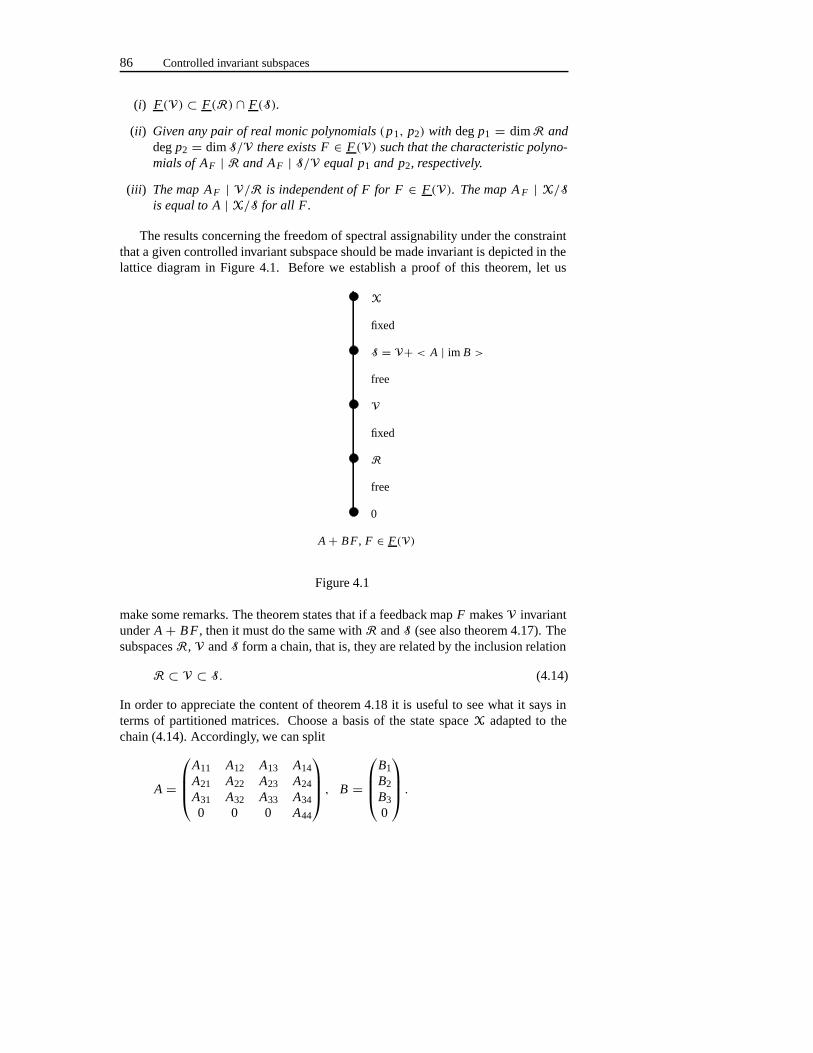
86 Controlled invariant subspaces
(i) F(V) ⊂ F(R) ∩ F(S).
(ii) Given any pair of real monic polynomials (p1, p2) with degp1 = dimR anddegp2 = dimS/V there exists F ∈ F(V) such that the characteristic polyno-mials of AF | R and AF | S/V equal p1 and p2, respectively.
(iii) The map AF | V/R is independent of F for F ∈ F(V). The map A F | X/Sis equal to A | X/S for all F.
The results concerning the freedom of spectral assignability under the constraintthat a given controlled invariant subspace should be made invariant is depicted in thelattice diagram in Figure 4.1. Before we establish a proof of this theorem, let us
X
fixed
A + B F, F ∈ F(V)
0
S = V+ < A | im B >
free
V
fixed
R
free
Figure 4.1
make some remarks. The theorem states that if a feedback mapF makesV invariantunderA + B F , then it must do the same withR andS (see also theorem 4.17). ThesubspacesR, V andS form a chain, that is, they are related by the inclusion relation
R ⊂ V ⊂ S. (4.14)
In order to appreciate the content of theorem 4.18 it is useful to see what it says interms of partitioned matrices. Choose a basis of the state spaceX adapted to thechain (4.14). Accordingly, we can split
A =
A11 A12 A13 A14A21 A22 A23 A24A31 A32 A33 A340 0 0 A44
, B =
B1B2B30
.
Pole placement under invariance constraints 87
Here, the zero blocks appear due to the facts that the subspaceS is A-invariant andcontains the subspace imB. A mapF = (
F1 F2 F3 F4)
is an element ofF(V)if and only if
A31+ B3F1 = 0 and A32+ B3F2 = 0. (4.15)
If we restrict ourselves to mapsF satisfying (4.15) then automaticallyA 21+ B2F1 =0 (see theorem 4.17). Theorem 4.18 asserts that, under the restriction thatF1 shouldsatisfy (4.15), the spectrum ofA11+ B1F1 is freely assignable. Also, the eigenvaluesof A33 + B3F3 can be placed arbitrarily by appropriate choice ofF3. Finally, thetheorem states that, under the restriction (4.15) onF2, the mapA22+ B2F2 is fixed.More specifically, ifF 1
2 and F22 satisfy A32 + B3Fi
2 = 0 (i = 1,2) then we haveA22+ B2F1
2 = A22+ B2F22 and, a fortiori, alsoσ(A22+ B2F1
2 ) = σ(A22+ B2F22 ).
The blockA44 is not affected by any feedback mapF and consequently alsoσ(A 44)
is fixed.
As a consequence of the above theorem, given a pair of real monic polynomials(p1, p2) with degp1 = dimR and degp2 = dimS/V, we can find a linear map(F1 F2 F3 F4) = F ∈ F(V) such that the characteristic polynomial ofA + B Fbecomes equal to the productp1 · q · p2 · r . Hereq is equal to the characteristicpolynomial of A22+ B2F2 which, as noted before, is the same for all mapsF2 suchthat F ∈ F(V). The polynomialr is equal to the characteristic polynomial ofA 44.
In the proof of theorem 4.18 the following lemma will be useful.
Lemma 4.19 Let V be a controlled invariant subspace and let F0 ∈ F(V). LetF : X→ U be a linear map. Then F ∈ F(V) if and only if (F0 − F)V ⊂ B−1V.
Proof : (⇒) Let x0 ∈ V. Then(A + B F0)x0 ∈ V and(A + B F)x0 ∈ V. HenceB(F0 − F)x0 ∈ V.
(⇐) Let x0 ∈ V. ThenB(F0 − F)x0 ∈ V. Also (A + B F0)x0 ∈ V. It followsthat also(A + B F)x0 = (A + B F0)x0− B(F0− F)x0 ∈ V.
We will now give a proof of theorem 4.18.
Proof of theorem 4.18: : (i) The fact thatF(V) ⊂ F(R) was already provenin theorem 4.17. The subspaceS is invariant underA + B F for any F (see alsoexercise 4.2).
(ii) Let (p1, p2) be a pair of polynomials as in the statement of the theorem. Wechoose anyF0 ∈ F(V) andL : Rk → U with im L = B−1V, wherek : = dim B−1V.Then, according to (4.13), we have
R = 〈A + B F0 | im B L〉.DefineA0 : = (A + B F0) | R andB0 : = B L. Then the system(A0, B0) is controll-able (see corollary 3.4) and hence, by theorem 3.29, there exists a mapF 1 : R → Rk
88 Controlled invariant subspaces
such thatA0 + B0F1 has characteristic polynomialp1. ExtendF1 to a linear mapfrom X → Rk . DefineF2 : = F0 + L F1. SinceF2 − F0 = L F1 and imL = B−1V,it follows from lemma 4.19 thatV is invariant underA+ B F2. Also S is (A+ B F2)-invariant. Let : S → S/V be the canonical projection (see section 2.4). DefineA2 : = (A+B F2) | S/V and letB2 :U→ S/V be defined byB2 : = B. We claimthat the system(A2, B2) is controllable. We will show thatS/V = 〈A2 | im B2〉. Letx ∈ S/V, say x = x with x ∈ S. Thenx can be written asx = x1 + x2 withx1 ∈ 〈A | im B〉 = 〈A + B F2 | im B〉 andx2 ∈ V. SinceV = ker we have that infact x = x1. There areu0, . . . , un−1 ∈ U such thatx1 =∑
i (A+ B F2)i Bui . Thus
x = x1 =∑
i
(A + B F2)i Bui
=∑
i
Ai2B2ui ∈ 〈A2 | im B2〉.
Here, we have used the fact that(A + B F2) = A2 andB2 = B. This provesour claim. Now, by theorem 3.29 there exists a mapF3 : S/V → U such thatthe characteristic polynomial ofA2 + B2F3 equalsp2. Define F3 : S → U byF3 : = F3 and extendF3 to a map onX. DefineF : = F2+F3. Then(A+B F)V =(A + B F2)V ⊂ V so F ∈ F(V). Also, (A + B F) | S/V = A2+ B2F3 since
(A2+ B2F3) = A2+B F3 = (A + B F2)+B F3 = (A+ B F).
Thus, the characteristic polynomial of(A + B F) | S/V is equal top2. It remainsto be shown that the characteristic polynomial of(A + B F) | R equalsp 1. Thishowever follows from the fact that(A + B F) | R = A0+ B0F1.
(iii) Let F1, F2 ∈ F(V). According to lemma 4.19 we have(F1−F2)V ⊂ B−1V.HenceB(F1− F2)V ⊂ V∩ im B ⊂ R (see lemma 4.16). Let1 : V → V/R be thecanonical projection. SinceR = ker1 we have1B(F1− F2)V = 0. DenoteA1 := (A+B F1) | V/R andA2 : = (A+B F2) | V/R. Let x ∈ V/R, sayx = 1x withx ∈ V. Then(A1− A2)x = (A11− A21)x = (1(A+ B F1)−1(A+ B F2))x= 1B(F1 − F2)x = 0. ThusA1 = A2 and hence the map(A + B F) | V/R isindependent ofF for F ∈ F(V).
Finally, let2 : X → X/S be the canonical projection. Since imB ⊂ S andS = ker2 we have2B = 0. Let F1, F2 be linear mapsX → U. Note thatS is(A + B Fi )-invariant(i = 1,2) and defineAi : = (A + B Fi ) |X/S. Let x ∈ X/S,sayx = 2x . Then(A1− A2)x = (A12− A22)x = (2(A + B F1)−2(A +B F2))x = 2B(F1 − F2)x = 0. ThusA1 = A2 and(A + B F) | X/S = A | X/Sfor everyF .
We close this section by applying theorem 4.18 to obtain the following character-ization of controllability subspaces.
Theorem 4.20 Consider the system (4.1). Let V be a subspace of X. The followingstatements are equivalent:
Stabilizability subspaces 89
(i) V is a controllability subspace,
(ii) for all for all λ ∈ C we have (λI − A)V + im B = V + im B,
(iii) for each real monic polynomial p with degp = dimV, there exists F ∈ F(V)such that the characteristic polynomial of A F | V equals p.
Proof : (i) ⇒ (iii). Follows by applying theorem 4.18 to the subspaceV. Note thatR∗(V) = V.
(iii) ⇒ (ii). From the fact thatF(V) = ∅ it follows thatV is controlled invariant.HenceAV ⊂ V + im B (see theorem 4.2) and consequently(λI − A)V + im B ⊂V + im B for all λ ∈ C. To prove the converse inclusion it suffices to show thatV ⊂ (λI − A)V + im B for all λ. Let λ ∈ C. Pick a real monic polynomialp withdegp = dimV such thatp(λ) = 0. There isF ∈ F(V) such that the characteristicpolynomial of A F | V equalsp. It follows thatλ ∈ σ(A + B F | V) so the map(λI − A− B F) | V must be regular. Also,(λI − A− B F)V ⊂ V and consequentlywe must in fact have(λI − A− B F)V = V. It follows thatV ⊂ (λI − A)V+ im B.
(ii) ⇒ (i). If (ii) holds then alsoAV ⊂ V + im B soV is controlled invariant.For each linear mapF we have
(λI − A − B F)V + im B = V + im B (4.16)
for all λ ∈ C. If in (4.16) we takeF ∈ F(V) and intersect both sides of the equationwith V we obtain
(λI − A − B F)V + (im B ∩ V) = V (4.17)
for all λ ∈ C. Let L be a linear map such that imL = B−1V, sayL : Rk → U. Thenim B ∩ V = im B L and (4.17) becomes
(λI − A − B F)V + B LRk = V (4.18)
for all λ. By theorem 3.13 (compare (3.12)) this implies that the system(A+B F, B L)with state spaceV and input spaceRk is controllable. Hence, by corollary 3.4,V =〈A + B F | im B L〉. Finally, apply theorem 4.12.
4.6 Stabilizability subspaces
In this section we introduce the notion of stabilizability subspace. Consider the sys-tem (4.1). From section 2.6, recall that if we choose an input function that is Bohl,then for any initial state also the resulting state trajectory is Bohl. Moreover, for aBohl trajectoryx we defined its spectrumσ(x) and we called a Bohl trajectoryxstable with respect to a given stability domainCg if σ(x) ⊂ Cg .
Let Cg be a stability domain. A subspaceV of the state space is called a stabi-lizability subspace if it has the following property: for each initial condition in the
90 Controlled invariant subspaces
subspace there is a Bohl input such that the resulting state trajectory remains in thesubspace and is stable.
Definition 4.21 A subspace V ⊂ X is called a stabilizability subspaceif for anyx0 ∈ V there exists a Bohl function u such that xu(t, x0) ∈ V for all t � 0 andxu(·, x0) is stable.
An important special case is obtained by taking the stability setCg to be equalto C−, the open left half complex plane. Since a Bohl function converges to zero ast tends to infinity if and only if its spectrum is contained inC−, for this particularcase the requirement thatxu(·, x0) should be stable is equivalent to the conditionxu(t, x0)→ 0 (t →∞).
Note that every stabilizability subspace is controlled invariant. The sum of anynumber of stabilizability subspaces is a stabilizability subspace. It also follows fromthe definition that the property of being a stabilizability subspace is invariant understate feedback and isomorphisms of the input space. In the following, for a givenstability domainCg , let Cb be its complement inC. Stabilizability subspaces can becharacterized as follows:
Theorem 4.22 Consider the system (4.1) and let Cg be a stability domain. Let V bea subspace of X. Then the following statements are equivalent:
(i) V is a stabilizability subspace,
(ii) for all λ ∈ Cb we have (λI − A)V + im B = V + im B,
(iii) there exists F ∈ F(V) such that σ(AF | V) ⊂ Cg.
Proof : (i) ⇒ (ii). For anyF , condition (ii) is equivalent to
(λI − AF )V + im B = V + im B for all λ ∈ Cb. (4.19)
Let F ∈ F(V). We claim that in this case (4.19) is equivalent to
(λI − AF )V + (im B ∩V) = V for all λ ∈ Cb. (4.20)
Indeed, (4.20) follows from (4.19) by taking the intersection withV on both sides ofthe equation. The converse can be verified immediately. Now assume that (ii) doesnot hold. Then by the previous there must be aλ0 ∈ Cb for which the equality in(4.20) does not hold. SinceF ∈ F(V) we do have
(λ0I − AF )V + (im B ∩ V) ⊂ V. (4.21)
Consequently, the inclusion in (4.21) must bestrict. Hence, there exists a nonzerorow vectorη such thatη ⊥ (λ0I − AF )V + (im B ∩ V) but not η ⊥ V. Let x0 ∈ Vsuch thatηx0 = 0. SinceV is a stabilizability subspace there exists a Bohl functionu such that ifx(t) satisfiesx = AF x + Bu, x(0) = x0, we havex(t) ∈ V for
Stabilizability subspaces 91
all t � 0 andσ(x) ⊂ Cg . Sincex(t) ∈ V for all t � 0, also x(t) ∈ V andAF x(t) ∈ V for all t � 0. Hence,Bu(t) ∈ V ∩ im B for all t � 0 and thereforeηBu(t) = 0, t � 0. Also, sinceη ⊥ (λ0I − AF )V, we haveη(λ0I − AF )x(t) = 0for all t and henceηA F x(t) = λ0ηx(t) for all t . Now definez(t) : = ηx(t). Thenz(0) = ηx0 = 0 andz satisfies the differential equationz(t) = λ0z(t). It follows thatη∗x(t) = z(t) = eλ0tη∗x0. Thusλ0 = σ(η∗x). Obviously,σ(η∗x) ⊂ σ(x) ⊂ Cg .Sinceλ0 ∈ Cb, this yields a contradiction.
(ii) ⇒ (iii). If (ii) holds then AV ⊂ V + im B soV is controlled invariant. TakeF0 ∈ F(V). Then (ii) is equivalent to (4.20) withF replaced byF0. Let L be alinear map such that imL = B−1V, sayL : Rk → U. Then imB ∩ V = im B L so(4.20) yields(λI − A F0)V + B LRk = V for all λ ∈ Cb. It follows from theorem3.13 that the system(A F0, B L) with state spaceV and input spaceRk is stabilizable.Hence there isF1 : V → Rk such thatσ((AF0 + B L F1) | V) ⊂ Cg . ExtendF1 toa linear map onX and defineF : = F0 + L F1. Thenσ(AF | V) ⊂ Cg and sinceim(F − F0) ⊂ B−1V alsoF ∈ F(V) (see lemma 4.19).
(iii) ⇒ (i). Let F ∈ F(V) with σ(AF | V) ⊂ Cg . DenoteA0 : = AF | Vand apply state feedbacku = Fx . The resulting state trajectory is given byx(t) =eA0t x0. Obviously forx0 ∈ V we have thatx(t) ∈ V for all t . Then it follows fromtheorem 2.6 that the spectrum ofx must be contained inσ(A 0) which is contained inCg . Finally note thatx is equal to the state trajectory resulting from the Bohl inputu(t) = FeA0t x0.
As already noted in the proof of the previous theorem, for anyF ∈ F(V) andany mapL such that imL = B−1V condition (ii) is equivalent to saying that thesystemx = AF x + B Lw with state spaceV is stabilizable. In this sense, a sta-bilizability subspace can be considered as a subspace to which the original systemcan be restricted by suitable restriction of the input functions, such that the restrictedsystem is stabilizable. From theorem 4.20 it follows that, in the same sense, a control-lability subspace is a subspace for which the restricted system is controllable. Notethat, given any stability domainCg , every controllability subspace is a stabilizabilitysubspace.
Using the feedback characterization in theorem 4.22 (iii) it is possible to char-acterize stabilizability subspaces in terms of the spectral assignability properties ofcontrolled invariant subspaces studied in the previous section. For a given controlledinvariant subspaceV, denoteR : = R∗(V). It was shown in theorem 4.18 that themapAF | V/R is independent ofF for F ∈ F(V). If V is a stabilizability subspacethen there existsF ∈ F(V) such thatσ(A F | V) ⊂ Cg . Since
σ(AF | V) = σ(AF | R) ∪ σ(AF | V/R)this implies that the fixed spectrumσ(A F | V/R) is contained inCg . Conversely, ifV is a controlled invariant subspace such that the fixed spectrumσ(A F | V/R) ⊂ Cg
then obviously one can find aF1 ∈ F(V) such thatσ(AF1 | V) ⊂ Cg (since thecharacteristic polynomial ofA F1 | R can be chosen arbitrarily). Thus we have shown:
92 Controlled invariant subspaces
Corollary 4.23 Let V be a controlled invariant subspace. Then V is a stabilizabilitysubspace if and only if σ(A + B F | V/R) ⊂ Cg for any F ∈ F(V).
If K is an arbitrary subspace then we want to consider the largest stabilizabilitysubspace contained inK.
Definition 4.24 Let Cg be a stability set and let K be a subspace of X. Then wedefine
V∗g (K) : = {x0 ∈ X | there is a Bohl functionu such that
xu(t, x0) ∈K for all t � 0 andxu(·, x0) is Cg-stable.}Theorem 4.25 Let K be a subspace of X. Then V ∗
g (K) is the largest stabilizabilitysubspace contained in K , i.e.,
(i) V∗g (K) is a stabilizability subspace,
(ii) V∗g (K) ⊂ K ,
(iii) if V ⊂ K is a stabilizability subspace then V ⊂ V∗g (K).
The proof is similar to that of theorem 4.5 and is left as an exercise to the reader.
Sometimes we denoteV∗g (K) by V∗g (K, A, B). It is easily verified that for agiven subspaceK the following relation holds:
R∗(K) ⊂ V∗g (K) ⊂ V∗(K) ⊂ K.
More specifically, we haveR∗(V∗g (K)) = R∗(K) andV∗g (V∗(K)) = V∗g (K).In particular, if we takeK = X we obtain the largest stabilizability subspace ofthe system (4.1),V∗g (X). This subspace will be called thestabilizable subspace of(A, B) and will be denoted byXstab or Xstab(A, B) (see also exercise 3.24). Thissubspace consists exactly of those points in which a stable state trajectory starts:
Xstab= {x0 ∈ X | there is a Bohl functionu such thatxu(·, x0) is stable.} (4.22)
According to the following result, the stabilizable subspace is equal to the sum of thestable subspace ofA (see definition 2.13) and the reachable subspace of(A, B):
Theorem 4.26 Xstab=Xg(A) + 〈A | im B〉.
Proof : (⊃). Obviously, bothXg(A) and〈A | im B〉 are stabilizability subspaces andhence also their sum. This sum is contained in the largest stabilizability subspace.
(⊂) In this proof, denoteV : = Xg(A) + 〈A | im B〉. It is easily seen that bothXstab as well asV are A-invariant. Let : Xstab → Xstab/V be the canonicalprojection and denoteA0 : = A |Xstab/V. We claim thatσ(A0) ⊂ Cb. Indeed,
σ(A | Xstab/V) ⊂ σ(A |X/V) ⊂ σ(A | X/Xg(A)).
Stabilizability subspaces 93
The latter spectrum is of course equal toσ(A | Xb(A)), which is contained inCb.Now assume thatV ⊂ Xstab with strict inclusion. Then there isx0 ∈ Xstab withx0 ∈ V. By (4.22) there is a Bohl functionu such that the resulting trajectoryx isstable. Letx(t) : = x(t). Thenx satisfies
¯x = x = Ax +Bu = A0x = A0x .
Here we used the facts that imB ⊂ V = ker andA = A0. Sincex(0) =x0 = 0, x is unstable. This contradicts the assumption thatx and hencex isstable.
The above result can also be used to obtain an expression for the largest stabi-lizability subspace contained in an arbitrary subspace of the state space. LetK bea subspace ofX and letV∗ be the largest controlled invariant subspace inK. Takean arbitraryF ∈ F(V∗) and letL be a linear map such that imL = B−1V∗, sayL : Rk → U. Consider the restricted systemx(t) = A F x(t) + B Lw(t) with statespaceV∗ and input spaceRk . Temporarily, denote the stabilizable subspace of therestricted system byXstab. By (4.22),
Xstab= {x0 ∈ V∗ | there is a Bohl functionw such that the solutionx(t) of
x = AF x + B Lw, x(0) = x0 is stable}.We claim that the largest stabilizability subspace inK is equal to the stabilizablesubspace of the restricted system, i.e.V ∗
g (K) = Xstab. To prove this, first recall thatV∗g (K) = V∗g (V∗). Let x0 ∈ V∗g (K). By definition 4.24 there exists a Bohl functionu such thatxu(t, x0) ∈ V∗ for all t � 0 andxu(·, x0) is Cg-stable. It follows fromtheorem 4.3 that the controlu must be of the form
u(t) = Fxu(t, x0)+ Lw(t)
for some Bohl functionw. Thusxu(t, x0) satisfiesx = AF x+B Lw, x(0) = x0. Thisshows thatx0 ∈ Xstab. The converse inclusion, i.e. the inclusionXstab⊂ V∗g (K) isleft as an exercise to the reader. By applying theorem 4.26 we find that
V∗g (K) = Xg(AF | V∗)+ 〈AF | im B L〉.In theorem 4.17 it was shown that〈A F | im B L〉 (the reachable subspace of therestricted system) is equal toR∗(K). Moreover, sinceV∗ is invariant underA+ B F ,we have
Xg(AF | V∗) = Xg(AF ) ∩ V∗.
Thus we obtain the following characterization of the largest stabilizability subspacecontained in a given subspace:
Corollary 4.27 Let K be a subspace of X. Then for all F ∈ F(V ∗(K)) we have
V∗g (K) = Xg(A + B F) ∩ V∗(K)+R∗(K).
94 Controlled invariant subspaces
In theorem 4.22 we characterized stabilizability subspaces as controlled invariantsubspacesV for which there existF ∈ F(V) such that the restriction ofA+ B F to Vhas all its eigenvalues inCg. Sometimes it will be important to know something aboutthe spectrum of the map induced byA + B F on the factor spaceX/V. A controlledinvariant subspaceV will be calledouter stabilizable if there exists anF ∈ F(V)such thatσ(A + B F | X/V) ⊂ Cg . Using the terminology of section 2.7 this canbe stated alternatively as: if there existsF ∈ F(V) such that the subspaceV is outerstable with respect to the mapA + B F . Correspondingly, stabilizability subspaceswill sometimes be calledinner stabilizable controlled invariant subspaces. In orderto illustrate these concepts, letV be a controlled invariant subspace for the system(4.1). Choose a basis forX adapted toV. Accordingly, split
A =(
A11 A12A21 A22
), B =
(B1B2
), x =
(x1x2
).
Now, first assume thatV is inner stabilizable. Then there is a mapF = (F1 F2) suchthat A21+ B2F1 = 0 andσ(A11+ B1F1) ⊂ Cg . By takingF2 = 0 we thus obtain
A + B F =(
A11+ B1F1 A120 A22
).
Let x0 ∈ V. Then with respect to the above choice of basis forX we havex 0 =(x T
10,0)T. Apply the state feedback controlu = Fx . The trajectory resulting fromx 0
andu satisfies the equations
x1(t) = (A11+ B1F1)x1(t)+ A12x2(t), x1(0) = x10,
x2(t) = A22x2(t), x2(0) = 0.
Thusx2(t) = 0 (t � 0) andx1(t) = e(A11+B1F1)t x10 (t � 0). The fact thatx2(t) = 0for t � 0 expresses the fact that the trajectoryx u(t, x0) remains inV for all t � 0.The expression forx1(t) displays the fact that the spectrum ofxu(·, x0) lies inCg. Inparticular, ifCg = C− thenx1(t)→ 0 ast →∞.
Next, instead of inner stabilizable, let us assume thatV is outer stabilizable. Thenthere is a mapF = (F1 F2) such thatA21+ B2F1 = 0 andσ(A22+ B2F2) ⊂ Cg .Thus
A + B F =(
A11+ B1F1 A12+ B1F20 A22+ B2F2
).
Take anyx0 = (x T
10, x T
20)T ∈ X. Apply the state feedback controlu = Fx . Then the
trajectory resulting fromx0 andu is given by
x1(t) = (A11+ B1F1)x1(t)+ (A12+ B1F2)x2(t), x1(0) = x10,
x2(t) = (A22+ B2F2)x2(t), x2(0) = x20.
Consequently,x2(t) = e(A22+B2F2)t x20. Thus, if we assume thatCg = C− thenx2(t)→ 0 (t →∞). This expresses the fact that the trajectoryxu(t, x0) converges tothe subspaceV ast →∞. We see that, assuming thatCg = C−, an outer stabilizable
Stabilizability subspaces 95
controlled invariant subspace has the property that there exists a state feedback suchthat all trajectories starting in the subspace remain in it, while all other trajectoriesconverge to that subspace ast →∞. An inner stabilizable subspace has the propertythat there exists a state feedback such that all trajectories starting in the subspaceremain in the subspace and converge to the origin ast →∞.
We will now establish a criterion for a controlled invariant subspace to be outerstabilizable. In the following, again letCg be an arbitrary stability domain.
Lemma 4.28 Let V be a controlled invariant subspace. Then V is outer stabilizableif and only if
σ (A | X/(V + 〈A | im B〉)) ⊂ Cg .
Proof : DenoteS : = V + 〈A | im B〉.(⇒) Let F ∈ F(V) be a map such thatσ(A F | X/V) ⊂ Cg . Since bothS andV
are invariant underA F and since, by theorem 4.18,A F | X/S is equal toA | X/Swe have
σ(A | X/S) = σ(AF | X/S) ⊂ σ(AF |X/V) ⊂ Cg .
(⇐) Let p be a real monic polynomial with all its zeros inCg , with degp = dimS/V.According to theorem 4.18 there isF ∈ F(V) such that the characteristic polynomialof AF | S/V equalsp. Henceσ(AF | S/V) ⊂ Cg. It follows that
σ(AF | X/V) = σ(AF |X/S) ∪ σ(AF | S/V)= σ(A | X/S) ∪ σ(AF | S/V) ⊂ Cg .
Theorem 4.29 Let V be a controlled invariant subspace. Then V is outer stabiliz-able if and only if
V +Xstab= X. (4.23)
Proof : (⇒) Assume that (4.23) does not hold. By theorem 4.26 we then haveS +Xg(A) ⊂ X with strict inclusion. Thus
σ(A |X/(S +Xg(A))
) = ∅. (4.24)
The spectrum (4.24) is contained inσ(A | X/S). By lemma 4.28, the latter iscontained inCg . On the other hand, the spectrum (4.24) is contained inσ(A |X/Xg(A)), which is contained inCb. This yields a contradiction.
96 Controlled invariant subspaces
(⇐) Assume that (4.23) holds. Then we have
σ(A | X/S) = σ(A | (S +Xg(A))/S)
= σ(A |Xg(A)/(S ∩Xg(A)))
⊂ σ(A |Xg(A)) ⊂ Cg .
It follows from (4.28) thatV is outer stabilizable.
To conclude this section we will study the connection between the concepts in-troduced here and stabilizability of the system (4.1). Recall from section 3.10 that(A, B) is called stabilizable if there exists anF such thatA + B F is stable. Ob-viously, (A, B) is stabilizable if and only if the state spaceX is inner stabilizable.According to theorem 4.22 this is equivalent with(λI − A)X + BU = X for allλ ∈ Cb. Thus we recover theorem 3.32. On the other hand,(A, B) is stabilizable ifand only if the zero-subspace is outer stabilizable. Using this observation we obtain
Theorem 4.30 The following statements are equivalent:
(i) (A, B) is stabilizable,
(ii) σ(A | X/〈A | im B〉) ⊂ Cg,
(iii) Xg(A)+ 〈A | im B〉 = X,
(iv) Xb(A) ⊂ 〈A | im B〉.
Proof : The equivalence of (i), (ii) and (iii) follows immediately from theorem 4.26and lemma 4.28. The equivalence of (iii) and (iv) follows from exercise 2.11.
4.7 Disturbance decoupling with internal stability
In this section we again consider the disturbed control system
x(t) = Ax(t)+ Bu(t)+ Ed(t),z(t) = H x(t).
(4.25)
In section 4.2 we discussed the problem of disturbance decoupling by state feedback.The problem was to find a state feedback control lawu(t) = Fx(t) such that theimpulse response matrix
TF (t) : = H e(A+B F)t E
of the closed-loop system (4.6) is identically equal to zero (or, equivalently, such thatthe closed-loop transfer function:G F (s) is equal to zero). On the other hand, in sec-tion 3.10 we discussed stabilizability of the system (4.1), that is, the existence of a
Disturbance decoupling with internal stability 97
state feedback such that the system controlled by means of this feedback control lawbecomes internally stable. In the present section we combine these two requirementsinto one single design problem, the problem of disturbance decoupling with internalstability by state feedback. This problem will consist of finding a state feedback con-trol law such that the closed-loop system (4.6) is disturbance decoupled and internallystable:
Definition 4.31 Consider the system (4.25). Let Cg be a stability domain. The pro-blem of disturbance decoupling with internal stability by state feedback, DDPS, is tofind a linear map F :X→ U such that TF = 0 and σ(A + B F) ⊂ Cg.
Given a feedback mapF , consider the closed-loop system (4.6). Using (4.6) wesee that the closed-loop system is disturbance decoupled and internally stable if andonly if there exists anA F -invariant subspaceV between imE and kerH and A F isstable. If a subspaceV is AF -invariant and ifA F is stable then of courseV is astabilizability subspace and(A, B) is stabilizable. The following result states that theconverse also holds:
Theorem 4.32 Let V be a subspace of X. There exists an F ∈ F(V) such that σ(A+B F) ⊂ Cg if and only if V is a stabilizability subspace and (A, B) is stabilizable.
Proof : (⇒) Of course,(A, B) is stabilizable. Alsoσ(A F | V) ⊂ σ(AF ) ⊂ Cg soVis a stabilizability subspace.
(⇐) DenoteS : = V + 〈A | im B〉 andR : = R∗(V). It follows from theorem4.18 that there exists anF ∈ F(V) such thatσ(A F | R) ⊂ Cg andσ(AF | S/V) ⊂Cg . SinceV is a stabilizability subspace, according to corollary 4.23 we haveσ(A F |V/R) ⊂ Cg . Finally, since(A, B) is stabilizable, using theorem 4.30 we obtain
σ(A | X/S) ⊂ σ(A |X/〈A | im B〉) ⊂ Cg .
Corollary 4.33 There exists a linear map F : X → U such that TF = 0 andσ(A + B F) ⊂ Cg if and only if there exists a stabilizability subspace V such thatim E ⊂ V ⊂ kerH and (A, B) is stabilizable.
Proof : (⇒) If TF = 0 then (4.6) is disturbance decoupled. Hence there is anA F -invariant subspaceV with im E ⊂ V ⊂ kerH . Sinceσ(A F ) ⊂ Cg, V is a stabiliz-ability subspace and(A, B) is stabilizable.
(⇐) According to theorem 4.32 there is anF such thatV is A F -invariant andσ(AF ) ⊂ Cg . Since imE ⊂ V ⊂ kerH , the system (4.6) is disturbance decoupled.It follows thatTF = 0.
98 Controlled invariant subspaces
Of course, if imE is contained in a stabilizability subspace that is contained inkerH , then it is also contained in the largest stabilizability subspace contained inkerH (see theorem 4.25). Thus we obtain
Corollary 4.34 There exists a linear map F : X → U such that TF = 0 andσ(A + B F) ⊂ Cg if and only if im E ⊂ V∗g (kerH ) and (A, B) is stabilizable.
We conclude this section by noting that it is, in principle, possible to verify thesubspace inclusion imE ⊂ V∗g (kerH ) computationally. Indeed, recall from corollary4.27 that for anyF ∈ F(V ∗(kerH )) we have
V∗g (kerH ) = Xg(AF ) ∩ V∗(kerH )+R∗(kerH ).
Thus, given the system (4.25) and a stability domainC g , one could first calculateV∗(kerH ) using the algorithm described in section 4.3. Next, one could calculatean F ∈ F(V∗(kerH )) and compute the subspaceXg(AF ). Finally, the subspaceR∗(kerH ) could be computed using theorem 4.17. Of course, the above only pro-vides a very rough, conceptual, algorithm. If one would actually want to verify theconditions of corollary 4.34 computationally, several questions concerning numericalstability would have to be taken into account.
4.8 External stabilization
Again consider the system (4.25). In section 4.2 it was shown that the condition
im E ⊂ V∗(kerH ) (4.26)
is necessary and sufficient for the existence of a state feedback control lawu(t) =Fx(t) such that the transfer function of the closed-loop system becomes equal tozero. The output of the system then becomes independent of the disturbance inputand, in particular, if the initial condition of the closed loop system is zero then theoutput will be equal to zero for all disturbances. Suppose now that condition (4.26)does not hold, so that disturbance decoupling by state feedback is not possible. In thissection we will set ourselves a more modest objective and ask ourselves the question:when can we find a state feedback control lawu(t) = Fx(t) such that the closed-looptransfer function becomes stable. Equivalently: when can we make the closed-loopsystem (4.6) input/output stable by choosingF appropriately? The rationale behindthis objective is of course that if the closed-loop system is stable then at least stabledisturbances will result in stable outputs. If for example we take the stability set tobe equal toC− and if the initial condition of the closed-loop system is equal to zero,thend(t) → 0 (t → ∞) will imply z(t) → 0 (t → ∞) (see corollary 3.22). Also,bounded disturbances will at least result in bounded outputs.
Let us first consider the uncontrolled system
x(t) = Ax(t)+ Ed(t),z(t) = H x(t).
(4.27)
External stabilization 99
Let G(s) : = H (I s − A)−1E be the transfer function fromd to z. The followinglemma provides a useful sufficient condition forG(s) to be stable:
Lemma 4.35 Let Cg be a stability domain. Assume that there exist A-invariant sub-spaces V1 ⊂ V2 of X such that V1 ⊂ kerH , im E ⊂ V2 and σ(A | V2/V1) ⊂ Cg.Then G(s) is stable.
Proof : Let : V2 → V2/V1 be the canonical projection. DenoteA : = A | V2/V1.Let H : V2/V1 → Z be a linear map such thatH = H | V2 (such a mapH existssinceV1 ⊂ kerH , see section 2.4). LetE : = E . Then we have
G(s) = H (I s − A)−1E = H (I s − A)−1E .
(see exercise 3.8). Sinceσ( A) ⊂ Cg , we conclude thatG(s) is stable.
In the following, let G F (s) be the transfer function of the closed loop system(4.6).
Definition 4.36 Consider the system (4.3). Let Cg be a stability domain. The pro-blem of external stabilization by state feedback, ESP, is to find a linear map F : X→U such that G F (s) is stable.
Assume thatF is a map such thatG F (s) is stable. Then for every pointx0 ∈ im E ,H (I s− AF )
−1x0 is stable. This says that if in the systemx(t) = Ax(t)+ Bu(t)withinitial conditionx(0) = x0 we use the control lawu(t) = Fx(t) then the resultingstate trajectoryxu(·, x0) has the property thatH xu(·, x0) is stable. Of course,xu(·, x0)
also results from the open loop controlu(t) = Fe AF t x0. Thus we find that if thereexists anF such thatG F (s) is stable then imE must be contained in
Wg(kerH ) : = {x0 ∈ X | there is a Bohl functionu such thatH xu(·, x0) is stable}.(4.28)
It is easy to verify thatWg(kerH ) is a subspace ofX. This subspace will turn outto play a central role in the problem of external stabilization. Often, we will denoteWg(kerH ) by Wg. We have the following characterization ofWg(kerH ) in terms ofcontrolled invariant subspaces introduced before:
Theorem 4.37 Wg(kerH ) = V∗(kerH )+Xstab.
Proof : (⊃) It follows immediately from definition 4.4 and (4.22) that bothV ∗(kerH )andXstabare contained inWg. Hence also their sum is contained inWg .
(⊂) Assume thatx0 ∈ Wg. Let u be a Bohl input such thatH xu(·, x0) is stable.Denotex : = xu(·, x0). Obviously, the inputu and the state trajectoryx can bedecomposed uniquely as
x = x1+ x2 andu = u1+ u2,
100 Controlled invariant subspaces
with x1, x2, u1 andu2 Bohl, the spectrum ofu1 andx1 contained inCg and the spec-trum ofu2 andx2 contained inCb. Denotex10 : = x1(0) andx20 : = x2(0). Then wehavex0 = x10+ x20. Also, sincex = Ax + Bu, we have
x1(t)− Ax1(t)− Bu1(t) = −x2(t)+ Ax2(t)+ Bu2(t).
Note that in this equation the left hand side has its spectrum contained inC g , whereasthe right hand side has its spectrum contained inCb (see (2.7)). It follows that bothsides of the equation must in fact be identically equal to zero. Hence we obtain
x1(t) = Ax1(t)+ Bu1(t), (4.29)
x2(t) = Ax2(t)+ Bu2(t). (4.30)
From (4.29) it follows thatx1 = xu1(·, x10). Sincex1 is stable, according to (4.22)we havex10 ∈ Xstab. On the other hand,
H x2 = H x − H x1.
Sinceσ(x2) ⊂ Cb we have that the spectrum ofH x2 is contained inCb. However,both H x as well asH x1 are stable soσ(H x2) = σ(H x − H x1) ⊂ Cg . This impliesthat H x2(t) = 0 for all t . It follows from (4.30) thatx 2 = xu2(·, x20) and hence, bydefinition 4.4, thatx20 ∈ V∗(kerH ). Thusx0 = x10+ x20 ∈ Xstab+V∗(kerH ).
It follows from the above thatWg is a strongly invariant subspace (see exercise4.2). Indeed, by combining theorem 4.37 and theorem 4.26 it is easy to see thatW g
is A-invariant and that imB ⊂ Wg . Hence,AWg + im B ⊂ Wg . In particular thisimplies that(A + B F)Wg + im B ⊂ Wg for any linear mapF : X→ U.
As already noted, the subspace inclusion imE ⊂Wg is a necessary condition forthe existence of a mapF : X→ U such thatG F is stable . Using the representationfor Wg obtained in theorem 4.37 we now prove that this subspace inclusion is alsosufficient.
Lemma 4.38 There exists a linear map F ∈ F(V∗(kerH )) such that
σ(AF | Wg/V∗(kerH )) ⊂ Cg .
Proof : Recall thatWg is A-invariant and that imB ⊂ Wg. Let A0 : = A | Wg,the restriction ofA to Wg , and consider the systemx = A0x + Bu with state spaceWg. DenoteV∗ : = V∗(kerH ). We haveV∗ ⊂ Wg, and its is easily seen thatV∗ iscontrolled invariant with respect to the restricted system(A 0, B). Also,Xstab⊂ Wg
and it can be verified that the stabilizable subspace of(A 0, B) is equal toXstab (usethe characterization (4.22)). Consequently, the formula
V∗ +Xstab= Wg,
Exercises 101
together with theorem 4.26 implies thatV ∗ is outer-stabilizable with respect to thesystem(A0, B). Hence there exists anF : Wg → U such that(A0+ B F)V∗ ⊂ V∗and
σ(A0+ B F | Wg/V∗) ⊂ Cg .
Extend thisF to a map onX in an arbitrary way. SinceA 0 and A coincide onWg,we obtainσ(AF | Wg/V∗) ⊂ Cg .
Theorem 4.39 Consider the system (4.25). There exists a linear map F : X → Usuch that G F (s) is stable if and only if im E ⊂ V∗(kerH )+Xstab.
Proof : (⇒) This was already proven. (⇐) This is an application of lemma 4.38:Let F be such thatAFV∗ ⊂ V∗ andσ(AF | Wg/V
∗) ⊂ Cg (Wg is automaticallyAF -invariant). SinceV∗ ⊂ Wg , V∗ ⊂ kerH and imE ⊂ Wg , we may concludefrom lemma 4.35 thatG F (s) is stable.
By using theorem 4.26, we see that the subspace inclusion of theorem 4.39 canin principle be verified computationally. Indeed,X stab = Xg(A) + 〈A | im B〉 soXstabcan be calculated from first principles. In section 4.3 we gave an algorithm tocomputeV∗(kerH ). Of course, again we do not address numerical issues here.
4.9 Exercises
4.1 (Output null-controllability.) Consider the system
x(t) = Ax(t)+ Bu(t), z(t) = H x(t).
If x0 ∈ X andu is an input function, then the corresponding output is denotedby zu(t, x0) : = H xu(t, x0). A point x0 is calledoutput null-controllable ifthere is aT > 0 and an inputu such thatz u(t, x0) = 0 for all t � T . Thesubspace of all output null-controllable points is denoted byS. Prove that
S = V∗(kerH )+ 〈A | im B〉.
Hint: xu(T, x0) = eAT x0+ xu(T,0). Use the facts that
xu(T, x0) ∈ V∗(kerH ),
xu(T,0) ∈ 〈A | im B〉and that
V∗(kerH )+ 〈A | im B〉is A-invariant.
102 Controlled invariant subspaces
4.2 (Strong invariance.) Consider the systemx(t) = Ax(t)+Bu(t). A subspaceVof X is calledstrongly invariant if for eachx0 ∈ V and for each input functionu we havexu(t, x0) ∈ V for all t � 0. Show that
a. The reachable subspace〈A | im B〉 is strongly invariant.
b. V is strongly invariant if and only ifV is controlled invariant and〈A | im B〉 ⊂ V.
c. If V is strongly invariant then(A + B F)V ⊂ V for all F .
d. V is strongly invariant if and only ifAV + im B ⊂ V.
4.3 Consider the system(A, B). Let F : X→ U be a linear map and letG : U→U be an isomorphism. Show that the classes of(A, B)-invariant subspaces and(A + B F, BG)-invariant subspaces coincide.
4.4 Consider the systemx(t) = Ax(t) + Bu(t). Let x0 ∈ X, let u be an inputfunction, and letxu(·, x0) be the resulting state trajectory. LetV denote thelinear span of the vectors{xu(t, x0) | t � 0}. Show thatV is a controlledinvariant subspace.
4.5 (The model matching problem) In this exercise we study the connection be-tween DDP and the solvability of a rational matrix equation. Consider thesystem (4.5). DefineR1(s) : = H (I s− A)−1B andR2(s) : = H (I s− A)−1E .R1 and R2 are strictly proper real rational matrices of dimensionsq × m andq × r , respectively. We consider the equation
R1Q = R2
in the unknownQ, which is required to be a(m×r) strictly proper real rationalmatrix. A more systemic interpretation of this equation is the following: givena system�1 with transfer matrixR1(s) and a system�2 with transfer matrixR2(s), find a system�m such that the cascade (= parallel) connection of�m
and�1 is equal to�2
The above is called the problem ofexact model matching: given the system� 1(plant) and a ‘desired’ system�2, find a ‘precompensator’�m for�1 such thatthe resulting cascade connection has exactly the same input/output behaviouras the given system�2.
a. Show that the equationR1Q = R2 has a strictly proper real rational solu-tion Q if and only if there exists an(m × r) matrix Bohl functionU suchthat ∫ t
0H eA(t−τ )BU(τ ) dτ = H eAt for all t � 0.
b. Show that if there existsU such that the equation in (i) holds, then foreachx0 ∈ im E there exists an input functionu for the systemx(t) =Ax(t)+ Bu(t) such thatH xu(t, x0) = 0 for all t � 0.
Exercises 103
c. Show that ifF ∈ F(V∗(kerH )) then for eachx0 ∈ V∗(kerH ) we have
−R1(s)F(I s − A − B F)−1x0 = H (I s − A)−1x0.
d. Conclude that the equationR1Q = R2 has a strictly proper real rationalsolutionQ if and only if im E ⊂ V ∗(kerH ).
4.6 (Disturbance decoupling with feedforward.) Consider the system (4.5). In theprevious section we studied the problem of disturbance decoupling by statefeedback. Sometimes, instead of restricting ourselves to feedback control lawsof the formu(t) = Fx(t), we want to allow the use of control laws of the formu(t) = Fx(t)+ Nd(t). If such a control law is connected to our system, thenthe closed-loop system is given by the equation
x(t) = (A + B F)x(t)+ (B N + E)d(t), z(t) = H x(t).
Thus we may pose the problem of disturbance decoupling by state feedbackwith feedforward: find linear mapsF : X → U and N : D → U such thatthe given closed-loop system is disturbance decoupled.
a. Show that the closed-loop system is disturbance decoupled if and only ifthere exists an(A+ B F)-invariant subspaceV such that im(B N + E) ⊂V ⊂ kerH .
b. Let N : D → U be given. Show that there existsF : X → U such thatthe closed-loop system is disturbance decoupled if and only if im(B N +E) ⊂ V∗(kerH ).
c. Show that there existF andN such that the closed-loop system is disturb-ance decoupled if and only if imE ⊂ V ∗(kerH )+ im B.
4.7 Consider the systemx(t) = Ax(t) + Bu(t). A subspaceV of X is called areachability subspace if for every x 1 ∈ V there existsT > 0 and an inputfunctionu such thatxu(t,0) ∈ V for all 0 � t � T andxu(T,0) = x1, i.e., ifevery point in the subspace can be reached from the origin in finite time alonga trajectory that does not leave the subspace. Show that:
a. every reachability subspace is controlled invariant,
b. a subspaceV is a reachability subspace if and only if it is a controllabilitysubspace,
c. a subspaceV is a controllability subspace if and only if it has the propertythat for any pair of pointsx0, x1 ∈ V there existsT > 0 and an inputfunctionu such thatxu(t, x0) ∈ V for all 0 � t � T andxu(T, x0) = x1.
4.8 Consider the systemx(t) = Ax(t) + Bu(t). A subspaceV of X is called acoasting subspace if for eachx0 ∈ V there isexactly one input functionu suchthat xu(t, x0) ∈ V for all t � 0. Show that the following three conditions areequivalent:
104 Controlled invariant subspaces
a. V is a coasting subspace,
b. V is controlled invariant,R∗(V) = 0 andB is injective,
c. F(V) = ∅ and if F1, F2 ∈ F(V) thenF1 | V = F2 | V.
4.9 Consider the single-input systemx(t) = Ax(t)+ bu(t). Assume that(A, b) iscontrollable.
a. Find all controllability subspaces associated with the system(A, b).
b. Show that every controlled invariant subspaceV with V = X is a coastingsubspace.
Let K be a subspace ofX with K = X. Assume thatx0 ∈ K and letu besuch thatxu(t, x0) ∈K for all t � 0.
c. Show thatu is given by a state feedback control law, i.e., there is a linearmap f : X→ U such thatu = f x .
4.10 (Output regulation by state feedback.) Consider the systemx(t) = Ax(t) +Bu(t)+Ed(t), z(t) = H x(t). For a given feedback control lawu(t) = Fx(t),let zF (t, x0, d) denote the output of the closed-loop system corresponding tothe initial conditionx0 and disturbanced. In this exercise we study the problemof output regulation by state feedback. We will say thatF achieves outputregulation if z F (t, x0, d)→ 0 (t →∞) for all x0 ∈ X and every disturbanced.
a. Show thatF achieves output regulation if and only ifH e AF t E = 0 for allt andH e AF t → 0 (t →∞).
b. Let Xstabdenote the stabilizable subspace of the pair(A, B) with respectto the stability setC− = {s ∈ C | �es < 0}. Show that there existsFsuch thatH e AF t → 0 (t →∞) if and only if X = V∗(kerH )+Xstab.
c. Show that there exists a mapF that achieves output regulation if and onlyif V∗(kerH ) is outer-stabilizable and imE ⊂ V ∗(kerH ).
4.11 (Input/output stabilization with feedforward.) Again consider the system (4.5).Suppose thatCg is a stability domain. The problem of input/output stabilizationby state feedbackwith feedforward is to find a control lawu(t) = Fx(t) +Nd(t) such that the transfer function of the resulting closed-loop system, i.e.
GF,N (s) : = H (I s − AF )−1(B N + E),
is stable (see also exercise 4.6). Show that there exists a control lawu(t) =Fx(t)+ Nd(t) such thatG F,N (s) is stable if and only if imE ⊂ V∗(kerH )+Xstab. Conclude that allowing feedforward of the disturbance input does notenlarge the class of systems that can be made input/output stable.
4.12 Give a proof of theorem 4.25.
Notes and references 105
4.13 (Disturbance decoupling by state feedback with pole placement.) In additionto the ordinary disturbance decoupling problem, DDP, and the disturbance de-coupling problem with stability, DDPS, we can also consider the disturbancedecoupling problem with pole placement, DDPPP. Here, the question is tofind conditions under which forany stability domainC g , there exists a mapF : X → U such thatσ(A + B F) ⊂ Cg andTF = 0 (where, as usual,TF
denotes the closed loop impulse response fromd to z). In this exercise we de-rive necessary and sufficient conditions for this to hold. DenoteV ∗(K) by V∗,R∗(K) by R∗, andV∗g (K) by V∗g .
a. Observe that if for any stability domainCg there exists a mapF : X→ Usuch thatσ(A+ B F) ⊂ Cg andTF = 0, then for any stability domainCg
we have imE ⊂ V∗g .
b. For F ∈ F(V∗), let τ denote the fixed spectrumσ(A + B F | V ∗/R∗).Show that ifCg is a stability domain with the property thatτ ∩ Cg = ∅,thenV∗g = R∗.
c. Show that if(A, B) is controllable, then for any pair of real monic poly-nomials(p1, p2) such that degp1 = dimR∗ and degp2 = n − dimR∗,there existF ∈ F(R∗) such thatχAF |R∗ = p1 andχAF |X/R∗ = p2.(Hint: apply theorem 4.18 toV = R∗).
d. Show that if(A, B) is controllable and imE ⊂ R∗, then for any realmonic polynomialp of degreen such thatp = p 1 p2, with p1 and p2monic polynomials and degp1 = dimR∗, there existsF : X → U suchthatχAF = p andTF = 0.
e. Show that for any stability domainCg there exists a mapF : X→ U suchthatσ(A + B F) ⊂ Cg andTF = 0 if and only if (A, B) is controllableand imE ⊂ R∗.
4.10 Notes and references
Controlled invariant subspaces were introduced independently by Basile and Marro[10,11] and Wonham and Morse [224]. An extensive treatment, including the disturb-ance decoupling problem by state feedback, can also be found in Wonham’s classicaltextbook [223], and in the textbook [14] by Basile and Marro. A characterization ofcontrolled invariant subspaces in terms of vectors of rational functions was given byHautus in [72]. A study of controlled invariant subspaces in the context of polynomialmodels can be found in the work of Fuhrmann and Willems [51].
Alternative conditions for the existence of disturbance decoupling state feedbackcontrol laws, in terms of the open loop control input-to-output, and disturbance input-to-output transfer matrices, were obtained by Bhattacharyya in [19]. Robustness is-sues in the context of design of disturbance decoupling state feedback controllerswere studied by Bhattacharyya, Del Nero Gomez and Howze in [22], and by Bhat-tacharyya in [21]. Extensions to characterize the freedom in placing the closed loop
106 Controlled invariant subspaces
poles under the constraint of achieving disturbance decoupling has been studied byChen, Saberi, Sannuti and Shamash [29] and later also by Malabre, Martinez-Garciaand Del-Muro-Cuellar [120].
For additional information on the invariant subspace algorithm we refer to Won-ham and Morse [224]. In [17], Bhattacharyya derived a simplified algorithm, validfor a special class of systems, to compute supremal controlled invariant subspaces. Astandard reference for the numerical computation of controlled invariant subspaces isthe work of Moore and Laub [127], see also [128].
Controllability subspaces were introduced by Wonham and Morse in [224]. Thebasic properties of these subspaces were also discussed by these authors in [132]and [131]. A treatment of controlled invariant subspaces and reachability subspacesin terms of polynomial models can be found in the work of Emre and Hautus [43].Relations between controllability subspaces and feedback simulation are described byHeymann in [78]. The spectral assignability properties of controllability subspaceswere already described by Wonham in [223], section 5.2. Our section 4.5 provides anextension of these results. Most of the material of section 4.5 is based on the work ofSchumacher [167], see also [168].
Stabilizability subspaces were introduced by Wonham in section 5.6 of [223].There, also the disturbance decoupling problem with internal stability was studied infull detail. A characterization of stabilizability subspaces in terms of stable rationalvectors was given by Hautus in [72]. The problem of external stabilization by statefeedback, treated in section 4.8, was introduced and resolved by Hautus in [72].
An early reference for the model matching problem, studied in exercise 4.5, isthe work of Wang and Davison [209]. The connection between the model matchingproblem and the problem of disturbance decoupling was discussed already in Morse[130] and in Emre and Hautus [43]. Additional information can be found in the workof Anderson and Scott [7]. Exercise 4.10 is a generalization of the output stabilizationproblem, OSP, which can be found in Wonham’s book [223], section 4.4., see also thework of Bhattacharyya, Pearson and Wonham [23]. Related material on this problemcan be found in Bhattacharyya [16].
Important extensions of the theory of controlled invariant subspaces and their ap-plication to disturbance decoupling problems are the notions ofalmost controlledinvariant subspaces andalmost disturbance decoupling. Here, the aim is not to makethe closed loop transfer matrix exactly equal to zero, but to make it approximatelyequal to zero. These ideas were introduced by Willems in [214] and [215], and ex-tended by Trentelman in [196], [194], [195] and by Trentelman and Willems in [199].A characterization of almost controlled invariant subspaces in terms of rational vec-tors can be found in the work of Schumacher [170]. Almost stabilizability subspaceswere discussed in Schumacher [173]. Finally, yet another extension of the existingnotion of controlled invariant subspace was given by Basile and Marro in [12], wherethe notion of self-bounded controlled invariant subspace was introduced.
Chapter 5
Conditioned invariantsubspaces
In this chapter, we introduce conditioned invariance (also called(C, A)-invariance)and the notion of detectability subspace. These concepts are closely connected withmaintaining and recovering information on the state vector of an observed linear sys-tem. It is shown that conditioned invariance and controlled invariance are, in fact,dual concepts. This fact makes it possible to ‘translate’ many of the results obtainedin the previous chapter on controlled invariant subspaces into results on conditionedinvariant subspaces. In the final section of this chapter we discuss the problem ofestimation in the presence of disturbances.
5.1 Conditioned invariance
In this section we introduce the notion of conditioned invariant subspace. Considerthe controlled and observed system� given by the equations
x(t) = Ax(t)+ Bu(t),y(t) = Cx(t).
(5.1)
As before, in these equationsu is the control input, taking its values inU, andy isthe output that we measure, taking its values inY. The statex takes its values inX.We take the point of view that, at any time instantt , both the valuesu(t) as well asy(t) are known to us. These values are called the observation at timet . The statetrajectoryx in (5.1) is unknown. The idea is that we want to use the observations onu andy to maintain, in some sense, information about the unknown state trajectoryx .
To be more concrete, let us first discuss what we mean by ‘information on theunknown vectorx0 ∈ X’. Assume thatS is a subspace of the state spaceX and
108 Conditioned invariant subspaces
assume thatξ0 is a (known) vector inX. Consider the statement
x0 lies in the hyperplaneξ0+ S.
Clearly, this statement provides information on the unknown vectorx 0. It says thatx0 − ξ0 ∈ S or, equivalently, that the equivalence classesx 0/S andξ0/S are equal.Thus, the equivalence classx0/S is known:x0 is known moduloS.
Let us now return to the system (5.1). Recall that the underlying idea was thatx isunknown. However, assume that, by some external mechanism, we do knowx(0)/S.Then we can ask ourselves: is it possible by using the observationsu(τ ), y(τ ) (0 �τ < t) to obtain exact knowledge ofx(t)/S? Stated differently: does there exista mechanism that, using exact knowledge ofx(0)/S together with the observationsu(τ ), y(τ ) on the interval[0, t) providesx(t)/S? Such mechanism in a sensemain-tains information modulo S: we started with exact knowledge ofx(t)/S for t = 0and the information moduloS is maintained in the sense that the mechanism givesus x(t)/S for all t � 0. A mechanism as described here is called an observer forx/S. We restrict ourselves to the case that these are given byfinite-dimensional lin-ear time-invariant systems withu andy as input:
Definition 5.1 Consider the system (5.1). Let S be a subspace of X. An observer forx/S is a system �
w(t) = Pw(t) + Qu(t)+ Ry(t), ζ(t) = Sw(t) (5.2)
with finite-dimensional state space W and output space X/S such that for each pairof initial conditions (x(0),w(0)) and any input function u we have: ζ(0) = x(0)/Simplies ζ(t) = x(t)/S for all t � 0.
We may now ask ourselves: ifS is a subspace ofX, does there always exist anobserver forx/S? The answer is: no. In fact, if for a given subspaceS such anobserver exists we call it conditioned invariant:
Definition 5.2 A subspace S of X is called conditioned invariantif there exists anobserver for x/S.
Example 5.3 Consider the system (5.1) and letS = 0, the zero subspace. Definea system (5.2) as follows: take the state space to be equal toX, P = A, Q =B, R = 0 andS = I . Clearly, if ζ(0) = x(0) then for any input functionu we haveζ(t) = x(t) for t � 0. Hence the systemw(t) = Aw(t) + Bu(t), ζ(t) = w(t) is anobserver forx and consequently 0 is conditioned invariant. Note that a system (5.2)is an observer forx(= x/0) if and only if it is a state observer (see definition 3.34).
Example 5.4 Again consider (5.1). LetS be anA-invariant subspace ofX. Define asystem (5.2) as follows: let the state space be equal toX/S, takeP equal toA |X/S,R = 0 and S the identity map onX/S. Let : X → X/S be the canonicalprojection. DefineQ : = B. We claim thatw(t) = Pw(t) + Qu(t), ζ(t) =w(t) is an observer forx/S. Indeed, sete(t) : = w(t) − x(t)/V. Then e(t) =
Conditioned invariance 109
Pw(t) −Ax(t). SinceP = A we obtaine(t) = Pe(t). If we assume now thatζ(0) = x(0)/S, thene(0) = 0 and hencee(t) = 0 for all t . We conclude that anyA-invariant subspace is conditioned invariant.
The following result provides several equivalent characterizations of conditionedinvariance:
Theorem 5.5 Consider the system (5.1). Let S be a subspace of X. The followingstatements are equivalent:
(i) S is conditioned invariant,
(ii) A(S ∩ kerC) ⊂ S,
(iii) there exists a linear map G : Y → X such that (A + GC)S ⊂ S.
Proof : (i)⇒ (ii) AssumeS is conditioned invariant and let� be an observer forx/S.Let x0 ∈ S ∩ kerC . Take as initial statesx(0) = x0 andw(0) = 0 and takeu = 0.We check thatζ(0) = x(0)/S. Indeed, on the one handζ(0) = Sw(0) = 0 and onthe other handx(0)/S = 0 sincex0 ∈ S. We may thus conclude thatζ(t) = x(t)/Sfor all t � 0. This implies thatζ (0+) = x(0+)/S. Now,
ζ (0+) = Sw(0+) = SPw(0) + SRCx0 = 0.
Consequently,
(Ax0)/S = x(0+)/S = 0.
This however implies thatAx0 ∈ S.
(ii) ⇒ (iii) Choose a basisx1, . . . , xk for S such thatx1, . . . , xl (l � k) is a basisfor S ∩ kerC . It is easily seen that the vectorsCxl+1, . . . ,Cxk are independent. LetG : Y → X be a map such thatGCxi = −Axi(i = l + 1, . . . , k). Then we have(A + GC)xi = Axi ∈ S for i = 1, . . . , l and(A + GC)xi = 0 for i = l + 1, . . . , k.Hence(A + GC)S ⊂ S.
(iii) ⇒ (i) Let : X → X/S be the canonical projection. DefineP : = (A +GC) | X/S, Q : = B, R : = −G and letS be the identity map onX/S. Weclaim that the system thus defined is an observer forx/S. Indeed, take an arbitraryinput functionu and assume thatζ(0) = x(0)/S. Thenw(0) = x(0). Letw(t) bethe solution ofw(t) = Pw(t) + Qu(t)+ Ry(t), w(0) = x(0). Since
d
dtx(t) = (A + GC)x(t)+Bu(t)−GCx(t)
= Px(t) + Qu(t)+ Ry(t),
we must havex(t) = w(t) for all t � 0 (uniqueness of solutions). We concludethatζ(t) = x(t)/S for all t � 0.
110 Conditioned invariant subspaces
In the above, the characterization (ii) is a geometric characterization of condi-tioned invariance. From this characterization it is seen that the property of con-ditioned invariance only depends on the mapsA and C . In order to display thisdependence, conditioned invariant subspaces are often called(C, A)-invariant sub-spaces. Also, it is easily seen that the intersection of any (finite or infinite) numberof conditioned invariant subspaces is again a conditioned invariant subspace. A mapG : Y → X (from the output space into the state space) is sometimes called anoutputinjection. The characterization (iii) is called the output injection characterization ofconditioned invariance. IfG : Y → X is a linear map and ifT is an isomorphism ofthe output spaceY then the classes of(C, A)-invariant subspaces and(T C, A+GC)-invariant subspaces coincide. This can be expressed by saying that the property ofconditioned invariance is invariant under output injection and isomorphisms of theoutput space.
In the sequel, we often denoteA + GC by A G . The set of all mapsG : Y → Xsuch thatS is invariant underAG is denoted byG(S).
It turns out that there is a duality between the concepts of controlled invari-ance and conditioned invariance. In fact, the subspaceS is conditioned invariantwith respect to the systemx(t) = Ax(t), y(t) = Cx(t) if and only if its or-thogonal complementS⊥ is controlled invariant with respect to the dual systemx(t) = ATx(t)+ CTu(t):
Theorem 5.6 Consider the system (C, A). Let S be a subspace of X. Then S is(C, A)-invariant if and only if S⊥ is (AT,CT)-invariant.
Proof : This follows immediately from the observation thatS is invariant underA +GC if and only if S⊥ is invariant under(A + GC)T = AT + CTGT.
The duality between(A, B)-invariant subspaces and(C, A)-invariant subspacescan be used to translate properties of(A, B)-invariant subspaces into properties of(C, A)-invariant subspaces. An example of this is the following:
Theorem 5.7 Consider the system (5.1). Let E be a subspace of X. There exists asmallest conditioned invariant subspace containing E , i.e. a subspace S ∗(E) suchthat
(i) S∗(E) is conditioned invariant,
(ii) E ⊂ S∗(E),
(iii) if S is a conditioned invariant subspace such that E ⊂ S then we have S ∗(E) ⊂S.
Proof : DenoteV∗ : = V∗(E⊥, AT,CT), the largest(AT,CT)-invariant subspace con-tained inE⊥. DefineS∗(E) : = V∗⊥. Then, by the previous theorem,S ∗(E) is
Detectability subspaces 111
(C, A)-invariant. Moreover, sinceV ∗ ⊂ E⊥, we haveE ⊂ S∗(E). Finally, assumethatS is a(C, A)-invariant subspace containingE . ThenS⊥ is (AT,CT)-invariant andis contained inE⊥. Consequently,S⊥ ⊂ V∗. It follows thatS∗(E) ⊂ S.
If we denote the smallest(C, A)-invariant subspace containing a given subspaceE by S∗(E ,C, A) then, by the above, we have the following relation:
S∗(E ,C, A) = V∗(E⊥, AT,CT)⊥. (5.3)
In section 4.3, we showed that the largest(A, B)-invariant subspace contained in agiven subspaceK can be computed using the invariant subspace algorithm. By usingthe duality relation (5.3) it is possible to establish a recurrence relation to computethe smallest(C, A)-invariant subspace containing a given subspaceE . Indeed, if wedefine a sequence of subspacesV0,V1,V2, . . . by the recurrence relation
V0 = E⊥, Vt+1 = E⊥ ∩ (AT)−1(Vt + im CT), (5.4)
then according to theorem 4.10 the sequence{V t } is monotonically decreasing and
V∗(E⊥, AT,CT) = Vk
for some integer 1� k � dimE⊥. The subspaceS∗(E ,C, A) is then equal toV⊥k . A somewhat more elegant way to compute the subspaceS ∗ is obtained fromthe observation that it is possible to derive from (5.4) a recurrence relation for thesequence{V⊥t }. Indeed,V⊥0 = E and
V⊥t+1 = E + ((AT)−1(Vt + im CT))⊥
= E + A(Vt + im CT)⊥
= E + A(V⊥t ∩ kerC).
(see section 2.3). Consequently, if we write down the recurrence relation
S0 = E , St+1 = E + A(St ∩ kerC), (5.5)
then, in fact,St = V⊥t for all t . The recurrence relation (5.5) is called theconditionedinvariant subspace algorithm, CISA. The following result follows immediately from(4.10) and the above considerations:
Theorem 5.8 Consider the system (5.1). Let E be a subspace of X. Let S t , t =0,1,2, . . ., be defined by the algorithm (5.5). Then we have
(i) S0 ⊂ S1 ⊂ S2 ⊂ · · · ,(ii) There exists k � n − dimE such that Sk = Sk+1,
(iii) If Sk = Sk+1 then Sk = St for all t � k,
(iv) If Sk = Sk+1 then S∗(E) = Sk .
112 Conditioned invariant subspaces
5.2 Detectability subspaces
Until now, we have not talked about stability issues in our considerations on observersand conditioned invariant subspaces. In this section we define what we mean by stableobservers. After we have done this, we give a definition of the notion of detectabilitysubspace. This will be a subspace of the state space with the property that there existsa stable observer for the state vector modulo that subspace.
Again consider the system (5.1). LetS be a subspace ofX. If S is conditionedinvariant then there is an observer forx/S. That is, there exists a finite-dimensionallinear time-invariant system�:
w(t) = Pw(t) + Qu(t)+ Ry(t), ζ(t) = Sw(t)
with the property that for any input functionu and for each pair of initial conditions(x(0),w(0)) we have:
ζ(0) = x(0)/S impliesζ(t) = x(t)/S for all t � 0.
As explained in the previous section this can be interpreted by saying that informationmoduloS is maintained: if we assign to the observer outputζ the valuex(0)/S attime t = 0 then on the basis of the observations{(u(τ ), y(τ )) | 0 � τ � t} theobserver output takes the valuex(t)/S at timet .
Apart from this information-maintaining property (which it has by definition) anobserver can have the property that itrecovers information moduloS. Assume thatthe value ofx(0)/S is not known. Then a desired property of the observer would bethat for any input functionu and for any pair of initial conditions(x(0),w(0)) wehave thatζ(t) − x(t)/S → 0 ast → ∞. This can be interpreted by saying that,on the basis of the observationsu(τ ), y(τ ) up to timet , the observer generates anestimateζ(t) of the valuex(t)/S. The larger the interval on which these observationsare gathered, the more accurate this estimate becomes: asymptotically the observerrecovers information moduloS.
If an observer forx/S has the latter property, we call it stable. Often, we wantto be able to speak about stability while referring to more general stability domains.Again, this can be done in terms of the spectrum of Bohl functions. In the following,let Cg be a stability domain. Consider the system (5.1).
Definition 5.9 Let S be a subspace of X. An observer � for x/S is called stableiffor any input function u and for any pair of initial conditions (x(0),w(0)) we havethat ζ − x/S is a stable Bohl function.
Definition 5.10 A subspace S of X is called a detectability subspaceif there exists astable observer for x/S.
Note that every detectability subspace is conditioned invariant. We have the fol-lowing characterizations:
Detectability subspaces 113
Theorem 5.11 Consider the system (5.1). Let Cg be a stability domain. Let S be asubspace of X. Then the following statements are equivalent:
(i) S is a detectability subspace,
(ii) for all λ ∈ Cb we have (A − λI )−1S ∩ kerC = S ∩ kerC,
(iii) there exists G ∈ G(S) such that σ(AG |X/S) ⊂ Cg.
The proof of the above theorem is based on the following lemma. First, recallfrom the previous section that ifS is a conditioned invariant subspace then it is infact possible to find an observer forx/S with state space equal toX/S and outputmapS equal to the identity map ofX/S (see the proof of theorem 5.5). In the nextlemma we show that ifS is a detectability subspace then such an observer can befound for which, in addition, the system mapP is stable. In the following, let bethe canonical projection ontoX/S.
Lemma 5.12 Assume that S is a detectability subspace. Then there exists an ob-server for x/S of the form
w(t) = Pw(t) + Qu(t)+ Ry(t), ζ(t) = w(t)such that σ(P) ⊂ Cg and
A − P = RC.
Proof : If S is a detectability subspace there exists a stable observer forx/S given by
w(t) = Pw(t) + Qu(t)+ Ry(t), ζ(t) = Sw(t). (5.6)
Take u = 0 and take an initial condition pair(x(0),w(0)) = (x 0, w0) such thatζ(0) = x(0)/S or, equivalently,Sw0 −x0 = 0. By definition we then haveζ(t) =x(t)/S for all t � 0 or, equivalently,Sw(t) −x(t) = 0 for all t � 0. This impliesSw(0+)−x(0+) = 0 whence
SPw0 + (SRC −A)x0 = 0.
Thus, we find that
ker(S,−) ⊂ ker(SP, SRC −A).
Consequently, there exists a mapL : X/S → X/S such thatLS = SP and−L = SRC −A. Now, consider the system
w1(t) = Lw1(t)+Bu(t)+ SRy(t), ζ1(t) = w1(t). (5.7)
114 Conditioned invariant subspaces
We claim that this is an observer forx/S. Indeed, lete1(t) : = ζ1(t) − x(t)/S. Thenwe have
e1(t) = Lw1(t)+Bu(t)+ SRCx(t) −Ax(t)−Bu(t)
= Lw1(t)− Lx(t)
= Le1(t).
Thus,e1(t) satisfies a first order linear autonomous differential equation and conse-quentlye1(0) = 0 impliese1(t) = 0 for all t � 0. We conclude that (5.7) definesan observer forx/S of the required form. We now show that, in fact,L is stable. Toprove this, we use the fact that the observer we started with is stable. Take the inputfunctionu = 0 and lete(t) : = ζ(t) −x(t). Then we have
e(t) = ζ (t)−x(t)
= SPw(t) + SRCx(t) −Ax(t)
= LSw(t) − Lx(t)
= Le(t).
Now let e(0) be arbitrary. Since is surjective there existsx 0 ∈ X such thate(0) =−x0. Letw0 = 0. With the initial condition pair(x(0),w(0)) = (x0, w0) we musthaveζ − x/S stable, or equivalently,e stable. Thus for anye(0), the solution ofe(t) = Le(t) is stable. It follows thatσ(L) ⊂ Cg . This completes the proof of thelemma.
Proof of theorem 5.11 : (i) ⇒ (ii) Let S be a detectability subspace. According tothe previous lemma we can find an observer forx/S of the form
w(t) = Pw(t) + Qu(t)+ Ry(t), ζ(t) = w(t)withA− P = RC andσ(P) ⊂ Cg . Now assume thatλ ∈ Cb and(A− λI )x0 ∈S, Cx0 = 0. We want to show thatx0 ∈ S or, equivalently, thatx0 = 0. We haveAx0 = λx0 and hence(RC + P)x0 = λx0. This impliesPx0 = λx0.If x0 were unequal to 0 this would implyλ ∈ σ(P), which is a contradiction.Conversely, ifx0 ∈ S ∩ kerC then by the fact thatS is conditioned invariant wehave Ax0 ∈ S. Thus, for allλ ∈ C we have(A − λI )x0 ∈ S. We conclude thatx0 ∈ (A − λI )−1S ∩ kerC .
(ii) ⇒ (iii) We first show thatS is (C, A)-invariant. Letx0 ∈ S ∩ kerC . Then(A − λI )x0 ∈ S for all λ ∈ Cb and henceAx0 ∈ S. Now let G ∈ G(S). It is easilyseen that (ii) is equivalent to:
(A + GC − λI )−1S ∩ kerC = S ∩ kerC for all λ ∈ Cb. (5.8)
In turn, the latter is equivalent to
(A + GC − λI )−1S ∩ (kerC + S) = S for all λ ∈ Cb. (5.9)
Detectability subspaces 115
Indeed, (5.9) follows from (5.8) by addingS to both sides of the equation and usingthe fact thatS ⊂ (AG − λI )−1S for all λ ∈ Cb. The fact that (5.9) implies (5.8) isverified immediately.
Now, obviously we have kerC ⊂ kerC + S. Let M : Y → Y be a map such thatkerMC = kerC + S. Define a mapA0 : X/S → X/S by A0 : = AG | X/S. LetC0 : X/S → Y be a map such thatC0 = MC (such map exists sinceS ⊂ kerMC ,see section 2.4). We contend that (5.9) is equivalent to
ker(A0− λI ) ∩ kerC0 = 0 for all λ ∈ Cb. (5.10)
Indeed,(A0 − λI )x = 0 andC0x = 0 if and only if(AG − λI )x = 0 andMCx = 0. The latter is equivalent to(AG − λI )x ∈ S andx ∈ kerC + S. Thus, forall λ ∈ C we have
−1(ker(A0− λI ) ∩ kerC0) = (AG − λI )−1S ∩ (kerC + S),
which proves the equivalence of (5.9) and (5.10). The condition (5.10) states that all(C0, A0)-unobservable eigenvalues are inCg and by theorem 3.38 this is equivalentto detectability of the system(C0, A0). Consequently, there is a linear mapG 0 :Y → X/S such thatσ(A0 + G0C0) ⊂ Cg . Choose a mapG1 : Y → X such thatG1 = G0 (such map exists since is surjective so imG0 ⊂ im). Define thenG2 : = G + G1M . SinceS ⊂ kerMC we have that(A + G2C)S ⊂ S. Moreover,
(A+ G2C) = (A + GC)+G1MC
= A0+ G0C0
= (A0+ G0C0)
and hence(A + G2C) | X/S = A0+ G0C0 is stable.
(iii) ⇒ (i) Let G ∈ G(S) be such thatAG | X/S is stable. Furthermore, defineP : = AG | X/S, Q : = B andR : = −G. We claim that the system
w(t) = Pw(t) + Qu(t)+ Ry(t), ζ(t) = w(t)(with state spaceX/S) is a stable observer forx/S. Indeed, if we definee(t) : =ζ(t)−x(t) then
e(t) = Pw(t) + Qu(t)+ RCx(t) −Ax(t)−Bu(t)
= Pw(t) −(A + GC)x(t)
= Pw(t) − Px(t)
= Pe(t).
Consequently, for any input functionu, e(0) = 0 impliese(t) = 0 for all t � 0. Also,sinceσ(P) ⊂ Cg , the differencee = ζ − x/S is a stable Bohl function for any initialcondition pair(x(0),w(0)) and any input functionu.
As noted in the proof of the above theorem, for anyG ∈ G(S) and any mapM : Y → Y such thatS + kerC = kerMC , the condition (ii) above is equivalent to
116 Conditioned invariant subspaces
saying that the factor system(C0, A0) (with A0 : AG | X/S andC0 such thatC0 =MC) is detectable. Accordingly, a detectability subspace can be considered as asubspace by which, after suitable output injection and enlargement of the nullspaceof the output map, the system can be factored out such that the resulting system isdetectable (compare this with the remarks following theorem 4.22).
Also note that the result of lemma 5.12 becomes more or less obvious once weknow that (i) and (iii) are equivalent: an observer of the form as described in lemma5.12 is obtained by definingP : = A G | X/S andR : = −G for anyG ∈ G(S) andQ : = B. However, we stress that lemma 5.12 was used to prove the equivalenceof (i) and (iii) above.
It follows immediately from theorem 5.11 (iii) that the class of detectability sub-spaces is closed under output injection maps and isomorphisms of the output space:if G : Y → X is a linear map andT is an isomorphism ofY then the classes ofdetectability subspaces of the systems(C, A) and(T C, A + GC), respectively, co-incide. From theorem 5.11 (ii) it is easily seen that the intersection of any (finite orinfinite) number of detectability subspaces is a detectability subspace.
We now show that the concepts of stabilizability subspace and detectability sub-space are dual:
Theorem 5.13 Let S be a subspace of X. Then S is a detectability subspace withrespect to the system (C, A) if and only if S⊥ is a stabilizability subspace with respectto the system (AT,CT).
Proof : The subspaceV is (A+ GC)-invariant if and only if the orthogonal comple-mentV⊥ is (AT + CTGT)-invariant. In addition, using (2.9), we haveσ(A + GC |X/V) = σ(AT + CTGT | V⊥). The claim of the theorem then follows from theorem4.22.
Again, the duality established above makes it possible to translate most of theresults that were obtained for stabilizability subspaces to results for detectability sub-spaces. Several examples of this are collected in the exercises following this chapter.
As was the case for conditioned invariant subspaces, for an arbitrary subspace ofthe state space there always exists a smallest detectability subspace that contains thissubspace:
Theorem 5.14 Consider the system (5.1). Let E be a subspace of X. There exists asmallest detectability subspace containing E , i.e., a subspace S ∗g (E) such that
(i) S∗g (E) is a detectability subspace,
(ii) E ⊂ S∗g (E),
(iii) if S is a detectability subspace such that E ⊂ S then S ∗g (E) ⊂ S.
Detectability subspaces 117
Proof : This is proven completely analogously to theorem 5.7. We defineS ∗g (E) to be
equal toV∗g (E⊥, AT,CT)⊥, the orthogonal complement of the largest stabilizabilitysubspace inE⊥ with respect to the dual system. This subspace satisfies the aboverequirements.
Sometimes we denoteS∗g (E) by S∗g (E ,C, A). The following duality relation thusholds by definition:
S∗g (E ,C, A) = V∗g (E⊥, AT,CT)⊥.
For a given subspaceE the following inclusions hold:
E ⊂ S∗(E) ⊂ S∗g (E).
We leave it as an exercise to the reader to check that, in fact,S ∗g (S∗(E)) = S∗g (E).An important role is played byS ∗g (0), the smallest detectability subspace of the sys-tem (5.1). This subspace will be called theundetectable subspace of (C, A) andis denoted byXdet or Xdet(C, A) (note that this subspace still depends on the un-derlying stability domainCg). In terms of recovery of information on the systemx(t) = Ax(t) + Bu(t), y(t) = Cx(t),Xdet can be characterized as the small-est subspaceS such that there exists a stable observer forx/S. Indeed, sinceXdetis a detectability subspace, a stable observer ofx/Xdet exists. If S is a subspacesuch that a stable observer forx/S exists then by definition it is a detectability sub-space and henceXdet ⊂ S. The above can be interpreted by saying that, for eacht , x(t)/Xdet is the ‘maximal amount’ of information that can be recovered on thestatex(t) of the systemx(t) = Ax(t) + Bu(t), y(t) = Cx(t) using observations{(u(τ ), y(τ )); 0 � τ � t}. (If S is a subspace andx some unknown vector thenknowledge ofx/S is the same as knowing thatx ∈ ξ + S for some (known) vectorξ .The smallerS is, the more information this provides).
From section 4.6, recall thatXstab(AT,CT), the stabilizable subspace of(AT,CT),is defined as the largest stabilizability subspace of the system(A T,CT). Thus, bydefinition, we haveXdet(C, A) = Xstab(AT,CT)⊥. Using theorem 4.26 and using thefact that〈AT | im CT〉⊥ = 〈kerC | A〉, we thus obtain:
Theorem 5.15 Xdet= Xb(A) ∩ 〈kerC | A〉.According to theorem 5.11, a detectability subspace is a subspaceS for which
there is a mapG : Y → X such that(A+GC)S ⊂ S andσ(A+ GC | X/S) ⊂ Cg .Sometimes we are interested rather inσ(A + GC | S). A conditioned invariantsubspaceS will be calledinner-detectable if there existsG ∈ G(S) such thatσ(A +GC | S) ⊂ Cg . Correspondingly, detectability subspaces are sometimes calledouter-detectable conditioned invariant subspaces.
From section 2.3, recall that ifA : X→ X is a linear map and ifS is a subspaceof X thenS is A-invariant if and only ifS⊥ is AT-invariant. Moreover, in that casewe haveσ(A | S) = σ(AT | X/S⊥). Using this, it can be verified immediately that asubspaceS of X is an inner-detectable(C, A)-invariant subspace if and only ifS ⊥ is
118 Conditioned invariant subspaces
an outer-stabilizable(AT,CT)-invariant subspace. It then follows from theorem 4.29that a conditioned invariant subspaceS is inner-detectable if and only ifS∩X det= 0.By definition, the pair(C, A) is detectable if and only if the state spaceX is inner-detectable. Consequently,(C, A) is detectable if and only ifXdet= 0. Recalling theobserver interpretation ofXdet we thus find:(C, A) is detectable if and only if thereexists a stable observer forx(= x/0). In case thatCg = C− this means that detectablesystemsx(t) = Ax(t)+ Bu(t), y(t) = Cx(t) are characterized by the property thatthe entire statex can be recovered asymptotically by means of an observer (comparethis with theorem 3.38).
To conclude this section we state the following theorem which can be obtaineddirectly from theorem 4.30 by dualization:
Theorem 5.16 The following statements are equivalent:
(i) (C, A) is detectable,
(ii) σ(A | 〈kerC | A〉) ⊂ Cg,
(iii) Xb(A) ∩ 〈kerC | A〉 = 0,
(iv) 〈kerC | A〉 ⊂ Xg(A).
5.3 Estimation in the presence of disturbances
Consider the following system�:
x(t) = Ax(t) + Ed(t),y(t) = Cx(t),z(t) = H x(t).
(5.11)
Here,d represents an unknown disturbance which is assumed to be any element ofsome function spaceD. The exact specification of the function spaceD is not im-portant. One can, for example, takeD to be the class of all piecewise continuousfunctions, or the class of all locally integrable functions. The variabley represents anoutput that can be measured and the variablez is an output that we want to estimateon the basis of the outputy. To this end, we want to construct a finite-dimensionallinear time-invariant system�:
w(t) = Pw(t) + Qy(t),ζ(t) = Rw(t) + Sy(t),
(5.12)
such thatζ is an estimate ofz, in the following sense. Lete : = z − ζ , the errorbetweenz andζ . Let W be the state space of the system�. The interconnection of� and� is a system with state spaceX×W , described by the equations
xe(t) = Aexe(t) + Eed(t),e(t) = Hexe(t),
(5.13)
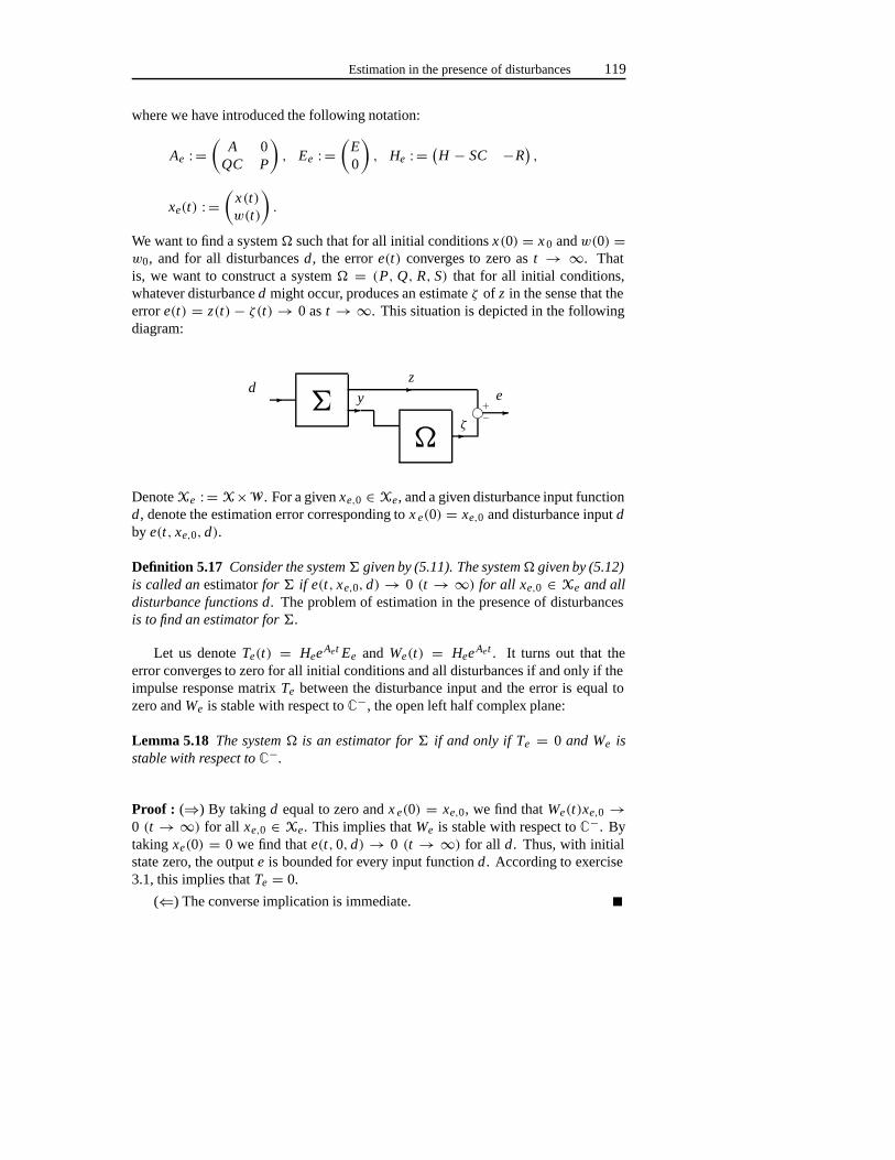
Estimation in the presence of disturbances 119
where we have introduced the following notation:
Ae : =(
A 0QC P
), Ee : =
(E0
), He : =
(H − SC −R
),
xe(t) : =(
x(t)w(t)
).
We want to find a system� such that for all initial conditionsx(0) = x 0 andw(0) =w0, and for all disturbancesd, the errore(t) converges to zero ast → ∞. Thatis, we want to construct a system� = (P, Q, R, S) that for all initial conditions,whatever disturbanced might occur, produces an estimateζ of z in the sense that theerrore(t) = z(t) − ζ(t)→ 0 ast → ∞. This situation is depicted in the followingdiagram:
� � ��
�e
� �−+
dz
y
ζ
DenoteXe : =X×W . For a givenxe,0 ∈ Xe, and a given disturbance input functiond, denote the estimation error corresponding tox e(0) = xe,0 and disturbance inputdby e(t, xe,0, d).
Definition 5.17 Consider the system� given by (5.11). The system� given by (5.12)is called an estimatorfor � if e(t, xe,0, d) → 0 (t → ∞) for all xe,0 ∈ Xe and alldisturbance functions d. The problem of estimation in the presence of disturbancesis to find an estimator for �.
Let us denoteTe(t) = HeeAet Ee and We(t) = HeeAet . It turns out that theerror converges to zero for all initial conditions and all disturbances if and only if theimpulse response matrixTe between the disturbance input and the error is equal tozero andWe is stable with respect toC−, the open left half complex plane:
Lemma 5.18 The system � is an estimator for � if and only if Te = 0 and We isstable with respect to C−.
Proof : (⇒) By takingd equal to zero andx e(0) = xe,0, we find thatWe(t)xe,0 →0 (t → ∞) for all xe,0 ∈ Xe. This implies thatWe is stable with respect toC−. Bytaking xe(0) = 0 we find thate(t,0, d) → 0 (t → ∞) for all d. Thus, with initialstate zero, the outpute is bounded for every input functiond. According to exercise3.1, this implies thatTe = 0.
(⇐) The converse implication is immediate.
120 Conditioned invariant subspaces
The problem of estimation in the presence of disturbances can thus be refor-mulated equivalently as: find a system� = (P, Q, R, S) (that is, find a finite-dimensional linear spaceW and mapsP : W → W , Q : Y → W , R : W → Z andS : Y → Z such thatTe = 0, andWe is stable with respect toC−. Of course, wemight as well pose this problem in terms of an arbitrary stability domainC g . Our firstresult gives necessary and sufficient conditions for the existence of suitable mapsP,Q andR in the case thatS is already given:
Lemma 5.19 Let Cg be a stability domain and let S : Y → Z be a map. Then thereexist a linear space W and maps P : W → W , Q : Y → W and R : W → Z suchthat the system � : = (P, Q, R, S) yields Te = 0 and We stable if and only if thereexists a (C, A)-detectability subspace S such that
im E ⊂ S ⊂ ker(H − SC).
Proof : (⇒) If Te = 0 then the system (5.13) is disturbance decoupled and hence, bytheorem 4.6, there is anAe-invariant subspaceSe such that imEe ⊂ Se ⊂ kerHe.Let Ne be the unobservable subspace of the pair(He, Ae), i.e., Ne : = 〈kerHe |Ae〉. By section 3.3,Ne is the largestAe-invariant subspace contained in kerHe andconsequently we have imEe ⊂ Ne ⊂ kerHe. Define a subspaceS of X by
S : = {x ∈ X |(
x0
)∈ Ne}.
(Here, 0 stands for the zero element ofW , the state space of the system�). It is veri-fied immediately that imE ⊂ S ⊂ ker(H − SC). We contend thatS is a detectabilitysubspace with respect to(C, A). To prove this, letx ∈ S ∩ kerC . Then(x T,0)T ∈ Ne
andCx = 0. SinceNe is invariant underAe we have(Ax0
)= Ae
(x0
)∈ Ne
and thereforeAx ∈ S. It follows that (A − λI )x ∈ S for all λ ∈ C and hencex ∈ (A − λI )−1S ∩ kerC . Conversely, if(A − λI )x ∈ S for someλ ∈ Cb andCx = 0 then
(Ae − λI )
(x0
)=
((A − λI )x
0
)∈ Ne. (5.14)
Lete be the canonical projection ontoXe/Ne. Let Ae andHe be the quotient mapsdefined bye Ae = Aee andHee = He. Then the system(He, Ae) is observable(see exercise 3.7). Also defineWe(t) : = Hee Aet . Then we haveWee = We andhence (sincee is surjective)We is stable. By theorems 3.21 and 3.23 this impliesσ( Ae) ⊂ Cg . On the other hand, since kere = Ne, it follows from (5.14) that
Aee
(x0
)= λe
(x0
).
Estimation in the presence of disturbances 121
Sinceλ ∈ Cb, the latter immediately implies that(x T,0)T ∈ Ne. It then follows thatx ∈ S and hencex ∈ S ∩ kerC . By applying theorem 5.11 we may then concludethatS is a detectability subspace.
(⇐) AssumeS is a detectability subspace with imE ⊂ S ⊂ ker(H − SC). Let : X → X/S be the canonical projection. ThenE = 0 and there exists a mapH : X/V → Z such thatH = H − SC (see section 2.4). LetG ∈ G(S) be suchthatσ(A+GC |X/S) ⊂ Cg . Define mapsP, Q andR as follows. LetW : =X/S.DefineP : = AG | X/S, Q : = −G andR : = H . We claim that with this choiceTe = 0 andWe is stable. Indeed, ifw(t) = Pw(t) + Qy(t), ζ(t) = Rw(t) + Sy(t)thene = z − ζ = H(x −w). Definee1 : = x −w. Then
e1(t) = x(t)− w(t)= Ax(t)− Pw(t) − QCx(t)
= (A + GC)x(t)− Pw(t)
= Pe1(t).
Consequently,e(t) = He1(t) = HePt e1(0). From this we see thate is independentof d soTe = 0. Also, sinceσ(P) ⊂ Cg , e is stable for all initial statesx(0) andw(0).HenceWe must be stable. This completes the proof of the lemma.
As an immediate consequence of the previous lemma we have:
Corollary 5.20 Let Cg be a stability domain and let S : Y → Z be a map. Thereexist a linear space W and maps P : W → W , Q : Y → W and R : W → Zsuch that the system � : = (P, Q, R, S) yields Te = 0 and We stable if and only ifS∗g (im E) ⊂ ker(H − SC).
The following lemma deals with the existence of a suitable mapS, representingthe direct feedthrough map of the system� to be designed:
Lemma 5.21 Let X, Y and Z be linear spaces and C : X → Y and H : X → Zbe maps. Suppose that V is a subspace of X. There exists a map S : Y → Z suchthat V ⊂ ker(H − SC) if and only if V ∩ kerC ⊂ kerH .
Proof : (⇒) This implication is immediate.
(⇐) Let V be a map such that kerV = V. Then ker(V T,CT)T ⊂ kerH sothere exists a mapL such thatL(V T,CT)T = H . PartitionL = (L1 L2) to obtainL1V + L2C = H . Define the mapS that we are looking for byS : = L 2. ThenL1V = H − SC . This implies that kerV ⊂ ker(H − SC).
By simply combining the above we obtain
Corollary 5.22 Let Cg be a stability domain. There exists a system� = (P, Q.R, S)such that Te = 0 and We is stable if and only if
S∗g (im E) ∩ kerC ⊂ kerH.
122 Conditioned invariant subspaces
In order to apply the previous result to our original estimation problem, we setCg = C−. Accordingly, denote the smallest detectability subspace containing imE ,corresponding to the stability domainC− by S∗−(im E). Then we obtain:
Corollary 5.23 There exists an estimator � for the system � if and only if
S∗−(im E) ∩ kerC ⊂ kerH.
5.4 Exercises
5.1 Using definition 5.1, give a direct proof of the fact that the intersection of twoconditioned invariant subspaces is again conditioned invariant.
5.2 Consider the system(C, A). Let T : Y → Y be an isomorphism and letG : Y → X be a linear map. Prove immediately from definition 5.2 that theclasses of(C, A)-invariant subspaces and(T C, A + GC)-invariant subspacescoincide.
5.3 Consider the system (5.1). LetS be a conditioned invariant subspace. ShowthatS is a detectability subspace if and only if(A − λI )−1S ∩ kerC ⊂ S forall λ ∈ Cb.
5.4 Consider the systemx(t) = Ax(t)+Bu(t), y(t) = Cx(t). Assume thatp = m,i.e. the dimension of the output spaceY is equal to the dimension of the inputspaceU. Let Cg be a stability domain. Assume thatC B is non-singular.
a. Show thatX = kerC ⊕ im B.
b. Let P : X → X be the projection onto kerC along imB. Assume thatσ(P A | kerC) ⊂ Cg . Show that imB is a detectability subspace.
c. Let V∗ : = V∗(kerC, A, B) andR∗ : = R∗(kerC, A, B). Show thatV∗ = kerC andR∗ = 0
d. DefineF : = −(C B)−1C A. Show thatF ∈ F(V∗).e. Show that the fixed spectrumσ(A + B F | V ∗/R∗) is equal toσ(P A |
kerC).
5.5 Consider (5.1). LetCg be a stability domain andS a subspace ofX.
a. LetS be conditioned invariant. Show thatS is inner-detectable if and onlyif
σ(A | 〈kerC | A〉 ∩ S) ⊂ Cg.
b. Assume that(C, A) is detectable. Show thatS is a detectability subspaceif and only if there existsG ∈ G(S) such thatσ(A + GC) ⊂ Cg .
5.6 Give a direct proof of theorem 5.8, based on the geometric characterization of(C, A)-invariance.
Exercises 123
5.7 Let Cg be a stability domain, and letE be a subspace ofX. Prove that
S∗g (S∗(E)) = S∗g (E).
5.8 (Observability subspaces.) Again consider the systemx(t) = Ax(t) + Bu(t),y(t) = Cx(t). A subspaceN of X is called anobservability subspace if foreach stability domainCg there exists a(Cg)-stable observer� for x/N .
a. Show that ifN is an observability subspace then for each stability domainCg there exists an observer� for x/N of the form w(t) = Pw(t) +Ry(t), ξ(t) = w(t), with σ(P) ⊂ Cg andA − P = RC (here, isthe canonical projection ontoX/N ).
b. Prove that the following statements are equivalent:
1. N is an observability subspace,2. (A − λI )−1N ∩ kerC = N ∩ kerC for all λ ∈ C,3. for each real monic polynomialp with degp = n − dimN there
existsG ∈ G(N ) such that the characteristic polynomial ofA G |X/N is equal top.
5.9 Let N be a subspace ofX. Show thatN is an observability subspace withrespect to(C, A) if and only if N ⊥ is a controllability subspace with respect to(AT,CT).
5.10 Consider the system(C, A). Let E be a subspace ofX. Let Cg be a stabilitydomain.
a. Show that there exists a smallest observability subspace,N ∗(E), contain-ing E .
b. Show thatE ⊂ S∗(E) ⊂ S∗g (E) ⊂ N ∗(E).c. DenoteN ∗ : = N ∗(E) andS∗ : = S∗(E). Show thatG(S∗) ⊂ G(N ∗)
and that for allG ∈ G(S∗) we have
N ∗ = 〈S∗ + kerC | A + GC〉.d. DetermineN ∗(0), the smallest observability subspace of(C, A).
5.11 (Computation of the smallest detectability subspace containing a given sub-space.) Consider the system(C, A). Let E be a subspace ofX and letCg be astability domain. Show that for allG ∈ G(S∗(E)) we have
S∗(E) = (Xb(A + GC) ∩ S∗(E)) ∩N ∗(E).
5.12 (Pole placement by output injection under invariance constraints.) Consider thesystem (5.1). LetS ⊂ X be a conditioned invariant subspace. In this problemwe investigate the freedom in assigning the eigenvalues ofA+GC if G : Y →X is restricted to satisfy(A + GC)S ⊂ S. Let N : = N ∗(S) be the smallestobservability subspace containingS. Furthermore, letT := S ∩ 〈kerC | A〉,the intersection ofS with the unobservable subspace of (5.1).
124 Conditioned invariant subspaces
a. Show thatG(S) ⊂ G(N ) ∩ G(T ).
b. Show that for any pair of real monic polynomials(p 1, p2), with degp1 =dimS − dimT and degp2 = n − dimN , there existG ∈ G(S) such thatχA+GC |S/T = p1 andχA+GC |X/N = p2.
c. Show that forG1,G2 ∈ G(S) we haveχA+G1C |N /S = χA+G2C |N /S, i.e.,χA+GC |N /S is fixed for allG ∈ G(S).
d. Show thatT is (A + GC)-invariant for allG : Y → X and that for allG : Y → X we haveA + GC | T = A | T .
e. Draw a lattice diagram that illustrates which parts of the spectrum ofA+GC are fixed, and which parts are free, under the restrictionG ∈ G(S).
f. Let S be an observability subspace and assume that(C, A) is observable.Show that for any real monic polynomialp of degreen such thatp =p1p2, with p1 andp2 real monic polynomials, and degp1 = dimS, thereexistsG ∈ G(S) such thatχA+GC = p.
5.5 Notes and references
Conditioned invariant subspaces were introduced by Basile and Marro in [10], andapplied to the problem of estimation in the presence of unknown disturbance inputsby the same authors in [11], see also the more recent textbook [14]. Conditionedinvariant subspaces were studied in terms of their duality properties with respect tocontrolled invariant subspaces by Morse in [129], see also the textbook by Wonham[223], page 127. The point of view of defining conditioned invariant subspaces interms of the existence of observers originates from Willems [218].
Detectability subspaces were introduced at approximately the same time by Schu-macher in [169] and Willems and Commault in [218]. The ‘hybrid’ characterizationof detectability subspaces of theorem 5.11 is due to Schumacher [169]. The definitionof observability subspace, see exercise 5.8, appeared for the first time in Willems andCommault [218].
The design of observers for systems with unknown inputs was studied by Bhat-tacharyya in [18], and by Hautus in [74]. A version of the problem was also studiedin Willems and Commault [218]. More recent material on the design of estimatorsin the presence of unknown disturbances can be found in the work of Hou, Pugh andMüller [83], and in Tsui [201]. The connection between robust observer design andthe problem of observer design with unknown inputs was studied by Bhattacharyyain [20].
Extensions toalmost conditioned invariant subspaces and, related, the design ofapproximate observers and estimators, and PID observers, can be found in the workof Willems [216].
Chapter 6
(C, A, B)-pairs and dynamicfeedback
In chapter 4 we have considered several feedback design problems that require thedesign of static state feedback control laws. Often, it is more realistic to assumethat onlypart of the state vector is available for feedback. This can be modelled byspecifying a linear function of the state vector, called the measurement output. Insteadof the entire state vector, we then only allow the use of this measurement output forfeedback. Instead of static feedback, however, we then allowdynamic feedback.
A central role in this chapter is played by the notion of(C, A, B)-pair of sub-spaces. We use this concept here to study the dynamic feedback versions of thedisturbance decoupling problem, the disturbance decoupling problem with internalstability, and, finally, the problem of external stabilization.
6.1 (C, A, B)-pairs
In this section we introduce the notion of(C, A, B)-pair of subspaces. Consider thecontrolled and observed system�:
x(t) = Ax(t)+ Bu(t),y(t) = Cx(t).
(6.1)
In section 3.9 it was explained that if we control this system using the finite-dimensi-onal linear time-invariant controller�:
w(t) = Kw(t) + Ly(t),u(t) = Mw(t) + Ny(t),
(6.2)
126 (C, A, B)-pairs and dynamic feedback
then the resulting closed loop system is described by the autonomous linear differen-tial equation(
x(t)w(t)
)=
(A + B NC B M
LC K
)(x(t)w(t)
). (6.3)
The controller (6.2) takes the observationsy as its input and generates the controlfunction u as its output. The state space of the controller is denoted byW and isassumed to be a finite-dimensional real linear space.K , L,M andN are assumed tobe linear maps fromW → W , Y → W , W → U andY → U, respectively. Thecontrol action of interconnecting the controller� with the system (6.1) is calleddy-namic feedback. The state space of the closed loop system (6.3) is called theextendedstate space and is equal to the Cartesian productX×W . The extended state space isoften denoted byXe. The system mapping of the closed loop system (6.3) is calledtheextended system mapping. Thus, the extended system mapping corresponding tothe controller� = (K , L,M, N) is equal to
Ae : =(
A + B NC B MLC K
). (6.4)
It will turn out that the control problems that are formulated and studied in this chapteressentially amount to finding linear mapsK , L,M and N such that the extendedsystem mappingAe has certain geometric properties. It is therefore important to studythe relationship between the geometric properties of the mapsA, B andC (definingthe system (6.1)) and those of the extended system maps (6.4). For describing thisrelationship it is convenient to introduce the notion of(C, A, B)-pair of subspaces.This notion is defined as follows:
Definition 6.1 Consider the system (6.1). A pair of subspaces (S,V) of X is calleda (C, A, B)-pair if S ⊂ V, S is (C, A)-invariant and V is (A, B)-invariant.
For a given subspaceVe of the extended state spaceXe = X ×W we considerthe following two subspaces of the original state spaceX:
p(Ve) : ={
x ∈ X∣∣∣ ∃ w ∈ W such that
(xw
)∈ Ve
}(6.5)
and
i(Ve) : ={
x ∈ X∣∣∣ (
x0
)∈ Ve
}. (6.6)
Note that the first subspace is theprojection of Ve onto theX-plane, whereas thesecond is theintersection of Ve with this plane. Both spaces are subspaces of theoriginal state spaceX. It turns out that, starting with a subspaceVe that is invariantunder some extended system mappingA e, the pair of subspaces obtained by takingthe intersection and projection forms a(C, A, B)-pair.
Theorem 6.2 Let Ve be a subspace of Xe that is invariant under Ae. Then
(i(Ve), p(Ve))
is a (C, A, B)-pair.
(C, A, B)-pairs 127
Proof : Obviously,i(Ve) ⊂ p(Ve). Let x ∈ i(Ve) ∩ kerC . Then we have(
Ax0
)= Ae
(x0
)∈ Ve
and henceAx ∈ i(Ve). It follows thati(Ve) is (C, A)-invariant. Next, letx ∈ p(Ve).Then there exists a vectorw ∈ W such that(x T, wT)T ∈ Ve. Consequently,(
Ax + B(NCx + Mw)LCx + Kw
)= Ae
(xw
)∈ Ve.
SinceLCx + Kw ∈ W it follows that Ax + B(NCx +Mw) ∈ p(Ve). We concludethat Ax ∈ p(Ve)+ im B. This implies thatp(Ve) is (A, B)-invariant.
The above shows thatAe-invariant subspaces of an extended state space give riseto (C, A, B)-pairs. In the sequel we also need to have some sort of converse of theo-rem 6.2, stating that if we start with a(C, A, B)-pair (S,V), there exists a controller� = (K , L,M, N) and a subspaceVe of the corresponding extended state space suchthat AeVe ⊂ Ve, p(Ve) = V andi(Ve) = S. This will be investigated now. Ourfirst step is to construct the mappingN :
Lemma 6.3 Let (S,V) be a (C, A, B)-pair. There exists a linear mapping N : Y →U such that (A + B NC)S ⊂ V.
Proof : Let q1, . . . , q j be a basis ofS ∩ kerC and extend this to a basisq1, . . . , qk ofS. SinceS ⊂ V andV is (A, B)-invariant, there existu i ∈ U andvi ∈ V such that
Aqi = vi + Bui (i = 1,2, . . . , k).
Furthermore, the vectorsCq j+1, . . . ,Cqk are linearly independent: suppose
α j+1Cq j+1+ · · · + αkCqk = 0.
Then
q : = α j+1q j+1+ · · · + αkqk ∈ S ∩ kerC
and henceq is a linear combination ofq1, . . . , q j , sayq = α1q1 + · · · + α j q j . Itfollows that
α1q1+ · · · + α j q j − α j+1q j+1− · · · − αkqk = 0.
Sinceq1, . . . , qk are linearly independent it follows thatα1 = α2 = · · · = αk = 0.This proves the assertion on the linear independence. Therefore, there exists a linearmappingN : Y → U such thatNCqi = −ui (i = j + 1, . . . , k). We then have
(A + B NC)qi = vi ∈ V (i = j + 1, . . . , k)
128 (C, A, B)-pairs and dynamic feedback
and
(A + B NC)qi = Aqi ∈ S ⊂ V (i = 1, . . . , j).
The latter follows from the facts that fori = 1, . . . , j the vectorsq i are inS ∩ kerCand thatS is (C, A)-invariant. This completes the proof of the lemma.
We now state and prove the converse of theorem 6.2 as announced above.
Theorem 6.4 Let (S,V) be a (C, A, B)-pair. Then there exists a controller (6.2) andan Ae-invariant subspace Ve of the extended state space Xe such that S = i(Ve) andV = p(Ve). Specifically, for any N : Y → U such that (A + B NC)S ⊂ V, and forany F ∈ F(V) and G ∈ G(S), the controller
w(t) = (A + B F + GC − B NC)w(t) + (B N − G)y(t),u(t) = (F − NC)w(t) + Ny(t),
(6.7)
with state space W = X, and the subspace
Ve : ={ (
x10
)+
(x2x2
)∈ Xe
∣∣∣ x1 ∈ S, x2 ∈ V}
satisfy the desired properties.
Before we give a proof of this theorem we want to make some remarks. Firstnote that the state space of the controller (6.7) is equal toX, the state space of ouroriginal system (6.1). In general, the dimension of the state space of a system iscalled itsdynamic order. Hence, the dynamic order of the controller (6.7) is equal tothe dynamic order of the system.
The controller defined by (6.7) can be interpreted as being the combination ofa state observer�, static state feedback and static output feedback. To be specific,consider the system� defined by
w(t) = (A + GC)w(t)+ Bu(t)− Gy(t),ξ(t) = w(t). (6.8)
We claim that� is a state observer for (6.1) (see definition 3.34). Indeed, if wedefinee(t) : = ξ(t) − x(t) thene(t) can be seen to satisfy the differential equatione(t) = (A + GC)e(t). Henceξ(0) = x(0) implies ξ(t) = x(t) for t � 0. If, inaddition to the equations (6.8), we consider the output equation
u(t) = (F − NC)ξ(t) + Ny(t), (6.9)
then the resulting system coincides with the controller (6.7). Thus (6.7) can be giventhe interpretation of a state observer together with a static feedback part (6.9). Thestatic feedback part generates the input valueu(t) on the basis of the state estimateξ(t) together with the measurement output valuey(t). This internal structure of thecontroller (6.7) is depicted in the following diagram:
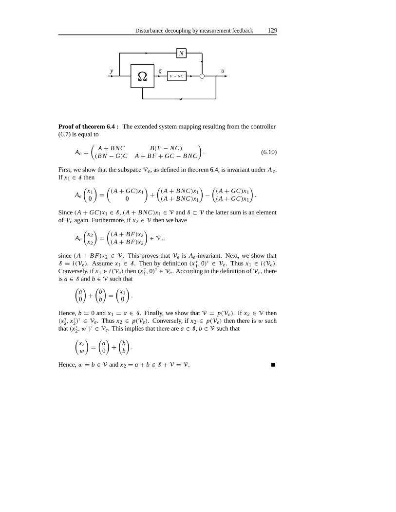
Disturbance decoupling by measurement feedback 129
� �
�
�
N
F − NC �
�
�
�
y ξ u
Proof of theorem 6.4 : The extended system mapping resulting from the controller(6.7) is equal to
Ae =(
A + B NC B(F − NC)(B N − G)C A + B F + GC − B NC
). (6.10)
First, we show that the subspaceVe, as defined in theorem 6.4, is invariant underA e.If x1 ∈ S then
Ae
(x10
)=
((A + GC)x1
0
)+
((A + B NC)x1(A + B NC)x1
)−
((A + GC)x1(A + GC)x1
).
Since(A + GC)x1 ∈ S, (A + B NC)x1 ∈ V andS ⊂ V the latter sum is an elementof Ve again. Furthermore, ifx2 ∈ V then we have
Ae
(x2x2
)=
((A + B F)x2(A + B F)x2
)∈ Ve,
since(A + B F)x2 ∈ V. This proves thatVe is Ae-invariant. Next, we show thatS = i(Ve). Assumex1 ∈ S. Then by definition(x T
1,0)T ∈ Ve. Thusx1 ∈ i(Ve).
Conversely, ifx1 ∈ i(Ve) then(x T
1,0)T ∈ Ve. According to the definition ofVe, there
is a ∈ S andb ∈ V such that(a0
)+
(bb
)=
(x10
).
Hence,b = 0 andx1 = a ∈ S. Finally, we show thatV = p(Ve). If x2 ∈ V then(x T
2, x T
2)T ∈ Ve. Thusx2 ∈ p(Ve). Conversely, ifx2 ∈ p(Ve) then there isw such
that(x T
2, wT)T ∈ Ve. This implies that there area ∈ S, b ∈ V such that(
x2w
)=
(a0
)+
(bb
).
Hence,w = b ∈ V andx2 = a + b ∈ S + V = V.
130 (C, A, B)-pairs and dynamic feedback
6.2 Disturbance decoupling by measurement feedback
Consider the control system
x(t) = Ax(t)+ Bu(t)+ Ed(t),y(t) = Cx(t),z(t) = H x(t).
(6.11)
Again,d represents a disturbance input. The functions d that can occur are assumedto be elements of a given function space. The variablez represents a to-be-controlledoutput. We want to control the system such that in the closed loop system the outputzdoes not depend on the disturbance inputd. In section 4.2 we considered this problemfor the case that the control inputu(t) is allowed to depend on the current statex(t)via some static state feedback control lawu(t) = Fx(t). Implicitly, this assumes thatthe entire state vectorx can be used for control purposes, at any time instantt � 0.Often, it is more realistic to assume that we have access only topart of the state vectorx . This can be formalized by including the additional output equationy(t) = Cx(t)in the set of equations of the control system (withC a linear mapping from the statespaceX into some finite-dimensional linear spaceY), and to require the feedbackmechanism that generatesu to be driven by the outputy (themeasurement output).Here, we will allow these feedback mechanisms to be given by controllers� of theform (6.2). If the control system (6.11) and the controller (6.2) are interconnected,then the resulting closed loop system is described by the equations(
x(t)w(t)
)=
(A + B NC B M
LC K
)(x(t)w(t)
)+
(E0
)d(t),
z(t) = (H 0
) (x(t)w(t)
).
(6.12)
In addition to the compact notation (6.4) for the system mappingA e of (6.12), weintroduce
Ee : =(
E0
)and He : =
(H 0
).
For a given controller� = (K , L,M, N), the corresponding closed loop impulseresponse matrix betweend andz is denoted byT� and is equal to
T�(t) : = HeeAet Ee.
The corresponding transfer functionHe(I s − Ae)−1e Ee is denoted byG�(s). The
problem of disturbance decoupling by measurement feedback is to find a controller� such that the closed loop system (6.12) is disturbance decoupled (see section 4.2).We stress that this amounts to identifying a suitable finite-dimensional linear spaceW (the state space of the controller), together with four mapsK , L,M andN :
Definition 6.5 Consider the system (6.11). The problem of disturbance decouplingby measurement feedback, DDPM, is to find a controller � = (K , L,M, N) suchthat T� = 0 (or, equivalently, such that G� = 0).

Disturbance decoupling by measurement feedback 131
Our aim is now to establish necessary and sufficient conditions for the existenceof a controller that makes the closed loop system disturbance decoupled. We wantthese conditions to be entirely in terms of the original control system (6.11), that is,in terms only of the mapsA, B,C, E and H . It turns out that the previous sectionprovides most of the ingredients to establish such conditions:
Theorem 6.6 There exists a controller � such that T� = 0 if and only if there existsa (C, A, B)-pair (S,V) such that im E ⊂ S ⊂ V ⊂ kerH .
Proof : (⇒) Assume that (6.12) is disturbance decoupled. According to theorem 4.6there exists anAe-invariant subspaceVe such that imEe ⊂ Ve ⊂ kerHe. DefineS : = i(Ve) andV : = p(Ve). According to theorem 6.2,(S,V) is a(C, A, B)-pair.Let x ∈ im E . Then(x T,0)T ∈ im Ee ⊂ Ve, sox ∈ i(Ve) = S. Let x ∈ V = p(Ve).Then there existsw ∈ W (the state space of the controller�) such that(x T, wT)T ∈Ve ⊂ kerHe. HenceH x = He(x T, wT)T = 0, soV ⊂ kerH .
(⇐) Conversely, let(S,V) be a(C, A, B)-pair between imE and kerH . Accord-ing to theorem 6.4 there exists a controller� and anA e-invariant subspaceVe of theextended state space such thatS = i(Ve) andV = p(Ve). We claim that
im Ee ⊂ Ve ⊂ kerHe.
Indeed,(x T, wT)T ∈ im Ee impliesw = 0 andx ∈ im E ⊂ S. Consequently(xw
)=
(x0
)∈ Ve.
Furthermore,(x T, wT)T ∈ Ve implies thatx ∈ V ⊂ kerH . HenceHe(x T, wT)T =H x = 0. This proves the claim. It then follows from theorem 4.6 that the closed loopsystem (6.12) is disturbance decoupled.
Let S∗(im E) be the smallest(C, A)-invariant subspace containing imE (see the-orem 5.7) and letV∗(kerH ) be the largest(A, B)-invariant subspace contained inkerH (see theorem 4.5). If the conditionS ∗(im E) ⊂ V∗(kerH ) holds then ob-viously (S∗(im E),V∗(kerH )) is a (C, A, B)-pair between imE and kerH . Con-versely, if (S,V) is a (C, A, B)-pair such that imE ⊂ S andV ⊂ kerH then wemust haveS∗(im E) ⊂ S andV ⊂ V∗(kerH ). Thus, we obtain the followingcorollary:
Corollary 6.7 There exists a controller � such that T� = 0 if and only if
S∗(im E) ⊂ V∗(kerH ).
The condition of corollary 6.7 can be checked computationally by means of the in-variant subspace algorithm, ISA, described in section 4.3 (see theorem 4.10) and theconditioned invariant subspace algorithm, CISA, described in section 5.1 (see theo-rem 5.8). If the subspace inclusion of corollary 6.7 holds then a procedure to calculate
132 (C, A, B)-pairs and dynamic feedback
an actual controller� can immediately be obtained from theorem 6.4. First, we cal-culate a mappingF : X → U such thatA FV∗ ⊂ V∗, a mappingG : Y → X suchthat AGS∗ ⊂ S∗ and a mappingN : Y → U such that(A + B NC)S∗ ⊂ V∗. Nextwe putK : = A+ B F+GC− B NC, L : = B N −G andM : = F− NC . The con-troller � defined byw(t) = Kw(t) + Ly(t), u(t) = Mw(t) + Ny(t) then achievesthe desired disturbance decoupling. The state space of� is equal toW = X, so itsdynamic order is equal to the dynamic order of the underlying control system.
6.3 (C, A, B)-pairs and internal stability
In section 6.1 it was shown how a(C, A, B)-pair leads to an extended system map-ping and an invariant subspace of the extended state space such that certain propertieshold. In this section we study the connection between the spectrum of the extendedsystem mapping and the stabilizability and detectability properties of the underlying(C, A, B)-pair.
Recall from theorem 6.2 that if we have an extended system mappingA e of theform (6.4) working on some extended state spaceX e, and ifVe is a subspace ofXe
that is Ae-invariant, then(i(Ve), p(Ve)) constitutes a(C, A, B)-pair. The followingresult is more specific:
Theorem 6.8 Let Ve be an Ae-invariant subspace of Xe. Then we have:
(i) if Ve is inner-stable, then i(Ve) is inner-detectable and p(Ve) is inner-stabili-zable,
(ii) if Ve is outer-stable, then i(Ve) is outer-detectable and p(Ve) is outer-stabili-zable.
Proof : (i) SinceVe is inner-stable, it follows from theorem 2.17 that
(λI − Ae)Ve = Ve
for all λ ∈ Cb. We first show thatp(Ve) satisfies the condition (ii) of theorem 4.22.By theorem 6.2,p(Ve) is controlled invariant so for allλ ∈ C we have
(λI − A)p(Ve)+ im B ⊂ p(Ve)+ im B.
Let λ ∈ Cb and letx ∈ p(Ve). We have to show thatx can be written as(λI −A)x + Bu, for somex ∈ p(Ve) andu ∈ U. Sincex ∈ p(Ve), there existsw ∈ Wsuch thatxe : = (x T, wT)T ∈ Ve. There existsxe ∈ Ve, sayxe = (x T, wT)T, such that(λI − Ae)xe = xe. This however implies
(λI − A − B NC)x − B Mw = x .
If we defineu : = −(NCx + Mw) then this yields the desired representation ofx(note thatx ∈ p(Ve)). We conclude thatp(Ve) is a stabilizability subspace. Next, we
(C, A, B)-pairs and internal stability 133
show thati(Ve) is inner-detectable. It was already shown thati(Ve) is conditionedinvariant. Thus, we have to show that
σ(A | i(Ve) ∩ 〈kerC | A〉) ⊂ Cg
(see exercise 5.5). Letλ andx be such thatAx = λx and such thatx ∈ 〈kerC | A〉∩ i(Ve), x = 0. SinceCx = 0 we obtain
Ae
(x0
)=
(Ax0
)= λ
(x0
).
Using the fact thatx ∈ i(Ve) we have(x T,0)T ∈ Ve. Henceλ ∈ σ(Ae | Ve) ⊂ Cg .
(ii) If Ve is outer-stable thenV⊥e is inner-stable with respect toATe . Since
ATe =
(AT + CT N T BT CT LT
MT BT K T
)
we can conclude from (i) thati(V⊥e ) is inner-detectable with respect to(B T, AT) and
that p(V⊥e ) is inner-stabilizable with respect to(AT,CT). By exercise 6.1, we havei(V⊥e ) = p(Ve)
⊥ and p(V⊥e ) = i(Ve)⊥. Thus, we conclude thatp(Ve) is outer-
stabilizable and thati(Ve) is a detectability subspace (see theorem 5.13).
Our next result is, in a sense, the converse of theorem 6.8. As we already sawin section 6.1, if(S,V) is a (C, A, B)-pair then we can construct a controller�and anAe-invariant subspaceVe of the associated extended state spaceXe such thati(Ve) = S and p(Ve) = V. The following theorem shows how the spectrum ofA e
depends on the spectra ofA + B F and A + GC , if the linear mapsF and G arechosen fromF(V) andG(S), respectively.
Theorem 6.9 Let (S,V) be a (C, A, B)-pair. Assume that F ∈ F(V) and G ∈G(S). Then there exists a controller � and an Ae-invariant subspace Ve of the ex-tended state space Xe such that i(Ve) = S, p(Ve) = V and
σ(Ae | Ve) = σ(AF | V) ∪ σ(AG | S), (6.13)
σ(Ae | Xe/Ve) = σ(AF | X/V) ∪ σ(AG | X/S). (6.14)
Specifically, if N : Y → U is a linear mapping such that (A + B NC)S ⊂ V thenthe controller
w(t) = (A + B F + GC − B NC)w(t) + (B N − G)y(t),u(t) = (F − NC)w(t) + Ny(t),
(6.15)
with state space W = X, and the subspace
Ve : ={ (
x10
)+
(x2x2
) ∣∣∣ x1 ∈ S, x2 ∈ V}
(6.16)
satisfy the desired properties.
134 (C, A, B)-pairs and dynamic feedback
Proof : The facts that the controller (6.15) and the subspaceV e given by (6.16) havethe properties thati(Ve) = S, p(Ve) = V andVe is Ae-invariant were alreadyproven in theorem 6.4. It remains to show (6.13) and (6.14). We first prove (6.13).Let xe ∈ Ve be an eigenvector ofAe with eigenvalueλ. Write
xe =(
x1+ x2x2
)
with x1 ∈ S andx2 ∈ V. Using (6.10), the expressionAexe = λxe becomes
(A + B NC)x1 + (A + B F)x2 = λ(x1+ x2), (6.17)
(B NC − GC)x1+ (A + B F)x2 = λx2. (6.18)
Subtracting (6.18) from (6.17) yields
(A + GC)x1 = λx1.
First assumex1 = 0. Then we may concludeλ ∈ σ(AG | S). If, on the other hand,x1 = 0 then (6.18) becomes
(A + B F)x2 = λx2.
Since in that casex2 = 0 (xe = 0 !) the latter implies thatλ ∈ σ(AG | V). We nowprove the converse inclusion in (6.13). Assume 0= x 2 ∈ V such thatAF x2 = λx2.Define xe : = (x T
2, x T
2)T. Thenxe ∈ Ve and Aexe = λxe. Thusλ ∈ σ(Ae | Ve).
Next, assume that 0= x1 ∈ S with AG x1 = λx1. Since(x T
1,0)T ∈ Ve, sinceVe is
Ae- invariant and since
Ae
(x10
)=
((A + B NC)x1(B NC − GC)x1
),
the vectorx1 : = (B NC − GC)x1 lies in V. Now, we may assume thatλ ∈ σ(A F |V). In that case the mapping(λI − A F ) | V is invertible and the equation
x1+ (λI − AF )x2 = 0
has a (unique) solutionx2 ∈ V. Define then
xe : =(
x1+ x2x2
)∈ Ve.
It can then be verified that
Aexe =(
AG x1+ x1+ (λI − AF )x2+ λx2x1+ (λI − AF )x2+ λx2
)= λ
(x1+ x2
x2
)= λxe.
Sincex1 = 0, alsoxe = 0. Henceλ ∈ σ(Ae | Ve). Thus we have proven (6.13). Wenow prove (6.14). We do this by dualization of the first part of this theorem. Define asubspace of the extended state space by
Ve : ={ (
x10
)+
(x2−x2
) ∣∣∣ x1 ∈ V⊥, x2 ∈ S⊥}.
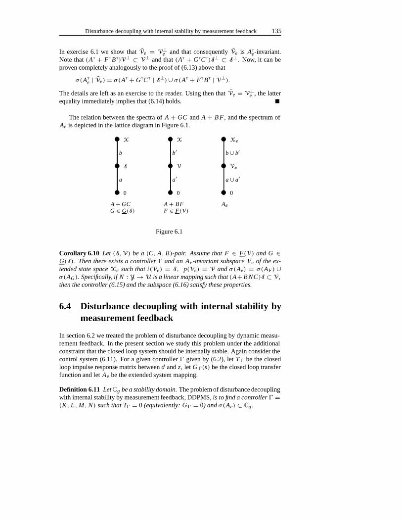
Disturbance decoupling with internal stability by measurement feedback135
In exercise 6.1 we show thatVe = V⊥e and that consequentlyVe is ATe-invariant.
Note that(AT + FT BT)V⊥ ⊂ V⊥ and that(AT + GTCT)S⊥ ⊂ S⊥. Now, it can beproven completely analogously to the proof of (6.13) above that
σ(ATe | Ve) = σ(AT + GTCT | S⊥) ∪ σ(AT + FT BT | V⊥).
The details are left as an exercise to the reader. Using then thatVe = V⊥e , the latterequality immediately implies that (6.14) holds.
The relation between the spectra ofA + GC and A + B F , and the spectrum ofAe is depicted in the lattice diagram in Figure 6.1.
S
a
F ∈ F(V)G ∈ G(S)Ae
0
a ∪ a′Ve
b ∪ b′Xe
A + B F
0
X
b
0
A + GC
X
b′
V
a′
Figure 6.1
Corollary 6.10 Let (S,V) be a (C, A, B)-pair. Assume that F ∈ F(V) and G ∈G(S). Then there exists a controller � and an Ae-invariant subspace Ve of the ex-tended state space Xe such that i(Ve) = S, p(Ve) = V and σ(Ae) = σ(AF ) ∪σ(AG). Specifically, if N : Y → U is a linear mapping such that (A+B NC)S ⊂ V,then the controller (6.15) and the subspace (6.16) satisfy these properties.
6.4 Disturbance decoupling with internal stability bymeasurement feedback
In section 6.2 we treated the problem of disturbance decoupling by dynamic measu-rement feedback. In the present section we study this problem under the additionalconstraint that the closed loop system should be internally stable. Again consider thecontrol system (6.11). For a given controller� given by (6.2), letT� be the closedloop impulse response matrix betweend andz, let G �(s) be the closed loop transferfunction and letAe be the extended system mapping.
Definition 6.11 Let Cg be a stability domain. The problem of disturbance decouplingwith internal stability by measurement feedback, DDPMS, is to find a controller � =(K , L,M, N) such that T� = 0 (equivalently: G� = 0) and σ(Ae) ⊂ Cg.
136 (C, A, B)-pairs and dynamic feedback
In order to establish necessary and sufficient conditions for the existence of acontroller that makes the closed loop system disturbance decoupled and internallystable, we use the following lemma:
Lemma 6.12 Let (S,V) be a (C, A, B)-pair, where S is a detectability subspaceand V is a stabilizability subspace. Assume that (C, A) is detectable and (A, B)is stabilizable. Then there exists a controller � such that σ(Ae) ⊂ Cg and an Ae-invariant subspace Ve of the extended state space Xe such that i(Ve) = S andp(Ve) = V.
Proof : According to theorem 4.32 there existsF ∈ F(V) such thatσ(A F ) ⊂ Cg . Bydualizing theorem 4.32, we find that there existsG ∈ G(S) such thatσ(A G) ⊂ Cg .Finally, there exists a linear mappingN : Y → U such that(A + B NC)S ⊂ V. Byapplying corollary 6.10 we then find a controller� with the desired properties.
Theorem 6.13 There exists a controller � such that T� = 0 and σ(Ae) ⊂ Cg if andonly if there exist a detectability subspace S and a stabilizability subspace V suchthat
im E ⊂ S ⊂ V ⊂ kerH,
(C, A) is detectable, and (A, B) is stabilizable.
Proof : (⇒) If T� = 0 then the closed loop system (6.12) is disturbance decoupled.By theorem 4.6, there is anAe-invariant subspaceVe of the extended state spaceXe
such that imEe ⊂ Ve ⊂ kerHe. Since, furthermore,σ(Ae) ⊂ Cg , the subspaceVe must be inner-stable and outer-stable. According to theorem 6.8, this impliesthatS : = i(Ve) is a detectability subspace and thatV : = p(Ve) is a stabilizabilitysubspace. The claim that imE ⊂ S ⊂ V ⊂ kerH was already proven in theorem6.6. The facts that(C, A) is detectable and(A, B) is stabilizable follow from theorem3.40 (note that� is a stabilizing controller).
(⇐) By lemma 6.12, there is a controller� such thatσ(A e) ⊂ Cg and anAe-invariant subspaceVe such thati(Ve) = S and p(Ve) = V. We showed in theorem6.6 that the latter implies that imEe ⊂ Ve ⊂ kerHe. According to theorem 4.6 wemust therefore have that the closed loop system (6.12) is disturbance decoupled.
The previous result immediately yields the following corollary which providesconditions that can be checked computationally:
Corollary 6.14 There exists a controller � such that T� = 0 and σ(Ae) ⊂ Cg if andonly if
S∗g (im E) ⊂ V∗g (kerH ),
(C, A) is detectable, and (A, B) is stabilizable.
Pairs of(C, A, B)-pairs 137
Proof : The proof of this is left as an exercise to the reader.
If (C, A) is detectable,(A, B) is stabilizable, and the subspace inclusion of corol-lary 6.14 holds, then a suitable controller can be calculated as follows. First, take amappingF : X → U such thatA FV∗g ⊂ V∗g andσ(AF ) ⊂ Cg (see theorem 4.32).Find a mappingG : Y → X such thatAGS∗g ⊂ S∗g andσ(AG) ⊂ Cg (dual oftheorem 4.32). Next, letN : Y → U be such that(A + B NC)S ∗g ⊂ V∗g . PutK : = A + B F + GC − B NC , L : = B N − G and M : = F − NC . Then thecontroller� = (K , L,M, N) with state spaceW = X will achieve disturbancedecoupling and internal stability.
6.5 Pairs of(C, A, B)-pairs
In the previous sections we have seen how(C, A, B)-pairs can be used to constructcontrollers. We showed that a(C, A, B)-pair between imE and kerH immediatelygives rise to a controller that achieves disturbance decoupling. In the present sectionwe will rather work withpairs of (C, A, B)-pairs. These will be applied to extendthe results of section 4.8 on the problem of external stabilization from the static statefeedback case to the case of dynamic measurement feedback.
First consider the situation that we have two(A, B)-invariant subspacesV1 andV2 such thatV1 ⊂ V2. We may then ask ourselves the question: does there existsa single linear mappingF : X → U such that bothV1 andV2 are invariant underA + B F? The answer is yes:
Lemma 6.15 Let V1 ⊂ V2 be (A, B)-invariant subspaces. Then there exists a linearmapping F : X→ U such that (A + B F)Vi ⊂ Vi (i = 1,2).
Proof : Let F1 ∈ F(V1) and F2 ∈ F(V2). Choose a basis forX as follows. Firstchoose a basisq1, . . . , qk for V1. Extend this to a basisq1, . . . , ql for V2 and subse-quently to a basisq1, . . . , qn for X. Let F be a linear mappingX → U such thatFqi = F1qi (i = 1, . . . , k) andFqi = F2qi (i = k + 1, . . . , l). It is easily verifiedthat F ∈ F(V1) ∩ F(V2).
Of course, this result can immediately be dualized to obtain the correspondingresult for conditioned invariant subspaces:
Lemma 6.16 Let S1 ⊂ S2 be (C, A)-invariant subspaces. There exists a linear map-ping G : Y → X such that (A + GC)Si ⊂ Si (i = 1,2).
Proof : The proof of this lemma is left as an exercise to the reader (use theorem 5.6).
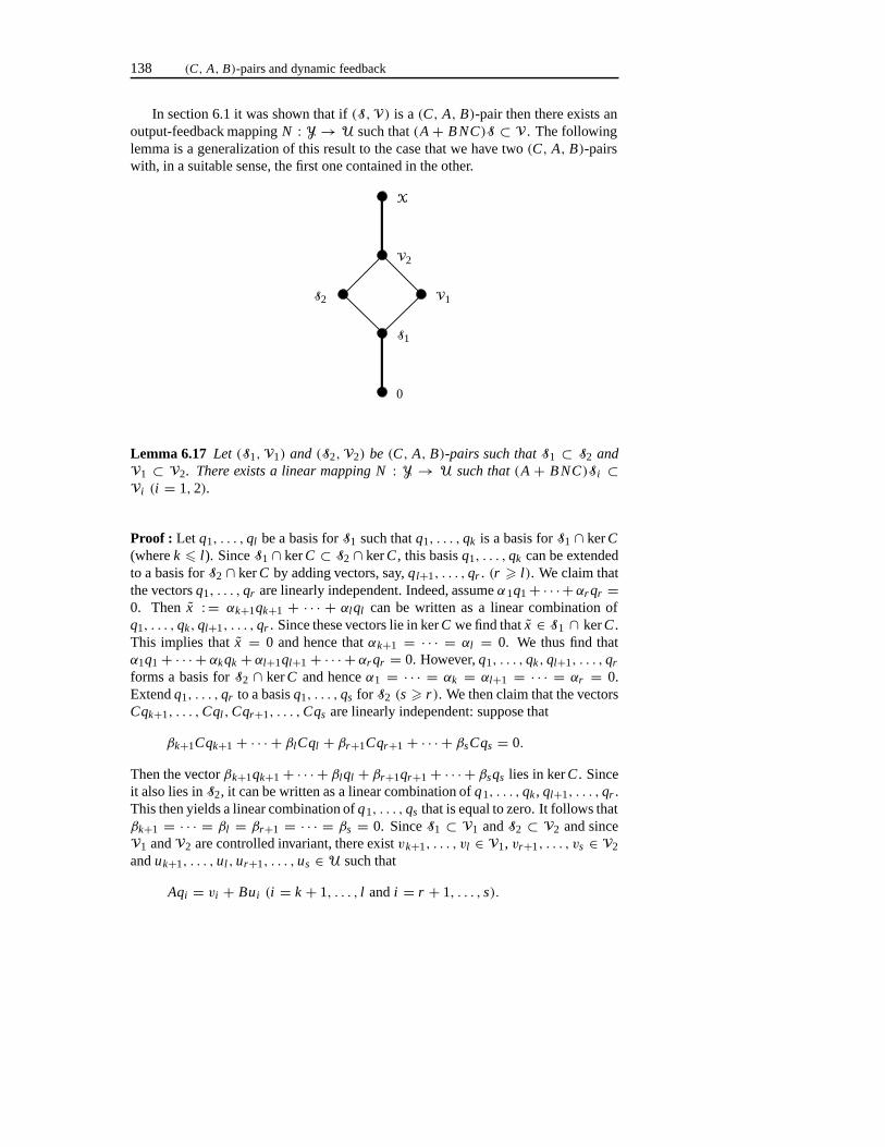
138 (C, A, B)-pairs and dynamic feedback
In section 6.1 it was shown that if(S,V) is a(C, A, B)-pair then there exists anoutput-feedback mappingN : Y → U such that(A + B NC)S ⊂ V. The followinglemma is a generalization of this result to the case that we have two(C, A, B)-pairswith, in a suitable sense, the first one contained in the other.
V1
X
S2
0
S1
V2
Lemma 6.17 Let (S1,V1) and (S2,V2) be (C, A, B)-pairs such that S1 ⊂ S2 andV1 ⊂ V2. There exists a linear mapping N : Y → U such that (A + B NC)Si ⊂Vi (i = 1,2).
Proof : Let q1, . . . , ql be a basis forS1 such thatq1, . . . , qk is a basis forS1 ∩ kerC(wherek � l). SinceS1 ∩ kerC ⊂ S2 ∩ kerC , this basisq1, . . . , qk can be extendedto a basis forS2 ∩ kerC by adding vectors, say,ql+1, . . . , qr . (r � l). We claim thatthe vectorsq1, . . . , qr are linearly independent. Indeed, assumeα1q1+ · · ·+ αr qr =0. Then x : = αk+1qk+1 + · · · + αlql can be written as a linear combination ofq1, . . . , qk, ql+1, . . . , qr . Since these vectors lie in kerC we find thatx ∈ S1 ∩ kerC .This implies thatx = 0 and hence thatαk+1 = · · · = αl = 0. We thus find thatα1q1+ · · · + αkqk + αl+1ql+1+ · · · + αr qr = 0. However,q1, . . . , qk, ql+1, . . . , qr
forms a basis forS2 ∩ kerC and henceα1 = · · · = αk = αl+1 = · · · = αr = 0.Extendq1, . . . , qr to a basisq1, . . . , qs for S2 (s � r). We then claim that the vectorsCqk+1, . . . ,Cql ,Cqr+1, . . . ,Cqs are linearly independent: suppose that
βk+1Cqk+1 + · · · + βlCql + βr+1Cqr+1 + · · · + βsCqs = 0.
Then the vectorβk+1qk+1+ · · · + βlql + βr+1qr+1+ · · · + βsqs lies in kerC . Sinceit also lies inS2, it can be written as a linear combination ofq1, . . . , qk , ql+1, . . . , qr .This then yields a linear combination ofq1, . . . , qs that is equal to zero. It follows thatβk+1 = · · · = βl = βr+1 = · · · = βs = 0. SinceS1 ⊂ V1 andS2 ⊂ V2 and sinceV1 andV2 are controlled invariant, there existvk+1, . . . , vl ∈ V1, vr+1, . . . , vs ∈ V2anduk+1, . . . , ul , ur+1, . . . , us ∈ U such that
Aqi = vi + Bui (i = k + 1, . . . , l andi = r + 1, . . . , s).
Pairs of(C, A, B)-pairs 139
SinceCqk+1, . . . ,Cql ,Cqr+1, . . . ,Cqs are linearly independent, there exists a linearmappingN : Y → U such thatNCqi = −ui (i = k+1, . . . , l andi = r+1, . . . , s).We then have
(A + B NC)qi = Aqi ∈ S1 ⊂ V1 (i = 1, . . . , k),
(A + B NC)qi = vi ∈ V1 (i = k + 1, . . . , l),
which implies(A + B NC)S1 ⊂ V1. In the same way we find that
(A + B NC)qi = Aqi ∈ S2 ⊂ V2 (i = 1, . . . , r),
(A + B NC)qi = vi ∈ V2(i = r + 1, . . . , s),
which implies that(A + B NC)S2 ⊂ V2.
By combining the previous three lemmas with theorem 6.4 and corollary 6.10, wearrive at the following theorem:
Theorem 6.18 Let (S1,V1) and (S2,V2) be (C, A, B)-pairs such that S1 ⊂ S2 andV1 ⊂ V2. Let F ∈ F(V1) ∩ F(V2), and let G ∈ G(S1) ∩ G(S2). Then there exists acontroller � and Ae-invariant subspaces Ve,1 ⊂ Ve,2 of the extended state space Xe
such that
i(Ve,1) = S1, p(Ve,1) = V1, (6.19)
i(Ve,2) = S2, p(Ve,2) = V2, (6.20)
σ(Ae) = σ(AF ) ∪ σ(AG), (6.21)
σ(Ae | Ve,2/Ve,1) = σ(AF | V2/V1) ∪ σ(AG | S2/S1). (6.22)
Specifically, for any linear mapping N : Y → U such that (A+ B NC)S i ⊂ Vi (i =1,2) the controller � given by
w(t) = (A + B F + GC − B NC)w(t) + (B N − G)y(t),u(t) = (F − NC)w(t) + Ny(t)
(6.23)
with state space W = X, and the subspaces
Ve,i : ={ (
x10
)+
(x2x2
)∈ Xe
∣∣∣ x1 ∈ Si , x2 ∈ Vi
}(i = 1,2) (6.24)
satisfy these desired properties.
Proof : The claim that the controller� given by (6.23) yields an extended systemmappingAe under which the subspaces (6.24) are invariant follows from theorem 6.4.Also (6.19) and (6.20) follow from theorem 6.4. Property (6.21) is a consequence ofcorollary 6.10. The fact thatVe,1 ⊂ Ve,2 follows from the definition. It remainsto prove (6.22). Let : Ve,2 → Ve,2/Ve,1 be the canonical projection. Denotethe mappingAe | Ve,2/Ve,1 by Ae0. Let λ ∈ σ(Ae0) and letxe be an associated
140 (C, A, B)-pairs and dynamic feedback
eigenvector(xe ∈ Ve,2). Since ker = Ve,1 we havexe ∈ Ve,1. By the fact thatAe0 = Ae we haveAexe = λxe. Hence there exists a vectorxe ∈ Ve,1 suchthat Aexe = λxe + xe. From the definition ofVe,1 andVe,2 we find that there arex1 ∈ S1, x2 ∈ V1, x1 ∈ S2 andx2 ∈ V2 such that
xe =(
x1+ x2x2
)and xe =
(x1+ x2
x2
).
Using the representation (6.10) forA e this yields
(A + B NC)(x1 + x2)+ (B F − B NC)x2 = λ(x1+ x2)+ x1+ x2, (6.25)
(B NC − GC)(x1+ x2)+ (A + B F + GC − B NC)x2 = λx2 + x2. (6.26)
This, in turn, yields
(A + B NC)x1 + (A + B F)x2 = λ(x1+ x2)+ x1+ x2, (6.27)
(B NC − GC)x1+ (A + B F)x2 = λx2+ x2. (6.28)
By subtracting (6.28) from (6.27) we obtain
(A + GC)x1 = λx1+ x1. (6.29)
Let1 : V2 → V2/V1 and2 : S2 → S2/S1 be the canonical projections. DenoteAF | V2/V1 by A1 and AG | S2/S1 by A2. We now distinguish two cases, the casethatx1 ∈ S1 and the case thatx1 ∈ S1. First assume thatx1 ∈ S1. Then2x1 = 0.Sincex1 ∈ S1 it follows from (6.29) that
A22x1 = 2AG x1 = λ2x1.
Hence,2x1 is an eigenvector ofA2 with eigenvalueλ soλ ∈ σ(AG | S2/S1). Next,assumex1 ∈ S1. Sincex1, x2 ∈ V1 and(A + B NC)x1 ∈ V1 it then follows from(6.27) that
A11x2 = 1AF x2 = λ1x2.
We claim that1x2 = 0. Indeed,x2 ∈ V1 would, together withx1 ∈ S1, implythat xe ∈ V1,e. This is a contradiction. Hence,1x2 is an eigenvector ofA1 witheigenvalueλ soλ ∈ σ(AF | V2/V1). We have now proven that in (6.22) we haveinclusion from the left to the right.
To prove the converse inclusion, letλ ∈ σ(A1). There isx2 ∈ V2, x2 ∈ V1 suchthat
A11x2 = λ1x2.
Consequently, there is a vectorx2 ∈ V1 such that
AF x2 = λx2+ x2.
External stabilization by measurement feedback 141
Define
xe : =(
x2x2
)and xe : =
(x2x2
).
Thenx2 ∈ Ve,2 andxe ∈ Ve,1. It is straightforward to verify that
Aexe = λxe + xe
and henceAe0xe = Aexe = λxe. Sincex2 ∈ V1 we must havexe = 0 andhencexe is an eigenvector ofAe0 with eigenvalueλ. We conclude thatλ ∈ σ(Ae |Ve,2/Ve,1). To prove the fact that also the spectrum ofA G | S2/S1 is contained inthe spectrum ofAe | Ve,2/Ve,1, assume thatλ ∈ σ(A2). There isx1 ∈ S2, x1 ∈ S1such that
A22x1 = λ2x1.
Consequently, there exists a vectorx1 ∈ S1 such that
AG x1 = λx1+ x1.
The vector(
x10
)lies inVe,2 and since this subspace isAe-invariant we have
Ae
(x10
)=
((A + B NC)x1(B NC − GC)x1
)∈ Ve,2.
This immediately implies that(B NC − GC)x1 ∈ V2. Now, assume thatλ ∈ σ(AF |V2/V1). Then(A1− λI )−1 exists. Letx2 ∈ V2 be such that
(A1− λI )−11(B NC − GC)x1 = −1x2.
The latter implies that
1(B NC − GC)x1 = −1(AF − λI )x2
and therefore
x2 : = (B NC − GC)x1+ (AF − λI )x2 ∈ V1.
Define nowxe ∈ V2,e andxe ∈ V1,e by
xe : =(
x1+ x2x2
), xe : =
(x2x2
).
Sincex1 ∈ S1 we must havexe ∈ V1,e. Hencexe = 0. It is now easily verified that
Aexe =((A + B NC)x1 + AF x1(B NC − GC)x1+ AF x2
)=
(AG x1+ λx2+ x2
λx2+ x2
)= λxe + xe.
From this we obtain that
Ae0xe = Aexe = λxe,
and we conclude thatλ ∈ σ(Ae0). This completes the proof of the theorem.
The relation between the spectra ofA + GC and A + B F , and the spectrum ofAe is depicted in the lattice diagram (6.2).
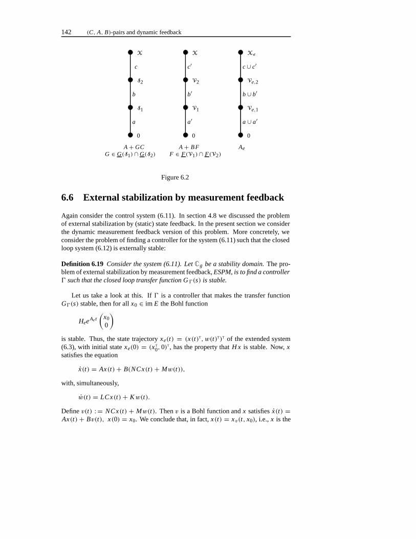
142 (C, A, B)-pairs and dynamic feedback
0
A + GCG ∈ G(S1) ∩ G(S2) F ∈ F(V1) ∩ F(V2)
Ve,1
Ve,2
V1
V2S2
S1
c ∪ c′c′c
XeXX
Ae
0
b
a
b′
a′
0
A + B F
b ∪ b′
a ∪ a′
Figure 6.2
6.6 External stabilization by measurement feedback
Again consider the control system (6.11). In section 4.8 we discussed the problemof external stabilization by (static) state feedback. In the present section we considerthe dynamic measurement feedback version of this problem. More concretely, weconsider the problem of finding a controller for the system (6.11) such that the closedloop system (6.12) is externally stable:
Definition 6.19 Consider the system (6.11). Let Cg be a stability domain. The pro-blem of external stabilization by measurement feedback, ESPM, is to find a controller� such that the closed loop transfer function G�(s) is stable.
Let us take a look at this. If� is a controller that makes the transfer functionG�(s) stable, then for allx0 ∈ im E the Bohl function
HeeAet(
x00
)
is stable. Thus, the state trajectoryxe(t) = (x(t)T, w(t)T)T of the extended system(6.3), with initial statexe(0) = (x T
0,0)T, has the property thatH x is stable. Now,x
satisfies the equation
x(t) = Ax(t)+ B(NCx(t) + Mw(t)),
with, simultaneously,
w(t) = LCx(t)+ Kw(t).
Definev(t) : = NCx(t) + Mw(t). Thenv is a Bohl function andx satisfiesx(t) =Ax(t)+ Bv(t), x(0) = x0. We conclude that, in fact,x(t) = xv(t, x0), i.e.,x is the

External stabilization by measurement feedback 143
state trajectory of the system(A, B) resulting from the initial statex(0) = x 0 and thecontrol inputv. SinceH x is stable, this immediately implies thatx 0 is an elementof the subspaceWg(kerH ) defined by (4.28). Since this holds for anyx 0 ∈ im E ,after applying theorem 4.37 we obtain as a necessary condition for the existence ofan externally stabilizing controller� that
im E ⊂ V∗(kerH )+Xstab. (6.30)
We can say even more. For, if� is such thatG�(s) is stable then also the transposedtransfer matrix
GT�(s) = ET
e(I s − ATe)−1H T
e
is stable. Since
ATe =
(AT + CT N T BT CT LT
MT BT K T
), H T
e =(
H T
0
),
ETe =
(ET 0
),
this implies that the controller� = (K T,MT, LT, N T) achieves external stability forthe dual control system
x(t) = ATx(t)+ CTu(t)+ H Td(t),y(t) = BTx(t),z(t) = ETx(t).
(6.31)
This immediately implies that
im H T ⊂ V∗(ET, AT,CT)+Xstab(AT,CT).
By taking orthogonal complements this yields
V∗(ET, AT,CT)⊥ ∩Xstab(AT,CT)⊥ ⊂ kerH,
which, by (5.3) and theorem 5.15, leads to the following necessary condition for theexistence of an externally stabilizing controller� for the system (6.11):
S∗(im E) ∩Xdet⊂ kerH. (6.32)
Here,S∗(im E) andXdet are the smallest conditioned invariant subspace contain-ing im E , and the smallest detectability subspace, defined with respect to the system(C, A). We have now shown that the conditions (6.30) and (6.32) are both necessaryfor the existence of a controller that achieves external stability.
In the remainder of this section we show that the pair of conditions (6.30) and(6.32) is also sufficient for the existence of such a controller. The idea is to use theconditions (6.30) and (6.32) to obtain a pair of(C, A, B)-pairs with certain desiredproperties and then to apply theorem 6.18 of the previous section to these(C, A, B)-pairs to obtain a suitable controller. DenoteWg(kerH ) by Wg, and define
Tg : = S∗(im E) ∩Xdet. (6.33)
144 (C, A, B)-pairs and dynamic feedback
In order to be able to describe the duality between the subspacesW g andTg , letus be a bit more precise on the maps in terms of which these subspaces are defined.Thus, denoteWg = Wg(H, A, B) andTg = Tg(E,C, A). As already noted above,we have
Tg(E,C, A) = Wg(ET, AT,CT)⊥. (6.34)
This duality can be used to obtain the following result:
Lemma 6.20 The subspace Tg is invariant under A + GC for any linear mappingG : Y → X. There exists G ∈ G(S∗(im E)) such that σ(AG | S∗(im E)/Tg) ⊂ Cg.
Proof : The subspaceTg is (C, A)-invariant since it is the intersection of(C, A)-invariant subspaces. SinceXdet ⊂ kerC we haveTg ⊂ kerC . Hence, for anymappingG : Y → X we have
(A + GC)Tg = ATg = A(Tg ∩ kerC) ⊂ Tg .
The second assertion can be obtained by dualizing theorem 4.38 and using (5.3) and(6.34). The details are left as an exercise to the reader. (Use the fact that ifV andW are A-invariant subspaces andV ⊂ W , thenV⊥ andW⊥ are AT-invariant andσ(A | W/V) = σ(AT | V⊥/W⊥)).
We are now ready to prove the following crucial instrument:
Lemma 6.21 Consider the system (6.11). Assume that im E ⊂ Wg and Tg ⊂ kerH .Then there exists a controller � and Ae-invariant subspaces Ve,1 ⊂ Ve,2 of the ex-tended state space Xe such that
im Ee ⊂ Ve,2 and Ve,1 ⊂ kerHe (6.35)
and
σ(Ae | Ve,2/Ve,1) ⊂ Cg . (6.36)
Specifically, if F ∈ F(V∗(kerH )) and G ∈ G(S∗(im E)) are such that
σ(AF | Wg/V∗(kerH )) ⊂ Cg (6.37)
and
σ(AG | S∗(im E)/Tg) ⊂ Cg (6.38)
then the controller � given by
w(t) = (A + B F + GC)w(t)− Gy(t),u(t) = Fw(t)
(6.39)
External stabilization by measurement feedback 145
with state space W = X, and the subspaces
Ve,1 : ={ (
x10
)+
(x2x2
)∈ Xe
∣∣∣ x1 ∈ Tg, x2 ∈ V∗(kerH )}
(6.40)
and
Ve,2 : ={ (
x10
)+
(x2x2
)∈ Xe
∣∣∣ x1 ∈ S∗(im E), x2 ∈ Wg
}(6.41)
satisfy these properties.
Proof : SinceWg is A-invariant, it is also(C, A)-invariant. Hence, the conditionim E ⊂ Wg is equivalent toS∗(im E) ⊂ Wg . Dually, the subspaceTg is A-invariantso also(A, B)-invariant. Hence, the conditionTg ⊂ kerH is equivalent toTg ⊂V∗(kerH ). DenoteS∗ = S∗(im E) andV∗ = V∗(kerH ). Consider now the pair of(C, A, B)-pairs
(Tg,V∗), (S∗,Wg).
These pairs are related viaTg ⊂ S∗ andV∗ ⊂ Wg . This brings us in the situation oftheorem 6.18. We claim that(A + B NC)Tg ⊂ V∗ and(A + B NC)S∗ ⊂ Wg if wetakeN = 0. Indeed,Tg andWg are bothA-invariant and hence
ATg ⊂ Tg ⊂ V∗
and
AS∗ ⊂ AWg ⊂ Wg.
Let F andG be such that (6.37) and (6.38) hold. DefineV e,1 andVe,2 by (6.40) and(6.41). Then it follows from theorem 6.18 thatV e,1 ⊂ Ve,2 and that (6.36) holds.Moreover,i(Ve,2) = S∗ and p(Ve,1) = V∗. These two conditions imply (6.35).
Using the previous lemma we can now conclude that the subspace inclusions(6.30) and (6.32) are necessary and sufficient conditions for the existence of an exter-nally stabilizing controller.
Corollary 6.22 Consider the system (6.11). There exists a controller � such thatG�(s) is stable if and only if
im E ⊂ V∗(kerH )+Xstab
and
S∗(im E) ∩Xdet⊂ kerH.
Moreover, if these conditions hold then for any F ∈ F(V ∗(kerH )) such that
σ(AF | (V∗(kerH )+Xstab)/V∗(kerH )) ⊂ Cg
146 (C, A, B)-pairs and dynamic feedback
and any G ∈ G(S∗(im E)) such that
σ(AG | S∗(im E)/(S∗(im E) ∩Xdet)) ⊂ Cg,
the controller � defined by
w(t) = (A + B F + GC)w(t)− Gy(t),u(t) = Fw(t)
(6.42)
with state space W = X, achieves external stability.
Proof : (⇒) This was already proven.
(⇐) This is an application of lemma 4.35: by the previous lemma, the controllerdefined by (6.42) yieldsAe-invariant subspacesVe,1 ⊂ Ve,2 of the extended statespaceXe such that (6.35) and (6.36) hold. It is then an immediate consequence oflemma 4.35 that the transfer functionG �(s) is stable.
6.7 Exercises
6.1 Let S ⊂ V be subspaces of the state spaceX. Define subspaces of the Carte-sian productXe : =X×X by
Ve : ={ (
x10
)+
(x2x2
) ∣∣∣ x1 ∈ S, x2 ∈ V}
Ve : ={ (
x10
)+
(x2−x2
) ∣∣∣ x1 ∈ V⊥, x2 ∈ S⊥}.
a. Show that dimVe = dimS + dimV.
b. V⊥e = Ve.
c. If Ae : Xe → Xe is a linear mapping such thatVe is invariant underAe,thenVe is invariant underAT
e.
d. i(Ve)⊥ = p(V⊥e ) and p(Ve)
⊥ = i(V⊥e ).
6.2 According to (6.6), there exists a controller� such thatT� = 0 if and only ifthere exists a(C, A, B)-pair (S,V) with im E ⊂ S ⊂ V ⊂ kerH . In thatcase, the controller given by (6.7) does the job. As noted in section 6.1, thedynamic order of this controller is equal ton, the dynamic order of the systemto-be-controlled. The purpose of this exercise is to show that in general onecan construct a controller with dynamic orderless than n. Throughout thisexercise, we assume that there exists a(C, A, B)-pair (S,V) with im E ⊂S ⊂ V ⊂ kerH . We will construct a controller� with dynamic order equalto dimV − dimS.
First, we defineW , the state space of�, to be any real linear space of dimensiondimV − dimS.
Exercises 147
a. Show that there exists a surjective linear mappingR : V → W such thatkerR = S.
b. Let R+ : W → V be a right-inverse ofR. Show that im(I − R+R) ⊂ S.
c. Show that there exists a linear mappingN : Y → U such that
(A + B NC)S ⊂ V.
d. Show that there exists a linear mappingF : X→ U such that
(A + B NC + B F)V ⊂ V
andS ⊂ kerF .
e. Show that there exists a linear mappingG : Y → X such that
(A + B NC + GC)S ⊂ S
and imG ⊂ V.
f. DefineK :W →W , L : Y → W andM :W → U by
K : = R(A + B NC + B F + GC)R+,L : = −RG,
M : = F R+.
Check thatK , L and M are well-defined and prove that any choice ofright-inverseR+ yields the sameK andM .
g. Define a subspaceVe of the extended state spaceX×W by
Ve : ={ (
xRx
) ∣∣∣ x ∈ V}.
Let Ae be the extended system mapping of the closed loop system cor-responding to the controller� = (K , L,M, N). Show thatVe is Ae-invariant.
h. Show thatT� = 0, i.e., the controller� achieves disturbance decoupling.
6.3 (Disturbance decoupling by measurement feedback with control feedthroughin the measurement output.) Consider the system� described by
x(t) = Ax(t)+ Bu(t)+ Ed(t),y(t) = Cx(t)+ Du(t),z(t) = H x(t).
whereu(t) ∈ Rm is a control input,d(t) ∈ Rr is a disturbance input,y(t) ∈ R p
a measurement output, andz(t) ∈ Rq an output to be controlled. Recall fromsection 3.13 that the controller� given by the equations
w(t) = Kw(t)+ Ly(t),u(t) = Mw(t) + Ny(t)
(simply denoted by� = (K , L,M, N)) makes the closed loop system� × �well posed ifI − DN is invertible.
148 (C, A, B)-pairs and dynamic feedback
a. Assume that� = (K , L,M, N) makes the closed loop system well posed.Determine the equations for� × �.
We say that� × � is disturbance decoupled ifd has no influence onz. In thisproblem we want to find necessary and sufficient conditions for the existenceof a controller� = (K , L,M, N) such that: (i)� × � is well posed, and (ii)� × � is disturbance decoupled.
For this, it is convenient to consider the system� given by
x(t) = Ax(t)+ Bu(t)+ Ed(t),y(t) = Cx(t),z(t) = H x(t).
b. Prove that if there exists a controller� = (K , L,M, N) such that� × �is well posed and disturbance decoupled, then there exists a controller� = (K , L, M , N ) such that�× � is disturbance decoupled andI +D Nis invertible.
c. Let � = (K , L, M, N ) be such that�� is disturbance decoupled. Showthat
(A + B NC)S∗(im E) ⊂ V∗(kerH )
d. Show that if there exists a controller� = (K , L, M, N ) such that� × �is disturbance decoupled andI +D N is invertible, then there exists a con-troller� = (K , L,M, N) such that� × � is well posed and disturbancedecoupled.
e. Now prove the following: There exists a controller� = (K , L,M, N)such that�� is well posed and disturbance decoupled if and only if thefollowing two conditions hold:
1. S∗(im E) ⊂ V∗(kerH ),2. there exists a linear mapN such thatI + DN is invertible and
(A + B NC)S∗(im E) ⊂ V∗(kerH ).
6.4 (Output regulation by measurement feedback.) Consider the systemx(t) =Ax(t)+ Bu(t) + Ed(t), y(t) = Cx(t), z(t) = H x(t). For a given controller� : w(t) = Kw(t) + Ly(t), u(t) = Mw(t) + Ny(t), let z�(t, x0, w0, d)denote the output of the closed loop system corresponding to the initial state(x(0),w(0)) = (x0, w0) and disturbanced. We will say that� achieves outputregulation if z�(t, x0, w0, d)→ 0 (t →∞) for all (x0, w0) ∈ X×W and forevery disturbance functiond.
a. Show that� achieves output regulation if and only ifH eeAet Ee = 0 forall t , andHeeAet → 0 (t →∞).
b. LetNe : = 〈kerHe | Ae〉 be the unobservable subspace of(He, Ae). Showthat HeeAet → 0 (t →∞) if and only if Ne is outer-stable (with respectto Cg = C− = {s ∈ C | �es < 0}).
Exercises 149
c. Show thatHeeAet Ee = 0 for all t andHeeAet → 0 (t →∞) if and onlyif there exists an outer-stableAe-invariant subspaceVe such that imEe ⊂Ve ⊂ kerHe (Hint: for the "if" part, use theorem 4.35)
d. Prove the following: there exists a controller� that achieves output reg-ulation if and only if there exists a(C, A, B)-pair (S,V) with S outer-detectable,V outer-stabilizable and imE ⊂ S ⊂ V ⊂ kerH . (Hint: forthe "if"-part apply (6.18) to the pair of(C, A, B)-pairs(S,V); (X,X)).
e. Prove the following: there exists a controller� that achieves output reg-ulation if and only if V ∗(kerH ) is outer-stabilizable andS∗g (im E) ⊂V∗(kerH ).
f. Describe how an actual output regulating controller� can be computed.
6.5 (Disturbance decoupling by measurement feedback with pole placement.) Inthis problem we investigate the disturbance decoupling problemwith pole pla-cement, DDPMPP. The question here is: given the control system (6.11), whendoes there exist, forany stability domainCg , a controller� such thatT� = 0andσ(Ae) ⊂ Cg? In this problem we denoteS∗ = S∗(im E) andS∗g =S∗g (im E). The smallest observability subspace containing imE (see problems5.8, 5.9, 5.10 and 5.12)) is denoted byN ∗. Also, we denoteV∗ = V∗(kerH ),R∗ = R∗(kerH ), andV∗g = V∗g (kerH ).
a. Observe that if, for any stability domainCg , there exists� such thatT� =0 andσ(Ae) ⊂ Cg , then we have:(A, B) is Cg-stabilizable,(C, A) isCg-detectable, andS∗g ⊂ V∗g for anyCg.
b. For F ∈ F(V∗), let τ1 denote the fixed spectrumσ(A + B F | V ∗/R∗).Show that ifCg is a stability domain with the property thatτ1 ∩ Cg = ∅,then the corresponding stabilizability subspaceV ∗
g is equal toR∗.c. For G ∈ G(S∗), let τ2 denote the fixed spectrumσ(A + GC | N ∗/S∗)
(see exercise 5.12). Show that ifτ2 ∩ Cg = ∅, then the correspondingdetectability subspaceS∗g is equal toN ∗.
d. Show that if for anyCg there exist� such thatT� = 0 andσ(Ae) ⊂ Cg ,then(A, B) is controllable,(C, A) is observable, and
N ∗ ⊂ R∗.
Thus we have obtained necessary conditions for DDPMPP. In the remainder ofthis problem we prove that these conditions are also sufficient. The idea is toapply corollary 6.10 to the(C, A, B)-pair (N ∗,R∗).
e. Show that if(A, B) is controllable, then for any real monic polynomialpof degreen such thatp = p1p2, with p1 and p2 real monic polynomials,and degp1 = dimR∗, there existF ∈ F(R∗) such thatχA+B F = p.
f. Show that if(C, A) is observable, then for any real monic polynomialqof degreen such thatq = q1q2, with q1 andq2 real monic polynomials,and degq1 = dimN ∗, there existsG ∈ G(N ∗) such thatχA+GC = q.
150 (C, A, B)-pairs and dynamic feedback
g. Show that if(A, B) is controllable,(C, A) is observable, andN ∗ ⊂ R∗,then for any real monic polynomialr such thatr = p1 p2q1q2, with p1,p2, q1 andq2 real monic polynomials, degp1 = dimR∗, degp2 = n −dimR∗, and degq1 = dimN ∗, degq2 = n − dimN ∗, there exists acontroller� and anAe-invariant subspaceVe of the extended state spaceXe such thati(Ve) = N ∗, p(Ve) = R∗ andχAe = r .
h. Prove that if(A, B) is controllable,(C, A) is observable, andN ∗ ⊂ R∗,then for any stability domainCg there exists a controller� such thatT� =0 andσ(Ae) ⊂ Cg .
i. Indicate how such controller� can be computed.
6.6 Consider the systemx(t) = Ax(t) + Bu(t) + Ed(t), y(t) = Cx(t), z(t) =H x(t). A static output feedback controller is a controller of the formu = K y,with K : Y → X. In this problem we consider the problem of disturbancedecoupling by static output feedback. The problem is to find a static outputfeedback controlleru = K x such that the closed loop system is disturbancedecoupled, equivalently, such that the closed loop transfer matrixG K (s) : =H (I s− A− B K C)−1E is equal to zero. Some thought reveals that the crucialconcept here is that of(A, B,C)-invariance: A subspaceV of the state spaceX is called(A, B,C)-invariant if there exists a mapK : Y → X such that
(A + B K C)V ⊂ V.
a. Show thatV is (A, B,C)-invariant if and only if it is(A, B)-invariant and(C, A)-invariant.
b. Show that there exists a static output feedback controlleru = K y suchthatG K (s) = 0 if and only if there exists a subspaceV such that imE ⊂V ⊂ kerH , V is (A, B)-invariant, andV is (C, A)-invariant.
6.8 Notes and references
(C, A, B)-pairs were introduced by Schumacher in [166]. Also, this article is theearliest reference in which a complete solution of the disturbance decoupling pro-blem by measurement feedback can be found. Around the same time, the disturbancedecoupling problem by measurement feedback with internal stability was resolved in-dependently by Willems and Commault [218], and by Imai and Akashi [85]. In [135],Ohm, Bhattacharyya and Howze obtained alternative necessary and sufficient condi-tions, in terms of solvability of rational matrix equations. A discussion of the disturb-ance decoupling problem by measurement feedback for discrete time systems can befound in Akashi and Imai [2]. More recently, Stoorvogel and van der Woude [191]treated the disturbance decoupling problem with measurement feedback for the moregeneral case that there are nonzero direct feedthrough matrices from the control anddisturbance inputs to the measured and to be controlled outputs (see also exercise6.3). Extensions to characterize the freedom in placing the closed loop poles underthe constraint of achieving disturbance decoupling has been studied in Saberi, Sannuti
Notes and references 151
and Stoorvogel [158]. Related results also follow as a corollary of the work of Basileand Marro [13, 14]. In Schumacher [169],(C, A, B) -pairs are applied in trackingand regulation problems.
The problem of external stabilization by measurement feedback, ESPM, treatedin section 6.6, is the measurement feedback version of the external stabilization pro-blem, ESP, originally introduced by Hautus in [72]. The combination of disturb-ance decoupling and external stabilization with measurement feedback into one sin-gle synthesis problem, having ESPM as a special case, was treated by van der Woudein [203].
As extensions of the ideas treated in this chapter, we mention the work of vander Woude [204] on disturbance decoupling for structured systems, using graph the-oretic methods. The natural extension of disturbance decoupling by measurementfeedback to almost disturbance decoupling by measurement feedback was studiedby Willems in [216], using almost controlled invariant and almost conditioned in-variant subspaces. Almost disturbance decoupling by measurement feedback andinternal stability was studied by Weiland and Willems in [211]. A complete solu-tion of this problem can be found in the work of Ozcetin, Saberi, and Shamash [141]and in Saberi, Lin and Stoorvogel [157]. Finally, we mention more recent work byOtsuka [140] on generalized(C, A, B)-pairs applied to the problem of disturbancedecoupling for uncertain systems.

152 (C, A, B)-pairs and dynamic feedback
Chapter 7
System zeros and the weaklyunobservable subspace
In this chapter we first give a brief review of some elementary material on polynomialmatrices and the Smith form. We then continue our study of the system� given bythe equations
x(t) = Ax(t)+ Bu(t),y(t) = Cx(t)+ Du(t),
and introduce an important polynomial matrix associated with this system, the systemmatrix of �. Using the system matrix, we introduce the concepts of transmissionpolynomials, and zeros of the system�. Next, we discuss the weakly unobservablesubspace, and the controllable weakly unobservable subspace associated with�. Theweakly unobservable subspace is used to give a geometric characterization of theproperty of strong observability. We conclude this chapter with a characterization ofthe transmission polynomials and the zeros of� in terms of the weakly unobservableand controllable weakly unobservable subspace.
7.1 Polynomial matrices and Smith form
Polynomial matrices play an important role in system and control theory. Here wediscuss some of their relevant properties. Apolynomial matrix is a matrix with poly-nomial entries, hence of the form
P(s) =
p11(s) · · · p1m(s)...
...
pn1(s) · · · pnm(s)
,
154 System zeros and the weakly unobservable subspace
where the functionspij (s) are polynomials with real coefficients. Alternatively, wemay write such a matrix as a polynomial with matrix coefficients:
P(s) = P0sk + P1sk−1 + · · · + Pk .
Either interpretation can be useful. We say that a square polynomial matrixP(s) isnonsingular if the polynomial detP(s) is not the zero polynomial, equivalently, ifP(λ) is nonsingular for at least oneλ ∈ C. A nonsingular polynomial matrix hasan inverse which is a rational matrix. Thenormal rank of a (not necessarily square)polynomial matrixP(s) is defined as normrankP : = max{rankP(λ) | λ ∈ C}.Except for a finite number of pointsλ ∈ C, one has rankP(λ) = normrankP. Forexample, ifP(s) is a nonsingularn×n-polynomial matrix, then we have normrankP= n, and at pointsλ where detP(λ) = 0, we have rankP(λ) < n. It is obvious thatthe normrank does not change when we pre- or postmultiplyP(s) with a nonsingularpolynomial matrix.
Definition 7.1 A square polynomial matrix P(s) is called unimodularif it has a poly-nomial inverse. A not necessarily square polynomial matrix P(s) is called left uni-modularif it has a left polynomial inverse. Right unimodularity is defined similarly.
Examples of unimodular polynomial matrices are for instance elementary-ope-ration matrices. These are polynomial matrices that correspond to elementary rowand column operations. The following provides a complete list of the elementary-operation matrices:
• The constant matrices that are obtained by interchanging two columns in theidentity matrix. If the polynomial matrixQ(s) is multiplied from the right (left)with the elementary-operation matrix obtained by interchanging in the identitymatrix thei th and thej th column, then the effect will be an interchange of thecorresponding two columns (rows) ofQ(s).
• The polynomial matrices that are obtained by replacing in the identity matrixone of the zero-entries by a polynomial. Multiplying a given polynomial matrixQ(s) from the right (left) by the elementary-operation matrix obtained fromthe identity matrix by replacing the(i, j) zero-entry by the polynomialα(s),amounts to adding inQ(s) α(s) times thei th column to thej th column (αtimes thej th row to thei th row).
• The constant matrices that are obtained by replacing in the identity matrix oneof the one-entries by a non-zero constant. If the polynomial matrixQ(s) ismultiplied from the right (left) by the elementary operation matrix obtainedby replacing the one in the(i, i) position by the constantα = 0, then thei thcolumn (row) ofQ(s) is multiplied byα.
These matrices are easily seen to be unimodular. On the other hand, it can be shownthat these elementary operations can be used to bring an arbitrary polynomial ma-trix to a particular standard form. In order to be able to write the result in a con-venient way, we introduce the following notation: ifα1, . . . , αr are given numbers,
Polynomial matrices and Smith form 155
diagm×n(α1, α2, . . . , αr ) denotes them× n matrix, the entriesaij of which are givenby aii : = αi if i � r andaij : = 0 otherwise. Sometimes we omit the subscriptm×nif the dimensions of the matrix are obvious.
Theorem 7.2 For every m × n polynomial matrix P(s) there exists a sequence ofelementary (row and column) operations that brings P(s) to the form
P(s) = diagm×n(ψ1(s), ψ2(s), . . . , ψr (s)), (7.1)
where ψ1, ψ2, . . . are monic non-zero polynomials satisfying ψ1 | ψ2 | ψ3 · · ·(i.e., each ψ divides the next one) and r = normrankP. Consequently, for everypolynomial matrix P(s) there exist unimodular matrices U(s) and V (s) such thatP(s) = U(s)P(s)V (s), where P(s) has the form (7.1).
We will say that two polynomial matricesP(s) andQ(s) areunimodularly equiv-alent if there exist unimodular matricesU(s) andV (s) such that
P(s) = U(s)Q(s)V (s).
The polynomials
ψ1, . . . , ψr ,0, . . . ,0
where the zero polynomial appears min(n,m) − r times, are called theinvariantfactors of the polynomial matrixP(s). The non-zero polynomialsψ 1, . . . , ψr in thislist are called thenon-trivial invariant factors ofP(s). The total number of invariantfactors is always equal to the number min(n,m). Invariant factors are counted withmultiplicity, i.e., the same polynomial can appear in the list of invariant factors morethan once. The invariant factors can be shown to be uniquely defined and independentof the way in whichP(s) is transformed to the form (7.1). Also, they do not changewhen the matrix is pre- or postmultiplied with a unimodular matrix, or equivalently,when an elementary row or column operation is applied toP(s). The matrix in (7.1)is called theSmith form of P(s). The proof of theorem 7.2 will be omitted.
Corollary 7.3 Two m × n polynomial matrices P(s) and Q(s) are unimodularlyequivalent if and only if they have the same invariant factors (or, equivalently, thesame Smith form).
If P(s) is a nonsingularm × m polynomial matrix, it follows that
detP(s) = αm∏
i=1
ψi (s), (7.2)
for some constantα, hence the zeros of the invariant factors are the pointsλ at whichP(λ) is singular. More generally, the zeros of the invariant factors of a polynomialmatrix P(s) are the pointλ for which rankP(λ) < normrankP. These values arecommonly referred to as thezeros of the polynomial matrix P(s).

156 System zeros and the weakly unobservable subspace
Corollary 7.4 Let P(s) be an m × m polynomial matrix. Then the following state-ments are equivalent:
(i) P(s) is unimodular,
(ii) P(s) is the product of elementary-operation matrices,
(iii) the Smith form of P(s) is I ,
(iv) all invariant factors of P(s) are equal to 1,
(v) detP(s) is a nonzero constant,
(vi) P(λ) is invertible for every λ ∈ C.
Proof : (i)⇒ (vi) If P(s) has a polynomial inverse thenP(λ) has an inverse for everyλ ∈ C.
(vi) ⇒ (v) If P(λ) is invertible for everyλ then detP(λ) has no zeros. A polyno-mial without zeros is a nonzero constant.
(v)⇒ (iv) This follows from (7.2) and the fact that the invariant factors are monic.
(iv) ⇒ (iii), (iii) ⇒ (ii) and (ii)⇒ (i) are trivial.
For nonsquare polynomial matrices we have the following results:
Corollary 7.5 Let P(s) be a polynomial matrix. The following statements are equiv-alent:
(i) P(s) is left unimodular,
(ii) there exists a polynomial matrix Q(s) such that(P(s) Q(s)
)is a unimodular
matrix,
(iii) the Smith form of P(s) is of the form
(I0
),
(iv) the number of columns is not more than the number of rows and the invariantfactors are all equal to 1.
(v) P(λ) has full column rank for every λ ∈ C.
Proof : (i) ⇒ (v) P(λ) has a left inverse for everyλ ∈ C.
(v)⇒ (iv) A matrix with full column rank cannot have more columns than rows.If any of the invariant factors would have a zeroλ, the Smith form, and hence thematrix itself, would not have full column rank atλ. Hence the invariant factors mustbe constant.
(iv) ⇒ (iii) is obvious.
Polynomial matrices and Smith form 157
(iii) ⇒ (ii) We have
P(s) = U(s)P(s)V (s) = U(s)
(V (s)
0
)
where P(s) is the Smith form ofP(s). We can extendP(s) (by the addition ofcolumns) to the unit matrix. We obtain:
Pe(s) : = U(s)
(V (s) 0
0 I
)
as the desired extension ofP(s).
(ii) ⇒ (i) If Q(s) is such that(P(s) Q(s)) is unimodular, this matrix has aninverseU(s). DecomposingU according to the decomposition of(P Q) into
U =(
U1U2
),
we find thatU1P = I .
Next we discuss substitution of matrices into polynomial matrices. Suppose weare given anm × n polynomial matrix
P(s) = P0 + P1s + · · · + Pksk .
If A is ann× n matrix, we may substituteA from the right intoP(s). The result willbe:
Pr (A) : = P0+ P1A + · · · + Pk Ak .
If A is anm ×m matrix, left substitution is possible:
P�(A) : = P0+ AP1 + · · · + Ak Pk .
Even if both expressions are defined (i.e.,m = n), they will not be the same, unlessA commutes with all the coefficient matricesPi . So it is important to distinguishbetween the two concepts. Also, familiar formulas for the substitution of a matrixinto a scalar polynomial (see (2.10)) are not valid in this more general setting. Againthis is due to the lack of commutativity of matrix multiplication. So, in general, evenif all expressions are defined,Pr (A)Qr (A) will not be equal to(P Q)r (A). However,the following result is easily verified:
Theorem 7.6 If Q(s) and A commute, i.e., if A commutes with every coefficient ma-trix of Q(s), then
Pr (A)Qr (A) = (P Q)r (A).
for every polynomial matrix P
158 System zeros and the weakly unobservable subspace
This simple result has powerful applications. As an example, we mention theCayley-Hamilton theorem: starting point is Cramer’s rule: ifA is invertible,A−1 =B/ detA, whereB is the adjoint matrix ofA. HenceB A = I detA. ReplacingA bys I − A, we obtainB(s)(s I − A) = I p(s), wherep is the characteristic polynomialof A andB(s) a suitable polynomial matrix. Substitutings = A from the right, weobtainBr (A)(AI − A) = I p(A), wherep(A) is the matrix obtained by substitutingA in the scalar polynomialp(s) as defined in section 2.5. Since the left-hand side isobviously zero, we obtainp(A) = 0.
7.2 System matrix, transmission polynomials, and ze-ros
In this section we introduce the concepts of transmission polynomials and zeros of asystem. Consider the system� given by the equations
x(t) = Ax(t) + Bu(t),y(t) = Cx(t) + Du(t),
(7.3)
where, again,u takes its values inU, x takes its values inX, andy takes its values inY. As before, instead of writing down these equations explicitly, we will often denote� by (A, B,C, D). By formally taking the Laplace transforms of the equations (7.3)and denoting byu(s), x(s) and y(s) the Laplace transforms ofu(t), x(t) and y(t),respectively, (7.3) transforms to the system equations in the frequency domain givenby
(s I − A)x(s) − Bu(s) = x0,
Cx(s) + Du(s) = y(s),
This can be written equivalently as
P�(s)
(x(s)u(s)
)=
(x0
y(s)
),
whereP�(s) is defined by
P�(s) : =(
s I − A −BC D
). (7.4)
P�(s) is called thesystem matrix of the system�. It is an (n + p) × (n + m)polynomial matrix, containing the relevant information of the system.
The invariant factors of the polynomial matrixP�(s) are calledthe transmissionpolynomials of �. A transmission polynomial is callednon-trivial if it is unequal tozero. The product of the non-trivial transmission polynomials of� is calledthe zeropolynomial of the system. Any complex root of the zero polynomial is called azeroof the system�. We will say that a zero hasmultiplicity r if it is an r -fold root of thezero polynomial.
The weakly unobservable subspace 159
The systemic relevance of these zeros are most easily given under the assump-tion that P�(s) is left invertible, i.e., normrankP� = n + m. In this case alltransmission polynomials of� are unequal to zero. Suppose thatλ is a zero of�.Then rankP�(λ) < n + m. Hence there exists a nonzero vector(x T
0, uT
0)T such that
P�(λ)(x T
0, uT
0)T = 0. Therefore, if we have the inputu(t) = eλt u0, the function
x(t) : = eλt x0 satisfies the differential equation forx . The corresponding output willbe zero. Consequently, ifP�(s) has normal rankn + m, a zero of the system is afrequencyλ with the property that there exists an input (viz.u = e λtu0) and an initialstatex0, not both zero, for which the output is identically zero.
The following clarifies the concept of a zero as a systemtheoretic property:
Lemma 7.7 Let λ ∈ C. Suppose that x0 ∈ X and u0 ∈ U are such that
P�(λ)
(x0u0
)= 0. (7.5)
Let u(t) : = eλtu0. Then the output resulting from the initial state x0 and inputfunction u is zero, i.e. yu(t, x0) = 0 for all t � 0.
Proof : It follows from (7.5) thatx(t) : = eλt x0 satisfiesx = Ax + Bu, x(0) = x0.Hencexu(t, x0) = eλt x0. Again by (7.5) this yieldsyu(t, x0) = 0 for all t � 0.
7.3 The weakly unobservable subspace
In the previous section, we have seen that the zeros of the system� are associatedwith initial states that, by choosing an appropriate input, yield zero output. In generala point in the state space of� for which this property holds, is called a weaklyunobservable point:
Definition 7.8 A point x0 ∈ X is called weakly unobservableif there exists an inputfunction u such that the corresponding output function satisfies y u(t, x0) = 0 for allt � 0. The set of all weakly unobservable points of � is denoted by V(�) and iscalled the weakly unobservable subspaceof �.
It is easily seen that the set of all weakly unobservable points of� is indeeda linear subspace ofX. Thus, the above terminology is justified. Let〈kerC | A〉be the unobservable subspace of the pair(C, A). In section 3.3 this subspace wascharacterized as the set of pointsx0 for which the output resulting from the inputu = 0 is equal to zero. Thus we have〈kerC | A〉 ⊂ V(�). As an immediateconsequence of definition 4.4, we see that if the direct feedthrough mapD is equalto zero, thenV(�) = V∗(kerC), the largest controlled invariant subspace containedin kerC . However, also ifD = 0 the weakly unobservable subspace is controlledinvariant:
160 System zeros and the weakly unobservable subspace
Lemma 7.9 Let x0 ∈ V(�) and let u be an input function such that the correspond-ing output function satisfies yu(t, x0) = 0 for all t � 0. Then the associated statesatisfies xu(t, x0) ∈ V(�) for all t � 0.
Proof : The proof of this is analogous to the corresponding part of the proof of theo-rem 4.5 and is left as an exercise.
Let x0 ∈ V(�) and letu be such thatyu(t, x0) = 0 for all t � 0. According tothe previous lemma we havexu(t, x0) ∈ V(�) for all t � 0. SinceV(�) is a linearsubspace ofX, also
x(0+) : = limt↓0
1
t(xu(t, x0)− x0) ∈ V(�).
Sincex(0+) = Ax0+ Bu(0) andCx0+ Du(0) = 0, we see that for any givenx0 ∈V(�) there exists a vectoru0 ∈ U (takeu0 : = u(0)) such thatAx0+ Bu0 ∈ V(�)andCx0+ Du0 = 0. Equivalently, the subspaceV = V(�) satisfies(
AC
)V ⊂ (V × 0)+ im
(BD
). (7.6)
Now, letV be any subspace ofX with the property (7.6). Choose a basisx 1, . . . , xn
for X such thatx1, . . . , xr is a basis forV (r � n). By (7.6) there are vectorsu i ∈ Usuch that fori = 1,2, . . . , r we haveAxi + Bui ∈ V andCxi + Dui = 0. LetF : X → U be any linear map such thatFxi = ui (i = 1, . . . , r). Then we have(A+B F)xi ∈ V and(C+DF)xi = 0. Sincex1, . . . , xr is a basis forV, we concludethat there exists a mapF : X→ U such that
(A + B F)V ⊂ V and (C + DF)V = 0. (7.7)
In fact, we even have the following:
Theorem 7.10
(i) V(�) is the largest subspace V of X for which (7.6) holds.
(ii) V(�) is the largest subspace V of X for which there exists a linear map F :X→ U such that (7.7) holds.
Proof : (i) We have already shown thatV = V(�) satisfies (7.6). LetV be anarbitrary subspace that satisfies (7.6). According to the above, there is anF suchthat (7.7) holds. Letx0 ∈ V and apply the feedback controlu(t) = Fx(t). Theresulting trajectoryxu(t, x0) then remains inV for all t � 0. Hence,yu(t, x0) =(C+DF)xu(t, x0) = 0 for all t � 0. We conclude thatx0 ∈ V(�). ThusV ⊂ V(�).
The weakly unobservable subspace 161
(ii) We already showed that there exists anF such that (7.7) holds withV =V(�). Let V be any subspace such that (7.7) holds for someF . It can then be seenimmediately thatV satisfies (7.6). According to part (i) of this theorem this impliesV ⊂ V(�).
In the sequel, we often denoteC + DF by C F (and of course as before,A + B Fby AF ). The following result is a generalization of theorem 4.3:
Theorem 7.11 Let F : X → U be a linear map such that A FV(�) ⊂ V(�) andCFV(�) = 0. Let L be a linear map such that im L = kerD ∩ B−1V(�). Letx0 ∈ V(�) and u be an input function. Then the output resulting from u and x 0 iszero if and only if u has the form u(t) = Fx(t)+ Lw(t) for some function w.
Proof : (⇒) Assume thatyu(t, x0) = 0 for all t � 0. According to lemma 7.9,xu(t, x0) ∈ V(�) for all t � 0. Define an inputv by v(t) : = u(t) − Fx u(t, x0).Then
xu(t, x0) = AF xu(t, x0)+ Bv(t)
and
CF xu(t, x0)+ Dv(t) = 0.
SinceAF xu(t, x0) andxu(t, x0) lie in V(�) for all t � 0 we find thatBv(t) ∈ V(�)andDv(t) = 0 for all t . Thus,v(t) ∈ kerD ∩ B−1V(�) for all t � 0. It follows thatthere exists a functionw such thatv(t) = Lw(t) for all t .
(⇐) Assume thatu(t) = Fx(t)+ Lw(t). Then we have
xu(t, x0) = eAF t x0+∫ t
0eAF (t−τ )B Lw(τ) dτ.
SinceV(�) is AF -invariant,x0 ∈ V(�) and
im B L ⊂ V(�),
we must havexu(t, x0) ∈ V(�) for all t � 0. The resulting output is equal to
yu(t, x0) = CF xu(t, x0)+ DLw(t).
SinceCFV(�) = 0 and imL ⊂ kerD, the latter is equal to zero for allt � 0.
We conclude this section by giving an algorithm to calculate for a given system�
the weakly unobservable subspaceV(�). As in section 4.3, for this it is convenientto think in terms of the discrete time version of the system (7.3):
xt+1 = Axt + But ,
yt = Cxt + Dut , t = 0,1,2, . . . .(7.8)
162 System zeros and the weakly unobservable subspace
Given an input sequenceu = (u 0, u1, u2, . . .) and an initial statex0, let
x = (x0, x1, x2, . . .) andy = (y0, y1, . . .)
be the resulting state trajectory and output. The discrete time analogue ofV(�) isdenoted byVd (�) and is defined by
Vd(�) : = {x0 ∈ X | there is an input sequenceu such thaty = 0} .Define a sequence of subspacesV0,V1,V2, . . . by V0 : =X and fort = 1,2, . . . by
Vt : = {x0 ∈ X | there is an input sequenceu such that
yk = 0 for k = 0,1, . . . , t − 1} .Clearly, the subspacesVt form a chain, that is, they satisfy the inclusion relationV0 ⊃ V1 ⊃ V2 ⊃ · · · . We derive a recurrence relation forV t . It follows from thedefinition ofVt that x0 ∈ Vt+1 if and only if there exists a vectoru 0 ∈ U such thatAx0 + Bu0 ∈ Vt andCx0 + Du0 = 0. Thus,x0 ∈ Vt+1 if and only if there is au0 ∈ U such that(
AC
)x0+
(BD
)u0 ∈ Vt × 0.
We conclude that the sequence(Vt ) is generated by the recurrence relation
V0 = X, Vt+1 =(
AC
)−1 [(Vt × 0)+ im
(BD
)]. (7.9)
From this, it follows that if for some integerk we haveVk = Vk+1 thenVt = Vk forall t � k. Consequently, the inclusion chain forV t must have the form
V0 ⊃ V1 ⊃ · · · ⊃ Vk = Vk+1 = Vk+2 = · · · ,for some integerk � n. Here,⊃ denotesstrict inclusion.We contend thatV d (�) =Vk . The proof of this is similar to the proof of the corresponding result in section4.3. In the following theorem we summarize the properties of the sequence{V t } asderived above and show that (7.9) leads to the subspaceV(�) in a finite number ofrecursion steps:
Theorem 7.12 Let Vt , t = 0,1,2, . . . be defined by the algorithm (7.9). Then wehave
(i) V0 ⊃ V1 ⊃ V2 ⊃ · · · ,(ii) there exists k � n such that Vk = Vk+1,
(iii) if Vk = Vk+1 then Vk = Vt for all t � k,
(iv) if Vk = Vk+1 then V(�) = Vk .
Controllable weakly unobservable points 163
Proof : The properties (i), (ii) and (iii) have already been proven. We now prove (iv).AssumeVk = Vk+1. Using (7.9) this implies(
AC
)Vk ⊂ (Vk × 0)+ im
(BD
).
According to theorem 7.10,V(�) is the largest subspace ofX for which this in-clusion holds. Consequently,Vk ⊂ V(�). The converse inclusion can be provenanalogously as in theorem 4.10. This proof is left as an exercise to the reader.
7.4 Controllable weakly unobservable points
In this section we consider the subspace ofV(�) consisting of all points in the statespace for which there exists an inputu such that the resulting output is zero, while, atthe same time, the state trajectory is steered to the zero state in finite time:
Definition 7.13 A point x0 ∈ X is called controllable weakly unobservableif thereexists an input function u, and T > 0 such that yu(t, x0) = 0 for all t ∈ [0, T ]and xu(T, x0) = 0. The set of all such points is denoted by R(�) and is called thecontrollable weakly unobservable subspace of�.
Again, it is straightforward to verify that the setR(�) is indeed a linear subspaceof X. Also, R(�) ⊂ V(�). Clearly, if D = 0 thenR(�) = R∗(kerC), thelargest controllability subspace contained in kerC (see theorem 4.15). Analogouslyto the definition ofF in section 4.1 we denote byF(V(�)) the set of all linear mapsF : X → U such that(A + B F)V(�) ⊂ V(�) and(C + DF)V(�) = 0. Thefollowing result generalizes theorem 4.17:
Theorem 7.14 Let F ∈ F(V(�)). Then we have
R(�) = 〈A + B F | V(�) ∩ B kerD〉.In particular, for any F ∈ F(V(�)) we have A FR(�) ⊂ R(�) and CFR(�) = 0.
Proof : Let L be such that imL = B−1V(�) ∩ kerD. Assume thatx0 ∈ R(�)and letu andT > 0 be such thatyu(t, x0) = 0 for all t � 0 andxu(T, x0) = 0.By theorem 7.11,u can be written asu(t) = Fx(t) + Lw(t) for somew. Thus,xu(·, x0) is a state trajectory of the systemx(t) = A F x(t) + B Lw(t) with statespaceV(�). Along this trajectory,x0 is steered to 0 at timet = T . It follows thatx0 ∈ 〈AF | im B L〉 (see section 3.2). Conversely, letx0 ∈ 〈AF | im B L〉. Considerthe systemx(t) = AF x(t) + B Lw(t) with state spaceV(�). Since〈AF | im B L〉is the reachable subspace of this system, there existsw and T > 0 such that thetrajectoryx(t) resulting fromx0 andw satisfiesx(T ) = 0. Of course,x(t) ∈ V(�)for all t . Defineu by u(t) : = Fx(t) + Lw(t). Thenx(t) = xu(t, x0) (where the
164 System zeros and the weakly unobservable subspace
latter denotes the trajectory of our original system(A, B)). We havex u(T, x0) = 0and
yu(t, x0) = CF xu(t, x0)+ DLw(t).
SinceCF V(�) = 0 and imL ⊂ kerD the latter is equal to zero for allt � 0. Weconclude thatx0 ∈ R(�). The second assertion of the theorem is an immediateconsequence of the foregoing.
Analogously to the case thatD = 0, the following interpretation can be given ofthe above theorem. By takingF from F(V(�)) and by takingL such that imL =B−1V(�) ∩ B kerD, we obtain a new systemx(t) = A F x(t)+ B Lw(t), with statespaceV(�). This system can be considered to be obtained from the original one byrestricting the trajectories to the subspaceV(�) and by restricting the input functionsto take their values inB−1V(�) ∩ kerD. Since imB L = V(�) ∩ B kerD, theorem7.14 says thatR(�) is the reachable subspace of the restricted system.
7.5 Strong observability
In section 3.3 we have considered observability of the system�. It was shown that� is observable if and only if for each initial statex 0 we have that if the output,with input set to zero, satisfiesy0(t, x0) = 0 for all t � 0, thenx0 = 0. That is, ifthe output of the uncontrolled system is zero, then the initial state must be zero. Thesystem� is called strongly observable if this property holds when we use an arbitraryinput function:
Definition 7.15 � is called strongly observableif for all x 0 ∈ X and for every inputfunction u, the following holds: yu(t, x0) = 0 for all t � 0 implies x0 = 0.
It follows immediately from definition 7.8 that� is strongly observable if andonly if V(�) = 0. We claim that� is strongly observable if and only if foreverylinear mapF : X→ U, the pair(C + DF, A+ B F) is observable. To show this, letus denote
�F : = (AF , B,CF , D).
It is easily seen that the weakly unobservable subspaces of� and� F coincide, i.e.V(�F ) = V(�) (see also exercise 7.1). It was noted in section 7.3 that we alwayshave〈kerC | A〉 ⊂ V(�). Consequently, for anyF we have
〈kerCF | AF 〉 ⊂ V(�F ) = V(�).
This shows that ifV(�) = 0 then for anyF the pair (C F , AF ) is observable.Conversely, according to exercise 7.2, for allF ∈ F(V(�)) we haveV(�) =〈kerCF | AF 〉. Consequently, if(CF , AF ) is observable for allF then we musthaveV(�) = 0. We have thus proven the following:
Strong observability 165
Theorem 7.16 The following statements are equivalent:
(i) � is strongly observable,
(ii) V(�) = 0,
(iii) (C + DF, A + B F) is observable for all F.
It is also possible to connect strong observability of� with properties of its sys-tem matrixP� . Recall that the system matrix of� is defined as the real polynomialmatrix
P�(s) =(
I s − A −BC D
).
Theorem 7.17 The following statements are equivalent:
(i) � is strongly observable,
(ii) rankP�(λ) = n + rank(
BD
)for all λ ∈ C,
(iii) the Smith form of P� is equal to the constant matrix
Q : =(
I 00 0
).
Here, I denotes the (n + r)× (n + r) identity matrix with r : = rank(
BD
).
Proof : Assume that rank(
BD
)= r . There exists an isomorphismT : U→ U of the
input space such that(BD
)T =
(B1 0D1 0
),
with (BT
1, DT
1)T injective. The number of columns of(B T
1, DT
1)T is equal tor . Define
a system�T by �T : = (A, B1,C, D1). It is easily seen from definition 7.8 thatV(�T ) = V(�). The system matrix of�T hasn + r columns and is equal to
P�T (s) =(
I s − A −B1C D1
).
Of course, rankP�T (λ) = rankP�(λ) for all λ ∈ C.
(i) ⇒ (ii) Assume (ii) does not hold. Then there existsλ such that
rankP�T (λ) < n + r.
Consequently,P�T (λ) is not injective so we can findx0 andu0, not both equal tozero, such that
P�T (λ)
(x0u0
)= 0. (7.10)
166 System zeros and the weakly unobservable subspace
We claim thatx0 = 0. Indeed,x0 = 0 would imply B1u0 = 0 and D1u0 = 0,which contradicts injectivity of
(B1D1
). Now apply lemma 7.7: the output resulting
from u(t) : = eλt u0 and initial conditionx0 is zero. Sincex0 = 0, this contradicts theassumption that� is strongly observable.
(ii) ⇒ (i) Assume that (i) does not hold. According to theorem 7.16 we then haveV(�T ) = 0. Let F ∈ F(V(�T )). Let λ be an eigenvalue ofA + B1F | V(�T )
and letx0 ∈ V(�T ) be the corresponding eigenvector. Letu 0 : = Fx0. Then (7.10)holds. Consequently, rankP�T (λ) < n + r . This contradicts (ii).
(ii) ⇔ (iii) Note that P� is unimodularly equivalent with(P�T 0) (with 0 the(n + p) × (n + m − r) zero matrix). If (ii) holds then, according to corollary 7.5,P�T has Smith form(I,0)T. This implies (iii). Conversely, if (iii) holds thenP�T hasSmith form
(I0
). Again by corollary 7.5, this yields (ii).
7.6 Transmission polynomials and zeros in state space
In this section we show that the non-trivial transmission polynomials and the zerosof � can be characterized as the non-trivial invariant factors and the eigenvalues,respectively, of a linear map associated with the weakly unobservable subspace of�.Recall from theorem 7.14 that ifF ∈ F(V(�)) then we automatically have
AFR(�) ⊂ R(�), CF R(�) = 0.
Thus, for anyF ∈ F(V(�)) the mapA F | V(�)/R(�) is well-defined. We showthat this map is independent ofF for F ∈ F(V(�)):
Theorem 7.18 Let F1, F2 ∈ F(V(�)). Then
AF1 | V(�)/R(�) = AF2 | V(�)/R(�).
Proof : According to exercise 7.3 we have
(F1− F2)V(�) ⊂ B−1V(�) ∩ kerD.
Consequently, by theorem 7.14 we have
B(F1− F2)V(�) ⊂ R(�).
The remainder of the proof is similar to the proof of theorem 4.18 (iii) and is left asan exercise.
The mapAF | V(�)/R(�) for F ∈ F(V(�)) is denoted byM� . The mapM� is a linear map fromV(�)/R(�) into itself. We will show that the transmission
Transmission polynomials and zeros in state space 167
polynomials and the zeros, with their multiplicities, of the system� are completelydetermined by the spectral properties of the quotient mapM� .
In the following letµ1, . . . , µk be the non-trivial invariant factors of the mapM� and letχ� be the characteristic polynomial ofM� . Furthermore, letτ1, . . . , τ�be the non-trivial transmission polynomials of�. Let ζ� be the zero polynomialof �. It turns out that the non-trivial transmission polynomials of� coincide withthe non-trivial invariant factors ofM� . Thus, the zero polynomial of� is equal tothe characteristic polynomial ofM� and the set of zeros of� must be equal to thespectrum ofM� :
Theorem 7.19 k = � and for i = 1,2, . . . , k we have τ i = µi . Also, ζ� = χ� .
Proof : It suffices to show that the polynomial matrixP� is unimodularly equivalentwith a polynomial matrix of the form
I ′ 0 00 I s − M� 00 0 0
, (7.11)
where I ′ denotes the identity map of a suitable dimension. Indeed, the non-trivialinvariant factors of (7.11) are equal toµ1, . . . , µk . On the other hand, the non-trivialinvariant factors ofP� areτ1, . . . , τ�. Now, if P� is equivalent to (7.11) then thesenon-trivial invariant factors must coincide and we must havek = � andτ i = µi fori = 1,2, . . . , k.
We now show thatP� is indeed unimodularly equivalent with a polynomial ma-trix of the form (7.11). To begin with, we apply multiplication with the followingtypes of transformations:
U1 : =(
I 0F I
), (7.12)
U2 : =(
S 00 T
), U3 : =
(S−1 00 I
). (7.13)
Here, F is a linear map fromX to U, S is an isomorphism ofX andT is an iso-morphism ofU. The identity matrices appearing in these transformations of courseact on distinct spaces, but for convenience we all denote them byI . U 1,U2 andU3are then invertible real matrices and hence also unimodular polynomial matrices. Itis easy to see that
U3P�U1U2 =(
I s − S−1AF S S−1BTCF S DT
). (7.14)
We now specify the mapsF, S andT appearing in the above. ForF we take anyelement ofF(V(�)). The mapsS andT are defined as the transformations inX andU, respectively, corresponding to the following choice of bases (see exercise 7.7):
168 System zeros and the weakly unobservable subspace
• choose a basis ofX adapted toR(�) andV(�),
• choose a basis ofU adapted toB−1V(�) ∩ kerD.
By combining exercise 7.7 with (7.14) we then see thatP� is unimodularly equivalentwith
I s − A11 0− A12 −A13 −B11 −B12
0 I s − A22 −A23 0 −B220 0 I s − A33 0 −B320 0 C3 0 D2
. (7.15)
An important observation here is thatA22 is a matrix of the mapM� . By permutationof columns (which also represents unimodular transformation) we see that (7.15) isequivalent with
I s − A11 −B11 −A12 −A13 −B12
0 0 I s − A22 −A23 −B220 0 0 I s − A33 −B320 0 0 C3 D2
. (7.16)
According to exercise 7.7, the system(A11, B11) is controllable. Consequently (seecorollary 7.5) the polynomial matrix(I s − A 11 B11) has Smith form(I 0). Also,the system(A33, B32,C3, D2) is strongly observable and(−B T
32 DT
2)T is injective.
Hence, by theorem 7.17,(I s − A33 −B32
C3 D2
)
has Smith form(I 0)T. Here, the dimension of the identity matrixI is equal to thenumber of columns of(A33 B32). After applying a number of elementary columnand row operations we then find that (7.16) is equivalent with
I 0 0 00 0 I s − A22 00 0 0 I0 0 0 0
. (7.17)
As already noted,A22 is a matrix of the mapM� . It is then obvious that (7.17) isunimodularly equivalent with a matrix of the form (7.11). This completes the proofof the theorem.
Exercises 169
7.7 Exercises
7.1 Consider the system� = (A, B,C, D). Let F : X → U andG : Y → X belinear maps. Define
�F,G : = (A + B F + GC + G DF, B + G D,C + DF, D).
a. Show thatV(�F,G) = V(�), i.e. the weakly unobservable subspace isinvariant under state feedback and output injection.
b. Show thatV(�) is (A + GC, B + G D)-invariant for any linear mapG :Y → X.
7.2 Show that for allF ∈ F(V(�)) the weakly unobservable subspaceV(�) isequal to〈kerCF | AF 〉, the unobservable subspace of the system(C F , AF ).
7.3 Let F0 ∈ F(V(�)). Show that a linear mapF : X → U is an element ofF(V(�)) if and only if (F0− F)V(�) ⊂ B−1V(�) ∩ kerD.
7.4 (Output stabilizability.) Consider the systemx(t) = Ax(t) + Bu(t), y(t) =Cx(t)+Du(t), with state spaceX. LetXstabbe the stabilizable subspace withrespect to the stability domainC−. For a given feedback lawu(t) = Fx(t),let yF (t, x0) denote the output of the closed loop system, corresponding to theinitial statex0. The system� is calledoutput stabilizable if there existsF suchthatyF (t, x0)→ 0 (t →∞) for all x0. Show that that the following statementsare equivalent:
a. � is output stabilizable,
b. For all x0 there exists a Bohl functionu such thatyu(·, x0) is C−-stable,
c. X = V(�)+Xstab.
7.5 Consider the system� = (A, B,C, D) and assume thatD is injective.
a. Show that for eachx0 ∈ V(�) there is exactly one input functionu suchthat yu(t, x0) = 0 for all t � 0, and this input satisfies
u(t) = −(DT D)−1DTCxu(t, x0).
b. Show thatV(�) is equal to the subspace
〈ker(C − D(DT D)−1DT C) | A − B(DT D)−1DTC〉,the unobservable subspace of the system(C F , AF ) obtained by applyingthe feedback
u(t) = −(DT D)−1DTCx(t).
c. Let F : X→ U be a linear map. Show thatF ∈ F(V(�)) if and only if
F | V(�) = −(DT D)−1DTC | V(�).
170 System zeros and the weakly unobservable subspace
7.6 Show thatx1 ∈ R(�) if and only if there existu ∈ U andT > 0 such thatxu(T,0) = x1 andyu(t,0) = 0 for all t � 0.
7.7 Consider the system�. DefineU1 : = B−1V(�) ∩ kerD. Choose a basis ofthe input spaceU adapted toU1. Choose a basis of the state spaceX adaptedto R(�) andV(�). Choose any basis inY. Now let F ∈ F(V(�)).
a. Show that the matrices ofA F , B, CF and D with respect to the givenbases have the form
A11 A12 A130 A22 A230 0 A33
,
B11 B12
0 B220 B32
,
(0 0 C3
),(0 D2
),
respectively.
b. Show that(
B32D2
)is injective.
c. Show that the pair(A11, B11) is controllable and that the system (A33,B32, C3, D2) is strongly observable.
d. Show that(s I − A33 −B32
C3 D2
)
has Smith form of the form(
I0
).
7.8 Show that for each real monic polynomialq(s) of degree dimR(�) there existsF ∈ F(V(�)) such that the characteristic polynomial of the map(A + B F) |R(�) is equal toq.
7.9 (Strong detectability.) The system� is calledstrongly detectable if for allx0 ∈ X andu ∈ U the following implication holds:
{yu(t, x0) = 0 for all t � 0} ⇒{
limt→∞ xu(t, x0) = 0
}.
If all zeros of� are contained inC−, then the system� is called aminimumphase system. This terminology is borrowed from the electrical engineeringliterature, where a SISO transfer functiong(s) = p(s)
q(s) is called minimum phase
if all roots of p are contained inC−. Show that the following statements areequivalent:
a. � is strongly detectable,
b. R(�) = 0 and� is minimum phase,
c. (C + DF, A + B F) is C−-detectable for allF .
7.10 Assume thatR(�) = 0. Let F ∈ F(V(�)). Show that the zeros of� are theunobservable eigenvalues of(C F , AF ).
Exercises 171
7.11 Let F : X → U and G : Y → X be linear maps. Show that the trans-mission polynomials of the systems� and�F,G (see exercise 7.1) coincide.Conclude that the zeros of�, including their multiplicities, are invariant understate feedback and output injection transformations.
7.12 Let �T = (AT,CT, BT, DT) be the dual of� = (A, B,C, D). Show that thetransmission polynomials and the zeros with their respective multiplicities of� and�T coincide.
7.13 Give a complete proof of theorem 7.12.
7.14 Give a complete proof of theorem 7.18.
7.15 (Disturbance decoupling by state feedback with direct control feedthrough.)Consider the control system with disturbances, given byx = Ax + Bu + Ed,z = Cx + Du. Here,u is the control input, andd represents an unknowndisturbance. We want to find a state feedback control lawu = Fx such that thecontrolled system is disturbance decoupled, i.e., the transfer matrixG F (s) : =(C + DF)(s I − A − B F)−1E is equal to zero.
a. Show that the control lawu = Fx makes the closed loop system disturb-ance decoupled if and only if there exists a subspaceV of X such that(A + B F)V ⊂ V, (C + DF)V = 0, and imE ⊂ V.
b. Show that there existsF :X→ U such thatu = Fx makes the controlledsystem disturbance decoupled if and only if imE ⊂ V(�).
c. Assume that the mapD is injective. Show that the feedback lawu =−(DDT)−1DTCx makes the controlled system disturbance decoupled.
7.16 (The stabilizable weakly unobservable subspace.) Consider the system� =(A, B,C, D), and letCg be a stability domain. We define thestabilizableweakly unobservable subspace as the linear subspace ofX given by
Vg(�) : = {x0 ∈ X | there exists a Bohl functionu such that
yu(t, x0) = 0 for all t � 0, andxu(·, x0) is Cg − stable},i.e., the subspace of all initial states for which there exists a Bohl input such
that the output is zero and the state is stable.
a. Show thatR(�) ⊂ Vg(�) ⊂ V(�).
b. Show that ifx0 ∈ Vg(�) andu is a Bohl function such thatyu(t, x0) = 0for t � 0 andxu(·, x0) is stable, thenxu(t, x0) ∈ Vg(�) for all t � 0.
c. Use (b) to show that there exists a mapF : X → U such that(A +B F)Vg(�) ⊂ Vg(�) and(C + DF)Vg(�) = 0.
Let F0 : X → U be such that(A + B F0)Vg(�) ⊂ Vg(�) and (C +DF0)Vg(�) = 0. Also, letL be a map such that imL = kerD ∩ B−1Vg(�).
172 System zeros and the weakly unobservable subspace
d. Show that ifx0 ∈ Vg(�) andu is a Bohl function, thenyu(t, x0) = 0 forall t � 0 if and only if there exists a Bohl functionw such thatu can bewritten asu(t) = Fxu(t, x0)+ Lw(t).
e. Consider now the system restricted toVg(�):
x(t) = (A + B F0)x(t)+ B Lw(t),
with state spaceVg(�). Show that for eachx0 ∈ Vg(�) there existsa Bohl functionw such that the resulting state trajectoryx is Cg-stable.(Hint: use (d).)
f. Conclude from (e) that the restricted system isCg-stabilizable.
g. Prove that there exists a mapF : X → U such that(A + B F)Vg(�) ⊂Vg(�), (C + DF)Vg(�) = 0, andσ(A + B F | Vg(�)) ⊂ Cg.
h. Show thatVg(�) is the largest subspace ofX for which there exists a mapF satisfying the three properties under (g).
7.17 Consider again the system� = (A, B,C, D). Let F : X→ U be a map suchthat(A + B F)V(�) ⊂ V(�) and(C + DF)V(�) = 0. Let L be a map suchthat imL = kerD ∩ B−1V(�).
a. Let x0 ∈ V(�) and letu be a Bohl function. Show thatyu(t, x0) = 0 forall t � 0 if and only if there exists a Bohl functionw such thatu(t) =Fxu(t, x0)+ Lw(t).
b. Consider now the restricted systemx(t) = (A+ B F)x(t)+ B Lw(t)withstate spaceV(�). Let Cg be a stability domain. Show thatVg(�) (thestabilizable weakly unobservable subspace, see problem 7.16) is equal tothe stabilizable subspace of this restricted system. (Hint: use (a).)
c. Conclude that for allF ∈ F(V(�)) we have
Vg(�) = R(�)+Xg(A + B F | V(�))
7.8 Notes and references
General material on polynomial matrices can be found in the textbooks by Wedder-burn [210] and MacDuffee [122]. For a general treatment of the the Smith form, werefer to the book by Gantmacher [55]. A more recent textbook containing an excel-lent overview of most of the relevant material on polynomial matrices is Kailath [90].Additional material can be found in the book by Vardulakis [206].
The notion of system matrix is due to Rosenbrock [155]. Zeros of linear multivari-able systems were introduced by Rosenbrock in terms of the Smith McMillan formof the system transfer matrix in [155]. Additional work on system zeros can be foundin Desoer and Schulman [37], MacFarlane and Karcanias [117], and Pugh [151].
The weakly unobservable subspace was introduced for discrete-time systems bySilverman in [178]. Additional information can be found in the work of Molinari
Notes and references 173
[124] and [126], where the recurrence relation 7.9 was introduced. For continuous-time systems, an extensive treatment of the weakly unobservable subspace can befound in Hautus and Silverman [76], see also Willems, Kitapçi and Silverman [219].Of course, for the case thatD = 0, the weakly unobservable subspace coincides withthe largest controlled invariant subspace contained in the kernel of the mapC , asstudied extensively in Wonham [223].
The connection between the spectral properties of the weakly unobservable sub-space and the system zeros was also studied in the book by Wonham [223], section5.5. More information can be found in Hosoe [82], and in Anderson [4]. Relatedmaterial on the connection between the system zeros and the state space geometricstructure of the system, can be found in Morse [129], Aling and Schumacher [3],Malabre [119] and, more recently, in Chen [27].

174 System zeros and the weakly unobservable subspace
Chapter 8
System invertibility and thestrongly reachable subspace
In this chapter we will extend the class of inputs to include distributions. To do this,we need to give suitable meaning to the notion of initial state in case the input is adistribution. We will do this using the distributional set-up discussed in the Appendixon distributions. We will derive the exact formulas for the state trajectory and outputcorresponding to a given initial state and impulsive-smooth distributional input.
Using the distributional set-up, we introduce the notions of left-invertibility, right-invertibility, and invertibility of systems. It is shown that these properties of the sys-tem can be characterized in terms of corresponding properties of the transfer matrixof the system, and in terms of properties of the system matrix.
The distributional set-up also gives rise to a couple of new relevant subspacesof the state space, the strongly reachable subspace, and the distributionally weaklyunobservable subspace. We study the connection of these new subspaces with theordinary weakly unobservable subspace, and the controllable weakly unobservablesubspace introduced in chapter 7. Finally, we give a state space characterization ofthe invertibility properties of the system in terms of these new subspaces.
8.1 Distributions as inputs
Up to now we have only considered functions as inputs. In the present section weextend the class of inputs to include distributions.
Again consider the system� given by
x = Ax + Bu,y = Cx + Du.
(8.1)
In the differential equation above, ifu is an element of the distribution spaceD ′ m+(see appendix A), instead of simply a function taking its values in the input spaceU
176 System invertibility and the strongly reachable subspace
(to be identified withRm ), we run into a number of conceptual difficulties as soon aswe try to define the concept of solution of the differential equation starting in a givenpoint x0 ∈ X (to be identified withRn). Indeed, this is a non-trivial matter, sincedistributions do not have a well-defined value at a particular time instantt 0.
Example 8.1 Consider the (scalar) initial value problemx = 0, x(0) = x 0, withx0 ∈ R. First let us interpretx as ordinary differentiation. Then the solution onR+ = [0,∞) is given byx(t) = x0, t � 0. This solution can be identified withthe distributionx0h, the scalar multiplex0 times the Heaviside distribution. Next,let us interpretx as distributional derivative. Of course, the condition ‘x(0) = x 0’has no meaning if we are looking for a distributionx as a solution. The question isnow: how should ‘x = 0, x(0) = x0’ be interpreted in order to obtainx = x 0h asits solution. The answer is that we should incorporate the ‘initial condition’ in thedifferential equation and replace ‘x = 0, x(0) = x 0’ by x = x0δ. (Here,δ standsfor the Dirac distribution). Indeed, by example A.4 the solution over the distributionspaceD′+
n is unique, and is equal tox = x0h.
Example 8.2 Consider the scalar initial value problemx = ax, x(0) = x 0. Again,if we interpret this in the ordinary sense, then the solutionx onR+ is given byx(t) =eat x0 (t � 0). This solution can be identified with the distribution correspondingto the functioneat iR+(t)x0 (whereiR+ denotes the indicator function ofR+), whichis smooth onR+. If we interpretx as distributional derivative then the initial valueproblem should be written asx = ax + x0δ. Indeed, by example A.8 the smoothdistribution corresponding to the functione at iR+(t)x0 is the unique solution to thisequation: its derivative is equal to the sum ofx 0 (its jump att = 0) times the Diracdistributionδ and the distribution corresponding to the functionae at iR+(t)x0.
In general, in order to be able to give a useful meaning to the concept ‘solution ofx = Ax + Bu, x(0) = x0’ if u is a distribution, we restrictu to the subclassDm
0 ofD′ m+ of impulsive-smooth distributions (see definition A.6).
Definition 8.3 Assume that u is an m-vector of impulsive-smooth distributions, i.e.u ∈ Dm
0 . Then the solution of the initial value problem x = Ax + Bu, x(0) = x 0 isdefined as the solution over the distribution space D ′+
n of the differential equation
x = Ax + Bu + x0δ. (8.2)
We stress thatx stands for distributional derivative. Of course, the first question thatshould be answered is: does the equation (8.2) indeed have a solution and, if so, isthis solution unique? The answer to both questions is: yes. A proof of this is givenas follows. Recall that differentiation of a distributionx is the same as taking theconvolution ofx with I δ, the product of the identity matrixI and the distributionδ(the derivative ofδ, see example A.4). Thus (8.2) is equivalent with
I δ ∗ x = Ax + Bu + x0δ,
which, sinceδ ∗ x = x , is equivalent with
(I δ − Aδ) ∗ x = Bu + x0δ.
Distributions as inputs 177
Since the impulsive distributionI δ − Aδ is invertible, with inverse(I δ − Aδ)−1 =T (δ), whereT (s) : = (s I − A)−1 (see example A.15), we see that
xu,x0 : = T (δ) ∗ (Bu + x0δ) = T (δ) ∗ Bu + T (δ)x0 (8.3)
is the unique solution of (8.2).
If, in (8.3),u is smooth onR+, i.e. if u corresponds to a functionu(t)i R+(t) withu ∈ C∞(R,Rm), then one would of course hope that (8.3) reduces to the variationsof constant formula (3.2). We show that this is indeed the case. DefineT (t) : =eAt iR+(t). By example A.12,(I δ − Aδ)−1 is smooth onR+, and corresponds to thefunction T (t). Thusxu,x0 is equal to the smooth distribution corresponding to thefunction x given by
x(t) = T (t)x0+ (T ∗ BuiR+)(t). (8.4)
(here,∗ means ordinary convolution of functions). It is easily verified thatx(t) = 0for t < 0. Fort � 0, (8.4) becomes
x(t) = eAt x0+∫ t
0eA(t−τ )Bu(τ ) dτ
(check this!). We conclude that for inputsu that are smooth onR+, (8.3) indeedreduces to (3.2).
We will now show that ifu ∈ Dm0 , then for eachx0 the solutionxu,x0 of (8.2) is
an element ofDn0, i.e. is also impulsive-smooth. We have already shown that ifu is
smooth onR+ thenxu,x0 is smooth onR+. Now assume thatu = u1 + u2 with u1impulsive andu2 smooth onR+. Then of course
xu,x0 = T (δ) ∗ Bu1+ xu2,x0.
It therefore suffices to show that, ifu is impulsive, thenx u,0 is impulsive-smooth. Letu = u0δ + u1δ
(1) + · · · + u pδ(k), with ui ∈ U. Then
xu,0 = T (δ) ∗ Bu
=k∑
i=0
T (δ) ∗ Buiδ(i).
Convolution withδ(i) is the same as taking thei -th derivative. Hence, thei th term inthe sum above is equal to thei -th derivative ofT ( δ)Bui which, by example A.13, isequal to
i−1∑j=0
A j Buiδ(i−1− j) + T (δ)Ai Bui .
We conclude that
xu,0 =k∑
i=0
i−1∑j=0
A j Buiδ(i−1− j) + T (δ)
k∑i=0
Ai Bui .
178 System invertibility and the strongly reachable subspace
This is indeed an impulsive-smooth distribution. Note that the regular part ofx u,0
corresponds to the functione At iR+(t)∑k
i=0 Ai Bui . Thus, ifu = ∑ki=0 uiδ
(i), thenxu,0 consists of an impulsive part followed by a regular ‘free motion’ starting in thepoint
∑ki=0 Ai Bui . We summarize the above in the following theorem:
Theorem 8.4 Let x0 ∈ X and u ∈ Dm0 . Let u = u1 + u2 with u1 = ∑k
i=0 uiδ(i)
and where u2 is smooth on R+. Then the differential equation (8.2) has a uniquesolution xu,x0 in D′+
n. This solution is impulsive-smooth, i.e. xu,x0 ∈ Dn0. In fact,
xu,x0 = x1+ x2 with
x1 =k∑
i=0
i−1∑j=0
A j Buiδ(i−1− j)
the impulsive part, and
x2 = T (δ)
(x0+
k∑i=0
Ai Bui
)+ T (δ)B ∗ u2
the smooth part.
Note that if the smooth partu2 corresponds to the functionu 2(t)iR+(t), then thesmooth partx2 of xu,x0 corresponds to the functionx2, given fort < 0 by x2(t) = 0and fort � 0 by
x2(t) = eAt
(x0+
k∑i=0
Ai Bui
)+
∫ t
0eA(t−τ )Bu2(τ ) dτ.
Thus we see thatxu,x0 consists of an impulsive part, ‘followed by’ a smooth partstarting in the pointx0+∑k
i=0 Ai Bui , and driven only byu 2. We define
xu,x0(0+) : = x0+
k∑i=0
Ai Bui . (8.5)
Apparently, application ofu ∈ Dm0 results in aninstantaneous jump from x 0 to
xu,x0(0+). This jump is completely determined by the impulsive partu 1 of u. Note
that fort � 0 we havex2(t) = xu2(t, x0+∑ki=0 Ai Bui), the ‘ordinary’ state trajec-
tory of the systemx(t) = Ax(t)+ Bu(t) with initial statex(0) = ∑ki=0 Ai Bui , and
input functionu = u2.
The coefficient vectors of the impulsive part ofx u,x0 turn out to be generated bya recurrence relation:
Theorem 8.5 Let u = u1+ u2, where u1 =∑ki=0 uiδ
(i), and where u2 is smooth onR+. Then the impulsive part x1 of xu,x0 is equal to
x1 =k−1∑i=0
ξiδ(i),
Distributions as inputs 179
where the coefficient vectors ξi are generated by the backward recursion
ξk : = 0, ξi−1 = Aξi + Bui (i = k, . . . ,0).
Moreover,
xu,x0(0+) = x0+ ξ−1.
Proof : This follows immediately from theorem 8.4. The details are left to the reader.
When we compare the distributional set-up for linear system with the conven-tional interpretation, we observe that a number of new concepts arises, not presentfor systems with only regular inputs. In particular, we can introduce the space of in-stantaneously reachable points. A pointx 1 ∈ X is calledinstantaneously reachable ifthere exists an inputu ∈ Dm
0 such thatxu,0(0+) = x1. That is, if there exists an inputu that causes an instantaneous jump from the zero initial state to the pointx 1. By theprevious theorem,x1 is instantaneously reachable if and only if there exist vectorsu0, . . . , uk ∈ U such thatx1 = ∑k
i=0 Ai Bui . From this it follows immediately thatthe space of instantaneously reachable points is equal to〈A | im B〉, the ordinaryreachable subspace of the system(A, B) (see section 3.2).
Finally, let us take the output equationy = Cx + Du into account. Ifx 0 ∈ X andif u ∈ Dm
0 , then the output will of course be given by to
yu,x0 = Cxu,x0 + Du.
Obviously, alsoyu,x0 is an impulsive-smooth distribution. In the following, the trans-fer matrix of� will be denoted byG(s) = C(I s−A)−1B+D. We have the followingresult:
Theorem 8.6 Let u = u1+ u2, where u1 =∑ki=0 uiδ
(i), and where u2 is smooth onR+. Then yu,x0 is the impulsive-smooth distribution given by
yu,x0 = CT (δ)x0+ G(δ) ∗ u.
The impulsive part of yu,x0 is given by
y1 =k−1∑i=0
yiδ(i),
where
yi = Cξi + Dui (i = k, . . . ,0), (8.6)
with ξi generated by the backward recursion
ξk = 0, ξi−1 = Aξi + Bui (i = k, . . . ,0). (8.7)
The regular part of yu,x0 is given by
y2 = CT (δ)(x0+ ξ−1)+ G(δ) ∗ u2.
180 System invertibility and the strongly reachable subspace
Proof : This follows immediately from theorems 8.4 and 8.5 (see also example A.16).
8.2 System invertibility
In this section we discuss the properties of left-invertibility, right-invertibility, andinvertibility of systems. We relate these properties with properties of the system’stransfer matrix, and of the system matrix.
Consider the system� = (A, B,C, D). In the distributional set-up as introducedin section 8.1, if we takex(0) = 0 then for an impulsive-smooth distributionu ∈ D m
0the corresponding output is given by
yu,0 = G(δ) ∗ u, (8.8)
whereG(δ) is the matrix distribution associated with the transfer matrixG(s) =C(I s− A)−1B+ D (see appendix A). According to example A.16 this distribution isequal toC(I δ − Aδ)−1B + Dδ. By the assignmentu �→ yu,0, the system� definesan operator that mapsDm
0 to Dp0 . Of course, this operator islinear. If it is injective,
then we call the system� left-invertible:
Definition 8.7 � is called left-invertibleif for all u 1, u2 ∈ Dm0 the following holds:
yu1,0 = yu2,0 implies u1 = u2.
In other words,� is left-invertible if, with initial statex(0) = 0, no pair of distinctinputs gives rise to one and the same output. By linearity,� is left-invertible if andonly if for all u ∈ Dm
0 we have thatyu,0 = 0 impliesu = 0. As expected, left-invertibility of � can be expressed in terms of properties of the transfer matrixG(s):
Theorem 8.8� is left-invertible if and only if G(s) is a left-invertible rational ma-trix.
Proof : (⇒) If G(s) is not left-invertible, then there exists a rational vectorq(s) = 0such thatG(s)q(s) = 0. Without loss of generality, assume thatq(s) is a polynomialvector. Defineu ∈ Dm
0 by u : = q(δ). Thenu = 0 and according to example A.14we have
yu,0 = G(δ) ∗ q(δ) = (Gq)(δ) = 0. (8.9)
This contradicts the assumption that� is left-invertible.
(⇐) If G(s) is left-invertible, then it has a left-inverse, i.e. there exists a rationalmatrix G L(s) such thatG L(s)G(s) = I . Let u ∈ Dm
0 be such thatG(δ) ∗ u = 0.Then we obtain
u = (G L G)(δ) ∗ u = G L(δ) ∗ G(δ) ∗ u = 0.
System invertibility 181
Thus,� is left-invertible.
It is also possible to connect left-invertibility of� with properties of the poly-nomial matrixP�(s), the system matrix of�. Note that the transfer matrixG(s) isleft-invertible if and only if normrankG = m. It turns out that the normal ranks ofG(s) andP�(s) are related as follows:
Lemma 8.9 normrankP� = n + normrankG.
Proof : Let R(s) : = I s − A. Then R(s) is a rational matrix with normal rankn.Let I, IU andIY be the identity matrices of dimensionsn,m andp, respectively. Wehave
P�(s) =(
I 0C R(s)−1 IU
)(R(s) 0
0 G(s)
)(I −R−1(s)B0 IY
).
The first and third factor in this product are invertible rational matrices. Consequently,
normrankP� = normrank
(R 00 G
)= n + normrankG.
An immediate consequence of this is the following:
Corollary 8.10 � is left-invertible if and only if rankP�(λ) = n + m for all butfinitely many λ ∈ C.
Note that, if� is left-invertible, then thoseλ ∈ C for which rankP�(λ) < n +m areexactly the zeros of the system�.
We now turn to right-invertibility. We will call� right-invertible if the operatoru �→ yu,0 from Dm
0 to Dp0 is surjective:
Definition 8.11 � is called right-invertibleif for every y ∈ Dp0 there exists u ∈ Dm
0such that y = yu,0.
In other words,� is right-invertible if for every impulsive-smooth distributionythere exists an impulsive smooth distributionu such thaty is the output correspondingto initial state zero and inputu.
Example 8.12 Consider the system� with transfer functionG(s) = s−1. This sys-tem is right-invertible: ify is impulsive-smooth, thenu : = δ∗ y is impulsive-smooth.Moreover,G(δ) ∗ u = δ−1 ∗ δ ∗ y = y.
The following theorem characterizes right-invertibility in terms of properties of thetransfer matrixG(s) and the system matrixP�(s).
182 System invertibility and the strongly reachable subspace
Theorem 8.13 The following statements are equivalent:
(i) � is right-invertible,
(ii) G(s) is a right-invertible rational matrix,
(iii) rankP�(λ) = n + p for all but finitely many λ ∈ C.
Proof : (i) ⇒ (ii) If G(s) is not right-invertible, there exists a polynomial row-vectorq(s) = 0 such thatq(s)G(s) = 0. Let y0 be any vector inY and definey : = y0δ.Theny is impulsive-smooth. There exists an inputu such thaty = G( δ) ∗ u. Thisimplies thatq(δ)y0 = 0. Since this holds for anyy0, we getq(δ) = 0, soq(s) = 0,which is a contradiction.
(ii) ⇐ (i) Let G R(s) be a right-inverse ofG(s). ThenG R(δ) is a right-inverse ofG(δ). Let y ∈ D
p0 . Defineu : = G R(δ) ∗ y. Then we haveu ∈ Dm
0 . Moreover,y = G(δ) ∗ u.
(ii) ⇔ (iii) This equivalence follows immediately from lemma 8.9.
If � is right-invertible, then thoseλ ∈ C for which rankP�(λ) < n + p are thezeros of the system�.
� is calledinvertible if it is both right-invertible and left-invertible. Clearly, asystem can only be invertible ifp = m, i.e. the number of inputs and outputs areequal. For completeness, we formulate the following corollary:
Corollary 8.14 The following statements are equivalent:
(i) � is invertible,
(ii) G(s) is an invertible rational matrix.,
(iii) rankP�(λ) = n + m for all but finitely many λ ∈ C.
8.3 The strongly reachable subspace
Consider the system� given by (8.1). Again assume that the inputsu are elements ofthe classD′0 of impulsive-smooth distributions. In the previous section we have seenthat if x0 ∈ X and if u ∈ D′
0, then the resulting outputyu,x0 is impulsive-smooth. Inthe sequel, we are interested in those inputsu for which the resulting output is smoothonR+. For a given initial pointx0, let U�(x0) denote the subset ofD′
0 consisting ofthose inputsu such thatyu,x0 is smooth onR+. We claim that this subset is, in fact,independent ofx0. Indeed, ifu ∈ D′
0, then it follows from theorem 8.6 that
yu,x0 = yu,0+ C(I δ − Aδ)−1x0. (8.10)
The strongly reachable subspace 183
Since the second term on the right of (8.10) is smooth onR+, we find thatyu,x0 issmooth onR+ if and only if yu,0 is smooth onR+. Consequently,U�(x0) = U�(0)for all x0 ∈ X. We will denote this subset ofD′
0 by U� .
A point in the state space is called strongly reachable if it is instantaneously reach-able by means of an impulsive inputu in U� .
Definition 8.15 x1 ∈ X is called a strongly reachablepoint if there exists an impul-sive u ∈ U� such that xu,0(0+) = x1. The set of all strongly reachable points of thesystem � is denoted by T (�) and is called the strongly reachable subspace of�.
It is easily seen thatT (�) is indeed a linear subspace ofX. It follows immediatelyfrom the definition thatT (�) is contained in〈A | im B〉, the space of (instanta-neously) reachable points.
The strongly reachable subspace can be given an interpretation in terms of the re-currence relation (8.6) and (8.7). The condition thaty u,x0 should be regular translatesto yi = 0 (i = k − 1, . . . ,0). Thus we find:
Theorem 8.16 x ∈ T (�) if and only if there exists k ∈ N and vectors
uk, uk−1, . . . , u0 ∈ U
such that the vectors ξk, ξk−1, . . . , ξ−1 generated by the backward recursion
ξk = 0, ξi−1 = Aξi + Bui (i = k, . . . ,0) (8.11)
satisfy Cξi + Dui = 0 (i = k, . . . ,0) and ξ−1 = x .
Let F : X→ U andG : Y → X be linear maps. Define the system�F,G by
�F,G = (A + B F + GC + G DF, B + G D,C + DF, D).
We claim that the strongly reachable subspaces associated with the systems� and�F,G , respectively, coincide. Stated differently: the strongly reachable subspace isinvariant under state feedback and output injection (compare exercise 7.1).
Theorem 8.17 T (�F,G) = T (�).
Proof : Let x ∈ T (�F,G). According to theorem 8.16 there existsk ∈ N and vectorsvk, vk−1, . . . , v0 ∈ U such that ifξi is generated by the recursion
ξk = 0, ξi−1 = (A + B F + GC + G DF)+ (B + G D)vi
then (C + DF)ξi + Dvi = 0 (i = k, . . . ,0) andξ−1 = x . Now, defineui : =vi + Fξi . ThenCξi + Dui = 0 (i = k, . . . ,0) andξi satisfies the recursion (8.11).Thus we conclude thatx ∈ T (�). The converse inclusion follows by noting that� = (�F,G )−F,−G .
As another consequence of theorem 8.16 we have the following:
184 System invertibility and the strongly reachable subspace
Lemma 8.18 Let x ∈ T (�) and u ∈ U be such that Cx+Du = 0. Then Ax+Bu ∈T (�).
Proof : If x ∈ T (�) then there are vectorsu i ∈ U (i = k, . . . ,0) such thatthe ξi defined by (8.11) satisfyCξi + Dui = 0 and ξ−1 = x . Define vectorsuk+1, uk, . . . , u0 ∈ U by ui+1 : = ui andu0 : = u. Defineξk+1, . . . , ξ0 by ξi+1 : =ξi andξ−1 : = Ax + Bu. Thenξi satisfies the recurrence relation
ξk+1 = 0, ξi−1 = Aξi + Bui (i = k + 1, . . . ,0)
andC ξi + Dui = 0, ξ−1 = Ax + Bu. We concludeAx + Bu ∈ T (�).
The previous result can of course be restated in an alternative way as follows: forthe subspaceV = T (�) the following inclusion holds(
A B) [(V ×U) ∩ ker
(C D
)] ⊂ V. (8.12)
Assume thatV is an arbitrary subspace ofX that satisfies (8.12). Choose a basis(
x1u1
),
(x2u2
), . . . ,
(xlul
)(8.13)
of V ×U such that the firstr (r � l) vectors form a basis of(V ×U) ∩ ker(C D).Defineyi ∈ Y by
yi : = Cxi + Dui (i = 1,2, . . . , l),
Then yi = 0 for i = 1, . . . , r and yr+1, . . . , yl are linearly independent. LetG :Y → X be a linear mapping such that
Gyi = −Axi − Bui , (i = r + 1, . . . , l),
Then
wi : =(
A + GC B + G D) (xi
ui
)= Axi + Bui + Gyi .
We claim thatwi ∈ V for i = 1, . . . , l. Indeed, fori = 1, . . . , r we havew i =Axi + Bui which, by (8.12), lies inV. For i = r + 1, . . . , l we havew i = 0. Itfollows from this that
(A + GC)V ⊂ V, im(B + G D) ⊂ V. (8.14)
Indeed, ifx ∈ V then(x T,0)T ∈ V ×U. By the above, the map(A+GC B +G D)mapsV ×U into V. Consequently,(A + GC)x ∈ V. In the same way, ifu ∈ Uthen(0, uT)T ∈ V ×U so (B + G D)u ∈ V. This proves (8.14). We conclude thatif a subspaceV of X satisfies (8.12) then there exists an output injection mappingGsuch that (8.14) holds. In particular, there is an output injection mapping such that(8.14) holds forV = T (�). In fact, we have:
The strongly reachable subspace 185
Theorem 8.19
(i) T (�) is the smallest subspace V of X for which(A B
)(V ×U) ∩ ker
(C D
) ⊂ V.
(ii) T (�) is the smallest subspace V of X for which there exists a linear mappingG : Y → X such that
(A + GC)V ⊂ V, im(B + G D) ⊂ V.
Proof : (i) We have already shown thatV = T (�) satisfies (8.12). LetV be anarbitrary subspace such that (8.12) holds. We are going to show thatT (�) ⊂ V. Letx ∈ T (�). There are vectorsui (i = k, . . . ,0) in U such that ifξi is generated bythe recursionξk = 0, ξi−1 = Aξi + Bui then we haveCξi + Dui = 0 (i = k, . . . ,0)andξ−1 = x . We claim that if for somei , ξi ∈ V thenξi−1 ∈ V. Indeed, ifξi ∈ Vthen we have
(ξiui
)∈ (V ×U) ∩ ker(C D).
SinceV satisfies (8.12), this impliesξi−1 = Aξi + Bui ∈ V. From the fact thatξk = 0 ∈ V we may now conclude thatξi ∈ V for all i . In particularx = ξ−1 ∈ V.
(ii) It was already shown that there existsG such that (8.14) holds forV = T (�).Let V be an arbitrary subspace such that (8.14) holds for someG. We claim thatVthen satisfies (8.12). Letx ∈ V andu ∈ U be such thatCx + Du = 0. We have(A + GC)x ∈ V and(B + G D)u ∈ V. Consequently
Ax + Bu = (A + GC)x + (B + G D)u ∈ V.
This proves our claim. It then follows from (i) above thatT (�) ⊂ V.
Recall from theorem 5.5 that a subspaceV of the state space is conditionallyinvariant or(C, A)-invariant if and only if there exists a linear mappingG : Y → Xsuch that(A + GC)V ⊂ V. As a consequence of this, it follows from the previoustheorem that the subspaceT (�) is always(C, A)-invariant. As a matter of fact, sincethe strongly reachable subspace of� coincides with the strongly reachable subspaceof the system�F : = (A + B F, B,C + DF, D) (see theorem (8.17)),T (�) is(C + DF, A+ B F)-invariant forany linear mappingF (compare exercise 7.1). Thisimplies that for allF
AF (T (�) ∩ kerCF ) ⊂ T (�). (8.15)
According to theorem 8.19 (ii), ifD = 0 then we even haveT (�) = S ∗(im B), thesmallest(C, A)-invariant subspace containing imB.
The set of all output injection mappingsG : Y → X such that(A+GC)T (�) ⊂T (�) and im(B + G D) ⊂ T (�) is denoted byG(T (�)). We recall thatA+ GC issometimes denoted byAG . andB + G D by BG .
186 System invertibility and the strongly reachable subspace
By combining theorems 7.10 and 8.19 it can be seen that the weakly unobservablesubspaceV(�) and the subspaceT (�) aredual concepts. Specifically, if we definethe dual of� by�T : = (AT,CT, BT, DT) then we have
Theorem 8.20 V(�T) = T (�)⊥.
Proof : The proof of this is left as an exercise to the reader.
We now establish an algorithm to computeT (�). Define a sequence of subspacesT0, T1, T2, . . . of T (�) as follows: defineT0 : = 0 and fort � 1
Tt : = {x ∈ X | there existut−1, . . . , u0 ∈ U such thatξi
generated byξt−1 : = 0, ξi−1 = Aξi + Bui
satisfies Cξi + Dui = 0 (i = t − 1, . . . ,0) and ξ−1 = x}.It is easily verified thatTt is indeed a subspace ofT (�). In fact,Tt consists exactly ofthe points inX that are strongly reachable my means of an impulsive inputu ∈ U�
in which the highest order derivative of the Dirac distributionδ is less than or equalto t − 1. Obviously, the sequence{Tt } is a chain inX, i.e. T0 ⊂ T1 ⊂ T2 ⊂ · · · . Weshow that the sequenceTt is generated by a recurrence relation. It follows from thedefinition that a pointx lies inTt+1 if and only if there existsu ∈ U andx ∈ Tt suchthat x = Ax + Bu andCx + Du = 0. Equivalentlyx ∈ T t+1 if and only if thereexists(x T, uT)T ∈ (Tt ×U) ∩ ker(C D) such thatx = Ax + Bu. Thus we see thatthe sequence{Tt } satisfies
T0 = 0, Tt+1 =(
A B) [(Tt ×U) ∩ ker
(C D
)]. (8.16)
From this it follows immediately that if for some integerk we haveT k = Tk+1 thenTk = Tt for all t � k. Consequently, the inclusion chain{T i } has the form
T0 ⊂ T1 ⊂ · · · ⊂ Tk = Tk+1 = · · ·for somek � n. In this formula,⊂ designatesstrict inclusion. We claim thatT k =T (�). Indeed, we already know thatTk ⊂ T (�). On the other hand, ifTk = Tk+1thenV = Tk of course satisfies (8.12). SinceT (�) is the smallest subspace satisfying(8.12) we findT (�) ⊂ Tk . We have now proven the following theorem:
Theorem 8.21 Let Tt , t = 0,1,2, . . . be defined by the algorithm (8.16). Then wehave
(i) T0 ⊂ T1 ⊂ T2 ⊂ · · · .(ii) There exists k � n such that Tk = Tk+1.
(iii) If Tk = Tk+1 then Tk = Tt for all t � k.
(iv) If Tk = Tk+1 then Tk = T (�).
The strongly reachable subspace 187
It is left as an exercise to the reader to check that there is a duality between thealgorithm (7.9) to computeV(�) and the algorithm (8.16). Indeed, if we denoteV t
in (7.9) byVt (�) andTt in (8.16) byTt (�) then we haveVt (�T) = Tt (�)
⊥.
From definition 7.13, recall that a pointx 0 ∈ X is called controllable weaklyunobservable if there exists an input functionu and T > 0 such thaty u(t, x0) =0, t ∈ [0, T ], andxu(T, x0) = 0. The controllable weakly unobservable subspacewas denoted byR(�). As already noted,R(�) is a subspace ofV(�). We willshow thatR(�) is also a subspace ofT (�) and that it is, in fact, the intersection ofthe weakly unobservable subspace and the strongly reachable subspace:
Theorem 8.22 R(�) = V(�) ∩ T (�).
Proof : (⊂) According to theorem 7.14, for anyF ∈ F(�) we haveR(�) = 〈A F |V(�) ∩ B kerD〉. Thus, if x ∈ R(�) then there are vectorsu 0, . . . , un−1 ∈ kerDsuch thatBui ∈ V(�) and
x = Bu0+ AF Bu1+ · · · + An−1F Bun−1.
Let ξi be defined by the recursion
ξn−1 : = 0, ξi−1 = AFξi + Bui (i = n − 1, . . . ,0).
Then we haveξ−1 = x . Moreover, sinceA FV(�) ⊂ V(�) we haveξi ∈ V(�)for all i . SinceCFV(�) = 0 we therefore obtainC Fξi + Dui = 0 for all i . Fromtheorem 8.16 we conclude thatx ∈ T (�F ), with �F = (AF , B,CF , D). Usingtheorem 8.17 we then find thatR(�) ⊂ T (�).
(⊃) Let Tt , t = 0,1,2, . . . be defined by (8.16). We show that
V(�) ∩ Tt ⊂ R(�). (8.17)
The proof is by induction. Assumet = 1. SinceT1 = B kerD, in this case (8.17)follows from theorem 7.14. Next, assume that (8.17) is true up tot . Let x 1 ∈ V(�)∩Tt+1. There existsx0 ∈ Tt andu0 ∈ U such thatx1 = Ax0+Bu0 andCx0+Du0 = 0.This implies thatAx0 ∈ V(�)+ im B andCx0 ∈ im D, which yields(
AC
)x0 ∈ (V(�)× 0)+ im
(BD
).
Using theorem 7.10, the latter implies thatx 0 ∈ V(�). Since alsox0 ∈ Tt , byinduction hypothesis we havex0 ∈ R(�). Let F ∈ F(V(�)). We have
B(u0− Fx0) = x1− (A + B F)x0 ∈ V(�),
D(u0− Fx0) = −(C + DF)x0 = 0,
and therefore
B(u0− Fx0) ∈ V(�) ∩ B kerD ⊂ R(�).
188 System invertibility and the strongly reachable subspace
SinceAFR(�) ⊂ R(�) (see (7.14)), we conclude that
x1 = (A + B F)x0+ B(u0− Fx0) ∈ R(�).
8.4 The distributionally weakly unobservable subspace
In chapter 7 we have introduced the space of weakly unobservable points. A pointin the state space of the system� was called weakly unobservable if there exists aninput function such that the output resulting from that point and input is equal to zero.In this section we introduce distributionally weakly unobservable points. These willbe points in the state space for which there exists adistributional input such that theresulting output is zero.
Example 8.23 Consider the system� : x = u, y = x with state spaceX = R.Clearly, V(�) = 0. Let x(0) = a = 0. We claim that by choosing a suitabledistributionu as input, the resulting output can be made zero. Indeed, for a giveninputu the corresponding state trajectory is obtained by solvingx = u+ aδ. Thus, ifwe takeu = −aδ this yieldsx = 0 and hencey = 0.
Definition 8.24 x0 ∈ X is called a distributionally weakly unobservablepoint ifthere exists u ∈ U� such that yu,x0 = 0. The set of all distributionally weakly un-observable points of � is denoted by W(�) and is called the distributionally weaklyunobservable subspaceof �.
Again, it is easily seen that the setW(�) is indeed a linear subspace ofX. Obviously,we have
V(�) ⊂ W(�). (8.18)
From exercise 8.5 we have that for eachx 0 ∈ T (�) there existsu ∈ U� such thatxu,x0(0
+) = 0 andyu,x0 = 0. Consequently, also
T (�) ⊂ W(�). (8.19)
In fact, it turns out that the sum of the weakly unobservable subspace and the stronglyreachable subspace, is equal to the distributionally weakly unobservable subspace:
Theorem 8.25 W(�) = V(�)+ T (�).
Proof : (⊃) This follows from the above.
State space conditions for system invertibility 189
(⊂) Let x0 ∈ W(�). There exists an inputu ∈ U� such thatyu,x0 = 0. Theinputu can be decomposed asu = u 1+ u2 with u1 impulsive andu2 smooth onR+.Definex1 : = xu,x0(0
+). It follows from theorem 8.5 that, in fact,
x1 = xu1,x0(0+).
Also, it is easily seen thatu1 ∈ U� . Since
xu1,x0(0+) = x0+ xu1,0(0
+),
we see thatx1 − x0 = xu1,0(0+) ∈ T (�). Sincex0 = x1 − (x1 − x0) it therefore
suffices to show thatx1 ∈ V(�). Let the distributionu2 correspond to the functionu2(t) with u2(t) = 0 for t < 0. According to theorem 8.6, the regular part ofy u,x0
corresponds to the functiony(t) with y(t) = 0 (t < 0) and y(t) = y u2,x1(t) (t � 0).Sinceyu,x0 = 0, we must haveyu2,x1(t) = 0 (t � 0). This however implies thatx1 ∈ V(�). This completes the proof of the theorem.
8.5 State space conditions for system invertibility
In this section we characterize the properties of left-invertibility, right-invertibility,and invertibility of the system� in terms of the various subspaces introduced inthis chapter, and in chapter 7. Again consider the system� = (A, B,C, D). Wefirst characterize left-invertibility in terms of properties of the controllable weaklyunobservable subspace of�.
Theorem 8.26 The following statements are equivalent:
(i) � is left-invertible,
(ii) R(�) = 0 and(
BD
)is injective,
(iii) V(�) ∩ B kerD = 0 and(
BD
)is injective.
Proof : (i) ⇒ (ii) We first show that(
BD
)has full column rank. LetP�(s) be the
system matrix of�. We have
normrankP� � n + rank(
BD
).
Hence, if� is left-invertible then according to corollary 8.10 the matrix(B T, DT) hasfull rank m. Next, assume that 0= x1 ∈ R(�). There exists an input functionu onR+ andT > 0 such thatxu(T,0) = x1 andyu(t,0) = 0 for all t � 0 (see exercise7.6). Letu ∈ Dm
0 be the distribution corresponding tou. Thenu = 0 while y u,0 = 0.
(ii) ⇒ (i) If � is not left-invertible then the transfer matrixG(s) is not left-invertible. Hence there exists a polynomial vectorq(s) = 0 such thatG(s)q(s) = 0.
190 System invertibility and the strongly reachable subspace
Let q(s) = q0+ q1s + · · · + qksk . Let r(s) : = sk+1. Define the rational vectorf (s)by f (s) : = q(s)/r(s). It is easily seen that the distributionf (δ) is smooth onR+(recall that ifψ(s) = s� thenψ(p)−1 is the�-fold convolution producth∗h∗ · · · ∗h).Define as inputu : = f (δ). Clearly
yu,0 = G(δ) ∗ r(δ)−1 ∗ q(δ)= r(δ)−1 ∗ G(δ) ∗ q(δ) = 0.
Let u be the smooth function, corresponding tou. Theny u(t,0) = 0 for all t � 0.By exercise 7.6,xu(t,0) ∈ R(�) for all t � 0. Consequently,x u(t,0) = 0 for allt and hencexu(t,0) = 0 for all t . Sincexu(·, x0) satisfies the differential equationx = Ax + Bu(t) andCxu(t, x0)+ Du(t) = 0 for all t � 0, we findBu(t) = 0 andDu(t) = 0 for all t � 0. Since kerB ∩ kerD = 0 we findu(t) = 0 for all t � 0.Henceu = 0. In turn, this impliesq(δ) = 0. This contradictsq(s) = 0.
(ii) ⇔ (iii) This equivalence is an immediate consequence of theorem 7.14.
We now turn to right-invertibility. Consider the dual system� T with realization(AT,CT, BT, DT). Of course, the transfer matrix of� T is equal toGT(s), the transposeof G(s). SinceGT(s) is a left-invertible rational matrix if and only ifG(s) is a right-invertible rational matrix, we find that� is right-invertible if and only if� T is left-invertible. We use this observation to derive a state space characterization of right-invertibility. Recall thatV(�) andT (�) are dual concepts, in the sense thatV(� T) =T (�)⊥ (see theorem 8.20). Using this, we see that alsoR(�) andW(�) are dualconcepts, in the sense thatR(�T) = W(�)⊥. By applying theorem 8.26 to� T weobtain:
Theorem 8.27 The following statements are equivalent:
(i) � is right-invertible,
(ii) W(�) =X and (C D) is surjective,
(iii) T (�)+ C−1 im D =X and (C D) is surjective.
To conclude this section we show that the notions of strong observability (seesection 7.5) and strong controllability (see exercise 8.5) are related to the existenceof polynomial left-inverses and right-inverses ofG(s), respectively. Recall that� isstrongly observable if and only ifV(�) = 0. Thus, if� is strongly observable and if,in addition,(B T, DT)T is injective then� is left-invertible. Dually,� is strongly con-trollable if and only ifT (�) = 0. Thus, if� is strongly controllable and if(C D) issurjective, then� is right-invertible. We show that under these conditions the transfermatrix G(s) has, in fact, a polynomial left-inverse and right-inverse, respectively.
Theorem 8.28
(i) If � is strongly observable and (B T, DT)T is injective, then there exists a poly-nomial matrix PL (s) such that PL(s)G(s) = I .

Exercises 191
(ii) If� is strongly controllable and(C D
)is surjective, then there exists a poly-
nomial matrix PR(s) such that G(s)PR(s) = I .
Proof : (i) According to theorem 7.17 the system matrixP�(s) has Smith form(
I0
).
By corollary 7.5 this implies thatP�(s) is left-unimodular, i.e. there exists a polyno-mial matrix L(s) such thatL(s)P�(s) = I . Partition
L =(
L11(s) L12(s)L21(s) L22(s)
),
compatible with the partitioning ofP�(s). It then follows thatL21(s)(s)(I s − A)+L22(s)C = 0 and that−L21(s)B + L22(s)D = 0. From this it is easy to verify thatL22(s)G(s) = I .
(ii) The second assertion follows by a duality argument.
8.6 Exercises
8.1 Consider� = (A, B,C, D). Show thatR(�) = 0 if and only if
rankP�(λ) = n + rank(
BD
)(8.20)
for all but finitely mayλ ∈ C (equivalently: if and only if normrankP� =n + rank(B T, DT)T.
8.2 From exercise 7.9, recall the definitions of strong detectability and minimumphase system.
a. Show that� is strongly detectable if and only if (8.20) is satisfied for allλ ∈ C+.
b. Show that if� is strongly detectable and(B T, DT)T is injective, then all in-variant factors ofP�(s) are non-zero and Hurwitz (a non-zero polynomialis calledHurwitz if all its roots lie inC−).
c. Use (b) to show that if� is strongly detectable and(B T, DT)T is injective,then the transfer matrixG(s) has aC−-stable left inverse (in general notproper).
d. Show that if� is an invertible minimum phase system then it has aC−-stable inverse (in general not proper).
8.3 � is called aprime system if it is strongly observable and strongly controllable.Show that if� is prime and if(B T, DT)T is injective and(C D) is surjectivethen the transfer matrixG(s) has a polynomial inverse.
8.4 Consider the system�. A point x0 ∈ X is calledstrongly controllable if thereexists an impulsive inputu ∈ U� such thatxu,x0(0
+) = 0.
192 System invertibility and the strongly reachable subspace
a. Let x0 ∈ X andu ∈ Dm0 . Show thatxu,x0(0
+) = x0+ xu,0(0+).b. Show thatx0 ∈ X is strongly controllable if and only if it is strongly
reachable.
c. Show that for allx0 ∈ T (�) there exists an impulsiveu ∈ U� such thatxu,x0(0
+) = 0 andyu,x0 = 0.
8.5 The system� is calledstrongly controllable if eachx 0 ∈ X can be steered tothe origin instantaneously, by means of an admissible inputu. Formally: if forall x0 ∈ X there exists an impulsiveu ∈ U� such thatxu,x0(0
+) = 0. Showthat the following statements are equivalent:
a. � is strongly controllable,
b. T (�) = X,
c. the dual system�T is strongly observable,
d. rankP�(λ) = n + rank(C D
)for all λ ∈ C,
e. the Smith form ofP� is equal to the constant matrix
Q =(
I 00 0
).
HereI denotes the(n + r)× (n + r) identity matrix,r : = rank(C D
),
f. (A + GC, B + G D) is controllable for allG.
8.6 Consider the system� = (A, B,C, D) and let� T be the dual of�.
a. Show thatR(�) andW(�) are dual concepts, in the sense thatR(� T) =W(�)⊥.
b. Show that for allG ∈ G(�) we have
W(�) = 〈T (�)+ C−1 im D | A + GC〉,(hereC−1 im D : = {x ∈ X | Cx ∈ im D}).
8.7 Notes and references
The use of distributions in order to describe various subspaces of the state space ofthe system was suggested by Willems in [215], and by Hautus and Silverman in [76].Additional material can be found in Willems, Kitapçi and Silverman [219].
Invertibility of linear multivariable systems was studied by Silverman in [176]and [177]. Conditions for invertibility in terms of the Toeplitz matrix associatedwith the system were obtained in Sain and Massey [161], see also the work of Wangand Davison [209]. In [179], Silverman and Payne derived conditions for systeminvertibility using the so-called structure algorithm.
Notes and references 193
The analogue of the strongly reachable subspace in a discrete-time frameworkalready appeared in the work of Molinari [126]. In particular, the recursive algorithm8.16 was introduced there. For continuous time systems, a detailed exposition ofthe strongly reachable subspace can be found in Hautus and Silverman [76]. Relatedmaterial can be found in Willems, Kitapçi and Silverman [219]. The relation betweensystem invertibility, and the strongly reachable and weakly unobservable subspacewas already described in Wonham’s textbook [223], ex. 5.17. A detailed treatmentcan be found in Hautus and Silverman [76]. In [171], Schumacher discussed stronglycontrollable systems and their invertibility properties. Finally, related material onthe connection between invertibility properties of the system, and its geometric statespace properties can be found in the work of Morse [129], and in the work of Alingand Schumacher [3] and Chen [27].

194 System invertibility and the strongly reachable subspace
Chapter 9
Tracking and regulation
9.1 The regulator problem
An important feedback synthesis problem is to design for a given control system adynamic feedback controller such that the output of the resulting closed-loop systemtracks (i.e., converges to), some a priori given reference signal. This problem isknown as theservo problem.
In the case that the reference signal is equal to a Bohl function from a certain timeon (which covers the important special cases that the reference signal is, for exam-ple, a step function, a ramp function or a sinusoid), one way to approach the servoproblem is to let the reference signal be generated by some dynamical model, morespecifically, to set up some linear, time invariant, autonomous system that, for someappropriate initial state, has the reference signal as its output. Note that the frequen-cies of this reference signal are fixed by the dynamics of this autonomous system(to be calledthe exosystem) while phase and amplitude of the different frequenciesis determined by the initial condition of this exosystem. One then incorporates theequations of this exosystem into the equations of the control system, and defines anew output as the difference between the outputs of the exosystem and the controlsystem. The servo problem can then be reformulated as: design a dynamic feedbackcontroller such that the output of the aggregated system converges to zero regardlessof its initial state. In particular, by taking the appropriate initial state for the exosys-tem, the deviation of the output from the reference signal (called thetracking error)will then converge to zero as time tends to infinity.
A second important synthesis problem is the problem ofoutput regulation. Fora certain control system that is subjected to external disturbances, the problem ishere to design a dynamic feedback controller such that the output of the closed-loopsystem converges to zero as time tends to infinity, regardless of the disturbance andthe initial state. One way to approach this problem is to consider the disturbances tobe completely unknown, but to be elements of some function classD (in fact, thissetup is worked out in exercise 6.4). In this chapter, we will take an alternative point
196 Tracking and regulation
of view and assume the disturbances, albeit unknown, to be generated as outputs ofsome linear time-invariant autonomous system, again to be called theexosystem. Thisbasically amounts to the fact that the function classD dictates that there are only afixed set of frequencies in the disturbance signal. Each initial state of the exosystemthen corresponds to one disturbance function and this initial state fixes the phase andamplitude of each frequency. One incorporates the equations of the exosystem intothe equations of the control system, and requires the output of the new, aggregated,system to converge to zero (to beregulated), regardless of the initial state.
Of course, an even more general problem formulation is obtained by combiningthese two synthesis problems into a single one by requiring the design of a dynamicfeedback controller such that the output of the closed loop system tracks a givenreference signal, regardless of the disturbance and the initial state. It should be clearthat this combined problem can be approached by combining the two exosystems intoa single one and to require regulation of the tracking error.
As an illustration, consider a scalar control system whose output is required totrack a sinusoid, in the presence of constant disturbances. Let the control system begiven by
x1(t) = a11x1(t)+ b1u(t)+ a14d(t), z1(t) = x1(t).
Suppose the reference signal isr(t) = sinωt . This reference signal can be generatedby the system
x2(t) = x3(t),x3(t) = −ω2x2(t),r(t) = x2(t),
by taking the initial conditionsx2(0) = 0 andx3(0) = ω. The tracking error is equalto z1(t) − r(t). Suppose that the disturbancesd are known to be constant, but withunknown magnitude. This can be modelled by letting the disturbances be generatedby
x4(t) = 0,d(t) = x4(t).
Both reference signal and disturbance signals can be thought of as being generated bya single exosystem, obtained by combining the respective equations. The aggregatedsystem is then given by
x1(t)x2(t)x3(t)x4(t)
=
a11 0 0 a140 0 1 00 −ω2 0 00 0 0 0
x1(t)x2(t)x3(t)x4(t)
+
b1000
u(t),
z(t) = (1 −1 0 0
)
x1(t)x2(t)x3(t)x4(t)
.
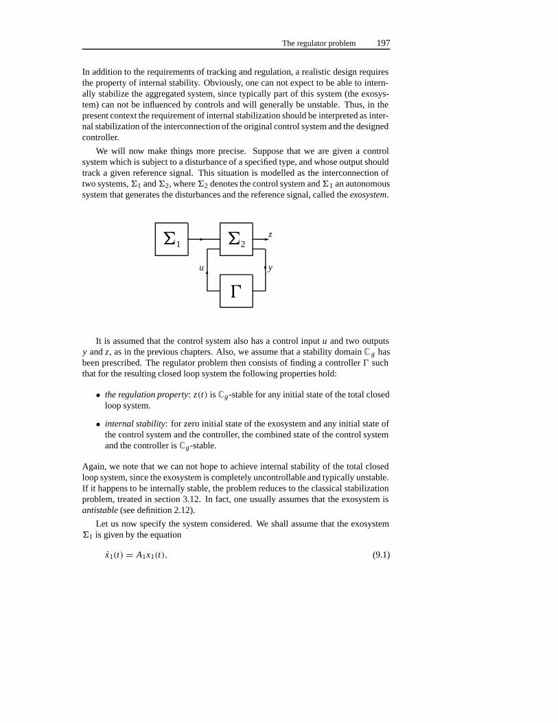
The regulator problem 197
In addition to the requirements of tracking and regulation, a realistic design requiresthe property of internal stability. Obviously, one can not expect to be able to intern-ally stabilize the aggregated system, since typically part of this system (the exosys-tem) can not be influenced by controls and will generally be unstable. Thus, in thepresent context the requirement of internal stabilization should be interpreted as inter-nal stabilization of the interconnection of the original control system and the designedcontroller.
We will now make things more precise. Suppose that we are given a controlsystem which is subject to a disturbance of a specified type, and whose output shouldtrack a given reference signal. This situation is modelled as the interconnection oftwo systems,�1 and�2, where�2 denotes the control system and�1 an autonomoussystem that generates the disturbances and the reference signal, called theexosystem.
�1� �2
��
�
�u y
z
It is assumed that the control system also has a control inputu and two outputsy andz, as in the previous chapters. Also, we assume that a stability domainC g hasbeen prescribed. The regulator problem then consists of finding a controller� suchthat for the resulting closed loop system the following properties hold:
• the regulation property: z(t) is Cg-stable for any initial state of the total closedloop system.
• internal stability: for zero initial state of the exosystem and any initial state ofthe control system and the controller, the combined state of the control systemand the controller isCg-stable.
Again, we note that we can not hope to achieve internal stability of the total closedloop system, since the exosystem is completely uncontrollable and typically unstable.If it happens to be internally stable, the problem reduces to the classical stabilizationproblem, treated in section 3.12. In fact, one usually assumes that the exosystem isantistable (see definition 2.12).
Let us now specify the system considered. We shall assume that the exosystem�1 is given by the equation
x1(t) = A1x1(t), (9.1)
198 Tracking and regulation
while the plant�2 is assumed to be given by the equations
x2(t) = A3x1(t) + A2x2(t) + B2u(t),y(t) = C1x1(t) + C2x2(t),z(t) = D1x1(t) + D2x2(t) + Eu(t).
(9.2)
The state spaceX2 of �2 is assumed to ben2-dimensional. The output spaceZ is r -dimensional. The disturbance enters the plant via the termA 3x1 in the state equationand via the termsC1x1 and D1x1 in the output equations. We allow for a directfeedthrough termEu from the control input to the to-be-controlled variable. Such aterm is omitted in the equation fory, because it would have been inconsequential forthe present problem.
It is convenient to combine�1 and�2 according to equations (9.1) and (9.2) toone system� with state variablex = (x T
1, x T
2)T and coefficient matrices
A : =(
A1 0A3 A2
), B : =
(0B2
), C : = (
C1 C2),
D : = (D1 D2
),
(9.3)
so that we have the following equations for� :
x(t) = Ax(t)+ Bu(t),y(t) = Cx(t),z(t) = Dx(t) + Eu(t).
(9.4)
Before investigating the existence of a controller with the desired properties, wedescribe what systems already satisfy the regulation property and the internal stabilitycondition. We define these properties for systems without control inputs, equivalently,for u = 0. We say that� is endostable if �2 is internally stable. This means that forx1(0) = 0 and arbitraryx2(0), the statex2(t) is Cg-stable. We say that� is (output)regulated if z(t) is Cg-stable for every initial state of�. These properties can beexpressed in terms of the coefficient matrices. Obviously,� is endostable if and onlyif σ(A2) ⊂ Cg . For output regulation, we have the following result.
Lemma 9.1 Assume that σ(A2) ⊂ Cg. Then the system � with input u = 0 is outputregulated if the equations
T A1− A2T = A3,
D2T + D1 = 0(9.5)
in T are solvable. If A1 is antistable, this condition is also necessary.
If A1 is not antistable then we can delete the stable part since it does not effectregulation which is only an asymptotic condition. In this way we can basically reducethe general problem to the case whenA1 is antistable.
Proof : The main idea is that for larget , the statex 2 of the plant is close toT x1, for asuitable linear mapT . So we introduce the variablev : = x 2−T x1, where we specify
The regulator problem 199
T later on. In a straightforward calculation, one derives from the equations (9.1) and(9.2) that
v(t) = A2v(t) + (A2T − T A1+ A3)x1(t) ,z(t) = D2v(t)+ (D1+ D2T )x1(t) .
(9.6)
Now assume thatT is a solution of the equations (9.5). Then the equations (9.6)reduce to
v(t) = A2v(t),z(t) = D2v(t).
SinceA2 is Cg-stable, theorem 3.23 implies thatz(t) is Cg-stable.
Conversely, assume thatA1 is antistable and that the system� is regulated andendostable. Then it follows from Sylvester’s Theorem (see section 9.3) that thereexists a (unique) matrixT satisfying the first equation of (9.5). Substituting thisinto (9.6), we find thatv(t) is Cg-stable. Sincez(t) is alsoCg-stable, this impliesthat(D2T + D1)x1(t) is Cg-stable. However, becausex1 is antistable for any initialcondition, we must have thatD2T + D1 = 0.
Now we want to solve the regulator problem by constructing a controller such thatthe closed loop system satisfies the conditions of lemma 9.1. As usual, the controller� will be of the form
w(t) = Kw(t) + Ly(t),u(t) = Mw(t) + Ny(t).
(9.7)
The closed loop system will be equal to the cascade connection� cl of �1 and�2,cl ,where�2,cl is the feedback interconnection of�2 and�, given by
x2e(t) = A2ex2e(t) + A3ex1(t),z(t) = D1ex1(t) + D2ex2e(t),
where
A2e : =(
A2+ B2NC2 B2MLC2 K
), A3e : =
(A3+ B2NC1
LC1
),
D2e : =(D2 + E NC2 E M
), D1e : = D1 + E NC1.
(9.8)
We call � a regulator if �cl is endostable and output regulated. The problem offinding a regulator will be called theregulator problem. It follows from lemma 9.1that the regulator problem can be solved by finding� = (K , L,M, N) such thatA 2e
is stable and the equations
Te A1− A2eTe = A3e , D2eTe + D1e = 0 (9.9)
have a solutionTe. The existence of a solutionTe is necessary for the existence of aregulator if A1 is antistable. In order to be able to solve this problem we shall maketwo assumptions:
200 Tracking and regulation
• �2 is stabilizable withu as input, i.e.,(A2, B2) is stabilizable.
• � is detectable withy as output, i.e.,(C, A) is detectable
Obviously, the stabilizability of�2 is necessary for the existence of a regulator. Alsothe detectability of�2 is necessary. However, here we impose a more restrictivecondition on the system, viz. the detectability of the total system�. Note that thereexists a standard reduction technique to solve the problem when� 2 is detectable but� is not detectable. In an appropriate manner, this technique deletes the undetectablemodes and only requires us to design a suitable regulator for the remaining systemwhich satisfies the stronger condition of detectability we impose in this chapter. Fordetails we refer to [44,159]. Then we have the following result:
Theorem 9.2 Assume that (A2, B2) is stabilizable and (C, A) is detectable. Thenthere exists a regulator if the equations
T A1− A2T − B2V = A3,
D1 + D2T + EV = 0(9.10)
have a solution (T, V ). If A1 is antistable, the solvability of (9.10) is necessary forthe existence of a regulator. Specifically, if G : Y → X is such that σ(A + GC) ⊂Cg, F2 : X → U is such that σ(A2 + B2F2) ⊂ Cg and if F1 := −F2T + V ,F : = (F1 F2), where (T, V ) is a solution of (9.10), then a regulator is given by
w(t) = (A + GC + B F)w(t)− Gy(t),u(t) = Fw(t).
(9.11)
Proof : Assume thatA1 is antistable and that a regulator exists. This regulator sat-isfies (9.9) for someTe. We decomposeTe into Te = (T T,U T)T and substitute (9.8)into (9.9). The first block row of the first of the resulting equations reads:
T A1− (A2+ B2NC2)T − B2MU = A3+ B2NC1
and the second equation reads:
D1+ (D2 + E NC2)T + E MU + E NC1 = 0.
These relations show that(T, NC2T + MU + NC1) is a solution of (9.10).
Conversely, assume that(T, V ) satisfies (9.10). Define a controller� by
(K , L,M, N) : = (A + GC + B F,−G, F,0)
i.e., by (9.11) whereF andG satisfy the conditions of theorem 9.2. We claim that�
is a regulator. To show this, we have to prove that the resulting extended system isendostable, and that we have the regulation property. In order to prove endostability,we introducer : = w − x and notice thatx andr satisfy
x(t) = (A + B F)x(t) + B Fr(t) ,r(t) = (A + GC)r(t) .
Well-posedness of the regulator problem 201
Obviously,r(t) is Cg-stable. Ifx1(0) = 0 (and hencex1(t) = 0 for all t), the firstequation reduces to
x2(t) = (A2+ B2F2)x2(t)+ B2Fr(t).
Then we also havex2(t) is Cg-stable (compare theorem 2.7). Next we verify that�e is output regulated. To this extent, we defineU : = (I, T T)T and we claim thatTe : = (T T,U T)T satisfies (9.9). To show this, we substitute this and (9.8) into (9.9).Then for the first equation of (9.9) we have to prove that(
TU
)A1−
(A2 B2F
−GC2 A + GC + B F
)(TU
)=
(A3
−GC1
).
We notice thatFU = V . Hence the first block equation is exactly the first equationof (9.10), viz.T A1− A2T − BV = A3. The second equation takes some more effort.It reads:
G(C1+ C2T − CU)+U A1− AU − BV = 0.
The expression between parentheses equals zero because of the definition ofU . Theremaining terms are decomposed according to (9.3):(
IT
)A1−
(A1 0A3 A2
)(IT
)−
(0B2
)V =
(A1− A1
T A1− A3− A2T − B2V
)= 0,
where we have used the first equation of (9.10). This shows that the first equation of(9.9) is satisfied.
Next we consider the second equation of (9.9). It readsD 1 + D2T + EV = 0,which is the same as the second equation of (9.10) and hence it is immediately clearthat this is also satisfied.
9.2 Well-posedness of the regulator problem
A mathematical problem is calledwell posed if it is solvable and it remains solvableafter a small perturbation of the data of the problem. The equationx 2+ y2−ay+b =0, for example, is solvable (inR2) for a = 2 andb = 1, but it is not well posed forthese values ofa andb because the solvability is lost whenb is replaced by 1+ ε forarbitraryε > 0. The investigation of the well-posedness is easy for linear equations.As a matter of fact, we have
Lemma 9.3 Let X and Y be finite-dimensional linear spaces and let A : X→ Y bea linear map and b ∈ Y. Then the equation Ax = b in the variable x is well posed ifand only if A is surjective.
202 Tracking and regulation
Proof : If A is surjective, any matrix representation ofA will have a nonzero sub-determinant of dimension equal to the number of rows. Since this determinant is acontinuous function of the entries of the matrix (in fact, a polynomial) it follows thatit will remain nonzero when the entries are perturbed a little bit. Hence,A will remainsurjective, after a small perturbation. Therefore, the equationAx = b remains solv-able for small perturbations ofA andb. Obviously,b can be perturbed in an arbitraryway and not just locally.
Conversely, ifA is not surjective, imA is a proper subspace ofY. The equationAx = b is solvable if and only ifb ∈ im A. However,b cannot be an interior pointof im A, since imA contains no interior points. Consequently, an arbitrary smallperturbation ofb may take it out of imA and hence destroy the solvability of theequation.
Remark 9.4 In concrete situations, it is of importance to specify more precisely whatthe ‘data’ of the problem is. Sometimes not all of the entries in a matrix are considereddata and subject to perturbations. For example, ifA is a companion matrix, only thelast row is considered data. The remaining entries consist of ‘hard’ zeros and ones. Itfollows from the above proof that the necessity of the surjectivity ofA still holds ifonly the vectorb is considered data.
Remark 9.5 Usually, and in particular in the case of lemma 9.3, the well-posednessproblem is easier to solve than the original equation. It is easier to verify the surjec-tivity of a mapA than to examine the solvability of the equationAx = b.
We want to apply the above result to the regulator problem. For the solvabilityof the regulator problem, a number of conditions are imposed. In the first place, itis assumed that�2 is stabilizable and� detectable. It is not difficult to see thatthese properties are invariant under small perturbations. For instance, if(A, B) isstabilizable andF is a stabilizing feedback, thenA + B F is a stability matrix. Sincethe eigenvalues depend continuously on the matrix,A+ B F is also a stability matrixif A and B are close toA andB. The important part to check is the well-posednessof the matrix linear equation (9.10). For this, we apply the previous theorem. We findthat the equation:
T A1− A2T − B2V = A3,
D2T + EV = −D1
in the variablesT andV is well posed if and only if the map
(T, V ) �→ (T A1− A2T − B2V, D2T + EV )
is surjective. In order to check this condition, one can give a matrix representationof this map using tensor products. We will however follow a different procedure,based on general considerations on the solvability of matrix equations. The advantageof the condition thus obtained will be that it can be interpreted in systemic terms,specifically, in terms of the zeros of a system.
Linear matrix equations 203
9.3 Linear matrix equations
The subject of this section is the solvability of linear matrix equations of the form
k∑i=1
Ai X Bi = C, (9.12)
whereAi , Bi andC are given matrices andX is unknown. We distinguish betweenuniversal and individual solvability of (9.12). We say that (9.12) isuniversally solv-able if the equation has a solution for everyC . Universal solvability thus is a con-dition on the matricesAi and Bi . If we want to stress that the equation is solvablefor the particularC given, we say that (9.12) isindividually solvable. Conditions forsolvability can be given by viewing the left-hand side of (9.12) as a linear mapLacting on the matrixX . Then (9.12) is individually solvable if and only ifC ∈ im L,and (9.12) is universally solvable if and only ifL is surjective. One can give explicitconditions for these properties using tensor (or Kronecker) products, but this will giverise to huge matrices and little insight. Rather, we would like to have results in thespirit of Sylvester’s theorem: the equation AX−X B = C, where A and B are squarematrices, is universally solvable if and only if σ(A) ∩ σ(B) = ∅. It does not seempossible to obtain a similar result for the general equation (9.12). However, if werestrict ourselves to the case where the matricesBi are of the formBi = qi (B) forgiven polynomialsqi and a fixed matrixB, we can derive the following:
Theorem 9.6 Let Ai ∈ Rn×m , B ∈ Rp×p , and let qi (s) be polynomials for i =1, . . . , k. Let
A(s) : =k∑
i=1
Ai qi (s). (9.13)
Then the equation
k∑i=1
Ai Xqi (B) = C, (9.14)
is universally solvable if and only if rankA(λ) = n for all λ ∈ σ(B).It is straightforward that Sylvester’s theorem is a special case of this result.
Proof : (‘only if’:) Suppose that rankA(λ) < n for someλ ∈ σ(B). Choose nonzerovectorsv andw such thatBv = λv andwT A(λ) = 0. Then we have for any matrixX :
wT∑
Ai Xqi (B)v = wT∑
Ai Xqi (λ)v = wT A(λ)Xv = 0.
Hence, ifwTCv = 0 (e.g. ifC = wvT), (9.14) does not have a solution.
204 Tracking and regulation
(‘if’:) The polynomial matrix A(s) is obviously right invertible as a rational ma-trix. Hence there exists a polynomial matrixD(s) and a scalar polynomiala(s) suchthatA(s)D(s) = a(s)I , wherea(s) is the product of the invariant factors ofA(s). Theassumption of the theorem implies thata(λ) = 0 forλ ∈ σ(B), hence, by the spectralmapping theorem (see (2.11)), thata(B) is nonsingular. DefiningC 1 : = C(a(B))−1
andE(s) : = D(s)C1 we find
k∑i=1
Ai E(s)qi (s) = A(s)E(s) = C1a(s).
Next we apply right substitution ofs = B into this equation and use theorem 7.6.This yields
∑ki=1 Ai Er (B)qi (B) = C1a(B) = C , which shows thatX : = Er (B)
(the indexr indicates right substitution) is a solution of (9.14).
Next we investigate the individual solvability of equation (9.14). For the equa-tions AX − X B = C and AX − Y B = C , such conditions were given by Roth in1952, viz.
Theorem 9.7
(i) Let A, B and C be matrices such that the equation AX − X B = C is defined.Then this equation has a solution if and only if the matrices(
A 00 B
)and
(A C0 B
)
are similar.
(ii) If A, B and C are polynomial matrices of dimensions such that the equationsAX − Y B = C makes sense, then this equation has a (polynomial matrix)solution if and only if(
A 00 B
)and
(A C0 B
)
are unimodularly equivalent.
An elegant proof of these theorem can be found in [80, Theorem 4.4.22]. We wantto generalize this result to the equation (9.14). A generalization in terms of similarityseems difficult. However, it is known that two matricesA and A are similar if andonly if the polynomial matricess I − A and s I − A are unimodularly equivalent.Hence, according to Roth, the equationAX − X B = C is solvable if and only if thepolynomial matrices(
s I − A 00 s I − B
)and
(s I − A C
0 s I − B
)
are unimodularly equivalent. This formulation has a direct generalization:
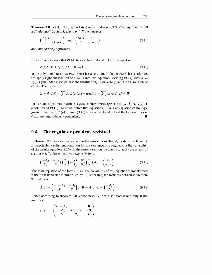
The regulator problem revisited 205
Theorem 9.8 Let Ai , B, qi(s) and A(s) be as in theorem 9.6. Then equation (9.14)is (individually) solvable if and only if the matrices(
A(s) 00 s I − B
)and
(A(s) C
0 s I − B
)(9.15)
are unimodularly equivalent.
Proof : First we note that (9.14) has a solution if and only if the equation
A(s)P(s)+ Q(s)(s I − B) = C (9.16)
in the polynomial matricesP(s), Q(s) has a solution. In fact, if (9.16) has a solution,we apply right substitution ofs = B into this equation, yielding (9.14) withX =Pr (B) (the indexr indicates right substitution). Conversely, letX be a solution of(9.14). Then we write:
C − A(s)X =∑
i
Ai X (qi (B)− qi (s)I ) =∑
i
Ai Vi (s)(s I − B)
for certain polynomial matricesVi (s). Hence(P(s), Q(s)) : = (X,∑
Ai Vi (s)) isa solution of (9.16). Next we notice that equation (9.16) is an equation of the typegiven in theorem 9.7 (ii). Hence (9.16) is solvable if and only if the two matrices in(9.15) are unimodularly equivalent.
9.4 The regulator problem revisited
In theorem 9.2, we saw that subject to the assumptions that�2 is stabilizable and�is detectable, a sufficient condition for the existence of a regulator is the solvabilityof the matrix equation (9.10). In the present section, we intend to apply the results ofsection 9.3. To this extent, we rewrite (9.10) to(−A2 −B2
D2 E
)(TV
)+
(I 00 0
)(TV
)A1 =
(A3−D1
). (9.17)
This is an equation of the form (9.14). The solvability of this equation is not affectedif the right-hand side is multiplied by -1. After this, the matrices defined in theorem9.6 reduce to
A(s) =(
s I − A2 −B2D2 E
), B = A1, C =
(−A3D1
). (9.18)
Hence according to theorem 9.8, equation (9.17) has a solution if and only if thematrices
P(s) : =s I − A1 0 0−A3 s I − A2 −B2D1 D2 E
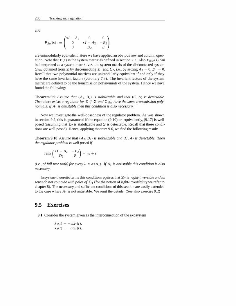
206 Tracking and regulation
and
Pdisc(s) : =s I − A1 0 0
0 s I − A2 −B20 D2 E
are unimodularly equivalent. Here we have applied an obvious row and column oper-ation. Note thatP(s) is the system matrix as defined in section 7.2. AlsoPdisc(s) canbe interpreted as a system matrix, viz. the system matrix of the disconnected system�disc obtained from� by disconnecting�1 and�2, i.e., by settingA3 = 0, D1 = 0.Recall that two polynomial matrices are unimodularly equivalent if and only if theyhave the same invariant factors (corollary 7.3). The invariant factors of the systemmatrix are defined to be the transmission polynomials of the system. Hence we havefound the following:
Theorem 9.9 Assume that (A2, B2) is stabilizable and that (C, A) is detectable.Then there exists a regulator for � if � and �disc have the same transmission poly-nomials. If A1 is antistable then this condition is also necessary.
Now we investigate the well-posedness of the regulator problem. As was shownin section 9.2, this is guaranteed if the equation (9.10) or, equivalently, (9.17) is wellposed (assuming that�2 is stabilizable and� is detectable. Recall that these condi-tions are well posed). Hence, applying theorem 9.6, we find the following result:
Theorem 9.10 Assume that (A2, B2) is stabilizable and (C, A) is detectable. Thenthe regulator problem is well posed if
rank
(λI − A2 −B2
D2 E
)= n2+ r
(i.e., of full row rank) for every λ ∈ σ(A1). If A1 is antistable this condition is alsonecessary.
In system-theoretic terms this condition requires that�2 is right-invertible and itszeros do not coincide with poles of �1 (for the notion of right-invertibility we refer tochapter 8). The necessary and sufficient conditions of this section are easily extendedto the case whereA1 is not antistable. We omit the details. (See also exercise 9.2)
9.5 Exercises
9.1 Consider the system given as the interconnection of the exosystem
x1(t) = −ωx2(t),x2(t) = ωx1(t),
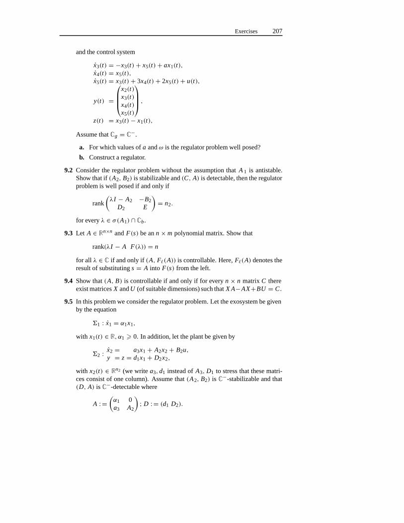
Exercises 207
and the control system
x3(t) = −x3(t)+ x5(t)+ ax1(t),x4(t) = x5(t),x5(t) = x3(t)+ 3x4(t)+ 2x5(t)+ u(t),
y(t) =
x2(t)x3(t)x4(t)x5(t)
,
z(t) = x3(t)− x1(t),
Assume thatCg = C−.
a. For which values ofa andω is the regulator problem well posed?
b. Construct a regulator.
9.2 Consider the regulator problem without the assumption thatA 1 is antistable.Show that if(A2, B2) is stabilizable and(C, A) is detectable, then the regulatorproblem is well posed if and only if
rank
(λI − A2 −B2
D2 E
)= n2.
for everyλ ∈ σ(A1) ∩ Cb.
9.3 Let A ∈ Rn×n andF(s) be ann ×m polynomial matrix. Show that
rank(λI − A F(λ)) = n
for all λ ∈ C if and only if (A, F�(A)) is controllable. Here,F�(A) denotes theresult of substitutings = A into F(s) from the left.
9.4 Show that(A, B) is controllable if and only if for everyn × n matrix C thereexist matricesX andU (of suitable dimensions) such thatX A−AX+BU = C .
9.5 In this problem we consider the regulator problem. Let the exosystem be givenby the equation
�1 : x1 = α1x1,
with x1(t) ∈ R, α1 � 0. In addition, let the plant be given by
�2 : x2 = a3x1+ A2x2+ B2u,y = z = d1x1+ D2x2,
with x2(t) ∈ Rn2 (we writea3, d1 instead ofA3, D1 to stress that these matri-ces consist of one column). Assume that(A2, B2) is C−-stabilizable and that(D, A) is C−-detectable where
A : =(α1 0a3 A2
); D : = (d1 D2).
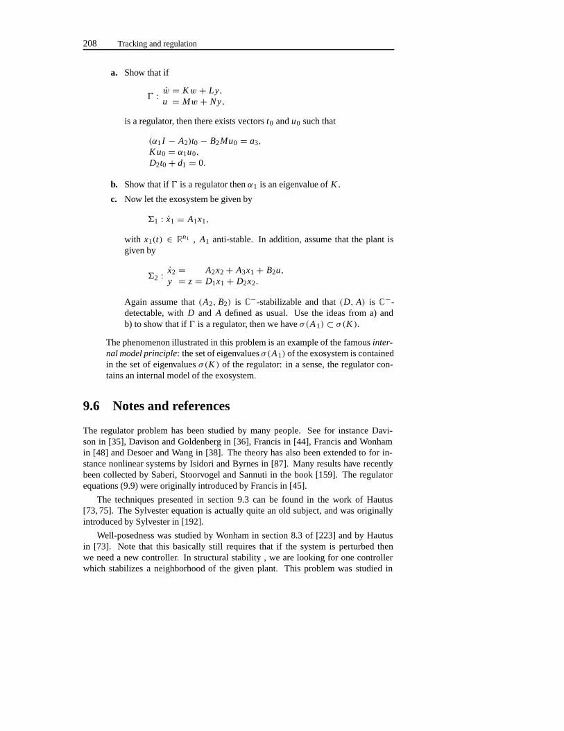
208 Tracking and regulation
a. Show that if
� : w = Kw + Ly,u = Mw + Ny,
is a regulator, then there exists vectorst0 andu0 such that
(α1I − A2)t0 − B2Mu0 = a3,
K u0 = α1u0,
D2t0+ d1 = 0.
b. Show that if� is a regulator thenα1 is an eigenvalue ofK .
c. Now let the exosystem be given by
�1 : x1 = A1x1,
with x1(t) ∈ Rn1 , A1 anti-stable. In addition, assume that the plant isgiven by
�2 : x2 = A2x2+ A3x1+ B2u,y = z = D1x1+ D2x2.
Again assume that(A2, B2) is C−-stabilizable and that(D, A) is C−-detectable, withD and A defined as usual. Use the ideas from a) andb) to show that if� is a regulator, then we haveσ(A 1) ⊂ σ(K ).
The phenomenon illustrated in this problem is an example of the famousinter-nal model principle: the set of eigenvaluesσ(A1) of the exosystem is containedin the set of eigenvaluesσ(K ) of the regulator: in a sense, the regulator con-tains an internal model of the exosystem.
9.6 Notes and references
The regulator problem has been studied by many people. See for instance Davi-son in [35], Davison and Goldenberg in [36], Francis in [44], Francis and Wonhamin [48] and Desoer and Wang in [38]. The theory has also been extended to for in-stance nonlinear systems by Isidori and Byrnes in [87]. Many results have recentlybeen collected by Saberi, Stoorvogel and Sannuti in the book [159]. The regulatorequations (9.9) were originally introduced by Francis in [45].
The techniques presented in section 9.3 can be found in the work of Hautus[73, 75]. The Sylvester equation is actually quite an old subject, and was originallyintroduced by Sylvester in [192].
Well-posedness was studied by Wonham in section 8.3 of [223] and by Hautusin [73]. Note that this basically still requires that if the system is perturbed thenwe need a new controller. In structural stability , we are looking for one controllerwhich stabilizes a neighborhood of the given plant. This problem was studied in
Notes and references 209
many variations and has been studied by Francis, Sebakhy and Wonham in [47], byDavison and Goldenberg in [36], by Desoer and Wang in [38], by Pearson, Shieldsand Staats in [142] and by Francis and Wonham in [48]. More recently the knownresults were extended by Saberi, Stoorvogel and Sannuti in the book [159].
The internal model principle studied by Wonham in [223] and by Francis andWonham in [48] was only for the case that the to be regulated signal is equal to themeasurement signal. Extensions to the general case can be found in the book [159]by Saberi, Stoorvogel and Sannuti. Note that the internal model principle is unrelatedto well-posedness, structural stability (which is sometimes also referred to as robustregulation) which is sometimes alluded to in the literature. It is a basic propertyresulting directly from the fact that we achieve regulation.

210 Tracking and regulation
Chapter 10
Linear quadratic optimalcontrol
In the previous chapters we have been concerned with control problems that requirethe controlled system to satisfy specific, qualitative, properties, such as internal sta-bility, the property of being disturbance decoupled, external stability, the regulationproperty, etc.. In the present chapter we will take into accountquantitative aspects.Given a control system, we will express the performance of the controlled system interms of a cost functional. The control problem will then be to find all optimal con-trollers i.e, all controllers that minimize the cost functional. Such controllers lead toa controlled system with optimal performance.
10.1 The linear quadratic regulator problem
Consider the control system� given by the equations
x(t) = Ax(t)+ Bu(t),z(t) = Cx(t)+ Du(t).
(10.1)
Here,u is the control input, andz is the output to be controlled. We assume thatutakes its values inU, which we identify withRm , andz takes its values inZ, to beidentified withRp. The statex is assumed to take its values inX, to be identifiedwith Rn .
We now explain what we mean by a disturbance. By a disturbance we meanthe occurrence of an ‘initial state’x(0) = x0. This could alternatively be modelledby replacing the differential equation of� by x = Ax + Bu + δx 0, whereδx0 isinterpreted as a disturbance input.
Suppose that it is desired to keep all components of the outputz(t) as small aspossible, for allt . In the ideal situation, the uncontrolled system (u = 0) evolvesalong the stationary solutionx = 0. Of course, the outputz(t) will then also be
212 Linear quadratic optimal control
equal to zero for allt . Suppose now that at timet = 0 the state of the system isperturbed to, say,x(0) = x0. After the occurrence of this impulsive disturbance,the uncontrolled system will evolve along a state trajectory unequal to the stationaryzero solution, and we will getz(t) = Ce At x0. If, however, from timet = 0 on, weapply an input functionu, then fort � 0 the corresponding output becomes equal toz(t) = Cx(t) + Du(t). Keeping in mind that we want the outputz(t) to be as smallas possible for allt � 0, we measure its size by the quadratic cost functional
J (x0, u) =∫ ∞
0‖z(t)‖2 dt, (10.2)
where‖ ·‖ denotes the Euclidean norm. Our desire to keep the values of the output assmall as possible can be expressed by requiring this integral to be as small as possibleby suitable choice of input functionu. In this way we arrive at thelinear quadraticregulator problem:
Problem 10.1 Consider the system� : x(t) = Ax(t)+Bu(t), z(t) = Cx(t)+Du(t).Determine for every initial state x0 an input u ∈ U (a space of functions [0,∞) →U) such that
J (x0, u) : =∫ ∞
0‖z(t)‖2 dt (10.3)
is minimal. Here z(t) denotes the output trajectory zu(t, x0) of � corresponding tothe initial state x0 and input function u.
Since the system is linear and the integrand in the cost functional is a quadraticfunction of z, the problem is calledlinear quadratic. Of course,‖z‖ 2 = x TCTCx +2uT DTCx + uT DT Du, so the integrand can also be considered as a quadratic functionof (x, u).
In the problem formulation, we are not explicit about the exact nature ofU. Infact, like in the previous chapters, it is not very important whatU is. One can takee.g. the space of piecewise continuous functions, the space of piecewise smooth (i.e.piecewiseC∞) functions or the space of locally integrable functions. In the last case,one has to interpret the various formulas in a measure-theoretic sense (in particular,formulas containing derivatives have to be understood to hold ‘almost everywhere’).
Of course, the convergence of (10.3) is a point of concern. Therefore, one oftenconsiders the correspondingfinite horizon problem in a preliminary investigation. Inthis problem, a final timeT is given and one wants to minimize the integral
J (x0, u, T ) : =∫ T
0‖z(t)‖2 dt . (10.4)
In contrast to this, the first problem above is sometimes called theinfinite horizonproblem.
An important issue is the convergence of the state. Obviously, convergence of theintegral does not always imply the convergence to zero of the state. Therefore, dis-tinction is made between the problem with zero and with free endpoint. Problem 10.1
The linear quadratic regulator problem 213
as stated is referred to as theproblem with free endpoint. If one restricts the inputsu in the problem to those for which the resulting state trajectory tends to zero, onespeaks about theproblem with zero endpoint. Specifically:
Problem 10.2 In the situation of problem 10.1, determine for every initial state x 0an input u ∈ U such that x(t) → 0 (t → ∞) and such that under this condition,J (x0, u) is minimized.
Remark 10.3 There is a special situation where the linear quadratic regulator pro-blem (with free endpoint) is very easily solved. This is the case wherex 0 ∈ V(�),the weakly unobservable subspace (see chapter 7). In fact, in this case, there existsa controlu ∈ U such that the output is identically zero. Such a control is obvi-ously optimal. This control can be given by the state feedbacku = Fx , whereF : = −(DT D)−1DTC . Likewise, the problem with zero endpoint is very easilysolved if x0 ∈ Vg(�), the stabilizable weakly unobservable subspace, with stabilitydomainCg equal toC− (see exercise 7.16). In that case there exists a control suchthat the output is zero, and the state converges to zero ast tends to infinity. Thiscontrol is optimal.
Various special cases of these problems have been considered in the literature. Inthe literature names have been associated to these special cases.
Definition 10.4 Problems 10.1 and 10.2 are called regularif D is injective, equiv-alently, DT D > 0. The problem is said to be in standard formif C T D = 0 andDT D = I .
In the standard case, the integrand in the cost functional reduces to‖z‖ 2 =x TCTCx + uTu. We often writeQ = C TC .
One of the issues to be addressed is the existence of optimal controls. Since forany initial state and any input functionu we haveJ (x 0, u) � 0, also J ∗(x0) : =inf{J (x0, u) | u ∈ U} � 0. Thus one is at least assured of the boundedness frombelow of the infimum of the integral. This, however, does not immediately imply theexistence of an optimal control, since the infimum might not be attained. In general,solutions do not exist within the class of ordinary functions unlessD T D > 0, i.e. theproblem is regular. In the situation where this condition is not satisfied, one has toextend the set of admissible input functions to distributions. Henceforth, we restrictourselves to the regular case.
The standard case is a special case, which is not essentially simpler than the gen-eral regular problem, but which gives rise to simpler formulas. The general regularproblem can be reduced to the standard case by means of a feedback transforma-tion, that is, by the introduction of a new control variablev which is related tou byu = Fx + Gv, where
F : = −(DT D)−1DTC andG : = −(DT D)−12 .
214 Linear quadratic optimal control
Indeed, after this preliminary feedback transformation and transformation of the inputspace, the original system is transformed to
x(t) = (A + B F)x(t)+ BGv(t),z(t) = (C + DF)x(t)+ DGv(t),
which gives rise to a standard problem since(DG)T(C+DF) = 0 and(DG)T DG =I .
It is not very difficult to show that the infimum ofJ is a quadratic function ofx 0,provided it is finite. We will not do this because it will be a result of our calculationsanyway. However, the statement is made here because it will be a heuristic motivationof some of the steps in the treatment of the problems. It is very easy to see that, ifJ ∗(x0) = inf{J (x0, u) | u ∈ U} is finite, thenJ ∗(λx0) = λ2J ∗(x0), which makes itplausible thatJ ∗(x0) is a quadratic function.
10.2 The finite-horizon problem
We start from the standard problem:
Problem 10.5 Given the system x(t) = Ax(t) + Bu(t), a final time T > 0, andsymmetric matrices N and Q such that N � 0 and Q � 0, determine for every initialstate x0 a piecewise continuous input function u : [0, T ] → U such that the integral
J (x0, u, T ) : =∫ T
0x(t)T Qx(t)+ u(t)Tu(t) dt + x(T )T Nx(T ) (10.5)
is minimized.
In this problem, we have introduced a weight on the final state, using the matrixN . This generalization of the problem can be dealt with without any effort.
As remarked at the end of the previous section, the minimal value ofJ is expectedto be a quadratic function ofx0, sayx T
0K x0. More generally, we expect that the mini-
mum of the integral∫ T
t0x T Qx+uTu dt is of the formx T
0K (t0)x0. We now assume thatK (t) is any symmetric-matrix-valued continuously differentiable function, defined on[0, T ] and we have in mind the interpretation ofK given in the previous sentence. Weconsider the differenceJ (x0, u, T )− x T
0K (0)x0 for any admissible inputu. Then wehave
J (x0, u, T )− x T
0K (0)x0 =∫ T
0x(t)T Qx(t)+ u(t)Tu(t) dt
+∫ T
0
d
dtx(t)T K (t)x(t) dt + x(T )T(N − K (T ))x(T ).
The finite-horizon problem 215
We take the two integrals together and compute the second integral using the differ-ential equation. The integrand will be (we omit the dependence ont):
x T Qx + uTu + d
dtx T K x = x T(Q + AT K + K A + K )x + 2uT BT K x + uTu
= x T K B BTK x + 2uT BT K x + uTu + x TSx
= ‖u + BT K x‖2+ x TSx,
where
S : = K + AT K + K A − K B BTK + Q.
In the computations, we have completed the square. As a result, we get
J (x0, u, T ) = x T
0K (0)x0+∫ T
0[x(t)TS(t)x(t)+ ‖u(t)+ BT K (t)x(t)‖2] dt
+ x(T )T(N − K (T ))x(T ). (10.6)
This formula will play a crucial role in our further treatment. It will be referred to asthe completion of squares formula. A primitive attempt to minimize the integral in(10.5) is to chooseu such that the integrand is minimized for every value oft . Thisdoes not work, because the choice ofu is going to affect the values ofx for largert , and it is difficult to predict what the total effect onJ will be. A similar situationprevails when we try to minimize (10.6) in this way, unless we choose the matrixKin a particular way. In fact, if we are able to chooseK such thatS(t) is identicallyzero andK (T ) = N , the expression forJ reduces to
J (x0, u, T ) = x T
0K (0)x0+∫ T
0‖u(t)+ BT K (t)x(t)‖2 dt . (10.7)
It is obvious from this expression thatJ (x0, u, T ) � x T
0K (0)x0 for all u and thatequality is achieved if and only ifu(t) = −B TK (t)x(t) for all t ∈ [0, T ]. Thus wehave obtained the following result:
Theorem 10.6 Let K : [0, T ] → Rn×n be continuously differentiable and such thatK (t) is symmetric for every t ∈ [0, T ]. If K is a solution of the Riccati equation:
K (t) = −AT K (t)− K (t)A + K (t)B BT K (t)− Q (10.8)
with final condition K (T ) = N, then for each initial state x0 we have
J ∗(x0, T ) : = inf{J (x0, u, T ) | u piecewise continuous on [0, T ]} = x T
0K (0)x0
(10.9)
Furthermore, for a given initial state x0, an input function u is optimal, i.e., u ispiecewise continuous on [0, T ] and J (x0, u, T ) = J ∗(x0, T ), if and only if
u(t) = −BT K (t)x(t), 0 � t � T . (10.10)
216 Linear quadratic optimal control
Assuming for the moment thatK satisfying the desired properties can be found,we obtain an optimal control as a time-varying feedback (see (10.10)). For a giveninitial state, we can construct anopen-loop control function by substituting (10.10)into the differential equation. This yields a time varying linear autonomous equation:x(t) = (A−B BTK (t))x(t) with initial statex(0) = x0. Such an initial value problemis well known to have a unique solution on any time interval. If the solution is denotedwith ξ(t) then the open-loop formula foru is u(t) = −B T K (t)ξ(t). Thus we see thatfor each initial statex0 there is a unique optimal control input.
It follows that the optimization problem is solved when the Riccati equation issolved. This equation is a nonlinear initial (or rather final) value problem. The exis-tence of a solution of such a problem is not always guaranteed, as follows from theexamplex = x 2 + 1, which hasx(t) = tan(t + c) as a general solution. For noc,a solution exists over an interval larger thanπ . The general theory of ordinary dif-ferential equations only guarantees the existence of alocal solution, defined over aninterval whose length cannot be prescribed. Specifically:
Theorem 10.7 Let T > 0, x0 ∈ Rn, and let f : Rn × [0, T ] → Rn be continuouslydifferentiable. Then we have:
(i) There exists T1 satisfying 0 < T1 < T such that the differential equation withinitial condition
x(t) = f (x(t), t), x(0) = x0 (10.11)
has a solution on [0, T1].(ii) If (10.11) has a solution on some interval [0, T1], it is unique.
(iii) If the solution on each interval [0, T1], on which it exists, is bounded with abound independent of T1, then there exists a solution of (10.11) on [0, T ].
We apply this theorem to the Riccati equation and with the time reversed. Notethat this equation can be viewed as an equation of the type considered in theorem10.7. According to theorem 10.7, there exists a unique solutionK of
K (t) = −AT K (t)− K (t)A + K (t)B BTK (t)− Q, K (T ) = N . (10.12)
on some interval[T1, T ]. If we want to emphasize the dependence of this solutionon the final timeT we will write this solution asK (t, T ). Note also that, sinceNis symmetric, the matrix functionK T(t, T ) will satisfy (10.12). By uniqueness, itfollows thatK T(t, T ) = K (t, T ) for T1 � t � T . Using the special interpretation ofthe solution of the Riccati equation as minimal value of the integral, one can actuallyderive global existence of the solution:
Theorem 10.8 The Riccati equation with initial value, (10.12), has a unique solutionon the interval [0, T ] for every symmetric N. This solution is symmetric.
The finite-horizon problem 217
Proof : The only thing we have to prove is thatK (t, T ) is uniformly bounded oneach interval of its existence. Letx0 ∈ X be arbitrary and suppose thatK (t, T )exists on[T1, T ]. Choose the inputu identically zero on[0, T ]. Taket0 any elementof [T1, T ]. By time invariance, the functionL(t) : = K (t + t0, T ) is a solution of theRiccati equation on[0, T − t0]. Hence by theorem 10.6,x T
0L(0)x0 is the minimum ofJ (x0, u, T − t0) over allu. In particular,
x T
0K (t0, T )x0 = x T
0L(0)x0 � J (x0,0, T − t0).
Clearly,
J (x0,0, T − t0) =∫ T−t0
0x T
0eATt QeAt x0 dt + x T
0eAT(T−t0)NeA(T−t0)x0
�∫ T
0x T
0eATt QeAt x0 dt + x T
0eAT(T−t0)NeA(T−t0)x0.
Now, t �→ x T
0eA(T−t)NeA(T−t)x0 is a continuous function on the compact interval[0, T ] and is therefore bounded from above by a constant, sayM . Thus we concludethat x T
0K (t0, T )x0 is bounded from above by a constant, independent oft 0 andT1.This implies that the matrix functionK (t, T ) itself is bounded with a bound inde-pendent ofT1 (see also exercise 10.2). Hence according to theorem 10.7, the Riccatiequation has a solution on the total interval.
The dependence of the solutionK (t, T ) on botht andT is inconvenient if wewant to use the results of this section for the infinite horizon case. Fortunately,K isactually a function of one variable, specifically,T − t . In fact, if we defineP(t) : =K (T − t, T ), thenP satisfies the initial-value problem:
P(t) = AT P(t) + P(t)A − P(t)B BT P(t) + Q, P(0) = N . (10.13)
Obviously, the solution of this problem does not depend onT . We reformulate theresults of this section in terms ofP(t):
Theorem 10.9 Consider the system x(t) = Ax(t) + Bu(t), together with the costfunctional
J (x0, u, T ) : =∫ T
0x(t)T Qx(t)+ u(t)Tu(t) dt + x(T )T Nx(T ), (10.14)
where Q � 0 and N � 0, and furthermore, T > 0. Then we have the followingproperties:
(i) The Riccati equation with initial value
P(t) = AT P(t) + P(t)A − P(t)B BT P(t) + Q, P(0) = N, (10.15)
has a unique solution on [0,∞). This solution is symmetric and positivesemidefinite for all t � 0.
218 Linear quadratic optimal control
(ii) For each x0 there is exactly one optimal input function, i.e., a piecewise contin-uous function u∗ on [0, T ] such that J (x0, u∗, T ) = J ∗(x0, T ). This optimalinput function u∗ is generated by the time-varying feedback control law
u(t) = −BT P(T − t)x(t) (0 � t � T ). (10.16)
(iii) For each x0, the minimal value of the cost functional equals
J ∗(x0, T ) = x T
0P(T )x0.
(iv) If N = 0, then the function t �→ P(t) is an increasing function in the sensethat P(t) − P(s) is positive semidefinite for t � s.
The monotonicity statement onP is an easy consequence of the interpretation ofP as the matrix representing the minimal cost of the performance criterion (see (iii)).
Remark 10.10 There is a second monotonicity statement we can make. If we con-sider two optimal control problems with the same system and the sameQ matrix, butwith two matricesN1 andN2, satisfyingN1 � N2, then for everyx0, the functionJassociated withN1 will be larger than the functionJ corresponding toN 2. There willtherefore be a similar relation between the minimal costs. HencePN1(t) � PN2(t)for all t � 0.
10.3 The infinite-horizon problem, standard case
We consider the situation as described in theorem 10.9 withN = 0. An obviousconjecture is thatx T
0P(T )x0 converges to the minimal cost of the infinite-horizonproblem asT → ∞. The convergence ofx T
0P(T )x0 for all x0 is equivalent to theconvergence of the matrixP(T ) for T →∞ to some matrixP − (see exercise 10.2).Such a convergence does not always take place. For instance, if we consider thesystemx(t) = 0 with state spaceX = R, andQ = 1, we haveP(t) = 1, P(0) = 0,with solutionP(t) = t . This is not surprising because in this case, ifx(0) = c = 0,the integral to be minimized equals
∫∞0 x2(t) + u2(t) dt �
∫∞0 c2 dt = ∞ for all
inputsu. In order to achieve convergence, we make the following assumption: foreveryx0, there exists an inputu for which the integral
J (x0, u) : =∫ ∞
0x(t)T Qx(t)+ u(t)Tu(t) dt (10.17)
converges, i.e., for which the costJ (x 0, u) is finite. Obviously, for the problem tomake sense for allx0, this condition is necessary. It is easily seen that the stabilizabil-ity of (A, B) is a sufficient condition for the above assumption to hold (not necessary,take e.g.Q = 0). Take an arbitrary initial statex 0 and assume thatu is a functionsuch that the integral (10.17) is finite. We have for everyT > 0 that
x T
0P(T )x0 � J (x0, u, T ) � J (x0, u),
The infinite-horizon problem, standard case 219
which implies that for everyx0, the expressionx T
0P(T )x0 is bounded. This impliesthat P(T ) is bounded (see exercise 10.2). SinceP(T ) is increasing with respect toT , it follows that P− := limT→∞ P(T ) exists. SinceP satisfies the differentialequation (10.15), it follows that alsoP(t) has a limit ast →∞. It is easily seen thatthis latter limit must be zero. HenceP = P− satisfies the following equation:
AT P + P A − P B B T P + Q = 0. (10.18)
This is is called theAlgebraic Riccati Equation (ARE). Note that the solutions of thisequation are exactly the constant solutions of the Riccati differential equation. Theprevious consideration shows that the ARE has a positive semidefinite solutionP −.The solution is not necessarily unique, not even with the extra condition thatP � 0.
We would like to use the previous results in order to solve the infinite horizonproblem. For this purpose, an obvious method would be to find a positive semidefinitesolutionP of (10.18) and to use the controlu = −B T Px , obtained from (10.16) bytaking the limit forT →∞. Here we expect the optimal cost to bex T
0Px0. There aretwo points that have to be clarified, however. In the first place, because of the lackof uniqueness ofP, we do not know which solution of (10.18) to take. In the secondplace, even if we have found the correct solution of the ARE, it is not obvious that theproposed control actually is optimal. Both points are already settled in the followinglemma:
Lemma 10.11 Suppose that for every x0 there exists an input u ∈ U such thatJ (x0, u) <∞. Then we have:
(i) P− := limT→∞ P(T ) exists, where P is the solution of Riccati differentialequation (10.15) with N = 0.
(ii) P− is the smallest real symmetric positive semidefinite solution of the ARE(10.18). Hence, for every real symmetric P � 0 satisfying ARE, we haveP � P−.
(iii) For every u ∈ U, the following holds
J (x0, u) = x T
0P−x0+∫ ∞
0‖u(t)+ BT P−x(t)‖2 dt . (10.19)
(iv) For every x0, J ∗(x0) : = inf{J (x0, u) | u ∈ U} = x T
0P−x0. Furthermore, forevery x0, there is exactly one optimal input function, i.e., a function u ∗ ∈U suchthat J (x0, u∗) = J ∗(x0). This optimal input is generated by the time-invariantfeedback law u(t) = −B T P−x(t).
Proof : We have seen already that (i) holds and thatP − satisfies ARE. Assume thatP∗ � 0 is any solution of the ARE. ThenP ∗ is a constant solution of the Riccatidifferential equation. AlsoP(t) is a solution andP(0) = 0 � P ∗. Hence,P(t) � P∗for all t � 0 (see remark 10.10), and consequentlyP − = limt→∞ P(t) � P∗.
220 Linear quadratic optimal control
In order to prove (iii), we apply the completion of squares formula (10.6) withK (t) : = P(T − t), N : = 0 andu arbitrary. Then
J (x0, u, T ) = x T
0P(T )x0+∫ T
0‖u(t)+ BT P(T − t)x(t)‖2 dt .
Choose a fixedT0 > 0. Then we have forT > T0 that
∫ T
0‖u(t)+ BT P(T − t)x(t)‖2 dt
�∫ T0
0‖u(t)+ BT P(T − t)x(t)‖2 dt →
∫ T0
0‖u(t) + BT P−x(t)‖2 dt
for T →∞. Hence
lim infT→∞
∫ T
0‖u(t)+ BT P(T − t)x(t)‖2 dt �
∫ T0
0‖u(t) + BT P−x(t)‖2 dt
for all T0. This implies
lim infT→∞ J (x0, u, T ) � x T
0P−x0+∫ ∞
0‖u(t) + BT P−x(t)‖2 dt .
Conversely, if in the completion of squares formula we takeK (t) = P −, N = 0, andu arbitrary, then
J (x0, u, T ) = x T
0P−x0+∫ T
0‖u(t)+ BT P−x(t)‖2 dt − x(T )T P−x(T )
� x T
0P−x0+∫ ∞
0‖u(t) + BT P−x(t)‖2 dt . (10.20)
Combination of these inequalities yields (10.19).
Finally, (iv) is a direct consequence of (iii).
Notice that the minimality condition uniquely determines the matrixP −.
Remark 10.12 It follows from the previous proof thatx(T ) T P−x(T )→ 0 wheneverJ (x0, u) is finite. In particular, in the case thatP− is positive definite, we infer thatx(t)→ 0 for t →∞, wheneverJ (x0, u) <∞.
Although the lemma provides a solution to the infinite horizon problem, it is un-satisfactory because it starts from the assumption that for each initial state there is atleast one control input such that the corresponding cost is finite. In the remainder ofthis section, we establish necessary and sufficient conditions, in terms of the matricesA, B andQ, under which the finite cost assumption holds.
FactorizeQ = C TC and introduce the output
z(t) =(
C0
)x(t)+
(0I
)u(t). (10.21)
The infinite-horizon problem, standard case 221
Our cost can then be written asJ (x0, u) = ∫∞0 ‖z‖2 dt .
Now, from exercise 7.4, recall the concept of output stabilizability. In general, asystem� : x(t) = Ax(t)+Bu(t), z(t) = Cx(t)+Du(t) is calledoutput stabilizableif there exists a state feedback control lawu(t) = Fx(t) such that for each initialstatex0 the corresponding outputz F (t, x0) converges to zero ast tends to infinity.According to exercise 7.4, the system� = (A, B,C, D) is output stabilizable if andonly if
X = V(�)+Xstab, (10.22)
whereX is the state space of�, V(�) the weakly unobservable subspace, andX stabthe stabilizable subspace of(A, B) with respect to the stability domainC−.
We will apply this to the system� given by x(t) = Ax(t) + Bu(t), togetherwith the output equation (10.21). It is easily seen that for this special case we haveV(�) = 〈kerC | A〉 (see exercise 7.5), so the system� is output stabilizable if andonly if
X = 〈kerC | A〉 +Xstab.
It is clear that if� is output stabilizable then for any initial statex 0 there is acontrol inputu such thatJ (x0, u) < ∞. It follows from lemma 10.11 that also theconverse holds. Indeed, if for allx 0 there exists an inputu such thatJ (x0, u) < ∞,then for allu (10.19) holds. This implies that the feedback lawu(t) = Fx(t) withF : = −BT P− yields
∫∞0 ‖zF (t, x0)‖2 dt < ∞, for any initial statex0. This in turn
implies thatzF (t, x0)→ 0 (t →∞) for all x0, so the system� is output stabilizable.We conclude that the finite cost assumption of lemma 10.11 is equivalent to outputstabilizability of�.
It also follows from lemma 10.11 that the finite cost assumption implies the exis-tence of a real symmetric positive semidefinite solution of the ARE (10.18). We willnow show that also the converse holds. Indeed, assumeP is a positive semidefinitesolution of the ARE. Then (10.20) withP− replaced byP implies
J (x0, u, T ) � x T
0Px0 +∫ ∞
0‖u(t) + BT Px(t)‖2 dt,
for all T . By takingu(t) = Fx(t) with F : = −B T P we obtainJ (x0, u, T ) � x T
0Px0for all T and henceJ (x0, u) <∞.
Summarizing the above we obtain the following theorem:
Theorem 10.13Consider the system x(t) = Ax(t) + Bu(t) together with the costfunctional
J (x0, u) : =∫ ∞
0x(t)T Qx(t)+ u(t)Tu(t) dt,
with Q � 0. Factorize Q = C TC. Then the following statements are equivalent:
222 Linear quadratic optimal control
(i) For every x0 ∈ X there exists u ∈ U such that J (x0, u) <∞.
(ii) The ARE (10.18) has a real symmetric positive semidefinite solution P,
(iii) The system
� =(
A, B,(
C0
),
(0I
))is output stabilizable,
(iv) 〈kerC | A〉 +Xstab=X.
Assume that one of the above conditions holds. Then there exists a smallest realsymmetric positive semidefinite solution of the ARE, i.e., there exists a real symmetricsolution P− � 0 such that for every real symmetric solution P � 0 we have P− � P.For every x0 we have
J ∗(x0) : = inf{J (x0, u) | u ∈ U} = x T
0P−x0.
Furthermore, for every x0, there is exactly one optimal input function, i.e., a functionu∗ ∈ U such that J (x0, u∗) = J ∗(x0). This optimal input is generated by the time-invariant feedback law
u(t) = −BT P−x(t).
10.4 The infinite horizon problem with zero endpoint
In this section we are going to impose the conditionx(t) → 0 (t → ∞), whichwe will briefly write asx(∞) = 0. Obviously, for the existence of an inputu, forarbitrary x0, such thatx(∞) = 0, the pair(A, B) has to be stabilizable. This isgoing to be a standing assumption in this section. It implies in particular any of theequivalent conditions in the statement of theorem 10.13. We apply the completion ofsquares formula withK (t) = P, any real symmetric solution of the ARE andu anycontrol such that the corresponding state converges to zero. (We assume the initialstatex0 to be fixed). The result is
J (x0, u, T ) = x T
0Px0+∫ T
0‖u(t)+ BT Px(t)‖2 dt − x(T )T Px(T ).
This implies that
J (x0, u) = x T
0Px0+∫ ∞
0‖u(t)+ BT Px(t)‖2 dt (10.23)
for everyu such thatx(∞) = 0. Let
J ∗0 (x0) : = inf{J (x0, u) | u ∈ U, x(∞) = 0}.
The infinite horizon problem with zero endpoint 223
Then (10.23) implies that for every real symmetric solutionP of the ARE, we have
x T
0Px0 � J ∗0 (x0). (10.24)
It also follows from (10.23) that if we choose the feedback control lawu(t) =−BT Px(t) and if the resulting state converges to zero, then for every initial statex0 this will give the optimal control and the optimal value will bex T
0Px0. As a con-sequence, we observe that there exists at most one real symmetric solutionP of theARE for which A − B B T P is a stability matrix, and that this matrixP, if it exists,must be the maximal solution of the ARE.
First, we consider the special caseQ = 0. Then the integral to be minimizedequals:
J (x0, u) =∫ ∞
0‖u‖2 dt .
Also assume thatA has no eigenvalues on the imaginary axis. The solution of thefree-endpoint problem is triviallyu = 0 for all t . If in the zero-endpoint case,A is astability matrix,u = 0 is still optimal, but otherwise we have to abandon this solutionbecause the state does not tend to zero. Assume first thatA has all its eigenvalues inC+ := {s ∈ C | �es > 0}, so that−A is a stability matrix. Then the stabilizabilityof (A, B) implies that(A, B) is controllable. The Riccati equation in this case is
AT P + P A − P B B T P = 0. (10.25)
We claim that this equation has a real symmetric positive definite solutionP. Thiswe show by giving a positive definite solutionL of the (so-called)Liapunov equation
L AT + AL = B BT. (10.26)
ThenP : = L−1 is a positive definite solution of (10.25). The following integral is asolution of (10.26):
L : =∫ ∞
0e−t A B BTe−t AT
dt . (10.27)
In fact, because of our assumptions onA, there exist positive numbersM andγ suchthat‖e−t A‖ � Me−γ t for all t � 0. Hence the integral converges. Also it is clearthat L is symmetric andx T Lx = ∫∞
0 ‖x Te−t A B‖2 dt > 0 wheneverx = 0, becauseof controllability. HenceL is positive definite. Finally,L satisfies (10.26):
AL + L AT =∫ ∞
0Ae−t A B BTe−t AT + e−t A B BTe−t AT
AT dt
= −∫ ∞
0
d
dt(e−t A B BTe−t AT
) dt
= B BT − limT→∞ e−T A B BTe−T AT
= B BT.
224 Linear quadratic optimal control
If we choose the feedback controlu(t) = −B T Px(t), the resulting state equation isx(t) = AP x(t), whereA P : = A − B BT P. The ARE can be written in terms ofA P
instead ofA, viz.
ATP P + P AP + P B BT P = 0. (10.28)
We claim thatAP is a stability matrix. In fact, ifλ ∈ σ(A P), say APv = λv andv = 0, then 0= v∗(AT
P P + P AP + P B BT P)v = 2(�eλ)v∗Pv + ‖v∗P B‖2. Herethe asterisk denotes the conjugate transpose,v∗ = vT. Hence
�eλ = −‖v∗P B‖2/(2v∗Pv).
It follows that�eλ < 0 unlessv∗P B = 0, in which case�eλ = 0. However, in thatcase, we have�eλ = 0 andAv = Av + B B T Pv = APv = λv. This is impossiblesinceA has no eigenvalues on the imaginary axis. We have found a solutionP of theARE such that the corresponding feedbackF : = −B T P stabilizesA. According tothe remarks at the beginning of this section this implies thatu = Fx is optimal.
We have now solved the special casesQ = 0, A stable (withu = 0) andQ = 0,−A stable (withu = −B T Px). Now assume thatA has eigenvalues on both sides ofthe imaginary axis. Then we may perform a state space transformation such that inthe resulting coordinate system,A andB have the form:
A =(
A1 00 A2
), B =
(B1B2
),
whereσ(A1) ⊂ C− andσ(A2) ⊂ C+. We search for a solutionP of the Riccatiequation such thatA− B B T P is a stability matrix. Such a matrix can be found in theform of
P =(
0 00 P2
),
whereP2 is the solution of the ARE corresponding to the(A 2, B2) part of the pro-blem, given in the equations above. It is easily seen that thenP satisfies the ARE for(A, B) and thatA − B B T P is a stability matrix. We find that under the assumptionthat A has no eigenvalues on the imaginary axis, the problem has a unique solution,viz. u(t) = −BT Px(t), whereP is the unique real symmetric solution of the AREsuch thatA − B B T P is stable. The minimal value of the integral isx T
0Px0. It alsofollows thatP is the maximal solution of the ARE.
If we drop the assumptionQ = 0, we can reduce the problem to the special caseQ = 0 by a preliminary feedback. In fact, we introduce the new control variablev by u = −B T P−x + v, whereP− is the smallest real symmetric solution of theARE, found in the previous section. Then the differential equation readsx(t) =A−x(t) + Bv(t), whereA− := A − B BT P−. Also, using (10.23), we find for theintegral to be minimized:
J (x0, u) = x T
0P−x0+∫ ∞
0‖v(t)‖2 dt,
The infinite horizon problem with zero endpoint 225
which is exactly the situationQ = 0. If A− has no eigenvalues on the imaginary axis,we find that there exists a solution� = �+ of the ARE
(A−)T�+�A− −�B BT� = 0,
which is actually the maximal solution, for whichA− − B BT�+ is stable, so thatthe feedbackv(t) = −B T�+x(t) is optimal. Consequently, the feedback controlu(t) = −BT Px(t), whereP : = P− + �+, is the optimal control of the originalproblem. It is straightforward thatP satisfies the original ARE, and is in fact themaximal and unique stabilizing solution. Hence, we denoteP by P +. We still haveto express the condition thatA− has no purely imaginary eigenvalues in terms ofthe original dataA, B, Q. According to the following lemma this corresponds tothe condition that every eigenvalue ofA on the imaginary axis is(Q, A)-observable(equivalently, after factorizingQ = C TC : (C, A)-observable).
Lemma 10.14 Consider the system x(t) = Ax(t) + Bu(t) together with the costfunctional
J (x0, u) : =∫ ∞
0x(t)T Qx(t)+ u(t)Tu(t) dt,
with Q � 0. Assume that (A, B) is stabilizable. Assume that every eigenvalue of Aon the imaginary axis is (Q, A)-observable. Then the following holds:
(i) There exists exactly one real symmetric solution P+ of the ARE such thatσ(A − B BT P+) ⊂ C−.
(ii) P+ is the largest real symmetric solution of the ARE, i.e., for every real sym-metric solution P we have P � P+. P+ is positive semidefinite.
(iii) For every initial state x0 we have
J ∗0 (x0) = x T
0P+x0.
(iv) For every initial state x0 there is exactly one optimal input function, i.e., afunction u∗ such that x(∞) = 0 and J (x0, u∗) = J ∗0 (x0). This optimal inputfunction is generated by the time-invariant feedback law
u(t) = −BT P+x(t).
Proof : We only have to show that the observability condition implies thatA− :=A− B BT P− has no eigenvalues on the imaginary axis. Suppose thatiα ∈ σ(A−) forsome realα, and thatv is the corresponding eigenvector. The ARE in terms ofA −reads:
(A−)T P + P A− + P−B BT P− + Q = 0.
226 Linear quadratic optimal control
Multiplying this equation from the left withv∗ and from the right withv, we obtainv∗Qv + ‖BT P−v‖2 = 0. This impliesQv = 0 andB T P−v = 0. HenceAv = iαv,Qv = 0, i.e. iα is an unobservable eigenvalue of(Q, A).
The above lemma is not yet completely satisfactory, because it only resolves thezero-endpoint problem under the assumption thatA has no unobservable eigenvalueson the imaginary axis. However, the result can be used to tackle also the generalsituation. First we will show that also without the observability assumption, the AREhas a largest real symmetric solution. Furthermore, the optimal cost is still determinedby this largest solution.
Lemma 10.15 Assume that (A, B) is stabilizable. Then the ARE has a largest realsymmetric solution P+. P+ is positive semidefinite. For every initial state x0 wehave J ∗0 (x0) = x T
0P+x0.
Proof : Consider the ’perturbed’ problem of minimizing
Jε(x0, u) =∫ ∞
0x(t)T(Q + ε2I )x(t)+ u(t)Tu(t) dt
for ε > 0. Obviously,J (x0, u) � Jε(x0, u) for everyε. On the other hand,Jε canbe seen as the cost functional corresponding to the standard infinite horizon problemwith Qε = Q+ε2I . The pair(Qε, A) is obviously observable. Therefore, because ofthe previous lemma, there exists a real symmetric solutionP+ε of the correspondingalgebraic Riccati equation
AT P + P A − P B B T P + Q + ε2I = 0. (10.29)
with the property thatAε : = A − B BT P+ε is a stability matrix. Furthermore,
J ∗0,ε(x0) : = inf{Jε(x0, u) | u ∈ U, x(∞) = 0} = x T
0P+ε x0.
It follows from the definition ofJε thatε �→ Jε(x0, u) is non-decreasing forε > 0,for all u andx0. Consequently,P+ε is a non-decreasing function ofε. Since obviouslyP+ε � 0, it follows that P0 : = limε→0 P+ε exists. It is clear thatP0 � 0. By thecontinuity of the ARE,P0 satisfies
AT P0+ P0 A − P0B BT P0+ Q = 0, (10.30)
We claim that, in fact,P0 is the largest real symmetric solution of the ARE. Indeed,let P be any real symmetric solution of the ARE. Using (10.23), for allx 0 and allusuch thatx(∞) = 0 we haveJε(x0, u) � J (x0, u) � x T
0Px0. Taking the infimumoveru we obtainx T
0P+ε x0 = J ∗0,ε(x0) � x T
0Px0. Thus,P+ε � P for all ε > 0. Bylettingε→ 0 we obtainP0 � P, soP+ := P0 is the largest real symmetric solutionof the ARE.
The infinite horizon problem with zero endpoint 227
Next, we show thatJ ∗0 (x0) = x T
0P+x0. First, it follows by applying (10.23) withP = P+ that J (x0, u) � x T
0P+x0, for all x0 and for allu such thatx(∞) = 0. Bytaking the infimum over all suchu we obtain
J ∗0 (x0) � x T
0P+x0.
On the other hand, for allx0 andu and for allε > 0 we haveJ (x0, u) � Jε(x0, u).Taking the infimum over allu such thatx(∞) = 0 on both sides in this inequalityyields
J ∗0 (x0) � J ∗ε (x0) = x T
0P+ε x0.
By taking the limitε→ 0, we obtain
J ∗0 (x0) � x T
0P+x0.
This completes the proof of the lemma.
Next we show that the condition that every eigenvalue ofA on the imaginary axisis (Q, A)-observable is in factnecessary for the existence of optimal controls for allinitial states. This is illustrated by the following example:
Example 10.16Let
A : =(
0 1−1 0
), B : =
(1 00 1
), Q : = 0.
The eigenvalues ofA (i and−i ) are both unobservable. Take the inputu(t) : =et(A−ε I ) p, with p still to be determined. The variation of constants formula yields
x(t) = et Ax0+∫ t
0e(t−τ )A Bu(τ ) dτ = et A
[x0+
(∫ t
0e−ετ dτ
)p
].
Hencee−t Ax(t)→ x0+ p/ε (t →∞). Sinceet A is an orthogonal matrix, it followsthat x(t) → 0 (t → ∞), if p = −εx0. Also, ‖u(t)‖2 = e−2εtε2‖x0‖2, so that∫∞
0 ‖u(t)‖2 dt = (ε/2)‖x0‖2. It follows that J ∗0 (x0) = 0. On the other hand, it isobvious that there is nou such thatx(∞) = 0 for which this infimum is attained.
Lemma 10.17 Assume that (A, B) is stabilizable. If for every initial state x0 thereexists an optimal input, then every eigenvalue of A on the imaginary axis is (Q, A)-observable.
Proof : Let P+ be the largest real symmetric solution of the ARE:
AT P+ + P+A − P+B BT P+ + Q = 0. (10.31)
Assume that there exists a realα and a nonzerov such thatAv = iαv, Qv = 0.Then multiplying (10.31) from the right byv and from the left byv ∗, we obtain
228 Linear quadratic optimal control
‖BT P+v‖2 = 0 so BT P+v = 0. By multiplying (10.31) from the right byv wethen obtainAT P+v = −iαP+v. Defineη : = v∗P+. Then we findηA = iαη andηB = 0. If η = 0, theniα is an uncontrollable eigenvalue ofA, which contradicts thestabilizability of the pair(A, B). Henceη = 0, soP+v = 0. We writev = v1+ v2i ,wherev1 andv2 are real vectors. ThenP+v j = 0 ( j = 1,2). At least one of thevectorsv j is nonzero. Let us call this vectorv0. We claim thatv0 is an eigenvectorof A with eigenvalueiα. Indeed,A(v1 + v2i) = iα(v1 + v2i) so bothAv1 = iαv1and Av2 = iαv2. SinceP+v0 = 0, v0 is also an eigenvector ofA − B B T P+ witheigenvalueiα. By our assumption, there exists an optimal control for this initial state,sayu. Using (10.23) withP = P+ and the fact thatJ (x0, u) = x T
0P+x0 we find thatu is generated by the feedback lawu(t) = −B T P+x(t). Consequently, the optimalclosed loop system is given byx(t) = (A−B B T P+)x(t). With initial statex(0) = v0this yieldsx(t) = eiαtv0, which clearly does not converge to zero. This contradictsthe assumption thatu is optimal.
Collecting the above lemmas we obtain the following:
Theorem 10.18Consider the system x(t) = Ax(t) + Bu(t) together with the costfunctional
J (x0, u) : =∫ ∞
0x(t)T Qx(t)+ u(t)Tu(t) dt,
with Q � 0. Assume that (A, B) is stabilizable. Then
(i) there exists a largest real symmetric solution of the ARE, i.e., there exists a realsymmetric solution P+ such that for every real symmetric solution P we haveP � P+. P+ is positive semidefinite.
(ii) For every initial state x0 we have
J ∗0 (x0) = x T
0P+x0.
(iii) For every initial state x0 there exists an optimal input function, i.e., a functionu∗ ∈ U with x(∞) = 0 such that J (x0, u∗) = J ∗0 (x0) if and only if everyeigenvalue of A on the imaginary axis is (Q, A) observable.
Under this assumption we have:
(iv) For every initial state x0 there is exactly one optimal input function u ∗. Thisoptimal input function is generated by the time-invariant feedback law
u(t) = −BT P+x(t).
(v) The optimal closed loop system x(t) = (A−B B T P+)x(t) is stable. In fact, P+is the unique real symmetric solution of the ARE for which σ(A − B B T P+) ⊂C−.
The nonstandard problems 229
10.5 The nonstandard problems
In this section we will apply the results obtained for the standard case to solve thegeneral linear quadratic regulator problem. As before, we make a distinction betweenthe free endpoint problem and the zero endpoint problem.
As explained in section 10.1, the general regular linear quadratic regulator pro-blem is the problem of minimizing for each initial statex 0 the cost functional
J (x0, u) : =∫ ∞
0‖z(t)‖2 dt
for the system� given by the equations
x(t) = Ax(t)+ Bu(t), z(t) = Cx(t)+ Du(t),
whereD is injective. It was explained in section 10.1 that, in turn, this problem canbe reduced to a standard problem by introducing a new control variablev and byapplying the feedback transformationu = Fx + Gv with
F : = −(DT D)−1DTC, G : = (DT D)−12 (10.32)
The Riccati equation associated with the transformed system is obtained by replacingin (10.18)A by A F , B by BG andQ by C T
F CF . After reorganizing the equation thusobtained we get:
AT P + P A + CTC − (P B + CT D)(DT D)−1(P B + CT D)T = 0. (10.33)
This equation is called the Algebraic Riccati Equation (ARE) associated with�. Itfollows immediately from theorem 10.13 that the ARE (10.33) has a real symmetricpositive semidefinite solution if and only if the system
(AF , BG,(
CF0
),
(0I
))
is output stabilizable (withF andG given by (10.32)). It is easy to show that thissystem is output stabilizable if and only if the original system� = (A, B,C, D) isoutput stabilizable.
In this way we obtain the following generalization of theorem 10.13:
Theorem 10.19Consider the system � given by x(t) = Ax(t) + Bu(t), z(t) =Cx(t)+ Du(t), together with the cost functional
J (x0, u) : =∫ ∞
0‖z(t)‖2 dt .
Assume that D is injective. Then the following statements are equivalent:
(i) For every x0 ∈ X there exists u ∈ U such that J (x0, u) <∞.
230 Linear quadratic optimal control
(ii) The ARE (10.33) has a real symmetric positive semidefinite solution P,
(iii) The system � is output stabilizable,
(iv) V(�)+Xstab=X.
Assume that one of the above conditions hold. Then there exists a smallest real sym-metric positive semidefinite solution of the ARE, i.e., there exists a real symmetric so-lution P− � 0 such that for every real symmetric solution P � 0 we have P− � P.For every x0 we have
J ∗(x0) : = inf{J (x0, u) | u ∈ U} = x T
0P−x0.
Furthermore, for every x0, there is exactly one optimal input function, i.e., a functionu∗ ∈ U such that J (x0, u∗) = J ∗(x0). This optimal input is generated by the time-invariant feedback law
u(t) = −(DT D)−1(BT P− + DTC)x(t).
In order to generalize theorem 10.18 to the nonstandard case, we have to translatethe condition that the transformed system has no unobservable eigenvalues on theimaginary axis into a condition on the original system�. Again let F and G begiven by (10.32). We claim that the condition thatA F has no(CF , AF) unobservableeigenvalues on the imaginary axis is equivalent to the condition that the system� hasno zeros on the imaginary axis. Indeed, the(C F , AF ) unobservable eigenvalues ofA F
are exactly the zeros of� (see exercise 10.1). This leads to the following theorem:
Theorem 10.20Consider the system � given by x(t) = Ax(t) + Bu(t), z(t) =Cx(t)+ Du(t), together with the cost functional
J (x0, u) : =∫ ∞
0‖z(t)‖2 dt .
Assume that D is injective and (A, B) is stabilizable. Then
(i) there exists a largest real symmetric solution of the ARE, i.e., there exists a realsymmetric solution P+ such that for every real symmetric solution P we haveP � P+. P+ is positive semidefinite.
(ii) For every initial state x0 we have
J ∗0 (x0) = x T
0P+x0.
(iii) for every initial state x0 there exists an optimal input function, i.e., a functionu∗ ∈ U with x(∞) = 0 such that J (x0, u∗) = J ∗0 (x0) if and only if � has nozeros on the imaginary axis.
Under this condition we have:
Exercises 231
(iv) For every initial state x0 there is exactly one optimal input function u ∗. Thisoptimal input function is generated by the time-invariant feedback law
u(t) = −(DT D)−1(BT P+ + DTC)x(t).
(v) The optimal closed loop system
x(t) = (A − B(DT D)−1(BT P+ + DTC))x(t)
is stable. In fact, P+ is the unique real symmetric solution of the ARE for which
σ(A − B(DT D)−1(BT P+ + DTC)) ⊂ C−.
10.6 Exercises
10.1 Consider the system� = (A, B,C, D), with input spaceU = Rm and statespaceX = Rn . Assume thatD is injective. LetP�(s) be the system matrix of�.
a. Show that the normal rank ofP� is equal ton + m.
b. Show that ifP�(λ)(
x0u0
)=
(00
)thenu0 = −(DDT)−1DTCx0.
c. Use (a) and (b) to show thatλ is a zero of� if and only if λ is an unob-servable eigenvalue of the system
(C − D(DDT)−1DTC, A − B(DDT)−1DTC).
10.2 Let P : [0,∞)→ Rn×n be such thatP(t) = P T(t) for all t � 0.
a. Prove that ifP(t) is monotonically non-decreasing (i.e.,P(t 1) � P(t2)for t1 � t2) and if x T P(t)x is bounded from above for allx (with upperbound depending onx), then limt→∞ x T P(t)x exists for allx .
b. Prove that if limt→∞ x T P(t)x exists for allx , then there exists a real sym-metric matrixP0 such that limt→∞ P(t) = P0.
c. Prove that if limt→∞ P(t) and limt→∞ P(t) exist, then limt→∞ P(t) = 0.
10.3 Consider the systemx(t) = Ax(t) + Bu(t), x(0) = x0, y(t) = Cx(t), withstate spaceX = Rn . Define a cost functional by
H (x0, u) : =∫ ∞
0‖ u(t) ‖2 dt +
∫ ∞
1‖ yu(t, x0) ‖2 dt
Let P− be the smallest positive semi-definite real symmetric solution of thealgebraic Riccati equation
AT P + P A + CTC − P B BT P = 0.
Define
H ∗(x0) : = infu
H (x0, u).
232 Linear quadratic optimal control
a. Show thatH ∗(x0) = x T
0P(1)x0, whereP(t) is the solution of the Riccatidifferential equation
P(t) = AT P(t) + P(t)A − P(t)B BT P(t), P(0) = P−
b. Show thatu is optimal, i.e.,u satisfiesH (x0, u) = H ∗(x0) if and only if
u(t) ={−BT P(1− t)x(t) t ∈ [0,1]−BT P−x(t) t ∈ [1,∞).
10.4 Consider the algebraic Riccati equationA T P + P A − P B B T P + Q = 0 withQ positive semidefinite.
a. AssumeP is a real symmetric positive semidefinite solution. Show that if(Q, A) is C−-detectable, thenσ(A − B B T P) ⊂ C−.
b. Assume thatP is a real symmetric positive semidefinite solution. Showthat kerP is A-invariant and that kerP ⊂ kerQ.
c. Prove that if(Q, A) is observable, then every real symmetric positivesemidefinite solution is positive definite.
d. Prove now that if(A, B) is C−-stabilizable and(Q, A) is C−-detectable,then the algebraic Riccati equation has exactly one real symmetric positivesemidefinite solution. Also prove that if, in addition,(Q, A) is observablethen this unique real symmetric positive semidefinite solution is positivedefinite.
10.5 Consider the algebraic Riccati equationA T P + P A − P B B T P + Q = 0.Assume that(A, B) isC−-stabilizable, and letP+ be the largest real symmetricsolution.
a. Show thatσ(A − B B T P+) ⊂ C− := {s ∈ C | �es � 0}, theclosed lefthalf plane.
b. Show thatσ(A − B B T P+) ⊂ C−, the open left half plane, if and only ifevery eigenvalue ofA on the imaginary axis is(Q, A) observable.
10.6 (The linear matrix inequality.) As usual, let� be the system given byx(t) =Ax(t)+ Bu(t), z(t) = Cx(t)+Du(t), with (A, B) stabilizable andD ∈ Rn×m
injective. Introduce the following inequality in the unknown real symmetricmatrix P ∈ Rn×n :
F(P) : =(
AT P + P A + CTC P B + CT DBT P + DTC DT D
)� 0.
This inequality is called theLinear Matrix Inequality (LMI) associated with�.
a. Show that ifP satisfies the ARE (10.33), then it satisfies the LMI.
Exercises 233
b. Show that for every real symmetric matrixP we have
rank(F(P)) = m + rank[AT P + P A + CTC
−(P B + CT D)(DT D)−1(BT P + DTC)]
c. Show that min{rank(F(P)) | P real symmetric} = m and that a real sym-metric matrixP satisfies the ARE if and only if rank(F( P)) = m, i.e. Pminimizes the rank ofF(P).
d. Show that ifx , u andz satisfy the system equations, then we have(x(t)u(t)
)T
F(P)
(x(t)u(t)
)= d
dt(x(t)T Px(t))+ ‖z(t)‖2.
10.7 (The singular linear quadratic regulator problem.) In this problem we considerthe singular linear quadratic regulator problem. As before, consider the costfunctional
J (x0, u) =∫ ∞
0‖z(t)‖2 dt
for the system� given by the equationsx(t) = Ax(t)+Bu(t), z(t) = Cx(t)+Du(t). We call the problem singular ifD is not injective. Note that in thiscaseDT D does not have an inverse, so the ARE (10.33) is no longer well-defined. One way to deal with the problem of minimizingJ (x 0, u) over allinput functionsu such thatx(∞) = 0 is to perturb the problem so that itbecomes regular. Forε > 0 consider the system�ε: x(t) = Ax(t) + Bu(t),zε(t) = C1x(t)+ Dεu(t), whereC1 andDε are defined by
C1 : =(
C0
), Dε : =
(Dε I
).
Here,I is them ×m identity matrix. Let
Jε(x0, u) : =∫ ∞
0‖zε(t)‖2 dt
a. Show thatJ ∗0,ε(x0) : = inf{Jε(x0, u) | u ∈ U, x(∞) = 0} = x T
0P+ε x0,whereP+ε is the largest real symmetric solution of the ARE
AT P+ P A+CTC− (P B+CT D)(DT D+ε2I )−1(BT P+DTC)) = 0.
b. Show thatP0 : = limε→0 P+ε exists
c. Show thatJ ∗0 (x0) : = inf{J (x0, u) | u ∈ U, x(∞) = 0} satisfiesJ ∗0 (x0) �x T
0P0x0 for all x0.
In order to proceed, consider the linear matrix inequality (LMI) associated withthe system�, in the unknown real symmetric matrixP ∈ Rn×n :(
AT P + P A + CTC P B + CT DBT P + DTC DT D
)� 0.
234 Linear quadratic optimal control
d. Show thatP0 satisfies the LMI.
e. Show that ifP satisfies the LMI, then for allx , u andz that satisfy theequations of the system� we have
d
dt(x(t)T Px(t))+ ‖z(t)‖2 � 0 for all t .
f. Show that for allu ∈ U such thatx(∞) = 0 we haveJ (x 0, u) � x T
0P0x0,and conclude thatJ ∗0 (x0) = x T
0P0x0 for all x0.
g. Show thatP0 is thelargest real symmetric solutionP of the LMI, i.e., ifthe real symmetric matrixP satisfies the LMI, then we haveP � P0.
10.8 Consider the systemx(t) = Ax(t) + Bu(t). Let Q � 0. In this exercise weinvestigate the existence of asmallest real symmetric solution of the associatedARE. Assume that(A, B) is C+- stabilizable.
a. Prove that the ARE−AT P − P A − P B B T P + Q = 0 has a largest realsymmetric solution, sayP , with the property thatP � 0.
b. Show that the original AREAT P+ P A− P B B T P+Q = 0 has a smallestreal symmetric solutionP− with the property thatP− � 0.
c. Show that ifA has no(Q, A) unobservable eigenvalues on the imaginaryaxis, thenσ(A − B B T P−) ⊂ C+.
d. Consider the system on the interval(−∞,0], with terminal statex(0) =x0, and define a cost functionalJ−(x0, u) by
J−(x0, u) : = −∫ 0
−∞x(t)T Qx(t)+ u(t)Tu(t) dt .
e. Prove thatJ ∗−(x0) : = sup{J−(x0, u) | u ∈ U, x(−∞) = 0} = x T
0P−x0.
f. Show that if(A, B) is controllable, then there exist real symmetric solu-tions P− andP+ of the ARE AT P + P A − P B B T P + Q = 0 such thatfor any real symmetric solutionP we haveP− � P � P+.
10.7 Notes and references
The linear quadratic regulator problem and the Riccati equation were introducedby Kalman in [91]. Extensive treatments of the problem can be found in the text-books [25] by Brockett, [105] by Kwakernaak and Sivan, and [5] by Anderson andMoore. For a detailed study of the Riccati differential equation and the algebraicRiccati equation we refer to the work of Wonham [221]. Treatments of the algebraicRiccati equation, including classifications of all real symmetric solutions in terms ofthe invariant subspaces of the Hamiltonian matrix associated with the problem, canalso be found in Potter [150], Mårtensson [121], and Kucera [102]. The connec-tion between output stabilizability and the existence of a real positive semi-definite
Notes and references 235
solution of the algebraic Riccati equation (see theorems 10.13 and 10.19) is due toGeerts [58], see also Geerts and Hautus [56].
We briefly indicate how to solve Riccati equations in section 13.4. A standardreference for numerical algorithms for solving the algebraic Riccati equation is thework of Laub [108]. We also mention more recent work by Kenney, Laub and Wette[98], and Laub and Gahinet [109].
Extensions of the linear quadratic regulator problem to linear quadratic optimiza-tion problems where the integrand of the cost functional is a possibly indefinitequadratic function of the state and input variable, were studied in the classical pa-per [213] by Willems. This paper also provides a geometric characterization of all realsymmetric solution of the algebraic Riccati equation, and establishes the intuitivelyappealing connection between real symmetric solutions of the algebraic Riccati equa-tion, and storage functions of the underlying control system. For additional materialon this connection, we refer to Molinari [125] and to Trentelman and Willems [200].A further reference for the geometric classification of all real symmetric solutions isthe work of Coppel [33]. In [198], Trentelman studied the free endpoint indefinitelinear quadratic problem using this geometric classification.
The question what system performance can be obtained if, in the cost functional,the weighting matrix of the control input is singular or nearly singular, leads to sin-gular and nearly singular linear quadratic regulator problems, and ‘cheap control’problems. The asymptotic behavior of the optimal performance in case that the con-trol weighting matrix tends to zero was studied in Kwakernaak and Sivan [106]. Anearly reference for a discussion on the singular problem is the work of Clements andAnderson [31]. Several approaches have been developed to study the singular linearquadratic regulator problem. One approach has been to approximate the (singular)control weighting matrix by a positive definite (regular) one, and subsequently studythe behavior of the optimal cost and optimal control inputs and trajectories as the reg-ular weighting matrix approaches the singular one. This method was worked out, forexample, in Jameson and O’Malley [89], O’Malley [136], Francis [45], Fujii [52], andin Trentelman [197]. In this context, we also mention O’Malley and Jameson [138]and [139], where the singular problem was studied using the method of singular per-turbations. In the singular problem, the role of the algebraic Riccati equation is takenover by a linear matrix inequality (see also exercise 10.6 and exercise 10.7). Detailsabout this can be found in Willems [213], Clements, Anderson and Moylan [32], andin Schumacher [172]. A second method to approach the singular problem has beento allow for distributions as inputs. This method makes use of the full geometric ma-chinery around the weakly unobservable subspace and strongly reachable subspaceas developed in chapters 7 and 8 of this book, and was worked out in detail in Hautusand Silverman [74] and in Willems, Kitapçi and Silverman [219]. In this context wealso mention the work of Geerts [57].

236 Linear quadratic optimal control
Chapter 11
The H2 optimal controlproblem
In this chapter we consider theH2 optimal control problem. Given a controlled linearsystem with a white noise disturbance input, we show that the size (in an appropriatesense) of the controlled output is equal to theH2 norm of the closed loop transfermatrix. Motivated by this, we define the performance of the controlled system to bethe H2 norm of the closed loop transfer matrix. This gives rise to theH 2 optimalcontrol problem: for a given control system, minimize the square of theH 2 normof the closed loop transfer matrix over the class of all internally stabilizing feedbackcontrollers.
The outline of this chapter is as follows. Section 11.1 contains an informal dis-cussion on stochastic inputs to linear systems. In this section we also briefly recallthe notion of white noise. It is explained how theH2 norm of the transfer matrix isrelated to the size of the output process, if the input is taken to be a standard whitenoise process. In section 11.2 we treat the static state feedback version of theH 2 op-timal control problem. Finally, in section 11.3 we discuss the dynamic measurementfeedback version of theH2 optimal control problem.
11.1 Stochastic inputs to linear systems
Consider the finite-dimensional, linear, time-invariant system� given by
x(t) = Ax(t)+ Ev(t),z(t) = Cx(t).
(11.1)
Assume that the system is internally stable, i.e. thatσ(A) ⊂ C−. Let T (t) be theimpulse response matrix of the system. In this section we take the point of view thatthe input functionsv are all samples of one and the same vector stochastic processv
238 The H2 optimal control problem
onR. We assume that every samplev has the property that the integral
x(t) =∫ t
−∞eA(t−s)Ev(s) ds (11.2)
converges for everyt ∈ R (a sufficient condition is, for example, thatv is boundedon (−∞, c) for somec ∈ R, or thatv is square-integrable over(−∞, c) for somec ∈ R). The functionx defined by (11.2) is a solution of the differential equationx(t) = Ax(t) + Ev(t), and is in fact the unique solutionx with the property thatlimt→−∞ x(t) = 0. For any samplev, the corresponding output is given by
z(t) =∫ t
−∞T (t − s)v(s) ds. (11.3)
In other words,z(t), t ∈ R is the output of the system corresponding to the initialstatex(−∞) = 0. In this way, every samplev gives rise to an output functionz.The set of all output functions obtained in this way can in turn be interpreted as theset of all samples of a vector stochastic process, that is also denoted byz. In thisway the expression (11.3) can be interpreted as giving the relation between the inputstochastic processv and the output stochastic processz.
We assume that the input processv haszero mean. In other words, the expectedvaluemv(t) : = E{v(t)} satisfiesmv(t) = 0 for all t ∈ R. We also assume thatv is wide-sense stationary, i.e., the covarianceE{v(t1)v
T(t2)} depends only on thedifferencet1− t2. The covariance matrix ofv is thus given by
Rv(τ ) : = E{v(t + τ )vT(t)} (t, τ ∈ R).
We are interested in the mean and covariance of the output processz. It can beshown that the output processz is again zero-mean, i.e., the meanm z of z satisfiesmz(t) = 0 for all t ∈ R. Also, z is wide-sense stationary and its covariance matrix is
Rz(τ ) =∫ ∞
0
∫ ∞
0T (τ1)Rv(τ + τ2− τ1)T T(τ2) dτ2 dτ1. (11.4)
In control systems withstochastic disturbance inputs, one frequently encountersscalar stochastic processesw with the property that, even for values of|t 1− t2| small,we haveRw(t2 − t1) ≈ 0, that isw(t1) andw(t2) areuncorrelated even fort1 andt2 close. In order to model this property, the covariance function of such stochasticprocess can be putRv = δ, the Dirac distribution (see the Appendix.) A zero-mean,wide-sense stationary scalar stochastic processw on R with covarianceRw = δ iscalled astandard (scalar) white noise process. We can extend this notion to vector-valued stochastic processes: any zero-mean, wide-sense stationary vector stochasticprocessw on R with covariance matrixRw = Iδ) is calleda standard white noiseprocess.
In a strict mathematical sense white noise processes do not exist. We ignore thisfact here and proceed in a formal way, considering the following question. Given thesystem�, let the input processv be a standard white noise process, sov = w. What
Stochastic inputs to linear systems 239
can we then say about the output processz? According to the discussion above,zis a zero-mean, wide-sense stationary process. If we insert the expressionRw = Iδinto the formula (11.4) for the covariance matrix of the output processz, then (with aslight abuse of notation) we find thatz has covariance matrix
Rz(τ ) =∫ ∞
0
∫ ∞
0T (τ1)Iδ(τ+τ2−τ1)T T(τ2) dτ2 dτ1 =
∫ ∞
0T (τ1)T
T(τ1−τ ) dτ1.
(11.5)
The conclusion we draw from this is the following: given the internallyC−-stablesystemx(t) = Ax(t)+ Ev(t), z(t) = Cx(t), with input processv equal to a standardwhite noise process, the output processz has variance matrixR z(0) given by
Rz(0) =∫ ∞
0T (τ )T T(τ ) dτ, (11.6)
whereT (t) = CeAt E is the impulse response matrix of the system.
We now use this conclusion in the issue of how to define in a natural way theconcept ofperformance of the system�. We take the point of view thatz is an outputthat we would like to have ‘small’ in the presence of a white noise disturbance. In thepresent context it is natural to measure the size of the output at timet by the expectedvalue E{‖z(t)‖2}. It turns out that, in fact,E{‖z(t)‖2} is independent oft . Indeed,for anyt ∈ R we have
E{‖z(t)‖2} = E{zT(t)z(t)} = E{tracez(t)zT(t)} = traceE{z(t)zT(t)} = traceRz(0).
Thus we see that for the systemx(t) = Ax(t) + Ev(t), z(t) = Cx(t), with inputprocessv standard white noise, the sizeE{‖z(t)‖2} of the output process is the traceof the variance matrixRz(0). By the previous discussion, this is equal to
traceRz(0) = trace∫ ∞
0T (τ )T T(τ ) dτ =
∫ ∞
0traceT (τ )T T(τ ) dτ
=∫ ∞
0‖T (τ )‖2 dτ.
We conclude that for allt ∈ R
E{‖z(t)‖2} =∫ ∞
0‖T (τ )‖2 dτ,
the square of theL2-norm of the impulse response matrix of the system�. Here,for a given matrixM , ‖M‖ denotes the Frobenius-norm ofM : ‖M‖2 : = ∑
i, j M2i j .
Thus, we define the performance of the system as the square of theL 2-norm of theimpulse response matrix:
J� : =∫ ∞
0‖T (τ )‖2 dτ. (11.7)
240 The H2 optimal control problem
This quantity is often called theH2-performance of the system�. The latter ter-minology stems from the fact thatJ� is equal to the square of theH2-norm of thetransfer matrixG(s) = C(I s − A)−1E of�:
J� = ‖G‖22 =
1
2π
∫ ∞
−∞trace[GT(−iω)G(iω)] dω.
It is important to note that, once we have agreed to take (11.7) as the definitionof performance of the system�, we can completely abandon stochastics from thediscussion. From that moment on, the performance of the system� = (A, E,C)equals the square of theL 2-norm of the impulse response matrixT (t) = Ce At E ,and the stochastic interpretation of this remains on the background. Starting with thisdefinition of performance, we now formulate the corresponding synthesis problemsof minimizing theH2-performance over certain classes of feedback controllers. Thenext section discusses the case that this minimization takes place over the class of allstatic state feedback laws.
11.2 H2 optimal control by state feedback
Consider the system� given by
x(t) = Ax(t)+ Bu(t)+ Ed(t),z(t) = Cx(t)+ Du(t).
(11.8)
The impulse response of the controlled system resulting from the state feedback con-trol law u(t) = Fx(t) is given byTF (t) = CF eAF t E , while the corresponding closedloop transfer matrix is equal toG F (s) = CF (s I − AF )
−1E . As explained in the pre-vious section, we measure the performance of the controlled system by the square ofthe L2-norm of its impulse response matrix. Thus, for a state feedback mapF suchthatσ(A + B F) ⊂ C−, we define the associated cost by
J�(F) : =∫ ∞
0trace[T T
F (t)TF (t)] dt . (11.9)
As noted before, this is equal to the square of theH2-norm of the closed loop transfermatrix:
J�(F) =∫ ∞
−∞trace[GT
F (−iω)GF (iω)]dω.
The H2 optimal control problem by state feedback is to minimize the cost functional(11.9) over the set of all state feedback control laws such that the controlled systemis internally stable:
Problem 11.1 Consider the system (11.8), together with the cost functional (11.9).The H2 optimal control problem by state feedback is to find
J ∗� : = inf{
J�(F) | F : X→ U such that σ(AF ) ⊂ C−}, (11.10)
H2 optimal control by state feedback 241
and to find, if it exists, an optimal state feedback control law, i.e., to find a mapF∗ : X→ U such that σ(AF∗) ⊂ C− and such that
J�(F∗) = J ∗�.
In this book, we restrict ourselves to the case that the direct feedthrough mapD from the control input to the output to be controlled isinjective. Under this as-sumption theH2 optimal control problem is calledregular. TheH2 problem by statefeedback is said to bein standard form if D TC = 0 andDT D = I . Similar to thelinear quadratic regulator problems studied in chapter 10, the general problem can bereduced to a problem in standard form by a preliminary state feedback transformation(see section 10.1). In this section we assume that the problem is in standard form. Inorder to assure the existence of a mapF such thatσ(A F ) ⊂ C−, it is also a standingassumption that the pair(A, B) is C−-stabilizable.
Like the optimal control problems studied in chapter 10, the solution of theH 2optimal control problem uses completion of the squares. LetP be a real symmetricsolution of the ARE
AT P + P A − P B B T P + CTC = 0 (11.11)
Furthermore, letF be such thatσ(A F ) ⊂ C−. Define
X (t) : = eAF t E, U(t) : = FeAF t E .
Then we have
d
dtX (t) = AX (t)+ BU(t), X (0) = E .
Now calculate (omitting the dependence ont)
d
dtX T P X = X T(AT P + P A)X +U T BT P X + X T P BU
= X T P B BT P X − X TCTC X +U T BT P X + X T P BU
= (BT P X +U)T(BT P X +U)− (C X + DU)T(C X + DU).(11.12)
By integrating this from 0 toT we obtain
X (T )T P X (T )− E T P E =∫ T
0(BT P X (t) +U(t))T(BT P X (t) +U(t)) dt
−∫ T
0(C X (t) + DU(t))T(C X (t) + DU(t)) dt .
Sinceσ(AF ) ⊂ C−, we haveX (T )T P X (T )→ 0 (T →∞), so we get∫ ∞
0(C X (t)+ DU(t))T(C X (t)+ DU(t)) dt
= ET P E +∫ ∞
0(BT P X (t) +U(t))T(BT P X (t) +U(t)) dt . (11.13)
242 The H2 optimal control problem
Now, obviously
C X (t)+ DU(t) = CF eAF t E
and
BT P X (t) +U(t) = (BT P + F)eAF t E .
Substituting these expressions in (11.13) and taking the trace on both sides of theresulting equation, we obtain∫ ∞
0trace[T T
F (t)TF (t)] dt = trace(E T P E)+∫ ∞
0trace[T T
P,F (t)TP,F (t)] dt, (11.14)
where we define
TP,F (t) : = (BT P + F)eAF t E .
Observe that this is equal to the closed loop impulse response matrix obtained byapplying the state feedback lawu = Fx to the auxiliary system� P , represented bythe equations
x(t) = Ax(t)+ Bu(t)+ Ed(t),z(t) = BT Px(t)+ u(t).
(11.15)
�P is obtained from� by replacing the output equationz = Cx+Du by z = B T Px+u. Note that the second integral in (11.14) is equal toJ�P (F), the performance of thecontrolled system obtained by applying the state feedback control lawu(t) = Fx(t)to the system�P . Thus we obtain the following lemma:
Lemma 11.2 Consider the system (11.8). Assume that D TC = 0, DT D = I and that(A, B) is stabilizable. Let P be a real symmetric solution of the ARE (11.11). A statefeedback control law u(t) = Fx(t) is internally stabilizing for � if and only if it isinternally stabilizing for �P . For any such F we have
J�(F) = trace(E T P E)+ J�P (F). (11.16)
Since the quantity trace(E T P E) does not depend onF , this lemma shows thatwe can replace the minimization of the cost functional associated with theoriginalsystem� by the minimization of the cost functional associated with thenew system�P . Of course, this is useful only if the minimization of the new cost functional isa simpler problem. A first attempt to minimizeJ�P (F) is to chooseF : = −B T P.This choice yieldsJ�P (F) = 0. Unfortunately, this choice ofF does not necessarilygive σ(AF ) ⊂ C−. This can however be repaired by taking forP not just any realsymmetric solution of the ARE, but a real symmetric solution that does lead to astable closed loop system. According to lemma 10.14, if every eigenvalue ofA onthe imaginary axis is(C, A) observable, then such solution,P +, indeed exists (P+ isthe largest real symmetric solution of the ARE). Thus, by applying lemma 11.2 withP = P+ we obtain
H2 optimal control by state feedback 243
Lemma 11.3 Consider the system (11.8). Assume that D TC = 0, DT D = I , that(A, B) is stabilizable, and that every eigenvalue of A on the imaginary axis is (C, A)observable. Let P+ be the largest real symmetric solution of the ARE (11.11). Thenwe have
(i) J ∗� = trace(E T P+E).
(ii) The feedback law u(t) = −B T P+x(t) is optimal, i.e., J�(−BT P+) = J ∗� andσ(A − B BT P+) ⊂ C−.
Similar to the linear quadratic regulator problems studied in chapter 10, the as-sumption on the eigenvalues ofA on the imaginary axis can be removed. Again, themethod is to consider a perturbed version of theH 2 optimal control problem. Givenε > 0, we introduce the perturbed system�ε given by the equations
x(t) = Ax(t) + Bu(t) +Ed(t),z(t) = Cεx(t) + D0u(t),
with
Cε : =(
Cε I
), D0 : =
(D0
).
Clearly, for all F we haveJ�(F) � J�ε(F). The H2 problem for�ε is still instandard form. The crucial point however is that(C ε, A) is observable so that wecan apply lemma 11.3 to obtainJ ∗�ε = trace(E T P+ε E), whereP+ε is the largest realsymmetric solution of the perturbed algebraic Riccati equation
AT P + P A − P B B T P + CTC + ε2I = 0 (11.17)
It was shown in the proof of lemma 10.15 thatP +ε converges toP+, the largest realsymmetric solution of the ARE (11.11). SinceJ ∗� � J ∗�ε = trace(E T P+ε E), thisimplies
J ∗� � trace(E T P+E).
It follows from (11.16) withP = P+ that also the converse inequality holds. Thisproves that, also without the assumption on the eigenvalues ofA on the imaginaryaxis, the optimal cost is equal to trace(E T P+E), with P+ the largest real symmetricsolution of the ARE.
If A has(C, A)-unobservable eigenvalues on the imaginary axis, then an optimalF will not always exist. This is illustrated by the following example:
Example 11.4 Consider the system� given by x(t) = u(t) + d(t), z(t) = u(t).The optimal costJ ∗� is most easily computed by evaluating the corresponding ARE,which in this case takes the formp2 = 0. Clearly,p+ = 0, soJ ∗� = 0. The closedloop transfer function resulting fromu(t) = f x(t) is equal to f (s − f )−1, so f canonly be optimal if f = 0. However, f = 0 does not internally stabilize the system,so an optimalf does not exist.
244 The H2 optimal control problem
In order to study the question of existence of optimal control laws, we considerthe system�P defined by (11.15) forP = P+. Apparently, for allF such thatA F isC−-stable, we have
J�(F) = J ∗� + J�P+ (F),
soF is optimal if and only ifA F isC−-stable andJ�P+ (F) = 0. SinceJ�P+ (F) = 0if and only if the closed loop transfer matrix
G P+,F (s) : = (BT P+ + F)(s I − AF )−1E = 0,
this can be restated as:F is optimal if and only if it achieves disturbance decouplingwith internal stability for the system�P+ . Thus, we should consider the disturb-ance decoupling problem with internal stability, DDPS, for the system� P+ given by(11.15) withP = P+.
To be slightly more general, we shall consider DDPS for the system given by
x(t) = Ax(t)+ Bu(t)+ Ed(t),z(t) = Cx(t)+ u(t).
(11.18)
Assume there exists a state feedback mapF such thatσ(A F ) ⊂ C− and(C+F)(s I−AF )
−1E = 0. It is then immediate that(A, B) is stabilizable. If in the closed loopsystem we taked = 0 andx0 ∈ im E , then the corresponding state trajectoryx isC−-stable and the corresponding outputz is equal to zero. As a consequence, theclosed loop inputu must be given byu(t) = −Cx(t) for all t . But thenx satisfiesthe differential equationx = (A − BC)x, x(0) = x0. Sincex is C−-stable, thisimmediately impliesx0 ∈ X−(A − BC), theC−-stable subspace ofA − BC (seedefinition 2.13). Thus we have proven the ‘only if’ part of the following lemma:
Lemma 11.5 Consider the system (11.18). There exists a map F : X → U suchthat σ(A + B F) ⊂ C− and (C + F)(s I − AF )
−1E = 0 if and only if (A, B) isstabilizable and im E ⊂ X−(A − BC).
Proof : (⇐) Let V : = X−(A − BC). We claim that there exists a feedback mapFsuch thatσ(AF ) ⊂ C−, AFV ⊂ V andV ⊂ ker(C + F). In order to prove this,choose a basis of the state spaceX adapted toV. With respect to this basis we have
A − BC =(
A11 A120 A22
), B =
(B1B2
),
whereσ(A11) ⊂ C− and (A22, B2) is stabilizable. LetF2 be such thatσ(A22 +B2F2) ⊂ C− and defineF0 by F0 : = (0 F2). Then we have
A − BC + B F0 =(
A11 A120 A22+ B2F2
).
Finally, defineF : = F0− C . Then it is clear thatF satisfies the required properties.The proof of the lemma is completed by noting thatV is an A F -invariant subspace
H2 optimal control by measurement feedback 245
such that imE ⊂ V ⊂ ker(C + F). According to theorem 4.6 this yields(C +F)(s I − AF )
−1E = 0.
By applying this lemma to the system�P+ , we immediately obtain:
Theorem 11.6 Consider the system �. Assume that DTC = 0, DT D = I , and that(A, B) is stabilizable. Let P+ be the largest real symmetric solution of the ARE(11.11). Then we have J ∗� = trace(E T P+E). Furthermore, the following conditionsare equivalent:
(i) there exists an optimal feedback law, i.e., a map F such that σ(A+B F) ⊂ C−,and J�(F) = J ∗� ,
(ii) there exists F such that the feedback law u(t) = Fx(t) achieves disturbancedecoupling with internal stability for the system �P+ , i.e., σ(A + B F) ⊂ C−,and (BT P+ + F)(s I − A − B F)−1E = 0,
(iii) im E ⊂ X−(A − B BT P+).
Furthermore, F :X→ U is optimal if and only if σ(A+ B F) ⊂ C− and (BT P+ +F)(s I − A − B F)−1E = 0.
It is an easy exercise to extend this theorem to the non-standard case (see exercise11.1).
11.3 H2 optimal control by measurement feedback
In this section we consider theH2 optimal control problem by dynamic measurementfeedback. Consider the system�
x(t) = Ax(t) + Bu(t) + Ed(t),y(t) = C1x(t) + D1d(t),z(t) = C2x(t) + D2u(t).
(11.19)
In these equations,d represents the disturbance,u the control input,z the output tobe controlled, andy the measured output. If we control the system by means of adynamic feedback controller�, given by the equations
w(t) = Kw(t) + Ly(t),u(t) = Mw(t) + Ny(t),
(11.20)
then the controlled system is given by the equations
xe(t) = Aexe(t)+ Eed(t),z(t) = Cexe(t)+ Ded(t),
(11.21)
246 The H2 optimal control problem
with
Ae : =(
A + B NC B MLC1 K
), Ee : =
(E + B N D1
L D1
),
Ce : =(C2+ D2NC1 D2M
), De : = D2N D1.
The corresponding closed loop impulse response matrix between the disturbance in-putd and the outputz is equal to
T�(t) = CeeAet Ee + δDe,
while the corresponding transfer matrix is given by
G�(s) = Ce(s I − Ae)−1Ee + De.
Like in the previous section, as a measure of performance of the controlled system wetake the squaredL2-norm of the closed loop impulse response matrix. TheL 2-normof the impulse response matrix is defined only if it isC−-stable and the distributionalpart is not present (equivalently, the closed loop transfer matrix is strictly proper). Forany feedback controller� such that the controlled system satisfies these properties,i.e.,T� is C−-stable andDe = 0, we define the associated cost by
J�(�) : =∫ ∞
0trace[T T
�(t)T�(t)] dt . (11.22)
This is equal to the squaredH2-norm of the closed loop transfer matrix:
J�(�) = 1
2π
∫ ∞
−∞trace[GT
�(−iω)G�(iω)]dω.
In the H2 problem by dynamic measurement feedback we want to minimize the costfunctional J�(�) over the set of all feedback controllers� such that the resultingclosed loop transfer matrix is strictly proper and the resulting closed loop system isinternally stable:
Definition 11.7 Consider the system given by (11.19) together with the cost func-tional given by (11.22). The H2 optimal control problem by dynamic measurementfeedbackis to find
J ∗� : = inf{
J�(�) | � = (K , L,M, N) such that De = 0 and σ(Ae) ⊂ C−},
and to find, if it exists, an optimal feedback controller, i.e., to find
�∗ = (K ∗, L∗,M∗, N∗)
such that D2N∗D1 = 0, the closed loop system is internally stable, i.e.,
σ
(A + B N∗C1 B M∗
L∗C1 K ∗)⊂ C−,
and
J�(�∗) = J ∗�.
H2 optimal control by measurement feedback 247
A necessary and sufficient condition for the existence of a dynamic compensatorsuch that the closed loop system is internally stable is that(A, B) is stabilizable andthat(C1, A) is detectable (both with respect to the stability domainC−). This will bea standing assumption is this section.
The closed loop transfer functionG�(s) is strictly proper if and only ifDe =D2N D1 = 0. We will call a controlleradmissible if it yields De = 0 andσ(Ae) ⊂C−.
In this book, we restrict ourselves to the case that the direct feedthrough mapD1 from the disturbance input to the measured output issurjective, and the directfeedthrough mapD2 from the control input to the output to be controlled isinjective.Under these two assumptions, theH2 optimal control problem is calledregular. Inthe regular case we haveD2N D1 = 0 if and only if N = 0. Hence, a controller� = (K , L,M, N) is admissible if and only ifN = 0 andσ(Ae) ⊂ C−. Note that ifN = 0 then the closed loop system mapAe is equal to
Ae =(
A B MLC1 K
).
The H2 optimal control problem by measurement feedback is said to bein standardform if DT
2C2 = 0 andDT
2D2 = I , andD1ET = 0 andD1DT
1 = I . In this section weassume that the problem is in standard form.
Let P be any real symmetric solution of the algebraic Riccati equation ARE as-sociated with the system(A, B,C2, D2) (the part of the system� that represents theopen loop transfer fromu to z):
AT P + P A − P B B T P + CT
2C2 = 0. (11.23)
For any admissible controller� = (K , L,M,0), defineX (t), W (t) andU(t) by(
X (t)W (t)
): = eAet
(E
L D1
), U(t) : = MW (t).
It is easily verified that
d
dtX (t) = AX (t)+ BU(t), X (0) = E,
and hence, according to (11.12), we have
d
dtX T P X = (BT P X +U)T(BT P X +U)− (C2X + D2U)T(C2X + D2U).
Again by integrating the above from 0 toT and lettingT →∞, we find
∫ ∞
0(C2X (t)+ D2U(t))T(C2X (t)+ D2U(t)) dt
= ET P E +∫ ∞
0(BT P X (t) +U(t))T(BT P X (t) +U(t)) dt . (11.24)
248 The H2 optimal control problem
It is also easily verified that
C2X (t)+ D2U(t) = CeeAet Ee = T�(t)
and
BT P X (t) +U(t) = CP,eeAet Ee,
with CP,e : =(BT P M
). Substituting these expressions in (11.24) and taking the
trace on both sides, we obtain∫ ∞
0trace[T T
�(t)T�(t)] dt = trace[E T P E]+∫ ∞
0trace[T T
P,�(t)TP,�(t)] dt, (11.25)
where we have defined
TP,�(t) : = CP,eeAet Ee.
Observe thatTP,� is equal to the closed loop impulse response obtained by applyingthe controller� to the auxiliary system� P , defined by
x(t) = Ax(t) + Bu(t) + Ed(t),y(t) = C1x(t) + D1d(t),z(t) = BT Px(t) + u(t).
(11.26)
Note that�P is obtained from� by replacing the output equationz = C 2x + D2uby the new output equationz = B T Px + u. Also observe that the second integral in(11.25) is equal toJ�P (�), i.e., the performance of the closed loop system obtainedby applying the controller� to the system� P . Thus we have obtained the followinglemma:
Lemma 11.8 Consider the system �. Assume that DT
2C2 = 0 and DT
2D2 = I , andthat (A, B) is stabilizable. Let P be a real symmetric solution of the ARE (11.23).A controller � = (K , L,M,0) internally stabilizes � if and only if it internallystabilizes �P . For any such controller we have
J�(�) = trace(E T P E)+ J�P (�). (11.27)
Like in the state feedback case, the quantity trace(E T P E) does no depend on�, so the lemma shows that we can replace the minimization of the cost functionalJ� associated with the original system� by the minimization of the cost functionalJ�P associated with the transformed system�P . However, in contrast with the statefeedback case, it is not immediately clear which controller minimizes the functionalJ�P . It turns out that we need asecond transformation step in order to arrive at atransformed system for which theH2 optimal control problem does have an obvioussolution.
Again consider the system� given by (11.19). Let the dual system� T be givenby
x(t) = ATx(t) + CT
1u(t) + CT
2d(t),y(t) = BTx(t) + DT
2d(t),z(t) = ETx(t) + DT
1u(t).
H2 optimal control by measurement feedback 249
For a given controller� = (K , L,M,0), let �T : = (K T,MT, LT,0) be its dual.Clearly,� internally stabilizes� if and only if � T internally stabilizes�T. Further-more, the closed loop impulse response matrix of the interconnection of� T and�T
is equal to the transposeT�T of T�. Since theL2-norm of a matrix function does notchange under transposition, we find
J�(�) = J�T(�T).
Note that if D1ET = 0, D1DT
1 = I , and(C1, A) is detectable, then the system�T satisfies the assumptions of lemma 11.8. Thus, we can apply lemma 11.8 to� T.For this, we write down the algebraic Riccati equation associated with the system(AT,CT
1, ET, DT
1):
AQ + Q AT − QCT
1C1Q + E E T = 0. (11.28)
This Riccati equation will be calledthe dual ARE. For any real symmetric solutionQ, we consider the auxiliary system(� T)Q given by
x(t) = ATx(t) + CT
1u(t) + CT
2d(t),y(t) = BTx(t) + DT
2d(t),z(t) = C1Qx(t) + u(t),
By applying lemma 11.8 we find that for any controller� = (K , L,M,0) that in-ternally stabilizes� we have
J�T(�T) = trace(C2QCT
2)+ J(�T)Q (�T).
We would like to reformulate this in terms of the original system�. For this, definethe system�Q to be the dual of(�T)Q , i.e., the system given by the equations
x(t) = Ax(t) + Bu(t) + QC T
1d(t),y(t) = C1x(t) + d(t),z(t) = C2x(t) + D2u(t).
(11.29)
�Q is obtained from� by replacing the differential equationx = Ax + Bu+ Ed byx = Ax + Bu + QC Td, and the output equationy = C1x + D1d by y = C1x + d.We then immediately obtain:
Lemma 11.9 Consider the system �. Assume that D1ET = 0 and D1DT
1 = I ,and that (C1, A) is detectable. Let Q be a real symmetric solution of the dual ARE(11.28). A controller � = (K , L,M,0) internally stabilizes � if and only if it intern-ally stabilizes �Q. For any such controller we have
J�(�) = trace(C2QCT
2)+ J�Q (�). (11.30)
The idea is now to apply lemma 11.9 to the system� P . As before, letP be areal symmetric solution of the algebraic Riccati equation (11.23) and let� P be givenby (11.26). Observe that the dual ARE associated with� P coincides with the dual
250 The H2 optimal control problem
ARE associated with� and is given by (11.28). LetQ be a real symmetric solutionof the dual ARE and define�P Q : = (�P )Q . In other words,�P Q is obtainedfrom the original system� in two steps: first transform� to� P , and subsequentlytransform the systems�P to (�P )Q . The transformed system�P Q is then given bythe equations
x(t) = Ax(t) + Bu(t) + QC T
1d(t),y(t) = C1x(t) + d(t),z(t) = BT Px(t) + u(t).
(11.31)
By applying lemma 11.8 to� and subsequently lemma 11.9 to� P we then obtain:
Lemma 11.10 Consider the system �. Assume that DT
2C2 = 0, DT
2D2 = I , D1ET =0, D1DT
1 = I , (A, B) is stabilizable, and (C1, A) is detectable. Let P be a realsymmetric solution of the ARE (11.23) and let Q be a real symmetric solution of thedual ARE (11.28). A controller � = (K , L,M,0) internally stabilizes � if and onlyif it internally stabilizes �P Q. For any such controller we have
J�(�) = trace(E T P E)+ trace(BT P Q P B) + J�P Q (�). (11.32)
This lemma shows that theH2 optimal control problem for the original system�can be replaced by theH2 problem for the transformed system� P Q . Let us investi-gate�P Q . If we were allowed to use state feedback, then a first attempt to minimizeJ�P Q would be to take the state feedback control lawu(t) = −B T Px(t). However,we are only allowed to use the measured outputy(t) for feedback. Note however thatthe measured output of�P Q equalsy(t) = C1x(t) + d(t). Thus, we know that the(unknown!) disturbanced(t) is actually equal tod(t) = y(t) − C 1x(t). In turn, thisimplies that the state trajectory of�P Q satisfies
x(t) = Ax(t)+ Bu(t)+ QC T
1d(t)
= Ax(t)+ Bu(t)+ QC T
1(y(t)− C1x(t))
= (A − QCT
1C1)x(t)+ Bu(t)+ QCT
1y(t) (11.33)
Since we are only dealing with closed loop transfer matrices, we havex(0) = 0.Together with the fact thatx(t) satisfies the differential equation (11.33), this impliesthat we can actually reconstructx(t) exactly, using the measurementsy(τ ), τ � t .After having reconstructedx(t), we can then apply the controlu(t) = −B T Px(t),which will yield zero outputz(t). To be more concrete, introduce the system� givenby the equation
w(t) = (A − QCT
1C1)w(t)+ Bu(t)+ QCT
1y(t).
This system is astate observer for �P Q (see section 3.11). Indeed, if we define theerror bye := w − x , thene can be seen to satisfye(t) = (A− QC T
1C1)e(t). Thus, ifw(0) = x(0) then for any input functionu we havew(t) = x(t) for all t . Since weactually havex(0) = w(0) = 0,w(t) is equal tox(t) for all t � 0. Thus, if we apply
H2 optimal control by measurement feedback 251
u(t) = −BT Pw(t) to�P Q , then we havez(t) = 0 for all t � 0. This control inputu(t) is exactly generated by the the controller� given by
w(t) = (A − B BT P − QCT
1C1)w(t)+ QCT
1y(t),u(t) = −BT Pw(t).
(11.34)
Thus, if we interconnect the system�P Q with the controller�, then the outputzwill be identically equal to zero for all disturbance inputs. Stated alternatively: thecontroller� achieves disturbance decoupling for the system� P Q . Consequently, theclosed loop transfer function betweend andz will be equal to zero. We have nowproven the following lemma:
Lemma 11.11 Let P and Q be real symmetric solutions of the ARE (11.23) and thedual ARE (11.28), respectively. Let � be defined by (11.34). Then J�P Q (�) = 0.
Up to now, we have not taken into account the requirement that an optimal con-troller should be internally stabilizing. Again, letP and Q be arbitrary real sym-metric solutions of the ARE (11.23) and the dual ARE (11.28), respectively. Let�P Q : = (�P )Q be the auxiliary system given by (11.31), obtained from� by thetransformation� �→ �P �→ (�P )Q . If we interconnect�P Q and�, then the result-ing closed loop system map is equal to
Ae =(
A −B BT PQCT
1C1 A − B BT P − QCT
1C1
)
It is easily seen that
σ(Ae) = σ(A − B BT P) ∪ σ(A − QCT
1C1).
Consequently,� is an internally stabilizing controller if and only ifA − B B T P andA − QCT
1C1 areC−-stable. By lemma 10.14 we know that ifA has no(C 2, A)-unobservable eigenvalues on the imaginary axis, then there is exactly one real sym-metric solution of the ARE (11.23),P+, such thatσ(A− B B T P+) ⊂ C− (P+ is thelargest real symmetric solution of the ARE). Also, ifA T has no(E T, AT)-unobservableeigenvalues on the imaginary axis, then the dual ARE (11.28) has exactly one realsymmetric solution,Q+, such thatσ(AT − CT
1C1Q) ⊂ C−. Equivalently: if A hasno (A, E)-uncontrollable eigenvalues on the imaginary axis then there is exactly onereal symmetric solution,Q+, of the dual ARE such thatσ(A−Q+CT
1C1) ⊂ C− (Q+is the largest real symmetric solution of the dual ARE).
We conclude that if all eigenvalues ofA on the imaginary axis are(C 2, A)-observable and(A, E)-controllable, then the controller� given by (11.34), with theparticular choicesP = P+ andQ = Q+, achieves disturbance decoupling with in-ternal stability for the system�P+Q+ . Thus, by applying lemma 11.10 withP = P +andQ = Q+, we arrive at the following:
Theorem 11.12Consider the system �. Assume that (A, B) is stabilizable, that(C1, A) is detectable, and that all eigenvalues of A on the imaginary axis are (C 2, A)-observable and (A, E)-controllable. Furthermore, assume that D T
2C2 = 0, DT
2D2 =
252 The H2 optimal control problem
I , and D1ET = 0, D1DT
1 = I . Let P+ be the largest real symmetric solution ofthe ARE (11.23) and let Q+ be the largest real symmetric solution of the dual ARE(11.28). Then we have:
(i) J ∗� = trace(E T P+E + trace(BT P+Q+P+B),
(ii) the controller � given by
w(t) = (A − B BT P+ − Q+CT
1C1)w(t)+ Q+CT
1y(t),u(t) = −BT P+w(t) (11.35)
is optimal, i.e., J�(�) = J ∗� and � is internally stabilizing.
The above theorem gives a complete solution to theH2 optimal control problemwith measurement feedback for the case that the system does not have unobservableand uncontrollable eigenvalues on the imaginary axis.
Like in the state feedback version of theH2 optimal control problem, we canremove the observability and controllability assumption on the eigenvalues ofA onthe imaginary axis by considering the problem for a perturbed system. Given�,define a perturbed system�ε by
x(t) = Ax(t) + Bu(t) + Eεd(t),y(t) = C1x(t) + D1,0d(t),z(t) = C2,εx(t) + D2,0u(t),
(11.36)
with ε > 0 and
Eε : =(E ε I
), D1,0 : =
(D1 0
), C2,ε : =
(C2ε I
), D2,0 : =
(D20
).
Note that theH2 optimal control problem associated with�ε is in standard form.Also note that(C2,ε, A) is observable and that(A, Eε) is controllable. The ARE anddual ARE associated with�ε are given by
AT P + P A − P B B T P + CT
2C2 + ε2I = 0,AQ + Q AT − QCT
1C1Q + E ET + ε2I = 0,
respectively. Denote the largest real symmetric solutions of these equations byP +ε
andQ+ε , respectively. It was shown in the proof of lemma 10.15 thatP +ε → P+ (ε→
0), whereP+ is the largest real symmetric solution of the ARE (11.23). Likewise,Q+ε converges toQ+, the largest real symmetric solution of the dual ARE (11.28).
It is easily seen that for any admissible controller� we have
J�ε(�) � J�(�),
which immediately implies that
J ∗�ε � J ∗�.
H2 optimal control by measurement feedback 253
By theorem 11.12,J ∗�ε = trace(E TεP+ε Eε + trace(BT P+ε Q+ε P+ε B). Thus, by letting
ε→ 0, we find
trace(E T P+E + BT P+Q+P+B) � J ∗�.
On the other hand, it follows from lemma 11.10 that also the converse inequalityholds, so we may conclude that also without the observability and controllabilityassumption on the eigenvalues ofA we have
J ∗� = trace(E T P+E + trace(BT P+Q+P+B).
By applying lemma 11.10 withP = P+ and Q = Q+ we then find: for any� =(K , L,M,0) that internally stabilizes� (equivalently�P+Q+) we have
J�(�) = J ∗� + J�P+Q+ (�).
It follows immediately from this that a controller� = (K , L,M,0) is optimalif andonly if it achieves disturbance decoupling with internal stability for� P+Q+ . Recallthat if all eigenvalues ofA on the imaginary axis are(C 2, A) observable and(A, E)controllable, then the controller� given by (11.35) achieves disturbance decouplingwith internal stability for�P+Q+ . However, this observability and controllabilitycondition is sufficient, but not necessary for the existence of such a compensator.
In order to obtain conditions that are both necessaryand sufficient, we will nowstudy the disturbance decoupling problem by measurement feedback and internal sta-bility, DDPMS, for the system that is slightly more general than (11.31)
x(t) = Ax(t) + Bu(t) + Ed(t),y(t) = C1x(t) + d(t),z(t) = C2x(t) + u(t),
(11.37)
For a given feedback controller� = (K , L,M,0), denote the closed loop transfermatrix byG� and the closed loop system map byAe. For a given mapM , letX−(M)andX+(M) denote theC−-stable andC−-unstable subspace ofM , respectively (seedefinition 2.13).
Lemma 11.13 Consider the system (11.37). There exists a controller � with real-ization (K , L,M,0) such that G�(s) = 0 and σ(Ae) ⊂ C− if and only if (A, B) isstabilizable, (C1, A) is detectable,
im E ⊂ X−(A − BC2), (11.38)
X+(A − EC1) ⊂ kerC2, (11.39)
X+(A − EC1) ⊂ X−(A − BC2), (11.40)
and
AX+(A − EC1) ⊂X−(A − BC2). (11.41)
254 The H2 optimal control problem
Proof : (⇒) Assume a strictly proper controller� such thatG �(s) = 0 andσ(Ae) ⊂C− exists. The properties of stabilizability and detectability are immediate. Theclosed loop system is given byxe = Aexe + Eed, z = Cexe, with
Ae : =(
A B MLC1 K
), Ee : =
(EL
), Ce : =
(C2 M
).
By theorem 4.6 there exists anAe-invariant subspaceVe of the extended state spaceXe such that imEe ⊂ Ve ⊂ kerCe. Using the notation of section 6.1, letS : = i(Ve)
be the intersection ofVe with the original state spaceX and letV : = p(Ve) be theprojection ofVe ontoX. Clearly we have
S ⊂ V. (11.42)
Furthermore, it is easily verified that
AS ⊂ V, (11.43)
im E ⊂ V, (11.44)
and
S ⊂ kerC2. (11.45)
Thus, in order to prove (11.38) to (11.41) it suffices to show that
V ⊂ X−(A − BC2) (11.46)
and
X+(A − EC1) ⊂ S. (11.47)
To show (11.46), letx0 ∈ V. Being the projection ofVe onto X, there existsw0such that(x T
0, wT
0)T ∈ Ve. As initial state of the closed loop system, take(x T
0, wT
0).
As disturbance input taked = 0. Then the corresponding state trajectory(
xw
)is C−-
stable, while for the closed loop output we havez = 0. Sincez = C 2x + u, we findthat the closed loop input signalu is equal to−C2x . This implies thatx satisfies thedifferential equation
x = (A − BC2)x, x(0) = x0.
Sincex is C−-stable this immediately implies thatx0 ∈ X−(A − BC2). In orderto prove (11.47), note that the dual controller� T achieves disturbance decouplingwith internal stability for the dual of (11.37). Using the same argument as before, itfollows that p(V⊥e ) ⊂ X−(AT − CT
1ET). Sincep(V⊥e ) = i(Ve) = S⊥ (see exercise6.1), and sinceX−(AT − CT
1ET) = X+(A − EC1)⊥, this yields (11.47).
(⇐) Assume(A, B) is stabilizable, that(C1, A) is detectable and that (11.38) to(11.41) hold. DefineV : = X−(A + BC2) andS : = X+(A − EC1). It was shownin the proof of lemma 11.5 that there exists a feedback mapF such that
(A + B F)V ⊂ V, (11.48)
V ⊂ ker(C2+ F), (11.49)
H2 optimal control by measurement feedback 255
and
σ(A + B F) ⊂ C−. (11.50)
By dualization, the previous result can be applied to obtain the existence of an outputinjection mapG such that the following properties hold:
(A + GC1)S ⊂ S, (11.51)
im(E + G) ⊂ S, (11.52)
and
σ(A + GC1) ⊂ C−. (11.53)
Now define a strictly proper controller� as follows. For the state space of� takeX,the state space of the original system. DefineK : = A + B F + GC1, L : = −G andM : = F . We claim that this controller achieves disturbance decoupling with internalstability. Indeed, with this compensator we have
Ae : =(
A B F−GC1 A + B F + GC1
), Ee : =
(E−G
), Ce : =
(C2 F
).
Obviously,σ(Ae) = σ(A+ B F)∪σ(A+GC1) ⊂ C−, so� yields internal stability.In order to show that it achieves decoupling, define a subspace of the extended statespace by
Ve : ={ (
x10
)+
(x2x2
)∣∣∣ x1 ∈ S, x2 ∈ V}.
It is straightforward to verify thatVe is Ae-invariant and that imEe ⊂ Ve ⊂ kerCe.The result then follows from theorem 4.6.
By applying the previous lemma to the system� P+Q+ , we arrive at:
Theorem 11.14Consider the system �. Assume that (A, B) is stabilizable and that(C1, A) is detectable. Furthermore, assume that DT
2C2 = 0, DT
2D2 = I , and D1ET =0, D1DT
1 = I . Let P+ be the largest real symmetric solution of the ARE (11.23) andlet Q+ be the largest real symmetric solution of the dual ARE (11.28). Then we have
J ∗� = trace(E T P+E + trace(BT P+Q+P+B).
Furthermore, the following conditions are equivalent:
(i) There exists an optimal controller, i.e., a controller � = (K , L,M,0) such thatJ�(�) = J ∗� and � is internally stabilizing,
(ii) there exists a controller � = (K , L,M,0) that achieves disturbance decoup-ling with internal stability for the system �P+Q+ .
256 The H2 optimal control problem
(iii) The following four conditions are satisfied:
im Q+CT
1 ⊂ X−(A − B BT P+),X+(A − Q+CT
1C1) ⊂ kerBT P+,X+(A − Q+CT
1C1) ⊂ X−(A − B BT P+)
and
AX+(A − Q+CT
1C1) ⊂ X−(A − B BT P+).
If any of the conditions (i), (ii) or (iii) hold, then any controller � = (K , L,M,0)that achieves disturbance decoupling with internal stability for the system � P+Q+ isoptimal.
11.4 Exercises
11.1 Formulate and prove the analogue of theorem 11.6 for a system� given by(11.8) for which theH2 problem is not necessarily in standard form. Do assumethat D is injective and(A, B) is stabilizable.
11.2 (The H2-problem without internal stability.) In addition to theH 2 problem bystate feedback treated in this chapter, we can also consider the version of thisproblem in which it is not required that the state feedback mapF internally sta-bilizes the system. We will call this problemthe H2 problem without stability:given the systemx(t) = Ax(t)+ Bu(t)+ Ed(t), z(t) = Cx(t)+ Du(t), find
J ∗� = inf { J�(F) | F : X→ U } ,and find an optimalF , i.e. anF such thatJ�(F) = J ∗� . Assuming that theproblem is regular and in standard form, formulate and prove the analogue oftheorem 11.6 for this problem. Try to be as general as possible, do not assumethat(A, B) is stabilizable.
11.3 (The H2-filtering problem.) In this exercise we study thefiltering problem.Consider the following system�:
x(t) = Ax(t) + Ed(t),y(t) = C1x(t) + D1d(t),z(t) = C2x(t),
where it is assumed thatσ(A) ⊂ C−. In these equationsd represents a disturb-ance, the variabley represents an output that can be measured and the variablez is an output that we want to estimate on the basis of the outputy. To thisend, we want to construct a finite-dimensional linear time-invariant system�
(afilter):
w(t) = Kw(t) + Ly(t),ζ(t) = Mw(t) + Ny(t),
Exercises 257
such thatζ is an estimate ofz, in the following sense. Lete : = z− ζ , the errorbetweenz andζ . LetW be the state space of the system�. The interconnectionof� and� is a system with state spaceX×W , described by the equations
xe(t) = Aexe(t) + Eed(t),e(t) = Cexe(t) + Ded(t),
(11.54)
where we have introduced the following notation:
Ae : =(
A 0LC1 K
), Ee : =
(E
L D1
), Ce : =
(C2 − NC1 −M
),
De : = −N D1, xe(t) : =(
x(t)w(t)
).
Assume thatσ(Ae) ⊂ C−, and thatd is a standard white noise process. Thesize of the estimation errore is measured by the expected valueE{‖e(t)‖2}.It was explained in section 11.1 that this quantity is independent oft , and isequal to the square of theL 2 norm of the impulse response matrixTe(t) =CeeAet Ee + Deδ from d to e. In the filtering problem we want to minimize thecost functional
J�(�) : =∫ ∞
0‖Te(t)‖2 dt
over all filters� such thatσ(Ae) ⊂ C−. We assume that(C1, A) is C−-detectable. We assume in this exercise that the filtering problem isregular,i.e., thatD1 is surjective. Also, to simplify the problem, we assume that theproblem is instandard form, i.e. thatD1ET = 0 and thatD1DT
1 = I .
a. A filter is called admissible ifσ(Ae) ⊂ C− andDe = 0. Show that a filteris admissible if and only ifσ(Ae) ⊂ C− andN = 0.
b. Consider the dual algebraic Riccati equationAQ + Q A T − QCT
1C1Q +E ET = 0. For any real symmetric solutionQ, define the system�Q by
x(t) = Ax(t) + QCT
1d(t),y(t) = C1x(t) + d(t),z(t) = C2x(t).
Show that� is an admissible filter for� if and only if it is an admissiblefilter for �Q , and prove that for every admissible filter� we have
J�(�) = trace(C2QCT
2)+ J�Q (�).
c. Assume that every eigenvalue ofA on the imaginary axis is(A, E)-con-trollable. LetQ+ be the largest real symmetric solution of the dual ARE.Prove that the filter�∗:
w(t) = (A − Q+CT
1C1)w(t) + Q+CT
1y(t),ζ(t) = C2w(t),
is admissible, and thatJ�Q+ (�∗) = 0.
258 The H2 optimal control problem
d. Prove that�∗ is an optimal filter and that
J�(�∗) = J ∗� = trace(C2Q+CT
2).
11.4 (The singularH2-problem.) In this exercise we study the singularH2-problem.Consider the system�: x(t) = Ax(t) + Bu(t) + Ed(t), z(t) = Cx(t) +Du(t). Let (A, B) be C−-stabilizable. TheH2-optimal control problem iscalledsingular if D is not injective. One way to deal with the singularH2-problem is via the perturbed system�ε: x(t) = Ax(t) + Bu(t) + Ed(t),zε(t) = C1x(t)+ Dεu(t), with
C1 : =(
C10
), Dε : =
(Dε I
),
whereε > 0.
a. Show that for anyF such thatσ(A F ) ⊂ C− we haveJ�ε(F) � J�(F).
b. Show thatJ ∗�ε = trace(E T P+ε E), whereP+ε is the largest real symmetricsolution of the ARE
AT P + P A+CTC − (P B+CT D)(DT D+ ε2)−1(BT P + DTC) = 0.
In exercise 10.7 it was shown thatP+ε → P+ (ε→ 0), whereP+ is the largestreal symmetric solution of the linear matrix inequality
F(P) : =(
AT P + P A + CTC P B + CT DBT P + DTC DT D
)� 0.
c. FactorizeF(P+) = (C+ D+)T(C+ D+), and introduce the system�P+by x(t) = Ax(t)+ Bu(t)+ Ed(t), z(t) = C+x(t)+ D+u(t). Show thatfor all F such thatσ(AF ) ⊂ C− we have
J�(F) = trace(E T P+E)+ J�P+ (F).
d. Prove thatJ ∗� = trace(E T P+E).
e. Prove that there exists an optimalF ∗, i.e.,F∗ such thatσ(A+B F∗) ⊂ C−and J�(F∗) = J ∗� , if and only if DDPS is solvable for the system� P+ ,and that in that caseF∗ is optimal if and only ifσ(A + B F ∗) ⊂ C− and
(C+ + D+F∗)(I s − A − B F∗)−1E = 0.
We consider the special case thatD = 0, i.e.,� is given byx(t) = Ax(t) +Bu(t) + Ed(t), z(t) = Cx(t). The H2 problem is then calledtotally singu-lar. For a given subspaceK of X, let V ∗
g (K) be the largestC−-stabilizabilitysubspace contained inK.
Exercises 259
f. Show that there exists an optimalF ∗ if and only if
im E ⊂ V∗g (ker(AT P+ + P+A + CTC)),
and thatF∗ is optimal if and only ifσ(A + B F ∗) ⊂ C− and
(AT P+ + P+A + CTC)(I s − A − B F∗)−1E = 0.
11.5 (The H2-problem in the non-standard case.) In section 11.3, theH 2-problemwas treated only for the standard case, i.e., under the assumptions thatD T
2C2 =0, DT
2D2 = I , D1ET = 0, andD1DT
1 = I . The regular, non-standard case canbe treated analogously, yielding only more complicated formulas.
a. By redoing the analysis of section 11.3, prove the following theorem:Theorem 1: Consider the system� given by (11.19). Assume thatD 1 issurjective,D2 is injective,(A, B) is stabilizable, and(C1, A) is detectable.Also assume that(A, B,C2, D2) and(A, E,C1, D1) have no zeros on theimaginary axis. LetP+ and Q+ be the largest real symmetric solutionsof the ARE
AT P + P A+CT
2C2− (P B +CT
2D2)(DT
2D2)−1(P B +CT
2D2)T = 0,
and dual ARE
AQ+ Q AT + E ET − (QCT
1+ E DT
1)(D1DT
1)−1(QCT
1+ E DT
1)T = 0,
respectively. Then we have:
1. J ∗� = trace(E T P+E)+ trace(BT P+Q+P+B),
2. the controller� given by
w = (A − (Q+CT
1 + E DT
1)C1)w + Bu+(Q+CT
1+ E DT
1)(D1DT
1)−1y,
u = (D2DT
2)−1(BT P+ + DT
2C2)w
is optimal, i.e.,J�(�) = J ∗� and� is internally stabilizing.
b. Also prove the following theorem:Theorem 2: Consider the system� given by (11.19). Assume thatD 1 issurjective,D2 is injective,(A, B) is stabilizable, and(C1, A) is detectable.Let P+ and Q+ be the largest real symmetric solutions of the ARE anddual ARE, respectively. Then we have
J ∗� = trace(E T P+E)+ trace(BT P+Q+P+B).
Furthermore, the following conditions are equivalent:
1. There exists an optimal controller, i.e., a controller� = (K , L,M,0)such thatJ�(�) = J ∗� and� is internally stabilizing,
260 The H2 optimal control problem
2. there exists a controller� = (K , L,M,0) that achieves disturbancedecoupling with internal stability for the auxiliary system� P+Q+given by
x = Ax + Bu + (Q+CT
1+ E DT
1)(D1DT
1)−1d,
y = C1x + d,z = (DT
2D2)−1(BT P+ + DT
2C2)x + u.
3. The following four conditions hold:
im(Q+CT
1+ E DT
1) ⊂ X−,
X+ ⊂ ker(BT P+ + DT
2C2),
X+ ⊂X−,and
AX+ ⊂ X−,
where we have denoted
X− =X−(A − B(DT
2D2)−1(BT P+ + DT
2C2)),
and
X+ =X+(A − (Q+CT
1+ E DT
1)(D1DT
1)−1C1).
If any of the conditions 1, 2 or 3 holds, then a controller� = (K , L,M,0)that achieves disturbance decoupling with internal stability for the system�P+Q+ is optimal.
11.5 Notes and references
The H2 optimal control problem is the modern version of what is commonly knownas the linear quadratic Gaussian (LQG) problem. As indicated in section 11.1, mini-mization of theH2-norm of the closed loop transfer matrix can be given the stochasticinterpretation of minimizing the expected value of the squared norm of the output, incase that the disturbance input is a standard white noise process. It is exactly the min-imization of this expected value that the classical formulation of the LQG-problemdeals with. Although, in the sixties, it was already generally known that theH 2-normof the transfer matrix was the thing to be minimized, a direct approach to performthis minimization was not yet known. Hence, the general approach to find optimalLQG-controllers was to compute the optimal state feedback law from the determinis-tic linear quadratic regulator problem, and to apply this feedback law to the optimalestimate of the state, obtained from the Kalman-Bucy filter as developed by Kalmanand Bucy [95] and Kalman [92]. The fact that this two-stage method indeed leads toan optimal LQG-controller is calledthe separation principle, that was proven rigor-ously for the first time by Wonham in [222]. The period 1960-1970 showed intensive
Notes and references 261
research efforts on the LQG-problem. This led to a special issue of the IEEE Trans-actions on Automatic Control on the LQG-problem in 1971 [9], edited by M. Athans.Many classical references on the LQG problem can be found there. Since then, sev-eral textbooks have appeared dealing with the subject of LQG-control, among whichwe mention the work of Kwakernaak and Sivan [105], and Anderson and Moore [6].
The ‘modern’ way to treat the LQG-problem is to get rid of the stochastics inthe problem formulation, and to perform a direct minimization of theH 2-norm ofthe closed loop transfer matrix. This approach, earlier studied in papers by Youla,Bongiorno and Jabr [226,227], was brought back to attention more recently in Doyle,Glover, Khargonekar and Francis [41]. For a treatment of the singular version, i.e.,theH2 problem without assumptions on the direct feedthrough matrices from disturb-ance input to measurement output, and from control input to output to-be-controlled,we refer to Stoorvogel [185]. In connection with exercise 11.3 on theH 2-filteringproblem, we also refer to Schumacher [174].

262 The H2 optimal control problem
Chapter 12
H∞ control and robustness
In the following chapters, we will study theH∞ control problem and the related pro-blem of robust stability. A main motivation for this problem was robust stability.We would like to guarantee the stability of a plant even if the model on the basisof which the controller was designed is not a perfect representation of the behaviorof the plant. On the other hand it also yields a clear link between several classi-cal frequency-domain methods and more recent state space methods. This book hasfocused completely on state space methods. This is in contrast with some of the clas-sical control books which focus almost entirely on frequency domain methods.H∞control is actually very useful as a link between these two approaches. In this chapter,we introduce theH∞ control problem and show its connection with robust stabilityand some of its links to classical frequency domain methods.
12.1 Robustness analysis
Control theory is concerned with the control of processes with inputs and outputs.We would like to achieve desired specifications on the controlled system by choosingour inputs appropriately.
Example 12.1 Assume that we have a paper-making machine. This machine hascertain inputs: wood-pulp, water, pressure and steam. The wood-pulp is diluted withwater. Then the fibers are separated from the water and a web is formed. Wateris pressed out of the mixture and the paper is then dried on steam-heated cylinders(this is of course a very simplified view of the process). The product of the plant isthe paper. More precisely we have two outputs: the thickness of the paper and themass of fibers per unit area (expressing the quality of the paper). We would like bothoutputs to be equal to some desired value. Thus, we have a process with a number ofinputs and two goals: we would like to make the deviation from the desired values ofthe thickness and of the mass of fibers per unit area of the paper produced as small aspossible.
264 H∞ control and robustness
The first step is to find a mathematical model describing the behavior of our plant.The second step is to use mathematical tools to find suitable input signals for our plantbased on measurements we make of all, or of a subset, of our outputs; in other wordsto design a feedback controller. However, ultimately we apply this controller to ourphysical plant and not to our model. Since our model should be sufficiently simplefor the mathematical tools of the second step (for instance, in this book we requirethe model to be linear) and since we never have complete information regarding ourphysical plant, the model will not describe the plant exactly. Because we do notknow how sensitive our objectives are with respect to the differences between modeland plant, the behavior obtained might differ significantly from the mathematicallypredicted behavior. Hence our controller will in general not be suitable for our plantand the behavior we actually obtain can be differ from the desired behavior in acritical way.
Therefore, it is extremely important that, when we search for a control law forour model, we keep in mind that our model is far from perfect. This leads to theso-called robustness analysis of our plant and suggested controllers. Robustness ofa system says nothing more than that the stability of the system (or another designspecification we want to achieve for the system) is preserved if the model is replacedby a more complex system (such as the real plant), as long as this new system is closeto our model.
An approach used for multivariable controller design which stems from the 1960sis the Linear Quadratic Gaussian (LQG) orH2 theory discussed in chapter 11. In thatapproach the uncertainty is modeled as a white noise Gaussian process added as anextra (vector) input to the system. The major problem of this approach is that our un-certainty cannot always be modeled as white noise. While measurement noise can bequite well described by a random process, this is not the case with parameter uncer-tainty. If we modela = 0.9 instead ofa = 1, then the error is not random but deter-ministic. In particular, the noise is biased. The only problem is that the deterministicerror is unknown. Another problem of main importance with parameter uncertaintyis that uncertainty in the transfer from inputs to outputs cannot be modeled as stateor output disturbances, i.e. as extra inputs. This is due to the fact that the size of theerrors is relative to the size of the inputs and can hence only be modeled as an extrainput in anon-linear framework. We will show in exercise 12.5 that state feedbackH2 optimal controllers still exhibit a certain robustness. However dynamic measure-ment feedbackH2 optimal controllers can have arbitrarily bad robustness margins.
In the last few years several approaches to robustness have been studied, mainlywith one goal: to obtain internal stability, where instead of trying to obtain this forone system, we seek one single controller that stabilizes any element from a certainclass of systems. It is then hoped that the controller that stabilizes all elements of thisclass of systems also stabilizes the plant itself. Either because the plant is in this classof systems or because the controller has become insensitive to plant variations.
In this chapter, several approaches to this problem will be briefly discussed. Eachof these approaches will result in anH∞ control problem. In the next two chaptersthe solution of theH∞ control problem will be discussed.
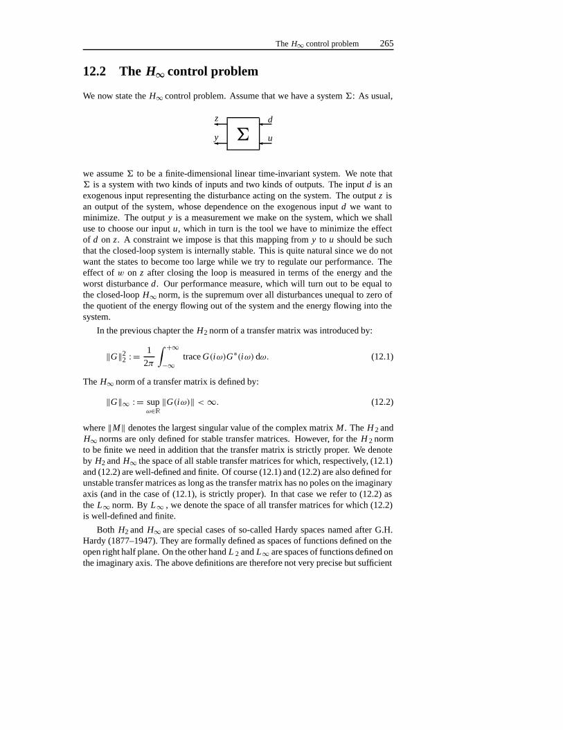
The H∞ control problem 265
12.2 TheH∞ control problem
We now state theH∞ control problem. Assume that we have a system�: As usual,
��y
�
�u
�z d
we assume� to be a finite-dimensional linear time-invariant system. We note that� is a system with two kinds of inputs and two kinds of outputs. The inputd is anexogenous input representing the disturbance acting on the system. The outputz isan output of the system, whose dependence on the exogenous inputd we want tominimize. The outputy is a measurement we make on the system, which we shalluse to choose our inputu, which in turn is the tool we have to minimize the effectof d on z. A constraint we impose is that this mapping fromy to u should be suchthat the closed-loop system is internally stable. This is quite natural since we do notwant the states to become too large while we try to regulate our performance. Theeffect ofw on z after closing the loop is measured in terms of the energy and theworst disturbanced. Our performance measure, which will turn out to be equal tothe closed-loopH∞ norm, is the supremum over all disturbances unequal to zero ofthe quotient of the energy flowing out of the system and the energy flowing into thesystem.
In the previous chapter theH2 norm of a transfer matrix was introduced by:
‖G‖22 : =
1
2π
∫ +∞
−∞traceG(iω)G∗(iω) dω. (12.1)
The H∞ norm of a transfer matrix is defined by:
‖G‖∞ := supω∈R
‖G(iω)‖ <∞. (12.2)
where‖M‖ denotes the largest singular value of the complex matrixM . TheH 2 andH∞ norms are only defined for stable transfer matrices. However, for theH 2 normto be finite we need in addition that the transfer matrix is strictly proper. We denoteby H2 andH∞ the space of all stable transfer matrices for which, respectively, (12.1)and (12.2) are well-defined and finite. Of course (12.1) and (12.2) are also defined forunstable transfer matrices as long as the transfer matrix has no poles on the imaginaryaxis (and in the case of (12.1), is strictly proper). In that case we refer to (12.2) asthe L∞ norm. ByL∞ , we denote the space of all transfer matrices for which (12.2)is well-defined and finite.
Both H2 and H∞ are special cases of so-called Hardy spaces named after G.H.Hardy (1877–1947). They are formally defined as spaces of functions defined on theopen right half plane. On the other handL 2 andL∞ are spaces of functions defined onthe imaginary axis. The above definitions are therefore not very precise but sufficient
266 H∞ control and robustness
for us since we only consider rational transfer matrices in this book. However it isuseful to realize that for stable transfer matrices we have:
‖G‖∞ := sups∈C+
‖G(s)‖ <∞. (12.3)
whereC+ denotes the open right half complex plane.
DefineLn2 as the set of functionsf from [0,∞) to Rn for which
‖ f ‖2 : =(∫ ∞
0‖ f (t)‖2 dt
)1/2
(12.4)
is well-defined and finite, where‖g‖2 : = gTg denotes the Euclidian norm. Thisnorm is induced by the following inner product
〈 f, g〉2 : =∫ ∞
0g(t)T f (t) dt,
In other words‖ f ‖22 = 〈 f, f 〉2. By L2 we denote the set of allf for which ann
exists such thatf ∈ Ln2.
Note that, since we call the extension of theH∞ norm to unstable transfer matri-ces theL∞ norm, it would be natural to call the extension of theH 2 norm to unstabletransfer matrices theL2 norm. We do not do this and, instead, we use the nameL2 norm for the expression (12.4). This is slightly inconsistent. However, the ex-pressions (12.1) and (12.4) are closely related. If we have a function inL 2 then itsLaplace transform will be inH2 and (12.4) for the function will be equal to (12.1)for its Laplace-transform (a consequence of the so-called Parseval’s theorem). It isgood to note that theH2 norm will only be applied to transfer matrices (in the fre-quency domain) while theL 2 norm will only be used for input-output signals (in thetime-domain).
In this book, instead of the above definition, we shall frequently use a time-domain characterization of theH∞ norm. Let� × � be the closed-loop systemobtained by applying a linear controller� to a given system�. If the closed-loopsystem is stable, then the closed-loop transfer matrixG cl is in H∞ . Given the closedloop system, there exists a map which associates to every inputd an outputz, givenzero initial state. We will denote this map, sometimes called theinput-output opera-tor byGcl . It is easy to check thatGcl is a well-defined linear mapping. TheH∞ normof Gcl is equal to theL2 -induced operator norm ofGcl , i.e.
‖Gcl‖∞ = ‖Gcl‖∞ := supd
{ ‖Gcl d‖2
‖d‖2d ∈ L�2, d = 0
}. (12.5)
Note that we will sometimes use the terminologyH∞ norm for an input-output op-eratorG even though it is formally better to call this theL 2 -induced operator norm.
The H∞ control problem 267
In order to see this equality let the closed loop system have impulse responseg.Then we have:
z(t) = (Gcld)(t) =∫ t
0g(t − τ )d(τ ) dτ
If we apply the Laplace transform toz we obtain:
z(s) = Gcl(s)d(s)
where we used the fact that the transfer matrix is equal to the Laplace transform of theimpulse response. On the other hand, Parseval’s theorem, that we already mentionedbefore, tells us:
‖z‖22 =
1
2π
∫ ∞
0z∗(iω)z(iω) dω.
Combining these properties yields:
‖Gcld‖22 =
∫ ∞
0‖Gcl (iω)d(iω)‖2 dω �
(supω‖Gcl(iω)‖2
)‖d‖2
2
= ‖Gcl‖2∞‖d‖22.
Finally, it is not very hard to see that this inequality becomes an equality for thosed that contain only sharp peaks in the direction and at the frequency whereG cl ismaximal. Since we take the supremum over all possibled in (12.5), it is then notdifficult to see that we do get the equality (12.5).
Because of this equality we often refer to theL 2 -induced operator norm of theclosed-loop operatorGcl as theH∞ norm ofGcl . TheH∞ norm of a stable system isdefined as theH∞ norm of the corresponding transfer matrix of that system.
We note that the above alternative interpretation also has the advantage that itgives a natural way to extend theH∞ norm to nonlinear or time-varying systems. Wewill use a finite-horizon version in the next chapter, which is defined as:
‖Gcl‖∞,T : = supd
{ ‖Gcl d‖2,T
‖d‖2,Td ∈ L�2[0, T ], d = 0
}. (12.6)
where
‖ f ‖2,T : =(∫ T
0‖ f (t)‖2 dt
)1/2
<∞,
This is clearly connected to the time-domain interpretation of theH∞ norm givenabove. It is not possible to connect this finite-horizon version to the frequency domaininterpretation (12.2) or (12.1).
TheH∞ norm is motivated as a tool to achieve robustness, i.e. a method to designcontrollers that are insensitive to variations in the model. However, it is very impor-tant to realize that minimizing the closed loopH∞ norm in itself does not have anyconnection with robustness. One can only guarantee robustness in connection withthe small-gain theorem, which will be discussed in the next section.
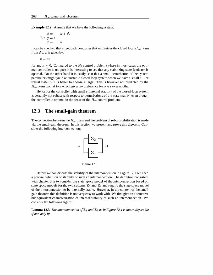
268 H∞ control and robustness
Example 12.2 Assume that we have the following system:
� :x = − u + d,y = x ,z = u.
It can be checked that a feedback controller that minimizes the closed loopH∞ normfrom d to z is given by:
u = εx
for anyε > 0. Compared to theH2 control problem (where in most cases the opti-mal controller is unique), it is interesting to see that any stabilizing state feedback isoptimal. On the other hand it is easily seen that a small perturbation of the systemparameters might yield an unstable closed-loop system when we have a smallε. Forrobust stability it is better to chooseε large. This is however not predicted by theH∞ norm fromd to z which gives no preference for oneε over another.
Hence for the controller with smallε, internal stability of the closed-loop systemis certainly not robust with respect to perturbations of the state matrix, even thoughthe controller is optimal in the sense of theH∞ control problem.
12.3 The small-gain theorem
The connection between theH∞ norm and the problem of robust stabilization is madevia the small-gain theorem. In this section we present and prove this theorem. Con-sider the following interconnection:
�2
�1�
�
z1z2
Figure 12.1
Before we can discuss the stability of the interconnection in Figure 12.1 we needa precise definition of stability of such an interconnection. The definition consistentwith chapter 3 is to consider the state space model of the interconnection based onstate space models for the two systems�1 and�2 and require the state space modelof the interconnection to be internally stable. However, in the context of the smallgain theorem this definition is not very easy to work with. We first give an alternativebut equivalent characterization of internal stability of such an interconnection. Weconsider the following figure:
Lemma 12.3 The interconnection of�1 and�2 as in Figure 12.1 is internally stableif and only if:
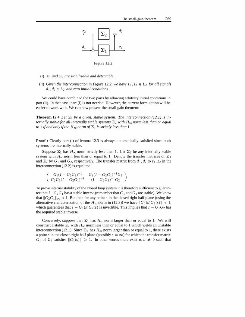
The small-gain theorem 269
� �1
��
��
�2�z2 d2
d1 z1
Figure 12.2
(i) �1 and �2 are stabilizable and detectable.
(ii) Given the interconnection in Figure 12.2, we have z 1, z2 ∈ L2 for all signalsd1, d2 ∈ L2 and zero initial conditions.
We could have combined the two parts by allowing arbitrary initial conditions inpart (ii). In that case, part (i) is not needed. However, the current formulation will beeasier to work with. We can now present the small gain theorem:
Theorem 12.4 Let �1 be a given, stable system. The interconnection (12.1) is in-ternally stable for all internally stable systems �2 with H∞ norm less than or equalto 1 if and only if the H∞ norm of �1 is strictly less than 1.
Proof : Clearly part (i) of lemma 12.3 is always automatically satisfied since bothsystems are internally stable.
Suppose�1 has H∞ norm strictly less than 1. Let�2 be any internally stablesystem withH∞ norm less than or equal to 1. Denote the transfer matrices of�1and�2 by G1 andG2, respectively. The transfer matrix fromd1, d2 to z1, z2 in theinterconnection (12.2) is equal to:(
G1(I − G2G1)−1 G1(I − G2G1)
−1G2
G2G1(I − G2G1)−1 (I − G2G1)
−1G2
)
To prove internal stability of the closed loop system it is therefore sufficient to guaran-tee thatI−G2G1 has a stable inverse (remember thatG 1 andG2 are stable). We knowthat‖G2G1‖∞ < 1. But then for any points in the closed right half plane (using thealternative characterization of theH∞ norm in (12.3)) we have‖G 1(s)G2(s)‖ < 1,which guarantees thatI − G1(s)G2(s) is invertible. This implies thatI − G1G2 hasthe required stable inverse.
Conversely, suppose that�1 has H∞ norm larger than or equal to 1. We willconstruct a stable�2 with H∞ norm less than or equal to 1 which yields an unstableinterconnection (12.1). Since�1 hasH∞ norm larger than or equal to 1, there existsa points in the closed right half plane (possiblys = ∞) for which the transfer matrixG1 of �1 satisfies‖G1(s)‖ � 1. In other words there existu, v = 0 such that
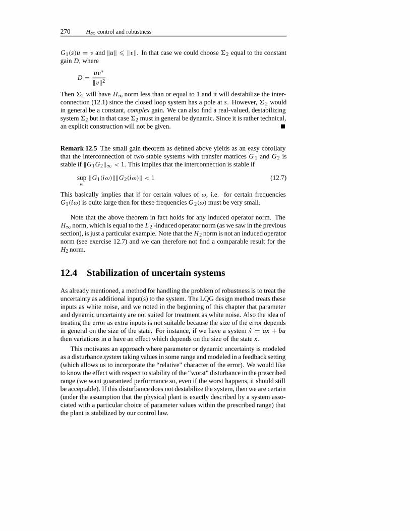
270 H∞ control and robustness
G1(s)u = v and‖u‖ � ‖v‖. In that case we could choose�2 equal to the constantgain D, where
D = uv∗
‖v‖2
Then�2 will have H∞ norm less than or equal to 1 and it will destabilize the inter-connection (12.1) since the closed loop system has a pole ats. However,� 2 wouldin general be a constant,complex gain. We can also find a real-valued, destabilizingsystem�2 but in that case�2 must in general be dynamic. Since it is rather technical,an explicit construction will not be given.
Remark 12.5 The small gain theorem as defined above yields as an easy corollarythat the interconnection of two stable systems with transfer matricesG 1 andG2 isstable if‖G1G2‖∞ < 1. This implies that the interconnection is stable if
supω‖G1(iω)‖‖G2(iω)‖ < 1 (12.7)
This basically implies that if for certain values ofω, i.e. for certain frequenciesG1(iω) is quite large then for these frequenciesG 2(ω)must be very small.
Note that the above theorem in fact holds for any induced operator norm. TheH∞ norm, which is equal to theL 2 -induced operator norm (as we saw in the previoussection), is just a particular example. Note that theH2 norm is not an induced operatornorm (see exercise 12.7) and we can therefore not find a comparable result for theH2 norm.
12.4 Stabilization of uncertain systems
As already mentioned, a method for handling the problem of robustness is to treat theuncertainty as additional input(s) to the system. The LQG design method treats theseinputs as white noise, and we noted in the beginning of this chapter that parameterand dynamic uncertainty are not suited for treatment as white noise. Also the idea oftreating the error as extra inputs is not suitable because the size of the error dependsin general on the size of the state. For instance, if we have a systemx = ax + buthen variations ina have an effect which depends on the size of the statex .
This motivates an approach where parameter or dynamic uncertainty is modeledas a disturbancesystem taking values in some range and modeled in a feedback setting(which allows us to incorporate the “relative" character of the error). We would liketo know the effect with respect to stability of the “worst" disturbance in the prescribedrange (we want guaranteed performance so, even if the worst happens, it should stillbe acceptable). If this disturbance does not destabilize the system, then we are certain(under the assumption that the physical plant is exactly described by a system asso-ciated with a particular choice of parameter values within the prescribed range) thatthe plant is stabilized by our control law.
Stabilization of uncertain systems 271
In a linear setting, parameter uncertainty can very often be modeled as in Figure12.3. Here the system� represents the uncertainty and if the transfer matrix of
�
��
�
�
�
z
y u
d
Figure 12.3
� is zero, then we obtain our nominal model fromu to y. The system� mightcontain uncertain parameters, ignored dynamics after model reduction or discardednon-linearities. The goal is to find a feedback controller that stabilizes the model fora large range of systems�. In this chapter we shall give some examples of differentkinds of uncertainties that can be modeled in the above sense. We shall also showwhat the results of this book, applied to these problems, look like. At this point, weonly show by means of an example that a large class of parameter uncertainties canbe considered as an interconnection of the form depicted in Figure 12.3.
Example 12.6 Assume that we have a single-input, single-output system with twounknown parameters:
�n : x = −ax + bu,y = x .
wherea andb are parameters with values in the ranges[a 0 − ε, a0 + ε] and[b0 −δ, b0+ δ] respectively. We can consider this system as an interconnection of the form(12.3) by choosing the system� to be equal to:
� :x = −a0x + b0u + d,y = x ,
z =(−1
0
)x +
(01
)u.
and the system� to be the following static system:
d = (a − a0 b− b0
)z.
It is easily seen that by scaling we may assume thatε = δ = 1.
On the other hand, if we want to find a controller fromy to u such that the closed-loop system is internally stable for allinternally stable systems� with H∞ norm lessthan or equal toγ , then the problem is equivalent to the following problem: find acontroller which is such that the closed-loop system (if the transfer matrix of� is
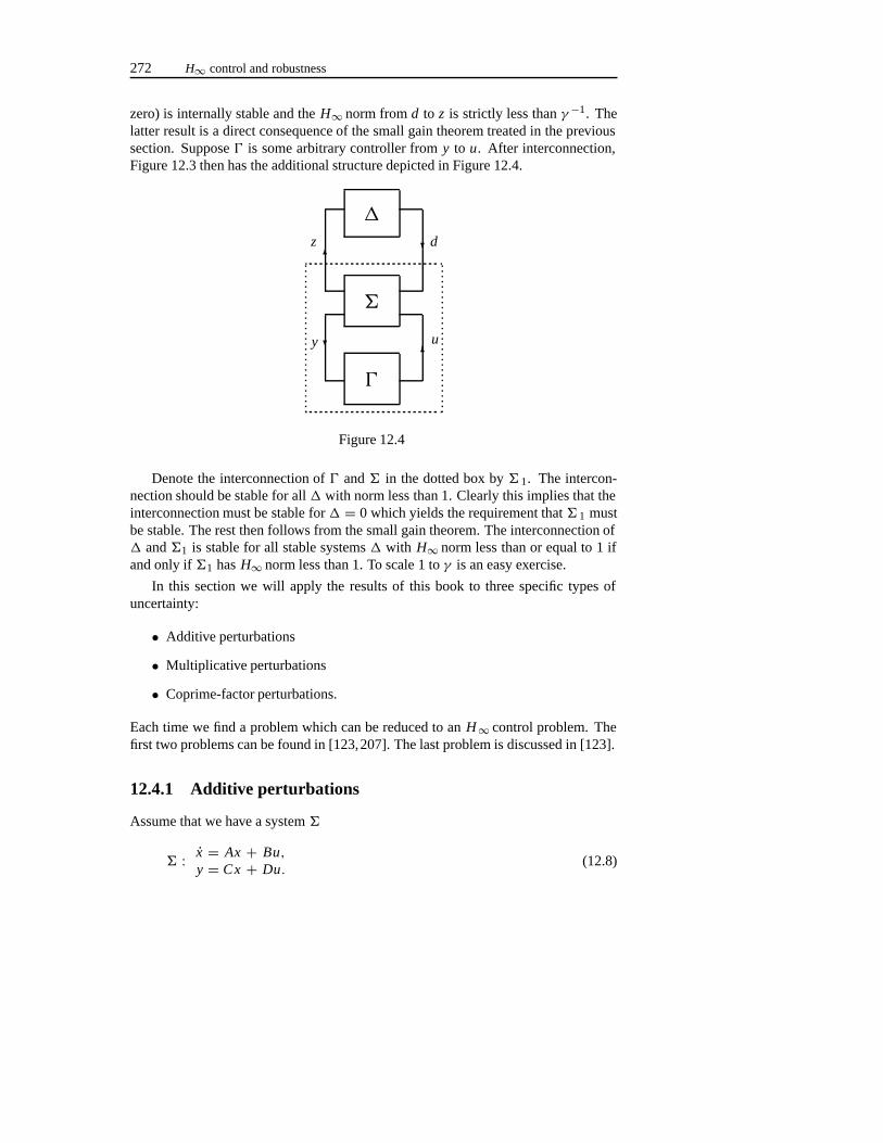
272 H∞ control and robustness
zero) is internally stable and theH∞ norm fromd to z is strictly less thanγ −1. Thelatter result is a direct consequence of the small gain theorem treated in the previoussection. Suppose� is some arbitrary controller fromy to u. After interconnection,Figure 12.3 then has the additional structure depicted in Figure 12.4.
�
�
z d
y u
�
��
��
Figure 12.4
Denote the interconnection of� and� in the dotted box by� 1. The intercon-nection should be stable for all� with norm less than 1. Clearly this implies that theinterconnection must be stable for� = 0 which yields the requirement that� 1 mustbe stable. The rest then follows from the small gain theorem. The interconnection of� and�1 is stable for all stable systems� with H∞ norm less than or equal to 1 ifand only if�1 hasH∞ norm less than 1. To scale 1 toγ is an easy exercise.
In this section we will apply the results of this book to three specific types ofuncertainty:
• Additive perturbations
• Multiplicative perturbations
• Coprime-factor perturbations.
Each time we find a problem which can be reduced to anH∞ control problem. Thefirst two problems can be found in [123,207]. The last problem is discussed in [123].
12.4.1 Additive perturbations
Assume that we have a system�
� : x = Ax + Bu,y = Cx + Du.
(12.8)
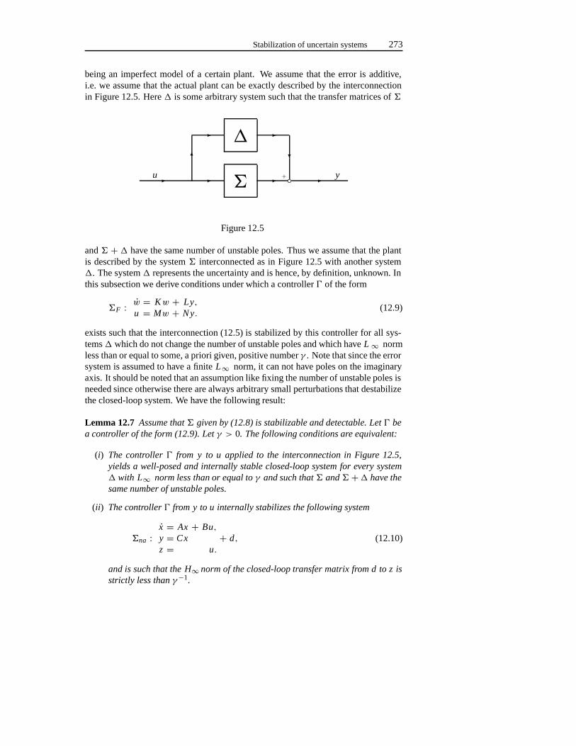
Stabilization of uncertain systems 273
being an imperfect model of a certain plant. We assume that the error is additive,i.e. we assume that the actual plant can be exactly described by the interconnectionin Figure 12.5. Here� is some arbitrary system such that the transfer matrices of�
�
�
� � � �
�
� �
�
u y◦+
Figure 12.5
and� + � have the same number of unstable poles. Thus we assume that the plantis described by the system� interconnected as in Figure 12.5 with another system�. The system� represents the uncertainty and is hence, by definition, unknown. Inthis subsection we derive conditions under which a controller� of the form
�F : w = Kw + Ly,u = Mw + Ny.
(12.9)
exists such that the interconnection (12.5) is stabilized by this controller for all sys-tems� which do not change the number of unstable poles and which haveL ∞ normless than or equal to some, a priori given, positive numberγ . Note that since the errorsystem is assumed to have a finiteL∞ norm, it can not have poles on the imaginaryaxis. It should be noted that an assumption like fixing the number of unstable poles isneeded since otherwise there are always arbitrary small perturbations that destabilizethe closed-loop system. We have the following result:
Lemma 12.7 Assume that � given by (12.8) is stabilizable and detectable. Let � bea controller of the form (12.9). Let γ > 0. The following conditions are equivalent:
(i) The controller � from y to u applied to the interconnection in Figure 12.5,yields a well-posed and internally stable closed-loop system for every system� with L∞ norm less than or equal to γ and such that � and � +� have thesame number of unstable poles.
(ii) The controller � from y to u internally stabilizes the following system
�na :x = Ax + Bu,y = Cx + d,z = u.
(12.10)
and is such that the H∞ norm of the closed-loop transfer matrix from d to z isstrictly less than γ−1.
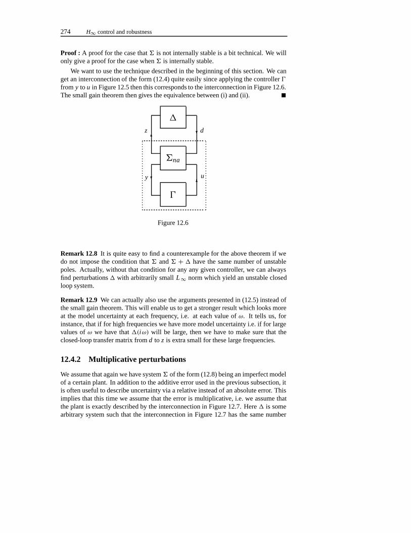
274 H∞ control and robustness
Proof : A proof for the case that� is not internally stable is a bit technical. We willonly give a proof for the case when� is internally stable.
We want to use the technique described in the beginning of this section. We canget an interconnection of the form (12.4) quite easily since applying the controller�
from y to u in Figure 12.5 then this corresponds to the interconnection in Figure 12.6.The small gain theorem then gives the equivalence between (i) and (ii).
�na
�
z d
y u
�
��
��
Figure 12.6
Remark 12.8 It is quite easy to find a counterexample for the above theorem if wedo not impose the condition that� and� + � have the same number of unstablepoles. Actually, without that condition for any any given controller, we can alwaysfind perturbations� with arbitrarily smallL∞ norm which yield an unstable closedloop system.
Remark 12.9 We can actually also use the arguments presented in (12.5) instead ofthe small gain theorem. This will enable us to get a stronger result which looks moreat the model uncertainty at each frequency, i.e. at each value ofω. It tells us, forinstance, that if for high frequencies we have more model uncertainty i.e. if for largevalues ofω we have that�(iω) will be large, then we have to make sure that theclosed-loop transfer matrix fromd to z is extra small for these large frequencies.
12.4.2 Multiplicative perturbations
We assume that again we have system� of the form (12.8) being an imperfect modelof a certain plant. In addition to the additive error used in the previous subsection, itis often useful to describe uncertainty via a relative instead of an absolute error. Thisimplies that this time we assume that the error is multiplicative, i.e. we assume thatthe plant is exactly described by the interconnection in Figure 12.7. Here� is somearbitrary system such that the interconnection in Figure 12.7 has the same number
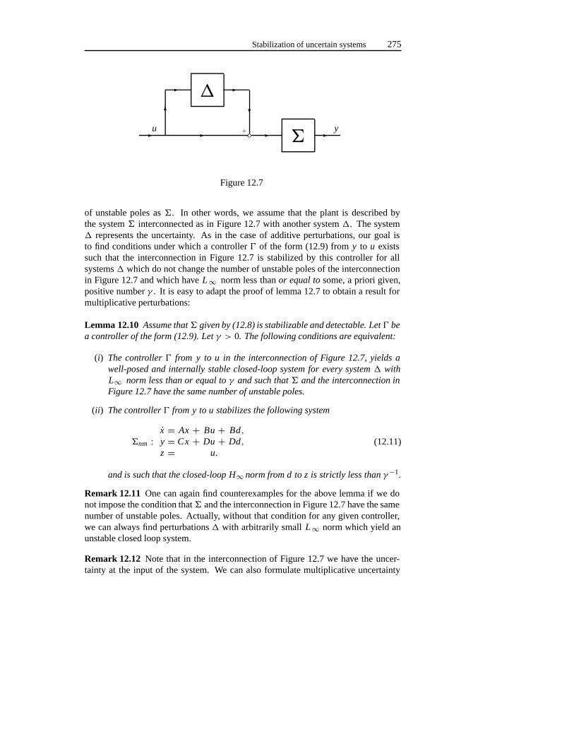
Stabilization of uncertain systems 275
�
�
� � � �
�
� �
�
u y◦+
Figure 12.7
of unstable poles as�. In other words, we assume that the plant is described bythe system� interconnected as in Figure 12.7 with another system�. The system� represents the uncertainty. As in the case of additive perturbations, our goal isto find conditions under which a controller� of the form (12.9) fromy to u existssuch that the interconnection in Figure 12.7 is stabilized by this controller for allsystems� which do not change the number of unstable poles of the interconnectionin Figure 12.7 and which haveL∞ norm less thanor equal to some, a priori given,positive numberγ . It is easy to adapt the proof of lemma 12.7 to obtain a result formultiplicative perturbations:
Lemma 12.10 Assume that� given by (12.8) is stabilizable and detectable. Let � bea controller of the form (12.9). Let γ > 0. The following conditions are equivalent:
(i) The controller � from y to u in the interconnection of Figure 12.7, yields awell-posed and internally stable closed-loop system for every system � withL∞ norm less than or equal to γ and such that � and the interconnection inFigure 12.7 have the same number of unstable poles.
(ii) The controller � from y to u stabilizes the following system
�nm :x = Ax + Bu + Bd,y = Cx + Du + Dd,z = u.
(12.11)
and is such that the closed-loop H∞ norm from d to z is strictly less than γ−1.
Remark 12.11 One can again find counterexamples for the above lemma if we donot impose the condition that� and the interconnection in Figure 12.7 have the samenumber of unstable poles. Actually, without that condition for any given controller,we can always find perturbations� with arbitrarily smallL∞ norm which yield anunstable closed loop system.
Remark 12.12 Note that in the interconnection of Figure 12.7 we have the uncer-tainty at the input of the system. We can also formulate multiplicative uncertainty
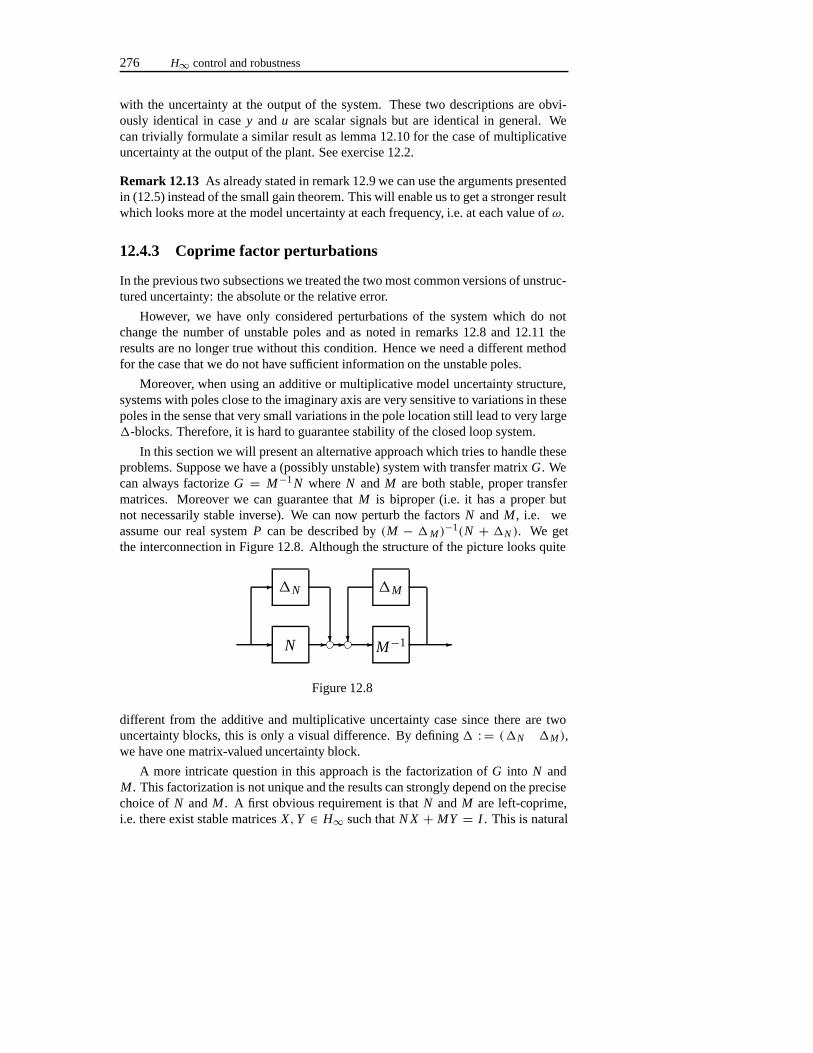
276 H∞ control and robustness
with the uncertainty at the output of the system. These two descriptions are obvi-ously identical in casey andu are scalar signals but are identical in general. Wecan trivially formulate a similar result as lemma 12.10 for the case of multiplicativeuncertainty at the output of the plant. See exercise 12.2.
Remark 12.13 As already stated in remark 12.9 we can use the arguments presentedin (12.5) instead of the small gain theorem. This will enable us to get a stronger resultwhich looks more at the model uncertainty at each frequency, i.e. at each value ofω.
12.4.3 Coprime factor perturbations
In the previous two subsections we treated the two most common versions of unstruc-tured uncertainty: the absolute or the relative error.
However, we have only considered perturbations of the system which do notchange the number of unstable poles and as noted in remarks 12.8 and 12.11 theresults are no longer true without this condition. Hence we need a different methodfor the case that we do not have sufficient information on the unstable poles.
Moreover, when using an additive or multiplicative model uncertainty structure,systems with poles close to the imaginary axis are very sensitive to variations in thesepoles in the sense that very small variations in the pole location still lead to very large�-blocks. Therefore, it is hard to guarantee stability of the closed loop system.
In this section we will present an alternative approach which tries to handle theseproblems. Suppose we have a (possibly unstable) system with transfer matrixG. Wecan always factorizeG = M−1N whereN and M are both stable, proper transfermatrices. Moreover we can guarantee thatM is biproper (i.e. it has a proper butnot necessarily stable inverse). We can now perturb the factorsN and M , i.e. weassume our real systemP can be described by(M − �M )
−1(N + �N ). We getthe interconnection in Figure 12.8. Although the structure of the picture looks quite
N
�N
M−1
�M
�
�
�� ��� �
Figure 12.8
different from the additive and multiplicative uncertainty case since there are twouncertainty blocks, this is only a visual difference. By defining� : = (�N �M ),we have one matrix-valued uncertainty block.
A more intricate question in this approach is the factorization ofG into N andM . This factorization is not unique and the results can strongly depend on the precisechoice ofN andM . A first obvious requirement is thatN andM are left-coprime,i.e. there exist stable matricesX,Y ∈ H∞ such thatN X + MY = I . This is natural
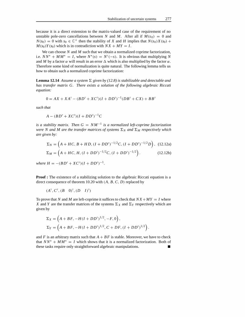
Stabilization of uncertain systems 277
because it is a direct extension to the matrix-valued case of the requirement of nounstable pole-zero cancellations betweenN and M . After all if M(s0) = 0 andN(s0) = 0 with s0 ∈ C+ then the stability ofX and H implies thatN(s0)X (s0) +M(s0)Y (s0) which is in contradiction withN X + MY = I .
We can chooseN andM such that we obtain a normalized coprime factorization,i.e. N N∗ + M M∗ = I , whereN∗(s) = NT(−s). It is obvious that multiplyingNandM by a factorα will result in an error� which is also multiplied by the factorα.Therefore some kind of normalization is quite natural. The following lemma tells ushow to obtain such a normalized coprime factorization:
Lemma 12.14 Assume a system � given by (12.8) is stabilizable and detectable andhas transfer matrix G. There exists a solution of the following algebraic Riccatiequation:
0= AX + X AT − (B DT + XCT)(I + DDT)−1(DBT + C X) + B BT
such that
A − (B DT + XCT)(I + DDT)−1C
is a stability matrix. Then G = N M−1 is a normalized left-coprime factorizationwere N and M are the transfer matrices of systems �N and �M respectively whichare given by:
�N =(
A + H C, B + H D, (I + DDT)−1/2C, (I + DDT)−1/2D), (12.12a)
�M =(
A + H C, H, (I + DDT)−1/2C, (I + DDT)−1/2). (12.12b)
where H = −(B DT + XCT)(I + DDT)−1.
Proof : The existence of a stabilizing solution to the algebraic Riccati equation is adirect consequence of theorem 10.20 with(A, B,C, D) replaced by
(AT,CT, (B 0)T, (D I )T)
To prove thatN andM are left-coprime it suffices to check thatN X+MY = I whereX andY are the transfer matrices of the systems�X and�Y respectively which aregiven by
�X =(
A + B F,−H (I + DDT)1/2,−F,0),
�Y =(
A + B F,−H (I + DDT)1/2,C + DF, (I + DDT)1/2).
andF is an arbitrary matrix such thatA+ B F is stable. Moreover, we have to checkthat N N∗ + M M∗ = I which shows that it is a normalized factorization. Both ofthese tasks require only straightforward algebraic manipulations.
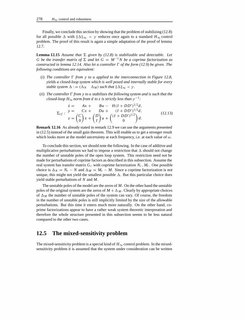
278 H∞ control and robustness
Finally, we conclude this section by showing that the problem of stabilizing (12.8)for all possible� with ‖�‖∞ < γ reduces once again to a standardH∞ controlproblem. The proof of this result is again a simple adaptation of the proof of lemma12.7.
Lemma 12.15 Assume that � given by (12.8) is stabilizable and detectable. LetG be the transfer matrix of � and let G = M−1N be a coprime factorization asconstructed in lemma 12.14. Also let a controller � of the form (12.9) be given. Thefollowing conditions are equivalent:
(i) The controller � from y to u applied to the interconnection in Figure 12.8,yields a closed-loop system which is well posed and internally stable for everystable system � : = (�N �M ) such that ‖�‖∞ < γ .
(ii) The controller � from y to u stabilizes the following system and is such that theclosed-loop H∞ norm from d to z is strictly less than γ−1:
�c f :x = Ax + Bu − H (I + DDT)1/2d,y = Cx + Du + (I + DDT)1/2d,
z =(
C0
)x +
(DI
)u +
((I + DDT)1/2
0
)d.
(12.13)
Remark 12.16 As already stated in remark 12.9 we can use the arguments presentedin (12.5) instead of the small gain theorem. This will enable us to get a stronger resultwhich looks more at the model uncertainty at each frequency, i.e. at each value ofω.
To conclude this section, we should note the following. In the case of additive andmultiplicative perturbations we had to impose a restriction that� should not changethe number of unstable poles of the open loop system. This restriction need not bemade for perturbations of coprime factors as described in this subsection. Assume thereal system has transfer matrixGr with coprime factorizationNr ,Mr . One possiblechoice is�N = Nr − N and�M = Mr − M . Since a coprime factorization is notunique, this might not yield the smallest possible�. But this particular choice doesyield stable perturbations ofN andM .
The unstable poles of the model are the zeros ofM . On the other hand the unstablepoles of the original system are the zeros ofM+�M . Clearly by appropriate choicesof �M the number of unstable poles of the system can vary. Of course, the freedomin the number of unstable poles is still implicitly limited by the size of the allowableperturbations. But this time it enters much more naturally. On the other hand, co-prime factorizations appear to have a rather weak system theoretic interpreation andtherefore the whole structure presented in this subsection seems to be less naturalcompared to the other two cases.
12.5 The mixed-sensitivity problem
The mixed-sensitivity problem is a special kind ofH∞ control problem. In the mixed-sensitivity problem it is assumed that the system under consideration can be written
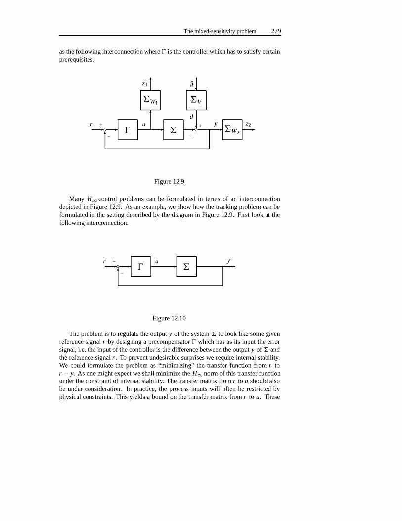
The mixed-sensitivity problem 279
as the following interconnection where� is the controller which has to satisfy certainprerequisites.
�
�W1
�
�V
�W2� �
��
�
�
�
�
� � �
z1 d
dyur z2+
− +
+◦ ◦
Figure 12.9
Many H∞ control problems can be formulated in terms of an interconnectiondepicted in Figure 12.9. As an example, we show how the tracking problem can beformulated in the setting described by the diagram in Figure 12.9. First look at thefollowing interconnection:
� �� ��
� �yur +
−◦
Figure 12.10
The problem is to regulate the outputy of the system� to look like some givenreference signalr by designing a precompensator� which has as its input the errorsignal, i.e. the input of the controller is the difference between the outputy of � andthe reference signalr . To prevent undesirable surprises we require internal stability.We could formulate the problem as “minimizing" the transfer function fromr tor − y. As one might expect we shall minimize theH∞ norm of this transfer functionunder the constraint of internal stability. The transfer matrix fromr to u should alsobe under consideration. In practice, the process inputs will often be restricted byphysical constraints. This yields a bound on the transfer matrix fromr to u. These
280 H∞ control and robustness
transfer matrices fromr to r − y and fromr to u are given by:
S : = (I + G H )−1 ,
T : = H (I + G H )−1 ,
respectively, whereG and H denote the transfer matrices of� and�. Here S iscalled thesensitivity function andT is called thecontrol sensitivity function. A smallfunction S expresses good tracking properties while a small functionT expressessmall inputsu. Note thatS + GT = I and therefore there is a trade-off: makingS smaller will in general makeT larger. We add a signald to the outputy as inFigure 12.9 on the preceding page. Then the transfer matrix fromd to y is equal tothe sensitivity matrixS and the transfer matrix fromd to u is equal to the controlsensitivity matrixT .
Although we assume the tracking signal to be, a priori, unknown, in most caseswe know that our tracking signal will have a limited frequency spectrum, i.e. theFourier transform of the reference signalr will be small for many frequencies, i.e.‖r(iω)‖ is small for many values ofω. In most cases, we only track slowly varyingsignals which implies that‖r (iω)‖ is small for large frequenciesω. By minimizing‖W2S‖∞, whereW2 is large for small values ofω and small for large values ofω,we actually put more effort in achieving good tracking for small values ofω. In otherwords, we put most effort in tracking slowly time-varying signalsr .
On the other hand it is in general very difficult to implement an inputu whichvaries very quickly. Therefore we want to ensure in particular thatT is small forlarge frequencies. By minimizing‖W1T ‖∞, whereW1 is small for small values ofω and large for large values ofω, we actually put more emphasis on avoiding fastchanges over time in the inputu.
The transfer matricesW1 andW2 are referred to as weighting functions to expressthe above information. It helps us to incorporate our requirements that we wantSto be small at low frequencies andT to be small at high frequencies. Note that itis general impossible to makeS andT both small for the same frequency becauseS + GT = I . It is obvious that if we want track signals up to higher frequencies, i.ewith faster time-variations, yet have severe bandwidth limitations on the controller,i.e. the controller can not vary very fast over time then we will not be able to obtainsatisfactory results.
Therefore, in Figure 12.9 on the preceding page, the systems�W1, �W2 and�V
are weights which are chosen in such a way that we put more effort in regulatingfrequencies of interest instead of one uniform bound. To handle the above conflictingrequirements the choice of these weights is the crucial component in the design.
In the above, we have given a sketch of the ideas resulting in the structure of theinterconnection depicted in the interconnection (12.9). Note that the transfer matrixfrom the disturbanced to z1 andz2 is(
W1T VW2SV
)(12.14)
whereW1, W2 andV are the transfer matrices of�W1, �W2 and�V , respectively.
The bounded real lemma 281
Note that we can also use these weights to stress the relative importance of minimiz-ing the sensitivity matrixS with respect to the importance of minimizing the controlsensitivity matrixT by multiplyingW1 by a scalar.
We want to find a controller which minimizes theH∞ norm of the transfer matrix(12.14) and which yields internal stability. This problem can be solved using thetechniques we present in this book.
12.6 The bounded real lemma
As we have shown in the previous sections, theH∞ norm can be used as a tool inthe study of multivariable control systems. In the next two chapters we will study theminimization of theH∞ norm using stabilizing controllers. In the present section, wewill establish methods to determine theH∞ norm of a system�:
x = Ax + Ed,z = Cx + Dd.
(12.15)
We note that the time-domain interpretation of theH∞ norm as theL2 -induced op-erator norm suggests to study the following problem:
supd∈L2
{‖z‖2
2 − γ 2‖d‖22 | x(0) = ξ
}. (12.16)
If the system has initial state 0, i.e.ξ = 0 then this expression is finite only if theH∞ norm of the system is less than or equal toγ . After all if we use the expression(12.5) for theH∞ norm then we see that if theH∞ norm is larger thanγ then thereexists a signald ∈ L2 such that
‖z‖2
‖d‖2
> γ
but taking the square and then multiplying with‖d‖22 we obtain:
‖z‖22− γ 2‖d‖2
2 =: r > 0. (12.17)
If we replaced by αd then the resulting output is equal toαz because the initialstate is zero. But then the resulting cost is equal toα2r . Sincer > 0 we see thatby choosing large enoughα we can make the cost function arbitrary large and thesupremum will hence not be finite.
This problem is closely related to the linear quadratic regulator problem and wewill solve this problem using similar techniques. As a matter of fact, it is an exampleof a so-called indefinite linear quadratic regulator problem. If we rewrite our objectiveas maximizing:∫ ∞
0x(t)TCTCx(t)+x(t)TCT Dd(t)+d(t)T DTCx(t)+d(t)T
(DT D − γ 2I
)d(t) dt
282 H∞ control and robustness
or equivalently of minimizing:∫ ∞
0−x(t)TCTCx(t)−x(t)TCT Dd(t)−d(t)T DTCx(t)+d(t)T
(γ 2I − DT D
)d(t) dt
then the connection to the theory of chapter 10 should be obvious. However, thequadratic term inx(t) is negative semi-definite and hence the resulting cost couldactually be negative and this does yield some crucial differences compared to theresults presented in chapter 10.
We first study the finite horizon version and then take the limit as time tends toinfinity. This will be done in the following two subsections.
12.6.1 A finite horizon
Consider the system (12.15). We first note that if theL 2 [0, T ]-induced operator normof this system is smaller than some boundγ > 0 then we must have‖D‖ < γ .
Lemma 12.17 Consider the system (12.15). If the L 2 [0, T ]-induced operator normis smaller than some bound γ > 0 then ‖D‖ < γ .
Proof : We prove this by contradiction. Assume‖D‖ � γ . Then there exists a vectord0 such that‖Dd0‖ � γ ‖d0‖. We then apply a disturbancedof the form:
d(t) ={ε−1/2d0 0< t < ε,
0 elsewhere,
to the system (12.15), and it can be easily seen that:
limε→0
‖zε‖2,T = ‖Dd0‖ � γ ‖d0‖ = γ ‖dε‖2,T
(the last equality holds for allε). Using (12.5) we then immediately find that theH∞ norm of the system (12.15) is larger thanγ . This yields the required contradic-tion.
If the L2 [0, T ]-induced operator norm is smaller than some boundγ > 0 then
supd
{‖z‖2
2,T − γ 2‖d‖22,T
}� 0 (12.18)
for initial conditionx(0) = 0. Assume there exists ad ∈ L 2 [0, T ] such that (12.18)is positive. Then there existsde ∈ L2 defined by:
de(t) ={
d(t) t � T
0 t > T
The bounded real lemma 283
such that
‖z‖22− γ 2‖d‖2
2 � ‖z‖22,T − γ 2‖d‖2
2 = ‖z‖22,T − γ 2‖d‖2
2,T > 0.
But this inputd and the resulting outputz then yield a contradiction that theH∞ normis less thanγ by using the characterization (12.5) for theH∞ norm.
It will turn later that the use of non-zero initial state will help us in the proof ofour main result. We have the following lemma:
Lemma 12.18 Let system (12.15) be given. Then
supd∈L2
{ ‖z‖22,T − γ 2‖d‖2
2,T x(0) = ξ }(12.19)
is finite for all ξ ∈ Rn if the L2 [0, T ]-induced operator norm is strictly less than γ .
Proof : Suppose theL 2 [0, T ]-induced operator norm is strictly less thanγ , sayδ.Then we find:
‖z‖22,T − γ 2‖d‖2
2,T = ‖z0,d + zξ,0‖22,T − γ 2‖d‖2
2,T
� ‖z0,d‖22,T + ‖zξ,0‖2
2,T + 2‖z0,d‖2,T · ‖zξ,0‖2,T − γ 2‖d‖22,T
� (δ2− γ 2)‖d‖22,T + 2δ‖zξ,0‖2,T · ‖d‖2,T + ‖zξ,0‖2
2,T
� supα∈[0,∞)
(δ2− γ 2)α2 + 2δ‖zξ,0‖2,T · α + ‖zξ,0‖22,T,
<∞wherez0,d denotes the output of the system with disturbanced and zero initial statewhile zξ,0 denotes the output of the system with disturbance 0 and initial statex(0) =ξ . The last inequality is a consequence of the fact thatδ < γ . This proves that (12.19)is finite for all ξ ∈ Rn.
We define
C(d, ξ, τ ) : =∫ T
τ
zT(t)z(t) − γ 2dT(t)d(t) dt
wherez is the output of the system with inputd and initial statex(τ ) = ξ . We willinvestigate in detail the following criterion:
C∗(ξ, τ ) : = supd
C(d, ξ, τ ) (12.20)
for arbitrary initial statex(τ ) = ξ , and where we maximize overd ∈ L 2 [τ, T ].Lemma 12.18 guarantees thatC ∗(ξ,0) is bounded from above. Moreover, ford = 0,we haveC(0, ξ,0) � 0 and henceC ∗(ξ,0) is also bounded from below. We get thatif the L2 [0, T ]-induced operator norm is less thanγ thenC ∗(ξ,0) is bounded.
284 H∞ control and robustness
Next we claim thatC∗(ξ, τ ) is an non-increasing function ofτ . This is a conse-quence of the following arguments, whereτ1 � τ2.
C∗(ξ, τ1) : = supd
C(d, ξ, τ1)
= supd
∫ T
τ1
‖z(t)‖2 − γ 2‖d(t)‖2 dt
� supd
{∫ τ
τ1
‖z(t)‖2 − γ 2‖d(t)‖2 dt
+∫ T
τ
‖z(t)‖2 dt
∣∣∣∣ d(t) = 0, t > T
}
� supd
infu
∫ τ
τ1
‖z(t)‖2 − γ 2‖d(t)‖2 dt
= C∗(ξ, τ2)
whereτ = T − τ2 + τ1 and where, in the last step, we use that the system is time-invariant.
Hence we note that, ifC∗(ξ,0) is bounded, thenC ∗(ξ, τ ) is bounded for allτ ∈[0, T ]. We will use theorem 10.7. We apply this theorem, with time reversed, to thefollowing Riccati differential equation:
−P = AT P+P A+CTC+(P E + CT D
) (γ 2I − DT D
)−1 (ET P + DTC
)(12.21)
Note that we already concluded that‖D‖ must be less thanγ , and therefore theinverse is well-defined. We know there existsT1 � 0 such that this Riccati equationhas a solutionP on the interval[T1, T ] with P(T ) = 0. If we show that this solutionis uniformly bounded on the interval[T1, T ] with a bound independent ofT1 thentheorem 10.7 guarantees that a solutionP exists on the whole interval[0, T ]. Thebound onP is a consequence of the following lemma.
Lemma 12.19 Assume the Riccati equation (12.21) has a solution P with P(T ) = 0on the interval [T1, T ]. Then we have:
C∗(ξ, τ ) = ξ T P(τ )ξ
for all ξ ∈ Rn and all τ ∈ [T1, T ].
Proof : We will use acompletion of the squares argument similar to the one used inchapter 10. We get
C∗(ξ, τ ) : = supd
C(d, ξ, τ )
: = ξ T P(τ )ξ + supd
∫ T
τ
‖z(t)‖2 − γ 2‖d(t)‖2
+(
d
dtx T(t)P(t)x(t)
)dt
The bounded real lemma 285
= ξ T P(τ )ξ + supd−‖(γ 2I − DT D)1/2(d − Fx)‖2
2,T
whereF(t) = (γ 2I − DT D)−1(ET P(t) + DTC). It is obvious that the maximizingd is given byd = Fx .
We have shown that, if theL 2 [0, T ]-induced operator norm is less thanγ , then‖D‖ < γ andC∗(ξ,0) is bounded for allξ ∈ Rn and, moreover, we have shown thatC∗(ξ,0) � C∗(ξ, τ ) for all τ ∈ [0, T ]. Therefore, the above lemma shows thatP isuniformly bounded. But we already discussed before lemma 12.19 that this impliesthat a solutionP of the Riccati equation (12.21) exists on the complete interval[0, T ].
We will prove the converse. Assume that‖D‖ < γ and there exists a solutionP of the Riccati equation (12.21) withP(T ) = 0. We show that this implies thatthe L2 [0, T ]-induced operator norm is strictly less thanγ . If we use the comple-tion of the squares argument from the proof of lemma (12.19) then, for zero initialconditions, we obtain:
‖z‖22,T − γ 2‖d‖2
2,T = −‖(γ 2I − DT D)1/2(d − Fx)‖22,T � 0
for all d ∈ L2 [0, T ]. This immediately implies that theL 2 [0, T ]-induced operatornorm is less than or equal toγ . We still have to prove that the norm is strictly lessthanγ . Introduce a new variablev = (γ 2I − DT D)1/2(d − Fx) and consider thefollowing system
�vd : x = (A + E F)x + E(γ 2I − DT D)−1/2v,
d = Fx + (γ 2I − DT D)−1/2v.
This system defines an operatorGvd mappingv to d, which has a finiteL 2 [0, T ]-induced operator norm. Then we get
‖z‖22,T − γ 2‖d‖2
2,T = −γ 2‖v‖22,T � −γ 2‖Gvd‖−2∞,T‖d‖2
2,T
which guarantees that theL 2 [0, T ]-induced operator norm is less than or equal to
γ
√1− ‖Gvd‖−2∞,T < γ.
Thus, we have proven the following lemma:
Lemma 12.20 Let the system � be given by (12.15). Then the L 2 [0, T ]-inducedoperator norm of � is less than γ if and only if ‖D‖ < γ and there exists a solutionP of (12.21) with P(T ) = 0.
Note that from the proof it can be seen that the above lemma is also valid fortime-varying systems (where we need to require that‖D(t)‖ < γ for all t ∈ [0, T ]).However, in the next subsection we study the infinite horizon case where our approachwill depend on the fact that the system is time-invariant.
286 H∞ control and robustness
12.6.2 Infinite horizon
We again consider the system (12.15). We will basically apply the limit asT → ∞to lemma 12.20. Assume the system is internally stable, and hasH∞ norm less thanγ . Then, similarly as in lemma 12.18, we can show that:
C∗(ξ) : = supd
∫ ∞
0zT(t)z(t)− γ 2dT(t)d(t) dt (12.22)
is bounded for all initial conditionsx(0) = ξ . We find:
C∗(0) : = supd∈L2 [0,∞)
∫ ∞
0‖z(t)‖2 − γ 2‖d(t)‖2 dt
� supd∈L2 [0,∞)
{ ∫ ∞
0‖z(t)‖2 dt
−γ 2∫ T
0‖d(t)‖2 dt
∣∣∣∣ d(t) = 0, t > T
}
� supd∈L2 [0,T ]
∫ T
0‖z(t)‖2 − γ 2‖d(t)‖2 dt . (12.23)
This shows that theL2 [0, T ]-induced operator norm is less than or equal to theH∞ norm for allT . Consider the following Riccati differential equation:
Q = AT Q + Q A + CTC + (QE + CT D
) (γ 2I − DT D
)−1 (ET Q + DTC
),
with Q(0) = 0. We haveQ(t) = P(T − t) whenP satisfies (12.21) withP(T ) = 0.We also know that theL2 [0, T ]-induced operator norm is less than theH∞ normand hence less thanγ for all T . Therefore, the results of the previous subsectionimply that a solutionQ exists for all t . MoreoverQ is increasing and bounded.This obviously implies that a limitQ exists, which must satisfy the algebraic Riccatiequation:
0= AT Q+ Q A+CTC+(QE + CT D
) (γ 2I − DT D
)−1 (ET Q + DTC
). (12.24)
We need an additional condition onQ for which we need to do some work. We knowthat theH∞ norm fromd to z is less thanγ , sayδ. But then, for allT > 0, theL2 [0, T ]-induced operator norm is less than or equal toδ. We obtain:
‖z‖22,T − γ 2‖d‖2
2,T = ‖z0,d + zξ,0‖22,T − γ 2‖d‖2
2,T
� ‖z0,d‖22,T + ‖zξ,0‖2
2,T + 2‖z0,d‖2,T · ‖zξ,0‖2,T − γ 2‖d‖22,T
� ‖z0,d‖22,T + ‖zξ,0‖2
2+ 2‖z0,d‖2,T · ‖zξ,0‖2− γ 2‖d‖22,T
� (δ2− γ 2)‖d‖22,T + ‖zξ,0‖2
2+ 2δ‖d‖22,T · ‖zξ,0‖2
� (γ 2− δ2)(
c2− (‖d‖2,T − c1)2)
The bounded real lemma 287
for certain constantsc1 andc2, independent ofT . Choose an arbitraryT . We notethat fordT = FTx with FT(t) = (γ 2I − DT D)−1(ET Q(T − t)+ DTC) we have
‖z‖22,T − γ 2‖dT‖2
2,T = ξ T Q(T − t)ξ � 0
for all initial conditionsx(0) = ξ and hence
(‖dT‖2,T − c1)2 � c2.
This implies that‖dT‖2,T < α, with α independent ofT . It is trivial to see that‖dT‖2,T1
< ‖dT‖2,T < α for all T � T1. Finally, FT(t) → F (T → ∞) for all t ,whereF = (γ 2I − DT D)−1(ET Q + DTC), and thereforedT(t)→ d(t) asT →∞for all t , whered = Fx . But then
‖d‖2,T1= lim
T→∞ ‖dT‖2,T1< α
for all T1, which guarantees thatd ∈ L 2 . On the other hand,d is determined by
x = Ax + Ed = (A + E F)x .
SinceA is a stability matrix andEd ∈ L 2 we havex ∈ L2 for all initial states (seeexercise 13.1). This implies that
A + E F = A + E(γ 2I − DT D)−1(ET Q + DTC) (12.25)
is asymptotically stable. Finally, it is obvious thatQ � 0.
We will now show the converse. Assume there exists a matrixQ � 0 whichsatisfies (12.24) and is such that (12.25) is stable. First, we will check whether thesystem is stable. Assumex = 0 is an eigenvector ofA with eigenvalueλ. From(12.24) we obtain:
2(�eλ)x∗ Qx = −‖(γ 2I − DT D)−1/2(ET Q + DTC)x‖2− ‖Cx‖2.
Suppose�eλ � 0. Then the above equation implies that we must have(E T Q +DTC)x = 0. This implies(A + E F)x = λx which yields a contradiction sinceA + E F is a stability matrix. Therefore,A must be a stability matrix.
It is also easy to check that we have:
‖z‖22,T − γ 2‖d‖2
2,T = −‖(γ 2I − DT D)1/2(d − Fx)‖22,T − x T(T )Qx(T ).
Since the system is stable, andd ∈ L2 , we havez ∈ L2 andx(T )→ 0 asT →∞.Thus we get:
‖z‖22− γ 2‖d‖2
2 = −∫ ∞
0[d(t)− Fx(t)]T
(γ 2I − DT D
)[d(t)− Fx(t)] dt
for initial statex(0) = 0. Define a new variablev by puttingv = (γ 2I−DT D)1/2(d−Fx) and consider the system:
�vd : x = (A + E F)x − E(γ 2I − DT D)−1/2v
d = Fx − (γ 2I − DT D)−1/2v
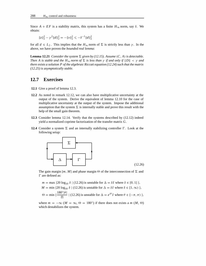
288 H∞ control and robustness
Since A + E F is a stability matrix, this system has a finiteH∞ norm, sayδ. Weobtain:
‖z‖22− γ 2‖d‖2
2 = −‖v‖22 � −δ−1‖d‖2
2
for all d ∈ L2 . This implies that theH∞ norm of� is strictly less thanγ . In theabove, we have proven thebounded real lemma:
Lemma 12.21 Consider the system� given by (12.15). Assume (C, A) is detectable.Then A is stable and the H∞ norm of � is less than γ if and only if ‖D‖ < γ andthere exists a solution P of the algebraic Riccati equation (12.24) such that the matrix(12.25) is asymptotically stable.
12.7 Exercises
12.1 Give a proof of lemma 12.3.
12.2 As noted in remark 12.12, we can also have multiplicative uncertainty at theoutput of the system. Derive the equivalent of lemma 12.10 for the case ofmultiplicative uncertainty at the output of the system. Impose the additionalassumption that the system� is internally stable and prove this result with thehelp of the small gain theorem.
12.3 Consider lemma 12.14. Verify that the systems described by (12.12) indeedyield a normalized coprime factorization of the transfer matrixG.
12.4 Consider a system� and an internally stabilizing controller�. Look at thefollowing setup:
�
� �
�
� �
�
�
(12.26)
The gain margin[m,M] and phase margin� of the interconnection of� and� are defined as:
m = max{20 log10 δ | (12.26) is unstable for� = δ I whereδ ∈ [0,1] },M = min {20 log10 δ | (12.26) is unstable for� = δ I whereδ ∈ [1,∞) },� = min {180◦|θ |
| (12.26) is unstable for� = eiθ I whereθ ∈ [−π, π) },
wherem = −∞ (M = ∞, � = 180◦) if there does not exists am (M , �)which destabilizes the system.
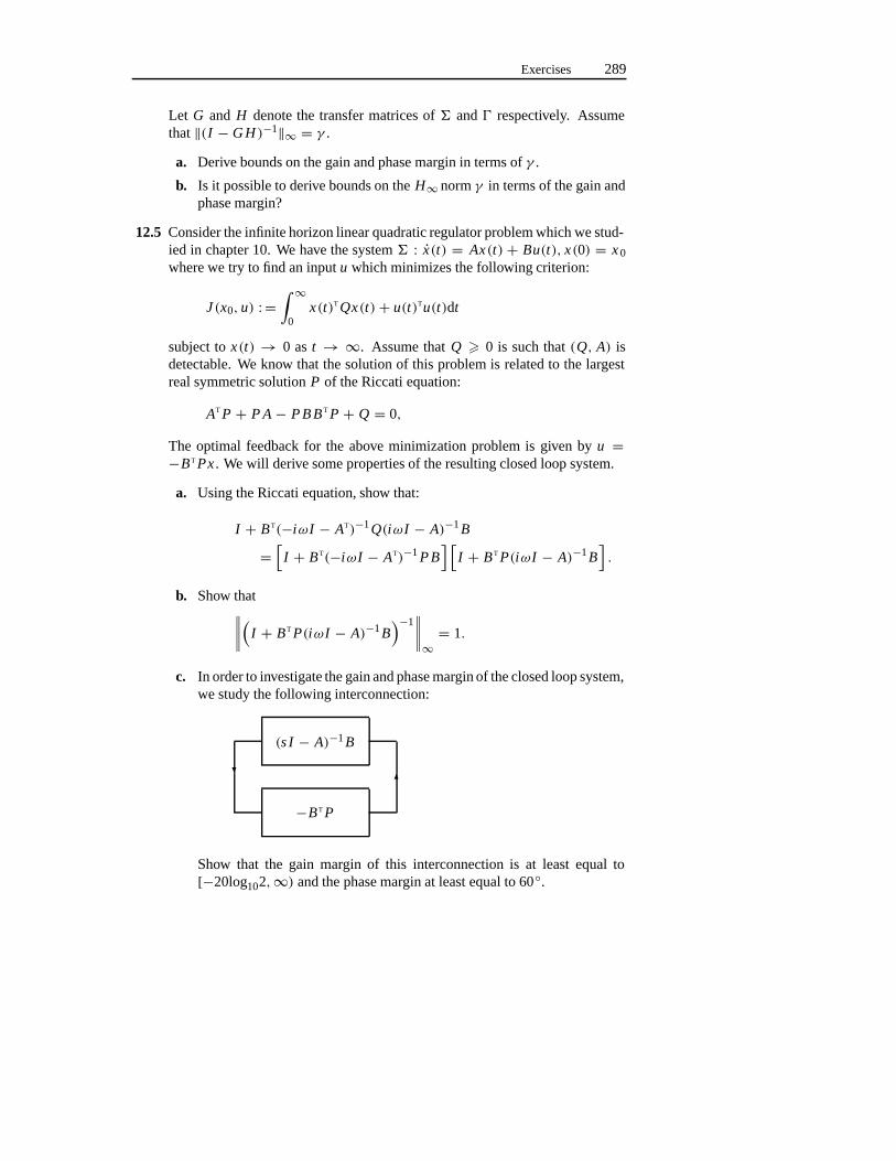
Exercises 289
Let G and H denote the transfer matrices of� and� respectively. Assumethat‖(I − G H )−1‖∞ = γ .
a. Derive bounds on the gain and phase margin in terms ofγ .
b. Is it possible to derive bounds on theH∞ normγ in terms of the gain andphase margin?
12.5 Consider the infinite horizon linear quadratic regulator problem which we stud-ied in chapter 10. We have the system� : x(t) = Ax(t) + Bu(t), x(0) = x 0where we try to find an inputu which minimizes the following criterion:
J (x0, u) : =∫ ∞
0x(t)T Qx(t)+ u(t)Tu(t)dt
subject tox(t) → 0 ast → ∞. Assume thatQ � 0 is such that(Q, A) isdetectable. We know that the solution of this problem is related to the largestreal symmetric solutionP of the Riccati equation:
AT P + P A − P B B T P + Q = 0,
The optimal feedback for the above minimization problem is given byu =−BT Px . We will derive some properties of the resulting closed loop system.
a. Using the Riccati equation, show that:
I + BT(−iωI − AT)−1Q(iωI − A)−1B
=[
I + BT(−iωI − AT)−1P B] [
I + BT P(iωI − A)−1B].
b. Show that∥∥∥∥(I + BT P(iωI − A)−1B)−1
∥∥∥∥∞ = 1.
c. In order to investigate the gain and phase margin of the closed loop system,we study the following interconnection:
��
−BT P
(s I − A)−1B
Show that the gain margin of this interconnection is at least equal to[−20log102,∞) and the phase margin at least equal to 60◦.
290 H∞ control and robustness
12.6 Consider the following system:
� :
(x1x2
)=
(1 10 1
)(x1x2
)+
(01
)u +
(1 01 0
)d
y = (1 0
) (x1x2
)+ (
0 α)d
z =(β β
0 0
)(x1x2
)+
(01
)u
a. Derive theH2 optimal dynamic measurement controller� for� as a func-tion of α andβ using the theory of chapter 11.
b. Determine analytically or numerically (by trying several values forα andβ) that the gain margin of the interconnection of� ci and� becomes ar-bitrarily small, i.e. m,M → 0dB, asα andβ increase. Here�ci is thesubsystem of� from u to y.
12.7 Let� be the single-input, single output linear system given by
x = Ax + buy = cx
Let G be its transfer matrix.
a. Show that for zero initial condition:
|y(t)| �(∫ t
0ceAτ bbTeATτ cTdτ
)1/2 (∫ t
0u2(τ )dτ
)1/2
.
b. Define|y|∞ := supt |y(t)|. Show that theH2 norm of� is equal to theL2 to L∞ induced operator norm, i.e.
‖G‖2 = supu =0
|y|∞‖u‖2
(12.27)
for zero initial conditions.
c. For a vector valued functiony : [0,∞)→ Rn we define
|y|∞ := supi,t|yi (t)|
whereyi (t) denotes thei th component ofy(t). Show, e.g. via an example,that for a multi-input, multi-output system� theH2 norm is not necessar-ily equal to theL2 to L∞ induced operator norm defined by (12.27).
12.8 Notes and references
The H∞ control problem was originally formulated in the work of Zames, [230].Early solutions, based on frequency domain techniques, are described in Zames, [231]
Notes and references 291
and Francis, [46]. The first more or less complete solution in a state space setting wasgiven in the work by Doyle, Glover Khargonekar and Francis, [41]. For a more pre-cise and detailed exposition of the spacesH∞ , H2 , L∞ , L2 we refer to Rudin, [156]and Young, [228]. The small gain theorem described in section 12.4 is described indetail in the book [212] by Willems. Our proof of theorem 12.4 worked for simplic-ity with a static and complex uncertainty system. The effect of allowing for dynamic,time-varying or nonlinear and the difference between real and complex uncertaintysystems are described in [79] by Hinrichsen and Pritchard.
If we want to use some special structure of the system� (e.g. that� is staticand not dynamic), then we have to resort to the so-calledµ-synthesis.µ-synthesishas the disadvantage that this method is so general that no reasonably efficient algo-rithms are available to improve robustness viaµ-synthesis. The available techniquefor µ-synthesis is to use anH∞ upper bound (depending on scales) forµ which isconsequently minimized by choosing an appropriate controller. The result is thenminimized over all possible choices for the scales. One of the first papers onµ-analysis and -synthesis is by Doyle, [39]. A book which describes this technique inquite some detail and contains a lot of references is the book [232] by Zhou, Doyleand Glover.
Additive and multiplicative model uncertainty has been studied by McFarlaneand Glover in [123], and by Vidyasagar in [207]. The use of coprime factorizations incontrol is studied extensively by Vidyasagar in the book [207]. More details regardingcoprime-factor uncertainty can be found in the work of McFarlane and Glover, [123].Note that the two coprime factors actually yield a kernel representation within theframework of behavioral systems. See for instance the book [146] by Polderman andWillems and the paper [217] by Willems. Therefore this might yield a very naturalmotivation for the use of coprime factorizations.
For single-input, single-output systems expressing performance criteria into re-quirements on the desired shape of the magnitude Bode diagram is well established.This can be translated into appropriate choices for the weights in the mixed-sensitivityproblem. See any book on classical control such as Van de Vegte [202], Phillips andHarbor [145], Franklin, Power and Emami-Naeini [49], and Kuo [101]. On the otherhand, for multi-input, multi-output systems it is in general very hard to translate prac-tical performance criteria into an appropriate choice for the weights. For more detailswe refer to the books by Freudenberg and Looze [50] and by Horowitz, [81].

292 H∞ control and robustness
Chapter 13
The state feedbackH∞ controlproblem
13.1 Introduction
In the next two chapters we will present a solution to theH∞ control problem as for-mulated in the previous chapter. In this book we will present a time-domain orientedsolution of theH∞ control problem. A main advantage is the great similarity with thetechniques used for the solution of theH2 control problem.
We will first study the state feedbackH∞ control problem. There is a quite a bitof similarity with the linear quadratic regulator problem studied in chapter 10 andthe H2 control problem of chapter 11. However, there is a fundamental differencebetweenH2 and H∞ . In the H2 control problem we have found an expression fortheoptimal state feedback controller. The latter was expressed in terms of the largestsolution of a certain Riccati equation. In theH∞ control problem we will ask our-selves whether a controller exists that makes theH∞ norm smaller than an, a priorigiven, boundγ . It will turn out that if a certain Riccati equation has a solution, thensuch controller exists. An expression for one suitable controller is then obtained interms of a particular solution of this Riccati equation. In other words, while in theH2 context a solution of the Riccati equation always exists, in theH∞ context a solu-tion of the Riccati equation only exists if we have chosen the parameterγ sufficientlylarge. Moreover, we will not find an optimal controller, but asuboptimal controller,i.e. a controller that makes theH∞ norm less thanγ . We therefore need to search forthe smallestγ for which the Riccati equation has a solution. Except for some specialcases, there is no analytic expression for this smallest value ofγ and therefore, ingeneral, we have to do a numerical search.
A Riccati equation is a quadratic equation for the unknown matrixP of the formFT P + P F + P RP + Q. In linear quadratic andH2 optimal control we alwayshave R � 0 and Q � 0 as we have seen in the previous chapters. The Riccati
294 The state feedbackH∞ control problem
equation appearing inH∞ has an indefinite quadratic termR. Riccati equations of thistype first appeared in the theory of differential games, and have different propertiescompared to the Riccati equation used in linear quadratic andH 2 optimal control.In section 13.4 we will discuss a method to find solutions of the algebraic Riccatiequation.
As in chapter 10, we will first study a finite horizon version of the state feedbackH∞ control problem, and then use these results to obtain a solution of the standard in-finite horizonH∞ control problem. The finite horizon version of theH∞ control pro-blem is based on the time-domain interpretation of theH∞ norm as theL2-inducedoperator norm. The latter has been discussed in section 12.2.
13.2 The finite horizon H∞ control
Consider the linear, time-invariant, finite-dimensional system:
� : x = Ax + Bu + Ed,z = Cx + Du,
(13.1)
where, as before,x ∈ Rn is the state,u ∈ Rm the control input,d ∈ R� the disturbanceandz ∈ Rq the output to be controlled.A, B, E,C andD are matrices of appropriatedimensions. Note that we could have added a direct feedthrough matrix fromd to z.This would not make the problem more difficult to solve, but it makes the formulas alot more messy. Hence, for ease of exposition, we have set this matrix equal to 0.
We want to minimize the effect of the disturbanced on the outputz by findingan appropriate control inputu. More precisely, we seek a controller� described bya time-varying state feedback lawu(t) = F(t)x(t) such that after applying this feed-back law to the system (13.1), the resulting closed-loop system� × � has minimalL2 [0, T ]-induced operator norm defined by:
‖Gcl‖∞,T : = supd
{ ‖Gcl d‖2,T
‖d‖2,Td ∈ L�2[0, T ], d = 0
}. (13.2)
whereGcl is the closed loop operator mappingd to z for zero initial state in (13.1)and
‖ f ‖2,T : =(∫ T
0‖ f (t)‖2 dt
)1/2
<∞.
Although minimizing theL 2 [0, T ]-induced operator norm is our ultimate goal, weshall only derive necessary and sufficient conditions under which we can find a con-troller that makes the resultingL 2 [0, T ]-induced operator norm of the closed-loopsystem strictly less than some a priori given boundγ . We are now in the position toformulate our result.
Theorem 13.1 Consider the system (13.1). Let T > 0 and let γ > 0. Assume thatthe matrix D is injective. Then the following statements are equivalent:
The finite horizonH∞ control 295
(i) There exists a time-varying state feedback law u(t) = F(t)x(t) such that afterapplying this controller to the system (13.1) the resulting closed-loop operatorGcl has L2 [0, T ]-induced operator norm less than γ , i.e. ‖Gcl‖∞,T < γ .
(ii) There exists a differentiable function P : [0, T ] → Rn×n such that P(t) � 0for all t and P satisfies the following Riccati differential equation
− P = AT P + P A + CTC + γ−2P E E T P
− (P B + CT D
) (DT D
)−1 (BT P + DTC
)(13.3)
with P(T)=0.
If P satisfies the conditions in part (ii), then a controller satisfying the conditions inpart (i) is given by:
F(t) : = − (DT D
)−1 [DTC + BT P(t)
]. (13.4)
We will now start with our proof of theorem 13.1. Let 0� τ � T and define
C(u, d, ξ, τ ) : =∫ T
τ
zT(t)z(t)− γ 2dT(t)d(t) dt
wherez is the output of the system with inputsu, d and initial conditionx(τ ) = ξ .We will investigate in detail the following criterion:
C∗(ξ, τ ) : = supd
infu{ C(u, d, ξ, τ ) } (13.5)
for arbitrary initial statex(τ ) = ξ . Hered ∈ L 2 [0, T ] andu ∈ L2 [0, T ]. Since weoptimize overu first, i.e. for a fixedd, it does not matter whether we chooseu in openor closed loop. Here open loop refers to the fact that we chooseu to be an element ofL2 [0, T ] while closed loop refers to the fact thatu is chosen as a function ofx and,possibly,d. So a state feedback is a typical example of au chosen in closed loop.However, especially in the next section, it is essential thatd is chosen in open loop,i.e. we optimize overd ∈ L 2 [0, T ] and not over some feedback strategy.
We will first show the implication (i)⇒ (ii) of theorem (13.1). We can applylemma 12.18 to the closed loop system obtained after applying a feedbacku =F(t)x(t) which yields anL2 [0, T ]-induced operator norm strictly less thanγ . Thuswe obtain that:
supd
{ ‖z‖22,T − γ 2‖d‖2
2,T u(t) = F(t)d(t), x(0) = ξ }(13.6)
is finite for all ξ ∈ Rn.
It is easy to see that (13.6) is larger thanC ∗(ξ,0). ThereforeC∗(ξ,0) is boundedfrom above. Moreover, by making the suboptimal choiced = 0 in the optimization(13.5) we see thatC∗(ξ,0) � 0. HenceC∗(ξ,0) is bounded for allξ ∈ Rn .
296 The state feedbackH∞ control problem
Next we claim thatC∗(ξ, τ ) is a decreasing function ofτ . This is a consequenceof the following implications,
C∗(ξ, τ1) : = supd
infu
C(u, d, ξ, τ1)
= supd
infu
∫ T
τ1
‖z(t)‖2 − γ 2‖d(t)‖2 dt
� supd
infu
{∫ T
τ1
‖z(t)‖2 − γ 2‖d(t)‖2 dt
∣∣∣∣ d(t) = 0, ∀t > τ
}
� supd
infu
∫ τ
τ1
‖z(t)‖2 − γ 2‖d(t)‖2 dt
= C∗(ξ, τ2)
whereτ1 � τ2 andτ = T − τ2 + τ1. Moreover, in the last step, we use that the(open-loop) system is time-invariant.
SinceC∗(ξ,0) is bounded, we note that the above implies that the cost functionC∗(ξ, τ ) is bounded for allτ ∈ [0, T ]. We will now use theorem 10.7. This will allbe very similar to subsection 12.6.1. We apply this theorem, with the time reversed,to the Riccati equation (13.3). We therefore note there existsT1 � 0 such that theRiccati equation (13.3) has a solutionP on the interval[T1, T ] with P(T ) = 0. Ifwe show that this solution is uniformly bounded on the interval[T1, T ] with a boundindependent ofT1 then theorem 10.7 guarantees that a solutionP exists on the wholeinterval [0, T ] and we have proven part (ii) of theorem 13.1. The bound onP is aconsequence of the following lemma.
Lemma 13.2 Assume the Riccati equation (13.3) has a solution P on the interval[T1, T ] with P(T ) = 0. Then we have:
C∗(ξ, τ ) = ξ T P(τ )ξ (13.7)
for all ξ ∈ Rn and all τ ∈ [T1, T ].
Proof : We will use a completion of the squares argument similar to the one used insubsection 12.6.1. We get
C∗(ξ, τ ) : = supd
infu
C(u, d, ξ, τ )
: = ξ T P(τ )ξ + supd
infu
∫ T
τ
‖z(t)‖2 − γ 2‖d(t)‖2
+(
d
dtx T(t)P(t)x(t)
)dt
= ξ T P(τ )ξ + supd
infu
∫ T
τ
‖D[u(t)− F(t)x(t)]‖2
− γ 2‖d(t)− F2(t)x(t)‖2 dt
The finite horizonH∞ control 297
whereF = −(DT D)−1(BT P+DTC) andF2 = γ−2ET P. It is obvious that ifu = Fxthen, no matter whatd is, C(u, d, ξ, τ ) � ξ T P(τ )ξ .
The problem is the converse. It seems obvious to choosed = F2x . However,we cannot choosed in feedback; we must choosed only depending on the initialconditionξ . It is natural ford to expect thatu will be chosen equal toFx . Hence, wechoosed equal tod = F2 p where p = (A + B F + E F2)p andp(0) = ξ (this is theunique open-loop policy such thatd = F2x wheneveru = Fx). Moreover, definevby v = D(u − Fx), i.e. u = Fx + (DT D)−1DTv. If we can prove that the optimalchoice forv equals 0 then we haved = F2x and the cost equal toξ T P(τ )ξ . Thiswould complete the proof.
We rewrite the cost criterion for the specific disturbanced and in terms ofv. Weget:
infu
C(u, d, ξ, τ ) = ξ T P(τ )ξ + infv
∫ T
τ
‖v(t)‖2 − γ 2‖z(t)‖2 dt (13.8)
wherez is generated by the following system:
� : ˙x = (A + B F)x + B(DT D)−1DTv, x(0) = 0z = F2x .
Equation (13.8) can be checked by using the variations of constant formula to deter-mined(t)− F2(t)x(t) in terms ofv andξ . Note the surprising fact that the integral in(13.8) is independent of the initial conditionξ . The inputv = 0 is clearly optimal assoon as we have shown that theL 2 [0, T ]-induced operator norm fromv to z is lessthanγ−1. Because the equations become easier, we prove instead that the followingsystem hasL2 [0, T ]-induced operator norm less than 1:
�e :˙x = (A + B F)x + B(DT D)−1DTv, x(0) = 0
ze =(
γ F2[I − D(DT D)−1DT
]1/2C
)x .
It is easy to see that if�e has norm less than 1 then clearly� has norm less thanγ−1. We now apply lemma 12.20, and we see that we must check the existence of asolution to the following Riccati differential equation:
− X = (A + B F)T X + X (A + B F)+ γ 2FT
2 F2 + X B(DT D)−1BT X
+ CT[I − D(DT D)−1DT]CwhereX (T ) = 0. We see thatX (t) = Q(T − t) satisfies the above Riccati equationand therefore we have shown thatv = 0 is optimal. This guarantees that theL 2 [0, T ]-induced operator norm of� is less thanγ−1. As mentioned above, this guaranteesthat the optimal choice foru equalsFx whend = d. This proves (13.7).
We have shown that if part (i) of theorem 13.1 is satisfied thenC ∗(ξ,0) is boundedfor all ξ ∈ Rn and, moreover, we have shown thatC ∗(ξ,0) � C∗(ξ, τ ) for all τ ∈
298 The state feedbackH∞ control problem
[0, T ]. Therefore, the above lemma shows thatP is uniformly bounded. But wealready discussed before lemma 13.2 that this implies that a solutionP of the Riccatiequation (13.3) exists on the complete interval[0, T ], i.e. part (ii) of theorem 13.1 issatisfied.
It remains to show that part (ii) of theorem 13.1 implies part (i). We will provethat the feedbacku = Fx defined by (13.4) satisfies part (i). If we use the completionof the squares argument from the proof of lemma (13.2) then, for zero initial state andu = Fx , we obtain:∫ T
0‖z(t)‖2 − γ 2‖d(t)‖2 dt = −
∫ T
0γ 2‖d(t)− F2(t)x(t)‖2 dt � 0
for all d ∈ L2 [0, T ]. This immediately implies that theL 2 [0, T ]-induced operatornorm is less than or equal toγ . We still have to prove that the norm isstrictly lessthanγ . We use the same technique as in subsection 12.6.1. Introduce the variablev
by v = d − F2x , and consider the system
�vd : x = (A + B F + E F2)x + Ev x(0) = 0d = −F2x + v.
This system defines an operatorGvd mappingv to d, with a finite L 2 [0, T ]-inducedoperator norm. Thus we get
‖z‖22,T − γ 2‖d‖2
2,T = −γ 2‖v‖22,T � −γ 2‖Gvd‖−2∞,T‖d‖2
2,T,
which guarantees that theL 2 [0, T ]-induced operator norm is strictly less thanγ . Thisimplies thatu = Fx satisfies part (i) of theorem 13.1 and hence we have completedthe proof of theorem 13.1.
13.3 Infinite horizon H∞ control problem
We will show in this section that the results for the finite horizon case can be usedto derive a similar result for the infinite horizonH∞ control problem. The approachused is very similar to the techniques used in section 10.3 for the linear quadraticregulator problem.
Theorem 13.3 Consider the system (13.1) and let γ > 0. Assume that the system(A, B,C, D) has no zeros on the imaginary axis and assume that the matrix D isinjective. Then the following statements are equivalent:
(i) There exists a static state feedback law u(t) = Fx(t) such that, after applyingthis controller to the system (13.1), the resulting closed loop transfer matrixGF has H∞ norm less than γ , i.e. ‖G F‖∞ < γ .
Infinite horizonH∞ control problem 299
(ii) There exists a matrix P ∈ Rn×n such that P � 0 and such that P satisfies thefollowing algebraic Riccati equation
0= AT P + P A + CTC + γ−2P E E T P
− (P B + CT D
) (DT D
)−1 (BT P + DTC
)(13.9)
with Acl a stability matrix where
Acl : = A + γ−2E ET P − B(DT D
)−1 (BT P + DTC
). (13.10)
If P satisfies the conditions in part (ii), then a controller satisfying the conditions inpart (i) is given by:
F : = − (DT D
)−1 (DTC + BT P
). (13.11)
Remark 13.4 Note that we require explicitly that the solutionP must be positivesemi-definite. This is a very crucial requirement. In the linear quadratic regulatorproblem, the stabilizing solution of the algebraic Riccati equation is automaticallypositive semi-definite. On the other hand, inH∞ the stabilizing solution might beindefinite or even negative definite. It can be shown that this would imply that thefeedbacku = Fx is no longer stabilizing. In the linear quadratic regulator problemthe stability requirement for the algebraic Riccati equation is imposed on a matrixwhich is equal to the resulting closed loop state matrixA + B F after applying theoptimal feedback. Hence the stability of the closed loop system is automaticallyguaranteed. In theH∞ control problem, the stability requirement for the algebraicRiccati equation is imposed on a matrix which is different from the closed loop statematrix A + B F resulting from the suggested feedback. Therefore we still have toprove stability of the closed loop system and for this we need the requirement thatP � 0.
We will first show the implication (i)⇒ (ii) of theorem (13.3). As we did insubsection 12.6, we would like to obtain these results from the finite horizon results.In general, however, the solutionP does not converge to the correct limit asT →∞.We saw the same kind of problem occurring in section 10.4. There we could usean argument which, unfortunately, does not work for theH∞ control problem. Thistime we will derive the results from a finite horizon problem with a very specificendpoint penalty. Unfortunately, we have to repeat parts of the previous section toobtain similar results for a non-zero endpoint penalty.
In section 10.5, we have shown that there exists a solutionL to the algebraicRiccati equation
AT L + L A + CTC − (L B + CT D)(DT D)−1(L B + CT D)T = 0 (13.12)
such that
A − B(DT D)−1(BTL + DTC) (13.13)
300 The state feedbackH∞ control problem
is a stability matrix. Define
CL(u, d, ξ, T ) : =∫ T
0zT(t)z(t)− γ 2dT(t)d(t) dt + x T(T )Lx(T ),
wherez is the output of the system with inputsu, d and initial conditionx(0) = ξ .We will investigate in detail the following criterion:
C∗L(ξ, T ) : = supd
infu{ CL(u, d, ξ, T ) } (13.14)
for arbitrary initial statex(0) = ξ . Hered ∈ L 2 [0, T ] andu ∈ L2 [0, T ]. This isthe same criterion we studied in the previous section but we have included a specificendpoint penalty. Note that we now vary the final time of the optimization problemwhile we varied the initial time in the previous section. Clearly one wonders why wehave chosen this particular end point penalty. For the infinite-horizon problem wehave to optimize overd ∈ L 2 [0,∞). Sinced is square integrable, it is not a badapproximation to assumed(t) = 0 for all t > T whereT is chosen very large. Then,after timeT , we basically have a linear quadratic control problem since we do notimpose thatu(t) = 0 after timeT and hence we still have to minimize overu. Thisis a linear quadratic regulator problem with initial conditionx(T ) and, because ofstability, we impose a zero endpoint. From chapter 10, we know that the cost of thiszero-endpoint linear quadratic regulator problem isx T(T )Lx(T ). But we still have tooptimize overd andu on the interval[0, T ]. However, we know the cost after timeT will be x T(T )Lx(T ) and hence we include this as an endpoint penalty. In this waywe obtain the criterion (13.14). When we letT → ∞, the above showes intuitivelywhy this will converge to the solution of the infinite horizon problem. Of course, wewill give a precise proof.
We first show that, if there exists a state feedbacku = Fx which makes theH∞ norm less thanγ , then (13.14) is bounded for allT > 0 and for all initial statesx(0) = ξ . The argument is a direct consequence of the above intuitive reasoning. Wehave:
C∗L(ξ, T ) =
= supd∈L2 [0,T ]
infu∈L2 [0,T ]
{ ∫ T
0‖z(t)‖2 − γ 2‖d(t)‖2 dt + x T(T )Lx(T )
}
= supd∈L2 [0,T ]
infu∈L2 [0,T ]
( ∫ T
0‖z(t)‖2 − γ 2‖d(t)‖2 dt + inf
u∈L2 [T ,∞){∫ ∞
T‖z(t)‖2 dt
∣∣∣∣ d(t) = 0 andx(t)→ 0 ast →∞})
= supd∈L2 [0,∞)
infu∈L2 [0,∞)
{∫ ∞
0‖z(t)‖2 − γ 2‖d(t)‖2 dt
∣∣∣∣d(t) = 0,∀ t > T andx(t)→ 0 ast →∞
}
Infinite horizonH∞ control problem 301
� supd∈L2 [0,∞)
infu∈L2 [0,∞)
{∫ ∞
0‖z(t)‖2 − γ 2‖d(t)‖2 dt
∣∣∣∣x(t)→ 0 ast →∞} (13.15)
It is easy to see thatC∗L(ξ, T ) is bounded from below by 0 by choosingd = 0. Theabove sequence of inequalities proves that it is bounded from above as soon as weshow that the last expression is bounded from above. It was already mentioned insubsection 12.6.2 that:
supd
{ ‖z‖22− γ 2‖d‖2
2 u(t) = Fd(t), x(0) = ξ, x(t)→ 0 ast →∞}(13.16)
is finite for all ξ ∈ Rn, if the closed loopH∞ norm after applying the stabilizingfeedbacku(t) = Fx(t) to the system (13.1) is strictly less thanγ . Clearly (13.16)is larger than (13.15) and hence we find thatC ∗L(ξ, T ) is bounded, uniformly withrespect toT .
We will study the following Riccati differential equation withP(0) = L:
P = AT P+ P A+CTC+γ−2P E E T P− (P B + CT D
) (DT D
)−1 (BT P + DTC
)(13.17)
Once again, we will use theorem 10.7. We apply this theorem to the above Riccatiequation. We note there existsT1 � 0 such that the Riccati equation (13.3) has asolution P on the interval[0, T1] with P(T ) = 0. If we show that this solutionis uniformly bounded on the interval[0, T1] with a bound independent ofT1 thentheorem 10.7 guarantees that a solutionP exists on the whole interval[0,∞). Thebound onP is a consequence of the following lemma.
Lemma 13.5 Assume that the Riccati equation (13.17) has a solution P on the inter-val [0, T1] with P(0) = L. Then we have C∗L(ξ, T ) = ξ T P(T )ξ for all ξ ∈ Rn andall T ∈ [0, T1].
Proof : We will use a completion of the squares argument identical to the one used inthe proof of lemma 13.2. We get
C∗L(ξ, T ) : = supd
infu
CL(u, d, ξ, T )
= ξ T P(T )ξ + supd
infu
∫ T
0‖z(t)‖2 − γ 2‖d(t)‖2
+(
d
dtx T(t)P(T − t)x(t)
)dt
= ξ T P(T )ξ + supd
infu
∫ T
0‖D[u(t) − F(t)x(t)]‖2
− γ 2‖d(t)− F2(t)x(t)‖2 dt,
302 The state feedbackH∞ control problem
whereF(t) = (DT D)−1(BT P(T − t)+DTC) andF2(t) = ET P(T − t). It is obviousthat if u = Fx then, no matter whatd is, CL(u, d, ξ, T ) � ξ T P(T )ξ .
The converse is again the most difficult part. We would like to choosed = F2x ,but we are constrained to choosed in open loop, i.e. independent ofu. We follow thesame course of action as in the proof of lemma 13.2. We choosed equal tod = F2 pwherep = (A+ B F− E F2)p andp(0) = ξ . Moreover, definev = D(u− Fx). Weget:
infu
CL(u, d, ξ, T ) = ξ T P(T )ξ + infv
∫ T
0‖v(t)‖2 − γ 2‖z(t)‖2 dt, (13.18)
wherez is generated by the following system:
� : ˙x = (A + B F)x + B(DT D)−1DTv, x(0) = 0z = F2x .
The inputv = 0 is clearly optimal as soon as we have shown that theL 2 [0, T ]-induced operator norm fromv to z is less thanγ −1. Because the equations becomeeasier, we prove instead that the following system hasL 2 [0, T ]-induced operatornorm less than 1:
�e :˙x = (A + B F)x + B(DT D)−1DTv, x(0) = 0
ze =(
γ F2[I − D(DT D)−1DT
]1/2C
)x .
It is easy to see that if�e has norm less than 1 then clearly� has norm less thanγ −1.Clearly,X (t) : = Q(T − t) satisfies the following Riccati differential equation:
− X = (A + B F)T X + X (A + B F)+ γ 2FT
2 F2 + X B(DT D)−1BT X
+ CT[I − D(DT D)−1DT]CwhereX (T ) = L. To apply lemma 12.20 we need a solution of this equation forzero endpoint penalty. However the existence of a solution to the above Riccatiequation with a positive semi-definite endpoint (see exercise 13.2) also guaranteesthat theL2 [0, T ]-induced operator norm fromv to z e is less than 1. Hence we getCL(u, d, ξ, T ) � ξ T P(T )ξ .
We have shown that if part (i) of theorem 13.3 is satisfied thenC ∗L(ξ, T ) is
bounded by (13.16) for allT . Therefore, the above lemma shows thatP is uni-formly bounded. But we already discussed before lemma 13.5 that this implies thata solutionP with P(0) = L of the Riccati equation (13.17) exists on the completeinterval[0,∞). Moreover, using the argument from (13.15) it is not hard to see thatP is an increasing, bounded function. ThereforeP(t) → P ast → ∞. MoreoverP � L. It is not difficult to see thatP satisfies the algebraic Riccati equation (13.9)for P = P .
Infinite horizonH∞ control problem 303
However, we still have to prove thatP is such that the matrix in (13.10) forP = P is stable. First we show thatA + B F is a stability matrix whereF is definedby (13.11) forP = P . We can rewrite the algebraic Riccati equation as:
(A + B F)T P + P(A + B F)+ (C + DF)T(C + DF) + γ−2 P E E T P = 0
Therefore, ifx is an eigenvector ofA + B F , with eigenvalueλ we get:
2(�eλ)x∗ Px = −γ−2‖ET Px‖2− ‖(C + DF)x‖2.
We see that�eλ � 0 or Px = 0. If Px = 0 then we also haveLx = 0 (rememberthat P � L � 0) sox is also an eigenvector with eigenvalueλ of (13.13). The lattermatrix is stable and hence�eλ < 0. On the other hand, assume�eλ = 0. Then wehave(A + B F)x = λx and(C + DF)x = 0, which implies that(A, B,C, D) has azeroλ on the imaginary axis (see exercise 13.3), which contradicts a basic assumptionof theorem 13.3. In conclusion, we find thatA + B F is asymptotically stable.
Next, we apply a similar technique as in subsection 12.6.2. We know there existsa feedbacku = F1x such that the closed loopH∞ norm fromd to z is less thanγ ,sayδ. But then, for allT > 0, theL 2 [0, T ]-induced operator norm is less than orequal toδ. We obtain:
CL(F1x, d, ξ, T ) : =∫ T
0‖z(t)‖2 − γ 2‖d(t)‖2 dt + x T(T )Lx(T )
�∫ ∞
0‖z(t)‖2 − γ 2‖d(t)‖2 dt (d(t) = 0,∀t > T )
� (δ2− γ 2)‖d‖22,T + 2δ‖zξ,0‖2 · ‖d‖2,T + ‖zξ,0‖2
2
� (δ2− γ 2)(‖d‖2,T − c1)2+ c2,
for certain constantsc1 andc2, independent ofT . Choose an arbitraryT . We notethat fordT = F2,Tx with F2,T(t) = γ−2ET P(T − t) and for all initial statex(0) = ξ
we haveCL(u, d, ξ, T ) � ξ T P(T − t)ξ � 0 and hence
(δ2− γ 2)(‖dT‖2,T − c1)2+ c2 � 0.
This implies (sinceδ < γ ) that ‖dT‖2,T < α with α independent ofT . Moreover,‖dT‖2,T1
< ‖dT‖2,T < α for all T � T1. Finally, sinceF2,T(t)→ F2 (T →∞) for allt whereF2 = γ−2ET P , we havedT(t) → d(t) asT → ∞ for all t with d = F2x .But then
‖d‖2,T1= lim
T→∞ ‖dT‖2,T1< α
for all T1, which guarantees thatd ∈ L 2 . On the other hand,d is determined by
x = (A + B F)x + Ed = (A + B F + E F2)x .
Since A + B F is stable andEd ∈ L2 , we havex ∈ L2 for all initial states (seeexercise 13.1). This implies thatAcl defined by (13.10) withP = P is a stability
304 The state feedbackH∞ control problem
matrix. Finally, it is obvious thatP � 0. This completes the proof of the implication(ii) ⇒ (i) of theorem 13.1
It remains to show that part (ii) of theorem 13.1 implies part (i). We will provethat the feedbacku = Fx defined by (13.4) satisfies part (i). We first have to showthat this feedback is stabilizing. We have
(A + B F)T P + P(A + B F)+ (C + DF)T(C + DF) + γ−2P E E T P = 0.
Therefore ifx = 0 is an eigenvector ofA + B F with eigenvalueλ we get:
2(�eλ)x∗Px = −γ−1‖ET Px‖2 − ‖(C + DF)x‖2.
We see that if�eλ � 0 thenE T Px = 0. But then(A+B F+γ −2E ET P)x = λx . Thelatter matrix is a stability matrix and hence�eλ < 0 which yields a contradiction. Inconclusion we find thatA + B F is a stability matrix.
If we use a completion of the squares argument similar to the one used in theproof of lemma 13.5, then for zero initial state andu = Fx we obtain:∫ ∞
0‖z(t)‖2 − γ 2‖d(t)‖2 dt = −
∫ ∞
0γ 2‖d(t)− F2(t)x(t)‖2 dt � 0 (13.19)
for all d ∈ L2 [0, T ]. Here we used that, sinceA + B F is stable andd ∈ L 2 , wehave thatx(t)→ 0 ast → ∞ (see exercise 13.1). (13.19) immediately implies thatthe H∞ norm is less than or equal toγ . We still have to prove that the norm is strictlyless thanγ . Definev = d − F2x and consider the system
�vd : x = (A + B F + E F2)x + Ev,d = F2x + v.
Since the state matrix of�vd is equal to the matrix in (13.10), and therefore stablewe find that this system with transfer matrixG vd has a finiteH∞ norm. Thus we get
‖z‖22− γ 2‖d‖2
2 = −γ 2‖v‖22 � −γ 2‖Gvd‖−2∞ ‖d‖2
2,
which guarantees that theH∞ norm is less thanγ . Thereforeu = Fx satisfies part(i) of theorem 13.1 and we have completed the proof of theorem 13.1.
13.4 Solving the algebraic Riccati equation
We have expressed conditions for our finite horizon problems in terms of the Riccatidifferential equation. To find a solution we can use standard numerical tools to solvethe differential equation.
For the infinite horizon problems however, we obtain an algebraic Riccati equa-tion. Solving such a nonlinear equation is not easy. Moreover, it might have severalor even an infinite number of solutions. How do we solve this equation and obtain
Solving the algebraic Riccati equation 305
the specific solution which satisfies the required stability requirement? The algebraicRiccati equation in this chapter, the algebraic Riccati equation from the bounded reallemma in section 12.6 as well as the algebraic Riccati equation in the zero-endpoint,linear quadratic regulator problem from section 10.4 have a similar structure. Weseek a matrixX such that:
0= F T X + X F + X RX + Q (13.20)
and such thatA + RP is a stability matrix, whereQ and R are symmetric. Such amatrix is then called the stabilizing solution of the algebraic Riccati equation. Forinstance the Riccati equation (13.9) we get by choosing:
F : = A − B(DT D)−1DTC,
R : = γ−2E ET − B(DT D)−1BT,
Q : = CT[
I − D(DT D)−1DT]
C.
To solve this equation we note that we can rewrite (13.20) as:
(X −I
) ( F R−Q −FT
)(IX
).
This in turn implies that
X = im
(IX
)
is an invariant subspace of the matrix:
H =(
F R−Q −FT
).
H is called aHamiltonian matrix because it has a special structure:(0 −II 0
)H
(0 I−I 0
)= −H T (13.21)
This implies thatH and−H T are similar, which guarantees, for instance, that ifλ
is an eigenvalue ofH then−λ is also an eigenvalue ofH . Let X−(H ),X0(H )andX+(H ) denote theC−, C0 andC+ stable subspaces ofH respectively (thesespaces were defined in definition 2.13). Then (13.21) guarantees that dimX−(H ) =dimX+(H ).
We have:
H
(IX
)=
(IX
)(F + RX)
We see thatX satisfies the Riccati equation and the connected stability condition ifand only if X ⊂ X−(H ). The condition (13.21) guarantees that dimX−(H ) =
306 The state feedbackH∞ control problem
dimX+(H ). Let X ∈ Rn×n . ThenX is ann-dimensional subspace. On the otherhand the dimension of the modal subspacesX−(H ) andX+(H )must both be at leastn. SinceH has in total 2n eigenvalues this guarantees that if a stabilizing solution ofthe Riccati equation exists thenH can not have eigenvalues on the imaginary axis.Moreover:
X−(H ) = im
(IX
)
Since there are efficient ways to determine theC−-stable subspace this yields a me-thod to determine the stabilizing solution of the algebraic Riccati equation. It alsoshows the stabilizing solution of the algebraic Riccati equation must be unique.
Note that if (Q, F) has an unobservable eigenvalue on the imaginary axis, i.e.there exists a vectorx = 0 such thatFx = λx andQx = 0 with λ ∈ C0 then:
H
(x0
)= λ
(x0
)
Hence dimX0(H ) > 0 and this guarantees that dimX−(H ) < n. The latter impliesthat the algebraic Riccati equation can not have a stabilizing solution. The assump-tions made about zeros on the imaginary axis made in several of our main theorems(such as theorem 13.3) are equivalent to the requirement that(Q, F) has no unob-servable eigenvalues on the imaginary axis and are hence necessary conditions forthe existence of a stabilizing solution of the algebraic Riccati equation.
13.5 Exercises
13.1 Consider the following system:
� : x = Ax + Ed,z = Cx + Dd.
(13.22)
a. Show thatd ∈ L2 and A a stability matrix imply thatx ∈ L 2 for anyinitial state.
b. Show that ifd ∈ L2 andA a stability matrix thenx(t)→ 0 ast → 0 forarbitrary initial statres.
c. Prove that� is C− stable if and only if
• (C, A) is detectable,• (A, B) stabilizable, and• for all d ∈ L2 , and zero initial state, we havez ∈ L 2 .
13.2 Consider the following two Riccati differential equation:
P = AT P + P A + P RP + Q, P(0) = P0,
X = AT X + X A + X RX + Q, X (0) = X0,
whereQ � 0 andR � 0. We know that there exist an interval[0, T ] withT > 0 on which both equations have a solution.
Notes and references 307
a. Show that bothP(τ ) andX (τ ), for anyτ ∈ [0, T ], represent the optimalcost of an optimization problem, where the two optimization problemsdiffer only in their endpoint penalty.
b. Prove thatP0 � X0 implies P(τ ) � X (τ ) for all τ ∈ [0, T ].c. Show thatP0 � X0 � 0 implies that the solutionP to the first Ric-
cati equation exists on a time-interval which is not longer than the time-interval on which a solutionX exists to the second Riccati equation.
d. Consider the system� = (A, B,C, D). Prove that theL 2 [0, T ]-inducedoperator norm of� is less thanγ if and only if there exists a solutionPon [0, T ] of
−P = AT P+P A+CTC+(P E + CT D
) (γ 2I − DT D
)−1 (BT P + DTC
)with P(T ) � 0.
13.3 Consider the system� = (A, B,C, D), with D injective. Show thatλ is a zeroof � if and only if there exists a matrixF ∈ Rn×m and an eigenvectorx = 0with eigenvalueλ of A+ B F such that(C + DF)x = 0. Does the same resulthold if D is not injective?
13.6 Notes and references
The first solutions of theH∞ control problem (see e.g. Francis [46]) were all in thefrequency domain and based on different types of factorizations of rational matrices(inner-outer factorization, spectral factorization, etc.). These methods had difficultywith the order of the controller which could be much higher than the order of theplant. In the last few years this frequency domain approach has been refined viathe introduction of the so-calledJ -spectral factorization (see e.g. Green, Glover,Limebeer and Doyle [65]). At the moment this is quite an elegant theory. On the otherhand, in this book we will present a time-domain oriented solution of theH∞ controlproblem (see e.g. Doyle, Glover, Khargonekar and Francis [41], Petersen and Hollot[144] and Stoorvogel [184]). The state feedback problem studied in this chapter playsa crucial role in this time-domain approach.
Note that in theorem 13.1 our assumption thatD is injective is clearly neededsince otherwise the inverse in the Riccati differential equation (13.3) will never exist.Conditions for the general case whereD is not injective can be found in Stoorvogeland Trentelman [190]. Similarly, in theorem 13.3 our assumption thatD is injectiveis clearly needed since otherwise the inverse in the algebraic Riccati equation (13.9)will never exist. Conditions for the general case whereD is not injective can befound in Stoorvogel and Trentelman [189] or in Stoorvogel [184]. If the subsystem(A, B,C, D) has zeros on the imaginary axis then it can be shown that the Riccatiequation (13.9) can never have a solution such thatA cl in (13.10) is a stability matrix.The extension to the general case is studied by Scherer [164].
308 The state feedbackH∞ control problem
To find the minimal achievable normγ ∗, we have to try several values ofγ . If,for a certainγ the conditions of theorem 13.1 or, equivalently, theorem 13.3, thenwe haveγ > γ ∗. Otherwiseγ � γ ∗. In this way, we can findγ ∗ via a binarysearch. Note that forγ = γ ∗ there does not exist a solutionP. Therefore the abovetheorem can not be used to find an optimal controller achieving a closed loop normγ ∗. There still is no good method to check for the existence of an optimal controllerdirectly. Under some strong assumptions, direct characterization ofγ ∗ is studied inChen [28]. Optimal controllers are studied in Scherer [165] and in Glover, Limebeer,Doyle, Kasenally and Safonov [63]. Improving the numerical search has been studiedby Scherer [162].
Note that forγ = ∞ we get the same Riccati equation as in the linear quadraticcontrol theory from chapter 10. Hence forγ large, the controller presented in theo-rem 13.1 and, equivalently theorem 13.3 is very close to the controller of the relatedlinear quadratic control problem. To understand this connection more deeply it isworthwhile to study the minimum entropy interpretation ofH∞ controllers (see sec-tion 15.4).
We noted after theorem (13.3), the importance of guaranteeing that the solutionof the algebraic Riccati equation is positive semi-definite. To see the consequence ofdropping this requirement one should have a look at the work of Stoorvogel [187]
In solving the Riccati equation, a crucial step was the determination of theC−-stable subspace. It should be noted that for this we do not need to compute theeigenvectors or more general the Jordan form of the Hamiltonian matrix as done inPotter [150]. We get much better numerical properties if we use the ordered Schurdecomposition (see Stewart [182]). For details we refer to Laub [108]. An alternative,more recent, approach to solve the Riccati equation is the so-called sign method. Thismethod is especially better suited for parallel algorithms. We refer to Roberts [154]and Byers [26]. For solving Riccati equations we also mention more recent work byKenney, Laub and Wette [98] and Laub and Gahinet [109].

Chapter 14
The H∞ control problem withmeasurement feedback
14.1 Introduction
In the previous chapter we have studied theH∞ control problem under the assump-tion that the entire state vector is available for feedback. In this chapter we willstudy theH∞ control problem with measurement feedback. Instead of the entire statevector we assume that only a (noisy) measurement is available. The technique wewill use is very similar to that of section 11.3. That is, we will apply two systemtransformations to obtain a system for which the disturbance decoupling problem issolvable. Moreover, a controller internally stabilizes this new system and yields anH∞ norm less thanγ if and only if this controller is internally stabilizing and yieldsan H∞ norm less thanγ when applied to the original system. Note that the transfor-mation does not preserve theH∞ norm but does preserve the property that the normis smaller thanγ . One specific suitable controller is then determined by solving thisdisturbance decoupling problem. Subsequently, we will parameterize all suboptimalsolutions.
Under some assumptions, the necessary and sufficient conditions for the existenceof internally stabilizing controllers which make theH∞ norm of the closed-loop sys-tem less than some, a priori given, boundγ are the following: two Riccati equationsshould have certain positive semi-definite solutions and the product of these two ma-trices should have spectral radius less thanγ 2. One of these equations is equal to theRiccati equation from chapter 13. Hence this Riccati equation is related to the statefeedbackH∞ control problem. The second Riccati equation is dual to the first and isrelated to the problem of state estimation. The final condition that the product of thesolutions of these Riccati equations should have spectral radius less thanγ 2 is at thismoment hard to explain intuitively. It is a kind of coupling condition which expresseswhether state estimation and state feedback combined in some suitable manner yieldthe desired result: an internally stabilizing feedback which makes theH∞ norm less
310 The H∞ control problem with measurement feedback
thanγ . The appearance of the coupling condition is related to an intrinsic differencewith the H2 optimal control problem. The optimal state feedback and the optimalestimator are coupled: if we use a different cost function, then we will obtain a dif-ferent estimator. In theH2 optimal control problem the estimator does not depend onthe cost functional.
14.2 Problem formulation and main results
We consider the linear, time-invariant, finite-dimensional system:
� :x = Ax + Bu + Ed,y = C1x + D1d,z = C2x + D2u,
(14.1)
wherex ∈ Rn is the state,u ∈ Rm is the control input,d ∈ R� is the unknowndisturbance,y ∈ R p is the measured output andz ∈ Rq is the output to be controlled.A, B, E, C1, C2, D1, andD2 are matrices of appropriate dimensions. We assumethat two direct-feedthrough matrices are zero. The direct feedthrough matrix fromdto z is no problem and can be handled using the techniques presented in this chapter.It does, however, yield rather messy formulas. Including a direct feedthrough matrixfrom u to y does not change much. After allu is known and by adding somethingknown to the measurement, the information supplied by the measurement does notchange. However, a subtle problem of well-posedness can occur (see section 3.13).
As in the previous chapter we would like to minimize the effect of the disturb-anced on the outputz by finding an appropriate control inputu. This time, however,the measured outputy is not necessarilyx but a more general linear function of thestate and the disturbance. The controller has less information and hence the neces-sary conditions for the existence of internally stabilizing controllers which make theH∞ norm of the closed-loop system less than some given bound will be stronger. Itturns out that we need an extra algebraic Riccati equation which tests how well wecan observe the state.
More precisely, we seek adynamic controller� described by:
� : w = Kw + Ly,u = Mw + Ny.
(14.2)
such that, after applying the feedback� to the system (14.1), the resulting closed-loop system is internally stable and hasH∞ norm strictly less than some a priorigiven boundγ . We shall derive necessary and sufficient conditions under which sucha controller exists.
Recall thatρ(M) denote the spectral radius of a matrixM (see section 2.5). Wewilll now formulate the main result of this chapter.
Theorem 14.1 Consider the system (14.1). Assume that (A, B, C2, D2) and (A, E,C1, D1) have no zeros on the imaginary axis. Moreover, assume that D1 is surjectiveand D2 is injective. Then the following two statements are equivalent:
Problem formulation and main results 311
(i) For the system (14.1) a time-invariant, dynamic controller � of the form (14.2)exists such that the resulting closed-loop system, with transfer matrix G F , isinternally stable and has H∞ norm less than γ , i.e. ‖G F‖∞ < γ .
(ii) There exist positive semi-definite real symmetric solutions P and Q of the al-gebraic Riccati equations
AT P + P A + CT
2C2+ γ−2P E E T P
− (P B + CT
2D2) (
DT
2D2)−1 (
BT P + DT
2C2) = 0, (14.3)
and
AQ + Q AT + E ET + γ−2QCT
2C2Q
− (QCT
1 + E DT
1
) (D1DT
1
)−1 (C1Q + D1ET
) = 0, (14.4)
respectively, such that ρ(P Q) < γ 2 amd such that the following two matricesare stability matrices:
A + γ−2E ET P − B(DT
2D2)−1 (
BT P + DT
2C2), (14.5)
A + γ−2QCT
2C2−(QCT
1 + E DT
1
) (D1DT
1
)−1C1. (14.6)
If P and Q satisfying the conditions in part (ii) exist, then a controller satisfyingpart (i) is given by:
� : ˙x = Ax + Bu + Edworst + L(y − C1x − D1dworst),
u = Fx,
where dworst = γ−2ET Px and
F : = − (DT
2D2)−1 (
DT
2C2 + BT P),
L : = (I − γ−2Q P)−1(E DT
1 + QCT
1)(D1DT
1)−1.
Remarks :
• Note that the conditions onP in part (ii) of theorem 13.3 are exactly the sameas the conditions onP in part (ii) of the above theorem. Hence the conditionson P are related to the state feedbackH∞ control problem. The conditions onQ are exactly dual to the conditions onP. It can be shown that the existenceof Q is related to the question how well we are able to estimate the statex onthe basis of our observationsy. The test whether we are able to estimate andcontrol simultaneously with the desired effect, is expressed by the couplingconditionρ(P Q) < γ 2.
312 The H∞ control problem with measurement feedback
• We will prove this theorem only for the caseγ = 1. The general result can thenbe easily obtained by scaling. This scaling implies that we define a modifiedsystem by replacingE andD1 by E/γ andD1/γ respectively.
Suppose that we have a controller which make theH∞ norm less thanγ forthe original system, then it is easy to check that the same controller makes theH∞ norm for this modified system less than 1 and conversely. If for this mod-ified system there exists solutionsP andQ of the algebraic Riccati equationsdefined in theorem 14.1 forγ = 1 then we see that for the original system theconditions of theorem 14.1 are satisfied byP andγ 2Q.
• In the state feedback problem we can consider the following optimization pro-blem:
supw∈L2
infu∈L2
{ ‖z‖22− γ 2‖w‖2
2 | x ∈ L2 , x(0) = ξ } (14.7)
and we would find that the solution of this optimization problem is given byu = Fx andd = γ −2ET Px . This d makes the above criterion as large aspossible while we, as controller, want to minimize this criterion. Thereforethis d can be considered the worst possible disturbance and hence sometimesdenotes bydworst.
Note that in the last chapter we did not really look at the optimization problem(14.7) but finite horizon versions. But the above interpretation ofd worst is usefulin understanding the structure of the controller we describe in theorem 14.1.
• Note the special structure for the controller as a state observer (see section3.11) interconnected with a state feedback. The state feedback is equal to theone given in theorem 13.3 for the state feedback case. The differences with astandard state observer interconnected with a state feedback are the terms withdworst. In an observer, if we have known inputs, then we would add them in theway we have addeddworst above. But we do not know whetherd equalsdworst.The measurements do not give us information whatd is actually going to be.But, from the above comment, we know that in a certain sense the worstd thatcan occur isd = γ −2ET Px . H∞ control is a kind of worst case analysis andhence we expectd to be equal toγ −2ET Px . However, since we do not knowx we replacex by our estimatex . We will of course prove formally that thiscontroller has the required properties.
• Note that the controller converges to theH2 optimal controller derived in sec-tion 11.3 asγ → ∞. However, there is a major difference betweenH 2 andH∞ . In H∞ control, the observer depends explicitly on the control problem.For instance, the observer depends on the matricesC 2 andD2 which determinethe cost criterion. InH2 control the observer, often called the Kalman filter(see exercise 11.3), is completely independent of the control problem so, inparticular, independent of the matricesC2 and D2. A classical way to solvethe H2 control problem is to use the separation principle, which states that wecan design a controller and an observer independently. This no longer holds
Inner systems and Redheffer’s lemma 313
for the H∞ control problem. The technique we used in this book to solve theH2 control problem with measurement feedback was not based on the separa-tion principle, and can be adapted to yield a solution of theH∞ control problemwith measurement feedback.
14.3 Inner systems and Redheffer’s lemma
In this section we present some preliminary results and definitions needed in the proofof theorem 14.1.
Consider a system� = (A, B,C, D) with input–output operatorG (i.e. the mapwhich associates to every inputd an outputz, given zero initial state).� is calledinner if the system is internally stable and the input-output operatorG is unitary, i.e.G mapsLm
2 into itself andG has the property that for allf ∈ L m2 we have
‖G f ‖2 = ‖ f ‖2.
Often, inner is defined as a property of the transfer matrix, but in our setting the aboveis a more natural definition. It can be shown thatG is unitary if and only if the transfermatrix of the system, denoted byG, satisfies:
GT(−s)G(s) = I. (14.8)
A transfer matrixG satisfying (14.8) is calledunitary. Note that ifG is unitary thenG need not beC− stable. If the transfer matrix is unitary and stable we call it inner(if the transfer matrix is unitary but not necessarily stable then we call itall-pass). Ingeneral, for an operator fromL m
2 to L p2 , in the literature two concepts, inner and co-
inner are defined. A system� = (A, B,C, D) is calledco-inner if the dual system�T = (AT,CT, BT, DT) is inner. In other words, the system is co-inner if it is stableand its transfer matrix satisfies
G(s)GT(−s) = I.
Note that for square systems the concepts of inner and co-inner coincide. We nowformulate a lemma which yields a test to check whether a system is inner:
Lemma 14.2 Consider the system � described by:
� : x = Ax + Bu,z = Cx + Du,
(14.9)
with A a stability matrix. The system � is inner if there exists a matrix X satisfying:
(i) AT X + X A + CTC = 0,
(ii) DTC + BT X = 0,
314 The H∞ control problem with measurement feedback
(iii) DT D = I .
Remarks :
• If (A, B) is controllable the reverse of the above implication is also true. How-ever, in general, the reverse does not hold. A simple counter example is givenby� : = (−1,0,1,1), which is inner but for which (ii) does not hold for anychoice ofX .
• Note that sinceA is a stability matrix, the (unique) matrixX satisfying part (i)of lemma 14.2 is equal to the observability gramian of(C, A) (see section 3.8).We know thatX > 0 if and only if (C, A) is observable. In general we onlyhaveX � 0.
Inner systems are very important inH∞ control. We will present a lemma whichis a main ingredient in our proof of theorem 14.1, and which makes use of innersystems. However, we first need the following preliminary lemma.
Lemma 14.3 Let G be the input-output operator of a linear time-invariant system �.We define:
M = {r ∈ L2 | Gr ∈ L2
}(14.10)
If for all r ∈M we have ‖Qr‖2 � ‖r‖2, then M is a closed subset of L2 .
Proof : Assume we haveri ∈M such thatri → r ∈ L2 asi →∞. We have to provethat r ∈ M. First note that since{ri } is a convergent sequence it must be boundedin norm, i.e.‖ri‖2 < α for someα > 0. Moreover, note thatG can also be viewedas a system fromL2 [0, T ] to L2 [0, T ] with a finite norm‖G‖∞,T (if the system isunstable we will have‖G‖∞,T →∞ asT →∞). We obtain:∫ T
0‖(Gr )(t)‖2 dt =
∫ T
0‖(Gri )(t)+ (G[r − ri ])(t)‖2 dt
�∫ T
02‖(Gri )(t)‖2 + 2‖(G[r − ri ])(t)‖2 dt
� 2‖Gri‖22+ 2‖G‖2∞,T
∫ T
0‖[r − ri ](t)‖2 dt
� 2α2+ 2‖G‖2∞,T‖r − ri‖22
→ 2α2
as i → ∞. Sinceα does not depend onT , this clearly implies thatGr ∈ L 2 andhencer ∈ M.
We now give a result which shows the importance of inner systems inH∞ control.It is often referred to as “Redheffer’s lemma”.
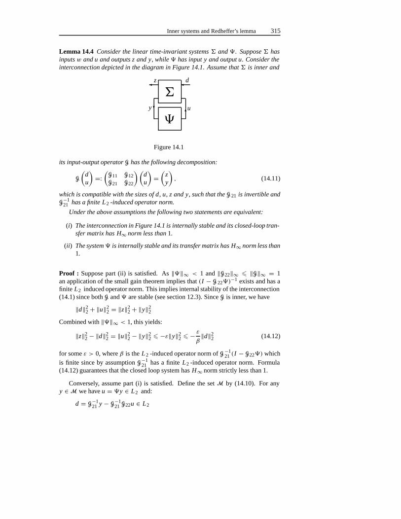
Inner systems and Redheffer’s lemma 315
Lemma 14.4 Consider the linear time-invariant systems � and � . Suppose � hasinputs w and u and outputs z and y, while � has input y and output u. Consider theinterconnection depicted in the diagram in Figure 14.1. Assume that � is inner and
�
��
�
�
�
y
z d
u
Figure 14.1
its input-output operator G has the following decomposition:
G
(du
)=:
(G11 G12G21 G22
)(du
)=
(zy
), (14.11)
which is compatible with the sizes of d, u, z and y, such that the G21 is invertible andG−1
21 has a finite L2 -induced operator norm.
Under the above assumptions the following two statements are equivalent:
(i) The interconnection in Figure 14.1 is internally stable and its closed-loop tran-sfer matrix has H∞ norm less than 1.
(ii) The system� is internally stable and its transfer matrix has H∞ norm less than1.
Proof : Suppose part (ii) is satisfied. As‖�‖∞ < 1 and‖G22‖∞ � ‖G‖∞ = 1an application of the small gain theorem implies that(I − G22�)
−1 exists and has afinite L2 induced operator norm. This implies internal stability of the interconnection(14.1) since bothG and� are stable (see section 12.3). SinceG is inner, we have
‖d‖22+ ‖u‖2
2 = ‖z‖22+ ‖y‖2
2
Combined with‖�‖∞ < 1, this yields:
‖z‖22− ‖d‖2
2 = ‖u‖22 − ‖y‖2
2 � −ε‖y‖22 � − ε
β‖d‖2
2 (14.12)
for someε > 0, whereβ is theL 2 -induced operator norm ofG−121 (I − G22�) which
is finite since by assumptionG−121 has a finiteL2 -induced operator norm. Formula
(14.12) guarantees that the closed loop system hasH∞ norm strictly less than 1.
Conversely, assume part (i) is satisfied. Define the setM by (14.10). For anyy ∈M we haveu = �y ∈ L2 and:
d = G−121 y − G−1
21 G22u ∈ L2
316 The H∞ control problem with measurement feedback
sinceG−121 has a finiteL2 -induced operator norm. But then:
‖u‖22− ‖y‖2
2 = ‖z‖22 − ‖d‖2 � −ε‖d‖2
2 � − εβ‖y‖2
2
for someε > 0, whereβ is theL 2 -induced operator norm of the closed loop systemmappingd to y which must be finite since the interconnected system is internallystable. Hence we get that
supy∈M,y =0
‖�y‖2
‖y‖2< 1. (14.13)
Then, by lemma 14.3, we know thatM is a closed subspace ofL 2 . SupposeM is notequal to the whole ofL 2 . Then there must be a signal 0= w ∈M⊥ ⊂ L2 . Since theclosed loop system is stable we know that�(I − G22�)
−1 and(I − G22�)−1 must
both be stable. But thenr = (I − G22�)−1w ∈ M. We get:
‖G22�r‖22 = ‖r −w‖2
2 = ‖r‖22 + ‖w‖2
2 � ‖r‖22 (14.14)
The second equality follows from the fact thatr ∈ M andw ∈ M⊥. But we knowthatr ∈ M guarantees that‖�r‖2 < ‖r‖ and we also know that‖G22‖∞ � 1 whichtogether contradict (14.14). HenceM = L 2 , which guarantees that� is stable, while(14.13) guarantees that‖�‖∞ < 1.
14.4 Proof of theorem 14.1
In this section theorem 14.1 will be proven. We will show that the problem of findinga suitable controller� for the system (14.1) is equivalent to finding a suitable con-troller � for a new system which has some very nice structural properties. We canshow that for this new system the disturbance decoupling problem with measurementfeedback and stability is solvable (see lemma 11.13). Clearly, this implies that we canfind for this new system, and hence also for our original system, a suitable controller.We recall that in the remainder of this chapter it is assumed thatγ = 1.
Lemma 14.5 Assume that the systems (A, B,C2, D2) and (A, E,C1, D1) have nozeros on the imaginary axis and assume that D1 and D2 are surjective and injective,respectively. If a controller � exists such that the resulting closed-loop system isinternally stable and has H∞ norm less than 1, then the following two conditions aresatisfied:
(i) There exists a real symmetric solution P � 0 of the algebraic Riccati equation(14.3) such that (14.5) is a stability matrix (with γ = 1).
(ii) There exists a symmetric solution Q � 0 of the algebraic Riccati equation(14.4) such that (14.6) is a stability matrix (with γ = 1).

Proof of theorem 14.1 317
Proof : Since there exists an internally stabilizing feedback controller that makes theH∞ norm of the closed-loop system less than 1 for the problem with measurementfeedback, it is easy to check that part (i) of theorem 13.3 is satisfied. Note that weneed to do some work because part (i) requires the existence of a static state feedbackand we have a dynamic function of both the state and the disturbance. But checkingthe proof of theorem 13.3, the existence of a matrixP satisfying the conditions inpart (i) of the above lemma is guaranteed when the expression (13.15) is boundedand if we make the suboptimal choice of determiningu on the basis of our dynamicmeasurement feedback it is not hard to see that (13.15) is indeed bounded.
For a system� = (F,G, H, J ), as before we define the dual system� T as thesystem with realization(F T, H T,GT, J T). It is not hard to see (using the frequencydomain interpretation of theH∞ norm) that theH∞ norm of a system is equal to theH∞ norm of its dual system. Define the dual system of�:
�T :xd = ATxd + CT
1ud + CT
2dd ,
yd = BTxd + DT
2dd ,
zd = ETxd + DT
1ud ,
and the dual of our controller�:
�TF : wd = K Twd + MT yd ,
ud = LTwd + N T yd .
It is easy to see that the dual system of� × � is equal to� T × �T. Therefore,since� stabilizes� and yields a closed loopH∞ norm less than 1, we have that�T
stabilizes�T and yields the same closed loopH∞ norm, less than 1. But then thestate feedbackH∞ control problem for� T is also solvable and by applying theorem13.3 (the required assumptions are satisfied since(A T,CT
1, ET, DT
1) has no zeros onthe imaginary axis andDT
1 is injective) we find that the Riccati equation related to� T
has a stabilizing real symmetric solution, sayQ, with Q � 0. This solution turns outto satisfy the conditions in part (ii) of our lemma.
Note that exercise 14.1 yields an alternative proof of part (ii) without resorting tothe concept of duality.
Assume that there exist matricesP and Q satisfying conditions (i) and (ii) inlemma 14.5. In the previous chapter we have seen that:
‖z‖22− ‖d‖2
2 = ‖D2(u − Fx)‖22− ‖d − E T Px‖2
2
whereF = −(DT
2D2)−1(BT P + DT
2C2). We definez P = D2(u − Fx) anddP =d− E T Px . Then from the above it is intuitively clear that if we find a controller fromy to u which makes theH∞ norm fromd to z less than 1 then the same controller willalso make theH∞ norm fromd P to z P equal to 1. This new system with disturbancedP , inputu, measurementy and to be controlled outputz P has the following form:
�P :x P = AP x P + Bu + EdP ,
y = C1,P x P + D1dP ,
z P = C2,P x P + D2u,(14.15)
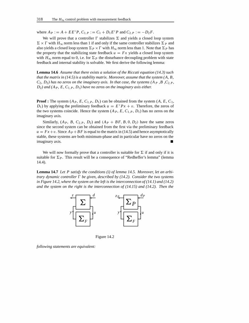
318 The H∞ control problem with measurement feedback
whereA P : = A + E E T P, C1,P : = C1+ D1ET P andC2,P : = −D2F .
We will prove that a controller� stabilizes� and yields a closed loop system� × � with H∞ norm less than 1 if and only if the same controller stabilizes� P andalso yields a closed loop system�P×� with H∞ norm less than 1. Note that�P hasthe property that the stabilizing state feedbacku = Fx yields a closed loop systemwith H∞ norm equal to 0, i.e. for�P the disturbance decoupling problem with statefeedback and internal stability is solvable. We first derive the following lemma:
Lemma 14.6 Assume that there exists a solution of the Riccati equation (14.3) suchthat the matrix in (14.5) is a stability matrix. Moreover, assume that the system (A, B,C2, D2) has no zeros on the imaginary axis. In that case, the systems (A P ,B ,C2,P ,D2) and (A P, E, C1,P , D1) have no zeros on the imaginary axis either.
Proof : The system (A P , E , C1,P , D1) can be obtained from the system (A, E , C1,D1) by applying the preliminary feedbacku = E T Px + v. Therefore, the zeros ofthe two systems coincide. Hence the system (A P , E , C1,P , D1) has no zeros on theimaginary axis.
Similarly, (A P , B, C2,P , D2) and (A P + B F, B,0, D2) have the same zerossince the second system can be obtained from the first via the preliminary feedbacku = Fx+v. SinceA P+B F is equal to the matrix in (14.5) and hence asymptoticallystable, these systems are both minimum-phase and in particular have no zeros on theimaginary axis.
We will now formally prove that a controller is suitable for� if and only if it issuitable for�P . This result will be a consequence of “Redheffer’s lemma” (lemma14.4).
Lemma 14.7 Let P satisfy the conditions (i) of lemma 14.5. Moreover, let an arbi-trary dynamic controller � be given, described by (14.2). Consider the two systemsin Figure 14.2, where the system on the left is the interconnection of (14.1) and (14.2)and the system on the right is the interconnection of (14.15) and (14.2). Then the
�
�F
�
�
�
�
y
z d
u
�P
�F
�
�
�
�
y
z P dP
u
Figure 14.2
following statements are equivalent:
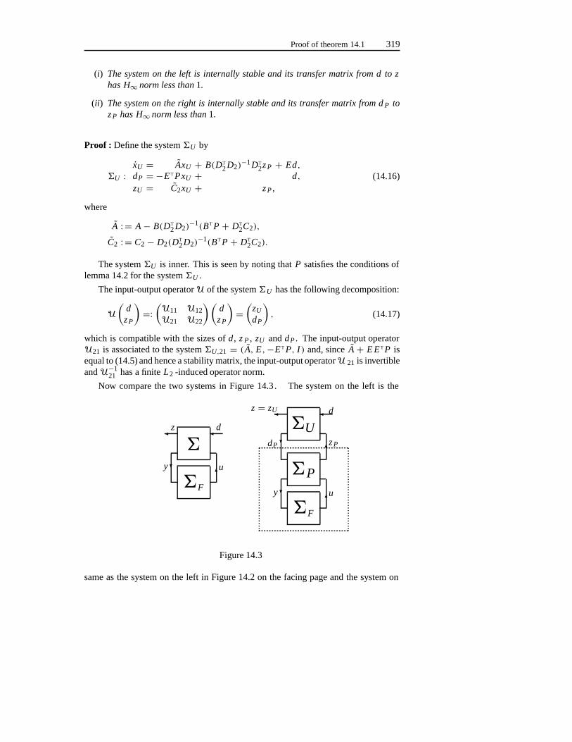
Proof of theorem 14.1 319
(i) The system on the left is internally stable and its transfer matrix from d to zhas H∞ norm less than 1.
(ii) The system on the right is internally stable and its transfer matrix from d P toz P has H∞ norm less than 1.
Proof : Define the system�U by
�U :xU = AxU + B(DT
2D2)−1DT
2z P + Ed,dP = −ET PxU + d,zU = C2xU + z P ,
(14.16)
where
A : = A − B(DT
2D2)−1(BT P + DT
2C2),
C2 : = C2 − D2(DT
2D2)−1(BT P + DT
2C2).
The system�U is inner. This is seen by noting thatP satisfies the conditions oflemma 14.2 for the system�U .
The input-output operatorU of the system�U has the following decomposition:
U
(d
z P
)=:
(U11 U12U21 U22
)(dz P
)=
(zU
dP
), (14.17)
which is compatible with the sizes ofd, z P , zU anddP . The input-output operatorU21 is associated to the system�U,21 = ( A, E,−E T P, I ) and, sinceA + E E T P isequal to (14.5) and hence a stability matrix, the input-output operatorU 21 is invertibleandU−1
21 has a finiteL2 -induced operator norm.
Now compare the two systems in Figure 14.3. The system on the left is the
�
�P�F
�F
�U
�
�
�
�
�
�
�
�
��
y
z d
u
z = zU
y u
d
dP z P
Figure 14.3
same as the system on the left in Figure 14.2 on the facing page and the system on
320 The H∞ control problem with measurement feedback
the right is described by the system (14.16) interconnected with the system on theright in Figure 14.2. The system on the right in Figure 14.3 on the preceding page isdescribed by:
xU − x P
x P
w
=
A + E E T P 0 0−(E + B N D1)ET P A + B NC1 B M
−L D1ET P LC1 K
xU − x P
x P
w
+ 0
E + B N D1L D1
d,
zU = (C2 − D2N D1ET P C2+ D2NC1 D2M
)xU − x P
x P
w
+D2N D1d.
If we also derive the system equations for the system on the left in Figure 14.3 on thepreceding page we get:(
x P
w
)=
(A + B NC1 B M
LC1 K
)(x P
w
)+
(E + B N D1
L D1
)d,
z = (C2+ D2NC1 D2M
) (x P
w
)+ D2N D1d.
We immediately see that, sinceA+E E T P is asymptotically stable, the two systems inFigure 14.3 on the preceding page have the same transfer matrix and one is internallystable if and only if the other one is internally stable. Hence the system on the left isstable and hasH∞ norm less than 1 if, and only if, the system on the right is stableand hasH∞ norm less than 1.
We can now apply lemma 14.4 to the system on the right in Figure 14.3 and hencewe find that the closed-loop system is internally stable and hasH∞ norm less than 1if, and only if, the dashed system is internally stable and hasH∞ norm less than 1.
Since the dashed system is exactly the system on the right in Figure 14.2 and thesystem on the left in Figure 14.3 is exactly equal to the system on the left in Figure14.2 we have completed the proof.
We assumed that for the original system (14.1) there exists an internally stabi-lizing controller such that the resulting closed-loop matrix hasH∞ norm less than1. Hence, by applying lemma 14.7, we know that thesame controller is internallystabilizing for the new system (14.15) and yields a closed-loop transfer matrix withH∞ norm less than 1. Moreover we know by lemma 14.6 that� satisfies the assump-tions on the invariant zeros needed to apply lemma 14.5. Therefore, if we considerfor this new system the two Riccati equations we know that there are positive semi-definite, stabilizing solutions. We shall now formalize this in the following lemma.
Proof of theorem 14.1 321
Consider the following Riccati equations:
ATP X + X AP + CT
2,PC2,P + X E E T X
− (X B + CT
2,P D2) (
DT
2D2)−1 (
BT X + DT
2C2,P) = 0, (14.18)
APY + Y AT
P + E ET + Y CT
2,PC2,PY
− (Y CT
1,P + E DT
1
) (D1DT
1
)−1 (C1,PY + D1ET
) = 0, (14.19)
in the unknownsX andY in Rn×n . In addition, for givenX,Y consider the followingtwo matrices:
AP + E ET X − B(DT
2D2)−1(BT X + DT
2C2,P), (14.20)
AP + Y CT
2,PC2,P −(Y CT
1,P + E DT
1
) (D1DT
1
)−1C1,P . (14.21)
Then we have:
Lemma 14.8 Let P and Q satisfy conditions (i) and (ii) in lemma 14.5. Then wehave the following two results:
(i) X = 0 is a solution of the algebraic Riccati equation (14.18) such that (14.20)is stable.
(ii) The algebraic Riccati equation (14.19) has a real symmetric matrix Y such that(14.21) is a stability matrix if and only if I−Q P is invertible. Moreover, in thiscase there is a unique solution Y : = (I − Q P)−1 Q. This matrix Y is positivesemi-definite if and only if
ρ (P Q) < 1. (14.22)
Proof : Part (i) can be checked straightforwardly.
We know thatQ is the stabilizing solution of the algebraic Riccati equation (14.4).Using the results from section 13.4 we know therefore
Xold = im
(IQ
)
is theC−-stable subspace of the Hamiltonian matrix:
Hold =(
AT − CT
1(D1DT
1)−1D1ET CT
2C2 − CT
1(D1DT
1)−1C1
−E[I − DT
1(D1DT
1)−1D1
]ET −A + E DT
1(D1DT
1)−1C1
).
Define a new Hamiltonian matrix by
Hnew =(
I −P0 I
)Hold
(I P0 I
). (14.23)
322 The H∞ control problem with measurement feedback
It is then easy to check that forY to be a stabilizing solution of the algebraic Riccatiequation (14.19) requires that
Xnew = im
(IY
)
is theC−-stable subspace of the Hamiltonian matrixHnew. However, (14.23) impliesthat theC−-stable subspace ofHnew is equal to:
im
(I −P0 I
)(IQ
)= im
(I − P Q
Q
).
Therefore we know that a stabilizing solution to the algebraic Riccati equation (14.21)exists if and only ifI − P Q is invertible and in this case the solution is given byY = Q (I − P Q)−1. The requirementY � 0 is satisfied if and only ifρ(P Q) < 1,which can be checked by noting that:
Y = Q1/2(
I − Q1/2P Q1/2)−1
Q1/2
andρ(P Q) = ρ(Q1/2P Q1/2). This completes the proof.
This completes the proof of the implication (i)⇒ (ii) in theorem 14.1. Theexistence ofP � 0 and Q � 0 satisfying the algebraic Riccati equations (14.3)and (14.4) such that the matrices (14.5) and (14.6) are stability matrices can be ob-tained directly from lemma 14.5. We know by lemma 14.6 that the two subsystems(AP , B,C2,P , D2) and(A P , E,C1,P , D1) have no zeros on the imaginary axis. Wealso know by lemma 14.7 that a controller exists for the transformed system� P
which internally stabilizes the system and makes theH∞ norm of the closed-loopsystem less than 1. By applying lemma 14.5 to this new system we find that a matrixY � 0 exists that satisfies the algebraic Riccati equation (14.19), such that (14.21)is a stability matrix. Hence by lemma 14.8 we have (14.22) and therefore all theconditions in theorem 14.1, part (ii) are satisfied.
We will now prove the reverse implication (ii)⇒ (i) in theorem 14.1. Hence,assume that matricesP andQ exist satisfying the conditions of part (ii) of theorem14.1.
In order to prove the implication (ii)⇒ (i) we transform the system (14.15) onceagain, this time however using the dualized version of the original transformation. Inother words, we define the dual system� T
P , apply the same transformation from�to �P , but this time we transform� T
P into a new system which we call�TP Q and
when we dualize�T
P Q we obtain our new system�P Q . The transformation from� to�P depended on the solution of a Riccati equation which is determined by therealization of�. This time we have to solve a similar Riccati equation for� T
P Itturns out this Riccati equation is equal to (14.19) and has, by lemma 14.8, a solutionY = (I − Q P)−1 Q � 0.
Proof of theorem 14.1 323
In the way described above, we obtain the following system:
�P Q :x P Q = AP Q x P Q + BP Qu + E P QdP Q,
y = C1,P x P Q + D1dP Q,
z P Q = C2,P x P Q + D2u,(14.24)
where
AP Q : = AP + Y CT
2,PC2,P ,
BP Q : = B + Y CT
2,P D2,
E P Q : = (Y CT
1,P + E DT
1)(D1DT
1)−1D1.
By applying lemma 14.7 and its dualized version, the following corollary can bederived:
Corollary 14.9 Let � be a controller of the form (14.2). The following two state-ments are equivalent:
(i) The controller � applied to the system � described by (14.1) is internally sta-bilizing, and the resulting closed-loop transfer matrix has H∞ norm less than1.
(ii) The controller � applied to the system �P Q described by (14.24) is internallystabilizing, and the resulting closed-loop transfer matrix has H∞ norm lessthan 1.
Remark : We note that, even if for this new system we can make theH∞ normarbitrarily small, for the original system we are only sure that theH∞ norm will beless than 1. It is possible that a controller for the new system yields anH∞ norm ofsay 0.0001 while the same controller makes theH∞ norm of the original plant only0.9999.
We can apply the following controller to� P Q :
� : ˙x P Q = AP Q x P Q + BP Qu + K (y − C1,P x P Q),
u = Fx P Q ,(14.25)
where
K = (Y CT
1,P + E DT
1)(D1DT
1)−1,
F = −(DT
2D2)−1(DT
2C2 + BT P).
Note that
AP Q + BP Q F = (AP + B F)+ Y CT
2,P(C2,P + D2F) = A + E E T P + B F,
AP Q − K C1,P = AP + Y CT
2,PC2,P − K C1,P ,
324 The H∞ control problem with measurement feedback
which are equal to the matrices in (14.5) and (14.21) respectively and hence stabilitymatrices. It is then easy to check that the resulting closed loop system� P Q × � isstable and achieves disturbance decoupling with measurement feedback and internalstability (see section 11.3). Hence by applying corollary 14.9 we see that this con-troller satisfies part (i) of theorem 14.1. This completes the implication (ii)⇒ (i)in theorem 14.1. Note that the controller (14.25) is equal to the controller given intheorem 14.1.
14.5 Characterization of all suitable controllers
In this section we will parameterize all stabilizing controllers which achieve the re-quiredH∞ norm bound. We assume throughout this section that there exist matricesP andQ satisfying the conditions of part (ii) of theorem 14.1.
Let � and�P Q be defined by (14.1) and (14.24) respectively. We define thefollowing system:
�P Q :x P Q = AP Q x P Q + BP Qu + E P QdP Q ,
y = C1,P x P Q + (D1DT
1)1/2dP Q ,
z P Q = C2,P x P Q + (DT
2D2)1/2u,
(14.26)
where
C2,P : = (DT
2D2)−1/2(BT P + DT
2C2),
E P Q : = (Y CT
1,P + E DT
1)(D1DT
1)−1/2.
We have�P Q = 2�P Q1 where
1 = (D1DT
1)−1/2D1 and2 = D2(D
T
2D2)−1/2.
Hence, it is straightforward that the class of stabilizing controllers for� P Q is equalto the class of stabilizing controllers for�P Q . Moreover, for any interconnection�P Q × � where� stabilizes�, we get a closed loop transfer matrixQ = 2X1whereX is the stable closed loop transfer matrix of�P Q×�. The system�P Q turnsout to have a very special property:
Lemma 14.10 Let �P Q be given. For any internally stable system �x with transfermatrix X there exists a controller which stabilizes �P Q and which yields a closedloop transfer matrix equal to X.
Proof : Consider the following system.
�e :xc = AP Q xc + BP Qu + K (y − C1,P xc),
dx = (D1DT
1)−1/2[y − C1,P xc],
u = (DT
2D2)−1/2[zx − C2,P xc].
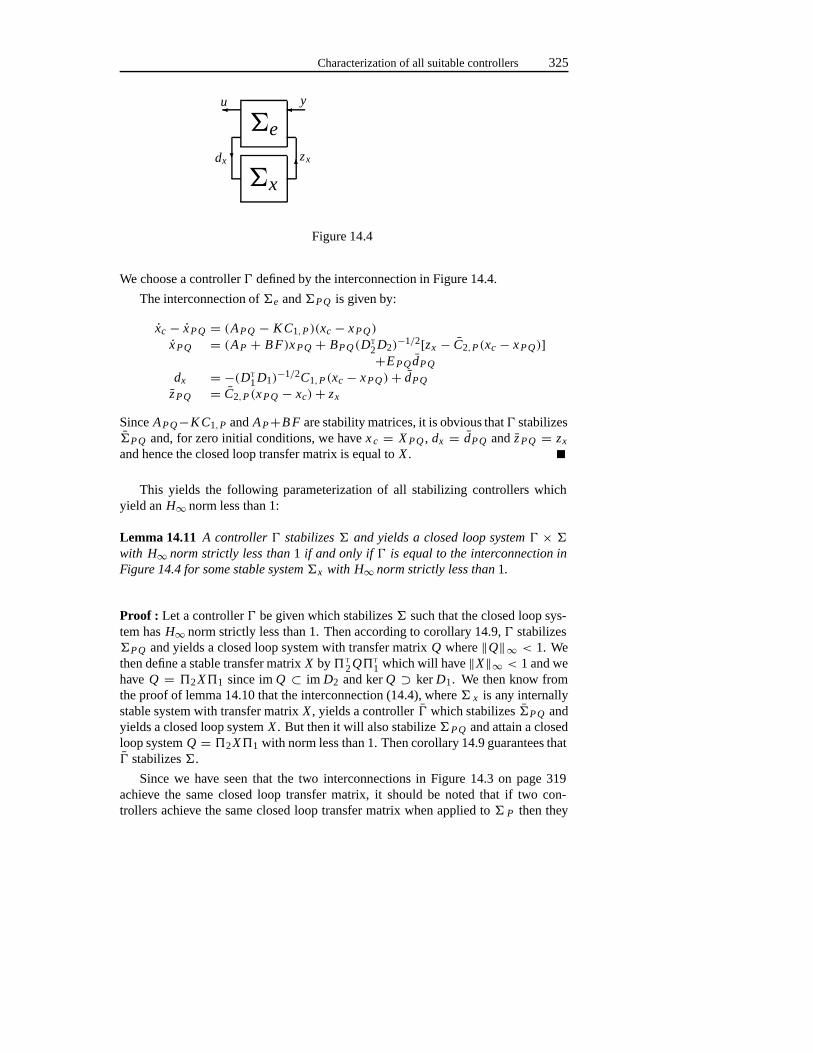
Characterization of all suitable controllers 325
�e
�x
�
�
�
�
dx
u y
zx
Figure 14.4
We choose a controller� defined by the interconnection in Figure 14.4.
The interconnection of�e and�P Q is given by:
xc − x P Q = (AP Q − K C1,P)(xc − x P Q)
x P Q = (AP + B F)x P Q + BP Q(DT
2D2)−1/2[zx − C2,P(xc − x P Q)]
+E P QdP Q
dx = −(DT
1D1)−1/2C1,P (xc − x P Q)+ dP Q
z P Q = C2,P (x P Q − xc)+ zx
SinceAP Q−K C1,P andA P+B F are stability matrices, it is obvious that� stabilizes�P Q and, for zero initial conditions, we havex c = X P Q , dx = dP Q andz P Q = zx
and hence the closed loop transfer matrix is equal toX .
This yields the following parameterization of all stabilizing controllers whichyield anH∞ norm less than 1:
Lemma 14.11 A controller � stabilizes � and yields a closed loop system � × �with H∞ norm strictly less than 1 if and only if � is equal to the interconnection inFigure 14.4 for some stable system �x with H∞ norm strictly less than 1.
Proof : Let a controller� be given which stabilizes� such that the closed loop sys-tem hasH∞ norm strictly less than 1. Then according to corollary 14.9,� stabilizes�P Q and yields a closed loop system with transfer matrixQ where‖Q‖∞ < 1. Wethen define a stable transfer matrixX byT
2QT
1 which will have‖X‖∞ < 1 and wehaveQ = 2X1 since imQ ⊂ im D2 and kerQ ⊃ kerD1. We then know fromthe proof of lemma 14.10 that the interconnection (14.4), where� x is any internallystable system with transfer matrixX , yields a controller� which stabilizes�P Q andyields a closed loop systemX . But then it will also stabilize�P Q and attain a closedloop systemQ = 2X1 with norm less than 1. Then corollary 14.9 guarantees that� stabilizes�.
Since we have seen that the two interconnections in Figure 14.3 on page 319achieve the same closed loop transfer matrix, it should be noted that if two con-trollers achieve the same closed loop transfer matrix when applied to� P then they
326 The H∞ control problem with measurement feedback
also achieve the same closed loop transfer matrix when applied to�. Since the con-nection between�P and�P Q is dual to the connection between� and� P , weobtain that two controllers achieve the same closed loop transfer matrix when appliedto�P Q then they also achieve the same closed loop transfer matrix when applied to�P . In conclusion, since we know that� and � yield the same closed loop transfermatrix when applied to�P Q , we have that� yields the same closed loop transfermatrix as� when applied to�. Partition the transfer matrixG of � into�:
G =(
G11 G12G21 G22
)(14.27)
compatible with the partitioning of(d, u) and)(z, y). Let C and C be the transfermatrices associated to� and� respectively. We have:
G11+ G12C(I − G22C)−1G21 = G11+ G12C(I − G22C)−1G21.
SinceG21(∞) is surjective andG12(∞) is injective we get that the associated transfermatrices are surjective and injective respectively. Hence:
C(I − G22C)−1 = C(I − G22C)−1,
which yields
(I − CG22)C = C(I − G22C).
HenceC = C , which proves that� and � are the same or, in other words, our con-troller � is equal to the interconnection (14.4) for a stable system� x with H∞ normstrictly less than 1.
Conversely, suppose a stable�x is given whose transfer matrixX hasH∞ normless than 1. Define by� the controller given by the interconnection (14.4). Thenlemma 14.10 guarantees that� stabilizes�P Q and hence also stabilizes�P Q . More-over the closed loop transfer matrix of the interconnection of� P Q and� is equal to2X1 and hasH∞ norm strictly less then 1. Corollary 14.9 then guarantees that�
stabilizes� and yields a closed loop system withH∞ norm strictly less than 1.
Note that the above theorem parameterizes the class of all suitable controllers�
by all stable systems withH∞ norm strictly less than 1. The controller we obtain for�x equal to 0 is in a certain sense the center of the parameterization and is henceoften called thecentral controller. The controller given in theorem 14.1, turns out tobe equal to this central controller.
14.6 Exercises
14.1 The dualization argument used in the proof of lemma 14.5 is of course validbut it is sometimes hard to get a good feeling for it. There is another derivation
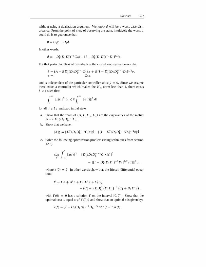
Exercises 327
without using a dualization argument. We knowd will be a worst-case dist-urbance. From the point of view of observing the state, intuitively the worstdcould do is to guarantee that:
0= C1x + D1d.
In other words:
d = −DT
1(D1DT
1)−1C1x + [I − DT
1(D1DT
1)−1D1]1/2v.
For that particular class of disturbances the closed loop system looks like:
x = (A − E DT
1(D1DT
1)−1C1
)x + E[I − DT
1(D1DT
1)−1D1]1/2v,
z = C2x ,
and is independent of the particular controller sincey = 0. Since we assumethere exists a controller which makes theH∞ norm less than 1, there existsδ < 1 such that:∫ ∞
0‖z(t)‖2 dt � δ
∫ ∞
0‖d(t)‖2 dt
for all d ∈ L2 and zero initial state.
a. Show that the zeros of(A, E,C1, D1) are the eigenvalues of the matrixA − E DT
1(D1DT
1)−1C1.
b. Show that we have:
‖d‖22 = ‖DT
1(D1DT
1)−1C1x‖2
2+ ‖[I − DT
1(D1DT
1)−1D1]1/2v‖2
2
c. Solve the following optimization problem (using techniques from section12.6)
supv
∫ 0
−T‖z(t)‖2 − ‖DT
1(D1DT
1)−1C1x(t)‖2
− ‖[I − DT
1(D1DT
1)−1D1]1/2v(t)‖2 dt .
wherex(0) = ξ . In other words show that the Riccati differential equa-tion:
Y = Y A + ATY + Y E ETY + CT
2C2
− (CT
1+ Y E DT
1
) (D1DT
1
)−1 (C1 + D1ETY
),
with Y (0) = 0 has a solutionY on the interval[0, T ]. Show that theoptimal cost is equal toξ TY (T )ξ and show that an optimalv is given by:
v(t) = [I − DT
1(D1DT
1)−1D1]1/2ETY (t + T )x(t).
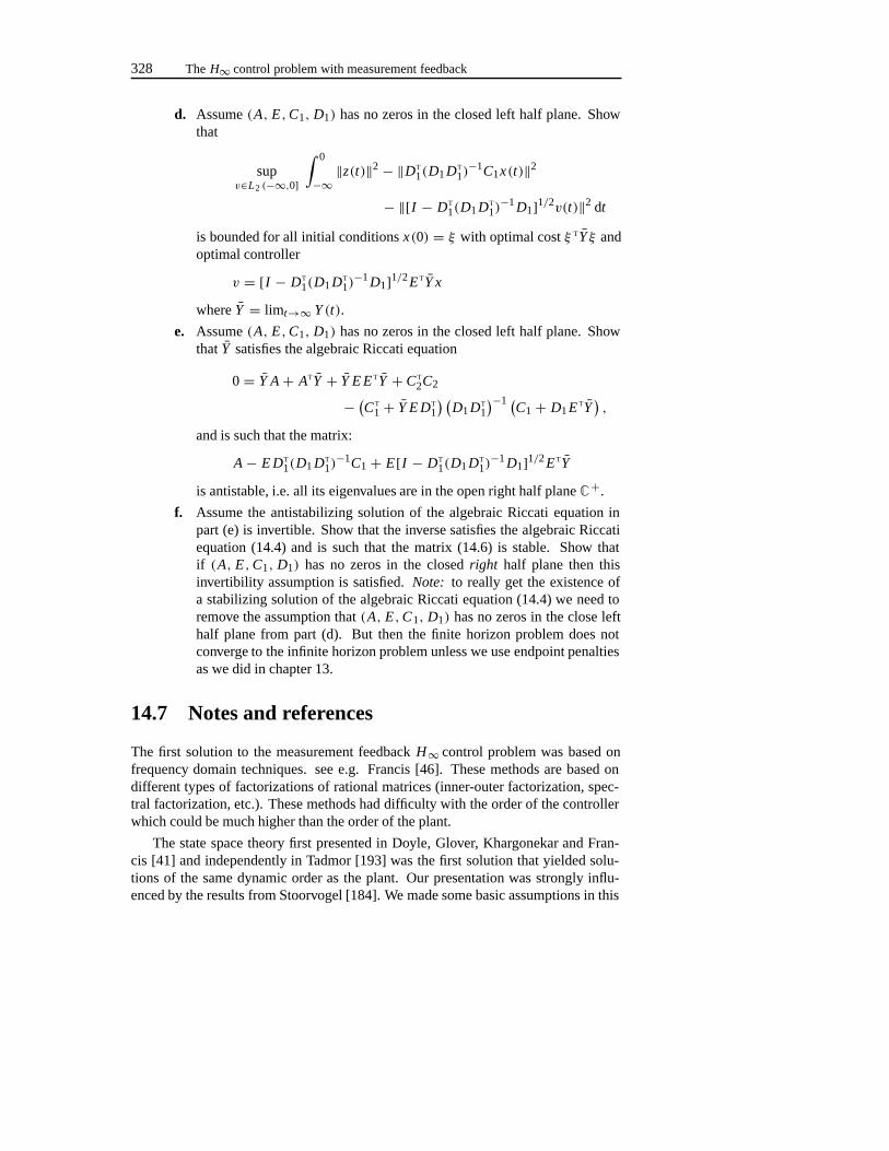
328 The H∞ control problem with measurement feedback
d. Assume(A, E,C1, D1) has no zeros in the closed left half plane. Showthat
supv∈L2 (−∞,0]
∫ 0
−∞‖z(t)‖2 − ‖DT
1(D1DT
1)−1C1x(t)‖2
− ‖[I − DT
1(D1DT
1)−1D1]1/2v(t)‖2 dt
is bounded for all initial conditionsx(0) = ξ with optimal costξ TY ξ andoptimal controller
v = [I − DT
1(D1DT
1)−1D1]1/2ETY x
whereY = limt→∞ Y (t).
e. Assume(A, E,C1, D1) has no zeros in the closed left half plane. ShowthatY satisfies the algebraic Riccati equation
0= Y A + ATY + Y E ETY + CT
2C2
− (CT
1+ Y E DT
1
) (D1DT
1
)−1 (C1 + D1ETY
),
and is such that the matrix:
A − E DT
1(D1DT
1)−1C1+ E[I − DT
1(D1DT
1)−1D1]1/2ETY
is antistable, i.e. all its eigenvalues are in the open right half planeC+.
f. Assume the antistabilizing solution of the algebraic Riccati equation inpart (e) is invertible. Show that the inverse satisfies the algebraic Riccatiequation (14.4) and is such that the matrix (14.6) is stable. Show thatif (A, E,C1, D1) has no zeros in the closedright half plane then thisinvertibility assumption is satisfied.Note: to really get the existence ofa stabilizing solution of the algebraic Riccati equation (14.4) we need toremove the assumption that(A, E,C1, D1) has no zeros in the close lefthalf plane from part (d). But then the finite horizon problem does notconverge to the infinite horizon problem unless we use endpoint penaltiesas we did in chapter 13.
14.7 Notes and references
The first solution to the measurement feedbackH∞ control problem was based onfrequency domain techniques. see e.g. Francis [46]. These methods are based ondifferent types of factorizations of rational matrices (inner-outer factorization, spec-tral factorization, etc.). These methods had difficulty with the order of the controllerwhich could be much higher than the order of the plant.
The state space theory first presented in Doyle, Glover, Khargonekar and Fran-cis [41] and independently in Tadmor [193] was the first solution that yielded solu-tions of the same dynamic order as the plant. Our presentation was strongly influ-enced by the results from Stoorvogel [184]. We made some basic assumptions in this
Notes and references 329
chapter: no invariant zeros on the imaginary axis and direct feedthough matrices thatshould have full rank. The case when these assumptions are not satisfied is referredto as the singular case and will be discussed in the next chapter. The addition of di-rect feedthrough matrices fromu to y or fromw to z, can be approached using thetechniques presented in Safonov, Limebeer and Chiang [160]. The general results inthis case (regular but all direct feedthrough matrices present) can be found in Gloverand Doyle [62].
In the last few years this frequency domain approach has been refined via the in-troduction of the so-calledJ -spectral factorization (see e.g. Green, Glover, Limebeerand Doyle [65]). At the moment this is quite an elegant theory and does not suffer anylonger from the drawbacks of high-order controllers that were present in the originalfrequency domain methods. Another recent development is to solve theH∞ controlproblem via linear matrix inequalities (LMI). See, for instance, Gahinet [53] andIwasaki and Skelton [88]. Other techniques to solveH∞ are based on interpolationmethods, Limebeer and Anderson [110] and Zames and Francis [231] and polynomialmethods, see Kwakernaak [103,104].
In this chapter we prove the existence of solutions of the second Riccati equationand the existence of a suitable observer via duality. A beautiful interpretation of thissecond (observer) Riccati equation is presented in Khargonekar [100] by connectingit to the behavior of the zero dynamics, i.e. the behavior of the system under theconstrainty = 0.
The theory ofH∞ has been extended to infinite dimensional systems. See, forinstance, van Keulen [205] and the special issue [34]. Extensions to time-varyingsystems also exist. See for instance Limebeer, Anderson, Khargonekar, and Green[111] and Ravi, Nagpal and Khargonekar [152].
The discrete-time version ofH∞ has also been studied in detail. See for instanceIglesias and Glover [84], Stoorvogel [184] and Stoorvogel, Saberi and Chen [188].

330 The H∞ control problem with measurement feedback
Chapter 15
Some applications of theH∞ control problem
15.1 Introduction
In chapter 12, we formulated a number of problems related to robust stabilizationwith additive, multiplicative or coprime factor model uncertainty. In this chapter,we would like to revisit these problems and see how the theory of the previous twochapter can give us additional insight.
We also like to consider in some detail what to do if some of the basic assump-tions in H∞ are not satisfied. These so-called singular problems are quite difficultbut by presenting some ad-hoc techniques we hope to provide the reader with someadditional insight for the difficulty of these problems.
Minimum entropy is an interpretation of the so-called central controller. It isuseful to study this interpretation because it yields additional insight in the relationbetweenH∞ andH2 .
Finally, for those people who are familiar with classical control, we present adesign example that might help to clarify the relations between classical control andH∞ .
15.2 Robustness problems and theH∞ control problem
In section 12.4 we discussed stabilization of uncertain systems. In the present sectionwe will apply the results of the previous two chapters to the three different types ofuncertainty described in that section:
• Additive perturbations
• Multiplicative perturbations
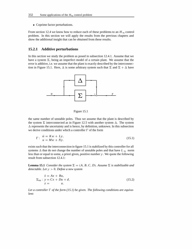
332 Some applications of theH∞ control problem
• Coprime factor perturbations.
From section 12.4 we know how to reduce each of these problems to anH∞ controlproblem. In this section we will apply the results from the previous chapters andshow the additional insight that can be obtained from these results.
15.2.1 Additive perturbations
In this section we study the problem as posed in subsection 12.4.1. Assume that wehave a system�, being an imperfect model of a certain plant. We assume that theerror is additive, i.e. we assume that the plant is exactly described by the interconnec-tion in Figure 15.1. Here,� is some arbitrary system such that� and� + � have
�
�
� � � �
�
� �
�
u y◦+
Figure 15.1
the same number of unstable poles. Thus we assume that the plant is described bythe system� interconnected as in Figure 12.5 with another system�. The system� represents the uncertainty and is hence, by definition, unknown. In this subsectionwe derive conditions under which a controller� of the form
� : w = Kw + Ly,u = Mw + Ny.
(15.1)
exists such that the interconnection in figure 15.1 is stabilized by this controller for allsystems� that do not change the number of unstable poles and that haveL ∞ normless than or equal to some, a priori given, positive numberγ . We quote the followingresult from subsection 12.4.1:
Lemma 15.1 Consider the system � = (A, B,C, D). Assume � is stabilizable anddetectable. Let γ > 0. Define a new system
�na :x = Ax + Bu,y = Cx + Du + d,z = u.
(15.2)
Let a controller � of the form (15.1) be given. The following conditions are equiva-lent:
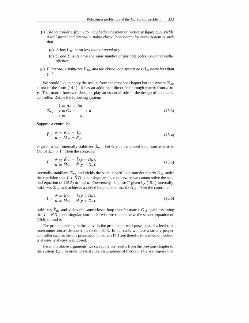
Robustness problems and theH∞ control problem 333
(i) The controller � from y to u applied to the interconnection in figure 12.5, yieldsa well-posed and internally stable closed loop system for every system � suchthat
(a) � has L∞ norm less than or equal to γ .
(b) � and � + � have the same number of unstable poles, counting multi-plicities.
(ii) � internally stabilizes �na , and the closed loop system has H∞ norm less thanγ−1.
We would like to apply the results from the previous chapter but the system� na
is not of the form (14.1). It has an additional direct feedthrough matrix fromd toy. That matrix however, does not play an essential role in the design of a suitablecontroller. Define the following system:
�na :x = Ax + Bu,y = Cx + d,z = u.
(15.3)
Suppose a controller
� : w = Kw + L y,u = Mw + N y,
(15.4)
is given which internally stabilizes�na . Let Gcl be the closed loop transfer matrixGcl of �na × �. Then the controller
� : w = Kw + L(y − Du),u = Mw + N(y − Du).
(15.5)
internally stabilizes�na and yields the same closed loop transfer matrixG cl underthe condition thatI + N D is nonsingular since otherwise we cannot solve the sec-ond equation of (15.5) to findu. Conversely, suppose� given by (15.1) internallystabilizes�na , and achieves a closed loop transfer matrixG cl . Then the controller
� : w = Kw + L(y + Du),u = Mw + N(y + Du).
(15.6)
stabilizes�na and yields the same closed loop transfer matrixG cl again assumingthat I − N D is nonsingular, since otherwise we can not solve the second equation of(15.6) to findu.
The problem arising in the above is the problem of well-posedness of a feedbackinterconnection as discussed in section 3.13. In our case, we have a strictly propercontroller such as the one presented in theorem 14.1 and therefore the interconnectionis always is always well posed.
Given the above arguments, we can apply the results from the previous chapter tothe system�na . In order to satisfy the assumptions of theorem 14.1 we impose that
334 Some applications of theH∞ control problem
A no eigenvalues on the imaginary axis. Then theorem 14.1 states that an internallystabilizing controller for the system�na exists which yields anH∞ norm less thanγif and only if there exist positive semi-definite real symmetric solutions of the Riccatiequations
AT P + P A − P B B T P = 0, (15.7)
AQ + Q AT − QCTC Q = 0, (15.8)
such thatρ(P Q) < γ 2 and such that the matricesA − B B T P and A + QC TC arestability matrices. Note thatP and Q do not depend onγ . Moreover, the resultsfrom chapter 10 guarantee the existence real symmetric solutionsP andQ of (15.7)and (15.8) such thatA − B B T P and A + QC TC are stability matrices. We see thata stabilizing controller for�na exists with a closed loop norm strictly less thanγ ifand only ifγ is larger thanρ(P Q)1/2.
We thus find the following theorem:
Theorem 15.2 Assume that � = (A, B,C, D) is stabilizable and detectable. As-sume that A has no eigenvalues on the imaginary axis. We define the related system�na by (15.2) and let γ > 0. The following conditions are equivalent:
(i) There exists a controller � from y to u of the form (15.1) such that, whenapplied to the interconnection (15.1), the closed-loop system is well posed andinternally stable for all systems � for which
(a) � has L∞ norm less than or equal to γ ,
(b) � and � +� have the same number of unstable poles.
(ii) We have ρ(P Q) < γ −2, where P and Q are the solutions of the algebraicRiccati equations (15.7) and (15.8) for which A − B B T P and A + QC TC arestability matrices..
Moreover, if P and Q satisfy part (ii), a controller satisfying part (i) is described by:
˙x = Ax + Bu + L(y − Cx − Du),u = −BT Px,
where L : = (I − γ 2Q P)−1QCT.
Remarks:
• Naturally the class of perturbations we have chosen is rather artificial. How-ever, it is easy to show that, if we allow for perturbations which additionalunstable poles, then there are arbitrarily small perturbations which destabilizethe closed-loop system. On the other hand, our class of perturbations doesinclude all stable systems� with H∞ norm less than or equal toγ .
Robustness problems and theH∞ control problem 335
• We want to find a controller satisfying part (i) for aγ which is as large aspossible. Note that part (ii) shows that, in fact, for everyγ smaller than thebound[ρ(P Q)]−1/2 we can find a controller satisfying part (i). Actually thereexists a controller which makes theH∞ norm equal to[ρ(P Q)]−1/2 which isclearly the best we can do.
• It can be shown that the bound[ρ(P Q)]−1/2 depends only on the unstabledynamics of�. Hence we could assume a priori thatA has only eigenvalues inthe open right half complex plane (we still have to exclude eigenvalues on theimaginary axis). In that case it can be shown thatP andQ are the inverses ofX andY , respectively, whereX andY are the unique positive definite solutionsof the following two Liapunov equations:
AX + X AT = B BT,
ATY + Y A = CTC.
Recall thatX and Y are referred to as the controllability and observabilitygramian respectively (see section 3.8).
15.2.2 Multiplicative perturbations
In this subsection we study the problem as posed in subsection 12.4.2.
We assume that, once again, we have a system� being an imperfect model of acertain plant. This time, we study multiplicative uncertainty, i.e. we assume that theplant is exactly described by the interconnection in Figure 15.2.
�
�
� � � �
�
� �
�
u y◦+
Figure 15.2
Here,� is some arbitrary system describing the uncertainty such that the intercon-nection in figure 15.2 has the same number of unstable poles (counting multiplicities)as�. In subsection 12.4.2, we have derived the following result
Lemma 15.3 Assume that � = (A, B,C, D) is stabilizable and detectable. Definea new system:
�nm :x = Ax + Bu + Bd,y = Cx + Du + Dd,z = u.
(15.9)
336 Some applications of theH∞ control problem
Let a controller � of the form (15.1) be given. The following conditions areequivalent:
(i) The controller � from y to u applied to the interconnection in figure 15.2, yieldsa well-posed and internally stable closed loop system for every system � suchthat
(a) � has L∞ norm less than or equal to γ ,
(b) The interconnection (15.2) has the same number of unstable poles as �.
(ii) � internally stabilizes �nm and the closed loop system has H∞ norm less thanγ−1.
Thus, we find that our original problem formulation is equivalent to the problemof finding an internally stabilizing controller for�nm which makes theH∞ normof the closed-loop system less thanγ −1. We would like to apply the results of theprevious chapter to this problem. Note that, as in the previous subsection, we have adirect feedthrough matrix fromu to y. The latter was not treated in chapter 14 but wehave seen in the previous subsection that we can design a controller for the auxiliarysystem:
�nm :x = Ax + Bu + Bd,y = Cx + Dd,z = u,
(15.10)
and via a simple transformation, find a controller for the original system� nm . Inorder to satisfy the assumptions of theorem 14.1 we require that(A, B,C, D) has nozeros on the imaginary axis, thatA has no poles on the imaginary axis and thatD issurjective.
The results of chapter 10 tell us that algebraic Riccati equations
AT Pm + Pm A − Pm B BT Pm = 0, (15.11)
and
AQm + Qm AT + B BT − (QmCT + B DT)(DDT)−1(C Qm + DBT) = 0, (15.12)
have a real symmetric solutionPm andQm for which the matricesA − B B T Pm andA − (QmCT + B DT)(DDT)−1C are stability matrices. By applying theorem 14.1 tothe system�nm , we find the following theorem:
Theorem 15.4 Let � = (A, B,C, D) be stabilizable and detectable. Let γ > 0.Assume that A has no eigenvalues on the imaginary axis, D is surjective, and (A, B,C, D) has no zeros on the imaginary axis. Under these assumptions the followingconditions are equivalent:
(i) A controller � from y to u of the form (15.1) exists which, when applied tothe interconnection (15.2), yields a closed-loop system that is well posed andinternally stable for all systems � such that:
Robustness problems and theH∞ control problem 337
(a) � has L∞ norm less than or equal to γ .
(b) The interconnection (15.2) and � have the same number of unstablepoles.
(ii) Either A is a stability matrix or 1+ ρ(Pm Qm) < γ−2.
If part (ii) is satisfied then a controller satisfying the conditions of part (i) is given byu = 0 if A is stable, and otherwise by:
˙x = (A − B BT Pm)x + L(y − Cx + DBT Pm x)u = (γ 2− 1)−1BT Pm x
where
L : =(
I − γ 2Qm Pm
1− γ 2
)−1
(B DT + QmCT)(DDT)−1.
Proof : We apply theorem 14.1 to the system�nm and we have to investigate fourcases:
• A is stable: the matricesP : = 0 andQ : = Qm satisfy condition (ii) of theorem14.1.
• A is not stable and γ < 1: we define
P : = Pm
1− γ 2, Q : = Qm (15.13)
Then it is straightforward to check thatP and Q are the unique matrices sat-isfying all requirements of condition (ii) of theorem 14.1 for� nm except forpossibly the condition on the spectral radius ofP Q. Moreover,Pm and Qm
satisfy 1+ ρ(Pm Qm) < γ−2 if, and only if, P andQ satisfy the requirementρ(P Q) < γ−2 (note that we have to replaceγ by γ −1).
• A is not stable and γ = 1: the stability requirement forP reduces to therequirement thatA is stable which, by assumption, is not true.
• A is not stable and γ > 1: the matricesP and Q given by (15.13) are thestabilizing solutions of the two Riccati equations of part (iii) of theorem 14.1.We have seen in section 13.4 that the stabilizing solution is unique. However,the matrixP is not positive semi-definite. Therefore the conditions of part (ii)of theorem 14.1 are not satisfied.
Therefore theorem 14.1 guarantees that a suitable controller exists for�nm if andonly if the conditions of part (ii) of theorem 15.4 are satisfied. But the existence of asuitable controller for�nm is equivalent to the existence of a suitable controller for�nm as argued in the previous subsection.
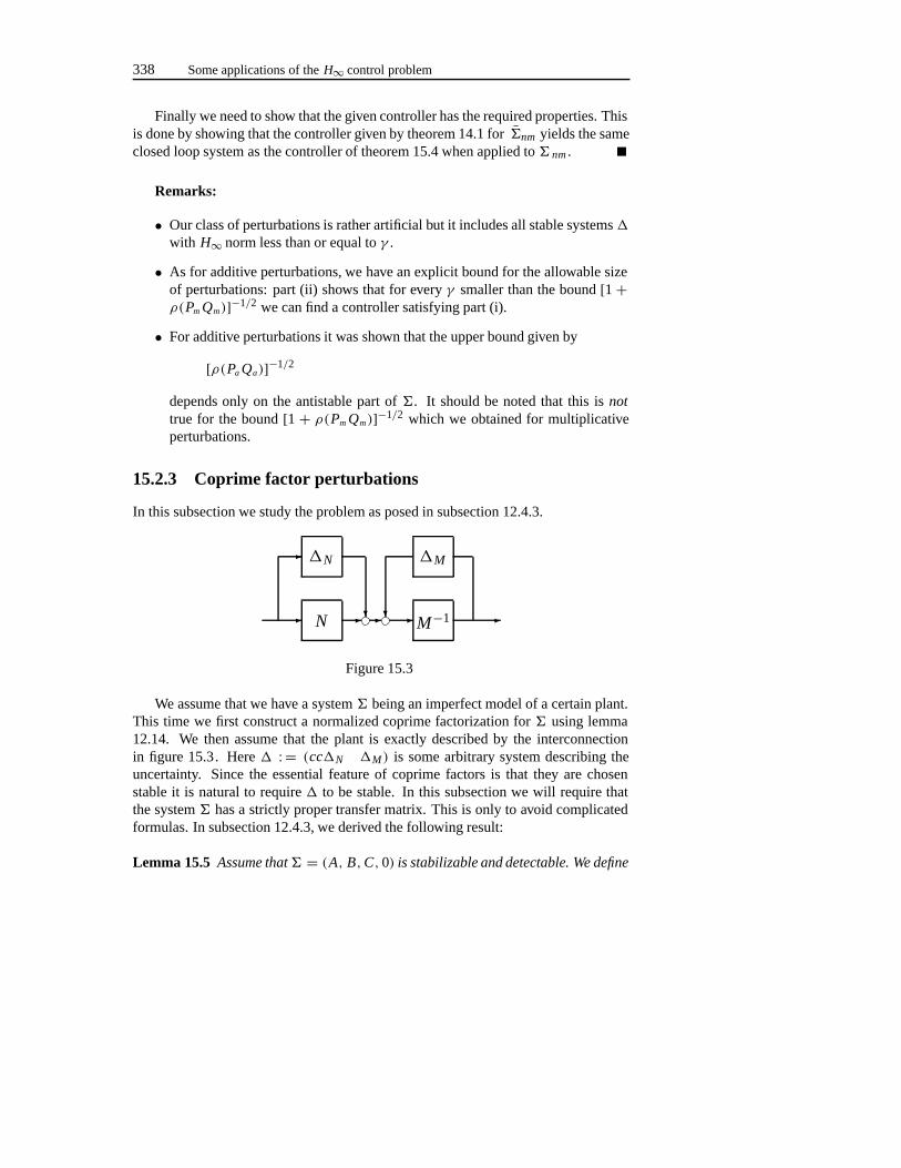
338 Some applications of theH∞ control problem
Finally we need to show that the given controller has the required properties. Thisis done by showing that the controller given by theorem 14.1 for�nm yields the sameclosed loop system as the controller of theorem 15.4 when applied to� nm .
Remarks:
• Our class of perturbations is rather artificial but it includes all stable systems�
with H∞ norm less than or equal toγ .
• As for additive perturbations, we have an explicit bound for the allowable sizeof perturbations: part (ii) shows that for everyγ smaller than the bound[1+ρ(Pm Qm)]−1/2 we can find a controller satisfying part (i).
• For additive perturbations it was shown that the upper bound given by
[ρ(Pa Qa)]−1/2
depends only on the antistable part of�. It should be noted that this isnottrue for the bound[1+ ρ(Pm Qm)]−1/2 which we obtained for multiplicativeperturbations.
15.2.3 Coprime factor perturbations
In this subsection we study the problem as posed in subsection 12.4.3.
N
�N
M−1
�M
�
�
�� ��� �
Figure 15.3
We assume that we have a system� being an imperfect model of a certain plant.This time we first construct a normalized coprime factorization for� using lemma12.14. We then assume that the plant is exactly described by the interconnectionin figure 15.3. Here� : = (cc�N �M ) is some arbitrary system describing theuncertainty. Since the essential feature of coprime factors is that they are chosenstable it is natural to require� to be stable. In this subsection we will require thatthe system� has a strictly proper transfer matrix. This is only to avoid complicatedformulas. In subsection 12.4.3, we derived the following result:
Lemma 15.5 Assume that� = (A, B,C,0) is stabilizable and detectable. We define
Robustness problems and theH∞ control problem 339
a new system:
�c f :x = Ax + Bu + XC Td,y = Cx + d,
z =(
C0
)x +
(0I
)u +
(I0
)d,
(15.14)
where X is the unique real symmetric solution of
0= AX + X AT − XCTC X + B BT
such that A − XC TC is a stability matrix. Let a controller � of the form (15.1) begiven. The following conditions are equivalent:
(i) The controller � from y to u applied to the interconnection in Figure 15.3,yields a well-posed and internally stable closed-loop system for every stablesystem � with H∞ norm less than or equal to γ ,
(ii) � internally stabilizes �c f , and the closed loop system has H∞ norm less thanγ−1.
We want to apply the results of the previous chapter to this problem. Note that wedo not have a direct feedthrough matrix fromu to y. However, the system� c f doeshave a direct feedthrough matrix fromd to z, which was not covered by the results ofthe previous chapter, and which we have not seen before. First we look at the closedloop transfer matrix fors = ∞. The closed loop transfer matrixG cl satisfies
Gcl(∞) =(
I0
)+
(0I
)N (15.15)
whereN is the direct feedthrough matrix of the controller. We minimize‖G cl(∞)‖over N . We obtain thatN = 0 is optimal and yields‖G cl(∞)‖ = 1.
This first stage basically minimizes the direct feedthrough matrix fromd to z.If the optimal N is not 0 then we would have applied a preliminary feedbacku =Ny + u. This first step did not make the direct feedthrough matrix equal to 0 but it iseasy to check that the existence of a stabilizing controller which yields anH∞ normstrictly less thanγ−1 must imply thatγ −1 > ‖Gcl(∞)‖ � 1.
The second step makes use of a special case of Redheffer’s lemma (lemma 14.4).Define the static system�U by:
�U :(
zU
d
)=
(γ I0
) ((1− γ 2)1/2I 0
0 I
)−(1− γ 2)1/2I
(γ I 0
)(
dU
z
)
We can now apply Redheffer’s lemma on the interconnection in figure 15.4 on thenext page. It is easy to check that�U satisfies the requirements of lemma 14.4. Hencea controller stabilizes�c f and yields anH∞ norm strictly less thanγ −1 if and onlyif the same controller stabilizes the dashed system in the above interconnection and
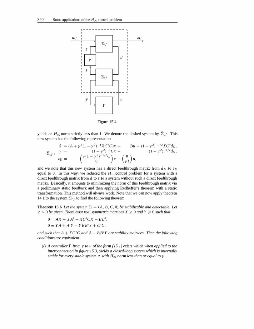
340 Some applications of theH∞ control problem
�U
� �
��
��c f
γ
�
�
�
dU zU
z
z
d
uy
Figure 15.4
yields anH∞ norm strictly less than 1. We denote the dashed system by�c f . Thisnew system has the following representation
�c f :x = (A + γ 2(1− γ 2)−1XCTC)x + Bu − (1− γ 2)−1/2XCTdU ,
y = (1− γ 2)−1Cx − (1− γ 2)−1/2dU ,
zU =(γ (1− γ 2)−1/2C
0
)x +
(0γ I
)u,
and we note that this new system has a direct feedthrough matrix fromd U to zU
equal to 0. In this way, we reduced theH∞ control problem for a system with adirect feedthrough matrix fromd to z to a system without such a direct feedthroughmatrix. Basically, it amounts to minimizing the norm of this feedthrough matrix viaa preliminary static feedback and then applying Redheffer’s theorem with a statictransformation. This method will always work. Note that we can now apply theorem14.1 to the system�c f to find the following theorem:
Theorem 15.6 Let the system � = (A, B,C,0) be stabilizable and detectable. Letγ > 0 be given. There exist real symmetric matrices X � 0 and Y � 0 such that
0= AX + X AT − XCTC X + B BT,
0= Y A + ATY − Y B BTY + CTC,
and such that A + XC TC and A − B B TY are stability matrices. Then the followingconditions are equivalent:
(i) A controller � from y to u of the form (15.1) exists which when applied to theinterconnection in figure 15.3, yields a closed-loop system which is internallystable for every stable system � with H∞ norm less than or equal to γ .
Singular problems 341
(ii) 1+ ρ(XY ) < γ−2.
Proof : The existence ofX andY follows from the results of chapter 10.
Next, we apply theorem 14.1 to the system�c f . The second algebraic Riccatiequation gets a very simple form. In fact, the question becomes whether there existsa real symmetric solutionQ � 0 to
(A − XCTC)Q + Q(A − XCTC)T − QCTC QQ = 0
such thatA − XC TC − QCTC is a stability matrix. SinceA − XC TC is stabilitymatrix, it is easy to check thatQ = 0 solves this equation. The first Riccati equationgets the following special form:
0= P A+ AT P−γ−2P B BT P+γ 2CTC+(1−γ 2)−1(γ 2I+P X)CTC(γ 2I+X P)
Via some calculations we obtain thatP = [(γ −2 − 1)I − Y X]−1Y is a stabilizingsolution of this Riccati equation. Thus, theorem 14.1 guarantees that a suitable con-troller exists for�c f if and only if P � 0, i.e. if and only if 1+ ρ(Y X) < γ −2.
Remarks:
• The existence of a suitable controller for�c f is equivalent to the existenceof a suitable controller for�c f . Hence a preliminary static output feedbackcombined with theorem 14.1 yields a suitable controller satisfying part (i)
• Our class of perturbations is rather artificial but it does not suffer from thedrawback regarding the fixed number of unstable zeros of the plant that weneeded to require for additive and multiplicative perturbations.
However, for anyλ ∈ C+, we can find a perturbation�M with ‖�M‖∞ < γ
such thatM + �M has an unstable zeroλ ∈ C+ if and only if the smallestsingular value ofM(λ) is less thanγ . Note that unstable zeros ofM +�M areequal to unstable poles of the perturbed system. The number and the locationof the unstable zeros is hence implicitly restricted by the allowed size for theperturbation�M .
• Again, we have an explicit bound for the allowable size of perturbations: part(ii) shows that for everyγ smaller than the bound[1+ρ(XY )]−1/2 we can finda suitable controller satisfying part (i).
15.3 Singular problems
In this section we shall discuss two methods which can be used to solve theH∞ pro-blem when the assumptions of theorem 14.1 are not satisfied.

342 Some applications of theH∞ control problem
15.3.1 Frequency-domain loop shifting
The basic method described in this section is based on applying a transformationsacting on transfer matrices. Consider the following transformation:
z = ε + s
1+ εswith ε > 0 then the set of alls ∈ C located outside the circle, which we denote byC⊗ε in figure 15.5 is mapped to the set of allz ∈ C in the open right half complexplaneC+. We denote the inside of the circle in figure 15.5 byC⊕.
�e
�m
−1/ε −ε
Figure 15.5
Let G be a given transfer matrix and define a new transfer matrix:
Hε(λ) = G(ε+λ1+ελ
)(15.16)
ThenG has all its poles inC⊕ε if and only if H has all its poles in the open left halfcomplex plane. AssumeG has all its poles inC⊕ε . Then
‖Hε‖∞ = supλ∈C+
‖Hε(λ)‖ = supλ∈C⊕ε
‖G(λ)‖
� supλ∈C+
‖G(λ)‖ = ‖G‖∞.
Moreover, it can be shown that:
limε↓0‖Hε‖∞ = ‖G‖∞
Moreover if G has all its poles in the open left half complex plane then there existsε∗ such thatHε has all its poles in the left half complex plane for all 0< ε < ε ∗.
Singular problems 343
What makes the transformation fromG to Hε interesting? It actually helps usrelax some of the assumptions made in our solution of theH∞ control problem:
• We needed to make assumptions that two subsystems did not have zeros on theimaginary axis. But this transformation effectively replaces the imaginary axisby the circle in figure 15.5 and by suitable choosingε we can always guaranteethat we have no zeros on the circle and therefore we can avoid this assumption.
• We needed to make assumptions that two subsystems have a direct feedthroughmatrix which is injective or surjective respectively. The points = ∞ is by ourtransformation replaces by the points = −1/ε. Now note that if a system� = (A, B,C, D) has a direct feedthrough matrix which is not injective thismight be caused by two issues:
– The system� has a transfer matrixG which is not injective as a rationalmatrix, i.e. rankG(s) is less than the number of columns ofG for alls ∈ C.
– The system� has an infinite zero.
Our transformation can avoid the assumption that� has no infinite zeros be-cause it replacess = ∞ by the points = −1/ε. However if the transfer matrixis not injective as a rational matrix then this transformation does not help us inremoving this assumption.
There are many other similar transformations based on transfer matrices that wecan use. For instancez = s + ε which moves the imaginary axis to the line�es =−ε. The reason why the transformation described by (15.16) is popular is that itavoids that the closed loop system has poles close to the imaginary axis with a largeimaginary part. These yield very fast oscillations in the closed loop system which arevery badly damped and are highly undesirable in applications.
Let us next describe how we will use this transformation. Suppose we have asystem of the form:
� :x = Ax + Bu + Ed,y = C1x + D11u + D12d,z = C2x + D21u + D22d,
(15.17)
with transfer matrixG from (u, d) to (y, z). If I − εA is invertible we can define thefollowing transformed system:
�ε :x = Ax + Bu + Ed,y = C1x + D11u + D12d,z = C2x + D21u + D22d,
(15.18)
344 Some applications of theH∞ control problem
where
A : = (A − ε I )(I − εA)−1,
B : = (1− ε2)(I − εA)−1B,
E : = (1− ε2)(I − εA)−1E,
C1 : = C1(I − εA)−1,
C2 : = C2(I − εA)−1,
D11 : = D11+ εC1(I − εA)−1B,
D12 : = D12+ εC1(I − εA)−1E,
D21 : = D21+ εC2(I − εA)−1B,
D22 : = D22+ εC2(I − εA)−1E .
Note that the transfer matrix of this transformed system is given by:
Gε(λ) = G(ε+λ1+ελ
)In other words, we basically applied exactly the transformation as described before.
Assume that a controller� described by the transfer matrix� exists for�ε suchthat the closed-loop system is internally stable and the closed-loop transfer matrixGcl has H∞ norm less than 1. Then if we apply the feedback� described by thetransfer matrixH where
H (λ) = H
(ε − λελ− 1
)
to our original system, then the closed-loop system� ×�, with transfer matrixG cl ,is related to the closed-loop system�ε × �, with transfer matrixGcl , via the abovetransformation, i.e.
Gcl(λ) = Gcl
(ε + λ1+ ελ
).
Moreover, it can be shown that the state matrix of the closed-loop system� × � hasall its eigenvalues insideC⊕ε . Hence the closed-loop system is certainly internallystable. Using the same arguments as before, we have
‖Gcl‖∞ � ‖Gcl‖∞.Hence if� applied to�ε makes theH∞ norm less than some boundγ , then� makesthe H∞ norm of the closed-loop transfer matrixG cl also less thanγ .
On the other hand, if, for the system�, there is a stabilizing static controller�which makes theH∞ norm of the closed-loop system strictly less thanγ then it canbe shown that there existsε1 > 0 such that for all 0< ε � ε1 the transformedsystem�ε with the transformed controller� is internally stable and theH∞ norm ofthe closed-loop system is strictly less thanγ .
Singular problems 345
Now for all but finitely manyε > 0 the system�ε, described by (15.18) is suchthat the systems( A, B, C2, D21) and( A, E, C1, D12) have no zeros on the imaginaryaxis. However,D21 and D12 will not always be injective and surjective respectively.Either they are injective and surjective for all but finitely manyε, or they are notfor any value ofε. This is in line with what we noted before as the advantages ofthis transformation. The matricesD11 and D22 will be there and therefore we cannot directly apply theorem 14.1. But we have described methods to get rid of thesematrices in the previous section.
Therefore, to check if for� there is an internally stabilizing feedback controllerwhich makes theH∞ norm of the closed-loop system less thanγ we can, in mostcases, use theorem 14.1. Note that we have to check the conditions of theorem 14.1for someε > 0. The problem is that we do not know how small we must makeε. Iffor someε > 0 the conditions of theorem 14.1 are satisfied, then we find a suitablecontroller. However, if the conditions of theorem 14.1 are not satisfied then either nosuitable controller exists, or one does exist in which case the conditions of theorem14.1 are satisfied for some smallerε. Therefore we are never sure. Moreover, forsmallε we very easily run into numerical difficulties.
15.3.2 Cheap control
In the previous section we described an approach to solve theH∞ control problemif we have zeros on the imaginary axis or assumptions on the direct feedthroughmatrices are not satisfied. This extends theorem 14.1 which can only be used if theseassumptions are satisfied. In this subsection we shall briefly describe an alternativeapproach.
Assume that we have a system� of the form
� :x = Ax + Bu + Ed,y = C1x + D1d,z = C2x + D2u.
(15.19)
For eachε > 0 we define the following perturbed system:
�ε :x = Ax + Bu + Ed,y = C1x + D1d,z = C2x + D2u,
(15.20)
where
C2 =C2ε I0
, D2 =
D2
0ε I
, E = (
E ε I 0), D1 =
(D1 0 ε I
).
The structure of the perturbations on the matrices is such that it is easy to show thatany controller� of the form (15.1) has the property that� is internally stabilizingwhen applied to� if and only if the same controller� is internally stabilizing whenapplied to�ε. Actually the closed loop poles of these two systems coincide.
346 Some applications of theH∞ control problem
Let � be internally stabilizing when applied to�. Denote the closed-loop oper-ator mappingw to z with zero initial state byGcl . Moreover, denote the closed-loopoperator mappingw to z with zero initial state when the controller is applied to�εby Gcl,ε . Then we have
‖Gcl‖∞ � ‖Gcl,ε1‖∞ � ‖Gcl,ε2‖∞for all 0 � ε1 � ε2. Hence, if we have an internally stabilizing controller whichmakes theH∞ norm of the closed-loop system less thanγ when applied to the system�ε, then the same controller is internally stabilizing and makes theH∞ norm of theclosed-loop system less thanγ when applied to the original system. Thus we obtainthe following result:
Theorem 15.7 Let a system � be given by (15.19). For all ε > 0 define �ε by(15.20). The following two statements are equivalent:
(i) For the system � there is a feedback � of the form (15.1) which is internallystabilizing and which makes the H∞ norm of the closed-loop system less than1.
(ii) There exists ε1 > 0 such that for all 0 < ε < ε1 there is a feedback � ofthe form (15.1) for �ε which is internally stabilizing and which makes theH∞ norm of the closed-loop system less than 1.
Any controller satisfying part (ii) for some ε > 0 also satisfies part (i).
On the other hand, for the system�ε the subsystems (A, B, C2, D2) and (A, E ,C1, D1) do not have zeros and hence certainly no zeros on the imaginary axis. More-over, D1 and D2 are surjective and injective, respectively. Hence, we may apply theresults of theorem 14.1 to the system�(ε) to obtain necessary and sufficient condi-tions for the existence of internally stabilizing controllers which make theH∞ normof the closed-loop system less than 1.
If we compare the method of the previous subsection with the method of thecurrent subsection, then we see that the method of this subsection is much easier.First of all, we do not have to apply transformations on the controller. Secondly,for all ε > 0 the system (15.20) is proper and satisfies the assumptions of chapter13. In contrast, for some values ofε > 0, the system (15.18) is either not proper orthe conditions of theorem 14.1 are not satisfied. Finally, the method of the previoussubsection might yield systems which do not satisfy the assumptions of theorem 14.1for any value ofε.
Both methods have the disadvantage that the conditions cannot actually be check-ed since the conditions in the previous subsection as well as the conditions in thissubsection have to be checked for an infinite number ofε > 0.
One of the main reasons for using the method of the previous subsection is be-cause all closed-loop poles will be placed inside a circle in the open left half complexplane and therefore the closed-loop system will not have ill-damped high-frequencypoles.
The minimum entropyH∞ control problem 347
15.4 The minimum entropy H∞ control problem
We have been studying theH∞ control problem. InH∞ control we design controllersto minimize the peak value of the largest singular value of the transfer matrix on theimaginary axis. It can be shown that (near)optimal controllers have a flat magnitudeBode diagram. On the other hand for the classicalH2 or Linear Quadratic Gaussian(LQG) control problem (see chapter 11) the average value of the transfer matrix overthe imaginary axis is minimized. The latter problem is not concerned with peaks aslong as they have small width.
The above reasoning implies thatH∞ control is well-suited for robustness syn-thesis via the small-gain theorem. On the other hand, robust controllers might leadto a large closed loopH2 norm. This motivates a new synthesis problem: minimizethe H2 norm under anH∞ norm bound. It is hoped that theH∞ norm bound yieldsthe desired level of robustness while performance is optimized simultaneously via theminimization of theH2 norm.
The minimum entropyH∞ control problem is defined as the problem of minimiz-ing an entropy function under the constraint of internal stability of the closed-loopsystem and under the constraint of an upper bound on theH∞ norm of the closed-looptransfer matrix. It is a mixture between optimizing theH∞ norm and theH2 norm. Itis also yields a better understanding of why the controllers we obtained in theorems13.3 and 14.1 converge to theH2 controllers from chapter 10. Therefore, it is hopedthat by minimizing this entropy function, one can obtain a good trade-off between theH∞ norm for robustness and theH2 norm for performance.
15.4.1 Problem formulation and results
Consider the linear time-invariant system:
� :x = Ax + Bu + Ed,y = C1x + D1d,z = C2x + D1u.
(15.21)
Here,A, B, E,C1,C2, D1 andD2 are real matrices of suitable dimension. LetG bea strictly proper real rational matrix which has no poles on the imaginary axis andwhich is such that‖G‖∞ < γ . For such a transfer matrixG, we define the followingentropy function:
Jγ (G) : = − γ2
2π
∫ ∞
−∞ln det
(I − γ−2G∼(iω)G(iω)
)dω (15.22)
whereG∼(s) : = GT(−s). The minimum entropyH∞ control problem is then definedas:
Minimize Jγ (Gcl) over all controllers which yield a strictly proper, in-ternally stable closed-loop transfer matrixG cl with H∞ norm strictly lessthanγ .
348 Some applications of theH∞ control problem
We shall investigate controllers of the form (15.1). We can now formulate themain result of this chapter:
Theorem 15.8 Consider the system (15.21). Assume that the systems (A, B,C2, D2)
and (A, E,C1, D1) have no zeros on the imaginary axis, with D1 and D2 surjectiveand injective, respectively. Assume that a controller exists which is such that theclosed-loop system is internally stable and has H∞ norm strictly less than γ . Theinfimum of J(Gcl), over all internally stabilizing controllers of the form (15.1) whichare such that the closed system has H∞ norm strictly less than γ , is equal to:
trace[ET P E
]+ trace[(AT P + P A + CT
2C2 + γ−2P E E T P)(I − γ−2Q P)−1Q]
where P and Q are such that part (ii) of theorem 14.1 is satisfied, and G cl denotesthe closed loop transfer matrix. The infimum is attained by the controller given intheorem 14.1.
15.4.2 Properties of the entropy function
In this section we recall some basic properties of the entropy function as defined in(15.22). Note that in order to prove some of the results in this section some a prioriknowledge of function theory is required. Those students not familiar with this areacan skip the proofs in this section.
Lemma 15.9 Let G be a strictly proper, stable rational matrix such that ‖G‖∞ � γ .Then we have
• Jγ (G) � 0 and Jγ (G) = 0 implies G = 0,
• Jγ (G) = Jγ (GT).
Next, we relate our entropy function to theH2 norm studied in chapter 10. Wefind:
Lemma 15.10 Let a system � = (A, B,C,0) be such that A is stable. Let G bethe transfer matrix of �. We have Jγ (G) � ‖G‖2
2. Moreover, Jγ (G) → ‖G‖22 as
γ →∞.
Proof : For an arbitrary symmetric matrixA we have
− ln det(I − A) = − ln(1− λi ) = −� ln(1− λi ) � � − λi = − trace[A]whereλi denote the eigenvalues ofA. This immediately yields the first inequality:
− γ2
2π
∫ ∞
−∞ln det
(I − γ−2G∼(iω)G(iω)
)dω � 1
2π
∫ ∞
−∞traceG∼(iω)G(iω) dω
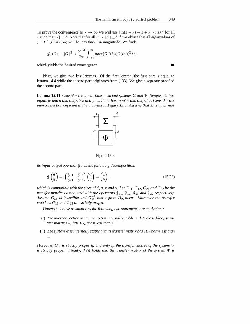
The minimum entropyH∞ control problem 349
To prove the convergence asγ →∞ we will use| ln(1− λ) − 1+ λ| < ελ2 for allλ such that|λ| < δ. Note that for allγ > ‖G‖∞δ−1 we obtain that all eigenvalues ofγ−2G∼(iω)G(iω) will be less thanδ in magnitude. We find:
Jγ (G)− ‖G‖2 <γ−2
2π
∫ ∞
−∞trace[G∼(iω)G(iω)]2 dω
which yields the desired convergence.
Next, we give two key lemmas. Of the first lemma, the first part is equal tolemma 14.4 while the second part originates from [133]. We give a separate proof ofthe second part.
Lemma 15.11 Consider the linear time-invariant systems � and � . Suppose � hasinputs w and u and outputs z and y, while � has input y and output u. Consider theinterconnection depicted in the diagram in Figure 15.6. Assume that � is inner and
�
��
�
�
�
y
z d
u
Figure 15.6
its input-output operator G has the following decomposition:
G
(du
)=:
(G11 G12G21 G22
)(du
)=
(zy
), (15.23)
which is compatible with the sizes of d, u, z and y. Let G 11, G12, G21 and G22 be thetransfer matrices associated with the operators G11, G12, G21 and G22 respectively.Assume G21 is invertible and G−1
21 has a finite H∞ norm. Moreover the transfermatrices G11 and G22 are strictly proper.
Under the above assumptions the following two statements are equivalent:
(i) The interconnection in Figure 15.6 is internally stable and its closed-loop tran-sfer matrix Gcl has H∞ norm less than 1.
(ii) The system� is internally stable and its transfer matrix has H∞ norm less than1.
Moreover, Gcl is strictly proper if, and only if, the transfer matrix of the system �
is strictly proper. Finally, if (i) holds and the transfer matrix of the system � is
350 Some applications of theH∞ control problem
strictly proper then the following relation between the entropy functions for the dif-ferent transfer matrices is satisfied:
J1(Gcl) = J1(G11)+ J1(Q). (15.24)
Proof : The first claim that the statements (i) and (ii) are equivalent, has been shownin lemma 14.4. We know thatG 11 andG22 are strictly proper. Combined with thefact that� is inner, this implies thatG12 andG21 are bicausal, i.e. they are invertibleand both the transfer matrices and their inverses are proper. Using this, it is easy tocheck that the transfer matrixH of � is strictly proper if and only ifG cl is strictlyproper.
We still have to prove equation (15.24). The following equality is easily de-rived using the property that� is inner (in particular that its transfer matrix satisfiesGT(s)G(s) = I ).
I − G∼cl Gcl = G∼21
(I − H∼G∼22
)−1(
I − H∼H)(I − G22H )−1 G21.
Therefore, we find that
ln det(I − G∼cl Gcl
)= ln det
(I − G∼11G11
) + ln det(I − H∼H
)− 2 ln det(I − G22H ) .
Moreover, if statement (i) is satisfied and ifH is strictly proper then we have
J1(H ) = − 1
2π
∫ ∞
−∞ln det
(I − H∼(iω)H (iω)
)dω, (15.25)
J1(G11) = − 1
2π
∫ ∞
−∞ln det
(I − G∼11(iω)G11(iω)
)dω. (15.26)
Using the fact thatH is strictly proper, stable and hasH∞ norm strictly less than 1and the fact thatG22 is also stable, strictly proper and hasH∞ norm less than or equalto 1, we know that ln det(I − G22(λ)H (λ)) is an analytic function in the open righthalf plane and that a constantM exists such that
| ln det(I − G22(λ)Q(λ)) | < M
|λ|2 , ∀λ ∈ C0 ∪ C+
This implies, using Cauchy’s theorem, that∫ ∞
−∞ln det(I − G22(iω)Q(iω)) dω = 0 (15.27)
Combining the above, we find (15.24).
The following lemma is an essential tool for actually calculating the entropy func-tion for some specific system:
The minimum entropyH∞ control problem 351
Lemma 15.12 Let � = (A, B,C, D) be stabilizable and detectable with transfermatrix G ans with detD = 1. Also, assume that G,G−1 ∈ H∞ and G has H∞ normequal to 1. Then we have:∫ ∞
−∞ln | detG(iω)| dω = −π trace[B D−1C]. (15.28)
Proof : Denote the integral in (15.28) byK and define
a : = − traceB D−1C.
We have (remember that ln|z| = �e lnz):
K = �e
(∫ ∞
−∞ln detG(iω)− a
1+ iωdω
)+ a
∫ ∞
−∞dω
1+ ω2(15.29)
Next, it is easily checked thatp(s) : = ln detG(s)− a1+s is a bounded analytic func-
tion in C+ such thatp(s) = O(1/s2) (|s| → ∞, Res � 0). Hence, using Cauchy’stheorem we find∫ ∞
−∞p(iω) dω = 0. (15.30)
Combining (15.29) and (15.30) yields (15.28).
Corollary 15.13 Let� = (A, B,C,0) be internally stable with strictly proper trans-fer matrix G. Assume G has H∞ norm strictly less than γ . Then we have:
Jγ (G) = traceBT X B, (15.31)
where X is the unique reak symmetric solution of the algebraic Riccati equation:
X A + AT X + γ−2X B BT X + CTC = 0,
such that A + γ −2B BT X is asymptotically stable.
Proof : The existence and uniqueness ofX is a consequence of the bounded reallemma (see section 12.6). It is easy to check that the transfer matrixM with realiza-tion (A, B,−γ−2BT X, I ) satisfies:
I − γ−2G∼G = M∼M.
Moreover,M,M−1 ∈ H∞, i.e. M is a spectral factor ofI − γ −2G∼G. We have
Jγ (G) = −γ2
π
∫ ∞
−∞ln | detM(iω)| dω,
and therefore (15.31) is a direct consequence of applying lemma 15.12 to the aboveequation.
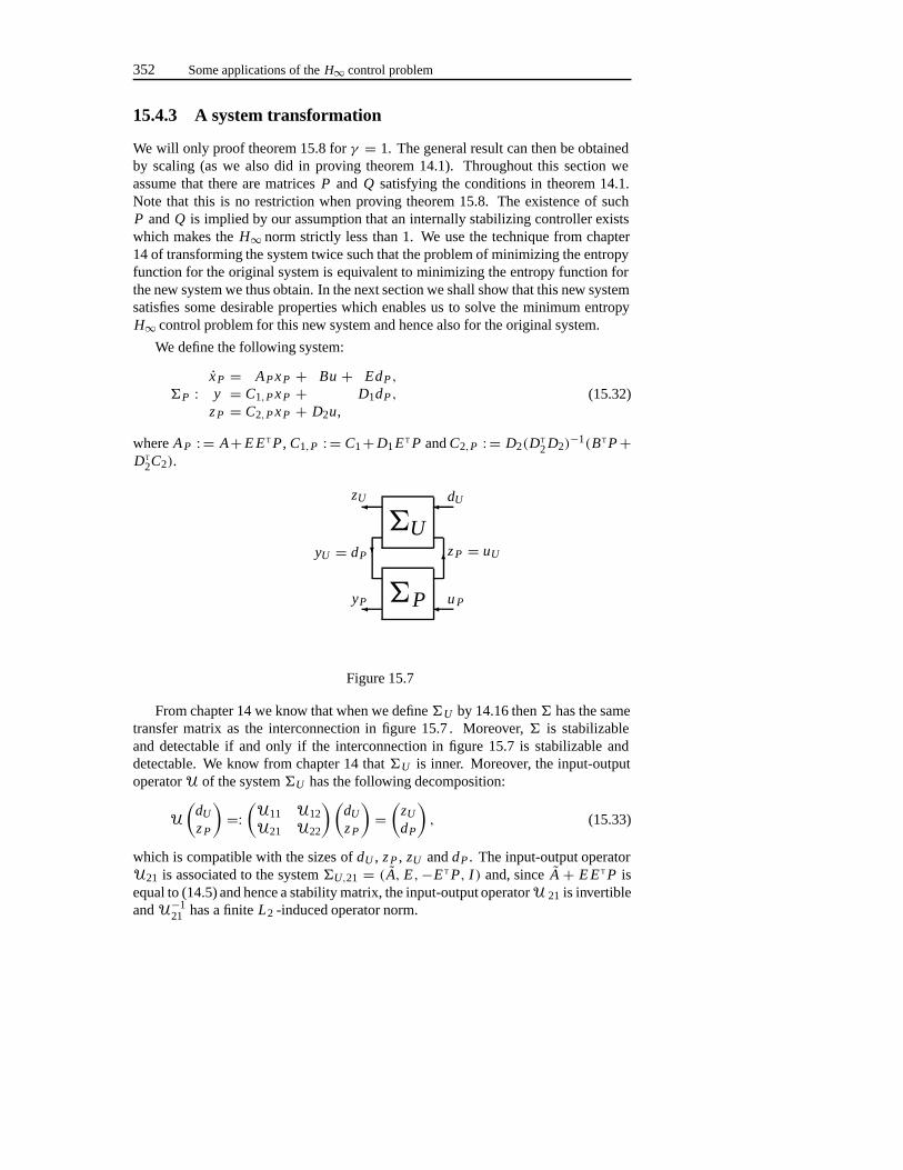
352 Some applications of theH∞ control problem
15.4.3 A system transformation
We will only proof theorem 15.8 forγ = 1. The general result can then be obtainedby scaling (as we also did in proving theorem 14.1). Throughout this section weassume that there are matricesP and Q satisfying the conditions in theorem 14.1.Note that this is no restriction when proving theorem 15.8. The existence of suchP andQ is implied by our assumption that an internally stabilizing controller existswhich makes theH∞ norm strictly less than 1. We use the technique from chapter14 of transforming the system twice such that the problem of minimizing the entropyfunction for the original system is equivalent to minimizing the entropy function forthe new system we thus obtain. In the next section we shall show that this new systemsatisfies some desirable properties which enables us to solve the minimum entropyH∞ control problem for this new system and hence also for the original system.
We define the following system:
�P :x P = AP x P + Bu + EdP ,
y = C1,P x P + D1dP ,
z P = C2,P x P + D2u,(15.32)
whereA P : = A+E E T P, C1,P : = C1+D1ET P andC2,P : = D2(DT
2D2)−1(BT P+
DT
2C2).
�P
�U
�yP
�
�u P
�
��
zU dU
yU = dP z P = uU
Figure 15.7
From chapter 14 we know that when we define�U by 14.16 then� has the sametransfer matrix as the interconnection in figure 15.7 . Moreover,� is stabilizableand detectable if and only if the interconnection in figure 15.7 is stabilizable anddetectable. We know from chapter 14 that�U is inner. Moreover, the input-outputoperatorU of the system�U has the following decomposition:
U
(dU
z P
)=:
(U11 U12U21 U22
)(dU
z P
)=
(zU
dP
), (15.33)
which is compatible with the sizes ofdU , z P , zU anddP . The input-output operatorU21 is associated to the system�U,21 = ( A, E,−E T P, I ) and, sinceA + E E T P isequal to (14.5) and hence a stability matrix, the input-output operatorU 21 is invertibleandU−1
21 has a finiteL2 -induced operator norm.
The minimum entropyH∞ control problem 353
Moreover, by corollary 15.13, we haveJ1(U11) = traceE T P E . Combining theabove with lemma 15.11, we find the following theorem:
Theorem 15.14Let the systems (15.21) and (15.32) be given. Moreover, let a con-troller � of the form (15.1) be given. The following two conditions are equivalent:
• � is internally stabilizing for � such that the closed-loop transfer matrix G cl
is strictly proper and has H∞ norm strictly less than 1.
• � is internally stabilizing for �P such that the closed-loop transfer matrixGcl,P is strictly proper and has H∞ norm strictly less than 1.
Moreover, if � satisfies the above conditions then we have
J1(Gcl) = J1(Gcl,P )+ traceE T P E .
Next, we make another transformation from� P to�P,Q . This transformation isexactly dual to the transformation from� to� P . We know there exists a controllerwhich is internally stabilizing for�P which makes theH∞ norm of the closed-loopsystem strictly less than 1. Therefore if we apply lemma 14.8 together with theorem14.1 to�P we find that the matrixY = (I − Q P)−1Q is a real symmetric solutionof (14.19) such that (14.21) is a stability matrix. We define the following system:
�P,Q :x P,Q = AP,Q x P,Q + BP,Qu + E P,Qd,
y = C1,P x P,Q + D1dP,Q,
z P,Q = C2,P x P,Q + D2u,(15.34)
where
AP,Q : = AP + Y CT
2,PC2,P ,
BP,Q : = B + Y CT
2,P D2,
E P,Q : = (Y CT
1,P + E DT
1)(D1DT
1)−1D1.
Using theorem 15.14 and a dualized version for the transformation from� P to�P,Q we can derive the following corollary:
Corollary 15.15 Let the systems (15.21) and (15.34) be given. Moreover, let a con-troller � of the form (15.1) be given. The following two conditions are equivalent:
• � is internally stabilizing for � such that the closed-loop transfer matrix G cl
is strictly proper and has H∞ norm strictly less than 1.
• � is internally stabilizing for �P,Q such that the closed-loop transfer matrixGcl,P,Q is strictly proper and has H∞ norm strictly less than 1.
Moreover, if � satisfies the above conditions then we have
J1(Gcl) = J1(Gcl,P,Q )+ traceE T P E + traceC1,PY C1,P .
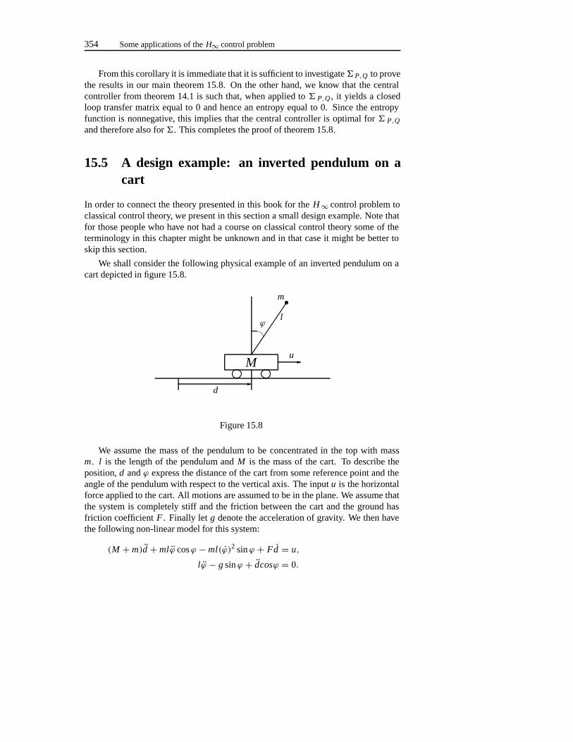
354 Some applications of theH∞ control problem
From this corollary it is immediate that it is sufficient to investigate� P,Q to provethe results in our main theorem 15.8. On the other hand, we know that the centralcontroller from theorem 14.1 is such that, when applied to� P,Q , it yields a closedloop transfer matrix equal to 0 and hence an entropy equal to 0. Since the entropyfunction is nonnegative, this implies that the central controller is optimal for� P,Q
and therefore also for�. This completes the proof of theorem 15.8.
15.5 A design example: an inverted pendulum on acart
In order to connect the theory presented in this book for theH∞ control problem toclassical control theory, we present in this section a small design example. Note thatfor those people who have not had a course on classical control theory some of theterminology in this chapter might be unknown and in that case it might be better toskip this section.
We shall consider the following physical example of an inverted pendulum on acart depicted in figure 15.8.
M �
�
ϕ
m
l
u
d
Figure 15.8
We assume the mass of the pendulum to be concentrated in the top with massm. l is the length of the pendulum andM is the mass of the cart. To describe theposition,d andϕ express the distance of the cart from some reference point and theangle of the pendulum with respect to the vertical axis. The inputu is the horizontalforce applied to the cart. All motions are assumed to be in the plane. We assume thatthe system is completely stiff and the friction between the cart and the ground hasfriction coefficientF . Finally let g denote the acceleration of gravity. We then havethe following non-linear model for this system:
(M + m)d + mlϕ cosϕ − ml(ϕ)2 sinϕ + Fd = u,
lϕ − g sinϕ + dcosϕ = 0.
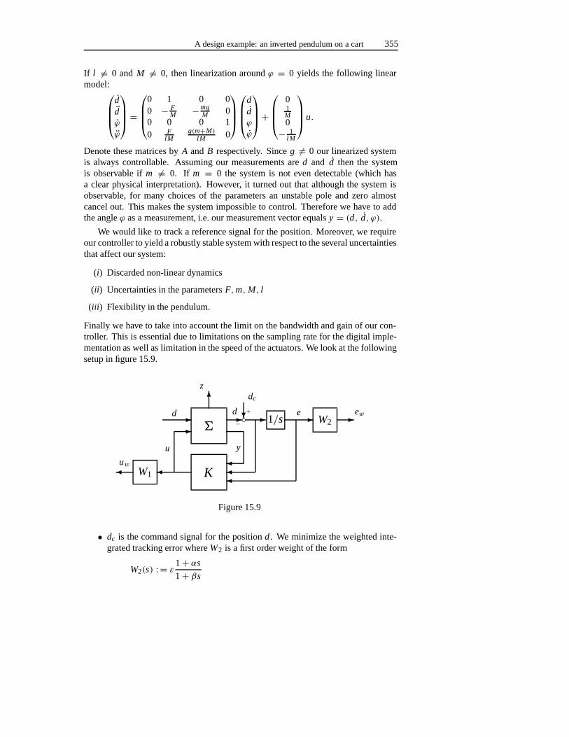
A design example: an inverted pendulum on a cart 355
If l = 0 andM = 0, then linearization aroundϕ = 0 yields the following linearmodel:
ddϕ
ϕ
=
0 1 0 00 − F
M −mgM 0
0 0 0 10 F
lMg(m+M)
lM 0
ddϕ
ϕ
+
01M0− 1
lM
u.
Denote these matrices byA and B respectively. Sinceg = 0 our linearized systemis always controllable. Assuming our measurements ared and d then the systemis observable ifm = 0. If m = 0 the system is not even detectable (which hasa clear physical interpretation). However, it turned out that although the system isobservable, for many choices of the parameters an unstable pole and zero almostcancel out. This makes the system impossible to control. Therefore we have to addthe angleϕ as a measurement, i.e. our measurement vector equalsy = (d, d, ϕ).
We would like to track a reference signal for the position. Moreover, we requireour controller to yield a robustly stable system with respect to the several uncertaintiesthat affect our system:
(i) Discarded non-linear dynamics
(ii) Uncertainties in the parametersF,m,M, l
(iii) Flexibility in the pendulum.
Finally we have to take into account the limit on the bandwidth and gain of our con-troller. This is essential due to limitations on the sampling rate for the digital imple-mentation as well as limitation in the speed of the actuators. We look at the followingsetup in figure 15.9.
W1 K
�1/s W2
� �
��
�
�
���
� � ��
uw
d
z
d
dc
e
u y
ew◦−+
Figure 15.9
• dc is the command signal for the positiond. We minimize the weighted inte-grated tracking error whereW2 is a first order weight of the form
W2(s) : = ε1+ αs
1+ βs
356 Some applications of theH∞ control problem
By choosingα << β we obtain a low pass filter. This expresses that we areonly interested in tracking low-frequency signals. The integrator also expressesour interest in low frequencies: it is one way to guarantee zero steady statetracking error. Finallyε in the weight is used to express the relative importanceof tracking over the other goals we have for the system.
• We also minimizeuw which is the weighted control input.W1 has the samestructure asW2. However, this time we chooseα >> β to obtain a high passfilter. We would like to constrain the open-loop bandwidth and gain of the con-troller. This facilitates digital implementation and it also prevents us pushingour actuators beyond their capabilities. Finally, it prevents the controller stim-ulating high-frequency uncertainty in the system dynamics, such as bendingmodes of the pendulum. Since we cannot incorporate open-loop limitationsdirectly in anH∞ design, we push the bandwidth and gain down indirectly viathis weight onu. However, it turned out to be very hard to make the bandwidthsmall.
• z andd are new inputs and outputs we add to the system� to express robust-ness requirements, i.e. the system� is of the form:
� :
x = Ax + Bu + Ed,
y =1 0 0 0
0 1 0 00 0 1 0
x ,
z = C2x .
(15.35)
The matricesA andB are as defined before. On the other hand,E andC 2 stillhave to be chosen. For instance if we want to guard against fluctuations in theparametersF andm, the friction and the mass of the pendulum, then we chooseE andC2 as:
E : =
0−1/M
01/ l M
, C2 : =
(0 1 0 00 0 g 0
). (15.36)
This amounts to a�-block such as depicted in (12.3) where� = (Fr−F mr−m). An H∞ norm less thanγ from d to z then guarantees that if the trueparameter valuesFr ,mr differ from the nominal valuesm, r less thanγ −1 (tobe precise such that‖�‖ � γ −1), the system will still be stable. A similardefinition can be made to guard against fluctuations in all parameters of the 2differential equations due to discarded non-linearities or flexibility of the beam.In that case we choose, instead of (15.36),E andC 2 as:
E : =
0 01 00 00 1
, C2 : =
1 0 0 00 1 0 00 0 1 00 0 0 1
. (15.37)
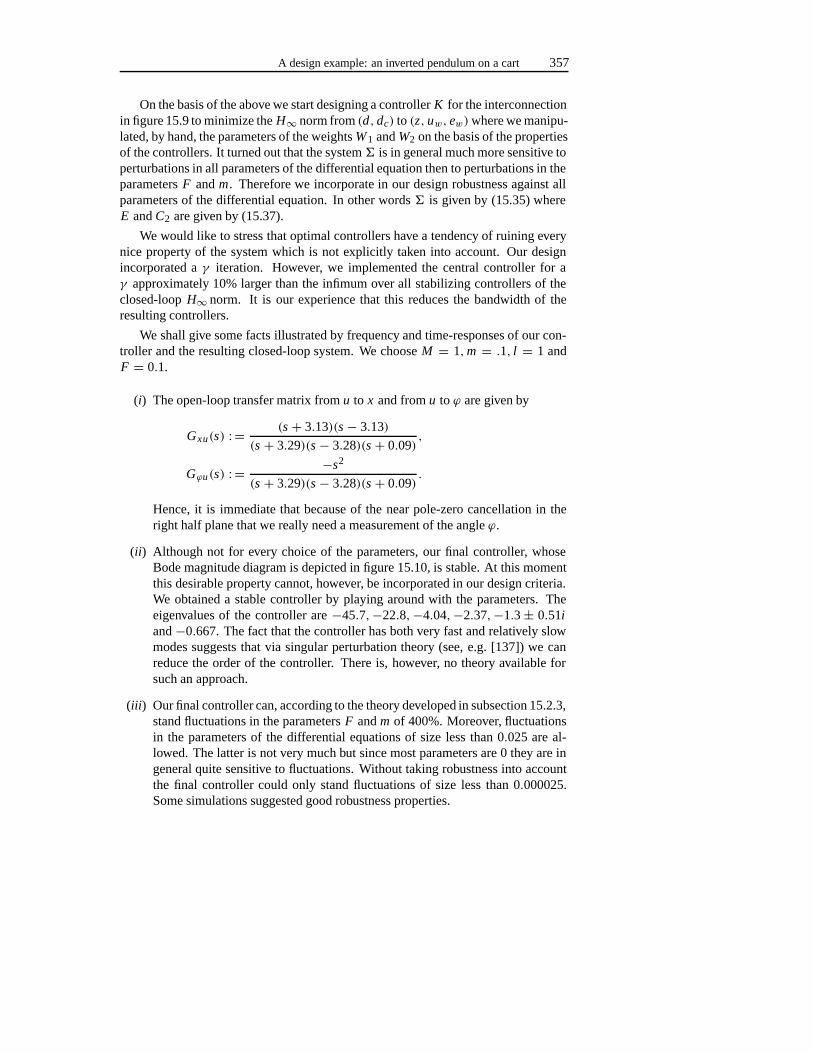
A design example: an inverted pendulum on a cart 357
On the basis of the above we start designing a controllerK for the interconnectionin figure 15.9 to minimize theH∞ norm from(d, dc) to (z, uw, ew)where we manipu-lated, by hand, the parameters of the weightsW1 andW2 on the basis of the propertiesof the controllers. It turned out that the system� is in general much more sensitive toperturbations in all parameters of the differential equation then to perturbations in theparametersF andm. Therefore we incorporate in our design robustness against allparameters of the differential equation. In other words� is given by (15.35) whereE andC2 are given by (15.37).
We would like to stress that optimal controllers have a tendency of ruining everynice property of the system which is not explicitly taken into account. Our designincorporated aγ iteration. However, we implemented the central controller for aγ approximately 10% larger than the infimum over all stabilizing controllers of theclosed-loopH∞ norm. It is our experience that this reduces the bandwidth of theresulting controllers.
We shall give some facts illustrated by frequency and time-responses of our con-troller and the resulting closed-loop system. We chooseM = 1,m = .1, l = 1 andF = 0.1.
(i) The open-loop transfer matrix fromu to x and fromu to ϕ are given by
Gxu(s) : = (s + 3.13)(s − 3.13)
(s + 3.29)(s − 3.28)(s + 0.09),
Gϕu(s) : = −s2
(s + 3.29)(s − 3.28)(s + 0.09).
Hence, it is immediate that because of the near pole-zero cancellation in theright half plane that we really need a measurement of the angleϕ.
(ii) Although not for every choice of the parameters, our final controller, whoseBode magnitude diagram is depicted in figure 15.10, is stable. At this momentthis desirable property cannot, however, be incorporated in our design criteria.We obtained a stable controller by playing around with the parameters. Theeigenvalues of the controller are−45.7,−22.8,−4.04,−2.37,−1.3± 0.51iand−0.667. The fact that the controller has both very fast and relatively slowmodes suggests that via singular perturbation theory (see, e.g. [137]) we canreduce the order of the controller. There is, however, no theory available forsuch an approach.
(iii) Our final controller can, according to the theory developed in subsection 15.2.3,stand fluctuations in the parametersF andm of 400%. Moreover, fluctuationsin the parameters of the differential equations of size less than 0.025 are al-lowed. The latter is not very much but since most parameters are 0 they are ingeneral quite sensitive to fluctuations. Without taking robustness into accountthe final controller could only stand fluctuations of size less than 0.000025.Some simulations suggested good robustness properties.
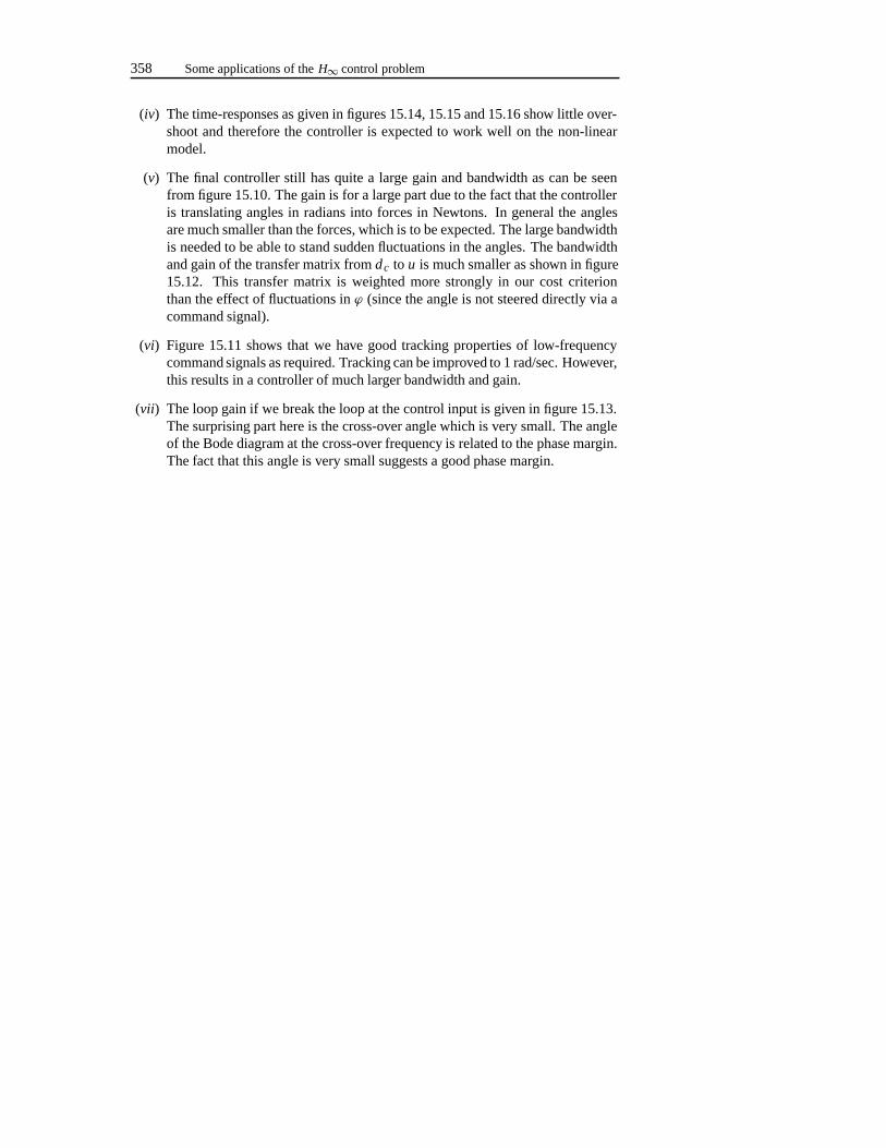
358 Some applications of theH∞ control problem
(iv) The time-responses as given in figures 15.14, 15.15 and 15.16 show little over-shoot and therefore the controller is expected to work well on the non-linearmodel.
(v) The final controller still has quite a large gain and bandwidth as can be seenfrom figure 15.10. The gain is for a large part due to the fact that the controlleris translating angles in radians into forces in Newtons. In general the anglesare much smaller than the forces, which is to be expected. The large bandwidthis needed to be able to stand sudden fluctuations in the angles. The bandwidthand gain of the transfer matrix fromdc to u is much smaller as shown in figure15.12. This transfer matrix is weighted more strongly in our cost criterionthan the effect of fluctuations inϕ (since the angle is not steered directly via acommand signal).
(vi) Figure 15.11 shows that we have good tracking properties of low-frequencycommand signals as required. Tracking can be improved to 1 rad/sec. However,this results in a controller of much larger bandwidth and gain.
(vii) The loop gain if we break the loop at the control input is given in figure 15.13.The surprising part here is the cross-over angle which is very small. The angleof the Bode diagram at the cross-over frequency is related to the phase margin.The fact that this angle is very small suggests a good phase margin.
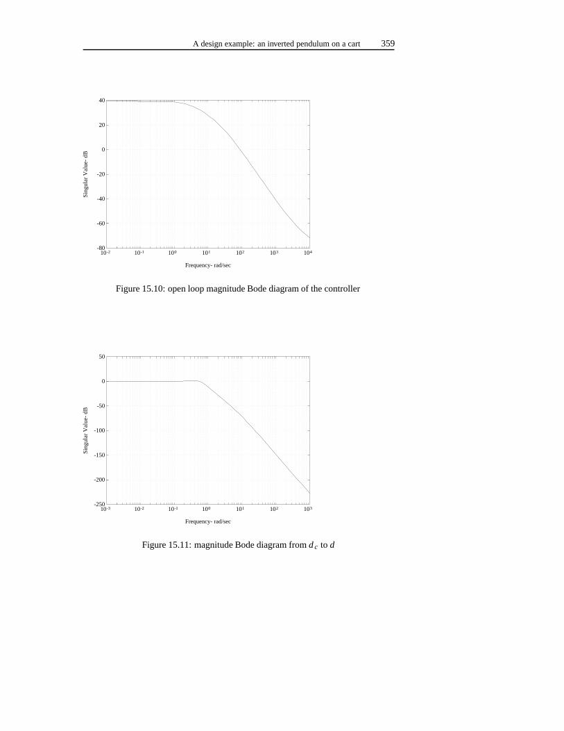
A design example: an inverted pendulum on a cart 359
-80
-60
-40
-20
0
20
40
10-2 10-1 100 101 102 103 104
Frequency- rad/sec
Sin
gula
r V
alue
- dB
Figure 15.10: open loop magnitude Bode diagram of the controller
-250
-200
-150
-100
-50
0
50
10-3 10-2 10-1 100 101 102 103
Frequency- rad/sec
Sin
gula
r V
alue
- dB
Figure 15.11: magnitude Bode diagram fromd c to d
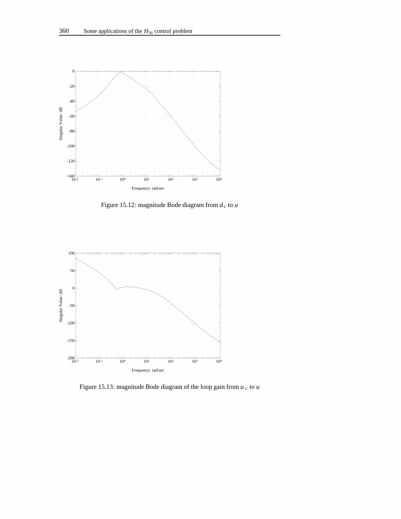
360 Some applications of theH∞ control problem
-140
-120
-100
-80
-60
-40
-20
0
10-2 10-1 100 101 102 103 104
Frequency- rad/sec
Sin
gula
r V
alue
- dB
Figure 15.12: magnitude Bode diagram fromd c to u
-200
-150
-100
-50
0
50
100
10-2 10-1 100 101 102 103 104
Frequency- rad/sec
Sin
gula
r V
alue
- dB
Figure 15.13: magnitude Bode diagram of the loop gain fromu c to u
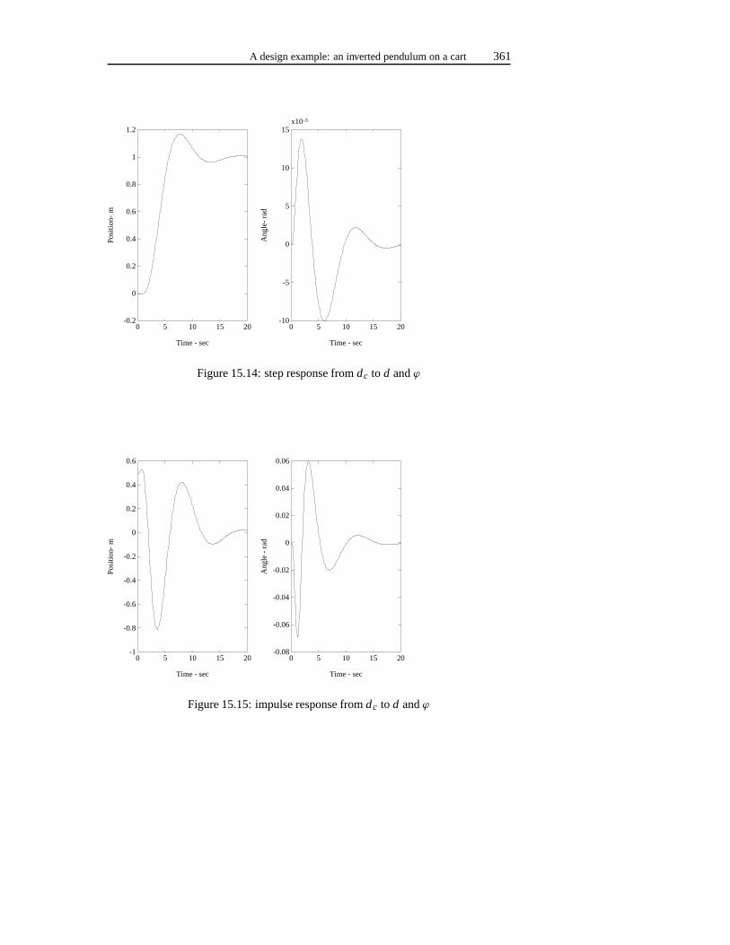
A design example: an inverted pendulum on a cart 361
-0.2
0
0.2
0.4
0.6
0.8
1
1.2
0 5 10 15 20
Time - sec
Pos
ition
- m
-10
-5
0
5
10
15x10-3
0 5 10 15 20
Time - sec
Ang
le-
rad
Figure 15.14: step response fromdc to d andϕ
-1
-0.8
-0.6
-0.4
-0.2
0
0.2
0.4
0.6
0 5 10 15 20
Time - sec
Pos
ition
- m
-0.08
-0.06
-0.04
-0.02
0
0.02
0.04
0.06
0 5 10 15 20
Time - sec
Ang
le -
rad
Figure 15.15: impulse response fromdc to d andϕ
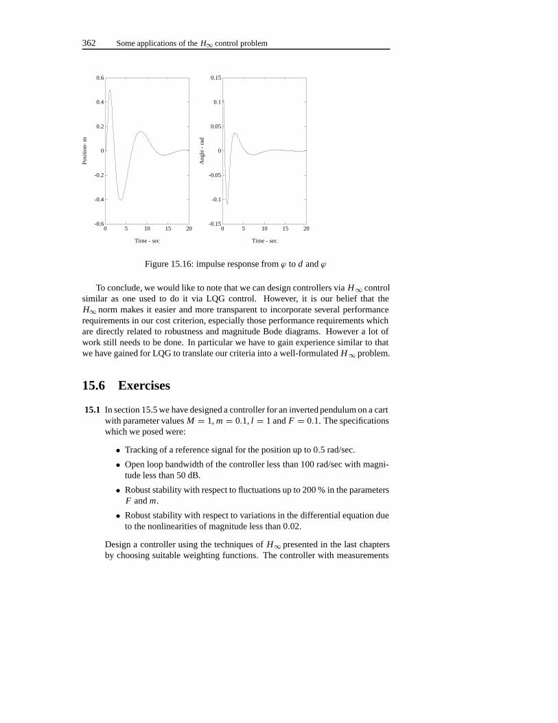
362 Some applications of theH∞ control problem
-0.6
-0.4
-0.2
0
0.2
0.4
0.6
0 5 10 15 20
Time - sec
Pos
ition
- m
-0.15
-0.1
-0.05
0
0.05
0.1
0.15
0 5 10 15 20
Time - sec
Ang
le -
rad
Figure 15.16: impulse response fromϕ to d andϕ
To conclude, we would like to note that we can design controllers viaH∞ controlsimilar as one used to do it via LQG control. However, it is our belief that theH∞ norm makes it easier and more transparent to incorporate several performancerequirements in our cost criterion, especially those performance requirements whichare directly related to robustness and magnitude Bode diagrams. However a lot ofwork still needs to be done. In particular we have to gain experience similar to thatwe have gained for LQG to translate our criteria into a well-formulatedH∞ problem.
15.6 Exercises
15.1 In section 15.5 we have designed a controller for an inverted pendulum on a cartwith parameter valuesM = 1, m = 0.1, l = 1 andF = 0.1. The specificationswhich we posed were:
• Tracking of a reference signal for the position up to 0.5 rad/sec.
• Open loop bandwidth of the controller less than 100 rad/sec with magni-tude less than 50 dB.
• Robust stability with respect to fluctuations up to 200 % in the parametersF andm.
• Robust stability with respect to variations in the differential equation dueto the nonlinearities of magnitude less than 0.02.
Design a controller using the techniques ofH∞ presented in the last chaptersby choosing suitable weighting functions. The controller with measurements
Notes and references 363
d, d, ϕ should satisfy the above specifications as well as possible. Any addi-tional freedom should be used to reduce the bandwidth of the controller. Oneis allowed all freedom and engineering tricks to do so.
15.2 Look at the setup of exercise 15.1. Design a controller without the robustnessspecifications. That is, try to achieve better tracking up to or above 1 rad/secwith a controller which has a similar bandwidth and magnitude compared tothe controller designed in exercise 15.1. Check the robustness properties of theresulting closed loop system.
15.7 Notes and references
Additive model uncertainty has been discussed in Glover [61]. It shown there that ourbound is equal to the smallest Hankel singular value for systems which have no stablepoles. Hankel singular values are closely related to efficient techniques and findingapproximate models of lower McMillan degree, see Glover [60]. This yields a niceconnection since differences between models and the plant are often introduced bylooking for a simple model, i.e. a model of low McMillan degree. Coprime factormodel uncertainty is studied in detail in MacFarlane and Glover [123].
A more thorough understanding of singularH∞ optimal control methods is im-portant because the techniques presented in this chapter suffer from serious numericaldifficulties if our choice ofγ gets near the minimal achievableH∞ norm. Especially,if we have infinite zeros or zeros on the imaginary axis of higher degree. Techniquespresented in Gahinet, Apkarian [54] are very elegant but have the same numericaldifficulties. Methods presented in Stoorvogel [184, 186] and Scherer [163] are muchbetter suited to overcome these numerical difficulties. For recent results we refer toChen [28] Xin, Anderson and Mita [225].
Minimum entropy as treated in this chapter was originate by Mustafa and Gloverin [133]. Our approach follows Stoorvogel, [183]. The concepts of function theoryused in some of the proofs can be found in Rudin [156] or Churchill and Brown [30].
In order to understand the concepts related to frequency-domain analysis as usedin part of section we refer to the textbooks by Kuo [101], Franklin, Powell andEmami-Naeini [49], and van de Vegte [202]. Several recent textbooks discuss de-sign of H∞ controllers in much more detail as we have done in this book. Espe-cially connections to classical control is presented in this book only in a very limitedfashion. For more details, we refer to some of the recent textbooks such as Ma-ciejowski [118], Zhou, Doyle and Glover [232], Green, Limebeer [66], Skogestadand Postlethwaite [180]

364 Some applications of theH∞ control problem
Appendix A
Distributions
In this appendix, we have collected the most important facts on distributions that weneed in this book.
We will start by introducing some notation. Iff : R → R is a function then itssupport is defined as the closure of the set of allt such thatf (t) = 0:
supp( f ) : = {t ∈ R | f (t) = 0}.If f = 0 then we define
λ( f ) : = inf supp( f ),
ρ( f ) : = sup supp( f ).
It is understood thatλ( f ) andρ( f ) can take the values−∞ and∞, respectively. Iff = 0 then we defineλ( f ) : = ∞ andρ( f ) : = −∞.
For a givenf we define f by
f (t) : = f (−t).
If, in addition,τ ∈ R thenστ f is defined by
(στ f )(t) : = f (t + τ ).We denote byC∞(R,R) the space of all infinitely often differentiable functionsf :R→ R. The following subspaces ofC∞(R,R) are important to us:
D− := {φ ∈ C∞(R,R) | ρ(φ) <∞},D+ := {ψ ∈ C∞(R,R) | λ(ψ) > −∞}.
Elements ofD− are calledtest functions. There is a natural way to define a topologyon the linear spaceD−. The exact definition of this topology is not important tous and is therefore omitted. In any case, once we have put a topology onD−, we
366 Distributions
can speak about continuity of functionals defined onD−. A distribution is simplya continuous linear functional on the space of testfunctionsD−. The value of thedistribution x at φ ∈ D− is denoted by〈x, φ〉. The space of all distributions isdenoted byD′+. Although this is the dual space ofD− the+ is used to indicate thatthese distributions have a support which is bounded on the right.
Example A.1 Every functionψ ∈ D+ can be identified with a distribution by defin-ing the value ofψ atφ ∈ D− by
〈ψ,φ〉 : =∫ ∞
−∞ψ(t)φ(t) dt .
The crucial point here is of course that the product functionψφ is zero outside somecompact interval. Sinceψφ is continuous on the interval, the integral must be finite.Thus,D+ can be considered as a linear subspace ofD ′+. Elements ofD+ are calledsmooth distributions.
Example A.2 An important example of a distribution that is not smooth is theDiracdistribution. The Dirac distribution, which is denoted byδ, is defined by
〈δ, φ〉 : = φ(0).Intuitively, this distribution represents the (fictitious) real functionδ(t) with the prop-erties thatδ(t) = 0 for t = 0 while
∫∞−∞ δ(t)φ(t) dt = φ(0) for all φ ∈ D−. The
other common intuitive interpretation of the functionδ(t) as a function with the prop-erties thatδ(0) = ∞ while δ(t) = 0 for t = 0 is easy to understand but not powerfulenough to work with.
Example A.3 Another example of a distribution that is not smooth is theHeavisidedistribution. It is denoted byh and its value atφ ∈ D− is defined by
〈h, φ〉 : =∫ ∞
0φ(t) dt .
We now define what we mean by differentiation of distributions. Ifx is a distri-bution then its derivativex is defined as the distribution given by
〈x, φ〉 : = −〈x, φ〉.Here,φ denotes the ordinary derivative of the functionφ. Note that, sinceφ ∈ D−,〈x, φ〉 is well-defined. We claim that ifx is the smooth distribution corresponding tothe functionψ ∈ D−, i.e. if
〈x, φ〉 =∫ ∞
−∞ψ(t)φ(t) dt,
thenx is the smooth distribution corresponding to the functionψ . Stated differently:for functionsψ ∈ D+ differentiation in distributional sense coincides with ordinary
Distributions 367
differentiation. Indeed, ifφ ∈ D− then by partial integration we have
〈x, φ〉 = −〈x, φ〉= −
∫ ∞
−∞ψ(t)φ(t) dt
=∫ ∞
−∞ψ(t)φ(t) dt .
Example A.4 The derivative of the Heaviside distribution is equal to the Dirac dis-tribution. Indeed, forφ ∈ D− we have
〈h, φ〉 = −〈h, φ〉 = −∫ ∞
0φ(t) dt = φ(0).
The derivativeδ of the Dirac distributionδ is given by〈 δ, φ〉 = −φ(0). The derivativeδ is often denoted byδ(1). The i -th derivative of the Dirac distribution is denotedby δ(i) and is defined inductively byδ (i) : = (δ(i−1))·. Keeping in line with thisnotation, the Dirac distributionδ is sometimes denoted byδ (0). It is easily seen that〈δ(i), φ〉 = (−1)iφ(i)(0).
An important role is played byconvolution of distributions. Recall that iff andg are functions, then their convolution is defined by
( f ∗ g)(t) : =∫ ∞
−∞f (t − τ )g(τ )dτ
(provided that, of course, the integral exists). The concept of convolution can be gen-eralized to distributions. We first define convolution of a distribution with a smoothdistribution. Letx ∈ D′+ andψ ∈ D+. Then their convolutionx ∗ ψ is defined as
(x ∗ ψ)(t) : = 〈x, σ−t ψ〉 (t ∈ R).
It can be shown thatx ∗ ψ ∈ D+. Next, we define the convolution of arbitrarydistributions. Letx, y ∈ D′+. Thenx ∗ y is defined as
〈x ∗ y, φ〉 : = 〈x, (y ∗ φ)ˇ〉 (φ ∈ D−).
Note that ifφ ∈ D− then φ ∈ D+. If x and y are smooth distributions, corre-sponding to the functionsψ andχ respectively, thenx ∗ y is the smooth distributioncorresponding to the ordinary convolution ofψ andχ , i.e., for allφ ∈ D − we have
〈x ∗ y, φ〉 =∫ ∞
−∞(ψ ∗ χ)(t)φ(t) dt .
It can be proven immediately from the definition that convolution of distributionsis a commutative operation. In fact, with the pointwise addition and scalar multipli-cation(x, y) �→ x + y, (λ, x) �→ λx , and with convolution as multiplication,D ′+ is
368 Distributions
a commutative algebra overR. Theunit element is the Dirac distributionδ. Indeed,if x ∈ D′+ then we have
〈δ ∗ x, φ〉 = 〈δ, (x ∗ φ)ˇ〉= (x ∗ φ)(0) = 〈x, φ〉.
A distributionx ∈ D′+ is calledinvertible if there existsy ∈ D′+ such thatx ∗ y =y ∗ x = δ. If x is invertible then there is exactly one suchy. This distributiony iscalledthe inverse of x and is denoted byx−1.
It is straightforward to verify that the following rule for differentiation of a con-volution product is valid:
(x ∗ y)˙ = x ∗ y = x ∗ y.
As a consequence, differentiation of a distributionx is the same as taking the convo-lution of x with δ, the derivative of the Dirac distribution:
δ ∗ x = x
Example A.5 The distributionδ is invertible. Its inverse ish, the Heaviside distribu-tion. Indeed,
δ ∗ h = h = δ
An important role in chapter 8 of this book is played by the subclass ofD ′+consisting of impulsive-smooth distributions. These are defined as follows:
Definition A.6 A distribution x ∈ D′+ is called impulsiveif it has the form
x = α0δ + α1δ(1) + α2δ
(2) + · · · + αkδ(k),
with αi ∈ R. Keeping in line with the notation introduced above, we can write x =∑ki=0 αiδ
(i).
A distribution x is called smooth onR+ if there exists a function ψ ∈ C∞(R,R)such that
〈x, φ〉 =∫ ∞
0ψ(t)φ(t) dt, φ ∈ D−
Thus, if x is smooth on R+, it can be identified with a function of the form ψ(t)i R+(t),where ψ ∈ C∞(R,R) and where iR+(t) denotes the indicator function of R+ (definedby iR+(t) = 0 for t < 0 and iR+(t) = 1 for t � 0).
Finally x ∈ D′+ is called impulsive-smoothif it has the form x = x1+ x2, wherex1 is impulsive and x2 is smooth on R+. In this case, x1 is called the impulsivepart of x and x2 is called the smooth part ofx. The subclass of impulsive-smoothdistributions is a sub-algebra of D′+ and will be denoted by D0
Distributions 369
Example A.7 The Heaviside distributionh is smooth onR+. It can be identifiedwith the functioniR+(t) which is often also called the Heaviside step function.
Example A.8 Let x be smooth onR+, so thatx corresponds to the function
ψ(t)iR+(t)
for someψ ∈ C∞(R,R)). Then
〈x, φ〉 =∫ ∞
0ψ(t)φ(t) dt .
Then we have:
x = ψ(0)δ + z,
wherez is smooth onR+ and corresponds to the functionψ(t)iR+(t), i.e.
〈z, φ〉 =∫ ∞
0ψ(t)φ(t) dt .
Stated loosely: the distributional derivative of the functionψ(t)i R+(t) is equal to theheight of its jump att = 0 times the Dirac distribution plus the functionψ(t)iR+(t).Indeed, forφ ∈ D− we have
〈x, φ〉 = −〈x, φ〉= −
∫ ∞
0ψ(t)φ(t) dt
= ψ(0)φ(0)+∫ ∞
0ψ(t)φ(t) dt
= 〈ψ(0)δ, φ〉 + 〈z, φ〉= 〈ψ(0)δ + z, φ〉.
Example A.9 Let a ∈ R. The impulsive distributionδ−aδ is invertible. Its inverse issmooth onR+: it is equal to the distributionx corresponding to the functione at iR+(t).Indeed, the height of the jump of this function att = 0 equals 1 sox = δ + z, wherez corresponds to the functionaeat iR+(t). Obviously,z = ax . Thus
(δ − aδ) ∗ x = x − ax = δ,from which we obtain:(δ − aδ)−1 = x .
If g(s) is a real rational function, i.e., ifg(s) = n(s)d(s) , with n(s) andd(s) poly-
nomials with real coefficients, then we can associate withg(s) a distributiong( δ),formally obtained by replacing the variables by the distributionδ. If g(s) is a poly-nomial, sayg(s) = g0+ g1s + · · · + glsl , then it is obvious how we should interpretg(δ): in this case we simple defineg(δ) to be the impulsive distribution
g(δ) : = g0δ + g1δ(1) + g2δ
(2) + · · · + glδ(l) =
l∑i=0
giδ(i).
370 Distributions
In general, ifg(s) = n(s)/d(s) then we define
g(δ) : = n(δ) ∗ d(δ)−1,
the convolution of the impulsive distributionn( δ) with the inverse of the impulsivedistributiond(δ). Of course, we should verify that the distributiond( δ) is indeedinvertible. To show this, note that we can always factor
d(s) = c(s − a1)(s − a2) · · · (s − al),
with c ∈ R, ai ∈ C. It is verified immediately that
d(δ) = c(δ − a1δ) ∗ (δ − a2δ) ∗ · · · ∗ (δ − alδ).
In example A.9 we proved thatδ− aiδ is invertible (the extension to complex valueddistributions being left to the reader). The proof is then completed by noting that ifxandy are invertible, thenx ∗ y is invertible, and(x ∗ y)−1 = x−1 ∗ y−1. Note that,sinceD0 is a sub-algebra ofD′+, g(δ) is an impulsive-smooth distribution.
Example A.10 Consider the rational functiong(s) = ss+1. Theng(δ) = δ∗(δ+δ)−1.
Now, (δ + δ)−1 is smooth onR+, and corresponds to the functione−t iR+(t). Thusg(δ) is equal toδ + z, where the distributionz is smooth onR+, and corresponds tothe function−e−t iR+(t).
All concepts that have been introduced in this appendix up to now can be extendedto vectors and matrices with distributions as components. We denote byD ′ p×n
+ thespace of allp× n matrices with components inD ′+. Likewise we defineD′n+, D′ p×n
0andDn
0.
If K ∈ D′ p×n+ then forφ ∈ D− we define〈K , φ〉 ∈ Rp×n by 〈K , φ〉i j : =
〈Kij , φ〉. Similarly, if x ∈ D′n+ then〈x, φ〉 ∈ Rn is defined by〈x, φ〉i : = 〈xi , φ〉.Differentiation of elements inD′ p×n
+ andD′n+ is defined componentwise. ForK ∈D′ p×n+ andL ∈ D′n×r
+ the convolutionK ∗ L is the matrix inD′ p×r+ defined by
(K ∗ L)i j : =n∑
k=1
Kik ∗ Lkj .
In the same way, ifx ∈ D′n+ then the convolution ofK andx is the vector distributionin D′ p+ defined by
(K ∗ x)i : =n∑
j=1
Kij ∗ x j .
The spaceD′n×n+ of all (square)n × n matrices with components inD ′+ is a (non-
commutative) algebra overR (with pointwise addition and scalar multiplication). Theunit element in this algebra isIδ, whereI ∈ Rn×n denotes the identity matrix, andδ
Distributions 371
is the Dirac distribution: ifA ∈ Rn×n andx ∈ D′+ then Ax ∈ D′+n×n is defined by
(Ax)i j : = Aij x .
An element ofD′n×n+ is called invertible if there existsL ∈ D′n×n
+ such thatK ∗ L = L ∗ K = Iδ. If suchL exists then it is unique. We denoteL by K −1. LetK ∈ D′ p×n
+ . If L ∈ D′n×p+ is such thatK ∗ L = I thenL is called aright-inverse of
K . Likewise,K is called aleft-inverse of L.
Example A.11 If x ∈ D′n+ thenx = I δ ∗ x .
Example A.12 Let A ∈ Rn×n . The impulsive matrix distributionI δ − Aδ is in-vertible. Its inverse is smooth onR+ : (I δ − Aδ)−1 is equal to the distributioncorresponding toe At iR+(t).
Example A.13 The derivative of(I δ−Aδ)−1 is equal toIδ+(I δ−Aδ)−1A. Indeed,(I δ − Aδ)−1 corresponds to the functione At iR+(t). This function makes a jumpIat t = 0, while the derivative ofe At iR+(t) onR+ is given bye At AiR+(t). The lattercorresponds to the distribution(I δ− Aδ)−1A. It is an easy exercise to verify that thei th derivative of(I δ − Aδ)−1 equals
Iδ(i−1) + Aδ(i−2) + · · · + Ai−1δ + (I δ − A)−1Ai .
If G(s) is a real rational matrix then we can associate withG(s) a matrix distri-butionG(δ). If Gij (s) is the(i, j)-component ofG(s) then we defineG(δ) compo-nentwise by
(G(δ))i j : = Gij (δ).
The following observations are then important to us:
Theorem A.14
(i) Let G1(s) and G2(s) be real rational matrices of the same dimensions. Then(G1+ G2)(δ) = G1(δ)+ G2(δ).
(ii) Let G1(s) and G2(s) be real rational matrices such that G1G2 exists. Then(G1G2)(δ) = G1(δ) ∗ G1(δ).
(iii) Let G(s) be a right-invertible real rational matrix and let H (s) be a right-inverse of G(s) (i.e. G H = I ). Then G(δ) is right-invertible and has a right-inverse H (δ).
(iv) Let G(s) be an invertible real rational matrix with inverse G−1(s). Then G(δ)is invertible and we have G(δ)−1 = G−1(δ).
Proof : Of course (iii) and (iv) are immediate consequences of (ii). For the proofs of(i) and (ii) we only need to consider the scalar case. The extension to the matrix case
372 Distributions
is then straightforward . First assume thatg1(s) andg2(s) are real polynomials. It iseasily verified that(g1 · g2)(δ) = g1(δ) ∗ g2(δ). Next, if g1 = 0 andg2 = 0 then weobviously have
(g1 · g2)(δ)−1 = g1(δ)
−1 ∗ g2(δ)−1.
Now, letg1(s) andg2(s) be real rational functions. Letgi (s) = ni (s)/di (s). We have
(g1 · g2)(δ) = (n1 · n2)(δ) ∗ (d1 · d2)(δ)−1
= n1(δ) ∗ n2(δ) ∗ d1(δ)−1 ∗ d2(δ)
−1
= g1(δ) ∗ g2(δ).
A proof of (i) can be given similarly. This details are left to the reader.
Example A.15 Let T (s) : = (I s − A)−1. We claim thatT (δ) = (I δ − Aδ)−1 (seeA.12). Indeed, letR(s) = I s − A. ThenR(δ) = I δ− Aδ. Also, T (s) = R−1(s). Bytheorem A.14 we therefore have
T (δ) = R−1(δ) = R(δ)−1 = (I δ − Aδ)−1.
Example A.16 Let G(s) : = C(I s− A)−1B+D be the transfer matrix of the system� = (A, B,C, D). We claim thatG(δ) = C(I δ − Aδ)−1B + Dδ. The proof of thisuses theorem A.14 and example A.15 and is left to the reader.
A.1 Notes and references
The delta distribution was introduced by Heaviside as an artifice for dealing withvarious mathematical and physical problems, in particular for systems with impulsiveinputs. In the original treatment it was considered a function, and called the deltafunction. However, it was clear from the outset that no function can exist that satisfiesthe conditions imposed on the delta function.
The general theory of distributions due to Laurent Schwartz (see [175]) givesa mathematically satisfactory description of the impulse. The theory leans heavilyon functional analytic methods, in particular locally convex spaces. Especially thedefinition of convolution was rather involved. A more accessible treatment is givenin Schwartz [114]. In Hautus [70], the convolution was defined in an rather ad hoc,but quick way. The reader interested in more advanced properties of distributions isadvised the get acquainted with the ‘official’ definition.
Bibliography
[1] J. ACKERMANN, “Der Entwurf linearer Regelungssysteme im Zustandsraum”,Regelungstechnik, 20, 1972, pp. 297–300.
[2] H. A KASHI AND H. IMAI , “Disturbance localization and output deadbeatthrough an observer in discrete-time linear multivariable systems”, IEEETrans. Aut. Contr., 24, 1979, pp. 621–627.
[3] H. A LING AND J.M SCHUMACHER, “A nine-fold canonical decompositionfor linear systems”, Int. J. Contr., 39(4), 1984, pp. 779–805.
[4] B.D.O. ANDERSON, “A note on transmission zeros of a transfer function ma-trix”, IEEE Trans. Aut. Contr., 21(4), 1976, pp. 589–591.
[5] B.D.O. ANDERSON AND J.B. MOORE, Linear optimal control, Prentice-Hall, Englewood Cliffs, N.J., 1971.
[6] , Optimal control: linear quadratic methods, Prentice-Hall, EnglewoodCliffs, 1989.
[7] B.D.O. ANDERSON ANDR.W. SCOTT, “Parametric solution of the stable ex-act model matching problem”, IEEE Trans. Aut. Contr., 22(1), 1977, pp. 382–386.
[8] V.I. A RNOL’ D, Ordinary differential equations, Springer Verlag, 1992. Trans-lated from the Russian.
[9] M. ATHANS, Guest Ed.,Special issue on the Linear-Quadratic-Gaussian pro-blem, IEEE Trans. Aut. Contr., 16, 1971.
[10] G. BASILE AND G. MARRO, “Controlled and conditioned invariant subspacesin linear system theory”, J. Optim. Th. & Appl., 3, 1969, pp. 306–315.
[11] , “On the observability of linear, time-invariant systems with unknowninputs”, J. Optim. Th. & Appl., 3, 1969, pp. 410–415.
[12] , “Self-bounded controlled invariant subspaces: a straightforward ap-proach to constrained controllability”, J. Optim. Th. & Appl., 38(1), 1982,pp. 71–81.
[13] , “Stability without eigenspaces in the geometric approach: some newresults”, in Frequency domain and state space methods for linear systems, C.A.Byrnes and A. Lindquist, eds., North Holland, Amsterdam, 1986, pp. 441–450.
[14] , Controlled and conditioned invariants in linear system theory, PrenticeHall, Englewood Cliffs, 1992.
[15] V. BELEVITCH, Classical Network Theory, Holden-Day, San Francisco, 1968.
374 Bibliography
[16] S.P. BHATTACHARYYA , “Output regulation with bounded energy”, IEEETrans. Aut. Contr., 18(4), 1973, pp. 381–383.
[17] , “On calculating maximal(A, B) invariant subspaces”, IEEE Trans. Aut.Contr., 20, 1975, pp. 264–265.
[18] , “Observer design for linear systems with unknown inputs”, IEEE Trans.Aut. Contr., 23(3), 1978, pp. 483–484.
[19] , “Frequency domain conditions for disturbance rejection”, IEEE Trans.Aut. Contr., 25(6), 1980, pp. 1211–1213.
[20] , “Parameter invariant observers”, Int. J. Contr., 32(6), 1980, pp. 1127–1132.
[21] , “Generalized controllability,(A, B)-invariant subspaces and parame-ter invariant control”, SIAM J. Algebraic & Discrete Methods, 4(4), 1983,pp. 529–533.
[22] S.P. BHATTACHARYYA , A.C. DEL NERO GOMES, AND J.W. HOWZE, “Thestructure of robust disturbance rejection control”, IEEE Trans. Aut. Contr.,28(9), 1983, pp. 874–881.
[23] S.P. BHATTACHARYYA , J.B. PEARSON, AND W.M. WONHAM, “On zeroingthe output of a linear system”, Information and Control, 20(2), 1972, pp. 135–142.
[24] P. BOHL, “Über Differentialungleichungen”, Journal für Reine Angew. Math-ematik, 144, 1913, pp. 284–313.
[25] R.W. BROCKETT, Finite dimensional linear systems, J. Wiley & Sons, 1969.[26] R. BYERS, “Solving the algebraic Riccati equation with the matrix sign func-
tion”, Lin. Alg. Appl., 85, 1987, pp. 267–279.[27] B.M. CHEN, “On properties of the special coordinate basis of linear systems”,
Int. J. Contr., 71(6), 1998, pp. 981–1003.[28] , Robust and H∞ control, Communication and Control Engineering Se-
ries, Springer Verlag, 2000.[29] B.M. CHEN, A. SABERI, P. SANNUTI , AND Y. SHAMASH, “Construction
and parameterization of all static and dynamicH2 optimal state feedback so-lutions, optimal fixed modes, and fixed decoupling zeros”, IEEE Trans. Aut.Contr., 38(2), 1993, pp. 248–261.
[30] R.V. CHURCHILL AND J.W. BROWN, Complex variables and applications,McGraw-Hill, 4th Ed., 1984.
[31] D.J. CLEMENTS AND B.D.O. ANDERSON, Singular optimal control: the lin-ear quadratic problem, vol. 5 of Lecture Notes in Control and InformationSciences, Springer Verlag, 1978.
[32] D.J. CLEMENTS, B.D.O. ANDERSON, AND P.J. MOYLAN, “Matrix inequal-ity solution to linear-quadratic singular control problems”, IEEE Trans. Aut.Contr., 22(1), 1977, pp. 55–57.
[33] W.A. COPPEL, “Matrix quadratic equations”, Bull. Austral. Math. Soc., 10,1974, pp. 377–401.
[34] R.F. CURTAIN AND A.A. STOORVOGEL, Guest Eds.,Special Issue oninfinite-dimensional systems, Int. J. Robust & Nonlinear Control, 6(5), 1996.
Bibliography 375
[35] E.J. DAVISON, “The output control of linear time-invariant multi-variable sys-tems with unmeasured arbitrary disturbances”, IEEE Trans. Aut. Contr., 17,1972, pp. 621–630. Correction: Vol. 20, No. 12, 1975, pp. 824.
[36] E.J. DAVISON AND A. GOLDENBERG, “The robust control of a generalservomechanism problem: the servo compensator”, Automatica, 11, 1975,pp. 461–471.
[37] C.A. DESOER ANDJ.D. SCHULMAN, “Zeros and poles of linear multivariablesystems and their dynamical interpretation”, IEEE Trans. Circ. & Syst., 21,1974, pp. 3–8.
[38] C.A. DESOER AND Y.T. WANG, “On the minimum order of a robust servo-compensator”, IEEE Trans. Aut. Contr., 23(1), 1978, pp. 70–73.
[39] J.C. DOYLE, “Analysis of feedback systems with structured uncertainties”,IEE Proc., Part D, 129, 1982, pp. 242–250.
[40] J.C. DOYLE, B.A. FRANCIS, AND A.R. TANNENBAUM, Feedback controltheory, MacMillan, New York, 1992.
[41] J.C. DOYLE, K. GLOVER, P.P. KHARGONEKAR, AND B.A. FRANCIS, “Statespace solutions to standardH2 and H∞ control problems”, IEEE Trans. Aut.Contr., 34(8), 1989, pp. 831–847.
[42] G.E. DULLERUD AND F. PAGANINI , A course in robust control theory,Springer Verlag, New York, 1999.
[43] E. EMRE AND M.L.J. HAUTUS, “A polynomial characterization of(A, B)-invariant and reachability subspaces”, SIAM J. Contr. & Opt., 18(4), 1980,pp. 420–436.
[44] B.A. FRANCIS, “The linear multivariable regulator problem”, SIAM J. Contr.& Opt., 15(3), 1977, pp. 486–505.
[45] , “The optimal linear-quadratic time invariant regulator with cheap con-trol”, IEEE Trans. Aut. Contr., 24, 1979, pp. 616–621.
[46] , A course in H∞ control theory, vol. 88 of Lecture notes in control andinformation sciences, Springer-Verlag, 1987.
[47] B. FRANCIS, O.A. SEBAKHY, AND W.M. WONHAM, “Synthesis of multi-variable regulators: the internal model principle”, Appl. Math. & Optimiza-tion, 1(1), 1974, pp. 64–86.
[48] B.A. FRANCIS AND W.M. WONHAM, “The internal model principle forlinear multivariable regulators”, Appl. Math. & Optimization, 2(2), 1975,pp. 170–194.
[49] G.F. FRANKLIN , J.D. POWELL, AND A. EMAMI -NAEINI , Feedback controlof dynamic systems, Addison-Wesley, 3rd Ed., 1995.
[50] J.S. FREUDENBERG AND D.P. LOOZE, Frequency domain properties ofscalar and multivariable feedback systems, vol. 104 of Lecture notes in controland information sciences, Springer-Verlag, 1988.
[51] P.A. FUHRMANN AND J.C. WILLEMS, “A study of (A, B)-invariant sub-spaces via polynomial models”, Int. J. Contr., 31(3), 1980, pp. 467–494.
[52] T. FUJII, “On the perfect regulation of optimal regulators”, Syst. & Contr.Letters, 1(6), 1981/82, pp. 356–359.
376 Bibliography
[53] P. GAHINET, “Explicit controller formulas for LMI-basedH∞ synthesis”, Au-tomatica, 32(7), 1996, pp. 1007–1019.
[54] P. GAHINET AND P. APKARIAN, “A linear matrix inequality approach toH∞control”, Int. J. Robust & Nonlinear Control, 4(4), 1994, pp. 421–448.
[55] F.R. GANTMACHER, The theory of matrices, Chelsea, New York, 1959.[56] A.H.W. GEERTS AND M.L.J. HAUTUS, “The output-stabilizable subspace
and linear optimal control”, in Robust control of linear systems and nonlin-ear control, no. 4 in Progr. Systems Control Theory, Birkhäuser, Boston, MA,1990, pp. 113–120.
[57] T. GEERTS, “All optimal controls for the singular linear-quadratic problemwithout stability; a new interpretation of the optimal cost”, Lin. Alg. Appl.,122, 1989, pp. 65–104.
[58] , “A necessary and sufficient condition for the existence of a tightest localframe”, Syst. & Contr. Letters, 22(2), 1994, pp. 131–136.
[59] E.G. GILBERT, “Controllability and observability in multivariable control sys-tems”, J. Soc. Indust. Appl. Math., Ser. A., 2, 1963, pp. 128–151.
[60] K. GLOVER, “All optimal Hankel-norm approximations of linear multivariablesystems and theirL∞-error bounds”, Int. J. Contr., 39, 1984, pp. 1115–1193.
[61] , “Robust stabilization of multivariable linear systems: relations to ap-proximation”, Int. J. Contr., 43, 1986, pp. 741–766.
[62] K. GLOVER AND J. DOYLE, “State-space formulaes for all stabilizing con-trollers that satisfy anH∞ norm bound and relations to risk sensitivity”, Syst.& Contr. Letters, 11, 1988, pp. 167–172.
[63] K. GLOVER, D.J.N. LIMEBEER, J.C. DOYLE, E.M. KASENALLY, AND
M.G. SAFONOV, “A characterization of all solutions to the four block gen-eral distance problem”, SIAM J. Contr. & Opt., 29, 1991, pp. 283–324.
[64] J. GOLDBERG AND M.C. POTTER, Differential equations: a systems ap-proach, Prentice-Hall, Upper Saddle River, 1998.
[65] M. GREEN, K. GLOVER, D.J.N. LIMEBEER, AND J.C. DOYLE, “A J-spectralfactorization approach toH∞ control”, SIAM J. Contr. & Opt., 28(6), 1990,pp. 1350–1371.
[66] M. GREEN AND D.J.N. LIMEBEER, Linear robust control, Information andSystem Sciences Series, Prentice Hall, 1994.
[67] PAUL R. HALMOS, Finite-dimensional vector spaces, Undergraduate texts inmathematics, Springer Verlag, Berlin, 1974.
[68] M.L.J. HAUTUS, “Controllability and observability conditions of linear au-tonomous systems”, Proc. Nederl. Akad. Wetensch., Ser. A, 72(5), 1969,pp. 443–448.
[69] , “Stabilization, controllability and observability of linear autonomoussystems”, Proc. Nederl. Akad. Wetensch., Ser. A, 73(5), 1970, pp. 448–455.
[70] , “The formal Laplace transform for smooth linear systems”, in Proc. In-ternational Symposium on Mathematical System theory, vol. 131, Udine, 1976,Springer Verlag. Lecture Notes in Economics and Mathematical Systems.
[71] , “A simple proof of Heymann’s Lemma”, IEEE Trans. Aut. Contr., 22,1977, pp. 885–886.
Bibliography 377
[72] , “(A, B)-invariant and stabilizability subspaces, a frequency domain de-scription”, Automatica, 16(6), 1980, pp. 703–707.
[73] , “Linear matrix equations with applications to the regulator problem”,in Outils et Modèles Mathématique pour l’Automatique, I.D. Landau, ed.,C.N.R.S., Paris, 1983, pp. 399–412.
[74] , “Strong detectability and observers”, Lin. Alg. Appl., 50, 1983,pp. 353–368.
[75] , “Operator substitution”, Lin. Alg. Appl., 205-206, 1994, pp. 713–740.Third Special Issue on Systems and Control.
[76] M.L.J. HAUTUS AND L.M. SILVERMAN , “System structure and singular con-trol”, Lin. Alg. Appl., 50, 1983, pp. 369–402.
[77] M. HEYMANN, “Comments on ‘Pole assignment in multi-input controllablelinear systems”’, IEEE Trans. Automat. Contr., 13, 1968, pp. 748–749.
[78] , “Controllability subspaces and feedback simulation”, SIAM J. Contr.& Opt., 4, 1976, pp. 769–789.
[79] D. HINRICHSEN AND A.J. PRITCHARD, “Real and complex stability radii: asurvey”, in Control of Uncertain Systems, Proc. International Workshop Bre-men, Boston, 1990, Birkhäuser, pp. 119–162.
[80] R. HORN AND C.R. JOHNSON, Topics in matrix analysis, Cambridge Univer-sity Press, Cambridge, 1991.
[81] I.M. HOROWITZ, Synthesis of feedback systems, Academic Press, New York,1963.
[82] S. HOSOE, “On a time-domain characterization of the numerator polynomialsof the Smith McMillan form”, IEEE Trans. Aut. Contr., 20(6), 1975, pp. 799–800.
[83] M. HOU, A. PUGH, AND P.C. MÜLLER, “Disturbance decoupled functionalobservers”, IEEE Trans. Aut. Contr., 44(2), 1999, pp. 382–386.
[84] P.A. IGLESIAS AND K. GLOVER, “State space approach to discrete timeH∞control”, Int. J. Contr., 54(5), 1991, pp. 1031–1073.
[85] H. IMAI AND H. AKASHI, “Disturbance localization and pole shifting by dy-namic compensation”, IEEE Trans. Aut. Contr., 26, 1981, pp. 226–235.
[86] A. I SIDORI, Nonlinear control systems, Springer Verlag, 1989.[87] A. I SIDORI AND C.I. BYRNES, “Output regulation of nonlinear systems”,
IEEE Trans. Aut. Contr., 35(2), 1990, pp. 131–140.[88] T. IWASAKI AND R.E. SKELTON, “All controllers for the generalH∞ control
problem: LMI existence conditions and state space formulas”, Automatica,30(8), 1994, pp. 1307–1317.
[89] A. JAMESON AND R.E. O’MALLEY JR., “Cheap control of the time-invariantregulator”, Appl. Math. & Optimization, 1(4), 1974/1975, pp. 337–354.
[90] T. KAILATH , Linear Systems, Prentice-Hall, Englewood Cliffs, 1980.[91] R.E. KALMAN , “Contributions to the theory of optimal control”, Bol. Soc.
Mat. Mexicana, 5, 1960, pp. 102–119.[92] , “A new approach to linear filtering and prediction theory”, ASME
Transactions, Series D (Journal of Basic Eng.), 82, 1960, pp. 35–45.
378 Bibliography
[93] , “On the general theory of control systems”, in Proc. First IFACCongress, Butterworth, 1960, pp. 481–491.
[94] , “Mathematical description of linear dynamical systems”, J. Soc. Indust.Appl. Math., Ser. A., 1, 1963, pp. 152–192.
[95] R.E. KALMAN AND R.S. BUCY, “New results in linear filtering and predic-tion theory”, ASME Transactions, Series D (Journal of Basic Eng.), 83, 1960,pp. 95–108.
[96] R.E. KALMAN , Y.C. HO, AND K.S. NARENDRA, “Controllability of lineardynamical systems”, Contrib. Diff. Eq., 1, 1963, pp. 189–213.
[97] E.W. KAMEN AND B.S. HECK, Fundamentals of signals and systems,Prentice-Hall, 1997.
[98] C. KENNEY, A.J. LAUB, AND M. WETTE, “Error bounds for Newton refine-ment of solutions to algebraic Riccati equations”, Math. Contr. Sign. & Syst.,3(3), 1990, pp. 211–224.
[99] HASSAN K. K HALIL , Nonlinear systems, Prentice Hall, Upper Saddle River,2nd Ed., 1996.
[100] P.P. KHARGONEKAR, “State-spaceH∞ control theory”, in Mathematical sys-tem theory: the influence of R.E. Kalman, A.C. Antoulas, ed., Springer Verlag,Berlin, 1991, pp. 159–176.
[101] BENJAMIN C. KUO, Automatic control systems, Prentice-Hall, 7th Ed., 1995.[102] V. KUCERA, “A contribution to matrix quadratic equations”, IEEE Trans. Aut.
Contr., 17, 1972, pp. 344–347.[103] H. KWAKERNAAK , “A polynomial approach to minimax frequency domain
optimization of multivariable feedback systems”, Int. J. Contr., 41, 1986,pp. 117–156.
[104] , “Robust control andH∞ optimization – tutorial paper”, Automatica,29(2), 1993, pp. 255–274.
[105] H. KWAKERNAAK AND R. SIVAN , Linear optimal control theory, Wiley,1972.
[106] , “The maximally achievable accuracy of linear regulators and linear op-timal filters”, IEEE Trans. Aut. Contr., 17, 1972, pp. 79–86.
[107] , Modern signals and systems, Prentice-Hall, 1991.[108] A.J. LAUB, “A Schur method for solving algebraic Riccati equations”, IEEE
Trans. Aut. Contr., 24(6), 1979, pp. 913–921.[109] A.J. LAUB AND P. GAHINET, “Numerical improvements for solving Riccati
equations”, IEEE Trans. Aut. Contr., 42(9), 1997, pp. 1303–1308.[110] D.J.N. LIMEBEER AND B.D.O. ANDERSON, “An interpolation theory ap-
proach toH∞ controller degree bounds”, Lin. Alg. Appl., 98, 1988, pp. 347–386.
[111] D.J.N. LIMEBEER, B.D.O. ANDERSON, P.P. KHARGONEKAR, AND
M. GREEN, “A game theoretic approach toH ∞ control for time-varying sys-tems”, SIAM J. Contr. & Opt., 30(2), 1992, pp. 262–283.
[112] L. LJUNG, System identification: theory for the user, Prentice-Hall, Engle-wood Cliffs, 1987.
Bibliography 379
[113] LENNART LJUNG AND TORKEL GLAD, Modeling of dynamic systems, Pren-tice Hall, Englewood Cliffs, 1994.
[114] L.SCHWARTZ, Mathematics for the physical sciences, Addison-Wesley, 1966.[115] D.G. LUENBERGER, “An introduction to observers”, IEEE Trans. Aut. Contr.,
16, 1971, pp. 596–602.[116] D.G. LUENBURGER, Optimization by vector space methods, John Wiley &
Sons, New York, 1968.[117] A.G.J. MACFARLANE AND N. KARCANIAS, “Poles and zeros of linear mul-
tivariable systems: a survey of the algebraic, geometric and complex-variabletheory”, Int. J. Contr., 24(1), 1976, pp. 33–74.
[118] J.M. MACIEJOWSKI, Multivariable feedback design, Addison-Wesley, Read-ing, MA, 1989.
[119] M. MALABRE, “Almost invariant subspaces, transmission and infinite zeros:a lattice interpretation”, Syst. & Contr. Letters, 1(6), 1981/82, pp. 347–355.
[120] M. MALABRE, J.C. MARTINEZ-GARCIA, AND B. DEL-MURO-CUELLAR,“On the fixed poles for disturbance rejection”, IEEE Trans. Aut. Contr., 33(6),1997, pp. 1209–1211.
[121] K. MÅRTENSON, “On the matrix Riccati equation”, Inform. Sci., 3, 1971,pp. 17–49.
[122] C.C. MCDUFFEE, The theory of matrices, Chelsea, New York, 1960.[123] D.C. MCFARLANE AND K. GLOVER, Robust controller design using nor-
malized coprime factor descriptions, vol. 138 of Lecture notes in control andinformation sciences, Springer Verlag, Berlin, 1990.
[124] B.P. MOLINARI , “Zeros of the system matrix”, IEEE Trans. Aut. Contr., 21(5),1976, pp. 795–797.
[125] , “The time-invariant linear-quadratic optimal control problem”, Auto-matica, 13, 1977, pp. 347–357.
[126] B P. MOLINARI , “On strong controllability and observability in linear multi-variable control”, IEEE Trans. Aut. Contr., AC-26, 1976, pp. 761–764.
[127] B.C. MOORE AND A.J. LAUB, “Computation of supremal(A, B)-invariantand controllability subspaces”, IEEE Trans. Aut. Contr., 23(5), 1978, pp. 783–792.
[128] , “Correction to: "Computation of supremal(A, B)-invariant and con-trollability subspaces"”, IEEE Trans. Aut. Contr., 24(4), 1979, p. 677.
[129] A.S. MORSE, “Structural invariants of linear multivariable systems”, SIAM J.Contr. & Opt., 11, 1973, pp. 446–465.
[130] , “Minimal solutions to transfer matrix equations”, IEEE Trans. Aut.Contr., 21(1), 1976, pp. 131–133.
[131] A.S. MORSE ANDW.M. WONHAM, “Status of noninteracting control”, IEEETrans. Aut. Contr., 16, 1971, pp. 568–581.
[132] A. S. MORSE AND W. M. WONHAM, “Decoupling and pole assignment bydynamic compensation”, SIAM J. Contr. & Opt., 8, 1970, pp. 317–337.
[133] D. MUSTAFA AND K. GLOVER, Minimum entropy H∞ control, vol. 146 ofLecture notes in control and information sciences, Springer Verlag, Berlin,1990.
380 Bibliography
[134] H. NIJMEIJER AND A.J. VAN DER SCHAFT, Nonlinear dynamical controlsystems, Springer Verlag, 1990.
[135] D.Y. OHM, S.P. BHATTACHARYYA , AND J.W. HOWZE, “Transfer functionconditions for(C, A, B) pairs”, IEEE Trans. Aut. Contr., 29(2), 1984, pp. 172–174.
[136] R.E. O’MALLEY JR., “A more direct solution of the nearly singular linearregulator problem”, SIAM J. Contr. & Opt., 14(6), 1976, pp. 1063–1077.
[137] , Singular perturbation methods for ordinary differential equations,Springer Verlag, Berlin, 1991.
[138] R.E. O’MALLEY JR. AND A. JAMESON, “Singular perturbations and singulararcs I”, IEEE Trans. Aut. Contr., 20, 1975, pp. 218–226.
[139] , “Singular perturbations and singular arcs II”, IEEE Trans. Aut. Contr.,22, 1977, pp. 328–337.
[140] N. OTSUKA, “Generalized(C, A, B)-pairs and parameter insensitive dis-turbance-rejection problems with dynamic compensator”, IEEE Trans. Aut.Contr., 44(11), 1999, pp. 2195–2200.
[141] H.K. OZCETIN, A. SABERI, AND Y. SHAMASH, “An H∞ almost disturbancedecoupling problem for nonstrictly proper systems: a singular perturbationapproach”, Control – Th. & Adv. Techn., 9(1), 1993, pp. 203–246.
[142] J.B. PEARSON, R.W. SHIELDS, AND P.W. STAATS JR., “Robust solutionsto linear multivariable control problems”, IEEE Trans. Aut. Contr., 19, 1974,pp. 508–517.
[143] L. PERKO, Differential equations and dynamical systems, Springer Verlag,1991.
[144] I.R. PETERSEN ANDC.V. HOLLOT, “A Riccati equation approach to the sta-bilization of uncertain linear systems”, Automatica, 22, 1986, pp. 397–411.
[145] C.L. PHILLIPS AND R.C. HARBOR, Feedback control systems, Prentice Hall,Englewood Cliffs, 3rd Ed., 1996.
[146] J.W. POLDERMAN AND J.C. WILLEMS, Introduction to mathematical systemtheory, Springer Verlag, New York, 1998.
[147] V.M. POPOV, “Hyperstability and optimality of automatic systems with sev-eral control functions”, Rev. Roum. Tech. Ser. Electrotech. Energ., 9, 1964,pp. 913–949.
[148] , Hiperstabilitatea Sistemelor Automate, Editura Axcademiei RepubliciiSocialiste România, 1966. in Rumanian.
[149] , Hyperstability of Control Systems, Springer-Verlag, Berlin, 1973. trans-lation of [148].
[150] J.E. POTTER, “Matrix quadratic solutions”, SIAM J. Applied Math., 14, 1966,pp. 496–501.
[151] A.C. PUGH, “Transmission and system zeros”, Int. J. Contr., 26, 1976,pp. 315–324.
[152] R. RAVI , K.M. NAGPAL, AND P.P. KHARGONEKAR, “ H∞ control of lineartime-varying systems: a state space approach”, SIAM J. Contr. & Opt., 29(6),1991, pp. 1394–1413.
Bibliography 381
[153] J. RISSANEN, “Control system synthesis by analogue computer based on ‘thegeneralized linear feedback’ concept”, in Int. Sem. on Analogue Computationto the study of Chemical processes, Brussels, 1960.
[154] J.D. ROBERTS, “Linear model reduction and solution of the algebraic Riccatiequation by use of the sign function”, Int. J. Contr., 32, 1980, pp. 677–687.
[155] H. H. ROSENBROCK, State-space and multivariable theory, John-Wiley, NewYork, 1970.
[156] W. RUDIN, Real and complex analysis, McGraw-Hill, 3 Ed., 1987.[157] A. SABERI, Z. LIN, AND A.A. STOORVOGEL, “ H2 andH∞ almost disturb-
ance decoupling problem with internal stability”, Int. J. Robust & NonlinearControl, 6(8), 1996, pp. 789–803.
[158] A. SABERI, P. SANNUTI , AND A.A. STOORVOGEL, “ H2 optimal con-trollers with measurement feedback for continuous-time systems – flexibilityin closed-loop pole placement”, Automatica, 32(8), 1996, pp. 1201–1209.
[159] A. SABERI, A.A. STOORVOGEL, AND P. SANNUTI , Control of linear systemswith regulation and input constraints, Communication and Control Engineer-ing Series, Springer Verlag, 2000.
[160] M.G. SAFONOV, D.J. LIMEBEER, AND R.Y. CHIANG, “Simplifying the H∞theory via loop-shifting, matrix-pencil and descriptor concepts”, Int. J. Contr.,50, 1989, pp. 2467–2488.
[161] M.K. SAIN AND J.L. MASSEY, “Invertibility of linear time-invariant dynam-ical systems”, IEEE Trans. Aut. Contr., 14(2), 1969, pp. 141–149.
[162] C. SCHERER, “ H∞ control by state feedback and fast algorithms for the com-putation of optimalH∞ norms”, IEEE Trans. Aut. Contr., 35, 1990, pp. 1090–1099.
[163] , “ H∞ -optimization without assumptions on finite or infinite zeros”,SIAM J. Contr. & Opt., 30(1), 1992, pp. 143–166.
[164] , “ H∞ control by state feedback for plants with zeros on the imaginaryaxis”, SIAM J. Contr. & Opt., 30(1), 1992, pp. 123–142.
[165] , “The state feedbackH∞ -problem at optimality”, Automatica, 30(2),1994, pp. 293–306.
[166] J.M. SCHUMACHER, “Compensator synthesis using(C, A, B) pairs”, IEEETrans. Aut. Contr., 25, 1980, pp. 1133–1138.
[167] , “A complement on pole placement”, IEEE Trans. Aut. Contr., 25(2),1980, pp. 281–282.
[168] , Dynamic feedback in finite and infinite dimensional linear systems,vol. 143, Math. Centre Tracts, Amsterdam, 1981.
[169] , “Regulator synthesis using(C, A, B)-pairs”, IEEE Trans. Aut. Contr.,27(6), 1982, pp. 1211–1221.
[170] , “Algebraic characterizations of almost invariance”, Int. J. Contr., 38(1),1983, pp. 107–124.
[171] , “On the structure of strongly controllable systems”, Int. J. Contr., 38,1983, pp. 525–545.
[172] , “The role of the dissipation matrix in singular optimal control”, Syst. &Contr. Letters, 2, 1983, pp. 262–266.
382 Bibliography
[173] , “Almost stabilizability subspaces and high gain feedback”, IEEE Trans.Aut. Contr., 29(7), 1984, pp. 620–628.
[174] , “A geometric approach to the singular filtering problem”, IEEE Trans.Aut. Contr., 30, 1985, pp. 1075–1082.
[175] L. SCHWARTZ, Théorie des Distributions I, II, Hermann, Paris, 1951.[176] L.M. SILVERMAN , “Properties and application of inverse systems”, IEEE
Trans. Aut. Contr., 13, 1968, pp. 436–437.[177] , “Inversion of multivariable linear systems”, IEEE Trans. Aut. Contr.,
14, 1969, pp. 270–276.[178] L. SILVERMAN , “Discrete Riccati equations: alternative algorithms, asymp-
totic properties, and system theory interpretations”, Control and DynamicalSystems, 12, 1976, pp. 313–386.
[179] L.M. SILVERMAN AND H.J. PAYNE, “Input-output structure of linear sys-tems with application to the decoupling problem”, SIAM J. Contr., 9(2), 1971,pp. 199–233.
[180] S. SKOGESTAD AND I. POSTLETHWAITE, Multivariable feedback control -analysis and design, John Wiley & Sons, 1996.
[181] E.D. SONTAG, Mathematical control theory : deterministic finite dimensionalsystems, vol. 6 of Texts in applied mathematics, Springer Verlag, 1990.
[182] G.W. STEWART, “Algorithm 506-HQR3 and EXCHNG: Fortran subroutinesfor calculating and ordering the eigenvalues of a real upper Hessenberg ma-trix”, ACM Transactions Math. Software, 2, 1976, pp. 275–280.
[183] A.A. STOORVOGEL, “The singular minimum entropyH∞ control problem”,Syst. & Contr. Letters, 16(6), 1991, pp. 411–422.
[184] , The H∞ control problem: a state space approach, Prentice-Hall, En-glewood Cliffs, 1992.
[185] , “The singularH2 control problem”, Automatica, 28(3), 1992, pp. 627–631.
[186] , “The H∞ control problem with zeros on the boundary of the stabilitydomain”, Int. J. Contr., 32(1), 1996, pp. 29–47.
[187] , “Stabilizing solution of theH∞ algebraic Riccati equation”, Lin. Alg.Appl., 240, 1996, pp. 153–172.
[188] A.A. STOORVOGEL, A. SABERI, AND B.M. CHEN, “The discrete-timeH∞control problem with measurement feedback”, Int. J. Robust & Nonlinear Con-trol, 4(4), 1994, pp. 457–480.
[189] A.A. STOORVOGEL AND H.L. TRENTELMAN, “The quadratic matrix in-equality in singularH∞ control with state feedback”, SIAM J. Contr. & Opt.,28(5), 1990, pp. 1190–1208.
[190] , “The finite horizon singular time-varyingH∞ control problem withdynamic measurement feedback”, Lin. Alg. Appl., 187, 1993, pp. 113–161.
[191] A.A. STOORVOGEL AND J.W. VAN DER WOUDE, “The disturbance de-coupling problem with measurement feedback and stability including direct-feedthrough matrices”, Syst. & Contr. Letters, 17(3), 1991, pp. 217–226.
[192] J.J. SYLVESTER, “Sur l’équation en matricespx = xq”, Comptes RendusXCIX, 115/116, 1884, pp. 67–71.
Bibliography 383
[193] G. TADMOR, “Worst-case design in the time domain: the maximum principleand the standardH∞ problem”, Math. Contr. Sign. & Syst., 3, 1990, pp. 301–324.
[194] H.L. TRENTELMAN, “On the assignability of infinite root loci in almost dist-urbance decoupling”, Int. J. Contr., 38(1), 1983, pp. 147–167.
[195] , “Almost disturbance decoupling with bounded peaking”, SIAM J.Contr. & Opt., 24(6), 1986, pp. 1150–1176.
[196] , Almost invariant subspaces and high gain feedback, vol. 29 of CWITracts, Amsterdam, 1986.
[197] , “Families of linear-quadratic problems: continuity properties”, IEEETrans. Aut. Contr., 32, 1987, pp. 323–329.
[198] , “The regular free-endpoint linear quadratic problem with indefinitecost”, SIAM J. Contr. & Opt., 27(1), 1989, pp. 27–42.
[199] H.L. TRENTELMAN AND J.C. WILLEMS, “Guaranteed roll-off in a classof high-gain feedback design problems”, Syst. & Contr. Letters, 3(6), 1983,pp. 361–369.
[200] , “The dissipation inequality and the algebraic Riccati equation”, in TheRiccati Equation, S. Bittanti, A J. Laub, and J C. Willems, eds., Springer Ver-lag, sep 1991, pp. 197–242.
[201] C.C. TSUI, “A new design approach to unknown input observers”, IEEETrans. Aut. Contr., 41(3), 1996, pp. 464–468.
[202] J.VAN DE VEGTE, Feedback control systems, Prentice Hall, Englewood Cliffs,3rd Ed., 1994.
[203] J.W.VAN DER WOUDE, “Disturbance decoupling and output stabilization bymeasurement feedback: a combined approach”, Int. J. Contr., 47(1), 1988,pp. 393–412.
[204] , “Disturbance decoupling by measurement feedback for structured trans-fer matrix systems”, Automatica, 32(3), 1996, pp. 357–363.
[205] B. VAN KEULEN, H∞ -control for distributed parameter systems: a statespace approach, Birkhäuser, Boston, 1993.
[206] A.I.G. VARDULAKIS , Linear multivariable control, algebraic analysis andsynthesis methods, Wiley, Chichester, 1991.
[207] M. VIDYASAGAR, Control system synthesis: a factorization approach, MITPress, Cambridge, MA, 1985.
[208] , Nonlinear systems analysis, Prentice Hall, London, 2nd Ed., 1992.[209] S.H. WANG AND E.J. DAVISON, “A minimization algorithm for the design of
linear multivariable systems”, IEEE Trans. Aut. Contr., 18(3), 1973, pp. 516–518.
[210] J.H.M. WEDDERBURN, Lectures on Matrices, American Mathematical Soci-ety, Providence R.I., 1934.
[211] S. WEILAND AND J.C. WILLEMS, “Almost disturbance decoupling with in-ternal stability”, IEEE Trans. Aut. Contr., 32, 1989, pp. 277–286.
[212] J.C. WILLEMS, The analysis of feedback systems, MIT Press, 1971.[213] , “Least squares stationary optimal control and the algebraic Riccati
equation”, IEEE Trans. Aut. Contr., 16, 1971, pp. 621–634.
384 Bibliography
[214] , “Almost A(modB)-invariant subspaces”, Astérisque, 75-76, 1980,pp. 239–248.
[215] , “Almost invariant subspaces: an approach to high gain feedbackdesign– Part I: almost controlled invariant subspaces”, IEEE Trans. Aut.Contr., 26, 1981, pp. 235–252.
[216] , “Almost invariant subspaces: an approach to high gain feedbackdesign– Part II: almost conditionally invariant subspaces”, IEEE Trans. Aut.Contr., 27, 1982, pp. 1071–1084.
[217] , “Paradigms and puzzles in the theory of dynamical systems”, IEEETrans. Aut. Contr., 36(3), 1991, pp. 259–294.
[218] J.C. WILLEMS AND C. COMMAULT , “Disturbance decoupling by measu-rement feedback with stability or pole-placement”, SIAM J. Contr. & Opt.,19(4), 1981, pp. 490–504.
[219] J.C. WILLEMS, A. KITAPÇI, AND L.M. SILVERMAN , “Singular optimal con-trol: a geometric approach”, SIAM J. Contr. & Opt., 24, 1986, pp. 323–337.
[220] W.M. WONHAM, “On pole assignment in multi-input controllable linear sys-tems”, IEEE Trans. Aut. Contr., 12, 1967, pp. 600–665.
[221] , “On a matrix Riccati equation of stochastic control”, SIAM J. Contr.,6(4), 1968, pp. 681–697.
[222] , “On the separation theorem of stochastic control”, SIAM J. Contr. &Opt., 6, 1968, pp. 312–326.
[223] , Linear multivariable control: a geometric approach , Springer Verlag,New York, Third Ed., 1985.
[224] W.M. WONHAM AND A.S. MORSE, “Decoupling and pole assignment in lin-ear multivariable systems: A geometric approach”, SIAM J. Contr. & Opt., 8,1970, pp. 1–18.
[225] X. XIN, B.D.O. ANDERSON, AND T. MITA, “Complete solution of the 4-block H∞ control problem with infinite and finitejω-axis zeros”, Int. J. Ro-bust & Nonlinear Control, 10(2), 2000, pp. 59–81.
[226] D.C. YOULA, J.J. BONGIORNO, AND H.A. JABR, “Modern Wiener-Hopfdesign of optimal controllers, Part I”, IEEE Trans. Aut. Contr., 21, 1976, pp. 3–14.
[227] , “Modern Wiener-Hopf design of optimal controllers, Part II”, IEEETrans. Aut. Contr., 21, 1976, pp. 319–330.
[228] N. YOUNG, An introduction to Hilbert space, Cambridge University Press,Cambridge, 1988.
[229] L.A. ZADEH AND C.A. DESOER, Linear Systems Theory – The State-SpaceApproach, McGraw-Hill, New York, 1963.
[230] G. ZAMES, “Feedback and optimal sensitivity: model reference transforma-tions, multiplicative seminorms, and approximate inverses”, IEEE Trans. Aut.Contr., 26, 1981, pp. 301–320.
[231] G. ZAMES AND B.A. FRANCIS, “Feedback, minimax sensitivity and optimalrobustness”, IEEE Trans. Aut. Contr., 28, 1983, pp. 585–600.
[232] K. ZHOU, J.C. DOYLE, AND K. GLOVER, Robust and optimal control, Pren-tice Hall, Upper Saddle River, NJ, 1996.
Index
Cb . . . . . . . . . . . . . . . . . . . . . . . . . . . . . 29Cg . . . . . . . . . . . . . . . . . . . . . . . . . . . . . 29Cg-antistable . . . . . . . . . . . . . . . . . . . .29Cg-stability
external . . . . . . . . . . . . . . . . . . . . 54internal . . . . . . . . . . . . . . . . . . . . 54
Cg-stable subspace . . . . . . . . . . . . . . 29Cg-unstable subspace . . . . . . . . . . . . 29Cg-stable . . . . . . . . . . . . . . . . . . . . . . . 29C− . . . . . . . . . . . . . . . . . . . . . . . . . . . . . 29C+ . . . . . . . . . . . . . . . . . . . . . . . . . . . . . 29C0 . . . . . . . . . . . . . . . . . . . . . . . . . . . . . 29C∞ . . . . . . . . . . . . . . . . . . . . . . . . . . . 365D− . . . . . . . . . . . . . . . . . . . . . . . . . . . 365D+ . . . . . . . . . . . . . . . . . . . . . . . . . . . 365D′+ . . . . . . . . . . . . . . . . . . . . . . . . . . . 366‖ f ‖2 . . . . . . . . . . . . . . . . . . . . . . . . . . 266‖G‖2 . . . . . . . . . . . . . . . . . . . . . . . . . .240‖G‖∞ . . . . . . . . . . . . . . . . . . . . . . . . .266‖M‖ . . . . . . . . . . . . . . . . . . . . . .239, 266M | V . . . . . . . . . . . . . . . . . . . . . . . . . . 17M | V/W . . . . . . . . . . . . . . . . . . . . . . 21ρ(M) . . . . . . . . . . . . . . . . . . . . . . . . . . 21σ(M) . . . . . . . . . . . . . . . . . . . . . . . . . . 21M∗ . . . . . . . . . . . . . . . . . . . . . . . . . . . . 19F(V) . . . . . . . . . . . . . . . . . . . . . . . . . . 76G(V) . . . . . . . . . . . . . . . . . . . . . . . . . 110V/W . . . . . . . . . . . . . . . . . . . . . . . . . . .20V⊥ . . . . . . . . . . . . . . . . . . . . . . . . . . . . 19χA . . . . . . . . . . . . . . . . . . . . . . . . . . . . . 21χb
A . . . . . . . . . . . . . . . . . . . . . . . . . . . . . 29χ
gA . . . . . . . . . . . . . . . . . . . . . . . . . . . . . 29�(p) . . . . . . . . . . . . . . . . . . . . . . . . . . . 27σ(p) . . . . . . . . . . . . . . . . . . . . . . . . . . . 26H2 . . . . . . . . . . . . . . . . . . . . . . . . . . . . 265H∞ . . . . . . . . . . . . . . . . . . . . . . . . . . . 265
Ln2 . . . . . . . . . . . . . . . . . . . . . . . . . . . . 266
N ∗(K) . . . . . . . . . . . . . . . . . . . . . . . 123R(�) . . . . . . . . . . . . . . . . . . . . . . . . . 163R∗(K) . . . . . . . . . . . . . . . . . . . . . . . . . 83S∗(K) . . . . . . . . . . . . . . . . . . . . . . . . 110S∗g (K) . . . . . . . . . . . . . . . . . . . . . . . . 116T (�) . . . . . . . . . . . . . . . . . . . . . . . . . 183Tg(K) . . . . . . . . . . . . . . . . . . . . . . . . 144V(�) . . . . . . . . . . . . . . . . . . . . . . . . . 159V∗(K) . . . . . . . . . . . . . . . . . . . . . . . . . 77Vg(�) . . . . . . . . . . . . . . . . . . . . . . . . 171V∗g (K) . . . . . . . . . . . . . . . . . . . . . . . . . 92W(�) . . . . . . . . . . . . . . . . . . . . . . . . . 188Wg(K) . . . . . . . . . . . . . . . . . . . . . . . . .99Xb(M) . . . . . . . . . . . . . . . . . . . . . . . . . 29Xdet . . . . . . . . . . . . . . . . . . . . . . . . . . 117Xg(M) . . . . . . . . . . . . . . . . . . . . . . . . .29Xstab. . . . . . . . . . . . . . . . . . . . . . . . . . . 72
adapted basis . . . . . . . . . . . . . . . . . . . .18adjoint . . . . . . . . . . . . . . . . . . . . . . . . . 19algebraic Riccati equation . . . . . . . 219
stabilizing solution . . . . . . . . .305all-pass . . . . . . . . . . . . . . . . . . . . . . . .313
bijective . . . . . . . . . . . . . . . . . . . . .. . . 17biproper . . . . . . . . . . . . . . . . . . . . . . . 276Bode diagram . . . . . . . . . . . . . . . . . . 291Bohl function . . . . . . . . . . . . . . . . . . . 26bounded real lemma . . . . . . . . . . . . 281bounding exponent . . . . . . . . . . . . . . 32
(C, A, B)-pair . . . . . . . . . . . . . . . . . 126canonical projection . . . . . . . . . . . . . 20Cauchy’s integral . . . . . . . . . . . . . . . . 25Cayley-Hamilton theorem . . . . . . . . 23central controller . . . . . . . . . . . . . . . 326
386 Index
characteristic exponents . . . . . . . . . . 26CISA . . . . . . . . . . . . . . . . . . . . . . . . . 111closed loop . . . . . . . . . . . . . . . . . . . . . 76closed-loop impulse response . . . . . 79closed-loop system . . . . . . . . . . . . 3, 58closed-loop transfer function . . . . . 79co-inner . . . . . . . . . . . . . . . . . . . . . . . 313column . . . . . . . . . . . . . . . . . . . . . . . . . 17commutative algebra. . . . . . . . . . . .368companion matrix . . . . . . . . . . . . . . . 48complement . . . . . . . . . . . . . . . . . . . . 16
linear . . . . . . . . . . . . . . . . . . . . . . 16completion of squares formula . . . 215conditioned invariant
subspace algorithm . . . . . . . . 111constant coefficients . . . . . . . . . . . . . 24control canonical form . . . . . . . . . . . 48control inputs . . . . . . . . . . . . . . . . . . . . 3control sensitivity function . . . . . . 280control synthesis problem . . . . . . . . . 2controllability gramian . . . . . . . . . . . 57controllable . . . . . . . . . . . . . . . . . . . . . 39
null . . . . . . . . . . . . . . . . . . . . . . . .39strongly . . . . . . . . . . . . . . . . . . .191
controllable eigenvalue . . . . . . . . . . .46controllable subsystem . . . . . . . . . . . 46controllable weakly
unobservable . . . . . . . . . . . . . . 163controlled system . . . . . . . . . . . . . . . . . 3controller . . . . . . . . . . . . . . . . . . . . . . . . 3
internally stabilizing . . . . . . . . 58convolution . . . . . . . . . . . . . . . . . . . . . 32convolution of distributions. . . . . .367coprime . . . . . . . . . . . . . . . . . . . . . . . 276coprime factorization . . . . . . . . . . . 277
normalized . . . . . . . . . . . . . . . . 277Cramer’s rule . . . . . . . . . . . . . . . . . . 158cyclic . . . . . . . . . . . . . . . . . . . . . . . . . . 67
DDP . . . . . . . . . . . . . . . . . . . . . . . . . . . 80DDPM . . . . . . . . . . . . . . . . . . . . . . . . 130DDPMS . . . . . . . . . . . . . . . . . . . . . . . 135DDPS . . . . . . . . . . . . . . . . . . . . . . . . . . 97dead-beat . . . . . . . . . . . . . . . . . . . . . . . 72design specifications . . . . . . . . . . . . . . 2detectable
inner . . . . . . . . . . . . . . . . . . . . . 117outer . . . . . . . . . . . . . . . . . . . . . 117strongly . . . . . . . . . . . . . . . . . . .170
deterministic error . . . . . . . . . . . . . . 264Dirac distribution. . . . . . . . . . . . . . .366direct sum . . . . . . . . . . . . . . . . . . . . . . 16distribution . . . . . . . . . . . . . . . . . . . . 366distributionally weakly
unobservable . . . . . . . . . . . . . . 188disturbance decoupled . . . . . . . . . . . 78disturbance decoupling. . . . . . . . . . .13
internal stability . . . . . . . . . . . . 97measurement feedback .130, 135state feedback . . . . . . . . . . . . . . 80
dual concepts . . . . . . . . . . . . . . . . . . 186dual system . . . . . . . . . . . 110, 190, 248duality . . . . . . . . . . . . . . . . . . . . . 42, 110dynamic feedback . . . . . . . . . . . . . . 126dynamic order . . . . . . . . . . . . . . . . . 128
eigenvalue . . . . . . . . . . . . . . . . . . . . . . 21eigenvector . . . . . . . . . . . . . . . . . . . . . 22endostable . . . . . . . . . . . . . . . . . . . . . 198ESP . . . . . . . . . . . . . . . . . . . . . . . . . . . . 99ESPM. . . . . . . . . . . . . . . . . . . . . . . . .142exogenous inputs . . . . . . . . . . . . . . . . 11exponentially bounded . . . . . . . . . . . 32extended system mapping . . . . . . . 126
factor space . . . . . . . . . . . . . . . . . . . . . 20feedback . . . . . . . . . . . . . . . . . . . . . . . . . 3feedback controller . . . . . . . . . .3, 8, 58
linear . . . . . . . . . . . . . . . . . . . . . . . 9feedback structure . . . . . . . . . . . . . . . . 3feedthrough term . . . . . . . . . . . . . . . . 38first principles modeling . . . . . . . . . . . 1free endpoint . . . . . . . . . . . . . . . . . . .213frequencies . . . . . . . . . . . . . . . . . . . . 270
gain margin . . . . . . . . . . . . . . . . . . . . 288Gaussian process . . . . . . . . . . . . . . . 264geostationary orbit . . . . . . . . . . . . . . . . 2
Hamiltonian matrix . . . . . . . . . . . . . 305Hardy spaces . . . . . . . . . . . . . . . . . . 265Heaviside distribution. . . . . . . . . . .366
Index 387
homogeneous . . . . . . . . . . . . . . . . . . . 24Hurwitz . . . . . . . . . . . . . . . . . . . . . . . 191
ill posed . . . . . . . . . . . . . . . . . . . . . . . . 67image . . . . . . . . . . . . . . . . . . . . . . . . . . 17impulse-response matrix . . . . . . . . . 38impulsive distribution . . . . . . . . . . . 368impulsive-smooth distribution . . . 368independent . . . . . . . . . . . . . . . . . . . . .16
linearly . . . . . . . . . . . . . . . . . . . . 16indicator function . . . . . . . . . . . . . . 368indistinguishable . . . . . . . . . . . . . . . . 41individually solvable. . . . . . . . . . . .203inhomogeneous . . . . . . . . . . . . . . . . . 24initial value problem . . . . . . . . . . . . . 24injective . . . . . . . . . . . . . . . . . . . . . . . . 17inner . . . . . . . . . . . . . . . . . . . . . . . . . . 313inner product space . . . . . . . . . . . . . . 19inner stable . . . . . . . . . . . . . . . . . . . . . 30input space. . . . . . . . . . . . . . . . . . . . . . .6input-output operator . . . . . . . . . . . 266interconnection . . . . . . . . . . . . . . . . . . . 3invariant . . . . . . . . . . . . . . . . . . . . . . . . 17
A-invariant . . . . . . . . . . . . . . . . . 17(A, B)-invariant . . . . . . . . . . . . 76(C, A)-invariant . . . . . . . . . . . 110strongly . . . . . . . . . . . . . . . . . . .102
invariant factors . . . . . . . . . . . . . . . . 155non-trivial . . . . . . . . . . . . . . . . .155
invariant subspace algorithm. . . . . .81inverse image . . . . . . . . . . . . . . . . . . . 17invertible . . . . . . . . . . . . . . . . . . .31, 182
left . . . . . . . . . . . . . . . . . . . .31, 180right . . . . . . . . . . . . . . . . . . 31, 181
invertible distribution . . . . . . 368, 371ISA . . . . . . . . . . . . . . . . . . . . . . . . . . . . 81isomorphic . . . . . . . . . . . . . . . . . . . . . 43isomorphism . . . . . . . . . . . . . . . . . . . . 17
kernel . . . . . . . . . . . . . . . . . . . . . . . . . . 17
Laplace transform . . . . . . . . . . . . . . . 32lattice . . . . . . . . . . . . . . . . . . . . . . . . . . 16lattice diagram . . . . . . . . . . . . . . . . . . 16left-coprime . . . . . . . . . . . . . . . . . . . 276Liapunov equation . . . . . . . . . . 57, 223
linear control system . . . . . . . . . . . . . . 6linear matrix inequality . . . . . . . . . 232linear quadratic
regulator problem . . . . . . . . . . 212linearization. . . . . . . . . . . . . . . . . . . . . .8LQG design method . . . . . . . . . . . . 264
matrix . . . . . . . . . . . . . . . . . . . . . . . . . . 17positive definite . . . . . . . . . . . . . 55positive semidefinite . . . . . . . . 55
measured outputs . . . . . . . . . . . . . . . . . 3measurement noise . . . . . . . . . . . . . 264MIMO . . . . . . . . . . . . . . . . . . . . . . . . . 48minimum phase system . . . . . . . . . 170mixed-sensitivity function . . . . . . . 278model matching
exact . . . . . . . . . . . . . . . . . . . . . 102modular rule . . . . . . . . . . . . . . . . . . . . 16µ-synthesis . . . . . . . . . . . . . . . . . . . . 291multiplicity . . . . . . . . . . . . . . . . . . . . 158multivariable . . . . . . . . . . . . . . . . . . . . 48
Neumann expansion . . . . . . . . . . . . . 25nominal system . . . . . . . . . . . . . . . . . 13non-commutative algebra . . . . . . . 370norm
Euclidian . . . . . . . . . . . . . . . . . 266Frobenius . . . . . . . . . . . . . . . . . 239H∞ . . . . . . . . . . . . . . . . . . . . . . 265H2 . . . . . . . . . . . . . . . . . . . . . . . 240L2 -induced operator . . . . . . . 266
normal rank . . . . . . . . . . . . . . . . 31, 154normrankG . . . . . . . . . . . . . . . . . . . . 31
observability gramian . . . . . . . . . . . . 57observable . . . . . . . . . . . . . . . . . . . . . . 42observable eigenvalue . . . . . . . . . . . . 46observable quotient system . . . . . . . 68observer . . . . . . . . . . . . . . . . . . . . . . . 108
stable . . . . . . . . . . . . . . . . . . . . . . 62state . . . . . . . . . . . . . . . . . . . . . . . 62
open loop . . . . . . . . . . . . . . . . . . . . . . . 76orthogonal complement . . . . . . . . . . 19outer stable . . . . . . . . . . . . . . . . . . . . . 30output . . . . . . . . . . . . . . . . . . . . . . . . . . 37
exogenous . . . . . . . . . . . . . . . . . 11
388 Index
measurement . . . . . . . . . . . . . . 130to be controlled . . . . . . . . . . . . . 11
output injection . . . . . . . . . . . . . . . . 110output null-controllable . . . . . . . . . 101output regulation . . . . . . 104, 148, 197output space . . . . . . . . . . . . . . . . . . . . . 6output-controllable . . . . . . . . . . . . . . 71
parameter uncertainty . . . . . . . . . . . 264Parseval’s theorem. . . . . . . . . . . . . .266phase margin . . . . . . . . . . . . . . 288, 358pole . . . . . . . . . . . . . . . . . . . . . . . . 31, 38pole-placement theorem . . . . . . . . . . 58polynomial
characteristic . . . . . . . . . . . . . . . 22coprime . . . . . . . . . . . . . . . . . . . . 23monic . . . . . . . . . . . . . . . . . . . . . 21relatively prime . . . . . . . . . . . . . 23
prime system . . . . . . . . . . . . . . . . . . 191proper . . . . . . . . . . . . . . . . . . . . . . 31, 38
strictly . . . . . . . . . . . . . . . . . 31, 38
quotient map . . . . . . . . . . . . . . . . . . . . 20quotient space . . . . . . . . . . . . . . . . . . .20
random process . . . . . . . . . . . . . . . . 264reachable . . . . . . . . . . . . . . . . . . . . . . . 39
instantaneously . . . . . . . . . . . . 179reachable space . . . . . . . . . . . . . . . . . 39Redheffer’s lemma . . . . . . . . . . . . . 314reference signal . . . . . . . . . . . . . . . . . 11regular . . . . . . . . . . . . . . . . . . . . . . . . 213regulator . . . . . . . . . . . . . . . . . . . . . . 199regulator problem . . . . . . . . . . . . . . 199restriction. . . . . . . . . . . . . . . . . . . . . . .17
codomain . . . . . . . . . . . . . . . . . . 17domain . . . . . . . . . . . . . . . . . . . . 17
robust regulation . . . . . . . . . . . . . . . 209robustness . . . . . . . . . . . . . . . . . . . . . 264
sensitivity function . . . . . . . . . . . . . 280servo problem. . . . . . . . . . . . . . . . . .195single-variable . . . . . . . . . . . . . . . . . . 48SISO . . . . . . . . . . . . . . . . . . . . . . . . . . . 48slicing property . . . . . . . . . . . . . . . . . 37small gain theorem . . . . . . . . . . . . . 269
Smith form . . . . . . . . . . . . . . . . . . . . 155smooth distribution . . . . . . . . 366, 368spectral abscis . . . . . . . . . . . . . . . . . . .27spectral factor . . . . . . . . . . . . . . . . . .351spectral mapping theorem . . . . . 22, 34spectral radius. . . . . . . . . . . . . . . . . . .21spectrum . . . . . . . . . . . . . . . . . . . . 21, 26stability . . . . . . . . . . . . . . . . . . . . . . . 264stability domain . . . . . . . . . . . . . . . . . 29stability matrix . . . . . . . . . . . . . . . . . . . 9stabilizable . . . . . . . . . . . . . . . . . . . . . 61stabilization
algorithm by Bass . . . . . . . . . . .72external
measurement feedback . . . 142state feedback . . . . . . . . . . . . 99
robust . . . . . . . . . . . . . . . . . . . . . .13stable . . . . . . . . . . . . . . . . . . . . . . . . . . 27
asymptotic . . . . . . . . . . . . . . . . . 27BIBO . . . . . . . . . . . . . . . . . . . . . . 53externally . . . . . . . . . . . . . . . . . . 53internally . . . . . . . . . . . . . . . . . . 53
standard form . . . . . . . . . . . . . . . . . . 213state space . . . . . . . . . . . . . . . . . . . . 6, 37
extended . . . . . . . . . . . . . . . . . . 126state variable . . . . . . . . . . . . . . . . . 6, 37static feedback . . . . . . . . . . . . . . . . . . 58strongly observable . . . . . . . . . . . . . 164strongly reachable . . . . . . . . . . . . . . 183structural stability . . . . . . . . . . . . . . 208subspace
coasting . . . . . . . . . . . . . . . . . . 103conditioned invariant . . . . . . . 108controllability . . . . . . . . . . . . . . 82controllable weakly
unobservable . . . . . . . . . . . . 163controlled invariant . . . . . . . . . 75detectability . . . . . . . . . . . . . . . 112distributionally weakly
unobservable . . . . . . . . . . . . 188inner stabilizable . . . . . . . . . . . .94invariant . . . . . . . . . . . . . . . . . . . 25outer stabilizable . . . . . . . . . . . .94reachability . . . . . . . . . . . . . . . 103stabilizability . . . . . . . . . . . . . . . 90
Index 389
strongly reachable . . . . . . . . . 183undetectable. . . . . . . . . . . . . . .117unobservable . . . . . . . . . . . . . . . 42weakly unobservable . . . . . . . 159
support . . . . . . . . . . . . . . . . . . . . . . . . 365surjective . . . . . . . . . . . . . . . . . . . . . . . 17Sylvester’s theorem. . . . . . . . . . . . .203system identification . . . . . . . . . . . . . . 1system matrix . . . . . . . . . . . . . . . . . . 158
test functions . . . . . . . . . . . . . . . . . . 365time invariant . . . . . . . . . . . . . . . . . . . 24time varying . . . . . . . . . . . . . . . . . . . . 24tracking problem . . . . . . . . . . . . . . . 279transfer matrix . . . . . . . . . . . . . . . . . . 38transmission polynomials . . . . . . . 158
uncertain systems . . . . . . . . . . . . . . 270uncontrollable quotient system . . . . 46unimodular . . . . . . . . . . . . . . . . . . . . 154
left . . . . . . . . . . . . . . . . . . . . . . . 154right . . . . . . . . . . . . . . . . . . . . . . 154
unimodularly equivalent . . . . . . . . 155unit element . . . . . . . . . . . . . . . . . . . 368unitary . . . . . . . . . . . . . . . . . . . . . . . . 313universally solvable . . . . . . . . . . . . 203
variations of constants formula. . . .27
weakly unobservable . . . . . . . . . . . 159weighting functions . . . . . . . . . . . . 280well posed . . . . . . . . . . . . . . . . . 67, 201
z-transform . . . . . . . . . . . . . . . . . . . . . 34zero . . . . . . . . . . . . . . . . . . . . . . . . . . . 158zero endpoint . . . . . . . . . . . . . . . . . . 213zero polynomial . . . . . . . . . . . . . . . . 158