control of autonomous underwater vehicles -...
TRANSCRIPT

Control of Autonomous Underwater
Vehicles
Raja Rout
Department of Electrical Engineering
National Institute of Technology,Rourkela
Rourkela-769008, Odisha, India
Jan 2013

Control of Autonomous Underwater Vehicles
A thesis submitted in partial fulfillment of the
requirements for the award of the degree of
Master of Technology by Research
in
Electrical Engineering
by
Raja RoutRoll-609EE103
Under the Guidance of
Prof. Bidyadhar Subudhi
and
Prof. Sandip Ghosh
Department of Electrical Engineering
National Institute of Technology Rourkela
2010-2012

Department of Electrical Engineering
National Institute of Technology, Rourkela
C E R T I F I C A T E
This is to certify that the thesis entitled ”Control of Autonomous Underwater Ve-
hicles” by Mr. Raja Rout, submitted to the National Institute of Technology, Rourkela
(Deemed University) for the award of Master of Technology by Research in Electrical En-
gineering, is a record of bonafide research work carried out by him in the Department of
Electrical Engineering , under my supervision. We believe that this thesis fulfills part of
the requirements for the award of degree of Master of Technology by Research.The results
embodied in the thesis have not been submitted for the award of any other degree elsewhere.
Prof. Bidyadhar Subudhi Prof. Sandip Ghosh
Place:Rourkela
Date:

To My Loving parents, brother, sister-in-law, sister, brother-in-law and Ridhiman

Acknowledgements
First and foremost, I am truly indebted to my supervisors Prof. Bidyadhar Subudhi and
Prof. Sandip Ghosh for their inspiration, excellent guidance and unwavering confidence
through my study, without which this thesis would not be in its present form. I also thank
them for their gracious encouragement throughout the work.
I express my gratitude to the members of Masters Scrutiny Committee, Professors D.
Patra, S. Samanta, D. R. K. Parhi and K. C. Pati, for their advise and care. I am also
very much obliged to Head of the Department of Electrical Engineering, NIT Rourkela
for providing all the possible facilities towards this work. Thanks also to other faculty
members in the department.
I would like to thank Basant, Dushmanta, Srinibas, Rakesh, Abhishek, Satyam, San-
tanu, Koena and other research scholars at Center for Industrial Electronics and Robotics(CIER),
NIT Rourkela, for their enjoyable and helpful company.
My wholehearted gratitude to my beloved parents, Promodini and Ashok Ku. Rout
for their encouragement and support.
v

Abstract
Autonomous Underwater Vehicles find extensive applications in defense organizations for
underwater mine detection and region surveillance. These are also useful for oil and
gas industries in detection of leakage in the pipelines and also in many other marine
industries. Underwater Robots can be categorized into two types namely (i) Remotely
Operated Vehicle (ROV) and (ii) Autonomous Underwater Vehicle (AUV). A ROV is a
remotely operated vehicle usually connected with the mother ship or base station through
a tethered wire whereas AUV is an Autonomous Underwater Vehicle which traverses
autonomously without any external interference. As opposed to ROV, control of an AUV
is difficult because it is an underactuated system (whose actuator inputs are less than the
number of degrees of freedom to be controlled), also the dynamics of AUV is influenced
by external disturbances such as ocean current and hydrodynamic effects. The motion
control problems of an AUV can be of different types such as path following, trajectory
tracking, waypoint tracking and also localization.
The thesis first develops path following control of a single AUV using the Serret-
Frenet(S-F) frame approach and error backstepping technique. Later on the same back-
stepping approach has been extended for implementation of formation control for multiple
AUVs.
Out of various motion control strategies, this thesis mainly focusses on path following
control problem of a single AUV. To address this problem of path following, a virtual frame
is considered. This virtual moving frame is called the S-F frame. The purpose of using
S-F frame is to represent the AUV kinematics in terms of virtual frame parameters. Then
a suitable control strategy has been developed which generates appropriate thruster force
and rudder orientation enabling the AUV to follow the desired path. In the thesis, the path
following controller has been developed using the concept of error backstepping method.
In the developed controller it is also shown that the path following error i.e. distance
between virtual frame and AUV actual frame approaches to zero and it is also ensured
that other states of the AUV remain stable and bounded. Although error backstepping
approach has been employed for path following problem but the earlier work [1] has not
vi

considered the surge motion dynamics and coupling of rudder angle. Therefore, this thesis
has addressed the limitation of [1] and developed the backstepping controller considering
the rudder coupling term.
Although using a single AUV has many advantages but in case of its failure, the com-
plete mission may be affected. Further, the area coverage by an individual AUV is limited.
Thus, multiple AUVs are deployed for achieving a co-operative operation. Co-operative
working of multiple AUVs obviate the aforesaid disadvantages as the group of AUVs in
co-operative motion provides robustness in case of an individual AUV failure. Recently,
a lot of research has been directed on developing cooperative motion control of multiple
AUVs. Co-operative motion control can be achieved through different control strategies
such as Leader-Follower, Virtual Based structure and Behavior Based Formation Con-
trol. These cooperative control strategies have their own advantages and disadvantages.
Hence, these strategies have been reviewed and in this work, the concept of S-F together
with error backstepping approach have been exploited to develop formation control of
multiple AUVs. A fuzzy logic controller has also been implemented for deriving the con-
trol algorithm for leader-follower formation control scheme applied to control a group of
AUVs.
Subsequently, the thesis presents a graphical simulation environment using VRML and
SIMULINK3D to visualize the effect of controllers developed in providing the desired path
following and formation control activities of AUV(s). This graphical simulation accepts
the AUV states as inputs and represents the motion in an oceanic environment.
Also a proposal on hardware set up design of a single AUV is presented in the thesis.
The selection of necessary sensors, actuators and various electronics components for the
AUV hardware have been presented.

Contents
Contents i
List of Abbreviations iv
List of Figures v
List of Tables vii
1 Introduction 1
1.1 Autonomous Underwater Vehicle(AUV) . . . . . . . . . . . . . . . . . . . . 1
1.2 Background . . . . . . . . . . . . . . . . . . . . . . . . . . . . . . . . . . . . 1
1.3 AUV Structure . . . . . . . . . . . . . . . . . . . . . . . . . . . . . . . . . . 3
1.3.1 Navigation System . . . . . . . . . . . . . . . . . . . . . . . . . . . . . 4
1.3.2 Guidance System . . . . . . . . . . . . . . . . . . . . . . . . . . . . . 4
1.3.3 Control Structure . . . . . . . . . . . . . . . . . . . . . . . . . . . . . 4
1.4 Cooperative Motion . . . . . . . . . . . . . . . . . . . . . . . . . . . . . . . 5
1.4.1 Formation Control of AUVs . . . . . . . . . . . . . . . . . . . . . . . 6
1.5 Motivations . . . . . . . . . . . . . . . . . . . . . . . . . . . . . . . . . . . . 8
1.6 Objectives of the Thesis . . . . . . . . . . . . . . . . . . . . . . . . . . . . . 8
1.7 Problem Statement . . . . . . . . . . . . . . . . . . . . . . . . . . . . . . . . 9
1.7.1 Path following . . . . . . . . . . . . . . . . . . . . . . . . . . . . . . . 9
1.7.2 Formation control . . . . . . . . . . . . . . . . . . . . . . . . . . . . . 9
1.8 Thesis Organization . . . . . . . . . . . . . . . . . . . . . . . . . . . . . . . 9
2 Literature Review on Control of AUV 11
2.1 Literature Review on path-following of AUV . . . . . . . . . . . . . . . . . . 11
2.2 Literature Review on cooperative motion of AUVs . . . . . . . . . . . . . . 13
2.2.1 Leader-Follower Control . . . . . . . . . . . . . . . . . . . . . . . . . . 14
2.2.2 Virtual Structure Based Control . . . . . . . . . . . . . . . . . . . . . 15
2.2.3 Behavior Based Formation Control . . . . . . . . . . . . . . . . . . . . 16
i

CONTENTS ii
2.3 Chapter Summary . . . . . . . . . . . . . . . . . . . . . . . . . . . . . . . . 17
3 Path following Control Strategy for an Individual AUV 18
3.1 Introduction . . . . . . . . . . . . . . . . . . . . . . . . . . . . . . . . . . . 18
3.2 Objective . . . . . . . . . . . . . . . . . . . . . . . . . . . . . . . . . . . . . 18
3.3 Introduction to Serret-Frenet Frame . . . . . . . . . . . . . . . . . . . . . . 19
3.4 AUV Kinematics and Dynamics . . . . . . . . . . . . . . . . . . . . . . . . . 19
3.4.1 AUV Kinematics . . . . . . . . . . . . . . . . . . . . . . . . . . . . . 20
3.4.2 AUV Dynamics . . . . . . . . . . . . . . . . . . . . . . . . . . . . . . 20
3.5 Development of Error Space . . . . . . . . . . . . . . . . . . . . . . . . . . . 21
3.6 Control Law Development . . . . . . . . . . . . . . . . . . . . . . . . . . . . 23
3.7 Results and Discussions . . . . . . . . . . . . . . . . . . . . . . . . . . . . . 28
3.8 Chapter Summary . . . . . . . . . . . . . . . . . . . . . . . . . . . . . . . . 34
4 Formation Control of Multiple Autonomous Vehicles 35
4.1 Introduction . . . . . . . . . . . . . . . . . . . . . . . . . . . . . . . . . . . 35
4.2 Problem Statement . . . . . . . . . . . . . . . . . . . . . . . . . . . . . . . . 36
4.3 Kinematics and Dynamics of Leader and follower AUVs . . . . . . . . . . . 36
4.3.1 Leader AUV . . . . . . . . . . . . . . . . . . . . . . . . . . . . . . . . 36
4.3.2 Follower AUV . . . . . . . . . . . . . . . . . . . . . . . . . . . . . . . 37
4.4 Backstepping Strategy for Formation Control . . . . . . . . . . . . . . . . . 38
4.4.1 Error Space Development . . . . . . . . . . . . . . . . . . . . . . . . . 38
4.4.2 Control Law Development . . . . . . . . . . . . . . . . . . . . . . . . 40
4.5 Fuzzy Controller for Formation Control . . . . . . . . . . . . . . . . . . . . 43
4.5.1 Design of Fuzzy Logic Controller . . . . . . . . . . . . . . . . . . . . . 44
4.6 Results and Discussions . . . . . . . . . . . . . . . . . . . . . . . . . . . . . 48
4.7 Chapter Summary . . . . . . . . . . . . . . . . . . . . . . . . . . . . . . . . 54
5 Graphical Visualization and Hardware Development of an AUV 55
5.1 Introduction . . . . . . . . . . . . . . . . . . . . . . . . . . . . . . . . . . . 55
5.2 Objective . . . . . . . . . . . . . . . . . . . . . . . . . . . . . . . . . . . . . 55
5.3 Development of Graphical Visualization Tool . . . . . . . . . . . . . . . . . 56
5.3.1 Graphical model of an AUV . . . . . . . . . . . . . . . . . . . . . . . 56
5.3.2 VRML of AUV . . . . . . . . . . . . . . . . . . . . . . . . . . . . . . 57
5.4 Graphical Simulation : observations . . . . . . . . . . . . . . . . . . . . . . 58
5.5 AUV Hardware Design . . . . . . . . . . . . . . . . . . . . . . . . . . . . . . 58
5.5.1 Mechanical Design . . . . . . . . . . . . . . . . . . . . . . . . . . . . . 58
5.5.2 Electrical Design . . . . . . . . . . . . . . . . . . . . . . . . . . . . . . 60

CONTENTS iii
5.6 Chapter Summary . . . . . . . . . . . . . . . . . . . . . . . . . . . . . . . . 64
6 Conclusion and Scope of Future Work 65
6.1 Overall Summary of the thesis . . . . . . . . . . . . . . . . . . . . . . . . . 65
6.1.1 Contributions of the Thesis . . . . . . . . . . . . . . . . . . . . . . . . 66
6.2 Suggestions for the future work . . . . . . . . . . . . . . . . . . . . . . . . . 66
Bibliography 67
A Kinematics and Dynamics of an AUV 72
A.1 Kinematics . . . . . . . . . . . . . . . . . . . . . . . . . . . . . . . . . . . . 72
A.2 Dynamics . . . . . . . . . . . . . . . . . . . . . . . . . . . . . . . . . . . . . 73
B Parameters of the AUV Considered for Control 75
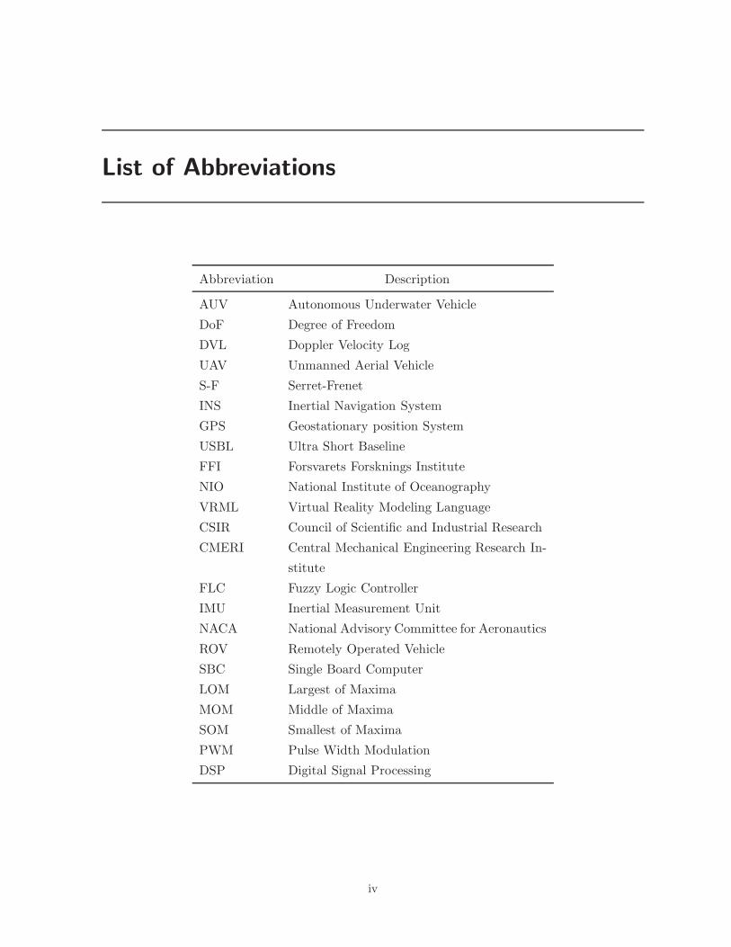
List of Abbreviations
Abbreviation Description
AUV Autonomous Underwater Vehicle
DoF Degree of Freedom
DVL Doppler Velocity Log
UAV Unmanned Aerial Vehicle
S-F Serret-Frenet
INS Inertial Navigation System
GPS Geostationary position System
USBL Ultra Short Baseline
FFI Forsvarets Forsknings Institute
NIO National Institute of Oceanography
VRML Virtual Reality Modeling Language
CSIR Council of Scientific and Industrial Research
CMERI Central Mechanical Engineering Research In-
stitute
FLC Fuzzy Logic Controller
IMU Inertial Measurement Unit
NACA National Advisory Committee for Aeronautics
ROV Remotely Operated Vehicle
SBC Single Board Computer
LOM Largest of Maxima
MOM Middle of Maxima
SOM Smallest of Maxima
PWM Pulse Width Modulation
DSP Digital Signal Processing
iv

List of Figures
1.1 Examples of Commercial AUV’s . . . . . . . . . . . . . . . . . . . . . . . . . . 2
1.2 Examples of Military application AUV’s . . . . . . . . . . . . . . . . . . . . . . 2
1.3 AUV’s used for oceanography and marine studies . . . . . . . . . . . . . . . . . 3
1.4 Structure of an AUV showing Navigation,Guidance and control schemes . . . . 3
1.5 Formation of Quadrotor [courtesy : FRAC] . . . . . . . . . . . . . . . . . . . . 5
2.1 General framework of ship path following[2] . . . . . . . . . . . . . . . . . . . . 13
2.2 Illustration of wedge formation of Leader-Follower structure . . . . . . . . . . 14
2.3 Example of virtual based formation control . . . . . . . . . . . . . . . . . . . . 15
2.4 An example of motor schemas . . . . . . . . . . . . . . . . . . . . . . . . . . . 16
3.1 Path following controller implementation . . . . . . . . . . . . . . . . . . . . . 19
3.2 Kinematics and Dynamics structure of AUV . . . . . . . . . . . . . . . . . . . 20
3.3 Control Structure for Path following . . . . . . . . . . . . . . . . . . . . . . . . 21
3.4 Representation of Serret-Frenet Frame Parameters . . . . . . . . . . . . . . . . 22
3.5 AUV Following a desired circular path . . . . . . . . . . . . . . . . . . . . . . . 29
3.6 Angular Position of AUV while traversing the circular path . . . . . . . . . . . 29
3.7 Distance error between AUV and S-F frame . . . . . . . . . . . . . . . . . . . . 30
3.8 Represents the update rate of S-F frame along the circular path . . . . . . . . 30
3.9 Variation of Surge velocity along the path . . . . . . . . . . . . . . . . . . . . . 30
3.10 Variation of Sway velocity along the path . . . . . . . . . . . . . . . . . . . . . 31
3.11 Variation of Yaw velocity along the path . . . . . . . . . . . . . . . . . . . . . 31
3.12 Thruster variation with respect to time . . . . . . . . . . . . . . . . . . . . . . 31
3.13 Rudder Variation with respect to time . . . . . . . . . . . . . . . . . . . . . . . 32
3.14 Controller gain update with respect to time . . . . . . . . . . . . . . . . . . . . 32
3.15 Comparison of path following control of an AUV along the desired path . . . . 32
3.16 Error between the path and desired path . . . . . . . . . . . . . . . . . . . . . 33
3.17 Comparison of Rudder variation of the AUV while traversing the path . . . . 33
v

LIST OF FIGURES vi
4.1 Leader-Follower Formation structure . . . . . . . . . . . . . . . . . . . . . . . . 36
4.2 Control signal flow of error space for Leader-Follower . . . . . . . . . . . . . . . 38
4.3 Development of Error space for Leader-Follower . . . . . . . . . . . . . . . . . 39
4.4 The proposed structure of formation controller for follower AUVs . . . . . . . . 40
4.5 Block diagram of the AUV with fuzzy controller . . . . . . . . . . . . . . . . . 44
4.6 Fuzzy Membership function for error along x-axis . . . . . . . . . . . . . . . . . 45
4.7 Fuzzy Membership function for error along y-axis . . . . . . . . . . . . . . . . . 45
4.8 Fuzzy membership function for surge velocity . . . . . . . . . . . . . . . . . . . 45
4.9 Fuzzy membership function of angular error . . . . . . . . . . . . . . . . . . . . 46
4.10 Fuzzy membership function for derivative of angular error . . . . . . . . . . . . 46
4.11 Fuzzy membership function for yaw velocity . . . . . . . . . . . . . . . . . . . . 46
4.12 Desired formation shape for formation control . . . . . . . . . . . . . . . . . . 49
4.13 Formation of three AUV’s maintaining a triangular shape . . . . . . . . . . . . 50
4.14 Error of the Leader AUV while traversing the desired path . . . . . . . . . . . 50
4.15 Error of follower AUV1 while following the Leader AUV . . . . . . . . . . . . . 50
4.16 Error of follower AUV2 while following the Leader AUV . . . . . . . . . . . . . 51
4.17 Surge velocity of three AUV’s while following the desired path . . . . . . . . . 51
4.18 Angular orientation of three AUV’s while following the desired path . . . . . . 51
4.19 Angular velocity of Leader AUV variation w.r.t time . . . . . . . . . . . . . . . 52
4.20 Angular velocity of Follower AUV1 variation w.r.t time . . . . . . . . . . . . . 52
4.21 Formation control using fuzzy logic controller . . . . . . . . . . . . . . . . . . . 52
4.22 Control input for surge motion using fuzzy logic controller . . . . . . . . . . . 53
4.23 Control input for yaw motion using fuzzy logic controller . . . . . . . . . . . . 53
5.1 Design of AUV model . . . . . . . . . . . . . . . . . . . . . . . . . . . . . . . . 56
5.2 VRML of AUV . . . . . . . . . . . . . . . . . . . . . . . . . . . . . . . . . . . 57
5.3 Control nodes of Leader AUV . . . . . . . . . . . . . . . . . . . . . . . . . . . 58
5.4 Graphical Visualization of Multiple AUVs . . . . . . . . . . . . . . . . . . . . . 58
5.5 AUV sensors and control planes . . . . . . . . . . . . . . . . . . . . . . . . . . 59
5.6 (a) Shape of the nose (b) Shape of the tail . . . . . . . . . . . . . . . . . . . . 60
5.7 Multiple sensor fusion for the calculation of accurate AUV states . . . . . . . 61
5.8 Circuit Diagram of DC-DC Convertor . . . . . . . . . . . . . . . . . . . . . . . 63

List of Tables
2.1 Motor Schemas of Behavior based control . . . . . . . . . . . . . . . . . . . . . 17
3.1 Symbols used for Parameters of AUV . . . . . . . . . . . . . . . . . . . . . . . 21
3.2 Infante AUV Hydrodynamic parameter [3] . . . . . . . . . . . . . . . . . . . . 28
3.3 Controller gain parameters . . . . . . . . . . . . . . . . . . . . . . . . . . . . . 28
3.4 Comparison of control algorithms . . . . . . . . . . . . . . . . . . . . . . . . . 29
4.1 Linguistic variables for input and output parameters . . . . . . . . . . . . . . . 47
4.2 Fuzzy rule base for forward motion control . . . . . . . . . . . . . . . . . . . . 47
4.3 Fuzzy rule base for angular motion control . . . . . . . . . . . . . . . . . . . . 48
4.4 Comparison of backstepping and fuzzy logic control algorithms . . . . . . . . . 49
5.1 Specifications of Single Board Computer(Roboard) . . . . . . . . . . . . . . . . 64
A.1 Position and velocities of the AUV . . . . . . . . . . . . . . . . . . . . . . . . . 72
A.2 AUV parameter definition . . . . . . . . . . . . . . . . . . . . . . . . . . . . . . 74
B.1 AUV parameters . . . . . . . . . . . . . . . . . . . . . . . . . . . . . . . . . . . 75
B.2 INFANTE AUV Hydrodynamic coefficients . . . . . . . . . . . . . . . . . . . . 75
vii

Chapter 1
Introduction
1.1 Autonomous Underwater Vehicle(AUV)
AUV refers to an autonomous robot equipped with suitable sensors and actuators which
enable it to navigate in the subsea environment. This is an autonomous robot because it
executes the assigned mission without any external human intervention.
1.2 Background
Since the last decade, the control of AUVs has attracted attention of many researchers
around the world. Control of AUV with autonomy refers to the ability of AUV to navigate
in underwater environment without any human intervention. The autonomous navigation
and control of an AUV in oceanic environment is a challenging task due to the fact that
the dynamics of AUV is very complex, time varying, nonlinear and uncertain.
AUVs find application in oil industries, defense and research organizations. Some of
these are as follows.
• AUV find applications for sea floor mapping or hydrographical surveys for the de-
velopment of subsea infrastructure or layout of pipelines for oil/gas industries [4, 5].
AUVs are also employed for the leakage detection of oil/gas from the underwater
pipelines. The usage of AUV offers great benefits in replacing human operator thus
avoiding the operating cost and risk in the extreme environment i.e. deep oceanic
environment. Some of the AUVs which are generally used for commercial purpose
are shown in Fig1.1a. It has been developed by Kongsberg Maritime and Forsvarets
Forsknings Institute (FFI) in Norway,Bluefin AUV by Bluefin Robotics.
• AUVs are also suitable for military applications and for underwater mine detection.
AUVs can also be used anti-submarine warfare and also employed in a protected area
for identification of unauthorized trespassing. In recent years, AUVs are being used
1

CHAPTER 1. INTRODUCTION 2
(a) HUGIN AUV [6] (b) Bluefin 12s AUV [7]
Figure 1.1: Examples of Commercial AUV’s
(a) AUV150 [8] (b) ALISTER100 [9]
Figure 1.2: Examples of Military application AUV’s
as means for providing warfare equipments and medicines to the affected area. Few
AUVs which are known for their application in defense and other military application
are AUV150 by CSIR-CMERI, India, TALISMAN by BAE Systems and ALISTER
100 by eca Robotics.
• AUVs play a major role for marine industries because AUVs have ability of collecting
data with minimal disturbance and with great accuracy. An AUV can also be used
for study of water quality at reservoirs/dams and also for checking the dissolved
oxygen level required for sustaining marine life. Some of the AUVs used for marine
research or environmental studies are MAYA AUV by NIO, India, MARUM AUV
by University of Bremen and SeaCat AUV by RUVSA.
In order to employ an AUV for a particular application, it is required that it should
be equipped with appropriate sensors to acquire the signals of interest for monitoring
and control. For navigation of an AUV, a fusion of sensors such as Inertial Navigational
System(INS),Geostationary Position System(GPS) are sufficient for getting the exact po-
sition and orientation. But the problem with GPS is that it does not work in underwater

CHAPTER 1. INTRODUCTION 3
(a) MAYA AUV [10, 8] (b) SeaCat AUV [11]
Figure 1.3: AUV’s used for oceanography and marine studies
Figure 1.4: Structure of an AUV showing Navigation,Guidance and control schemes
environment, So in this case, a Doppler Velocity Log(DVL) can be employed i.e. a sensor
fusion of INS/GPS/DVL is necessary. From DVL sensor, one can get accurate velocity
reading because it calculates the velocity parameter from the rate of change of seabed.
These are the primary sensors for navigation purpose, whereas sonar and camera can be
used for object detection and obstacle avoidance. There is a need of specific sensors which
are used for particular application.
1.3 AUV Structure
Most of the applications of AUV require that it should follow a desired path like pipeline or
scanning or surveillance of a desired region, these requirements lead to address a common

CHAPTER 1. INTRODUCTION 4
objective for most of the applications is navigation.
1.3.1 Navigation System
Navigation system is meant for obtaining the position and orientation of the vehicle using
INS, GPS, or other acoustic sensors. But the navigation of an AUV is difficult because the
unavailability of the sensors for giving accurate position and orientation measurements.
But with the development of DVL, Ultra Short Baseline(USBL) and many other position
measurement sensors, which can be integrated to the INS for getting accurate data. In
the navigation system, usually the sensor data get corrupted by external noises. So
signal processing has a major role in navigation system. If a state is unavailable then an
estimator can be employed to generate the missing or unmeasured state.
1.3.2 Guidance System
The guidance system deals with the desired path generation from AUVs current position
to the desired position. The major challenge in the guidance control is to generate an
optimum path for the AUV considering the obstacles between the paths. It is also nec-
essary for the AUV to follow the optimum path successfully, for this, the path feasibility
for the particular AUV should be determined. The feasible path will differ for different
AUVs depending on whether it is a fully-actuated or an underactuated system.
1.3.3 Control Structure
Control structure determines the required control forces necessary for steering the AUV
along the desired path, different objectives which can be addressed by the control structure
are trajectory tracking, path following and way point tracking. While developing a control
law, it is necessary to check the stability of the AUV states, and also the generated control
forces should reside within its maximum limit. Design of control law for a fully-actuated
system is simpler than an underactuated system but the control allocation map is to be
given major attention. In an underactuated system, it is challenging to develop a control
law together with ensuring the system stability. For both the cases it is necessary to show
the robustness and adaptation of the control structure for the external disturbances.
This focus of this thesis is to develop control algorithms for an AUV to accomplish
path following of a desired path. Besides path following, other motion control strategies
of interest are trajectory tracking and way point tracking, which are described as follows.
• Trajectory Tracking Problem: It refers to the control problem where the AUV is
required to follow a time-parameterized path. But the degree of complexity for
controller development is highly dependent on whether the system is fully-actuated
or under-actuated. It is not always reasonable to use a fully-actuated system because

CHAPTER 1. INTRODUCTION 5
Figure 1.5: Formation of Quadrotor [courtesy : FRAC]
of its cost, weight and efficiency consideration. Trajectory tracking problem can be
well defined for fully-actuated system. But it is still an active area of research for
underactuated system.
• Path Following Problem: Unlike the time parameterized point as desired for trajec-
tory tracking problem, here an entire path is considered for tracking without any
time-parameterized constraint. Path-following is well suited for underactuated sys-
tem because less number of constraints involved. For path-following problem the
path is represented with its geometrical description and the AUV needs to follow the
geometrical property of the path and eventually converges to the path .
• Way Point Tracking Problem: Unlike the trajectory tracking and path following
problems, way point tracking problem is different. Here, an AUV does not follow
a path rather a desired region is specified within a visible range. The control force
should be such that it will drive the AUV towards the region confirming the stability
criteria. In this approach, a series of way-points are placed between the AUV actual
position and desired position. The objective of this problem is control AUV so that it
reaches the desired position following the way-points. For this reason, this approach
is called way-point tracking.
1.4 Cooperative Motion
Though there are numerous advantages of using a single AUV as discussed in Section 1.2
but there are some limitations in using a single AUV. With the addition of sensors for

CHAPTER 1. INTRODUCTION 6
achieving accurate measurement of position and orientation, the cost of an AUV increases
also the payload of the AUV increases. The vehicle failure can affect the complete mission
and also if numerous data are to be collected then the operating cost for an AUV increases.
These limitations can be overcome by using multiple AUVs because for single AUV failure
other AUVs in the group can still work and also the data collection by multiple AUVs
will be faster and secured. The technological advancement in AUV research has raised
the interest among the researchers for cooperative motion. Cooperative motion of AUVs
refers to the motion of multiple AUVs for a common objective. To achieve the same,
these AUVs communicate with each other. AUVs share the data received by each AUV
and takes a common decision considering the feasibility and constraints. Due to these
features, the cooperation among the AUVs can address the problem of single AUV failure
and robustness for unknown terrain. Fig.1.5 shows the cooperative control of quadrotors.
Some of the other robots/systems employed in formations are described as follows.
• Mobile Robot: Cooperative control of a group of mobile robots is adopted in many
tasks such as in task allocation, object transportation and sensor network etc. For
cooperative control, multiple robots [12, 13] should maintain a geometrical pattern or
form a group to follow a desired path or trajectory. Some of the outdoor applications
of multiple mobile robots are security patrols, handling hazardous materials and
reconnaissance in missions etc.
• Satellite Formation: Satellite Formation is an approach to combine group of smaller
satellites to work together or replacing a larger and more expensive satellite. The
advantages of using behind the formation of satellite [14] is that it reduces the build
time, simpler designs and sensing capability is increased. The applications which
can be accomplished by formation of satellites are interferometry, environmental and
communication applications etc.
• Formation of UAV: Like mobile robots multiple UAVs also can be engaged for area
coverage and reconnaissance. A formation of multiple UAVs [15, 16] can also be used
for environmental analysis.
1.4.1 Formation Control of AUVs
Since the last decade, technological advancement has motivated the researchers towards
the formation control of multiple AUVs. Better acoustic sensors and communication
modules are developed which allow an AUV to interact with environment and with another
AUV. In formation control, a fixed geometrical shape is maintained by AUVs as the
objective is demanding. Like for mine countermeasure, all AUVs should move parallel to
each other to collect as much data as possible in a single scan. These formation structures

CHAPTER 1. INTRODUCTION 7
can be decided by a leader in a leader-follower approach or it may be a group decision in
a behavior approach. Generally the motion of multiple AUVs can be categorized under
centralized and de-centralized technique.
A centralized system requires a large amount of data on navigation to be processed by
a single unit. This unit may be a leader in a formation group or a surface ship which is
monitoring some group of AUVs. But in a centralized technique, due to huge bi-directional
data transfer, the usage of this technique is limited in real-world and also the guidance of
multiple AUVs in a difficult environment will be a tough task. Whereas in decentralized
technique there is no central processing unit and each vehicle has its own independent
controller. Here, the AUVs have the ability to sense the environment and act on their
own, which significantly reduces the cost of communication as in centralized technique.
But still the large amount of data transfer exist between the AUVs.
In this thesis, a centralized approach for formation control is considered because cen-
tralized approach provides less complexity for small number of AUVs. Many researchers
are developing and enhancing the control techniques for formation control. Some of the
generally accepted control techniques for both centralized and decentralized methods are
summed as follows
• Potential and Behavior based approach: In formation control the Behavior-based
approach and potential field approach are considered for various applications. The
basic principle behind behavior based approach is that,each AUV consists of a basic
structure called motor schemas [17]. Each motor schemas generates its corresponding
desired behavior, some of the motor schemas are collision avoidance, formation shape
and goal seeking. The control input for a AUV is generated by weighted average of
every motor schemas, thus a proper gain is adjusted using optimization technique.
Few investigations [18, 19, 20] where initial applications of behavior based control
are shown.
• Leader-Follower approach:Another approach uses leader-follower patterns in forma-
tion control. It is assumed that only local sensor based information is available for
each AUV. There are two types of feedback controllers for maintaining formations of
multiple AUVs. The leaders track predefined reference trajectories and the followers
track transformed versions of the states of their nearest neighbors according to given
schemes.
• Virtual Structure method:The concept of virtual structure was first introduced in
[21]. The virtual structure approach is usually used in spacecraft or small satellite
formation flying control [22]. Control methods are developed to force a group of
agents to behave in a rigid formation. In virtual structure approach, the controller is

CHAPTER 1. INTRODUCTION 8
derived in three steps. First, the desired dynamics of the virtual structure is defined.
Second, the desired motion of the virtual structure is translated into desired motions
for each agent. Finally, individual tracking controllers for each agent are derived for
agent tracking. In [14], the virtual structure method is combined with the leader-
following method and behavioral approach to formation control of multiple spacecraft
interferometer in deep space. In the virtual structure approach, the entire formation
is treated as a single entity. When the structure moves, it traces out the desired
trajectories for each robot in the group to track.
• Synchronization Based Control: In this method independent paths are derived from
the desired path for each autonomous vehicle. These paths act as the desired paths
but the motion of vehicle while following the respective paths should be coordinated.
In other words, it can be said that there exists a velocity and acceleration constraint
on each derived path. [23, 24, 25] are some of the works where synchronization
approach has been applied for formation of mobile robot and surface vehicles.
1.5 Motivations
The development of control law for an AUV is complex and more challenging because the
AUV is an underactuated system. Also the dynamics of AUV is very much influenced
by the external environment. With the huge application of AUV in various fields and
amongst them the path following is an basic requirement for every application.
As discussed earlier, the multiple AUVs as compared to single vehicle has better ro-
bustness towards vehicle failure and also has better data collection. For many time critical
missions such as military operation or rescue missions, the use of multiple vehicles shows
better performance as comparison to a single AUV.
1.6 Objectives of the Thesis
The objectives of the thesis are as follows.
• To develop a controller for an AUV considering thruster force and rudder plane
as control input. These control input when supplied to dynamical equation, will
steer the AUV towards the desired path. During the course of path following while
maintaining the desired surge velocity.
• To develop a controller which will drive multiple AUVs towards a desired path or
goal, while maintaining a desired shape. The controller will generate the desired
surge and yaw velocity for the followers which allows them to follow the leader AUV
maintaining the distance and orientation.
CHAPTER 1. INTRODUCTION 9
• Development of a graphical platform for visualizing the motion of an AUV and
multiple AUVs in an ocean environment.
1.7 Problem Statement
1.7.1 Path following
The objective of the path following problem is to design a control law which will steer the
AUV towards following the desired path. A path following controller for an underactuated
AUV is to be designed to track the desired path while maintaining a desired constant
velocity in the forward motion.
1.7.2 Formation control
Assuming that the information of the desired path is known to the leader AUV, and the
follower AUV should follow the leader while maintaining a particular distance in both
position and orientation. A control strategy is to be developed which enables the follower
AUVs to follow the leader and also to maintain a fixed formation structure while in
cooperative motion.
1.8 Thesis Organization
The thesis is organized as follows.
• Chapter 2 presents a literature survey on control methods of single AUV and multiple
AUVs. Studies have been made on different control strategies reported in literature
for pathfollowing. Also for achieving, successful cooperative motion, different control
strategies are reported in literature are reviewed.
• Chapter 3 presents development of a control strategy using the concept of backstep-
ping and fuzzy logic controller for path-following of an single AUV in x-y plane. The
motion along surge, sway and yaw is considered and other motion related to depth
and roll are neglected. In this chapter, the coupling of rudder angle between sway
and yaw is also taken into consideration.
• In Chapter 4, the backstepping control technique for single AUV has been extended
for obtaining formation control for multiple vehicles. In this chapter, the leader-
follower formation strategy is adopted and assuming that only leader has the infor-
mation about the path and follower follows the leader. This chapter also implements
a fuzzy logic controller for leader-follower formation control. The result of both the
controller have been presented and discussed.

CHAPTER 1. INTRODUCTION 10
• In Chapter 5, simulation on graphical interface of AUV motion control for both path
following and formation control are discussed. The graphical visualization is created
with the help of virtual-reality in SIMULINK 3D for better visualization of motion of
single AUV or multiple AUVs in an ocean environment. This chapter also discusses
about the selection of various hardware elements essential for the development and
construction of an AUV.
• Chapter 6 concludes the thesis. Scopes of extension of present work are also discussed.
• Appendix-A presents the dynamics and kinematics of the AUV. These equations
are used for the development of control algorithm for path following and formation
control.
• Appendix-B presents the AUV(INFANTE) parameters considered for implementa-
tion of the proposed control algorithms.

Chapter 2
Literature Review on Control of AUV
In the past two decades, the majority of research has been devoted in the fields of Au-
tonomous Underwater Vehicle motion control. An accurate motion control strategy is
very important, for application of AUVs in various applications such as discussed in Sec-
tion 1.2. Different motion control strategies which are generally adopted for AUV are
path following, way point tracking, trajectory and localization. These motion control
strategies are chosen based on either mission requirement or on commercial requirement.
This thesis is concerned with the development of path following control of AUV. In path
following strategy, a predefined path is assigned to the AUV and the AUV controller
generates a control law which steers and propels the AUV to move in the desired path.
But for single AUV path following control there is less requirement of sensor information.
Very often instead of using single AUV multiple AUVs are employed in a cooperative
motion control framework. This chapter reviews the reported control techniques for both
the path following control and Co-operative motion control of AUVs.
2.1 Literature Review on path-following of AUV
In order to achieve the path following control of an AUV, the error between the path
parameters and AUV position and orientation need to be reduced to zero. For this the
control inputs to the AUV are thruster force and orientation of rudder, stern plane. Also
the complete dynamics of AUV is a nonlinear 6DOF equation of motion with coupled
and nonlinear terms involving added mass, hydrodynamic damping and also external
disturbances by environment. So it is difficult to achieve accurate path following by using
linear controllers, but some investigations have considered the approximated 2nd order
linear equation of AUV for designing path following controllers. In [26] 2nd order AUV
model is approximated to 3rd order equation with the inclusion of an extra degree and its
parameters are identified by using Markov parameter. The approximated linear equation
is derived with assumption in nonlinear equation and it is suitable for specific operating
11

CHAPTER 2. LITERATURE REVIEW ON CONTROL OF AUV 12
points. There are also some investigations employing the [27] the feedback linearization
method for path following control but the linearization method or linear controllers are
suitable for particular operating point. So for highly coupled and nonlinear equations
the nonlinear controllers are suitable. Various nonlinear controllers from [28, 29, 30] can
be applied for developing path following controller considering the following nonlinear
dynamics. A number of nonlinear controllers such as backstepping controller, sliding
mode control, soft computing approach are studied and the investigations in this area are
applied are discussed below.
Fuzzy Logic controllers and sliding mode controllers have been implemented for AUV
pathfollowing [31, 32, 33]. In [31], a sliding surface is used to represent the error between
desired path and AUV position and taking this error in to consideration a fuzzy controller
has been implemented for generating the control input i.e. rudder orientation. In [32], a
sliding mode controller is designed for marine vessel but equations of motion are for 3dof
which are considered for underwater vehicle. The marine vessel which is considered in
[32] is considered to be fully actuated vehicle and in this literature the stability analysis
was made using the Lyapunov method.
Another nonlinear controller which is mostly used for the autonomous vehicles is Back-
stepping controller, a Lyapunov based controller. An initial work on path tracking of
mobile robots using the backstepping control is reported in [34]. Usually a mobile robot
can be accurately controlled with the kinematics only but in the case of AUV only kine-
matics control is not sufficient because of nonlinearity and presence of coupling terms in
the dynamics equation. In case of AUV, both the parameters of kinematics and dynamics
need to be controlled. The backstepping control has been applied to AUV considering
the complete dynamics equation in [2, 35, 36, 1] .
Referring [2], presents a path following control of an AUV by assuming a virtual ve-
hicle that follows the desired path and the error between its position and orientation has
been considered with backstepping controller. The boundedness and stability properties
of the error backstepping is also presented in [2]. A similar approach has been applied
for the path following problem of AUV [35, 36] with an exception that a Serret-Frenet
frame is considered in place of virtual vehicle. But in the development of the pathfol-
lowing controllers in [35, 36] the information for jerk parameter is required for effective
path following but in practical cases the measurement of jerk parameter is difficult to
measure. As this data is not available using any sensor so the controller heavily relies on
mathematical model, but if parameter uncertainty mathematical model is considered then
the jerk data will be an erroneous data. In [25], the S-F frame has been considered and
problem of requests jerk information has been resolved. The [1] considers the dynamics
of surface vessel which will be similar to AUV in 3DOF, but it assumes that the vessel

CHAPTER 2. LITERATURE REVIEW ON CONTROL OF AUV 13
Figure 2.1: General framework of ship path following[2]
is moving with constant forward velocity. Also the coupling term of rudder control plane
δr in the sway equation of motion is neglected. But when an AUV carries an unbalanced
payload then this term cannot be neglected because the unbalanced payload will affect
the coupling coefficient and the coefficient of the rudder control plane in sway will be
large. These shortcomings are addressed in 3 during the development of path following
controller.
2.2 Literature Review on cooperative motion of AUVs
Cooperative motion control refers to the collective behavior of multiple vehicles deployed
for the fulfillment of a common mission for example survey operation. The other forms
of cooperative motions are formation, flocking and swarming. The flocking and swarming
approach is directly inherited from the motion of ants, birds etc but in the formation
approach, multiple vehicles moves by maintaining a fixed geometrical structure. For im-
plementation of formation control strategies for mobile robots, aerial vehicles and under-
water vehicles various control strategies such as Leader-Following, Virtual structure based
and behavior based strategies have been reported. Some of the early works on formation
control focussed on mobile robots but subsequently with the development of improved
sensors and actuators these methods can be applied to aerial vehicles and underwater
vehicles.

CHAPTER 2. LITERATURE REVIEW ON CONTROL OF AUV 14
Figure 2.2: Illustration of wedge formation of Leader-Follower structure
2.2.1 Leader-Follower Control
The leader-follower strategy was first introduced by a German economist Heinrich Freiherr
von Stackelberg. For addressing the multiple criteria, multiple decision making problems
in economics.This leader-follower strategy is also known as Stackelberg strategies, later
on this strategy finds wide application in formation control of multiple vehicles. In this
strategy, the followers control laws depend upon the states of leader vehicle. The structure
of leader-follower formation is shown in Fig.2.2, where multiple vehicles follow the desired
path by maintaining a wedge like shape. During this formation, the followers have to
follow the leader and avoids the collision with the neighbor vehicles or obstacles. This
leader-follower strategy has been applied for formation of aerial, terrestrial as well as
underwater vehicles. Due to interdependence of follower vehicle on leader vehicle, the
information transfer of position and velocities is more.
In leader-follower approach, each vehicle is positioned with respect to the neighbor
vehicle to form an geometrical structure. In a leader-follower strategy there are global
leaders and also a local leader, for a particular formation group there is a single leader
but the formation may have multiple local leaders. Referring to Fig.2.2, the vehicles next
to leader vehicle will also be the local leader for the next corresponding vehicles. Among
multiple vehicles, the global leader has the information about the path trajectory. This
control structure is proposed in [37, 38, 39] for multiple mobile robots. Also transition
from one formation structure to another formation structure is also presented with the
help of graph theory. Refer [40], the leader-follower approach is also applied to underwater

CHAPTER 2. LITERATURE REVIEW ON CONTROL OF AUV 15
Figure 2.3: Example of virtual based formation control
vehicles. In this reference the dependence of follower AUV on leader states is addressed
by the addition of a Neural Network function approximation, which will provide the ap-
proximate states of leader to the follower. [41] also adopts the similar approach where the
estimator is used to estimate in the follower vehicle to estimate the velocity of the leader
vehicle. [42, 43] implements sliding mode controller and fuzzy controller for developing a
leader follower strategy among the vehicles.
2.2.2 Virtual Structure Based Control
Another approach towards formation control is Virtual Structure, where a imaginary rigid
structure is assumed and the vehicles are connected to the respective nodes. This approach
is identical to the leader-follower strategy but the difference lies in the physical presence
of the leader vehicle. In virtual structure based approach, a virtual leader is considered,
so the approach remains same for analysis. Similar to leader-follower approach the infor-
mation of position and velocities of vehicles are to be regularly transferred. Thus, usually
centralized method is adopted for implementation of virtual structure based strategy.
Referring Fig.2.3, the virtual leader follows the desired path and the location of leader
vehicle is transferred to other vehicles.
The virtual structure formation strategy adopts centralized approach but this approach
can be modified for decentralized approach by assigning a virtual leader for each follower
and a virtual leader position and orientation is calculated and communicated to each
follower. The leader follower approach where the leaders position and orientation are in-
dependent of follower vehicles results increased actuation signal. But for virtual structure
the leaders position and orientation are calculated from followers so perfect formation

CHAPTER 2. LITERATURE REVIEW ON CONTROL OF AUV 16
Figure 2.4: An example of motor schemas
structure can be guaranteed and also the less actuation signal requires to maintain the
formation. This strategy is first introduced by [21], the principle behind the the approach
is that the vehicles will move in such a way that the structure will move smoothly along
the path. [44],[45] are some of the literatures where virtual structure approach is applied
in mobile robots. An illustrative of virtual structure is represented in Fig.2.3. The ad-
vantages of virtual structure is that it is simpler to describe the coordination of multiple
vehicles. Whereas the disadvantages with the virtual structure is that it limits the po-
tential application where formation shape is time varying or when regular configuration
is required.
2.2.3 Behavior Based Formation Control
The basic idea behind the concept of behavior based formation control[30] is to assign
set of desired behaviors to each vehicles and the net control action will be the weighted
average of each behavior. Here the behavior refers to the collision avoidance, goal following
and formation keeping etc. In the literatures [20, 17, 46, 18] these behaviors are termed
as motor schemas or functions. Unlike the leader-following formation control and virtual
structure approach, less information needs to be communicated among the vehicles. But
in the later to show the global convergence of the vehicles towards the desired goal is
difficult.
From Fig.2.4, it is clear that the behavior based approach is influenced from the be-
havior of ants and bees. Refereing to [17] these kinds of flocking algorithms consist of
simple motor schemas at individual level with some level of intelligence embed into it.
One such kind of motor schemas is shown in Table.2.1. These motor schema provide the
basic structure for moving towards the target and avoiding the obstacles. Here each motor
schema provides a vector component according to the sensory input and a gain parameter
represents the importance of the particular schema. A combined behavior is generated

CHAPTER 2. LITERATURE REVIEW ON CONTROL OF AUV 17
Table 2.1: Motor Schemas Pa-rameters for Formation Naviga-tion Experiments in Simulation[17]
Parameter Value Units
Avoid-static-obstacle
Gain 1.5Sphere of influence 50 metersMinimum range 5 meters
Avoid-robot
Gain 2.0Sphere of influence 20 metersMinimum range 5 meters
Move-to-goal
Gain 0.8Noise
Gain 0.1Persistence 6 time steps
Maintain-formation
Gain 1.0Desired spacing 50 metersControlled zone radius 25 metersDead zone radius 0 meters
by summing and normalizing the result of each motor schema. In [20], these schemas
are represented as different reactive rules such as path finding, map learning, boundary
following and safe wandering. These reactive rules take the input from sensors such as
compass, sonar and fed the output to the motors for robot movement. These behavior
based approach have been applied in the field of cooperative motion of AUVs [20, 17, 46].
2.3 Chapter Summary
In this chapter, various control strategies for single AUV path following and cooperative
motion of multiple AUVs are studied and analyzed. It summarizes various controllers
implemented for successful implementation for AUV path following. For cooperative
control of multiple AUVs, various strategies has been discussed and also the literatures
on cooperative motion has been studied.
Chapter 3
Path following Control Strategy for an
Individual AUV
3.1 Introduction
Autonomous navigation and path control of an AUV possess difficult control problem
owing to the fact that AUVs are underactuated systems i.e.the control inputs are less
than degree of freedom. Navigating an AUV along a desired path is quite a difficult task
due to presence of external disturbances such as ocean disturbance and also exact AUV
parameters are unknown to the control engineers. The general navigational problems
which are usually the active area of research are path following, trajectory tracking and
waypoint tracking.
This chapter is organized as follows. In Section 3.3, we introduce the Serret-Frenet
frame and its application in path following problem. The AUV kinematics and dynamics
are discussed in Section 3.4.1 and Section 3.4.2. The error space between Serret-Frenet
frame is given in Section 3.5 for the development of control algorithm. In Section 3.6,
the control law is developed for successfully following a desired path. Finally the control
algorithm is verified by simulations which are discussed in Section 3.7.
3.2 Objective
Let the desired path, P which the AUV is to follow Fig.3.1. It is intended to design a
control law such that the AUV will follow the desired path P . Further the control of
AUV is difficult due to underactuation. A path following controller for an underactuated
AUV is to be designed such that it steers the AUV towards the desired path P while
maintaining a constant velocity in the forward motion.
As per the objective the contribution of this chapter for addressing the path following
problem are as follows.
18

CHAPTER 3. PATH FOLLOWING CONTROL STRATEGY FOR AN INDIVIDUAL AUV 19
Figure 3.1: Path following controller implementation
• Developed the path following control considering the coupling of rudder angle be-
tween sway and yaw motion.
• Surge equation of motion is considered for achieving accurate path following.
• A graphical visualization is developed using Virtual Reality Modeling Language((VRML))
for analyzing the motion of AUV.
3.3 Introduction to Serret-Frenet Frame
Serret-Frenet Frame has been independently discovered by Jean Frdric Frenet in 1847 and
Joseph Serret in 1851. Frenet presented an idea of attaching a frame at each point of the
curve in space and as the frame moves along the curve the geometric parameters such as
turn and twists can be determined. This theory of Frenet gives the six formulae of curve
in space and Joseph Alfred Serret in 1851 contributed by giving all nine formulae of curve
in space combining which makes Serret-Frenet Frame.
3.4 AUV Kinematics and Dynamics
Kinematics and dynamics of an AUV are described in Fig.3.2 where the transformation
matrix T represents the transformation of body frame to earth fixed frame. The AUV
parameter block represents the added mass and hydrodynamic coupled parameters. For
implementing the path following control in x-y domain, only 3DoF is considered i.e. surge
equation of motion is along x-direction, sway equation of motion is along y-direction and
yaw equation of motion is angular movement along z-direction. The corresponding kine-
matic equations are also considered. For derivation and explanation of AUV kinematics
and dynamics refer Appendix-A.

CHAPTER 3. PATH FOLLOWING CONTROL STRATEGY FOR AN INDIVIDUAL AUV 20
Figure 3.2: Kinematics and Dynamics structure of AUV
3.4.1 AUV Kinematics
The following are the kinematic equations for linear motion along x, y axes and rotational
motion along the z axis.
x = u cos(ψ) − v sin(ψ)
y = u sin(ψ) + v cos(ψ)
ψ = r
(3.1)
Here x, y are the linear positions whereas ψ is the angular position with reference to the
Inertial frame I. u and v are the linear velocities of AUV along x-axis and y-axis and r
is the angular velocity along z-axis.
3.4.2 AUV Dynamics
The motion of AUV along x-y plane is considered, and the components for motion contri-
bution along z-axis are neglected i.e. heave and pitch equation of motion are neglected.
The AUV considered in this work is a flat-fish type, so the roll equation of motion can be
neglected. The following equations of motion are adopted from [3].
Surge Equation of Motion:
u =m+Xvr
m−Xuvr +
Xuu
m−Xuu2 +
T
m−Xu(3.2)
Sway Equation of Motion:
v = −(
m− Yurm− Yv
)
ur +Yuv
m− Yvuv +
Yvvm− Yv
v |v| +Yuuδru
2δrm− Yv
(3.3)
Yaw Equation of Motion:
r =Nvv
Iz −Nrv |v| +
Nrr
Iz −Nrr |r| +
Nur
Iz −Nrur +
Nuv
Iz −Nruv +
Nuuδru2δr
Iz −Nr(3.4)

CHAPTER 3. PATH FOLLOWING CONTROL STRATEGY FOR AN INDIVIDUAL AUV 21
Table 3.1: Symbols used for Parameters of AUV
m Mass of the vehicleIz Inertial tensor in body frame BXu, Yv, Nr Added mass of vehicleXuu, Yvv, Nrr, Nvv Cross-flow DragXvr, Yur , Nur Added mass cross term and Fin liftYuv, Nuv Body lift force and Fin lift
Figure 3.3: Control Structure for Path following
The symbols in the above equation of motion of the AUV are listed in Table 3.1:
The AUV dynamics (3.2)-(3.4) includes the thruster force T and rudder angle δr as
control inputs. Here, it is clear that the equation of motion are coupled to each other and
highly non-linear thus, development of controller for the AUV is challenging.
3.5 Development of Error Space
This Section contributes to the development of error space of AUV with in the Serret-
Frenet frame. The error structure and notations used in this section are adapted from [1],
[47]. Referring to Fig.3.3, the controller is to be designed to reduce the error generated
in the error space. The control gains are adopted according to the error. Considering
Fig.3.4, a desired path Ω is to be followed by an AUV with body frame B attached to
its center of gravity. A Serret-Frenet (S-F) frame is attached to a point S on the path.
B is the point which can be described as (x, y)T in inertial frame I or (xe, ye)T in S-F
frame F, U is the net velocity of the AUV i.e. U =√u2 + v2, β is the angle between
net velocity and sway velocity. θsis the angle made by S-F frame with the inertial frame
I and ccis the curvature at point S.
Referring [35] velocity at point S with reference to Inertial frame is expressed as following
vS = vB +R−1
(
dBS
dt
)
+R−1(
ψd × BS)
(3.5)

CHAPTER 3. PATH FOLLOWING CONTROL STRATEGY FOR AN INDIVIDUAL AUV 22
Figure 3.4: Representation of Serret-Frenet Frame Parameters
where
R =
cos(ψd) sin(ψd) 0
− sin(ψd) cos(ψd) 0
0 0 1
,
vS = [x, y, 0]T ,
RvB = [s, 0, 0]T ,(
dBSdt
)
= [xe, ye, 0]T ,
ψd ×BS = [−ccsye, ccsxe, 0]T .
vS and vB are the velocities at point S and B expressed in inertial frame I. ψd is the angle
between a tangent at point S and x-axis of the Inertial Frame I, s is the arc length of the
desired path Ω. cc is the path curvature at point S. The position of AUV with reference
to S-F Frame is xe, ye. Rewriting (3.5) by replacing the above defined parameters is
xe
ye
0
= R
x
y
0
−
s (1 − ccye)
sccxe
0
(3.6)
For aligning the heading angle along the desired angle, the orientation error is defined
as
ψe = ψ − ψd (3.7)
and its derivative is
ψe = r − ccs (3.8)
The orientation error between total velocity U and s can be expressed as
ψ∗e = ψe + β (3.9)

CHAPTER 3. PATH FOLLOWING CONTROL STRATEGY FOR AN INDIVIDUAL AUV 23
where β = tan−1 (v/u ) and ψ∗e is described as the angular error between total velocity
U and s of S-F frame. The following equations can be derived by rewriting the (3.6) in
terms of ψ∗e .
xe = U cos (ψ∗e) − s (1 − ccye)
ye = U sin (ψ∗e) − sccxe
(3.10)
Differentiation of (3.9) gives,
ψ∗e = r + β − ccs (3.11)
3.6 Control Law Development
The error space developed in the previous section is considered here. Initially it is assumed
that ψ∗e = αψ∗
e, where αψ∗
eis the angle that describes the desired orientation for AUV to
follow the desired path. Consider a Lyapunov candidate function V1 = 12(x2
e + y2e). Taking
the derivative of the above Lyapunov equation, we have
V1 = (xexe + yeye) (3.12)
and replacing xe and ye from (3.10) in (3.12), V1 is obtained as
V1 = xe (U cos (ψ∗e) − s (1 − ccye)) + ye (U sin (ψ∗
e) − sccxe)
= xe (U cos (ψ∗e) − s (1 − ccye)) + ye (U sin (ψ∗
e) − sccxe)
= xeU cos (ψ∗e) − xes+ Uye sin (ψ∗
e)
(3.13)
It is assumed that the AUV initially moves such that it satisfies the condition i.e.
ψ∗e = αψ∗
e. Replacing ψ∗
e with αψ∗
ethen (3.13) is represented as
V1 = xeU cos(
αψ∗
e
)
− xes+ Uye sin(
αψ∗
e
)
= xe(
U cos(
αψ∗
e
)
− s)
+ Uye sin(
αψ∗
e
)
(3.14)
It is straightforward that the following choice of the update rate i.e.
s = U cos(αψ∗
e) + ksxe (3.15)
yields
V1 = −ksx2e + Uye sin(αψ∗
e) (3.16)
and as sign(ye) = −sign(αψ∗
e) always holds, thus (3.16) is always a decreasing func-
tion.The desired orientation is to be designed such that the 2nd term of V1 of (3.16) should
always be a negative term, which leads to the complete convergence of V1 to zero. The
choice of desired orientation should ensure that it is always differentiable at t = 0. Let
this function can be selected as

CHAPTER 3. PATH FOLLOWING CONTROL STRATEGY FOR AN INDIVIDUAL AUV 24
αψ∗
e= −
(
1 − e−t/τ)
θa tanh (kδye) (3.17)
where τ is the smoothing factor for αψ∗
e. Let the deviation from actual angular position
(ψ∗e) from the desired approaching angle (αψ∗
e) be defined as ψe = ψ∗
e − αψ∗
e.
The derivative of ψe while following the desired path is as follows:
˙ψe = r + β − ccs− αψ∗
e(3.18)
From (3.18), if αr is defined as the desired yaw velocity then actual yaw velocity r can be
expressed as re + αr. Rewriting (3.18) with r replaced as re + αr is
˙ψe = re + αr + β − ccs− αψ∗
e(3.19)
In terms of Backstepping method this new term αr act as a control input for (3.19). The
objective is to select the control input such that (3.19) gradually decreases to zero. Thus
a Lyapunov function V2 is considered which corresponds to the positive definite error
function for minimizing the ψeerror.
V2 =1
2ψ2e (3.20)
For minimizing the orientation error, the derivative of the Lyapunov function (3.20) should
gradually decrease to zero so that the AUV orientation gradually aligns to the desired
orientation. Taking the derivative of above Lyapunov function,
V2 =ψe˙ψe
=ψe
(
u
U2
(
Yuvm− Yv
uv +Yvv
m− Yv|v| v +
Yuuδru2δr
m− Yv
)
+ βre −v
U2
(
Xuu
m−Xuu2 +
T
m−Xu
)
+
ccs+ αψ∗
e+ βαr
)
(3.21)
and choosing the αr as following
αr = F1 + F2δr + F3T (3.22)
where
F1 =−Kψe ψe
β− u
βU2
(
Yuvm−Yv
uv + Yvvm−Yv
|v| v)
+ vβU2
(
Xuum−Xu
u2)
+ccs+αψ∗
e
β,
F2 = −uβU2
Yuuδru2
m−Yv,
F3 = vβU2m−Xu
.
by replacing αr in (3.21), the derivative of Lyapunov function V2 is expressed as following.
V2 = ψeβre −Kψeψ2e (3.23)

CHAPTER 3. PATH FOLLOWING CONTROL STRATEGY FOR AN INDIVIDUAL AUV 25
The 2nd term is a decreasing function where as the 1st term consists of βre. If re reduces to
zero then the Lyapunov function V2 gradually reduces to zero and the AUV will approach
towards the desired orientation angle. The boundedness of re parameter is considered
later in this chapter and
β =
(
1 − u2
U2
m− Yurm− Yv
− v2
U2
m+Xvr
m−Xu
)
(3.24)
which is always greater than zero and bounded.
Let ud represents the desired surge velocity. The deviation from the desired surge velocity
from the actual surge velocity can be expressed as follows
ue = u− ud (3.25)
Taking derivative of surge velocity error ue, we have
ue =m+Xvr
m−Xuvre +
m+Xvr
m−Xuvαr +
Xuu
m−Xuu2 +
T
m−Xu(3.26)
Consider a Lyapunov candidate function V3 which is a positive definite function of
surge velocity error (ue). One such Lyapunov function considered for V3 is
V3 =1
2u2e (3.27)
and taking the derivative of the Lyapunov function.
V3 = ueue (3.28)
Replacing the term ue from (3.26) into (3.28), the V3 is expressed as
V3 = uem+Xvr
m−Xuvre +
m+Xvr
m−Xuvαr +
Xuu
m−Xuu2 +
T
m−Xu(3.29)
By selecting the control input T as
T =F6
F4− F5
F4δr (3.30)
where
F4 = 1m−Xu
+ m+Xvrm−Xu
vF3,
F5 = m+Xvrm−Xu
,
F6 = −Kueue − Xuum−Xu
−(
m+Xvrm−Xu
)
vF1.
and replacing it with (3.29), then it becomes
V3 =m+Xvr
m−Xuvreue −Kueu
2e (3.31)
Where it is clear that the surge velocity error ue approaches to zero only if the 1st term
is shown as bounded or decreasing function. From (3.31) and (3.23) it is observed that

CHAPTER 3. PATH FOLLOWING CONTROL STRATEGY FOR AN INDIVIDUAL AUV 26
the following Lyapunov function will approach to zero only if yaw error re reduces to zero
or if it is a bounded function. Hence, considering the re error and taking its derivative of
re = r − αr i.e.
re =Nvv
Iz −Nrv |v| + Nrr
Iz −Nrr |r| + Nur
Iz −Nrur +
Nuv
Iz −Nruv +
Nuuδru2δr
Iz −Nr− αr (3.32)
and considering a Lyapunov function V4 = 12r2e+
12u2e+
12ψ2e for stabilization of yaw velocity
error. Taking the derivative of the defined Lyapunov function which is
V4 = rere + V2 + V3 (3.33)
and replacing V2 and V3 from (3.23) and (3.31) the expression for V4 can be expressed as
follows:
V4 = rere + ue
(
m+Xvr
m−Xuvre −Kueue
)
+ ψe(
βre −Kψeψe)
(3.34)
According to Lyapunov stability theory the derivative of the positive definite Lyapunov
function should be a negative definite. So selecting a negative definite function as
V4 = −Krer2e +
(
Nrr
Iz −Nr|r| + Nur
Iz −Nru
)
r2e −Kueu
2e −Kψeψ
2e (3.35)
In this expression the gain parameter is always considered as positive quantity and the
AUV dynamic equation parameter(
NrrIz−Nr
|r| + NurIz−Nr
u)
in the AUV dynamic equation is
always a negative quantity(refer Appendix 2). So it is clear that the error parameter of
angular velocity re reduces to zero and it is shown that (xe, ye), ψe, ue and re converges to
zero exponentially. Equating Equations (3.34) and (3.35) the following condition holds
TF7 + δrF8 − αr = F9 (3.36)
where
F7 = F3
(
NrrIz−Nr
|r| + NurIz−Nr
u)
−KreF3,
F8 =Nuuδru
2
Iz−Nr+ F2
(
NrrIz−Nr
|r| + NurIz−Nr
u)
−KreF2,
F9 = Kre (F1 − r)−βψe−(
m+Xvrm−Xu
)
uev−(
NrrIz−Nr
|r| + NurIz−Nr
u)
F1 − NuvIz−Nr
uv− NvvIz−Nr
|v| v.On solving (3.30) and (3.36), the desired value of thruster force and rudder angle can be
generated for successfully following the desired path.
Simplification of αr: Recalling the value of αr = F1 + F2δr + F3T and by replacing the
expression of Thrust from ((3.30)), then αr is expressed as:
αr = F1 +F3F6
F4
+ δr
( −uYuuδru2
βU2m− Yv
) (
1 − m+Xvr
m−Xu
v2
βU2
)
(3.37)
AsYuuδrm−Yv
<< 1 so neglecting the coefficients of δr, αr and replacing Fi : (i ∈ [1, 6])
((3.37)) can be represented as follows:
αr =−K1ψeβ
− u
βU2
(
Yuvm− Yv
uv +Yvv
m− Yv|v| v
)
− Kueuev
βU2+
ccs
β+
αψ∗
e
β(3.38)

CHAPTER 3. PATH FOLLOWING CONTROL STRATEGY FOR AN INDIVIDUAL AUV 27
Unlike in [1], αr has been obtained using the partial derivative of αr. Addition of surge
motion increases the parameters involved in αr, So it becomes difficult for finding αr
through partial derivative. A simpler procedure of applying a high pass filter with appro-
priate cut-off frequency because high pass filter can act as a differentiator. The cut-off
frequency and order of the filter is varied till the filter output is similar to the mathemat-
ical model of αr. Out of many possibilities, the following is one of the filter model which
act as differentiator for our problem. The filter chosen as 2nd order high-pass Butterworth
filter with cut-off frequency 1Hz is.
x =
[
−8.85 −39.47
1 0
]
x+
[
1
0
]
u
y =[
−8.85 −39.47]
x+ u
(3.39)
Controller Gain Update Rule:
The rate of change of gain is directly proportional to the corresponding error terms and
σi, αi : i(1...n) are considered as small positive constants. Here n is the number of
controller gains available for tuning.
Kψe = −σ1Kue + α1
(
ψ2e
)
Kue = −σ2Kue + α2
(
u2e
)
Kre = −σ3Kre + α3
(
r2e
)
Ks = −σ4Ks + α4
(
s2)
(3.40)
Boundedness of β:
Rewriting the term β from (3.24) is
β =
(
1 − u2
U2
m− Yurm− Yv
− v2
U2
m+Xvr
m−Xu
)
(3.41)
Let x1 = u2
U2
(
m−Yurm−Yv
)
and x2 = v2
U2
(
m+Xvrm+Xu
)
are the two functions then rewriting the
terms following the property A.M ≥ G.M will be as follows
u2
U2
(
m−Yurm−Yv
)
+ v2
U2
(
m+Xvrm+Xu
)
2≥
√
u2
U2
(
m− Yurm− Yv
)
v2
U2
m+Xvr
m+Xu
(3.42)
replacing the numerator term of A.M with β the above inequality can be written as
1 − β
2≥ uv
U2(3.43)
and after rearranging the inequality is represented as following
β ≤ (u− v)2
U2(3.44)
As it is a path following problem so at surge velocity(u) will not be zero at any point of
time and from the inequality it is clear that β will never be zero and is bounded quantity.

CHAPTER 3. PATH FOLLOWING CONTROL STRATEGY FOR AN INDIVIDUAL AUV 28
Table 3.2: Infante AUV Hydrodynamic parameter [3]
m=2234.5kg Iz=2000 N.m.s2
Xu=-141.9 kg Xuu=-35.4 kg/mYv=-1715.4 kg Yvv=-667.5 kg/mNr=-1349 kg.m2/rad Nrr=-310Nvv=433.8 kg Xvr=1715.4 kg/radYur=103.4 kg/rad Nur=-1427 kg.m/radYuv=-346.76 kg/m Nuv=-686.08 kg
Table 3.3: Controller gain parameters
σ1=0.01 α1=0.02σ2=0.04 α2=0.08σ3=0.01 α3=0.08σ4=0.04 α4=0.4
3.7 Results and Discussions
Simulations are performed using MATLAB for verifying the performance of backstepping
control law for steering the AUV to desired Serret-Frenet frame path. For the above
simulations, AUV parameters used as given in Table 3.2[3]. The parameters for updating
the controller gains are given in Table 3.3. The initial conditions for simulation are taken
as [s, x, y, ψ, u, v, r, k1, k2, k3] = [0, 0, 0, 0, 0.5, 0, 0, 0, 0, 0]. Fig.3.5 and Fig.3.6 show the the
AUV position and orientation while following the desired circular path. The error between
AUV position and Serret-Frenet frame is plotted in Fig.3.7. As the initial distance is more
between S-F frame and AUV, so the update rate shown in Fig.3.8 initially increases and
then maintains a uniform update rate. While following the circular path, the variation of
surge and sway velocities are shown in Fig.3.9 and Fig.3.10. The yaw velocity is shown
in Fig.3.11. For maintaining the desired velocity i.e. ud = 1 and traversing the path, the
controller of AUV generates the desired thruster force and rudder angle. Fig.3.12 and
Fig.3.13 show the thruster force and rudder angle required while following the circular
path. According to the error in position and orientation the controller gains are adjusted
and is shown in Fig.3.14. The effectiveness of the derived controller has been compared
with controller developed in [1]. Fig.3.16 compares the effectiveness of the derived con-
troller and [1]. From the figure it is clear that the developed control algorithm results
better performance because the surge motion dynamics is introduced and the adaptive
control gains are implemented. Initially the error between the origin of the desired path
and AUV frame is more and gradually as AUV approaches to the path the error should
be decreasing, this result is shown in Fig.3.16. Fig.5(a) also demonstrates the comparison
between the generated rudder input from the respective control algorithms. For the same
path the control actuation differs, the controller actuation with lesser variation shows less
power consumption. It is clear that the developed control algorithm performs better than

CHAPTER 3. PATH FOLLOWING CONTROL STRATEGY FOR AN INDIVIDUAL AUV 29
−100 −50 0 50 100
−100
−50
0
50
100
X-Position [m]Y-P
osition[m
]
Desired PathActual Path
Figure 3.5: AUV Following a desired circular path
0 100 200 300 400 500 600−8
−7
−6
−5
−4
−3
−2
−1
0
Time [s]
AngularPosition[rad]
Figure 3.6: Angular Position of AUV while traversing the circular path
Table 3.4: Comparison of control algorithms
Comparison Reaching Time(sec) Rudder Variation(rad)Ghommam et.al ≈ 1500 min = −0.51,max = 0.99Developed Algorithm ≈ 600 min = −0.06,max = 0.66
the control algorithm presented in [1]. Table 3.4 shows the comparison of two control
algorithms on the basis of reaching to the path and variation of rudder input.
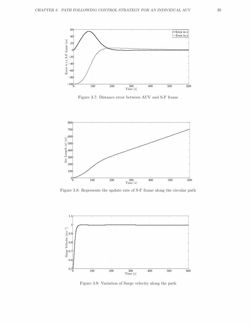
CHAPTER 3. PATH FOLLOWING CONTROL STRATEGY FOR AN INDIVIDUAL AUV 30
0 100 200 300 400 500 600−100
−80
−60
−40
−20
0
20
40
60
Time [s]
Errorw.r.tS-F
frame[m
]
Error in xError in y
Figure 3.7: Distance error between AUV and S-F frame
0 100 200 300 400 500 6000
100
200
300
400
500
600
700
800
Time [s]
Arc
Len
gth
(s)[m
]
Figure 3.8: Represents the update rate of S-F frame along the circular path
0 100 200 300 400 500 6000.5
0.6
0.7
0.8
0.9
1
1.1
Time [s]
SurgeVelocity
[ms−1]
Figure 3.9: Variation of Surge velocity along the path

CHAPTER 3. PATH FOLLOWING CONTROL STRATEGY FOR AN INDIVIDUAL AUV 31
0 100 200 300 400 500 6000
0.02
0.04
0.06
0.08
0.1
Time [s]
Sway
Velocity
(v)[m
s−1]
Figure 3.10: Variation of Sway velocity along the path
0 100 200 300 400 500 600−0.025
−0.02
−0.015
−0.01
−0.005
0
Time [s]
Angularvelocity
(r)[rads−1]
Figure 3.11: Variation of Yaw velocity along the path
0 100 200 300 400 500 6000
20
40
60
80
100
120
Time [s]
Thruster
Force[N
]
Figure 3.12: Thruster variation with respect to time

CHAPTER 3. PATH FOLLOWING CONTROL STRATEGY FOR AN INDIVIDUAL AUV 32
0 100 200 300 400 500 600−0.2
0
0.2
0.4
0.6
0.8
Time [s]
Rudder
Variation[rad]
Figure 3.13: Rudder Variation with respect to time
0 100 200 300 400 500 6000
0.05
0.1
0.15
0.2
Time
Con
trol
ler
Gai
ns
K1
K2
K3
K4
Figure 3.14: Controller gain update with respect to time
0 500 1000 1500−200
−150
−100
−50
0
50
100
150
200
X-position [m]
Y-position[m
]
Desired PathPath following using Ghomam et.alPath following using derived algorithm
Figure 3.15: Comparison of path following control of an AUV along the desired path

CHAPTER 3. PATH FOLLOWING CONTROL STRATEGY FOR AN INDIVIDUAL AUV 33
0 200 400 600 800 1000 1200 1400 1600 1800−100
−80
−60
−40
−20
0
20
40
Time [sec]
Errorw.r.tSerret-Frenet
Frame[m
]
Error in XError in Y
Figure 3.16: Error between the path and desired path
0 200 400 600 800 1000 1200 1400 1600 1800
−0.5
0
0.5
1
Time [sec]
Rudder
Variation[rad]
Ghommam et.al EBC Proposed
Figure 3.17: Comparison of Rudder variation of the AUV while traversing the path

CHAPTER 3. PATH FOLLOWING CONTROL STRATEGY FOR AN INDIVIDUAL AUV 34
3.8 Chapter Summary
In this chapter, a Lyapunov based backstepping approach to design an adaptive path
following control of an AUV is developed considering both kinematics and dynamics. Here,
Serret-Frenet frame approach for path following is chosen and a Lyapunov positive definite
function is chosen for minimizing the corresponding error in position and orientation and
from there using backstepping method a control law is derived which drives the AUV to
the desired S-F frame.

Chapter 4
Formation Control of Multiple Autonomous
Vehicles
4.1 Introduction
Formation control of multiple AUVs is an challenging research topic among many re-
searchers. Recently the research interests are increasingly employing towards multiple
AUVs because robustness is achieved in the mission to handle situations such as single
vehicle failure and also use of multiple vehicle reduces the amount of work by single ve-
hicle. For many applications such as surveillance, mine counter measure instead of single
AUV, a group of AUVs are deployed to follow a desired path while maintaining an as-
signed geometrical shape. In brief, the formation control is referred as controlling the
relative position and orientation of a number of AUVs in a group while the group as a
whole follows a desired path.
This chapter is organized as follows. The kinematics and dynamics of leader and
follower AUV are discussed in Section 4.3. This chapter is composed of two formation
controller, Section 4.4 develops the formation control using backstepping control strat-
egy and Section 4.5.1 using fuzzy logic controller. The error space is developed between
Leader and Follower AUV in Section 4.4.1 for the development of formation control law.
In Section 4.4.2, a formation control law for Follower AUV is developed for successfully
following the Leader AUV, whereas the Leader AUV follows the desired path as discussed
in the previous chapter 3. Finally the effectiveness of the above developed control algo-
rithm is verified by pursuing simulation studies and are presented in Section 4.6. This
chapter concludes with summary in Section 4.7.
35

CHAPTER 4. FORMATION CONTROL OF MULTIPLE AUTONOMOUS VEHICLES 36
Figure 4.1: Leader-Follower Formation structure
4.2 Problem Statement
Let the desired path is known to the leader AUV, and the follower AUV should maintain
a particular distance in both position and orientation. The control design for leader AUV
is implemented as discussed in the previous chapter 3. A general approach for leader
follower formation is shown in Fig.4.1, where follower should follow the leader along with
maintaining a particular distance from the leader and also with a desired orientation from
the leader. During the development of control law, we assumed that the cooperative
motion is restricted in x-y plane.
4.3 Kinematics and Dynamics of Leader and follower AUVs
For formation control of multiple AUVs the kinematics and dynamics of the leader and
follower AUV’s are assumed to be same. But for the follower AUV, the rudder angle
coupling between sway motion and yaw motion is not considered for simplicity. Thus, the
kinematics and dynamics of the leader and follower AUVs are described as follows.
4.3.1 Leader AUV
The following are the kinematic equations for leader AUV along x, y axes and rotational
motion along the z axis.
xL = uL cos(ψL) − vL sin(ψL)
yL = uL sin(ψL) + vL cos(ψL)
ψL = rL
(4.1)

CHAPTER 4. FORMATION CONTROL OF MULTIPLE AUTONOMOUS VEHICLES 37
where, xL, yL are the leader AUV position and ψL is the AUV angular position with
reference to the Inertial frame I. uL, vL are the leader velocities along the surge and sway
motion and rL is the angular motion along yaw direction.
Assuming that the dynamics of AUV considered in previous chapter 3 is the same for the
leader AUV. The following are the dynamics of the leader AUV,
The equation of motion along surge direction can be expressed as
uL =m+Xvr
m−Xu
vLrL +Xuu
m−Xu
uL2 +
TLm−Xu
(4.2)
The equation of motion along sway direction can be expressed as
vL = −(
m− Yurm− Yv
)
uLrL +Yuv
m− YvuLvL +
Yvvm− Yv
vL |vL| +YuuδruL
2δrm− Yv
(4.3)
The equation of motion along yaw direction is given by
rL =Nvv
Iz −Nr
vL |vL| +Nrr
Iz −Nr
rL |rL| +Nur
Iz −Nr
uLrL +Nuv
Iz −Nr
uLvL +NuuδruL
2δrLIz −Nr
(4.4)
The hydrodynamic parameters of the AUV are defined in Table 3.1. TL and δrL are the
thruster force and rudder orientation for the leader AUV. The control laws are developed
as described in Section 3.6.
4.3.2 Follower AUV
This Section describes the kinematics and dynamics for the follower AUVs. As we assumed
that the kinematics and dynamics for leader and follower AUV are the same, the kinematic
equations of the followerAUVs can be represented as
xF = uF cos(ψF ) − vF sin(ψF )
yF = uF sin(ψF ) + vF cos(ψF )
ψF = rF
(4.5)
where to xF , yF are the positions and ψF is the angular position with reference to the
Inertial frame I for the follower vehicles. uF , vF are the follower velocity along surge and
sway motion and rF is the angular motion along the yaw direction.
The dynamics considered for follower AUV is the same with that of the leader AUV but
the coupling of rudder angle between sway and yaw motion is not considered in follower
AUV for simplicity. So the dynamics of the follower AUV can be expressed as,
uF =m+Xvr
m−XuvF rF +
Xuu
m−XuuF
2 +TF
m−Xu(4.6)

CHAPTER 4. FORMATION CONTROL OF MULTIPLE AUTONOMOUS VEHICLES 38
Figure 4.2: Control signal flow of error space for Leader-Follower
The equation of motion along sway direction is given by
vF = −(
m− Yurm− Yv
)
uF rF +Yuv
m− YvuF vF +
Yvvm− Yv
vF |vF | (4.7)
The equation of motion along yaw direction is given by
rF =Nvv
Iz −Nr
vF |vF | +Nrr
Iz −Nr
rF |rF | +Nur
Iz −Nr
uF rF +Nuv
Iz −Nr
uFvF +NuuδruF
2δrLIz −Nr
(4.8)
where TF and δrF are the thruster force and rudder orientation for the follower AUVs.
These control inputs are obtained by designing the controller such that it enables the
follower AUV to move in a desired formation structure.
4.4 Backstepping Strategy for Formation Control
4.4.1 Error Space Development
In this Section the error space between the leader AUV and the follower AUVs for the
desired formation structure is developed considering the states of the leader AUV and
the desired position and orientations as shown in Fig.4.2. For leader-follower formation
it is required that the follower should maintain a desired distance at a particular angle.
Hence, referring to Fig.4.3, a virtual frame is defined at the desired location of xFD and
yFD which satisfies the desired distance d and desired angle θδ from the leader AUV.
The orientation of the virtual frame is considered as the same as that of leader AUV
i.e. ψL. Let the initial position of follower AUV be xF and yF with an orientation of
ψL. Then the error between the follower AUV and desired frame can be expressed with
reference to the follower AUV as xEF and yEF .
The desired location for virtual frame is considered at a distance d and orientation θδ

CHAPTER 4. FORMATION CONTROL OF MULTIPLE AUTONOMOUS VEHICLES 39
Figure 4.3: Development of Error space for Leader-Follower
from the leader AUV. Then the position of desired frame can be expressed as
xFd = xL + d cos(θδ − ψL)
yFd = yL − d sin(θδ − ψL)(4.9)
The difference between the desired frame and follower frame is considered as the error
space. This error space enables the follower AUV to approach to the desired position and
the error between follower frame and the desired frame is given by[
xEF
yEF
]
=
[
cosψF sinψF
− sinψF cosψF
][
xFd − xF
yFd − yF
]
(4.10)
Taking the derivative of the above error equation and expressing in an expanded form one
obtains
xEF = (xFd − xF ) cos (ψF ) − (xFd − xF ) sin (ψF ) rF + (yFd − yF ) sin (ψF )
+ (yFd − yF ) cos (ψF ) rF (4.11)
yEF = − (xFd − xF ) sin (ψF ) − (xFd − xF ) cos (ψF ) rF + (yFd − yF ) cos (ψF )
− (yFd − yF ) sin (ψF ) rF (4.12)
By replacing the xF and yF from the kinematics equation of follower AUV described in
(4.5), then the equation.4.11 can be expressed as
xEF = uL cos (ψL − ψF ) − vL sin (ψL − ψF ) + rLd sin (θδ − ψL + ψF ) + rF yEF − uF
yEF = uL sin (ψL − ψF ) + vL cos (ψL − ψF ) + rLd cos (θδ − ψL + ψF ) − rFxEF − vF
(4.13)

CHAPTER 4. FORMATION CONTROL OF MULTIPLE AUTONOMOUS VEHICLES 40
Figure 4.4: The proposed structure of formation controller for follower AUVs
and by substituting uL = UL cosβL and vL = UL sin βL in the above equation then can
be expressed in a more compact form. Hence the final expression for error space between
leader and follower AUV can be represented as follows
xEF =UL cos (ψ∗EF ) + rLd sin (θδ − ψL + ψF ) + rFyEF − uF
yEF =UL sin (ψ∗EF ) + rLd cos (θδ − ψL + ψF ) − rFxEF − vF
(4.14)
where ψ∗EF = βL + ψL − ψF , the above error equation represents the error space with
reference to x and y axis and ψ∗EF represents the orientation difference between leader
AUV and follower AUV.
4.4.2 Control Law Development
For developing the control law for follower AUV, the Lyapunov functions are defined which
are functions of error space developed in the Section 4.4.1. By solving these Lyapunov
functions and considering the positive constant gains, it can be shown that the close loop
is stable.
Initially it is assumed that ψ∗EF = αψ∗
EF, where αψ∗
EFis the angle that describes the
desired orientation for follower AUV to follow the leader AUV.A Lyapunov function V1F
is considered for minimizing the error between virtual frame and actual body frame of
follower AUV. Let the Lyapunov function is defined as
V1F =1
2
(
x2EF + y2
EF
)
(4.15)
In order for the closed loop system to be stable the derivative of the Lyapunov function
should always be negative. Hence, taking the derivative of the V1F leads to
V1F = xEF xEF + yEF yEF (4.16)
and replacing xEF and yEF in (4.17) from (4.14), the expression of V1F can be represented
as
V1F = U cos (ψL − ψF + β)xEF + rLd sin (θδ − ψL − ψF )xEF − uFxEF
+ U sin (ψL − ψF + β) yEF + rLd cos (θδ − ψL − ψF ) yEF − vF yEF (4.17)

CHAPTER 4. FORMATION CONTROL OF MULTIPLE AUTONOMOUS VEHICLES 41
Assuming that ψL − ψF + β = αF , where αF is the desired orientation of follower AUV
and rewriting the above equation by taking xEF and yEF as common variables as follows
V1F = (U cos (αF ) + rLd sin (θδ − ψL − ψF ) − uF )xEF
+ (U sin (αF ) + rLd cos (θδ − ψL − ψF ) − vF ) yEF (4.18)
From (4.18) if uF is selected as follows
uF = KxEF tanh (xEF ) + UL cos (ψL − ψF + βL) + rLd sin (θδ − ψL − ψF ) (4.19)
then (4.18) can be represented as
V1F = −xEFKxEF tanh (xEF ) + yEFU sin (αF ) + yEF (rLd cos (θδ − ψL − ψF ) − vF )
(4.20)
The term yEFU sin (αF ) is always be negative if the desired orientation αF is chosen as
αF = −θa tanh (KδF yEF ) (4.21)
Thus, in chapter 3 the stability of the leader motion is shown as stable, so it can be
concluded that rLd cos (θδ − ψL − ψF ) < ε as rL has a definite value and ε has a definite
value. Later of the stability proof it is shown that vF is also bounded. As yEF has a finite
range then the total Lyapunov function is always a bounded function.
Let the deviation of actual angular position from the the desired angular is defined by
ψEF = ψ∗EF − αψ∗
EF. Then its derivative can be expressed as,
˙ψEF =ψL − ψF +uLvL − vLuL
UL− αF
=rL − rF +uLvL − vLuL
UL− αF
(4.22)
Introducing the term αrF which represents the desired angular velocity for the follower
AUV. Then defining a Lyapunov candidate function V2F , which is a function of ψEF .
Defining a Lyapunov function V2F which is a positive definite function of ψeF . Let the
defined Lyapunov function is given as follows,
V2F =1
2ψ2EF (4.23)
then differentiating it with respect to time and replacing ˙ψEF from (4.22), the V2F can
be represented as
V2F =ψEF˙ψEF
=ψEF
(
rL − rF +uLvL − vLuL
UL− αF
) (4.24)

CHAPTER 4. FORMATION CONTROL OF MULTIPLE AUTONOMOUS VEHICLES 42
in the above equation rF = reF + αrF and αrF is the desired yaw velocity. Applying
backstepping approach and choosing αrF as the control input then by assigning
αrF = rL +uLvL − vLuL
UL− αF +KψEF ψEF (4.25)
the (4.24) can be expressed as
V2F = −rEF ψEF −KψEF ψ2EF (4.26)
From the expression of V2F , it is clear that if rEF reduces to zero, then the error function
V2F reduces to zero. Referring to (4.19), the desired surge velocity is developed and it is
required that the actual surge velocity should approach to the desired velocity. To avoid
confusion in parameter notations, the uF of (4.19) is replaced as uFd. The uFd for the
follower AUV is represented as following
uFd = KxEF tanh (xEF ) + UL cos (ψL − ψF + βL) + rLd sin (θδ − ψL − ψF ) (4.27)
The deviation of actual surge velocity from desired surge velocity is represented as,
ueF = uF − uFd (4.28)
and taking its derivative and replacing rF with reF + αrF results the following equation.
ueF =
(
m+Xvr
m− Xu
)
vF reF +
(
m+Xvr
m− Xu
)
vFαrF +
(
Xuu
m− Xu
uF2
)
+
(
TuFm− Xu
)
− uFD
(4.29)
A Lyapunov function V3F is considered for reducing the error of surge velocity, the Lya-
punov function is defined as
V3F =1
2ueF
2 (4.30)
where ueF = uF − uFd is the difference between actual surge velocity and desired surge
velocity. Taking the derivative of the Lyapunov function V3F and replacing it with required
ueF from (4.29), then the V3F is given by
V3F = ueF
(
m+Xvr
m− Xu
)
vF reF+
(
m+Xvr
m− Xu
)
vFαrF+
(
Xuu
m− Xu
uF2
)
+
(
TuFm− Xu
)
−uFD
(4.31)
As the expression includes thruster force as control input. So if this control input TuF is
selected as follows
TuF = (−KuEFuEF + uFD)(
m− Xu
)
−XuuuF2 − (m+Xvr) vFαrF (4.32)
then the derivative of the Lyapunov function V3F can be represented as following,
V3F =
(
m+Xvr
m−Xu
)
vF reFueF −KuEFuEF2 (4.33)

CHAPTER 4. FORMATION CONTROL OF MULTIPLE AUTONOMOUS VEHICLES 43
It is clear from (4.33) that if vF rEF is proved to be a bounded or decreasing function
then the actual surge velocity of follower AUV will approach to the desired surge velocity.
Gain KuF is considered as a positive gain. Analyzing (4.26) and (4.33), it is clear that if
the error in yaw angular velocity decreases then the follower AUV is globally stable and
approaches to the virtual frame exponentially.
Recalling the expression for yaw error velocity rEF = rF − αrF , taking its derivative
and with replacing with rF from (4.8), rEF can be expressed as
rEF =Nvv
Iz −NrvF |vF |+
Nrr
Iz −NrrF |rF |+
Nur
Iz −NruF rF+
Nuv
Iz −NruFvF+
NuuδruF2δrL
Iz −Nr−αrF
(4.34)
Defining a Lyapunov function V4F , which is a positive definite function of the yaw velocity
error rEF as follows
V4F =1
2reF
2 + V2F + V3F (4.35)
Taking the derivative of the Lyapunov function and replacing V2F and V3F from (4.26)
and (4.33) is represented as follows
V4F = reF reF − rEF ψEF −KψEF ψ2EF +
(
m+Xvr
m−Xu
)
vF reFueF −KuEFuEF2 (4.36)
From the above Lyapunov function replacing reF from (4.34) and considering the rudder
orientation as
δrF =
(
Nuuδr
Iz −NruF
2
)−1 (
−KreF reF − m+Xvr
m−XuvFueF + ψeF − Nuv
Iz −NruFvF
− Nvv
Iz −Nr
|vF | vF + αrF −(
Nrr
Iz −Nr
|rF | +Nur
Iz −Nr
uF
)
αrF
)(4.37)
then the derivative of the Lyapunov function V4F can be considered as follows,
V4F = −KψeF ψ2eF −KueFueF
2 −KreF reF2 +
(
Nrr
Iz −Nr|rF | +
Nur
Iz −NruF
)
reF (4.38)
In the above expression of V4F , KreF are positive gains and referring to the hydrodynamic
parameters of AUV it is clear that(
NrrIz−Nr
|rF | + NurIz−Nr
uF
)
is always a negative quantity.
So it is proved that by choosing the control law given in (4.32) and (4.37) for thruster
force and rudder angle respectively.An optimization approach can be implemented [48]
for adjusting the gain of the followers for better formation control.
4.5 Fuzzy Controller for Formation Control
Since the dynamics of an AUV is uncertain and the formation control of multiple AUVs
involve several uncertainties. Further a fuzzy logic controller is employed in this section

CHAPTER 4. FORMATION CONTROL OF MULTIPLE AUTONOMOUS VEHICLES 44
Figure 4.5: Block diagram of the AUV with fuzzy controller
for achieving formation control. The overview structure of the closed loop of the plant
and controller is shown in Fig.4.5. As shown in the figure the error block calculates the
error and error derivative between the current state of the AUV and desired signal. Fuzzy
logic controller accepts these errors and generates the suitable control input which enables
the AUV to successfully track the desired path. The Fuzzy Logic Controller is derived
considering the AUV kinematics and it is assumed that there exists another controller
which stabilizes the inner loop.
4.5.1 Design of Fuzzy Logic Controller
For developing the fuzzy logic controller(FLC) the error inputs considered are xEF and
yEF , these errors are the distance between the follower AUV and the desired virtual frame
as shown in Fig.4.3. Considering the plant as AUV kinematics as in (4.5) the fuzzy logic
controller is designed to generate the suitable control input uF and rF which will drive
the follower to the virtual frame. From the Fig.4.3, xEF and yEF is used to design the
FLC for the uF control input. FLC for rF control input is designed using the angular
error θE and θE , where θE can be defined as
θE = −θA tanh (KyEF ) (4.39)
Linguistic Variables
There are six i/o parameter used to develop the FLC, the linguistic used to describe the
states of these parameters are defined in Table.4.1.
Membership Function
For defining the fuzzy variables the trapezoidal membership functions are chosen. For
input and output variables the states are represented as linguistic variables and each
variable is associated with trapezoidal membership function.

CHAPTER 4. FORMATION CONTROL OF MULTIPLE AUTONOMOUS VEHICLES 45
−50 −40 −30 −20 −10 0 10 20 30 40 50
0
0.2
0.4
0.6
0.8
1
xEF
Deg
ree
of m
embe
rshi
p
VN N SN Z SP P VP
Figure 4.6: Fuzzy Membership function for error along x-axis
−50 −40 −30 −20 −10 0 10 20 30 40 50
0
0.2
0.4
0.6
0.8
1
yEF
Deg
ree
of m
embe
rshi
p
VN N SN Z SP P VP
Figure 4.7: Fuzzy Membership function for error along y-axis
0 0.2 0.4 0.6 0.8 1 1.2 1.4 1.6 1.8 2
0
0.2
0.4
0.6
0.8
1
uF
Deg
ree
of m
embe
rshi
p
VMin Min SMin N SMax Max VMax
Figure 4.8: Fuzzy membership function for surge velocity

CHAPTER 4. FORMATION CONTROL OF MULTIPLE AUTONOMOUS VEHICLES 46
−3 −2 −1 0 1 2 3
0
0.2
0.4
0.6
0.8
1
θE
Deg
ree
of m
embe
rshi
p
VN N SN Z SP P VP
Figure 4.9: Fuzzy membership function of angular error
−3 −2 −1 0 1 2 3
0
0.2
0.4
0.6
0.8
1
θE
Deg
ree
of m
embe
rshi
p
VN N SN Z SP P VP
Figure 4.10: Fuzzy membership function for derivative of angular error
−0.2 −0.15 −0.1 −0.05 0 0.05 0.1 0.15 0.2
0
0.2
0.4
0.6
0.8
1
rF
Deg
ree
of m
embe
rshi
p
VN N SN Z SP P VP
Figure 4.11: Fuzzy membership function for yaw velocity

CHAPTER 4. FORMATION CONTROL OF MULTIPLE AUTONOMOUS VEHICLES 47
VN Very NegativeN NegativeNS Negative SmallZ ZeroPS Positive SmallP PositiveVP Very PositiveVMIN Very MinimumMIN MinimumSMIN Small MinimumN NormalSMAX Small MaximumMAX MaximumVMAX Very Maximum
Table 4.1: Linguistic variables for input and output parameters
Table 4.2: Fuzzy rule base for forward motion control
For developing the controller for follower AUVs two rule base is designed as it has
two control inputs. These rule base are the knowledge base and these are implemented
using IF - THEN rules. A proper rule base is to be designed which will force the follower
AUV to steer towards the desired frame. The rule base table explains the relationship
between input and output fuzzy variables defined as membership function. Table.4.2 is
designed for the control of surge motion of the AUV. The rule base can be designed by
analyzing the behavior of the AUV under control. For designing the rule base for forward
motion it is considered that if xEF is positive which means follower is behind the leader
then the surge velocity(uF ) should increase. Similarly if xEF is negative i.e. follower
is ahead of leader then the desired surge velocity (uF ) should be a fixed nominal value.
The yEF input controls the magnitude of the surge velocity of the AUV. If yEF is more
than the magnitude of the surge velocity will decrease irrespective of xEF . Table.4.3 is
designed for the control of angular motion of the AUV i.e. yaw motion. Initially the

CHAPTER 4. FORMATION CONTROL OF MULTIPLE AUTONOMOUS VEHICLES 48
Table 4.3: Fuzzy rule base for angular motion control
angular error(θE) and derivative of the angular error(θE) are derived using xEF and yEF
as in (4.39). Considering the error and change of error a fuzzy rule base is designed which
imitates the properties of PD control. For example if θE is Positive Small(SP) and θE is
Negative Small(NS) then control output rF will be Zero(Z).
Defuzzification
After implementing the fuzzy inference system the output will be a fuzzy and it should
be transformed to crisp value for supplying to the plant. The method of conversion of
fuzzy variable to crisp variable is called defuzzification. There are different defuzzification
techniques are available such as centroid, bisector, Middle of Maximum(MOM), Smallest
of Maximum(SOM) and Largest of Maximum(LOM). Out of this for our system the
centroid method is adopted because of its simplicity. The following is the expression for
centroid method technique,
xt =
∫
µi (x) xdx∫
µi (x) dx(4.40)
where xt is the net output of the defuzzifier, x is the fuzzy output and µi represents the
aggregate membership function.
4.6 Results and Discussions
The formation control law derived in the Section 4.4.2 was simulated using MATLAB and
the control law for the leader AUV control law which was derived for the single AUV in
the chapter 3. The desired shape for the formation control is chosen as a triangular shape
as shown in Fig.4.12. It is assumed that the dynamics of the follower AUVs is same as
that of the leader AUV.

CHAPTER 4. FORMATION CONTROL OF MULTIPLE AUTONOMOUS VEHICLES 49
Figure 4.12: Desired formation shape for formation control
Table 4.4: Comparison of backstepping and fuzzy logic control algorithms
Comparison Surge velocity(uf) Yaw velocity(rf ) Velocity profileBackstepping Controller uf ≤ 1.1 −0.15 ≤ rf ≤ 0.2 smoothFuzzy Logic Controller uf ≤ 1.3 −0.032 ≤ rf ≤ 0.068 switching
Fig.4.13 shows the effectiveness of the backstepping controller for the formation of three
AUVs in a triangular shape. While traversing the desired path the error corresponding to
the leader AUV position and the desired path is shown in Fig.4.14. The error for follower
AUVs to maintain the desired triangular shape are shown in Fig.4.15 and Fig.4.16.The
desired surge velocity for the leader AUV is provided as 1m/sec as shown in Fig.4.17 for
traversing the circular path. Intuitively it can be said the velocity of follower AUV which
is inside the circular path should have lower surge velocity than the leader AUV. Whereas
the follower AUV which is at the outer of the circular path should have higher velocity
than the leader AUV. This is observed in Fig.4.17. The yaw orientation of the three AUV’s
are shown in Fig.4.18. Whereas, Fig.4.19 represents the angular yaw velocity of the leader
AUV and Fig.4.20 are the angular yaw velocities for the respective follower AUVs. The
results of the fuzzy logic controller which is derived in Section 4.5.1 are presented here,
Fig.4.21 shows the formation control of the leader-follower. The control inputs which
are required to drive the follower AUV kinematics towards the leader AUV are surge
velocity(uf ) and yaw velocity(rf ). These generated control inputs are represented in
Fig.4.22 and Fig.4.23 respectively. Table 4.4 shows the comparison between backstepping
and fuzzy logic controller.

CHAPTER 4. FORMATION CONTROL OF MULTIPLE AUTONOMOUS VEHICLES 50
−250 −200 −150 −100 −50 0 50 100 150 200 250−250
−200
−150
−100
−50
0
50
100
150
200
250
X-axis [m]
Y-axis
[m]
Desired PathLeader First FollowerSecond Follower
Figure 4.13: Formation of three AUV’s maintaining a triangular shape
0 200 400 600 800 1000 1200−200
−150
−100
−50
0
50
100
Time [s]
Error[m
]
Error in XError in Y
Figure 4.14: Error of the Leader AUV while traversing the desired path
0 100 200 300 400 500 600 700 800−10
−5
0
5
10
15
20
25
30
Time [s]
Error[m
]
Error in xError in Y
Figure 4.15: Error of follower AUV1 while following the Leader AUV
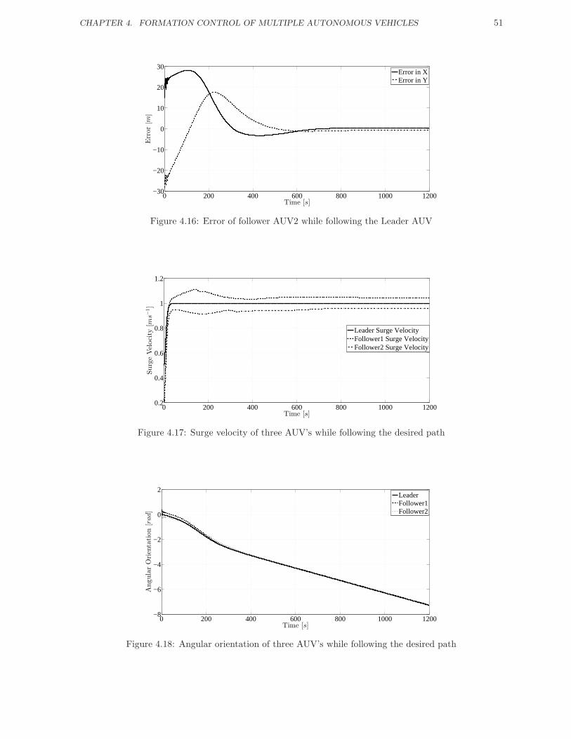
CHAPTER 4. FORMATION CONTROL OF MULTIPLE AUTONOMOUS VEHICLES 51
0 200 400 600 800 1000 1200−30
−20
−10
0
10
20
30
Time [s]
Error[m
]
Error in XError in Y
Figure 4.16: Error of follower AUV2 while following the Leader AUV
0 200 400 600 800 1000 12000.2
0.4
0.6
0.8
1
1.2
Time [s]
SurgeVelocity
[ms−1]
Leader Surge VelocityFollower1 Surge VelocityFollower2 Surge Velocity
Figure 4.17: Surge velocity of three AUV’s while following the desired path
0 200 400 600 800 1000 1200−8
−6
−4
−2
0
2
Time [s]
AngularOrientation[rad]
LeaderFollower1Follower2
Figure 4.18: Angular orientation of three AUV’s while following the desired path

CHAPTER 4. FORMATION CONTROL OF MULTIPLE AUTONOMOUS VEHICLES 52
0 200 400 600 800 1000 1200−0.014
−0.012
−0.01
−0.008
−0.006
−0.004
−0.002
0
Time [s]
Angularvelocity
[rads−1]
Figure 4.19: Angular velocity of Leader AUV variation w.r.t time
0 50 100 150 200 250 300 350 400−0.2
−0.15
−0.1
−0.05
0
0.05
0.1
0.15
0.2
Time [s]
AngularVelocity
[rads−1]
Figure 4.20: Angular velocity of Follower AUV1 variation w.r.t time
−200 −100 0 100 200−200
−150
−100
−50
0
50
100
150
200
X-position [m]
Y-P
osition[m
]
Leader AUVFollower AUV
Figure 4.21: Formation control using fuzzy logic controller

CHAPTER 4. FORMATION CONTROL OF MULTIPLE AUTONOMOUS VEHICLES 53
0 200 400 600 800 1000 1200 1400 16000.8
0.9
1
1.1
1.2
1.3
Time [s]
Surgevelocity(u
f)[m
s−1]
Figure 4.22: Control input for surge motion using fuzzy logic controller
0 200 400 600 800 1000 1200 1400 1600−0.04
−0.02
0
0.02
0.04
0.06
0.08
Time [s]
yaw
velocity
(rf)[rads−1]
Figure 4.23: Control input for yaw motion using fuzzy logic controller

CHAPTER 4. FORMATION CONTROL OF MULTIPLE AUTONOMOUS VEHICLES 54
4.7 Chapter Summary
In this chapter a formation control law using the concept of Lyapunov based backstepping
control law has been developed for maintaining a desired shape. It is also shown that by
using Lyapunov criteria the follower AUV parameters such as linear and angular position
and velocities remains in stable region while following the leader. Fuzzy logic controller
has also been employed for leader-follower formation control problem. FLC enables to
generate the desired surge and yaw velocity for the internal controller. In order to verify
the efficiency of the proposed control law, a triangular shape is considered as desired
formation shape and extensive simulations were pursued and results are analyzed. A
comparison is also made between the proposed controllers and it is found from the results
presented in section 4.6 that the backstepping controller performs better than the FLC
in terms of control input for surge and yaw velocity.

Chapter 5
Graphical Visualization and Hardware
Development of an AUV
5.1 Introduction
The lack of graphical visualization toolbox for Autonomous Underwater Vehicle(AUV)
discourages many researchers and industries to work on AUV without having the physical
prototype. These graphical visualization tool helps researchers, industries and end users to
seamlessly interact with each other. Along with the control system, graphical visualization
is also very important because it enables us to visualize the motion of AUV.
This chapter is organized as follows. The development of a graphical visualization tool
is described in Section 5.3. This sections describes the interaction of AUV model and
environment model to successfully develop a graphical visualization toolbox. Results of
graphical simulation of multiple AUVs at different time instant are discussed in Section
5.4. In the later part of this chapter, in Section 5.5, the hardware development of an AUV
is proposed. In this Section the sensors, actuators and other electronics components are
also discussed which are used for developing the AUV hardware.
5.2 Objective
This chapter deals with the development of a graphical tool, which will be used for
visualizing the motion of a single AUV as well as motion of multiple AUVs in an ocean
environment. Graphical visualization tool is used to analyze the result of Chapter 3 and
Chapter 4. Along with the development of graphical tool, this chapter also discusses
about the hardware implementation of an AUV. This chapter describes the following two
objectives.
• Development of a graphical user interface and graphical visualization for visualizing
the motion of AUV or multiple AUVs
55

CHAPTER 5. GRAPHICAL VISUALIZATION AND HARDWARE DEVELOPMENT OF AN AUV 56
Figure 5.1: Design of AUV model
• Hardware Realization of an AUV.
5.3 Development of Graphical Visualization Tool
Virtual Reality Modeling Language(VRML) is used for the developing the graphical en-
vironment. Graphical software such as AC3D and Blender3D are used for developing
the AUV model and ocean environment. AC3D is a graphical design software developed
in 1994, this software is mostly used for developing the 3D environment for simulation
purpose. The major advantage of using this software is that it supports to numerous
graphical formats and also exports many graphical formats. Another software which can
be used in the context of graphical environment or AUV model design in Blender3D. Both
these software export VRML format which can be used by SIMULINK3D in MATLAB
Toolbox for simulation.
5.3.1 Graphical model of an AUV
The AUV model is designed using AC3D as shown in Fig.5.1. The graphical models consist
of surfaces and vertices to represent the solid surface. The number of these surfaces and
vertices decides the smoothness and precision of the 3D model. So greater is the number
of vertices and surface, better is the model quality but also the size of the 3D model
gradually increases which again require high performance CPU for execution. Therefore,
there is a tradeoff between the selection of number of graphical polygons. For our AUV
model the number of surfaces and vertices 1344 and 1437 and total number of objects are
309. Fig.5.1 shows the development of AUV model and different orientations. For oceanic
environment, the sea floor of Marine Visualization Toolbox is considered. Until now the

CHAPTER 5. GRAPHICAL VISUALIZATION AND HARDWARE DEVELOPMENT OF AN AUV 57
AUV model and sea floor have been developed and it is required that those models are
to be combined so that a complete underwater environment along with AUVs can be
represented which is described in the following section.
5.3.2 VRML of AUV
A VRML editor V-Realm Builder is used for developing the graphical scene comprising
of ocean floor and AUV model designed using AC3D. V-Realm Builder is a tool for
developing 3D objects and environment, which can be viewed using its own browser or
with any other browser supporting VRML 2.0. The 3D model developed using V-Realm
Builder as shown in Fig.5.2 are of less size, which enables us to create complex objects
and successfully executes in a standard PC.
Figure 5.2: VRML of AUV
Control of Nodes
VRML models can be easily interfaced with SIMULINK3D and the control input gener-
ated from the controller can be directly applied to the AUV model inside the graphical
environment. Fig.5.3 shows the nodes of the leader AUV, these nodes represent the links
between SIMULINK and graphical interface. There are nodes which control the object
center, object size and scale but for motion control objective the translation and rota-
tional nodes are interfaced. The inputs generated by the control algorithm are supplied
to the graphical environment through these nodes as shown in Fig.5.3 and the motion can
be observed in the graphical window.

CHAPTER 5. GRAPHICAL VISUALIZATION AND HARDWARE DEVELOPMENT OF AN AUV 58
Figure 5.3: Control nodes of Leader AUV
5.4 Graphical Simulation : observations
The control law algorithm developed in Chapter 3 and Chapter 4 are simulated in the
graphical environment and the results are shown in Fig.5.4 with different camera positions.
The leader AUV tracks the desired path and the follower AUVs follows the leader thereby
creates a formation structure.
(a) Camera Position 1 (b) Camera Position 2
Figure 5.4: Graphical Visualization of Multiple AUVs
5.5 AUV Hardware Design
5.5.1 Mechanical Design
Structure Development: The vehicle shape has been fabricated using aluminium material.
The interior sections of the AUV are covered with PVC foam or syntactic foam. These

CHAPTER 5. GRAPHICAL VISUALIZATION AND HARDWARE DEVELOPMENT OF AN AUV 59
Figure 5.5: AUV sensors and control planes
foams are suitable for buoyancy adjustment and also due to the presence of micro balloons
these materials are transparent to the sonar signal. The desired shape of the AUV is
chosen as torpedo shape for low drag. [49] proposes the design of torpedo shaped AUVs
for which the theoretical drag coefficient can be estimated. In accordance with [49], the
shape of nose is expressed as follows
r =d
2
1 −(
x− a
a
)1
n
(5.1)
where r is the radius at the axial station x, d is the maximum diameter of the AUV Hull
and a is the AUV nose length Similarly, the shape of the tail is given as
r =d
2−
3d
2(100 − a− b)2 − tanα
(100 − a− b)
x− a− b2+
d
(100 − a− b)3 − tanα
(100 − a− b)2
x− a− b3
(5.2)
where
• b: Length of the mid-hull of the AUV
• α: Semi angle of the tail section
• n: nose index which defines the nose curvature
• 100 − a− b: length of the tail section

CHAPTER 5. GRAPHICAL VISUALIZATION AND HARDWARE DEVELOPMENT OF AN AUV 60
0 1 2 3 4 5 6 7 8 9 100
1
2
3
4
5
6
X
Rad
ius(
r)
(a)
0 5 10 15 20 25 300
2
4
6
8
10
X
Rad
ius(
r)
(b)
Figure 5.6: (a) Shape of the nose (b) Shape of the tail
The simulated models of these equations are shown in Fig.5.6. The CAD model of AUV
is designed using Solidworks software and the following are the specification of the AUV
structure. The nose and tail shapes are simulated in MATLAB using [49] formulation.
Thruster
The thruster used for robotic vehicles are brushed/brushless motor attached with a pro-
peller which upon rotation pushes the AUV in the forward direction. The choice of
thruster is chosen according to the AUV size and weight. The thruster Model-150 from
Tecnadyne is suitable for our requirement as it has high efficiency. DC brushless motor
provides 2.1 kg of forward thrust and 1.1kg of reverse thrust. The power supply required
for this thruster is 12vdc, 24vdc or 48vdc and the speed and direction of rotation can be
controlled using +/-5v analog input. It can be interfaced using RS232 or RS485 with any
microcontroller or microprocessor. Following the weight of the thruster i.e. 0.7kg in air
it can be found that this thruster is suitable for small or medium AUVs.
Control Planes
The designed AUV has four control planes utilized for navigation along the desired path.
These control planes are designed using NACA 0012 wingspan dimensions for low drag.
There are two rudder planes and two stern planes and these control planes are controlled
with the help of four servo motors for rudder and stern planes.
5.5.2 Electrical Design
Navigation
• Inertial Measurement Unit (IMU): IMUs are used for calculation of vehicle position
and velocity. The IMU consists of a Gyrometer, an Acclerometer and a Magne-

CHAPTER 5. GRAPHICAL VISUALIZATION AND HARDWARE DEVELOPMENT OF AN AUV 61
Figure 5.7: Multiple sensor fusion for the calculation of accurate AUV states
tometer, the raw data from the sensor are calibrated in an onboard microcontroller
using Kalman filtering approach for estimation of position and velocity of AUV. The
IMU which is utilized for the development of AUV setupin this work is Razor IMU
from Sparkfun, it consists of triple-axis accelerometer (ADXL-345), triple-axis gyro
(ITG-3200), triple-axis magnetometer (HMC5883L) and the onboard microcontroller
(ATMega328). It can be directly programmed using Arduino software development
package. Some of the other options for IMU are: CHR-UM6 from Pololu Robotics,
MTI-Xsens,
• Pressure Sensor : To measure the depth of the AUV from the surface, a pressure
sensor is to be interfaced. The maximum allowable depth with reference to surface
is taken as 10m for which corresponding 30psi sensor is suitable. Taking these into
consideration, the LM-31 from Measurement specialties is considered, this is a minia-
ture pressure sensor capable of 30psi and corresponding output voltage is 0.5 to 4.5v.
The supply voltage to this sensor is 5V DC supply.
• GPS Receiver : For underwater application, GPS might not work properly because
of the weak satellite signal strength. Instead, it can be used while AUV is near to
the surface. 66 Channel LS20031GPS from Sparkfun is chosen for implementation,
it tracks up to 66 satellites with 10Hz of update rate.
• Doppler Velocity Log (DVL): DVL sensors work in the principle of Doppler effect. It
sends and receive sound signal reflected from the sea floor from which the velocity
vector of the AUV is calculated. This information in combination of IMU results in
accurate position and velocity of the AUV. The DVL of NavQuest has the smallest
DVL, it is of 12.6cm diameter and 17cm in length. The maximum allowable depth
is 110m and minimum is 0.3m with 1% accuracy. Due to its compact size and less
weight this DVL is appropriate for small or midsized AUVs or ROVs.

CHAPTER 5. GRAPHICAL VISUALIZATION AND HARDWARE DEVELOPMENT OF AN AUV 62
Guidance
• Sonar : These sensors are used for avoiding the obstacles in the path and also for
defense application these sensors can be used for mine countermeasure. An AUV
consists of the following sensors i.e. forward-looking, down-ward looking and sidescan
sonar. The images available from these sensors can be processed for identifying the
specific objects. The sonar sensors which are available are not small enough to be
used for small AUVs or ROVs but sensors from Imagenex Pvt.Ltd are significantly
small and low weight. The sonar sensor can be implemented for different applications
such as forward looking sonar, downward looking sonar and side-scan sonar.
• USBL Tracking System: Ultra Short Baseline(USBL) is a method for determining
the location of AUV. A USBL system consists of transceiver and transponder, the
transciever is attached with the mother ship or other surface vehicle and transponder
is attached with the AUV or is placed at the sea floor. The transmitting and receiving
of acoustic pulse between transciever and transponder are exchanged and this enables
the USBL system to estimate the position of mother ship or the position of AUV
with respect to mother ship. The USBL system which will be used for our AUV is
MicroNav-USBL Tracking System from Tritech. This USBL system has the tracking
range of 500m with the operating frequency of 20kHz to 28kHz.
Communication
• Acoustic Modem: Underwater communication is a method of exchanging data be-
tween the surface vehicle and underwater vehicle. Underwater communication en-
counters numerous difficulties such as multi-path propagation, small bandwidth and
signal attenuation for long range communication. Keeping in view the above con-
straints the required modem for underwater communication should have low data
rate. Taking these into consideration, the acoustic modem from Tritech Ltd is cho-
sen for the AUV setup. Its data rate is approximately 40bps and the operating
frequency is 20kHz to 24kHz with input power consumption is 8W maximum. The
operating range is 500m horizontal and 150m vertical and input power supply is
12-24V. The USBL Tracking system will be interfaced with modem to acquire the
vehicles actual velocities and send it to the surface unit.
Power Supply
• DC-DC Convertor : For a medium sized AUV which is equipped with DVL, acoustic
modem, thruster etc, the overall power requirement is approximately within 200 to
400watt. The total power required for the AUV is 300watts, so the selected DC-DC

CHAPTER 5. GRAPHICAL VISUALIZATION AND HARDWARE DEVELOPMENT OF AN AUV 63
Figure 5.8: Circuit Diagram of DC-DC Convertor
convertor is JNC350R from Lineage Power of 350watt. The following DC-DC with
typical 24v as the input voltage. The output of the convertor is 28v and maximum
current it can provide is 12.5A. Fig.5.8 shows a circuit for DC-DC convertor, which
provides step down output voltage. Also various power regulators can be utilized to
derive particular voltages from 28v such as 3.3v, 5v and 12v as per the requirement
by various subsystems.
• Battery Bank : Among various battery types like NiCd, NiMH,Lead Acid the Li-Po
batteries are most suitable because it has higher gravimetric energy density which is
nearly 100−130Wh/kg. As compared to other batteries, the power carrying capacity
per 1kg is more, which enables us to have same voltage at lighter weight. Due to
these advantages it is mostly used for Underwater Vehicles.
Processing Unit
• Single Board Computer(SBC): SBC is required for processing the data received from
various sensors and to implement the control algorithm. The SBC can be consid-
ered as the brain of the AUV and takes necessary action for navigating the AUV
towards the desired path. For this work, the roboard-110 SBC is chosen due to its
wide range of input and output ports and for various functionality as mentioned
in Table.5.1. The Roboard-110 is compatible with DOS, Windows 98/ME, Win-
dows XP,Windows Embedded CE 6.0,Windows XP Embedded, Windows Embedded
Standard, Linux distribution kernel 2.4.x, 2.6.x and it can also be programmed us-
ing Microsoft Robotic Studio. Due to its numerous functionalities and compatibility
with many OS it is chosen as main SBC for AUV. Or also DSP controller [50] can
be used for implementation of control algorithms.
• Microcontroller : Along with SBC, another processing unit is chosen for the inter-
facing of sensors and actuators based on Arduino platform. This platform uses AT-
mega2560 microcontroller with 54 digital I/O out of which 14 can be used as PWM

CHAPTER 5. GRAPHICAL VISUALIZATION AND HARDWARE DEVELOPMENT OF AN AUV 64
Processor DMPV ortex86DXBIOS AMI BIOSMemory 256MB DDR2ADCs Analog Devices AD-7918 10-bitI/O Interface Micro SD slot x1, USB port x 1 (USB 2.0 version)Power Consumption +5V @ 400mAPower Input DC 6V to 24VOutputs PWM, Serial(COM 1, 2, 3,and 4), Hi-Speed Serial(COM 5 and COM 6), I2CCompatible O/S DOS, Windows 98/ME/XP, Windows Embedded CE, LinuxDimension and Weight 96 x 56 mm, 40g
Table 5.1: Specifications of Single Board Computer(Roboard)
control, 4 serial ports and 16 analog inputs. These microcontrollers can be pro-
grammed through Windows based Arduino platform and can be easily downloaded
into the microcontroller board.
5.6 Chapter Summary
In this chapter, a graphical visualization tool has been developed for analyzing the motion
of single and multiple AUVs in graphical environment. The proposal for the hardware
developed is also described for medium size AUV and also this chapter discusses about
various sensors and actuators which can be interfaced to the AUV for necessary real-time
control implementation.

Chapter 6
Conclusion and Scope of Future Work
6.1 Overall Summary of the thesis
This thesis addressed the path following control problem of an Autonomous Underwater
Vehicle and also the formation control of multiple Autonomous Underwater Vehicles. As
discussed in the objectives, the controllers for both path following problem and cooperative
motion control problem have been developed.
The development of path following controller for an AUV has been successfully imple-
mented using MATLAB & SIMULINK considering the nonlinearities and coupling terms
in the dynamic equation. Lyapunov theory and backstepping concept have been used to
develop path following controller for an AUV where the coupling of rudder angle between
sway motion and yaw motion has been considered. Also the control of forward motion
i.e. surge motion is included for forward motion control. The gains of the controller are
also adapted according to the error derived while following the path.
The development of a formation control algorithm for multiple AUVs has been pre-
sented in Chapter 4. For the leader-follower formation strategy, it is required that the
follower should follow the leader while maintaining a safe distance and orientation from
the leader. It is assumed that only leader has the information of desired path and also the
dynamics of leader and followers are perfectly matched. The controller for leader-follower
method has been derived using backstepping method and it is also shown that the states
of the AUV system remains bounded using the proposed backstepping control.
A graphical visualization has been also developed and it is discussed in Chapter 5. Due
to multiple parameters such as hydrodynamic force, added mass, lift and drag force it is
difficult to visualize the motion of AUV. Hence, a graphical simulation has been developed
using Virtual Reality Modeling Language(VRML). After having studied the dynamics
of AUV developed for both the path following and formation controller, the graphical
simulation helps for designing a real hardware set-up for a single AUV. Subsequently for
65

CHAPTER 6. CONCLUSION AND SCOPE OF FUTURE WORK 66
developing AUV hardware, mechanical structure, AUV sensors and actuators have been
selected.
6.1.1 Contributions of the Thesis
• This thesis has proposed a path following control algorithm using S-F frame and
error backstepping approach for a single AUV considering the coupling of the rudder
orientation in surge and sway equation of motion.
• Developed two leader-follower formation control algorithm for a group of AUVs using
error backstepping approach and fuzzy logic technique.
• A graphical simulation platform is developed to visualize the effectiveness of the
control strategies for both path following and formation control of AUV(s).
• Design of AUV body together with sensors and actuators for hardware setup has
been proposed to build AUV control setup with necessary data acquisition systems.
6.2 Suggestions for the future work
In the thesis only 3DoF is considered in the dynamic equations and these are used for
implementation of different controllers. However, the path following control development
of a single AUV can be further extended by considering the complete 6DoF dynamic
equations of motion.
The effects of ocean current has not been considered in the development of control law
of the AUV. Hence, for real-world situation one has to certainly consider the above effect
in the control development. Further, to address the uncertainties in the AUV parameters
such as hydrodynamic effect and oceanic current a robust controller can be developed.
The formation control strategy described in Chapter 4 can be further extended as
follows i.e. instead of assuming all the state parameters of leader AUV available, observers
can be designed to estimate the unavailable/unmeasured states to cope up the real-world
problems. The states of the leader AUV can be estimated by the follower AUVs and this
can be used in the formation control.
The design of the hardware presented in Chapter 5 can be followed to realize the
hardware AUV setup and subsequently for implementation of the developed path following
controller.

Bibliography
[1] J. Ghommam, F. Mnif, A. Benali, and N. Derbel, “Nonsingular serret-frenet based path follow-
ing control for an underactuated surface vessel,” Journal of Dynamic Systems, Measurement, and
Control, vol. 131, no. 2, p. 021006, 2009.
[2] K. Do, Z. Jiang, and J. Pan, “Robust adaptive path following of underactuated ships,” Automatica,
vol. 40, no. 6, pp. 929–944, 2004.
[3] C. Silvestre, “Multi-objective optimization theory with application to the integrated design of con-
trollers/plants for autonomous vehicle,” Ph.D. dissertation, Robot. Dept., Instituto Superior Tech-
nico (IST), Lisbon, Portugal, Jun. 2000.
[4] R. Wernli, “Auv commercialization-who’s leading the pack?” in OCEANS 2000 MTS/IEEE Con-
ference and Exhibition, vol. 1, Providence, RI, 2000, pp. 391–395.
[5] R. L. Wernli, “Auvs-a technology whose time has come,” in International Symposium on Underwater
Technology, Tokyo, Japan, 2002, pp. 309–314.
[6] P. E. Hagen, N. Storkersen, K. Vestgard, and P. Kartvedt, “The hugin 1000 autonomous underwater
vehicle for military applications,” in OCEANS 2003. Proceedings, vol. 2, San Diego, CA, USA, 2003,
pp. 1141–1145.
[7] R. Panish, “Dynamic control capabilities and developments of the bluefin robotics auv fleet,” in
Proc. 16th Int. Symp. Unmanned Untethered Submersible Technology, Durham, NH, USA, 2009.
[8] S. K. Das, D. Pal, S. Nandy, V. Kumar, S. N. Shome, and B. Mahanti, Trends in Intelligent Robotics.
Springer, 2010, vol. 103, ch. Control Architecture for AUV-150: A Systems Approach, pp. 41–48.
[9] T. Copros and D. Scourzic, Global Change: Mankind-Marine Environment Interactions. Springer,
2011, ch. Alister-Rapid Environment Assessment AUV (Autonomous Underwater Vehicle), pp. 233–
238.
[10] P. Maurya, E. Desa, A. Pascoal, E. Barros, G. Navelkar, R. Madhan, A. Mascarenhas, S. Prabhudesai,
S. Afzulpurkar, A. Gouveia et al., “Control of the maya auv in the vertical and horizontal planes:
theory and practical results,” in Proceedings of the 7th IFAC Conference on Manoeuvring and Control
of Marine Craft, Lisbon, Portugal, 2006.
[11] J. Kalwa, “The racun-project: Robust acoustic communications in underwater networks-an
overview,” in OCEANS, 2011 IEEE-Spain, Santander, Spain, 2011, pp. 1–6.
67

BIBLIOGRAPHY 68
[12] H. Takahashi, H. Nishi, and K. Ohnishi, “Autonomous decentralized control for formation of multiple
mobile robots considering ability of robot,” IEEE Transactions on Industrial Electronics, vol. 51,
no. 6, pp. 1272–1279, 2004.
[13] J. Guo, Z. Lin, M. Cao, and G. Yan, “Adaptive control schemes for mobile robot formations with
triangularised structures,” IET Control Theory Applications, vol. 4, no. 9, pp. 1817–1827, 2010.
[14] R. Beard, J. Lawton, and F. Hadaegh, “A coordination architecture for spacecraft formation control,”
IEEE Transactions on Control Systems Technology,, vol. 9, no. 6, pp. 777 –790, 2001.
[15] X. Wang, V. Yadav, and S. Balakrishnan, “Cooperative uav formation flying with obstacle/collision
avoidance,” IEEE Transactions on Control Systems Technology, vol. 15, no. 4, pp. 672–679, 2007.
[16] F. Borrelli, T. Keviczky, and G. Balas, “Collision-free uav formation flight using decentralized opti-
mization and invariant sets,” in IEEE Conference on Decision and Control, vol. 1, Nassau, Bahamas,
2004, pp. 1099–1104.
[17] T. Balch and R. C. Arkin, “Behavior-based formation control for multirobot teams,” IEEE Trans-
actions on Robotics and Automation, vol. 14, no. 6, pp. 926–939, 1998.
[18] R. Kumar and J. A. Stover, “A behavior-based intelligent control architecture with application to
coordination of ¡ultiple underwater vehicles,” IEEE Transactions on Systems, Man and Cybernetics,
vol. 30, no. 6, pp. 767–784, 2000.
[19] J. R. T. Lawton, R. W. Beard, and B. J. Young, “A decentralized approach to formation maneuvers,”
IEEE Transactions on Robotics and Automation, vol. 19, no. 6, pp. 933–941, 2003.
[20] M. J. Mataric, “Behaviour-based control: examples from navigation, learning, and group behaviour,”
Journal of Experimental and Theoretical Artificial Inteligence, vol. 9, no. 2-3, pp. 323–336, 1997.
[21] M. A. Lewis and K. H. Tan, “High precision formation control of mobile robots using virtual struc-
tures,” Autonomous Robots, vol. 4, no. 4, pp. 387–403, 1997.
[22] W. Ren and R. Beard, “A decentralized scheme for spacecraft formation flying via the virtual
structure approach,” American Control Conference, vol. 2, pp. 1746–1751, 2003.
[23] K. D. Do, “Formation tracking control of unicycle-type mobile robots with limited sensing ranges,”
IEEE Transactions on Control Systems Technology, vol. 16, no. 3, pp. 527–538, 2008.
[24] D. Sun, C. Wang, W. Shang, and G. Feng, “A synchronization approach to trajectory tracking of
multiple mobile robots while maintaining time-varying formations,” IEEE Transactions on Robotics,
vol. 25, no. 5, pp. 1074–1086, 2009.
[25] J. Ghommam and F. Mnif, “Coordinated path-following control for a group of underactuated surface
vessels,” IEEE Transactions on Industrial Electronics, vol. 56, no. 10, pp. 3951–3963, 2009.
[26] J. Petrich and D. Stilwell, “Model simplification for auv pitch-axis control design,” Ocean Engineer-
ing, vol. 37, no. 7, pp. 638–651, 2010.
[27] X. qin Cheng, Z. ping Yan, X. qian Bian, and J. jia Zhou, “Application of linearization via state
feedback to heading control for autonomous underwater vehicle,” in IEEE International Conference
on Mechatronics and Automation, 2008, pp. 477–482.

BIBLIOGRAPHY 69
[28] H. Khalil and J. Grizzle, Nonlinear systems. Macmillan Publishing Company, New York, 1992.
[29] M. Krstic, I. Kanellakopoulos, and P. Kokotovic, Nonlinear and adaptive control design, 1995.
[30] S. Patnaik, L. Jain, S. Tzafestas, G. Resconi, and A. Konar, Innovations in Robot Mobility and
Control. Springer, 2006.
[31] J. Guo, F.-C. Chiu, and C.-C. Huang, “Design of a sliding mode fuzzy controller for the guidance and
control of an autonomous underwater vehicle,” Ocean Engineering, vol. 30, no. 16, pp. 2137–2155,
2003.
[32] J. Cheng, Y.Li, and D. Zhao, “Design of a sliding mode controller for trajectory tracking problem
of marine vessels,” IET Control Theory Application, vol. 1, no. 1, pp. 233–237, 2007.
[33] A. K. Deb and A. Juyal, “Adaptive neuro-fuzzy control of dynamical systems,” in International
Joint Conference on Neural Networks (IJCNN), San Jose, CA, USA, 2011, pp. 2710–2716.
[34] Z.-P. Jiang and H. Nijmeijer, “Tracking control of mobile robots: A case study in backstepping,”
Automatica, vol. 33, no. 7, pp. 1393–1397, 1997.
[35] L. Lapierre and D. Soetanto, “Nonlinear path-following control of an auv,” Ocean Engineering,
vol. 34, no. 11-12, pp. 1734–1744, 2007.
[36] L. Lapierre and B. Jouvencel, “Robust nonlinear path-following control of an auv,” IEEE Journal
of Oceanic Engineering, vol. 33, no. 2, pp. 89–102, 2008.
[37] J. P. Desai, J. Ostrowski, and V. Kumar, “Controlling formations of multiple mobile robots,” IEEE
Conference on Robotics and Automation, vol. 4, pp. 2864–2869, 1998.
[38] J. Shao, G. Xie, and L. Wang, “Leader-following formation control of multiple mobile vehicles,” IET
Control Theory Applications, vol. 1, no. 2, pp. 545–552, 2007.
[39] L. Consolini, F. Morbidi, D. Prattichizzo, and M. Tosques, “Leader-follower formation control of
nonholonomic mobile robots with input constraints,” Automatica, vol. 55, no. 11, pp. 3944–3953,
2008.
[40] R. Cui, S. S. Ge, B. V. E. How, and Y. S. Choo, “Leader-follower formation control of underactuated
autonomous underwater vehicles,” Ocean Engineering, vol. 37, no. 17, pp. 1491–1502, 2010.
[41] K. Choi, S. J. Yoo, J. B. Park, and Y. H. Choi, “Adaptive formation control in absence of leader’s
velocity information,” IET Control Theory Applications, vol. 4, no. 4, pp. 521–528, 2010.
[42] M. Sisto and D. Gu, “A fuzzy leader-follower approach to formation control of multiple mobile
robots,” in IEEE/RSJ International Conference on Intelligent Robots and Systems, Beijing, 2006,
pp. 2515–2520.
[43] M. Defoort, T. Floquet, A. Kksy, and W. Perruquetti, “Sliding-mode formation control for cooper-
ative autonomous mobile robots,” IEEE Transactions on Industrial Electronics, vol. 55, no. 11, pp.
3944–3953, 2008.
[44] P. Ogren, M. Egerstedt, and X. Hu, “A control lyapunov function approach to multiagent coordina-
tion,” IEEE Transactions on Robotics and Automation, vol. 18, no. 5, pp. 847–851, 2002.

BIBLIOGRAPHY 70
[45] H. Mehrjerdi, J. Ghommamb, and M. Saad, “Nonlinear coordination control for a group of mobile
robots using a virtual structure,” Mechatronics, vol. 21, no. 7, pp. 1147–1155, 2011.
[46] G. Antonelli, F. Arrichiello, and S. Chiaverini, “Experiments of formation control with collisions
avoidance using the null-space-based behavioral control,” in 14th Mediterranean Conference on Con-
trol and Automation, Ancona, Italy, 2006, pp. 1–6.
[47] L. Lapierre, D. Soetanto, and A. Pascoal, “Nonlinear path following with applications to the control
of autonomous underwater vehicles,” in IEEE conference on Decision and Control, ser. 16, vol. 2,
Maui, HI, 2003, pp. 1256–1261.
[48] S. Banerjee, T. Kumar, J. Pal, and D. Prasad, “Controller design for large-gap control of electro-
magnetically levitated system by using an optimization technique,” IEEE Transactions on Control
Systems Technology, vol. 16, no. 3, pp. 408–415, 2008.
[49] D. F. Myring, “A theoretical study of body drag in sub-critical axisymmetric flow,” Aeronautical
Quaterly, vol. 27, no. 3, pp. 186–194, 1976.
[50] S. A. Hariprasad and R. Nagaraj, “An efficient method of controlling ac power using dsp 2407-
a controller,” International Journal of Computer Science and Network Security (IJCSNS), vol. 8,
no. 9, p. 297, 2008.
[51] T. Fossen, Guidance and Control of Ocean Vehicles. New York: Wiley, 1994, ch. 2, pp. 6–55.

Appendices
71

Appendix A
Kinematics and Dynamics of an AUV
A.1 Kinematics
The kinematics equations of AUV or other autonomous vehicle are generally represented
using two coordinate frames i.e. earth-fixed frame and body-fixed frame [51]. The velocity
parameters of the AUV are determined from the body-fixed frame and using a transfor-
mation matrix, the velocity in the earth-fixed frame is determined. Referring Table A.1
where the AUV parameters are categorized as Earth-Fixed frame(E-F) and Body-Fixed
frame(B-F).
The transformation matrix J1(η) and J2(η) are defined as follows,
J1 (η2) =
Cos (ψ) −Sin (ψ) 0
Sin (ψ) Cos (ψ) 0
0 0 1
Cos (θ) 0 Sin (θ)
0 1 0
−Sin (θ) 0 Cos (θ)
1 0 0
0 Cos (φ) −Sin (φ)
0 Sin (φ) Cos (φ)
(A.1)
J2 (η2) =
1 Sin (φ)Tan(θ) Cos (φ)Tan(θ)
0 Cos(φ) −Sin(φ)
0 Sin(φ)/Cos(θ) Cos(φ)/Cos(θ)
(A.2)
where, J1 (η2) is utilized for the conversion of body-fixed linear velocities(u, v, w) to earth-
fixed linear velocities(x, y, z) and J2 (η2) is used for converting the body-fixed angular
velocities(p, q, r) to earth-fixed angular velocities(φ, θ, ψ).
Table A.1: Position and velocities of the AUV
Motion Direction E-F Frame(position) B-F Frame(velocity)Surge x uSway y vHeave z wRoll φ pPitch θ qYaw ψ r
72

APPENDIX A. KINEMATICS AND DYNAMICS OF AN AUV 73
The complete transformation between body-fixed and earth-fixed frames represent the
kinematics equation of the AUV which is given as follows,[
η1
η2
]
=
[
J1(η2) 03×3
03×3 J2(η2)
] [
ν1
ν2
]
(A.3)
where, η1 = [x, y, z]T and η2 =[
φ, θ, ψ]T
represents the AUV velocities in the earth-
fixed frame. The corresponding body-fixed velocities of the AUV are ν1 = [u, v, w] and
ν2 = [p, q, r].
A.2 Dynamics
Dynamics of the AUV consists of nonlinearity and coupling between various terms. The
AUV has 6DOF equation of motion along x,y and z axis, the following are the dynamic
equation along the respective axis.
• Surge Motion:
m[
u− vr + wq − xg(q2 + r2) + yg(pq − r) + zg(pr + q)
]
= X (A.4)
• Sway Motion
m[
v − wp+ ur − yg(p2 + r2) + zg(qr − p) + xg(pq + r)
]
= Y (A.5)
• Heave Motion
m[
w − uq + vp− zg(q2 + p2) + xg(pr − q) + yg(qr + p)
]
= Z (A.6)
• Roll Motion
Ixp+ (Iz − Iy)qr − (r + pq)Ixz + (r2 − q2)Iyz + (pr − q)Ixy+
m [yg(w − uq + vp) − zg(v − wp+ ur)] = K(A.7)
• Pitch Motion
Iy q + (Ix − Iz)pr − (p+ qr)Ixy + (p2 − r2)Izx + (qp− r)Iyz+
m [zg(u− vr + wq) − xg(w − uq + vp)] = M(A.8)
• Yaw Motion
Iz r + (Iy − Ix)pq − (q + rp)Iyz + (q2 − p2)Ixy + (rq − p)Izx+
m [xg(v − wp+ ur) − yg(u− vr + wq)] = N(A.9)

APPENDIX A. KINEMATICS AND DYNAMICS OF AN AUV 74
Table A.2: AUV parameter definition
Hydrostatic Force XHS , YHS , ZHS ,KHS ,MHS , NHS
Added Mass Xu, Yv, Zw,Kp,Mw, Yr, Zq,Mq, Nv, Nr
Propeller Thrust Xprop
Lift Force Zuuδs, Yuuδr
, Nuuδr
Drag Force Mww,Mqq, Xuu, Yvv
The parameterX, Y, Z,K,M,N are the external forces and moments, which includes Hy-
drostatic force, drag force, Lift force, Propeller Thrust, Added Mass and also the effect
of stern plane and rudder planes. These external parameters are defined as follows,
X =XHS +Xu|u|u |u| +Xuu+Xwqwq +Xqqqq +Xvrvr +Xrrrr +Xprop
Y =YHS + Yv|v|v |v| + Yr|r|r |r| + Yvv + Yrr + Yurur + Ywpwp+ Ypqpq + Yuvuv+
Yuuδru2δr
Z =ZHS + Zw|w|w |w| + Zq|q|q |q| + Zww + Zq q + Zuquq + Zvpvp+ Zrprp+ Zuwuw+
Zuuδsu2δs
K =KHS +Kp|p|p |p| +Kpp+Kprop
M =MHS +Mw|w|w |w| +Mq|q|q |q| +Mww +Mq q +Muquq +Mvpvp+Mrprp+
Muwuw +Muuδsu2δs
N =NHS +Nv|v|v |v| +Nr|r|r |r| +Nvv +Nrr +Nurur +Nwpwp+Npqpq+
Nuvuv +Nuuδru2δr
(A.10)
the parameter used in (A.10) are defined in table.A.2. These parameters are the external
components which affect the overall dynamics of the Autonomous Underwater Vehicle.

Appendix B
Parameters of the AUV Considered for Control
The INFANTE AUV [3] parameters are considered for verifying the control algorithm.
Table B.1: AUV parameters
m 2234.5Kg Ix 700Nms2
B 21898N Iy 1700Nms2
ρ 1030Kgm−3 Iz 2000Nms2
CB (0 0 -0.041) Ixy 0CG (0 0 0) Iyz 0L 4.215 Ixz 0
Table B.2: INFANTE AUV Hydrodynamic coefficients
Cxu= ρ
2L3Xu -141.9 CXrr
= ρ2L4Xrr 832 Cyv
= ρ2L3Yv -1715.4
CYrr= ρ
2L4Yrr -32.5 Cyr
= ρ2L4Yr 186.9 CYvv
= ρ2L2Yvv -667.5
Czw= ρ
2L3Zw -4617 CNvv
= ρ2L3Nvv 433.8 Czq
= ρ2L4Zq -1701.9
CNrr= ρ
2L5Nrr -310 Ckq
= ρ2L4Kq -40.6 CXwq
= ρ2L3Xwq 137
CMw= ρ
2L4Mw -2090.4 CXwδs
= ρ2L2Xwδs -221.7 CMq
= ρ2L5Mq -1692.3
CXδsδs= ρ
2L2Xδsδs -455 CNv
= ρ2L4Nv 957 CXδrδr
= ρ2L2Xδrδr -80.3
CNr= ρ
2L5Nr -1349 CXqδs
= ρ2L3Xqδs -308.9 CXuu
= ρ2L2Xuu -35.4
CYδr= ρ
2L2Xδr 117.2 CXvv
= ρ2L2Xvv -128 CZδs
= ρ2L2Zδs -689.7
CXww= ρ
2L2Xww -89.48 CMδs
= ρ2L3Mδs -791.3 CXqq
= ρ2L4Xqq 9587.4
CNδr= ρ
2L3Nδr -266
75
Publications From This Thesis
• R. Rout, B. Subudhi and S. Ghosh,“Adaptive Path Following Control of an Au-
tonomous Underwater Vehicle”, Proc. Advances in Control and Optimization of
Dynamical Systems (ACODS2012), Bangalore, 16-18 Feb. 2012.
• R. Rout, B. Subudhi and S. Ghosh,“Backstepping Approach for Formation Con-
trol of Multiple Autonomous Underwater Vehicles using Leader-Follower Strategy”,
Robotics and Autonomous Systems, Elsevier (Submitted in Jan. 2012.).
76

Author’s Biography
Raja Rout was born to Sri. Ashok Kumar Rout and Smt. Promodini Rout on 3rd June,
1987 at Kendrapara, Odisha, India. He obtained a Bachelors degree in Applied Electronics
and Instrumentation Engineering from Biju Patanaik University of Technology (B.P.U.T),
Rourkela, Odisha in 2008. He joined the Department of Electrical Engineering, National
Institute of Technology, Rourkela in January 2010 as an Institute Research Scholar to
pursue M.Tech by Research.
77