continuum (porous electrode) cell modelsmocha-java.uccs.edu/ece5710/ece5710-notes04.pdf ·...
TRANSCRIPT

ECE4710/5710: Modeling, Simulation, and Identification of Battery Dynamics 4–1
Continuum (Porous Electrode) Cell Models
4.1: Chapter goals
■ Mathematical models of physical phenomena are expressed most
readily at the microscopic scale, for homogeneous materials.
■ Accordingly, we have just finished developing microscale models of
mechanisms inside lithium-ion cells.
■ These described, in three dimensions, the charge and mass balance
within the solid particles and within the electrolyte, separately.
■ These models can be used to simulate small volumes inside
electrodes, comprising small clusters of particles, in order to get
ideas of how particle sizes and mixtures of geometries, etc, interact.
■ However, it is infeasible with present technology to simulate an entire
cell using microscale models.
basedphysics−
ODEscell scalecontinuum−
scale PDEscreated via model−order reduction
direct parametermeasurement
direct parametermeasurement
scale PDEsmolecular micro−
scale PDEs(particle−)
volumeaveraging
empirical system ID
basedpredictions
empiricallycell scaleODEs
predictions
empiricalmodeling
physics-
based
modeling
■ For cell-level models, we require reduced-complexity macro-scale
models that capture the dominant physics of the micro-scale.
Lecture notes prepared by Dr. Gregory L. Plett. Copyright c⃝ 2011, 2012, 2014, 2016, Gregory L. Plett
ECE4710/5710, Continuum (Porous Electrode) Cell Models 4–2
■ One approach to creating a macro-scale model is by volume-
averaging microscopic quantities over a finite but small unit of volume.
■ The resultant model is called a “continuum” model.
■ Modeling an object as a continuum assumes that the substance of
the object completely fills the space it occupies.
• Modeling an electrode in this way ignores the fact that it is made of
particles, and so is not continuous;
• Modeling the electrolyte this way ignores the fact that it is filled with
particles, so is not continuous;
• However, on length scales much greater than that of a particle’s
radius, such models are highly accurate.
■ Instead of predicting values of variables at a specific point in a cell,
continuum models tell you the average behavior inside the solid and
electrolyte in the neighborhood of a specific point.
■ Solid and electrolyte “phases” are still considered separately, but their
interactions within the volume must be factored in. Microscale
geometries need not be known—an average geometry is assumed.
■ To make continuum models, we use a volume-averaging approach.
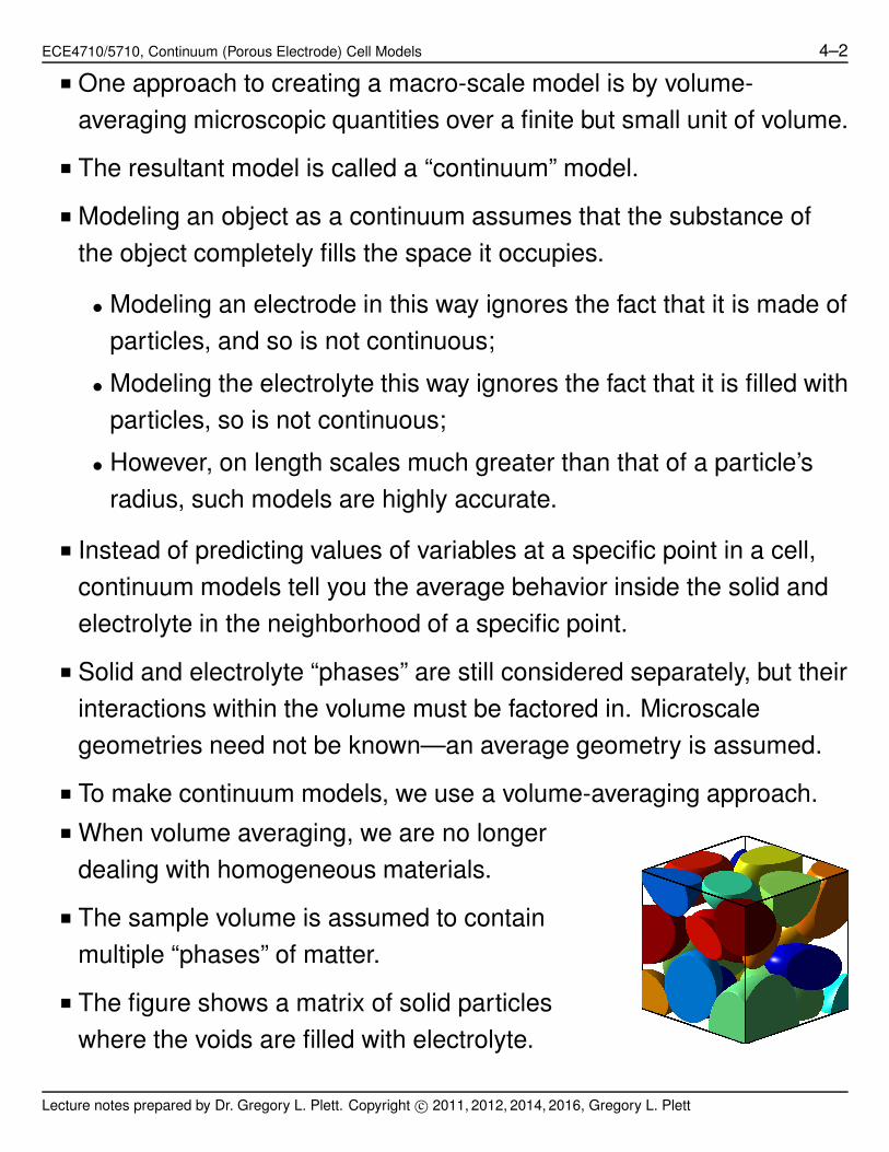
■ When volume averaging, we are no longer
dealing with homogeneous materials.
■ The sample volume is assumed to contain
multiple “phases” of matter.
■ The figure shows a matrix of solid particles
where the voids are filled with electrolyte.
Lecture notes prepared by Dr. Gregory L. Plett. Copyright c⃝ 2011, 2012, 2014, 2016, Gregory L. Plett
ECE4710/5710, Continuum (Porous Electrode) Cell Models 4–3
■ When we compute volume-average equations, we need to take the
multi-phase nature of the sample volume into account.
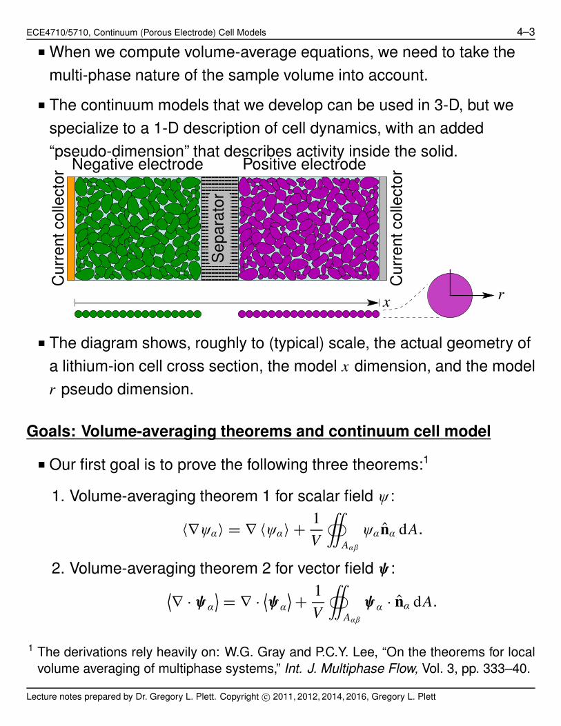
■ The continuum models that we develop can be used in 3-D, but we
specialize to a 1-D description of cell dynamics, with an added
“pseudo-dimension” that describes activity inside the solid.Negative electrode Positive electrode
Cu
rre
ntco
llect
or
Cu
rre
ntco
llect
or
Se
pa
rato
r
x r
■ The diagram shows, roughly to (typical) scale, the actual geometry of
a lithium-ion cell cross section, the model x dimension, and the model
r pseudo dimension.
Goals: Volume-averaging theorems and continuum cell model
■ Our first goal is to prove the following three theorems:1
1. Volume-averaging theorem 1 for scalar field ψ :
⟨∇ψα⟩ = ∇ ⟨ψα⟩ +1
V
‹
Aαβ
ψαnα dA.
2. Volume-averaging theorem 2 for vector field ψ :
⟨
∇ · ψα
⟩
= ∇ ·⟨
ψα
⟩
+1
V
‹
Aαβ
ψα · nα dA.
1 The derivations rely heavily on: W.G. Gray and P.C.Y. Lee, “On the theorems for localvolume averaging of multiphase systems,” Int. J. Multiphase Flow, Vol. 3, pp. 333–40.
Lecture notes prepared by Dr. Gregory L. Plett. Copyright c⃝ 2011, 2012, 2014, 2016, Gregory L. Plett
ECE4710/5710, Continuum (Porous Electrode) Cell Models 4–4
3. Volume-averaging theorem 3 for scalar field ψ :⟨
∂ψα
∂t
⟩
=∂ ⟨ψα⟩
∂t−
1
V
‹
Aαβ
ψαvαβ · nα dA.
■ Then, we will apply these volume-averaging theorems to the
microscale models from the prior chapter of notes to derive:
1. The volume-average approximation for charge conservation in the
solid phase of the porous electrode, which is
∇ · (σeff∇φs) = as F j .
2. The solid-phase mass-conservation equation,
∂cs
∂t=
1
r2
∂
∂r
(
Dsr2∂cs
∂r
)
.
3. The volume-average approximation for charge conservation in the
electrolyte phase of the porous electrode, which is
∇ ·(
κeff∇φe + κD,eff∇ ln ce
)
+ as F j = 0.
4. The volume-average approximation for mass conservation in the
electrolyte phase of the porous electrode, which is
∂(εece)
∂t= ∇ · (De,eff∇ ce) + as(1 − t0
+) j .
5. The volume-average approximation to the microscopic Butler–
Volmer kinetics relationship, j = j (cs,e, ce, φs, φe).
Lecture notes prepared by Dr. Gregory L. Plett. Copyright c⃝ 2011, 2012, 2014, 2016, Gregory L. Plett
ECE4710/5710, Continuum (Porous Electrode) Cell Models 4–5
4.2: Indicator and Dirac delta functions
■ We begin by deriving the volume-averaging theorems.
■ The sample volume is divided into two phases: the phase of interest
is denoted α; all other phase(s) are lumped into β.
■ Our goal is to find the average value of some variable in phase α.
■ To help with notation, we define an indicator function for phase α as
γα(x, y, z, t) =
⎧
⎨
⎩
1, if point (x, y, z) is in phase α at time t ;
0, otherwise.
■ We will need to take derivatives of γα, which are zero everywhere
except at the α–β phase boundaries.
■ But, how do we evaluate the derivative right on the boundary?
The Dirac delta function
■ To explore this, we introduce the Dirac delta function δ(x, y, z, t).
■ This function is unusual—it is defined in terms of its properties rather
than by stating exactly its value. These properties are:
δ(x, y, z, t) = 0, (x, y, z) = 0.˚
V
δ(x, y, z, t) dV = 1.
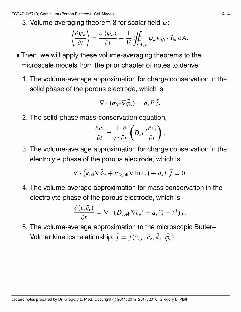
■ This is not an ordinary kind of function. It is a generalized function,
which can have many different but equivalent equations describing it.■ In one dimension, an example definition is
δ(x) = limϵ→0
⎧
⎨
⎩
1
ϵ, |x | ≤ ϵ/2;
0, otherwise.
Candidate δ(t)
−ϵ/2 ϵ/2
1/ϵ
Lecture notes prepared by Dr. Gregory L. Plett. Copyright c⃝ 2011, 2012, 2014, 2016, Gregory L. Plett
ECE4710/5710, Continuum (Porous Electrode) Cell Models 4–6
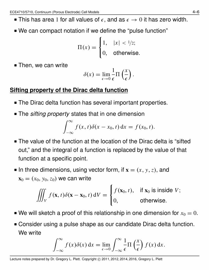
■ This has area 1 for all values of ϵ, and as ϵ → 0 it has zero width.
■ We can compact notation if we define the “pulse function”
,(x) =
⎧
⎨
⎩
1, |x | < 1/2;
0, otherwise.
■ Then, we can write
δ(x) = limϵ→0
1
ϵ,
(x
ϵ
)
.
Sifting property of the Dirac delta function
■ The Dirac delta function has several important properties.
■ The sifting property states that in one dimensionˆ ∞
−∞
f (x, t)δ(x − x0, t) dx = f (x0, t).
■ The value of the function at the location of the Dirac delta is “sifted
out,” and the integral of a function is replaced by the value of that
function at a specific point.
■ In three dimensions, using vector form, if x = (x, y, z), and
x0 = (x0, y0, z0) we can write
˚
V
f (x, t)δ(x − x0, t) dV =
⎧
⎨
⎩
f (x0, t), if x0 is inside V ;
0, otherwise.
■ We will sketch a proof of this relationship in one dimension for x0 = 0.
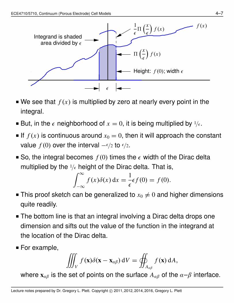
■ Consider using a pulse shape as our candidate Dirac delta function.
We writeˆ ∞
−∞
f (x)δ(x) dx = limϵ→0
ˆ ∞
−∞
1
ϵ,
(x
ϵ
)
f (x) dx .
Lecture notes prepared by Dr. Gregory L. Plett. Copyright c⃝ 2011, 2012, 2014, 2016, Gregory L. Plett
ECE4710/5710, Continuum (Porous Electrode) Cell Models 4–7
ϵ
Height: f (0); width ϵ
,(x
ϵ
)
f (x)
1
ϵ,
(x
ϵ
)
f (x)f (x)
Integrand is shadedarea divided by ϵ
■ We see that f (x) is multiplied by zero at nearly every point in the
integral.
■ But, in the ϵ neighborhood of x = 0, it is being multiplied by 1/ϵ.
■ If f (x) is continuous around x0 = 0, then it will approach the constant
value f (0) over the interval −ϵ/2 to ϵ/2.
■ So, the integral becomes f (0) times the ϵ width of the Dirac delta
multiplied by the 1/ϵ height of the Dirac delta. That is,ˆ ∞
−∞
f (x)δ(x) dx =1
ϵϵ f (0) = f (0).
■ This proof sketch can be generalized to x0 = 0 and higher dimensions
quite readily.
■ The bottom line is that an integral involving a Dirac delta drops one
dimension and sifts out the value of the function in the integrand at
the location of the Dirac delta.
■ For example,˚
V
f (x)δ(x − xαβ) dV =
‹
Aαβ
f (x) dA,
where xαβ is the set of points on the surface Aαβ of the α–β interface.
Lecture notes prepared by Dr. Gregory L. Plett. Copyright c⃝ 2011, 2012, 2014, 2016, Gregory L. Plett
ECE4710/5710, Continuum (Porous Electrode) Cell Models 4–8
4.3: Gradient of an indicator function
Running integral of a Dirac delta function
■ Now, consider integrating a 1-D Dirac delta from −∞ to x .
■ That is, we wish to computeˆ x
−∞
δ(χ) dχ .
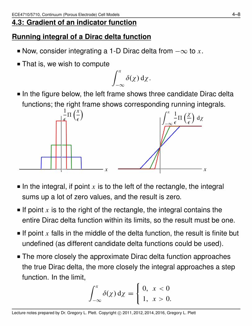
■ In the figure below, the left frame shows three candidate Dirac delta
functions; the right frame shows corresponding running integrals.
x
1
ϵ,
(x
ϵ
)
x
ˆ x
−∞
1
ϵ,
(χ
ϵ
)
dχ
■ In the integral, if point x is to the left of the rectangle, the integral
sums up a lot of zero values, and the result is zero.
■ If point x is to the right of the rectangle, the integral contains the
entire Dirac delta function within its limits, so the result must be one.
■ If point x falls in the middle of the delta function, the result is finite but
undefined (as different candidate delta functions could be used).
■ The more closely the approximate Dirac delta function approaches
the true Dirac delta, the more closely the integral approaches a step
function. In the limit,ˆ x
−∞
δ(χ) dχ =
{
0, x < 0
1, x > 0.
Lecture notes prepared by Dr. Gregory L. Plett. Copyright c⃝ 2011, 2012, 2014, 2016, Gregory L. Plett
ECE4710/5710, Continuum (Porous Electrode) Cell Models 4–9
■ That is, the running integral of a Dirac delta function is a step function.
■ Also, the derivative of a step function is the Dirac delta function.
Gradient of the indicator function
■ Now, we get to the reason for introducing the Dirac delta function: We
need to be able to represent the gradient of the indicator function.
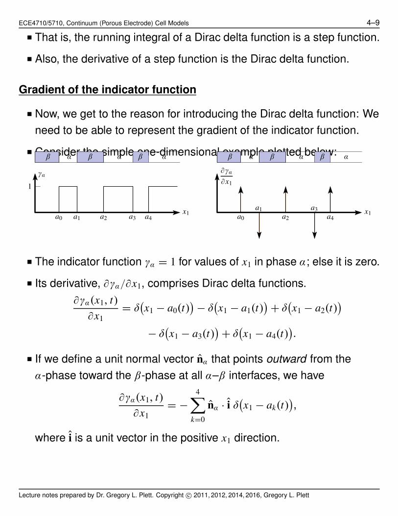
■ Consider the simple one-dimensional example plotted below:
γα∂γα
∂x1
x1 x1
β βββ ββ α ααα αα
1
a0 a0a1 a2a2 a3 a4 a4
a1 a3
■ The indicator function γα = 1 for values of x1 in phase α; else it is zero.
■ Its derivative, ∂γα/∂x1, comprises Dirac delta functions.
∂γα(x1, t)
∂x1
= δ(
x1 − a0(t))
− δ(
x1 − a1(t))
+ δ(
x1 − a2(t))
− δ(
x1 − a3(t))
+ δ(
x1 − a4(t))
.
■ If we define a unit normal vector nα that points outward from the
α-phase toward the β-phase at all α–β interfaces, we have
∂γα(x1, t)
∂x1
= −
4∑
k=0
nα · i δ(
x1 − ak(t))
,
where i is a unit vector in the positive x1 direction.
Lecture notes prepared by Dr. Gregory L. Plett. Copyright c⃝ 2011, 2012, 2014, 2016, Gregory L. Plett
ECE4710/5710, Continuum (Porous Electrode) Cell Models 4–10
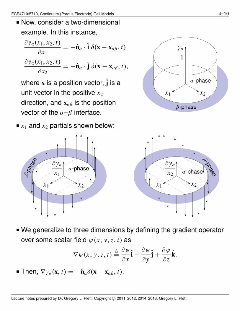
■ Now, consider a two-dimensional
example. In this instance,
∂γα(x1, x2, t)
∂x1
= −nα · i δ(x − xαβ, t)
∂γα(x1, x2, t)
∂x2
= −nα · j δ(x − xαβ, t),
where x is a position vector, j is a
unit vector in the positive x2
direction, and xαβ is the position
vector of the α–β interface.
■ x1 and x2 partials shown below:
β-phase
α-phase
γα
1
x1 x2
β-p
hase
α-phase
x1 x2
∂γα
x1
β-phaseα-phase
x1 x2
∂γα
x2
■ We generalize to three dimensions by defining the gradient operator
over some scalar field ψ(x, y, z, t) as
∇ψ(x, y, z, t)△=∂ψ
∂xi +
∂ψ
∂yj +
∂ψ
∂zk.
■ Then, ∇γα(x, t) = −nαδ(x − xαβ, t).
Lecture notes prepared by Dr. Gregory L. Plett. Copyright c⃝ 2011, 2012, 2014, 2016, Gregory L. Plett
ECE4710/5710, Continuum (Porous Electrode) Cell Models 4–11
4.4: Phase and intrinsic averages
■ When applying averaging techniques to obtain continuum equations,
it is necessary to select an averaging volume that will result in
meaningful averages.
■ This can be met when the characteristic length of the averaging
volume is much greater than the pore openings (between particles),
but much less than the electrode length.
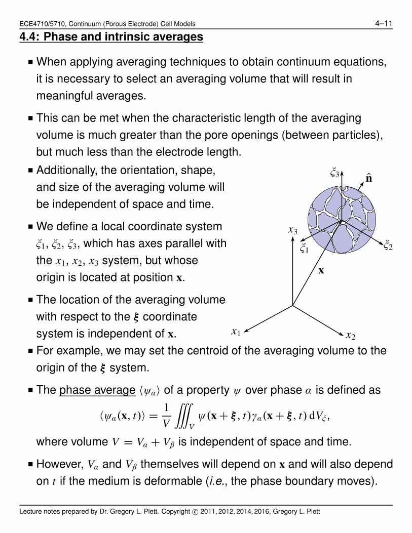
■ Additionally, the orientation, shape,
and size of the averaging volume will
be independent of space and time.
■ We define a local coordinate system
ξ1, ξ2, ξ3, which has axes parallel with
the x1, x2, x3 system, but whose
origin is located at position x.
■ The location of the averaging volume
with respect to the ξ coordinate
system is independent of x. x1 x2
x3
x
ξ1ξ2
ξ3 n
■ For example, we may set the centroid of the averaging volume to the
origin of the ξ system.
■ The phase average ⟨ψα⟩ of a property ψ over phase α is defined as
⟨ψα(x, t)⟩ =1
V
˚
V
ψ(x + ξ , t)γα(x + ξ , t) dVξ ,
where volume V = Vα + Vβ is independent of space and time.
■ However, Vα and Vβ themselves will depend on x and will also depend
on t if the medium is deformable (i.e., the phase boundary moves).
Lecture notes prepared by Dr. Gregory L. Plett. Copyright c⃝ 2011, 2012, 2014, 2016, Gregory L. Plett
ECE4710/5710, Continuum (Porous Electrode) Cell Models 4–12
■ Physically, the phase average is a property of the α-phase only
averaged over the entire volume occupied by both the α- and
β-phases in the averaging volume.
■ Note that we could also write this integral as
⟨ψα(x, t)⟩ =1
V
˚
Vα(x,t)
ψ(x + ξ , t) dVξ ,
but this is less useful since the limits of integration depend on spatial
location and on time if the medium deforms.
■ The intrinsic phase average ψα of a property ψ over phase α is
ψα(x, t) =1
Vα(x, t)
˚
Vα(x,t)
ψ(x + ξ , t) dVξ .
■ It describes a property of the α-phase averaged over that phase only.
■ Comparing the two types of phase average, we see
⟨ψα(x, t)⟩ = εα(x, t)ψα(x, t), or ψα(x, t) =1
εα(x, t)⟨ψα(x, t)⟩ ,
where the volume fraction of the α-phase is defined as
εα(x, t) =Vα(x, t)
V=
1
V
˚
V
γα(x + ξ , t) dVξ .
EXAMPLE: Consider a rock-filled beaker, where εs = 0.5, and a second
electrolyte-filled beaker having salt concentration 1000 mol m−3. We
pour electrolyte into the first beaker until it is full, so εe = 0.5.
■ Taking a phase average of salt concentration in the porous media,
⟨ce⟩ =1
V
˚
Ve
ce(x + ξ , t) dVξ = ce
Ve
V= 0.5ce = 500 mol m−3.
■ Taking an intrinsic phase average of the salt concentration instead
ce =1
Ve
˚
Ve
ce(x + ξ , t) dVξ = ce
Ve
Ve
= ce = 1000 mol m−3.
Lecture notes prepared by Dr. Gregory L. Plett. Copyright c⃝ 2011, 2012, 2014, 2016, Gregory L. Plett
ECE4710/5710, Continuum (Porous Electrode) Cell Models 4–13
■ The phase average tells us, from the perspective of the entire
volume, what is the concentration of salt in the volume.
■ The intrinsic phase average tells us, from the perspective of the
solution within the volume, the concentration of salt in the solution.
■ Intrinsic phase average is directly related to micro-scale models
where physical measurements are made, so is the one we will use.
■ But, we will derive our equations in terms of the phase average
(easier), and convert to intrinsic phase averages when finished.
■ Before proceeding with the averaging theorems, we examine a useful
identity involving the gradient operator.
• Define ∇x to refer to the gradient taken with respect to the x
coordinates, holding ξ1, ξ2, and ξ3 constant;
• Define ∇ξ to refer to the gradient taken with respect to the ξ
coordinates, holding x1, x2, and x3 constant;
• Define ∇ to refer to either ∇x or ∇ξ .
■ If a function is symmetrically dependent on x and ξ (i.e., it depends
on x + ξ rather than on x and ξ ) the gradient in the x-coordinate
system is equal to the gradient in the ξ -coordinate system:
∇xψ(x + ξ , t) = ∇ξψ(x + ξ , t) = ∇ψ(x + ξ , t)
∇xγα(x + ξ , t) = ∇ξγα(x + ξ , t) = ∇γα(x + ξ , t).
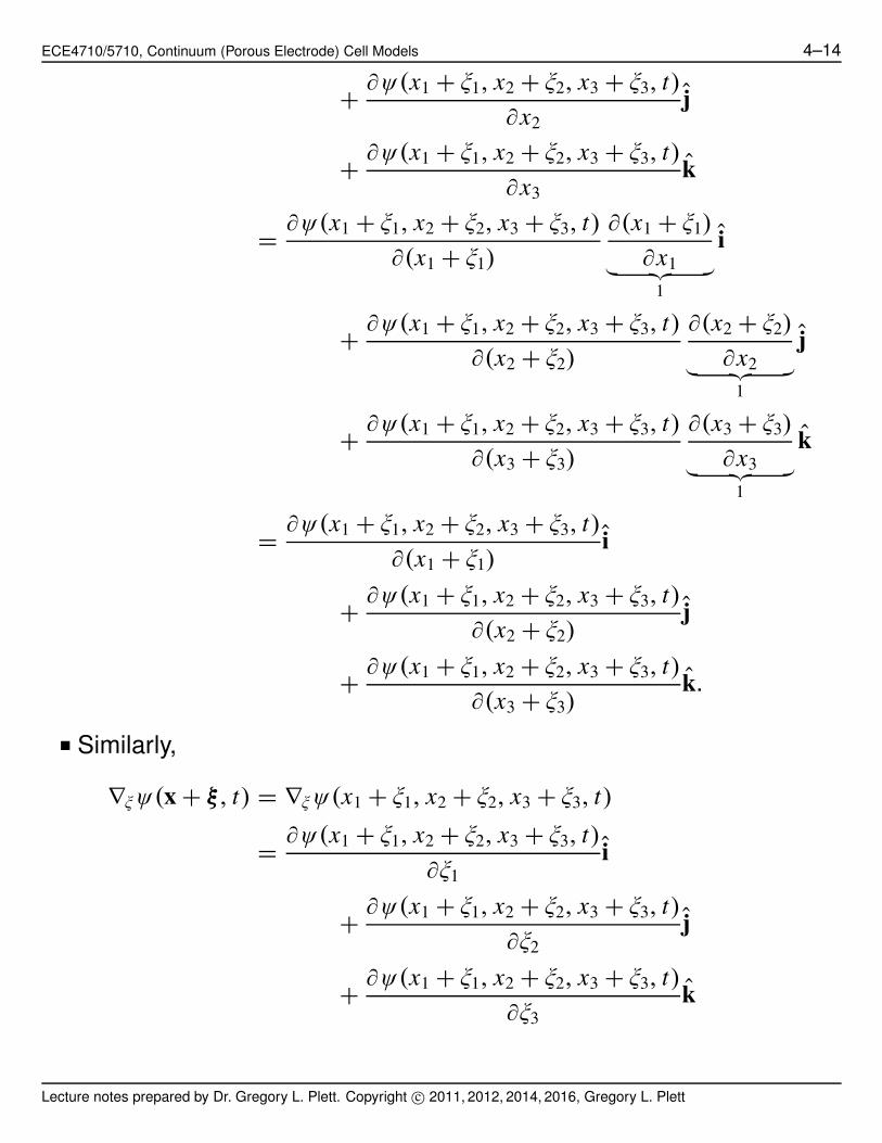
PROOF: Consider
∇xψ(x + ξ , t) = ∇xψ(x1 + ξ1, x2 + ξ2, x3 + ξ3, t)
=∂ψ(x1 + ξ1, x2 + ξ2, x3 + ξ3, t)
∂x1
i
Lecture notes prepared by Dr. Gregory L. Plett. Copyright c⃝ 2011, 2012, 2014, 2016, Gregory L. Plett
ECE4710/5710, Continuum (Porous Electrode) Cell Models 4–14
+∂ψ(x1 + ξ1, x2 + ξ2, x3 + ξ3, t)
∂x2
j
+∂ψ(x1 + ξ1, x2 + ξ2, x3 + ξ3, t)
∂x3
k
=∂ψ(x1 + ξ1, x2 + ξ2, x3 + ξ3, t)
∂(x1 + ξ1)
∂(x1 + ξ1)
∂x1︸ ︷︷ ︸
1
i
+∂ψ(x1 + ξ1, x2 + ξ2, x3 + ξ3, t)
∂(x2 + ξ2)
∂(x2 + ξ2)
∂x2︸ ︷︷ ︸
1
j
+∂ψ(x1 + ξ1, x2 + ξ2, x3 + ξ3, t)
∂(x3 + ξ3)
∂(x3 + ξ3)
∂x3︸ ︷︷ ︸
1
k
=∂ψ(x1 + ξ1, x2 + ξ2, x3 + ξ3, t)
∂(x1 + ξ1)i
+∂ψ(x1 + ξ1, x2 + ξ2, x3 + ξ3, t)
∂(x2 + ξ2)j
+∂ψ(x1 + ξ1, x2 + ξ2, x3 + ξ3, t)
∂(x3 + ξ3)k.
■ Similarly,
∇ξψ(x + ξ , t) = ∇ξψ(x1 + ξ1, x2 + ξ2, x3 + ξ3, t)
=∂ψ(x1 + ξ1, x2 + ξ2, x3 + ξ3, t)
∂ξ1
i
+∂ψ(x1 + ξ1, x2 + ξ2, x3 + ξ3, t)
∂ξ2
j
+∂ψ(x1 + ξ1, x2 + ξ2, x3 + ξ3, t)
∂ξ3
k
Lecture notes prepared by Dr. Gregory L. Plett. Copyright c⃝ 2011, 2012, 2014, 2016, Gregory L. Plett
ECE4710/5710, Continuum (Porous Electrode) Cell Models 4–15
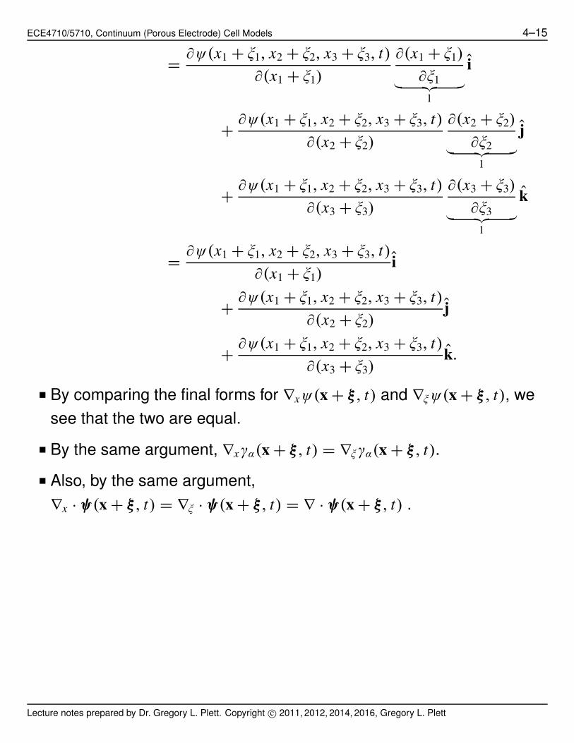
=∂ψ(x1 + ξ1, x2 + ξ2, x3 + ξ3, t)
∂(x1 + ξ1)
∂(x1 + ξ1)
∂ξ1︸ ︷︷ ︸
1
i
+∂ψ(x1 + ξ1, x2 + ξ2, x3 + ξ3, t)
∂(x2 + ξ2)
∂(x2 + ξ2)
∂ξ2︸ ︷︷ ︸
1
j
+∂ψ(x1 + ξ1, x2 + ξ2, x3 + ξ3, t)
∂(x3 + ξ3)
∂(x3 + ξ3)
∂ξ3︸ ︷︷ ︸
1
k
=∂ψ(x1 + ξ1, x2 + ξ2, x3 + ξ3, t)
∂(x1 + ξ1)i
+∂ψ(x1 + ξ1, x2 + ξ2, x3 + ξ3, t)
∂(x2 + ξ2)j
+∂ψ(x1 + ξ1, x2 + ξ2, x3 + ξ3, t)
∂(x3 + ξ3)k.
■ By comparing the final forms for ∇xψ(x + ξ , t) and ∇ξψ(x + ξ , t), we
see that the two are equal.
■ By the same argument, ∇xγα(x + ξ , t) = ∇ξγα(x + ξ , t).
■ Also, by the same argument,
∇x · ψ(x + ξ , t) = ∇ξ · ψ(x + ξ , t) = ∇ · ψ(x + ξ , t) .
Lecture notes prepared by Dr. Gregory L. Plett. Copyright c⃝ 2011, 2012, 2014, 2016, Gregory L. Plett
ECE4710/5710, Continuum (Porous Electrode) Cell Models 4–16
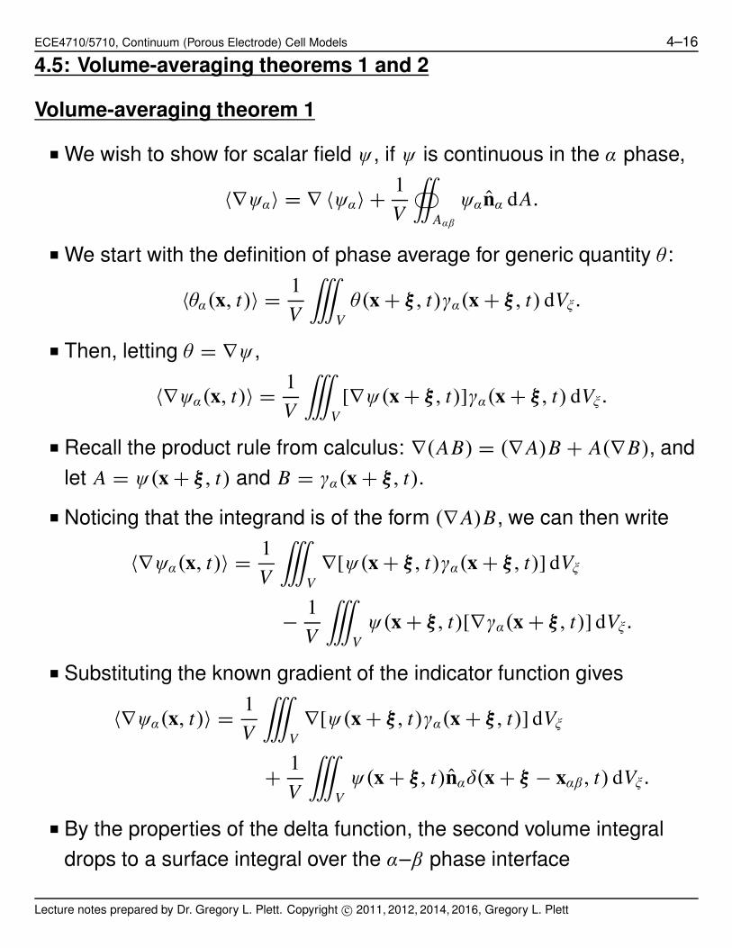
4.5: Volume-averaging theorems 1 and 2
Volume-averaging theorem 1
■ We wish to show for scalar field ψ , if ψ is continuous in the α phase,
⟨∇ψα⟩ = ∇ ⟨ψα⟩ +1
V
‹
Aαβ
ψαnα dA.
■ We start with the definition of phase average for generic quantity θ :
⟨θα(x, t)⟩ =1
V
˚
V
θ(x + ξ , t)γα(x + ξ , t) dVξ .
■ Then, letting θ = ∇ψ ,
⟨∇ψα(x, t)⟩ =1
V
˚
V
[∇ψ(x + ξ , t)]γα(x + ξ , t) dVξ .
■ Recall the product rule from calculus: ∇(AB) = (∇ A)B + A(∇ B), and
let A = ψ(x + ξ , t) and B = γα(x + ξ , t).
■ Noticing that the integrand is of the form (∇ A)B, we can then write
⟨∇ψα(x, t)⟩ =1
V
˚
V
∇[ψ(x + ξ , t)γα(x + ξ , t)] dVξ
−1
V
˚
V
ψ(x + ξ , t)[∇γα(x + ξ , t)] dVξ .
■ Substituting the known gradient of the indicator function gives
⟨∇ψα(x, t)⟩ =1
V
˚
V
∇[ψ(x + ξ , t)γα(x + ξ , t)] dVξ
+1
V
˚
V
ψ(x + ξ , t)nαδ(x + ξ − xαβ, t) dVξ .
■ By the properties of the delta function, the second volume integral
drops to a surface integral over the α–β phase interface
Lecture notes prepared by Dr. Gregory L. Plett. Copyright c⃝ 2011, 2012, 2014, 2016, Gregory L. Plett

ECE4710/5710, Continuum (Porous Electrode) Cell Models 4–17
1
V
˚
V
ψ(x + ξ , t)nαδ(x + ξ − xαβ, t) dVξ =1
V
‹
Aαβ
ψα(x + ξ , t)nα dA,
and we get
⟨∇ψα(x, t)⟩ =1
V
˚
V
∇[ψ(x + ξ , t)γα(x + ξ , t)] dVξ
+1
V
‹
Aαβ
ψα(x + ξ , t)nα dA.
■ We consider ∇ = ∇x on the RHS, so it may be removed from the
integral because V is independent of x. Thus, we obtain
⟨∇ψα⟩ = ∇
[
1
V
˚
V
ψ(x + ξ , t)γα(x + ξ , t) dVξ
]
+1
V
‹
Aαβ
ψα(x + ξ , t)nα dA
⟨∇ψα⟩ = ∇ ⟨ψα⟩ +1
V
‹
Aαβ
ψαnα dA,
which proves volume averaging theorem 1.
INTERPRETATION: Volume average of gradient = gradient of volume
average plus correction term.
■ Correction sums up scaled vectors pointing away from the α–β
interface. Result points in the direction of largest surface field.
■ By extension, we can find the intrinsic phase average
∇ψα =1
εα⟨∇ψα⟩ =
1
εα
[
∇ ⟨ψα⟩ +1
V
‹
Aαβ
ψαnα dA
]
=1
εα
[
∇(
εαψα)
+1
V
‹
Aαβ
ψαnα dA
]
.
Lecture notes prepared by Dr. Gregory L. Plett. Copyright c⃝ 2011, 2012, 2014, 2016, Gregory L. Plett
ECE4710/5710, Continuum (Porous Electrode) Cell Models 4–18
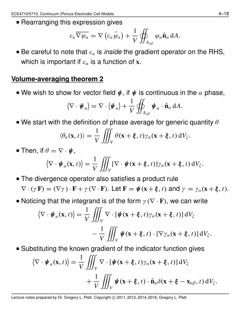
■ Rearranging this expression gives
εα∇ψα = ∇(
εαψα)
+1
V
‹
Aαβ
ψαnα dA.
■ Be careful to note that εα is inside the gradient operator on the RHS,
which is important if εα is a function of x.
Volume-averaging theorem 2
■ We wish to show for vector field ψ , if ψ is continuous in the α phase,⟨
∇ · ψα
⟩
= ∇ ·⟨
ψα
⟩
+1
V
‹
Aαβ
ψα · nα dA.
■ We start with the definition of phase average for generic quantity θ
⟨θα(x, t)⟩ =1
V
˚
V
θ(x + ξ , t)γα(x + ξ , t) dVξ .
■ Then, if θ = ∇ · ψ ,⟨
∇ · ψα(x, t)⟩
=1
V
˚
V
[∇ · ψ(x + ξ , t)]γα(x + ξ , t) dVξ .
■ The divergence operator also satisfies a product rule
∇ · (γF) = (∇γ ) · F + γ (∇ · F). Let F = ψ(x + ξ , t) and γ = γα(x + ξ , t).
■ Noticing that the integrand is of the form γ (∇ · F), we can write⟨
∇ · ψα(x, t)⟩
=1
V
˚
V
∇ · [ψ(x + ξ , t)γα(x + ξ , t)] dVξ
−1
V
˚
V
ψ(x + ξ , t) · [∇γα(x + ξ , t)] dVξ .
■ Substituting the known gradient of the indicator function gives⟨
∇ · ψα(x, t)⟩
=1
V
˚
V
∇ · [ψ(x + ξ , t)γα(x + ξ , t)] dVξ
+1
V
˚
V
ψ(x + ξ , t) · nαδ(x + ξ − xαβ, t) dVξ .
Lecture notes prepared by Dr. Gregory L. Plett. Copyright c⃝ 2011, 2012, 2014, 2016, Gregory L. Plett
ECE4710/5710, Continuum (Porous Electrode) Cell Models 4–19
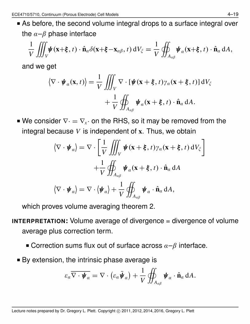
■ As before, the second volume integral drops to a surface integral over
the α–β phase interface
1
V
˚
V
ψ(x+ξ , t) · nαδ(x+ξ−xαβ, t) dVξ =1
V
‹
Aαβ
ψα(x+ξ , t) · nα dA,
and we get
⟨
∇ · ψα(x, t)⟩
=1
V
˚
V
∇ · [ψ(x + ξ , t)γα(x + ξ , t)] dVξ
+1
V
‹
Aαβ
ψα(x + ξ , t) · nα dA.
■ We consider ∇· = ∇x · on the RHS, so it may be removed from the
integral because V is independent of x. Thus, we obtain
⟨
∇ · ψα
⟩
= ∇ ·
[
1
V
˚
V
ψ(x + ξ , t)γα(x + ξ , t) dVξ
]
+1
V
‹
Aαβ
ψα(x + ξ , t) · nα dA
⟨
∇ · ψα
⟩
= ∇ ·⟨
ψα
⟩
+1
V
‹
Aαβ
ψα · nα dA,
which proves volume averaging theorem 2.
INTERPRETATION: Volume average of divergence = divergence of volume
average plus correction term.
■ Correction sums flux out of surface across α–β interface.
■ By extension, the intrinsic phase average is
εα∇ · ψα = ∇ ·(
εαψα
)
+1
V
‹
Aαβ
ψα · nα dA.
Lecture notes prepared by Dr. Gregory L. Plett. Copyright c⃝ 2011, 2012, 2014, 2016, Gregory L. Plett
ECE4710/5710, Continuum (Porous Electrode) Cell Models 4–20
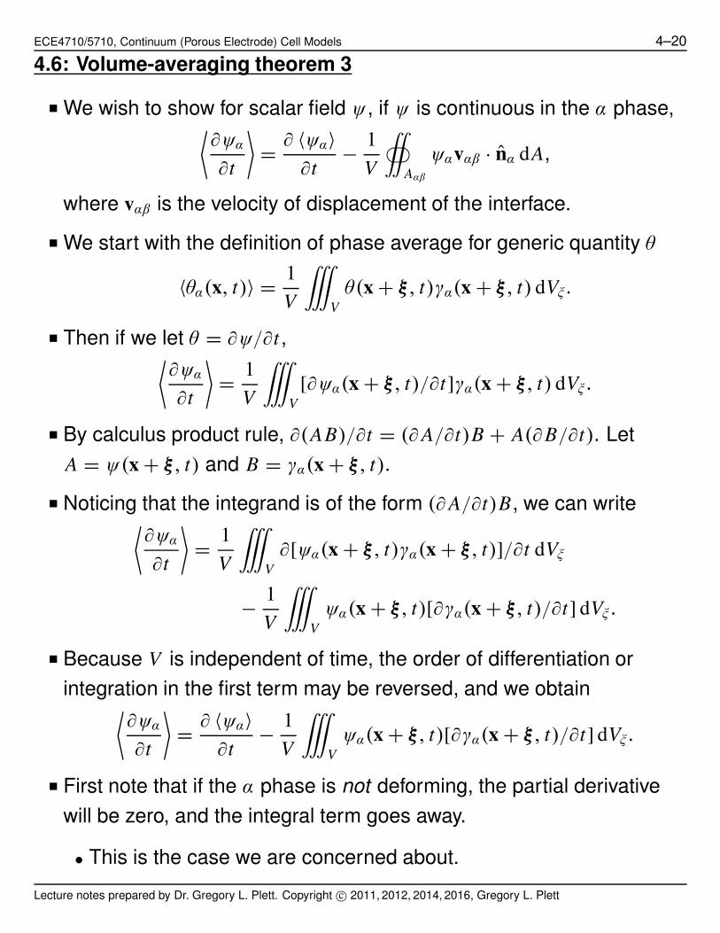
4.6: Volume-averaging theorem 3
■ We wish to show for scalar field ψ , if ψ is continuous in the α phase,⟨
∂ψα
∂t
⟩
=∂ ⟨ψα⟩
∂t−
1
V
‹
Aαβ
ψαvαβ · nα dA,
where vαβ is the velocity of displacement of the interface.
■ We start with the definition of phase average for generic quantity θ
⟨θα(x, t)⟩ =1
V
˚
V
θ(x + ξ , t)γα(x + ξ , t) dVξ .
■ Then if we let θ = ∂ψ/∂t ,⟨
∂ψα
∂t
⟩
=1
V
˚
V
[∂ψα(x + ξ , t)/∂t]γα(x + ξ , t) dVξ .
■ By calculus product rule, ∂(AB)/∂t = (∂A/∂t)B + A(∂B/∂t). Let
A = ψ(x + ξ , t) and B = γα(x + ξ , t).
■ Noticing that the integrand is of the form (∂A/∂t)B, we can write⟨
∂ψα
∂t
⟩
=1
V
˚
V
∂[ψα(x + ξ , t)γα(x + ξ , t)]/∂t dVξ
−1
V
˚
V
ψα(x + ξ , t)[∂γα(x + ξ , t)/∂t] dVξ .
■ Because V is independent of time, the order of differentiation or
integration in the first term may be reversed, and we obtain⟨
∂ψα
∂t
⟩
=∂ ⟨ψα⟩
∂t−
1
V
˚
V
ψα(x + ξ , t)[∂γα(x + ξ , t)/∂t] dVξ .
■ First note that if the α phase is not deforming, the partial derivative
will be zero, and the integral term goes away.
• This is the case we are concerned about.
Lecture notes prepared by Dr. Gregory L. Plett. Copyright c⃝ 2011, 2012, 2014, 2016, Gregory L. Plett
ECE4710/5710, Continuum (Porous Electrode) Cell Models 4–21
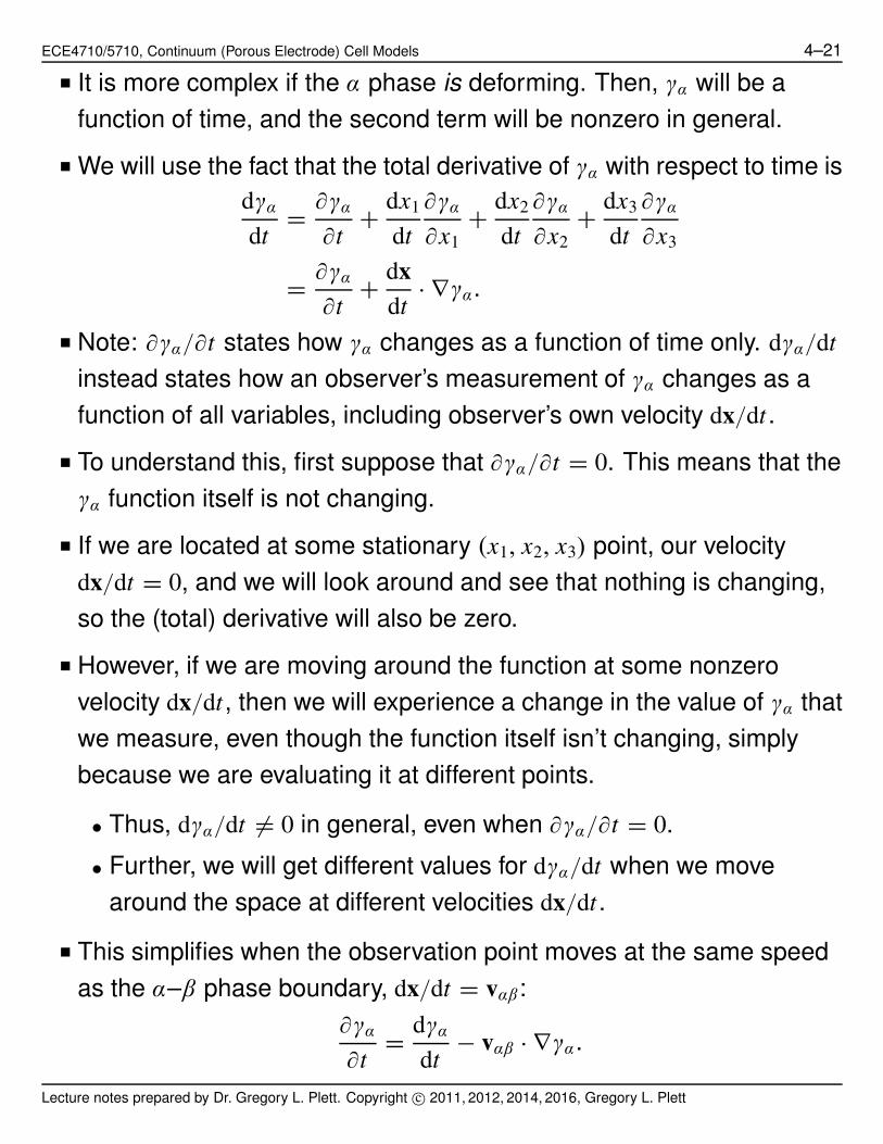
■ It is more complex if the α phase is deforming. Then, γα will be a
function of time, and the second term will be nonzero in general.
■ We will use the fact that the total derivative of γα with respect to time is
dγα
dt=∂γα
∂t+
dx1
dt
∂γα
∂x1
+dx2
dt
∂γα
∂x2
+dx3
dt
∂γα
∂x3
=∂γα
∂t+
dx
dt· ∇γα.
■ Note: ∂γα/∂t states how γα changes as a function of time only. dγα/dt
instead states how an observer’s measurement of γα changes as a
function of all variables, including observer’s own velocity dx/dt .
■ To understand this, first suppose that ∂γα/∂t = 0. This means that the
γα function itself is not changing.
■ If we are located at some stationary (x1, x2, x3) point, our velocity
dx/dt = 0, and we will look around and see that nothing is changing,
so the (total) derivative will also be zero.
■ However, if we are moving around the function at some nonzero
velocity dx/dt , then we will experience a change in the value of γα that
we measure, even though the function itself isn’t changing, simply
because we are evaluating it at different points.
• Thus, dγα/dt = 0 in general, even when ∂γα/∂t = 0.
• Further, we will get different values for dγα/dt when we move
around the space at different velocities dx/dt .
■ This simplifies when the observation point moves at the same speed
as the α–β phase boundary, dx/dt = vαβ:
∂γα
∂t=
dγα
dt− vαβ · ∇γα.
Lecture notes prepared by Dr. Gregory L. Plett. Copyright c⃝ 2011, 2012, 2014, 2016, Gregory L. Plett
ECE4710/5710, Continuum (Porous Electrode) Cell Models 4–22
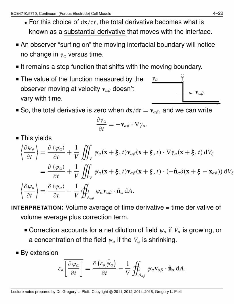
• For this choice of dx/dt , the total derivative becomes what is
known as a substantial derivative that moves with the interface.
■ An observer “surfing on” the moving interfacial boundary will notice
no change in γα versus time.
■ It remains a step function that shifts with the moving boundary.
■ The value of the function measured by the
observer moving at velocity vαβ doesn’t
vary with time.
γa
vαβ
■ So, the total derivative is zero when dx/dt = vαβ, and we can write
∂γα
∂t= −vαβ · ∇γα.
■ This yields⟨
∂ψα
∂t
⟩
=∂ ⟨ψα⟩
∂t+
1
V
˚
V
ψα(x + ξ , t)vαβ(x + ξ , t) · ∇γα(x + ξ , t) dVξ
=∂ ⟨ψα⟩
∂t+
1
V
˚
V
ψα(x + ξ , t)vαβ(x + ξ , t) · (−nαδ(x + ξ − xαβ)) dVξ
⟨
∂ψα
∂t
⟩
=∂ ⟨ψα⟩
∂t−
1
V
‹
Aαβ
ψαvαβ · nα dA.
INTERPRETATION: Volume average of time derivative = time derivative of
volume average plus correction term.
■ Correction accounts for a net dilution of field ψα if Vα is growing, or
a concentration of the field ψa if the Vα is shrinking.
■ By extension
εα
[
∂ψα
∂t
]
=∂
(
εαψα)
∂t−
1
V
‹
Aαβ
ψαvαβ · nα dA.
Lecture notes prepared by Dr. Gregory L. Plett. Copyright c⃝ 2011, 2012, 2014, 2016, Gregory L. Plett
ECE4710/5710, Continuum (Porous Electrode) Cell Models 4–23
4.7: Continuum models: Charge conservation in the solid
■ We now apply the volume-averaging theorems to develop continuum
model equivalents of the five microscale model equations.
■ Start with the microscale model of charge conservation in the solid,
∇ · (is) = ∇ · (−σ∇φs) = 0.
■ Using intrinsic averages and volume-averaging theorem 2
εs∇ · (−σ∇φs) = ∇ ·(
εs(−σ∇φs))
+1
V
‹
Ase
(−σ∇φs) · ns dA
0 = ∇ ·(
εs(−σ∇φs))
+1
V
‹
Ase
(−σ∇φs) · ns dA.
■ Let’s look at the integral term first. Note that we are integrating over
the solid-electrolyte boundary.
■ Last chapter, we noted the boundary condition for the charge
conservation equation; namely,
ns · σ∇φs = −F j .
ASSUME: That j is homogeneous, and that we can model j using
volume-averaged inputs.
1
V
‹
Ase
(−σ∇φs) · ns dA =1
V
‹
Ase
F j (cs, ce,φs,φe) dA
≈Ase
VF j (cs,e, ce, φs, φe)
≈ as F j (cs,e, ce, φs, φe) = as F j .
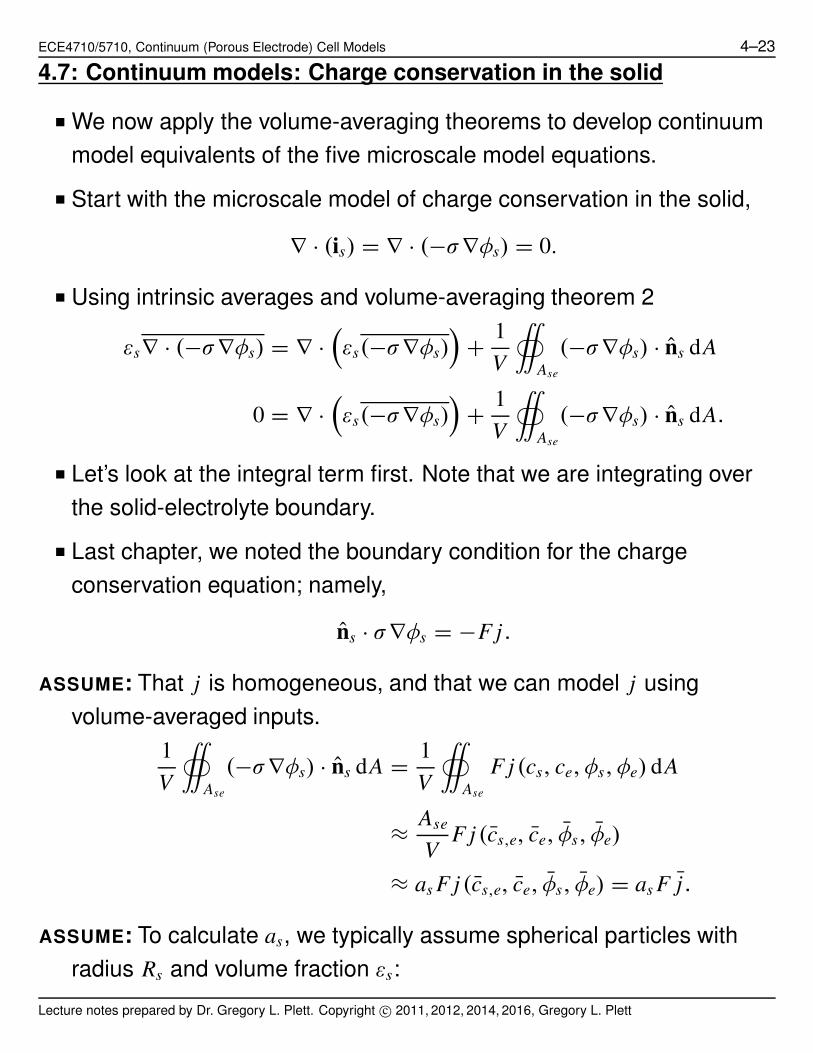
ASSUME: To calculate as, we typically assume spherical particles with
radius Rs and volume fraction εs:
Lecture notes prepared by Dr. Gregory L. Plett. Copyright c⃝ 2011, 2012, 2014, 2016, Gregory L. Plett
ECE4710/5710, Continuum (Porous Electrode) Cell Models 4–24
as =total surface area of spheres in volume
total volume of a sphere
= εs
4πR2s
43πR3
s
=3εs
Rs
.
■ So, we now have the result
0 = ∇ ·(
εs(−σ∇φs))
+ as F j
∇ ·(
εs(−σ∇φs))
= −as F j .
■ What to do with the (−σ∇φs) term? We might consider using
volume-averaging theorem 1, but note that we don’t know what φsns is
at the boundary, so are unable to evaluate this term.
ASSUME: Instead, it’s common to model εs(−σ∇φs) ≈ −σeff∇φs.
■ The effective conductivity σeff =εsσδ
τ, where δ < 1 is the
constrictivity of the and τ ≥ 1 is the tortuosity of the media.
■ That is, σ is the bulk conductivity of homogeneous materials, and
σeff is the effective conductivity of the solid in the porous media.
■ Note that σeff < σ since there are restrictions to flow of current.
■ It is frequently assumed that σeff = σεbrugs , where “brug” is
Bruggeman’s coefficient, and is normally assumed to take on the
value of 1.5, although other values may work better.
■ To get better value for σeff, we could do microscale simulations with
realistic particle geometries, or measure directly via experiment.
■ Collecting the above results, we now have the final continuum model
of charge conservation in the solid,
∇ · (−σeff∇φs) = −as F j .
Lecture notes prepared by Dr. Gregory L. Plett. Copyright c⃝ 2011, 2012, 2014, 2016, Gregory L. Plett
ECE4710/5710, Continuum (Porous Electrode) Cell Models 4–25
■ Also note that εs is = εs(−σ∇φs) = −σeff∇φs.
How well does the Bruggeman relationship work?
■ We now illustrate, by example, how well an effective property in a
volume-average equation can represent the effect of an intrinsic
property in a microscale equation.
■ We use the PDE simulation system COMSOL to help find results
(example is adapted from COMSOL documentation).
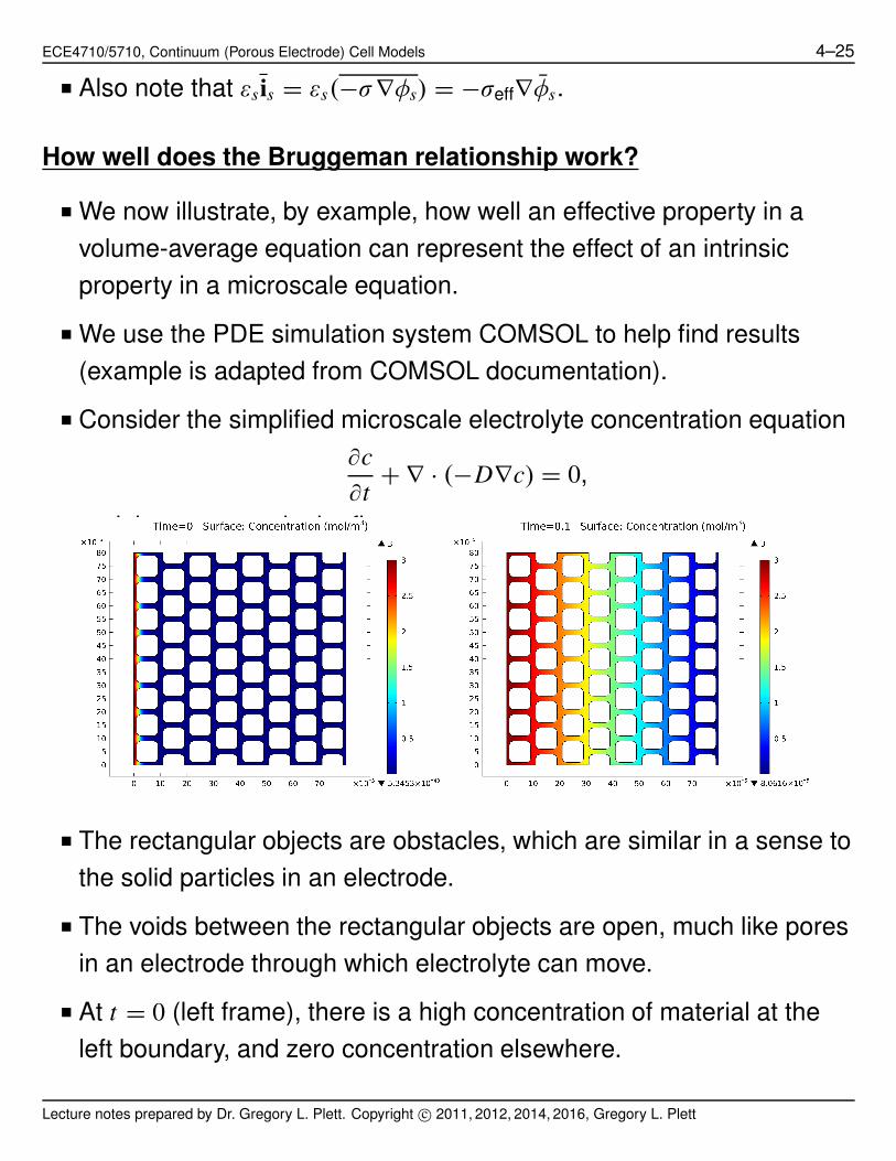
■ Consider the simplified microscale electrolyte concentration equation
∂c
∂t+ ∇ · (−D∇c) = 0,
and the geometry in the figure.
■ The rectangular objects are obstacles, which are similar in a sense to
the solid particles in an electrode.
■ The voids between the rectangular objects are open, much like pores
in an electrode through which electrolyte can move.
■ At t = 0 (left frame), there is a high concentration of material at the
left boundary, and zero concentration elsewhere.
Lecture notes prepared by Dr. Gregory L. Plett. Copyright c⃝ 2011, 2012, 2014, 2016, Gregory L. Plett
ECE4710/5710, Continuum (Porous Electrode) Cell Models 4–26
■ By time 0.1 s (right frame), there is a uniform concentration gradient
established through the porous structure, as indicated by the shading.
■ We’re interested in modeling the flux of material out the right edge. It
is zero at time t = 0, and increases to a steady-state value over time.
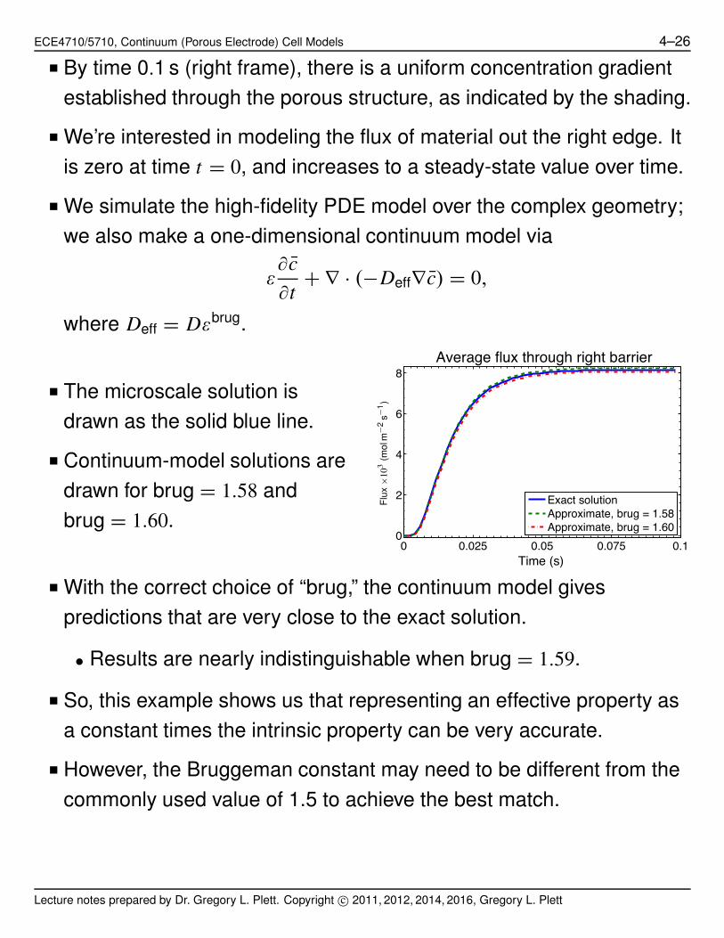
■ We simulate the high-fidelity PDE model over the complex geometry;
we also make a one-dimensional continuum model via
ε∂ c
∂t+ ∇ · (−Deff∇ c) = 0,
where Deff = Dεbrug.
■ The microscale solution is
drawn as the solid blue line.
■ Continuum-model solutions are
drawn for brug = 1.58 and
brug = 1.60.0 0.025 0.05 0.075 0.1
0
2
4
6
8
Time (s)
Average flux through right barrier
Exact solutionApproximate, brug = 1.58Approximate, brug = 1.60
Flu
x×
10
3(m
olm
−2
s−1)
■ With the correct choice of “brug,” the continuum model gives
predictions that are very close to the exact solution.
• Results are nearly indistinguishable when brug = 1.59.
■ So, this example shows us that representing an effective property as
a constant times the intrinsic property can be very accurate.
■ However, the Bruggeman constant may need to be different from the
commonly used value of 1.5 to achieve the best match.
Lecture notes prepared by Dr. Gregory L. Plett. Copyright c⃝ 2011, 2012, 2014, 2016, Gregory L. Plett
ECE4710/5710, Continuum (Porous Electrode) Cell Models 4–27
4.8: Mass conservation in the solid and electrolyte
Mass conservation in the solid
■ As mentioned earlier, our continuum model has spatial dimension(s)
plus a pseudo dimension.
■ This pseudo dimension represents what is happening at some point
inside a particle that resides at some spatial location.
• We could make a continuum model with three spatial dimensions
plus an additional pseudo dimension, resulting in a
pseudo-four-dimensional model. The math we develop here is
general enough to encompass this case, but
• We ultimately specialize to a model with one spatial dimension
plus the additional pseudo dimension, resulting in a
pseudo-two-dimensional model.
■ We assume that there is a particle centered at any spatial location,
that the particle is spherical, and that the concentration of lithium
within the particle is spherically symmetric.
■ So, to create the continuum equation for mass conservation within the
solid, we don’t need to use any volume-averaging theorems, because
we are not volume averaging! Instead, we’re specializing the
microscale equation to these assumptions.
■ Recall the microscale model,∂cs
∂t= ∇ · (Ds∇cs).
■ Recall further that the divergence of a vector field can be written in
spherical coordinates as
∇ · F =1
r2
∂(r2Fr)
∂r+
1
r sin θ
∂(sin θFθ)
∂θ+
1
r sin θ
∂Fφ
∂φ.
Lecture notes prepared by Dr. Gregory L. Plett. Copyright c⃝ 2011, 2012, 2014, 2016, Gregory L. Plett
ECE4710/5710, Continuum (Porous Electrode) Cell Models 4–28
ASSUME: Spherical particles, with symmetry in both the θ and φ axes.
This gives
∇ · F =1
r2
∂(r2Fr)
∂r.
■ Applying this to the RHS of the microscopic model gives
∂cs
∂t=
1
r2
∂
∂r
(
Dsr2∂cs
∂r
)
.
Mass conservation in the electrolyte
■ Recall the microscale equation for mass conservation in the
electrolyte,
∂ce
∂t= ∇ · (De∇ce) −
ie · ∇t0+
F− ∇ · (cev0) ,
where, for simplicity, we have chosen to write
De = D
(
1 −d ln c0
d ln ce
)
.
ASSUME: We’re going to immediately specialize to the case where we
assume that ∇t0+ = 0 and v0 = 0. We also assume that the phases do
not deform, so vse = 0.
■ Taking the intrinsic volume average of the LHS using
volume-averaging theorem 3 gives[
∂ce
∂t
]
=1
εe
(
∂(εece)
∂t
)
.
■ Taking intrinsic volume average of the RHS using volume-averaging
theorem 2 gives
∇ · (De∇ce) =1
εe
(
∇ ·(
εe De∇ce
)
+1
V
‹
Ase
De∇ce · ne dA
)
.
Lecture notes prepared by Dr. Gregory L. Plett. Copyright c⃝ 2011, 2012, 2014, 2016, Gregory L. Plett
ECE4710/5710, Continuum (Porous Electrode) Cell Models 4–29
■ We address the integral in the RHS: where we recall from the
boundary conditions in the prior chapter that ne · (De∇ce) = (1 − t0+) j .
■ Using the same approach as before, we assume uniform flux over the
interface and write1
V
‹
Ase
De∇ce · ne dA =1
V
‹
Ase
(1 − t0+) j (cs, ce,φs,φe) dA
=Ase
V(1 − t0
+) j = as(1 − t0+) j .
■ Therefore, the RHS becomes
∇ · (De∇ce) =1
εe
(
∇ ·(
εe De∇ce
)
+ as(1 − t0+) j
)
.
■ We now address the ∇ · (εe De∇ce) term. Following the same kind of
reasoning as before, we write this as
∇ · (εe De∇ce) ≈ ∇ · (De,eff∇ ce),
where De,eff =εe Deδ
τand we often assume De,eff = Deε
bruge where
“brug” is generally taken to be 1.5.
■ So, combining all results
1
εe
(
∂(εece)
∂t
)
=1
εe
(
∇ · (De,eff∇ ce) + as(1 − t0+) j
)
.
■ Rewriting this gives our mass balance equation for the electrolyte,
∂(εece)
∂t= ∇ · (De,eff∇ ce) + as(1 − t0
+) j .
Commenting on the (1 − t0+) term,
■ If you have been paying close attention, the (1 − t0+) term in the above
equation might strike you as odd—none of the other closure terms
include this factor.
Lecture notes prepared by Dr. Gregory L. Plett. Copyright c⃝ 2011, 2012, 2014, 2016, Gregory L. Plett
ECE4710/5710, Continuum (Porous Electrode) Cell Models 4–30
■ Let’s quickly look at an intuitive explanation of what is happening.
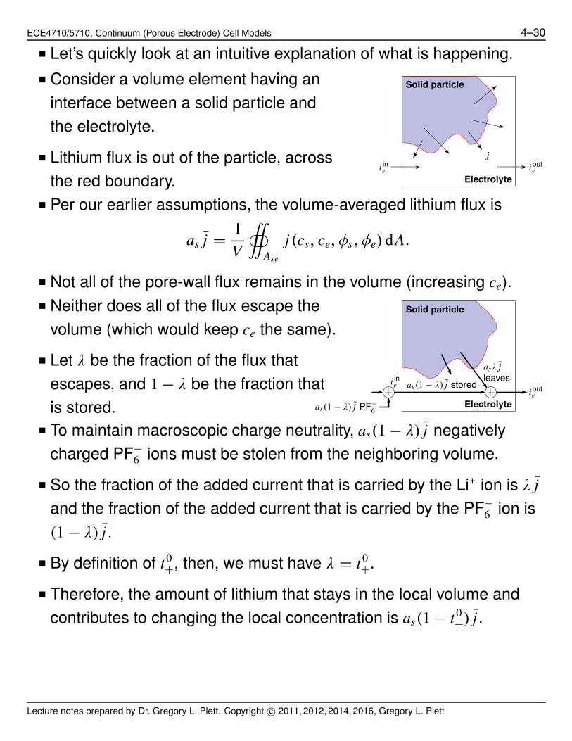
■ Consider a volume element having an
interface between a solid particle and
the electrolyte.
■ Lithium flux is out of the particle, across
the red boundary.
Solid particle
Electrolytei ine iout
e
j
■ Per our earlier assumptions, the volume-averaged lithium flux is
as j =1
V
‹
Ase
j (cs, ce,φs,φe) dA.
■ Not all of the pore-wall flux remains in the volume (increasing ce).
■ Neither does all of the flux escape the
volume (which would keep ce the same).
■ Let λ be the fraction of the flux that
escapes, and 1 − λ be the fraction that
is stored. Electrolyte
Solid particle
i ine
ioute
as(1 − λ) j stored
asλ j
leaves
as(1 − λ) j PF−6
■ To maintain macroscopic charge neutrality, as(1 − λ) j negatively
charged PF−6 ions must be stolen from the neighboring volume.
■ So the fraction of the added current that is carried by the Li+ ion is λ j
and the fraction of the added current that is carried by the PF−6 ion is
(1 − λ) j .
■ By definition of t0+, then, we must have λ = t0
+.
■ Therefore, the amount of lithium that stays in the local volume and
contributes to changing the local concentration is as(1 − t0+) j .
Lecture notes prepared by Dr. Gregory L. Plett. Copyright c⃝ 2011, 2012, 2014, 2016, Gregory L. Plett
ECE4710/5710, Continuum (Porous Electrode) Cell Models 4–31
4.9: Charge conservation in electrolyte; Butler–Volmer; BCs
Charge conservation in electrolyte
■ Recall the microscale electrolyte charge-conservation equation,
∇ · ie = ∇ ·
(
−κ∇φe −2κRT
F
(
1 +∂ ln f±
∂ ln ce
)(
t0+ − 1
)
∇ ln ce
)
= 0.
■ For simplicity, we re-write this as
∇ · ie = ∇ · (−κ∇φe − κD∇ ln ce) = 0,
where we have defined
κD =2κRT
F
(
1 +∂ ln f±
∂ ln ce
)(
t0+ − 1
)
.
■ Using volume-averaging theorem 2 gives
∇ · ie =1
εe
(
∇ ·(
εe ie)
+1
V
‹
Ase
ie · ne dA
)
.
■ We can compute the value of the integral by recalling that
ie · ne = − j F on the interface. Therefore, we approximate the integral
by −as F j .
∇ · ie =1
εe
(
∇ ·(
εe ie)
− as F j)
= 0
0 = ∇ ·(
εeie)
− as F j .
■ Note that
εe ie = εe
(
−κ∇φe + −κD∇ ln ce
)
.
■ As before, we approximate
−εeκ∇φe ≈ −κeff∇φe
−εeκD∇ ln ce ≈ −κD,eff∇ ln ce,
where κeff = κεbruge and κD,eff = κDε
bruge .
Lecture notes prepared by Dr. Gregory L. Plett. Copyright c⃝ 2011, 2012, 2014, 2016, Gregory L. Plett
ECE4710/5710, Continuum (Porous Electrode) Cell Models 4–32
• Mathematically, it might be better to approximate ∇ ln ce ≈ εe∇ ln ce
by doing a Taylor-series expansion of ln ce around ce and keeping
the lower two terms in a volume-average integral.
• This would contribute an extra εe to the result. However this is not
generally done (probably because we can set κD,eff to any value we
want, which might have the extra εe built in already, and probably
because the ln ce term tends not to be as large as the φe term).
■ Combining, we get two results:
εeie = −κeff∇φe − κD,eff∇ ln ce,
and
∇ ·(
κeff∇φe + κD,eff∇ ln ce
)
+ as j F = 0.
Lithium movement between the solid and electrolyte phases
■ We have already used this result, but for completeness we recall that
j = k0c1−αe (cs,max − cs,e)
1−αcαs,e
{
exp
(
(1 − α)F
RTη
)
− exp
(
−αF
RTη
)}
.
■ This shows up in models as:
1
V
‹
Ase
j (cs, ce,φs,φe) dA ≈Ase
Vj (cs,e, ce, φs, φe)
≈ as j (cs,e, ce, φs, φe) = as j .
Boundary conditions for pseudo 2-D model
Charge conservation of the solid
■ The electrical current through the solid at the current collector must
equal the total current entering/exiting the cell. That is,
Lecture notes prepared by Dr. Gregory L. Plett. Copyright c⃝ 2011, 2012, 2014, 2016, Gregory L. Plett
ECE4710/5710, Continuum (Porous Electrode) Cell Models 4–33
εs is = −σeff∇φs =Iapp
A,
where Iapp is the total cell applied current in [A], and A is the
current-collector plate area in [m2].
■ Similarly, the electrical current through the solid at the separator
interface must be zero.
■ For the positive electrode,
∂φs
∂x
∣∣∣∣x=Lneg+Lsep
= 0, and∂φs
∂x
∣∣∣∣
x=L tot
=−Iapp
Aσeff.
■ For the negative electrode,
φs
∣∣x=0
= 0, and∂φs
∂x
∣∣∣∣
x=Lneg
= 0.
■ It is also true, for the anode, that∂φs
∂x
∣∣∣∣
x=0
=−Iapp
Aσeff, but when all PDEs
of the battery model are integrated together, this condition is
redundant and is not implemented.
Mass conservation of the solid
■ Boundary conditions on the mass conservation equation are:
∂cs
∂r
∣∣∣∣r=0
= 0, and Ds
∂cs
∂r
∣∣∣∣r=Rs
= − j ,
where positive j indicates lithium flowing out of the particle.
Mass conservation of the electrolyte
■ There must be no electrolyte flux at the cell boundaries
∂ ce
∂x
∣∣∣∣
x=0
=∂ ce
∂x
∣∣∣∣
x=L tot
= 0.
Lecture notes prepared by Dr. Gregory L. Plett. Copyright c⃝ 2011, 2012, 2014, 2016, Gregory L. Plett
ECE4710/5710, Continuum (Porous Electrode) Cell Models 4–34
Charge conservation of the electrolyte
■ The ionic current must be zero at the current collectors. At the
separator boundaries, the ionic current must equal the total current
entering/exiting the cell:
εeie = −κeff∇φe − κD,eff∇ ln ce =Iapp
A.
■ So, at the current collector boundaries, we have:
κeff∂φe
∂x+ κD,eff
∂ ln ce
∂x
∣∣∣∣x=0
= κeff∂φe
∂x+ κD,eff
∂ ln ce
∂x
∣∣∣∣x=L tot
= 0.
■ As before, we have boundary conditions at the separator interfaces,
but these are redundant and not implemented:
−κeff∂φe
∂x− κD,eff
∂ ln ce
∂x
∣∣∣∣
x=Lneg
= −κeff∂φe
∂x− κD,eff
∂ ln ce
∂x
∣∣∣∣
x=Lneg+Lsep
=Iapp
A.
Lecture notes prepared by Dr. Gregory L. Plett. Copyright c⃝ 2011, 2012, 2014, 2016, Gregory L. Plett
ECE4710/5710, Continuum (Porous Electrode) Cell Models 4–35
4.10: Cell-level quantities; PDE simulation methods
Cell voltage
■ Cell voltage is equal to the positive current-collector’s potential minus
the negative current-collector’s potential.
■ Since the solid phase is in direct electrical contact with the current
collector, we then compute the cell voltage as
v(t) = φs(L tot, t) − φs(0, t).
■ And, since we have defined φs(0, t) = 0, we can further simplify to
v(t) = φs(L tot, t).
Cell total capacity
■ Cell total capacity is determined in the same manner as in Chap. 3:
Qneg = AF Lnegεnegs cneg
s,max |x100% − x0%| /3600Ah
Qpos = AF Lposεposs cpos
s,max |y100% − y0%| /3600Ah,
and
Q = min(
Qneg, Qpos)
Ah.
Cell state of charge
■ Similarly, cell state of charge is determined in the same manner as in
Chap. 3:
z =c
negs,avg/c
negs,max − x0%
x100% − x0%
=c
poss,avg/c
poss,max − y0%
y100% − y0%
.
Lecture notes prepared by Dr. Gregory L. Plett. Copyright c⃝ 2011, 2012, 2014, 2016, Gregory L. Plett
ECE4710/5710, Continuum (Porous Electrode) Cell Models 4–36
Model simulations
■ We have the full set of equations for the continuous scale, which is
great, but useless unless we can do something with them.
■ One very important application of the model is to use it in simulation
to help understand how a cell works, and then use that to inform how
a cell should be built, and/or how a cell should be operated.
■ Digital simulation of continuous phenomena require discretizing the
problem in time and space.
FINITE DIFFERENCE: Divide space and time into small segments.
■ Discretize the derivatives in the equations using Euler’s rule or
similar over these segments.
■ Write the resulting system of equations, and solve using a linear
algebra solver at each time step.
■ The linear diffusion example in Chap. 3 introduced this method.
FINITE VOLUME: Divide time into small segments, space into volumes.
■ Flux terms at volume boundaries are evaluated, and
concentrations are updated to reflect the material fluxes.
■ This method enforces mass balance: because the flux entering a
given volume is identical to that leaving the adjacent volume, these
methods are conservative.
■ Another advantage of the finite volume method is that it is easily
formulated to allow for unstructured meshes.
■ The method is used in many CFD packages.
■ The spherical diffusion example in Chap. 3 introduced this method.
Lecture notes prepared by Dr. Gregory L. Plett. Copyright c⃝ 2011, 2012, 2014, 2016, Gregory L. Plett
ECE4710/5710, Continuum (Porous Electrode) Cell Models 4–37
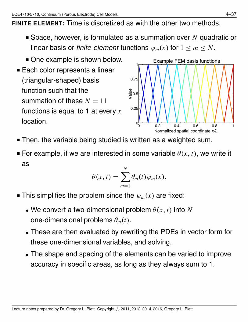
FINITE ELEMENT: Time is discretized as with the other two methods.
■ Space, however, is formulated as a summation over N quadratic or
linear basis or finite-element functions ψm(x) for 1 ≤ m ≤ N .
■ One example is shown below.
■ Each color represents a linear
(triangular-shaped) basis
function such that the
summation of these N = 11
functions is equal to 1 at every x
location.0 0.2 0.4 0.6 0.8 10
0.25
0.5
0.75
1Example FEM basis functions
Normalized spatial coordinate x/LVa
lue
■ Then, the variable being studied is written as a weighted sum.
■ For example, if we are interested in some variable θ(x, t), we write it
as
θ(x, t) =
N∑
m=1
θm(t)ψm(x).
■ This simplifies the problem since the ψm(x) are fixed:
• We convert a two-dimensional problem θ(x, t) into N
one-dimensional problems θm(t).
• These are then evaluated by rewriting the PDEs in vector form for
these one-dimensional variables, and solving.
• The shape and spacing of the elements can be varied to improve
accuracy in specific areas, as long as they always sum to 1.
Lecture notes prepared by Dr. Gregory L. Plett. Copyright c⃝ 2011, 2012, 2014, 2016, Gregory L. Plett
ECE4710/5710, Continuum (Porous Electrode) Cell Models 4–38
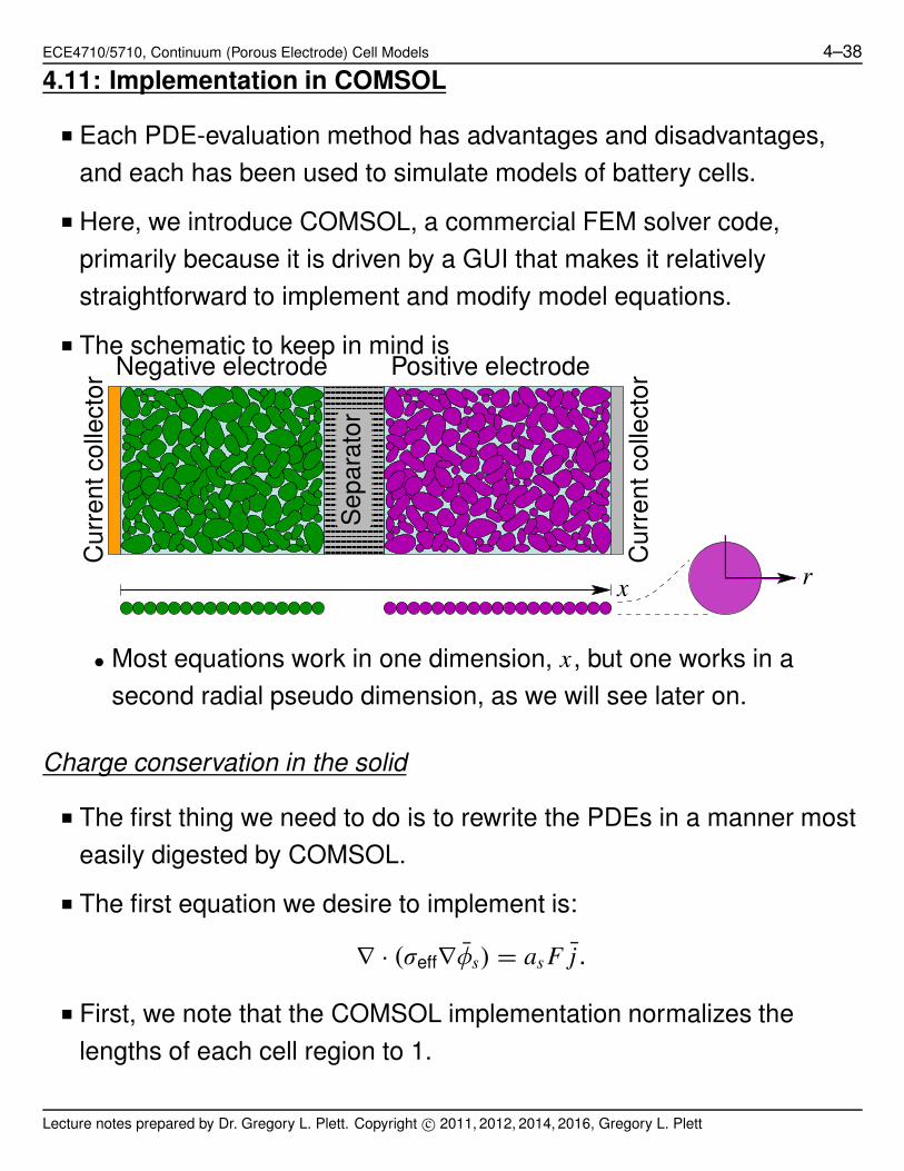
4.11: Implementation in COMSOL
■ Each PDE-evaluation method has advantages and disadvantages,
and each has been used to simulate models of battery cells.
■ Here, we introduce COMSOL, a commercial FEM solver code,
primarily because it is driven by a GUI that makes it relatively
straightforward to implement and modify model equations.
■ The schematic to keep in mind isNegative electrode Positive electrode
Cu
rre
ntco
llect
or
Cu
rre
ntco
llect
or
Se
pa
rato
r
x r
• Most equations work in one dimension, x , but one works in a
second radial pseudo dimension, as we will see later on.
Charge conservation in the solid
■ The first thing we need to do is to rewrite the PDEs in a manner most
easily digested by COMSOL.
■ The first equation we desire to implement is:
∇ · (σeff∇φs) = as F j .
■ First, we note that the COMSOL implementation normalizes the
lengths of each cell region to 1.
Lecture notes prepared by Dr. Gregory L. Plett. Copyright c⃝ 2011, 2012, 2014, 2016, Gregory L. Plett
ECE4710/5710, Continuum (Porous Electrode) Cell Models 4–39
■ We will use symbol x to represent position with respect to normalized
length, and x to denote actual position.
■ In the negative electrode, x = x/Lneg; in the positive electrode,
x = (x − Lneg − Lsep)/Lpos. Generically x = x/L + cst.
■ Therefore, also,∂(·)
∂ x=∂(·)
∂x
∂x
∂ x= L
∂(·)
∂x
∂(·)
∂x=∂(·)
∂ x
∂ x
∂x=
1
L
∂(·)
∂ x.
■ This changes the equation we wish to implement to:
1
L∇ ·
(σeff
L∇φs
)
= as F j .
■ The COMSOL implementation multiplies both sides by L (better
convergence)
∇ · (sigma_eff/L ∗ phi_sx) = L ∗ as ∗ F ∗ j,
where the following variables are defined
σeff as j L φs F
sigma_eff as j L phi_s F
■ Note that in COMSOL syntax,
phi_sx =d
dxphi_s,
and COMSOL’s “x” is our normalized dimension “x”.
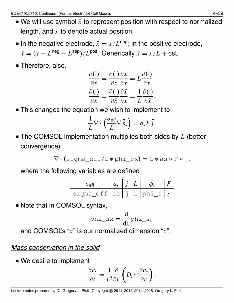
Mass conservation in the solid
■ We desire to implement
∂cs
∂t=
1
r2
∂
∂r
(
Dsr2∂cs
∂r
)
.
Lecture notes prepared by Dr. Gregory L. Plett. Copyright c⃝ 2011, 2012, 2014, 2016, Gregory L. Plett
ECE4710/5710, Continuum (Porous Electrode) Cell Models 4–40
■ Note that this equation operates in the “pseudo” dimension, r , instead
of the linear dimension x .
■ That is, at every “x” location, a copy of this radial equation is
operating, representing the radially symmetric concentration profile of
lithium in a representative spherical particle sitting at that “x” location.
■ We also normalize the radial dimension: Let r = r/Rs.
■ Then, r2 = R2s r2 and
∂(·)
∂r=
1
Rs
∂(·)
∂r. This allows us to re-write our PDE
as∂cs
∂t=
(
1
R2s r2
)
1
Rs
∂
∂r
(
Ds
(
R2s r2
) 1
Rs
∂cs
∂r
)
.
■ Multiply both sides of the equation by r2 Rs and rearrange to get what
COMSOL implements
r2 Rs
∂
∂tcs +
∂
∂r
(
−Ds
r2
Rs
∂cs
∂r
)
= 0,
except that COMSOL uses y instead of r .
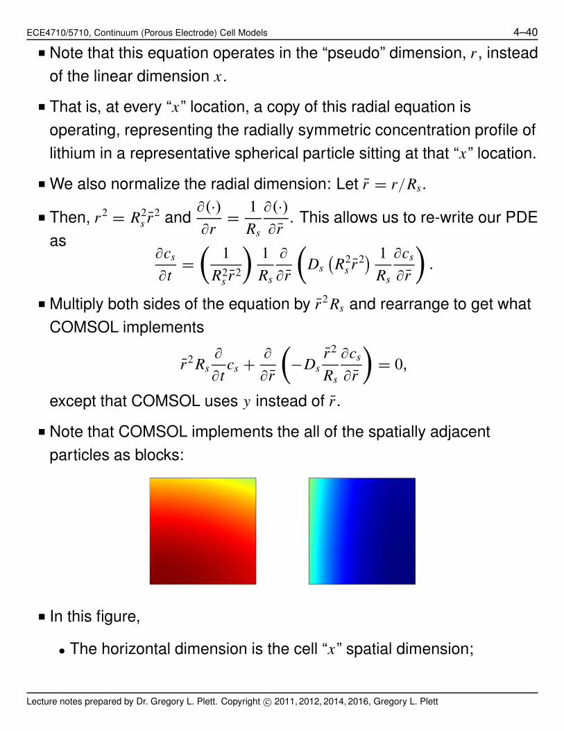
■ Note that COMSOL implements the all of the spatially adjacent
particles as blocks:
■ In this figure,
• The horizontal dimension is the cell “x” spatial dimension;
Lecture notes prepared by Dr. Gregory L. Plett. Copyright c⃝ 2011, 2012, 2014, 2016, Gregory L. Plett
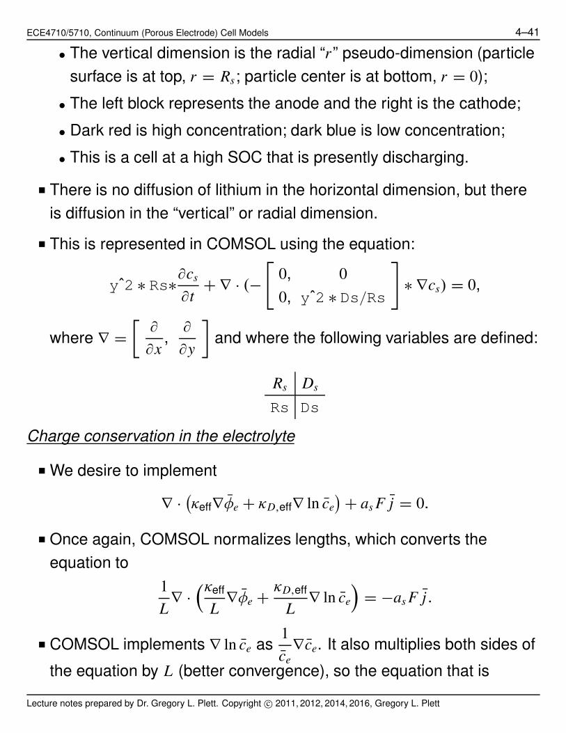
ECE4710/5710, Continuum (Porous Electrode) Cell Models 4–41
• The vertical dimension is the radial “r” pseudo-dimension (particle
surface is at top, r = Rs; particle center is at bottom, r = 0);
• The left block represents the anode and the right is the cathode;
• Dark red is high concentration; dark blue is low concentration;
• This is a cell at a high SOC that is presently discharging.
■ There is no diffusion of lithium in the horizontal dimension, but there
is diffusion in the “vertical” or radial dimension.
■ This is represented in COMSOL using the equation:
yˆ2 ∗ Rs∗∂cs
∂t+ ∇ · (−
[
0, 0
0, yˆ2 ∗ Ds/Rs
]
∗ ∇cs) = 0,
where ∇ =
[
∂
∂x,∂
∂y
]
and where the following variables are defined:
Rs Ds
Rs Ds
Charge conservation in the electrolyte
■ We desire to implement
∇ ·(
κeff∇φe + κD,eff∇ ln ce
)
+ as F j = 0.
■ Once again, COMSOL normalizes lengths, which converts the
equation to
1
L∇ ·
(κeff
L∇φe +
κD,eff
L∇ ln ce
)
= −as F j .
■ COMSOL implements ∇ ln ce as1
ce
∇ ce. It also multiplies both sides of
the equation by L (better convergence), so the equation that is
Lecture notes prepared by Dr. Gregory L. Plett. Copyright c⃝ 2011, 2012, 2014, 2016, Gregory L. Plett
ECE4710/5710, Continuum (Porous Electrode) Cell Models 4–42
actually implemented is:
∇ · (kappa_eff/L ∗ (phi_ex+ kappa_D_fact ∗ 1/c_e ∗ c_ex))
= −L ∗ as ∗ F ∗ j.
where the following variables are defined
κeff κD,eff/κeff as j L φe ce F
kappa_eff kappa_D_fact as j L phi_e c_e F
■ Note again that in COMSOL syntax,
phi_ex =d
dxphi_e and c_ex =
d
dxc_e,
and COMSOL’s “x” is our normalized dimension “x”.
Mass conservation in the electrolyte
■ We desire to implement
∂(εece)
∂t= ∇ · (De,eff∇ ce) + as(1 − t0
+) j .
■ Once again, COMSOL normalizes lengths, which converts the
equation to
∂(εece)
∂t=
1
L∇ · (De,eff
1
L∇ ce) + as(1 − t0
+) j .
■ What is actually implemented is
eps_e ∗ L ∗∂ce
∂t+ ∇ · (−De_eff/L ∗ ∇ce) = L ∗ as ∗ (1 − t_plus) ∗ j,
where the following variables are defined
De,eff t0+ as j L εe
De_eff t_plus as j L eps_e
Lecture notes prepared by Dr. Gregory L. Plett. Copyright c⃝ 2011, 2012, 2014, 2016, Gregory L. Plett
ECE4710/5710, Continuum (Porous Electrode) Cell Models 4–43
Butler–Volmer equation
■ Notice that the units of k0 are rather awkward.
• The exponential terms of the Butler–Volmer equation are unitless,
and j has units mol m−2 s−1.
• Therefore, k0 must have units of molα−1 m4−3α s−1.
• COMSOL struggles with units having non-integer powers, so this
poses a problem.
■ A solution is to define a normalized exchange current density
i0 = Fk0c1−αe (cs,max − cs,e)
1−αcαs,e
= F k0c1−αe,0 cs,max
︸ ︷︷ ︸
knorm0
(
ce
ce,0
)1−α (
cs,max − cs,e
cs,max
)1−α (
cs,e
cs,max
)α
,
where ce,0 is the at-rest concentration of lithium in the electrolyte.
■ Re-arranging the exchange current density in this form makes the
terms raised to non-integer powers themselves unitless, and gives
knorm0 units of mol m−2 s−1, which is much easier to work with.
■ We can rewrite the Butler–Volmer equation as
j = knorm0
((
ce
ce,0
) (
cs,max − cs,e
cs,max
))1−α (
cs,e
cs,max
)α
×
{
exp
(
(1 − α)F
RTη
)
− exp
(
−αF
RTη
)}
.
■ Also note: most articles that discuss simulation of lithium-ion cells do
not give values for k0. Instead, they give values of i0 that apply at the
beginning of the simulation, from which you must derive k0 or knorm0 .
Lecture notes prepared by Dr. Gregory L. Plett. Copyright c⃝ 2011, 2012, 2014, 2016, Gregory L. Plett
ECE4710/5710, Continuum (Porous Electrode) Cell Models 4–44
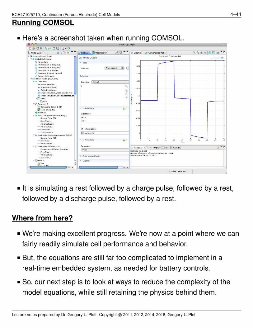
Running COMSOL
■ Here’s a screenshot taken when running COMSOL.
■ It is simulating a rest followed by a charge pulse, followed by a rest,
followed by a discharge pulse, followed by a rest.
Where from here?
■ We’re making excellent progress. We’re now at a point where we can
fairly readily simulate cell performance and behavior.
■ But, the equations are still far too complicated to implement in a
real-time embedded system, as needed for battery controls.
■ So, our next step is to look at ways to reduce the complexity of the
model equations, while still retaining the physics behind them.
Lecture notes prepared by Dr. Gregory L. Plett. Copyright c⃝ 2011, 2012, 2014, 2016, Gregory L. Plett
ECE4710/5710, Continuum (Porous Electrode) Cell Models 4–45
Glossary
■ as(x, y, z, t) [m2 m−3] is the specific interfacial area: the area of the
boundary between solid and electrolyte per unit volume.
■ ce(x, y, z, t) [mol m−3] is the intrinsic volume average concentration of
lithium in the electrolyte in the vicinity of a particular location.
■ cs,e(x, y, z, t) [mol m−3] is the intrinsic volume average concentration
of lithium at the interface between solid and electrolyte in the vicinity
of a particular location.
■ δ(x, y, z, t) [unitless] is the constrictivity of a porous media in the
vicinity of a point. δ < 1.
■ De,eff(x, y, z, t) [m2 s−1] is a short form for De,eff ≈ Deεbruge = Deε
1.5e .
■ εe(x, y, z, t) [unitless] is the porosity or volume fraction of the
electrolyte phase in an electrode (other phases include the solid
phase and inert-materials phase).
■ εs(x, y, z, t) [unitless] is the volume fraction of the solid phase in an
electrode (other phases include the electrolyte phase and
inert-materials phase).
■ φ(x, y, z, t) [V] is the scalar field representing the electric potential at
a given point.
■ φe(x, y, z, t) [V] is the intrinsic volume averaged scalar field
representing the electric potential in the electrolyte in the vicinity of a
given point.
■ φs(x, y, z, t) [V] is the intrinsic volume averaged scalar field
representing the electric potential in the solid in the vicinity of a given
point.
Lecture notes prepared by Dr. Gregory L. Plett. Copyright c⃝ 2011, 2012, 2014, 2016, Gregory L. Plett
ECE4710/5710, Continuum (Porous Electrode) Cell Models 4–46
■ j (x, y, z, t) [mol m−2 s−1] is the rate of positive charge flowing out of a
particle across a boundary between the solid and the electrolyte.
■ j(x, y, z, t) [mol m−2 s−1] is the volume-averaged rate of positive
charge flowing out of a particle across a boundary between the solid
and the electrolyte.
■ κ(x, y, z, t) [S m−1] is a material-dependent parameter of the
electrolyte called the bulk conductivity of homogenous materials
without inclusions in the vicinity of a given point.
■ κeff(x, y, z, t) [S m−1] is the effective conductivity of the electrolyte,
representing a volume averaged conductivity of the electrolyte phase
in a porous media in the vicinity of a given point. We often model
κeff ≈ κεbruge = κε1.5
e .
■ κD,eff(x, y, z, t) [A m−1] is a short form for κD,eff ≈ κDεbruge = κDε
1.5e .
■ σ (x, y, z, t) [S m−1] is a material-dependent parameter of the solid
electrode particles called the bulk conductivity of homogenous
materials without inclusions in the vicinity of a given point.
■ σeff(x, y, z, t) [S m−1] is an electrode-dependent parameter called the
effective conductivity, representing a volume averaged conductivity of
the solid matrix in a porous media in the vicinity of a given point. We
often model σeff ≈ σεbrugs = σε1.5
s .
■ τ (x, y, z, t) [unitless] is the tortuosity of the porous media in the
vicinity of a point. τ ≥ 1.
Lecture notes prepared by Dr. Gregory L. Plett. Copyright c⃝ 2011, 2012, 2014, 2016, Gregory L. Plett