continuous basalt fiber as reinforcement material in ... n-ólafur... · pdf filei...
TRANSCRIPT
i
Continuous Basalt Fiber as Reinforcement Material in Polyester Resin
by
Jón Ólafur Erlendsson
Master of Science in Civil Engineering with
Specialization in Structural Design
August 2012
ii
Continuous Basalt Fiber as Reinforcement Material in Polyester Resin
Jón Ólafur Erlendsson
Thesis (30 ECTS) submitted to the School of Science and Engineering
at Reykjavík University in partial fulfillment of the requirements for the degree of
Master of Science in Civil Engineering with Specialization in Structural Design
August 2012
Supervisor:
Eyþór Rafn Þórhallsson Associate Professor, Reykjavík University, Iceland
Examiner:
Dr. Sigurður Brynjólfsson Associate Professor, University of Iceland
i
Abstract
The industry is always striving to find new and better materials to manufacture new or
improved products. Within this context, energy conservation, corrosion, sustainability
and other environmental issues are important factors in product development. Basalt
fibers are a natural material, produced from igneous rock which can provide high
strength relative to weight. Research has also shown that basalt fibers have many
other advantageous qualities.
This thesis describes an applied research project, investigating the material
characteristics of a relatively new material, continuous basalt fibers in polyester resin.
The objective was to examine whether a composite material made of polyester resin
reinforced with basalt fibers, could be used for engineering structures. The project
combines two phases. The first phase was a basic research of material properties
where specimens made of basalt fibers in polyester resin were constructed and tested
according to the ASTM standard. The second phase was the construction and testing
of two1200 mm long tubes made of basalt fiber in polyester resin.
The material testing phase included a study of simple state of the art methods used to
analyze layered composite materials layer (laminate) by layer. Various standard load
tests were then applied to the samples. A uniaxial static tensile test, a uniaxial
compression test, an in-plane shear test and a pin bearing test were carried out. The
test results were compared with published test results for similar composite materials,
such as glass fibers in epoxy and carbon fibers in epoxy.
The results of the material testing indicated that basalt fibers can be used as
reinforcement material in polyester resin, to create a composite structural material
with acceptable engineering properties. The comparison with other similar results for
other composite materials showed that basalt fibers in polyester resin were in fact
19.3% stronger in tension than glass fibers in epoxy resin.
Structural testing of the 1200 mm long tube, built using a composite material of basalt
fiber reinforced polyester resin revealed, that the tube was strong enough to meet the
standard design criteria’s specified for a regular four-meter high lamppost.
Keywords: Basalt fiber, basalt fabric, continuous basalt fibers, polyester resin, composite material, laminate material, structural testing.
ii
Ágrip - Basaltþræðir sem styrkingarefni í polyester plastefni
Iðnaðurinn er stöðugt að leitast við að finna ný og betri efni til að framleiða nýjar og/eða endurbættar vörur. Orkusparnaður, tæringarhætta, sjálfbærni og aðrir umhverfisþættir hafa mikil áhrif á val á nýjum efnum og tilsvarandi vöruþróun.
Í þessari ritgerð er kynnt hagnýtt rannsóknarverkefni þar sem nýtt efni, polyester plastefni styrkt með basaltþráðum var prófað til að athuga hæfni þess til notkunar í mannvirkjagerð. Basalt trefjar er náttúrulegt efni sem unnið er úr storkuberginu basalt sem getur gefið mikinn styrk í hlutfalli af eiginþyngd. Einnig hefur komið fram í rannsóknum að basalt trefjar hafa marga aðra hagnýta efniseiginleika.
Verkefnið var tvíþætt. Meginmarkmið verkefnisins var að rannsaka hvort hægt væri að nota basaltþræði, sem styrkingarefni í polyester plastefni til að búa til samsett efni með eiginleika sem henta til mannvirkjagerðar. Þessi rannsókn flokkast undir grunnrannsókn í efnisfræði trefjaefna þar sem prófaðir voru efnisbútar, gerðir úr basaltþráðum í polyester fylliefni, í samræmi við viðurkenndan alþjóðlegan staðal (ASTM). Einnig voru búnir til tveir staurar, 1200 mm langir, úr basaltþráðum í polyester fylliefni. Annar staurinn var innspenntur í annan endann og burðarþolsprófaður með því að setja stakan kraft á hinn endann með stefnu þvert á langstefnu bitans. Hinn staurinn var steyptur niður í fjörunni í Keflavík til að langtíma prófunar á áhrifum veðrunar og annarra umhverfisþátta.
Til að kanna brotstyrk samsetta trefjaefnisins voru gerð mismunandi einása, stöðufræðileg álagspróf. Um var að ræða togþolspróf, þrýstiþolspróf, skerþolspróf og prófun á boltaðri skúftengingu. Niðurstöðurnar voru bornar saman innbyrðis milli einstakra sýna sem og við birtar rannsóknarniðurstöður fyrir önnur sambærileg efni eins og glertrefja- og koltrefjastyrkt epoxy efni. Í tengslum við ofangreindar prófanir voru hefðbundnar reikniaðferðir til greiningar á brotþoli lagskiptra efna kannaðar. Niðurstöður rannsóknarinnar á burðargetu efnissýna, gáfu til kynna að hægt er að búa til samsett efni úr basaltþráðum og polyester fylliefni sem hefur nothæfa verkfræðilega eiginleika. Samanburður á niðurstöðum við aðrar rannsóknir leiddi einnig í ljós að samsett efni úr basalttrefjastyrktu polyester gaf 19.3% meiri styrk í togi heldur en samsett efni úr glertrefjastyrktu epoxy. Álagsprófun innspenntrar súlu úr basalttrefjastyrktu polyester leiddi í ljós að staurinn uppfyllir hefðbundnar hönnunarkröfur fyrir fjögurra metra háan ljósastaur. Lykilorð: Basalttrefjar, basalt mottur, basaltþræðir, polyester plastefni, samsett efni, lagskipt efni, trefjaplast, burðarþolsprófanir.
iv
Acknowledgements
First of all I want to thank my lovely family for their grateful support and being
patient for the past five years, through my entire B.Sc. and M.Sc. study. Without their
support this study would not have been feasible.
I thank my supervisor Eyþór Rafn Þórhallsson, civil engineer, M.Sc. and associate
professor at Reykjavik University, for coming up with this applied project. I wish also
to thank him for his guidance and inspiration throughout the entire project.
Special thanks go to all the good people and companies who helped me with the
experimental work. Andri Thor Gunnarsson, general manager at Infuse, for
manufacturing the plates with the Vacuum Infusion process. Trésmiðja Ella Jóns, for
the facilities to cut the specimens and create the tubes. Innovation Center Iceland for
the facilities to perform the experiment (part 1). Hreinn Jónsson at Innovation Center
Iceland for assistance in the experiment (part 1).
Finally I want to thank the staff at Reykjavik University: Gísli Þorsteinsson,
technician; Indriði Ríkharðsson, mechanical engineer, M.Sc.; and Hrannar Traustason,
electronics engineer, for assistance in the experimental work.
v
Table of Contents ABSTRACT .................................................................................................................. I
ÁGRIP - BASALTÞRÆÐIR SEM STYRKINGAREFNI Í POLYESTER PLASTEFNI ................................................................................................................ II
ACKNOWLEDGEMENTS ..................................................................................... IV
TABLE OF CONTENTS ........................................................................................... V
LIST OF FIGURES ............................................................................................... VIII
LIST OF TABLES ................................................................................................. XIV
NOTATION .............................................................................................................. XV
ABBREVIATIONS ............................................................................................... XVII
INTRODUCTION ........................................................................................................ 1
1.1 GENERAL .............................................................................................................. 1 1.2 PROBLEM OVERVIEW ............................................................................................ 1 1.3 OVERVIEW OF WORK ON BASALT FIBERS ............................................................... 4 1.4 OBJECTIVES........................................................................................................... 4 1.5 THESIS OVERVIEW ................................................................................................ 5
BACKGROUND .......................................................................................................... 6
2.1 GENERAL .............................................................................................................. 6 2.2 COMPOSITE MATERIAL .......................................................................................... 6
2.2.1 Resin Systems ............................................................................................... 6 2.2.2 Reinforcements (fiber) .................................................................................. 7 2.2.3 Manufacturing Processes for laminate material ............................................ 7
2.3 ANALYTICAL MODELING (ANALYSIS OF COMPOSITE MATERIALS) ......................... 9 2.3.1 Micromechanics of a unidirectional ply ..................................................... 10 2.3.2 Classical Laminate Theory ......................................................................... 16 2.3.3 Failure theories ............................................................................................ 20 2.3.4 Laminate Design Software .......................................................................... 24
2.4 TEST METHODS ................................................................................................... 24 2.5 SUMMARY ........................................................................................................... 25
MATERIAL PROPERTIES IN THE EXPERIMENT .......................................... 26
3.1 GENERAL ............................................................................................................ 26 3.2 BASALT FIBER ..................................................................................................... 26 3.3 POLYESTER RESIN ............................................................................................... 27 3.4 SUMMARY ........................................................................................................... 27
EXPERIMENTAL PROGRAM AND PROCEDURES, PART 1 ......................... 28
4.1 GENERAL ............................................................................................................ 28 4.2 FABRICATION PROCEDURE OF THE FIBER PLATES................................................ 28 4.2 CONSTITUENT CONTENT DETERMINATION OF THE FIBER PLATES ....................... 29 4.3 TENSILE TEST PROCEDURE ................................................................................. 31
4.3.1 Fabrication Procedure of Specimens A and C ............................................ 31 4.3.2 Test Procedure of Specimens A and C ....................................................... 32
4.4 COMPRESSION TEST PROCEDURE ........................................................................ 34 4.4.1 Fabrication Procedure of Specimens D and E ............................................ 34
vi
4.4.2 Test Procedure of Specimens D and E ........................................................ 35 4.5 IN-PLANE SHEAR TEST ± 45° PROCEDURE .......................................................... 38
4.5.1 Fabrication Procedure of Specimens B ....................................................... 38 4.5.2 Test Procedure of Specimens B .................................................................. 39
4.6 PIN BEARING TEST PROCEDURE .......................................................................... 40 4.6.1 Fabrication Procedure of Specimens G, H and I ......................................... 40 4.6.2 Test Procedure of Specimens G, H and I .................................................... 41
4.7 SUMMARY ........................................................................................................... 43
EXPERIMENTAL PROGRAM AND PROCEDURES, PART 2 ......................... 44
5.1 GENERAL ............................................................................................................ 44 5.2 FABRICATION PROCEDURE OF THE TUBES ........................................................... 44 5.3 CONSTITUENT CONTENT DETERMINATION OF THE TUBES ................................... 45 5.4 WEATHERING TEST OF THE TUBE ........................................................................ 46 5.5 LOAD TEST PROCEDURE OF THE TUBE ................................................................ 47 5.6 SUMMARY ........................................................................................................... 48
EXPERIMENTAL RESULTS .................................................................................. 49
6.1 GENERAL ............................................................................................................ 49 6.2 CONSTITUENT CONTENT DETERMINATION RESULTS ........................................... 49 6.3 TENSILE TEST RESULTS ...................................................................................... 50
6.3.1 General Behavior and Mode Failure of Specimens A and C ...................... 50 6.3.2 Test Results of Specimens A and C ............................................................ 53
6.4 COMPRESSION TEST RESULTS ............................................................................. 57 6.4.1 General Behavior and Mode Failure of Specimens D and E ...................... 57 6.4.2 Test Results of Specimens D and E ............................................................ 60
6.5 IN-PLANE SHEAR TEST ± 45° RESULTS ............................................................... 62 6.5.1 General Behavior and Mode Failure of Specimens B ................................ 62 6.5.2 Test Results of Specimens B ....................................................................... 63
6.6 PIN BEARING STRENGTH TEST ............................................................................ 65 6.6.1 General Behavior and Mode Failure of Specimens G, H and I .................. 65 6.6.2 Test Results of Specimens G, H and I ........................................................ 68
6.7 TUBE TEST RESULTS ........................................................................................... 72 6.7.1 Weathering Test Results of Tube no.1 ........................................................ 72 6.7.2 Load Test Results of Tube no.2 .................................................................. 72
6.8 SUMMARY ........................................................................................................... 73
DISCUSSION ............................................................................................................. 74
7.1 GENERAL ............................................................................................................ 74 7.2 CONCLUSION OF RESEARCH ................................................................................ 74
7.2.1 Constituent Content Determination Conclusion ......................................... 74 7.2.2 Tensile Test Conclusion of Specimens A and C ......................................... 74 7.2.3 Compression Test Conclusion of Specimens D and E ................................ 75 7.2.3 In-Plane Shear Test ± 45° Conclusion of Specimens B .............................. 75 7.2.3 Pin Bearing Strength Test Conclusion of Specimens G, H and I ............... 75
7.3 CALCULATED ACCORDING TO CLT AND THE FAILURE THEORIES ....................... 76 7.4 COMPARISON WITH OTHER COMPOSITE MATERIALS ........................................... 82 7.5 CONCLUSION OF THE TUBE RESEARCH ................................................................ 84
7.5.1 Load Test Comparison of Tube no.2 .......................................................... 84 7.5.2 Load Test Conclusion of Tube no.2 ............................................................ 84
vii
7.6 SUMMARY ........................................................................................................... 85
SUMMARY ................................................................................................................ 86
8.1 GENERAL ............................................................................................................ 86 8.2 FURTHER RESEARCH ........................................................................................... 86
REFERENCES ........................................................................................................... 87
APPENDIX A – TECHNICAL DATA OF BASALT FABRICS .......................... 91
APPENDIX B – TECHNICAL DATA OF POLYESTER RESINS ..................... 93
APPENDIX C–MEASURED VALUES ................................................................... 97
APPENDIX D – ORIGINAL GRAPHS ................................................................. 101
APPENDIX E – FAILURE MODELS ................................................................... 108
APPENDIX F – MATLAB CODE ......................................................................... 111
APPENDIX G – VIDEOS OF THE EXPERIMENTS (DVD) ............................. 119
viii
List of figures
Figure 1-1 Transmission poles made of glass fiber in polymer matrix (“Shakespeare
composite structures,” n.d.)…………………………………….………….…………..2
Figure 1-2 Bridge’s carriageway made of glass fiber in polymer matrix (“Europe’s
first plastic bridge is open,” 2010)…………………………………………………….3
Figure 1-3 Swedish warships, 72 m long, made of carbon fiber in polymer matrix
(McGeorge, D. & Höyning, B., n.d.)…………………………………………………..3
Figure 1-4 Airplane, 787 Dreamliner, made of carbon and glass fiber in polymer
matrix (Boeing, n.d.)…………………………………………………………………..4
Figure 2-1 Properties for FRP with combine of the properties from the resin and
fibre (SP Systems, n.d.)………………………………………………………………..6
Figure 2-2 Hand Lay-up manufacturing processes for laminate material (SP Systems,
n.d., p. 51)……………………………………………………………………………...8
Figure 2-3 Vacuum Bagging manufacturing processes for laminate material (SP
Systems, n.d., p. 53)…………………………………………………………………...8
Figure 2-4 Vacuum Infusion manufacturing processes for laminate material (SP
Systems, n.d., p. 57)…………………………………………………………….……..8
Figure 2-5 Three steps to design and analyze composite materials (Meunier, M. &
Knibbs, S., 2007)………………………………………………………………………9
Figure 2-6 Section cut from a fiber-reinforced composite material and a unit cell
(Hyer, 2008, p. 141)………………………………………………………………….10
Figure 2-7 Rule-of-mixtures model for composite modulus of elasticity E1 and
Poisson’s ratio ν12 (Hyer, 2008, p. 142)……………………………………………...11
Figure 2-8 Rule-of-mixtures model for composite modulus of elasticity E2 (Hyer,
2008, p. 146)…………………………………………………………………….……12
Figure 2-9 Rule-of-mixtures model for composite shear modulus of elasticity G12
(Hyer, 2008, p. 154)…………………...……………………………………….…….12
ix
Figure 2-10 Six stress components acting on the element surfaces (Hyer, 2008, p.
46)…………………………………………………………………………………….13
Figure 2-11 Three stress components acting on the composite material element
surfaces in the 1-2 plane (Hyer, 2008, p. 166)……………………………………….14
Figure 2-12 x-y axes are global coordinate system, 1-2 axes are local coordinate
system and θ is the angle between these two coordinate systems (Jones, 1998, p.
75)…………………………………………………………………………………….15
Figure 2-13 The model setup for the z-axis in the Classical Laminate theory (Jones,
1998, p. 196)………………………………………………………………………….16
Figure 2-14 Consequences of Kirchhoff hypothesis, geometry of deformation in the
x-y plane (Jones, 1998, p. 193)………………………………………………………17
Figure 2-15 In plane forces and moments on a flat laminate (Jones, 1998, p.
196)…………………………………………………………………………………...19
Figure 2-16 Comparison between maximum stress theory, maximum strain theory
and interactive failure theories (“Failure Theories,” n.d.)……………………………23
Figure 3-1 Basalt fabrics from Basaltex, the left side is BAS BI 600 and the right
side is BAS UNI 600…………………………………………………………………26
Figure 4-1 Basalt fabrics type BAS BI 600 (to the left) and vacuum infusion process
(to the right)…………………………………………………………………………..28
Figure 4-2 The polyester resin was infused through the basalt fabrics (to the left).
The laminate plates completed after the vacuum infusion process (to the right)…….29
Figure 4-3 Dimensions of the tensile specimen, types A and C………………….....31
Figure 4-4 Six specimens of type A ready to be tensile tested (to the left) and six
specimens of type C ready to be tensile tested (to the right)…………………………31
Figure 4-5 To the left is the computer which collected data from the strain gages, in
the middle is the Tinius Olsen universal testing machine and to the right the computer
which collected data from the Tinius Olsen universal testing machine……………...32
x
Figure 4-6 Tensile test performed on specimen C-04………………………………33
Figure 4-7 Dimensions of the compressive specimen with the gage length 13 m….34
Figure 4-8 The aluminum duct with the specimens inside (to the left) and specimens
of types D and E ready to be compression tested (to the right)………………………35
Figure 4-9 Tinius Olsen machine which was used in the compression tests……….35
Figure 4-10 Compression test performed on specimen D-04……………………….36
Figure 4-11 Tinius Olsen Video Extensometers set up in the compression test……37
Figure 4-12 Dimension of the in-plane shear specimen type B……….……..……..38
Figure 4-13 Six specimens of type B before the strain gages were put on………....38
Figure 4-14 In-plane shear test performed on specimen B-05………………...……39
Figure 4-15 Dimensions of the pin bearing specimen types G, H and I……………40
Figure 4-16 The specimens in types G, H and I with the steel fixture……………..41
Figure 4-17 Tinius Olsen machine which was used in the pin-bearing tests……….41
Figure 4-18 Pin-bearing test performed on specimen G-06………………………...42
Figure 5-1 Four layers of basalt fabric and the mold for the 1200 mm long tubes. A
polyethylene plastic film has been put around the mold to prevent the tube from
becoming stuck in the mold………………………………………………………..…44
Figure 5-2 The tube has been formed and a polyethylene plastic film was then put
around the tube to push the layers together…………………………………………..45
Figure 5-3 The 1200mm long tube on the dock when it was low tide……………...46
Figure 5-4 The 1200mm long tube on the dock when it was high tide……………..46
Figure 5-5 The jack-load moves back and forth by the tube in the testing machine
(UTM). At the same time it creates tension and compression in the tube…………....47
Figure 6-1 Broken specimens, type A [(0°/90°)3]S, after the tensile tests, see in front
view…………………………………………………………………………………..51
xi
Figure 6-2 Broken specimens, type A [(0°/90°)3]S, after the tensile tests, see in side
view…………………………………………………………………………………..51
Figure 6-3 Broken specimens, type C [(0°/90°/±45°/0°/90°)]S, after the tensile tests,
see in front view……………………………………………………………………..52
Figure 6-4 Broken specimens, type C [(0°/90°/±45°/0°/90°)]S, after the tensile tests,
see in side view……………………………………………………………………....52
Figure 6-5-a Tensile stress-strain curves of specimens type A [(0°/90°)3]S…….….55
Figure 6-6-a Tensile strain-force curves of specimens type A [(0°/90°)3]S. The
longitudinal strains are with steeper slopes and the transverse strains are with more
gentle slopes………………………………………………………………………….55
Figure 6-5-b Tensile stress-strain curves of specimens type C
[(0°/90°/±45°/0°/90°)]S……………………………………………………………….56
Figure 6-6-b Tensile strain-force curves of specimens type C [(0°/90°/±45°/0°/90°)]S.
The longitudinal strains are with steeper slopes and the transverse strains are with
more gentle slopes……………………………………………………………………56
Figure 6-7 Broken specimens, type D [(0°/90°)3]S, after the compression tests, front
view…………………………………………………………………………………..58
Figure 6-8 Broken specimens, type D [(0°/90°)3]S, after the compression tests, side
view. In the red circle is a schematic of kink-band geometry…………………….….58
Figure 6-9 Broken specimens, type E [(±45°)3]S, after the compression tests, front
view. In the red circle is schematic of in-plane shear failure geometry………….…..59
Figure 6-10 Broken specimens, type E [(±45°)3]S, after the compression tests, side
view……………………………………………………………………………...…...59
Figure 6-11 Compression stress-strain curve of specimen D-05 [(0°/90°)3]S……....61
Figure 6-12 Compression strain-force curve of specimen D-05 [(0°/90°)3]S. The
longitudinal strains are with steeper slopes and the transverse strains are with more
gentle slopes………………………………………………………………………….61
xii
Figure 6-13 Broken specimens, type B [(±45°)3]S, after the in-plane shear tests, front
view………………………………………………………………………………..…62
Figure 6-14 Broken specimens, type B [(±45°)3]S, after the in-plane shear tests, side
view…………………………………………………………………………………..63
Figure 6-15 Shear stress-strain curves of specimens type B [(±45°)3]S……………64
Figure 6-16 The damage mechanisms in the laminates, type G [(0°/90°)3]S, after the
pin bearing strength tests, front view……….…………………………..……………66
Figure 6-17 The damage mechanisms in the laminates, type H [(±45°)3]S, after the
pin bearing strength tests, front view…….……………………………………..……66
Figure 6-18 The damage mechanisms in the laminates, type I [(0°/90°/±45°/0°/90°)]S,
after the pin bearing strength tests, front view…..…...................................................66
Figure 6-19 Three different damage mechanisms in the laminates, types G, H and I,
after the pin bearing strength tests, side view……….…………………………….....67
Figure 6-20 Three different damage mechanisms in the laminates, types G, H and I,
after the pin bearing strength tests, top view……...…………………………….…....67
Figure 6-21 Bearing stress-strain curves of specimens type G [(0°/90°)3]S…….…..70
Figure 6-22 Bearing stress-strain curves of specimens type H [(±45°)3]S………….71
Figure 6-23 Bearing stress-strain curves of specimens type I
[(0°/90°/±45°/0°/90°)]S……………………………………………………………….71
Figure 6-24 The graph from the load test of the tube, four rounds of a swing load.
The UTM transfers data to a computer which draws a graph showing load versus
displacement………………………………………………………………………….72
Figure 7-1 The stress in each layer in the global coordinated system in x
direction………………………………………………………………………………77
Figure 7-2 The stress in each layer in the global coordinated system in y
direction………………………………………………………………………………77
xiii
Figure 7-3 The shear stress in each layer in the global coordinated system in x-y
plane………………………………………………………………………………….78
Figure 7-4 The stress in each layer in the local coordinated system in 1 direction
(longitudinal) is described by the blue line. The maximum stresses in 1 direction are
the red lines. Here is no failure crisis in any layers……………………………….….78
Figure 7-5 The stress in each layer in the local coordinated system in 2 direction
(transverse) is described by the blue line. The maximum stresses in 2 directions are
the red lines. The layers 2, 6, 7 and 11 are about to fail in maximum stress failure
theory…………………………………………………………………………………79
Figure 7-6 The shear stress in each layer in the local coordinated system in 1-2 plane
is described by the blue line. The maximum shear stresses in 1-2 planes are the red
lines. Here is no failure crisis……………………………………………....….….…79
Figure 7-7 The strain in each layer in the local coordinated system in 1 direction
(longitudinal) is described by the blue line. The maximum strains in 1 direction are
the red lines. Here is no failure crisis in any layers……………………………...….80
Figure 7-8 The strain in each layer in the local coordinated system in 2 direction
(transverse) is described by the blue line. The maximum strains in 2 directions are the
red lines. The layers 2, 6, 7 and 11 are failed in maximum strain failure theory…….80
Figure 7-9 The shear strain in each layer in the local coordinated system in 1-2 plane
is described by the blue line. The maximum shear strains in 1-2 planes are the red
lines. Here is no failure crisis in any layers…………………………………………..81
xiv
List of Tables
Table 3-1 Material properties of basalt fabrics……………………………………...27
Table 3-2 Material properties of polyester resin………………………………...….27
Table 6-1 Constituent content determination results of the specimens……………..49
Table 6-2 Constituent content determination results of the tubes…………………..50
Table 6-3 Tensile testing results of specimens type A [(0°/90°)3]S…………….…..54
Table 6-4 Tensile testing results of specimens type C [(0°/90°/±45°/0°/90°)]S….…54
Table 6-5 Compression testing results of specimens type D [(0°/90°)3]S…….….…60
Table 6-6 Compression testing results of specimens type E [(±45°)3]S…………….60
Table 6-7 In-plane shear testing results of specimens type B [(±45°)3]S……….…..64
Table 6-8 Pin bearing testing results of specimens type G [(0°/90°)3]S…….……....69
Table 6-9 Pin bearing testing results of specimens type H [(±45°)3]S……..……….69
Table 6-10 Pin bearing testing results of specimens type I
[(0°/90°/±45°/0°/90°)]S……………………………………………………………….70
Table 7-1 The results from the failure theories, greater than one means failed…….76
Table 7-2 Comparison of composite properties at different fabrics………………...83
Table 7-3 Comparison between measured values and design values……………….84
xv
Notation
S = mirror the layers
[(0°/90°)3]S = [ 0°/ 90°/ 0°/ 90°/ 0°/ 90°/ 90°/ 0°/ 90°/ 0°/ 90°/ 0°]
[(±45°)3]S = [+45°/-45°/+45°/-45°/+45°/-45°/-45°/+45°/-45°/+45°/-45°/+45°]
[0°/90°/±45°/0°/90°]S = [ 0°/ 90°/+45°/-45°/ 0° / 90°/ 90°/ 0°/-45°/+45°/ 90°/ 0°]
[(0°/90°)2] = [ 0°/ 90°/ 0°/ 90°]
𝑉𝑉𝑓𝑓 = volume fraction of reinforcing fibers
𝑀𝑀𝑓𝑓 = mass of reinforcing fibers
𝑀𝑀𝑡𝑡𝑡𝑡𝑡𝑡𝑡𝑡𝑡𝑡 = total mass (mass of reinforcing fibers plus mass of matrix)
𝜌𝜌𝑡𝑡𝑡𝑡𝑡𝑡𝑡𝑡𝑡𝑡 = total density (density of reinforcing fibers plus density of matrix)
𝐸𝐸1 = elasticity composite modulus in 1 direction (longitudinal)
𝐸𝐸2 = elasticity composite modulus in 2 direction (transverse)
𝐺𝐺12 = elasticity composite shear modulus in 1-2 plane
𝐸𝐸1𝑓𝑓 = elasticity modulus of fiber in 1 direction (longitudinal)
𝐸𝐸2𝑓𝑓 = elasticity modulus of fiber in 2 direction (transverse)
𝐸𝐸𝑚𝑚 = elasticity modulus of matrix
𝐺𝐺𝑚𝑚 = elasticity shear modulus of matrix
𝑁𝑁𝑥𝑥 , 𝑁𝑁𝑦𝑦 = normal force in x and y direction (force/width of laminate)
𝑁𝑁𝑥𝑥𝑦𝑦 = shear force in x-y plane (force/width of laminate)
𝑀𝑀𝑥𝑥 , 𝑀𝑀𝑦𝑦 = bending moment in x and y direction (force*length/width of laminate)
𝑀𝑀𝑥𝑥𝑦𝑦 = twisting moment in x-y plane (force*length/width of laminate)
𝐹𝐹1𝑇𝑇 = Tensile failure strength in the 1 direction (longitudinal)
𝐹𝐹1𝐶𝐶 = Compressive failure strength in the 1 direction (longitudinal)
𝐹𝐹2𝑇𝑇 = Tensile failure strength in the 2 direction (transverse)
𝐹𝐹2𝐶𝐶 = Compressive failure strength in the 2 direction (transverse)
𝐹𝐹12𝑆𝑆 = Shear failure strength in the 1-2 planes (longitudinal shear failure)
𝐴𝐴𝑓𝑓 = weight of basalt fabric
𝑁𝑁 = number of fabrics in a specimen
ℎ = thickness of the specimen
𝜌𝜌𝑓𝑓 = density of the basalt fiber
𝜌𝜌𝑚𝑚 = density of the polyester resin
𝜎𝜎𝑖𝑖 = tensile stress at i-th data point
xvi
𝑃𝑃𝑖𝑖 = load at i-th data point
𝐴𝐴 = cross-sectional area
𝜈𝜈 = Poisson’s ratio
𝑃𝑃 = applied load
ɛ𝑡𝑡 = longitudinal strain
ɛ𝑡𝑡 = transverse strain
𝜏𝜏12𝑖𝑖 = shear stress at i-th data point
𝛾𝛾12𝑖𝑖 = shear strain at i-th data point
𝜎𝜎𝑖𝑖𝑏𝑏𝑏𝑏 = bearing stress at i-th data point
𝐷𝐷 = specimen hole diameter
ℎ = specimen thickness
ɛ𝑖𝑖𝑏𝑏𝑏𝑏 = bearing strain at i-th data point
𝛿𝛿𝑖𝑖 = hole elongation at i-th data point
𝐹𝐹𝑏𝑏𝑏𝑏𝑏𝑏 = ultimate bearing strength
𝐹𝐹𝑏𝑏𝑏𝑏𝑦𝑦 = yield bearing strength
ɛ𝑏𝑏𝑏𝑏𝑦𝑦 = yield bearing strain
𝑤𝑤 = specimen width
𝑒𝑒 = distance, parallel to load, from hole center to end of specimen.
𝐸𝐸1𝑡𝑡 = elasticity composite tensile modulus in 1 direction (longitudinal)
𝐸𝐸2𝑡𝑡 = elasticity composite tensile modulus in 2 direction (transverse)
𝐸𝐸1𝑐𝑐 = elasticity composite compression modulus in 1 direction (longitudinal)
𝐸𝐸2𝑐𝑐 = elasticity composite compression modulus in 2 direction (transverse)
𝐹𝐹1𝑡𝑡𝑏𝑏 = tensile ultimate strength in 1 direction (longitudinal)
𝐹𝐹2𝑡𝑡𝑏𝑏 = tensile ultimate strength in 2 direction (transverse)
𝐹𝐹1𝑐𝑐𝑏𝑏 = compression ultimate strength in 1 direction (longitudinal)
𝐹𝐹2𝑐𝑐𝑏𝑏 = compression ultimate strength in 2 direction (transverse)
𝐹𝐹12𝑠𝑠𝑏𝑏 = shear ultimate strength in 1-2 plane (longitudinal shear failure)
𝐺𝐺12𝑠𝑠 = elasticity composite shear modulus in 1-2 plane
𝜈𝜈12𝑡𝑡 = tensile Poisson’s ratio in 1-2 plane
𝜈𝜈21𝑡𝑡 = tensile Poisson’s ratio in 2-1 plane
ɛ1𝑡𝑡𝑏𝑏 = tensile ultimate strain in 1 direction (longitudinal)
ɛ2𝑡𝑡𝑏𝑏 = tensile ultimate strain in 2 direction (transverse)
ɛ1𝑐𝑐𝑏𝑏 = compression ultimate strain in 1 direction (longitudinal)
xvii
ɛ2𝑐𝑐𝑏𝑏 = compression ultimate strain in 2 direction (transverse)
𝑡𝑡 = fabric thickness
Abbreviations FRP = Fiber Reinforced Polymers
BFRP = Basalt Fiber Reinforced Polymers
CLT = Classical Laminate Theory
ASTM = American Society for Testing and Materials.
UTM = Universal Testing Machine
1
Introduction
1.1 General
This project was an applied research study where a new material, continuous basalt
fibers, was load tested for its suitability for structural design. This study was carried
out to determine whether the basalt fiber, as reinforcement material in a polymer
matrix, can be used as a composite material. This research focused on basic research
and test specimens according to recognized standards and tested regular tubes.
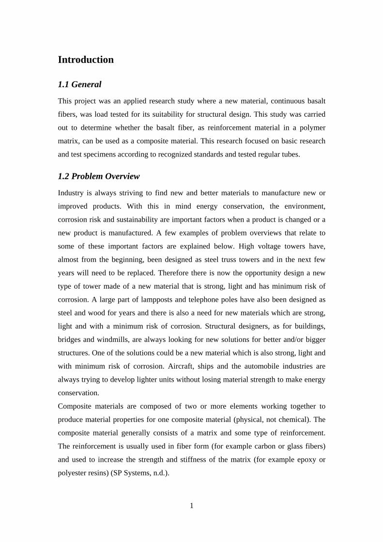
1.2 Problem Overview
Industry is always striving to find new and better materials to manufacture new or
improved products. With this in mind energy conservation, the environment,
corrosion risk and sustainability are important factors when a product is changed or a
new product is manufactured. A few examples of problem overviews that relate to
some of these important factors are explained below. High voltage towers have,
almost from the beginning, been designed as steel truss towers and in the next few
years will need to be replaced. Therefore there is now the opportunity design a new
type of tower made of a new material that is strong, light and has minimum risk of
corrosion. A large part of lampposts and telephone poles have also been designed as
steel and wood for years and there is also a need for new materials which are strong,
light and with a minimum risk of corrosion. Structural designers, as for buildings,
bridges and windmills, are always looking for new solutions for better and/or bigger
structures. One of the solutions could be a new material which is also strong, light and
with minimum risk of corrosion. Aircraft, ships and the automobile industries are
always trying to develop lighter units without losing material strength to make energy
conservation.
Composite materials are composed of two or more elements working together to
produce material properties for one composite material (physical, not chemical). The
composite material generally consists of a matrix and some type of reinforcement.
The reinforcement is usually used in fiber form (for example carbon or glass fibers)
and used to increase the strength and stiffness of the matrix (for example epoxy or
polyester resins) (SP Systems, n.d.).
2
Basalt fiber is a natural material which is produced from igneous rock called basalt
and can give great strength relative to weight (Ross, A., 2006). As has been shown in
some published papers, basalt fiber has versatile material properties (Parnas, R. &
Shaw, M., 2007; Van de Velde, K., Kiekens, P., & Van Langenhove, L., n.d.). The
aim of this thesis was to examine whether the basalt fiber as reinforcement material in
polyester resin can be used as composite material for structural design. Figures 1-1 to
1-4 show a few units which have been produced from similar material as will be
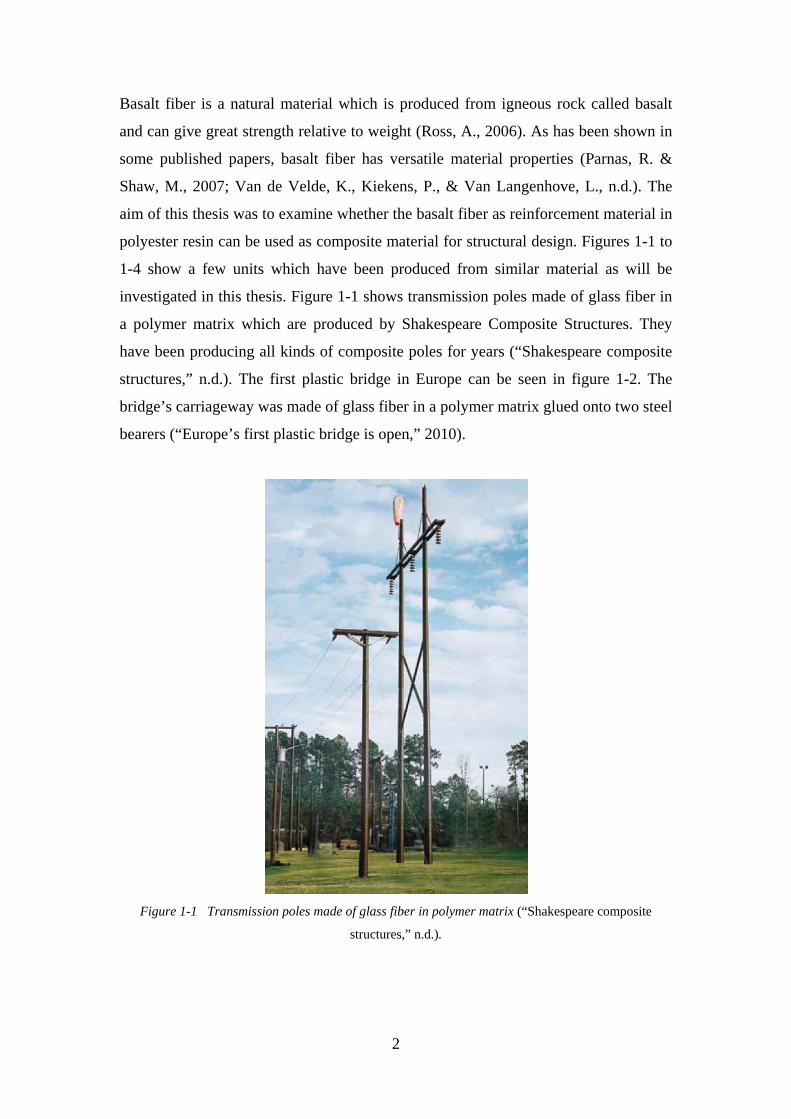
investigated in this thesis. Figure 1-1 shows transmission poles made of glass fiber in
a polymer matrix which are produced by Shakespeare Composite Structures. They
have been producing all kinds of composite poles for years (“Shakespeare composite
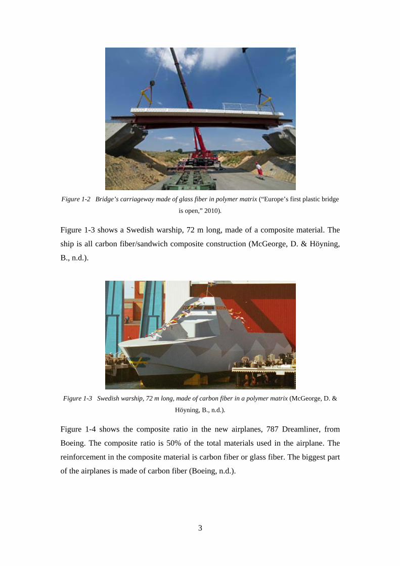
structures,” n.d.). The first plastic bridge in Europe can be seen in figure 1-2. The
bridge’s carriageway was made of glass fiber in a polymer matrix glued onto two steel
bearers (“Europe’s first plastic bridge is open,” 2010).
Figure 1-1 Transmission poles made of glass fiber in polymer matrix (“Shakespeare composite
structures,” n.d.).
3
Figure 1-2 Bridge’s carriageway made of glass fiber in polymer matrix (“Europe’s first plastic bridge
is open,” 2010).
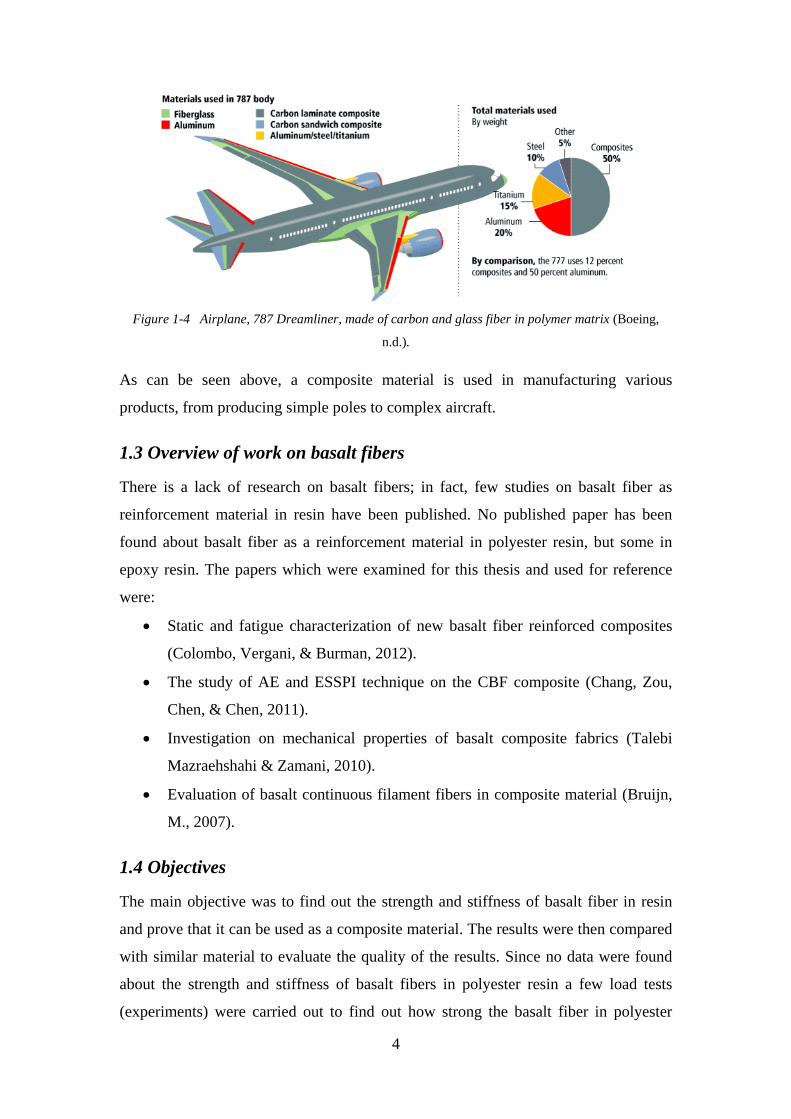
Figure 1-3 shows a Swedish warship, 72 m long, made of a composite material. The
ship is all carbon fiber/sandwich composite construction (McGeorge, D. & Höyning,
B., n.d.).
Figure 1-3 Swedish warship, 72 m long, made of carbon fiber in a polymer matrix (McGeorge, D. &
Höyning, B., n.d.).
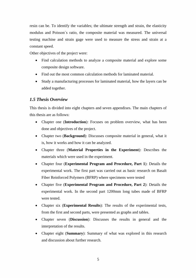
Figure 1-4 shows the composite ratio in the new airplanes, 787 Dreamliner, from
Boeing. The composite ratio is 50% of the total materials used in the airplane. The
reinforcement in the composite material is carbon fiber or glass fiber. The biggest part
of the airplanes is made of carbon fiber (Boeing, n.d.).
4
Figure 1-4 Airplane, 787 Dreamliner, made of carbon and glass fiber in polymer matrix (Boeing,
n.d.).
As can be seen above, a composite material is used in manufacturing various
products, from producing simple poles to complex aircraft.
1.3 Overview of work on basalt fibers
There is a lack of research on basalt fibers; in fact, few studies on basalt fiber as
reinforcement material in resin have been published. No published paper has been
found about basalt fiber as a reinforcement material in polyester resin, but some in
epoxy resin. The papers which were examined for this thesis and used for reference
were:
• Static and fatigue characterization of new basalt fiber reinforced composites
(Colombo, Vergani, & Burman, 2012).
• The study of AE and ESSPI technique on the CBF composite (Chang, Zou,
Chen, & Chen, 2011).
• Investigation on mechanical properties of basalt composite fabrics (Talebi
Mazraehshahi & Zamani, 2010).
• Evaluation of basalt continuous filament fibers in composite material (Bruijn,
M., 2007).
1.4 Objectives
The main objective was to find out the strength and stiffness of basalt fiber in resin
and prove that it can be used as a composite material. The results were then compared
with similar material to evaluate the quality of the results. Since no data were found
about the strength and stiffness of basalt fibers in polyester resin a few load tests
(experiments) were carried out to find out how strong the basalt fiber in polyester
5
resin can be. To identify the variables; the ultimate strength and strain, the elasticity
modulus and Poisson´s ratio, the composite material was measured. The universal
testing machine and strain gage were used to measure the stress and strain at a
constant speed.
Other objectives of the project were:
• Find calculation methods to analyze a composite material and explore some
composite design software.
• Find out the most common calculation methods for laminated material.
• Study a manufacturing processes for laminated material, how the layers can be
added together.
1.5 Thesis Overview
This thesis is divided into eight chapters and seven appendixes. The main chapters of
this thesis are as follows:
• Chapter one (Introduction): Focuses on problem overview, what has been
done and objectives of the project.
• Chapter two (Background): Discusses composite material in general, what it
is, how it works and how it can be analyzed.
• Chapter three (Material Properties in the Experiment): Describes the
materials which were used in the experiment.
• Chapter four (Experimental Program and Procedure, Part 1): Details the
experimental work. The first part was carried out as basic research on Basalt
Fiber Reinforced Polymers (BFRP) where specimens were tested
• Chapter five (Experimental Program and Procedure, Part 2): Details the
experimental work. In the second part 1200mm long tubes made of BFRP
were tested.
• Chapter six (Experimental Results): The results of the experimental tests,
from the first and second parts, were presented as graphs and tables.
• Chapter seven (Discussion): Discusses the results in general and the
interpretation of the results.
• Chapter eight (Summary): Summary of what was explored in this research
and discussion about further research.
6
Background
2.1 General
Composite materials are those which are composed of two or more elements working
together to produce material properties for this one composite material (physical, not
chemical). In a most basic and practical way a composite material consists of a matrix
and some type of reinforcement. The reinforcement is usually in fiber form and used
to increase the strength and stiffness of the matrix (SP Systems, n.d.).
2.2 Composite material
2.2.1 Resin Systems
There are three groups of most common man-made composites: Polymer Matrix
Composites, Metal Matrix Composites and Ceramic Matrix Composite (SP Systems,
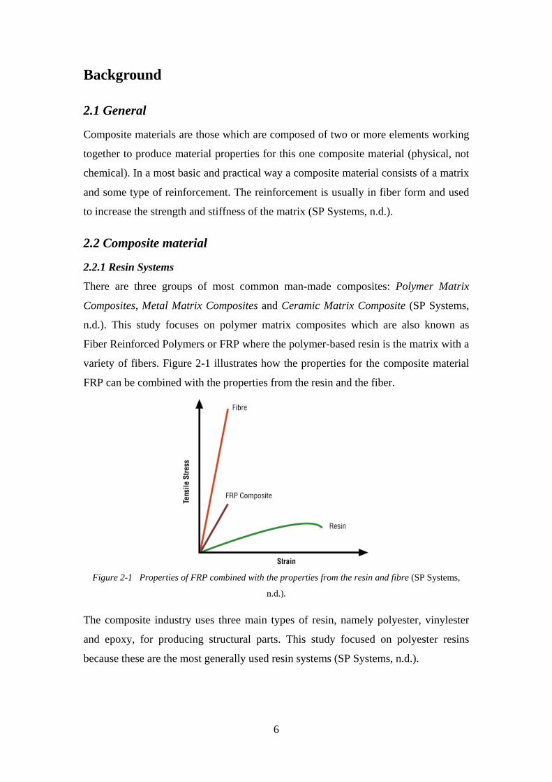
n.d.). This study focuses on polymer matrix composites which are also known as
Fiber Reinforced Polymers or FRP where the polymer-based resin is the matrix with a
variety of fibers. Figure 2-1 illustrates how the properties for the composite material
FRP can be combined with the properties from the resin and the fiber.
Figure 2-1 Properties of FRP combined with the properties from the resin and fibre (SP Systems,
n.d.).
The composite industry uses three main types of resin, namely polyester, vinylester
and epoxy, for producing structural parts. This study focused on polyester resins
because these are the most generally used resin systems (SP Systems, n.d.).
7
2.2.2 Reinforcements (fiber)
Fiber reinforcements in composite material are generally used to improve the
mechanical properties in an undiluted resin system. The most common fiber
reinforcement in resin is glass fiber, accounting for up to 99% of world production
(Árnason, P., 2007, p. 143). There are other types of fibers for reinforcement such as
carbon fiber, other plastic fibers and the newest, basalt fiber, which is examined in
this research. For this reason the study focused on basalt fiber and below the basalt
fiber is described roughly.
Basalt is an igneous rock (volcanic rock) formed in volcanic eruptions and found in
almost all countries around the world (Ross, A., 2006). The bulk of Iceland's bedrock
is basalt, which is widely used as building material in the country. Basalt is a building
material that could effectively find wider application since it is so abundant
worldwide. One suggested use would be as fiber reinforcement of resin.
The production of basalt fibers is similar to the production of glass fibers. Basalt is
quarried, crushed and washed and then melted at 1500° C (Ross, A., 2006). Next, the
molten basalt is drawn into filaments. When the filaments cool down it is transformed
into fibers (Ross, A., 2006).
Manufacturers of basalt fibers (e.g. Kamenny Vek in Russia) say that basalt fibers
have preferable mechanical properties, such as higher tensile strength, as well as a
lower manufacturing cost than glass fibers (Kamenny Vek, 2009). Kamenny Vek also
says recycling of basalt fibers is much more efficient than glass fibers and therefore
basalt fibers can be environmentally friendly (Kamenny Vek, 2009). Basalt fiber can
be classified as a sustainable material because basalt fibers are made of natural
material and when the basalt fibers in resin are recycled the same material is obtained
again as natural basalt powder (Kamenny Vek, 2009).
2.2.3 Manufacturing Processes for laminate material
A composite laminate is generally made of several composite material layers with
different fiber orientations; thus some manufacturing process is needed to add the
layers together. This section focuses on three common types of manufacturing
processes which are Hand Lay-up, Vacuum Bagging and Vacuum Infusion. All these
methods can work with various types of fiber fabrics and general resin. The fabrics
are generally made of continuous fibers which are in the form of woven or stitched
fabrics (SP Systems, n.d.).
8
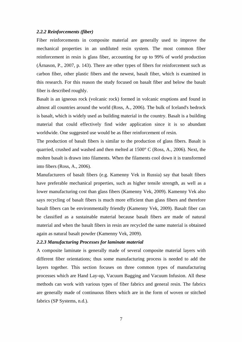
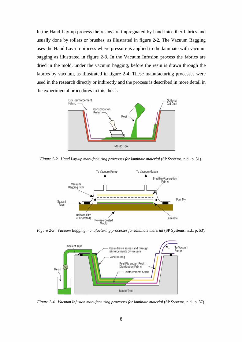
In the Hand Lay-up process the resins are impregnated by hand into fiber fabrics and
usually done by rollers or brushes, as illustrated in figure 2-2. The Vacuum Bagging
uses the Hand Lay-up process where pressure is applied to the laminate with vacuum
bagging as illustrated in figure 2-3. In the Vacuum Infusion process the fabrics are
dried in the mold, under the vacuum bagging, before the resin is drawn through the
fabrics by vacuum, as illustrated in figure 2-4. These manufacturing processes were
used in the research directly or indirectly and the process is described in more detail in
the experimental procedures in this thesis.
Figure 2-2 Hand Lay-up manufacturing processes for laminate material (SP Systems, n.d., p. 51).
Figure 2-3 Vacuum Bagging manufacturing processes for laminate material (SP Systems, n.d., p. 53).
Figure 2-4 Vacuum Infusion manufacturing processes for laminate material (SP Systems, n.d., p. 57).
9
2.3 Analytical Modeling (analysis of composite materials)
The physical behavior of composite laminate can be more complicated than other
engineering materials. The most common engineering materials are assumed to be
isotropic and homogeneous (Greene, E., n.d., p. 99). That kind of materials are
assumed to be constant throughout and the elastic properties are the same in all
direction (Staab, 1999, p. 13).
Most composite materials are nonhomogeneous and behave as anisotropic or
orthotropic materials, which means the elastic properties can be different in all
directions. For that reason it can be more complex to analyze and make a design
method for composite structures. Composite material will hereafter stand for fiber-
reinforced material in a matrix and this study focuses always on a continuous fiber
composite.
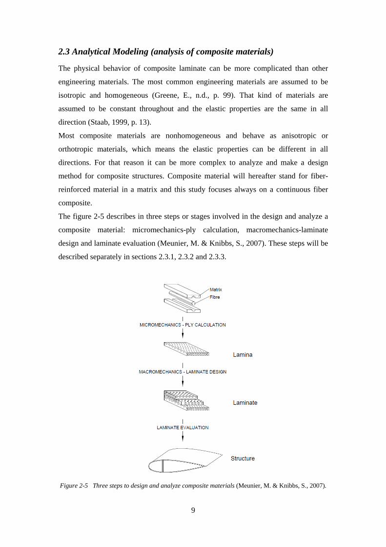
The figure 2-5 describes in three steps or stages involved in the design and analyze a
composite material: micromechanics-ply calculation, macromechanics-laminate
design and laminate evaluation (Meunier, M. & Knibbs, S., 2007). These steps will be
described separately in sections 2.3.1, 2.3.2 and 2.3.3.
Figure 2-5 Three steps to design and analyze composite materials (Meunier, M. & Knibbs, S., 2007).
10
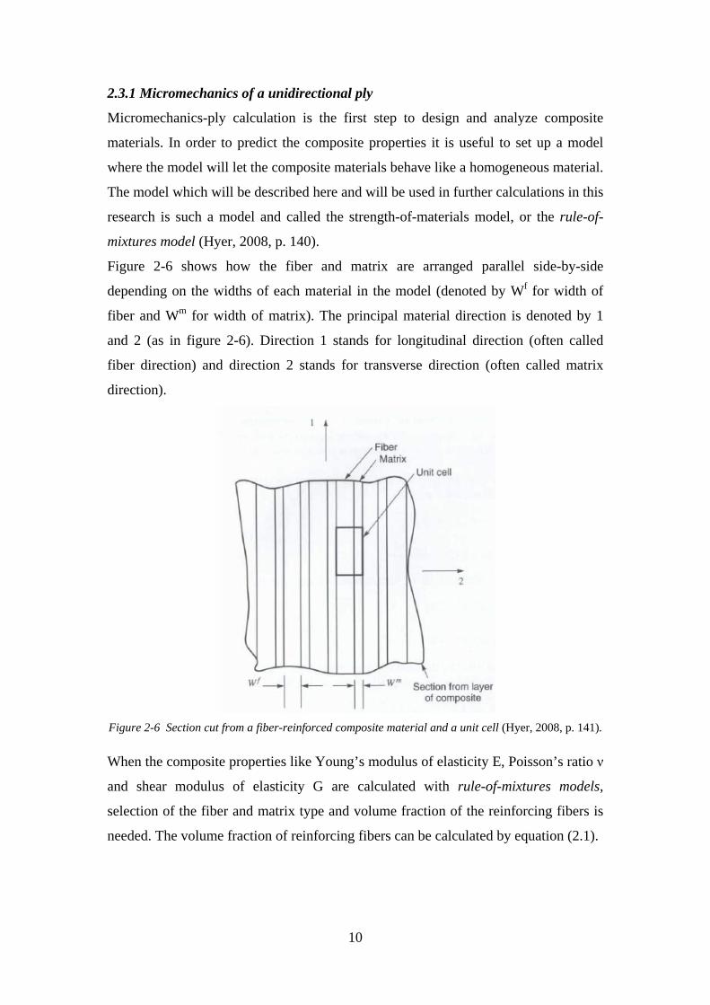
2.3.1 Micromechanics of a unidirectional ply
Micromechanics-ply calculation is the first step to design and analyze composite
materials. In order to predict the composite properties it is useful to set up a model
where the model will let the composite materials behave like a homogeneous material.
The model which will be described here and will be used in further calculations in this
research is such a model and called the strength-of-materials model, or the rule-of-
mixtures model (Hyer, 2008, p. 140).
Figure 2-6 shows how the fiber and matrix are arranged parallel side-by-side
depending on the widths of each material in the model (denoted by Wf for width of
fiber and Wm for width of matrix). The principal material direction is denoted by 1
and 2 (as in figure 2-6). Direction 1 stands for longitudinal direction (often called
fiber direction) and direction 2 stands for transverse direction (often called matrix
direction).
Figure 2-6 Section cut from a fiber-reinforced composite material and a unit cell (Hyer, 2008, p. 141).
When the composite properties like Young’s modulus of elasticity E, Poisson’s ratio ν
and shear modulus of elasticity G are calculated with rule-of-mixtures models,
selection of the fiber and matrix type and volume fraction of the reinforcing fibers is
needed. The volume fraction of reinforcing fibers can be calculated by equation (2.1).
11
𝑉𝑉𝑓𝑓 =
𝑀𝑀𝑓𝑓
𝜌𝜌𝑓𝑓�
𝑀𝑀𝑡𝑡𝑡𝑡𝑡𝑡𝑡𝑡𝑡𝑡 𝜌𝜌𝑡𝑡𝑡𝑡𝑡𝑡𝑡𝑡𝑡𝑡�
where 𝑉𝑉𝑓𝑓 = volume fraction of reinforcing fibers
𝑀𝑀𝑓𝑓 = mass of reinforcing fibers
𝜌𝜌𝑓𝑓 = density of reinforcing fibers
𝑀𝑀𝑡𝑡𝑡𝑡𝑡𝑡𝑡𝑡𝑡𝑡 = total mass (mass of reinforcing fibers plus mass of matrix)
𝜌𝜌𝑡𝑡𝑡𝑡𝑡𝑡𝑡𝑡𝑡𝑡 = total density (density of reinforcing fibers plus density of matrix)
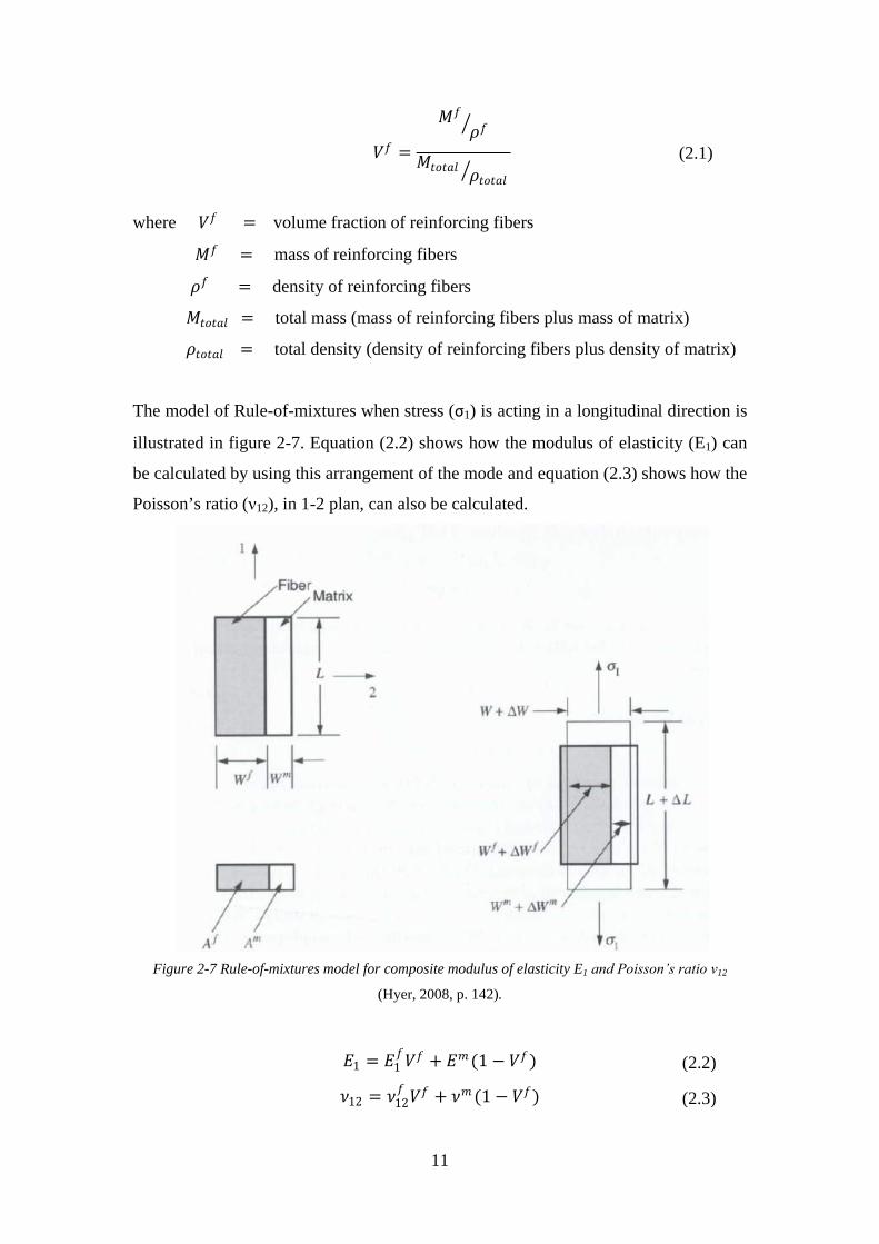
The model of Rule-of-mixtures when stress (σ1) is acting in a longitudinal direction is
illustrated in figure 2-7. Equation (2.2) shows how the modulus of elasticity (E1) can
be calculated by using this arrangement of the mode and equation (2.3) shows how the
Poisson’s ratio (ν12), in 1-2 plan, can also be calculated.
Figure 2-7 Rule-of-mixtures model for composite modulus of elasticity E1 and Poisson’s ratio ν12
(Hyer, 2008, p. 142).
𝐸𝐸1 = 𝐸𝐸1
𝑓𝑓𝑉𝑉𝑓𝑓 + 𝐸𝐸𝑚𝑚(1 − 𝑉𝑉𝑓𝑓)
𝜈𝜈12 = 𝜈𝜈12𝑓𝑓 𝑉𝑉𝑓𝑓 + 𝜈𝜈𝑚𝑚(1 − 𝑉𝑉𝑓𝑓)
(2.1)
(2.2)
(2.3)
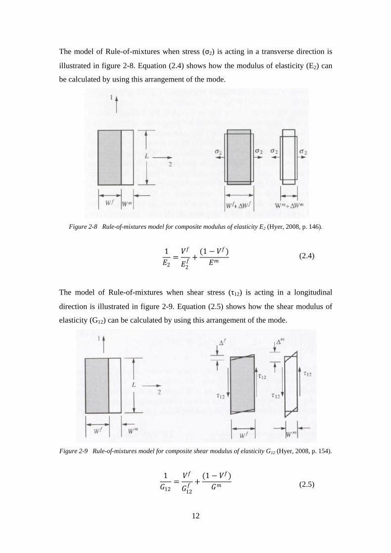
12
The model of Rule-of-mixtures when stress (σ2) is acting in a transverse direction is
illustrated in figure 2-8. Equation (2.4) shows how the modulus of elasticity (E2) can
be calculated by using this arrangement of the mode.
Figure 2-8 Rule-of-mixtures model for composite modulus of elasticity E2 (Hyer, 2008, p. 146).
1𝐸𝐸2
=𝑉𝑉𝑓𝑓
𝐸𝐸2𝑓𝑓 +
(1 − 𝑉𝑉𝑓𝑓)𝐸𝐸𝑚𝑚
The model of Rule-of-mixtures when shear stress (τ12) is acting in a longitudinal
direction is illustrated in figure 2-9. Equation (2.5) shows how the shear modulus of
elasticity (G12) can be calculated by using this arrangement of the mode.
Figure 2-9 Rule-of-mixtures model for composite shear modulus of elasticity G12 (Hyer, 2008, p. 154).
1𝐺𝐺12
=𝑉𝑉𝑓𝑓
𝐺𝐺12𝑓𝑓 +
(1 − 𝑉𝑉𝑓𝑓)𝐺𝐺𝑚𝑚
(2.4)
(2.5)
13
where: 𝐸𝐸1 = elasticity composite modulus in1 direction (longitudinal)
𝐸𝐸2 = elasticity composite modulus in 2 direction (transverse)
𝐺𝐺12 = elasticity composite shear modulus in 1-2 plane
𝐸𝐸1𝑓𝑓 = elasticity modulus of fiber in 1 direction (longitudinal)
𝐸𝐸2𝑓𝑓 = elasticity modulus of fiber in 2 direction (transverse)
𝐸𝐸𝑚𝑚 = elasticity modulus of matrix
𝐺𝐺𝑚𝑚 = elasticity shear modulus of matrix
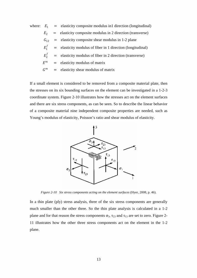
If a small element is considered to be removed from a composite material plate, then
the stresses on its six bounding surfaces on the element can be investigated in a 1-2-3
coordinate system. Figure 2-10 illustrates how the stresses act on the element surfaces
and there are six stress components, as can be seen. So to describe the linear behavior
of a composite material nine independent composite properties are needed, such as
Young’s modulus of elasticity, Poisson’s ratio and shear modulus of elasticity.
Figure 2-10 Six stress components acting on the element surfaces (Hyer, 2008, p. 46).
In a thin plate (ply) stress analysis, three of the six stress components are generally
much smaller than the other three. So the thin plate analysis is calculated in a 1-2
plane and for that reason the stress components σ3, τ23 and τ13 are set to zero. Figure 2-
11 illustrates how the other three stress components act on the element in the 1-2
plane.
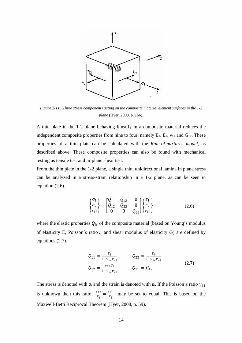
14
Figure 2-11 Three stress components acting on the composite material element surfaces in the 1-2
plane (Hyer, 2008, p. 166).
A thin plate in the 1-2 plane behaving linearly in a composite material reduces the
independent composite properties from nine to four, namely E1, E2, ν12 and G12. These
properties of a thin plate can be calculated with the Rule-of-mixtures model, as
described above. These composite properties can also be found with mechanical
testing as tensile test and in-plane shear test.
From the thin plate in the 1-2 plane, a single thin, unidirectional lamina in plane stress
can be analyzed in a stress-strain relationship in a 1-2 plane, as can be seen in
equation (2.6).
�𝜎𝜎1𝜎𝜎2𝜏𝜏12
� = �𝑄𝑄11 𝑄𝑄12 0𝑄𝑄12 𝑄𝑄22 0
0 0 𝑄𝑄66
� �𝜀𝜀1𝜀𝜀2𝛾𝛾12
�
where the elastic properties 𝑄𝑄𝑖𝑖𝑖𝑖 of the composite material (based on Young’s modulus
of elasticity E, Poisson´s ratio ν and shear modulus of elasticity G) are defined by
equations (2.7).
𝑄𝑄11 = 𝐸𝐸1
1−𝜈𝜈12𝜈𝜈21 𝑄𝑄22 = 𝐸𝐸2
1−𝜈𝜈12𝜈𝜈21
𝑄𝑄12 = 𝜈𝜈12𝐸𝐸11−𝜈𝜈12𝜈𝜈21
𝑄𝑄11 = 𝐺𝐺12
The stress is denoted with σi and the strain is denoted with ɛi. If the Poisson’s ratio 𝜈𝜈21
is unknown then this ratio 𝜈𝜈12𝐸𝐸1
= 𝜈𝜈21𝐸𝐸2
may be set to equal. This is based on the
Maxwell-Betti Reciprocal Theorem (Hyer, 2008, p. 59).
(2.6)
(2.7) (2.7)
15
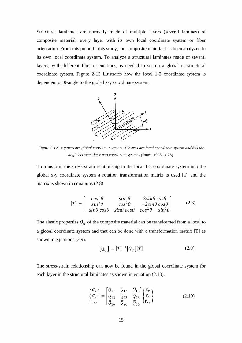
Structural laminates are normally made of multiple layers (several laminas) of
composite material, every layer with its own local coordinate system or fiber
orientation. From this point, in this study, the composite material has been analyzed in
its own local coordinate system. To analyze a structural laminates made of several
layers, with different fiber orientations, is needed to set up a global or structural
coordinate system. Figure 2-12 illustrates how the local 1-2 coordinate system is
dependent on θ-angle to the global x-y coordinate system.
Figure 2-12 x-y axes are global coordinate system, 1-2 axes are local coordinate system and θ is the
angle between these two coordinate systems (Jones, 1998, p. 75).
To transform the stress-strain relationship in the local 1-2 coordinate system into the
global x-y coordinate system a rotation transformation matrix is used [T] and the
matrix is shown in equations (2.8).
[𝑇𝑇] = �𝑐𝑐𝑡𝑡𝑠𝑠2𝜃𝜃 𝑠𝑠𝑖𝑖𝑠𝑠2𝜃𝜃 2𝑠𝑠𝑖𝑖𝑠𝑠𝜃𝜃 𝑐𝑐𝑡𝑡𝑠𝑠𝜃𝜃𝑠𝑠𝑖𝑖𝑠𝑠2𝜃𝜃 𝑐𝑐𝑡𝑡𝑠𝑠2𝜃𝜃 −2𝑠𝑠𝑖𝑖𝑠𝑠𝜃𝜃 𝑐𝑐𝑡𝑡𝑠𝑠𝜃𝜃
−𝑠𝑠𝑖𝑖𝑠𝑠𝜃𝜃 𝑐𝑐𝑡𝑡𝑠𝑠𝜃𝜃 𝑠𝑠𝑖𝑖𝑠𝑠𝜃𝜃 𝑐𝑐𝑡𝑡𝑠𝑠𝜃𝜃 𝑐𝑐𝑡𝑡𝑠𝑠2𝜃𝜃 − 𝑠𝑠𝑖𝑖𝑠𝑠2𝜃𝜃�
The elastic properties 𝑄𝑄𝑖𝑖𝑖𝑖 of the composite material can be transformed from a local to
a global coordinate system and that can be done with a transformation matrix [T] as
shown in equations (2.9).
�𝑄𝑄�𝑖𝑖𝑖𝑖 � = [𝑇𝑇]−1�𝑄𝑄𝑖𝑖𝑖𝑖 �[𝑇𝑇]
The stress-strain relationship can now be found in the global coordinate system for
each layer in the structural laminates as shown in equation (2.10).
�𝜎𝜎𝑥𝑥𝜎𝜎𝑦𝑦𝜏𝜏𝑥𝑥𝑦𝑦
� = �𝑄𝑄�11 𝑄𝑄�12 𝑄𝑄�16𝑄𝑄�12 𝑄𝑄�22 𝑄𝑄�26𝑄𝑄�16 𝑄𝑄�26 𝑄𝑄�66
� �𝜀𝜀𝑥𝑥𝜀𝜀𝑥𝑥𝛾𝛾𝑥𝑥𝑦𝑦
�
(2.8)
(2.9)
(2.10)
16
2.3.2 Classical Laminate Theory
Macromechanics-laminate design is the second step to design and analyze composite
materials. There are many macromechanical theories that have been presented in
recent years to analyze a composite laminate. A few of them are shown here below.
Two-dimensional theory (Manjunatha & Kant, 1992)
• Classical Laminate theory (CLT)
• Higher-order shear deformation theory (HOST)
Three-dimensional theory (Kant, T., 2010)
• Finite element model
One of the most prevalent models to analyze a composite laminate is the Classical
Laminate Theory, or CLT. The theory is explained here below and used for further
calculations in this study.
CLT is a first-order shear deformation theory and based on the Kirchhoff hypothesis.
It was in the 1800s when the Kirchhoff hypothesis was originally introduced (Hyer,
2008, p. 302). The first paper about CLT was published by Reissner 1961 (Reissner &
Stavsky, 1961). The layers in the laminate do not have to be made of the same
composite materials. The layers can be from one up to several hundred layers in each
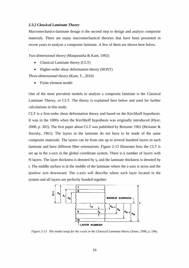
laminate and have different fiber orientations. Figure 2-13 illustrates how the CLT is
set up in the z-axis in the global coordinate system. There is k number of layers with
N layers. The layer thickness is denoted by tk and the laminate thickness is denoted by
t. The middle surface is in the middle of the laminate where the z-axis is zeros and the
positive axis downward. The z-axis will describe where each layer located in the
system and all layers are perfectly bonded together.
Figure 2-13 The model setup for the z-axis in the Classical Laminate theory (Jones, 1998, p. 196).
17
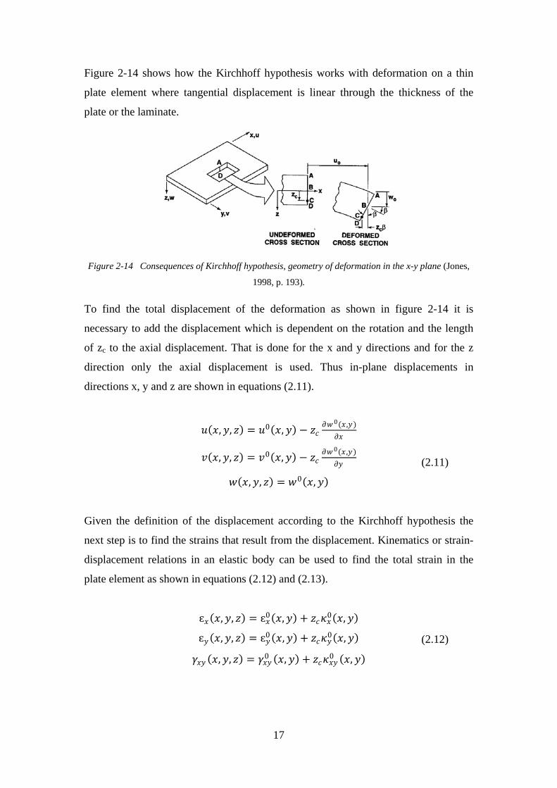
Figure 2-14 shows how the Kirchhoff hypothesis works with deformation on a thin
plate element where tangential displacement is linear through the thickness of the
plate or the laminate.
Figure 2-14 Consequences of Kirchhoff hypothesis, geometry of deformation in the x-y plane (Jones,
1998, p. 193).
To find the total displacement of the deformation as shown in figure 2-14 it is
necessary to add the displacement which is dependent on the rotation and the length
of zc to the axial displacement. That is done for the x and y directions and for the z
direction only the axial displacement is used. Thus in-plane displacements in
directions x, y and z are shown in equations (2.11).
𝑏𝑏(𝑥𝑥, 𝑦𝑦, 𝑧𝑧) = 𝑏𝑏0(𝑥𝑥,𝑦𝑦) − 𝑧𝑧𝑐𝑐𝜕𝜕𝑤𝑤0(𝑥𝑥 ,𝑦𝑦)
𝜕𝜕𝑥𝑥
𝑣𝑣(𝑥𝑥, 𝑦𝑦, 𝑧𝑧) = 𝑣𝑣0(𝑥𝑥,𝑦𝑦) − 𝑧𝑧𝑐𝑐𝜕𝜕𝑤𝑤0(𝑥𝑥 ,𝑦𝑦)
𝜕𝜕𝑦𝑦
𝑤𝑤(𝑥𝑥,𝑦𝑦, 𝑧𝑧) = 𝑤𝑤0(𝑥𝑥, 𝑦𝑦)
Given the definition of the displacement according to the Kirchhoff hypothesis the
next step is to find the strains that result from the displacement. Kinematics or strain-
displacement relations in an elastic body can be used to find the total strain in the
plate element as shown in equations (2.12) and (2.13).
ɛ𝑥𝑥(𝑥𝑥,𝑦𝑦, 𝑧𝑧) = ɛ𝑥𝑥0(𝑥𝑥,𝑦𝑦) + 𝑧𝑧𝑐𝑐𝜅𝜅𝑥𝑥0(𝑥𝑥, 𝑦𝑦)
ɛ𝑦𝑦(𝑥𝑥,𝑦𝑦, 𝑧𝑧) = ɛ𝑦𝑦0 (𝑥𝑥,𝑦𝑦) + 𝑧𝑧𝑐𝑐𝜅𝜅𝑦𝑦0(𝑥𝑥,𝑦𝑦)
𝛾𝛾𝑥𝑥𝑦𝑦 (𝑥𝑥, 𝑦𝑦, 𝑧𝑧) = 𝛾𝛾𝑥𝑥𝑦𝑦0 (𝑥𝑥, 𝑦𝑦) + 𝑧𝑧𝑐𝑐𝜅𝜅𝑥𝑥𝑦𝑦0 (𝑥𝑥, 𝑦𝑦)
(2.11)
(2.12)
18
with:
ɛ𝑥𝑥0(𝑥𝑥, 𝑦𝑦) = 𝜕𝜕𝑏𝑏0(𝑥𝑥 ,𝑦𝑦)𝜕𝜕𝑥𝑥
and 𝜅𝜅𝑥𝑥0(𝑥𝑥,𝑦𝑦) = −𝜕𝜕2𝑤𝑤0(𝑥𝑥 ,𝑦𝑦)𝜕𝜕𝑥𝑥2
ɛ𝑦𝑦0 (𝑥𝑥, 𝑦𝑦) = 𝜕𝜕𝑣𝑣0(𝑥𝑥 ,𝑦𝑦)𝜕𝜕𝑦𝑦
and 𝜅𝜅𝑦𝑦0(𝑥𝑥,𝑦𝑦) = −𝜕𝜕2𝑤𝑤0(𝑥𝑥 ,𝑦𝑦)𝜕𝜕𝑦𝑦2
𝛾𝛾𝑥𝑥𝑦𝑦0 (𝑥𝑥,𝑦𝑦) = 𝜕𝜕𝑣𝑣0(𝑥𝑥 ,𝑦𝑦)𝜕𝜕𝑥𝑥
+ 𝜕𝜕𝑏𝑏0(𝑥𝑥 ,𝑦𝑦)𝜕𝜕𝑦𝑦
and 𝜅𝜅𝑥𝑥𝑦𝑦0 (𝑥𝑥, 𝑦𝑦) = −2 𝜕𝜕2𝑤𝑤0(𝑥𝑥 ,𝑦𝑦)𝜕𝜕𝑥𝑥𝜕𝜕𝑦𝑦
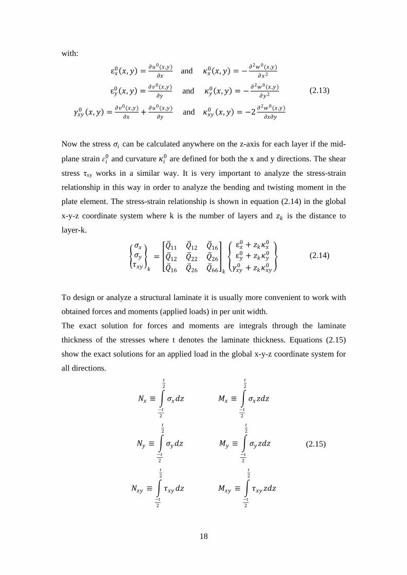
Now the stress 𝜎𝜎𝑖𝑖 can be calculated anywhere on the z-axis for each layer if the mid-
plane strain ɛ𝑖𝑖0 and curvature 𝜅𝜅𝑖𝑖0 are defined for both the x and y directions. The shear
stress τxy works in a similar way. It is very important to analyze the stress-strain
relationship in this way in order to analyze the bending and twisting moment in the
plate element. The stress-strain relationship is shown in equation (2.14) in the global
x-y-z coordinate system where k is the number of layers and 𝑧𝑧𝑘𝑘 is the distance to
layer-k.
�𝜎𝜎𝑥𝑥𝜎𝜎𝑦𝑦𝜏𝜏𝑥𝑥𝑦𝑦
�𝑘𝑘
= �𝑄𝑄�11 𝑄𝑄�12 𝑄𝑄�16𝑄𝑄�12 𝑄𝑄�22 𝑄𝑄�26𝑄𝑄�16 𝑄𝑄�26 𝑄𝑄�66
�
𝑘𝑘
�ɛ𝑥𝑥0 + 𝑧𝑧𝑘𝑘𝜅𝜅𝑥𝑥0
ɛ𝑦𝑦0 + 𝑧𝑧𝑘𝑘𝜅𝜅𝑦𝑦0
𝛾𝛾𝑥𝑥𝑦𝑦0 + 𝑧𝑧𝑘𝑘𝜅𝜅𝑥𝑥𝑦𝑦0�
To design or analyze a structural laminate it is usually more convenient to work with
obtained forces and moments (applied loads) in per unit width.
The exact solution for forces and moments are integrals through the laminate
thickness of the stresses where t denotes the laminate thickness. Equations (2.15)
show the exact solutions for an applied load in the global x-y-z coordinate system for
all directions.
𝑁𝑁𝑥𝑥 ≡ �𝜎𝜎𝑥𝑥𝑑𝑑𝑧𝑧
𝑡𝑡2
−𝑡𝑡2
𝑀𝑀𝑥𝑥 ≡ �𝜎𝜎𝑥𝑥𝑧𝑧𝑑𝑑𝑧𝑧
𝑡𝑡2
−𝑡𝑡2
𝑁𝑁𝑦𝑦 ≡ �𝜎𝜎𝑦𝑦𝑑𝑑𝑧𝑧
𝑡𝑡2
−𝑡𝑡2
𝑀𝑀𝑦𝑦 ≡ �𝜎𝜎𝑦𝑦𝑧𝑧𝑑𝑑𝑧𝑧
𝑡𝑡2
−𝑡𝑡2
𝑁𝑁𝑥𝑥𝑦𝑦 ≡ �𝜏𝜏𝑥𝑥𝑦𝑦𝑑𝑑𝑧𝑧
𝑡𝑡2
−𝑡𝑡2
𝑀𝑀𝑥𝑥𝑦𝑦 ≡ �𝜏𝜏𝑥𝑥𝑦𝑦 𝑧𝑧𝑑𝑑𝑧𝑧
𝑡𝑡2
−𝑡𝑡2
(2.13)
(2.14)
(2.15)
19
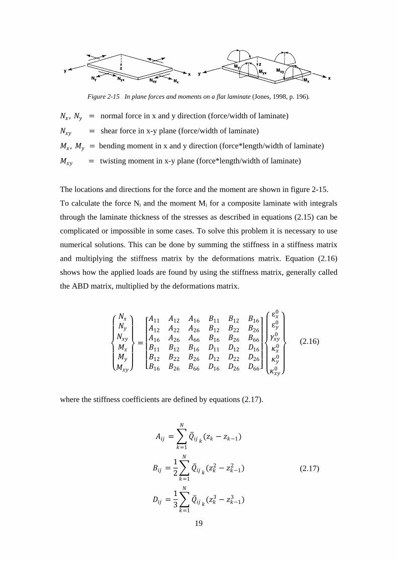
Figure 2-15 In plane forces and moments on a flat laminate (Jones, 1998, p. 196).
𝑁𝑁𝑥𝑥 , 𝑁𝑁𝑦𝑦 = normal force in x and y direction (force/width of laminate)
𝑁𝑁𝑥𝑥𝑦𝑦 = shear force in x-y plane (force/width of laminate)
𝑀𝑀𝑥𝑥 , 𝑀𝑀𝑦𝑦 = bending moment in x and y direction (force*length/width of laminate)
𝑀𝑀𝑥𝑥𝑦𝑦 = twisting moment in x-y plane (force*length/width of laminate)
The locations and directions for the force and the moment are shown in figure 2-15.
To calculate the force Ni and the moment Mi for a composite laminate with integrals
through the laminate thickness of the stresses as described in equations (2.15) can be
complicated or impossible in some cases. To solve this problem it is necessary to use
numerical solutions. This can be done by summing the stiffness in a stiffness matrix
and multiplying the stiffness matrix by the deformations matrix. Equation (2.16)
shows how the applied loads are found by using the stiffness matrix, generally called
the ABD matrix, multiplied by the deformations matrix.
⎩⎪⎪⎨
⎪⎪⎧𝑁𝑁𝑥𝑥𝑁𝑁𝑦𝑦𝑁𝑁𝑥𝑥𝑦𝑦𝑀𝑀𝑥𝑥𝑀𝑀𝑦𝑦𝑀𝑀𝑥𝑥𝑦𝑦⎭
⎪⎪⎬
⎪⎪⎫
=
⎣⎢⎢⎢⎢⎡𝐴𝐴11 𝐴𝐴12 𝐴𝐴16𝐴𝐴12 𝐴𝐴22 𝐴𝐴26𝐴𝐴16 𝐴𝐴26 𝐴𝐴66
𝐵𝐵11 𝐵𝐵12 𝐵𝐵16𝐵𝐵12 𝐵𝐵22 𝐵𝐵26𝐵𝐵16 𝐵𝐵26 𝐵𝐵66
𝐵𝐵11 𝐵𝐵12 𝐵𝐵16𝐵𝐵12 𝐵𝐵22 𝐵𝐵26𝐵𝐵16 𝐵𝐵26 𝐵𝐵66
𝐷𝐷11 𝐷𝐷12 𝐷𝐷16𝐷𝐷12 𝐷𝐷22 𝐷𝐷26𝐷𝐷16 𝐷𝐷26 𝐷𝐷66⎦
⎥⎥⎥⎥⎤
⎩⎪⎪⎨
⎪⎪⎧ ɛ𝑥𝑥0
ɛ𝑦𝑦0
𝛾𝛾𝑥𝑥𝑦𝑦0
𝜅𝜅𝑥𝑥0
𝜅𝜅𝑦𝑦0
𝜅𝜅𝑥𝑥𝑦𝑦0 ⎭⎪⎪⎬
⎪⎪⎫
where the stiffness coefficients are defined by equations (2.17).
𝐴𝐴𝑖𝑖𝑖𝑖 = �𝑄𝑄�𝑖𝑖𝑖𝑖 𝑘𝑘(𝑧𝑧𝑘𝑘 − 𝑧𝑧𝑘𝑘−1)𝑁𝑁
𝑘𝑘=1
𝐵𝐵𝑖𝑖𝑖𝑖 =12�𝑄𝑄�𝑖𝑖𝑖𝑖 𝑘𝑘(𝑧𝑧𝑘𝑘2 − 𝑧𝑧𝑘𝑘−1
2 )𝑁𝑁
𝑘𝑘=1
𝐷𝐷𝑖𝑖𝑖𝑖 =13�𝑄𝑄�𝑖𝑖𝑖𝑖 𝑘𝑘(𝑧𝑧𝑘𝑘3 − 𝑧𝑧𝑘𝑘−1
3 )𝑁𝑁
𝑘𝑘=1
(2.16)
(2.17)
20
The Aij are extensional stiffnesses, the Bij bending-extension coupling stiffnesses and
Dij are bending stiffnesses (Jones, 1998, p. 198).
“The ABD matrix defines a relationship between the stress resultants (i.e. loads)
applied to a laminate, and the reference surface strains and curvatures (i.e.,
deformations). This form is a direct result of the Kirchhoff hypothesis, the plane-stress
assumption, and the definition of the stress resultants. The laminate stiffness matrix
involves everything that is used to define the laminate-layer material properties, fiber
orientation, thickness, and location.” (Hyer, 2008, p. 323).
2.3.3 Failure theories
The third step is to evaluate the laminate by using the macromechanical failure
theories. The failure theories always examine one layer in the laminate so failure
theories have to look at all layers one by one. This section will introduce three types
of failure theories and they will be the maximum stress theory, the maximum strain
theory and the interactive failure theories.
All composite materials have a certain strength, expressed as stress or strain. When
the applied load is larger than the ultimate strength of the composite material the
material will fail. This can be avoided by using the failure theories to find out if the
composite material will fail or not.
To use these failure theories it is necessary to find the ultimate strength from uniaxial
tension and compression tests and these values can be:
𝐹𝐹1𝑇𝑇: Tensile failure strength in the 1 direction (longitudinal)
𝐹𝐹1𝐶𝐶: Compressive failure strength in the 1 direction (longitudinal)
𝐹𝐹2𝑇𝑇: Tensile failure strength in the 2 direction (transverse)
𝐹𝐹2𝐶𝐶: Compressive failure strength in the 2 direction (transverse)
𝐹𝐹12𝑆𝑆 : Shear failure strength in the 1-2 plane (longitudinal shear failure)
Maximum Stress Theory
Maximum stress theory was first suggested by C. F. Jenkins in 1920 and that was for
a failure of orthotropic materials (Staab, 1999, p. 144).
There are three models of failure in the maximum stress theory and they are
longitudinal failure, transverse failure and shear failure.
21
Longitudinal failure occurs when 𝜎𝜎1 ≥ 𝐹𝐹1𝑇𝑇 (fiber break) or 𝜎𝜎1 ≤ 𝐹𝐹1
𝐶𝐶 (fiber crushing or
kinking).
Transverse failure occurs when 𝜎𝜎2 ≥ 𝐹𝐹2𝑇𝑇 (matrix crack) or 𝜎𝜎2 ≤ 𝐹𝐹2
𝐶𝐶 (fiber and matrix
crushing or matrix yielding).
Shear failure occurs when |𝜏𝜏12| ≥ |𝐹𝐹12𝑆𝑆 | (matrix shear crack).
Maximum Strain Theory
Maximum strain theory is similar to maximum stress theory and the only difference
between these two theories is the impact from the Poisson’s ratio part of the
calculations.
Ultimate strains are calculated with the strength failure divided by Young’s modulus,
as illustrated in equations (2.18).
ɛ1𝑇𝑇𝑚𝑚𝑡𝑡𝑥𝑥 = 𝐹𝐹1
𝑇𝑇
𝐸𝐸1 ɛ1
𝐶𝐶𝑚𝑚𝑡𝑡𝑥𝑥 = 𝐹𝐹1𝐶𝐶
𝐸𝐸1
ɛ2𝑇𝑇𝑚𝑚𝑡𝑡𝑥𝑥 = 𝐹𝐹2
𝑇𝑇
𝐸𝐸2 ɛ2
𝐶𝐶𝑚𝑚𝑡𝑡𝑥𝑥 = 𝐹𝐹2𝐶𝐶
𝐸𝐸2 𝛾𝛾12
𝑆𝑆𝑚𝑚𝑡𝑡𝑥𝑥 = 𝐹𝐹12𝑆𝑆
𝐺𝐺12
The strains are calculated for the composite material in the local coordinate system as
illustrated in equations (2.19).
ɛ1 = 𝜎𝜎1−𝜈𝜈12𝜎𝜎2𝐸𝐸1
ɛ2 = 𝜎𝜎2−𝜈𝜈21𝜎𝜎1𝐸𝐸2
𝛾𝛾12 = 𝜏𝜏12𝐺𝐺12
There are also three models of failure in the maximum strain theory as in the
maximum stress theory, longitudinal failure, transverse failure and shear failure.
Longitudinal failure occurs when ɛ1 ≥ ɛ1𝑇𝑇𝑚𝑚𝑡𝑡𝑥𝑥 or ɛ1 ≤ ɛ1
𝐶𝐶𝑚𝑚𝑡𝑡𝑥𝑥
Transverse failure occurs when ɛ2 ≥ ɛ2𝑇𝑇𝑚𝑚𝑡𝑡𝑥𝑥 or ɛ2 ≤ ɛ2
𝐶𝐶𝑚𝑚𝑡𝑡𝑥𝑥
Shear failure occurs when |𝛾𝛾12| ≥ |𝛾𝛾12𝑆𝑆𝑚𝑚𝑡𝑡𝑥𝑥 |
Interactive failure theories
The interactive failure criterion was introduced, in 1950, by Hill for the first time and
since then others have modified his theory (Staab, 1999, pp. 152–153). These theories
may be classified into two categories and some of them are listed below (Staab, 1999,
p. 153).
(2.18)
(2.19)
22
1) Criterion: 𝐹𝐹𝑖𝑖𝑖𝑖 𝜎𝜎𝑖𝑖𝜎𝜎𝑖𝑖 = 1 Theory: Ashkenazi, Chamis, Fischer, Tsai-Hill and
Norris.
2) Criterion: 𝐹𝐹𝑖𝑖𝑖𝑖 𝜎𝜎𝑖𝑖𝜎𝜎𝑖𝑖 + 𝐹𝐹𝑖𝑖𝜎𝜎𝑖𝑖 = 1 Theory: Cowin, Hoffman, Malmeister, Marin,
Tsai-Wu and Gol’denblat-Kopnov.
This section describes one theory from each category, Tsai-Hill and Tsai-Wu, with a
rough description of how they work.
Tsai-Hill Theory
The Tsai-Hill theory is an extension of the von Mises theories and is an interactive
stress-based criterion and indicates whether or not there is failure (Staab, 1999, p.
155).
The criterion for the Tsai- Hill theory is 𝐹𝐹𝑖𝑖𝑖𝑖 𝜎𝜎𝑖𝑖𝜎𝜎𝑖𝑖 = 1 and for plane stress the failure
theory is written as:
Failure occurs when 𝜎𝜎1
2
𝑆𝑆12 −
𝜎𝜎1𝜎𝜎2𝑆𝑆1
2 + 𝜎𝜎22
𝑆𝑆22 + 𝜏𝜏12
2
𝐹𝐹12𝑆𝑆 2 ≥ 1.0
The following condition has to be satisfied: if 𝜎𝜎1 ≥ 0 then 𝑆𝑆1 = 𝐹𝐹1𝑇𝑇
if 𝜎𝜎1 < 0 then 𝑆𝑆1 = 𝐹𝐹1𝐶𝐶
if 𝜎𝜎2 ≥ 0 then 𝑆𝑆2 = 𝐹𝐹2𝑇𝑇
if 𝜎𝜎2 < 0 then 𝑆𝑆2 = 𝐹𝐹2𝐶𝐶
Tsai-Wu Theory
The Tsai-Wu theory is an interactive stress-based criterion and indicates whether or
not there is failure. In this theory there is only one model of failure and the criterion
for the Tsai-Wu theory is 𝐹𝐹𝑖𝑖𝜎𝜎𝑖𝑖 + 𝐹𝐹𝑖𝑖𝑖𝑖 𝜎𝜎𝑖𝑖𝜎𝜎𝑖𝑖 = 1 𝑖𝑖, 𝑖𝑖 = 1,2, . . . ,6. For plane stress the
failure theory is written as:
Failure occurs when 𝐹𝐹11𝜎𝜎12 + 2𝐹𝐹12𝜎𝜎1𝜎𝜎2 + 𝐹𝐹22𝜎𝜎2
2 + 𝐹𝐹66𝜏𝜏122 + 𝐹𝐹1𝜎𝜎1 + 𝐹𝐹2𝜎𝜎2 ≥ 1.0
F1, F11, F2 and F22 are determine by using uniaxial tension and compressions tests and
the results from that calculation can be seen in equations (2.20).
23
𝐹𝐹11 = 1𝐹𝐹1𝑇𝑇𝐹𝐹1
𝐶𝐶 𝐹𝐹1 = 1𝐹𝐹1𝑇𝑇 −
1𝐹𝐹1𝐶𝐶
𝐹𝐹22 = 1𝐹𝐹2𝑇𝑇𝐹𝐹2
𝐶𝐶 𝐹𝐹2 = 1𝐹𝐹2𝑇𝑇 −
1𝐹𝐹2𝐶𝐶 𝐹𝐹66 = 1
𝐹𝐹2𝑇𝑇𝐹𝐹2
𝐶𝐶
To determine the F12 a biaxial tension test is used, but it can be difficult to perform a
biaxial tension test and it will not give an exact solution. So there is another solution
that can be used and that is 𝐹𝐹12 = 𝐹𝐹12∗ �𝐹𝐹11𝐹𝐹22 where 𝐹𝐹12
∗ is user-specified constant
and this constant is best defined as 𝐹𝐹12∗ = −1
2� (Staab, 1999, p. 162).
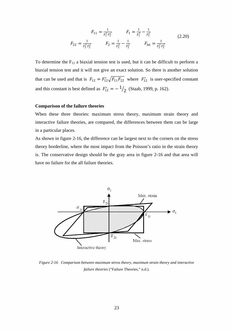
Comparison of the failure theories
When these three theories: maximum stress theory, maximum strain theory and
interactive failure theories, are compared, the differences between them can be large
in a particular places.
As shown in figure 2-16, the difference can be largest next to the corners on the stress
theory borderline, where the most impact from the Poisson’s ratio in the strain theory
is. The conservative design should be the gray area in figure 2-16 and that area will
have no failure for the all failure theories.
Figure 2-16 Comparison between maximum stress theory, maximum strain theory and interactive
failure theories (“Failure Theories,” n.d.).
(2.20)
24
2.3.4 Laminate Design Software
There are a number of software programs which are used to analyze and design a
composite material. The National Composites Network published in 2006 a report,
named Design Tools for Fibre Reinforced Polymer Structures (Meunier, M. &
Knibbs, S., 2007). The purpose of the report was to help composite design engineers
to select and identify the best design tool for their need.
Nine laminate design tools were compared and they were The Laminator Versions
3.6, ESDU Composites Series, LAP Version 4.0, CoDA Version 3.3, Kolibri Version
3, ESAComp Version 3.5, Composite Star Version 2.0, Composite Pro Version 3.0
and Think Composites. All the software programs used micromechanics-ply
calculations and several of them used the rule-of-mixtures model. All the software
programs used Classical Laminate Theory in the macromechanics-laminate design.
All the software programs used a failure theories maximum stress, maximum strain,
Tsai-Hill, Tsai-Wu, and several others in some cases. The summary from the report
Design Tools for Fibre Reinforced Polymer Structures shows that the theories which
have been described in this thesis are commonly used in laminate design tools.
2.4 Test Methods
In basic research where material properties are tested for a new material it is
necessary to use recognized standards, such as ASTM, to compare other material
properties on same basis. This study performed basic research on material properties
and ASTM standards are used. ASTM are international standards and stands for the
American Society for Testing and Materials. In 1898 ASTM was created by chemists
and engineers and in 2001, the Society became known as ASTM (ASTM
International, 2012).
The standard test methods that used in this research were:
1) To find the volume fraction of reinforcing fibers in the composite material
using: ASTM D3171 Constituent Content of Composite Materials (ASTM
D3171, 2000).
2) To perform a uniaxial tension tests using: ASTM D3039 Tensile Properties of
Polymer Matrix Composite Materials (ASTM D3039, 2000).
3) To perform a uniaxial compression tests using a combination of two methods:
ASTM D695 Compressive Properties of Rigid Plastics (ASTM D695, 2002)
and ASTM D3410 Compressive Properties of Polymer Matrix Composite
25
Materials with Unsupported Gage Section by Shear Loading (ASTM D3410,
2003).
4) To perform a uniaxial in-plane shear test using: ASTM D3518 In-plane Shear
Response of Polymer Matrix Composite Materials by Tensile Test of a ±45°
Laminate (ASTM D3518, 1994).
5) To perform a pin bearing test using: ASTM D5961 Bering Response of
Polymer Matrix Composite Laminates (ASTM D5961, 2001).
6) To perform the Young’s Modulus in the uniaxial test using: ASTM E111
Young’s Modulus, Tangent Modulus, and Chord Modulus (ASTM E111,
1997).
7) To perform the Poisson’s Ratio using: ASTM E132 Poisson’s Ratio at Room
Temperature (ASTM E132, 2004).
2.5 Summary
• A composite material is composed of at two or more elements working
together.
• Composite material consists of a matrix and some type of reinforcement.
• The matrix can be a polymer-based resin and this study focused on polyester.
• The reinforcement can be continuous fibers which are in the form of woven or
stitched fabrics and this study will focused on basalt fibers.
• Manufacturing processes for laminate material can be Hand Lay-up, Vacuum
Bagging and Vacuum Infusion.
• The rule-of-mixtures model can be used to calculate the properties for a
composite material.
• Classical Laminate Theory can be used to calculate a laminate material.
• The failure theories can be used to evaluate the laminate and the theories can
be maximum stress theory, maximum strain theory, Tsai-Hill and Tsai-Wu.
• The theories which have been described in this section are commonly used in
laminate design tools.
• ASTM standards can be used for basic research, such as uniaxial tension and
compression tests for composite material.
26
Material Properties in the Experiment
3.1 General
The experimental programs were divided into two parts. The first part was carried out
as basic research on Basalt Fiber Reinforced Polymers (BFRP) where specimens were
tested and in the second part tubes made of BFRP were tested. The BRFP were made
of continuous fibers which were in the form of stitched fabrics and the polymers were
made of polyester resin.
3.2 Basalt Fiber
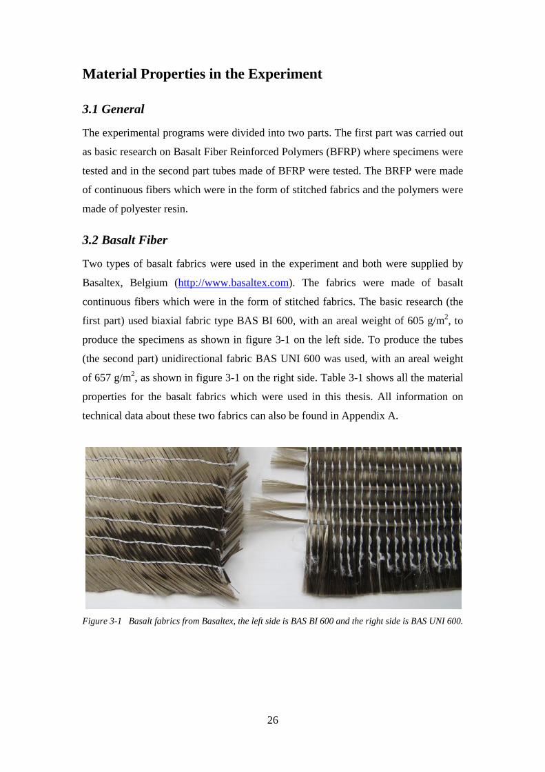
Two types of basalt fabrics were used in the experiment and both were supplied by
Basaltex, Belgium (http://www.basaltex.com). The fabrics were made of basalt
continuous fibers which were in the form of stitched fabrics. The basic research (the
first part) used biaxial fabric type BAS BI 600, with an areal weight of 605 g/m2, to
produce the specimens as shown in figure 3-1 on the left side. To produce the tubes
(the second part) unidirectional fabric BAS UNI 600 was used, with an areal weight
of 657 g/m2, as shown in figure 3-1 on the right side. Table 3-1 shows all the material
properties for the basalt fabrics which were used in this thesis. All information on
technical data about these two fabrics can also be found in Appendix A.
Figure 3-1 Basalt fabrics from Basaltex, the left side is BAS BI 600 and the right side is BAS UNI 600.
27
Table 3-1 Material properties of basalt fabrics.
Material Density Thickness Surface Tensile Tensile Elastic Type of basalt of fabrics weight strength strain modulus [g/cm3] [mm] [g/m2] [MPa] [%] [GPa]
BAS BI 600 2.67 0.5 605 2410 3.15 86.5
BAS UNI 600 2.67 0.65 657 2410 3.15 86.5
3.3 Polyester resin
Two types of polyester resin were used in the experiment and both were supplied by
Reichhold (http://www.reichhold.com). The experiment used two types of
manufacturing processes to create the BFRP in composite laminate; for that reason it
was not possible to use the same type of polyester resin. The Hand Lay-up process
used POLYLITE 440-M850 (standard polyester resin) and the Vacuum Infusion
process used POLYLITE 506-647 (designed for vacuum infusion processes). Table 3-
2 shows all the material properties for the polyester resins which were used in this
study. All information on the technical data about these two polyester resins from
Reichhold can also be found in Appendix B.
Table 3-2 Material properties of polyester resin.
Material Density Tensile Tensile Elastic type of resin strength strain modulus [g/cm3] [MPa] [%] [GPa]
POLYLITE 506-647 1.11 50 2.1 3.1
POLYLITE 440-M850 1.10 50 1.6 4.6
3.4 Summary
• Two types of basalt fabrics were used made of basalt continuous fibers which
were in the form of stitched fabrics.
• Two types of polyester resin were used, for the Hand Lay-up process and the
Vacuum Infusion process.
28
Experimental Program and Procedures, Part 1
4.1 General
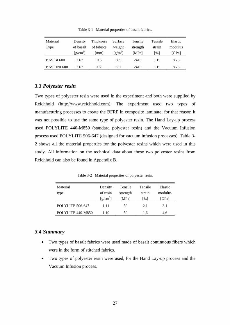
In the first part of the experiment two thin plates made of BFRP laminate were made
by using the Vacuum Infusion process. The plates were made in the structural
laboratory at Reykjavík University. The plats were cut down with a saw into
rectangular specimens. The specimens were tested for uniaxial tension, compression,
in-plane shear and pin bearing.
4.2 Fabrication Procedure of the Fiber plates
Two types of thin plates were made, using the same reinforcement biaxial fabric type
BAS BI 600 and the same matrix polyester resins POLYLITE 506-647. The plates
were made of six pieces of fabric where each fabric was 0.5 mm thick and covered
two layers with an areal weight of each layer 298.5 g/m2. The lamination sequences
for these two plates with twelve layers were:
Plate no.1 = [(±45°)3]S Plate no.2 = [0°/90°/±45°/0°/90°]S This symmetrical lamination sequence was selected to prevent problems of strain
coupling between the layers. Figure 4-1 illustrates, to the left, these six fabrics which
were placed on the mold in two different directions, i.e. 0° and 45°. First the fabrics
were placed in the mold and then the peel ply, distribution media and vacuum bag
were placed on in this order, as shown in figure 4-1 to the right. The peel ply was used
to prevent the distribution media from sticking to the laminate plates. The distribution
media was used to distribute the resin equally and easily around the plates. The
vacuum bag was sealed to the mold with sealant tape (color yellow) as shown in
figure 4-1 to the right.
Figure 4-1 Basalt fabrics type BAS BI 600 (to the left) and vacuum infusion process (to the right).
29
The vacuum pump was used to vacuum out the air from the system and checked for
leaking before the polyester resin was infused into the system. When the polyester
resin was infused through the fabrics, as shown in figure 4-2 to the left, the system
had attained a 90% vacuum. When the fabrics were saturated by polyester resin the
vacuum was reduced to 50% for four hours during which time the resin was to harden.
Figure 4-2 to the right shows the laminate plates after the vacuum infusion process
and the thickness of the plates measured 2.7mm (on average). The width and length of
plate no.1 ([(±45°)3]S) was 900 x 450 mm and the width and length of plate no.2
([0°/90°/±45°/0°/90°]S) was 450 x 450 mm.
Figure 4-2 The polyester resin was infused through the basalt fabrics (to the left). The laminate plates
completed after the vacuum infusion process (to the right).
4.2 Constituent Content Determination of the Fiber plates
The standard ASTM D3171“Constituent Content of Composite Materials” (ASTM
D3171, 2000) was used to ascertain the composite density, the weight and volume
ratio for the reinforcement and the matrix for each specimen. Method II in the
standard was used because the basalt fabric areal weight was known. Equation (4.1)
demonstrates how the specimen density (composite density) was found.
𝜌𝜌𝑐𝑐 =𝑚𝑚𝑡𝑡𝑠𝑠𝑠𝑠 𝑡𝑡𝑓𝑓 𝑡𝑡ℎ𝑒𝑒 𝑠𝑠𝑠𝑠𝑒𝑒𝑐𝑐𝑖𝑖𝑚𝑚𝑒𝑒𝑠𝑠𝑣𝑣𝑡𝑡𝑡𝑡𝑏𝑏𝑚𝑚𝑒𝑒 𝑡𝑡𝑓𝑓 𝑡𝑡ℎ𝑒𝑒 𝑠𝑠𝑠𝑠𝑒𝑒𝑐𝑐𝑖𝑖𝑚𝑚𝑒𝑒𝑠𝑠
(4.1)
30
The basalt fiber weight percent 𝑊𝑊𝑓𝑓 was calculated for all specimens, as expressed in
equation (4.2).
𝑊𝑊𝑓𝑓 = 100 ∗𝐴𝐴𝑓𝑓 ∗ 𝑁𝑁𝜌𝜌𝑐𝑐 ∗ ℎ
The basalt fiber volume percent 𝑉𝑉𝑓𝑓 was calculated for all specimens, as expressed in
equation (4.3).
𝑉𝑉𝑓𝑓 = 𝑊𝑊𝑓𝑓 ∗𝜌𝜌𝑐𝑐𝜌𝜌𝑓𝑓
The polyester resin weight percent 𝑊𝑊𝑚𝑚 was calculated for all specimens, as expressed
in equation (4.4).
𝑊𝑊𝑚𝑚 = 100 −𝑊𝑊𝑓𝑓
The polyester resin volume percent 𝑉𝑉𝑚𝑚 was calculated for all specimens, as expressed
in equation (4.5).
𝑉𝑉𝑚𝑚 = 𝑊𝑊𝑚𝑚 ∗𝜌𝜌𝑐𝑐𝜌𝜌𝑚𝑚
where: 𝐴𝐴𝑓𝑓 = 605 g/m2weight of basalt fabric BAS BI 600 (Appendix A)
𝑁𝑁 = 6 fabrics, number of fabrics in the specimen
ℎ = average 2.7 mm thickness of the specimen (Appendix C)
𝜌𝜌𝑓𝑓 = 2.67 g/cm3 density of the basalt fiber Basaltex (Appendix A)
𝜌𝜌𝑚𝑚 = 1.1 g/cm3density of the polyester resin POLYLITE 506-647 (Appendix B)
All measurements for the specimens, such as the mass, thickness and volume, can be
found in Appendix C.
(4.2)
(4.3)
(4.4)
(4.5)
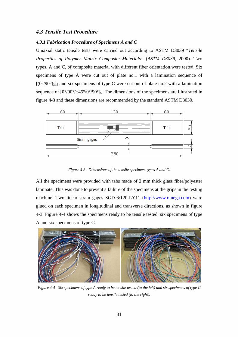
31
4.3 Tensile Test Procedure
4.3.1 Fabrication Procedure of Specimens A and C
Uniaxial static tensile tests were carried out according to ASTM D3039 “Tensile
Properties of Polymer Matrix Composite Materials” (ASTM D3039, 2000). Two
types, A and C, of composite material with different fiber orientation were tested. Six
specimens of type A were cut out of plate no.1 with a lamination sequence of
[(0°/90°)3]S and six specimens of type C were cut out of plate no.2 with a lamination
sequence of [0°/90°/±45°/0°/90°]S. The dimensions of the specimens are illustrated in
figure 4-3 and these dimensions are recommended by the standard ASTM D3039.
Figure 4-3 Dimensions of the tensile specimen, types A and C.
All the specimens were provided with tabs made of 2 mm thick glass fiber/polyester
laminate. This was done to prevent a failure of the specimens at the grips in the testing
machine. Two linear strain gages SGD-6/120-LY11 (http://www.omega.com) were
glued on each specimen in longitudinal and transverse directions, as shown in figure
4-3. Figure 4-4 shows the specimens ready to be tensile tested, six specimens of type
A and six specimens of type C.
Figure 4-4 Six specimens of type A ready to be tensile tested (to the left) and six specimens of type C
ready to be tensile tested (to the right).
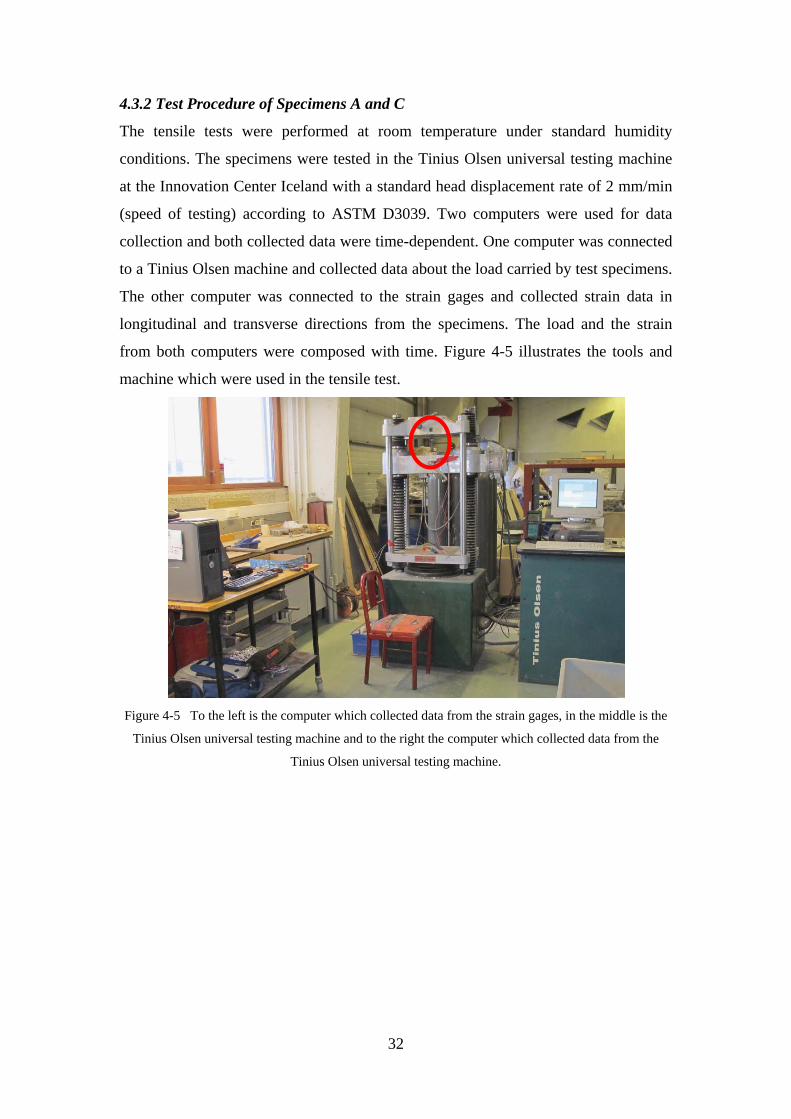
32
4.3.2 Test Procedure of Specimens A and C
The tensile tests were performed at room temperature under standard humidity
conditions. The specimens were tested in the Tinius Olsen universal testing machine
at the Innovation Center Iceland with a standard head displacement rate of 2 mm/min
(speed of testing) according to ASTM D3039. Two computers were used for data
collection and both collected data were time-dependent. One computer was connected
to a Tinius Olsen machine and collected data about the load carried by test specimens.
The other computer was connected to the strain gages and collected strain data in
longitudinal and transverse directions from the specimens. The load and the strain
from both computers were composed with time. Figure 4-5 illustrates the tools and
machine which were used in the tensile test.
Figure 4-5 To the left is the computer which collected data from the strain gages, in the middle is the
Tinius Olsen universal testing machine and to the right the computer which collected data from the
Tinius Olsen universal testing machine.
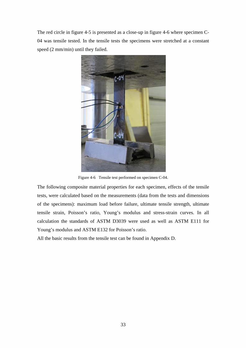
33
The red circle in figure 4-5 is presented as a close-up in figure 4-6 where specimen C-
04 was tensile tested. In the tensile tests the specimens were stretched at a constant
speed (2 mm/min) until they failed.
Figure 4-6 Tensile test performed on specimen C-04.
The following composite material properties for each specimen, effects of the tensile
tests, were calculated based on the measurements (data from the tests and dimensions
of the specimens): maximum load before failure, ultimate tensile strength, ultimate
tensile strain, Poisson’s ratio, Young’s modulus and stress-strain curves. In all
calculation the standards of ASTM D3039 were used as well as ASTM E111 for
Young’s modulus and ASTM E132 for Poisson’s ratio.
All the basic results from the tensile test can be found in Appendix D.
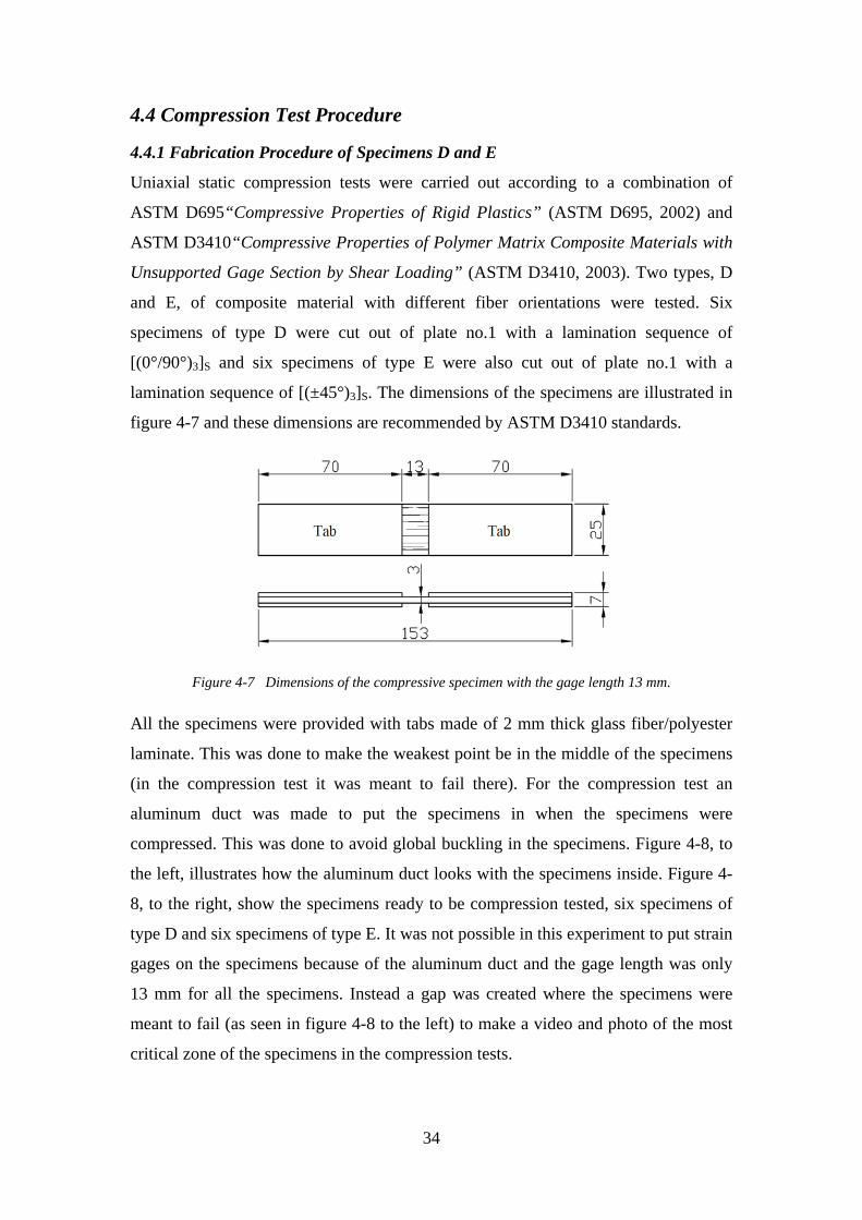
34
4.4 Compression Test Procedure
4.4.1 Fabrication Procedure of Specimens D and E
Uniaxial static compression tests were carried out according to a combination of
ASTM D695“Compressive Properties of Rigid Plastics” (ASTM D695, 2002) and
ASTM D3410“Compressive Properties of Polymer Matrix Composite Materials with
Unsupported Gage Section by Shear Loading” (ASTM D3410, 2003). Two types, D
and E, of composite material with different fiber orientations were tested. Six
specimens of type D were cut out of plate no.1 with a lamination sequence of
[(0°/90°)3]S and six specimens of type E were also cut out of plate no.1 with a
lamination sequence of [(±45°)3]S. The dimensions of the specimens are illustrated in
figure 4-7 and these dimensions are recommended by ASTM D3410 standards.
Figure 4-7 Dimensions of the compressive specimen with the gage length 13 mm.
All the specimens were provided with tabs made of 2 mm thick glass fiber/polyester
laminate. This was done to make the weakest point be in the middle of the specimens
(in the compression test it was meant to fail there). For the compression test an
aluminum duct was made to put the specimens in when the specimens were
compressed. This was done to avoid global buckling in the specimens. Figure 4-8, to
the left, illustrates how the aluminum duct looks with the specimens inside. Figure 4-
8, to the right, show the specimens ready to be compression tested, six specimens of
type D and six specimens of type E. It was not possible in this experiment to put strain
gages on the specimens because of the aluminum duct and the gage length was only
13 mm for all the specimens. Instead a gap was created where the specimens were
meant to fail (as seen in figure 4-8 to the left) to make a video and photo of the most
critical zone of the specimens in the compression tests.
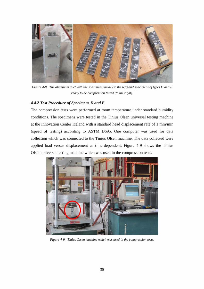
35
Figure 4-8 The aluminum duct with the specimens inside (to the left) and specimens of types D and E
ready to be compression tested (to the right).
4.4.2 Test Procedure of Specimens D and E
The compression tests were performed at room temperature under standard humidity
conditions. The specimens were tested in the Tinius Olsen universal testing machine
at the Innovation Center Iceland with a standard head displacement rate of 1 mm/min
(speed of testing) according to ASTM D695. One computer was used for data
collection which was connected to the Tinius Olsen machine. The data collected were
applied load versus displacement as time-dependent. Figure 4-9 shows the Tinius
Olsen universal testing machine which was used in the compression tests.
Figure 4-9 Tinius Olsen machine which was used in the compression tests.
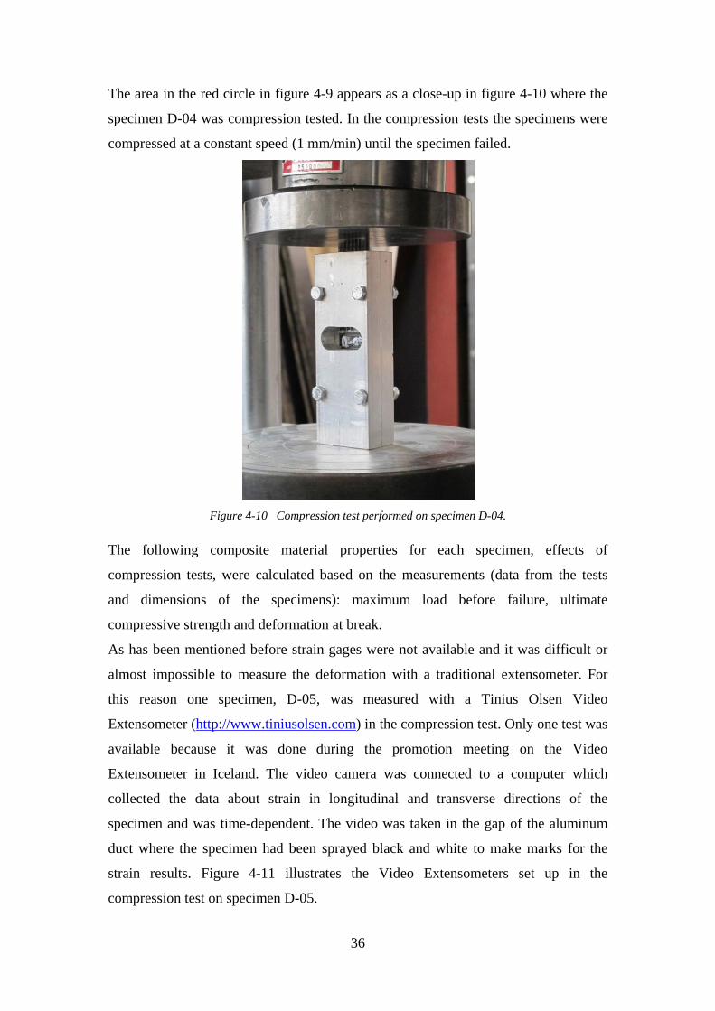
36
The area in the red circle in figure 4-9 appears as a close-up in figure 4-10 where the
specimen D-04 was compression tested. In the compression tests the specimens were
compressed at a constant speed (1 mm/min) until the specimen failed.
Figure 4-10 Compression test performed on specimen D-04.
The following composite material properties for each specimen, effects of
compression tests, were calculated based on the measurements (data from the tests
and dimensions of the specimens): maximum load before failure, ultimate
compressive strength and deformation at break.
As has been mentioned before strain gages were not available and it was difficult or
almost impossible to measure the deformation with a traditional extensometer. For
this reason one specimen, D-05, was measured with a Tinius Olsen Video
Extensometer (http://www.tiniusolsen.com) in the compression test. Only one test was
available because it was done during the promotion meeting on the Video
Extensometer in Iceland. The video camera was connected to a computer which
collected the data about strain in longitudinal and transverse directions of the
specimen and was time-dependent. The video was taken in the gap of the aluminum
duct where the specimen had been sprayed black and white to make marks for the
strain results. Figure 4-11 illustrates the Video Extensometers set up in the
compression test on specimen D-05.
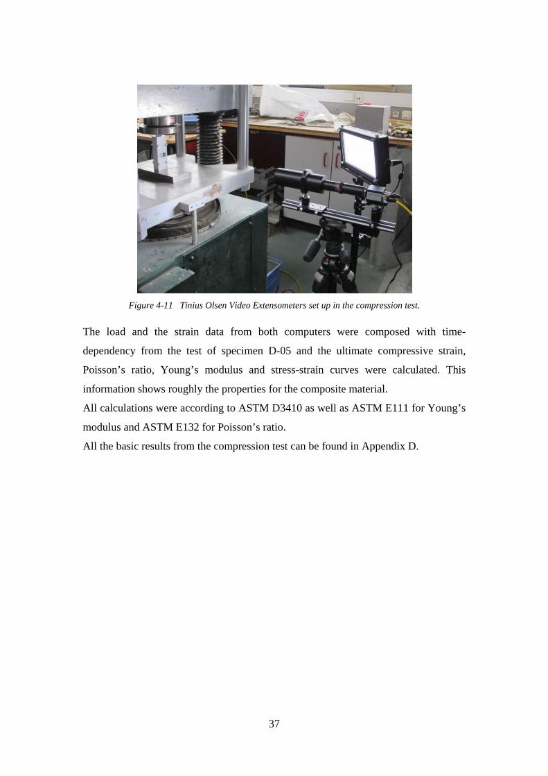
37
Figure 4-11 Tinius Olsen Video Extensometers set up in the compression test.
The load and the strain data from both computers were composed with time-
dependency from the test of specimen D-05 and the ultimate compressive strain,
Poisson’s ratio, Young’s modulus and stress-strain curves were calculated. This
information shows roughly the properties for the composite material.
All calculations were according to ASTM D3410 as well as ASTM E111 for Young’s
modulus and ASTM E132 for Poisson’s ratio.
All the basic results from the compression test can be found in Appendix D.
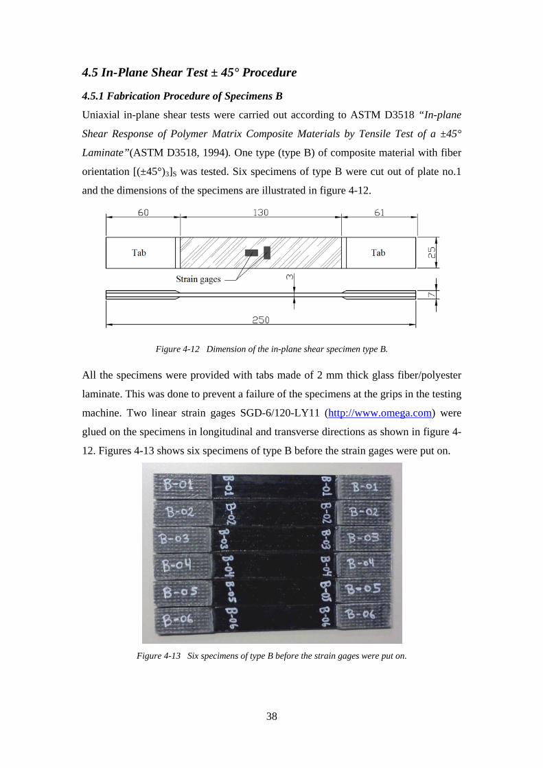
38
4.5 In-Plane Shear Test ± 45° Procedure
4.5.1 Fabrication Procedure of Specimens B
Uniaxial in-plane shear tests were carried out according to ASTM D3518 “In-plane
Shear Response of Polymer Matrix Composite Materials by Tensile Test of a ±45°
Laminate”(ASTM D3518, 1994). One type (type B) of composite material with fiber
orientation [(±45°)3]S was tested. Six specimens of type B were cut out of plate no.1
and the dimensions of the specimens are illustrated in figure 4-12.
Figure 4-12 Dimension of the in-plane shear specimen type B.
All the specimens were provided with tabs made of 2 mm thick glass fiber/polyester
laminate. This was done to prevent a failure of the specimens at the grips in the testing
machine. Two linear strain gages SGD-6/120-LY11 (http://www.omega.com) were
glued on the specimens in longitudinal and transverse directions as shown in figure 4-
12. Figures 4-13 shows six specimens of type B before the strain gages were put on.
Figure 4-13 Six specimens of type B before the strain gages were put on.
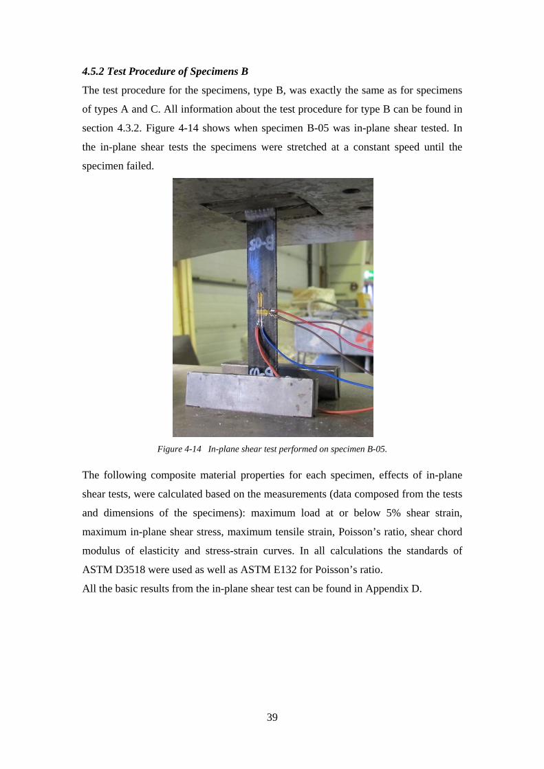
39
4.5.2 Test Procedure of Specimens B
The test procedure for the specimens, type B, was exactly the same as for specimens
of types A and C. All information about the test procedure for type B can be found in
section 4.3.2. Figure 4-14 shows when specimen B-05 was in-plane shear tested. In
the in-plane shear tests the specimens were stretched at a constant speed until the
specimen failed.
Figure 4-14 In-plane shear test performed on specimen B-05.
The following composite material properties for each specimen, effects of in-plane
shear tests, were calculated based on the measurements (data composed from the tests
and dimensions of the specimens): maximum load at or below 5% shear strain,
maximum in-plane shear stress, maximum tensile strain, Poisson’s ratio, shear chord
modulus of elasticity and stress-strain curves. In all calculations the standards of
ASTM D3518 were used as well as ASTM E132 for Poisson’s ratio.
All the basic results from the in-plane shear test can be found in Appendix D.
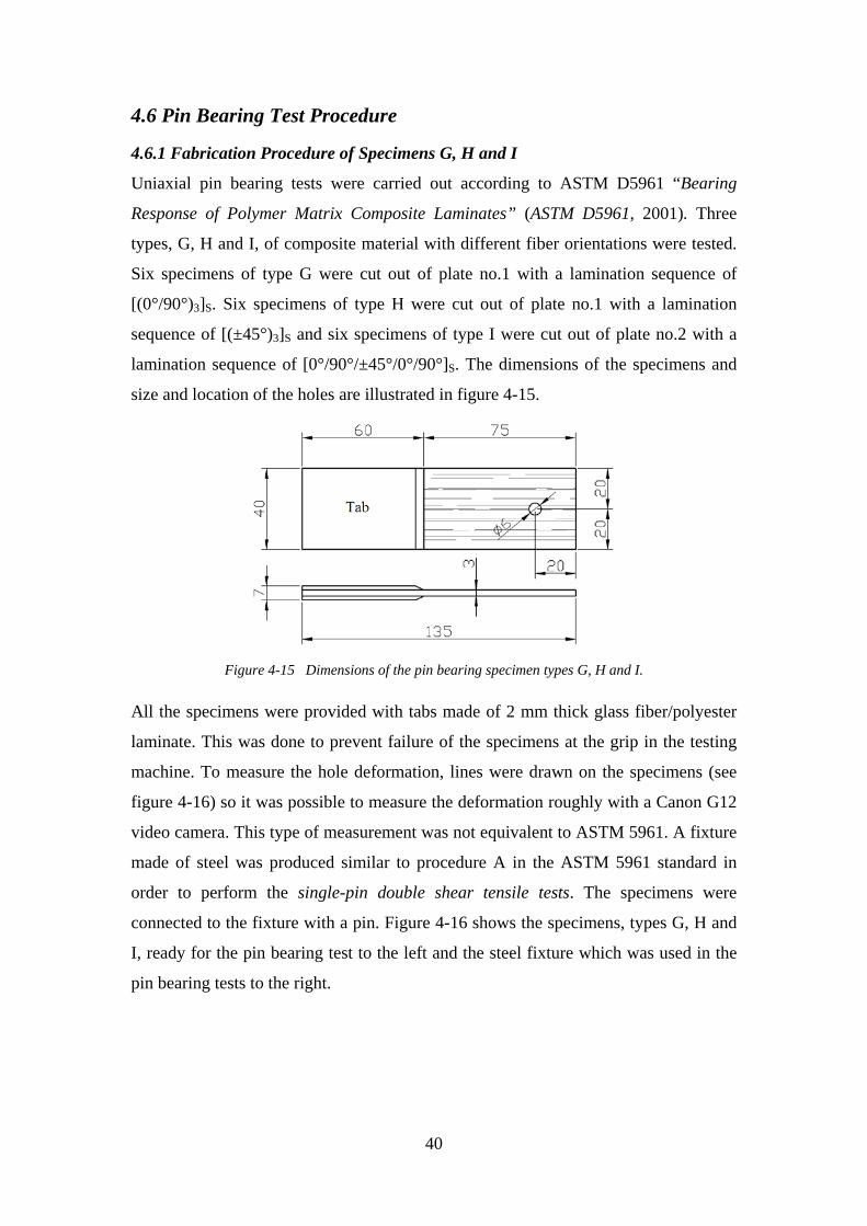
40
4.6 Pin Bearing Test Procedure
4.6.1 Fabrication Procedure of Specimens G, H and I
Uniaxial pin bearing tests were carried out according to ASTM D5961 “Bearing
Response of Polymer Matrix Composite Laminates” (ASTM D5961, 2001). Three
types, G, H and I, of composite material with different fiber orientations were tested.
Six specimens of type G were cut out of plate no.1 with a lamination sequence of
[(0°/90°)3]S. Six specimens of type H were cut out of plate no.1 with a lamination
sequence of [(±45°)3]S and six specimens of type I were cut out of plate no.2 with a
lamination sequence of [0°/90°/±45°/0°/90°]S. The dimensions of the specimens and
size and location of the holes are illustrated in figure 4-15.
Figure 4-15 Dimensions of the pin bearing specimen types G, H and I.
All the specimens were provided with tabs made of 2 mm thick glass fiber/polyester
laminate. This was done to prevent failure of the specimens at the grip in the testing
machine. To measure the hole deformation, lines were drawn on the specimens (see
figure 4-16) so it was possible to measure the deformation roughly with a Canon G12
video camera. This type of measurement was not equivalent to ASTM 5961. A fixture
made of steel was produced similar to procedure A in the ASTM 5961 standard in
order to perform the single-pin double shear tensile tests. The specimens were
connected to the fixture with a pin. Figure 4-16 shows the specimens, types G, H and
I, ready for the pin bearing test to the left and the steel fixture which was used in the
pin bearing tests to the right.
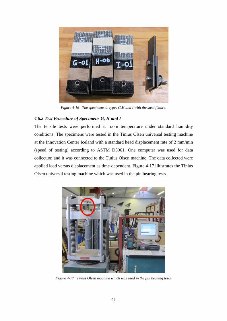
41
Figure 4-16 The specimens in types G,H and I with the steel fixture.
4.6.2 Test Procedure of Specimens G, H and I
The tensile tests were performed at room temperature under standard humidity
conditions. The specimens were tested in the Tinius Olsen universal testing machine
at the Innovation Center Iceland with a standard head displacement rate of 2 mm/min
(speed of testing) according to ASTM D5961. One computer was used for data
collection and it was connected to the Tinius Olsen machine. The data collected were
applied load versus displacement as time-dependent. Figure 4-17 illustrates the Tinius
Olsen universal testing machine which was used in the pin bearing tests.
Figure 4-17 Tinius Olsen machine which was used in the pin bearing tests.
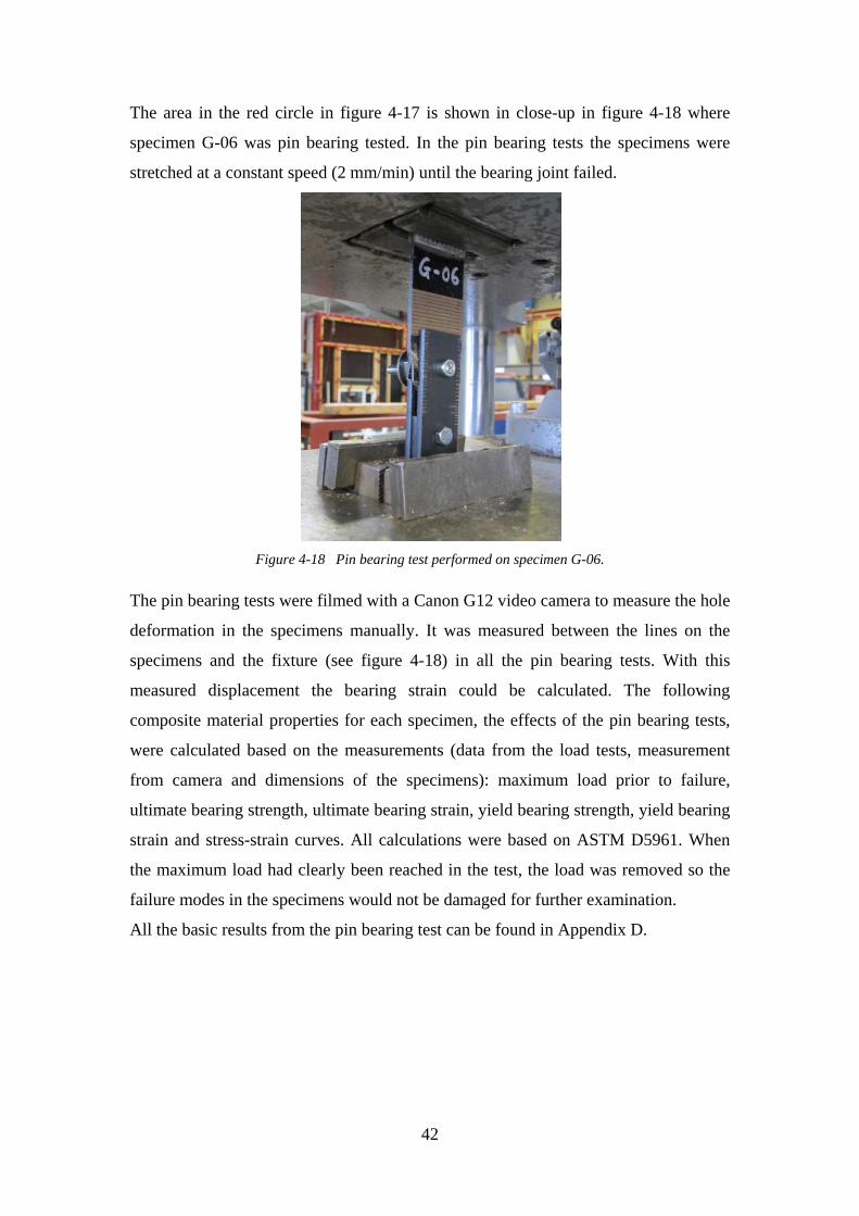
42
The area in the red circle in figure 4-17 is shown in close-up in figure 4-18 where
specimen G-06 was pin bearing tested. In the pin bearing tests the specimens were
stretched at a constant speed (2 mm/min) until the bearing joint failed.
Figure 4-18 Pin bearing test performed on specimen G-06.
The pin bearing tests were filmed with a Canon G12 video camera to measure the hole
deformation in the specimens manually. It was measured between the lines on the
specimens and the fixture (see figure 4-18) in all the pin bearing tests. With this
measured displacement the bearing strain could be calculated. The following
composite material properties for each specimen, the effects of the pin bearing tests,
were calculated based on the measurements (data from the load tests, measurement
from camera and dimensions of the specimens): maximum load prior to failure,
ultimate bearing strength, ultimate bearing strain, yield bearing strength, yield bearing
strain and stress-strain curves. All calculations were based on ASTM D5961. When
the maximum load had clearly been reached in the test, the load was removed so the
failure modes in the specimens would not be damaged for further examination.
All the basic results from the pin bearing test can be found in Appendix D.
43
4.7 Summary
• Composite laminate plates where made with a Vacuum Infusion process.
• The composite density, the weight and volume ratio for the reinforcement and
the matrix for each specimen were calculated.
• A tensile test was performed on twelve specimens, types A and C.
• A compression test was performed on twelve specimens, types D and E.
• An in-plane shear test was performed on six specimens, type B.
• A pin bearing test was performed on eighteen specimens, types G, H and I.
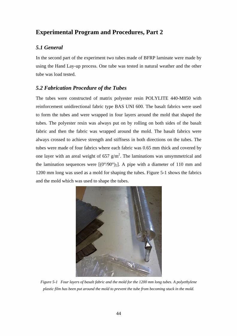
44
Experimental Program and Procedures, Part 2
5.1 General
In the second part of the experiment two tubes made of BFRP laminate were made by
using the Hand Lay-up process. One tube was tested in natural weather and the other
tube was load tested.
5.2 Fabrication Procedure of the Tubes
The tubes were constructed of matrix polyester resin POLYLITE 440-M850 with
reinforcement unidirectional fabric type BAS UNI 600. The basalt fabrics were used
to form the tubes and were wrapped in four layers around the mold that shaped the
tubes. The polyester resin was always put on by rolling on both sides of the basalt
fabric and then the fabric was wrapped around the mold. The basalt fabrics were
always crossed to achieve strength and stiffness in both directions on the tubes. The
tubes were made of four fabrics where each fabric was 0.65 mm thick and covered by
one layer with an areal weight of 657 g/m2. The laminations was unsymmetrical and
the lamination sequences were [(0°/90°)2]. A pipe with a diameter of 110 mm and
1200 mm long was used as a mold for shaping the tubes. Figure 5-1 shows the fabrics
and the mold which was used to shape the tubes.
Figure 5-1 Four layers of basalt fabric and the mold for the 1200 mm long tubes. A polyethylene
plastic film has been put around the mold to prevent the tube from becoming stuck in the mold.
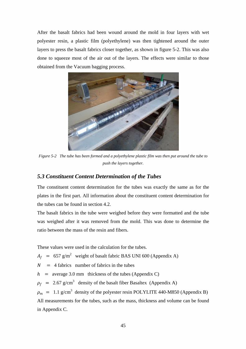
45
After the basalt fabrics had been wound around the mold in four layers with wet
polyester resin, a plastic film (polyethylene) was then tightened around the outer
layers to press the basalt fabrics closer together, as shown in figure 5-2. This was also
done to squeeze most of the air out of the layers. The effects were similar to those
obtained from the Vacuum bagging process.
Figure 5-2 The tube has been formed and a polyethylene plastic film was then put around the tube to
push the layers together.
5.3 Constituent Content Determination of the Tubes
The constituent content determination for the tubes was exactly the same as for the
plates in the first part. All information about the constituent content determination for
the tubes can be found in section 4.2.
The basalt fabrics in the tube were weighed before they were formatted and the tube
was weighed after it was removed from the mold. This was done to determine the
ratio between the mass of the resin and fibers.
These values were used in the calculation for the tubes.
𝐴𝐴𝑓𝑓 = 657 g/m2 weight of basalt fabric BAS UNI 600 (Appendix A)
𝑁𝑁 = 4 fabrics number of fabrics in the tubes
ℎ = average 3.0 mm thickness of the tubes (Appendix C)
𝜌𝜌𝑓𝑓 = 2.67 g/cm3 density of the basalt fiber Basaltex (Appendix A)
𝜌𝜌𝑚𝑚 = 1.1 g/cm3 density of the polyester resin POLYLITE 440-M850 (Appendix B)
All measurements for the tubes, such as the mass, thickness and volume can be found
in Appendix C.
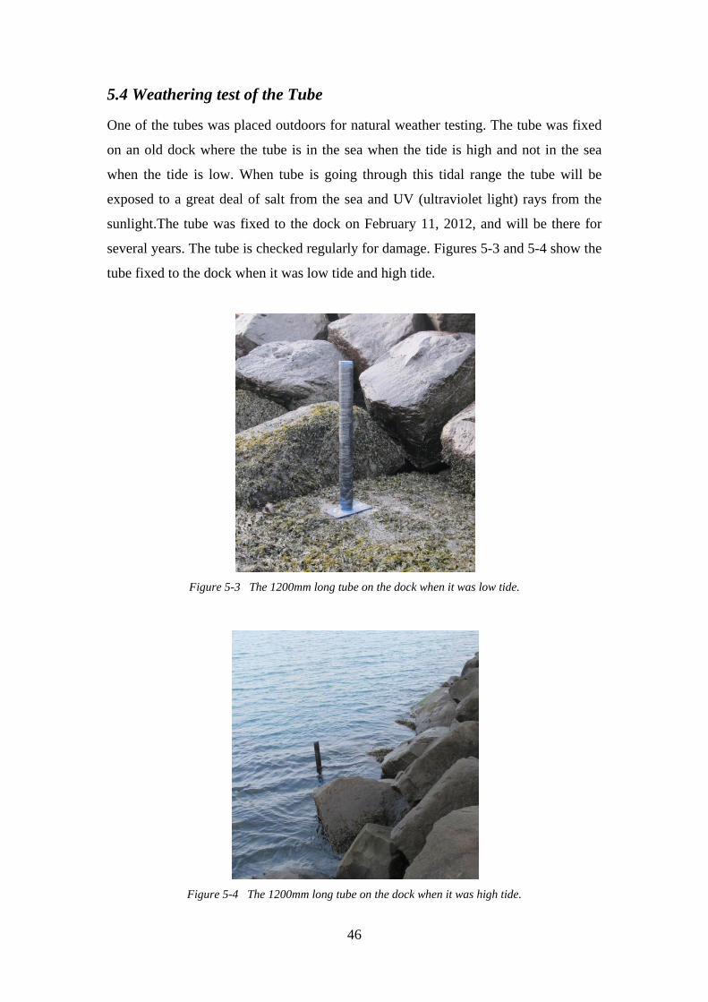
46
5.4 Weathering test of the Tube
One of the tubes was placed outdoors for natural weather testing. The tube was fixed
on an old dock where the tube is in the sea when the tide is high and not in the sea
when the tide is low. When tube is going through this tidal range the tube will be
exposed to a great deal of salt from the sea and UV (ultraviolet light) rays from the
sunlight.The tube was fixed to the dock on February 11, 2012, and will be there for
several years. The tube is checked regularly for damage. Figures 5-3 and 5-4 show the
tube fixed to the dock when it was low tide and high tide.
Figure 5-3 The 1200mm long tube on the dock when it was low tide.
Figure 5-4 The 1200mm long tube on the dock when it was high tide.
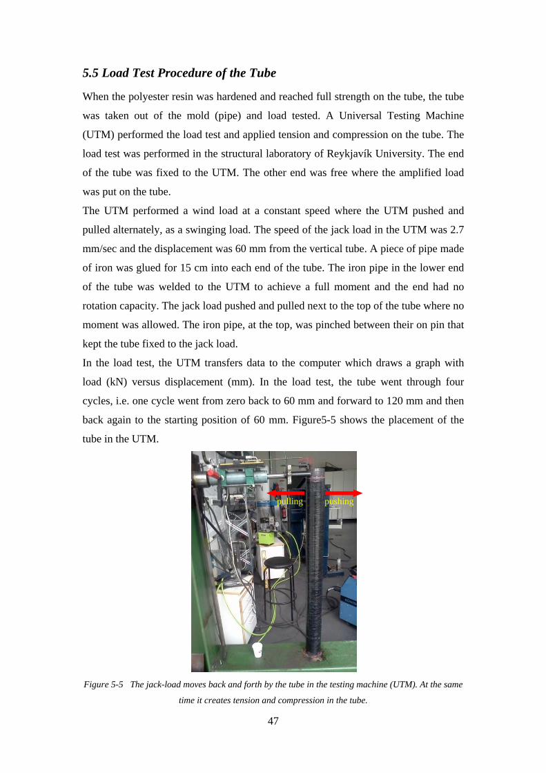
47
5.5 Load Test Procedure of the Tube
When the polyester resin was hardened and reached full strength on the tube, the tube
was taken out of the mold (pipe) and load tested. A Universal Testing Machine
(UTM) performed the load test and applied tension and compression on the tube. The
load test was performed in the structural laboratory of Reykjavík University. The end
of the tube was fixed to the UTM. The other end was free where the amplified load
was put on the tube.
The UTM performed a wind load at a constant speed where the UTM pushed and
pulled alternately, as a swinging load. The speed of the jack load in the UTM was 2.7
mm/sec and the displacement was 60 mm from the vertical tube. A piece of pipe made
of iron was glued for 15 cm into each end of the tube. The iron pipe in the lower end
of the tube was welded to the UTM to achieve a full moment and the end had no
rotation capacity. The jack load pushed and pulled next to the top of the tube where no
moment was allowed. The iron pipe, at the top, was pinched between their on pin that
kept the tube fixed to the jack load.
In the load test, the UTM transfers data to the computer which draws a graph with
load (kN) versus displacement (mm). In the load test, the tube went through four
cycles, i.e. one cycle went from zero back to 60 mm and forward to 120 mm and then
back again to the starting position of 60 mm. Figure5-5 shows the placement of the
tube in the UTM.
Figure 5-5 The jack-load moves back and forth by the tube in the testing machine (UTM). At the same
time it creates tension and compression in the tube.
pulling pushing

48
5.6 Summary
• Two tubes were made of BFRP laminate by using the Hand Lay-up.
• One of the tubes was placed outdoors for natural weather testing.
• The second tube was load tested, where the UTM pushed and pulled
alternately, as a swinging load.
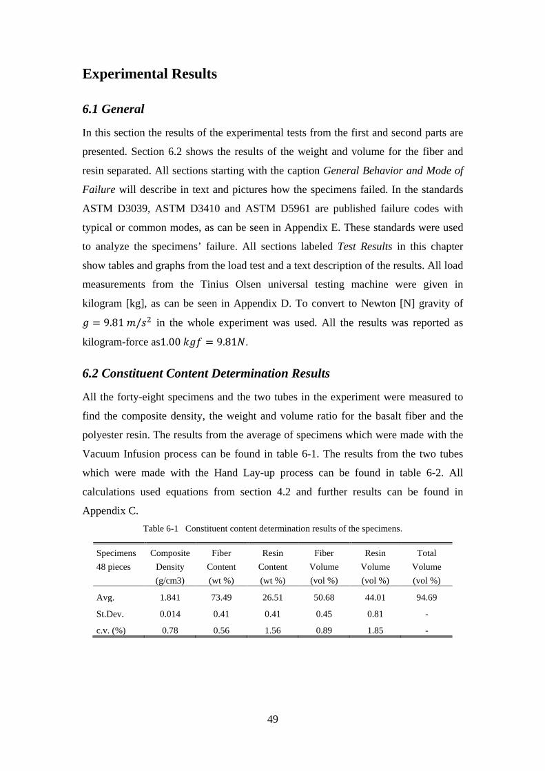
49
Experimental Results
6.1 General
In this section the results of the experimental tests from the first and second parts are
presented. Section 6.2 shows the results of the weight and volume for the fiber and
resin separated. All sections starting with the caption General Behavior and Mode of
Failure will describe in text and pictures how the specimens failed. In the standards
ASTM D3039, ASTM D3410 and ASTM D5961 are published failure codes with
typical or common modes, as can be seen in Appendix E. These standards were used
to analyze the specimens’ failure. All sections labeled Test Results in this chapter
show tables and graphs from the load test and a text description of the results. All load
measurements from the Tinius Olsen universal testing machine were given in
kilogram [kg], as can be seen in Appendix D. To convert to Newton [N] gravity of
𝑔𝑔 = 9.81 𝑚𝑚/𝑠𝑠2 in the whole experiment was used. All the results was reported as
kilogram-force as1.00 𝑘𝑘𝑔𝑔𝑓𝑓 = 9.81𝑁𝑁.
6.2 Constituent Content Determination Results
All the forty-eight specimens and the two tubes in the experiment were measured to
find the composite density, the weight and volume ratio for the basalt fiber and the
polyester resin. The results from the average of specimens which were made with the
Vacuum Infusion process can be found in table 6-1. The results from the two tubes
which were made with the Hand Lay-up process can be found in table 6-2. All
calculations used equations from section 4.2 and further results can be found in
Appendix C. Table 6-1 Constituent content determination results of the specimens.
Specimens Composite Fiber Resin Fiber Resin Total 48 pieces Density Content Content Volume Volume Volume (g/cm3) (wt %) (wt %) (vol %) (vol %) (vol %)
Avg. 1.841 73.49 26.51 50.68 44.01 94.69
St.Dev. 0.014 0.41 0.41 0.45 0.81 -
c.v. (%) 0.78 0.56 1.56 0.89 1.85 -
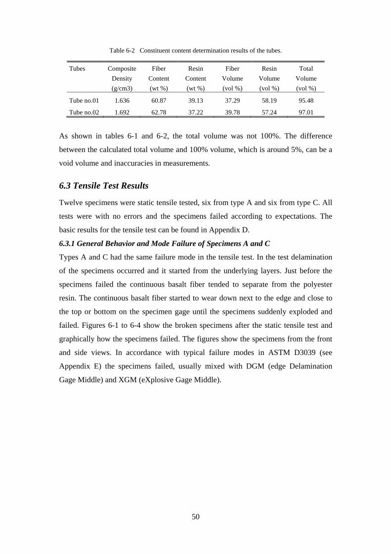
50
Table 6-2 Constituent content determination results of the tubes.
Tubes Composite Fiber Resin Fiber Resin Total
Density Content Content Volume Volume Volume
(g/cm3) (wt %) (wt %) (vol %) (vol %) (vol %)
Tube no.01 1.636 60.87 39.13 37.29 58.19 95.48
Tube no.02 1.692 62.78 37.22 39.78 57.24 97.01
As shown in tables 6-1 and 6-2, the total volume was not 100%. The difference
between the calculated total volume and 100% volume, which is around 5%, can be a
void volume and inaccuracies in measurements.
6.3 Tensile Test Results
Twelve specimens were static tensile tested, six from type A and six from type C. All
tests were with no errors and the specimens failed according to expectations. The
basic results for the tensile test can be found in Appendix D.
6.3.1 General Behavior and Mode Failure of Specimens A and C
Types A and C had the same failure mode in the tensile test. In the test delamination
of the specimens occurred and it started from the underlying layers. Just before the
specimens failed the continuous basalt fiber tended to separate from the polyester
resin. The continuous basalt fiber started to wear down next to the edge and close to
the top or bottom on the specimen gage until the specimens suddenly exploded and
failed. Figures 6-1 to 6-4 show the broken specimens after the static tensile test and
graphically how the specimens failed. The figures show the specimens from the front
and side views. In accordance with typical failure modes in ASTM D3039 (see
Appendix E) the specimens failed, usually mixed with DGM (edge Delamination
Gage Middle) and XGM (eXplosive Gage Middle).
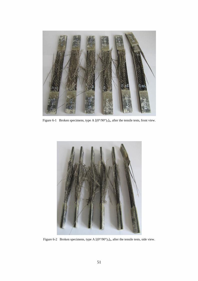
51
Figure 6-1 Broken specimens, type A [(0°/90°)3]S, after the tensile tests, front view.
Figure 6-2 Broken specimens, type A [(0°/90°)3]S, after the tensile tests, side view.
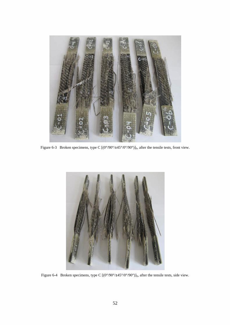
52
Figure 6-3 Broken specimens, type C [(0°/90°/±45°/0°/90°)]S, after the tensile tests, front view.
Figure 6-4 Broken specimens, type C [(0°/90°/±45°/0°/90°)]S, after the tensile tests, side view.
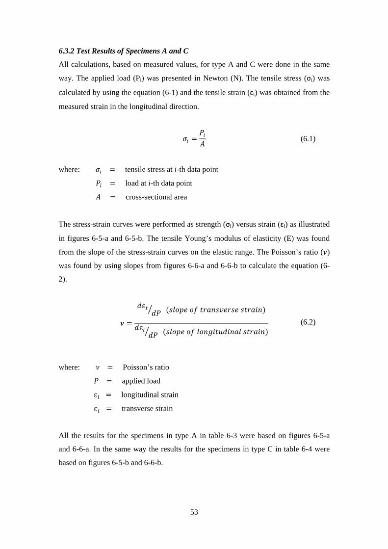
53
6.3.2 Test Results of Specimens A and C
All calculations, based on measured values, for type A and C were done in the same
way. The applied load (Pi) was presented in Newton (N). The tensile stress (σi) was
calculated by using the equation (6-1) and the tensile strain (ɛi) was obtained from the
measured strain in the longitudinal direction.
𝜎𝜎𝑖𝑖 =𝑃𝑃𝑖𝑖𝐴𝐴
where: 𝜎𝜎𝑖𝑖 = tensile stress at i-th data point
𝑃𝑃𝑖𝑖 = load at i-th data point
𝐴𝐴 = cross-sectional area
The stress-strain curves were performed as strength (σi) versus strain (ɛi) as illustrated
in figures 6-5-a and 6-5-b. The tensile Young’s modulus of elasticity (E) was found
from the slope of the stress-strain curves on the elastic range. The Poisson’s ratio (𝜈𝜈)
was found by using slopes from figures 6-6-a and 6-6-b to calculate the equation (6-
2).
𝜈𝜈 =
𝑑𝑑ɛ𝑡𝑡𝑑𝑑𝑃𝑃� (𝑠𝑠𝑡𝑡𝑡𝑡𝑠𝑠𝑒𝑒 𝑡𝑡𝑓𝑓 𝑡𝑡𝑏𝑏𝑡𝑡𝑠𝑠𝑠𝑠𝑣𝑣𝑒𝑒𝑏𝑏𝑠𝑠𝑒𝑒 𝑠𝑠𝑡𝑡𝑏𝑏𝑡𝑡𝑖𝑖𝑠𝑠)
𝑑𝑑ɛ𝑡𝑡𝑑𝑑𝑃𝑃� (𝑠𝑠𝑡𝑡𝑡𝑡𝑠𝑠𝑒𝑒 𝑡𝑡𝑓𝑓 𝑡𝑡𝑡𝑡𝑠𝑠𝑔𝑔𝑖𝑖𝑡𝑡𝑏𝑏𝑑𝑑𝑖𝑖𝑠𝑠𝑡𝑡𝑡𝑡 𝑠𝑠𝑡𝑡𝑏𝑏𝑡𝑡𝑖𝑖𝑠𝑠)
where: 𝜈𝜈 = Poisson’s ratio
𝑃𝑃 = applied load
ɛ𝑡𝑡 = longitudinal strain
ɛ𝑡𝑡 = transverse strain
All the results for the specimens in type A in table 6-3 were based on figures 6-5-a
and 6-6-a. In the same way the results for the specimens in type C in table 6-4 were
based on figures 6-5-b and 6-6-b.
(6.2)
(6.1)
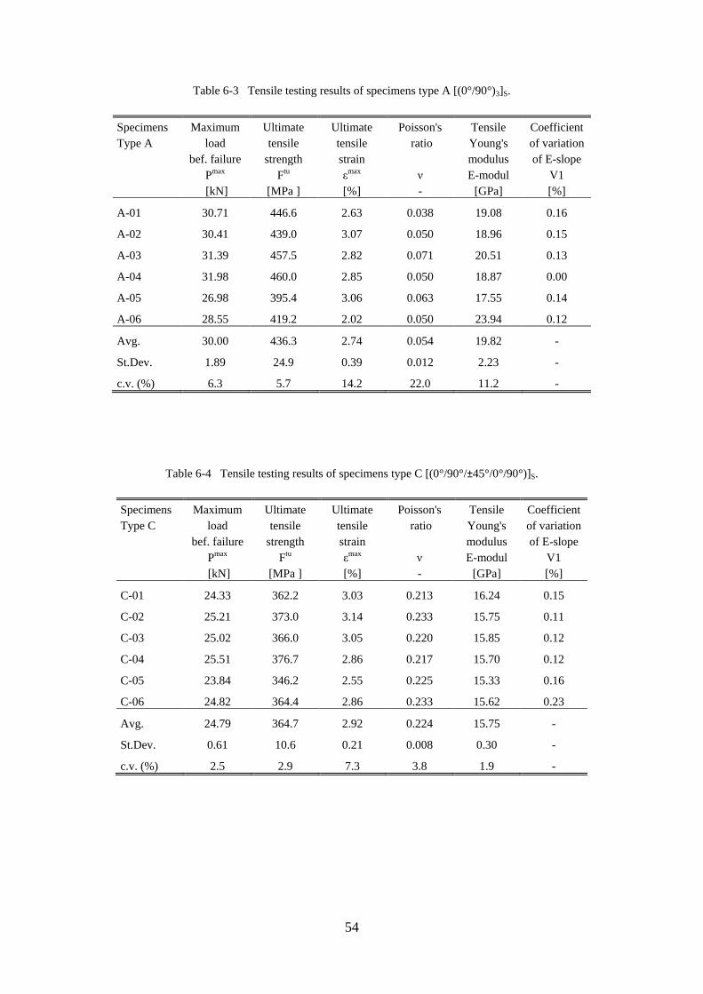
54
Table 6-3 Tensile testing results of specimens type A [(0°/90°)3]S.
Specimens Maximum Ultimate Ultimate Poisson's Tensile Coefficient Type A load tensile tensile ratio Young's of variation
bef. failure strength strain
modulus of E-slope
Pmax Ftu εmax ν E-modul V1
[kN] [MPa ] [%] - [GPa] [%]
A-01 30.71 446.6 2.63 0.038 19.08 0.16
A-02 30.41 439.0 3.07 0.050 18.96 0.15
A-03 31.39 457.5 2.82 0.071 20.51 0.13
A-04 31.98 460.0 2.85 0.050 18.87 0.00
A-05 26.98 395.4 3.06 0.063 17.55 0.14
A-06 28.55 419.2 2.02 0.050 23.94 0.12
Avg. 30.00 436.3 2.74 0.054 19.82 -
St.Dev. 1.89 24.9 0.39 0.012 2.23 -
c.v. (%) 6.3 5.7 14.2 22.0 11.2 -
Table 6-4 Tensile testing results of specimens type C [(0°/90°/±45°/0°/90°)]S.
Specimens Maximum Ultimate Ultimate Poisson's Tensile Coefficient Type C load tensile tensile ratio Young's of variation
bef. failure strength strain
modulus of E-slope
Pmax Ftu εmax ν E-modul V1
[kN] [MPa ] [%] - [GPa] [%]
C-01 24.33 362.2 3.03 0.213 16.24 0.15
C-02 25.21 373.0 3.14 0.233 15.75 0.11
C-03 25.02 366.0 3.05 0.220 15.85 0.12
C-04 25.51 376.7 2.86 0.217 15.70 0.12
C-05 23.84 346.2 2.55 0.225 15.33 0.16
C-06 24.82 364.4 2.86 0.233 15.62 0.23
Avg. 24.79 364.7 2.92 0.224 15.75 -
St.Dev. 0.61 10.6 0.21 0.008 0.30 -
c.v. (%) 2.5 2.9 7.3 3.8 1.9 -
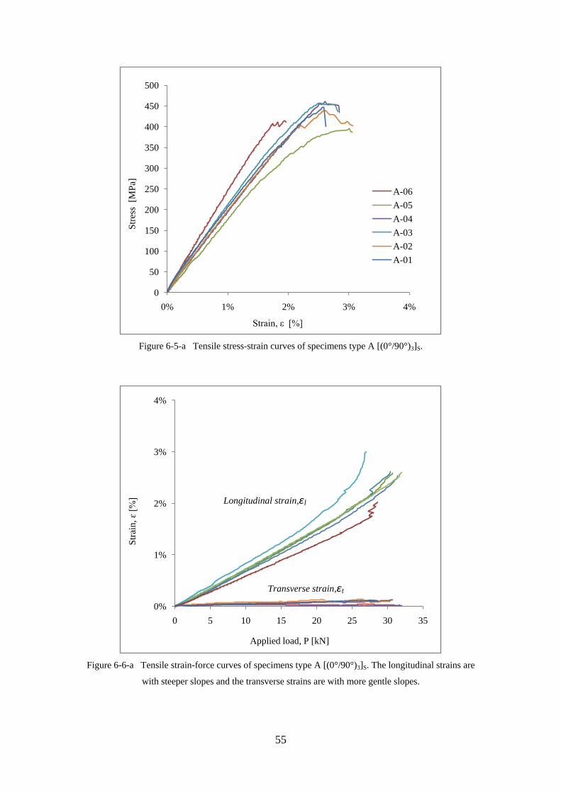
55
Figure 6-5-a Tensile stress-strain curves of specimens type A [(0°/90°)3]S.
Figure 6-6-a Tensile strain-force curves of specimens type A [(0°/90°)3]S. The longitudinal strains are
with steeper slopes and the transverse strains are with more gentle slopes.
0
50
100
150
200
250
300
350
400
450
500
0% 1% 2% 3% 4%
Stre
ss [
MPa
]
Strain, ε [%]
A-06A-05A-04A-03A-02A-01
0%
1%
2%
3%
4%
0 5 10 15 20 25 30 35
Stra
in, ɛ
[%]
Applied load, P [kN]
Transverse strain,ɛt
Longitudinal strain,ɛl
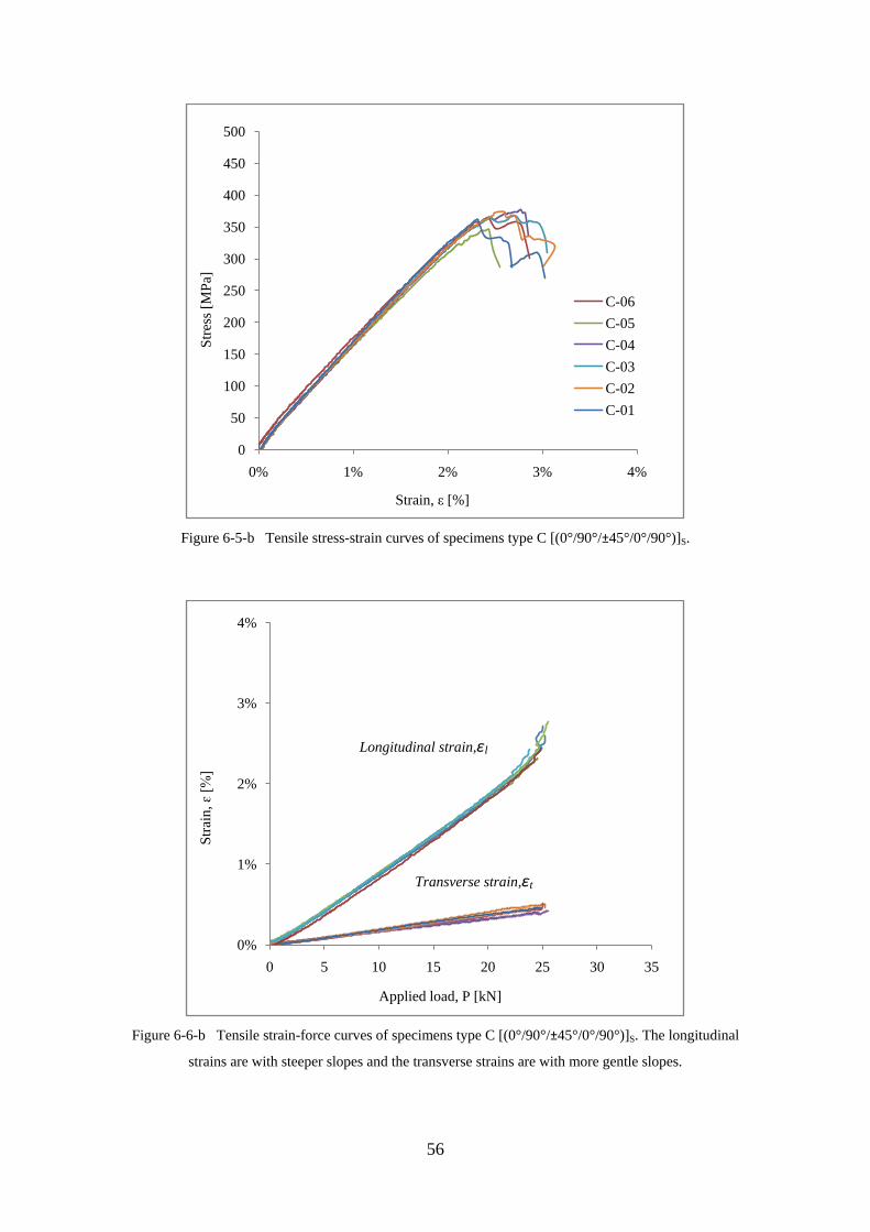
56
Figure 6-5-b Tensile stress-strain curves of specimens type C [(0°/90°/±45°/0°/90°)]S.
Figure 6-6-b Tensile strain-force curves of specimens type C [(0°/90°/±45°/0°/90°)]S. The longitudinal
strains are with steeper slopes and the transverse strains are with more gentle slopes.
0
50
100
150
200
250
300
350
400
450
500
0% 1% 2% 3% 4%
Stre
ss [M
Pa]
Strain, ε [%]
C-06C-05C-04C-03C-02C-01
0%
1%
2%
3%
4%
0 5 10 15 20 25 30 35
Stra
in, ɛ
[%]
Applied load, P [kN]
Longitudinal strain,ɛl
Transverse strain,ɛt
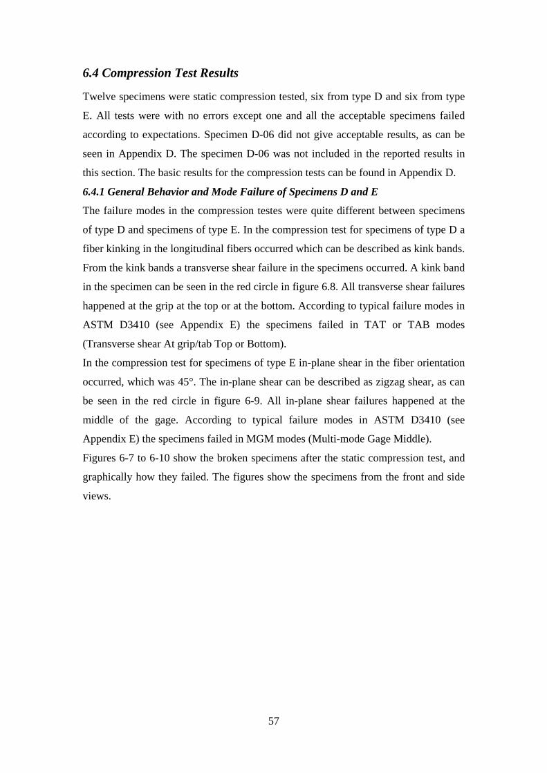
57
6.4 Compression Test Results
Twelve specimens were static compression tested, six from type D and six from type
E. All tests were with no errors except one and all the acceptable specimens failed
according to expectations. Specimen D-06 did not give acceptable results, as can be
seen in Appendix D. The specimen D-06 was not included in the reported results in
this section. The basic results for the compression tests can be found in Appendix D.
6.4.1 General Behavior and Mode Failure of Specimens D and E
The failure modes in the compression testes were quite different between specimens
of type D and specimens of type E. In the compression test for specimens of type D a
fiber kinking in the longitudinal fibers occurred which can be described as kink bands.
From the kink bands a transverse shear failure in the specimens occurred. A kink band
in the specimen can be seen in the red circle in figure 6.8. All transverse shear failures
happened at the grip at the top or at the bottom. According to typical failure modes in
ASTM D3410 (see Appendix E) the specimens failed in TAT or TAB modes
(Transverse shear At grip/tab Top or Bottom).
In the compression test for specimens of type E in-plane shear in the fiber orientation
occurred, which was 45°. The in-plane shear can be described as zigzag shear, as can
be seen in the red circle in figure 6-9. All in-plane shear failures happened at the
middle of the gage. According to typical failure modes in ASTM D3410 (see
Appendix E) the specimens failed in MGM modes (Multi-mode Gage Middle).
Figures 6-7 to 6-10 show the broken specimens after the static compression test, and
graphically how they failed. The figures show the specimens from the front and side
views.
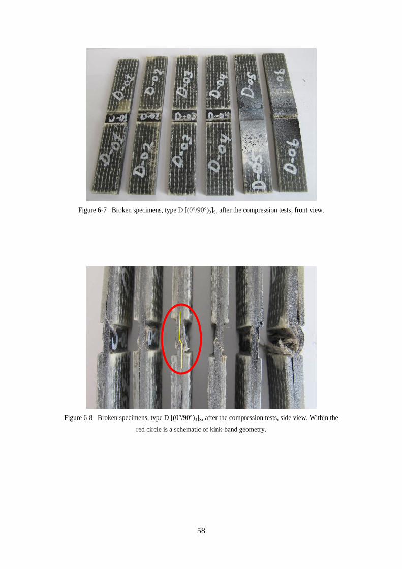
58
Figure 6-7 Broken specimens, type D [(0°/90°)3]S, after the compression tests, front view.
Figure 6-8 Broken specimens, type D [(0°/90°)3]S, after the compression tests, side view. Within the
red circle is a schematic of kink-band geometry.
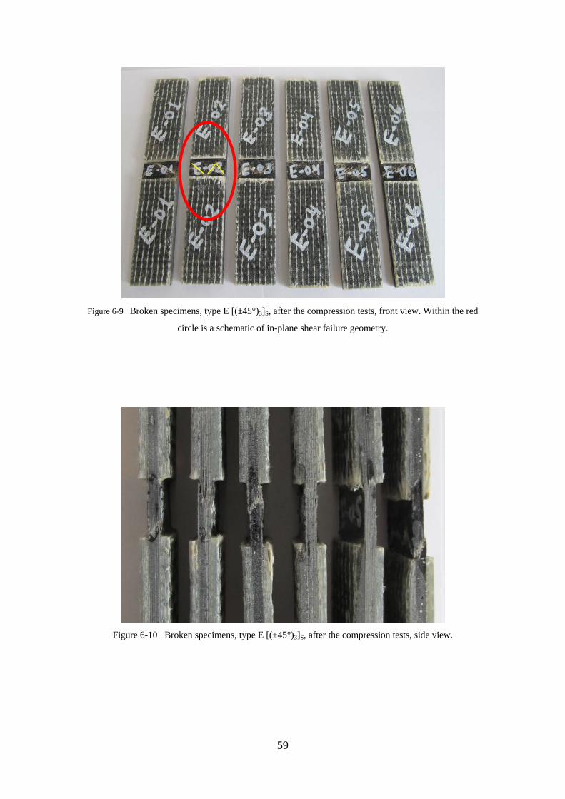
59
Figure 6-9 Broken specimens, type E [(±45°)3]S, after the compression tests, front view. Within the red
circle is a schematic of in-plane shear failure geometry.
Figure 6-10 Broken specimens, type E [(±45°)3]S, after the compression tests, side view.
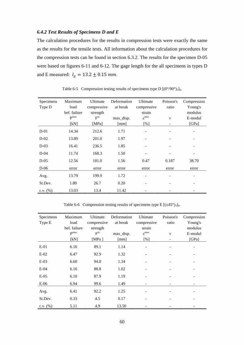
60
6.4.2 Test Results of Specimens D and E
The calculation procedures for the results in compression tests were exactly the same
as the results for the tensile tests. All information about the calculation procedures for
the compression tests can be found in section 6.3.2. The results for the specimen D-05
were based on figures 6-11 and 6-12. The gage length for the all specimens in types D
and E measured: 𝑡𝑡𝑔𝑔 = 13.2 ± 0.15 𝑚𝑚𝑚𝑚.
Table 6-5 Compression testing results of specimens type D [(0°/90°)3]S.
Specimens Maximum Ultimate Deformation Ultimate Poisson's Compression Type D load compressive at break compressive ratio Young's
bef. failure strength
strain
modulus
Pmax Ftu max_disp. εmax ν E-modul
[kN] [MPa] [mm] [%] - [GPa]
D-01 14.34 212.6 1.71 - - -
D-02 13.89 201.0 1.97 - - -
D-03 16.41 236.5 1.85 - - -
D-04 11.74 168.3 1.50 - - -
D-05 12.56 181.0 1.56 0.47 0.187 38.70
D-06 error error error error error error
Avg. 13.79 199.9 1.72 - - -
St.Dev. 1.80 26.7 0.20 - - -
c.v. (%) 13.03 13.4 11.42 - - -
Table 6-6 Compression testing results of specimens type E [(±45°)3]S.
Specimens Maximum Ultimate Deformation Ultimate Poisson's Compression Type E load compressive at break compressive ratio Young's
bef. failure strength
strain
modulus
Pmax Ftu max_disp. εmax ν E-modul
[kN] [MPa ] [mm] [%] - [GPa]
E-01 6.16 89.1 1.14 - - -
E-02 6.47 92.9 1.32 - - -
E-03 6.60 94.8 1.34 - - -
E-04 6.16 88.8 1.02 - - -
E-05 6.10 87.9 1.19 - - -
E-06 6.94 99.6 1.49 - - -
Avg. 6.41 92.2 1.25 - - -
St.Dev. 0.33 4.5 0.17 - - -
c.v. (%) 5.11 4.9 13.50 - - -
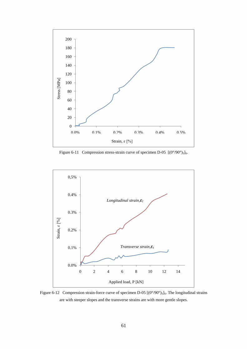
61
Figure 6-11 Compression stress-strain curve of specimen D-05 [(0°/90°)3]S.
Figure 6-12 Compression strain-force curve of specimen D-05 [(0°/90°)3]S. The longitudinal strains
are with steeper slopes and the transverse strains are with more gentle slopes.
0
20
40
60
80
100
120
140
160
180
200
0,0% 0,1% 0,2% 0,3% 0,4% 0,5%
Stre
ss [M
Pa]
Strain, ɛ [%]
0,0%
0,1%
0,2%
0,3%
0,4%
0,5%
0 2 4 6 8 10 12 14
Stra
in, ɛ
[%]
Applied load, P [kN]
Longitudinal strain,ɛl
Transverse strain,ɛt
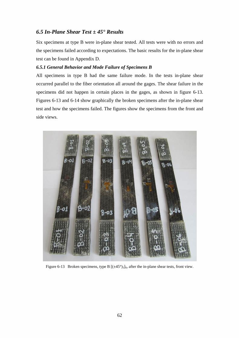
62
6.5 In-Plane Shear Test ± 45° Results
Six specimens at type B were in-plane shear tested. All tests were with no errors and
the specimens failed according to expectations. The basic results for the in-plane shear
test can be found in Appendix D.
6.5.1 General Behavior and Mode Failure of Specimens B
All specimens in type B had the same failure mode. In the tests in-plane shear
occurred parallel to the fiber orientation all around the gages. The shear failure in the
specimens did not happen in certain places in the gages, as shown in figure 6-13.
Figures 6-13 and 6-14 show graphically the broken specimens after the in-plane shear
test and how the specimens failed. The figures show the specimens from the front and
side views.
Figure 6-13 Broken specimens, type B [(±45°)3]S, after the in-plane shear tests, front view.
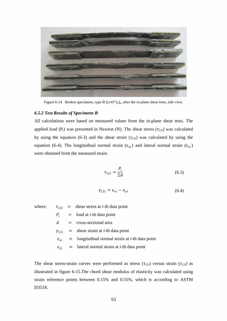
63
Figure 6-14 Broken specimens, type B [(±45°)3]S, after the in-plane shear tests, side view.
6.5.2 Test Results of Specimens B
All calculations were based on measured values from the in-plane shear tests. The
applied load (Pi) was presented in Newton (N). The shear stress (τ12i) was calculated
by using the equation (6-3) and the shear strain (γ12i) was calculated by using the
equation (6-4). The longitudinal normal strain (ɛ𝑥𝑥𝑖𝑖 ) and lateral normal strain (ɛ𝑥𝑥𝑖𝑖 )
were obtained from the measured strain.
𝜏𝜏12𝑖𝑖 =𝑃𝑃𝑖𝑖2𝐴𝐴
𝛾𝛾12𝑖𝑖 = ɛ𝑥𝑥𝑖𝑖 − ɛ𝑦𝑦𝑖𝑖
where: 𝜏𝜏12𝑖𝑖 = shear stress at i-th data point
𝑃𝑃𝑖𝑖 = load at i-th data point
𝐴𝐴 = cross-sectional area
𝛾𝛾12𝑖𝑖 = shear strain at i-th data point
ɛ𝑥𝑥𝑖𝑖 = longitudinal normal strain at i-th data point
ɛ𝑦𝑦𝑖𝑖 = lateral normal strain at i-th data point
The shear stress-strain curves were performed as stress (τ12i) versus strain (γ12i) as
illustrated in figure 6-15.The chord shear modulus of elasticity was calculated using
strain reference points between 0.15% and 0.55%, which is according to ASTM
D3518.
(6.3)
(6.4)
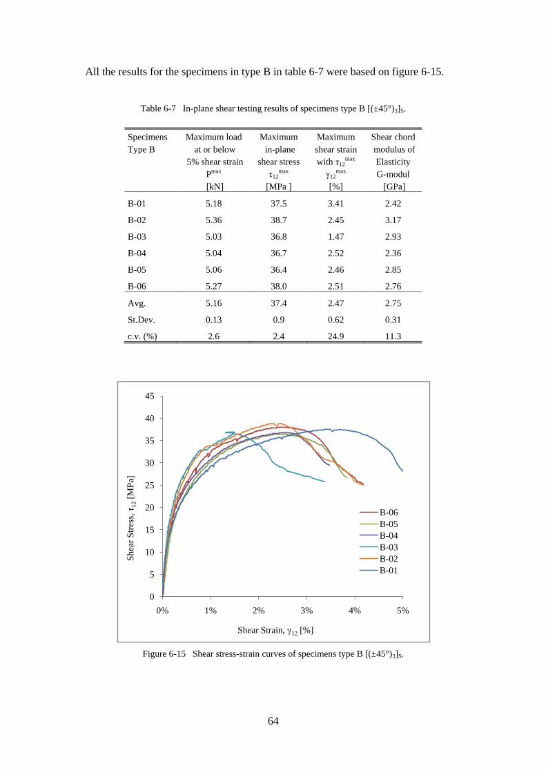
64
All the results for the specimens in type B in table 6-7 were based on figure 6-15.
Table 6-7 In-plane shear testing results of specimens type B [(±45°)3]S.
Specimens Maximum load Maximum Maximum Shear chord Type B at or below in-plane shear strain modulus of
5% shear strain shear stress with τ12
max Elasticity
Pmax τ12
max γ12max G-modul
[kN] [MPa ] [%] [GPa]
B-01 5.18 37.5 3.41 2.42
B-02 5.36 38.7 2.45 3.17
B-03 5.03 36.8 1.47 2.93
B-04 5.04 36.7 2.52 2.36
B-05 5.06 36.4 2.46 2.85
B-06 5.27 38.0 2.51 2.76
Avg. 5.16 37.4 2.47 2.75
St.Dev. 0.13 0.9 0.62 0.31
c.v. (%) 2.6 2.4 24.9 11.3
Figure 6-15 Shear stress-strain curves of specimens type B [(±45°)3]S.
0
5
10
15
20
25
30
35
40
45
0% 1% 2% 3% 4% 5%
Shea
r Stre
ss, τ
12[M
Pa]
Shear Strain, γ12 [%]
B-06B-05B-04B-03B-02B-01
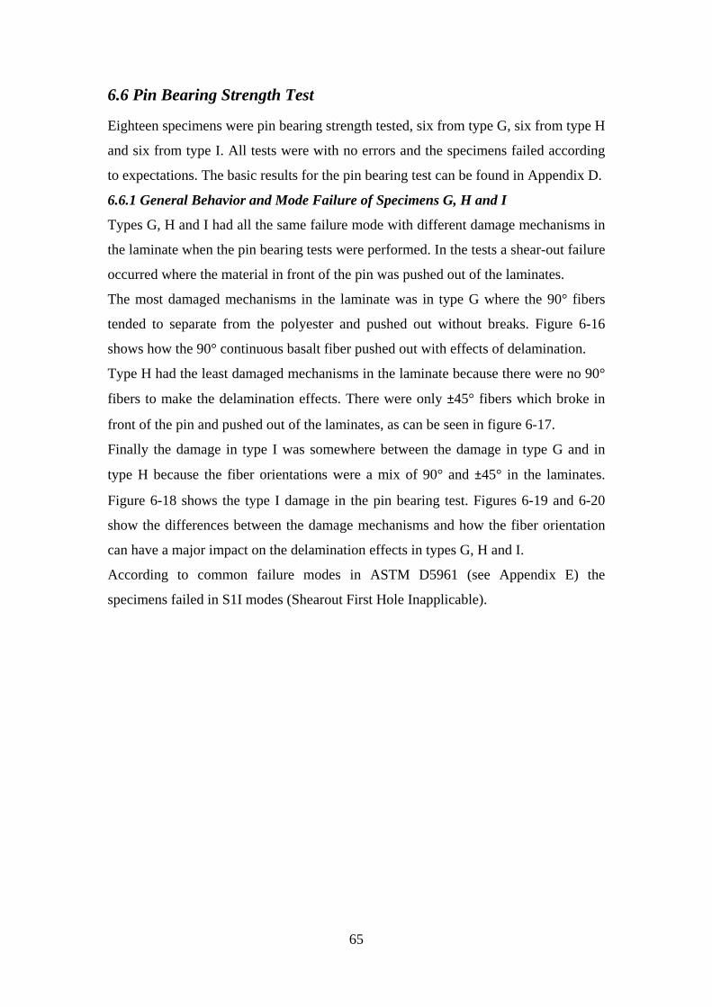
65
6.6 Pin Bearing Strength Test
Eighteen specimens were pin bearing strength tested, six from type G, six from type H
and six from type I. All tests were with no errors and the specimens failed according
to expectations. The basic results for the pin bearing test can be found in Appendix D.
6.6.1 General Behavior and Mode Failure of Specimens G, H and I
Types G, H and I had all the same failure mode with different damage mechanisms in
the laminate when the pin bearing tests were performed. In the tests a shear-out failure
occurred where the material in front of the pin was pushed out of the laminates.
The most damaged mechanisms in the laminate was in type G where the 90° fibers
tended to separate from the polyester and pushed out without breaks. Figure 6-16
shows how the 90° continuous basalt fiber pushed out with effects of delamination.
Type H had the least damaged mechanisms in the laminate because there were no 90°
fibers to make the delamination effects. There were only ±45° fibers which broke in
front of the pin and pushed out of the laminates, as can be seen in figure 6-17.
Finally the damage in type I was somewhere between the damage in type G and in
type H because the fiber orientations were a mix of 90° and ±45° in the laminates.
Figure 6-18 shows the type I damage in the pin bearing test. Figures 6-19 and 6-20
show the differences between the damage mechanisms and how the fiber orientation
can have a major impact on the delamination effects in types G, H and I.
According to common failure modes in ASTM D5961 (see Appendix E) the
specimens failed in S1I modes (Shearout First Hole Inapplicable).
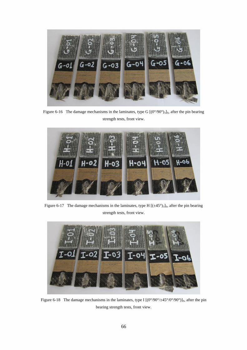
66
Figure 6-16 The damage mechanisms in the laminates, type G [(0°/90°)3]S, after the pin bearing
strength tests, front view.
Figure 6-17 The damage mechanisms in the laminates, type H [(±45°)3]S, after the pin bearing
strength tests, front view.
Figure 6-18 The damage mechanisms in the laminates, type I [(0°/90°/±45°/0°/90°)]S, after the pin
bearing strength tests, front view.
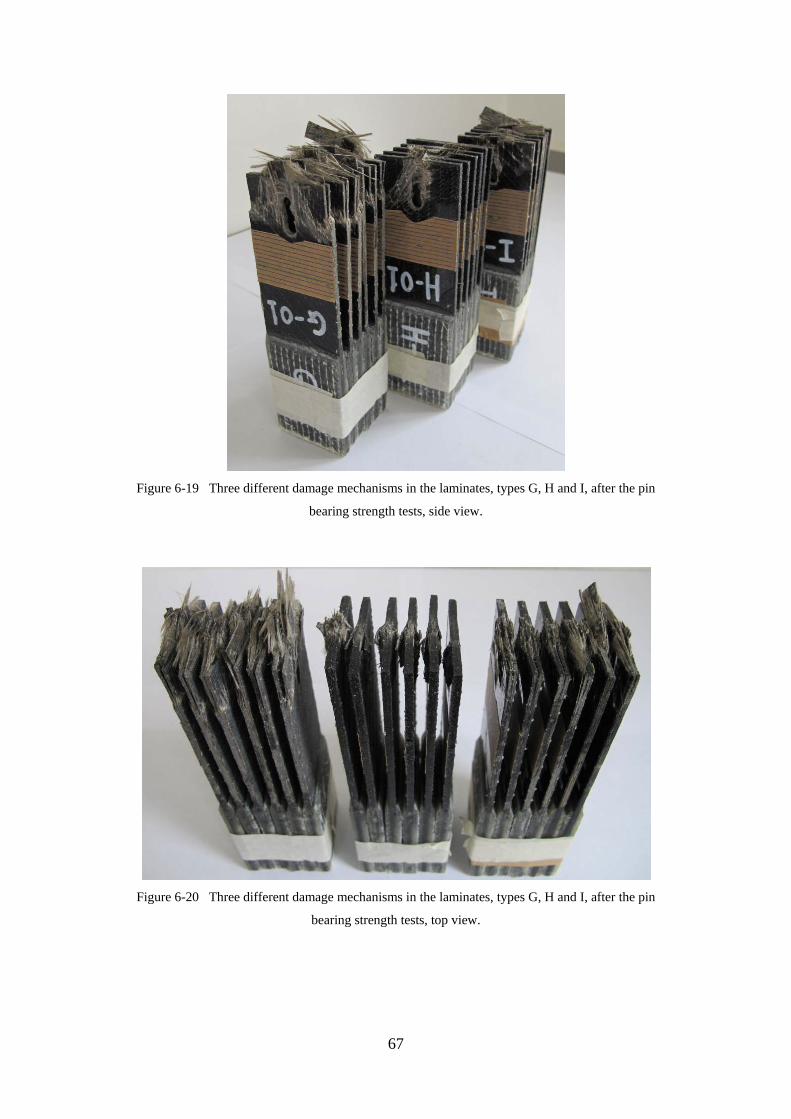
67
Figure 6-19 Three different damage mechanisms in the laminates, types G, H and I, after the pin
bearing strength tests, side view.
Figure 6-20 Three different damage mechanisms in the laminates, types G, H and I, after the pin
bearing strength tests, top view.
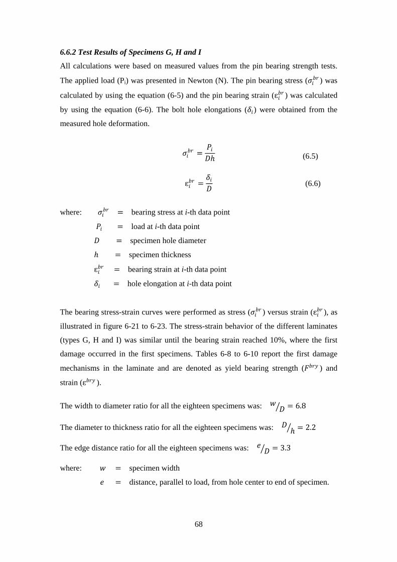
68
6.6.2 Test Results of Specimens G, H and I
All calculations were based on measured values from the pin bearing strength tests.
The applied load (Pi) was presented in Newton (N). The pin bearing stress (𝜎𝜎𝑖𝑖𝑏𝑏𝑏𝑏 ) was
calculated by using the equation (6-5) and the pin bearing strain (ɛ𝑖𝑖𝑏𝑏𝑏𝑏 ) was calculated
by using the equation (6-6). The bolt hole elongations (𝛿𝛿𝑖𝑖) were obtained from the
measured hole deformation.
𝜎𝜎𝑖𝑖𝑏𝑏𝑏𝑏 =𝑃𝑃𝑖𝑖𝐷𝐷ℎ
ɛ𝑖𝑖𝑏𝑏𝑏𝑏 =𝛿𝛿𝑖𝑖𝐷𝐷
where: 𝜎𝜎𝑖𝑖𝑏𝑏𝑏𝑏 = bearing stress at i-th data point
𝑃𝑃𝑖𝑖 = load at i-th data point
𝐷𝐷 = specimen hole diameter
ℎ = specimen thickness
ɛ𝑖𝑖𝑏𝑏𝑏𝑏 = bearing strain at i-th data point
𝛿𝛿𝑖𝑖 = hole elongation at i-th data point
The bearing stress-strain curves were performed as stress (𝜎𝜎𝑖𝑖𝑏𝑏𝑏𝑏 ) versus strain (ɛ𝑖𝑖𝑏𝑏𝑏𝑏 ), as
illustrated in figure 6-21 to 6-23. The stress-strain behavior of the different laminates
(types G, H and I) was similar until the bearing strain reached 10%, where the first
damage occurred in the first specimens. Tables 6-8 to 6-10 report the first damage
mechanisms in the laminate and are denoted as yield bearing strength (𝐹𝐹𝑏𝑏𝑏𝑏𝑦𝑦 ) and
strain (ɛ𝑏𝑏𝑏𝑏𝑦𝑦 ).
The width to diameter ratio for all the eighteen specimens was: 𝑤𝑤 𝐷𝐷� = 6.8 The diameter to thickness ratio for all the eighteen specimens was: 𝐷𝐷 ℎ� = 2.2 The edge distance ratio for all the eighteen specimens was: 𝑒𝑒 𝐷𝐷� = 3.3 where: 𝑤𝑤 = specimen width
𝑒𝑒 = distance, parallel to load, from hole center to end of specimen.
(6.5)
(6.6)
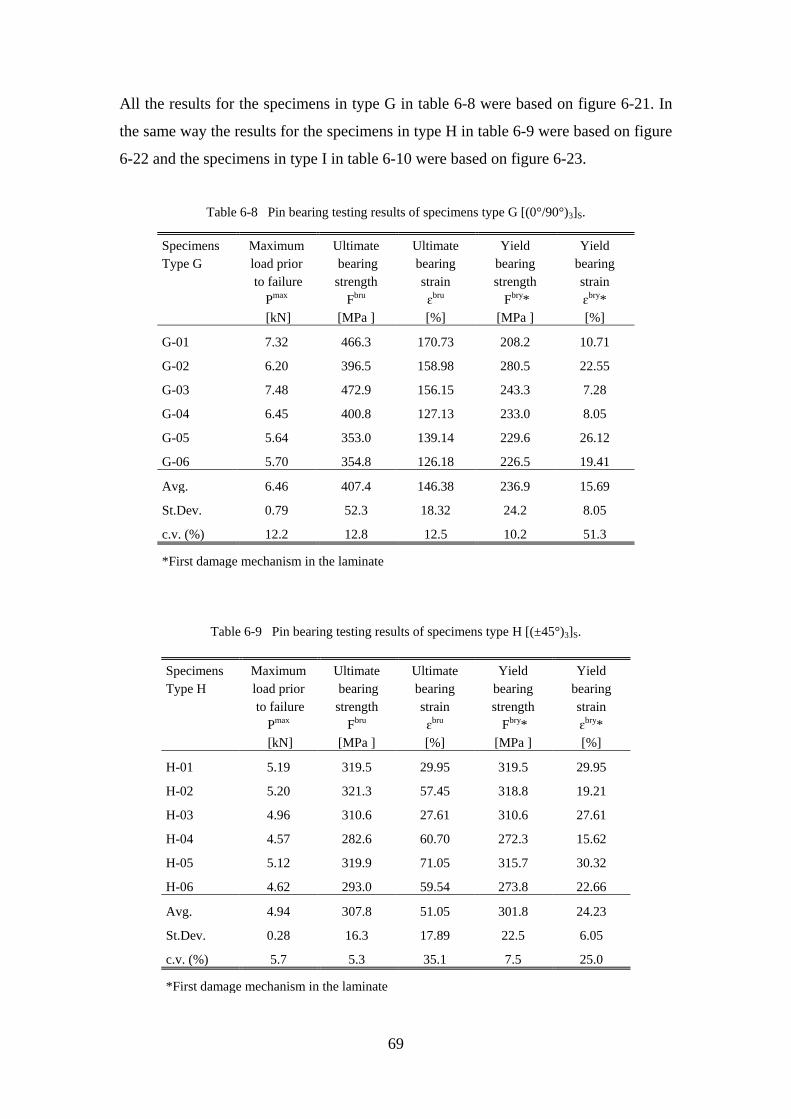
69
All the results for the specimens in type G in table 6-8 were based on figure 6-21. In
the same way the results for the specimens in type H in table 6-9 were based on figure
6-22 and the specimens in type I in table 6-10 were based on figure 6-23.
Table 6-8 Pin bearing testing results of specimens type G [(0°/90°)3]S.
Specimens Maximum Ultimate Ultimate Yield Yield Type G load prior bearing bearing bearing bearing
to failure strength strain strength strain
Pmax Fbru ɛbru Fbry* ɛbry*
[kN] [MPa ] [%] [MPa ] [%]
G-01 7.32 466.3 170.73 208.2 10.71
G-02 6.20 396.5 158.98 280.5 22.55
G-03 7.48 472.9 156.15 243.3 7.28
G-04 6.45 400.8 127.13 233.0 8.05
G-05 5.64 353.0 139.14 229.6 26.12
G-06 5.70 354.8 126.18 226.5 19.41
Avg. 6.46 407.4 146.38 236.9 15.69
St.Dev. 0.79 52.3 18.32 24.2 8.05
c.v. (%) 12.2 12.8 12.5 10.2 51.3
*First damage mechanism in the laminate
Table 6-9 Pin bearing testing results of specimens type H [(±45°)3]S.
Specimens Maximum Ultimate Ultimate Yield Yield Type H load prior bearing bearing bearing bearing
to failure strength strain strength strain
Pmax Fbru ɛbru Fbry* ɛbry*
[kN] [MPa ] [%] [MPa ] [%]
H-01 5.19 319.5 29.95 319.5 29.95
H-02 5.20 321.3 57.45 318.8 19.21
H-03 4.96 310.6 27.61 310.6 27.61
H-04 4.57 282.6 60.70 272.3 15.62
H-05 5.12 319.9 71.05 315.7 30.32
H-06 4.62 293.0 59.54 273.8 22.66
Avg. 4.94 307.8 51.05 301.8 24.23
St.Dev. 0.28 16.3 17.89 22.5 6.05
c.v. (%) 5.7 5.3 35.1 7.5 25.0
*First damage mechanism in the laminate
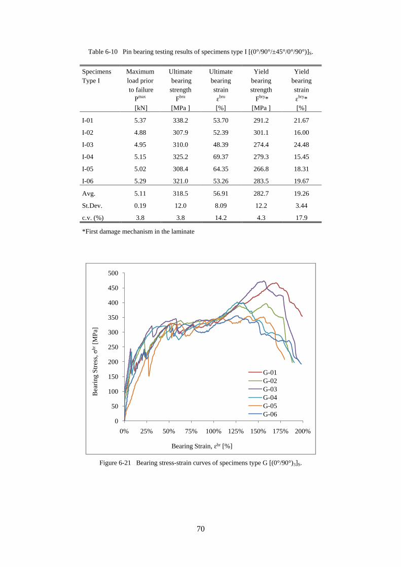
70
Table 6-10 Pin bearing testing results of specimens type I [(0°/90°/±45°/0°/90°)]S.
Specimens Maximum Ultimate Ultimate Yield Yield Type I load prior bearing bearing bearing bearing
to failure strength strain strength strain
Pmax Fbru ɛbru Fbry* ɛbry*
[kN] [MPa ] [%] [MPa ] [%]
I-01 5.37 338.2 53.70 291.2 21.67
I-02 4.88 307.9 52.39 301.1 16.00
I-03 4.95 310.0 48.39 274.4 24.48
I-04 5.15 325.2 69.37 279.3 15.45
I-05 5.02 308.4 64.35 266.8 18.31
I-06 5.29 321.0 53.26 283.5 19.67
Avg. 5.11 318.5 56.91 282.7 19.26
St.Dev. 0.19 12.0 8.09 12.2 3.44
c.v. (%) 3.8 3.8 14.2 4.3 17.9
*First damage mechanism in the laminate
Figure 6-21 Bearing stress-strain curves of specimens type G [(0°/90°)3]S.
0
50
100
150
200
250
300
350
400
450
500
0% 25% 50% 75% 100% 125% 150% 175% 200%
Bea
ring
Stre
ss, σ
br[M
Pa]
Bearing Strain, ɛbr [%]
G-01G-02G-03G-04G-05G-06
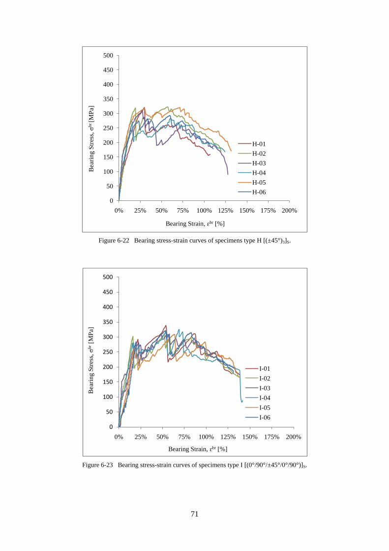
71
Figure 6-22 Bearing stress-strain curves of specimens type H [(±45°)3]S.
Figure 6-23 Bearing stress-strain curves of specimens type I [(0°/90°/±45°/0°/90°)]S.
0
50
100
150
200
250
300
350
400
450
500
0% 25% 50% 75% 100% 125% 150% 175% 200%
Bea
ring
Stre
ss, σ
br [M
Pa]
Bearing Strain, ɛbr [%]
H-01H-02H-03H-04H-05H-06
0
50
100
150
200
250
300
350
400
450
500
0% 25% 50% 75% 100% 125% 150% 175% 200%
Bea
ring
Stre
ss, σ
br[M
Pa]
Bearing Strain, ɛbr [%]
I-01I-02I-03I-04I-05I-06
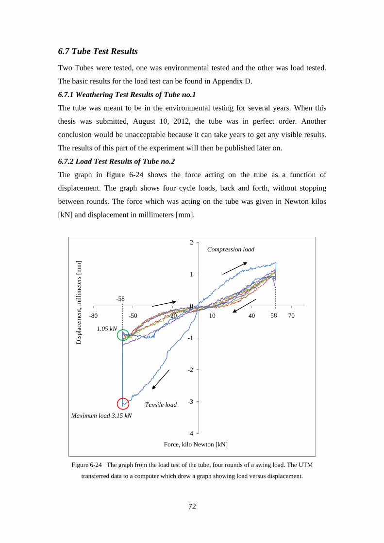
72
6.7 Tube Test Results
Two Tubes were tested, one was environmental tested and the other was load tested.
The basic results for the load test can be found in Appendix D.
6.7.1 Weathering Test Results of Tube no.1
The tube was meant to be in the environmental testing for several years. When this
thesis was submitted, August 10, 2012, the tube was in perfect order. Another
conclusion would be unacceptable because it can take years to get any visible results.
The results of this part of the experiment will then be published later on.
6.7.2 Load Test Results of Tube no.2
The graph in figure 6-24 shows the force acting on the tube as a function of
displacement. The graph shows four cycle loads, back and forth, without stopping
between rounds. The force which was acting on the tube was given in Newton kilos
[kN] and displacement in millimeters [mm].
Figure 6-24 The graph from the load test of the tube, four rounds of a swing load. The UTM
transferred data to a computer which drew a graph showing load versus displacement.
-4
-3
-2
-1
0
1
2
-80 -50 -20 10 40 70
Dis
plac
emen
t, m
illim
eter
s [m
m]
Force, kilo Newton [kN]
Compression load
Tensile load
Maximum load 3.15 kN
1.05 kN
-58
58
73
The graph in figure 6-24 shows that the greatest force acting on the tube was 3.15 kN
(shown in the red circle) when the tube moved about 58 mm at the top to the left in
the first cycle. Following this high force on the tube, the force fell down suddenly to
1.05 kN (shown in the green circle in figure 6-24). This force was the greatest force
which occurred in the load test. Closer inspection of the tube after the load test
showed that the glue in the iron pipe (fastener) between the tube and the UTM failed.
When the glue failed, the moment was reduced and the tube began to rotate slightly in
the fastener.
6.8 Summary
• The composite density, the weight and volume ratio for the basalt fiber and the
polyester resin were reported.
• The results of the tensile tests were reported (specimens types A and C).
• The results of the compression tests were reported (specimens types D and E).
• The results of the in-plane shear tests were reported (specimens type B).
• The results of the pin bearing tests were reported (specimens type G, H and I).
• The result of the tube in the load test was reported.
74
Discussion
7.1 General
This section presents a general discussion of the results and their interpretation.
7.2 Conclusion of Research
7.2.1 Constituent Content Determination Conclusion
The ratio between the fiber and resin has a major impact on strength and stiffness in a
composite material (Yuhazri, M. & Sihombing, H., n.d.). The most important factor in
the ratio between the fiber and resin is the volume fraction of reinforcing fibers. As
pointed out in section 2.3.1, the volume fraction of reinforcing fibers is used to
calculate the composite properties. Manufacturing processes such as Vacuum Infusion
generally give a higher volume fraction of reinforcing fibers than the Hand Lay-up
process using composite materials (Tsai, S.W., 1979, p. 251). The fiber volume
fraction for Vacuum Infusion is generally 50% or higher and for Hand Lay-up it is
normally less than 50%.
The forty-eight specimens, which were cut out of the two thin plates and made by the
Vacuum Infusion process, had 50.68 ± 0.45% a basalt fiber volume which is an
acceptable value. The tubes were made with the Hand Lay-up process and the basalt
fiber volume fraction was about 38%, which is also an acceptable value.
7.2.2 Tensile Test Conclusion of Specimens A and C
In the tensile test delamination occurred in all specimens where the basalt fibers
tended to separate from the polyester resin. Because of that, the adhesion between the
polyester resin and basalt fiber was the weakest factor in the composite material. A
resin with good adhesion with fiber can give more strength and stiffness in the
laminate; for example an epoxy resin gives better composite strength and stiffness
than a vinylester resin (Colombo et al., 2012). With this in mind, the resin can reduce
the strength and stiffness in a composite material.
The ultimate tensile strength for type A became 19.6% stronger than type C. The
tensile Young’s modulus became 25.8% higher in type A than in type C. This
conclusion should fit the theory (see section 2.3) because type A had more layers with
fiber orientation in a 0° direction. The ultimate tensile strain was around 2.8% for
both type A and type C. That is a little bit lower than ultimate tensile strain in dry
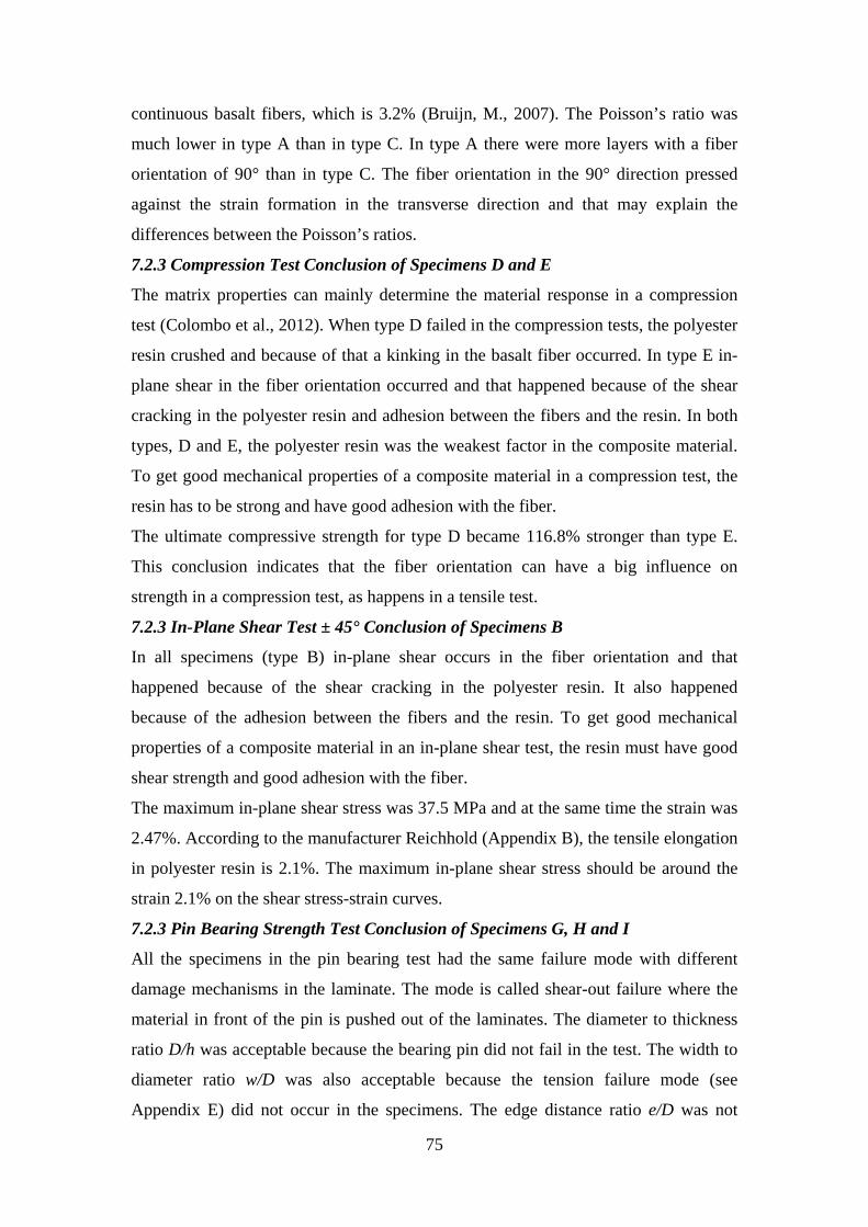
75
continuous basalt fibers, which is 3.2% (Bruijn, M., 2007). The Poisson’s ratio was
much lower in type A than in type C. In type A there were more layers with a fiber
orientation of 90° than in type C. The fiber orientation in the 90° direction pressed
against the strain formation in the transverse direction and that may explain the
differences between the Poisson’s ratios.
7.2.3 Compression Test Conclusion of Specimens D and E
The matrix properties can mainly determine the material response in a compression
test (Colombo et al., 2012). When type D failed in the compression tests, the polyester
resin crushed and because of that a kinking in the basalt fiber occurred. In type E in-
plane shear in the fiber orientation occurred and that happened because of the shear
cracking in the polyester resin and adhesion between the fibers and the resin. In both
types, D and E, the polyester resin was the weakest factor in the composite material.
To get good mechanical properties of a composite material in a compression test, the
resin has to be strong and have good adhesion with the fiber.
The ultimate compressive strength for type D became 116.8% stronger than type E.
This conclusion indicates that the fiber orientation can have a big influence on
strength in a compression test, as happens in a tensile test.
7.2.3 In-Plane Shear Test ± 45° Conclusion of Specimens B
In all specimens (type B) in-plane shear occurs in the fiber orientation and that
happened because of the shear cracking in the polyester resin. It also happened
because of the adhesion between the fibers and the resin. To get good mechanical
properties of a composite material in an in-plane shear test, the resin must have good
shear strength and good adhesion with the fiber.
The maximum in-plane shear stress was 37.5 MPa and at the same time the strain was
2.47%. According to the manufacturer Reichhold (Appendix B), the tensile elongation
in polyester resin is 2.1%. The maximum in-plane shear stress should be around the
strain 2.1% on the shear stress-strain curves.
7.2.3 Pin Bearing Strength Test Conclusion of Specimens G, H and I
All the specimens in the pin bearing test had the same failure mode with different
damage mechanisms in the laminate. The mode is called shear-out failure where the
material in front of the pin is pushed out of the laminates. The diameter to thickness
ratio D/h was acceptable because the bearing pin did not fail in the test. The width to
diameter ratio w/D was also acceptable because the tension failure mode (see
Appendix E) did not occur in the specimens. The edge distance ratio e/D was not
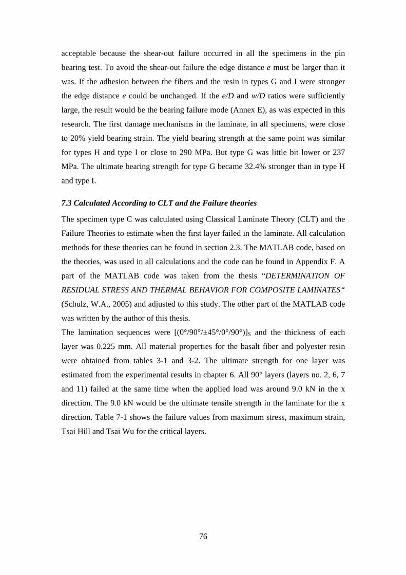
76
acceptable because the shear-out failure occurred in all the specimens in the pin
bearing test. To avoid the shear-out failure the edge distance e must be larger than it
was. If the adhesion between the fibers and the resin in types G and I were stronger
the edge distance e could be unchanged. If the e/D and w/D ratios were sufficiently
large, the result would be the bearing failure mode (Annex E), as was expected in this
research. The first damage mechanisms in the laminate, in all specimens, were close
to 20% yield bearing strain. The yield bearing strength at the same point was similar
for types H and type I or close to 290 MPa. But type G was little bit lower or 237
MPa. The ultimate bearing strength for type G became 32.4% stronger than in type H
and type I.
7.3 Calculated According to CLT and the Failure theories
The specimen type C was calculated using Classical Laminate Theory (CLT) and the
Failure Theories to estimate when the first layer failed in the laminate. All calculation
methods for these theories can be found in section 2.3. The MATLAB code, based on
the theories, was used in all calculations and the code can be found in Appendix F. A
part of the MATLAB code was taken from the thesis “DETERMINATION OF
RESIDUAL STRESS AND THERMAL BEHAVIOR FOR COMPOSITE LAMINATES“
(Schulz, W.A., 2005) and adjusted to this study. The other part of the MATLAB code
was written by the author of this thesis.
The lamination sequences were [(0°/90°/±45°/0°/90°)]S and the thickness of each
layer was 0.225 mm. All material properties for the basalt fiber and polyester resin
were obtained from tables 3-1 and 3-2. The ultimate strength for one layer was
estimated from the experimental results in chapter 6. All 90° layers (layers no. 2, 6, 7
and 11) failed at the same time when the applied load was around 9.0 kN in the x
direction. The 9.0 kN would be the ultimate tensile strength in the laminate for the x
direction. Table 7-1 shows the failure values from maximum stress, maximum strain,
Tsai Hill and Tsai Wu for the critical layers.
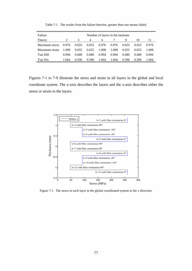
77
Table 7-1 The results from the failure theories, greater than one means failed.
Failure Number of layers in the laminate Theory 2 3 4 6 7 9 10 11 Maximum stress 0.976 0.655 0.655 0.976 0.976 0.655 0.655 0.976 Maximum strain 1.008 0.655 0.655 1.008 1.008 0.655 0.655 1.008 Tsai Hill 0.994 0.680 0.680 0.994 0.994 0.680 0.680 0.994 Tsai Wu 1.064 0.596 0.596 1.064 1.064 0.596 0.596 1.064
Figures 7-1 to 7-9 illustrate the stress and strain in all layers in the global and local
coordinate system. The y-axis describes the layers and the x-axis describes either the
stress or strain in the layers.
Figure 7-1 The stress in each layer in the global coordinated system in the x direction.
0 50 100 150 200 250 300-1.5
-1
-0.5
0
0.5
1
1.5
Stress (MPa)
Thic
knes
s (m
m)
Stress x
k=3 with fiber orientation +45°
k=6 with fiber orientation 90°
k=1 with fiber orientation 0°
k=9 with fiber orientation -45°
k=5 with fiber orientation 0°
k=2 with fiber orientation 90°
k=7 with fiber orientation 90°
k=8 with fiber orientation 0°
k=4 with fiber orientation -45°
k=10 with fiber orientation +45°
k=11 with fiber orientation 90°
k=12 with fiber orientation 0°
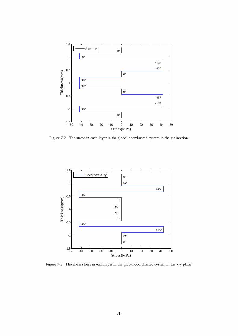
78
Figure 7-2 The stress in each layer in the global coordinated system in the y direction.
Figure 7-3 The shear stress in each layer in the global coordinated system in the x-y plane.
-50 -40 -30 -20 -10 0 10 20 30 40 50-1.5
-1
-0.5
0
0.5
1
1.5
Stress(MPa)
Thic
knes
s(m
m)
Stress y
-50 -40 -30 -20 -10 0 10 20 30 40 50-1.5
-1
-0.5
0
0.5
1
1.5
Stress(MPa)
Thic
knes
s(m
m)
Shear stress xy
0°
90°
+45°
-45°
0°
90°
90°
0°
-45°
+45°
90°
0°
0°
0°
+45°
-45°
90°
90°
90°
0°
-45°
+45°
90°
0°
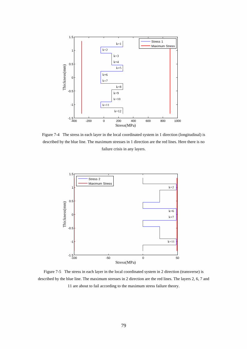
79
Figure 7-4 The stress in each layer in the local coordinated system in 1 direction (longitudinal) is
described by the blue line. The maximum stresses in 1 direction are the red lines. Here there is no
failure crisis in any layers.
Figure 7-5 The stress in each layer in the local coordinated system in 2 direction (transverse) is
described by the blue line. The maximum stresses in 2 direction are the red lines. The layers 2, 6, 7 and
11 are about to fail according to the maximum stress failure theory.
-400 -200 0 200 400 600 800 1000-1.5
-1
-0.5
0
0.5
1
1.5
Stress(MPa)
Thic
knes
s(m
m)
Stress 1Maximum Stress
-100 -50 0 50-1.5
-1
-0.5
0
0.5
1
1.5
Stress(MPa)
Thic
knes
s(m
m)
Stress 2Maximum Stress
k=1
k=2
k=3
k=4
k=5
k=6
k=7
k=8
k=9
k=10
k=11
k=12
k=2
k=6
k=7
k=11
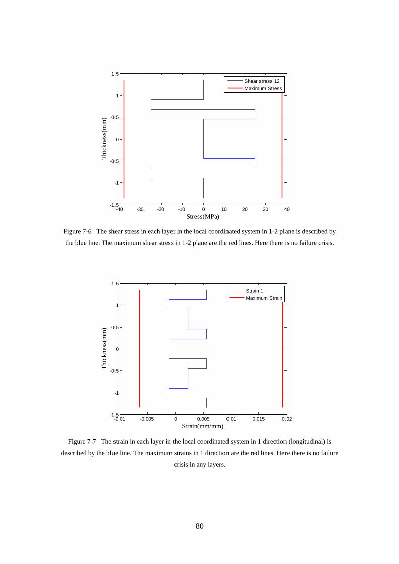
80
Figure 7-6 The shear stress in each layer in the local coordinated system in 1-2 plane is described by
the blue line. The maximum shear stress in 1-2 plane are the red lines. Here there is no failure crisis.
Figure 7-7 The strain in each layer in the local coordinated system in 1 direction (longitudinal) is
described by the blue line. The maximum strains in 1 direction are the red lines. Here there is no failure
crisis in any layers.
-40 -30 -20 -10 0 10 20 30 40-1.5
-1
-0.5
0
0.5
1
1.5
Stress(MPa)
Thic
knes
s(m
m)
Shear stress 12Maximum Stress
-0.01 -0.005 0 0.005 0.01 0.015 0.02-1.5
-1
-0.5
0
0.5
1
1.5
Strain(mm/mm)
Thic
knes
s(m
m)
Strain 1Maximum Strain
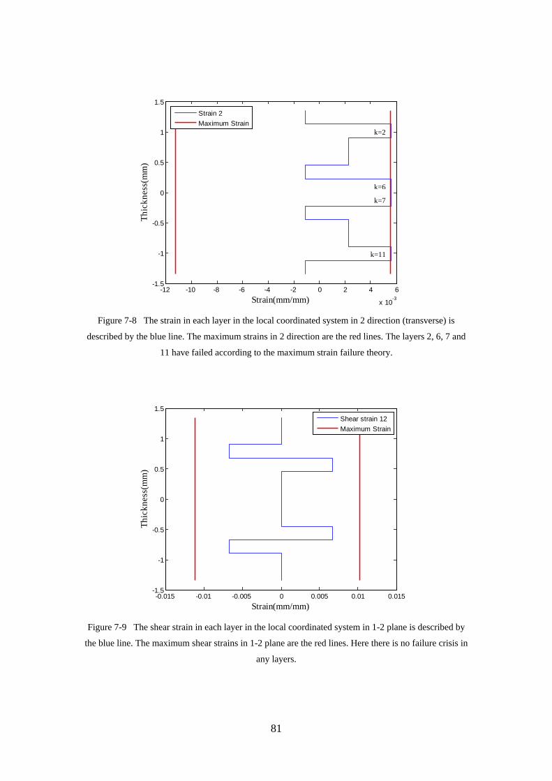
81
Figure 7-8 The strain in each layer in the local coordinated system in 2 direction (transverse) is
described by the blue line. The maximum strains in 2 direction are the red lines. The layers 2, 6, 7 and
11 have failed according to the maximum strain failure theory.
Figure 7-9 The shear strain in each layer in the local coordinated system in 1-2 plane is described by
the blue line. The maximum shear strains in 1-2 plane are the red lines. Here there is no failure crisis in
any layers.
-12 -10 -8 -6 -4 -2 0 2 4 6
x 10-3
-1.5
-1
-0.5
0
0.5
1
1.5
Strain(mm/mm)
Thic
knes
s(m
m)
Strain 2Maximum Strain
-0.015 -0.01 -0.005 0 0.005 0.01 0.015-1.5
-1
-0.5
0
0.5
1
1.5
Strain(mm/mm)
Thic
knes
s(m
m)
Shear strain 12Maximum Strain
k=2
k=6
k=7
k=11
82
7.4 Comparison with Other Composite materials
One way to estimate a quality of materials properties is to make comparisons with
other materials. The biaxial stitched basalt fabric BAS BI 600, in polyester resin, was
compared with other types of weave fabrics in epoxy resin. The composite properties
for the stitched basalt fabric were obtained from types A, D and B in the experiment
results.
The first two fabrics, which were compared to the stitched basalt fabric, were made of
continuous basalt fiber. The composite properties were obtained from a report from
Iran (Talebi Mazraehshahi & Zamani, 2010).The third fabric was made of continuous
E-glass fiber by Hexcel (ASTM International, 2002, pp. 428–437). The last fabric was
made of continuous carbon filaments made from PAM precursor (ASTM
International, 2002, pp. 276–285). The composite properties for the fabrics, E-glass
(E7781/EA9396) and carbon (T300 3k/EA9396), were obtained from The Composite
Materials Handbook-MIL17 (ASTM International, 2002).
The tensile test method ASTM D3039 and the in-plane shear test method ASTM
D3518 were used to find the composite properties in tensile and shear for all fabrics.
The compression tests methods ASTM D3410 and DIN EN 2850 were used to find
the composite properties in compression for all fabrics.
The comparison of composite properties of these different fabrics can be found in
table 7-2. The results in table 7-2 show that the composite density of basalt and E-
glass fabrics were similar, but 24.3% higher than the carbon fabric. The sum of
ultimate tensile strength of both directions (longitudinal and transverse direction) was
similar for all basalt fabrics. The stitched basalt fabric (which was examined in this
project) became 19.3% stronger than the E-glass fabric, but was 27.1% weaker than
carbon fabric. The ultimate tensile strain in the stitched basalt fabric became 25 to
160% higher than in the other fabrics. For that reason the tensile Young’s modulus of
elasticity was lowest in the stitched basalt fabric in comparison to the other fabrics.
The stitched basalt fabric was reinforced in polyester resin and the other fabrics were
reinforced in epoxy resin. The epoxy resin is generally stronger then polyester resin.
That can be the main reason for how low the ultimate compression strength and shear
Young’s modulus of elasticity was in the stitched basalt fabric.
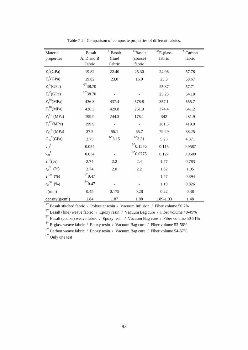
83
Table 7-2 Comparison of composite properties of different fabrics.
Material 1*Basalt 2*Basalt 3*Basalt 4*E-glass 5*Carbon properties A, D and B (fine) (coarse) fabric fabric Fabric Fabric fabric
E1t(GPa) 19.82 22.40 25.30 24.96 57.78
E2t(GPa) 19.82 23.0 16.0 25.3 58.67
E1c(GPa) 6*38.70 - - 25.37 57.71
E2c(GPa) 6*38.70 - - 25.23 54.19
F1tu(MPa) 436.3 437.4 578.8 357.1 555.7
F2tu(MPa) 436.3 429.8 251.9 374.4 641.2
F1cu (MPa) 199.9 244.3 175.1 342 481.9
F2cu(MPa) 199.9 - - 281.3 419.9
F12su(MPa) 37.5 55.1 65.7 79.29 88.25
G12s(GPa) 2.75 6*3.15 6*3.31 5.23 4.371
ν12t 0.054 - 6*0.1576 0.115 0.0587
ν21t 0.054 - 6*0.0775 0.127 0.0509
ɛ1tu(%) 2.74 2.2 2.4 1.77 0.783
ɛ2tu (%) 2.74 2.0 2.2 1.82 1.05
ɛ1cu (%) 6*0.47 - - 1.47 0.894
ɛ2cu (%) 6*0.47 - - 1.19 0.826
t (mm) 0.45 0.175 0.28 0.22 0.38
density(g/cm3) 1.84 1.87 1.88 1.89-1.93 1.48 1* Basalt stitched fabric / Polyester resin / Vacuum Infusion / Fiber volume 50.7% 2* Basalt (fine) weave fabric / Epoxy resin / Vacuum Bag cure / Fiber volume 48-49% 3* Basalt (coarse) weave fabric / Epoxy resin / Vacuum Bag cure / Fiber volume 50-51% 4* E-glass weave fabric / Epoxy resin / Vacuum Bag cure / Fiber volume 52-56% 5* Carbon weave fabric / Epoxy resin / Vacuum Bag cure / Fiber volume 54-57% 6* Only one test
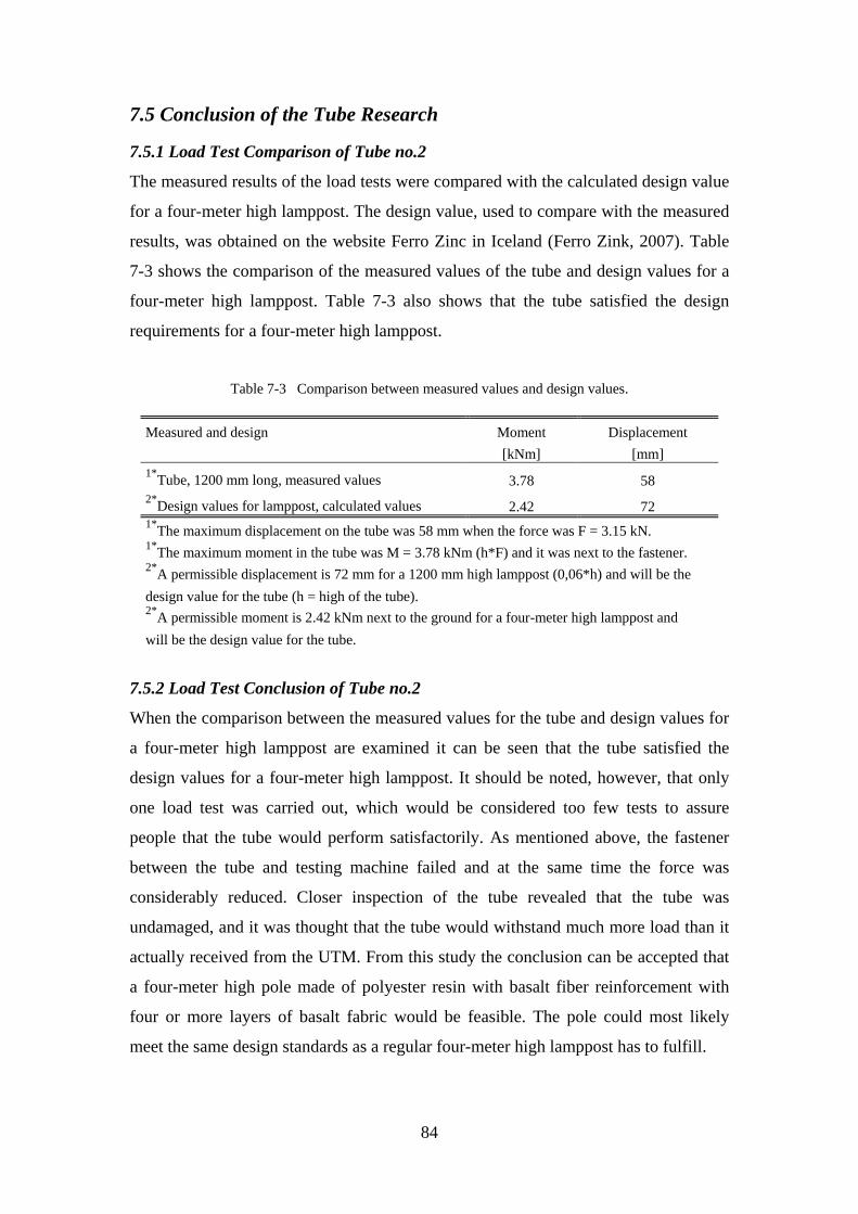
84
7.5 Conclusion of the Tube Research
7.5.1 Load Test Comparison of Tube no.2
The measured results of the load tests were compared with the calculated design value
for a four-meter high lamppost. The design value, used to compare with the measured
results, was obtained on the website Ferro Zinc in Iceland (Ferro Zink, 2007). Table
7-3 shows the comparison of the measured values of the tube and design values for a
four-meter high lamppost. Table 7-3 also shows that the tube satisfied the design
requirements for a four-meter high lamppost.
Table 7-3 Comparison between measured values and design values.
Measured and design Moment Displacement [kNm] [mm] 1*Tube, 1200 mm long, measured values 3.78 58 2*Design values for lamppost, calculated values 2.42 72 1*The maximum displacement on the tube was 58 mm when the force was F = 3.15 kN. 1*The maximum moment in the tube was M = 3.78 kNm (h*F) and it was next to the fastener. 2*A permissible displacement is 72 mm for a 1200 mm high lamppost (0,06*h) and will be the design value for the tube (h = high of the tube). 2*A permissible moment is 2.42 kNm next to the ground for a four-meter high lamppost and will be the design value for the tube.
7.5.2 Load Test Conclusion of Tube no.2
When the comparison between the measured values for the tube and design values for
a four-meter high lamppost are examined it can be seen that the tube satisfied the
design values for a four-meter high lamppost. It should be noted, however, that only
one load test was carried out, which would be considered too few tests to assure
people that the tube would perform satisfactorily. As mentioned above, the fastener
between the tube and testing machine failed and at the same time the force was
considerably reduced. Closer inspection of the tube revealed that the tube was
undamaged, and it was thought that the tube would withstand much more load than it
actually received from the UTM. From this study the conclusion can be accepted that
a four-meter high pole made of polyester resin with basalt fiber reinforcement with
four or more layers of basalt fabric would be feasible. The pole could most likely
meet the same design standards as a regular four-meter high lamppost has to fulfill.
85
7.6 Summary
• Vacuum Infusion processes gave a 50.68 ±0.45 % basalt fiber volume and
Hand Lay-up processes gave a 38% basalt fiber volume.
• In the tensile test specimens A became 19.6% stronger than specimens C.
• In the compression test specimens D became 116.8% stronger than specimens
E.
• In the in-plane shear test the shear strength was low because of the polyester
resin and adhesion between the fibers and the resin.
• In the pin bearing test the first damage mechanisms in the laminate were close
to 20% bearing strain.
• In calculations according to Classical Laminate Theory the first layers failed at
9.0 kN in specimens C.
• In the comparison, the stitched basalt fabric (which was examined in this
project) became 19.3% stronger than the E-glass fabric.
• The basalt tube could most likely satisfy the design values for a four-meter
high lamppost.
86
Summary
8.1 General
The results of the experiments in this thesis indicate that continuous basalt fibers, as
reinforcement material in polymer matrix, can be used as a composite material for
structural design. The static uniaxial test showed that basalt fiber was stronger than E-
glass fiber. As pointed out in chapter 2, glass fibers are the most used fiber in the
world in all kinds of structures and basalt fiber could possibly be used instead of these
types of fibers. In addition, the basalt tube was strong enough to be used as a regular
four-meter high lamppost. To ensure that basalt fiber could be used as a feasible
composite and reinforcement material in a matrix more and different types of testing
are required. But this study has shown that this composite material could be usable in
structures design and that further testing is justified.
8.2 Further Research
This study was concentrated on static testing to get basic results for the feasibility of
using continuous basalt fibers in polyester resin. To get more information about the
material properties for basalt fiber as a reinforcement material in matrix various other
tests could be performed. Here are a few of the experimental studies that could be
carried out:
• Carry out a dynamic load test. Because in reality the applied loads are usually
dynamical, for example because of wind load and earthquake load.
• Carry out a more static load test, for example a flexural test and a delamination
test. It is very important to investigate delamination in the material because it
continued to in the present experiment.
• Investigate the adhesion between the basalt fiber and other resin. The adhesion
between the basalt fiber and polyester resin was one of the weakest factors in
the experiment.
• Carry out a fatigue test. This is very important for structures that are under
variable continuous loads.
87
References ASTM D3039 / D3039M - 00 : Standard test method for tensile properties of polymer
matrix composite materials. (2000). West Conshohocken, PA: ASTM
International.
ASTM D3171 - 99 : Standard test method for constituent of composite materials.
(2000). West Conshohocken, PA: ASTM International.
ASTM D3410 / D3410M - 03 : Standard test method for compressive properties of
polymer matrix composite materials with unsupported gage section by shear
loading. (2003). West Conshohocken, PA: ASTM International.
ASTM D3518 / D3518M - 94 : Standard test method for in plane shear response of
polymer matrix composite materials by tensile test of a ±45° laminate. (1994).
West Conshohocken, PA: ASTM International.
ASTM D5961 / D5961M - 01 : Standard test method for bearing response of polymer
matrix composite laminates. (2001). West Conshohocken, PA: ASTM
International.
ASTM D695 - 02 : Standard test method for compressive properties of rigid plastics.
(2002). West Conshohocken, PA: ASTM International.
ASTM E111 - 97 : Standard test method for young’s modulus, tangent modulus, and
chord modulus. (1997). West Conshohocken, PA: ASTM International.
ASTM E132 - 04 : Standard test method for Poisson’s ratio at room temperature.
(2004). West Conshohocken, PA: ASTM International.
ASTM International. (2002). The composite materials handbook-MIL 17: Polymer
matrix composites: materials properties. West Conshohocken, PA: ASTM
International.
ASTM International. (2012). About ASTM International - ASTM overview.
Retrieved May 8, 2012, from http://www.astm.org/ABOUT/overview.html
88
Árnason, P. (2007). Plast 3. Reykjavík: Nýsköpunarmiðstöð Íslands.
Boeing. (n.d.). Commercial airplanes - 787 Dreamliner. Boeing 787. Retrieved May
31, 2012, from
http://www.boeing.com/commercial/787family/background.html
Bruijn, M. (2007). Evaluation of basalt continuous filament fibres in composite
material. Belgium: Universiteit Leuven. Retrieved from
http://www.basaltex.com/files/cms1/Report-Evaluation-of-Basalt-Continuous-
Filament-Fibres-in-composite-material_June%202007.pdf
Chang, Z. L., Zou, G. P., Chen, S., & Chen, L. (2011). The study of AE and ESSPI
technique on the CBF composite. Key Engineering Materials, 488-489, 436–
439. doi:10.4028/www.scientific.net/KEM.488-489.436
Chapter 4 failure theories. (n.d.). Retrieved May 4, 2012, from
http://www.docstoc.com/docs/101939810/Chapter-4-Failure-Theories
Colombo, C., Vergani, L., & Burman, M. (2012). Static and fatigue characterisation
of new basalt fibre reinforced composites. Composite Structures, 94(3), 1165–
1174. doi:10.1016/j.compstruct.2011.10.007
Europe’s first plastic bridge is open. (2010). Retrieved May 31, 2012, from
http://www.plasticseurope.co.uk/information-centre-
8484/news/archives/europes-first-plastic-bridge-is-open.aspx
Ferro Zink. (2007). Ljósastaur 4x60. Retrieved June 8, 2012, from
http://www.ferro.is/ferrozink/upload/files/acrobat/framleidsluvorur/102-
staur_4x60_ch.pdf
Greene, E. (n.d.). Marine composites. Retrieved May 1, 2012, from
http://www.marinecomposites.com/PDF_Files/H_Micromechanics.pdf
Hyer, M. (2008). Stress analysis of fiber-reinforced composite materials (Updated.).
Lancaster, PA: Destech Pubns Inc.
89
Jones, R. M. (1998). Mechanics of composite materials (2 Sub.). Blacksburg, VA:
CRC Press.
Kamenny Vek. (2009). Advanced basalt fiber. Basfiber. Retrieved May 9, 2012, from
http://www.basfiber.com/
Kant, T. (2010). Composite mechanics in the last 50 years. Retrieved May 6, 2012,
from http://www.ircc.iitb.ac.in/IRCC-Webpage/PDF/TarunKant2010.pdf
Manjunatha, B. S., & Kant, T. (1992). A comparison of 9 and 16 node quadrilateral
elements based on higher-order laminate theories for estimation of transverse
stresses. Journal of Reinforced Plastics and Composites, 11(9), 968–1002.
doi:10.1177/073168449201100902
McGeorge, D., & Höyning, B. (n.d.). NATO-RTO. Retrieved May 31, 2012, from
http://research.dnv.com/euclid_rtp3.21/PW_Tools/PWE/Input/NATO-RTO-
DagMcGeorgeBjornHoyning.pdf
Meunier, M., & Knibbs, S. (2007). Design tools for fibre reinforced polymer
structures. National Composites Network.
Parnas, R., & Shaw, M. (2007). Basalt fiber reinforced polymer composites ( No. 03-
7). New England, MA: Transportation Consortium.
Reissner, E., & Stavsky, Y. (1961). Bending and stretching of certain types of
heterogeneous aeolotropic elastic plates. Journal of Applied Mechanics, 28(3),
402. doi:10.1115/1.3641719
Ross, A. (2006). Basalt fibers: Alternative to glass? Composites World. Retrieved
May 9, 2012, from http://www.compositesworld.com/articles/basalt-fibers-
alternative-to-glass
Schulz, W.A. (2005). Determination of residual stress and thermal behavior for
composite laminates (Master thesis). University of Florida, Florida. Retrieved
from http://ufdcimages.uflib.ufl.edu/UF/E0/01/04/06/00001/schulz_w.pdf
90
Shakespeare composite structures. (n.d.). Retrieved May 31, 2012, from
http://www.skp-cs.com/default.asp
SP Systems. (n.d.). Guide to composites. Retrieved from
http://www.bolton.ac.uk/codate/spguidetocomposites.pdf
Staab, G. H. (1999). Laminar composites. Woburn, MA: Butterworth-Heinemann.
Talebi Mazraehshahi, H., & Zamani, H. (2010). Investigation on mechanical
properties of basalt composite fabrics (experiment study). EPJ Web of
Conferences, 6, 20008. doi:10.1051/epjconf/20100620008
Tsai, S.W. (Ed.). (1979). Composite materials: Testing and design (fifth conference):
Stp 674. ASTM International.
Van de Velde, K., Kiekens, P., & Van Langenhove, L. (n.d.). Basalt fibres as
reinforcement-for composites. Belgium: Ghent University.
Yuhazri, M., & Sihombing, H. (n.d.). A comparison process between vacuum infusion
and hand lay-up method toward kenaf/polyester composites. International
Journal of Basic & Applied Sciences, 10(3), 63–66.
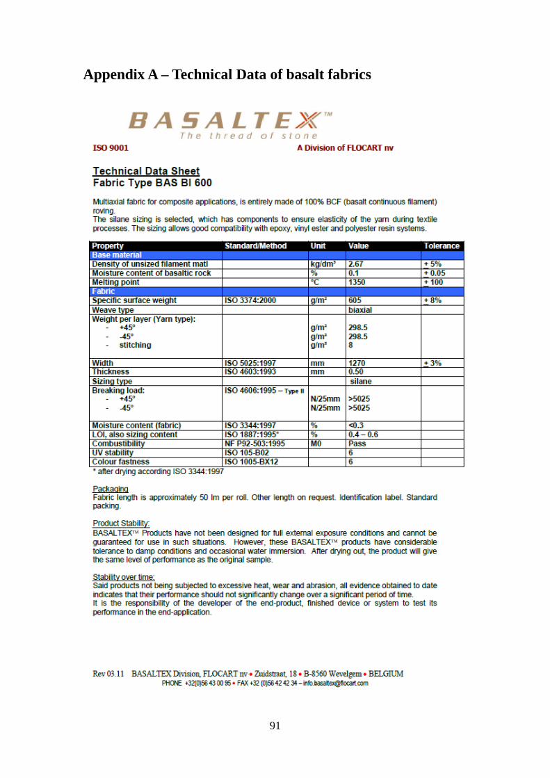
91
Appendix A – Technical Data of basalt fabrics
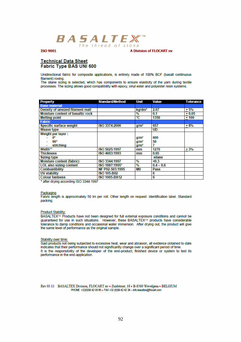
92
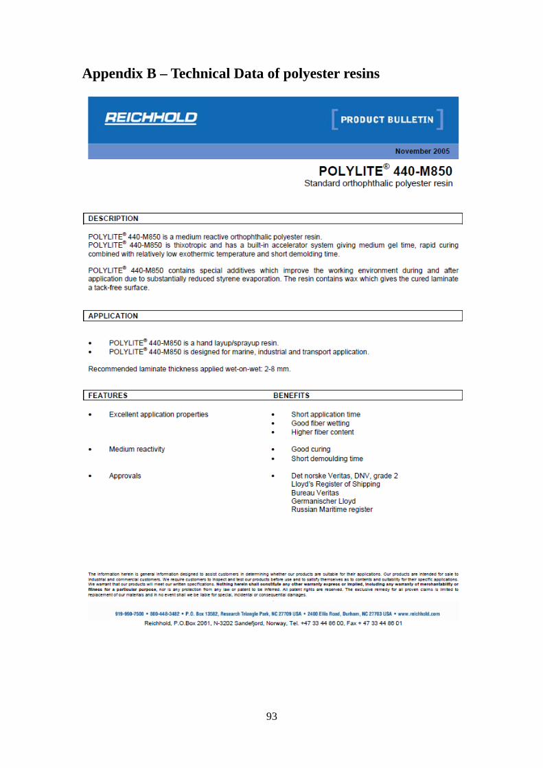
93
Appendix B – Technical Data of polyester resins

94
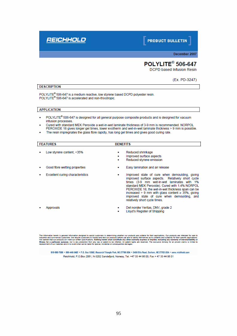
95
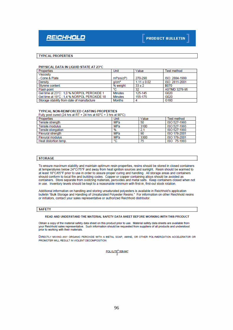
96
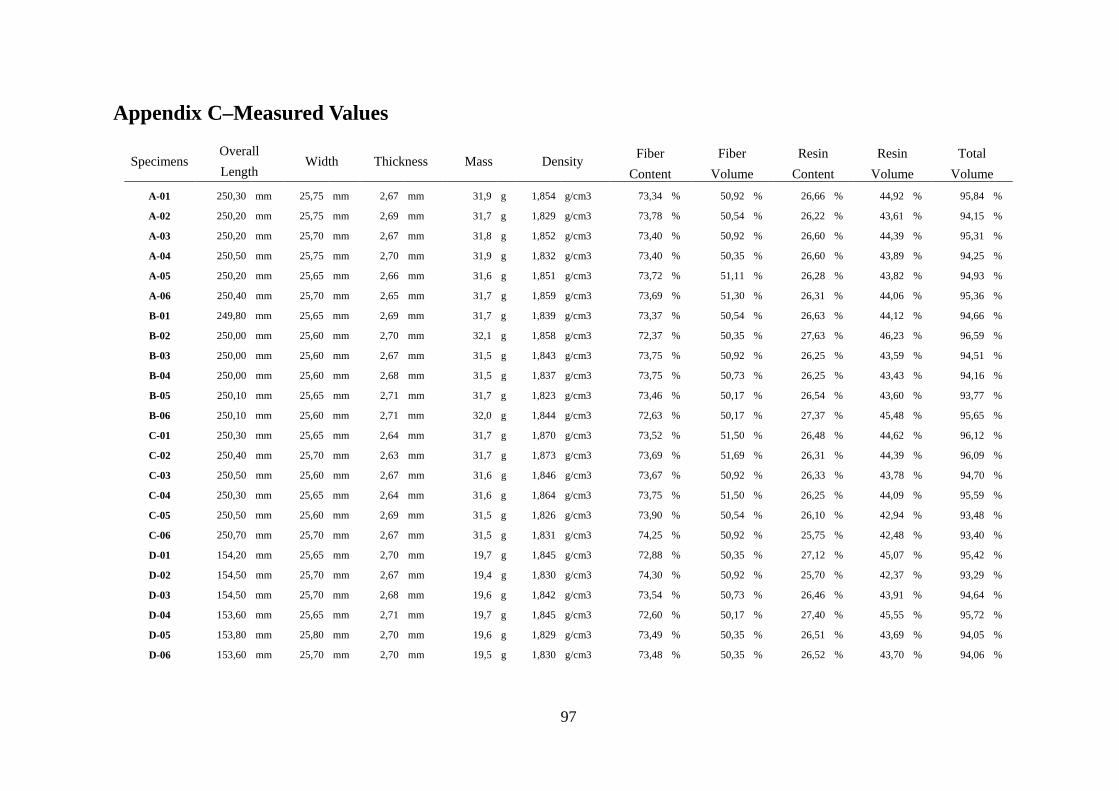
97
Appendix C–Measured Values
Specimens Overall
Width Thickness Mass Density Fiber Fiber Resin Resin Total Length Content Volume Content Volume Volume
A-01 250,30 mm 25,75 mm 2,67 mm 31,9 g 1,854 g/cm3 73,34 % 50,92 % 26,66 % 44,92 % 95,84 %
A-02 250,20 mm 25,75 mm 2,69 mm 31,7 g 1,829 g/cm3 73,78 % 50,54 % 26,22 % 43,61 % 94,15 %
A-03 250,20 mm 25,70 mm 2,67 mm 31,8 g 1,852 g/cm3 73,40 % 50,92 % 26,60 % 44,39 % 95,31 %
A-04 250,50 mm 25,75 mm 2,70 mm 31,9 g 1,832 g/cm3 73,40 % 50,35 % 26,60 % 43,89 % 94,25 %
A-05 250,20 mm 25,65 mm 2,66 mm 31,6 g 1,851 g/cm3 73,72 % 51,11 % 26,28 % 43,82 % 94,93 %
A-06 250,40 mm 25,70 mm 2,65 mm 31,7 g 1,859 g/cm3 73,69 % 51,30 % 26,31 % 44,06 % 95,36 %
B-01 249,80 mm 25,65 mm 2,69 mm 31,7 g 1,839 g/cm3 73,37 % 50,54 % 26,63 % 44,12 % 94,66 %
B-02 250,00 mm 25,60 mm 2,70 mm 32,1 g 1,858 g/cm3 72,37 % 50,35 % 27,63 % 46,23 % 96,59 %
B-03 250,00 mm 25,60 mm 2,67 mm 31,5 g 1,843 g/cm3 73,75 % 50,92 % 26,25 % 43,59 % 94,51 %
B-04 250,00 mm 25,60 mm 2,68 mm 31,5 g 1,837 g/cm3 73,75 % 50,73 % 26,25 % 43,43 % 94,16 %
B-05 250,10 mm 25,65 mm 2,71 mm 31,7 g 1,823 g/cm3 73,46 % 50,17 % 26,54 % 43,60 % 93,77 %
B-06 250,10 mm 25,60 mm 2,71 mm 32,0 g 1,844 g/cm3 72,63 % 50,17 % 27,37 % 45,48 % 95,65 %
C-01 250,30 mm 25,65 mm 2,64 mm 31,7 g 1,870 g/cm3 73,52 % 51,50 % 26,48 % 44,62 % 96,12 %
C-02 250,40 mm 25,70 mm 2,63 mm 31,7 g 1,873 g/cm3 73,69 % 51,69 % 26,31 % 44,39 % 96,09 %
C-03 250,50 mm 25,60 mm 2,67 mm 31,6 g 1,846 g/cm3 73,67 % 50,92 % 26,33 % 43,78 % 94,70 %
C-04 250,30 mm 25,65 mm 2,64 mm 31,6 g 1,864 g/cm3 73,75 % 51,50 % 26,25 % 44,09 % 95,59 %
C-05 250,50 mm 25,60 mm 2,69 mm 31,5 g 1,826 g/cm3 73,90 % 50,54 % 26,10 % 42,94 % 93,48 %
C-06 250,70 mm 25,70 mm 2,67 mm 31,5 g 1,831 g/cm3 74,25 % 50,92 % 25,75 % 42,48 % 93,40 %
D-01 154,20 mm 25,65 mm 2,70 mm 19,7 g 1,845 g/cm3 72,88 % 50,35 % 27,12 % 45,07 % 95,42 %
D-02 154,50 mm 25,70 mm 2,67 mm 19,4 g 1,830 g/cm3 74,30 % 50,92 % 25,70 % 42,37 % 93,29 %
D-03 154,50 mm 25,70 mm 2,68 mm 19,6 g 1,842 g/cm3 73,54 % 50,73 % 26,46 % 43,91 % 94,64 %
D-04 153,60 mm 25,65 mm 2,71 mm 19,7 g 1,845 g/cm3 72,60 % 50,17 % 27,40 % 45,55 % 95,72 %
D-05 153,80 mm 25,80 mm 2,70 mm 19,6 g 1,829 g/cm3 73,49 % 50,35 % 26,51 % 43,69 % 94,05 %
D-06 153,60 mm 25,70 mm 2,70 mm 19,5 g 1,830 g/cm3 73,48 % 50,35 % 26,52 % 43,70 % 94,06 %
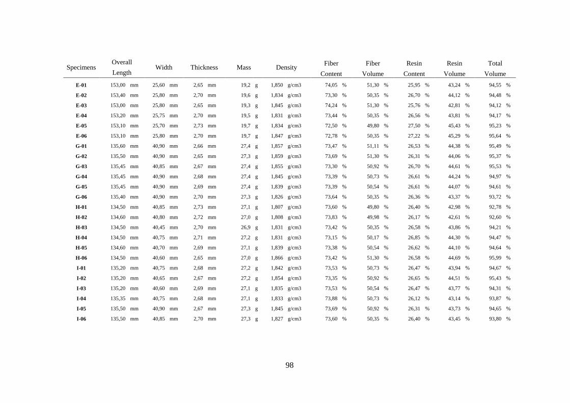
98
Specimens Overall
Width Thickness Mass Density Fiber Fiber Resin Resin Total Length Content Volume Content Volume Volume
E-01 153,00 mm 25,60 mm 2,65 mm 19,2 g 1,850 g/cm3 74,05 % 51,30 % 25,95 % 43,24 % 94,55 %
E-02 153,40 mm 25,80 mm 2,70 mm 19,6 g 1,834 g/cm3 73,30 % 50,35 % 26,70 % 44,12 % 94,48 %
E-03 153,00 mm 25,80 mm 2,65 mm 19,3 g 1,845 g/cm3 74,24 % 51,30 % 25,76 % 42,81 % 94,12 %
E-04 153,20 mm 25,75 mm 2,70 mm 19,5 g 1,831 g/cm3 73,44 % 50,35 % 26,56 % 43,81 % 94,17 %
E-05 153,10 mm 25,70 mm 2,73 mm 19,7 g 1,834 g/cm3 72,50 % 49,80 % 27,50 % 45,43 % 95,23 %
E-06 153,10 mm 25,80 mm 2,70 mm 19,7 g 1,847 g/cm3 72,78 % 50,35 % 27,22 % 45,29 % 95,64 %
G-01 135,60 mm 40,90 mm 2,66 mm 27,4 g 1,857 g/cm3 73,47 % 51,11 % 26,53 % 44,38 % 95,49 %
G-02 135,50 mm 40,90 mm 2,65 mm 27,3 g 1,859 g/cm3 73,69 % 51,30 % 26,31 % 44,06 % 95,37 %
G-03 135,45 mm 40,85 mm 2,67 mm 27,4 g 1,855 g/cm3 73,30 % 50,92 % 26,70 % 44,61 % 95,53 %
G-04 135,45 mm 40,90 mm 2,68 mm 27,4 g 1,845 g/cm3 73,39 % 50,73 % 26,61 % 44,24 % 94,97 %
G-05 135,45 mm 40,90 mm 2,69 mm 27,4 g 1,839 g/cm3 73,39 % 50,54 % 26,61 % 44,07 % 94,61 %
G-06 135,40 mm 40,90 mm 2,70 mm 27,3 g 1,826 g/cm3 73,64 % 50,35 % 26,36 % 43,37 % 93,72 %
H-01 134,50 mm 40,85 mm 2,73 mm 27,1 g 1,807 g/cm3 73,60 % 49,80 % 26,40 % 42,98 % 92,78 %
H-02 134,60 mm 40,80 mm 2,72 mm 27,0 g 1,808 g/cm3 73,83 % 49,98 % 26,17 % 42,61 % 92,60 %
H-03 134,50 mm 40,45 mm 2,70 mm 26,9 g 1,831 g/cm3 73,42 % 50,35 % 26,58 % 43,86 % 94,21 %
H-04 134,50 mm 40,75 mm 2,71 mm 27,2 g 1,831 g/cm3 73,15 % 50,17 % 26,85 % 44,30 % 94,47 %
H-05 134,60 mm 40,70 mm 2,69 mm 27,1 g 1,839 g/cm3 73,38 % 50,54 % 26,62 % 44,10 % 94,64 %
H-06 134,50 mm 40,60 mm 2,65 mm 27,0 g 1,866 g/cm3 73,42 % 51,30 % 26,58 % 44,69 % 95,99 %
I-01 135,20 mm 40,75 mm 2,68 mm 27,2 g 1,842 g/cm3 73,53 % 50,73 % 26,47 % 43,94 % 94,67 %
I-02 135,20 mm 40,65 mm 2,67 mm 27,2 g 1,854 g/cm3 73,35 % 50,92 % 26,65 % 44,51 % 95,43 %
I-03 135,20 mm 40,60 mm 2,69 mm 27,1 g 1,835 g/cm3 73,53 % 50,54 % 26,47 % 43,77 % 94,31 %
I-04 135,35 mm 40,75 mm 2,68 mm 27,1 g 1,833 g/cm3 73,88 % 50,73 % 26,12 % 43,14 % 93,87 %
I-05 135,50 mm 40,90 mm 2,67 mm 27,3 g 1,845 g/cm3 73,69 % 50,92 % 26,31 % 43,73 % 94,65 %
I-06 135,50 mm 40,85 mm 2,70 mm 27,3 g 1,827 g/cm3 73,60 % 50,35 % 26,40 % 43,45 % 93,80 %
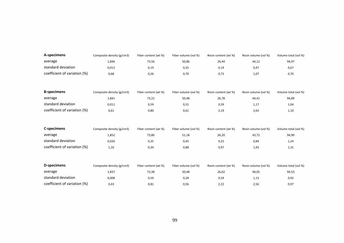
99
A-specimens Composite density (g/cm3)
Fiber content (wt %)
Fiber volume (vol %)
Resin content (wt %)
Resin volume (vol %)
Volume total (vol %)
average 1,846
73,56
50,86
26,44
44,12
94,97
standard deviation 0,012
0,19
0,35
0,19
0,47
0,67
coefficient of variation (%) 0,68
0,26
0,70
0,73
1,07
0,70
B-specimens Composite density (g/cm3)
Fiber content (wt %)
Fiber volume (vol %)
Resin content (wt %)
Resin volume (vol %)
Volume total (vol %)
average 1,841
73,22
50,48
26,78
44,41
94,89
standard deviation 0,011
0,59
0,31
0,59
1,17
1,04
coefficient of variation (%) 0,61
0,80
0,61
2,19
2,63
1,10
C-specimens Composite density (g/cm3)
Fiber content (wt %)
Fiber volume (vol %)
Resin content (wt %)
Resin volume (vol %)
Volume total (vol %)
average 1,852
73,80
51,18
26,20
43,72
94,90
standard deviation 0,020
0,25
0,45
0,25
0,84
1,24
coefficient of variation (%) 1,10
0,34
0,88
0,97
1,93
1,31
D-specimens Composite density (g/cm3)
Fiber content (wt %)
Fiber volume (vol %)
Resin content (wt %)
Resin volume (vol %)
Volume total (vol %)
average 1,837
73,38
50,48
26,62
44,05
94,53
standard deviation 0,008
0,59
0,28
0,59
1,13
0,92
coefficient of variation (%) 0,43
0,81
0,56
2,22
2,56
0,97
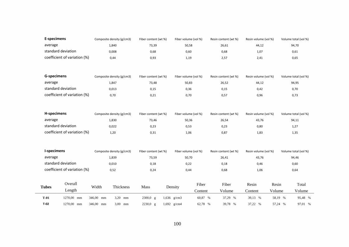
100
E-specimens Composite density (g/cm3)
Fiber content (wt %)
Fiber volume (vol %)
Resin content (wt %)
Resin volume (vol %)
Volume total (vol %)
average 1,840
73,39
50,58
26,61
44,12
94,70
standard deviation 0,008
0,68
0,60
0,68
1,07
0,61
coefficient of variation (%) 0,44
0,93
1,19
2,57
2,41
0,65
G-specimens Composite density (g/cm3)
Fiber content (wt %)
Fiber volume (vol %)
Resin content (wt %)
Resin volume (vol %)
Volume total (vol %)
average 1,847
73,48
50,83
26,52
44,12
94,95
standard deviation 0,013
0,15
0,36
0,15
0,42
0,70
coefficient of variation (%) 0,70
0,21
0,70
0,57
0,96
0,73
H-specimens Composite density (g/cm3)
Fiber content (wt %)
Fiber volume (vol %)
Resin content (wt %)
Resin volume (vol %)
Volume total (vol %)
average 1,830
73,46
50,36
26,54
43,76
94,11
standard deviation 0,022
0,23
0,53
0,23
0,80
1,27
coefficient of variation (%) 1,20
0,31
1,06
0,87
1,83
1,35
I-specimens Composite density (g/cm3)
Fiber content (wt %)
Fiber volume (vol %)
Resin content (wt %)
Resin volume (vol %)
Volume total (vol %)
average 1,839
73,59
50,70
26,41
43,76
94,46
standard deviation 0,010
0,18
0,22
0,18
0,46
0,60
coefficient of variation (%) 0,52
0,24
0,44
0,68
1,06
0,64
Tubes Overall
Width Thickness Mass Density Fiber Fiber Resin Resin Total Length Content Volume Content Volume Volume
T-01 1270,00 mm 346,00 mm 3,20 mm 2300,0 g 1,636 g/cm3 60,87 % 37,29 % 39,13 % 58,19 % 95,48 %
T-02 1270,00 mm 346,00 mm 3,00 mm 2230,0 g 1,692 g/cm4 62,78 % 39,78 % 37,22 % 57,24 % 97,01 %
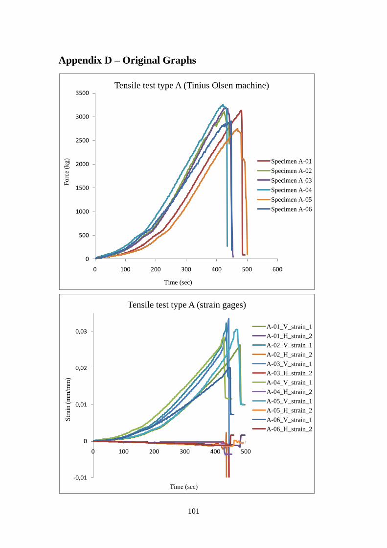
101
Appendix D – Original Graphs
0
500
1000
1500
2000
2500
3000
3500
0 100 200 300 400 500 600
Forc
e (k
g)
Time (sec)
Tensile test type A (Tinius Olsen machine)
Specimen A-01Specimen A-02Specimen A-03Specimen A-04Specimen A-05Specimen A-06
-0,01
0
0,01
0,02
0,03
0 100 200 300 400 500
Stra
in (m
m/m
m)
Time (sec)
Tensile test type A (strain gages)
A-01_V_strain_1A-01_H_strain_2A-02_V_strain_1A-02_H_strain_2A-03_V_strain_1A-03_H_strain_2A-04_V_strain_1A-04_H_strain_2A-05_V_strain_1A-05_H_strain_2A-06_V_strain_1A-06_H_strain_2
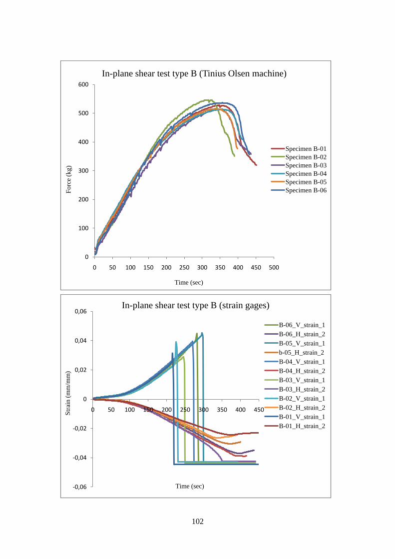
102
0
100
200
300
400
500
600
0 50 100 150 200 250 300 350 400 450 500
Forc
e (k
g)
Time (sec)
In-plane shear test type B (Tinius Olsen machine)
Specimen B-01Specimen B-02Specimen B-03Specimen B-04Specimen B-05Specimen B-06
-0,06
-0,04
-0,02
0
0,02
0,04
0,06
0 50 100 150 200 250 300 350 400 450Stra
in (m
m/m
m)
Time (sec)
In-plane shear test type B (strain gages)
B-06_V_strain_1B-06_H_strain_2B-05_V_strain_1b-05_H_strain_2B-04_V_strain_1B-04_H_strain_2B-03_V_strain_1B-03_H_strain_2B-02_V_strain_1B-02_H_strain_2B-01_V_strain_1B-01_H_strain_2
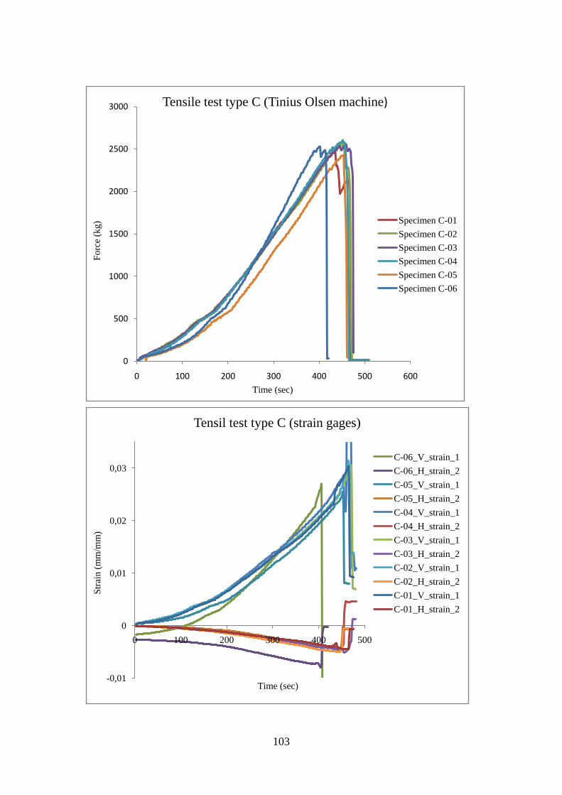
103
0
500
1000
1500
2000
2500
3000
0 100 200 300 400 500 600
Forc
e (k
g)
Time (sec)
Tensile test type C (Tinius Olsen machine)
Specimen C-01Specimen C-02Specimen C-03Specimen C-04Specimen C-05Specimen C-06
-0,01
0
0,01
0,02
0,03
0 100 200 300 400 500
Stra
in (m
m/m
m)
Time (sec)
Tensil test type C (strain gages)
C-06_V_strain_1C-06_H_strain_2C-05_V_strain_1C-05_H_strain_2C-04_V_strain_1C-04_H_strain_2C-03_V_strain_1C-03_H_strain_2C-02_V_strain_1C-02_H_strain_2C-01_V_strain_1C-01_H_strain_2
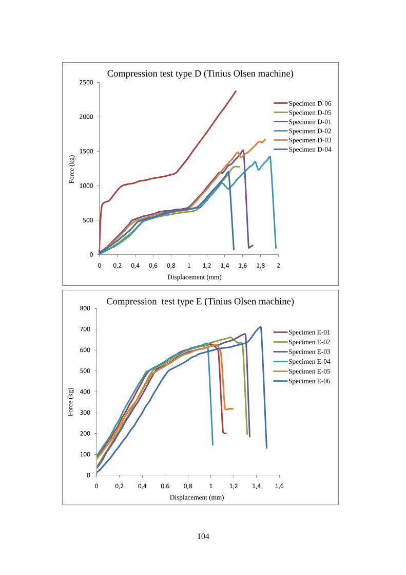
104
0
500
1000
1500
2000
2500
0 0,2 0,4 0,6 0,8 1 1,2 1,4 1,6 1,8 2
Forc
e (k
g)
Displacement (mm)
Compression test type D (Tinius Olsen machine)
Specimen D-06Specimen D-05Specimen D-01Specimen D-02Specimen D-03Specimen D-04
0
100
200
300
400
500
600
700
800
0 0,2 0,4 0,6 0,8 1 1,2 1,4 1,6
Forc
e (k
g)
Displacement (mm)
Compression test type E (Tinius Olsen machine)
Specimen E-01Specimen E-02Specimen E-03Specimen E-04Specimen E-05Specimen E-06
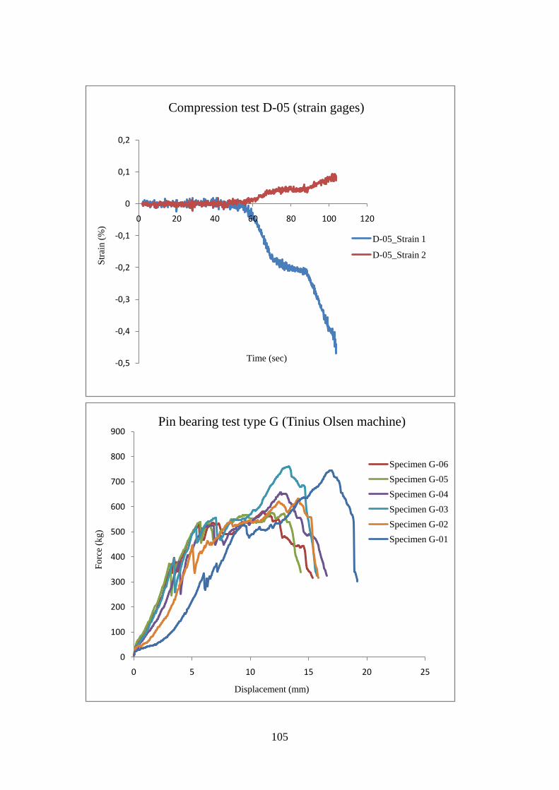
105
-0,5
-0,4
-0,3
-0,2
-0,1
0
0,1
0,2
0 20 40 60 80 100 120
Stra
in (%
)
Time (sec)
Compression test D-05 (strain gages)
D-05_Strain 1
D-05_Strain 2
0
100
200
300
400
500
600
700
800
900
0 5 10 15 20 25
Forc
e (k
g)
Displacement (mm)
Pin bearing test type G (Tinius Olsen machine)
Specimen G-06Specimen G-05Specimen G-04Specimen G-03Specimen G-02Specimen G-01
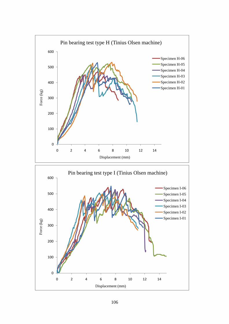
106
0
100
200
300
400
500
600
0 2 4 6 8 10 12 14
Forc
e (k
g)
Displacement (mm)
Pin bearing test type H (Tinius Olsen machine)
Specimen H-06Specimen H-05Specimen H-04Specimen H-03Specimen H-02Specimen H-01
0
100
200
300
400
500
600
0 2 4 6 8 10 12 14
Forc
e (k
g)
Displacement (mm)
Pin bearing test type I (Tinius Olsen machine)
Specimen I-06Specimen I-05Specimen I-04Specimen I-03Specimen I-02Specimen I-01
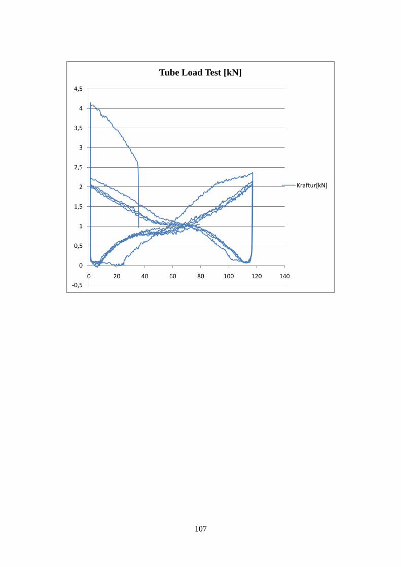
107
-0,5
0
0,5
1
1,5
2
2,5
3
3,5
4
4,5
0 20 40 60 80 100 120 140
Tube Load Test [kN]
Kraftur[kN]
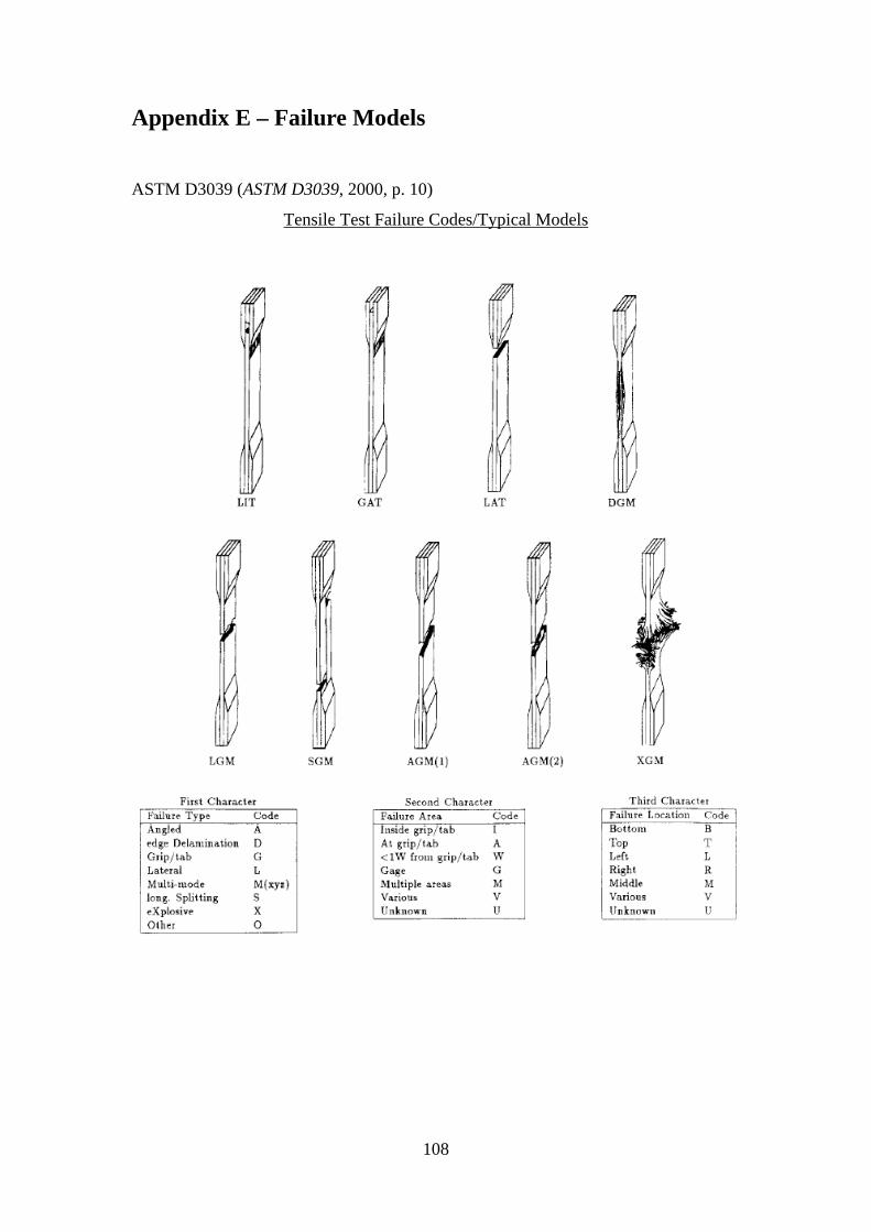
108
Appendix E – Failure Models
ASTM D3039 (ASTM D3039, 2000, p. 10)
Tensile Test Failure Codes/Typical Models
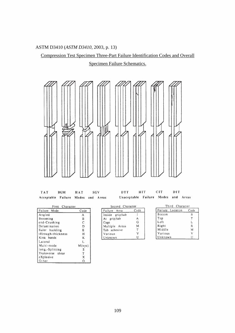
109
ASTM D3410 (ASTM D3410, 2003, p. 13)
Compression Test Specimen Three-Part Failure Identification Codes and Overall
Specimen Failure Schematics.
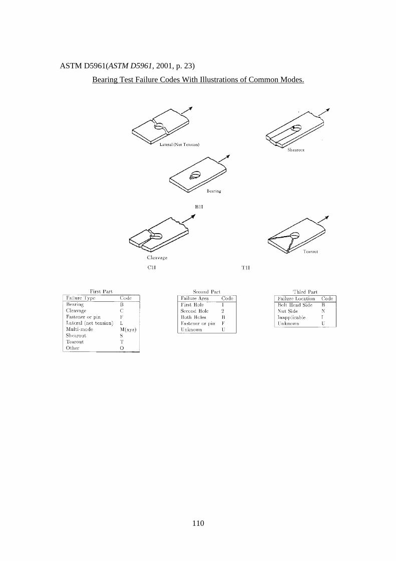
110
ASTM D5961(ASTM D5961, 2001, p. 23)
Bearing Test Failure Codes With Illustrations of Common Modes.
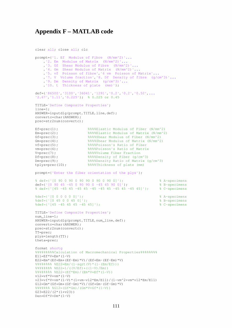
111
Appendix F – MATLAB code
clear all; close all; clc prompt={'1. Ef Modulus of Fibre (N/mm^2)'... ,'2. Em Modulus of Matrix (N/mm^2)'... ,'3. Gf Shear Modulus of Fibre (N/mm^2)'... ,'4. Gm Shear Modulus of Matrix (N/mm^2)'... ,'5. vf Poisson of fibre','6 vm Poisson of Matrix'... ,'7. V Volume fraction','8. Df Density of fibre (g/cm^3)'... ,'9. Dm Density of Matrix (g/cm^3)'... ,'10. t Thickness of plate (mm)'}; def={'86500','3100','36041','1291','0.2','0.2','0.52',... '2.67','1.11','0.225'}; % 0.225 or 0.45 TITLE='Define Composite Properties'; line=1; ANSWER=inputdlg(prompt,TITLE,line,def); convertc=char(ANSWER); prec=str2num(convertc); Ef=prec(1); %%%%Elastic Modulus of Fiber (N/mm^2) Em=prec(2); %%%%Elastic Modulus of Matrix (N/mm^2) Gf=prec(3); %%%%Shear Modulus of Fiber (N/mm^2) Gm=prec(4); %%%%Shear Modulus of Matrix (N/mm^2) vf=prec(5); %%%%Poisson's Ratio of Fiber vm=prec(6); %%%%Poisson's Ratio of Matrix V=prec(7); %%%%Volume Fiber Fraction Df=prec(8); %%%%Density of Fiber (g/cm^3) Dm=prec(9); %%%%Density Ratio of Matrix (g/cm^3) tplys=prec(10); %%%%Thickness of plate (mm) prompt={'Enter the fiber orientation of the plys'}; % def={'[0 90 0 90 0 90 90 0 90 0 90 0]'}; % A-specimens def={'[0 90 45 -45 0 90 90 0 -45 45 90 0]'}; % B-specimens % def={'[45 -45 45 -45 45 -45 -45 45 -45 45 -45 45]'}; % C-specimens %def={'[0 0 0 0 0 0]'}; % A-specimens %def={'[0 45 0 0 45 0]'}; % B-specimens %def={'[45 -45 45 45 -45 45]'}; % C-specimens TITLE='Define Composite Properties'; num_line=1; ANSWER=inputdlg(prompt,TITLE,num_line,def); convertc=char(ANSWER); prec=str2num(convertc); TT=prec; plys=length(TT); theta=prec; format shortg %%%%%%%%%Calculation of Macromechanical Properties%%%%%%%% E11=Ef*V+Em*(1-V) E22=Em*(Ef+Em+(Ef-Em)*V)/(Ef+Em-(Ef-Em)*V) %%%%%%%% %E22=Em/(1-sqrt(V)*(1-(Em/Ef))) %%%%%%%% %E22=1/((V/Ef)+((1-V)/Em)) %%%%%%%% %E22=(Ef*Em)/(Em*V+Ef*(1-V)) v12=vf*V+vm*(1-V) v23=vf*V+vm*(1-V)*(1+vm-v12*Em/E11)/(1-vm^2+vm*v12*Em/E11) G12=Gm*(Gf+Gm+(Gf-Gm)*V)/(Gf+Gm-(Gf-Gm)*V) %%%%%%% %G12=(Gf*Gm)/(Gm*V+Gf*(1-V)) G23=E22/(2*(1+v23)) Den=Df*V+Dm*(1-V)
112
E1=E11; E2=E22; %%%%%% %E2=1; %%%%%%%%%%%%%%%%%%%%%%%%%%%%%%%%%%%%%%%%%%%%%%%%%%%%%%%%%%% %%%%%%%%%%%%%%%%%%%%%%%%%%%%%%%%%%%%%%%%%%%%%%%%%%%%%%%%%%% % E1=19817; % E2=19817; % v12=0.054; % G12=2750; %%%%%%%%%%%%%%%%%%%%%%%%%%%%%%%%%%%%%%%%%%%%%%%%%%%%%%%%%% %% t(1:plys)=tplys; for i = 1:plys [Q,S,Qbar(:,:,i),Sbar(:,:,i),T(:,:,i)]=qands(E1,E2,G12,v12,theta(i)); end [ABD,z,z0] = abd(t,Qbar,plys); %% % e0_K=[ex ey exy Kx Ky Kxy]' % e0_K=[0.03 -0.005 0 0 0 0]; % N_M=(ABD*e0_K')' %% %N_M=[35000/25 0 0 0 0 0]; % A-specimens %N_M=[5000/25 0 0 0 0 0]; % B-specimens N_M=[9000/25 0 0 0 0 0]; % C-specimens e0_K = inv(ABD)*N_M'; e0(:,1) = e0_K(1:3); K(:,1) = e0_K(4:6); %% %************************* % GENERATES ALL Ex, Ey,exy %************************* xstrain(1,1)=e0(1)+z0*K(1); ystrain(1,1)=e0(2)+z0*K(2); xystrain(1,1)=e0(3)+z0*K(3); for i = 2:plys+1 xstrain(i,1)=e0(1)+z(i-1)*K(1); ystrain(i,1)=e0(2)+z(i-1)*K(2); xystrain(i,1)=e0(3)+z(i-1)*K(3); if abs(xystrain) < 1e-9 xystrain(i,1)=0; end end for i = 1:plys+1 e(:,i)=[xstrain(i,1);ystrain(i,1);xystrain(i,1)]; end %************************************* % GENERATES ALL Global & Ply stresses %************************************* for i = 1:plys globalstresses(1:3,i)=Qbar(:,:,i)*e(:,i); globalstresses(4:6,i)=Qbar(:,:,i)*e(:,(i+1)); plystresses(1:3,i)=T(:,:,i)*globalstresses(1:3,i); plystresses(4:6,i)=T(:,:,i)*globalstresses(4:6,i); end
113
%% Material strengths sigma_1C = -300; % Compression failure stress in the 1 direction (N/mm^2) sigma_1T = 900; % Tensile failure stress in the 1 direction (N/mm^2) sigma_2C = -100; % Compression failure stress in the 2 direction (N/mm^2) sigma_2T = 49.5; % Tensile failure stress in the 2 direction (N/mm^2) tau_F12 = 38; % Shear failure stress in the 1-2 plan (N/mm^2) plystresses; %% Maximum Stress Theory--------------------------------------------------- StressFailure=zeros(3,plys); for i = 1:plys if plystresses(1,i) >= 0; StressFailure(1,i)=plystresses(1,i)/sigma_1T; else StressFailure(1,i)=plystresses(1,i)/sigma_1C; end if plystresses(2,i) >= 0; StressFailure(2,i)=plystresses(2,i)/sigma_2T; else StressFailure(2,i)=plystresses(2,i)/sigma_2C; end StressFailure(3,i)=abs(plystresses(3,i))/tau_F12; end StressFailure; for i = 1:plys StressFailureMax(:,i)=max(abs(StressFailure(:,i))); end StressFailureMax; %% Maximum Strain Theory--------------------------------------------------- % strain_local=zeros(3,plys); strain_local(1,:)=(plystresses(1,:))./E1-(v12.*plystresses(2,:))./E1; strain_local(2,:)=(plystresses(2,:))./E2-(v12.*plystresses(1,:))./E1; strain_local(3,:)=(plystresses(3,:))./G12; epsilon_1C = sigma_1C/E1; epsilon_1T = sigma_1T/E1; epsilon_2C = sigma_2C/E2; epsilon_2T = sigma_2T/E2; gamma_F12 = tau_F12/G12; StrainFailure=zeros(3,plys); for i = 1:plys if strain_local(1,i) >= 0; StrainFailure(1,i)=strain_local(1,i)./epsilon_1T; else StrainFailure(1,i)=strain_local(1,i)./epsilon_1C; end if strain_local(2,i) >= 0; StrainFailure(2,i)=strain_local(2,i)./epsilon_2T; else StrainFailure(2,i)=strain_local(2,i)./epsilon_2C; end StrainFailure(3,i)=abs(strain_local(3,i))./gamma_F12; end StrainFailure; for i = 1:plys StrainFailureMax(:,i)=max(abs(StrainFailure(:,i))); end StrainFailureMax;

114
%% Tsai-Hill (Maximum Work) Theory (if sigma_1C = sigma_1T) for i = 1:plys if plystresses(1,i) >= 0; if plystresses(2,i) >= 0; Tsai_Hill(1,i) = (plystresses(1,i)^2/sigma_1T^2)+(plystresses(2,i)... ^2/sigma_2T^2)-((plystresses(1,i)*plystresses(2,i))/sigma_1T^2)+... (plystresses(3,i)^2/tau_F12^2); else Tsai_Hill(1,i) = (plystresses(1,i)^2/sigma_1T^2)+(plystresses(2,i)... ^2/sigma_2C^2)-((plystresses(1,i)*plystresses(2,i))/sigma_1T^2)+... (plystresses(3,i)^2/tau_F12^2); end else if plystresses(2,i) >= 0; Tsai_Hill(1,i) = (plystresses(1,i)^2/sigma_1C^2)+(plystresses(2,i)... ^2/sigma_2T^2)-((plystresses(1,i)*plystresses(2,i))/sigma_1C^2)+... (plystresses(3,i)^2/tau_F12^2); else Tsai_Hill(1,i) = (plystresses(1,i)^2/sigma_1C^2)+(plystresses(2,i)... ^2/sigma_2C^2)-((plystresses(1,i)*plystresses(2,i))/sigma_1C^2)+... (plystresses(3,i)^2/tau_F12^2); end end end Tsai_Hill; %% Tsai-Wu Theory f1=(1/sigma_1T)+(1/sigma_1C); f11=-(1/(sigma_1T*sigma_1C)); f2=(1/sigma_2T)+(1/sigma_2C); f22=-(1/(sigma_2T*sigma_2C)); f66=(1/tau_F12)^2; %f12=-(1/2)*(1/(sigma_1T*sigma_1C*sigma_2T*sigma_2C))^0.5; for i = 1:plys Tsai_Wu(1,i)=f1*plystresses(1,i)+f2*plystresses(2,i)+... f11*plystresses(1,i)^2+f22*plystresses(2,i)^2+f66*plystresses(3,i)... ^2-(f11*f22)^2*plystresses(1,i)*plystresses(2,i); end Tsai_Wu;
115
%CALCULATES Q,Qbar, S, Sbar MATRICIES % function [Q,S,Qbar,Sbar,T]=qands(E1,E2,G12,v12,theta) theta = theta*pi/180; c = cos(theta); s = sin(theta); R = [1 0 0;0 1 0;0 0 2]; %Rueter Transformation Matrix T = [c^2 s^2 2*c*s;s^2 c^2 -2*c*s; -c*s c*s c^2-s^2];%Transformation Matrix %**************** %Formulation of S %**************** S11 = 1/E1; S22 = 1/E2; S66 = 1/G12; S12 = -v12/E1; S21 = S12; S = [S11,S12,0;S21,S22,0;0,0,S66]; %**************** %Formulation of Q %**************** Q = S^-1; %**************************** %Formulation of Q-BAR & S-BAR %**************************** Qbar = (T^-1)*Q*R*T*(R^-1); Sbar = R*(T^-1)*(R^-1)*S*T; %Sub Program: ABD Assemblage
% CALCULATES THE ABD MATRIX OF THE PANEL function [ABD,z,z0]=abd(t,Qbar,plys); z0 = -sum(t)/2; z(1) = z0+t(1); % cant use a zeroth row... so notation is offset by 1 number .. % for technically z_1 to z_(n+1) (same # of points) for j = 2:plys z(j)=z(j-1)+t(j); end for i = 1:3 for j = 1:3 A(i,j) = Qbar(i,j,1)*(z(1)-z0); B(i,j) = Qbar(i,j,1)*(z(1)^2-z0^2)/2; D(i,j) = Qbar(i,j,1)*(z(1)^3-z0^3)/3; for k = 2:plys A(i,j) = A(i,j)+Qbar(i,j,k)*(z(k)-z(k-1)); B(i,j) = B(i,j)+Qbar(i,j,k)*(z(k)^2-z(k-1)^2)/2; D(i,j) = D(i,j)+Qbar(i,j,k)*(z(k)^3-z(k-1)^3)/3; end end end ABD = [A,B;B,D];
116
% PLOTTING FUNCTION %************************************************* % Plots and displays all needed values %************************************************* function [thickness,strainthickness] = graphics(z,z0,plys,globalstresses,... plystresses,xstrain,ystrain,xystrain,sigma_1C,sigma_2C,sigma_1T,... sigma_2T,tau_F12,strain_local,epsilon_1C,epsilon_1T,epsilon_2C,... epsilon_2T,gamma_F12); %********************************************************************** % sorts all stress/strains so they can be plotted %********************************************************************** j=1; for i = 1:2:(plys*2-1) sigx(i)=globalstresses(1,j); sigx(i+1)=globalstresses(4,j); sigy(i)=globalstresses(2,j); sigy(i+1)=globalstresses(5,j); sigxy(i)=globalstresses(3,j); sigxy(i+1)=globalstresses(6,j); sig1(i)=plystresses(1,j); sig1(i+1)=plystresses(4,j); sig2(i)=plystresses(2,j); sig2(i+1)=plystresses(5,j); sig12(i)=plystresses(3,j); sig12(i+1)=plystresses(6,j); str1(i)=strain_local(1,j); str1(i+1)=strain_local(1,j); str2(i)=strain_local(2,j); str2(i+1)=strain_local(2,j); str12(i)=strain_local(3,j); str12(i+1)=strain_local(3,j); j=j+1; end %********************************************************************** % Generates all thicknesses so that they can be plotted against the stresses/strains %********************************************************************** thickness(1)=z0; strainthickness(1)=z0; m=2; for i = 1:plys thickness(m)=z(i); thickness(m+1)=z(i); m=m+2; end [m,n]=size(thickness); thickness=thickness(1:(n-1)); m=2; for i = 1:plys strainthickness(m)=z(i); m=m+1; end strainthickness; clc format shortg labelfor={'fontname','times new roman','fontsize',12}; figure(1);plot(sigx,thickness,'b-') legend('Stress x',0);ylabel('Thickness (mm)',labelfor{:});xlabel('Stress (MPa)',labelfor{:}); %title('Stress through the thickness in the (X,Y) global coordinate system') figure(2);plot(sigy,thickness,'b-') legend('Stress y',0);ylabel('Thickness(mm)',labelfor{:});xlabel('Stress(MPa)',labelfor{:}); %title('Stress through the thickness in the (X,Y) global coordinate system')

117
figure(3);plot(sigxy,thickness,'b-') legend('Shear stress xy',0);ylabel('Thickness(mm)',labelfor{:});xlabel('Stress(MPa)',labelfor{:}); %title('Stress through the thickness in the (X,Y) global coordinate system') figure(4);plot(sig1,thickness,'b-') hold on; plot([sigma_1C sigma_1C],[thickness(1) thickness(length(thickness))],'r','LineWidth',2); plot([sigma_1T sigma_1T],[thickness(1) thickness(length(thickness))],'r','LineWidth',2); %axis([sigma_1C-10 sigma_1T+10 thickness(1) thickness(length(thickness))]); legend('Stress 1','Maximum Stress');ylabel('Thickness(mm)',labelfor{:});xlabel('Stress(MPa)',labelfor{:}); %title('Stress through the thickness in the (1,2) local coordinate system') figure(5);plot(sig2,thickness,'b-'); hold on; plot([sigma_2C sigma_2C],[thickness(1) thickness(length(thickness))],'r','LineWidth',2); plot([sigma_2T sigma_2T],[thickness(1) thickness(length(thickness))],'r','LineWidth',2); %axis([sigma_2C-10 sigma_2T+10 thickness(1) thickness(length(thickness))]); legend('Stress 2','Maximum Stress');ylabel('Thickness(mm)',labelfor{:});xlabel('Stress(MPa)',labelfor{:}); %title('Stress through the thickness in the (1,2) local coordinate system') figure(6);plot(sig12,thickness,'b-') hold on; plot([tau_F12 tau_F12],[thickness(1) thickness(length(thickness))],'r','LineWidth',2); plot([-tau_F12 -tau_F12],[thickness(1) thickness(length(thickness))],'r','LineWidth',2); %axis([-tau_F12-10 tau_F12+10 thickness(1) thickness(length(thickness))]); legend('Shear stress 12','Maximum Stress');ylabel('Thickness(mm)',labelfor{:});xlabel('Stress(MPa)',labelfor{:}); %title('Stress through the thickness in the (L,T) local coordinate system') figure(7);plot(xstrain,strainthickness,'b-') axis([-0.01 0.04 -1.5 1.5]) legend('Strain x',0);ylabel('Thickness(mm)',labelfor{:});xlabel('Strain (mm/mm)',labelfor{:}); %title('Strain through the thickness in the (X,Y) global coordinate system') figure(8);plot(ystrain,strainthickness,'b-') axis([-0.01 0.04 -1.5 1.5]) legend('Strain y',0);ylabel('Thickness(mm)',labelfor{:});xlabel('Strain (mm/mm)',labelfor{:}); %title('Strain through the thickness in the (X,Y) global coordinate system') figure(9);plot(xystrain,strainthickness,'b-') axis([-0.01 0.04 -1.5 1.5]) legend('Shear strain xy',0);ylabel('Thickness(mm)',labelfor{:});xlabel('Strain (mm/mm)',labelfor{:}); %title('Strain through the thickness in the (X,Y) global coordinate system') figure(10);plot(str1,thickness,'b-') hold on; plot([epsilon_1C epsilon_1C],[thickness(1) thickness(length(thickness))],'r','LineWidth',2); plot([epsilon_1T epsilon_1T],[thickness(1) thickness(length(thickness))],'r','LineWidth',2); %axis([sigma_1C-10 sigma_1T+10 thickness(1) thickness(length(thickness))]); legend('Strain 1','Maximum Strain');ylabel('Thickness(mm)',labelfor{:});xlabel('Strain(mm/mm)',labelfor{:}); %title('Strain through the thickness in the (L,T) local coordinate system') figure(11);plot(str2,thickness,'b-') hold on; plot([epsilon_2C epsilon_2C],[thickness(1) thickness(length(thickness))],'r','LineWidth',2); plot([epsilon_2T epsilon_2T],[thickness(1) thickness(length(thickness))],'r','LineWidth',2); %axis([sigma_1C-10 sigma_1T+10 thickness(1) thickness(length(thickness))]); legend('Strain 2','Maximum Strain');ylabel('Thickness(mm)',labelfor{:});xlabel('Strain(mm/mm)',labelfor{:}); %title('Strain through the thickness in the (L,T) local coordinate system')

118
figure(12);plot(str12,thickness,'b-') hold on; plot([epsilon_2C epsilon_2C],[thickness(1) thickness(length(thickness))],'r','LineWidth',2); plot([gamma_F12 gamma_F12],[thickness(1) thickness(length(thickness))],'r','LineWidth',2); %axis([sigma_1C-10 sigma_1T+10 thickness(1) thickness(length(thickness))]); legend('Shear strain 12','Maximum Strain');ylabel('Thickness(mm)',labelfor{:});xlabel('Strain(mm/mm)',labelfor{:}); %title('Strain through the thickness in the (L,T) local coordinate system')

119
Appendix G – Videos of the experiments (DVD)