contents 1.motivation for nonlinear controlmotivation for nonlinear control 2.the tracking...
TRANSCRIPT
Contents1. Motivation for Nonlinear Control2. The Tracking Problem
1. Feedback Linearization3. Adaptive Control4. Robust Control
1. Sliding mode2. High-gain3. High-frequency
5. Learning Control6. The Tracking Problem, Revisited Using the Desired Trajectory
1. Feedback Linearization2. Adaptive Control
7. Filtered tracking error r(t) for second-order systems)8. Introduction to Observers9. Observers + Controllers10. Filter Based Control
1. Filter + Adaptive Control11. Summary
12. Homework Problems1. A12. A23. A34. A4 – Design observer, observer + controller, control based on filter
2
Nonlinear Control
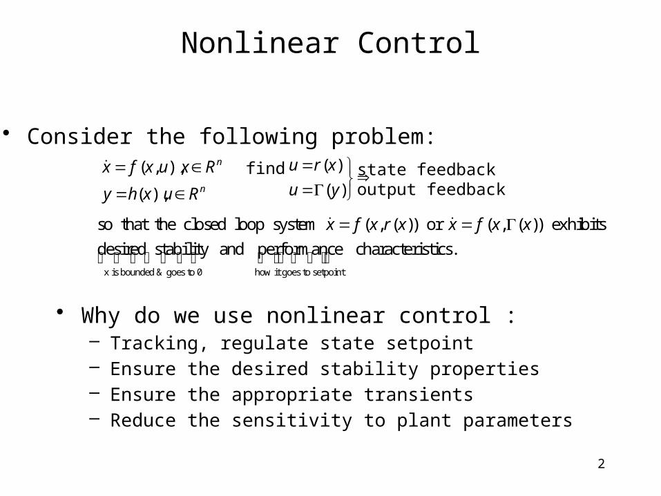
• Why do we use nonlinear control :– Tracking, regulate state setpoint– Ensure the desired stability properties– Ensure the appropriate transients– Reduce the sensitivity to plant parameters
find ( )
( )
u r x
u y
state feedbackoutput feedback
• Consider the following problem:
x is bounded & goes to 0 how it goes to setpoint
so that the closed loop system ( , ( )) or ( , ( )) exhibits
desired stability and performance characteristics.
x f x r x x f x x
n
n
Ruxhy
Rxuxfx
),(
),,(

Applications and Areas of Interest
Mobile Platforms
• UUV, UAV, and UGV• Satellites & Aircraft
Automotive Systems
• Steer-By-Wire• Thermal Management• Hydraulic Actuators• Spark Ignition• CVT
Mechanical Systems
• Textile and Paper Handling• Overhead Cranes• Flexible Beams and Cables• MEMS Gyros
Robotics
• Position/Force Control • Redundant and Dual Robots• Path Planning• Fault Detection• Teleoperation and Haptics
Electrical/Computer Systems
• Electric Motors• Magnetic Bearings• Visual Servoing• Structure from Motion
Nonlinear Control and Estimation Chemical Systems
• Bioreactors• Tumor Modeling
The Mathematical Problem
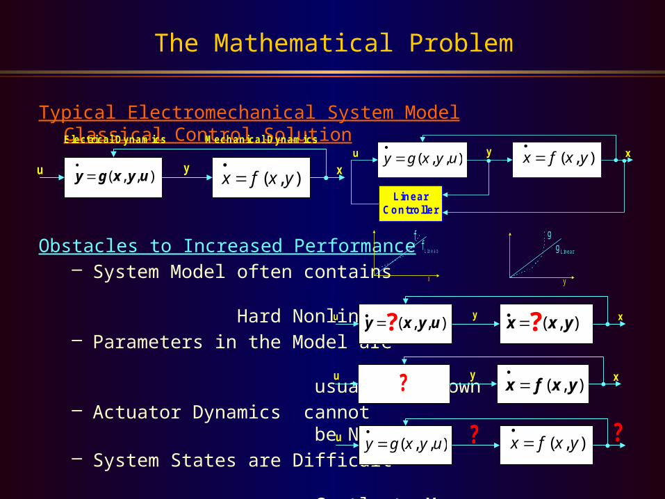
Typical Electromechanical System Model Classical Control Solution
Obstacles to Increased Performance– System Model often contains
Hard Nonlinearities– Parameters in the Model are
usually Unknown– Actuator Dynamics cannot
be Neglected– System States are Difficult
or Costly to Measure
x f x y·
( , )y g x y u·
( , , )u y x
Electrical Dynamics Mechanical Dynamics
x f x y·
( , )y g x y u·
( , , )u y x
LinearController
fLinear
f
x
gLinear
g
y
u y xy x y u· ?( , , ) x x y
· ?( , )
x f x y·
( , )?u y x
x f x y·
( , )y g x y u·
( , , )u ? ?
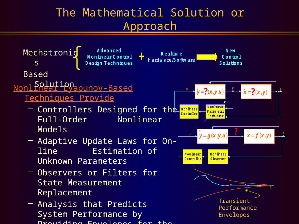
Nonlinear Lyapunov-Based Techniques Provide– Controllers Designed for the Full-Order
Nonlinear Models– Adaptive Update Laws for On-line
Estimation of Unknown Parameters– Observers or Filters for State
Measurement Replacement– Analysis that Predicts System
Performance by Providing Envelopes for the Transient Response
The Mathematical Solution or Approach
Mechatronics
Based Solution
AdvancedNonlinear Control
Design Techniques
RealtimeHardw are/Softw are+
NewControl
Solutions
u y x
NonlinearParameterEstimator
NonlinearController
y x y u· ?( , , ) x x y
· ?( , )
x f x y·
( , )y g x y u·
( , , )u ? x
NonlinearObserver
NonlinearController
t
Transient Performance Envelopes
6
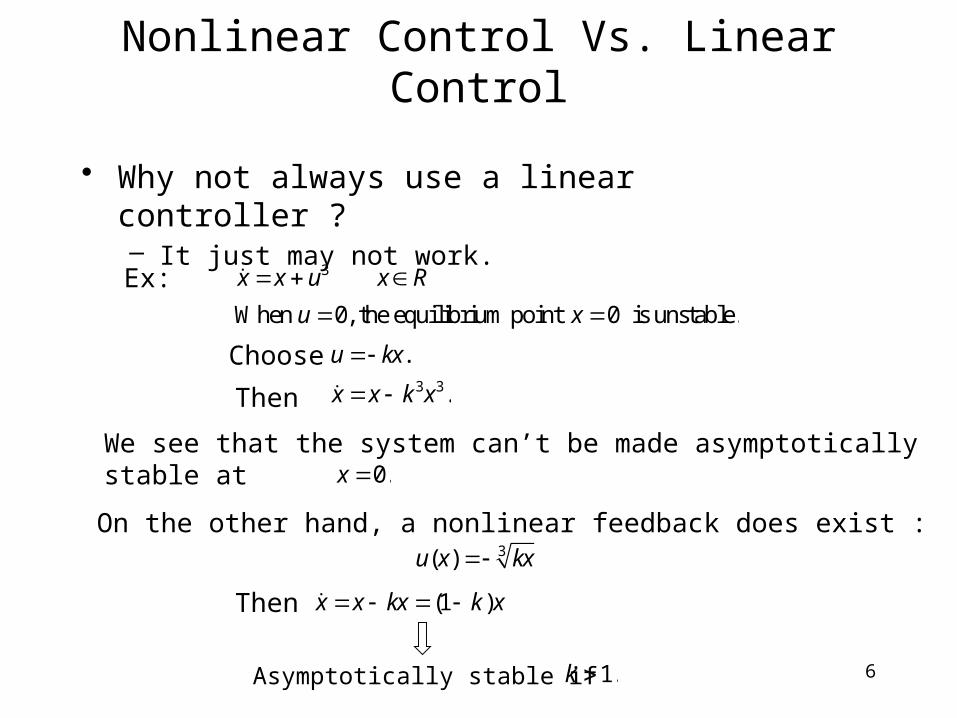
Nonlinear Control Vs. Linear Control
• Why not always use a linear controller ?– It just may not work.
Ex: 3x x u x R
When 0, the equilibrium point 0 is unstable.u x
Choose3 3
.
.
u kx
x x k x
We see that the system can’t be made asymptotically stable at 0.x
On the other hand, a nonlinear feedback does exist :3( )u x kx
Then (1 )x x kx k x
Asymptotically stable if 1.k
Then
7
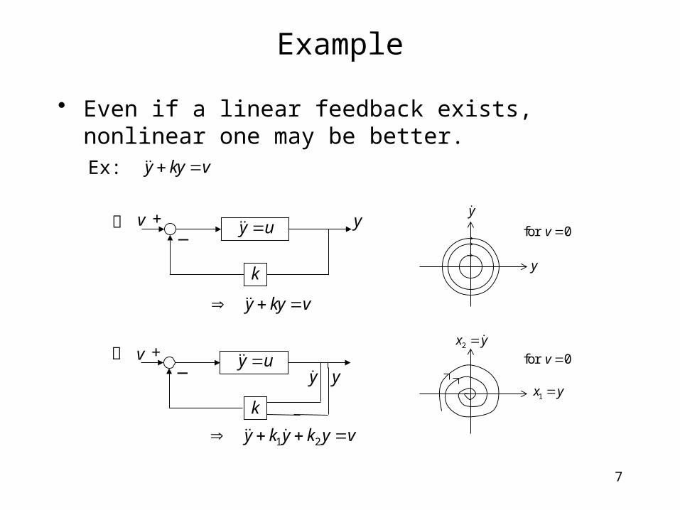
Example
• Even if a linear feedback exists, nonlinear one may be better.Ex: y ky v
y u
k
+_
v y
y u+_
vy
k
y
1 2y k y k y v
y ky v
for 0v
y
y
1x y
2x yfor 0v
8
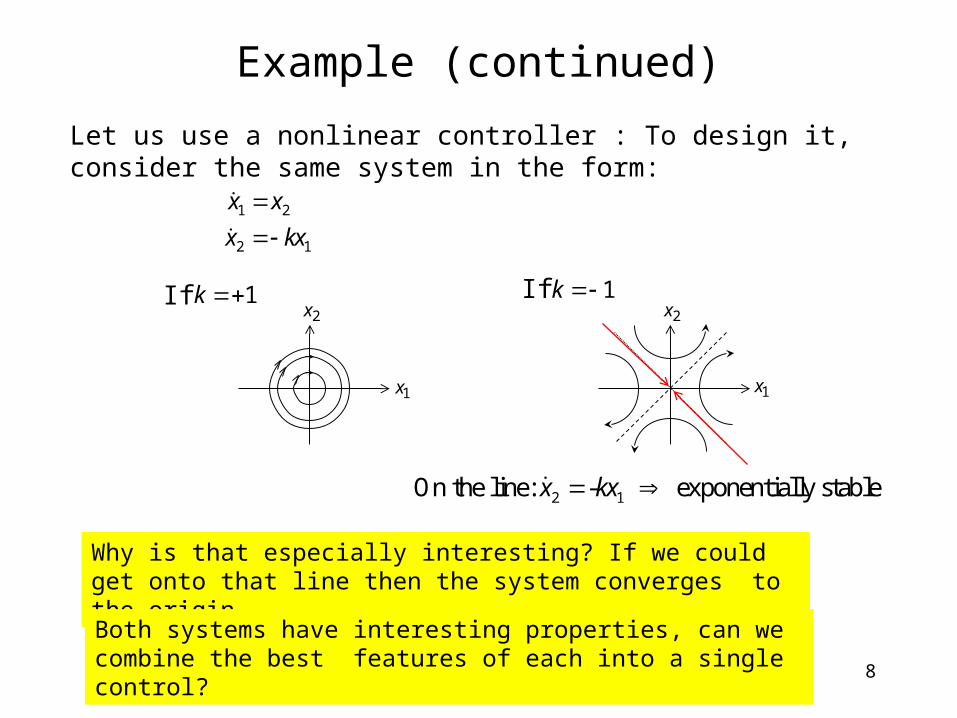
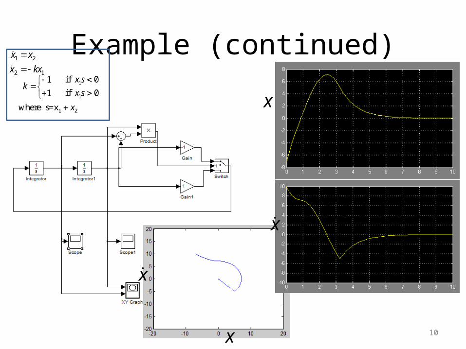
Example (continued)
Let us use a nonlinear controller : To design it, consider the same system in the form:
1 2
2 1
x x
x kx
If 1k If 1k
1x
2x
1x
2x
2 1On the line: - exponentially stablex kx
Why is that especially interesting? If we could get onto that line then the system converges to the origin
Both systems have interesting properties, can we combine the best features of each into a single control?
9
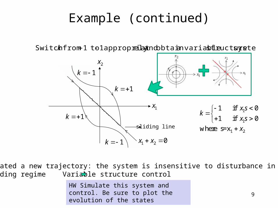
Example (continued)
1x
2x
1 2 0x x
1k
1k
1k
1k
sliding line
1
1
if 01
if 01
x sk
x s
1 2where s=x x
Created a new trajectory: the system is insensitive to disturbance in thesliding regime Variable structure control
system. structure variableaobtain andely appropriat 1 to1 from Switch k
HW Simulate this system and control. Be sure to plot the evolution of the states
Example (continued)
10
x
x
x
x
1 2
2 1
x x
x kx
1
1
if 01
if 01
x sk
x s
1 2where s=x x
11
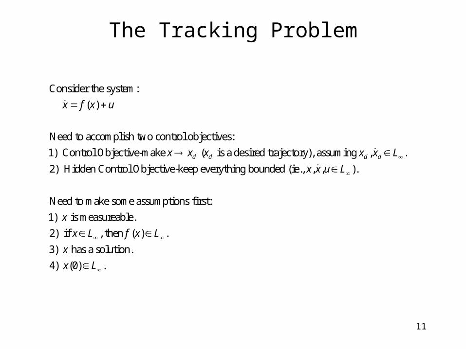
Consider the system:
( )
Need to accomplish two control objectives:
1) Control Objective-make ( is a desired trajectory), assuming , .
2) Hidden Control Objective-keep everythind d d d
x f x u
x x x x x L
g bounded (ie., , , ).
Need to make some assumptions first:
1) is measureable.
2) if , then ( ) .
3) has a solution.
4) (0) .
x x u L
x
x L f x L
x
x L
The Tracking Problem
12
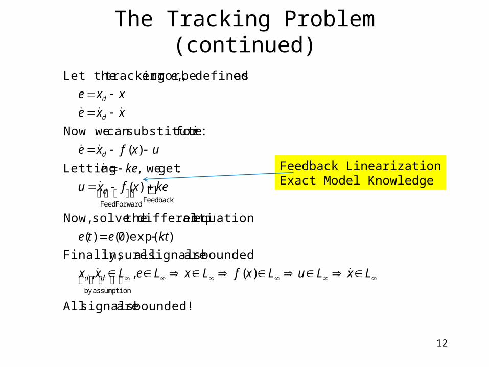
The Tracking Problem (continued)
bounded! are signals All
)( ,,
bounded are signals all insure Finally,
)exp()0()(
equation aldifferenti thesolve Now,
)(
:get we, Letting
)(
:for substitutecan weNow
as defined be , error, trackingLet the
assumptionby
FeedbackForward Feed
LxLuLxfLxLeLxx
ktete
kexfxu
kee
uxfxe
x
xxe
xxe
e
dd
d
d
d
d
Feedback LinearizationExact Model Knowledge
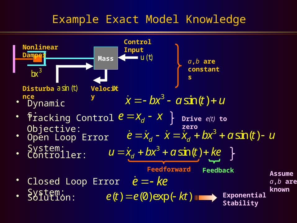
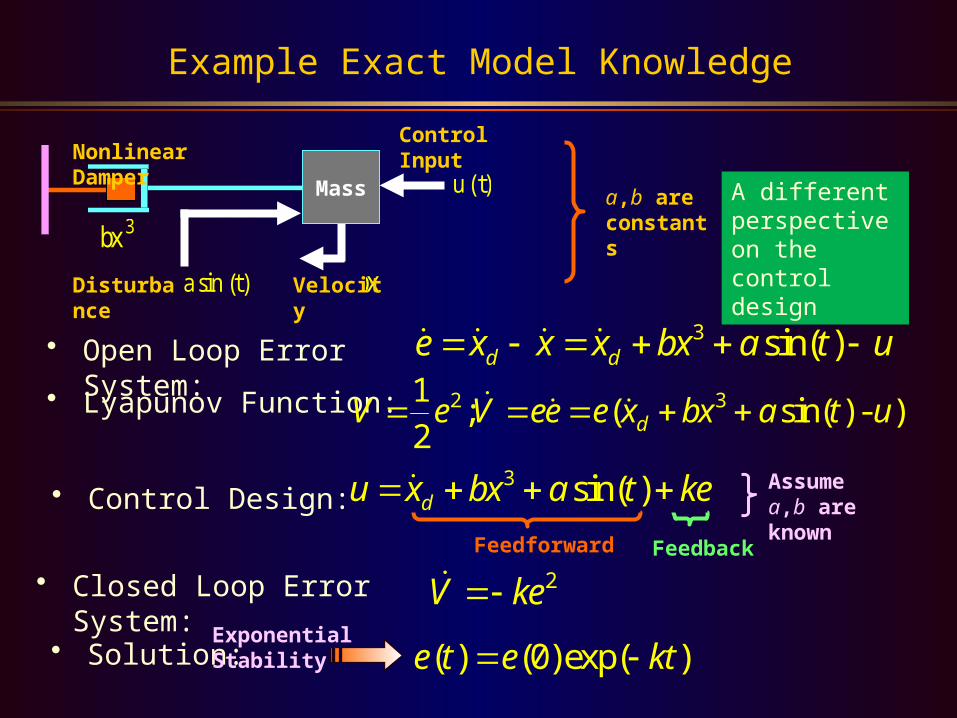
Example Exact Model Knowledge
• Dynamics:
Mass
bx3
asin(t) bx3
u(t)Nonlinear Damper
Disturbance Velocity
Control Input
a,b are constants
• Tracking Control Objective:
• Open Loop Error System:
• Controller:
• Closed Loop Error System:
• Solution:
Feedforward Feedback Assume a,b are known
Drive e(t) to zero
Exponential Stability
3 sin( )x bx a t u
de x x 3 sin( )d de x x x bx a t u
3 sin( )du x bx a t ke
e ke( ) (0)exp( )e t e kt
Example Exact Model Knowledge
Mass
bx3
asin(t) bx3
u(t)Nonlinear Damper
Disturbance Velocity
Control Input
a,b are constants
• Open Loop Error System:
• Control Design:
• Closed Loop Error System:
• Solution:
Feedforward Feedback
Assume a,b are known
Exponential Stability
3 sin( )d de x x x bx a t u
3 sin( )du x bx a t ke
( ) (0)exp( )e t e kt
• Lyapunov Function: 2 31; ( sin( ) - )
2 dV e V ee e x bx a t u
2V ke
A different perspective on the control design
15
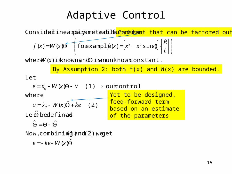
Adaptive Control
~)(
get we(2), and (1) combining Now,
ˆ~
as defined be ~
Let
(2) ˆ)(
where
controlour (1) )(
Let
constant.unknown an is and known, is )( where
)sin( )( examplefor )()(
function zableparameterilinearily aConsider
32
xWkee
kexWxu
uxWxe
xW
L
RxxxxfxWxf
d
d
By Assumption 2: both f(x) and W(x) are bounded.
Constant that can be factored out
Yet to be designed, feed-forward term based on an estimate of the parameters
16
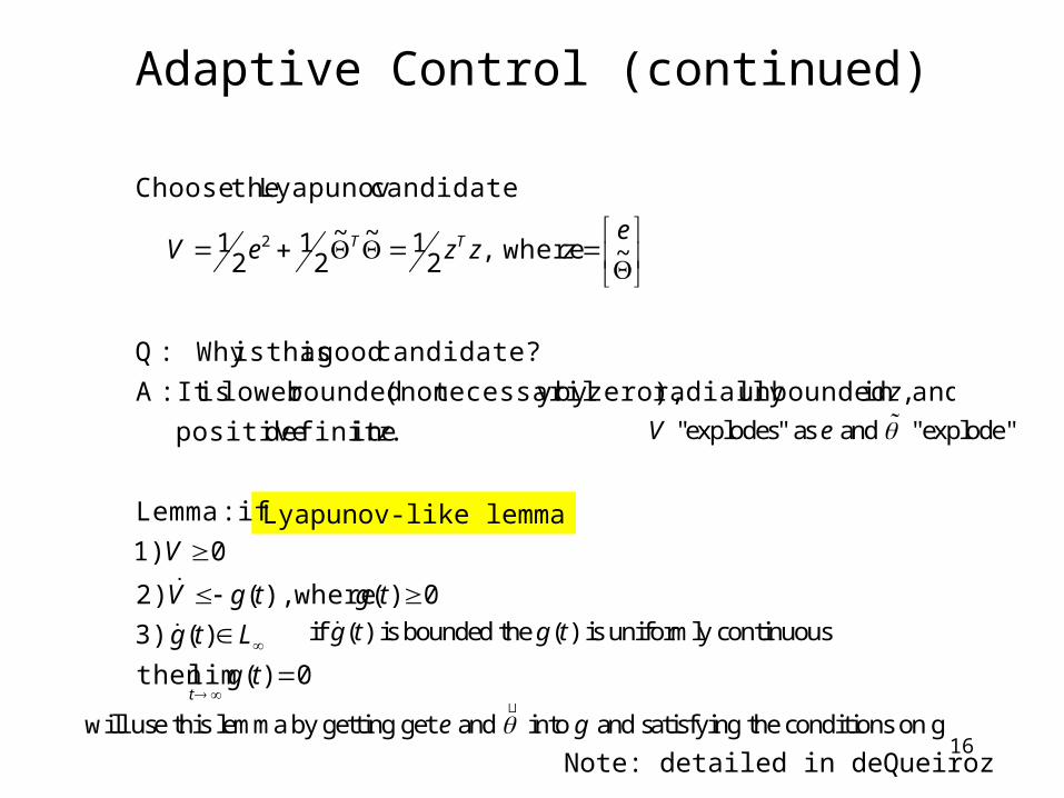
Adaptive Control (continued)
0)(limthen
)( 3)
0)( where),( 2)
0 1)
if :Lemma
.in definite positive
and ,in unboundedradially zero),by y necessaril(not boundedlower isIt :A
candidate? good a thisis Why :Q
~ where,21~~
21
21
candidate Lyapunov theChoose
2
tg
Ltg
tgtgV
V
z
z
ezzzeV
t
TT
Lyapunov-like lemma
if ( ) is bounded the ( ) is uniformly continuousg t g t
Note: detailed in deQueirozwill use this lemma by getting get and into and satisfying the conditions on ge g
"explodes" as and "explode"V e
17
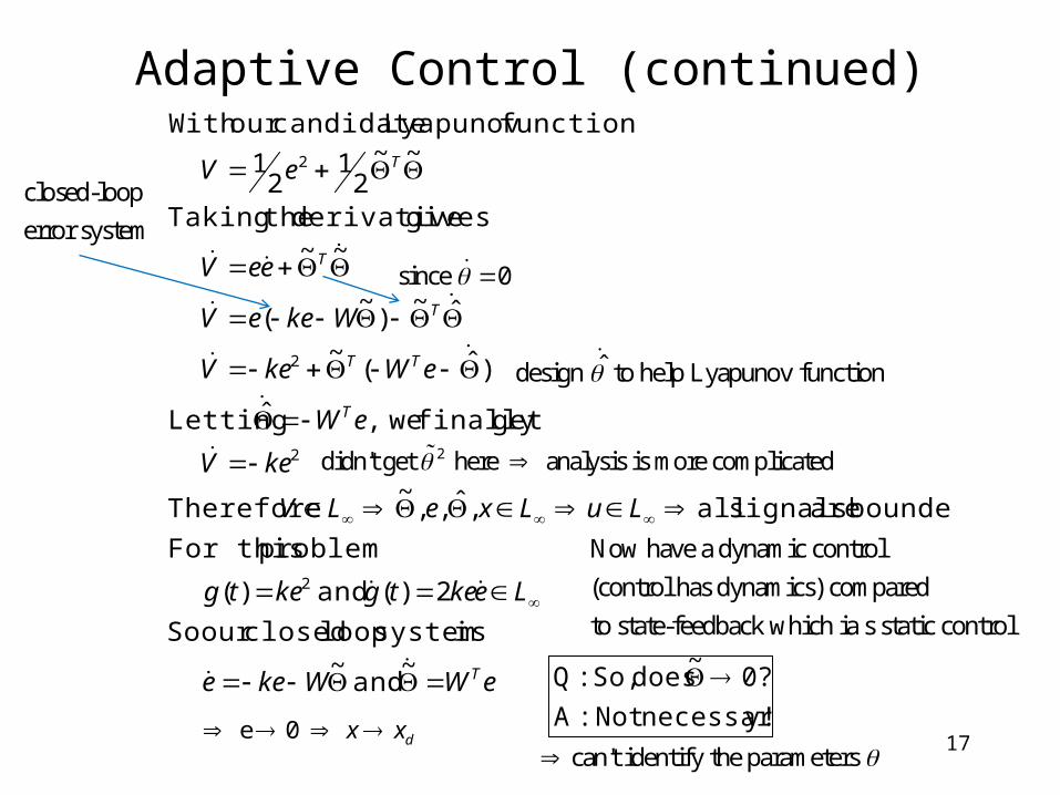
eWWkee
Leketgketg
LuLxeLV
keV
eW
eWkeV
WkeeV
eeV
eV
T
T
TT
T
T
T
~ and
~
is system loop closedour So
2)( and )(
problem For this
bounded! are signals all,ˆ,,~
Therefore
getfinally we,ˆ Letting
)ˆ(~
ˆ~)
~(
~~
gives derivative theTaking
~~2
12
1
function Lyapunov candidateour With
2
2
2
2
y!necessarilNot :A
?0~
does So, :Q
Adaptive Control (continued)
closed-loop
error system
since 0
ˆdesign to help Lyapunov function
can't identify the parameters
2didn't get here analysis is more complicated
e 0 dx x
Now have a dynamic control
(control has dynamics) compared
to state-feedback which ia s static control
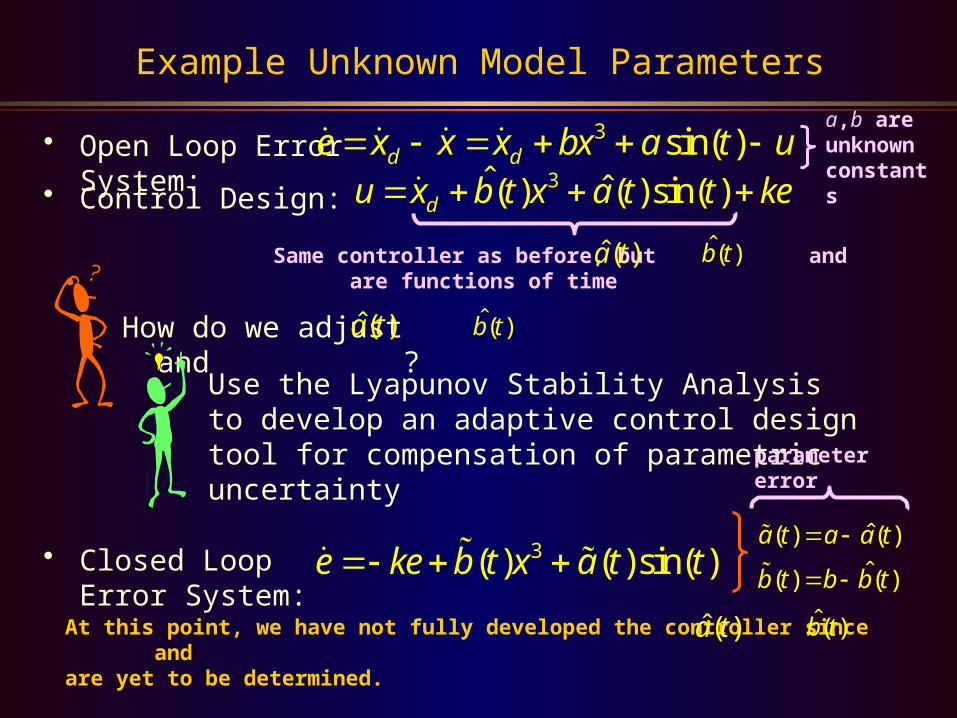
Example Unknown Model Parameters
• Open Loop Error System:• Control Design:
a,b are unknownconstants
Same controller as before, but and are functions of time
How do we adjust and ?
Use the Lyapunov Stability Analysis to develop an adaptive control design tool for compensation of parametric uncertainty
• Closed Loop Error System:
At this point, we have not fully developed the controller since and are yet to be determined.
parameter error
3 sin( )d de x x x bx a t u 3ˆ ˆ( ) ( )sin( )du x b t x a t t ke
ˆ( )a t ˆ( )b t
ˆ( )a t ˆ( )b t
3( ) ( )sin( )e ke b t x a t t ˆ( ) ( )
ˆ( ) ( )
a t a a t
b t b b t
ˆ( )a t ˆ( )b t
( is UC)
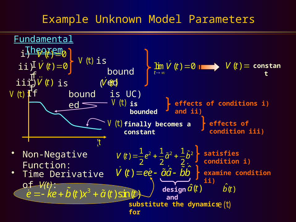
Example Unknown Model Parameters
Fundamental Theorem
V (t) ¸ 0
V (t) ¸ 0
effects of conditions i) and ii)
i) If
ii) IfV (t) ¸ 0is bounded
iii) If is bounded
satisfies condition i)
V (t) ¸ 0
finally becomes a constant
V (t) ¸ 0
• Non-Negative Function:
• Time Derivative of V(t):
is bounded
examine condition ii)
design and
substitute the dynamics for
constant
effects of condition iii)
l imt! 1
e(t) = 0
( ) 0V t ( ) 0V t
( )V t ( )V t
lim ( ) 0t
V t
( )V t
2 2 21 1 1( )
2 2 2V t e a b
ˆ( )a t ˆ( )b t3( ) ( )sin( )e ke b t x a t t
ˆˆ( )V t ee aa bb
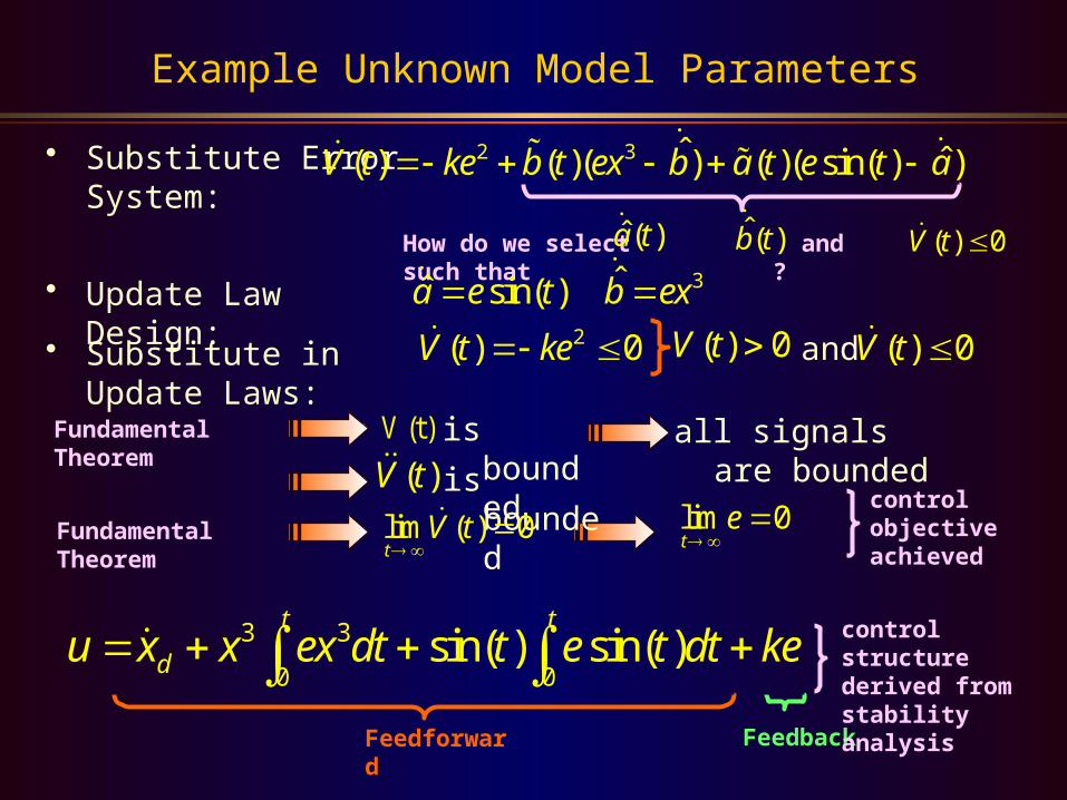
Example Unknown Model Parameters
• Substitute Error System:
How do we select and such that ?
• Update Law Design:
• Substitute in Update Laws:
and
Fundamental Theorem
is boundedV (t) ¸ 0 all signals are bounded
Fundamental Theorem
Feedforward Feedback
control structurederived fromstability analysis
control objective achieved
is bounded
2( ) 0V t ke
ˆ( )b tˆ( )a t
( ) 0V t 3ˆˆ sin( ) a e t b ex
2 3 ˆ ˆ( ) ( )( ) ( )( sin( ) )V t ke b t ex b a t e t a
( )V t
( ) 0V t
lim ( ) 0t
V t
( ) 0V t
lim 0t
e
3 3
0 0sin( ) sin( )
t t
du x x ex dt t e t dt ke
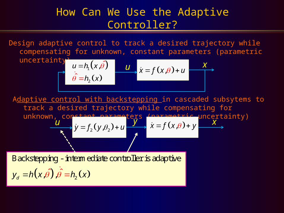
How Can We Use the Adaptive Controller?
Design adaptive control to track a desired trajectory while compensating for unknown, constant parameters (parametric uncertainty)
,x f x u xu
1
2
, ˆ
ˆ
u h x
h x
2
Backstepping - intermediate controller is adaptive
, ˆ ˆ,dy h x h x
Adaptive control with backstepping in cascaded subsytems to track a desired trajectory while compensating for unknown, constant parameters (parametric uncertainty)
,x f x y xy 2 2,y f y u u
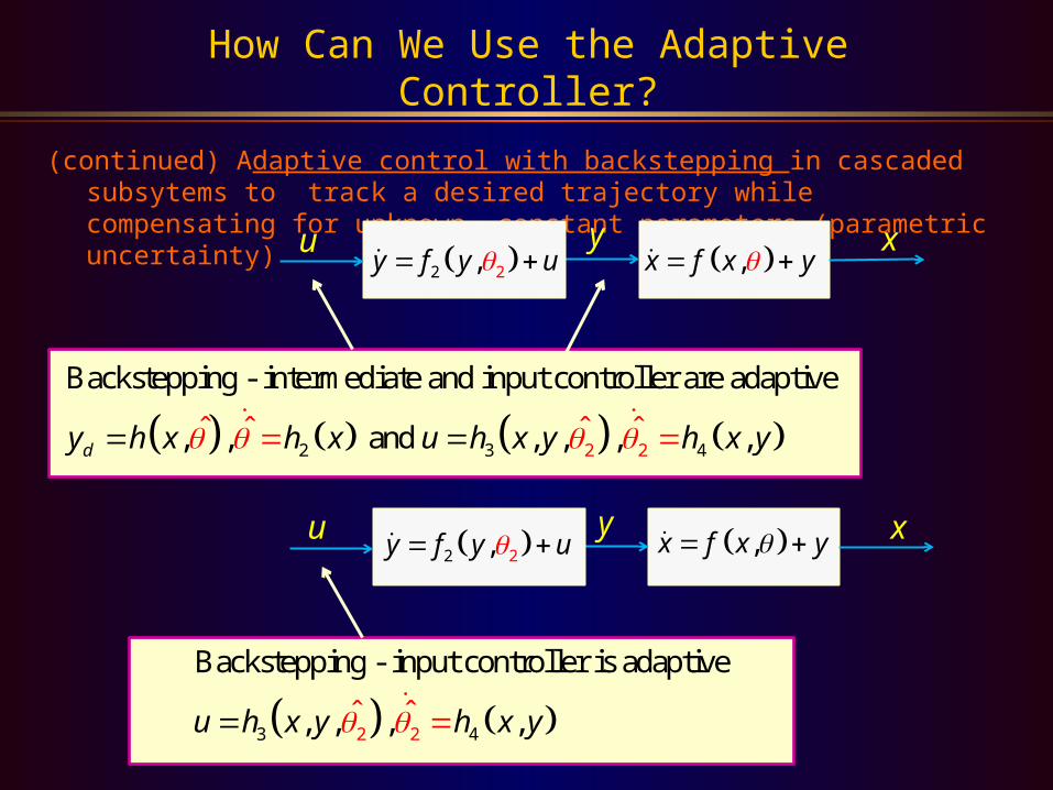
How Can We Use the Adaptive Controller?
2 3 2 42
Backstepping - intermediate and input controller are adaptive
, , and ˆ ˆ ˆ , ˆ, , ,dy h x h x u h x y h x y
(continued) Adaptive control with backstepping in cascaded subsytems to track a desired trajectory while compensating for unknown, constant parameters (parametric uncertainty)
,x f x y xy
22 ,y f y u u
2 23 4
Backstepping - input controller i
ˆ
s adaptive
, , , ˆ ,u h x y h x y
,x f x y xy 22 ,y f y u u
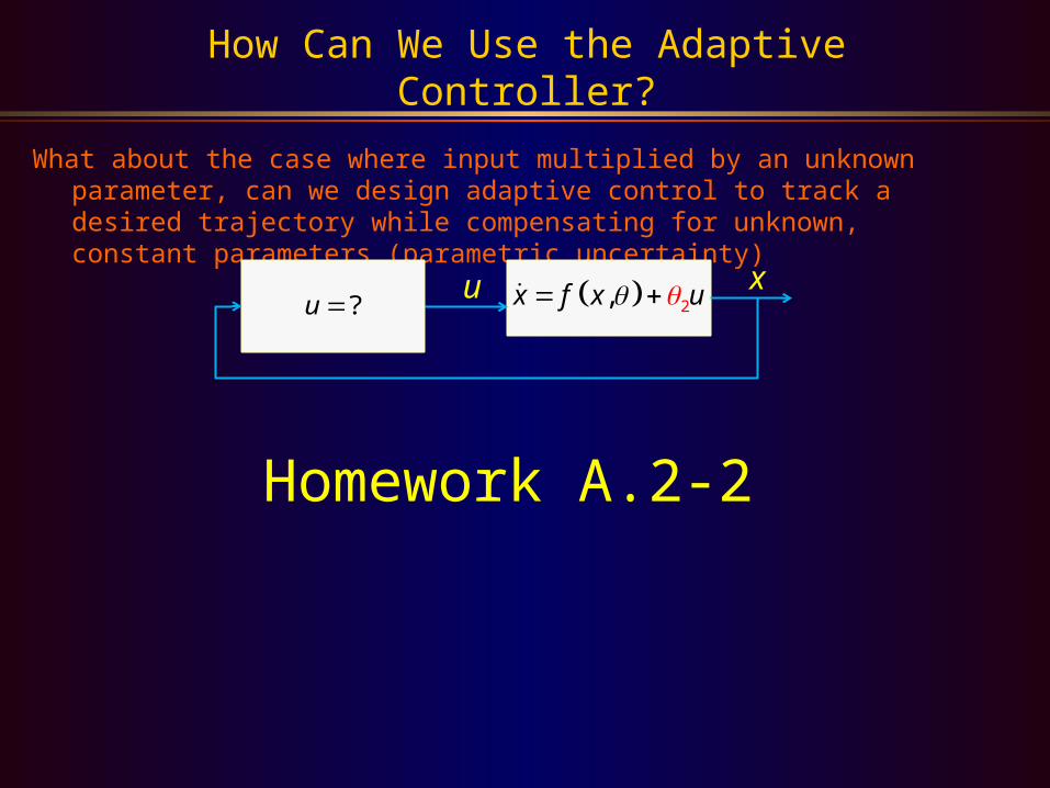
How Can We Use the Adaptive Controller?
What about the case where input multiplied by an unknown parameter, can we design adaptive control to track a desired trajectory while compensating for unknown, constant parameters (parametric uncertainty)
2,x f x u xu?u
Homework A.2-2
24
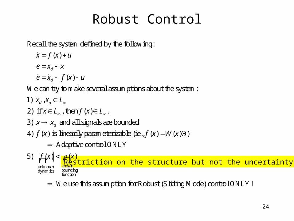
Robust Control
Recall the system defined by the following:
( )
( )
We can try to make several assumptions about the system:
1) ,
2) if , then ( ) .
3) and all si
d
d
d d
d
x f x u
e x x
e x f x u
x x L
x L f x L
x x
knownunknownboundingdynamicsfunction
gnals are bounded
4) ( ) is linearily parameterizable (ie., ( ) ( ) )
Adaptive control ONLY
5) ( ) ( )
We use this assumption for Robust (S
f x f x W x
f x x
liding Mode) control ONLY!
Restriction on the structure but not the uncertainty
25
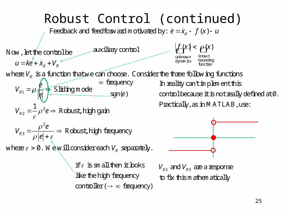
Robust Control (continued)
1
22
2
3
Now, let the control be
where is a function that we can choose. Consider the three following functions
Sliding mode
1 Robust, high gain
Robus
d R
R
R
R
R
u ke x V
V
eV
e
V e
eV
e
t, high frequency
where 0. We will consider each separately.RV
sgn( )e
2 3
In reality can't implement this
control because it is not really defined at 0.
Practically, as in MATLAB, use:
and are a response
to fix this mathematicallyR RV V
auxiliary control
if is small then it looks
like the high frequency
controller ( frequency)
frequency
Feedback and feedforward motivated by: ( )de x f x u
knownunknownboundingdynamicsfunction
( ) ( )f x x
26
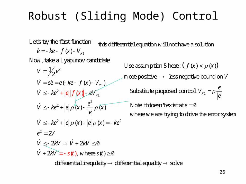
1
2
1
21
22
2 2
Let's try the first function
( )
Now, take a Lyapunov candidate
1 2
( ( ) )
( ) ( )
( ) ( )
( )
R
R
Re
e ke f x V
V e
V ee e ke f x V
V ke eV
eV ke e x x
e
V ke e x e x k
f
e
x
e
2 2
2 2 0
2 , where ( 0( ) )
V
V kV V kV
V kV s t s t
Robust (Sliding Mode) Control
Use assumption 5 here: ( ) ( )
more positive less negative bound on
f x x
V
differential inequlaity differential equality solve
this differential equation will not have a solution
1Substitute proposed control
Note it doesn't exist at 0
where we are trying to drive the error system
R
eV
e
e

27
Robust (Sliding Mode) Control (continued)
0
2 2
Solving the differential equation, we get
( ) (0)exp( 2 ) exp( 2 ) exp(2 ) ( )
( ) (0)exp( 2 )
1 1 ( ) (0)exp( 2 )2 2 ( ) (0) exp( )
So, the system is globally exponent
t
V t V kt kt k s d
V t V kt
e t e kt
e t e kt
ially stable, and all signals are bounded!
always negative
upper bound
Base of the natural
logarithm.
28
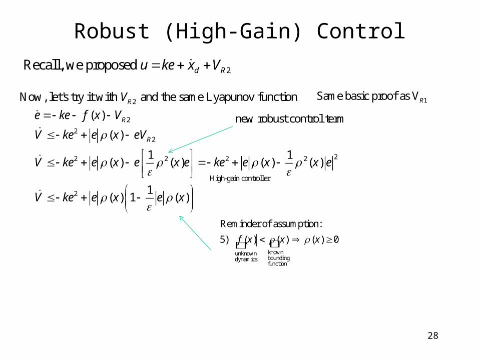
2
2
22
22 2 2 2
2
Now, let's try it with and the same Lyapunov function
( )
( )
1 1 ( ) ( ) ( ) ( )
1 ( ) 1 ( )
R
R
R
V
e ke f x V
V ke e x eV
V ke e x e x e ke e x x e
V ke e x e x
Robust (High-Gain) Control
new robust control term
1Same basic proof as VR
knownunknownboundingdynamicsfunction
Reminder of assumption:
5) ( ) ( ) ( ) 0f x x x
2Recall, we proposed d Ru ke x V
High-gain controller
29
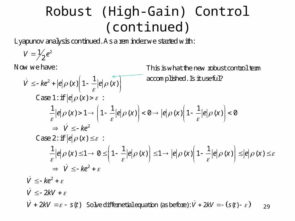
2
2
Lyapunov analysis continued. As a reminder we started with:
1 2Now we have:
1 ( ) 1 ( )
V e
V ke e x e x
Robust (High-Gain) Control (continued)
This is what the new robust control term
accomplished. Is it useful?
Solve differnetial equation (as before): 2 ( )V kV s t
2
Case 1: if ( ) :
1 1 1 ( ) 1 1 ( ) 0 ( ) 1 ( ) 0
Case 2: if ( ) :
1 1 ( ) 1 0 1 ( ) 1
e x
e x e x e x e x
V kee x
e x e x
2
2
1( ) 1 ( ) ( )
2
2 ( )
e x e x e x
V ke
V ke
V kV
V kV s t
30
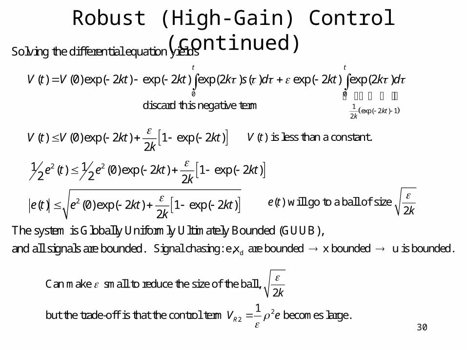
Robust (High-Gain) Control (continued)
0 0
1exp( 2 ) 1
2
2 2
Solving the differential equation yields
( ) (0)exp( 2 ) exp( 2 ) exp(2 ) ( ) exp( 2 ) exp(2 )
( ) (0)exp( 2 ) 1 exp( 2 )2
1 1 ( ) (0)exp( 22 2
t t
ktk
V t V kt kt k s d kt k d
V t V kt ktk
e t e k
2
) 1 exp( 2 )2
( ) (0)exp( 2 ) 1 exp( 2 )2
The system is Globally Uniformly Ultimately Bounded (GUUB),
and all signals are bounded.
t ktk
e t e kt ktk
discard this negative term
( ) is less than a constant.V t
( ) will go to a ball of size 2
e tk
22
Can make small to reduce the size of the ball, 2
1but the trade-off is that the control term becomes large.R
k
V e
dSignal chasing: e,x are bounded x bounded u is bounded.
31
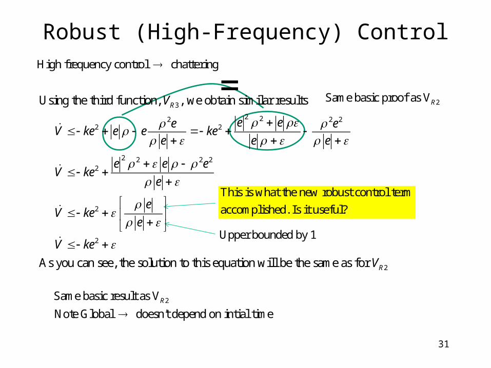
3
2 22 2 22 2
2 2 2 22
2
2
Using the third function, , we obtain similar results
As you can see, the sol
RV
e ee eV ke e e ke
e e e
e e eV ke
e
eV ke
e
V ke
2ution to this equation will be the same as for RV
Robust (High-Frequency) ControlHigh frequency control chattering
2Same basic proof as VR
2Same basic result as V
Note Global doesn't depend on intial timeR
Upper bounded by 1
This is what the new robust control term
accomplished. Is it useful?
=
32
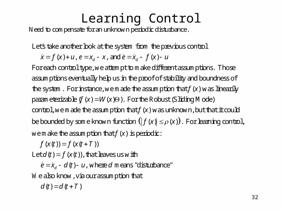
Let's take another look at the system from the previous control
( ) , , and ( )
For each control type, we attempt to make different assumptions. Those
assumptions eventually he
d dx f x u e x x e x f x u
lp us in the proof of stability and boundness of
the system. For instance, we made the assumption that ( ) was linearily
parameterizable ( ( ) ( ) ). For the Robust (Sliding Mode)
control, we made th
f x
f x W x
e assumption that ( ) was unknown, but that it could
be bounded by some known function ( ) ( ) . For learning control,
we make the assumption that ( ) is periodic:
( ( )) ( ( ))
Let ( ) ( (
f x
f x x
f x
f x t f x t T
d t f x
)), that leaves us with
( ) , where means "disturbance"
We also know, via our assumption that
( ) ( )
d
t
e x d t u d
d t d t T
Learning ControlNeed to compensate for an unknown periodic disturbance.
33
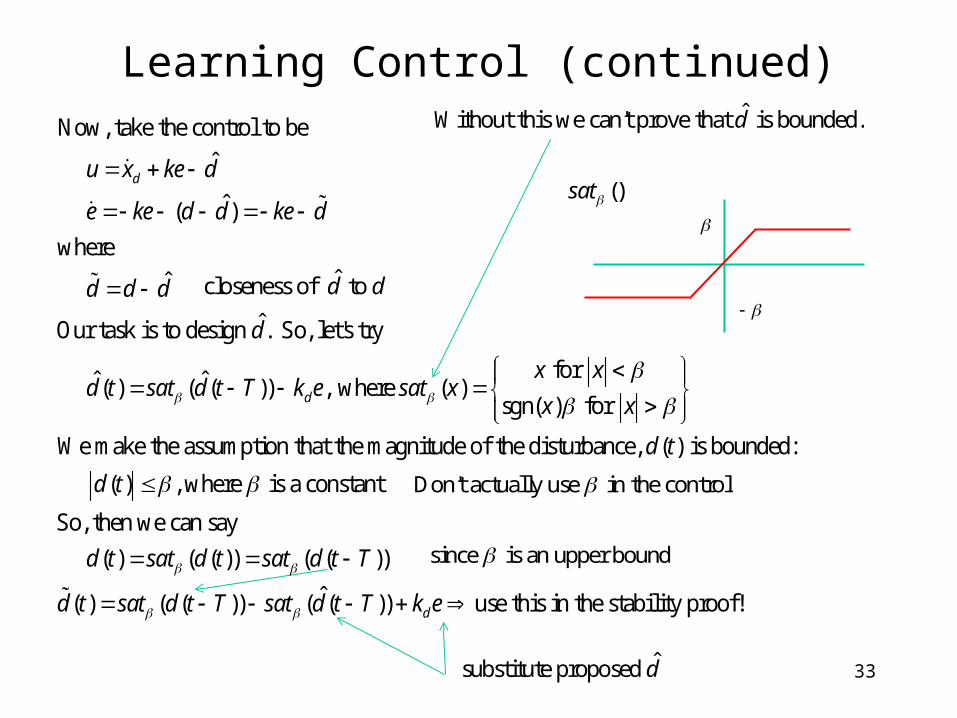
Learning Control (continued)
Now, take the control to be
ˆ
ˆ ( )
where
ˆ
ˆOur task is to design . So, let's try
for ˆ ˆ ( ) ( ( )) , where ( )sgn( ) for
d
d
u x ke d
e ke d d ke d
d d d
d
x xd t sat d t T k e sat x
x x
We make the assumption that the magnitude of the disturbance, ( ) is bounded:
( ) , where is a constant
So, then we can say
( ) ( ( )) ( ( ))
ˆ( ) ( ( )) ( ( ))
d t
d t
d t sat d t sat d t T
d t sat d t T sat d t T
use this in the stability proof!dk e
ˆWithout this we can't prove that is bounded.d
() sat
Don't actually use in the control
since is an upper bound
ˆsubstitute proposed d
ˆcloseness of to d d
34
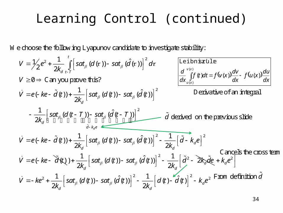
Learning Control (continued)
22
2
We choose the following Lyapunov candidate to investigate stability:
1 ˆ1 ( ( )) ( ( ))2 2
0 Can you prove this?
1 ˆ ( ( )) ( ( )) ( ( ))2
t
d t T
d
V e sat d sat d dk
V
V e ke d t sat d t sat d tk
2
2 2
1 ˆ ( ( )) ( ( ))2
1 1ˆ ( ( )) ( ( )) ( ( ))2 2
( ( )
d
dd k e
dd d
sat d t T sat d t Tk
V e ke d t sat d t sat d t d k ek k
V e ke d t
221 1ˆ) ( ( )) ( ( )) 2
2 2 dd d
sat d t sat d t d k dek k
2
2 22 21 1ˆ ˆ ( ( )) ( ( )) ( ) ( )
2 2
d
dd d
k e
V ke sat d t sat d t d t d t k ek k
dx
duxuf
dx
dvxvfdttf
dx
dxv
xu
)()()(
:rule sLeibniz')(
)(
Derivative of an integral
derived on the previous slided
Cancels the cross term
From definition d
35
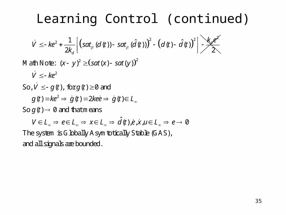
Learning Control (continued)
22 2
2 1 ˆ ˆ ( ( )) ( ( )) ( ) ( )2 2
d
d
k eV ke sat d t sat d t d t d t
k
22
2
2
Math Note: ( ) ( ) ( )
So, ( ), for ( ) 0 and
( ) ( ) 2 ( )
So ( ) 0 and that means
ˆ ( ), , , 0
The system is Globally Asymto
x y sat x sat y
V ke
V g t g t
g t ke g t kee g t L
g t
V L e L x L d t e x u L e
tically Stable (GAS),
and all signals are bounded.
36
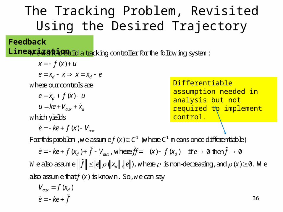
The Tracking Problem, RevisitedUsing the Desired Trajectory
We want to build a tracking controller for the following system:
( )
where our controls are
( )
which yields
( )
For this pro
d d
d
aux d
aux
x f x u
e x x x x e
e x f x u
u ke V x
e ke f x V
1 1blem, we assume ( ) (where C means once differentiable)
( ) , where ( ) ( )
We also assume ( , ), where is non-decreasing, and ( ) 0. We
also assume that ( ) is
d aux d
d
f x C
e ke f x f V f f x f x
f e x e x
f x
known. So, we can say
( )
aux dV f x
e ke f
Differentiable assumption needed in analysis but not required to implement control.
if 0 then 0e f
Feedback Linearization
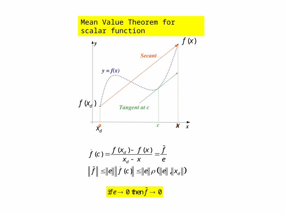
( )f x
xdx
( )df x
( ) ( )( )
( ) ,
d
d
d
f x f x ff c
x x e
f e f c e e x
Mean Value Theorem for scalar function
if 0 then 0e f
38
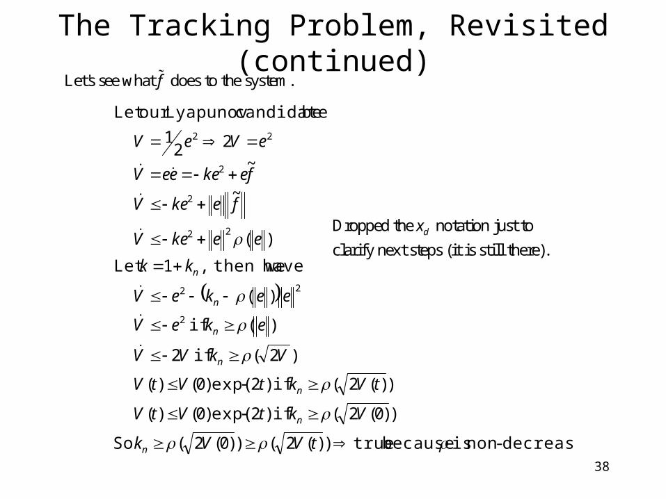
The Tracking Problem, Revisited (continued)
decreasing-non is because true))(2())0(2( So
))0(2( if )2exp()0()(
))(2( if )2exp()0()(
)2( if 2
)( if
)(
have then we,1Let
)(
~
~
221
be candidate Lyapunovour Let
2
22
22
2
2
22
tVVk
VktVtV
tVktVtV
VkVV
ekeV
eekeV
kk
eekeV
fekeV
fekeeeV
eVeV
n
n
n
n
n
n
n
Let's see what does to the system.f
Dropped the notation just to
clarify next steps (it is still there).dx
39
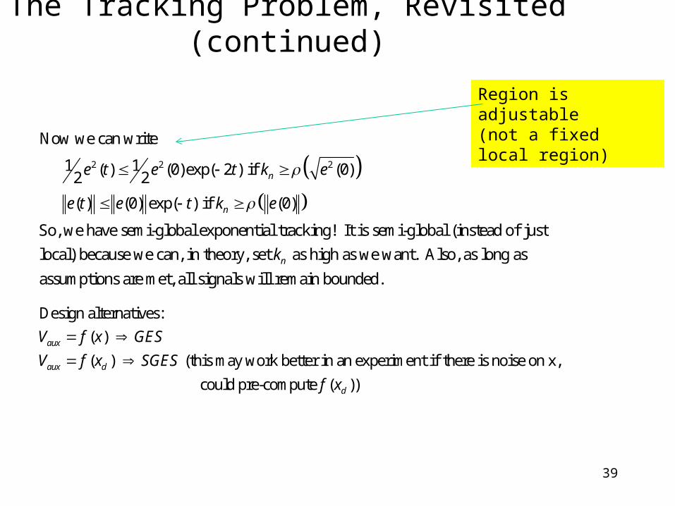
2 2 2
Now we can write
1 1 ( ) (0)exp( 2 ) if (0)2 2
( ) (0) exp( ) if (0)
So, we have semi-global exponential tracking! It is semi-global (instead of just
local) because we can, in the
n
n
e t e t k e
e t e t k e
ory, set as high as we want. Also, as long as
assumptions are met, all signals will remain bounded.nk
The Tracking Problem, Revisited (continued)
Region is adjustable(not a fixed local region)
Design alternatives:
( )
( ) (this may work better in an experiment if there is noise on x,
could pre-compute ( ))
aux
aux d
d
V f x GES
V f x SGES
f x
40
Adaptive Control
40
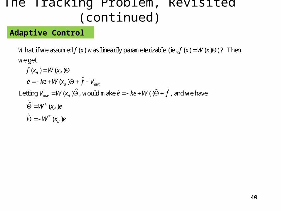
What if we assumed ( ) was linearily parameterizable (ie., ( ) ( ) )? Then
we get
( ) ( )
( )
ˆLetting ( ) , would make ( ) , and we have
ˆ
d d
d aux
aux d
T
f x f x W x
f x W x
e ke W x f V
V W x e ke W f
W
( )
( )
d
Td
x e
W x e
The Tracking Problem, Revisited (continued)
41
The Tracking Problem, Revisited (continued)
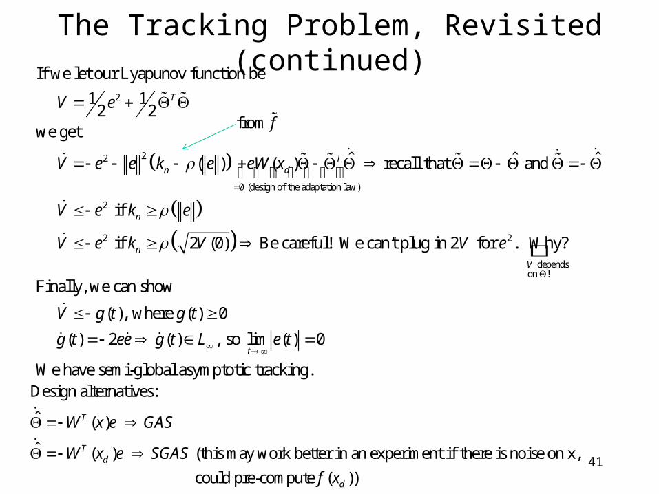
2
22
0 (design of the adaptation law)
2
If we let our Lyapunov function be
1 1 2 2we get
ˆ ˆ ˆ ( ) ( ) recall that and
if
T
Tn d
n
V e
V e e k e eW x
V e k e
V
2 2
dependson !
if 2 (0) Be careful! We can't plug in 2 for . Why?
Finally, we can show
( ), where ( ) 0
( ) 2 ( ) , so lim ( ) 0
We have semi-global asymptotic trac
n
V
t
e k V V e
V g t g t
g t ee g t L e t
king.
from f
Design alternatives:
ˆ ( )
ˆ ( ) (this may work better in an experiment if there is noise on x,
could pre-compute ( ))
T
Td
d
W x e GAS
W x e SGAS
f x
42
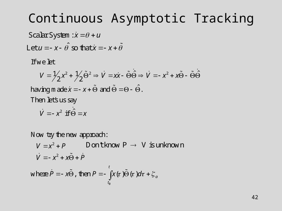
Continuous Asymptotic Tracking
2 2 2
2
2
2
If we let
ˆ ˆ1 1 2 2ˆhaving made and .
Then let's us say
ˆ if
Now try the new approach:
where , then
V x V xx V x x
x x
V x x
V x P
V x x P
P x P x
0
( ) ( )t
a
t
d
Scalar System:
ˆLet so that
x u
u x x x
Don't know P V is unknown
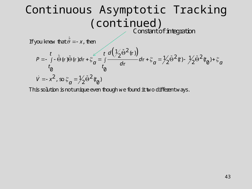
43
If you knew that , then
21 ( )2 2 21 1 ( ) ( ) ( ) ( )2 2 00 02 21 , so ( )2 0
This solution is not unique even though we found it two different ways.
x
dt tP d d t t
a a adt t
V x ta
Continuous Asymptotic Tracking (continued)Constant of integration
44
Continuous Asymptotic Tracking (continued)
Lx
xf
x
xfxfL
x
xm
x
xmxm
Lx
Lx
xf
x
xfxfL
x
xm
x
xmxm
Cx
xm
xfxgxfxgxmuxfxxm
txtx
xg
gfuxgxfx
d
d
d
dd
d
d
d
dd
d
d
2
2
2
2
2
2
2
2
3
11
)(,
)(),( and
)(,
)(),( A3)
as long as
)(,
)(),( and
)(,
)(),( A2)
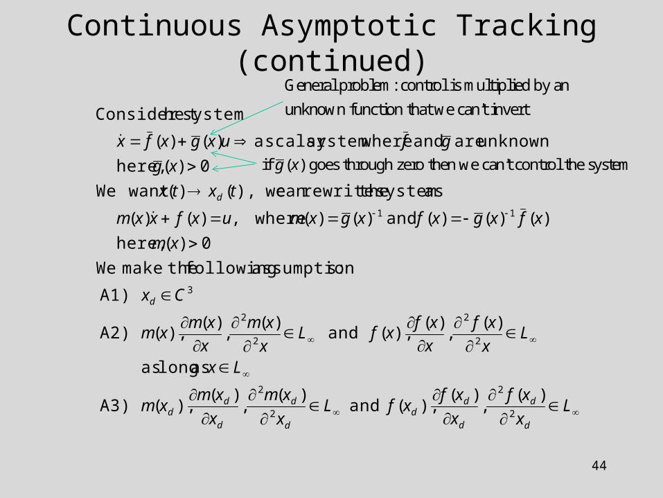
A1)
:sassumption following themake We
0)( here,
)()()( and )()( where,)()(
as system therewritecan we),()( want We
0)( here,
unknown are and wheresystemscalar a)()(
system heConsider t
if ( ) goes through zero then we can't control the systemg x
General problem: control is multiplied by an
unknown function that we can't invert
45
Continuous Asymptotic Tracking (continued)
true?). thisis(Why then , if and ,0 then ,0 if shown that becan It
as variablenew a define sLet'
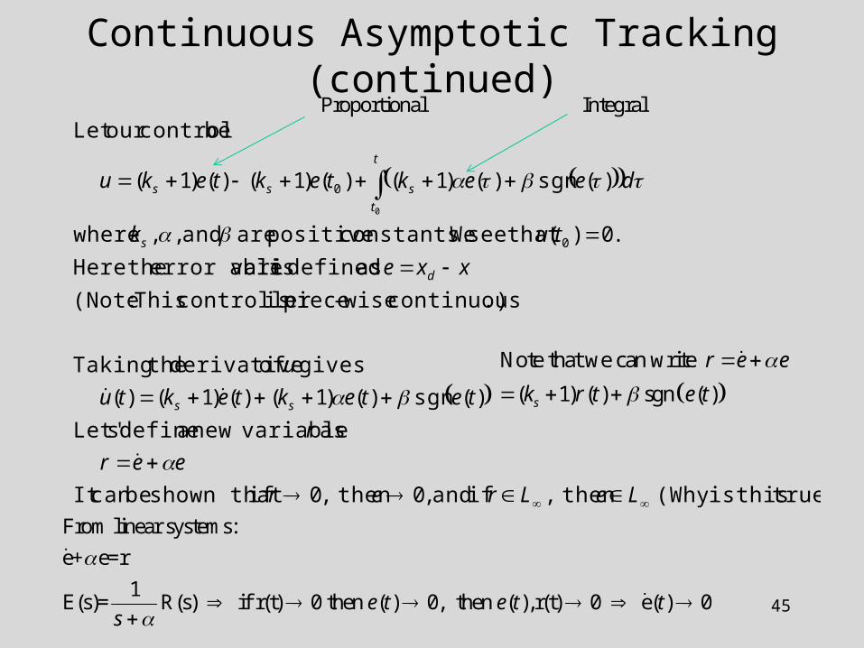
)(sgn)()1()()1()(
gives of derivative theTaking
.)continuous wise-piece is controller This :(Note
as defined is ableerror vari theHere
.0)( that see Weconstants. positive are and , , where
)(sgn)()1()()1()()1(
be controlour Let
0
0
0
LeLrer
eer
r
tetektektu
u
xxe
tuk
deektekteku
ss
d
s
t
t
sss
Proportional Integral
From linear systems:
e+ e=r
1E(s)= R(s) if r(t) 0 then ( ) 0, then ( ), r(t) 0 e( ) 0 e t e t t
s
Note that we can write
( 1) ( ) sgn ( )s
r e e
k r t e t
46
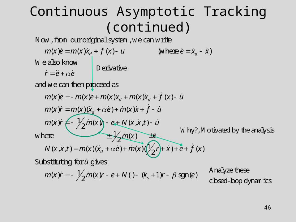
Now, from our original system, we can write
( ) ( ) ( ) (where )
We also know
and we can then proceed as
( ) ( ) ( ) ( ) (
d d
d d
m x e m x x f x u e x x
r e e
m x e m x e m x x m x x f
)
( ) ( )( ) ( )
1 ( ) ( ) ( , , )2where
1 ( , , ) ( )( ) ( )( ) ( )2Substituting for gives
1 ( ) ( ) ( ) ( 1)2
d
d
s
x u
m x r m x x e m x x f u
m x r m x r e N x x t u
N x x t m x x e m x r x e f x
u
m x r m x r e N k r
sgn( )e
Continuous Asymptotic Tracking (continued)
Derivative
1 ( )2 m x eWhy?, Motivated by the analysis
Analyze these
closed-loop dynamics
47
2 2
2
2 2
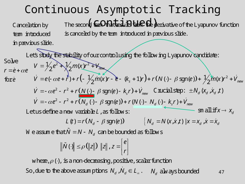
Let's study the stability of our control using the following Lyapunov candidate:
1 1 ( )2 21 1 ( ) ( ) ( 1) ( ) sgn( ) ( )2 2
( ) sgn(
new
s new
V e m x r V
V e e r r m x r e k r r N e m x r V
V e r r N e
2 2
)
( ) sgn( ) ( ( ) ( ) )
Let us define a new variable , as follows:
( ) sgn( ) ( , , ) | ,
We assume that
s new
d d s new
d d d d
k r V
V e r r N e r N N k r V
L
L t r N e N N x x t x x x x
can be bounded as follows
( ) ,
where, ( ), is a non-decreasing, positive, scalar function
So, due to the above assumptions , .
d
d d
N N N
eN z z z
r
N N L
Continuous Asymptotic Tracking (continued)The second term that results from the derivative of the Lyapunov function
is canceled by the term introduced in previous slide.
Solve
for
r e e
e
Cancelation by
term introduced
in previous slide.
Crucial step: ( , , )d d dN x x t
always boundeddN
small if dx x
48
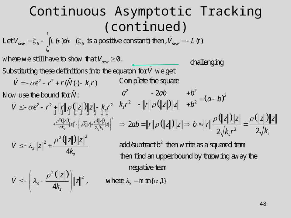
0
2 2
Let ( ) ( is a positive constant) then, ( )
where we still have to show that 0.
Substituting these definitions into the equaton for we get
( ( )
t
new b b new
t
new
s
V L d V L t
V
V
V e r r N k r
222
2 2 2
4 2
222
3
22
3 3
)
Now use the bound for :
4
, where min{ ,1}4
ss s
s
z zz k r z
k k
s
s
N
V e r r z z k r
z zV z
k
zV z
k
Continuous Asymptotic Tracking (continued)
challenging
2 22
2 2
2
2
Complete the square
2
222
add/subtract b then write as a squared term
then find an upper bound by throwing away the
negative term
s
ss
a ab ba b
k r r z z b
z z z zab r z z b r
kk r
49
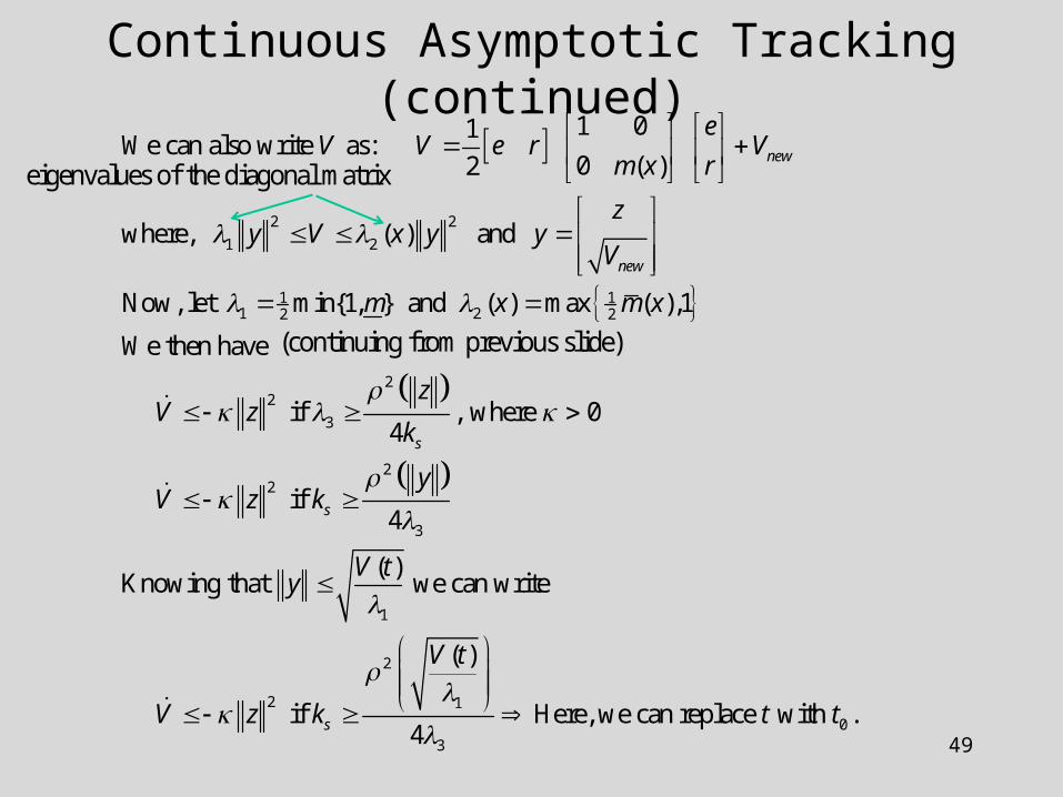
2 2
1 2
1 11 22 2
22
3
1 01We can also write as:
0 ( )2
where, ( ) and
Now, let min{1, } and ( ) max ( ),1
We then have
if , where4
new
new
s
eV V e r V
m x r
zy V x y y
V
m x m x
zV z
k
22
3
1
2
2 1
03
0
if 4
( )Knowing that we can write
( )
if Here, we can replace with .4
s
s
yV z k
V ty
V t
V z k t t
Continuous Asymptotic Tracking (continued)
eigenvalues of the diagonal matrix
(continuing from previous slide)
50
Continuous Asymptotic Tracking (continued)
2 2
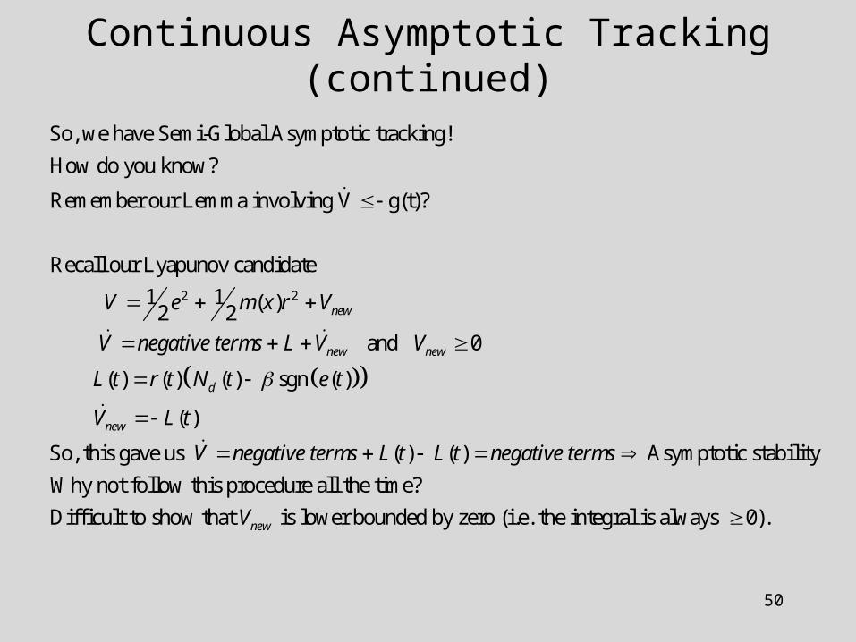
So, we have Semi-Global Asymptotic tracking!
How do you know?
Remember our Lemma involving V g(t)?
Recall our Lyapunov candidate
1 1 ( )2 2
and
new
new
V e m x r V
V negative terms L V
0
( ) ( ) ( ) sgn ( )
( )
So, this gave us ( ) ( ) Asymptotic stability
Why not follow this procedure all the time?
Difficult to show t
new
d
new
V
L t r t N t e t
V L t
V negative terms L t L t negative terms
hat is lower bounded by zero (i.e. the integral is always 0).newV
51
Continuous Asymptotic Tracking (continued)
0
0 0
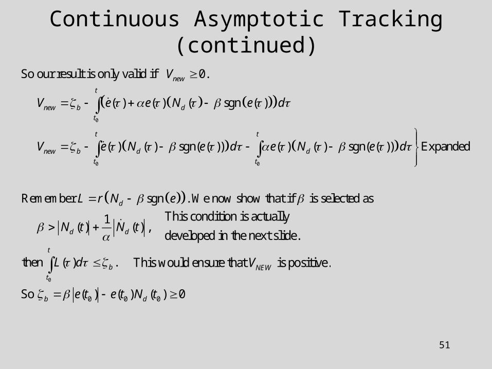
So our result is only valid if 0.
( ) ( ) ( sgn ( )
( ) ( ) sgn( ( )) ( ) ( ) sgn( ( )) Expanded
Remember sgn . We now show th
new
t
new b d
t
t t
new b d d
t t
d
V
V e e N e d
V e N e d e N e d
L r N e
0
0 0 0
at if is selected as
1 ( ) ( ) ,
then ( ) .
So ( ) ( ) ( ) 0
d d
t
b
t
b d
N t N t
L d
e t e t N t
This condition is actually
developed in the next slide.
This would ensure that is positive.NEWV
52
Continuous Asymptotic Tracking (continued)
0 0 0 0
0 0
0 0
Integrate by parts
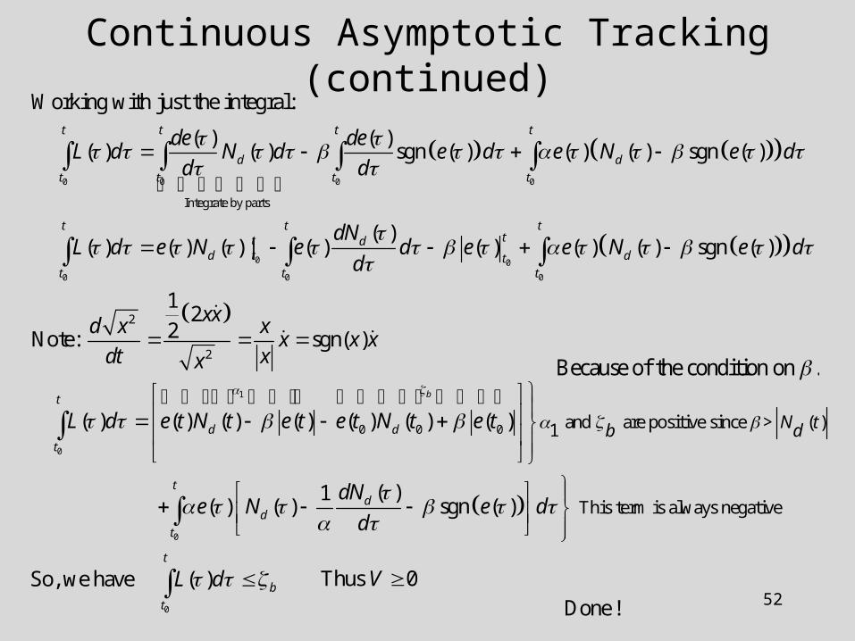
Working with just the integral:
( ) ( ) ( ) ( ) sgn ( ) ( ) ( ) sgn ( )
( ) ( ) ( ) ( ) | ( ) ( ) (
t t t t
d d
t t t t
t ttt d
d t tt t
de deL d N d e d e N e d
d d
dNL d e N e d e e
d
0
1
0
2
2
0 0 0 and are positive since > ( )1
) ( ) sgn ( )
12
2Note: sgn( )
( ) ( ) ( ) ( ) ( ) ( ) ( )
b
t
d
t
t
d d
t
N tb d
N e d
xxd x x
x x xdt xx
L d e t N t e t e t N t e t
0
0
This term is always negative( )1
( ) ( ) sgn ( )
So, we have ( )
td
d
t
t
b
t
dNe N e d
d
L d
Because of the condition on .
Thus 0V Done !

53
Feedback Linearization for Second-Order Systems
dmmpv
mpvd
pv
mpvd
md
m
d
mT
m
qMMNNqVVekekMeM
NqVekekqM
ekeke
NqVekekqM
NqVqMeM
qFqGqqNqqNqqqVqqM
qqe
xqqVqMx
qMqFqGqqqVqqM
)ˆ(ˆ)ˆ()(ˆ
ˆˆ)(ˆ
try weifWhat
0
)(
can write wemodel), (the system about the everything know weIf
))()(),(( ),(),()(
as system therewrite could We
0),()(21
symmetric. definite, positive is )( where,)()(),()(
system heConsider t
General Dynamic Equation for an n-link Robot
54
Feedback Linearization Problem (continued)
1 1
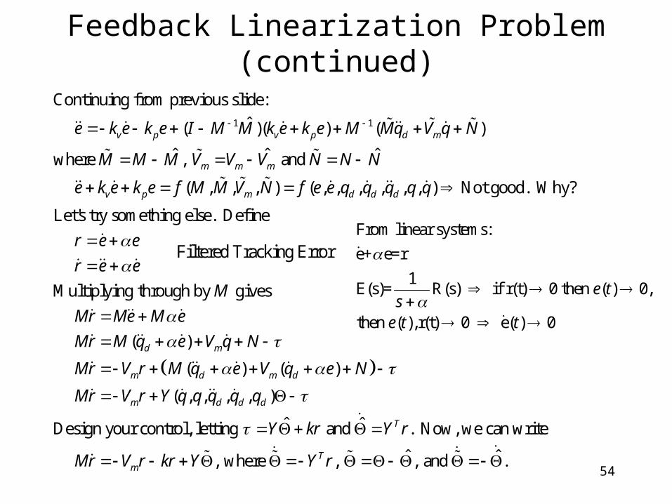
Continuing from previous slide:
ˆ ( )( ) ( )
ˆ ˆ ˆwhere , and
( , , , ) ( , , , , , , ) Not good. Why?
v p v p d m
m m m
v p m d d d
e k e k e I M M k e k e M Mq V q N
M M M V V V N N N
e k e k e f M M V N f e e q q q q q
Let's try something else. Define
Multiplying through by gives
( )
( ) ( )
( , ,
d m
m d m d
m
r e e
r e e
M
Mr Me M e
Mr M q e V q N
Mr V r M q e V q e N
Mr V r Y q q
, , )
ˆ ˆDesign your control, letting and . Now, we can write
ˆ ˆ , where , , and .
d d d
T
Tm
q q q
Y kr Y r
Mr V r kr Y Y r
Filtered Tracking ErrorFrom linear systems:
e+ e=r
1E(s)= R(s) if r(t) 0 then ( ) 0,
then ( ), r(t) 0 e( ) 0
e ts
e t t
55
Feedback Linearization Problem (continued)
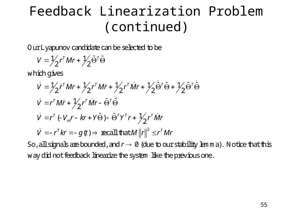
Our Lyapunov candidate can be selected to be
1 1 2 2which gives
1 1 1 1 1 2 2 2 2 2
ˆ1 21 ( ) 2
T T
T T T T T
T T T
T T T Tm
V r Mr
V r Mr r Mr r Mr
V r Mr r Mr
V r V r kr Y Y r r Mr
V
2( ) recall that
So, all signals are bounded, and 0 (due to our stability lemma). Notice that this
way did not feedback linearize the system like the previous one.
T Tr kr g t M r r Mr
r
56
Feedback Linearization Problem (continued)
212
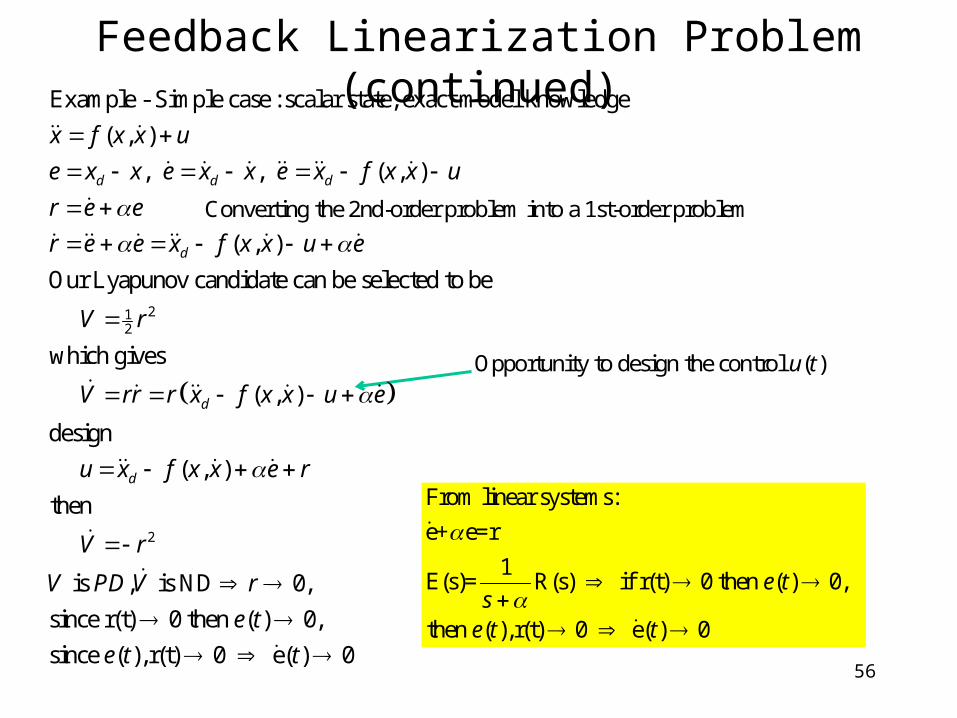
Example - Simple case : scalar state, exact model knowledge
( , )
, , ( , )
( , )
Our Lyapunov candidate can be selected to be
d d d
d
x f x x u
e x x e x x e x f x x u
r e e
r e e x f x x u e
V r
2
which gives
( , )
design
( , )
then
is , is ND 0,
since r(t) 0 then ( ) 0,
since ( ), r(t) 0 e( ) 0
d
d
V rr r x f x x u e
u x f x x e r
V r
V PD V r
e t
e t t
From linear systems:
e+ e=r
1E(s)= R(s) if r(t) 0 then ( ) 0,
then ( ), r(t) 0 e( ) 0
e ts
e t t
Converting the 2nd-order problem into a 1st-order problem
Opportunity to design the control ( )u t
57
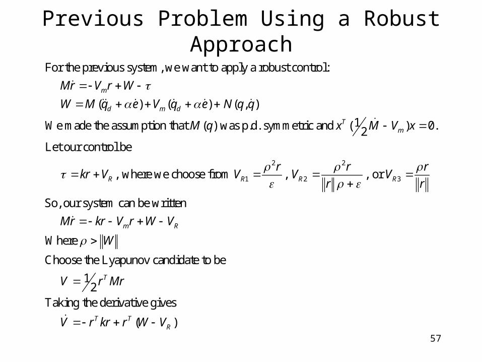
For the previous system, we want to apply a robust control:
( ) ( ) ( , )
1We made the assumption that ( ) was p.d. symmetric and ( ) 0.2Let our control
m
d m d
Tm
Mr V r W
W M q e V q e N q q
M q x M V x
2 2
1 2 3
be
, where we choose from , , or
So, our system can be written
Where
Choose the Lyapunov candidate to be
1 2Taking the derivative
R R R R
m R
T
r r rkr V V V V
r r
Mr kr V r W V
W
V r Mr
gives
( )T TRV r kr r W V
Previous Problem Using a Robust Approach
58
Previous Problem Using a Robust Approach
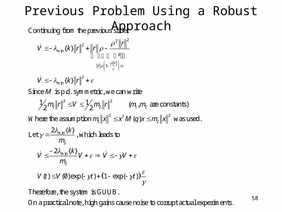
222
min
1
2
min
2 2
1 2 1 2
Continuing from the previous slide:
{ }
{ }
Since is p.d. symmetric, we can write
1 1 ( , are constants)2 2
Where
rr
rV k r r
V k r
M
m r V m r m m
2 2
1 2
min
2
min
2
the assumption ( ) was used.
2 { }Let , which leads to
2 { }
( ) (0)exp( ) 1 exp( )
Therefore, the system is GUUB.
On a practical note, high ga
Tm x x M q x m x
k
m
kV V V V
m
V t V t t
ins cause noise to corrupt actual experiments.
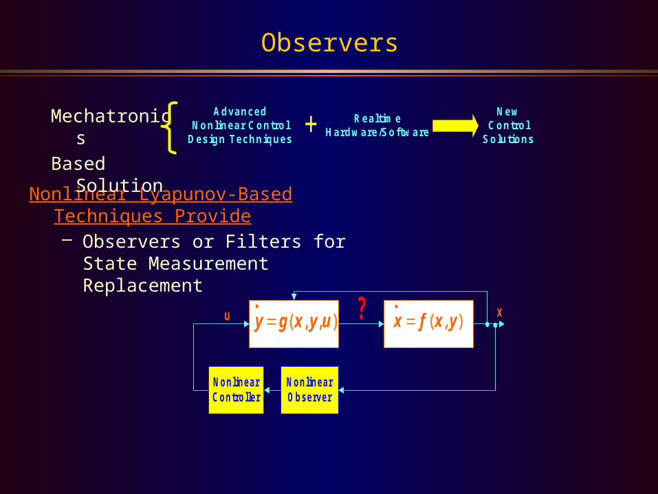
Nonlinear Lyapunov-Based Techniques Provide– Observers or Filters for State
Measurement Replacement
Observers
Mechatronics
Based Solution
AdvancedNonlinear Control
Design Techniques
RealtimeHardw are/Softw are+
NewControl
Solutions
x f x y·
( , )y g x y u·
( , , )u ? x
NonlinearObserver
NonlinearController

Estimate of the State
Observers Alone
x f x y· ( , )y g x yu
·
= ( , , )u ? x
Nonlinear
Observer
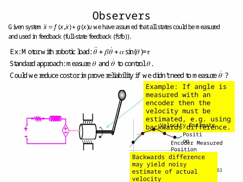
Ex: Motor with robotic load: sin( )=
Standard approach: measure and to control .
Could we reduce cost or improve reliability if we didn't need to measure ?
61
ObserversGiven system ( , ) ( ) we have assumed that all states could be measured
and used in feedback (full-state feedback (fsfb)).
x f x x g x u
Example: If angle is measured with an encoder then the velocity must be estimated, e.g. using backwards difference.
Encoder Measured Position
Position
Velocity Estimate
Backwards difference may yield noisy estimate of actual velocity
62
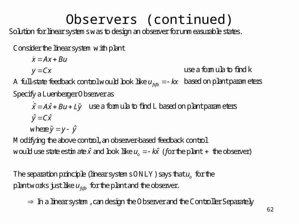
Observers (continued)
Consider the linear system with plant
A full-state feedback control would look like
Specify a Luenberger Observer as
ˆ ˆ
ˆ ˆ
fsfb
x Ax Bu
y Cx
u kx
x Ax Bu Ly
y Cx
ˆ where
Modifying the above control, an observer-based feedback control
ˆ ˆwould use state estimate and look like ( or the plant the observer)
The separation principle (linear sys
o
y y y
x u kx f
tems ONLY) says that for the
plant works just like for the plant and the observer.o
fsfb
u
u
Solution for linear systems was to design an observer for unmeasurable states.
In a linear system, can design the Observer and the Controller Separately
use a formula to find L based on plant parameters
use a formula to find k
based on plant parameters
63
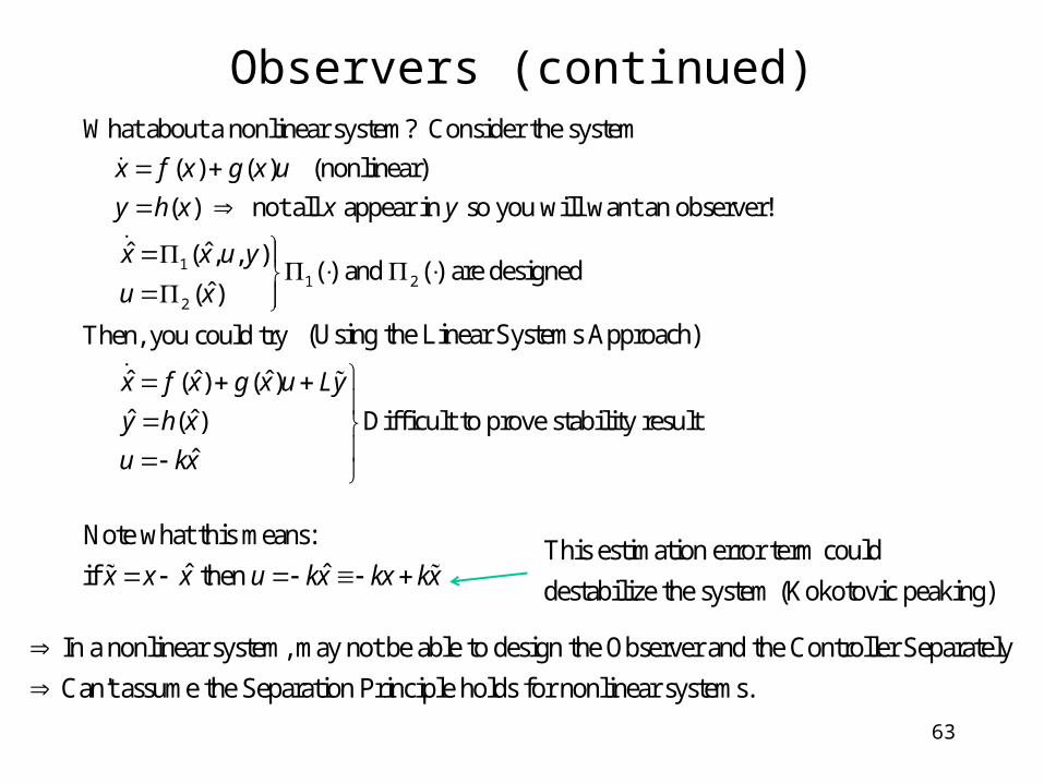
Observers (continued)
11 2
2
What about a nonlinear system? Consider the system
( ) ( ) (nonlinear)
( ) not all appear in so you will want an observer!
ˆ ˆ( , , ) ( ) and ( ) are
ˆ( )
x f x g x u
y h x x y
x x u y
u x
designed
Then, you could try
ˆ ˆ ˆ( ) ( )
ˆ ˆ ( ) Difficult to prove stability result
ˆ
x f x g x u Ly
y h x
u kx
(Using the Linear Systems Approach)
Note what this means:
ˆ ˆif then x x x u kx kx kx This estimation error term could
destabilize the system (Kokotovic peaking)
In a nonlinear system, may not be able to design the Observer and the Controller Separately
Can't assume the Separation Principle holds for nonlinear systems.
64
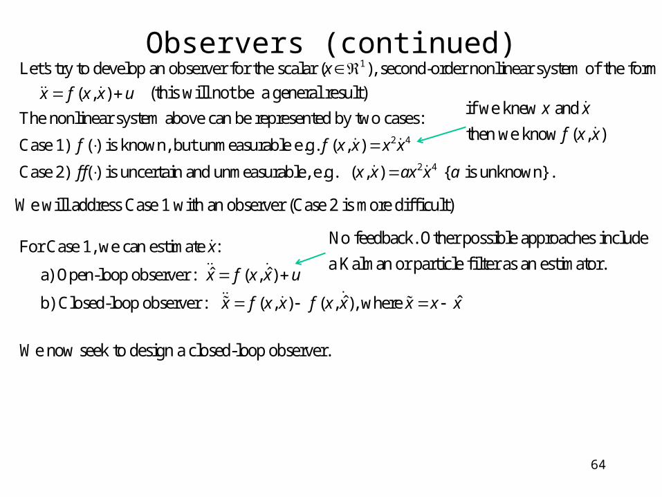
Observers (continued)1Let's try to develop an observer for the scalar ( ), second-order nonlinear system of the form
( , )
The nonlinear system above can be represented by two cases:
Case 1) ( ) is known, bu
x
x f x x u
f
2 4
2 4
t unmeasurable e.g. ( , )
Case 2) ( ) is uncertain and unmeasurable, e.g. ( , ) { is unknown}.
For Case 1, we can estimate :
ˆ ˆ a) Open-loop observer : ( , )
b) Cl
f x x x x
f f x x ax x a
x
x f x x u
ˆ ˆosed-loop observer : ( , ) ( , ), where x f x x f x x x x x
No feedback. Other possible approaches include
a Kalman or particle filter as an estimator.
if we knew and
then we know ( , )
x x
f x x
We will address Case 1 with an observer (Case 2 is more difficult)
(this will not be a general result)
We now seek to design a closed-loop observer.
65
Observers (continued)
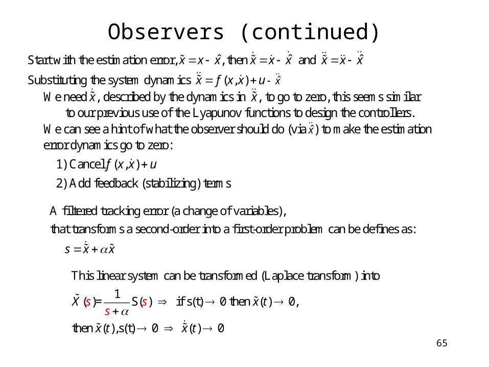
A filtered tracking error (a change of variables),
that transforms a second-order into a first-order problem can be defines as:
s x x
ˆ
ˆ ˆ ˆStart with the estimation error, , then and
Substituting the system dynamics ( , ) x
x x x x x x x x x
x f x x u
We need , described by the dynamics in , to go to zero, this seems similar to our previous use of the Lyapunov functions to design the controllers. We can see a hint of what the obse
x x
ˆrver should do (via ) to make the estimationerror dynamics go to zero:
1) Cancel ( , )
2) Add feedback (stabilizing) terms
x
f x x u
This linear system can be transformed (Laplace transform) into
1( )= S( ) if s(t) 0 then ( ) 0,
then ( ),s(t) 0 ( ) 0
X x t
x t x
s
t
ss
66
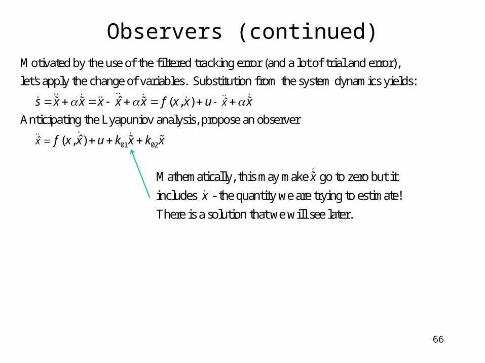
Observers (continued)
Mathematically, this may make go to zero but it
includes - the quantity we are trying to estimate!
There is a solution that we will see later.
x
x
Motivated by the use of the filtered tracking error (and a lot of trial and error),
let's apply the change of variables. Substitution from the system dynamics yields:
ˆ s x x x x x
01 02
ˆ
ˆ
( , )
Anticipating the Lyapuniov analysis, propose an observer
ˆ ( , )
x
x
f x x u x
f x x u k x k x
67
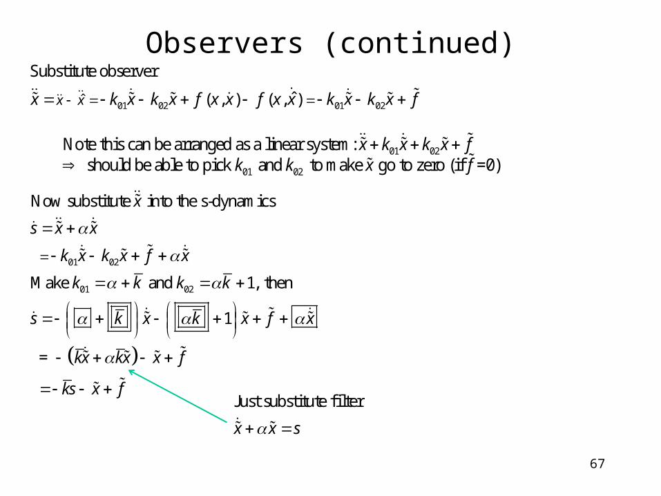
01 02 01 02
01 02
01 02
ˆ
Substitute observer
ˆ( , ) ( , )
Now substitute into the s-dynamics
Make and 1, then
x xx k x k x f x x f x x k x k x f
x
s x x
k x k x f x
k k k k
s k
1
=
x k x f x
kx kx x f
ks x f
Observers (continued)
01 02
01 02
Note this can be arranged as a linear system: should be able to pick and to make go to zero (if =0)
x k x k x fk k x f
Just substitute filter
x x s
68
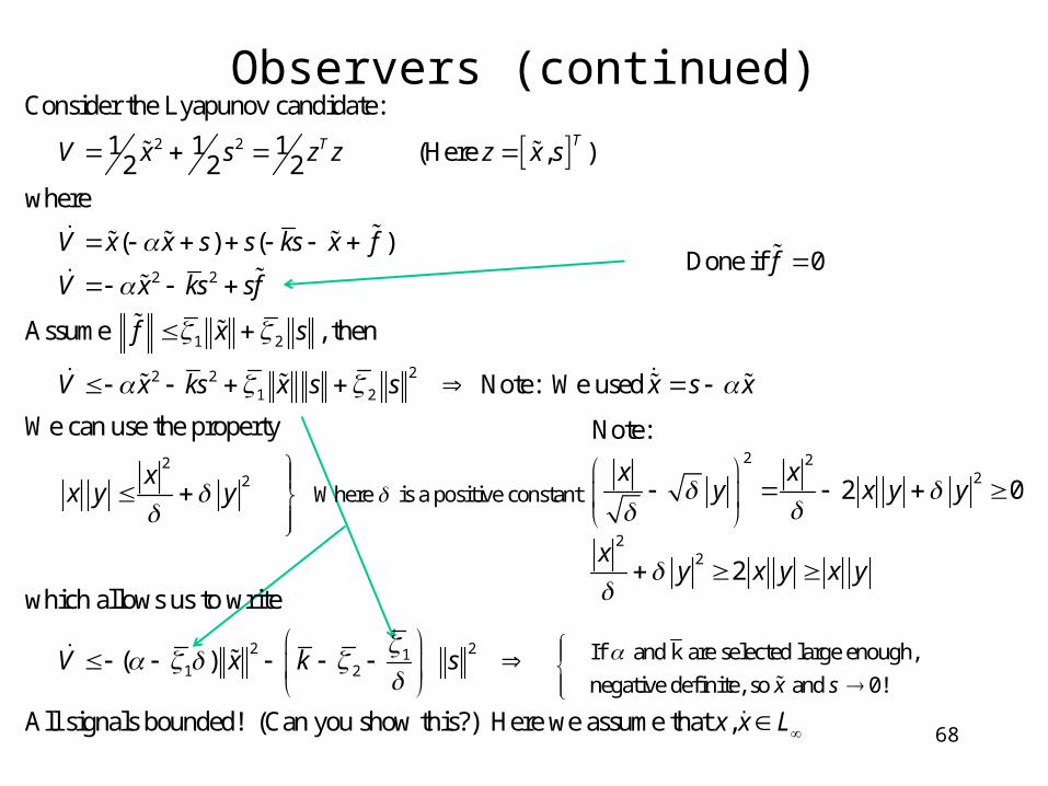
2 2
2 2
1 2
22 21 2
Consider the Lyapunov candidate:
1 1 1 (Here , )2 2 2where
( ) ( )
Assume , then
Note:
TTV x s z z z x s
V x x s s ks x f
V x ks sf
f x s
V x ks x s s
22
2 211 2
Where is a positive constant
We used
We can use the property
which allows us to write
( )
All signals bounded! (Can you show th
x s x
xx y y
V x k s
is?) Here we assume that , x x L
Observers (continued)
If and k are selected large enough,
negative definite, so and 0!x s
2 22
22
Note:
2 0
2
x xy x y y
xy x y x y
Done if 0 f
69
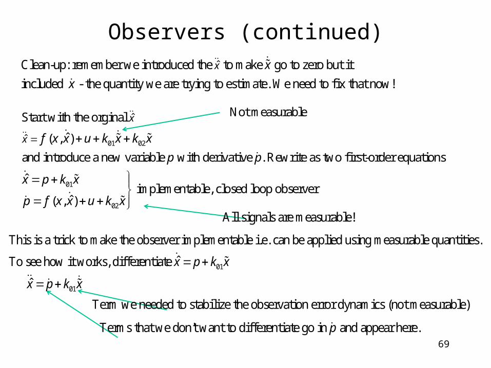
01 02
01
02
ˆ
ˆ
Start with the orginal
ˆ( , )
and introduce a new variable with derivative . Rewrite as two first-order equations
ˆimplementable, closed
ˆ( , )
x
x f x x u k x k x
p p
x p k x
p f x x u k x
loop observer
Observers (continued)ˆClean-up: remember we introduced the to make go to zero but it
included - the quantity we are trying to estimate. We need to fix that now!
x x
x
01
01
This is a trick to make the observer implementable i.e. can be applied using measurable quantities.
ˆTo see how it works, differentiate
ˆ
x p k x
x p k x
Not measurable
All signals are measurable!
Term we needed to stabilize the observation error dynamics (not measurable)
Terms that we don't want to differentiate go in and appear here.p
0
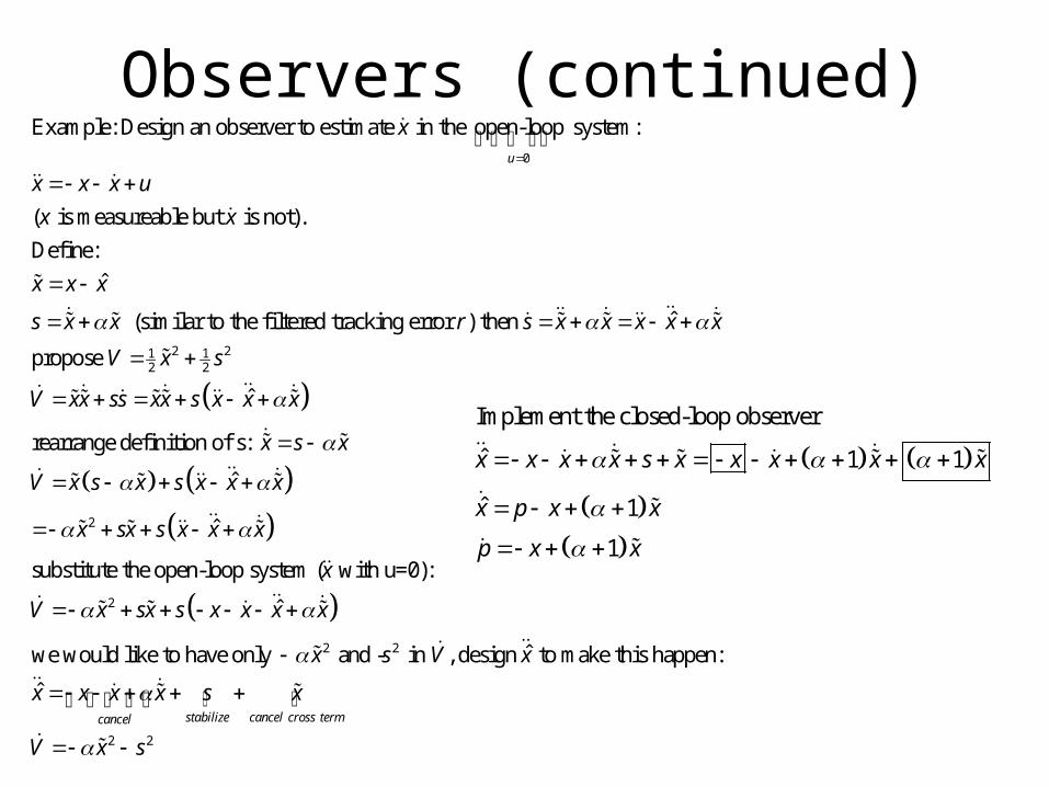
Example: Design an observer to estimate in the open-loop system:
( is measureable but is not).
Define:
ˆ
(similar to the filtered tracking error ) then
u
x
x x x u
x x
x x x
s x x r s x
2 21 12 2
2
ˆ
propose
ˆ
rearrange definition of s:
ˆ
ˆ
substitute the open-loop system ( with
x x x x
V x s
V xx ss xx s x x x
x s x
V x s x s x x x
x sx s x x x
x
2
2 2
2 2
u=0):
ˆ
ˆwe would like to have only and - in , design to make this happen:
ˆstabilize cancel cross termcancel
V x sx s x x x x
x s V x
x x x x s x
V x s
Observers (continued)
Implement the closed-loop observer
ˆ 1 1
ˆ 1
1
x x x x s x x x x x
x p x x
p x x
71
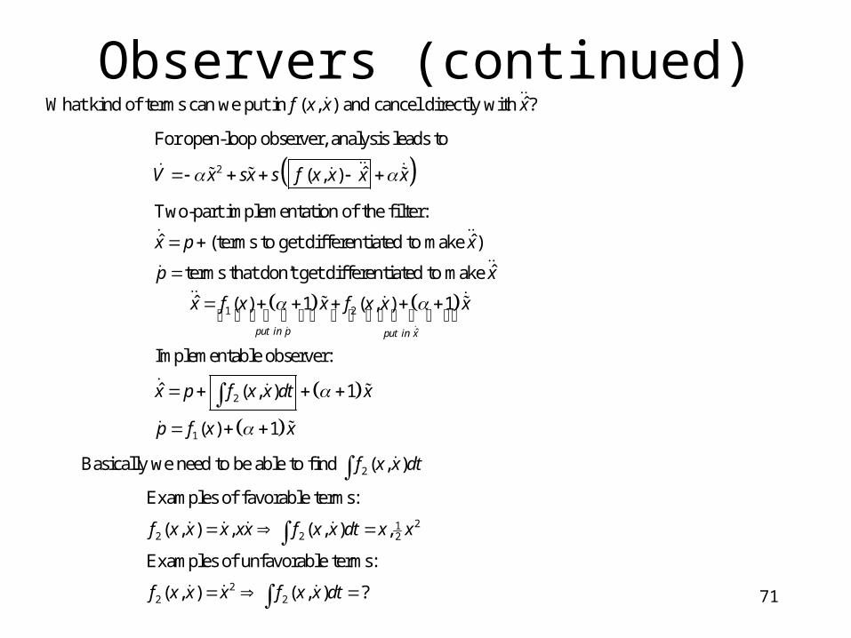
ˆWhat kind of terms can we put in ( , ) and cancel directly with ?f x x x
2
For open-loop observer, analysis leads to
ˆ( , )
Two-part implementation of the filter:
ˆ ˆ(terms to get differentiated to make )
terms that don't get differentiated to
V x sx s f x x x x
x p x
p
1 2
ˆ
2
1
ˆmake
ˆ ( ) 1 ( , ) 1
Implementable observer:
ˆ ( , ) 1
( ) 1
put in p put in x
x
x f x x f x x x
x p f x x dt x
p f x x
Observers (continued)
2Basically we need to be able to find ( , )f x x dt
212 2 2
22 2
Examples of favorable terms:
( , ) , ( , ) ,
Examples of unfavorable terms:
( , ) ( , ) ?
f x x x xx f x x dt x x
f x x x f x x dt
0
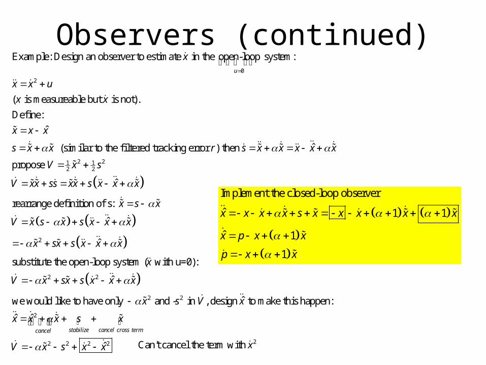
2
Example: Design an observer to estimate in the open-loop system:
( is measureable but is not).
Define:
ˆ
(similar to the filtered tracking error ) then
u
x
x x u
x x
x x x
s x x r s x
2 21 12 2
2
ˆ
propose
ˆ
rearrange definition of s:
ˆ
ˆ
substitute the open-loop system ( with u=
x x x x
V x s
V xx ss xx s x x x
x s x
V x s x s x x x
x sx s x x x
x
2 2
2 2
2
2 2 2 2
0):
ˆ
ˆwe would like to have only and - in , design to make this happen:
ˆ ˆ
ˆ
stabilize cancel cross termcancel
V x sx s x x x
x s V x
x x x s x
V x s x x
Observers (continued)
Implement the closed-loop observer
ˆ 1 1
ˆ 1
1
x x x x s x x x x x
x p x x
p x x
2Can't cancel the term with x
73
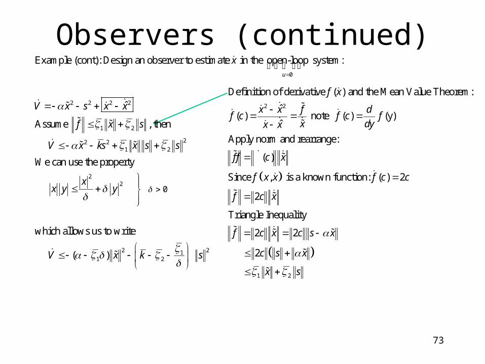
0
2 2 2 2
1 2
22 21 2
22
Example (cont): Design an observer to estimate in the open-loop system:
ˆ
Assume , then
We can use the property
u
x
V x s x x
f x s
V x ks x s s
xx y y
2 211 2
0
which allows us to write
( ) V x k s
Observers (continued)
2 2
Definition of derivative ( ) and the Mean Value Theorem:
ˆ( ) note ( ) (y)
ˆ
Apply norm and rearrange:
( )
Since , is a known function: ( ) 2
2
Triangle
f x
x x f df c f c f
x dyx x
f f c x
f x x f c c
f c x
1 2
Inequality
2 2
2
f c x c s x
c s x
x s
74
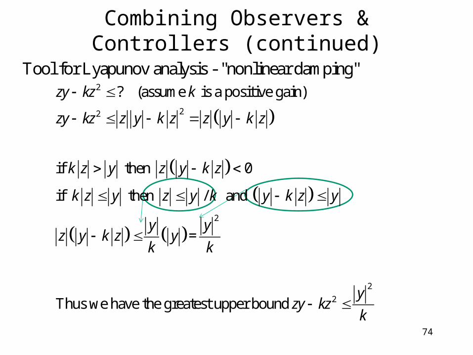
Combining Observers & Controllers (continued)
2
22
2
2
2
? (assume is a positive gain)
if then 0
if then / and
=
Thus we have the greatest upper bound
zy kz k
zy kz z y k z z y k z
k z y z y k z
k z y z y k y k z y
y yz y k z y
k k
yzy kz
k
Tool for Lyapunov analysis - "nonlinear damping"
75
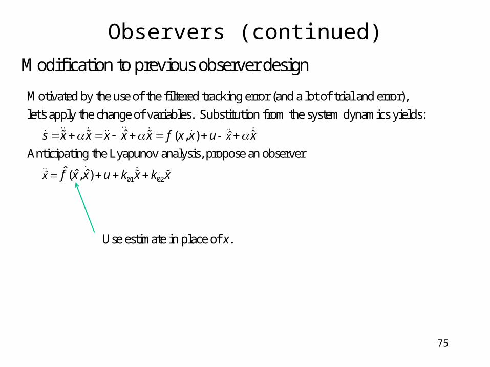
Observers (continued)
Modification to previous observer design
Use estimate in place of .x
Motivated by the use of the filtered tracking error (and a lot of trial and error),
let's apply the change of variables. Substitution from the system dynamics yields:
ˆ s x x x x x
01 02
ˆ
ˆ
( , )
Anticipating the Lyapunov analysis, propose an observer
ˆ ˆ ˆ ( , )
x
x
f x x u x
f x x u k x k x
x
76
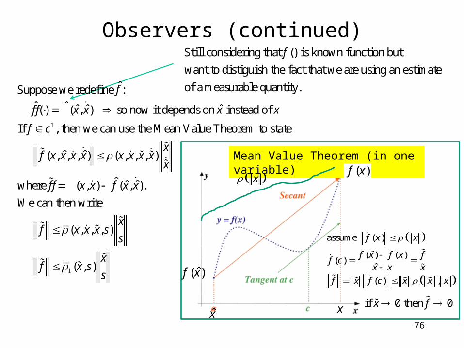
1
ˆSuppose we redefine :
ˆ ˆ ˆ ˆ ˆ ( ) ( , ) so now it depends on instead of
If , then we can use the Mean Value Theorem to state
ˆ ˆ ( , , , ) ( , , , )
ˆ ˆwhere ( , ) (
f
f f x x x x
f c
xf x x x x x x x x
x
f f x x f
1
ˆ, ).
We can then write
( , , , )
( , )
x x
xf x x x s
s
xf x s
s
Observers (continued)Still considering that () is known function but
want to distiguish the fact that we are using an estimate
of a measurable quantity.
f
( )f x
xx
ˆ( )f x
assume ( )
ˆ( ) ( )( )
ˆ
( ) ,
f x x
f x f x ff c
x x x
f x f c x x x
Mean Value Theorem (in one variable)
if 0 then 0x f
77
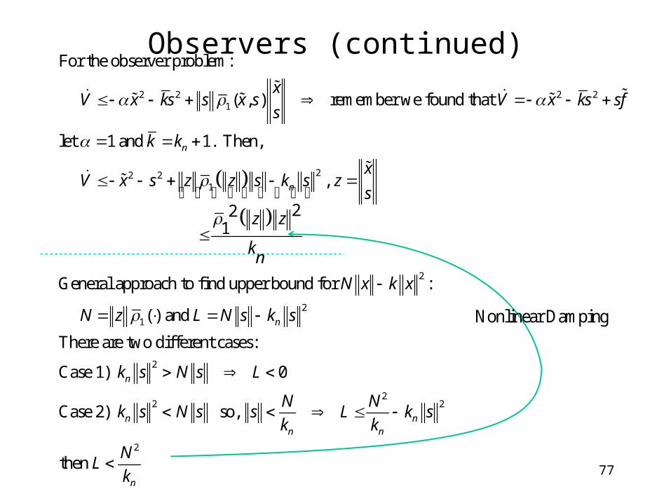
Observers (continued)
2 2 2 21
22 21
For the observer problem:
( , ) remember we found that
let 1 and 1. Then,
,
221
General approach to find
n
n
xV x ks s x s V x ks sf
s
k k
xV x s z z s k s z
s
z z
kn
2
2
1
2
22 2
2
upper bound for :
( ) and
There are two different cases:
Case 1) 0
Case 2) so,
then
n
n
n nn n
n
N x k x
N z L N s k s
k s N s L
N Nk s N s s L k s
k k
NL
k
Nonlinear Damping
78
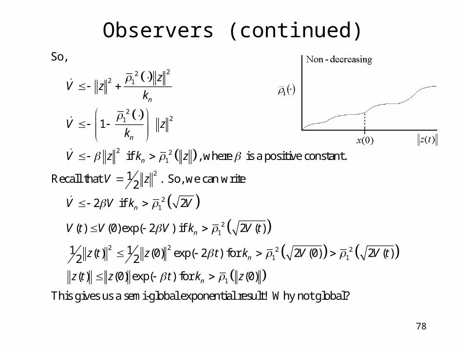
222 1
221
2 21
2
21
1
So,
1
if , where is a positive constant.
1Recall that . So, we can write2
2 if 2
( ) (0)exp( 2 ) if
n
n
n
n
n
zV z
k
V zk
V z k z
V z
V V k V
V t V V k
2
2 2 2 21 1
1
2 ( )
1 1 ( ) (0) exp( 2 ) for 2 (0) 2 ( )2 2
( ) (0) exp( ) for (0)
This gives us a semi-global exponential result! Why not global?
n
n
V t
z t z t k V V t
z t z t k z
Observers (continued)
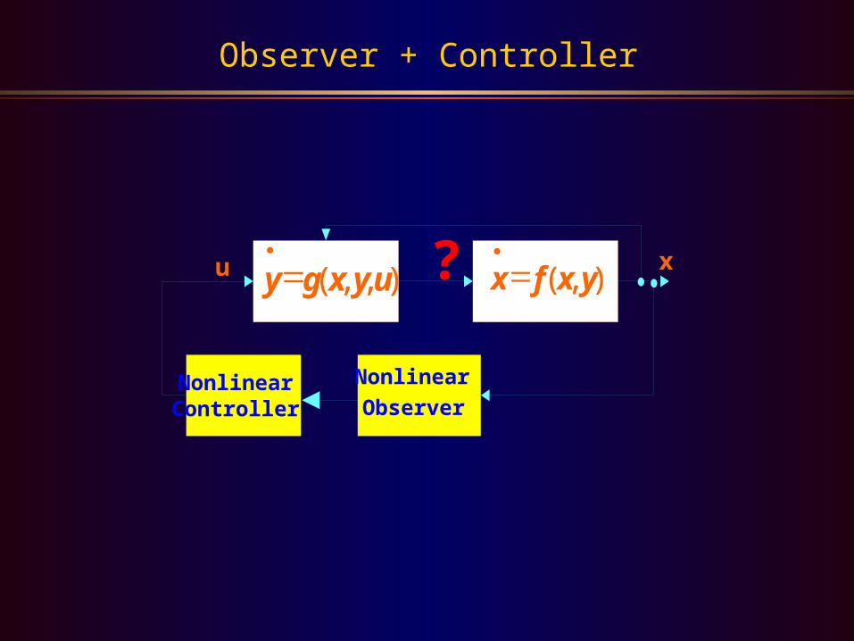
Observer + Controller
x f x y· ( , )y g x yu
·
= ( , , )u ? x
NonlinearController
Nonlinear
Observer
80
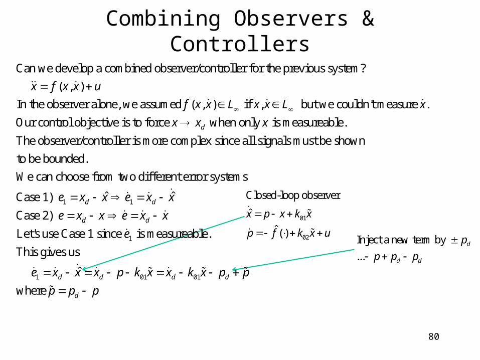
Combining Observers & Controllers
Can we develop a combined observer/controller for the previous system?
( , )
In the observer alone, we assumed ( , ) if , but we couldn't measure .
Our control objective is to
x f x x u
f x x L x x L x
1 1
force when only is measureable.
The observer/controller is more complex since all signals must be shown
to be bounded.
We can choose from two different error systems
ˆ ˆCase 1)
C
d
d d
x x x
e x x e x x
1
1 01 01
ase 2)
Let's use Case 1 since is measureable.
This gives us
ˆ
where
d d
d d d d
d
e x x e x x
e
e x x x p k x x k x p p
p p p
01
02
Closed-loop observer
ˆ
ˆ ( )
x p x k x
p f k x u
Inject a new term by
...d
d d
p
p p p
81
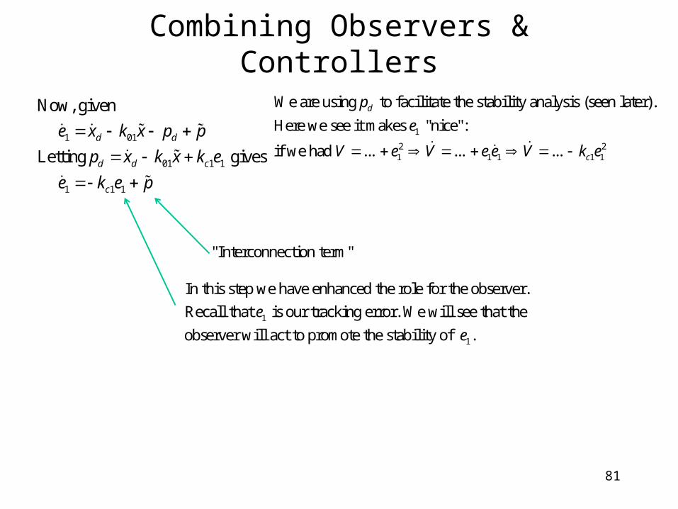
Combining Observers & Controllers
1
2 21 1 1 1 1
We are using to facilitate the stability analysis (seen later).
Here we see it makes "nice":
if we had ... ... ...
d
c
p
e
V e V e e V k e
1
1
In this step we have enhanced the role for the observer.
Recall that is our tracking error. We will see that the
observer will act to promote the stability of .
e
e
1 01
01 1 1
1 1 1
Now, given
Letting gives
d d
d d c
c
e x k x p p
p x k x k e
e k e p
"Interconnection term"
82
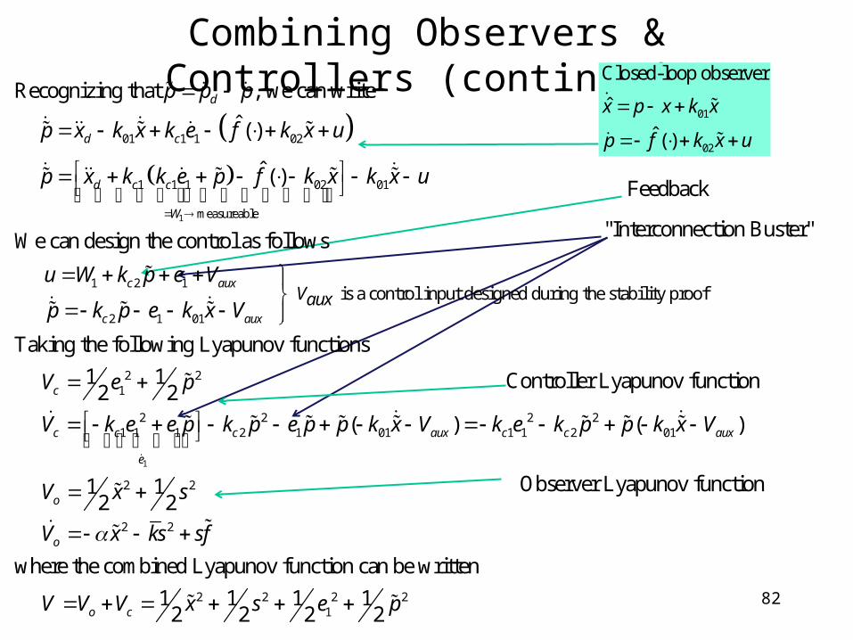
Combining Observers & Controllers (continued)
1
01 1 1 02
1 1 1 02 01
measureable
Recognizing that , we can write
ˆ ( )
ˆ ( )
We can design the control as follows
d
d c
d c c
W
p p p
p x k x k e f k x u
p x k k e p f k x k x u
1 2 1
2 1 01
2 21
21 1 1
is a control input designed during the stability proof
Taking the following Lyapunov functions
1 1 2 2
c aux
c aux
c
c c
Vauxu W k p e V
p k p e k x V
V e p
V k e e p
1
2 2 22 1 01 1 1 2 01
2 2
2 2
2 2 2 21
( ) ( )
1 1 2 2
where the combined Lyapunov function can be written
1 1 1 1 2 2 2 2
c aux c c aux
e
o
o
o c
k p e p p k x V k e k p p k x V
V x s
V x ks sf
V V V x s e p
Feedback
"Interconnection Buster"
Observer Lyapunov function
01
02
Closed-loop observer
ˆ
ˆ ( )
x p x k x
p f k x u
Controller Lyapunov function
83
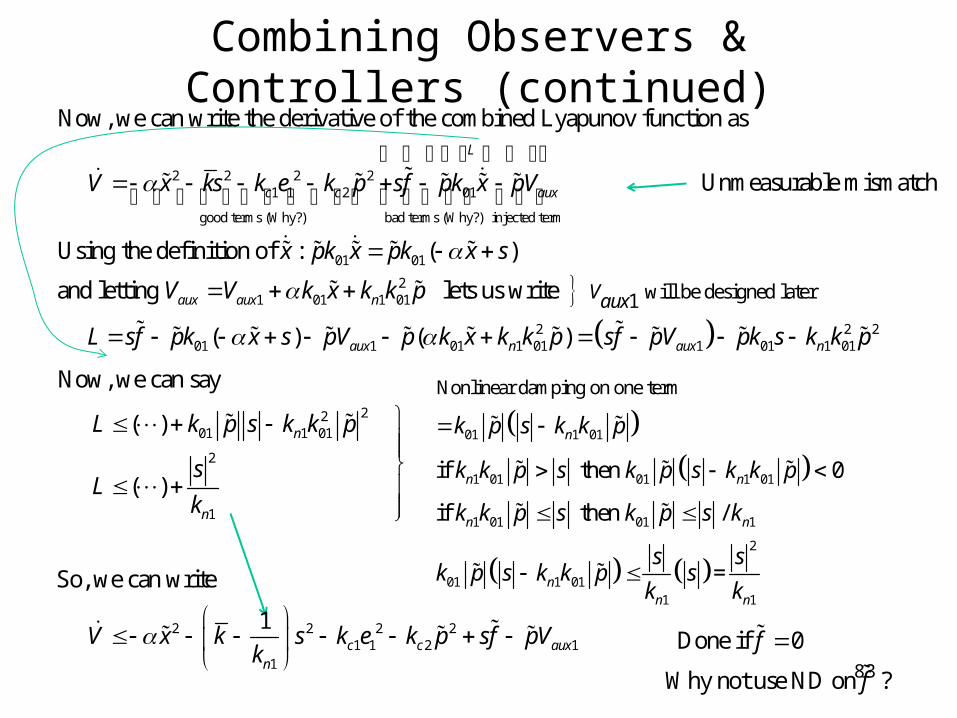
Combining Observers & Controllers (continued)
2 2 2 21 1 2 01
good terms (Why?) bad terms (Why?) injected term
Now, we can write the derivative of the combined Lyapunov function as
Using
L
c c auxV x ks k e k p sf pk x pV
01 01
21 01 1 01
201 1 01 1 01 1
will be designed later1
the definition of : ( )
and letting lets us write
( ) ( )
aux aux n
aux n aux
Vaux
x pk x pk x s
V V k x k k p
L sf pk x s pV p k x k k p sf pV pk
2 201 1 01
2201 1 01
2
1
2 2 2 21 1 2 1
1
Now, we can say
( )
( )
So, we can write
1
n
n
n
c c auxn
s k k p
L k p s k k p
sL
k
V x k s k e k p sf pVk
Unmeasurable mismatch
01 1 01
1 01 01 1 01
1 01 01 1
2
01 1 011 1
Nonlinear damping on one term
if then 0
if then /
=
n
n n
n n
nn n
k p s k k p
k k p s k p s k k p
k k p s k p s k
s sk p s k k p s
k k
Done if 0
Why not use ND on ?
f
f
84
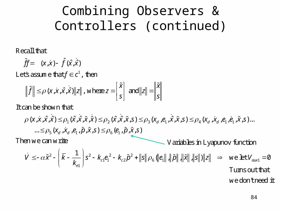
Combining Observers & Controllers (continued)
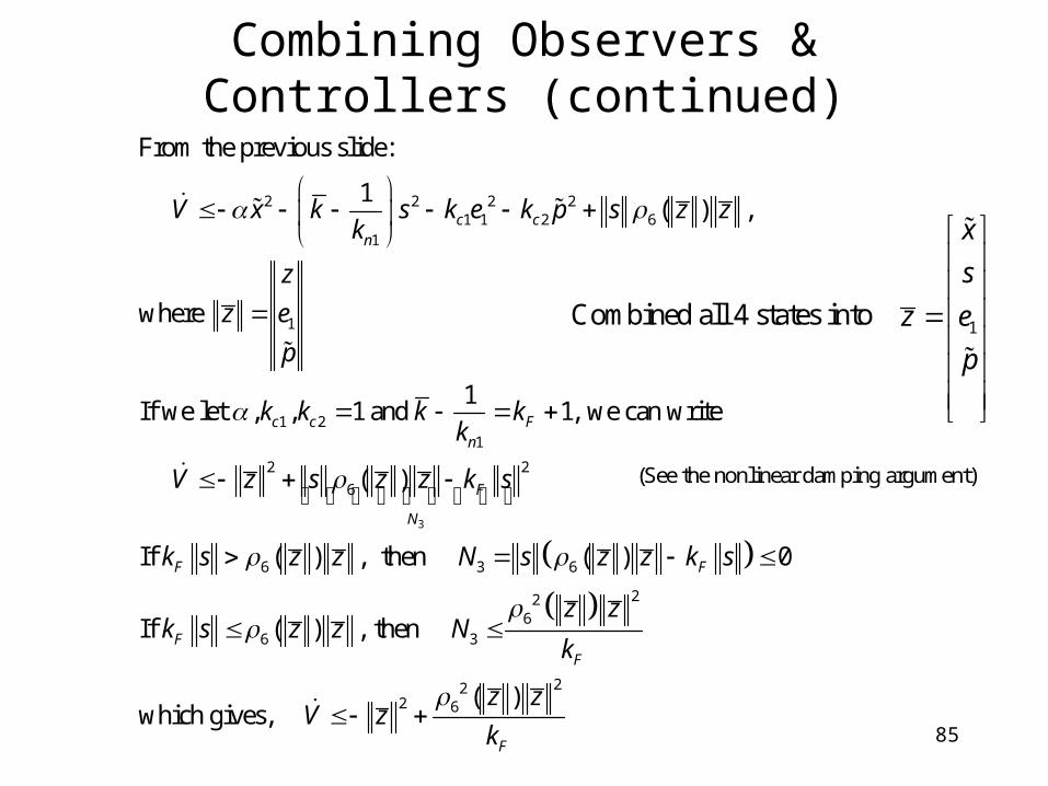
1
1 2 3 1
Recall that
ˆ ˆ ˆ ( , ) ( , )
Let's assume that , then
ˆ ˆ ( , , , ) , where and
It can be shown that
ˆ ˆ ˆ ˆ ˆ ˆ ˆ ( , , , ) ( , , , ) ( , , , ) ( , ,d
f f x x f x x
f c
x xf x x x x z z z
s s
x x x x x x x x x x x s x e
4 1 1
5 1 6 1
2 2 2 21 1 2 6 1 1
1
, , ) ( , , , , , )...
... ( , , , , , ) ( , , , )
Then we can write
1 ( , , , ) we let 0
d d
d d
c c auxn
x x s x x e e x s
x x e p x s e p x s
V x k s k e k p s e p x s z Vk
Variables in Lyapunov function
Turns out that
we don't need it
85
Combining Observers & Controllers (continued)
3
2 2 2 21 1 2 6
1
1
1 21
2 2
6
6
From the previous slide:
1 ( ) ,
where
1If we let , , 1 and 1, we can write
( )
If ( ) , then
c cn
c c Fn
F
N
F
V x k s k e k p s z zk
z
z e
p
k k k kk
V z s z z k s
k s z z
3 6
226
6 3
222 6
( ) 0
If ( ) , then
( )which gives,
F
FF
F
N s z z k s
z zk s z z N
k
z zV z
k
(See the nonlinear damping argument)
1
x
s
z e
p
Combined all 4 states into
86
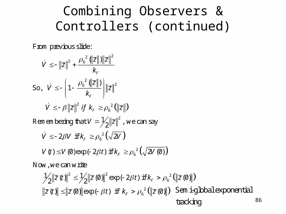
Combining Observers & Controllers (continued)
222 6
226
2 26
2
26
26
From previous slide:
( )
( )So, 1
1Remembering that , we can say2
2 if 2
( ) (0)exp( 2 ) if 2 (0)
Now, we
F
F
F
F
F
z zV z
k
zV z
k
V z if k z
V z
V V k V
V t V t k V
2 2 26
26
can write
1 1 ( ) (0) exp( 2 ) if (0)2 2
( ) (0) exp( ) if (0)
F
F
z t z t k z
z t z t k z
Semi-global exponential
tracking
87
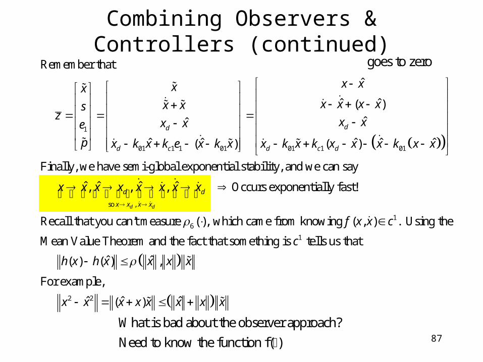
Combining Observers & Controllers (continued)
1
01 1 1 01 01 1 01
Remember that
ˆ
ˆ ˆ( ) ˆˆ
ˆ ˆ ˆ ˆ ˆ( ) ( )
Finally, we have semi-global exponent
dd
d c d c d
x xxxx x x xx xs
zx xx xe
p x k x k e x k x x k x k x x x k x x
so ,
16
ial stability, and we can say
ˆ ˆ ˆ ˆ , , , Occurs exponentially fast!
Recall that you can't measure ( ), which came from knowing ( , ) . Using t
d d
d d
x x x x
x x x x x x x x
f x x c
1
2 2
he
Mean Value Theorem and the fact that something is tells us that
ˆ ˆ ( ) ( ) ,
For example,
ˆ ˆ ˆ ( )
c
h x h x x x x
x x x x x x x x
goes to zero
What is bad about the observer approach?
Need to know the function f( )
88
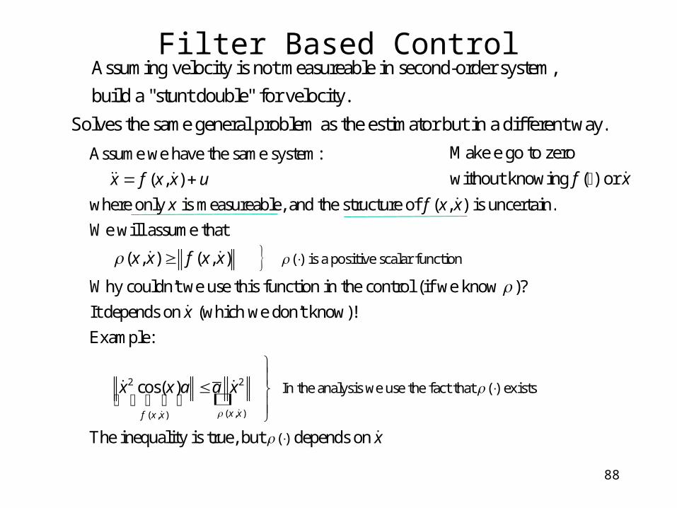
Filter Based Control
( ) is a positive scalar functio
Assume we have the same system:
( , )
where only is measureable, and the structure of ( , ) is uncertain.
We will assume that
( , ) ( , )
x f x x u
x f x x
x x f x x
2 2
( , )( , )
n
In the analysis we use the fact that
Why couldn't we use this function in the control (if we know )?
It depends on (which we don't know)!
Example:
cos( )
x xf x x
x
x x a a x
( ) exists
( )The inequality is true, but depends on x
Assuming velocity is not measureable in second-order system,
build a "stunt double" for velocity.
Make e go to zero
without knowing ( ) or f x
Solves the same general problem as the estimator but in a different way.
89
Filtering Control (continued)
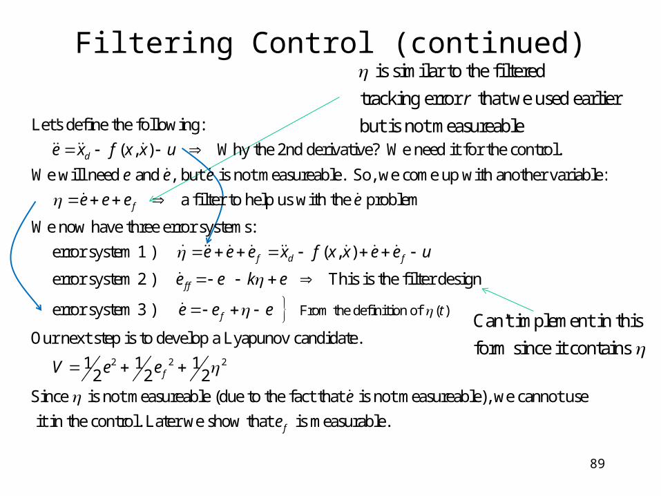
Let's define the following:
( , ) Why the 2nd derivative? We need it for the control.
We will need and , but is not measureable. So, we come up with another variable:
de x f x x u
e e e
a filter to help us with the problem
We now have three error systems:
error system 1 ) ( , )
error system 2 ) This is the
f
f d f
f f
e e e e
e e e x f x x e e u
e e k e
2 2 2
From the definition of ( )
filter design
error system 3 )
Our next step is to develop a Lyapunov candidate.
1 1 1 2 2 2Since is not measureable (due to the fact th
f
f
te e e
V e e
at is not measureable), we cannot use
it in the control. Later we show that is measurable.f
e
e
is similar to the filtered
tracking error that we used earlier
but is not measureable
r
Can't implement in this
form since it contains
90
Filtering Control (continued)
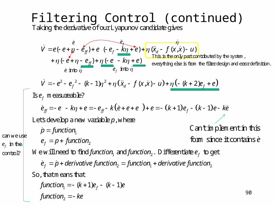
2 2 2
Taking the derivative of our Lyapunov candidate gives
( ) ( ) ( ( , ) )
( ) ( )
( 1) ( , ) ( 2)
Is measurea
f f f d
f f
f d f
f
V e e e e e k e x f x x u
e e e k e
V e e k x f x x u k e e
e
1
2
1 2
ble?
1 1
Let's develop a new variable , where
We will need to find and . Differentiate to get
f f f f f
f
f
e e k e e k e e e e k e k e ke
p
p function
e p function
function function e
2 1 2
1
2
So, that means that
( 1) ( 1)
f
f
e p derivative function function derivative function
function k e k e
function ke
This is the only part contributed by the system,
everything else is from the filter design and error definition.
fe e
into fe into e
can we use
in the
control?
fe
Can't implement in this
form since it contains e
91
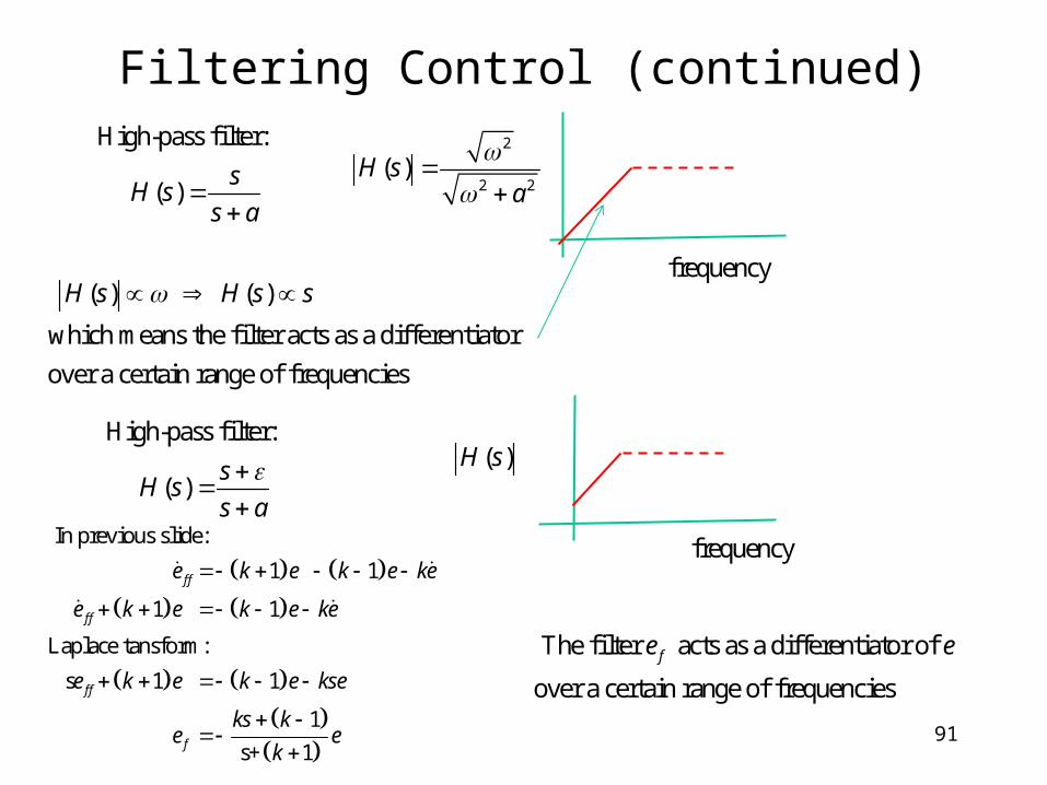
Filtering Control (continued)
In previous slide:
1 1
1 1
Laplace tansform:
s 1 1
1
s+ 1
f f
f f
f f
f
e k e k e ke
e k e k e ke
e k e k e kse
ks ke e
k
High-pass filter:
( )s
H ss a
frequency
2
2 2 ( )H s
a
( ) ( )
which means the filter acts as a differentiator
over a certain range of frequencies
H s H s s
High-pass filter:
( )s
H ss a
frequency
( )H s
The filter acts as a differentiator of
over a certain range of frequencies
fe e
92
Filtering Control (continued)
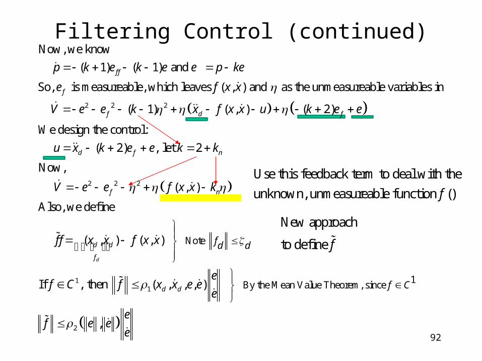
2 2 2
Now, we know
( 1) ( 1) and
So, is measureable, which leaves ( , ) and as the unmeasureable variables in
( 1) ( , ) ( 2)
We design the contro
f f
f
f d f
p k e k e e p ke
e f x x
V e e k x f x x u k e e
2 2 2
11
Note
By the Mean Value Theo
l:
( 2) , let 2
Now,
( , )
Also, we define
( , ) ( , )
If , then ( , , , )
d
d f n
f n
d d
f
d d
fd d
u x k e e k k
V e e f x x k
f f x x f x x
ef C f x x e e
e
2
1rem, since
,
f C
ef e e
e
Use this feedback term to deal with the
unknown, unmeasureable function ()f
New approach
to define f
93
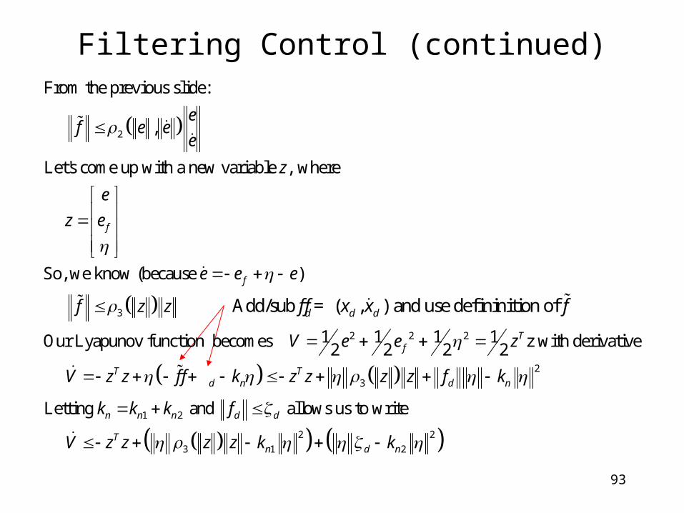
Filtering Control (continued)
2
3
From the previous slide:
,
Let's come up with a new variable , where
So, we know (because )
1Our Lyapunov function becomes
f
f
ef e e
e
z
e
z e
e e e
f z z
V
2 2 2
2
3
1 2
2 2
3 1 2
1 1 1 z with derivative2 2 2 2
Letting and allows us to write
Tf
T Td n d n
n n n d d
Tn d n
e e z
V z z f f k z z z z f k
k k k f
V z z z z k k
Add/sub = ( , ) and use defininition of d d df f x x f
94
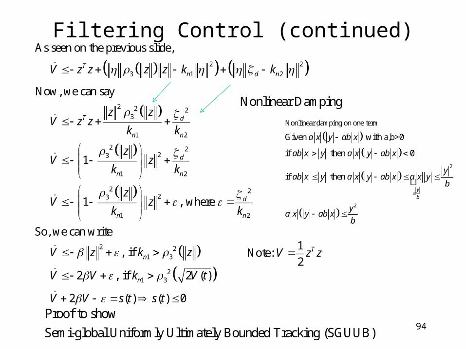
2 2
3 1 2
2 2 23
1 2
2 223
1 2
2 223
1 2
As seen on the previous slide,
Now, we can say
1
1 , where
So, we can
Tn d n
T d
n n
d
n n
d
n n
V z z z z k k
z zV z z
k k
zV z
k k
zV z
k k
2 21 3
21 3
write
, if
2 , if 2 ( )
2 ( ) ( ) 0
n
n
V z k z
V V k V t
V V s t s t
Filtering Control (continued)
Nonlinear Damping
1 Note:
2TV z z
Proof to show
Semi-global Uniformly Ultimately Bounded Tracking (SGUUB)
2
2
Nonlinear damping on one term
Given with a,b>0
if then 0
if then y
b
a x y ab x
ab x y a x y ab x
yab x y a x y ab x a x y
b
ya x y ab x
b
95
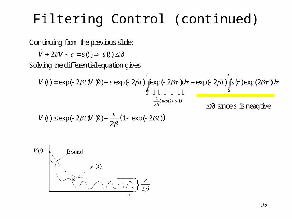
Filtering Control (continued)
0 0
1exp(2 1
2
Continuing from the previous slide:
2 ( ) ( ) 0
Solving the differential equation gives
( ) exp( 2 ) (0) exp( 2 ) exp( 2 ) exp( 2 ) ( ) exp(2 )
(
t t
t
V V s t s t
V t t V t d t s d
V
) exp( 2 ) (0) 1 exp( 2 )2
t t V t
0 since is neagtives
96
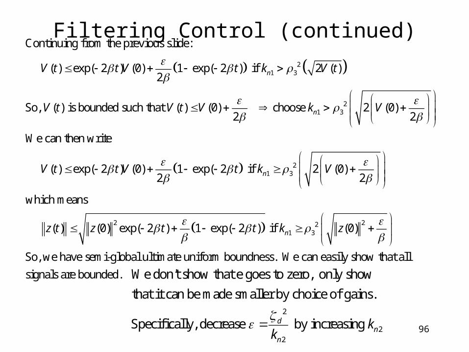
Filtering Control (continued)
21 3
21 3
Continuing from the previous slide:
( ) exp( 2 ) (0) 1 exp( 2 ) if 2 ( )2
So, ( ) is bounded such that ( ) (0) choose 2 (0)2 2
We can then write
( ) e
n
n
V t t V t k V t
V t V t V k V
V t
21 3
2 221 3
xp( 2 ) (0) 1 exp( 2 if 2 (0)2 2
which means
( ) (0) exp( 2 ) 1 exp( 2 ) if (0)
So, we have semi-global ultimate uniform boundness. We can easily
n
n
t V t k V
z t z t t k z
show that all
signals are bounded.
2
22
We don't show that e goes to zero, only show
that it can be made smaller by choice of gains.
Specifically, decrease by increasing dn
n
kk
97
Adaptive Approach
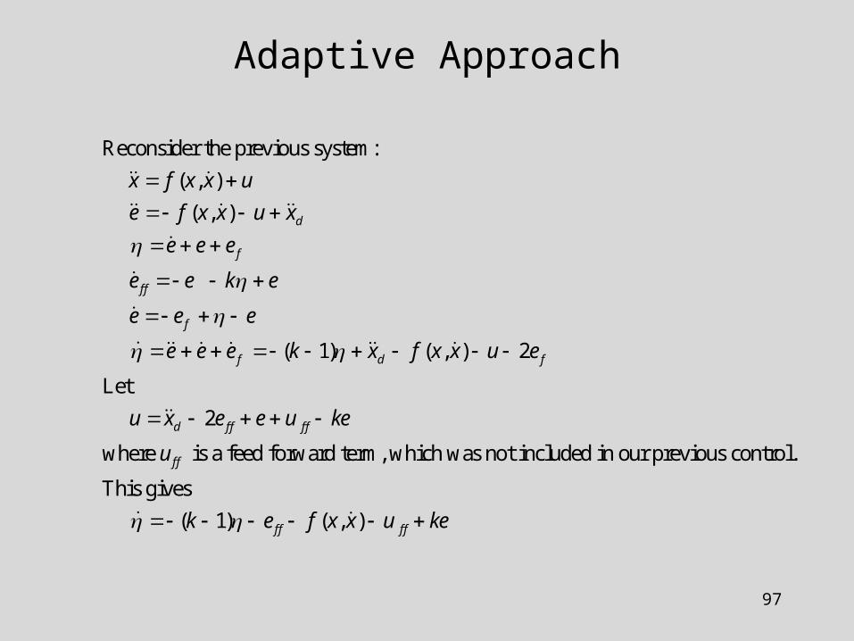
Reconsider the previous system:
( , )
( , )
( 1) ( , ) 2
Let
2
where
d
f
f f
f
f d f
d f ff f
x f x x u
e f x x u x
e e e
e e k e
e e e
e e e k x f x x u e
u x e e u ke
u
is a feed forward term, which was not included in our previous control.
This gives
( 1) ( , )
ff
f ff fk e f x x u ke
98
Adaptive Approach (continued)
2
2 2 2
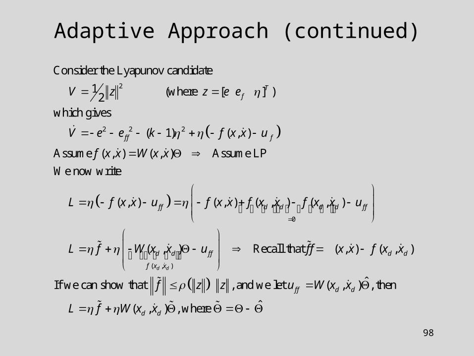
Consider the Lyapunov candidate
1 (where [ ] )2which gives
( 1) ( , )
Assume ( , ) ( , ) Assume LP
We now write
( , ) (
Tf
f ff
ff
V z z e e
V e e k f x x u
f x x W x x
L f x x u f x
0
( , )
, ) ( , ) ( , )
( , ) Recall that ( , ) ( , )
ˆIf we can show that , and we let ( , ) , then
d d
d d d d ff
d d ff d d
f x x
ff d d
x f x x f x x u
L f W x x u f f x x f x x
f z z u W x x
ˆ ( , ) , where d dL f W x x
99
Adaptive Approach (continued)
2 2 2
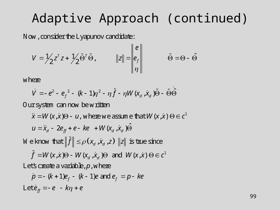
Now, consider the Lyapunov candidate:
ˆ1 1 , 2 2
where
ˆ ( 1) ( , )
Our system can now be written
( , ) , whe
T Tf
f d d
e
V z z z e
V e e k f W x x
x W x x u
1
1
re we assume that ( , )
ˆ 2 ( , )
We know that , , is true since
( , ) ( , ) and ( , )
Let's create a variable, , where
( 1)
d f f d d
d d
d d
f
W x x c
u x e e ke W x x
f x x z z
f W x x W x x W x x c
p
p k e
( 1) and
Let
f
f f
k e e p ke
e e k e
100
Adaptive Approach (continued)
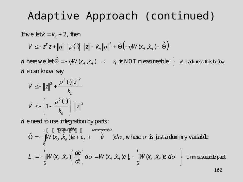
2
222
2
We address this below
If we let 2, then
ˆ ( , )
ˆWhere we let ( , ) is NOT measureable!
We can know say
( )
1
n
Tn d d
d d
n
n
k k
V z z z k W x x
W x x
zV z
k
Vk
2
0
1 0
0 0
We need to use integration by parts:
ˆ ( , )( ) , where is just a dummy variable
( , ) ( , ) | ( , )
unmeasurablet
d d f
tt
d d d d d d
measurable
z
W x x e e e d
deL W x x d W x x e W x x e d
dt
Unmeasurable part t
101
Adaptive Approach (continued)
1 0
0
1
0
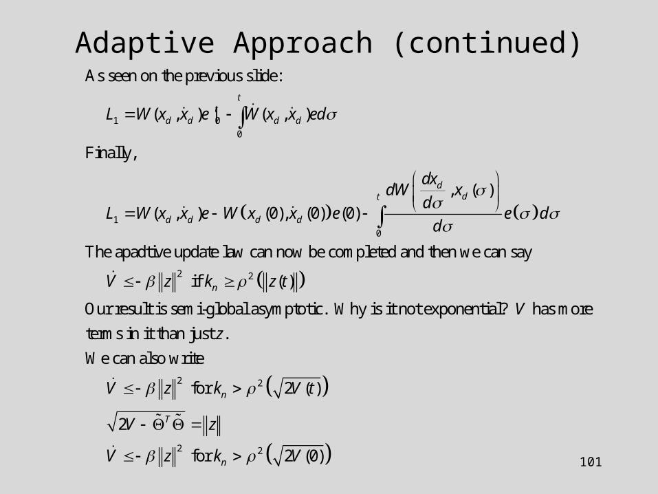
As seen on the previous slide:
( , ) | ( , )
Finally,
, ( )
( , ) (0), (0) (0)
The apadtive update law can now be completed and then we ca
tt
d d d d
ddt
d d d d
L W x x e W x x ed
dxdW x
dL W x x e W x x e e d
d
2 2
2 2
n say
if ( )
Our result is semi-global asymptotic. Why is it not exponential? has more
terms in it than just .
We can also write
for 2 ( )
2
n
n
T
V z k z t
V
z
V z k V t
V z
V
2 2 for 2 (0)nz k V
102
Adaptive Approach (continued)
2 2
t
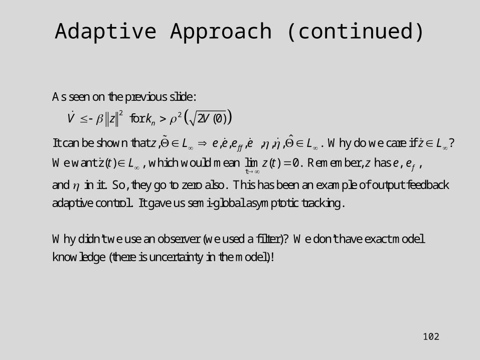
As seen on the previous slide:
for 2 (0)
ˆIt can be shown that , , , , , , , . Why do we care if ?
We want z( ) , which would mean lim ( ) 0. Remember, h
n
f f
V z k V
z L e e e e L z L
t L z t z
as , ,
and in it. So, they go to zero also. This has been an example of output feedback
adaptive control. It gave us semi-global asymptotic tracking.
Why didn't we use an observer (we used a fi
fe e
lter)? We don't have exact model
knowledge (there is uncertainty in the model)!
103
Variable Structure Observer
1
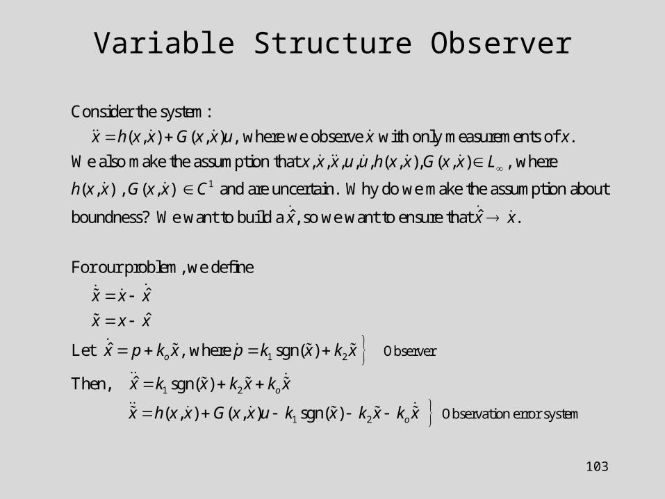
Consider the system:
( , ) ( , ) , where we observe with only measurements of .
We also make the assumption that , , , , , ( , ), ( , ) , where
( , ) , ( , ) and are un
x h x x G x x u x x
x x x u u h x x G x x L
h x x G x x C
1
certain. Why do we make the assumption about
ˆ ˆboundness? We want to build a , so we want to ensure that .
For our problem, we define
ˆ
ˆ
ˆLet , where sgno
x x x
x x x
x x x
x p k x p k
2
1 2
1 2
Observer
Observation error system
( )
ˆThen, sgn( )
( , ) ( , ) sgn( )
o
o
x k x
x k x k x k x
x h x x G x x u k x k x k x
104
Variable Structure Observer (continued)
1 2
2 0
1 2
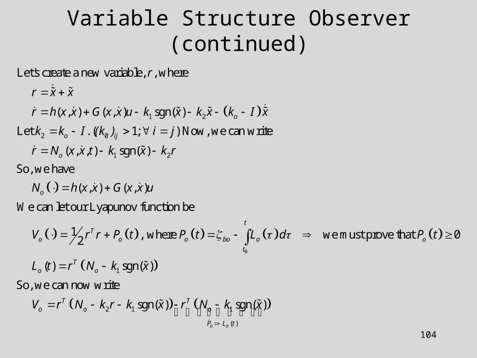
Let's create a new variable, , where
( , ) ( , ) sgn( )
Let . ( 1; ) Now, we can write
( , , ) sgn( )
So, we have
o
o ij
o
o
r
r x x
r h x x G x x u k x k x k I x
k k I (k ) i j
r N x x t k x k r
N h
0
1
2 1
( , ) ( , )
We can let our Lyapunov function be
1 , where we must prove that 02
( ) sgn( )
So, we can now write
sgn( )
tT
o o o bo o o
t
To o
T To o o
x x G x x u
V r r P t P t L d P t
L t r N k x
V r N k r k x r N k
1
( )
sgn( )
o oP L t
x
105
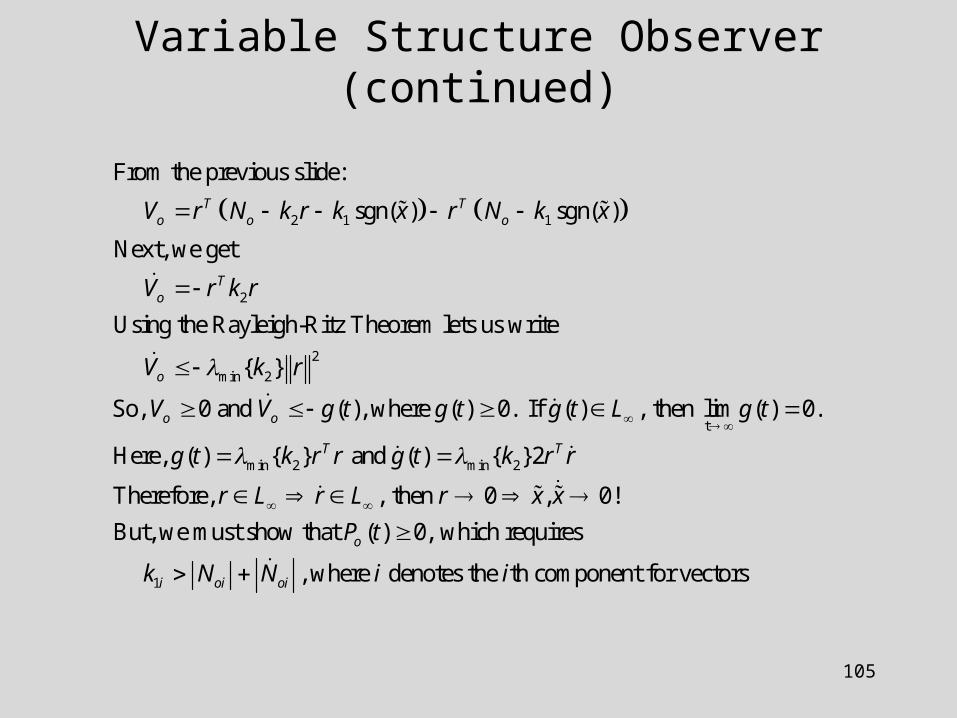
Variable Structure Observer (continued)
2 1 1
2
2
min 2
From the previous slide:
sgn( ) sgn( )
Next, we get
Using the Rayleigh-Ritz Theorem lets us write
{ }
So, 0 and ( ), where ( ) 0. If
T To o o
To
o
o o
V r N k r k x r N k x
V r k r
V k r
V V g t g t
t
min 2 min 2
1
( ) , then lim ( ) 0.
Here, ( ) { } and ( ) { }2
Therefore, , then 0 , 0!
But, we must show that ( ) 0, which requires
, where denotes the
T T
o
i oi oi
g t L g t
g t k r r g t k r r
r L r L r x x
P t
k N N i i
th component for vectors
106
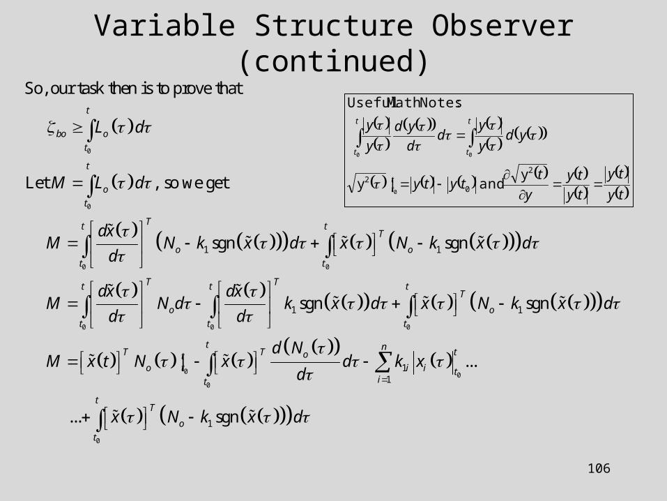
Variable Structure Observer (continued)
0
0
0 0
0 0
1 1
1
So, our task then is to prove that
Let , so we get
sgn sgn
sgn
t
bo o
t
t
o
t
Tt tT
o o
t t
T Tt t
o
t t
L d
M L d
dxM N k x d x N k x d
d
dx dxM N d k x d x
d d
0
0 0
0
0
1
11
1
sgn
| ...
... sgn
tT
o
t
t nT T tot
o t i i tit
tT
o
t
N k x d
d NM x t N x d k x
d
x N k x d
ty
ty
ty
ty
y
ttyty
ydy
yd
d
yd
y
y
tt
t
t
t
t
2
02 y
and |y
:NotesMath Useful
0
00
107
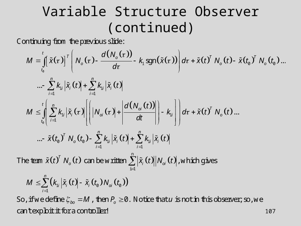
Variable Structure Observer (continued)
0
1 0 0
1 11 1
1 11
Continuing from the previous slide:
sgn ...
...
tT T To
o o o
t
n n
i i i ii i
noi
i i oi ii
d NM x N k x d x t N t x t N t
d
k x t k x t
d N tM k x N k
dt
0
0 0 1 11 1
n
i 1
1 0 01
...
...
The term can be written , which gives
So, if we define , then 0. Notice t
tT
o
t
n nT
o i i i ii i
T
o i oi
n
i i i oii
bo o
d x t N t
x t N t k x t k x t
x t N t x t N t
M k x t x t N t
M P
hat is not in this observer; so, we
can't exploit it for a controller!
u
108
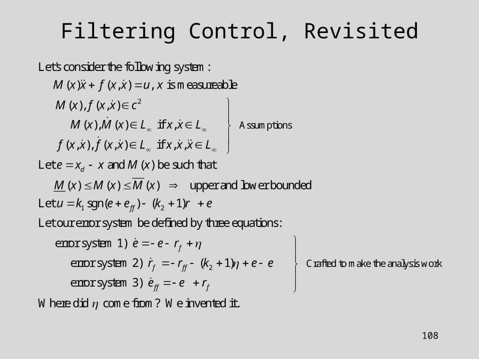
Filtering Control, Revisited
2
Assumptions
Let's consider the following system:
( ) ( , ) , is measureable
( ), ( , )
( ), ( ) if ,
( , ), ( , ) if , ,
Let and ( ) d
M x x f x x u x
M x f x x c
M x M x L x x L
f x x f x x L x x x L
e x x M x
1 2
be such that
( ) ( ) ( ) upper and lower bounded
Let sgn( ) ( 1)
Let our error system be defined by three equations:
error system 1)
error system 2)
f f
f
f
M x M x M x
u k e e k r e
e e r
r r
2 Crafted to make the analysis work( 1)
error system 3)
Where did come from? We invented it.
f f
f f f
k e e
e e r
109
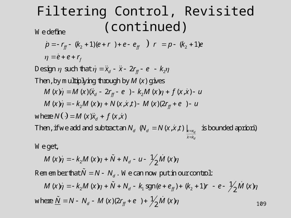
Filtering Control, Revisited (continued)
2 2
2
2
We define
( 1)( ) ( 1)
Design such that 2
Then, by multiplying through by ( ) gives
( ) ( )( 2 ) ( ) ( , )
f f f f
f
d f f
d f f
p r k e r e e r p k e
e e r
x x r e k
M x
M x M x x r e k M x f x x u
2
2
( ) ( ) ( , , ) ( )(2 )
where ( ) ( , )
Then, if we add and subtract an ( ( , , ) | is bounded apriori)
We get,
1 ( ) ( ) ( )2
Remembe
d
d
f f
d
d d x x
x x
d
M x k M x N x x t M x r e u
N M x x f x x
N N N x x t
M x k M x N N u M x
2 1 2
r that . We can now put in our control:
1 ( ) ( ) sgn( ) ( 1) ( )21where ( )(2 ) ( )2
d
d f f
d f f
N N N
M x k M x N N k e e k r e M x
N N N M x r e M x
110
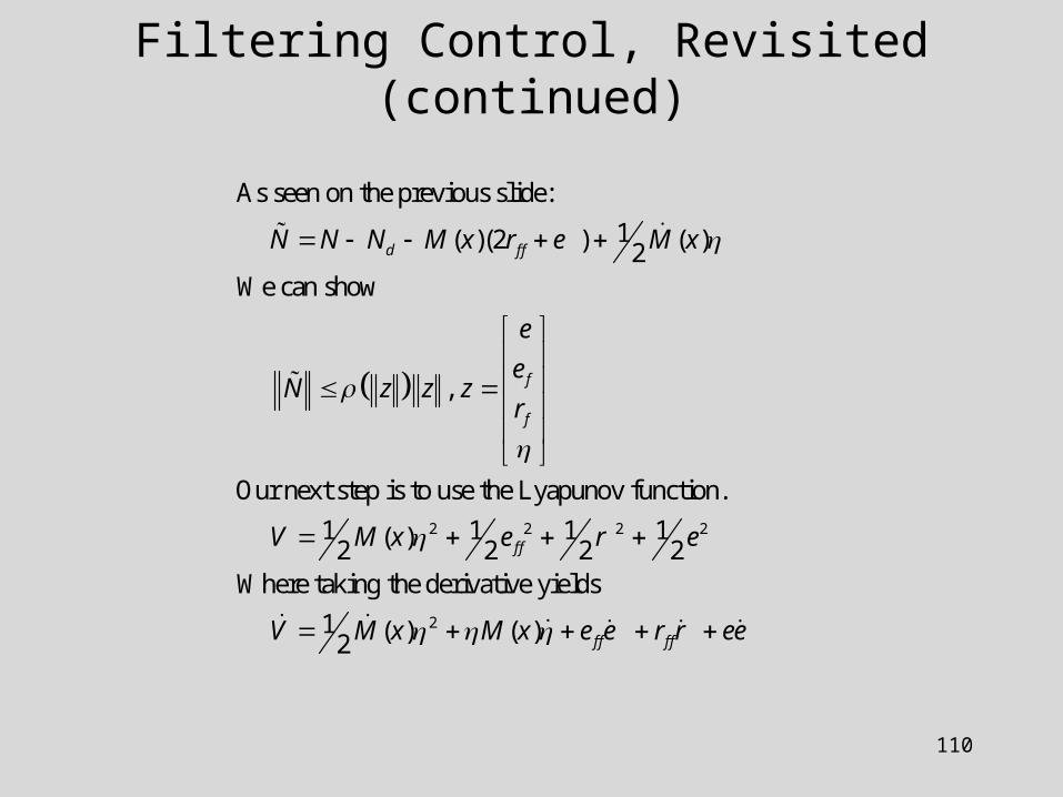
Filtering Control, Revisited (continued)
2 2 2 2
As seen on the previous slide:
1 ( )(2 ) ( )2We can show
,
Our next step is to use the Lyapunov function.
1 1 1 1 ( )2 2 2 2Where taking
d f f
f
f
f f
N N N M x r e M x
e
eN z z z
r
V M x e r e
2
the derivative yields
1 ( ) ( )2 f f f fV M x M x e e r r ee
111
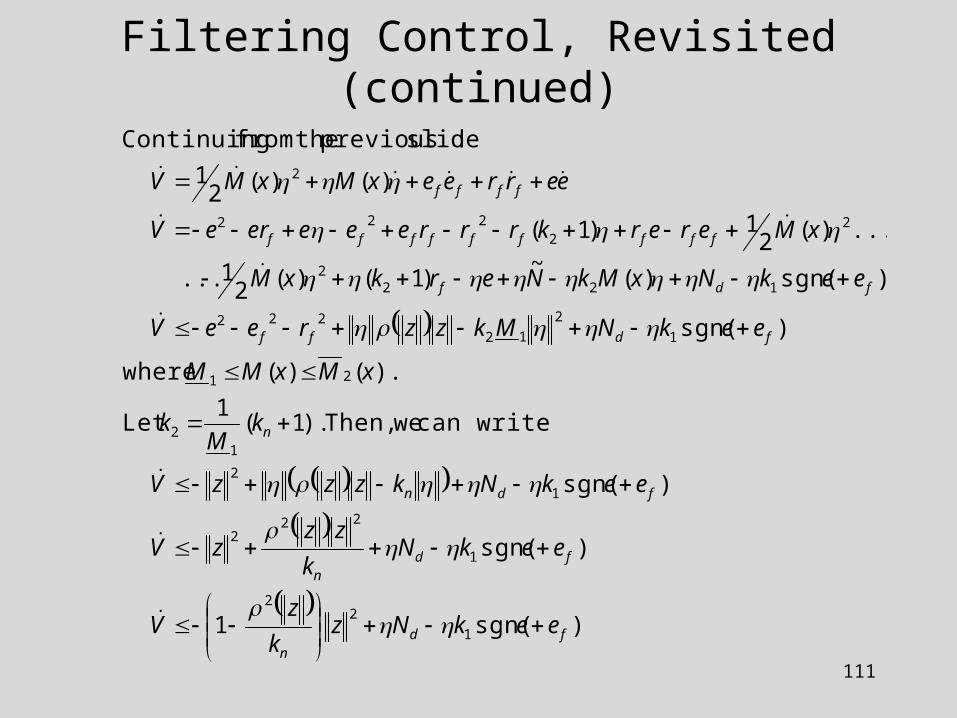
Filtering Control, Revisited (continued)
)sgn(1
)sgn(
)sgn(
can write weThen, ).1(1
Let
).()( where
)sgn(
)sgn()(~
)1()(21...
...)(21)1(
)()(21
:slide previous thefrom Continuing
1
22
1
222
1
2
12
21
1
2
12222
1222
22
222
2
fdn
fdn
fdn
n
fdff
fdf
fffffffff
ffff
eekNzk
zV
eekNk
zzzV
eekNkzzzV
kM
k
xMxMM
eekNMkzzreeV
eekNxMkNerkxM
xMererkrrreeeereV
eerreexMxMV
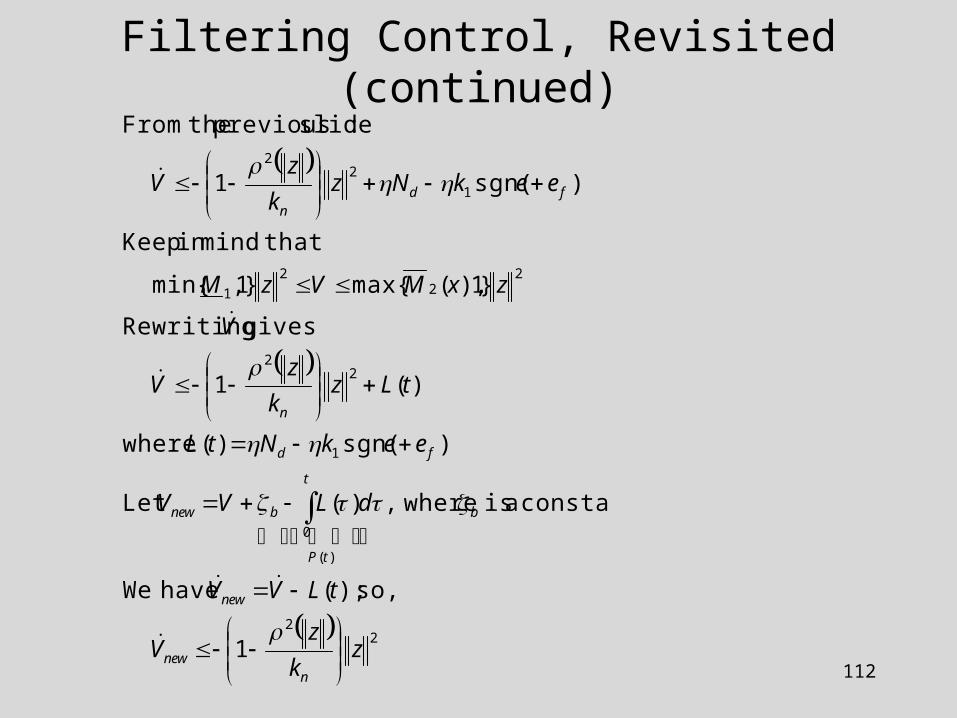
112
22
)(
0
1
22
22
2
1
1
22
1
so, );( have We
constant. a is where,)(Let
)sgn()( where
)(1
gives Rewriting
}1),(max{}1,min{
thatmindin Keep
)sgn(1
:slide previous theFrom
zk
zV
tLVV
dLVV
eekNtL
tLzk
zV
V
zxMVzM
eekNzk
zV
nnew
new
b
tP
t
bnew
fd
n
fdn
Filtering Control, Revisited (continued)

113
Filtering Control, Revisited (continued)
ykzV
zkzV
PzyyM
VyM
tNtetek
NNkP
dkNtP
deekNeeeetP
nnew
nnew
TTnew
dib
dd
t
db
t
t
fdffb
22
22
222
1
0001
1
0
1
0)(
1
for
for
saycan then We
where,}1,2
max{ }1,{2
min
:proof thecomplete tohave weNow,
)()()(Let
if 0 that results previous from know We
done! is Work before. thisdone ve We' )sgn()()(
)sgn()()(
have We
21
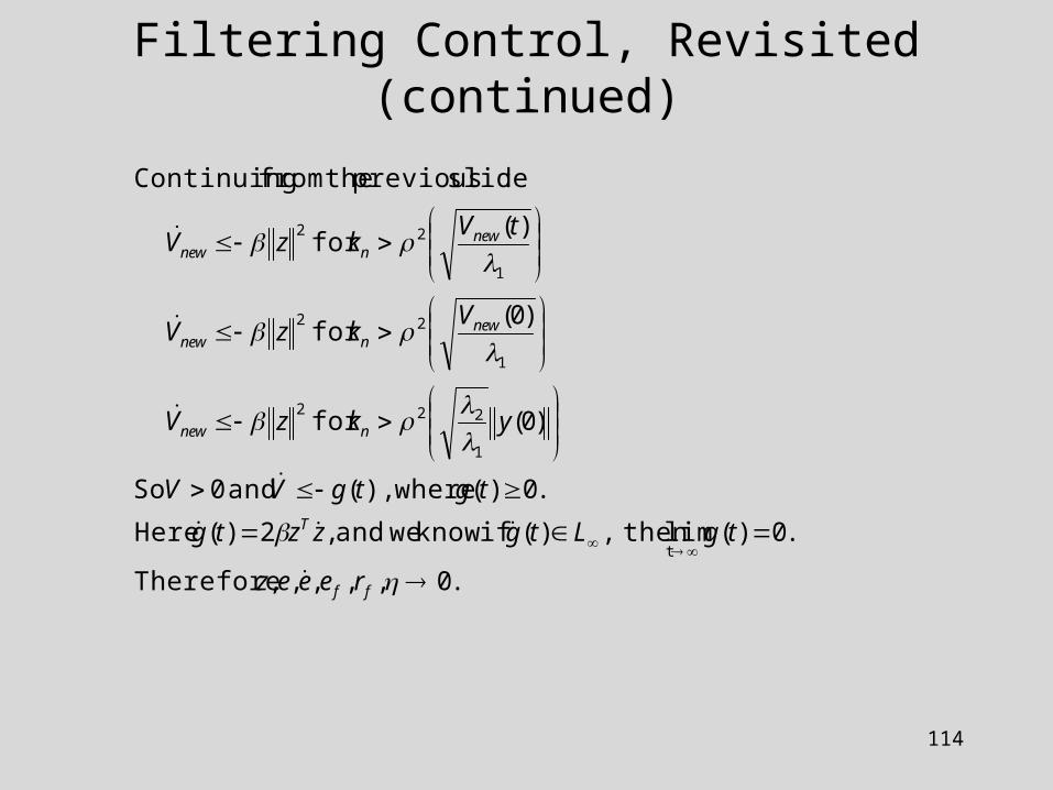
114
Filtering Control, Revisited (continued)
.0,,,,, Therefore
.0)(lim then ,)( if know weand ,2)( Here
.0)( where),( and 0 So
)0(for
)0(for
)(for
:slide previous thefrom Continuing
t
1
222
1
22
1
22
ff
T
nnew
newnnew
newnnew
reeez
tgLtgzztg
tgtgVV
ykzV
VkzV
tVkzV
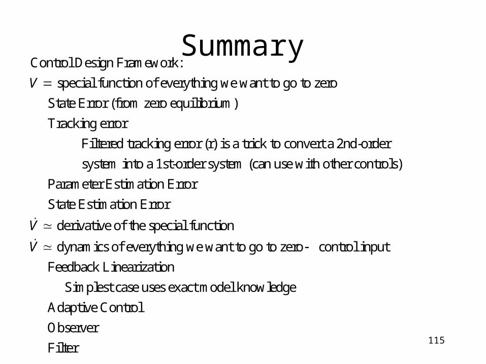
Summary
115
Control Design Framework:
special function of everything we want to go to zero
State Error (from zero equilibrium)
Tracking error
Filtered tracking error (r) is a trick to conv
V
ert a 2nd-order
system into a 1st-order system (can use with other controls)
Parameter Estimation Error
State Estimation Error
derivative of the special function
dynamics
V
V
of everything we want to go to zero control input
Feedback Linearization
Simplest case uses exact model knowledge
Adaptive Control
Observer
Filter

Summary
116
System: ( )
Let the tracking error, , be defined as
( )
1) Control Objective-make ( is a desired trajectory), assuming , .
2) Hidden Control Object
d d d
d d d d
x f x u
e
e x x e x x e x f x u
x x x x x L
ive-keep everything bounded (ie., , , ).
Design a controller based on the tracking error dynamics.
Note that if constant equilibrium point and 0 then
( ), the basicd
x x u L
x u
e x f x
Lyapunov stability analysis tools (Chapter 3) can be used.

Homework A.1
2. Design a contoller for the following system so that tracks cos( ).
where is an unknown constant. Simulate system for 1 plot the state, control, and
and the parameter estimates.
dq q t
q aq u
a a
1. Design a controller for the following system so that tracks cos( ).
where is an constant. Simulate system for 1 plot the state and control.
dq q t
q aq u
a a
Known structure but unknown parameters -> adaptive
Known structure and known parameters -> exact model knowledge control
Partially known structure (unknown component) -> robust
2
3. Design a robust controller for the following system so that tracks cos( ).
where is an unknown constant but you do know <a then < a q +1
Simulate system for 1 and a 3 plot the stat
dq q t
q aq u
a a a q
a
1 2 3e and control comparing , , controllers.
4. Design a learning control for the following system so that tracks cos( ).
where is an unknown constant. Simulate system for 1. Plot t
R R R
d
V V V
q q tq aq u
a a
he state ( ), tracking error,
and control signal ( ).
q t
u t Partially known structure (unknown component), repetitive task -> learning
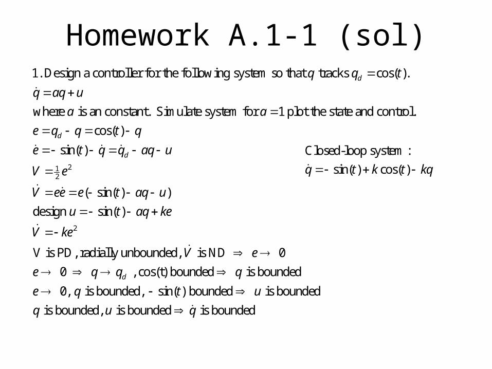
Homework A.1-1 (sol)
12
1. Design a controller for the following system so that tracks cos( ).
where is an constant. Simulate system for 1 plot the state and control.
cos( )
sin( )
d
d
d
q q t
q aq u
a a
e q q t q
e t q q aq u
V e
2
2
( sin( ) )
design sin( )
V is PD, radially unbounded, is ND 0
0 , cos(t) bounded is bounded
0, is bounded, sin( ) bounded is bounded
is bounded,
d
V ee e t aq u
u t aq ke
V ke
V e
e q q q
e q t u
q
is bounded is boundedu q
Closed-loop system :
sin( ) cos( )q t k t kq
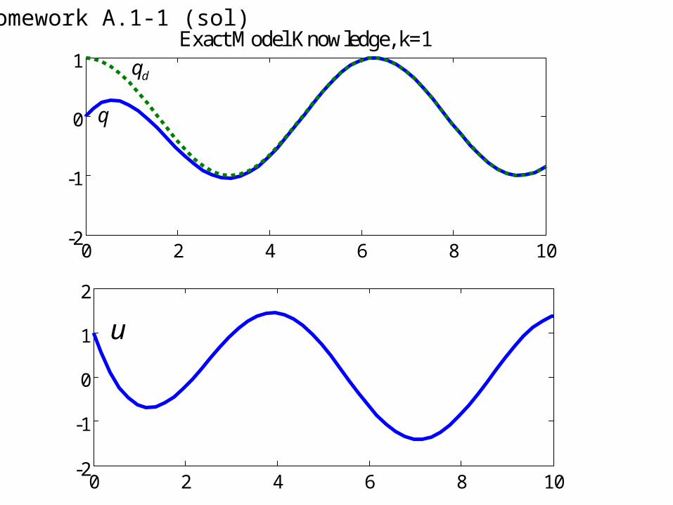
0 2 4 6 8 10-2
-1
0
1
0 2 4 6 8 10-2
-1
0
1
2
dq
q
Exact Model Knowledge, k=1
u
Homework A.1-1 (sol)
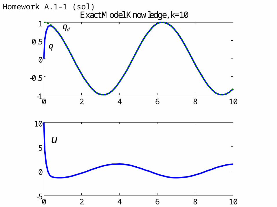
0 2 4 6 8 10-1
-0.5
0
0.5
1
0 2 4 6 8 10-5
0
5
10
Exact Model Knowledge, k=10
dq
q
u
Homework A.1-1 (sol)
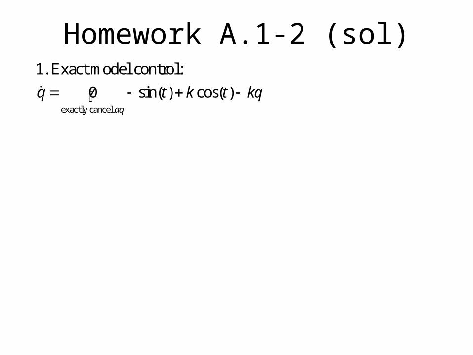
Homework A.1-2 (sol)
exactly cancel
1. Exact model control:
0 sin( ) cos( )aq
q t k t kq
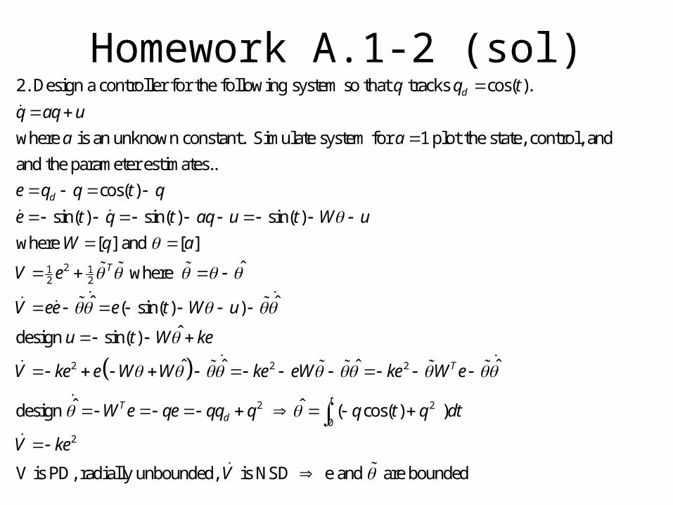
Homework A.1-2 (sol)2. Design a controller for the following system so that tracks cos( ).
where is an unknown constant. Simulate system for 1 plot the state, control, and
and the parameter estimates..
d
d
q q t
q aq u
a a
e q
21 12 2
2 2 2
cos( )
sin( ) sin( ) sin( )
where [ ] and [ ]
ˆ where
ˆ ˆ( sin( ) )
ˆdesign sin( )
ˆ ˆ ˆ
T
q t q
e t q t aq u t W u
W q a
V e
V ee e t W u
u t W ke
V ke e W W ke eW ke
2 2
0
2
ˆ
ˆ ˆdesign ( cos( ) )
V is PD, radially unbounded, is NSD e and are bounded
T
tTd
W e
W e qe qq q q t q dt
V ke
V
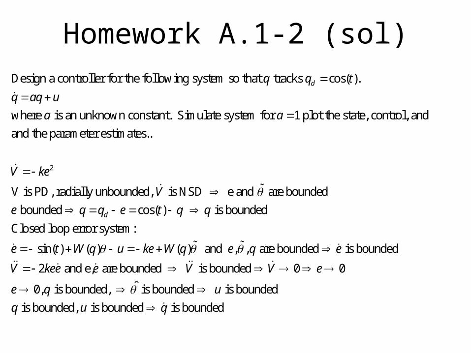
Homework A.1-2 (sol)
2
Design a controller for the following system so that tracks cos( ).
where is an unknown constant. Simulate system for 1 plot the state, control, and
and the parameter estimates..
dq q t
q aq u
a a
V ke
V is PD, radially unbounded, is NSD e and are bounded
bounded cos( ) is bounded
Closed loop error system:
sin( ) ( ) ( ) and , , are bounded is bounded
2
d
V
e q q e t q q
e t W q u ke W q e q e
V
and e, are bounded is bounded 0 0
ˆ0, is bounded, is bounded is bounded
is bounded, is bounded is bounded
kee e V V e
e q u
q u q
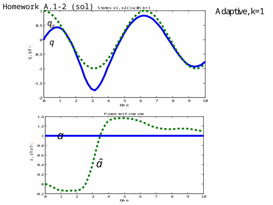
0 1 2 3 4 5 6 7 8 9 10-0.2
0
0.2
0.4
0.6
0.8
1
1.2
1.4
time
a,
ahat-
:
Paremter Estimate
0 1 2 3 4 5 6 7 8 9 10-2
-1.5
-1
-0.5
0
0.5
1
time
q,
qd-:
States x1, x2(:) with k=1
a
a
dq
q
Homework A.1-2 (sol)Adaptive, k=1
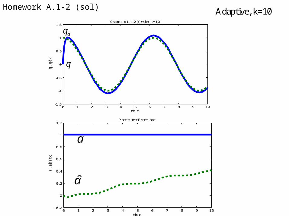
0 1 2 3 4 5 6 7 8 9 10-1.5
-1
-0.5
0
0.5
1
1.5
time
q,
qd-:
States x1, x2(:) with k=10
0 1 2 3 4 5 6 7 8 9 10-0.2
0
0.2
0.4
0.6
0.8
1
1.2
time
a,
ahat-
:
Paremter Estimate
a
a
Adaptive, k=10
dq
q
Homework A.1-2 (sol)
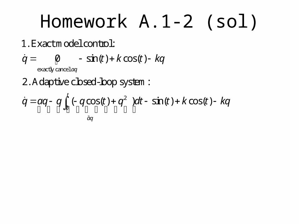
Homework A.1-2 (sol)
exactly cancel
2
0
1. Exact model control:
0 sin( ) cos( )
2. Adaptive closed-loop system:
( cos( ) ) sin( ) cos( )
aq
t
aq
q t k t kq
q aq q q t q dt t k t kq
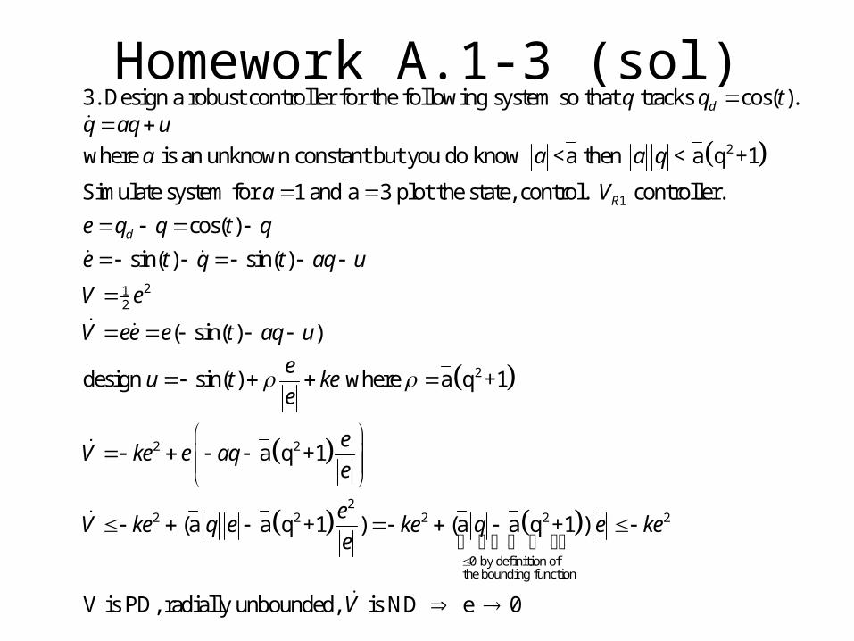
Homework A.1-3 (sol)
2
3. Design a robust controller for the following system so that tracks cos( ).
where is an unknown constant but you do know <a then < a q +1
Simulate system for 1 and a 3 plot the stat
dq q tq aq u
a a a q
a
1
212
2
2 2
22 2 2 2
e, control. controller.
cos( )
sin( ) sin( )
( sin( ) )
design sin( ) where a q +1
a q +1
(a a q +1 ) (a a q +1
R
d
V
e q q t q
e t q t aq u
V e
V ee e t aq u
eu t ke
e
eV ke e aq
e
eV ke q e ke q
e
2
0 by definition of the bounding function
)
V is PD, radially unbounded, is ND e 0
e ke
V
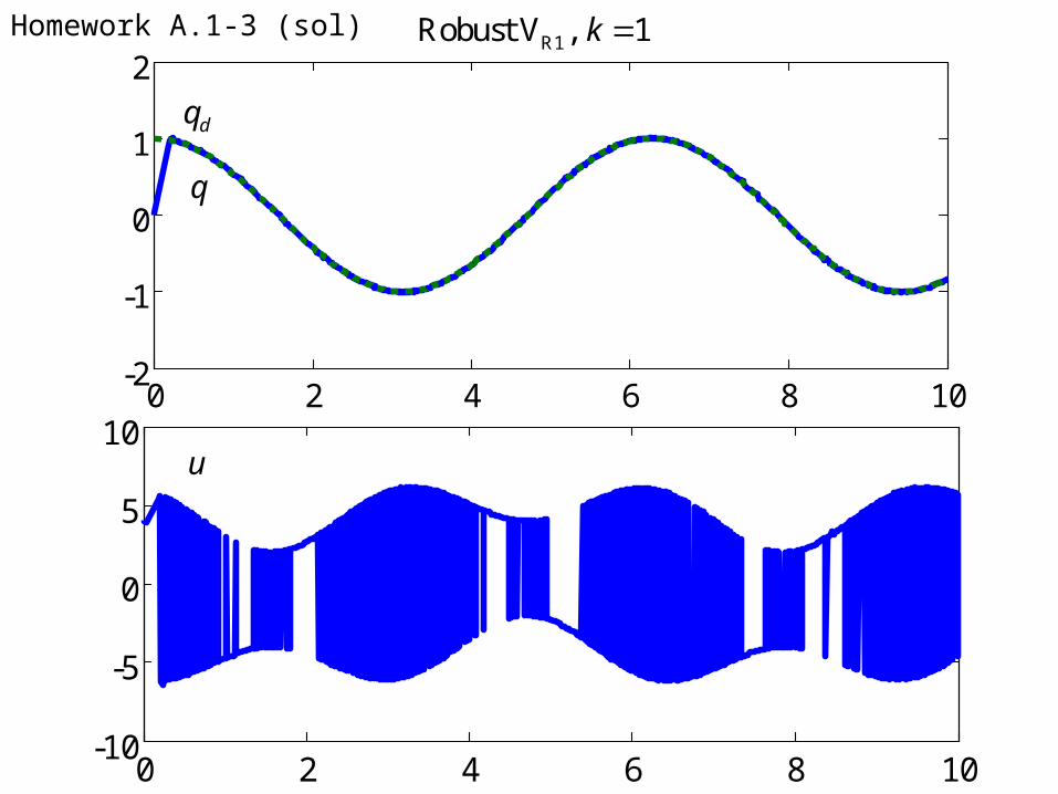
k=1
0 2 4 6 8 10-10
-5
0
5
100 2 4 6 8 10
-2
-1
0
1
2R1Robust V , 1k
dq
q
u
Homework A.1-3 (sol)
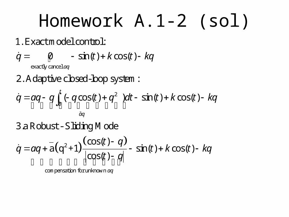
Homework A.1-2 (sol)
exactly cancel
2
0
2
1. Exact model control:
0 sin( ) cos( )
2. Adaptive closed-loop system:
( cos( ) ) sin( ) cos( )
3.a Robust - Sliding Mode
cos( )a q +1
cos(
aq
t
aq
q t k t kq
q aq q q t q dt t k t kq
t qq aq
t
compensation for unknown
sin( ) cos( ))
aq
t k t kqq
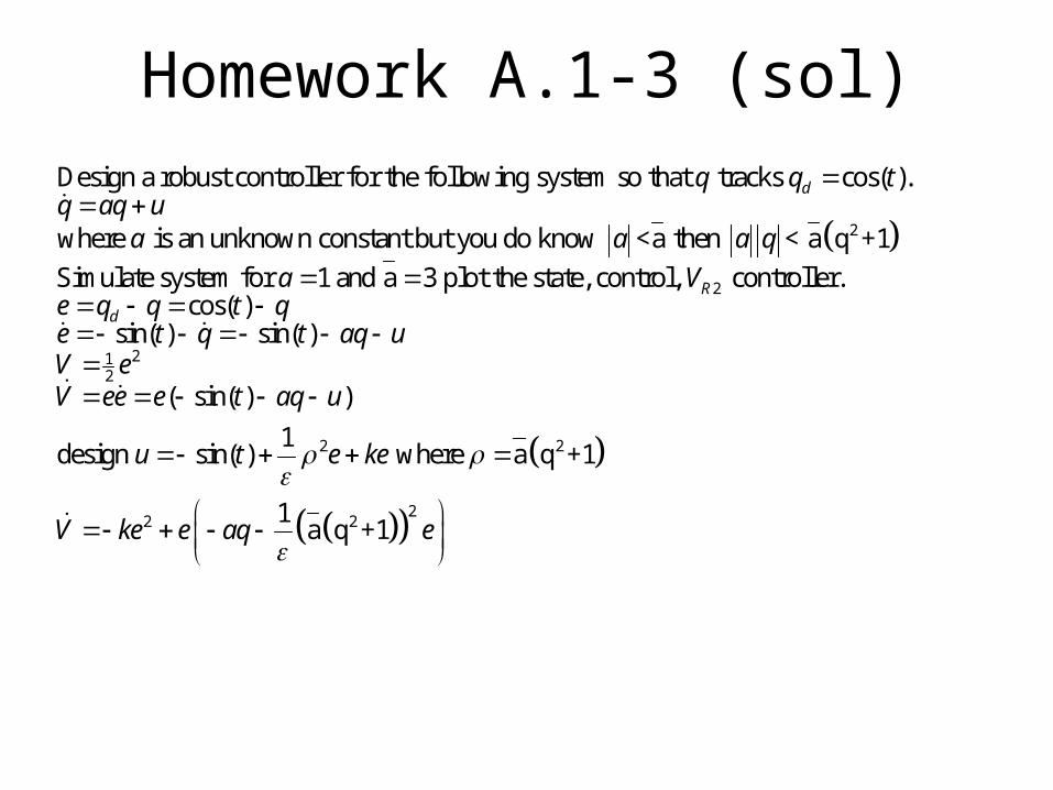
Homework A.1-3 (sol)
2
Design a robust controller for the following system so that tracks cos( ).
where is an unknown constant but you do know <a then < a q +1
Simulate system for 1 and a 3 plot the state,
dq q tq aq u
a a a q
a
2
212
2 2
22 2
control, controller.cos( )
sin( ) sin( )
( sin( ) )
1design sin( ) where a q +1
1a q +1
R
d
Ve q q t qe t q t aq uV eV ee e t aq u
u t e ke
V ke e aq e
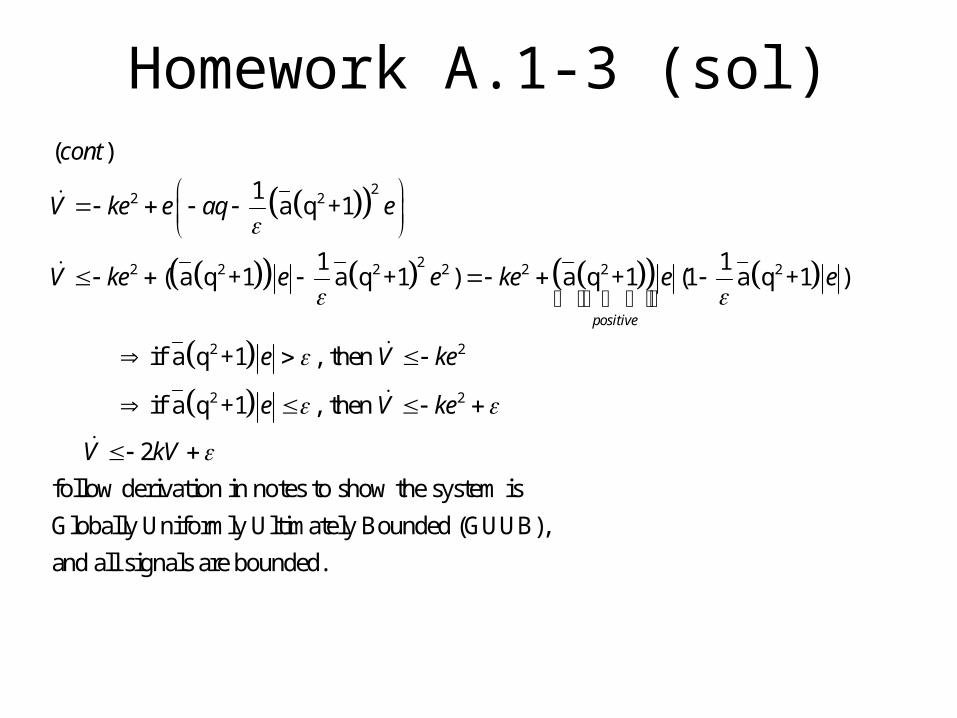
Homework A.1-3 (sol)
22 2
22 2 2 2 2 2 2
2 2
2 2
( )
1a q +1
1 1( a q +1 a q +1 ) a q +1 (1 a q +1 )
if a q +1 , then
if a q +1 , then
2
follow deriv
positive
cont
V ke e aq e
V ke e e ke e e
e V ke
e V ke
V kV
ation in notes to show the system is
Globally Uniformly Ultimately Bounded (GUUB),
and all signals are bounded.
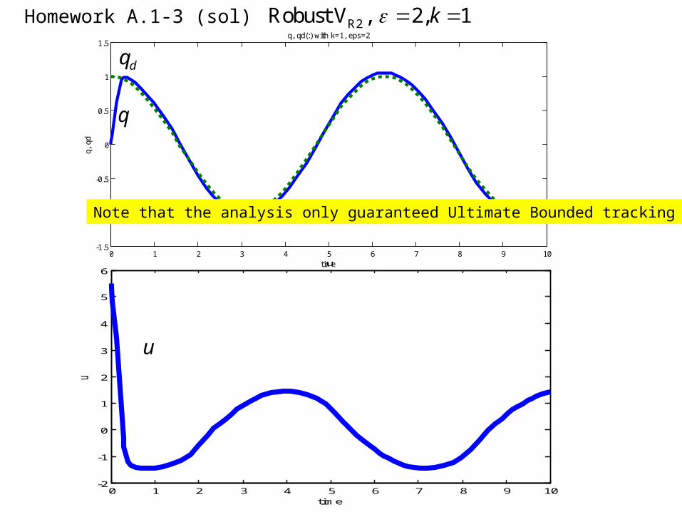
0 1 2 3 4 5 6 7 8 9 10-1.5
-1
-0.5
0
0.5
1
1.5
time
q, q
d
q, qd(:) with k=1, eps=2
0 1 2 3 4 5 6 7 8 9 10-2
-1
0
1
2
3
4
5
6
time
u
u
R2Robust V , 2, 1k
dq
q
u
Note that the analysis only guaranteed Ultimate Bounded tracking error.
Homework A.1-3 (sol)
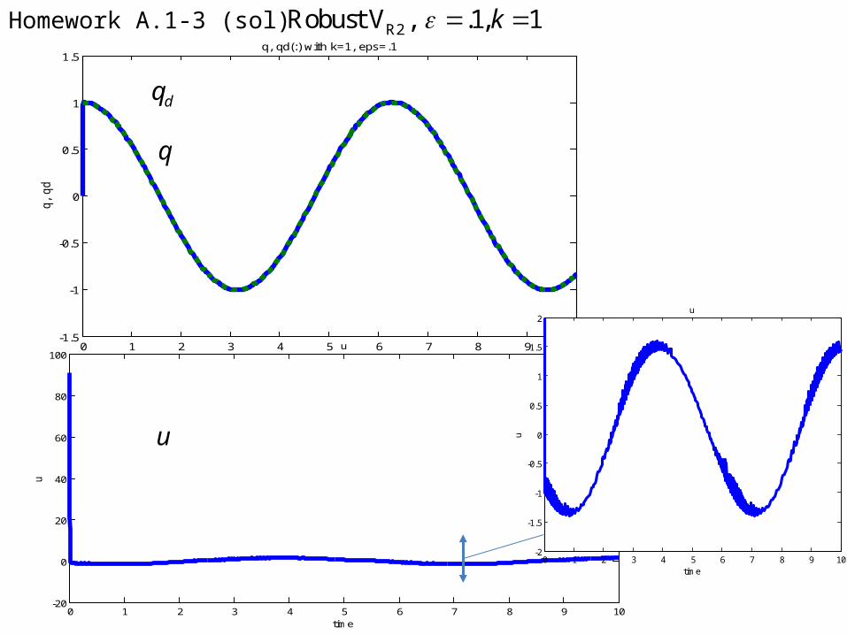
0 1 2 3 4 5 6 7 8 9 10-1.5
-1
-0.5
0
0.5
1
1.5
time
q,
qd
q, qd(:) with k=1, eps=.1
0 1 2 3 4 5 6 7 8 9 10-20
0
20
40
60
80
100
time
u
u
R2Robust V , .1, 1k
dq
q
u
Homework A.1-3 (sol)
0 1 2 3 4 5 6 7 8 9 10-2
-1.5
-1
-0.5
0
0.5
1
1.5
2
time
u
u
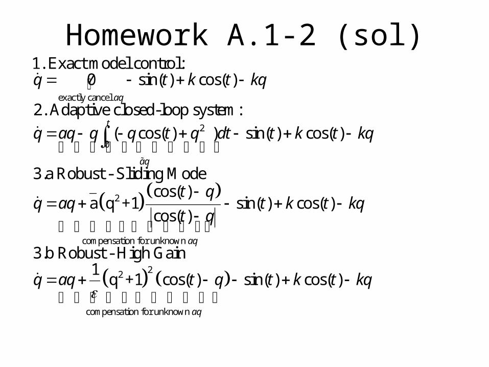
Homework A.1-2 (sol)
exactly cancel
2
0
2
1. Exact model control:0 sin( ) cos( )
2. Adaptive closed-loop system:
( cos( ) ) sin( ) cos( )
3.a Robust - Sliding Modecos( )
a q +1cos(
aq
t
aq
q t k t kq
q aq q q t q dt t k t kq
t qq aq
t
compensation for unknown
22
compensation for unknown
sin( ) cos( ))
3.b Robust - High Gain1
q +1 cos( ) sin( ) cos( )
aq
aq
t k t kqq
q aq t q t k t kq

Homework A.1-3 (sol)
2
Design a robust controller for the following system so that tracks cos( ).
where is an unknown constant but you do know <a then < a q +1
Simulate system for 1 and a 3 plot the state,
dq q tq aq u
a a a q
a
3
212
22
2 22 2 2
2 2 2
2 2
control, controller.cos( ) ; sin( ) sin( )
( sin( ) )
design sin( ) where a q +1
a q +1 a q +1a q +1
a q +1 a q +1
R
d
Ve q q t q e t q t aq uV eV ee e t aq u
eu t ke
e
e eV ke e aq ke e
e
2 222 2 2 2 2
2 2
2 2
1
2
a q +1 a q +1 a q +1 a q +1
a q +1 a q +1
follow derivation from notes.
e
e e e eV ke ke
e e
V ke
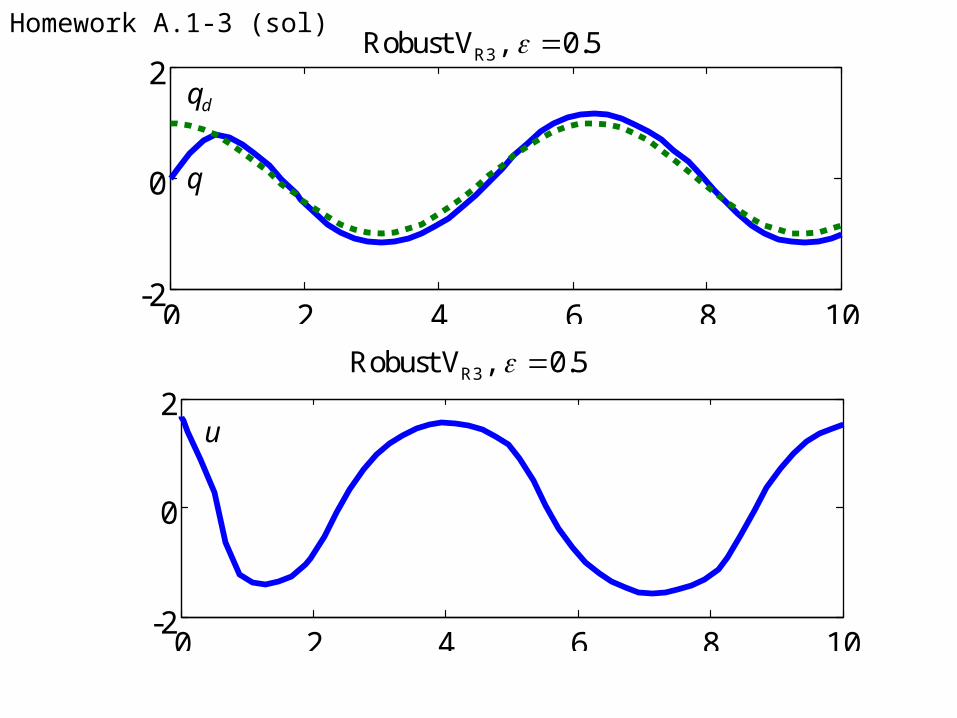
0 2 4 6 8 10-2
0
2
0 2 4 6 8 10-2
0
2
R3Robust V , 0.5
dq
q
u
R3Robust V , 0.5
Homework A.1-3 (sol)
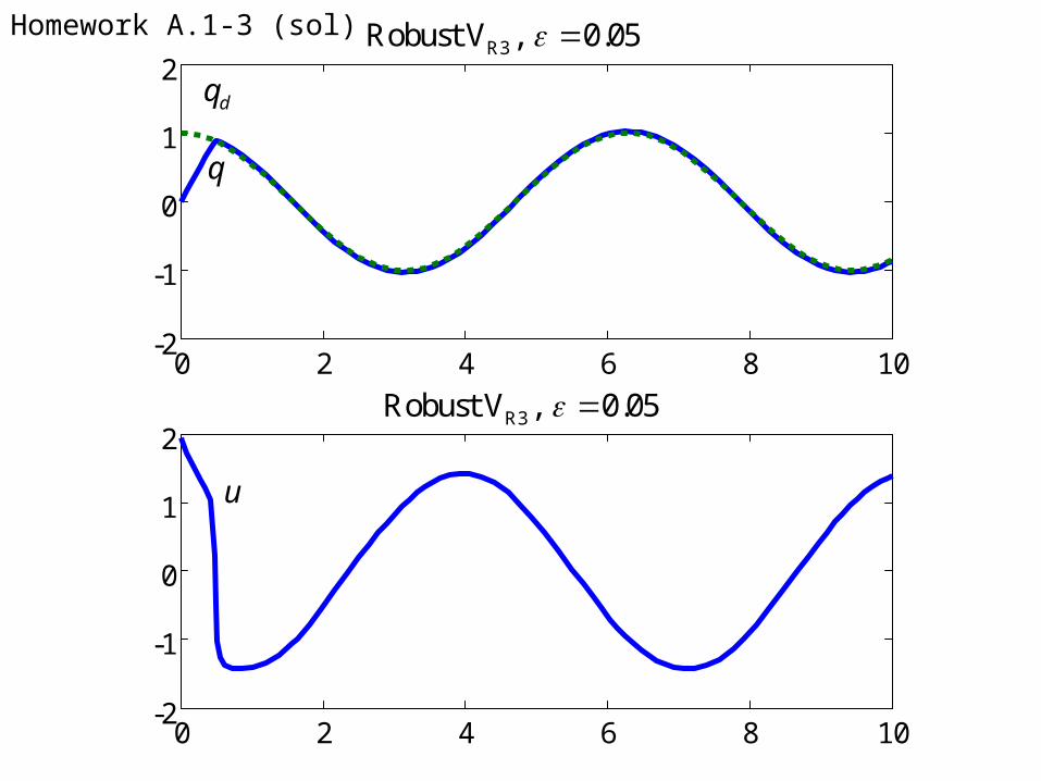
0 2 4 6 8 10-2
-1
0
1
2
0 2 4 6 8 10-2
-1
0
1
2
R3Robust V , 0.05
dq
q
R3Robust V , 0.05
u
Homework A.1-3 (sol)
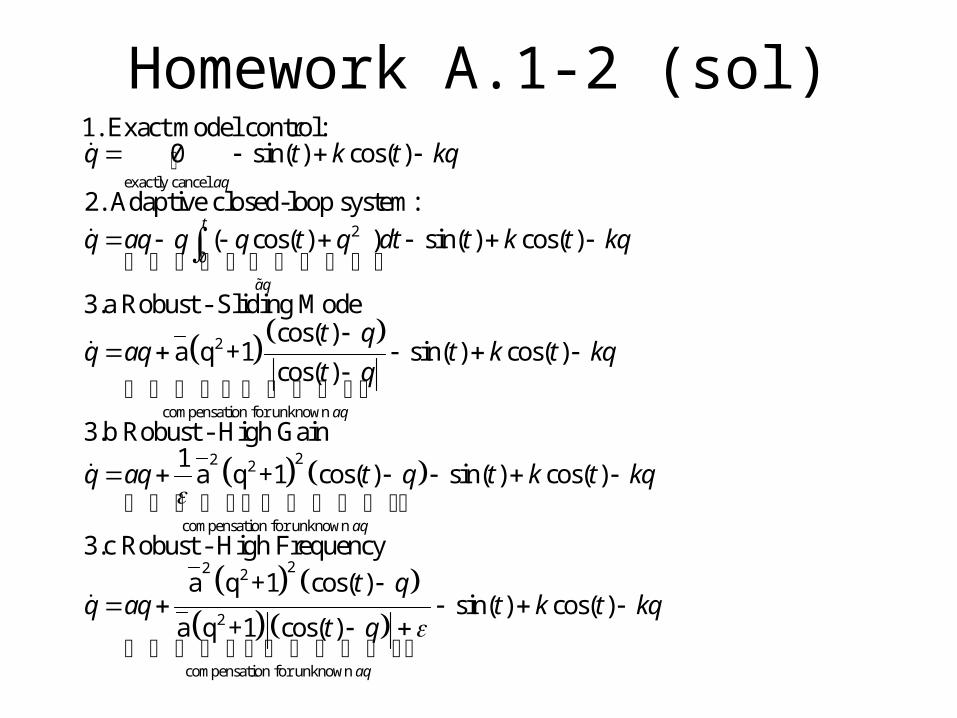
Homework A.1-2 (sol)
exactly cancel
2
0
2
1. Exact model control:0 sin( ) cos( )
2. Adaptive closed-loop system:
( cos( ) ) sin( ) cos( )
3.a Robust - Sliding Modecos( )
a q +1cos(
aq
t
aq
q t k t kq
q aq q q t q dt t k t kq
t qq aq
t
compensation for unknown
22 2
compensation for unknown
2 2
sin( ) cos( ))
3.b Robust - High Gain1
a q +1 cos( ) sin( ) cos( )
3.c Robust - High Frequency
a q +
aq
aq
t k t kqq
q aq t q t k t kq
q aq
2
2
compensation for unknown
1 cos( )sin( ) cos( )
a q +1 cos( )
aq
t qt k t kq
t q
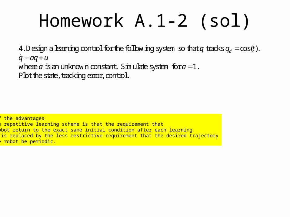
4. Design a learning control for the following system so that tracks cos( ).
where is an unknown constant. Simulate system for 1. Plot the state, tracking error, control.
dq q tq aq u
a a
Homework A.1-2 (sol)
One of the advantagesof the repetitive learning scheme is that the requirement thatthe robot return to the exact same initial condition after each learningtrial is replaced by the less restrictive requirement that the desired trajectoryof the robot be periodic.
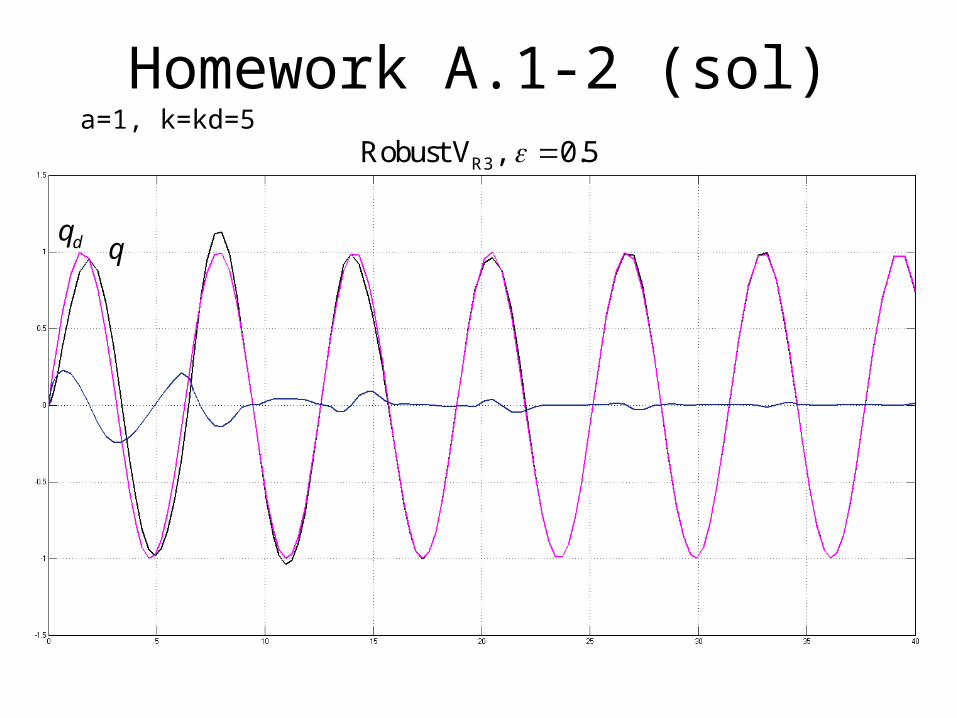
Homework A.1-2 (sol)a=1, k=kd=5
R3Robust V , 0.5
dqq
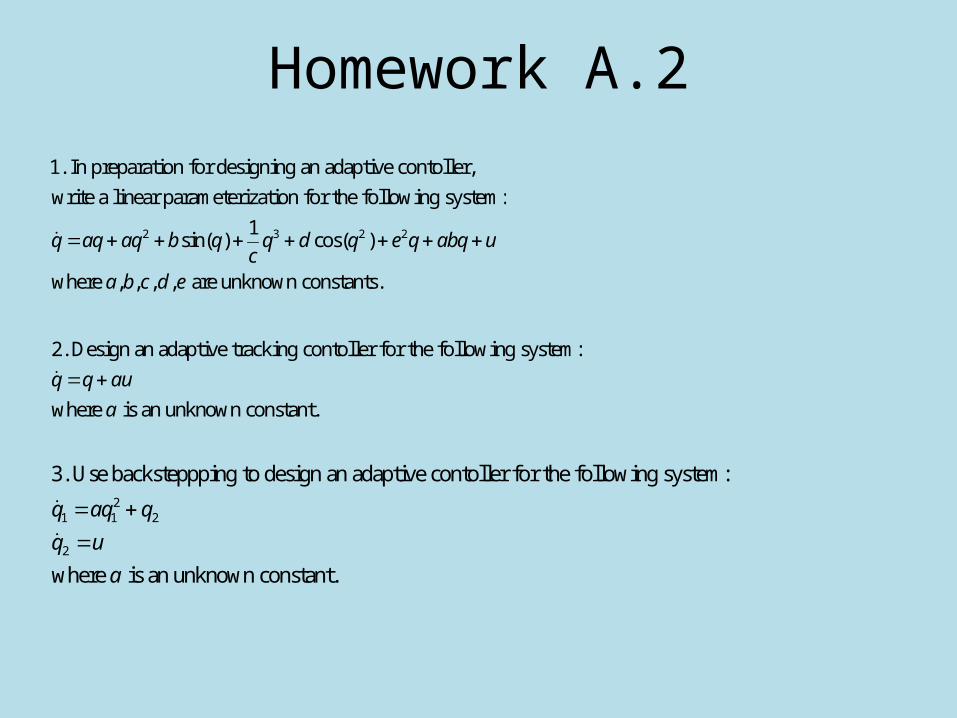
Homework A.2
2. Design an adaptive tracking contoller for the following system:
where is an unknown constant.
q q au
a
21 1 2
2
3. Use backsteppping to design an adaptive contoller for the following system:
where is an unknown constant.
q aq q
q u
a
2 3 2 2
1. In preparation for designing an adaptive contoller,
write a linear parameterization for the following system:
1sin( ) cos( )
where , , , , are unknown constants.
q aq aq b q q d q e q abq uc
a b c d e
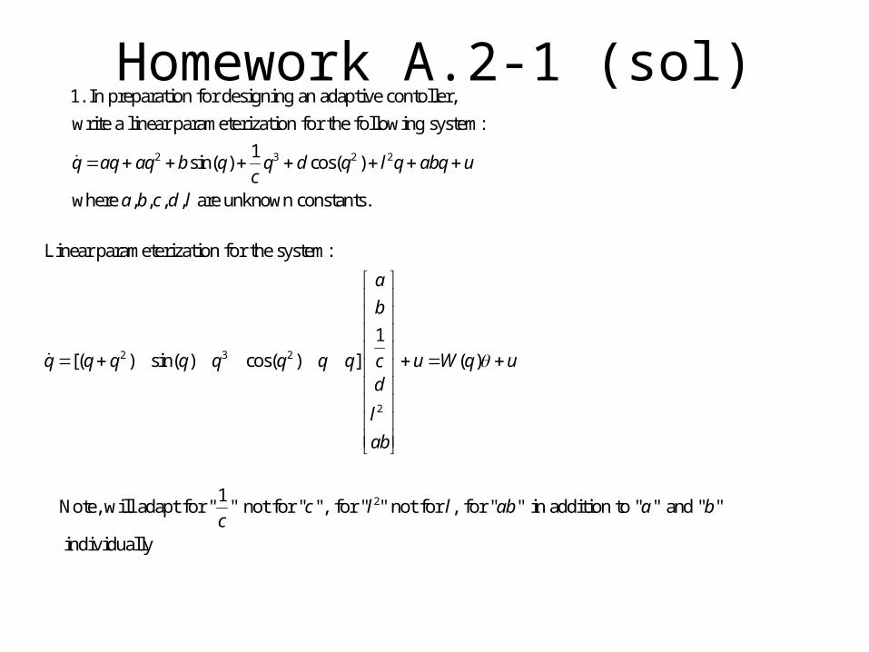
Homework A.2-1 (sol)
2 3 2 2
1. In preparation for designing an adaptive contoller,
write a linear parameterization for the following system:
1sin( ) cos( )
where , , , , are unknown constants.
q aq aq b q q d q l q abq uc
a b c d l
2 3 2
2
Linear parameterization for the system:
1
[( ) sin( ) cos( ) ] ( )
a
b
q q q q q q q q u W q ucd
l
ab
21Note, will adapt for " " not for " ", for " " not for , for " " in addition to " " and " "
individually
c l l ab a bc

Homework A.2-2 (sol)2. Design an adaptive tracking contoller for the following system:
where is an unknown constant.
Looks harmless but note that anything we put in will get multiplied by " ".
1Can't include i
q q au
a
u a
a
n since is unknown.u a
1 1
2 12
1 1 1 12 2 2 2
Rewrite as:1 1
1 1 1 1where [ ] and
1 ˆ where 21 1 1ˆ ˆ ˆ
substitue -dynamics:
d d d
T
T T T T
q q u W ua a
e q q q W u W u W q qa a a a
V ea
V ee ee eea a a
e
1
1
2 2 21 1 1
12
ˆ( )ˆdesign
ˆ ˆ ˆ
ˆdesign [ ]
V is PD, radially unbounded, is NSD e and are bounded
T T
Td
V e W u
u W ke
V ke eW ke W e ke W e
W e q q eV ke
V
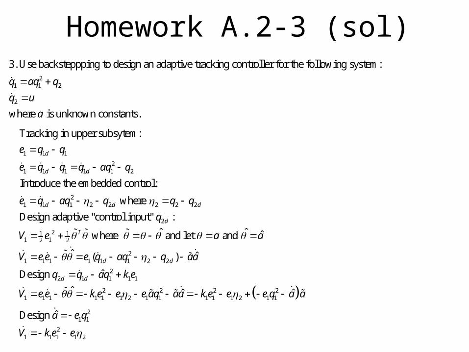
Homework A.2-3 (sol)2
1 1 2
2
3. Use backsteppping to design an adaptive tracking controller for the following system:
where is unknown constants.
q aq q
q u
a
1 1 1
21 1 1 1 1 2
21 1 1 2 2 2 2 2
2
21 11 12 2
Tracking in upper subsytem:
Introduce the embedded control:
where
Design adaptive "control input" :
ˆ where and
d
d d
d d d
d
T
e q q
e q q q aq q
e q aq q q q
q
V e
21 1 1 1 1 1 2 2
22 1 1 1 1
2 2 2 21 1 1 1 1 1 2 1 1 1 1 1 2 1 1
21 1
21 1 1 1 2
ˆ ˆlet and
ˆ ˆ( )
ˆDesign
ˆ ˆ ˆ
ˆDesign
d d
d d
a a
V e e e q aq q aa
q q aq k e
V e e k e e e aq aa k e e e q a a
a e q
V k e e
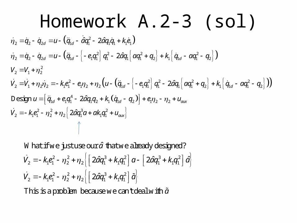
Homework A.2-3 (sol)
22 2 2 1 1 1 1 1 1
2 2 2 22 2 2 1 1 1 1 1 1 2 1 1 1 2
22 1 2
2 2 2 2 22 1 2 2 1 1 1 2 2 1 1 1 1 1 1 2 1 1 1 2
1 1
ˆ ˆ2
ˆ2
ˆ2
Design
d d
d d d
d d
d
q q u q aq aq q k e
q q u q e q q aq aq q k q aq q
V V
V V k e e u q e q q aq aq q k q aq q
u q e q
41 1 2 1 1 2 1 2 2
2 2 3 22 1 1 2 2 1 1 1
ˆ2
ˆ2
d aux
aux
aq q k q q e u
V k e aq a ak q u
2 2 3 2 3 22 1 1 2 2 1 1 1 1 1 1
2 2 3 22 1 1 2 2 1 1 1
ˆWhat if we just use our that we already designed?
ˆ ˆ ˆ2 2
ˆ2
This is a problem because we can't deal with
a
V k e aq k q a aq k q a
V k e aq k q a
a
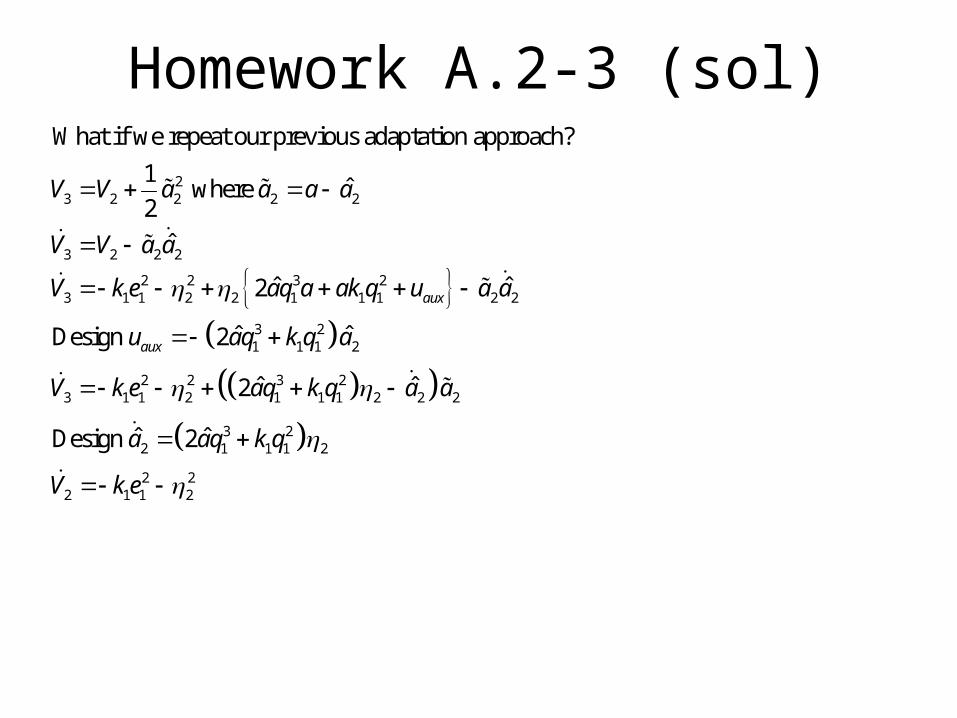
Homework A.2-3 (sol)
23 2 2 2 2
3 2 2 2
2 2 3 23 1 1 2 2 1 1 1 2 2
3 21 1 1 2
2 2 3 23 1 1 2 1 1 1 2 2
What if we repeat our previous adaptation approach?
1ˆ where
2
ˆ
ˆ ˆ2
ˆ ˆDesign 2
ˆ ˆ2
aux
aux
V V a a a a
V V a a
V k e aq a ak q u a a
u aq k q a
V k e aq k q a
2
3 22 1 1 1 2
2 22 1 1 2
ˆ ˆDesign 2
a
a aq k q
V k e
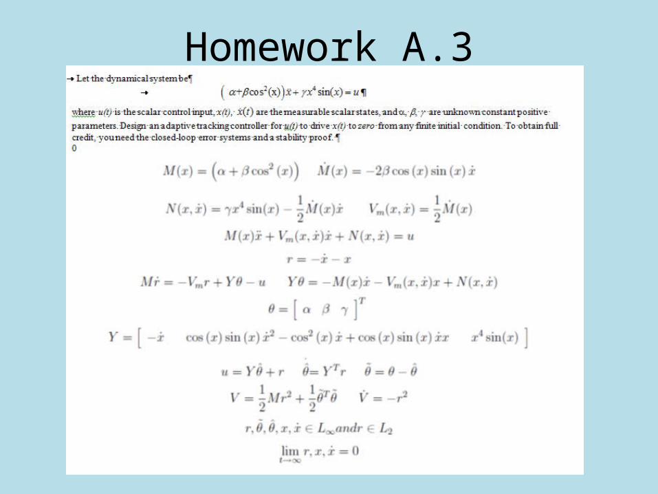
Homework A.3

Homework A.3
2.
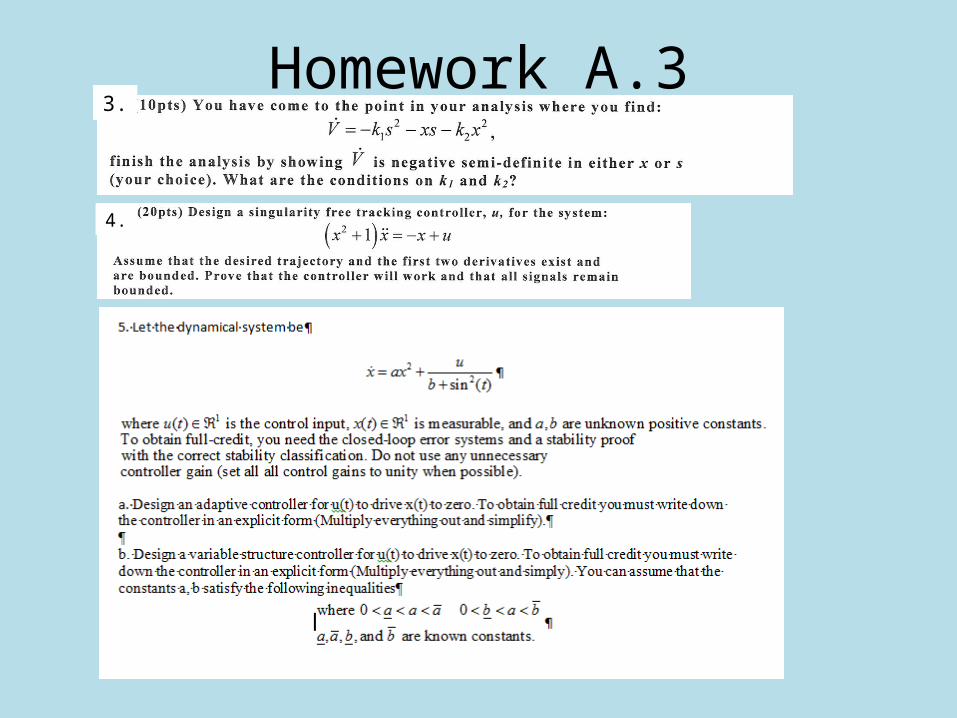
Homework A.33.
4.
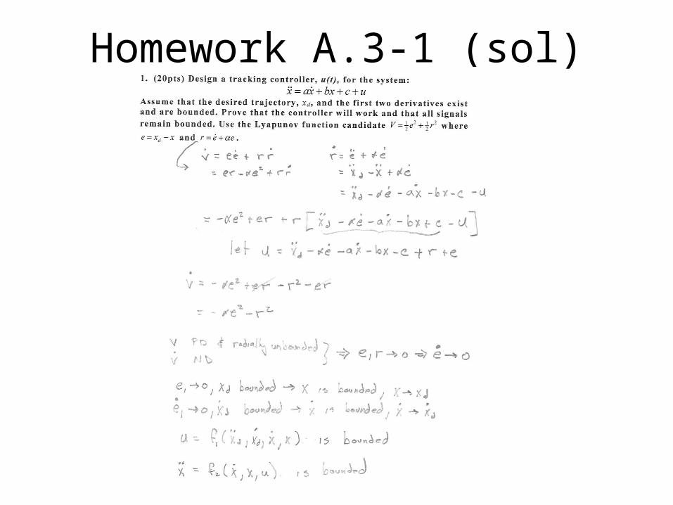
Homework A.3-1 (sol)
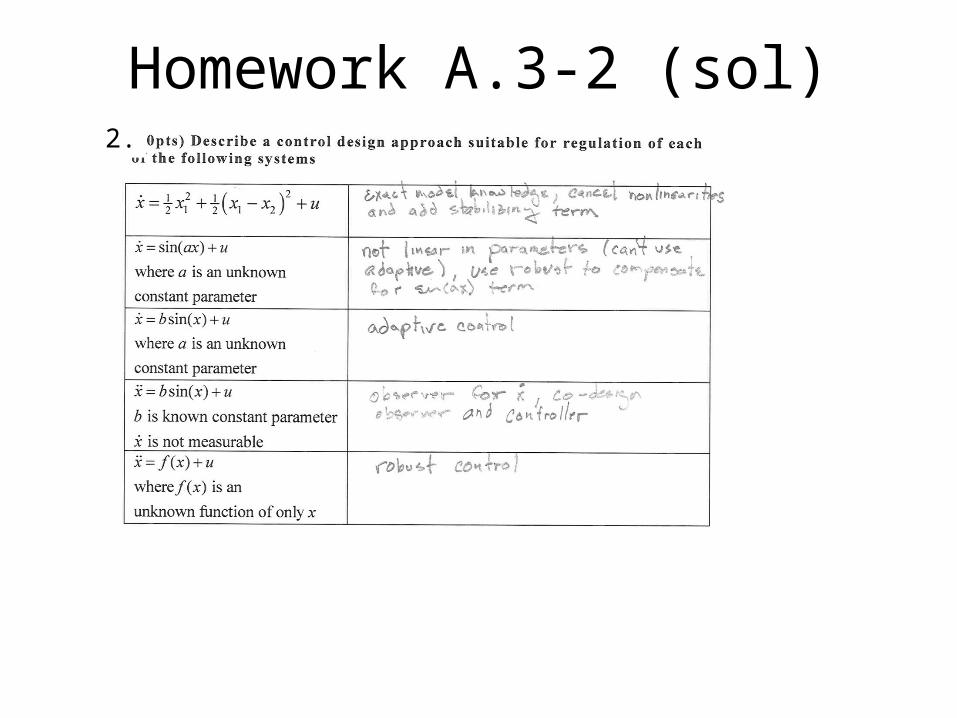
Homework A.3-2 (sol)2.

Homework A.3-3 (sol)3.
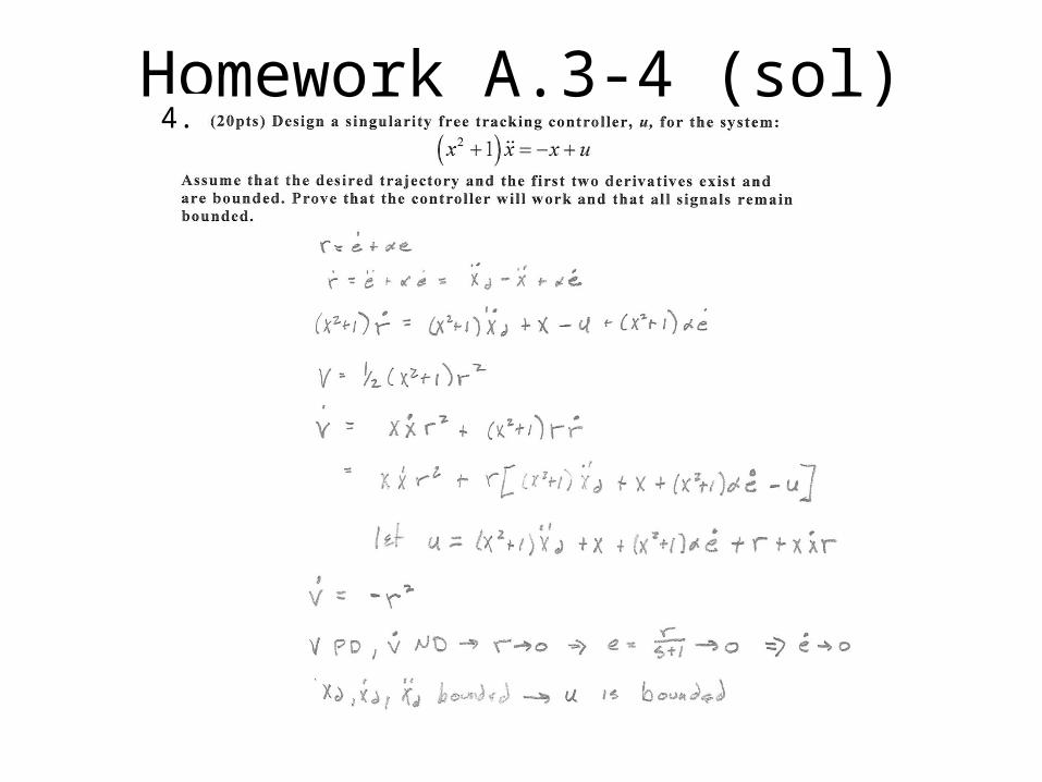
Homework A.3-4 (sol)4.
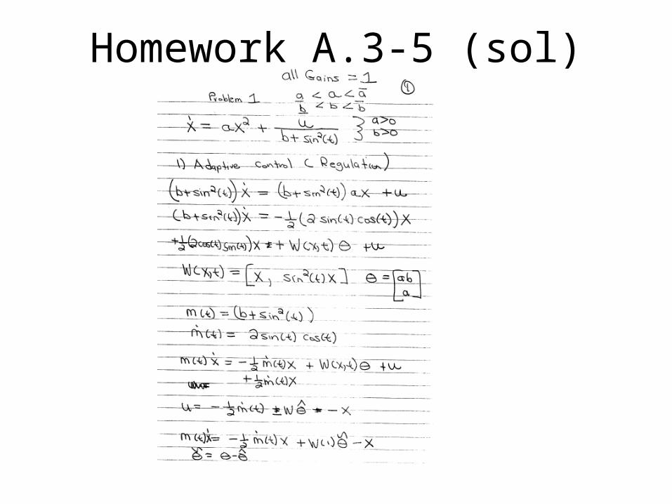
Homework A.3-5 (sol)
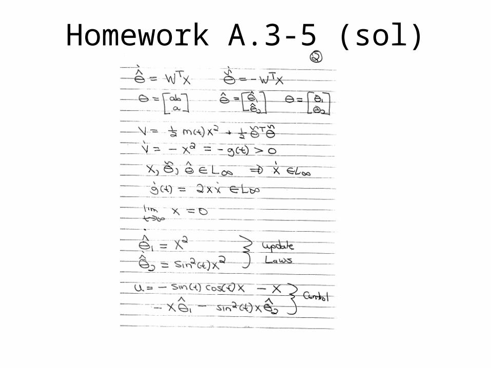
Homework A.3-5 (sol)
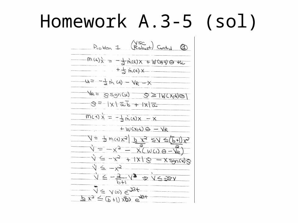
Homework A.3-5 (sol)
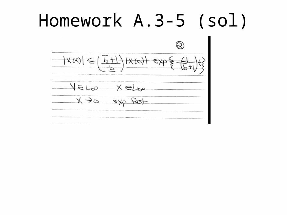
Homework A.3-5 (sol)

Homework A.4
2
1. Design an observer to estimate in the open-loop system:
2cos( )
( is measureable but is not).
x
x x u
x x
2
2. Design an observer to estimate and a tracking controller for x in the system:
2cos( )
( is measureable but is not).
x
x x u
x x
2
3. Design a filter and a tracking controller for x in the system:
2cos( )
( is measureable but is not).
x x u
x x
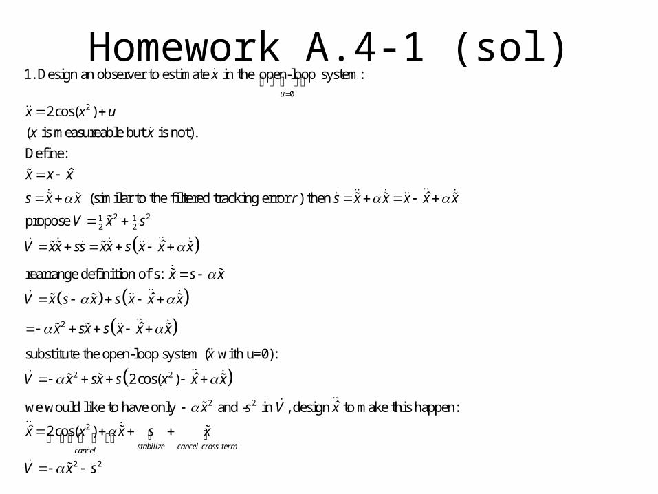
0
2
1. Design an observer to estimate in the open-loop system:
2cos( )
( is measureable but is not).
Define:
ˆ
(similar to the filtered tracking error ) then
u
x
x x u
x x
x x x
s x x r s x
2 21 12 2
2
ˆ
propose
ˆ
rearrange definition of s:
ˆ
ˆ
substitute the open-loop system ( with u=0
x x x x
V x s
V xx ss xx s x x x
x s x
V x s x s x x x
x sx s x x x
x
2 2
2 2
2
2 2
):
ˆ2cos( )
ˆwe would like to have only and - in , design to make this happen:
ˆ 2cos( )stabilize cancel cross termcancel
V x sx s x x x
x s V x
x x x s x
V x s
Homework A.4-1 (sol)
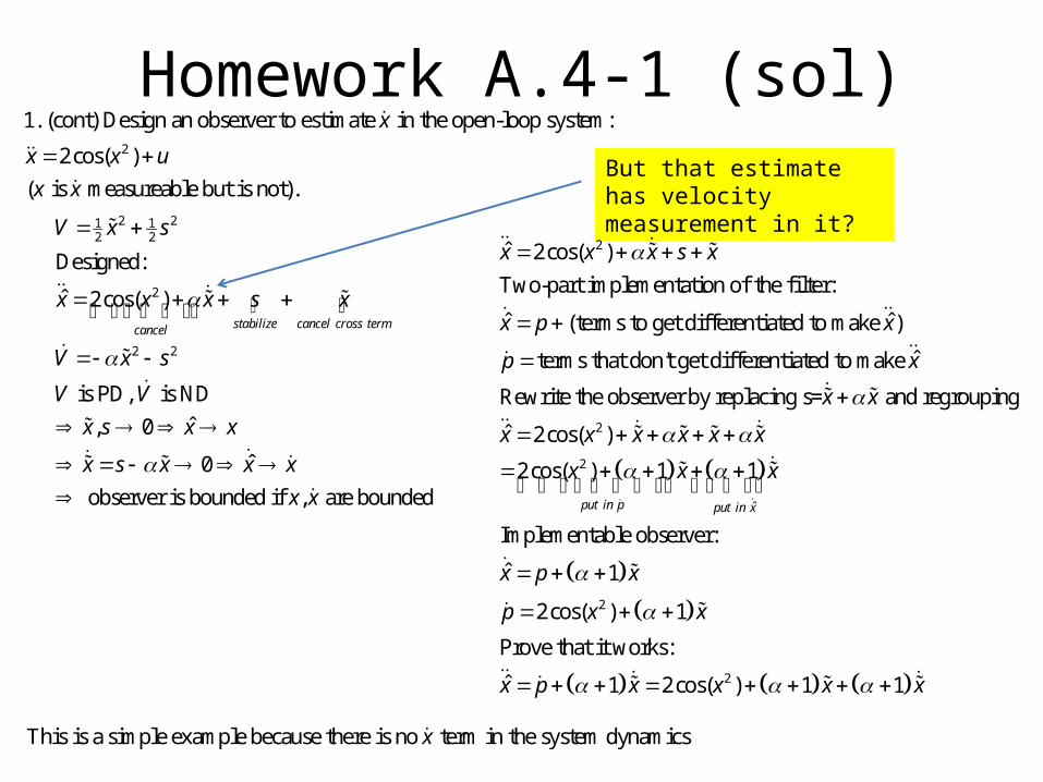
2
1. (cont) Design an observer to estimate in the open-loop system:
2cos( )
( is measureable but is not).
x
x x u
x x
Homework A.4-1 (sol)
2 21 12 2
2
2 2
Designed:
ˆ 2cos( )
is PD, is ND
ˆ, 0
ˆ0
observer is bounded if , are bounded
stabilize cancel cross termcancel
V x s
x x x s x
V x s
V V
x s x x
x s x x x
x x
2ˆ 2cos( )
Two-part implementation of the filter:
ˆ ˆ(terms to get differentiated to make )
ˆterms that don't get differentiated to make
Rewrite the observer by replacing s=
x x x s x
x p x
p x
x
2
2
ˆ
2
2
and regrouping
ˆ 2cos( )
2cos( ) 1 1
Implementable observer:
ˆ 1
2cos( ) 1
Prove that it works:
ˆ 1 2cos( ) 1
put in p put in x
x
x x x x x x
x x x
x p x
p x x
x p x x
1x x
But that estimate has velocity measurement in it?
This is a simple example because there is no term in the system dynamicsx
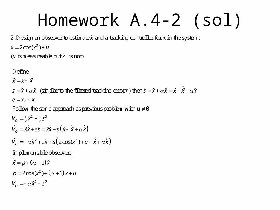
Homework A.4-2 (sol)2
2. Design an observer to estimate and a tracking controller for x in the system:
2cos( )
( is measureable but is not).
x
x x u
x x
2 21 12 2
Define:
ˆ
ˆ (similar to the filtered tracking error ) then
Follow the same approach as previous problem with u 0
ˆ
d
O
O
x x x
s x x r s x x x x x
e x x
V x s
V xx ss xx s x x
2 2
2
2 2
ˆ2cos( )
Implementable observer:
ˆ 1
2cos( ) 1
O
O
x
V x sx s x u x x
x p x
p x x u
V x s
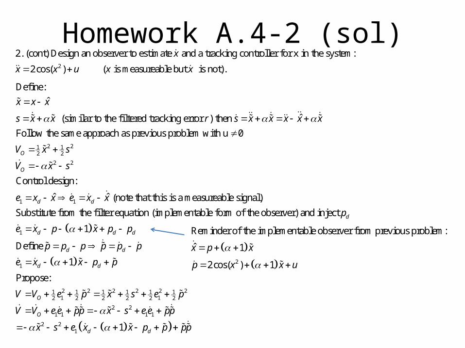
Homework A.4-2 (sol)2
2. (cont) Design an observer to estimate and a tracking controller for x in the system:
2cos( ) ( is measureable but is not).
x
x x u x x
2 21 12 2
2 2
1
Define:
ˆ
ˆ (similar to the filtered tracking error ) then
Follow the same approach as previous problem with u 0
Control design:
ˆ
O
O
d
x x x
s x x r s x x x x x
V x s
V x s
e x x
1
1
1
ˆ (note that this is a measureable signal)
Substitute from the filter equation (implementable form of the observer) and inject
1
Define
1
d
d
d d d
d d
d
e x x
p
e x p x p p
p p p p p p
e x x p
2 2 2 2 2 21 1 1 1 1 11 12 2 2 2 2 2
2 21 1 1 1
2 21
Propose:
1
d
O
O
d d
p
V V e p x s e p
V V e e pp x s e e pp
x s e x x p p pp
2
Reminder of the implementable observer from previous problem:
ˆ 1
2cos( ) 1
x p x
p x x u
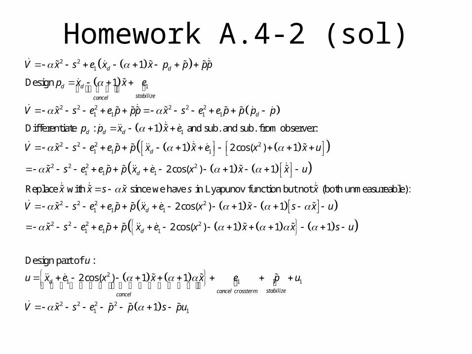
Homework A.4-2 (sol)
2 21
1
2 2 2 2 2 21 1 1 1
1
1
Design 1
Differentiate : 1 and sub. and sub. from observe
d d
d d
stabilizecancel
d
d d d
V x s e x x p p pp
p x x e
V x s e e p pp x s e e p p p p
p p x x e
2 2 2 21 1 1
2 2 2 21 1 1
r:
1 2cos( ) 1
2cos( ) 1 1
Replace with since we have in Lyapunov function but not (b
d
d
V x s e e p p x x e x x u
x s e e p p x e x x x u
x x s x s x
2 2 2 21 1 1
2 2 2 21 1 1
21
oth unmeasureable):
2cos( ) 1 1
2cos( ) 1 1 1
Design part of :
2cos( ) 1 1
d
d
d
cancel
V x s e e p p x e x x s x u
x s e e p p x e x x x s u
u
u x e x x x
1 1
2 2 2 21 11
stabilizecancel crossterm
e p u
V x s e p p s pu
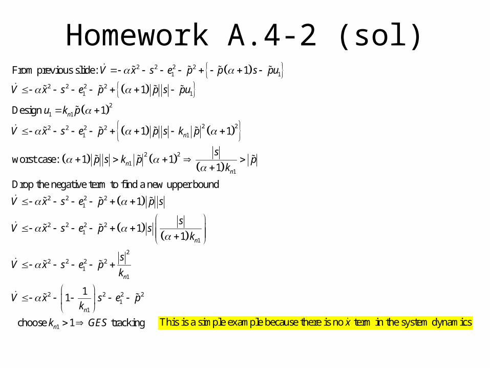
Homework A.4-2 (sol)
2 2 2 21 1
2 2 2 21 1
2
1 1
222 2 2 21 1
22
11
From previous slide: 1
1
Design 1
1 1
worst case: 1 11
Drop the negative te
n
n
nn
V x s e p p s pu
V x s e p p s pu
u k p
V x s e p p s k p
sp s k p p
k
2 2 2 21
2 2 2 21
1
2
2 2 2 21
1
2 2 2 21
1
1
rm to find a new upper bound
1
11
11
choose 1 tracking
n
n
n
n
V x s e p p s
sV x s e p s
k
sV x s e p
k
V x s e pk
k GES
This is a simple example because there is no term in the system dynamicsx
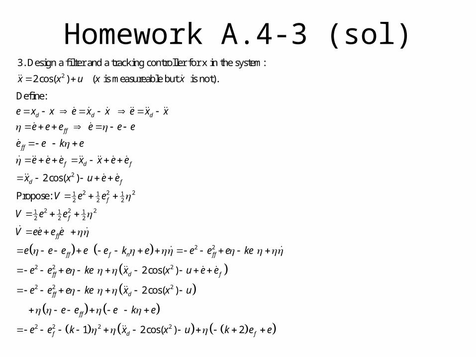
Homework A.4-3 (sol)
2
2 2 21 1 12 2 2
2 2 21 1 12 2 2
Define:
2cos( )
Propose:
d d d
f f
f f
f d f
d f
f
f
f f
f f f n
e x x e x x e x x
e e e e e e
e e k e
e e e x x e e
x x u e e
V e e
V e e
V ee e e
e e e e e k
2 2
2 2 2
2 2 2
2 2 2 2
2cos( )
2cos( )
1 2cos( ) 2
f f
f f d f
f f d
f f
f d f
e e e e ke
e e e ke x x u e e
e e e ke x x u
e e e k e
e e k x x u k e e
2
3. Design a filter and a tracking controller for x in the system:
2cos( ) ( is measureable but is not).x x u x x
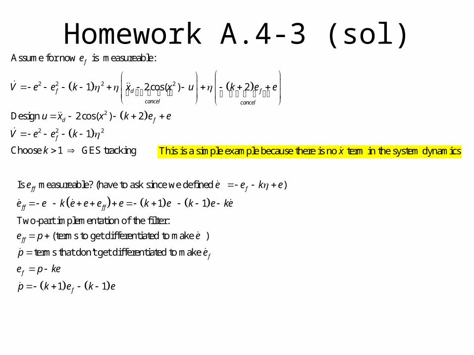
Homework A.4-3 (sol)
2 2 2 2
2
2 2 2
Assume for now is measureable:
1 2cos( ) 2
Design 2cos( ) 2
1
Choose 1 GES tracking
f
f d f
cancel cancel
d f
f
e
V e e k x x u k e e
u x x k e e
V e e k
k
This is a simple example because there is no term in the system dynamicsx
Is measureable? (have to ask since we defined )
1 1
Two-part implementation of the filter:
(terms to get differentiated to make )
terms that don't
f f f
f f f f
f f
e e e k e
e e k e e e e k e k e ke
e p e
p
get differentiated to make
1 1
f
f
f
e
e p ke
p k e k e