consumption and portfolio selection with labor income: a discrete-time approach

Math Meth Oper Res (1999) 50 :219±243

999

Consumption and portfolio selection with labor income:A discrete-time approach

Hyeng Keun Koo*

School of Business Administration, AJOU University, 5 Wonchun-Dong, Paldal-Gu, Suwon,442-749 South Korea (e-mail: [email protected])

Abstract. This paper studies the consumption and portfolio selection problemof an agent who is liquidity constrained and has uninsurable income risk in adiscrete time setting. It gives properties of optimal policies and presentsnumerical solutions. The paper, in particular, shows that liquidity constraintsand uninsurable income risk reduce consumption and investment in the riskyasset substantially from the levels for the case where no market imperfectionsexist. This paper also shows how the agent evaluates his or her human capitaland relates the evaluation to optimal decisions.

Key words: Consumption, portfolio selection, uninsurable risk, liquidity con-straints, non-linear optimization

1. Introduction

This paper investigates the e¨ects of uninsurable income risk and liquidityconstraints on optimal consumption and portfolio selection decision of aninvestor in a discrete-time setting. A companion paper (Koo 1998) investigatedthe problem in a continuous-time model and derived properties of optimalpolicies. In the paper we showed that the existence of uninsurable income riskand liquidity constraints lowers the subjective value of lifetime labor income.This paper continues the investigation by characterizing the optimal policieswhen the investor has no extra wealth than labor income (Proposition 3),

* I'd like to express my special thanks to John Campbell, Giuseppe Bertola, Angus Deaton,Avinash Dixit, and Kerry Back for their guidance and helpful suggestions. I also wish to thankPhil Dybvig, Miles Kimball, Guy Laroque, Lars Svensson, Harald Uhlig, Ingrid Werner forvaluable comments. Of course, all the remaining errors are mine.The author wishes to acknowledge ®nancial support of the Korean Research Foundation (No.304-452) made in the program year of 1999.

which has not been obtained in a continuous-time model. Furthermore, wesolve the model numerically and investigate properties of optimal policies byusing numerical examples. In particular, we show that the subjective value oflifetime labor income can be less than 10% of what it would be in the absenceof market imperfection.

Merton (1971) originally proposed a model of consumption and portfolioselection with labor income and solved it with constant absolute risk aversion(CARA) utility when labor income follows a Poisson process. Recently,Svensson and Werner (1993) have reconsidered the same problem but allowedincome to follow a Wiener process. They have shown that when an agent hasconstant absolute risk aversion but is not liquidity constrained, the existenceof uninsurable income risk lowers the implicit present value of future laborincome and thereby lowers consumption. In their model, however, the demandfor risky assets is not aëcted by uninsurable income risk. This is because thereis no wealth eëct on demand for risky assets when an agent has constantabsolute risk aversion. This paper focuses on optimal consumption and port-folio selection decisions made by economic agents who have constant relativerisk aversion (CRRA), and shows that uninsurable income risk and liquidityconstraints have signi®cant eëcts on both consumption and demand for riskyassets. Du½e et al. (1997) independently studied a continuous-time modelsimilar to the one in Koo (1998). They applied the viscosity solution techniqueto show properties of the value function (e.g., continuity, twice diëren-tiability, the validity of the Hamilton-Jacobi-Bellman equation). However,they did not investigate properties of optimal consumption and portfoliopolicies as we do here.

In another line of research, He and Pearson (1991) have proposed a mar-tingale approach to the consumption and portfolio selection problem in anincomplete market. He and PageÁs (1993), Cuoco (1997), Karoui and PicqueÂ(1995) have applied the martingale approach to a consumption and portfolioselection problem with labor income and liquidity constraints. However, theincome risk in their models is spanned by risks in ®nancial assets, i.e., liquidityconstraints are a unique source of market imperfection. In this paper incomerisk is not spanned by risks in ®nancial assets.

The paper proceeds as follows. Section 2 sets up a consumption and port-folio selection problem of an agent who receives a stream of labor income.Section 3 investigates the properties of optimal policies that can be derivedanalytically. Section 4 explains a procedure to solve the non-linear opti-mization problem numerically and presents numerical simulations. Section 5concludes and the appendix provides technical details.

2. The consumption and portfolio selection problem

The problem in this paper is the consumption and portfolio selectionproblem of an economic agent who receives a stream of labor income. Thereis an extensive literature on the consumption and savings problem with laborincome (see e.g., Skinner (1988), and Zeldes (1989a) for treatment of theproblem without liquidity constraints, and see Deaton (1991) for treatment ofthe problem with liquidity constraints). This paper extends the models to studythe consumption and portfolio selection problem of a liquidity constrainedagent.

220 H. K. Koo

Time is discrete t � 0; 1; 2; . . . ;T �T Uy�.1 The time to ®nal period isknown at time t � 0.

There is an economic agent whose preference over cosumption pro®les isgiven by the von Neumann-Morgenstern time separable utility function

u � EXT

t�0

�1� d�ÿtv�ct�( )

�1�

where d is the subjective rate of time preference, v�c� is given by the constantrelative risk aversion function

v�c�c1ÿg

1ÿ gif g0 1

log c if g � 1

8><>:The agent receives labor income yt at the beginning of time period �t; t� 1�.

We assume that labor is inelastically supplied.There are two assets, one riskless bond and one risky asset.2The real return on the riskless bond during a unit time interval �t; t� 1� is a

known constant R (i.e., the real interest rate is equal to r � Rÿ 1).The real return on the risky asset over the period �t; t� 1� is a random

variable with support �R;R�, 0UR < R < R <y and is denoted by ~Rt�1. Weassume the real return on the risky asset to be independently and identicallydistributed (iid) over time, and denote its mean and variance by E ~R and s2

R,respectively. We assume that E ~R > R, i.e., the equity premium is positive.There are no transaction costs for trading these ®nancial assets.

The constant risk-free rate assumption and the iid assumption on riskyasset returns imply that there does not occur any change in the agent'sinvestment opportunity set except that induced by the uncertain incomestream. The role of this assumption is to isolate the e¨ects of uninsurableincome risk on consumption and investment decisions from such other e¨ectsas those of time varying means and variances of asset returns.

The dollar amount invested in the risky asset for the period between t andt� 1 is denoted by pt. Given a consumption pro®le �ct� and a portfolio pro®le�pt�, ®nancial assets, At, evolve according to

At�1 � R�At � yt ÿ ct� � pt� ~Rt�1 ÿ R�: �2�Therefore, At means the assets that are carried over from the previous period(or endowed to the agent if t � 0).

The liquidity constraint considered in this paper takes the form

At V 0 for all t: �3�

1 A companion paper (Koo (1998)) has considered a similar problem in continuous time. Du½eet al. (1997) have independently considered a similar continous-time model and studied the exis-tence and uniqueness of an optimal policy.2 Generalization of theoretical results in the paper to the case where there are more than one riskyasset is not di½cult (see Koo (1998)), but it poses a new challenge for obtaining solutionsnumerically because it creates additional dimensions in the space of parameters to be determined.

Consumption and portfolio selection with labor income: A discrete-time approach 221

Credit rationing based on asymmetric information (see e.g., Stiglitz and Weiss(1981)) may provide a theoretical justi®cation for liquidity constraints.

Financial wealth (or cash on hand), xt, at time t is de®ned to be At � yt.3Liquidity constraint (3) requires that

0U ct U xt for all t; �4�

i.e., consumption does not exceed current ®nancial wealth.The liquidity constraint also requires a restriction on the amount invested

in the risky asset. The constraint will be satis®ed if the agent faces a marginrequirement and short-selling restriction of the following form:

ÿo�xt ÿ ct�U pt Uo�xt ÿ ct� with oUR

Rÿ R; oU

R

Rÿ R�5�

where R is the lower bound and R is the upper bound for the real returns onthe risky asset. In fact, the combination of the consumption constraint in (4)and the short-selling constraint in (5) with o � R=�RÿR� and o � R=�RÿR�is equivalent to the liquidity constraint in (3). Therefore, if the two constraintsin (4) and (5) are satis®ed, the liquidity constraint is automatically satis®ed.

The agent's value function V is de®ned to be the maximized value ofexpected utility subject to (2), (4), and (5). Under suitable regularity con-ditions there exists a unique optimal consumption and investment policy.4Throughout the paper we will assume the existence and uniqueness of anoptimal policy.

3. Properties of optimal policies

In this section we study properties of optimal policies. Empirical studies ofmicroeconomic and macroeconomic income processes generally agree thatincome shocks have two components, a permanent component and a transi-tory component (see e.g., Hall and Mishkin (1982), MaCurdy (1982)). Insubsection 3.1 we consider a polar case where income shocks are all perma-nent, and in subsection 3.2 we consider the general case where income shockshave both permanent and transitory components.

3.1 Permanent income shocks

This subsection studies the case where income shocks are permanent. Namely,In this subsection we make the following assumption:

3 Here we use the terms ®nancial assets and ®nancial wealth (or cash on hand ) to mean twodi¨erent things. The former means the assets that are endowed or carried over from the previousperiod, and the latter means the sum of these ®nancial assets and current labor income. Thetwo are equal in continuous time, since income received over an in®nitesimal time period isin®nitesimally small.4 A su½cient condition for the existence and uniqueness of a policy is available upon request fromthe reader.

222 H. K. Koo

Assumption 1: The joint distribution of growth rate of income yt�1=yt and thereturn on the risky asset is iid.

We denote the iid random variable yt�1=yt by ~g, and denote then meanand variance of log ~g by g and s2

g , respectively. The covariance between log ~Rand log ~g is denoted by sR;g.

Assumption 1 implies that the agent's optimal consumption and investmentin the risky asset are both homogeneous functions of degree 1 in the current®nancial wealth xt and labor income yt. This implies that the dimension of theproblem can be reduced by one as shown in the following lemma:

Lemma 1: Suppose that Assumption 1 is valid. Let c�xt� denote the agent'soptimal consumption and p�xt� denote the agent's optimal investment in therisky asset when yt � 1.5

(i) Then the optimal consumption and portfolio policy is given by

ct � c�zt�yt pt � p�zt�yt

where zt is the ratio de®ned by

zt 1xt

yt

:

(ii) The value function V is homogeneous of degree 1ÿ g in ®nancial wealth,xt, and labor income, yt, where g is the coe½cient of relative risk aversion of theperiod utility function. Let f�z� be the function de®ned by f�z�1V�z; 1�. Thenthe value function can be expressed as

V�xt; yt� �f�zt�y1ÿg

t if g0 1

f�zt� � 1� dÿ 1=�1� d�Tÿt

dlog yt if g � 1

8>><>>: :

Proof: See Appendix.6 k

The following proposition illustrates the agent's implicit evaluation oflifetime labor income:

Proposition 1: Suppose that Assumption 1 is valid. Suppose further thatE ~gÿg� ~Rÿ R�0 0.7

(i) Then, for y > 0, the value function V�x; y� has ®rst-order partialderivatives.

5 The optimal policies and value function depend on the time to maturity T ÿ t� 1. However,for simplicity, we will use notation which does not explicitly show this dependence, unless there isa possibility of confusion. Namely, we will use c�xt� or V�xt; yt� instead of c�xt;T ÿ t� 1� orV�xt; yt;T ÿ t� 1�.6 Proofs of lemmas and propositions in this paper are contained in Appendix that is availablefrom the author upon request.7 The assumption that E ~gÿg� ~Rÿ R�0 0 is a technical condition that guarantees the uniquenessof a solution to the ®rst order conditions (see equation (14) in section 4.1).


(ii) Let the marginal rate of substitution p between labor income and®nancial wealth be de®ned by

p1Vy�x; y�Vx�x; y� ;

and let q be de®ned by

q1

�1ÿ g� V�x; y��x� p�z�y�1ÿg

if g0 1

ed=�1�dÿ1=�1�d�Tÿt�V�x; y��x� py� if g � 1

8>>>><>>>>: :

Then, p and q are functions of z1 x=y, and the value function can berepresented as8

V�x; y� �

q�z�1ÿ g

�x� p�z�y�1ÿg if g0 1

1� dÿ 1=�1� d�Tÿt

dlog q�z��x� p�z�y� if g � 1

8>>><>>>: :

(iii) Let ct be optimal consumption at time t. Then, the envelope theorem

Vx�xt; yt� � cÿgt

is true, and optimal consumption takes the form

ct �q�zt�ÿ�1=g��xt � p�zt�yt� if g0 1

d

1� dÿ 1=�1� d�Tÿt�xt � p�zt�yt� if g � 1

8>><>>: :

The quantity p�zt�yt in Proposition 1 is the present value of lifetime laborincome evaluated by the agent; therefore, it can be regarded as the implicitvalue of human capital. Proposition 1 shows the importance of the implicitvalue of human capital in the agent's optimal decisions. Namely, Proposition1 (ii) shows that the value function can be represented as a homogeneousfunction of the sum of ®nancial wealth and the implicit value of human capital(we will call this sum as the agent's implicit total wealth). Proposition 1 (iii)shows that optimal consumption is a fraction (a constant fraction if g � 1,and a time-varying fraction if g0 1) of implicit total wealth. The life cycle-permanent income hypothesis (LCPIH) for consumption asserts that con-sumption is a function of the present value of lifetime income (Modigliani andBrumberg (1954) and Friedman (1957)). Therefore, Proposition 1 (iii) can beregarded as an extension of the LCPIH to the case where the agent is liquidityconstrained and has uninsurable income risk.

8 Davis and Norman ®rst used this representation (1990).

224 H. K. Koo

In the following example, we consider the case where there is nouninsurable income risk and the ®nancial market is perfect.

Example 1: In the case where labor income is deterministic and there is noborrowing constraint nor short-selling restriction (i.e., the ®nancial marketis perfect), the value of human capital is given as the present value of futurelabor income

p�zt�yt �Ryt

Rÿ Gif R > G

y otherwise

8<: �6�

where G � eg is the deterministic growth rate of income in this case. There-

fore, p�z�1 G

Rÿ Gif R > G, and human capital is a perfect substitute for

®nancial wealth. The value function can be regarded as a function of a singlevariable, i.e., wealth W, which is the sum of ®nancial wealth and the presentvalue of future labor income. Therefore, q�z� is also a constant.

In this case both optimal consumption and investment in the risky asset areequal to constant fractions of the sum of ®nancial wealth and the presentvalue of future labor income. k

If there exists uninsurable income risk and liquidity constraints, then p�z�and q�z� in Proposition 1, in general, vary over time. The following proposi-tion gives the properties of these functions.

Proposition 2: Suppose that Assumption 1 is valid, and E ~gÿg� ~Rÿ R�0 0.Suppose also that the value function is twice-diërentiable9 on f�x; y� : y > 0and 1U a < x=y < bg.10 Then the following are true:

(i) The marginal rate of substitution p�z� between ®nancial wealth andcurrent labor income is a monotone non-decreasing function of the ratio of®nancial wealth to current labor income z, for a < z < b, i.e.,

p 0�z�V 0 for a < z < b:

(ii) The function q�z� satis®es the following diërential equation for a <z < b

q 0�z�q�z� �

ÿ �1ÿ g�p 0�z�z� p�z� if g0 1

ÿ p 0�z�z� p�z� if g � 1

8>>>><>>>>: :

9 The assumptions of Proposition 2 include that of twice-diërentiability of the value function. Itcan be shown that under certain regularity conditions the value function for the ®nite-horizonproblem has absolutely continuous ®rst-order partial derivatives and therefore has second-orderpartial derivatives almost everywhere. Koo (1998) has shown that under certain regularity con-ditions the value function for the in®nite-horizon problem is continuously twice-diërentiable ifx > 0 and y > 0 and time is continuous.10 Due to the liquidity constraint At V 0 in (3), zt � xt=yt V 1.


(iii) Let implicit total wealth be de®ned to be x� p�z�y. Then, the ratio ofoptimal consumption to implicit total wealth is constant if g � 1, monotone non-increasing in z if g > 1, and monotone non-decreasing in z if g < 1.

Therefore, ceteris paribus, the implicit value of human capital increases as®nancial wealth increases. This is intuitive in the sense that as the ratio of®nancial wealth to income increase, the e¨ects of uninsurable risk and theliquidity constraints become smaller, and therefore, human capital is morevaluable to the agent. Results similar to the Propositions 1 and 2 are alsoobtained in Koo (1998).

We now want to discuss optimal consumption when the agent doesnot have any assets carried over from the previous period, i.e., At � 0 (equiv-alently, xt � yt or zt � 1). Deaton discusses the same problem in the contextof a consumption and savings problem and derives a condition under whichthe agent consumes all current ®nancial wealth (see condition (27) in Deaton(1991), see also Theorem 1 in Deaton and Laroque (1992)). The followingproposition characterizes optimal consumption when At � 0 for the con-sumption and portfolio selection problem. In particular, it shows that con-sumption is more likely to be lower than ®nancial wealth in the case where theagent's investment opportunity set has both the riskless and risky assets thanin the case where the investment opportunity set has only the riskless asset:

Proposition 3: Suppose that Assumption 1 is valid and that E ~gÿg� ~Rÿ R�0 0.Let o� � o if E ~gÿg� ~Rÿ R� > 0 and o� � ÿo if E ~gÿg� ~Rÿ R� < 0.

(i) Then optimal consumption at zt � xt=yt � 1 is equal to current ®nancialwealth if and only if

1

1� dE~gÿg�R� o�� ~Rÿ R��U 1:

Further, if the above inequality is valid, then there exists ~z > 1 such that theoptimal ratio of the risky asset holdings to total investment is equal to o� for all1 < zt U ~z.

(ii) Optimal consumption is strictly less than current ®nancial wealth for allzt � xt=yt V 1 if

1

1� dE~gÿg�R� o�� ~Rÿ R�� > 1:

An intuitive explanation of Proposition 3 (i) can be given as fol-lows: If the inequality in Proposition 3 (i) is valid, then the quantity,

1

1� dE~gÿg�R� o�� ~Rÿ R��, is equal to the discounted expected value of the

future marginal utility of money when xt � yt � 1. Suppose now that thisdiscounted expected value of the future marginal utility of money is smallerthan the current marginal utility of money. Then the agent would want toconsume more than current ®nancial wealth if there were no liquidity con-straints. Therefore, in the presence of liquidity constraints, the agent's optimalconsumption would be equal to current ®nancial wealth.

Proposition 3 (ii) shows that if the inequality in Proposition 3 (i) is reversed,then it provides a su½cient condition for optimal consumption to be strictly

226 H. K. Koo

smaller than current ®nancial wealth.11 If, in particular, labor income and thereturn on the risky asset have zero correlation, then the condition becomessimpler and takes the following form:

1

1� dE~gÿg�R� o�E ~Rÿ R�� > 1: �7�

If ~g is lognormally distributed,12 so that ln ~g is N�g; s2g� and we make the

usual approximation �1� d�ea � 1� d� a, then (7) becomes

rÿ d� om

g� g

2s2

g > g; �8�

where r � Rÿ 1 is the risk-free rate and m � E ~Rÿ R is the return premium onthe risky asset. The left-hand side of inequality (8) is di¨erent from that ofcondition (27) in Deaton (1991) by om=g. Therefore, inequality (8) shows thatconsumption is more likely to be lower than ®nancial wealth in the case wherethe agent's investment opportunity set has both the riskless and risky assetsthan in the case where the investment opportunity set has only the risklessasset. Intuitively, the existence of a broader opportunity to invest increases theagent's marginal utility of money, and this tends to reduce consumption below®nancial wealth.

Proposition 3 (i) also gives a characterization of the agent's investment inthe risky asset when ®nancial wealth is small. The characterization is provenonly for the case where the inequality in Proposition 3 (i) is valid, but Iconjecture that it is generally valid for the other case as well (all numericalsimulations in section 4 con®rm this characterization). The characterizationsays that when ®nancial wealth is small, the agent invests in the risky assetup to the maximum limit if E~gÿg� ~Rÿ R� > 0, and does not invest in therisky asset �o � 0� or shorts it up to the maximum limit �ÿo < 0� ifE ~gÿg� ~Rÿ R� < 0. If log ~R and log ~g are jointly normally distributed and wemake the usual approximation ea � 1� a and ignore terms of the secondorder, the conditions can be expressed as:

E ~Rÿ R > �<�gsR;g �9�

where sR;g is the covariance between log ~R and log ~g. The right-hand side of(9) can be regarded as the implicit risk-premium on human capital. Therefore,condition (9) says that when ®nancial wealth is small, the agent buys the riskyasset up to the maximum limit if the return premium on the risky asset isgreater than the implicit risk-premium on human capital, and invests nothingin the risky asset or shorts it up to the maximum limit if the return premiumon the risky asset is smaller than the implicit risk-premium on human capital.

A result in continuous time provides a deeper insight about portfolioselection. Koo (1998) has shown that in continuous time the optimal propor-

11 Proposition 3 (ii) gives a su½cient condition for z � 0 to be a re¯ecting barrier.12 The lognormal assumption on the risky asset's returns does not exactly match with theprevious assumption that the returns have a compact support that is bounded above by a positivereal number. But if we truncate the lognormal distribution appropriately, then inequality (7) canbe made approximately valid with only a small error.


tion o of the investment in the risky asset is given by

o �o� if ÿoUo�Uo

o if o� > o

ÿo if o� < ÿo

8<: �10�

where

o� � E ~Rÿ R

s2R

ÿ gsR;g

s2R

� �1

g� p 0�z��

1� p�z�z

� �� sR;g

s2R

:

Equation (10) admits the following interpretation: the agent does not con-sider only ®nancial wealth when making investment decisions, but the agentcalculates also the implicit value of human capital and wants to invest part ofthis implicit value in the risky asset and to hedge risk in the implicit value.Note that the coe½cient of relative risk aversion is adjusted upward by p 0�z�.

Therefore, when ®nancial wealth is small and the return premium on therisky asset is greater than the implicit risk-premium on human capital, theoptimal fraction of human capital to be invested in the risky asset is equal tothe maximum limit, because the implicit value of human capital is muchgreater than the currently saved money. If the return premium on the riskyasset is smaller than the implicit risk-premium on human capital, the agentwants to sell short the risky asset (if allowed) as a hedge against risk in humancapital; when ®nancial wealth is small, the amount sold short is equal to themaximum possible limit.

3.2 Permanent and transitory income shocks

Main results in the previous subsection can be extended to the case where in-come shocks have both permanent and transitory components. Namely, if onetakes a discrete approximation for the transitory component in the incomeshocks, then the functions p and q can be de®ned similarly to the way thatthey are de®ned in the previous subsection and one can analyze the optimalpolicy by investigating the implicit values of human capital. For example, letus suppose that labor income yt follows the following process13:

yt�1 � yt�1st�1 �11�where the joint distribution of yt�1=y, ~Rt�1, and st�1 are iid, and st takes valuesamong �s�1�; s�2�; . . . ; s�N��. We assume that yt and st are observable sepa-rately. The component yt represents part of income which has a perment e¨ecton future income, and the component st represents a temporary shock.

The value function can now be written as V�xt; yt; st�. Then, the marginalrate of subsitution p can be de®ned by

p1Vy�xt; yt; st�Vx�xt; yt; st� : �12�

13 Zeldes (1989a) has considered a similar process.

228 H. K. Koo

The function q can be de®ned similarly. Then, by assuming appropriate dif-ferentiability, it can be shown that p�. . . ; s�i�� is a non-decreasing functionof z1 x=y for each i � 1; 2; . . . ;N (i.e., Proposition 2 (i) is valid). That is,generally, the implicit value of human capital increases for the same level oftransitory income shocks, as ®nancial wealth increases. Assuming the envelopetheorem Vx�xt; yt; st� � c

ÿgt , optimal consumption takes the form in Proposi-

tion 1 (iii), and Proposition 2 (ii) and (iii) are valid.14

4. Numerical simulations

In this section we will present numerical solutions to the intertemporal con-sumption and investment problem. Subsection 4.1 will explain the numericalmethod and subsection 4.2 will present numerical solutions.

4.1 The numerical method

In this subsection we explain the numerical method to obtain solutions in thissubsection. We consider only the case where income shocks are permanent(see section 3.1). The method can be easily extended to the case where incomeshocks have both permanent and transitory components.

We use notation introduced at the beginning of section 3, but the notationshows the time horizon of the consumption and portfolio selection problemexplicitly: fT �z�1VT�z; 1�, cT�z� is the optimal consumption and pT�z� isthe optimal investment in the risky asset when x � z and y � 1 and there are�T � 1� periods. We also use the notation oT�z� for the optimal ratio ofthe amount invested in the risky asset to total investment, i.e., oT �z�1 pT �z�=�zÿ cT�z�� if cT�z� < z.

A typical procedure used to solve the ®nite horizon problem is backwardinduction, which consists of updating the value function by the following rule:

fT�z�� maxs:t:�4�;&�5�

vc

y

� �� 1

1�dEfTÿ1 1� R zÿ c

y

� ��p

y

� �~gÿ1

� �~g1ÿg

� �; �13�

the ®rst order conditions for problem (13) can now be stated as

f 0T�z� � max

�zÿg;

1

1� dEf 0Tÿ1f1� �R� oT�z�� ~Rÿ R��zÿ f 0T �z�ÿ1=g�~gÿ1g

� ~gÿg�R� oT �z�� ~Rÿ R��

�14�

oT�z� � o if Ef 0Tÿ1f1� �R� o� ~Rÿ R��zÿ f 0Tÿ1�z�ÿ1=g�~gÿ1g

� ~gÿg� ~Rÿ R� > 0;

14 We have not obtained a proof of the envelope theorem in full generality.


oT �z� � ÿo if Ef 0Tÿ1f1� �Rÿ o� ~Rÿ R��zÿ f 0Tÿ1�z�ÿ1=g�~gÿ1g� ~gÿg� ~Rÿ R� < 0;

Ef 0Tÿ1f1� �R� oT�z�� ~Rÿ R��zÿ f 0Tÿ1�z�ÿ1=g�~gÿ1g� ~gÿg� ~Rÿ R� � 0 otherwise:

The numerical solutions to ®nite-horizon problems can be obtained by usingthe ®rst order conditions in (14). The solutions to in®nite-horizon problemscan be obtained by taking the limits of consumption and portfolio policies for®nite-horizon problems.15

When modelling the returns on the risky asset and income growth rates,we assume that their logarithms are jointly normally distributed (truncatedappropriately, if necessary) and use the Gaussian quadrature method to cal-culate expectations (see Tauchen and Hussey (1991)).

We choose a grid f1 � z0; z1; . . . ; zMg for the ®nancial wealth to incomeratio z. Each iteration step requires knowledge of the marginal utility of moneyfunction f 0T�z� over �1; z 0�, where z 0 is the maximum ratio of ®nancial wealthto income in the next period. Therefore, it is necessary to extrapolate thefunction which is obtained on the interval �1; zM � to get the values over�zM ; z

0�. We use an extrapolation method based on the representation of thevalue function in Proposition 1. The envelope theorem (Proposition 1 (iii))implies that f 0�z� � q�z��z� p�z��ÿg and we extrapolate the function assum-ing that p�z� and q�z� are constant beyond zM . This extrapolation method hasthe following justi®cations. First, as the time interval between consecutiveperiods shrinks, the di¨erence between z 0 and zM converges to zero. So theassumption that p and q do not change over the interval �z1; zM � is not harmfulif the time intervals are small enough. Second, in continuous time (Koo(1998)) we have shown that under suitable regularity conditions the derivativesof the functions p and q approach zero as z gets large. Therefore, if zM is largeenough, the assumption that p and q are constant over �zM ; z

0� does not seemharmful. Numerical experiment showed that the convergence of the numericalalgorithm for the in®nite-horizon problem using this extrapolation methodwas fairly stable. For the parameter values used in the simulations presentedin this section, the algorithm converged in shorter than 250 simulated years.

4.2 Numerical results

For numerical simulations we take the risk-free rate to be 1% (i.e., R � 1:01),the historical average real interest rate in the U.S. We assume the expectedrate of return on the risky asset to be 7% (i.e., E ~R � 1:07), adding the histor-ical average risk premium 6% to the risk-free rate. The standard deviation ofthe return on the risky asset is set to be 20%, the historical standard deviationof equity returns in the U.S.

15 By extending a method in Deaton and Laroque (1992) it can be shown that the iterationprocedure gives a correct solution to the ®nite-horizon problems. It can also be shown thatoptimal policies for ®nite-horizon problems converge to the optimal policy for in®nite-horizonproblems.

230 H. K. Koo

The values chosen for the expected growth rate of income are 0% and 2%.If the expected growth rate is 0%, the impicit value of human capital is ®nitewhen the market is perfect (see Example 1 in section 3), so this case facilitatesthe comparison between the optimal policies for the liquidity-constrained casewith those for the perfect-market case. The value 2% is consistent with thehistorical average growth rate of national income in the U.S. The valueschosen for the standard deviation of the growth rate of income are 0%, 10%,and 15%. Both 10% and 15% are consistent with estimates of the magnitudeof permanent shocks to individual income in Hall and Mishkin (1982) andMaCurdy (1982).

We assume that the correlation rR;g between the growth rate of incomeand the return on the risky asset is equal to zero. This assumption allows usto focus on the role of uninsurable income risk in optimal consumption andinvestment decisions (see Koo (1998) for treatment of the case where rR;g 0 0).

The subjective discount rate is taken to be 10%, which indicates that theeconomic agent is relatively impatient. The values chosen for the coe½cient ofrelative risk aversion g are 0.9, 3, and 5.

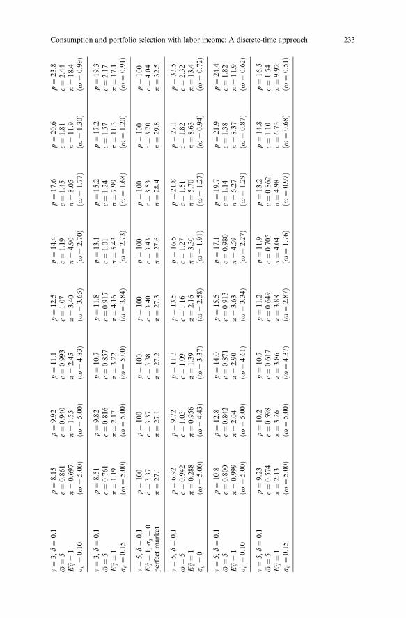
Tables I±III give simulation results for the case where income shocks arepermanent and Table IV gives simulation results for the case where incomeshocks have both permanent and transitory components. The values of con-sumption, c, and investment in the risky asset, p, in Tables I±III are the ratiosof optimal consumption and investment in the risky asset to annual income,respectively. The values of c in Table IV are the ratios of optimal consumptionto the permanent component of annual income (i.e. annualized value of yt).The notation p denotes the implicit value of human capital when (the perma-nent component of ) annual income is equal to 1. The notation A in the tablesdenotes the value of ®nancial assets carried over from the previous period (or®nancial assets that are endowed to the agent if t � 0), X denotes ®nancialwealth, and Y denotes annual income.

Table I: In Table I, we consider optimal consumption and investment policiesfor the case where the margin requirement and short-selling restriction arefairly generous. Namely, Table I gives the implicit value of human capital,optimal consumption, and optimal investment in the risky asset when o �o � 5, income shocks are permanent, and the time horizon is in®nite. Weassume that the expected growth rate of income is equal to 0% in this table,and this assumption allows us to compare the case where the agent is liquidityconstrained with the case where the ®nancial market is perfect. Graphicalrepresentations of part of Table I are given in Figure 1, Figure 2, and Figure 3.

Table I shows that both consumption and investment in the risky assetare unrealistically high when the ®nancial market is perfect. Even for a highvalue of relative risk aversion g, consumption is three times as large as annualincome and investment in the risky asset is twenty-seven times as large asannual income when At � 0. The high level of consumption can partly beexplained by the assumption that the agent is impatient (d � 10%), but themain reason for the high level of consumption and large investment in therisky asset is because the value of human capital is very large. With a freeborrowing and lending opportunity at the low risk-free rate 1%, the presentvalue of future labor income is 100 times as large as annual labor income, andthe agent wants to consume an optimal fraction of this present value and in-vest an optimal fraction of the present value in the risky asset. In particular,


Ta

ble

I.T

he

imp

lici

tv

alu

eo

fh

um

an

cap

ita

l,o

pti

mal

con

sum

pti

on

,an

do

pti

mal

inves

tmen

tin

the

risk

yass

et(p

erm

an

ent

inco

me

sho

cks,

in®

nit

eh

ori

zon

)

pa

ram

eter

va

lues

A Y�

0A Y�

1 4

A Y�

1 2

A Y�

1A Y�

2A Y�

5A Y�

10

A Y�

20

g�

0:9

,d�

0:1

p�

10

0p�

100

p�

100

p�

100

p�

100

p�

100

p�

100

p�

100

E~ g�

1,

sg�

0c�

9:8

8c�

9:9

1c�

9:9

3c�

9:9

8c�

10:

1c�

10:4

c�

10:

9c�

11:

9p

erfe

ctm

ark

etp�

15

5p�

155

p�

156

p�

157

p�

158

p�

163

p�

171

p�

186

g�

0:9

,d�

0:1

p�

7:6

2p�

8:2

7p�

8:8

2p�

9:6

8p�

10:9

p�

12:

8p�

14:

6p�

16:4

o�

5c�

0:7

09

c�

0:7

98

c�

0:8

76

c�

1:0

1c�

1:2

3c�

1:7

1c�

2:3

8c�

3:5

3E

~ g�

1p�

1:4

5p�

2:2

6p�

3:1

2p�

4:9

5p�

8:3

7p�

15:

5p�

25:9

p�

45:

1s

g�

0�o�

5:0

0�

�o�

5:0

0��o�

5:0

0��o�

5:0

0��o�

4:7

2��o�

3:6

1��o�

3:0

0��o�

2:5

8�

g�

0:9

,d�

0:1

p�

7:4

4p�

8:0

7p�

8:6

0p�

9:4

3p�

10:6

p�

12:

4p�

14:

1p�

15:8

o�

5c�

0:6

94

c�

0:7

81

c�

0:8

58

c�

0:9

89

c�

1:2

0c�

1:6

8c�

2:3

4c�

3:4

8E

~ g�

1p�

1:5

3p�

2:3

4p�

3:2

1p�

5:0

6p�

8:4

8p�

15:

5p�

25:8

p�

44:

7s

g�

0:1

0�o�

5:0

0�

�o�

5:0

0��o�

5:0

0��o�

5:0

0��o�

4:7

1��o�

3:5

9��o�

2:9

8��o�

2:5

5�

g�

0:9

,d�

0:1

p�

7:2

2p�

7:8

3p�

8:3

4p�

9:1

3p�

10:2

p�

12:

0p�

13:

6p�

15:1

o�

5c�

0:6

76

c�

0:7

60

c�

0:8

35

c�

0:9

62

c�

1:1

7c�

1:6

4c�

2:2

9c�

3:4

2E

~ g�

1p�

1:6

2p�

2:4

5p�

3:3

3p�

5:1

9p�

8:6

0p�

15:

6p�

25:7

p�

44:

3s

g�

0:1

5�o�

5:0

0�

�o�

5:0

0��o�

5:0

0��o�

5:0

0��o�

4:6

9��o�

3:5

7��o�

2:9

5��o�

2:5

2�

g�

3,

d�

0:1

p�

10

0p�

100

p�

100

p�

100

p�

100

p�

100

p�

100

p�

100

E~ g�

1,

sg�

0c�

4:7

5c�

4:7

7c�

4:7

8c�

4:8

0c�

4:8

5c�

4:9

9c�

5:2

3c�

5:7

0p

erfe

ctm

ark

etp�

45:7

p�

45:

8p�

46:

0p�

46:2

p�

46:

6p�

48:

0p�

50:3

p�

54:

9

g�

3,

d�

0:1

p�

7:2

7p�

9:2

9p�

10:

6p�

12:

2p�

14:5

p�

18:

5p�

22:

6p�

27:3

o�

5c�

0:9

14

c�

1:0

2c�

1:0

8c�

1:1

8c�

1:3

2c�

1:6

3c�

2:0

3c�

2:7

1E

~ g�

1p�

0:4

29

p�

1:1

7p�

1:8

5p�

2:7

9p�

4:2

9p�

7:6

1p�

11:8

p�

19:

0s

g�

0�o�

5:0

0�

�o�

5:0

0��o�

4:4

2��o�

3:3

9��o�

2:5

5��o�

1:7

4��o�

1:3

2��o�

1:0

4�

232 H. K. Koo

g�

3,

d�

0:1

p�

8:1

5p�

9:9

2p�

11:

1p�

12:

5p�

14:4

p�

17:

6p�

20:

6p�

23:8

o�

5c�

0:8

61

c�

0:9

40

c�

0:9

93

c�

1:0

7c�

1:1

9c�

1:4

5c�

1:8

1c�

2:4

4E

~ g�

1p�

0:6

97

p�

1:5

5p�

2:4

5p�

3:4

0p�

4:9

0p�

8:0

5p�

11:9

p�

18:

4s

g�

0:1

0�o�

5:0

0�

�o�

5:0

0��o�

4:8

3��o�

3:6

5��o�

2:7

0��o�

1:7

7��o�

1:3

0��o�

0:9

9�

g�

3,

d�

0:1

p�

8:5

1p�

9:8

2p�

10:

7p�

11:

8p�

13:1

p�

15:

2p�

17:

2p�

19:3

o�

5c�

0:7

61

c�

0:8

16

c�

0:8

57

c�

0:9

17

c�

1:0

1c�

1:2

4c�

1:5

7c�

2:1

7E

~ g�

1p�

1:1

9p�

2:1

7p�

3:2

2p�

4:1

6p�

5:4

3p�

7:9

9p�

11:3

p�

17:

1s

g�

0:1

5�o�

5:0

0�

�o�

5:0

0��o�

5:0

0��o�

3:8

4��o�

2:7

3��o�

1:6

8��o�

1:2

0��o�

0:9

1�

g�

5,

d�

0:1

p�

10

0p�

100

p�

100

p�

100

p�

100

p�

100

p�

100

p�

100

E~ g�

1,

sg�

0c�

3:3

7c�

3:3

7c�

3:3

8c�

3:4

0c�

3:4

3c�

3:5

3c�

3:7

0c�

4:0

4p

erfe

ctm

ark

etp�

27:1

p�

27:

1p�

27:

2p�

27:3

p�

27:

6p�

28:

4p�

29:8

p�

32:

5

g�

5,

d�

0:1

p�

6:9

2p�

9:7

2p�

11:

3p�

13:

5p�

16:5

p�

21:

8p�

27:

1p�

33:5

o�

5c�

0:9

42

c�

1:0

3c�

1:0

9c�

1:1

6c�

1:2

7c�

1:5

1c�

1:8

2c�

2:3

2E

~ g�

1p�

0:2

88

p�

0:9

56

p�

1:3

9p�

2:1

6p�

3:3

0p�

5:7

0p�

8:6

3p�

13:

4s

g�

0�o�

5:0

0�

�o�

4:4

3��o�

3:3

7��o�

2:5

8��o�

1:9

1��o�

1:2

7��o�

0:9

4��o�

0:7

2�

g�

5,

d�

0:1

p�

10:

8p�

12:

8p�

14:

0p�

15:

5p�

17:1

p�

19:

7p�

21:

9p�

24:4

o�

5c�

0:8

00

c�

0:8

42

c�

0:8

71

c�

0:9

13

c�

0:9

80

c�

1:1

4c�

1:3

8c�

1:8

2E

~ g�

1p�

0:9

99

p�

2:0

4p�

2:9

0p�

3:6

3p�

4:5

9p�

6:2

7p�

8:3

7p�

11:

9s

g�

0:1

0�o�

5:0

0�

�o�

5:0

0��o�

4:6

1��o�

3:3

4��o�

2:2

7��o�

1:2

9��o�

0:8

7��o�

0:6

2�

g�

5,

d�

0:1

p�

9:2

3p�

10:

2p�

10:

7p�

11:

2p�

11:9

p�

13:

2p�

14:

8p�

16:5

o�

5c�

0:5

74

c�

0:5

98

c�

0:6

17

c�

0:6

49

c�

0:7

05

c�

0:8

62

c�

1:1

0c�

1:5

4E

~ g�

1p�

2:1

3p�

3:2

6p�

3:8

6p�

3:8

8p�

4:0

4p�

4:9

8p�

6:7

3p�

9:9

2s

g�

0:1

5�o�

5:0

0�

�o�

5:0

0��o�

4:3

7��o�

2:8

7��o�

1:7

6��o�

0:9

7��o�

0:6

8��o�

0:5

1�


the values for the investment in the risky asset show that the perfect marketassumption would generate unrealistic implications if it is applied to studyempirical asset prices (see Mehra and Prescott (1985)).

According to Table I, both consumption and investment in the risky assetare substantially lower in the case where the agent is liquidity constrainedthan in the case where the ®nancial market is perfect. For all the di¨erentvalues of relative risk aversion, the reduction in consumption due to liquidityconstraints is larger than 66%, and the reduction in the investment in the riskyasset is larger than 90%, when ®nancial assets are smaller than current laborincome. The e¨ects of liquidity constraints are large even when ®nancial assetsare large. When the total value of ®nancial assets is 20 times as large as annualincome, the reduction in consumption due to liquidity constraints is largerthan 40% and the reduction in the investment in the risky asset is larger than60% for all the values of relative risk aversion considered in the table. If the®nancial market is perfect, then even at this high level of ®nancial assets, thevalue of human capital is much larger than (5 times as large as) the value of®nancial assets, therefore, the agent invests an amount much larger than thecurrent value of ®nancial assets (an amount larger by 803% if g � 0:9, by157% if g � 3, and by 51% if g � 5) in the risky asset borrowing from futurelabor income. But this large-scale risk-taking is not optimal in the presence ofliquidity constraints because a bad investment outcome would severely restrictthe agent's consumption and investment.

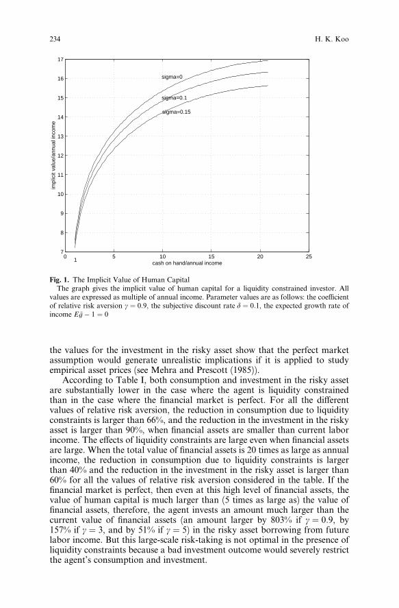
Fig. 1. The Implicit Value of Human CapitalThe graph gives the implicit value of human capital for a liquidity constrained investor. All

values are expressed as multiple of annual income. Parameter values are as follows: the coe½cientof relative risk aversion g � 0:9, the subjective discount rate d � 0:1, the expected growth rate ofincome E ~gÿ 1 � 0

0 5 10 15 20 257

8

9

10

11

12

13

14

15

16

17

cash on hand/annual income

impl

icit

valu

e/an

nual

inco

me

sigma=0

sigma=0.1

sigma=0.15

1

234 H. K. Koo

All the numerical simulations for the liquidity-constrained case in Table Ishow that consumption is strictly smaller than current income. This con®rmsthe theoretical result in Proposition 3. Namely, the expected return on invest-ment is high in the presence of the risky asset, and this high expected returninduces the agent to save a non-zero amount even when ®nancial assets aresmall.

Table I also shows that consumption declines monotonically when incomerisk increases. This result is consistent with the ®ndings by earlier researchersthat, when income risk increases, agents become more prudent and increasesavings to prepare against a possible decline in income (see e.g., DreÁze andModigliani (1972), Campbell (1987), Kimball (1990), and Deaton (1991)).

Table I shows that the implicit value of human capital is increasing as theratio of ®nancial assets to labor income increases, con®rming the theoreticalresult in Proposition 2.

Table I shows that the agent invests in the risky asset up to the maxi-mum limit shorting the riskless asset when ®nancial assets are small. This isconsistent with the theoretical discussion about asset demand followingProposition 3.

Table II: Table II shows the implicit value of human capital, optimal con-sumption, and investment in the risky asset for various values of the upperbound o of the proportion that can be invested in the risky asset. In the 5th

Fig. 2. Optimal ConsumptionThe graph gives the optimal consumption for a liquidity constrained investor. All values are

expressed as multiple of annual income. Parameter values are as follows: the coe½cient of relativerisk aversion g � 0:9, the subjective discount rate d � 0:1, the expected growth rate of incomeE ~gÿ 1 � 0


and 6th rows in the table, we present also the result of a numerical simulationin which the borrowing rate RB, which is applied when the risky asset is pur-chased on margin, is higher than the lending rate, R by 3%. The time horizonis in®nite and income shocks are permanent. The expected annual growth rateof labor income is 2% and the coe½cient of relative risk aversion g is 5.

This table, therefore, shows the e¨ects of a change in the investmentopportunity on the agent's optimal decisions. The table shows that when thestandard deviation sg of the growth rate of income is 10%, an increase in theupper bound o reduces consumption and the implicit value of human capitalfor low levels of ®nancial assets. An increase in the value of o means a betterinvestment opportunity, and the usual wealth e¨ect then would raise con-sumption of an investor with the elasticity of substitution �1=g� lower than 1 ifthe agent were not liquidity constrained. In the presence of liquidity con-straints, however, the agent wants to reduce consumption and invest morein the risky asset to take advantage of the better investment opportunity. Butthis raises the agent's marginal value of money Vx more than the marginalutility of human capital Vy and pushes down the implicit value of humancapital. When ®nancial assets are large, however, consumption increases, asthe investment opportunity gets better.

When income risk is large �g � 15%�, however, a betterment of investmentopportunity increases consumption for all levels of ®nancial assets. Whenincome risk is large, tolerance to risk in ®nancial assets tends to decline (seePratt and Zeckhauser (1987) and Kimball (1993) for a discussion of reduction

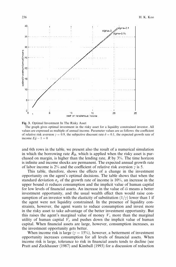
Fig. 3. Optimal Investment In The Risky AssetThe graph gives optimal investment in the risky asset for a liquidity constrained investor. All

values are expressed as multiple of annual income. Parameter values are as follows: the coe½cientof relative risk aversion g � 0:9, the subjective discount rate d � 0:1, the expected growth rate ofincome E ~gÿ 1 � 0

236 H. K. Koo

Ta

ble

II.

Th

eim

pli

cit

va

lue

of

hu

man

cap

ita

l,o

pti

mal

con

sum

pti

on

,an

do

pti

mal

inves

tmen

tin

the

risk

yass

et(p

erm

an

ent

inco

me

sho

cks,

in®

nit

eh

ori

zon

)

pa

ram

eter

va

lues

A Y�

0A Y�

1 4

A Y�

1 2

A Y�

1A Y�

2A Y�

5A Y�

10

A Y�

20

g�

5,

d�

0:1

p�

7:2

2p�

9:7

6p�

11:

2p�

13:

0p�

15:

4p�

19:

5p�

23:

5p�

28:

4o�

5c�

0:9

19

c�

1:0

0c�

1:0

5c�

1:1

1c�

1:2

2c�

1:4

5c�

1:7

6c�

2:3

0E

k~ g�

1:0

2p�

0:4

04

p�

1:1

8p�

1:6

3p�

2:3

8p�

3:4

2p�

5:5

5p�

8:1

3p�

12:

3s

g�

0:1

0�o�

5:0

0�

�o�

4:7

3�

�o�

3:5

9�

�o�

2:6

9�

�o�

1:9

2��o�

1:2

2��o�

0:8

8��o�

0:6

6�

g�

5,

d�

0:1

p�

9:3

4p�

10:

7p�

11:

5p�

12:

3p�

13:

3p�

15:

2p�

17:

4p�

20:

0o�

5c�

0:7

18

c�

0:7

52

c�

0:7

78

c�

0:8

18

c�

0:8

86

c�

1:0

7c�

1:3

4c�

1:8

3E

~ g�

1:0

2p�

1:4

1p�

2:4

8p�

3:1

9p�

3:5

6p�

4:0

4p�

5:2

3p�

7:1

5p�

10:

7s

g�

0:1

5�o�

5:0

0�

�o�

5:0

0�

�o�

4:4

2�

�o�

3:0

1�

�o�

1:9

1��o�

1:0

6��o�

0:7

4��o�

0:5

6�

g�

5,

d�

0:1

p�

8:8

3p�

10:

0p�

11:

0p�

12:

7p�

15:

2p�

19:

4p�

23:

5p�

28:

4o�

2c�

0:9

48

c�

0:9

97

c�

1:0

4c�

1:1

0c�

1:2

1c�

1:4

4c�

1:7

6c�

2:2

9E

~ g�

1:0

2p�

0:1

05

p�

0:5

07

p�

0:9

27

p�

1:7

9p�

3:3

3p�

5:4

7p�

8:0

4p�

12:

3s

g�

0:1

0�o�

2:0

0�

�o�

2:0

0�

�o�

2:0

0�

�o�

2:0

0�

�o�

1:8

6��o�

1:2

0��o�

0:8

7��o�

0:6

6�

g�

5,

d�

0:1

p�

9:5

8p�

10:

2p�

10:

9p�

11:

9p�

13:

2p�

15:

2p�

17:

4p�

20:

0o�

2c�

0:7

17

c�

0:7

42

c�

0:7

66

c�

0:8

10

c�

0:8

84

c�

1:0

7c�

1:3

4c�

1:8

3E

~ g�

1:0

2p�

0:5

66

p�

1:0

2p�

1:4

7p�

2:3

8p�

3:8

7p�

5:2

3p�

7:1

5p�

10:

5s

g�

0:1

5�o�

2:0

0�

�o�

2:0

0�

�o�

2:0

0�

�o�

2:0

0�

�o�

1:8

3��o�

1:0

6��o�

0:7

4��o�

0:5

5�

g�

5,

d�

0:1

p�

10:

0p�

11:

3p�

12:

1p�

13:

3p�

14:

8p�

18:

6p�

23:

0p�

28:

2o�

2c�

0:9

64

c�

1:0

1c�

1:0

4c�

1:1

0c�

1:1

9c�

1:4

2c�

1:7

4c�

2:2

8E

~ g�

1:0

2,

sg�

0:1

0p�

0:0

73

p�

0:4

81

p�

0:9

12

p�

1:4

3p�

1:8

2p�

4:5

8p�

7:8

7p�

12:

2R

B�

1:0

4,

R�

1:0

1�o�

2:0

0�

�o�

2:0

0�

�o�

2:0

0�

�o�

1:5

9�

�o�

1:0

0��o�

1:0

0��o�

0:8

5��o�

0:6

5�

g�

5,

d�

0:1

p�

9:8

1p�

10:

3p�

10:

7p�

11:

3p�

12:

5p�

15:

0p�

17:

3p�

20:

0o�

2c�

0:7

14

c�

0:7

35

c�

0:7

57

c�

0:7

96

c�

0:8

70

c�

1:0

6c�

1:3

4c�

1:8

3E

~ g�

1:0

2,

sg�

0:1

5p�

0:5

73

p�

1:0

3p�

1:4

9p�

1:6

6p�

2:1

3p�

4:9

4p�

7:0

5p�

1:0

55

RB�

1:0

4,

R�

1:0

1�o�

2:0

0�

�o�

2:0

0�

�o�

2:0

0�

�o�

1:3

8�

�o�

1:0

0��o�

1:0

0��o�

0:7

3��o�

0:5

5�


Ta

ble

II.

(co

nt.

)

g�

5,

d�

0:1

p�

11:

1p�

11:

7p�

12:

2p�

13:

1p�

14:

7p�

18:

6p�

23:

0p�

28:

2o�

1c�

0:9

77

c�

1:0

1c�

1:0

4c�

1:0

9c�

1:1

8c�

1:4

2c�

1:7

4c�

2:2

8E

~ g�

1:0

2p�

0:0

23

p�

0:2

40

p�

0:4

61

p�

0:9

10

p�

1:8

2p�

4:5

8p�

7:8

7p�

12:

2s

g�

0:1

0�o�

1:0

0�

�o�

1:0

0�

�o�

1:0

0�

�o�

1:0

0�

�o�

1:0

0��o�

1:0

0��o�

0:8

5��o�

0:6

5�

g�

5,

d�

0:1

p�

9:8

6p�

10:

2p�

10:

6p�

11:

3p�

12:

5p�

15:

0p�

17:

3p�

20:

0o�

1c�

0:7

14

c�

0:7

34

c�

0:7

55

c�

0:7

95

c�

0:8

70

c�

1:0

6c�

1:3

4c�

1:8

3E

~ g�

1:0

2p�

0:2

86

p�

0:5

16

p�

0:7

45

p�

1:2

0p�

2:1

3p�

4:9

4p�

7:0

5p�

10:

5s

g�

0:1

5�o�

1:0

0�

�o�

1:0

0�

�o�

1:0

0�

�o�

1:0

0�

�o�

1:0

0��o�

1:0

0��o�

0:7

3��o�

0:5

5�

238 H. K. Koo

in tolerance to risk when there is additional risk that is not insurable). There-fore, the wealth e¨ect dominates the substitution e¨ect for all levels of assets.

Table III: Table III shows the results of numerical simulations when the timehorizon is ®nite and income shocks are permanent. The expected annualgrowth rate of income is 2% and the coe½cient of relative risk aversion g is 5.It shows that given the same amount of ®nancial assets, as time to the ®naldate increases, the ratio of consumption to labor income declines, and theratio of investment in the risky asset to labor income increases. The longer thehorizon, the longer the time during which consumption needs to be ®nanced,and the smaller the ratio of optimal consumption to labor income. On theother hand, the longer the horizon, the longer the time over which the agentreceives labor income, and therefore, the higher the implicit value of humancapital, and the higher the investment in the risky asset.

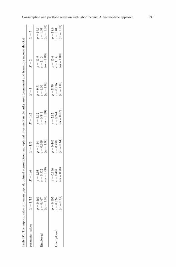
Table IV: In Table IV, we report simulation results for the case where incomeshocks have both permanent and transitory components. We assume thatlabor income follows the process in equation (11). We assume that st can taketwo values, 1 and 0. When st � 1, the agent is employed and his or her laborincome is equal to yt. When st � 0, the agent is unemployed and his or herlabor income is equal to 0. The time interval between two consecutive periodsis equal to one month and the probability of being employed in the next mothconditional on currently being employed is equal to 0.98 and the probability ofbeing employed in the next month conditional on currently being unemployedis equal to 0.5. The standard deviation of yt�1=yt is 10%. We assume that st�1

and yt�1=yt are independent. We also assume that g � 5 and d � 0:1.The value X denotes the ratio of ®nancial wealth to the annualized value of

y (i.e., twelve times the monthly value of y).The implicit value of human capital, p, and consumption, c, are given in the

unit of annualized y, i.e., p and c are the ratios of the implicit value of humancapital and annualized consumption (i.e., twelve times monthly consumption)to the annualized value of y, respectively. The table shows that the implicitvalue is increasing as ®nancial wealth increases, whether being employed ornot. Note that human capital is more valuable when the agent is employedthan when the agent is unemployed.

Consumption is low when ®nancial wealth is low, because the possibility ofbeing unemployed induces the agent to save a large amount. For the samelevel of ®nancial wealth, consumption is lower when the agent is unemployed,because the chance of being unemployed in the next month is larger.

The optimal portfolio selection shows an interesting pattern. When theagent is employed, the agent puts all the savings in the risky asset for allthe levels of ®nancial wealth shown in the table. However, when the agentis unemployed and ®nancial wealth is small, the agent puts less than the wholesavings in the risky asset, re¯ecting increased risk aversion in the face of atemporarily extreme situation.

5. Conclusion

This paper has investigated the consumption and portfolio selection problemof an agent who is constrained in ability to borrow against future labor


Ta

ble

III.

Th

eim

pli

cit

va

lue

of

hu

man

cap

ital,

op

tim

al

con

sum

pti

on

,an

do

pti

mal

inves

tmen

tin

the

risk

yass

et(p

erm

an

ent

inco

me

sho

cks,

®n

ite

ho

rizo

n)

pa

ram

eter

va

lues

A Y�

0A Y�

1 4

A Y�

1 2

A Y�

1A Y�

2A Y�

5A Y�

10

T�

10

p�

6:4

5p�

6:7

2p�

6:9

2p�

7:2

7p�

7:8

4p�

8:6

8p�

8:9

6g�

5,

d�

0:1

c�

0:9

88

c�

1:0

4c�

1:0

8c�

1:1

6c�

1:3

0c�

1:6

9c�

2:2

8o�

2p�

0:0

12

p�

0:2

13

p�

0:4

22

p�

0:8

45

p�

1:7

0p�

3:4

1p�

4:7

9E

~ g�

1:0

2,

sg�

0:1

0�o�

1:0

0��o�

1:0

0��o�

1:0

0��o�

1:0

0��o�

1:0

0��o�

0:7

9��o�

0:5

5�

T�

20

p�

9:0

7p�

9:5

0p�

9:8

3p�

10:4

p�

11:

5p�

13:

8p�

15:3

g�

5,

d�

0:1

c�

0:9

82

c�

1:0

2c�

1:0

5c�

1:1

1c�

1:2

2c�

1:5

0c�

1:9

1o�

2p�

0:0

18

p�

0:2

31

p�

0:4

50

p�

0:8

91

p�

1:7

8p�

4:4

5p�

6:5

5E

~ g�

1:0

2,

sg�

0:1

0�o�

1:0

0��o�

1:0

0��o�

1:0

0��o�

1:0

0��o�

1:0

0��o�

0:9

9��o�

0:7

2�

T�

30

p�

10:2

p�

10:

7p�

11:

1p�

11:9

p�

13:

2p�

16:

3p�

18:7

g�

5,

d�

0:1

c�

0:9

79

c�

1:0

1c�

1:0

4c�

1:1

0c�

1:2

0c�

1:4

5c�

1:8

1o�

2p�

0:0

21

p�

0:2

38

p�

0:4

59

p�

0:9

05

p�

1:8

0p�

4:5

5p�

7:3

6E

~ g�

1:0

2,

sg�

0:1

0�o�

1:0

0��o�

1:0

0��o�

1:0

0��o�

1:0

0��o�

1:0

0��o�

1:0

0��o�

0:8

0�

T�

10

p�

5:4

4p�

5:6

3p�

5:8

3p�

6:1

7p�

6:7

1p�

7:3

9p�

7:8

2g�

5,

d�

0:1

c�

0:8

70

c�

0:9

10

c�

0:9

51

c�

1:0

3c�

1:1

8c�

1:5

7c�

2:1

9o�

2p�

0:1

30

p�

0:3

40

p�

0:5

49

p�

0:9

69

p�

1:8

2p�

3:1

4p�

4:4

9E

~ g�

1:0

2,

sg�

0:1

5�o�

1:0

0��o�

1:0

0��o�

1:0

0��o�

1:0

0��o�

1:0

0��o�

0:7

1��o�

0:5

1�

T�

20

p�

7:4

1p�

7:7

0p�

7:9

9p�

8:5

2p�

9:4

0p�

10:

9p�

11:9

g�

5,

d�

0:1

c�

0:8

02

c�

0:8

31

c�

0:8

62

c�

0:9

20

c�

1:0

3c�

1:3

0c�

1:7

1o�

2p�

0:1

98

p�

0:4

19

p�

0:6

38

p�

1:0

8p�

1:9

7p�

4:0

9p�

5:7

6E

~ g�

1:0

2,

sg�

0:1

5�o�

1:0

0��o�

1:0

0��o�

1:0

0��o�

1:0

0��o�

1:0

0��o�

0:8

7��o�

0:6

2�

T�

30

p�

8:4

0p�

8:7

2p�

9:0

6p�

9:6

8p�

10:

7p�

12:6

p�

13:7

g�

5,

d�

0:1

c�

0:7

66

c�

0:7

92

c�

0:8

18

c�

0:8

69

c�

0:9

62

c�

1:2

0c�

1:5

4o�

2p�

0:2

34

p�

0:4

58

p�

0:6

82

p�

1:1

3p�

2:0

4p�

4:5

1p�

6:3

4E

~ g�

1:0

2,

sg�

0:1

5�o�

1:0

0��o�

1:0

0��o�

1:0

0��o�

1:0

0��o�

1:0

0��o�

0:9

4��o�

0:6

7�

240 H. K. Koo

Ta

ble

IV.

Th

eim

pli

cit

va

lue

of

hu

ma

nca

pit

al,

op

tim

al

con

sum

pti

on

,an

do

pti

mal

inves

tmen

tin

the

risk

yass

et(p

erm

an

ent

an

dtr

an

sito

ryin

com

esh

ock

s)

pa

ram

eter

va

lues

X�

1=1

2X�

1=6

X�

1=3

X�

1=2

X�

1X�

2X�

5

p�

0:4

66

p�

1:0

3p�

1:8

4p�

5:1

2p�

9:7

1p�

13:

9p�

19:1

Em

plo

yed

c�

0:4

67

c�

0:5

72

c�

0:6

59

c�

0:8

41

c�

1:0

0c�

1:1

5c�

1:4

0�o�

1:0

0��o�

1:0

0��o�

1:0

0�

�o�

1:0

0��o�

1:0

0�

�o�

1:0

0��o�

1:0

0�

p�

0:1

05

p�

0:1

96

p�

0:4

46

p�

2:8

2p�

8:7

9p�

13:

6p�

18:9

Un

emp

loy

edc�

0:3

24

c�

0:4

09

c�

0:4

98

c�

0:7

44

c�

0:9

76

c�

1:1

4c�

1:4

0�o�

0:8

7��o�

0:7

8��o�

0:6

4�

�o�

0:6

2��o�

1:0

0�

�o�

1:0

0��o�

1:0

0�


income. The paper has shown how the agent's implicit evaluation of humancapital changes when the value of asset holdings and labor income change.Namely, human capital is more valuable as the ratio of ®nancial assets toincome is larger (Proposition 2).

The paper has also presented numerical simulations. In particular, usingnumerical solutions the paper has shown that under the asumption that the®nancial market is perfect, investment in the risky asset is too high comparedto the real-world evidence (see Mehra and Prescott (1985)). The paper has alsoshown that the value of human capital is substantially lower when the agent isliquidity constrained than when the ®nancial market is perfect, and this lowvalue of human capital lowers optimal consumption and investment in therisky asset signi®cantly.

References

Campbell JY (1987) Does saving anticipate declining labor income? An altermative test of thepermanent income hypothesis. Econometrica 55:1249±1274

Cuoco D (1997) Optimal policies and equilibrium prices with portfolio constraints and stochasticincome. Journal of Economic Theory 12:33±73

Davis MHA, Norman AR (1990) Portfolio selection with transactions costs. Mathematics ofOperations Research 15:676±713

Deaton A (1991) Saving and liquidity constraints. Econometrica 59:1221±1248Deaton A, Laroque G (1992) On the behavior of commodity prics. Review of Financial Studies

59:1±23DreÁze JH, Modigliani F (1972) Consumption decisions under uncertainty. Journal of Economic

Theory 5:308±335Du½e D, Fleming W, Soner H, Zariphopoulou T (1997) Hedging in incomplete markets with

HARA utility. Journal of Economic Dynamics and Control 21:753±782Friedman M (1957) A theory of the consumption function. Princeton University Press, Princeton,

NJHall RE, Mishkin FS (1982) The sensitivity of consumption to transitory income: Estimates from

panel data on households. Econometrica 50:461±481He H, PageÁs HF (1993) Labor income, borrowing constraints, and equilibrium asset prices: A

duality approach. Economic Theory 3:663±696He H, Pearson ND (1991) Consumption and portfolio policies with incomplete markets and

short-sale constraints: The in®nite dimensional case. Journal of Economic Theory 54:259±304Karoui NE, Jeanblanc-PicueÂ M (1995) Optimization of consumption with labor income. mimeoKimball M (1990) Precautionary saving in the small and in the large. Econometrica 58:53±73Kimball M (1993) Standard risk aversion. Econometrica 51:589±613Koo HK (1992) Three essays on consumption and portfolio choice in the presence of market

frictions. unpublished dissertaion, Princeton UniversityKimball M (1998) Consumption and portfolio selection with labor income: A continuous-time

approach. Mathematical Finance 8:49±65MaCurdy TE (1982) The use of time series processes to model the error structure of earnings in an

longitudinal data analysis. Journal of Econometrics 18:83±134Mehra R, Prescott E (1985) The equity premium puzzle. Journal of Monetary Economics 15:145±

161Merton RC (1971) Optimum consumption and portfolio rules in a continuous-time model. Journal

of Economic Theory 3:373±413Merton RC (1991) Optimal investment strategies for university endowment funds. NBER Work-

ing Paper No. 3820Modigliani F, Brumberg RE (1954) Utility analysis and the consumption function. In: Kurihara

KK (ed.) Post-Keynesian economics, Rutgers University Press, New Brunswick, NJPratt JW, Zeckhauser RJ (1987) Proper risk aversion. Econometrica 55:143±154Skinner J (1988) Precautionary saving: A simulation study. Journal of Monetary Economics

22:237±255

242 H. K. Koo

Stiglitz JE, Weiss A (1981) Credit rationing in markets with imperfect information. AmericanEconomic Review 71:393±410

Svensson LEO, Werner I (1993) Nontraded assets in incomplete markets: Pricing and portfoliochoices. European Economic Review 37:1149±1168

Tauchen G, Hussey R (1991) Quadrature-based methods for obtaining approximate solutions tononlinear asset pricing models. Econometrica 59:371±396

Zeldes SP (1989a) Optimal consumption with stochastic income: Deviations from certaintyequivalence. Quarterly Journal of Economics 104:275±298

Zeldes SP (1989b) Consumption and liquidity constraints: An empirical investigation. Journal ofPolitical Economy 97:305±346


consumption and portfolio selection with labor income: a discrete-time approach

Documents