constraints on the prompt emission mechanism of gamma-ray
TRANSCRIPT
Constraints on the Prompt EmissionMechanism of Gamma-Ray Burstsusing Time-Resolved Spectroscopy
A dissertation submitted for the degree ofDoctor of Natural Sciences (Dr. rer. nat.)
by
Hoi-Fung Yu
to
Technische Universitat Munchen
and
Max-Planck-Institut fur extraterrestrische Physik
December 2015

Technische Universitat MunchenMax-Planck-Institut fur extraterrestrische Physik
Constraints on the Prompt EmissionMechanism of Gamma-Ray Bursts using
Time-Resolved Spectroscopy
Hoi-Fung Yu
Vollstandiger Abdruck der von der Fakultat fur Physik der Technischen Universitat Munchenzur Erlangung des akademischen Grades eines
Doktors der Naturwissenschaften
genehmigten Dissertation.
Vorsitzender: Univ.-Prof. Dr. Alejandro Ibarra
Prufer der Dissertation: 1. Priv.-Doz. Dr. Jochen Greiner2. Univ.-Prof. Dr. Elisa Resconi
Die Dissertation wurde am 03.12.2015 bei der Technischen Universitat Munchen eingereichtund durch die Fakultat fur Physik am 04.02.2016 angenommen.


To my beloved,
Pik-Ying Peggy Chan.
I

願聞顯據以窮理實浮詞虛貶竊非所懼
祖沖之《駁議》(462)
I will listen to the evidence,To pursue the truth.
Fancy words and false demeaning,Are not what I fear.
Zou Cung-Zi, Refutation (462)
For small creatures such as we the vastness is bearable only through love.
Carl Sagan, Contact (1985)
Tell your son to stop trying to fill your head with science - for to fill your heart with love isenough!
Richard Feynman, No Ordinary Genius: The Illustrated Richard Feynman (1996)
We are going to die, and that makes us the lucky ones. Most people are never going to diebecause they are never going to be born.
Richard Dawkins, Unweaving the Rainbow (1998)
我藏起來的秘密在每一天清晨裡暖成咖啡安靜的拿給妳
小柯〈不要說話〉陳奕迅《不想放手》(2008)
The secrets that I hide,In mornings of every day,
I warm and make them into coffee,Silently pass to you.
Little Or, Don’t TalkEason Chan, Don’t Wanna Let Go (2008)
II
Abstract
Since the birth of gamma-ray astronomy, large number of gamma-ray bursts (GRBs) has been
observed. These short, cosmological flashes of high-energy gamma-rays (∼ 1051 - 1053 erg s−1) are
believed to associate with exploding massive stars. Gamma-ray bursts can be used to probe the
physical and chemical environment of the early Universe at redshifts z > 10, thus the study of
GRBs is one of the most important in contemporary high-energy astrophysics. Through research
efforts in the past half century, large amount of high-quality gamma-ray data have been obtained.
However, a coherent understanding of the GRB prompt emission mechanism is still missing mainly
due to the difficulty in interpreting the data. In this dissertation, I study the emission mechanism
of the GRB prompt emission phase by time-resolved spectroscopy using the high-resolution data
obtained by the Fermi Gamma-ray Space Telescope Gamma-ray Burst Monitor (GBM). I present
detailed time-resolved spectral analysis of the brightest GBM GRBs. A novel quantity is invented
to measure the spectral sharpness which can be used to compare directly to theory. It is found that
the conventional explanation of the prompt emission phase by optically thin synchrotron emission
is inconsistent with a majority of observed spectra. Emission mechanism other than non-thermal
synchrotron radiation is likely required to achieve a full explanation of the GRB prompt emission
phase.
III
Zusammenfassung
Seit Beginn der Gammastrahlen-Astronomie wurde eine Vielzahl an Gammastrahlenblitzen (Gamma-
Ray Bursts, GRBs) beobachtet. Diese kurzlebigen, kosmologischen Strahlenblitze aus hochener-
getischen Gammastrahlen (∼ 1051 - 1053 erg s−1) werden im heutigen Verstandnis mit explodieren-
den massereichen Sternen in Verbindung gesetzt. Mithilfe von GRBs kann die physikalische und
chemische Umgebung des fruhen Universums bei Rotverschiebungen von z > 10 untersucht wer-
den, was die Erforschung von GRBs zu einer der wichtigsten Studien der heutigen Hochenergie-
Astrophysik macht. Durch die Forschung im letzten halben Jahrhundert wurde eine große Menge
an hochwertigen Messdaten im Bereich der Gammastrahlung gesammelt. Jedoch fehlt noch das
vollstandige Verstandnis der prompten Emission von GRBs , was hauptsachlich an der Schwierigkeit
beim Interpretieren der Messdaten liegt. In dieser Doktorarbeit untersuche ich den Emissions-
mechanismus der prompten Emissionsphase von GRBs durch zeitaufgeloste Spektroskopie anhand
der hochauflosenden Messdaten des Fermi Gamma-ray Space Telescope Gamma-ray Burst Mon-
itor (GBM). Ich prasentiere detailierte zeitaufgeloste Spektralanalysen der hellsten GBM GRBs.
Eine neue Große zum Messen der spektralen Scharfe, welche sich fur den direkten Vergleich mit
der Theorie eignet, wird eingefuhrt. Dabei ergibt sich, dass die konventionelle Erklarung der
prompten Emissionsphase durch optisch dunne Synchrotronstrahlung inkonsistent mit der Mehrheit
der beobachteten Spektren ist. Es werden wahrscheinlich andere Emissionsmechanismen als die
nichtthermische Synchrotronstrahlung benotigt, um eine vollstandige Erklarung fur die prompte
Emissionsphase von GRBs zu erhalten.
IV
Contents
Abstract III
Zusammenfassung IV
1 Gamma-Ray Bursts 1
1.1 A Brief History of GRB Research . . . . . . . . . . . . . . . . . . . . . . . . . . . . . 2
1.2 GRB Prompt Emission Models . . . . . . . . . . . . . . . . . . . . . . . . . . . . . . 7
1.2.1 Synchrotron Radiation . . . . . . . . . . . . . . . . . . . . . . . . . . . . . . . 8
1.2.2 Compton Scattering . . . . . . . . . . . . . . . . . . . . . . . . . . . . . . . . 13
1.2.3 Synchrotron Self-Compton . . . . . . . . . . . . . . . . . . . . . . . . . . . . . 15
1.3 Fermi Gamma-ray Burst Monitor . . . . . . . . . . . . . . . . . . . . . . . . . . . . . 17
1.4 Heuristic Fit Functions . . . . . . . . . . . . . . . . . . . . . . . . . . . . . . . . . . . 18
1.4.1 Band Function . . . . . . . . . . . . . . . . . . . . . . . . . . . . . . . . . . . 18
1.4.2 Smoothly Broken Power Law . . . . . . . . . . . . . . . . . . . . . . . . . . . 19
1.4.3 Cutoff Power Law . . . . . . . . . . . . . . . . . . . . . . . . . . . . . . . . . 20
1.4.4 Power Law . . . . . . . . . . . . . . . . . . . . . . . . . . . . . . . . . . . . . 20
1.4.5 Planck Function . . . . . . . . . . . . . . . . . . . . . . . . . . . . . . . . . . 20
1.4.6 Synchrotron Fit Function . . . . . . . . . . . . . . . . . . . . . . . . . . . . . 21
2 The Fermi GBM GRB Time-Resolved Spectral Catalog 22
2.1 Fermi GBM Data Reduction . . . . . . . . . . . . . . . . . . . . . . . . . . . . . . . 23
2.1.1 Detector Selection . . . . . . . . . . . . . . . . . . . . . . . . . . . . . . . . . 23
2.1.2 Data Type Selection . . . . . . . . . . . . . . . . . . . . . . . . . . . . . . . . 24
2.1.3 Energy Channel Selection and Background Fitting . . . . . . . . . . . . . . . 24
2.1.4 Burst and Spectrum Selection . . . . . . . . . . . . . . . . . . . . . . . . . . . 25
V
Contents VI
2.2 Spectral Analysis Method . . . . . . . . . . . . . . . . . . . . . . . . . . . . . . . . . 26
2.3 Time-Resolved Spectral Analysis Results . . . . . . . . . . . . . . . . . . . . . . . . . 27
2.3.1 General Statistics . . . . . . . . . . . . . . . . . . . . . . . . . . . . . . . . . . 27
2.3.2 Parameter-Parameter Scatter Plots . . . . . . . . . . . . . . . . . . . . . . . . 32
2.3.3 Parameter-Uncertainty Scatter Plots . . . . . . . . . . . . . . . . . . . . . . . 34
2.3.4 Ep Evolution . . . . . . . . . . . . . . . . . . . . . . . . . . . . . . . . . . . . 36
2.3.5 Search for Blackbodies . . . . . . . . . . . . . . . . . . . . . . . . . . . . . . . 41
2.4 Conclusions . . . . . . . . . . . . . . . . . . . . . . . . . . . . . . . . . . . . . . . . . 43
3 Synchrotron Cooling in Energetic Fermi GBM GRBs 45
3.1 Burst, Detector, and Data Selection . . . . . . . . . . . . . . . . . . . . . . . . . . . 46
3.2 Spectral Analysis Method . . . . . . . . . . . . . . . . . . . . . . . . . . . . . . . . . 47
3.3 Time-Resolved Spectral Analysis Results . . . . . . . . . . . . . . . . . . . . . . . . . 50
3.3.1 BAND Fits . . . . . . . . . . . . . . . . . . . . . . . . . . . . . . . . . . . . . 50
3.3.2 SYNC Fits . . . . . . . . . . . . . . . . . . . . . . . . . . . . . . . . . . . . . 52
3.4 Theoretical Implications . . . . . . . . . . . . . . . . . . . . . . . . . . . . . . . . . . 55
3.4.1 Hard-to-Soft Evolution and Intensity-Tracking Behavior . . . . . . . . . . . . 55
3.4.2 Synchrotron Emission and Band Function Fits . . . . . . . . . . . . . . . . . 56
3.4.3 Synchrotron Model Fits . . . . . . . . . . . . . . . . . . . . . . . . . . . . . . 58
3.4.4 Thermal Origin of Prompt Emission . . . . . . . . . . . . . . . . . . . . . . . 61
3.5 Conclusions . . . . . . . . . . . . . . . . . . . . . . . . . . . . . . . . . . . . . . . . . 61
4 The Sharpness of GRB Prompt Emission Spectra 63
4.1 Spectral Sharpness Analysis Method . . . . . . . . . . . . . . . . . . . . . . . . . . . 65
4.2 Spectral Sharpness Results . . . . . . . . . . . . . . . . . . . . . . . . . . . . . . . . 67
4.2.1 Spectral Evolution . . . . . . . . . . . . . . . . . . . . . . . . . . . . . . . . . 72
4.3 Consistency Checks . . . . . . . . . . . . . . . . . . . . . . . . . . . . . . . . . . . . . 75
4.3.1 Choices of Fit Models . . . . . . . . . . . . . . . . . . . . . . . . . . . . . . . 75
4.3.2 Choice of Data Domain . . . . . . . . . . . . . . . . . . . . . . . . . . . . . . 76
4.3.3 Choice of Triangle Domain . . . . . . . . . . . . . . . . . . . . . . . . . . . . 80
4.4 Theoretical Implications . . . . . . . . . . . . . . . . . . . . . . . . . . . . . . . . . . 81
4.5 Conclusions . . . . . . . . . . . . . . . . . . . . . . . . . . . . . . . . . . . . . . . . . 87
Contents VII
5 Summary and Future Directions 88
Bibliography 90
Acknowledgements 99
A Long Tables 102
Chapter 1
Gamma-Ray Bursts
“I can live with doubt, and uncertainty, and not
knowing. I think it is much more interesting to live
not knowing than have answers which might be
wrong. ... It doesn’t frighten me.”
- Richard Feynman
Gamma-ray bursts are among the most interesting and mysterious objects in the observable
Universe. Today, we know that they are cosmological transient gamma-ray sources isotropically
distributed across the sky, associated with exploding massive stars or compact object mergers.
However, we still do not know exactly what causes a GRB and how it emits the enormous energy
(typically ∼ 1053 erg within tens of seconds) that can outshine the total energy output in the entire
history of a galaxy.
An understanding of the emission mechanism of GRBs provides information of, for instance,
the dynamics of the relativistic outflows in the GRB jet, microphysics parameters in the emission
regions, structure and dynamics of the progenitor and the central engine (believed to be either a
black hole or a magnetar), chemical and physical properties of the circum-burst and interstellar
medium, host galaxy properties, and ultimately the evolution of the universe. The last item in the
list is one of the most important aspects of modern cosmology, which requires observational data
from high redshift sources.
Simply because they are extremely bright in the gamma-ray frequencies, GRBs easily hold the
record of the highest observed redshift among all kinds of cosmological sources known to date.
Moreover, the plausible linkage of GRBs to supernovae provides prospect of including GRBs into
the so-called cosmological ladder. Therefore, researches on the emission mechanism of the observed
1
Chapter 1. Gamma-Ray Bursts 2
gamma-rays from GRBs are of great importance and interest to not only high-energy astrophysi-
cists, but also to cosmologists and many scientists in the research fields of fundamental natural
science.
In this dissertation, I present my works as tiny contributions to the quest of revealing the true
GRB physics. Using the Fermi GBM data, I first performed time-resolved spectroscopy on a few
energetic GBM GRBs to investigate the emission mechanism of the prompt emission phase. In
Ch. 2, I present the first Fermi GBM GRB time-resolved spectral catalog (Yu et al. submitted).
In Ch. 3 (Yu et al. 2015a), we find that the conventional synchrotron emission models require
additional balckbodies or fine-tuned microphysics parameters to be able to get over the “line-of-
death” problem. In Ch. 4 (Yu et al. 2015b), we find that most of the spectra are indeed inconsistent
with a purely optically thin synchrotron emission model by a novel measured quantity. Before going
into the details of my researches, let’s do a revision on various emission mechanism models of GRBs.
Unless otherwise stated, in all following chapters, cgs units are used and errors are given at the
1σ confidence level.
1.1 A Brief History of GRB Research
The story begins 48 years ago.
For a long period of time, before the birth of high-energy astronomy, astronomers used to think
that the gamma-ray sky stays relatively constant except for statistical background fluctuations. In
the year of 1967, a group of satellites, named the Vela Satellite Network, were launched to identify
gamma-ray signatures emitted by nuclear weapons on Earth. The Vela satellites quickly detected
a number of mysterious gamma-ray flashes. Localization analysis results (Klebesadel et al. 1973)
showed that these gamma-rays are originated neither from the Earth nor the Sun, ruling out the
possibility of nuclear tests or solar origin. This new kind of extraterrestrial gamma-ray sources is
named gamma-ray bursts.
The Earth’s atmosphere has been protecting lifes on Earth from harmful gamma-rays for billions
of years. In order to study and understand these short (typically around tens of seconds) but lumi-
nous events, scientists have to launch detectors into space. Research progress has much advanced
when the Compton gamma-ray Observatory1 was launched in 1991, with the highly sensitive Burst
and Transient Source Explorer (BATSE) instrument (Fishman et al. 1989; Meegan et al. 1992)
1http://heasarc.gsfc.nasa.gov/docs/cgro/cossc/
Chapter 1. Gamma-Ray Bursts 3
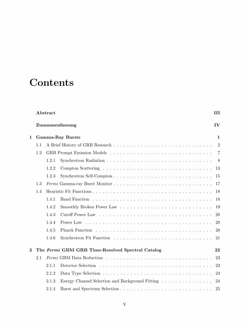
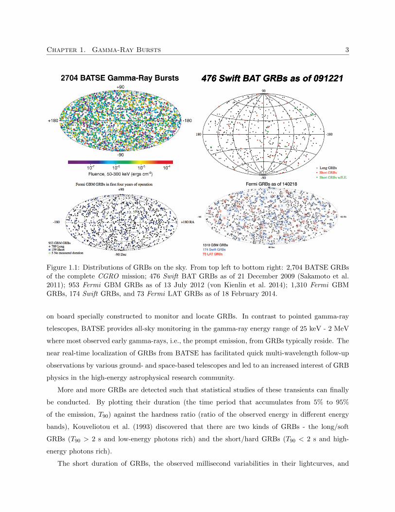
Figure 1.1: Distributions of GRBs on the sky. From top left to bottom right: 2,704 BATSE GRBsof the complete CGRO mission; 476 Swift BAT GRBs as of 21 December 2009 (Sakamoto et al.2011); 953 Fermi GBM GRBs as of 13 July 2012 (von Kienlin et al. 2014); 1,310 Fermi GBMGRBs, 174 Swift GRBs, and 73 Fermi LAT GRBs as of 18 February 2014.
on board specially constructed to monitor and locate GRBs. In contrast to pointed gamma-ray
telescopes, BATSE provides all-sky monitoring in the gamma-ray energy range of 25 keV - 2 MeV
where most observed early gamma-rays, i.e., the prompt emission, from GRBs typically reside. The
near real-time localization of GRBs from BATSE has facilitated quick multi-wavelength follow-up
observations by various ground- and space-based telescopes and led to an increased interest of GRB
physics in the high-energy astrophysical research community.
More and more GRBs are detected such that statistical studies of these transients can finally
be conducted. By plotting their duration (the time period that accumulates from 5% to 95%
of the emission, T90) against the hardness ratio (ratio of the observed energy in different energy
bands), Kouveliotou et al. (1993) discovered that there are two kinds of GRBs - the long/soft
GRBs (T90 > 2 s and low-energy photons rich) and the short/hard GRBs (T90 < 2 s and high-
energy photons rich).
The short duration of GRBs, the observed millisecond variabilities in their lightcurves, and
Chapter 1. Gamma-Ray Bursts 4
their high-energy gamma-ray emissions all suggest that the central engines of GRBs must be small
and compact. Therefore, astrophysicists first speculated that GRBs are originated from small scale
objects in the solar system or compact sources within our Milky Way Galaxy, e.g., galactic neutron
stars or black holes.
In contrast, BATSE data showed that GRBs are distributed isotropically across the sky (Briggs
et al. 1996; Hakkila et al. 1994; Tegmark et al. 1996). Figure 1.1 shows examples of GRB sky maps
taken from the CGRO,2 Swift, and Fermi mission.3 This discovery is a strong evidence against
theories of GRBs being originated from galactic sources or the supermassive black hole at the
galactic center, because we do not see GRBs on only the galactic plane. Therefore, despite the
non-detection of expected nuclear emission lines which prevented the measurement of cosmological
redshift, it is strongly suggested that GRBs are of extragalactic origins (e.g., van den Bergh 1983;
Paczynski 1986). This is later confirmed by Metzger et al. (1997) who reported the redshift of
GRB 970508 measured from its optical afterglow spectrum. Nowadays, it is believed that long
GRBs are results of gravitational collapse of massive stars (Woosley 1993, 1996; MacFadyen &
Woosley 1999), which is further supported by the discovery of GRB-Supernova connection (see,
e.g., Hjorth & Bloom 2012), while short GRBs are results of compact mergers, happened in distant
galaxies billions of years ago. Both scenarios result in a central black hole which powers the GRB
by accretion of surrounding matter (or a magnetar suggested by recent studies, see, e.g., Greiner
et al. 2015).
Since GRBs are confirmed to be cosmological sources, the emitting materials must be extremely
energetic and relativistic (GRB luminosities are typically 1051 - 1053 erg s−1). Astrophysicists
found the extreme energetics of GRBs puzzling - what kind of emission mechanism can produce
such powerful emissions that are still observable in the gamma-ray energy bands over a distance
of billions of light-years? One natural explanation is the so-called fireball model (Goodman 1986;
Meszaros et al. 1993; Meszaros & Rees 1993; Rees & Meszaros 1992, 1994; Tavani 1996; Piran
1999), in which the observed gamma-rays are emitted by outflow matter ejected from the central
engine. Since the prompt emission is observed in gamma-ray frequencies, the emitting matter
is beamed and extremely relativistic. If the outflow environment is optically thick, a thermal
spectrum due to photospheric radiation should result (Paczynski 1986). The thermal spectrum is
expected to be a blackbody, on top another non-thermal component (e.g., Ryde 2005). However,
spectral analysis showed little signs of blackbodies (e.g., Goodman 1986). Instead broken power-law
2http://heasarc.gsfc.nasa.gov/docs/cgro/batse/3http://fermi.gsfc.nasa.gov/ssc/observations/types/grbs/
Chapter 1. Gamma-Ray Bursts 5
shapes are found in the spectra of almost every GRB. Power laws are signatures of non-thermal
radiation processes, and the simplest among them is synchrotron radiation emitted by populations
of relativistic electrons gyrating around the local magnetic field (see, e.g., Rybicki & Lightman
1979).
Surprisingly, when the first BATSE GRB spectral catalog (Band et al. 1993; Ford et al. 1995;
Preece et al. 1996, 1998b) was published, about 30% of the time-resolved prompt emission spectra
are shown to be inconsistent with synchrotron emission models. This is the so-called synchrotron
“line-of-death” problem (Katz 1994a; Tavani 1995; Crider et al. 1998; Preece et al. 1998a, 2002).
Well, it is not a majority, maybe some minor modifications can be made to save the synchrotron
emission models, most people thought. The fact is that even after decades of research efforts, still
not a single synchrotron emission model can explain all these “outliners”.
In 2004 the Swift satellite4 was launched into orbit, on board which has a gamma-ray burst
dedicated instrument, the Burst Alert Telescope (BAT, Barthelmy 2000; Barthelmy et al. 2005),
used to monitor GRBs in a large field-of-view (2 steradians) in the 15 - 150 keV energy range.
When a GRB is detected, the BAT can request the spacecraft to slew towards the burst position
and conduct follow-up observations with the high precision X-Ray Telescope (XRT, Burrows et al.
2000; Hill et al. 2000) in the 0.3 - 10 keV energy range and the Ultraviolet/Optical Telescope
(UVOT). Swift has revolutionized afterglow studies, however BAT’s upper energy boundary is
usually below the peak energy in the prompt spectrum of a few hundred keV, it is difficult to draw
strong conclusion on the prompt emission mechanism using the Swift data alone.
Many afterglow (when the ejected shells collide with the interstellar medium and circum-burst
material blown away by the progenitor star) spectra are obtained by the BAT and XRT in X
rays, and also by many ground-based optical and radio telescopes thanks to the rapid and precise
localization of bursts by XRT circulated near real-time to the gamma-ray research community via
the Gamma-ray Coordinates Network5 (GCN). Sari et al. (1998) derived the expected spectral
behavior if the observed afterglow emission is emitted from shocked electrons via synchrotron
radiation (Paczynski & Rhoads 1993; Katz 1994b; Waxman 1997a,b; Wijers et al. 1997; Katz &
Piran 1997; Meszaros et al. 1998). The derived spectral slopes and evolutions of the spectral breaks
are compared to and agreed nicely with the observed afterglow spectra. It is very tempting to
explain the prompt emission and afterglow emission using the same radiation process, although a
fraction of the prompt emission spectra appear to be inconsistent with simple synchrotron theories.
4http://swift.gsfc.nasa.gov5http://gcn.gsfc.nasa.gov/gcn3_archive.html
Chapter 1. Gamma-Ray Bursts 6
The model to explain the prompt-afterglow emission, i.e., emission from colliding shells internal to
the jet of ejected matter vs. emission from collisions between shells and the external medium, is
known as the internal-external shock model.
Another very important GRB dedicated instrument is the Gamma-ray Burst Monitor (GBM,
Bissaldi et al. 2009; Meegan et al. 2009) on board the Fermi Gamma-ray Space Telescope6, which
was launched into orbit in 2008. The GBM provides all-sky monitoring and high temporal and
spectral resolution data of GRBs in the energy range of 8 keV - 40 MeV. It is complemented
by another instrument, the Large Area Telescope (LAT, Atwood et al. 2009), which covers more
energetic photons in the energy range of 20 MeV - 300 GeV. Its unprecedented wide energy coverage
has made Fermi an excellent telescope for studying the prompt emission properties of GRBs. The
data obtained by GBM have improved the understanding of GRBs by the research community in
recent years. For example, Burgess et al. (2011) fit a physical model to the GBM GRB data for the
first time, a big advancement to GRB spectral analysis since in the past only empirical fit functions
were used. It was found that a physical model with a synchrotron and a thermal component can
fit a few bright bursts adequately (Burgess et al. 2011, 2014a).
Multi-mission and multi-wavelength observations are hot topics for GRB studies. For example,
many gamma-ray satellites joined together to form the Interplanetary Network7 (IPN). The local-
ization of gamma-ray sources is difficult due to low photon statistics, the uncertainty is usually
large (a few degrees or more, see Connaughton et al. 2015). If a gamma-ray source is observed
simultaneously by multiple telescopes, a much smaller error contour of the gamma-ray source posi-
tion on the sky can be obtained by overlapping the locations deduced by each instrument, which is
known as the method of triangulation. Multi-mission inter-calibration can also be done, providing
more precise and accurate gamma-ray energetics of the GRB.
Ground-based GRB dedicated instruments play an important role in multi-wavelength studies
of GRBs. For instance, the Gamma-Ray Burst Optical/Near-Infrared Detector (GROND, Greiner
et al. 2008) mounted on the MPG 2.2 m Telescope on the mountain of La Silla, Chile, can observe
GRB afterglow simultaneously in 7 frequency bands from optical to near-infrared. High-quality
optical and near-infrared multi-band photometry obtained by the GROND instrument can deter-
mine redshift and host galaxy properties (e.g., gas and dust extinction, metallicity, etc.) of GRBs.
The multi-band data obtained by GROND also makes broad band spectral energy distribution
(SED) possible, which is essential to distinguish different theories and scenarios of the prompt and
6http://fermi.gsfc.nasa.gov7http://ipnpr.jpl.nasa.gov/index.cfm
Chapter 1. Gamma-Ray Bursts 7
afterglow emission mechanism. Although it was suggested that the optical emission during the
prompt emission period might not be related to the gamma-ray emission (e.g., Akerlof et al. 2000),
some recent simultaneous GROND and gamma-ray observations during the prompt phase did show
similarities (e.g., Elliott et al. 2014; Greiner et al. 2014).
Despite these progresses, more conundrums have also been found. Photons of GeV energies
have been observed in the LAT data (e.g., Axelsson et al. 2012), usually delayed relative to the keV
emission. Several empirical relations between the spectral parameters and the GRB’s energetics
are observed (e.g., Amati et al. 2002, 2008; Amati 2010; Ghirlanda et al. 2010; Yonetoku et al.
2004), but physical explanations are still lacking. Bursts with redshifts z > 9 are found (see, e.g.,
Tanvir 2013). Numbers of observed dark bursts (GRBs without afterglow emission, see, e.g., Fynbo
et al. 2001; Lazzati et al. 2002; Greiner et al. 2011) and orphan afterglows (GRBs without prompt
emission, see, e.g., Rhoads 1997; Huang et al. 2002; Cenko et al. 2013) are increasing. Delayed
X-ray flares and optical flares in the afterglow light curves are similar to the gamma-ray pulses in
the prompt lightcurves (e.g., Racusin et al. 2008; Ackermann et al. 2014; Elliott et al. 2014; Greiner
et al. 2014), suggesting plausible connection between the two emission phases. Extended emission
in GeV has been observed, in which the temporal property might indicate a separate emission
region (e.g., Abdo et al. 2010). Most interestingly, a third kind of GRBs are proposed (Gendre
et al. 2013; Stratta et al. 2013; Levan et al. 2014; Greiner et al. 2014, 2015) - ultra-long GRBs which
the prompt emission phase can last for hours or longer. Connection between ultra-long GRBs and
super-luminous supernovae suggests that the central engines of GRBs may not be black holes, but
highly magnetized neutron stars called magnetars (Greiner et al. 2015).
1.2 GRB Prompt Emission Models
In the fireball model, when the matter in the accretion disk around the central black hole is being
accreted inwards, a bipolar jet structure is formed because of angular momentum conservation.
Inside the jet there are shells of materials traveling outwards at relativistic speeds. When a faster
shell catches up and collides with a slower shell, shock waves will be formed which transform internal
energy of the bulk of ejected materials to the kinetic energy of electrons. Since electrons are much
easier to accelerate than baryons, it is generally believed that the prompt emission of GRBs is due
to leptonic process(es). In this section, I review some of these processes.
Chapter 1. Gamma-Ray Bursts 8
1.2.1 Synchrotron Radiation
Consider a single electron (e.g., Dermer & Menon 2009). If a magnetic field is present, the electron
experiences a Lorentz force
~F =d
dt(γme~v) = qe
(~E +
1
c~v × ~B
), (1.1)
where qe is the electron charge, me the electron rest mass, γ = 1/√
1− β the Lorentz factor, ~v = ~βc
the velocity, c the speed of light, ~E the electric field, and ~B the magnetic field.
Assuming the net electric field is negligible, there is no work done on the electron. Therefore,
we have the equations of motion in the direction parallel and perpendicular to the magnetic field
asd~v‖
dt= 0 ,
d~v⊥dt
=qe
γmec~v⊥ × ~B . (1.2)
Since γ is constant, v is constant. According to Eqn. (1.2), v‖ is constant and thus v⊥ is also
constant. Therefore, the electron accelerates only in the direction normal to ~v⊥ and ~B. Thus, the
motion is a combination of uniform linear motion and uniform circular motion, which is a helical
motion along ~B.
We can define the angular frequency of the motion
ωL =qeB
γmec, (1.3)
which is known as the Larmor frequency. The Larmor radius of gyration is thus
rL =v⊥ωL
=β⊥γmec
2
qeB. (1.4)
We can compute the synchrotron power radiated by the electron
P =2q4
eB2γ2β2
⊥3m2
ec3
. (1.5)
The average power can be found by averaging the pitch angle α between the velocity β = β⊥/ sinα
and the magnetic field. Since
〈β2⊥〉 =
β2
4π
∫sin2 α dΩ =
2β2
3, (1.6)
Chapter 1. Gamma-Ray Bursts 9
we have the average synchrotron radiation power formula
〈P 〉 =4
3σTcβ
2γ2UB . (1.7)
Here σT = 8πq4e/3m
2ec
4 is the Thomson cross section and UB = B2/8π is the magnetic energy
density.
It is interesting to compute the synchrotron spectrum. Because of the relativistic beaming effect,
the radiation received by the observer will appear to be concentrated in a cone (with opening angle
∼ 1/γ) about the electron velocity ~v from a small arc of each gyration. We also know that the
variation in the electric field of the observed beaming radiation depends only on γθ, where θ is the
polar angle about ~v. From geometry and the Larmor formulae, it can be shown that
γθ ≈ 2γ3ωLt sinα , (1.8)
and the observed pulse width
∆T ≈ 1
γ3ωL sinα. (1.9)
By Fourier transformation of the electric field we can obtain the power spectrum which is expected
to extend orders above the characteristic frequency
ωc ≡3
2γ3ωL sinα . (1.10)
So we have the electric field
E(ω) ∝∫ ∞−∞
f(ωct)eiωtdt ∝
∫ ∞−∞
f(ξ)eiωξ/ωcdξ . (1.11)
The latter proportionality by changing variable ξ = ωct.
Since the power is proportional to |E(ω)|2, from Eqn. (1.11) it must be of the form
P (ω) = CF(ω
ωc
). (1.12)
Here F is a dimensionless function and C is a constant of proportionality which carries all the
Chapter 1. Gamma-Ray Bursts 10
physical dimensions. Here, we just quote the standard textbook result (Rybicki & Lightman 1979):
P (ω) =
√3
2π
q3eB sinα
mec2F(ω
ωc
), (1.13)
where
F(x) = x
∫ ∞x
K5/3(ε)dε (1.14)
is known as the synchrotron kernel. Here K5/3 is the modified Bessel function of fractional order
5/3.
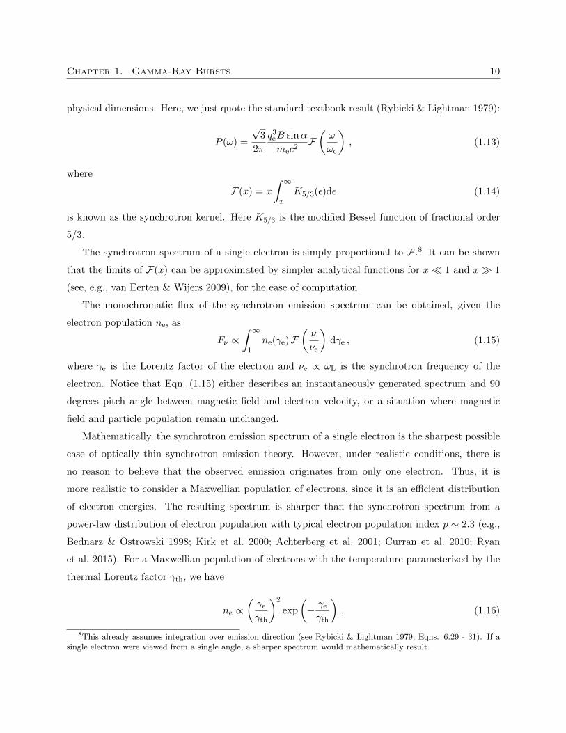
The synchrotron spectrum of a single electron is simply proportional to F .8 It can be shown
that the limits of F(x) can be approximated by simpler analytical functions for x 1 and x 1
(see, e.g., van Eerten & Wijers 2009), for the ease of computation.
The monochromatic flux of the synchrotron emission spectrum can be obtained, given the
electron population ne, as
Fν ∝∫ ∞
1ne(γe)F
(ν
νe
)dγe , (1.15)
where γe is the Lorentz factor of the electron and νe ∝ ωL is the synchrotron frequency of the
electron. Notice that Eqn. (1.15) either describes an instantaneously generated spectrum and 90
degrees pitch angle between magnetic field and electron velocity, or a situation where magnetic
field and particle population remain unchanged.
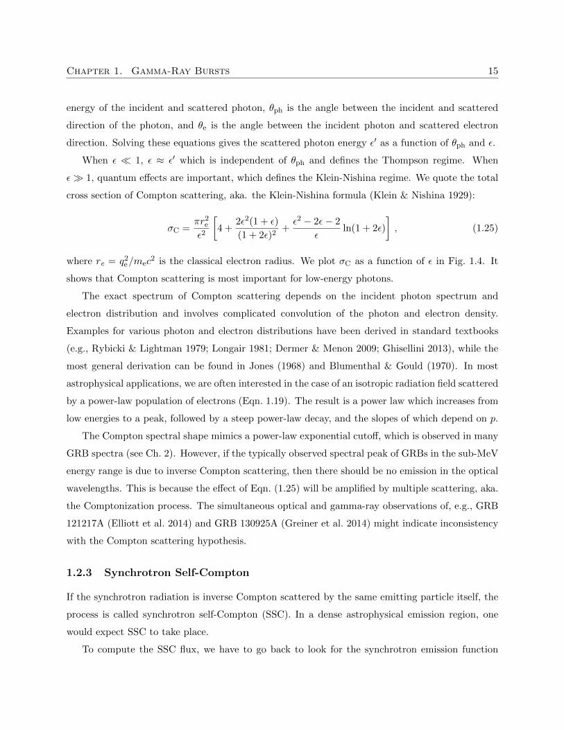
Mathematically, the synchrotron emission spectrum of a single electron is the sharpest possible
case of optically thin synchrotron emission theory. However, under realistic conditions, there is
no reason to believe that the observed emission originates from only one electron. Thus, it is
more realistic to consider a Maxwellian population of electrons, since it is an efficient distribution
of electron energies. The resulting spectrum is sharper than the synchrotron spectrum from a
power-law distribution of electron population with typical electron population index p ∼ 2.3 (e.g.,
Bednarz & Ostrowski 1998; Kirk et al. 2000; Achterberg et al. 2001; Curran et al. 2010; Ryan
et al. 2015). For a Maxwellian population of electrons with the temperature parameterized by the
thermal Lorentz factor γth, we have
ne ∝(γe
γth
)2
exp
(− γe
γth
), (1.16)
8This already assumes integration over emission direction (see Rybicki & Lightman 1979, Eqns. 6.29 - 31). If asingle electron were viewed from a single angle, a sharper spectrum would mathematically result.
Chapter 1. Gamma-Ray Bursts 11
10-1 100 101
Normalized Energy
10-1
100
Norm
aliz
ed E
nerg
y F
lux
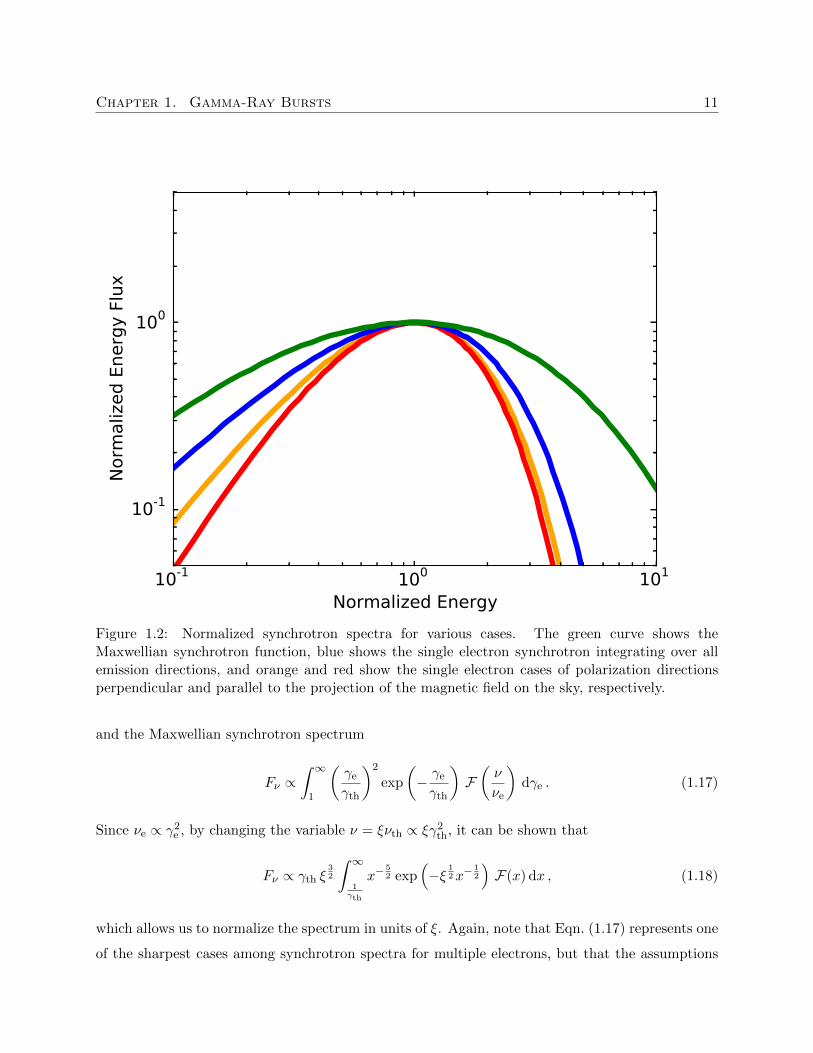
Figure 1.2: Normalized synchrotron spectra for various cases. The green curve shows theMaxwellian synchrotron function, blue shows the single electron synchrotron integrating over allemission directions, and orange and red show the single electron cases of polarization directionsperpendicular and parallel to the projection of the magnetic field on the sky, respectively.
and the Maxwellian synchrotron spectrum
Fν ∝∫ ∞
1
(γe
γth
)2
exp
(− γe
γth
)F(ν
νe
)dγe . (1.17)
Since νe ∝ γ2e , by changing the variable ν = ξνth ∝ ξγ2
th, it can be shown that
Fν ∝ γth ξ32
∫ ∞1γth
x−52 exp
(−ξ
12x−
12
)F(x) dx , (1.18)
which allows us to normalize the spectrum in units of ξ. Again, note that Eqn. (1.17) represents one
of the sharpest cases among synchrotron spectra for multiple electrons, but that the assumptions
Chapter 1. Gamma-Ray Bursts 12
of a single temperature and magnetic field are still unrealistic. The normalized νFν spectra of
the aforementioned synchrotron functions are ploted in Fig. 1.2. Observed emission will contain a
mixture of these and lead to smoother spectra.
Another reasonable assumption for the electron population is a power-law distribution of the
electron energies:
ne ∝ γ−pe : γe ≥ γmin , (1.19)
and the synchrotron spectrum with electron population index p is
Fν ∝∫ ∞γmin
γ−pe F(ν
νe
)dγe , (1.20)
where γmin is the minimum injection energy of the electron population. The Fν spectrum can be
solved as
Fν ∝ ν1−p
2
∫ ννmin
0
(ν
νe
) p−32
F(ν
νe
)d
(ν
νe
), (1.21)
where νmin is the minimum injection frequency of the electron population. As with temperature,
the observed spectrum will be smoother due to a mixture of νmin values in the emission. If we
substitute the approximation of F(x) ∼ x1/3 for x 1, we can recover the famous 1/3 low-energy
spectral slope below νmin for any value of p.
In reality, electron cooling should exist, as more energetic electrons lose their energy faster due
to radiative losses and cool down. One could consider, in addition to the minimum injection energy
break νmin, the cooling break νcool.
The optically thin synchrotron shock model (SSM) predicts two different scenarios, namely
fast cooling and slow cooling (see, e.g., Sari et al. 1998; Preece et al. 2002), depending on the
injection and evolution of the relativistic electron population. Both of them consist of a lower
and a higher frequency break, fixed by the values of the cooling frequency νcool and the minimum
injection frequency νmin for the relativistic electrons. The electrons in the shock are accelerated
to a minimum energy γmin. Assuming a power-law behavior for the electron energy distribution
n(γe) ∝ γ−pe , where γe ≥ γmin, the emission spectrum also has a power-law shape. As long as
p > 2, the distribution is characterized by its lower cutoff at γmin, and the integrated energy of the
population does not diverge at high electron energies.
There is a critical energy γcool such that electrons with energies above γcool emit a significant
amount of their energy via synchrotron cooling. The values of γcool and γmin correspond to νcool
Chapter 1. Gamma-Ray Bursts 13
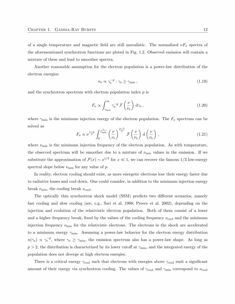
Figure 1.3: Schematic spectra for the SSM cooling scenarios. The left, middle, and right panelsshow the “slow”, “both”, and “fast” cases in the energy flux space. The shaded region representsthe possible location of νboth (i.e., Ep) when fitting the observed spectrum using a model withsmoothly jointed power laws. The photon distribution slopes are also indicated for each case.
and νmin, and the slow-cooling spectrum is given by
Fν,slow ∝
ν1/3 : νmin > ν ,
ν−(p−1)/2 : νcool > ν > νmin ,
ν−p/2 : ν > νcool ,
(1.22)
while the fast-cooling spectrum is given by
Fν,fast ∝
ν1/3 : νcool > ν ,
ν−1/2 : νmin > ν > νcool ,
ν−p/2 : ν > νmin .
(1.23)
Subtracting 1 from the spectral indices will give the power-law photon indices (i.e., α and β),
which lead to a synchrotron line-of-death α = −2/3 for both scenarios and a second line-of-death
α = −3/2 (Preece et al. 1998a) for the fast-cooling scenario. Figure 1.3 shows the schematic spectra
for the slow- and fast-cooling scenario, as well as the so-called “both” case where νcool/νmin (slow
cooling) or νmin/νcool (fast cooling) is close to unity. The both case can be considered to describe
an intermediate case of moderately fast cooling.
1.2.2 Compton Scattering
Compton scattering is one of the most important photon-particle interactions for high-energy as-
trophysics, because it describes the resulting photon spectrum when an external source of photons
scattered by a population of particles (electrons for most of the cases). Compton scattering is
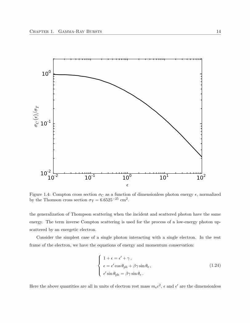
Chapter 1. Gamma-Ray Bursts 14
10-2 10-1 100 101 102
ε
10-2
10-1
100
σC
(ε)/σT
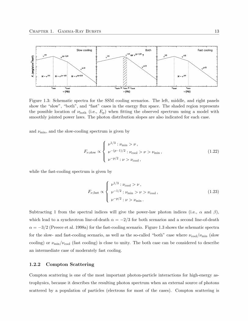
Figure 1.4: Compton cross section σC as a function of dimensionless photon energy ε, normalizedby the Thomson cross section σT = 6.6525−25 cm2.
the generalization of Thompson scattering when the incident and scattered photon have the same
energy. The term inverse Compton scattering is used for the process of a low-energy photon up-
scattered by an energetic electron.
Consider the simplest case of a single photon interacting with a single electron. In the rest
frame of the electron, we have the equations of energy and momentum conservation:
1 + ε = ε′ + γ ,
ε = ε′ cos θph + βγ sin θe ,
ε′ sin θph = βγ sin θe .
(1.24)
Here the above quantities are all in units of electron rest mass mec2, ε and ε′ are the dimensionless
Chapter 1. Gamma-Ray Bursts 15
energy of the incident and scattered photon, θph is the angle between the incident and scattered
direction of the photon, and θe is the angle between the incident photon and scattered electron
direction. Solving these equations gives the scattered photon energy ε′ as a function of θph and ε.
When ε 1, ε ≈ ε′ which is independent of θph and defines the Thompson regime. When
ε 1, quantum effects are important, which defines the Klein-Nishina regime. We quote the total
cross section of Compton scattering, aka. the Klein-Nishina formula (Klein & Nishina 1929):
σC =πr2
e
ε2
[4 +
2ε2(1 + ε)
(1 + 2ε)2+ε2 − 2ε− 2
εln(1 + 2ε)
], (1.25)
where re = q2e/mec
2 is the classical electron radius. We plot σC as a function of ε in Fig. 1.4. It
shows that Compton scattering is most important for low-energy photons.
The exact spectrum of Compton scattering depends on the incident photon spectrum and
electron distribution and involves complicated convolution of the photon and electron density.
Examples for various photon and electron distributions have been derived in standard textbooks
(e.g., Rybicki & Lightman 1979; Longair 1981; Dermer & Menon 2009; Ghisellini 2013), while the
most general derivation can be found in Jones (1968) and Blumenthal & Gould (1970). In most
astrophysical applications, we are often interested in the case of an isotropic radiation field scattered
by a power-law population of electrons (Eqn. 1.19). The result is a power law which increases from
low energies to a peak, followed by a steep power-law decay, and the slopes of which depend on p.
The Compton spectral shape mimics a power-law exponential cutoff, which is observed in many
GRB spectra (see Ch. 2). However, if the typically observed spectral peak of GRBs in the sub-MeV
energy range is due to inverse Compton scattering, then there should be no emission in the optical
wavelengths. This is because the effect of Eqn. (1.25) will be amplified by multiple scattering, aka.
the Comptonization process. The simultaneous optical and gamma-ray observations of, e.g., GRB
121217A (Elliott et al. 2014) and GRB 130925A (Greiner et al. 2014) might indicate inconsistency
with the Compton scattering hypothesis.
1.2.3 Synchrotron Self-Compton
If the synchrotron radiation is inverse Compton scattered by the same emitting particle itself, the
process is called synchrotron self-Compton (SSC). In a dense astrophysical emission region, one
would expect SSC to take place.
To compute the SSC flux, we have to go back to look for the synchrotron emission function
Chapter 1. Gamma-Ray Bursts 16
before averaging the emission direction. Crusius & Schlickeiser (1986) derived a general analytical
result for isotropic electron population in a randomly oriented magnetic field,
νF synν =
√3δ4
Dν′q3
eB
4πd2Lmec2
∫ ∞1
n′e(γ′)R(x)dγ′ , (1.26)
where δD = [γ(1− β cos θ)]−1 is the relativistic Doppler factor. All primed quantities are measured
in the comoving frame. The function
R(x) =x
2
∫ π
0
∫ ∞x/ sin θ
K5/3(ε)dεdθ (1.27)
can be approximated in the asymptotic limits as
R(x) =
3√2Γ2(1/3)
53√x : x 1 ,
π2 e−x (1− 99
162x
): x 1.
(1.28)
Here Γ is the gamma function and K5/3 is the Bessel function of fractional order 5/3.
The SSC flux is obtained by convolving the synchrotron flux with the Compton scattering
emission function. Finke et al. (2008) derived the form of the SSC flux in the observer frame as
νF SSCν =
9
16π
(1 + z)2σTν′2s
δ2Dc
2t2min
∫ ∞0
νF synν
ν ′3
∫ γ′max
γ′min
n′e(γ′)
γ′2FC(q,Γe)dγ
′dν ′ , (1.29)
where z is the redshift, σT = 8πr2e/3 is the Thomson cross section, tmin is the minimum variability
timescale, ν ′s is the frequency of the Compton scattered photon. The Compton scattering kernel
FC(q, Γe) is a function of photon and electron distribution. It is first derived by Jones (1968) and
then by Blumenthal & Gould (1970):
FC(q, Γe) =
[2q ln q + (1 + 2q)(1− q) +
1
2
Γ2eq
2(1− q)1 + Γeq
]H
(q;
1
4γ′2, 1
). (1.30)
Here, H(x; x1, x2) = 1 for x1 ≤ x ≤ x2 and H(x; x1, x2) = 0 elsewhere is the Heaviside function,
Γe = 4hν ′γ′ where h is the Planck constant, and
q =hν ′s/γ
′
Γe(1− hν ′s/γ′). (1.31)
The integration limits γ′max and γ′min can be obtained using the Heaviside function of q.
Chapter 1. Gamma-Ray Bursts 17
The SSC spectrum is predicted to be wider than the seed synchrotron spectrum (e.g., Ghisellini
2013). Thus it is believed that SSC cannot explain the observed GRB prompt emission spectra
(see, e.g., Baring & Braby 2004; Axelsson & Borgonovo 2015; Yu et al. 2015b).
A comprehensive review of GRB physics can be found in Piran (2004). Recent reviews on the
emission mechanism of GRBs can also be found in, e.g., Zhang (2014) and Pe’er (2015).
1.3 Fermi Gamma-ray Burst Monitor
The Fermi Gamma-ray Space Telescope, launched in June 2008, harbors two scientific instruments,
namely the Gamma-ray Burst Monitor (GBM, Meegan et al. 2009) and the Large Area Telescope
(LAT, Atwood et al. 2009). The GBM is a sensitive scintillation array covering the energy range
from 8 keV to 40 MeV, while the LAT is sensitive in the complementary energy range from 30 MeV
to 300 GeV. The GBM consists of twelve thallium activated sodium iodide (NaI(Tl), hereafter NaI)
detectors covering the energy range from 8 keV to 1 MeV and two bismuth germanate (BGO)
detectors covering the energy range from 200 keV to 40 MeV. This provides spectral coverage over
three orders of magnitude, which makes the GBM a powerful observing instrument for GRB prompt
emission.
The GBM observes the whole sky which is not occulted by the Earth (> 8 sr) and provides real-
time locations for GRB triggers. The arrangement of the NaI detectors allows GBM to locate GRBs
in a real-time manner; and the two BGO detectors are placed on opposite sides of the spacecraft
in order to cover all bursts coming from any direction in the sky. These real-time locations are
circulated via the Gamma-ray Coordination Network9 (GCN) which allows ground-based follow-up
observations. Occasionally, an Autonomous Repoint Request (ARR) can be accepted by the Flight
Software (FSW) which allows Fermi to slew towards the direction of the source, so that it can be
observed with the LAT.
The GBM generates three kinds of scientific data. The first type is CTIME which provides
coarse spectral resolution of 8 energy channels and fine temporal resolution of 0.256 s during the
nominal time period, i.e., before the trigger and 600 s after the trigger; during the trigger period,
the resolution is increased to 64 ms. The second type is CSPEC which provides coarse temporal
resolution at nominal (4.096 s) and trigger (1.024 s) period, and high spectral resolution of 128
pseudo-logarithmically scaled energy channels. The third type is time-tagged event (TTE) data
9http://gcn.gsfc.nasa.gov/gcn3_archive.html
Chapter 1. Gamma-Ray Bursts 18
which stores individual photon events tagged with arrival time (resolution of 2 µs), photon energy
channel (128 pseudo-logarithmic energy channels), and detector number (NaI 0 - 11 and BGO 0 -
1). TTE data were stored on board GBM in a recycling buffer. After 26 November 201210 this data
type became continuous. When GBM is triggered, the spacecraft will transmit pre- and post-trigger
TTE data (about 300 s in duration) to the ground as science data.
1.4 Heuristic Fit Functions
Conventionally, heuristic models are fit to the observed GRB prompt emission spectra. These
mathematical functions are empirical in origin. The most popular models are the Band function,
the smoothly broken power law, the cutoff power law, and the simple power law. The Planck
function (i.e., a blackbody) may be occasionally added to one of these models in some bursts (e.g.,
Meszaros et al. 2002; Ryde 2005; Guiriec et al. 2011; Axelsson et al. 2012; Guiriec et al. 2013;
Burgess et al. 2014a,b; Pe’er et al. 2015).
1.4.1 Band Function
The Band function (BAND) is a model in which a power law with high-energy exponential cutoff
and a high-energy power law are joined together by a smooth transition. It is an empirical function
proposed by Band et al. (1993), which fits most of the observed GRB spectra. Parametrized by
the peak energy Ep (despite the fact that there may not be a peak in the νFν space when the
high-energy photon index β ≥ −2) in the observed νFν spectrum, the photon model of BAND is
defined as
fBAND(E) = A
(
E100 keV
)αexp
[− (α+2)E
Ep
]: E < Ec ,(
E100 keV
)βexp (β − α)
(Ec
100 keV
)α−β: E ≥ Ec ,
(1.32)
where
Ec =
(α− βα+ 2
)Ep . (1.33)
In Eqns. (1.32) and (1.33), A is the normalization factor at 100 keV in units of ph s−1 cm−2 keV−1,
α is the low-energy power-law photon index, β is the high-energy power-law photon index, Ep is
the peak energy in the νFν space in units of keV, and Ec is the characteristic energy in units of
keV.
10http://fermi.gsfc.nasa.gov/ssc/data/access/gbm/
Chapter 1. Gamma-Ray Bursts 19
Note that the peak energy Ep represents the position of the peak in the model curve in the νFν
space, and the characteristic energy Ec represents the position where the low-energy power law with
an exponential cutoff ends and the pure high-energy power law starts. These two energies should be
distinguished from the break energy Eb which represents the position where the low-energy power
law joins the high-energy power law. Therefore, we should not compare the Band function’s Ep
or Ec to the smoothly broken power law’s Eb. We can compute the break energy where the two
power laws join together for the Band function. The derivation is already given by Kaneko et al.
(2006), here we only give the resulting equation:
Eb =
(α− βα+ 2
)Ep
2+
1
2Elb , (1.34)
in units of keV. Here Elb is the lower boundary of the detector. In the asymptotic limit, this term
vanishes and therefore Eb is proportional to Ep.
1.4.2 Smoothly Broken Power Law
The smoothly broken power law (SBPL) is a model of two power laws joined by a smooth transition.
It was first parameterized by Ryde (1999) and then re-parameterized by Kaneko et al. (2006):
fSBPL(E) = A
(E
100 keV
)b10(a−apiv) , (1.35)
where a = m∆ ln
(eq+e−q
2
), apiv = m∆ ln
(eqpiv+e
−qpiv
2
),
m = β−α2 , b = α+β
2 ,
q = log(E/Eb)2 , qpiv = log(100 keV/Eb)
2 .
(1.36)
In Eqns. (1.35) and (1.36), A is the normalization factor at 100 keV in units of ph s−1 cm−2 keV−1,
α and β are the low- and high-energy power-law photon indices respectively, Eb is the break energy
in units of keV, and ∆ is the break scale. Unlike the Band function, the break scale is not coupled
to the power-law indices, so SBPL is a five-parameters model if we let ∆ free to vary. In this
dissertation, we follow Kaneko et al. (2006), Goldstein et al. (2012), and Gruber et al. (2014) to fix
∆ = 0.3.
Chapter 1. Gamma-Ray Bursts 20
The peak energy of SBPL in the νFν space can be found at
Ep = 10xEb , x = ∆ tanh−1
(α+ β + 4
α− β
). (1.37)
Note that Eqn. (1.37) is only valid for α > −2 and β < −2.
1.4.3 Cutoff Power Law
The cutoff power law, aka. the Comptonized model (COMP), is a power-law model with a high-
energy exponential cutoff. Note that when β → −∞, BAND reduces to COMP:
fCOMP(E) = A
(E
100 keV
)αexp
[−(α+ 2)E
Ep
], (1.38)
where A is the normalization factor at 100 keV in units of ph s−1 cm−2 keV−1, α is the power-law
photon index, and Ep is the peak energy in the νFν space in units of keV.
1.4.4 Power Law
The power law (PL) is defined as
fPL(E) = A
(E
100 keV
)α, (1.39)
where A is the normalization factor at 100 keV in units of ph s−1 cm−2 keV−1, and α is the
power-law photon index.
1.4.5 Planck Function
The Planck function, aka. the blackbody model (BB), is defined as
fBB(E) = A
[(E/1 keV)2
exp(E/kT )− 1
], (1.40)
where A is the normalization factor at 1 keV in units of photons s−1 cm−2 keV−1 and kT is the
temperature of the blackbody in units of keV.
Chapter 1. Gamma-Ray Bursts 21
1.4.6 Synchrotron Fit Function
Empirical model fitting is the dominant technique for the past few decades of GRB spectroscopy
researches. One can obtain the best-fit parameter and then interpret the values by physics. How-
ever, the conventional models aforementioned have no direct connection to the physical processes
that they are trying to describe. In this work, a semi-empirical model is formulated to account for
the characteristic power-law indices for the two synchrotron cooling cases.
The synchrotron fit function (SYNC) is a modified triple power-law with sharp breaks defined
as
fSYNC(E) = A
(
E100 keV
)α: E < Eb,1,(
Eb,1
100 keV
)α−β (E
100 keV
)β: Eb,1 ≤ E < Eb,2,(
Eb,1
100 keV
)α−β ( Eb,2
100 keV
)β−γ (E
100 keV
)γ: E ≥ Eb,2 ,
(1.41)
where A is the normalization factor at 100 keV in units of photons s−1 cm−2 keV−1, α, β, and γ are
the power-law indices of the three segments (from low to high energy), and Eb,1 and Eb,2 are the
two break energies in units of keV. Here we fix α = −2/3 and β − γ = 1/2 to create a SYNC-slow
model for the slow-cooling scenario (Eq. 1.22). This makes it a four-parameter model with freely
varying A, Eb,1, Eb,2, and β (or equivalently, γ). We also fix α = −2/3 and β = −3/2 to create a
SYNC-fast model for the fast-cooling scenario (Eq. 1.23). This also makes a four-parameter model
with freely varying A, Eb,1, Eb,2, and γ.
Chapter 2
The Fermi GBM GRB
Time-Resolved Spectral Catalog
“[I do not] carry such information in my mind
since it is readily available in books. ... The value
of a college education is not the learning of many
facts but the training of the mind to think.”
- Albert Einstein
Gamma-ray bursts (GRBs) are the most energetic explosions known to humankind. Although
discovered in 1967 (Klebesadel et al. 1973) by the Vela Satellite Network, the physics of GRBs
still remains unsolved, e.g., the nature of the emission mechanism of the so-called prompt emission
phase. Today, we know that GRBs are gamma-ray emissions from cosmological sources (Metzger
et al. 1997) distributed isotropically across the sky (Meegan et al. 1992; Pendleton et al. 1994;
Briggs et al. 1996). The two kinds of GRBs, long/soft and short/hard (Kouveliotou et al. 1993),
are thought to have different origins. It is generally believed that long/soft (duration T90 > 2 s
and low-energy photon rich) GRBs are the result of gravitational collapse events from massive
progenitors, and short/hard (T90 < 2 s and high-energy photon rich) GRBs originate from compact
merger events.
A powerful method to discern the physical properties and emission mechanisms of GRBs is
through detailed spectral analysis. However, the spectral properties of individual GRB may be
significantly different. Therefore, analysis of large sample of burst spectra is necessary to obtain
a coherent physical picture. Such large spectral catalogs, some time-integrated and some time-
resolved, have been published for many hard X-ray or gamma-ray observing instruments, e.g., the
22
Chapter 2. The Fermi GBM GRB Time-Resolved Spectral Catalog 23
CGRO/BATSE (25 keV - 2 MeV, Pendleton et al. 1994; Preece et al. 2000; Kaneko et al. 2006;
Goldstein et al. 2013), BeppoSAX /GRBM (40 - 700 keV, Frontera et al. 2009), Swift/XRT (0.2 -
10 keV, Evans et al. 2009), Swift/BAT (15 - 150 keV, Sakamoto et al. 2008, 2011), Fermi/LAT
(20 MeV - 300 GeV, Ackermann et al. 2013), and Fermi/GBM (time-integrated, 8 keV - 40 MeV,
Nava et al. 2011; Goldstein et al. 2012; Gruber et al. 2014; von Kienlin et al. 2014).
This chapter presents the first Fermi GBM GRB time-resolved spectral catalog. In contrast to
previous time-resolved spectral catalogs of other instruments, the broad energy range covered by the
GBM allows a sensitive investigation at energies of a few hundred keV where the peaks or breaks
of the prompt emission spectra are located. This catalog presents time-resolved fit parameters
using standard fit functions, parameter-parameter and parameter-uncertainty correlations, spectral
evolutionary trends over time, in particular the peak energy Ep evolution, distributions of spectral
slopes (given in photon indices α and β), and plausible blackbody components. We present in Ch. 4
a novel measure of the sharpness of the spectral peak using this catalog burst sample (Yu et al.
2015b). The measure places a strong constraint on the physics of prompt emission models, ruling
out an optically thin synchrotron origin for the peak or break of the spectrum in a large majority
of cases.
This chapter is structured as follows. We describe the characteristics of GBM and the methods
of data selection and reduction in Sect. 2.1. The fitting models used in this catalog is described in
Sect. 1.4. The spectral analysis procedure is given in Sect. 2.2, and the fitting results are presented
in Section 2.3. We summarize our results and conclude in Sect. 2.4. Individual best-fit spectra are
tabulated in Appendix A.
2.1 Fermi GBM Data Reduction
2.1.1 Detector Selection
We apply the same detector selection criteria used in all official GBM GRB time-integrated spectral
catalogs (Goldstein et al. 2012; Gruber et al. 2014; von Kienlin et al. 2014). The detectors with
viewing angle larger than 60 degrees or blocked by the LAT or solar panels are removed (Bissaldi
et al. 2009; Goldstein et al. 2012; Gruber et al. 2014). For every spectrum, a maximum of three
NaIs with one BGO are used in the analysis. If more than three NaIs satisfied these criteria, the
NaIs with the smallest viewing angles are used in order to avoid binning bias towards the lower
energies (Goldstein et al. 2012).
Chapter 2. The Fermi GBM GRB Time-Resolved Spectral Catalog 24
2.1.2 Data Type Selection
There are three different types of data generated by GBM. The first type is CTIME which provides
coarse spectral resolution of 8 energy channels and fine temporal resolution of 0.256 s during the
nominal time period, i.e., before the trigger and 600 s after the trigger; during the trigger period,
the resolution is increased to 64 ms. The second type is CSPEC which provides coarse temporal
resolution at nominal (4.096 s) and trigger (1.024 s) period, and high spectral resolution of 128
pseudo-logarithmically scaled energy channels. The third type is time-tagged event (TTE) data
which stores individual photon events tagged with arrival time (resolution of 2 µs), photon energy
channel (128 pseudo-logarithmic energy channels), and detector number (NaI 0 - 11 and BGO 0 -
1). TTE data were stored on board GBM in a recycling buffer. After 26 November 20121 this data
type became continuous. When GBM is triggered, the spacecraft will transmit pre- and post-trigger
TTE data (about 300 s in duration) to the ground as science data. Therefore, for the 15 bursts
with evident precursor or emission longer than 300 s, we use the CSPEC data (about 8,000 s in
duration).
2.1.3 Energy Channel Selection and Background Fitting
To account for the poor transparency for gamma-rays of the silicone pad in front of the NaI crystal
and of the Multi Layer Insulation (MLI) around the detectors (Bissaldi et al. 2009), the energy
channels below 8 keV and the overflow channels above 900 keV are removed. A similar cutoff
criterion is also used in the BGOs so that only energy channels between 250 keV and 40 MeV are
used. An effective energy range from 8 keV to 40 MeV is used for the spectral analysis in this
chapter.
For each burst, a polynomial with order 2 - 4 is fit to every energy channel according to two
user-defined background intervals, before and after the emission period. The background model is
then interpolated across the emission period. This is done by varying the selected intervals and
order of polynomial until the χ2 statistics is minimised over all energy channels. The resulting
background intervals are then loaded to all detectors, generating the background model to be used
in the spectral analysis. The background intervals used in this catalog are identical to those used
in Gruber et al. (2014).
1http://fermi.gsfc.nasa.gov/ssc/data/access/gbm/
Chapter 2. The Fermi GBM GRB Time-Resolved Spectral Catalog 25
2.1.4 Burst and Spectrum Selection
We first select all the bursts detected by GBM in the first 4 years (i.e., from 14 July 2008 to 13
July 2012), which is the same GRB subset as used in the 4-yr GBM GRB time-integrated spectral
catalog (Gruber et al. 2014; von Kienlin et al. 2014). The GBM triggered on 954 GRBs in this period
of time (one of them triggered GBM twice, see von Kienlin et al. 2014). Time-resolved spectral
analysis requires bright bursts with sufficiently high signal-to-noise spectra. This bright subsample
is selected by applying the following criteria: 10 keV - 1 MeV energy fluence f > 4×10⁻⁵ erg cm−2
and/or 10 keV - 1 MeV peak photon flux Fp > 20 ph s−1 cm−2 (in either 64, 256, or 1,024 ms
binning timescales). These criteria are satisfied by 134 bursts out of the 954. Sixteen among them
are of the short burst class.
In order to alleviate the problem that the spectra from the brightest bursts dominate the
statistics, we further require each event to have at least 5 time bins in the light curves when binned
with signal-to-noise ratio (S/N) = 30. This optimal S/N is found by iterating the binning process
on characteristic bursts drawn from various fluence and peak-flux level, which does not significantly
merge peaks and valleys in the light curves while providing the highest number of time bins. As a
result, 81 bursts satisfy these criteria; among them there is only one short burst (GRB 120323A;
GBM trigger #120323507). In total, 1,802 time-resolved time bins and spectra were obtained.
Four different empirical models are fit to each spectrum, namely the Band function (BAND),
smoothly broken power law (SBPL), cutoff power law (COMP), and power law (PL). See Sect. 1.4
for function definitions. This results in a compilation of 1, 802× 4 = 7, 208 spectral fits. Compared
to the 4-yr GBM GRB time-integrated spectral catalog (Gruber et al. 2014; von Kienlin et al.
2014), the catalog presented here includes a lower number of GRBs (81 vs. 943), however, the
number of high-resolution spectra is higher (1,491, see Sect. 2.3, vs. 943).
For all the aforementioned mathematical functions, the resulting spectrum has a peak in the
νFν space if and only if α > −2 and β < −2. Since the Band function presumes α > β, for the
BAND fits with α ≤ −2, the spectrum decreases monotonically, and for those with β ≥ −2, the
spectrum increases monotonically. For the SBPL fits with α ≤ −2 or β ≥ −2, Ep is not calculated
because Eqn. (1.37) is invalid. Similarly, for the COMP fits with α ≤ −2, Ep is just a break and
the spectrum decreases monotonically, and obviously not there for the PL model.
Chapter 2. The Fermi GBM GRB Time-Resolved Spectral Catalog 26
2.2 Spectral Analysis Method
The light curves are binned according to the procedure described in Sect. 2.1, resulting in a total of
1,802 time bins and 1, 802× 4 = 7, 208 spectra. Time-resolved spectral analysis is performed using
the official GBM spectral analysis software RMFIT2 v4.3BA. RMFIT employs a modified forward-
folding technique based on the Levenberg-Marquardt algorithm. During the fitting process, the
fitting models are converted into counts. These counts are then compared to the observed counts
and RMFIT iterates itself until a best fit is found according to the chosen statistics for minimization.
In order to fold the model spectra into count space in the forward-folding process, detector
response matrices (DRMs) are generated using the GBM response matrices v2.0. These DRMs
contain information about the angular dependence of the detector efficiency, effective area of the
detectors, partial energy deposition, energy dispersion, nonlinearity in the detectors, and atmo-
spheric and spacecraft scattering of photons into the detectors. Therefore, they are functions of
photon energies, angular dependence between spacecraft and the source, and angle between space-
craft orientation relative to the Earth. In order to account for the orientation change of the detectors
relative to the burst direction because of the slew of the spacecraft, DRMs are generated for every
2 degrees on the sky and grouped into RSP2 files for each burst. This means each DRM is weighted
by the counts in the detectors for every 2 degrees of spacecraft slew.
The chosen statistics for minimization in the fitting process is the so-called Castor C-Statistics
(CSTAT). This is a modified statistical function based on the original Cash statistics (Cash 1979).
Since the background is Poissonian, the net count statistics is non-Gaussian, CSTAT is preferable
over the traditional χ2 statistics. However, CSTAT does not provide a goodness-of-fit measure as
χ2, because there is no standard probability distribution for the likelihood of CSTAT. As a result,
test statistics must be calculated and compared to the resulting CSTAT values by simulating the
fitting model a large number of times, which allows us to reject a model up to a certain confidence
level. Theoretically, this should be done for each burst separately, but due to the infeasibility of
generating large number of simulated spectra for all bursts, we adopt the values given in Gruber
et al. (2014) for models (8.58 for PL vs. COMP, and 11.83 for COMP vs. BAND or SBPL)
with various numbers of free parameters. These values, what we call the critical ∆CSTAT or
∆CSTATcrit, are listed in Table 1 of Gruber et al. (2014).
2The public version of the RMFIT software is available at http://fermi.gsfc.nasa.gov/ssc/data/analysis/
rmfit/
Chapter 2. The Fermi GBM GRB Time-Resolved Spectral Catalog 27
2.3 Time-Resolved Spectral Analysis Results
2.3.1 General Statistics
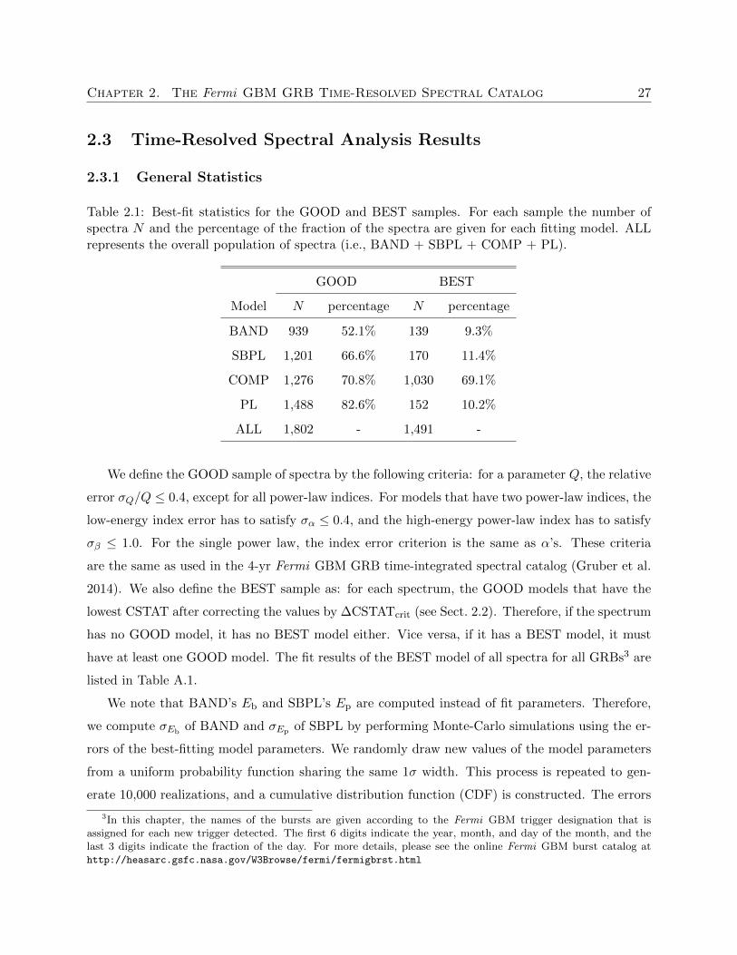
Table 2.1: Best-fit statistics for the GOOD and BEST samples. For each sample the number ofspectra N and the percentage of the fraction of the spectra are given for each fitting model. ALLrepresents the overall population of spectra (i.e., BAND + SBPL + COMP + PL).
GOOD BEST
Model N percentage N percentage
BAND 939 52.1% 139 9.3%
SBPL 1,201 66.6% 170 11.4%
COMP 1,276 70.8% 1,030 69.1%
PL 1,488 82.6% 152 10.2%
ALL 1,802 - 1,491 -
We define the GOOD sample of spectra by the following criteria: for a parameter Q, the relative
error σQ/Q ≤ 0.4, except for all power-law indices. For models that have two power-law indices, the
low-energy index error has to satisfy σα ≤ 0.4, and the high-energy power-law index has to satisfy
σβ ≤ 1.0. For the single power law, the index error criterion is the same as α’s. These criteria
are the same as used in the 4-yr Fermi GBM GRB time-integrated spectral catalog (Gruber et al.
2014). We also define the BEST sample as: for each spectrum, the GOOD models that have the
lowest CSTAT after correcting the values by ∆CSTATcrit (see Sect. 2.2). Therefore, if the spectrum
has no GOOD model, it has no BEST model either. Vice versa, if it has a BEST model, it must
have at least one GOOD model. The fit results of the BEST model of all spectra for all GRBs3 are
listed in Table A.1.
We note that BAND’s Eb and SBPL’s Ep are computed instead of fit parameters. Therefore,
we compute σEbof BAND and σEp of SBPL by performing Monte-Carlo simulations using the er-
rors of the best-fitting model parameters. We randomly draw new values of the model parameters
from a uniform probability function sharing the same 1σ width. This process is repeated to gen-
erate 10,000 realizations, and a cumulative distribution function (CDF) is constructed. The errors
3In this chapter, the names of the bursts are given according to the Fermi GBM trigger designation that isassigned for each new trigger detected. The first 6 digits indicate the year, month, and day of the month, and thelast 3 digits indicate the fraction of the day. For more details, please see the online Fermi GBM burst catalog athttp://heasarc.gsfc.nasa.gov/W3Browse/fermi/fermigbrst.html
Chapter 2. The Fermi GBM GRB Time-Resolved Spectral Catalog 28
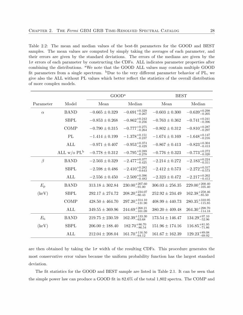
Table 2.2: The mean and median values of the best-fit parameters for the GOOD and BESTsamples. The mean values are computed by simply taking the averages of each parameter, andtheir errors are given by the standard deviations. The errors of the medians are given by the1σ errors of each parameter by constructing the CDFs. ALL indicates parameter properties aftercombining the distributions. aWe note that the GOOD ALL values may contain multiple GOODfit parameters from a single spectrum. bDue to the very different parameter behavior of PL, wegive also the ALL without PL values which better reflect the statistics of the overall distributionof more complex models.
GOODa BEST
Parameter Model Mean Median Mean Median
α BAND −0.665± 0.329 −0.691+0.329−0.267 −0.603± 0.300 −0.639+0.298
−0.205
SBPL −0.853± 0.268 −0.862+0.242−0.256 −0.763± 0.362 −0.741+0.241
−0.396
COMP −0.790± 0.315 −0.777+0.275−0.264 −0.802± 0.312 −0.810+0.287
−0.297
PL −1.414± 0.199 −1.378+0.151−0.237 −1.674± 0.169 −1.648+0.147
−0.216
ALL −0.971± 0.407 −0.953+0.374−0.429 −0.867± 0.413 −0.823+0.304
−0.413
ALL w/o PLb −0.778± 0.312 −0.795+0.289−0.278 −0.776± 0.323 −0.773+0.272
−0.320
β BAND −2.503± 0.329 −2.477+0.377−0.425 −2.214± 0.272 −2.183+0.224
−0.311
SBPL −2.598± 0.486 −2.410+0.282−0.643 −2.412± 0.573 −2.272+0.317
−0.573
ALL −2.556± 0.450 −2.509+0.396−0.482 −2.323± 0.472 −2.217+0.262
−0.412
Ep BAND 313.18± 302.84 230.00+207.60−91.00 306.03± 256.35 229.00+200.40
−105.40
(keV) SBPL 292.17± 274.72 208.20+234.07−80.43 252.92± 234.49 162.38+258.46
−85.50
COMP 428.50± 464.70 297.20+314.10−131.90 408.99± 440.73 280.35+310.95
−115.85
ALL 349.55± 369.96 244.69+268.21−101.09 380.20± 409.48 264.30+298.70
−114.18
Eb BAND 219.75± 230.59 162.39+133.30−63.68 173.54± 146.47 134.29+97.10
−52.96
(keV) SBPL 206.00± 188.40 182.70+86.70−86.54 151.96± 174.16 116.85+81.95
−71.86
ALL 212.04± 208.04 161.70+116.50−64.12 161.67± 162.39 129.23+89.08
−69.92
are then obtained by taking the 1σ width of the resulting CDFs. This procedure generates the
most conservative error values because the uniform probability function has the largest standard
deviation.
The fit statistics for the GOOD and BEST sample are listed in Table 2.1. It can be seen that
the simple power law can produce a GOOD fit in 82.6% of the total 1,802 spectra. The COMP and
Chapter 2. The Fermi GBM GRB Time-Resolved Spectral Catalog 29
SBPL can produce similar fractions of GOOD fits (70.8% and 66.6% respectively), and the BAND
can only produce a GOOD fit in around half of the sample spectra (52.1%). This indicates that
the conventional Band function may not be the optimal mathematical fit function for the majority
of time-resolved spectra (e.g., Giblin et al. 1999; Gonzalez et al. 2012; Sacahui et al. 2013).
Looking at the BEST sample, COMP has the largest fraction of BEST fits (69.1%), SBPL and
PL have 11.4% and 10.2% respectively, and BAND gives the lowest fraction, only 9.3%. However,
we note that these resulting statistics do not necessarily imply that the Comptonized model is
generally favored over the Band function. Kaneko et al. (2006) and Goldstein et al. (2012) showed
that there appeared to be a strong correlation between the S/N and the complexity of the BEST
model. Therefore, we cannot rule out the possibility that this observed preference is due to poor
count statistics at the high energies.
The mean and median values of the parameter distributions in the GOOD and BEST samples
are shown in Table 2.2. The “Mean” columns show the average value of each parameter distribution
and their errors are given by the standard deviations. The “Median” columns show the median
and 1σ errors of each parameter by constructing the CDFs. It can be seen that the mean and
median values of α and β agree well within the error bars, while those of Ep and Eb show only
marginal agreements within the error bars. The latter can be attributed to the log-normal, rather
then Gaussian, distribution of Ep and Eb, as shown in Figs. 2.1 and 2.2.
In Fig. 2.1 we show the distributions of the GOOD sample best-fit parameters. The top left
panel shows the GOOD distributions of the low-energy power-law index α. It can be seen that
there are two peaks in the ALL population. The peak at α ≈ −0.7 is due to the populations of
BAND, SBPL, and COMP collectively. The peak at α ≈ −1.4 is due to the population of PL alone.
The significantly softer values of PL’s α can also be seen in Table 2.2. Moreover, it is observed that
no GOOD value of PL’s α lies above α = −0.8.
The top right panel shows the GOOD distributions of the high-energy power-law index β. It
can be seen that both the BAND’s and SBPL’s β show very similar distributions, with a broad and
asymmetric peak of the populations at β ≈ −2.5. Only 7.6% of the overall population of β ≥ −2,
which implies that there is no peak in the νFν space and the spectrum increases monotonically,
therefore an extra break must exist above the GBM’s observing energy range.
The bottom left panel shows the GOOD distributions for the νFν peak energy Ep. We note
that Ep for SBPL is not a fit parameter but computed quantity by Eqn. (1.37). We also note that
the spectrum can increase or decrease monotonically if the conditions described in Sect. 2.1.4 are
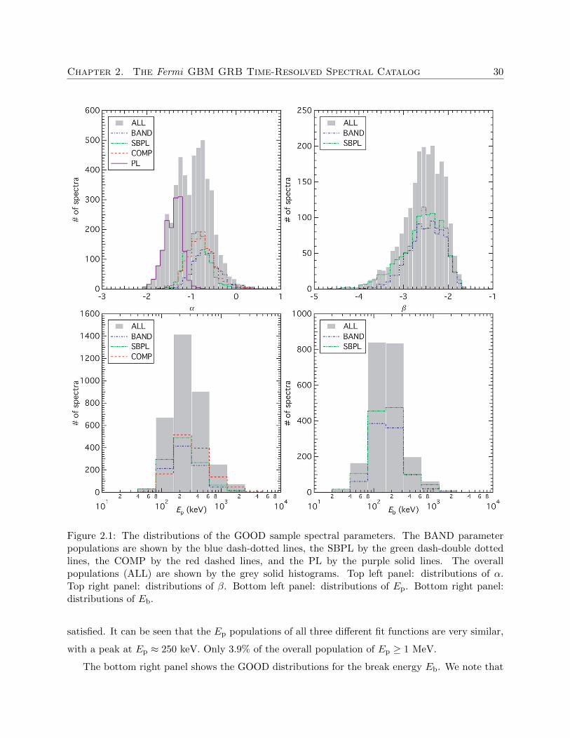
Chapter 2. The Fermi GBM GRB Time-Resolved Spectral Catalog 30
Figure 2.1: The distributions of the GOOD sample spectral parameters. The BAND parameterpopulations are shown by the blue dash-dotted lines, the SBPL by the green dash-double dottedlines, the COMP by the red dashed lines, and the PL by the purple solid lines. The overallpopulations (ALL) are shown by the grey solid histograms. Top left panel: distributions of α.Top right panel: distributions of β. Bottom left panel: distributions of Ep. Bottom right panel:distributions of Eb.
satisfied. It can be seen that the Ep populations of all three different fit functions are very similar,
with a peak at Ep ≈ 250 keV. Only 3.9% of the overall population of Ep ≥ 1 MeV.
The bottom right panel shows the GOOD distributions for the break energy Eb. We note that
Chapter 2. The Fermi GBM GRB Time-Resolved Spectral Catalog 31
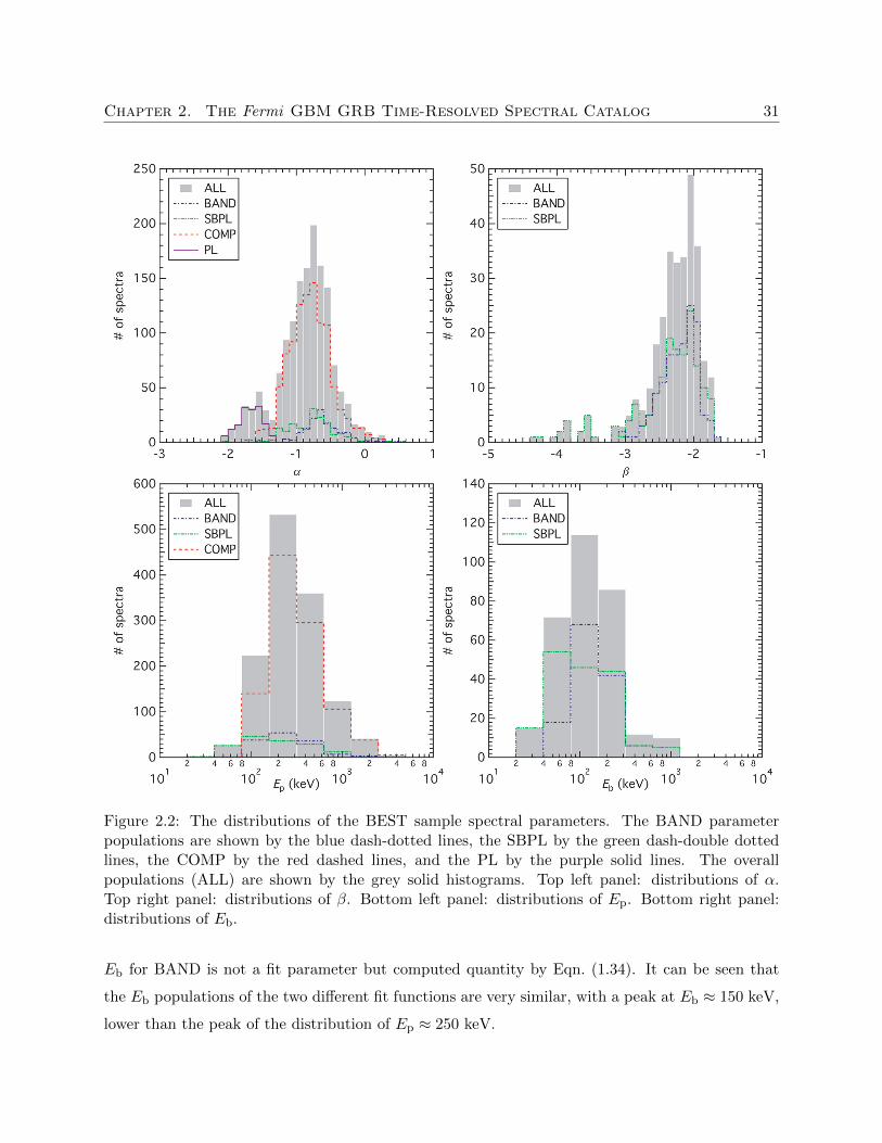
Figure 2.2: The distributions of the BEST sample spectral parameters. The BAND parameterpopulations are shown by the blue dash-dotted lines, the SBPL by the green dash-double dottedlines, the COMP by the red dashed lines, and the PL by the purple solid lines. The overallpopulations (ALL) are shown by the grey solid histograms. Top left panel: distributions of α.Top right panel: distributions of β. Bottom left panel: distributions of Ep. Bottom right panel:distributions of Eb.
Eb for BAND is not a fit parameter but computed quantity by Eqn. (1.34). It can be seen that
the Eb populations of the two different fit functions are very similar, with a peak at Eb ≈ 150 keV,
lower than the peak of the distribution of Ep ≈ 250 keV.
Chapter 2. The Fermi GBM GRB Time-Resolved Spectral Catalog 32
In Fig. 2.2 we show the distributions of the BEST sample best-fit parameters. The top left
panel shows the BEST distributions of the low-energy power-law index α. It can be seen that there
are two peaks in the ALL population, resulting from the two-peak distribution from the GOOD
distribution. The majority of the values of α for BAND, SBPL, and COMP are similar to that of
the GOOD distribution (≈ −2.5 up to −0.5). The peak at α ≈ −0.7, excluding those values from
PL, is dominated by the COMP model. It can be seen that the population of BAND’s α is slightly
harder that that of the SBPL’s which also shows a larger spread. The significantly softer values of
PL’s α in the BEST sample has a smaller spread than that in the GOOD sample, with no value lies
above α = −1.3. Therefore, the distinct behaviors of PL’s to the other fit function’s α is evident.
The top right panel shows the BEST distributions of the high-energy power-law index β. It can
be seen that the BAND’s β becomes more concentrated between −3.1 and −1.6, while the SBPL’s
β extend to much steeper values of about −4.4. The peak of the populations shifted to harder
values at β ≈ −2.1, comparing to the GOOD sample. As a result, 21% of the overall population of
β ≥ −2 (no peak in the νFν space).
The bottom left panel shows the BEST distributions for the νFν peak energy Ep. It can
be seen that the Ep population of COMP dominates the overall distribution, and that the COMP
population extends to higher energies (up to about 5 MeV) than the BAND and SBPL populations,
which instead extend to lower energies (down to about 20 keV). We do not find any spectrum with
very large Ep, with only 4.8% of the overall population of Ep ≥ 1 MeV.
The bottom right panel shows the distributions for the break energy Eb. It can be seen that
the Eb population of BAND has a clear peak at Eb ≈ 150 keV, while the Eb population of SBPL
has a broad peak (from 40 keV to 300 keV).
These general statistics suggests that when performing spectral analysis of GRBs, one should
not assume a Band spectrum (e.g., Giblin et al. 1999; Gonzalez et al. 2012; Sacahui et al. 2013).
Instead, one should always try different fit functions and compare the fit statistics to find the
best description to the data. Similar statistical behaviors are also observed in the time-integrated
spectral catalogs (Goldstein et al. 2012; Gruber et al. 2014).
2.3.2 Parameter-Parameter Scatter Plots
Figure 2.3 shows the scatter plots between the best-fit parameters of the BEST sample. The top
left panel shows the plot of β against α. Trends can neither be found between α and β for individual
models nor the overall population as a whole. It can be seen that SBPL’s β population extend to

Chapter 2. The Fermi GBM GRB Time-Resolved Spectral Catalog 33
Figure 2.3: The scatter plots between the BEST sample spectral parameters. The blue, red, andgreen data points represent BAND, COMP, and SBPL fits, respectively. Top left panel: β againstα. Top middle panel: Ep against α. Top right panel: Eb against α. Bottom left panel: Ep againstβ. Bottom right panel: Eb against β.
steeper values and have larger error bars in the same range of values of α. The larger error for
steeper β shows that the SBPL tends to mimic a COMP spectrum, in which β is poorly constrained
due to less photon statistics at the higher energies.
The top middle panel shows the plot of Ep against α. Trends can neither be found between α
and Ep for individual models nor the overall population as a whole. It can be seen that while the
data points seem to occupy the same region, SBPL’s Ep extends to lower energies and COMP’s Ep
extends to higher energies, for similar range of values for α.
The top right panel shows the plot of Eb against α. Similar to the plot of Ep, no trends can
be found for Eb, and SBPL’s Eb extends to lower energies for similar range of values of α. This is
because, according to Eqns. (1.34) and (1.37), Ep is proportional to Eb.
The bottom left panel shows the plot of Ep against β, and the bottom right panel shows the
Chapter 2. The Fermi GBM GRB Time-Resolved Spectral Catalog 34
plot of Eb against β. Since Ep is proportional to Eb, the two plots show similar behaviors. A slight
trend may exist between Ep against β in the population of BAND: steeper β tends to have lower
Ep. However, this trend is not seen in the population of SBPL.
These plots show that the SBPL produces larger uncertainties for steeper β, and has difficulties
to constrain the high-energy power-law behavior in comparison to the Band function.
2.3.3 Parameter-Uncertainty Scatter Plots
Figure 2.4 shows the scatter plots between the best-fit parameters and uncertainties of the param-
eters of the BEST sample. The top left panel shows the plot of σα against α. It is seen that the
SBPL gives the most scatter and large errors (extend to almost σα = 0.4), while other models give
relatively small errors of σα < 0.2. The PL gives the smallest σα ≤ 0.1. A clear trend for σα can
be seen: σα tends to be larger when α increases (i.e., becomes harder).
The top middle panel shows the plot of σβ against β. A clear trend is observed that σβ becomes
larger when β decreases (i.e., becomes softer/steeper). The trend is indeed expected because the
high-energy power-law slope becomes less constrained when the BAND or SBPL mimics a COMP
model, i.e., when there are less photon statistics at the high energies which leads to a cutoff behavior.
The top right panel shows the plot of σEp against Ep. It is observed that σEp of SBPL is
systematically larger than that of BAND and COMP for the same value of Ep. The values of σEp
for BAND and COMP also tend to lie above the dashed line, implying that σEp becomes larger
when Ep increases. We note that E ≈ 900 keV is the upper energy boundary of the NaIs, so that
there are only data contributed by the BGOs beyond this limit, providing less photon statistics
and thus increases the uncertainty in determining the spectral peak position.
The bottom left panel shows the plot of σEbagainst Eb. Comparing to the peak energies, σEb
of the break energies Eb have similar trends for both the BAND and SBPL fits. The errors lie
systematically above the dashed line for both models.
It is also of interest to investigate how the position of the spectral peak affects the uncertainties
in the spectral slopes. The bottom middle panel shows the plot of σα against Ep. A clear trend is
observed that the low-energy power-law slope becomes more uncertain when the spectrum peaks at
lower energies. This is because the low-energy spectral slope is determined by the photon statistics
below the peak energy. When the peak energy is smaller, there are relatively fewer data points to
constrain the value of the low-energy power-law slope. It is also observed that for the same value
of Ep, σα tends to be larger for the SBPL fits than that for the BAND or COMP fits.
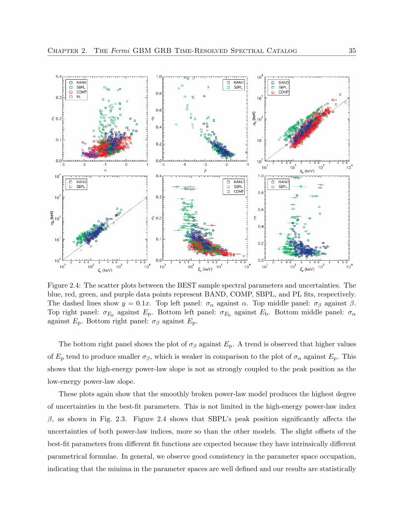
Chapter 2. The Fermi GBM GRB Time-Resolved Spectral Catalog 35
Figure 2.4: The scatter plots between the BEST sample spectral parameters and uncertainties. Theblue, red, green, and purple data points represent BAND, COMP, SBPL, and PL fits, respectively.The dashed lines show y = 0.1x. Top left panel: σα against α. Top middle panel: σβ against β.Top right panel: σEp against Ep. Bottom left panel: σEb
against Eb. Bottom middle panel: σαagainst Ep. Bottom right panel: σβ against Ep.
The bottom right panel shows the plot of σβ against Ep. A trend is observed that higher values
of Ep tend to produce smaller σβ, which is weaker in comparison to the plot of σα against Ep. This
shows that the high-energy power-law slope is not as strongly coupled to the peak position as the
low-energy power-law slope.
These plots again show that the smoothly broken power-law model produces the highest degree
of uncertainties in the best-fit parameters. This is not limited in the high-energy power-law index
β, as shown in Fig. 2.3. Figure 2.4 shows that SBPL’s peak position significantly affects the
uncertainties of both power-law indices, more so than the other models. The slight offsets of the
best-fit parameters from different fit functions are expected because they have intrinsically different
parametrical formulae. In general, we observe good consistency in the parameter space occupation,
indicating that the minima in the parameter spaces are well defined and our results are statistically
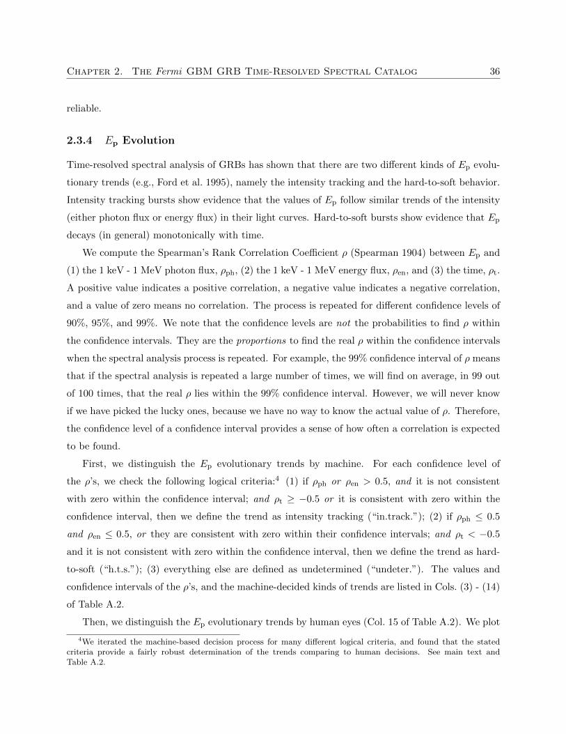
Chapter 2. The Fermi GBM GRB Time-Resolved Spectral Catalog 36
reliable.
2.3.4 Ep Evolution
Time-resolved spectral analysis of GRBs has shown that there are two different kinds of Ep evolu-
tionary trends (e.g., Ford et al. 1995), namely the intensity tracking and the hard-to-soft behavior.
Intensity tracking bursts show evidence that the values of Ep follow similar trends of the intensity
(either photon flux or energy flux) in their light curves. Hard-to-soft bursts show evidence that Ep
decays (in general) monotonically with time.
We compute the Spearman’s Rank Correlation Coefficient ρ (Spearman 1904) between Ep and
(1) the 1 keV - 1 MeV photon flux, ρph, (2) the 1 keV - 1 MeV energy flux, ρen, and (3) the time, ρt.
A positive value indicates a positive correlation, a negative value indicates a negative correlation,
and a value of zero means no correlation. The process is repeated for different confidence levels of
90%, 95%, and 99%. We note that the confidence levels are not the probabilities to find ρ within
the confidence intervals. They are the proportions to find the real ρ within the confidence intervals
when the spectral analysis process is repeated. For example, the 99% confidence interval of ρ means
that if the spectral analysis is repeated a large number of times, we will find on average, in 99 out
of 100 times, that the real ρ lies within the 99% confidence interval. However, we will never know
if we have picked the lucky ones, because we have no way to know the actual value of ρ. Therefore,
the confidence level of a confidence interval provides a sense of how often a correlation is expected
to be found.
First, we distinguish the Ep evolutionary trends by machine. For each confidence level of
the ρ’s, we check the following logical criteria:4 (1) if ρph or ρen > 0.5, and it is not consistent
with zero within the confidence interval; and ρt ≥ −0.5 or it is consistent with zero within the
confidence interval, then we define the trend as intensity tracking (“in.track.”); (2) if ρph ≤ 0.5
and ρen ≤ 0.5, or they are consistent with zero within their confidence intervals; and ρt < −0.5
and it is not consistent with zero within the confidence interval, then we define the trend as hard-
to-soft (“h.t.s.”); (3) everything else are defined as undetermined (“undeter.”). The values and
confidence intervals of the ρ’s, and the machine-decided kinds of trends are listed in Cols. (3) - (14)
of Table A.2.
Then, we distinguish the Ep evolutionary trends by human eyes (Col. 15 of Table A.2). We plot
4We iterated the machine-based decision process for many different logical criteria, and found that the statedcriteria provide a fairly robust determination of the trends comparing to human decisions. See main text andTable A.2.
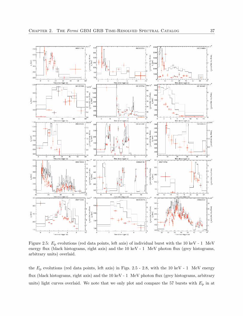
Chapter 2. The Fermi GBM GRB Time-Resolved Spectral Catalog 37
Figure 2.5: Ep evolutions (red data points, left axis) of individual burst with the 10 keV - 1 MeVenergy flux (black histograms, right axis) and the 10 keV - 1 MeV photon flux (grey histograms,arbitrary units) overlaid.
the Ep evolutions (red data points, left axis) in Figs. 2.5 - 2.8, with the 10 keV - 1 MeV energy
flux (black histograms, right axis) and the 10 keV - 1 MeV photon flux (grey histograms, arbitrary
units) light curves overlaid. We note that we only plot and compare the 57 bursts with Ep in at
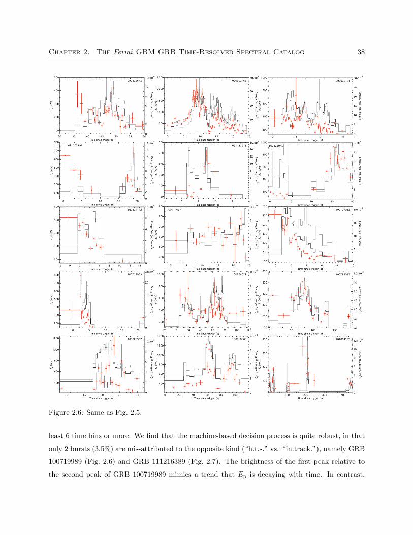
Chapter 2. The Fermi GBM GRB Time-Resolved Spectral Catalog 38
Figure 2.6: Same as Fig. 2.5.
least 6 time bins or more. We find that the machine-based decision process is quite robust, in that
only 2 bursts (3.5%) are mis-attributed to the opposite kind (“h.t.s.” vs. “in.track.”), namely GRB
100719989 (Fig. 2.6) and GRB 111216389 (Fig. 2.7). The brightness of the first peak relative to
the second peak of GRB 100719989 mimics a trend that Ep is decaying with time. In contrast,
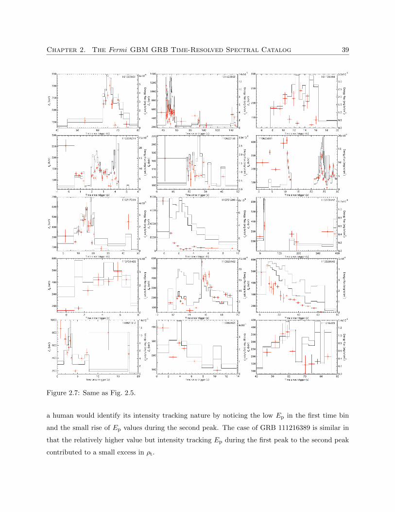
Chapter 2. The Fermi GBM GRB Time-Resolved Spectral Catalog 39
Figure 2.7: Same as Fig. 2.5.
a human would identify its intensity tracking nature by noticing the low Ep in the first time bin
and the small rise of Ep values during the second peak. The case of GRB 111216389 is similar in
that the relatively higher value but intensity tracking Ep during the first peak to the second peak
contributed to a small excess in ρt.
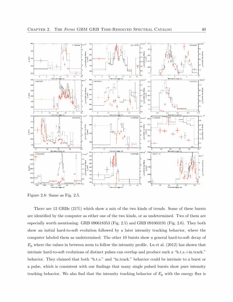
Chapter 2. The Fermi GBM GRB Time-Resolved Spectral Catalog 40
Figure 2.8: Same as Fig. 2.5.
There are 12 GRBs (21%) which show a mix of the two kinds of trends. Some of these bursts
are identified by the computer as either one of the two kinds, or as undetermined. Two of them are
especially worth mentioning: GRB 090618353 (Fig. 2.5) and GRB 091003191 (Fig. 2.6). They both
show an initial hard-to-soft evolution followed by a later intensity tracking behavior, where the
computer labeled them as undetermined. The other 10 bursts show a general hard-to-soft decay of
Ep where the values in between seem to follow the intensity profile. Lu et al. (2012) has shown that
intrinsic hard-to-soft evolutions of distinct pulses can overlap and produce such a “h.t.s.+in.track.”
behavior. They claimed that both “h.t.s.” and “in.track.” behavior could be intrinsic to a burst or
a pulse, which is consistent with our findings that many single pulsed bursts show pure intensity
tracking behavior. We also find that the intensity tracking behavior of Ep with the energy flux is
Chapter 2. The Fermi GBM GRB Time-Resolved Spectral Catalog 41
more prominent than that with the photon flux in all of the intensity tracking bursts.
A few more bursts are worth of mentioning. GRB 100707032 (Fig. 2.6), GRB 110721200, and
GRB 110920546 (both Fig. 2.7) are single pulsed, fast-rise-exponential-decay (FRED) bursts. All
of them show pure hard-to-soft behavior. Since the Ep evolutions and intensity profiles of these
FRED bursts are very similar, ρen and ρph ≈ −ρt & 0.5, thus the computer cannot determine their
evolutionary trends.
In short, we emphasize that even though the process of distinguishing “h.t.s.” and “in.track.”
bursts can be done automatically, the existence of “h.t.s.+in.track.” and FRED bursts can be
ambiguous to computers. We strongly encourage checking by human eyes after any automated
detection process of Ep evolutionary trends.
2.3.5 Search for Blackbodies
Many studies have reported evidence for thermal components with kT ∼ 10 keV in various GRBs
(e.g., Meszaros et al. 2002; Ryde 2005; Guiriec et al. 2011; Axelsson et al. 2012; Guiriec et al. 2013;
Burgess et al. 2014a,b; Pe’er et al. 2015). Therefore, adding a blackbody component (i.e., a Planck
function) to the fit function is a natural way to explore the data in this time-resolved spectral
catalog.
We find that except for the single power law, in most of the cases (& 90%) it is not possible
to obtain converged fits when the blackbody is added to other fitting models (i.e., BAND, COMP,
and SBPL). However, we note that the ability of a model to fit the data depends also on the count
statistics. Abdo et al. (2009) performed a joint GBM-LAT analysis to GRB 090902B (GBM trigger
#090902462, see discussion below) that they can fit a BAND plus PL model to the burst, which
is expected because there are more statistics to constrain more parameters. Our results in this
chapter indicates the difficulty of fitting a model with 5 or more parameters to the GBM data
alone using the S/N = 30 criterion.
The power law plus blackbody model (PLBB) is defined as (see Sect. 1.4)
fPLBB(E) = APL
(E
100 keV
)α+ABB
[(E/1 keV)2
exp(E/kT )− 1
], (2.1)
where APL and ABB are the normalization factors for the power-law and blackbody component,
respectively.
Since PLBB is a not a nested model, it is necessary to perform ∆CSTATcrit simulations for every
Chapter 2. The Fermi GBM GRB Time-Resolved Spectral Catalog 42
pair of competing models, instead of just counting the number of free parameters (see Gruber et al.
2014). However, doing a large number of simulations for every spectrum is obviously impractical.
We therefore first identify plausibly significant PLBB spectra by using the same ∆CSTATcrit criteria
for a 4-parameters model. Then we generate 10,000 realisations for the identified time intervals
for every burst in this subsample and obtain the ∆CSTATcrit for each burst. Then we compare
the ∆CSTAT between the BEST model and the PLBB model for each spectrum, i.e., ∆CSTAT =
CSTAT(BEST)− CSTAT(PLBB).
Table 2.3: The 4 bursts with N number of PLBB-identified spectra, and their respective critical∆CSTAT values.
GRB name N ∆CSTATcrit
090618353 2 19.55
090902462 32 32.75
110622158 2 12.32
110920546 6 148.37
As a matter of fact, 56 plausibly significant PLBB spectra are identified among 16 bursts, in
which 14 bursts have only 1 plausible spectrum identified. Since a blackbody component is likely to
be present in multiple spectra within a burst if it is real, we drop these 14 bursts and concentrate on
the remaining 4 bursts (42 spectra in total) with multiple PLBB-identified spectra. These bursts
are listed in Table 2.3, and their simulated ∆CSTATcrit values are also given.
We find that the spectra of the bursts listed in Table 2.3 have ∆CSTAT > ∆CSTATcrit, except
for GRB 110920546. These 36 PLBB spectral parameters are listed in Table A.3. We note that the
4 PLBB spectra from GRB 090618353 and GRB 110622158 have values of kT ∼ 20 keV, while the
32 spectra from GRB 090902B show kT ∼ 200 keV. In GRB 090902B, Abdo et al. (2009) identified
an extra power-law component on top of Band functions with hard values of Ep using wider time
bins and joint GBM-LAT data. Using only the GBM data, we find that most of the BAND plus PL
fits of our more resolved time bins in this time interval are either poorly constrained, unconstrained,
or even not converged; but, interestingly, our values of the PL indices are very similar to theirs
(α ≈ −1.8). This indicates the ability of a model to fit data depends on (1) how many free
parameters (in this case, BB vs. BAND), and (2) the count statistics (GBM alone vs. GBM-LAT).
We also note that Pe’er et al. (2012) used a thermal plus non-thermal theoretical model to apply
to the spectra of this burst, in which they claimed that the data are consistent with such a hybrid
Chapter 2. The Fermi GBM GRB Time-Resolved Spectral Catalog 43
emission model.
We note that the ∆CSTATcrit can vary much across different bursts. Recently, Burgess et al.
(2015) showed that it is very plausible to get false positive for an extra blackbody component in
time-integrated spectra due to severe spectral evolution. Therefore, we recommend researchers to
perform independent simulations on time-resolved spectra for different bursts in order to reduce
the chance of false positives.
2.4 Conclusions
We present the first official gamma-ray burst time-resolved spectral catalog of the brightest subset
of bursts observed by the Fermi GBM in its first 4 years of mission. We have obtained 1,491
spectra from 81 bursts with high spectral and temporal resolution. We observe a preference of the
Comptonized model (i.e., the high-energy cutoff power law) to fit 69% of our spectra sample the
best, under our chosen S/N = 30. However, we note that this may be due to poor count statistics
at the high energies, as previous catalogs have pointed out (see, e.g., Kaneko et al. 2006; Goldstein
et al. 2012). Similarly, Ackermann et al. (2012) showed that for the bursts observed in GBM which
happen to be in the field-of-view of the LAT but remain undetected, the upper limits are usually
inconsistent with the GBM fit Band function’s β, extrapolated to the LAT energy range. This
is consistent with the observed fact that COMP dominates the BEST sample, however there is a
caveat that the sample selected by Ackermann et al. (2012) may be intrinsically softer in nature.
We have not observed significant deviations of the distributions of fit parameters from those
observed in the Fermi GBM GRB time-integrated spectral catalogs. In the 4-yr GBM GRB time-
integrated spectral catalog (Gruber et al. 2014; von Kienlin et al. 2014), the question of whether
there is any time-resolved spectrum with very high value of Ep was raised. Down to the level of the
temporal resolution of the binned data sets in the current catalog, the answer is “no”. The largest
value of Ep found in this study is 7, 400 ± 600 keV, in GRB 110721A (GBM trigger #110721200,
from −1.024 to 0.711 s relative to GBM trigger time). The time-integrated Ep of this burst is
450 ± 30 keV (T90 = 21.822 s starting from 0.003 s after GBM trigger time, Gruber et al. 2014),
which is much lower and indicates severe spectral evolution. However, we note that very high
Ep on much shorter timescales cannot be excluded. Gruber et al. (2014) discussed the very high
Ep = 15 ± 2 MeV observed by Axelsson et al. (2012) in the “higher resolution” first time bin of
GRB 110721A. Our aforementioned Ep = 7, 400±600 keV is consistent at 2σ level with their “lower
Chapter 2. The Fermi GBM GRB Time-Resolved Spectral Catalog 44
resolution” first time bin of Ep = 5, 410+410−420 keV.
We establish possible logical criteria for automated process of distinguishing between “hard-to-
soft” and “intensity tracking” spectral evolutionary trends. With this selection scheme, only 3.5%
of bursts would be mis-attributed to the opposite kind. However, we note that inspections using
human eyes are often necessary because of the existence of “hard-to-soft + intensity tracking” and
FRED bursts.
We also search for plausible blackbody components in the time-resolved spectra by performing
simulations on individual bursts. We find that only 3 bursts show extra blackbodies in multiple
time bins. We also find that constrained fit results can be obtained only when the Planck function
is added to the simple power law, using S/N = 30 binning criterion and GBM data alone.
Finally, we note that the fact that very few blackbodies are found in this catalog does not
necessarily imply that thermal components are in general not a dominant component for the prompt
emission mechanism. There are many works recently showing that a thermal model can give rise
to the observed Band shape (e.g., Pe’er et al. 2006; Giannios 2008; Pe’er & Ryde 2011; Ryde et al.
2011; Vurm et al. 2011; Lazzati et al. 2013). Whether thermal or non-thermal emission dominates
the emission mechanism of GRB prompt spectra is a debated topic. Yu et al. (2015b) showed that
all standard optically thin synchrotron emission functions are just too smooth to explain the peaks
or breaks in the time-resolved spectra, and an independent conclusion is also drawn by Axelsson
& Borgonovo (2015) using peak-flux spectra from the GBM GRB time-integrated spectral catalog.
Recently, semi-empirical models (Ch. 3, Yu et al. 2015a) and physical models (e.g., Burgess et al.
2011, 2014a; Zhang et al. 2016) are fit to time-resolved spectra of a few GRBs. In the future, direct
fitting of serious theoretical models, as oppose to empirical models, is likely the key to resolve these
issues.
Chapter 3
Synchrotron Cooling in Energetic
Fermi GBM GRBs
“An expert is a person who has found out by his
own painful experience all the mistakes that one can
make in a very narrow field.”
- Niels Bohr
Gamma-ray bursts are the most luminous explosions in the Universe known to date. The first
GRB was discovered in 1967 (Klebesadel et al. 1973), and after over 45 years of research efforts, it
is now believed that GRBs originate from highly relativistic outflows from central compact sources
at cosmological distances with bulk Lorentz factors Γ > 100 (e.g., Lithwick & Sari 2001; Hascoet
et al. 2012). This is often understood in terms of the “fireball model” (Goodman 1986; Paczynski
1986; Rees & Meszaros 1992, 1994; Piran 1999), where the GRB itself is produced by dissipation of
kinetic energy from the relativistic flow. However, the shape of GRB spectra does not naturally fit
the synchrotron spectra predicted by this model. Even after many dedicated missions to explore
GRBs, such as CGRO (Fishman et al. 1989; Meegan et al. 1992), BeppoSAX (Boella et al. 1997),
Swift (Gehrels et al. 2004), and Fermi (Atwood et al. 2009), no single consensus theory has emerged
to explain all the features of the prompt emission, although various possibilities in addition to the
basic fireball model have been suggested (see, e.g., Zhang 2014, for a recent overview).
To study the physical properties of GRB prompt emission, the observed gamma-ray spectrum
is usually fit to a chosen model (either physical or empirical). Then the best-fit parameters can be
compared with the physical parameters used in theoretical models and computer simulations. Over
the past 20 years, the preferred fitting model has been the empirical Band function (Band et al.
45
Chapter 3. Synchrotron Cooling in Energetic Fermi GBM GRBs 46
1993), which consists of a smoothly joined broken power law with low-energy power-law index α,
high-energy power-law index β, and a characteristic energy Ep parameterized as the peak energy
in the observed νFν spectrum.
Since the observed spectral behavior varies from burst to burst and over time within a single
burst, it is crucial to study the fit parameters from a carefully selected sample of GRBs in a
systematic way. Well-constrained spectral parameters are also important to distinguish among
various theoretical models. However, because of the observed high-energy cutoff nature of the
spectrum and the fact that it is harder to detect high-energy gamma-ray photons, the high-energy
power-law index is often poorly constrained for most bursts. Thanks to the broad spectral coverage
of Fermi GBM (Bissaldi et al. 2009; Meegan et al. 2009), we are now able to obtain the spectral
indices with good precision.
Motivated by the fact that most catalog studies of large GRB samples do not consider the
quality of high-energy photon statistics (e.g., Kaneko et al. 2006; Nava et al. 2011; Goldstein et al.
2012, 2013; Gruber et al. 2014), we present time-resolved spectroscopy for eight energetic GRBs
with good high-energy statistics in the GBM GRB zoo (Bissaldi et al. 2011) to obtain an accurate
measurement of β. We describe the selection criteria, analysis procedures, and empirical fitting
models in Sect. 3.1. The observational results are presented in Sect. 3.3. We present the fit results
from the standard Band function in Sect. 3.3.1, and a test synchrotron model in Sect. 3.3.2. In
Sect. 3.4 we discuss the theoretical implications of the observed parameter distributions in the
context of different models. The conclusion is given in Sect. 3.5.
3.1 Burst, Detector, and Data Selection
Our sample consists of bursts that are among the most energetic bursts observed by Fermi GBM
until 21 August 2013. They are selected according to two criteria: (1) the total fluence in 1 keV -
1 MeV, f > 1.0×10⁻⁴ erg cm−2; and (2) the signal-to-noise ratio level, S/N ≥ 10.0 above 900 keV.
The advantage of analyzing bursts with significant photon statistics above 900 keV is that the high-
energy power-law index can be better constrained. Moreover, high fluence provides more statistics
for time-resolved spectral analysis. Table 3.1 lists the eight long GRBs that satisfy these selection
criteria. There are no short bursts in the sample because they do not satisfy our fluence criterion.
GRB 130427A is the brightest burst observed by GBM, which caused a pulse pile-up effect in the
detectors in its complex-shaped main pulse after t = T0 + 2.4 s. However, it also has a bright first
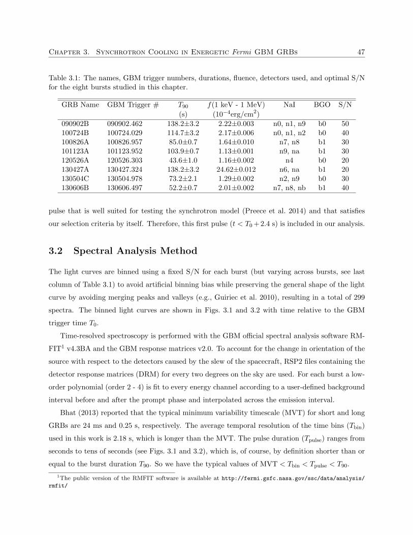
Chapter 3. Synchrotron Cooling in Energetic Fermi GBM GRBs 47
Table 3.1: The names, GBM trigger numbers, durations, fluence, detectors used, and optimal S/Nfor the eight bursts studied in this chapter.
GRB Name GBM Trigger # T90 f(1 keV - 1 MeV) NaI BGO S/N
(s) (10−4erg/cm2)
090902B 090902.462 138.2±3.2 2.22±0.003 n0, n1, n9 b0 50100724B 100724.029 114.7±3.2 2.17±0.006 n0, n1, n2 b0 40100826A 100826.957 85.0±0.7 1.64±0.010 n7, n8 b1 30101123A 101123.952 103.9±0.7 1.13±0.001 n9, na b1 30120526A 120526.303 43.6±1.0 1.16±0.002 n4 b0 20130427A 130427.324 138.2±3.2 24.62±0.012 n6, na b1 20130504C 130504.978 73.2±2.1 1.29±0.002 n2, n9 b0 30130606B 130606.497 52.2±0.7 2.01±0.002 n7, n8, nb b1 40
pulse that is well suited for testing the synchrotron model (Preece et al. 2014) and that satisfies
our selection criteria by itself. Therefore, this first pulse (t < T0 + 2.4 s) is included in our analysis.
3.2 Spectral Analysis Method
The light curves are binned using a fixed S/N for each burst (but varying across bursts, see last
column of Table 3.1) to avoid artificial binning bias while preserving the general shape of the light
curve by avoiding merging peaks and valleys (e.g., Guiriec et al. 2010), resulting in a total of 299
spectra. The binned light curves are shown in Figs. 3.1 and 3.2 with time relative to the GBM
trigger time T0.
Time-resolved spectroscopy is performed with the GBM official spectral analysis software RM-
FIT1 v4.3BA and the GBM response matrices v2.0. To account for the change in orientation of the
source with respect to the detectors caused by the slew of the spacecraft, RSP2 files containing the
detector response matrices (DRM) for every two degrees on the sky are used. For each burst a low-
order polynomial (order 2 - 4) is fit to every energy channel according to a user-defined background
interval before and after the prompt phase and interpolated across the emission interval.
Bhat (2013) reported that the typical minimum variability timescale (MVT) for short and long
GRBs are 24 ms and 0.25 s, respectively. The average temporal resolution of the time bins (Tbin)
used in this work is 2.18 s, which is longer than the MVT. The pulse duration (Tpulse) ranges from
seconds to tens of seconds (see Figs. 3.1 and 3.2), which is, of course, by definition shorter than or
equal to the burst duration T90. So we have the typical values of MVT < Tbin < Tpulse < T90.
1The public version of the RMFIT software is available at http://fermi.gsfc.nasa.gov/ssc/data/analysis/
rmfit/
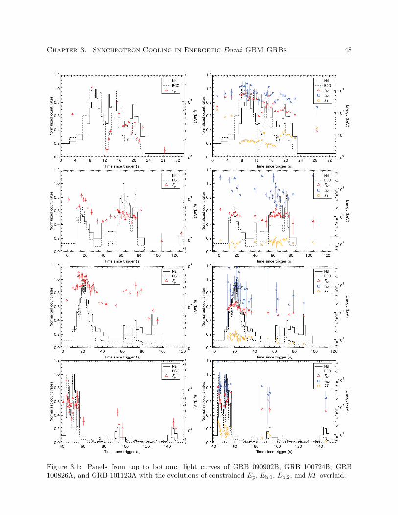
Chapter 3. Synchrotron Cooling in Energetic Fermi GBM GRBs 48
Figure 3.1: Panels from top to bottom: light curves of GRB 090902B, GRB 100724B, GRB100826A, and GRB 101123A with the evolutions of constrained Ep, Eb,1, Eb,2, and kT overlaid.
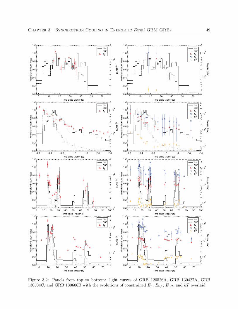
Chapter 3. Synchrotron Cooling in Energetic Fermi GBM GRBs 49
Figure 3.2: Panels from top to bottom: light curves of GRB 120526A, GRB 130427A, GRB130504C, and GRB 130606B with the evolutions of constrained Ep, Eb,1, Eb,2, and kT overlaid.
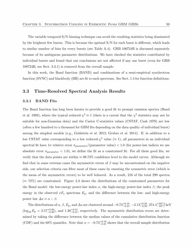
Chapter 3. Synchrotron Cooling in Energetic Fermi GBM GRBs 50
The variable temporal S/N binning technique can avoid the resulting statistics being dominated
by the brightest few bursts. This is because the optimal S/N for each burst is different, which leads
to similar number of bins for every bursts (see Table A.4). GRB 100724B is discussed separately
because of its ambiguous parameter distributions. We have checked the statistics contributed by
individual bursts and found that our conclusions are not affected if any one burst (even for GRB
100724B, see Sect. 3.3.1) is removed from the overall sample.
In this work, the Band function (BAND) and combinations of a semi-empirical synchrotron
function (SYNC) and blackbody (BB) are fit to each spectrum. See Sect. 1.4 for function definitions.
3.3 Time-Resolved Spectral Analysis Results
3.3.1 BAND Fits
The Band function has long been known to provide a good fit to prompt emission spectra (Band
et al. 1993), where the typical reduced-χ2 ≈ 1 (there is a caveat that the χ2 statistics may not be
suitable for non-Gaussian data) and the Castor C-statistics values (CSTAT, Cash 1979) are low
(often a few hundred to a thousand for GBM fits depending on the data quality of individual burst)
among the simplest models (e.g., Goldstein et al. 2012; Gruber et al. 2014). If, in addition to a
low CSTAT value corresponding to a low reduced-χ2 value (≈ 1), all parameters in an individual
spectral fit have 1σ relative error σparameter/(parameter value) < 1.0 (for power-law indices we use
absolute error σparameter < 1.0), we define the fit as a constrained fit. For all these good fits, we
verify that the data points are within ≈ 99.73% confidence level to the model curves. Although we
find that in some extreme cases the asymmetric errors of β may be unconstrained on the negative
side, our selection criteria can filter most of these cases by ensuring the symmetric error (which is
the mean of the asymmetric errors) to be well behaved. As a result, 216 of the total 299 spectra
(≈ 72%) are constrained. Figure 3.3 shows the distributions of the constrained parameters for
the Band model: the low-energy power-law index α, the high-energy power-law index β, the peak
energy in the observed νFν spectrum Ep, and the difference between the low- and high-energy
power law ∆s ≡ α− β.
The distributions of α, β, Ep, and ∆s are clustered around−0.73+0.16−0.21, −2.13+0.28
−0.56, 374.4+307.3−187.7 keV
(log10Ep = 2.57+0.26−0.30), and 1.38+0.54
−0.31, respectively. The asymmetric distribution errors are deter-
mined by taking the difference between the median values of the cumulative distribution function
(CDF) and the 68% quantiles. Note that α = −0.73+0.16−0.21 shows that the overall sample distribution
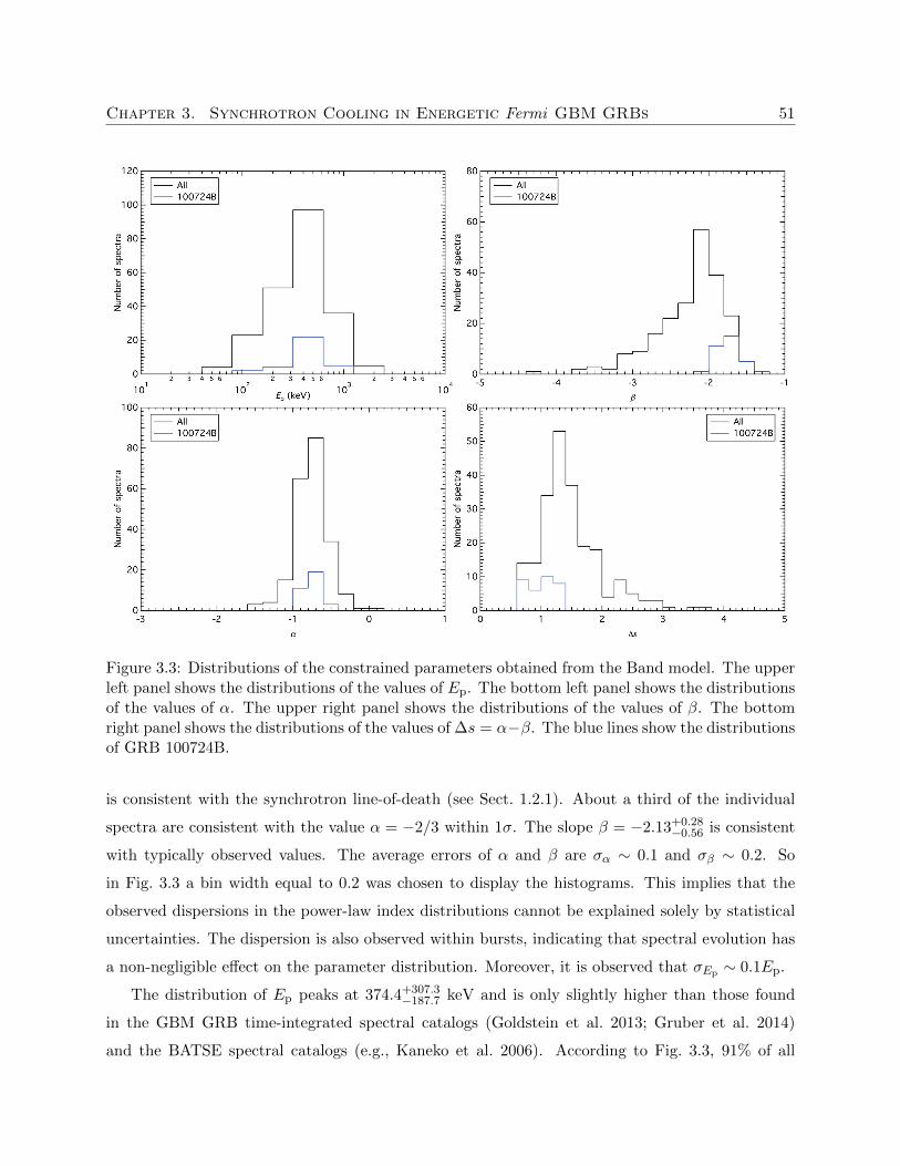
Chapter 3. Synchrotron Cooling in Energetic Fermi GBM GRBs 51
Figure 3.3: Distributions of the constrained parameters obtained from the Band model. The upperleft panel shows the distributions of the values of Ep. The bottom left panel shows the distributionsof the values of α. The upper right panel shows the distributions of the values of β. The bottomright panel shows the distributions of the values of ∆s = α−β. The blue lines show the distributionsof GRB 100724B.
is consistent with the synchrotron line-of-death (see Sect. 1.2.1). About a third of the individual
spectra are consistent with the value α = −2/3 within 1σ. The slope β = −2.13+0.28−0.56 is consistent
with typically observed values. The average errors of α and β are σα ∼ 0.1 and σβ ∼ 0.2. So
in Fig. 3.3 a bin width equal to 0.2 was chosen to display the histograms. This implies that the
observed dispersions in the power-law index distributions cannot be explained solely by statistical
uncertainties. The dispersion is also observed within bursts, indicating that spectral evolution has
a non-negligible effect on the parameter distribution. Moreover, it is observed that σEp ∼ 0.1Ep.
The distribution of Ep peaks at 374.4+307.3−187.7 keV and is only slightly higher than those found
in the GBM GRB time-integrated spectral catalogs (Goldstein et al. 2013; Gruber et al. 2014)
and the BATSE spectral catalogs (e.g., Kaneko et al. 2006). According to Fig. 3.3, 91% of all
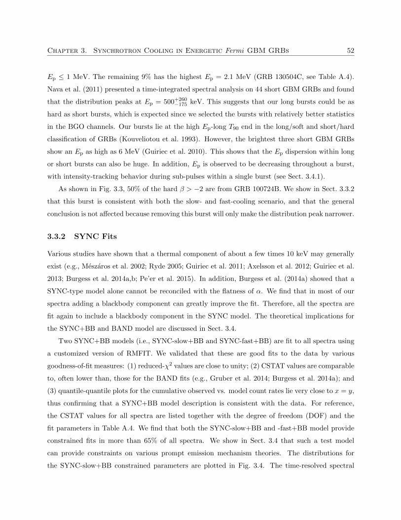
Chapter 3. Synchrotron Cooling in Energetic Fermi GBM GRBs 52
Ep ≤ 1 MeV. The remaining 9% has the highest Ep = 2.1 MeV (GRB 130504C, see Table A.4).
Nava et al. (2011) presented a time-integrated spectral analysis on 44 short GBM GRBs and found
that the distribution peaks at Ep = 500+260−175 keV. This suggests that our long bursts could be as
hard as short bursts, which is expected since we selected the bursts with relatively better statistics
in the BGO channels. Our bursts lie at the high Ep-long T90 end in the long/soft and short/hard
classification of GRBs (Kouveliotou et al. 1993). However, the brightest three short GBM GRBs
show an Ep as high as 6 MeV (Guiriec et al. 2010). This shows that the Ep dispersion within long
or short bursts can also be huge. In addition, Ep is observed to be decreasing throughout a burst,
with intensity-tracking behavior during sub-pulses within a single burst (see Sect. 3.4.1).
As shown in Fig. 3.3, 50% of the hard β > −2 are from GRB 100724B. We show in Sect. 3.3.2
that this burst is consistent with both the slow- and fast-cooling scenario, and that the general
conclusion is not affected because removing this burst will only make the distribution peak narrower.
3.3.2 SYNC Fits
Various studies have shown that a thermal component of about a few times 10 keV may generally
exist (e.g., Meszaros et al. 2002; Ryde 2005; Guiriec et al. 2011; Axelsson et al. 2012; Guiriec et al.
2013; Burgess et al. 2014a,b; Pe’er et al. 2015). In addition, Burgess et al. (2014a) showed that a
SYNC-type model alone cannot be reconciled with the flatness of α. We find that in most of our
spectra adding a blackbody component can greatly improve the fit. Therefore, all the spectra are
fit again to include a blackbody component in the SYNC model. The theoretical implications for
the SYNC+BB and BAND model are discussed in Sect. 3.4.
Two SYNC+BB models (i.e., SYNC-slow+BB and SYNC-fast+BB) are fit to all spectra using
a customized version of RMFIT. We validated that these are good fits to the data by various
goodness-of-fit measures: (1) reduced-χ2 values are close to unity; (2) CSTAT values are comparable
to, often lower than, those for the BAND fits (e.g., Gruber et al. 2014; Burgess et al. 2014a); and
(3) quantile-quantile plots for the cumulative observed vs. model count rates lie very close to x = y,
thus confirming that a SYNC+BB model description is consistent with the data. For reference,
the CSTAT values for all spectra are listed together with the degree of freedom (DOF) and the
fit parameters in Table A.4. We find that both the SYNC-slow+BB and -fast+BB model provide
constrained fits in more than 65% of all spectra. We show in Sect. 3.4 that such a test model
can provide constraints on various prompt emission mechanism theories. The distributions for
the SYNC-slow+BB constrained parameters are plotted in Fig. 3.4. The time-resolved spectral
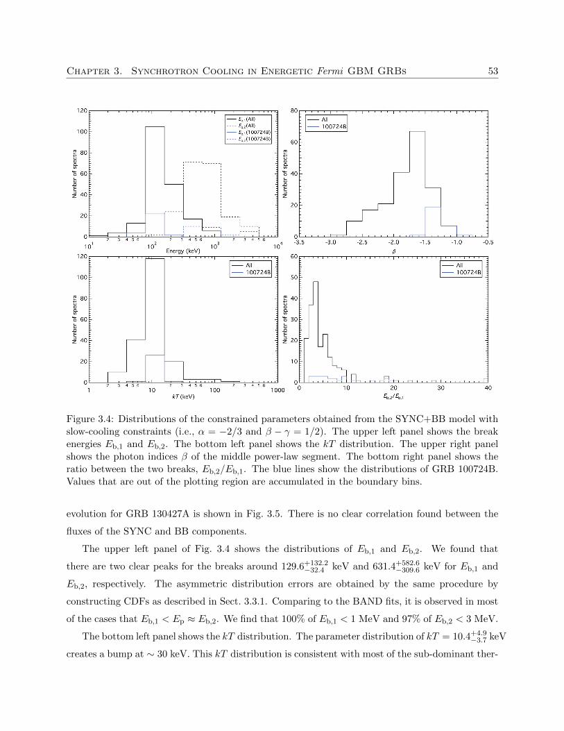
Chapter 3. Synchrotron Cooling in Energetic Fermi GBM GRBs 53
Figure 3.4: Distributions of the constrained parameters obtained from the SYNC+BB model withslow-cooling constraints (i.e., α = −2/3 and β − γ = 1/2). The upper left panel shows the breakenergies Eb,1 and Eb,2. The bottom left panel shows the kT distribution. The upper right panelshows the photon indices β of the middle power-law segment. The bottom right panel shows theratio between the two breaks, Eb,2/Eb,1. The blue lines show the distributions of GRB 100724B.Values that are out of the plotting region are accumulated in the boundary bins.
evolution for GRB 130427A is shown in Fig. 3.5. There is no clear correlation found between the
fluxes of the SYNC and BB components.
The upper left panel of Fig. 3.4 shows the distributions of Eb,1 and Eb,2. We found that
there are two clear peaks for the breaks around 129.6+132.2−32.4 keV and 631.4+582.6
−309.6 keV for Eb,1 and
Eb,2, respectively. The asymmetric distribution errors are obtained by the same procedure by
constructing CDFs as described in Sect. 3.3.1. Comparing to the BAND fits, it is observed in most
of the cases that Eb,1 < Ep ≈ Eb,2. We find that 100% of Eb,1 < 1 MeV and 97% of Eb,2 < 3 MeV.
The bottom left panel shows the kT distribution. The parameter distribution of kT = 10.4+4.9−3.7 keV
creates a bump at ∼ 30 keV. This kT distribution is consistent with most of the sub-dominant ther-
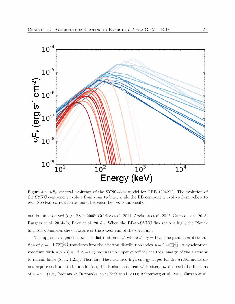
Chapter 3. Synchrotron Cooling in Energetic Fermi GBM GRBs 54
Figure 3.5: νFν spectral evolution of the SYNC-slow model for GRB 130427A. The evolution ofthe SYNC component evolves from cyan to blue, while the BB component evolves from yellow tored. No clear correlation is found between the two components.
mal bursts observed (e.g., Ryde 2005; Guiriec et al. 2011; Axelsson et al. 2012; Guiriec et al. 2013;
Burgess et al. 2014a,b; Pe’er et al. 2015). When the BB-to-SYNC flux ratio is high, the Planck
function dominates the curvature of the lowest end of the spectrum.
The upper right panel shows the distribution of β, where β− γ = 1/2. The parameter distribu-
tion of β = −1.72+0.48−0.25 translates into the electron distribution index p = 2.44+0.50
−0.96. A synchrotron
spectrum with p > 2 (i.e., β < −1.5) requires no upper cutoff for the total energy of the electrons
to remain finite (Sect. 1.2.1). Therefore, the measured high-energy slopes for the SYNC model do
not require such a cutoff. In addition, this is also consistent with afterglow-deduced distributions
of p ∼ 2.3 (e.g., Bednarz & Ostrowski 1998; Kirk et al. 2000; Achterberg et al. 2001; Curran et al.
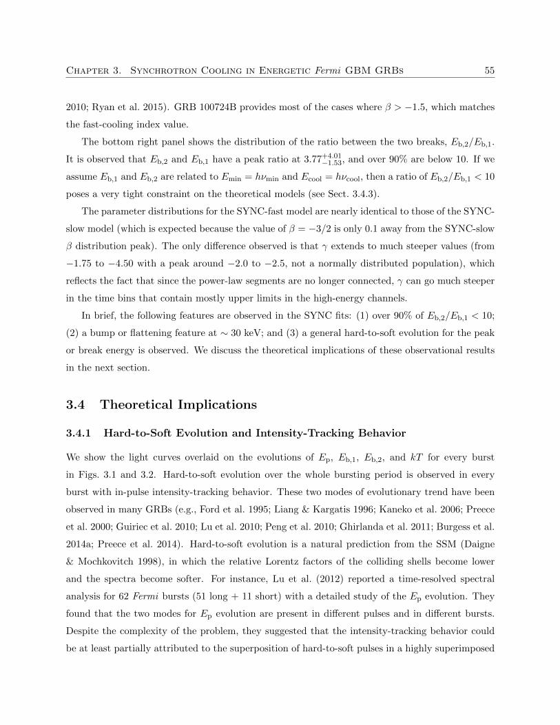
Chapter 3. Synchrotron Cooling in Energetic Fermi GBM GRBs 55
2010; Ryan et al. 2015). GRB 100724B provides most of the cases where β > −1.5, which matches
the fast-cooling index value.
The bottom right panel shows the distribution of the ratio between the two breaks, Eb,2/Eb,1.
It is observed that Eb,2 and Eb,1 have a peak ratio at 3.77+4.01−1.53, and over 90% are below 10. If we
assume Eb,1 and Eb,2 are related to Emin = hνmin and Ecool = hνcool, then a ratio of Eb,2/Eb,1 < 10
poses a very tight constraint on the theoretical models (see Sect. 3.4.3).
The parameter distributions for the SYNC-fast model are nearly identical to those of the SYNC-
slow model (which is expected because the value of β = −3/2 is only 0.1 away from the SYNC-slow
β distribution peak). The only difference observed is that γ extends to much steeper values (from
−1.75 to −4.50 with a peak around −2.0 to −2.5, not a normally distributed population), which
reflects the fact that since the power-law segments are no longer connected, γ can go much steeper
in the time bins that contain mostly upper limits in the high-energy channels.
In brief, the following features are observed in the SYNC fits: (1) over 90% of Eb,2/Eb,1 < 10;
(2) a bump or flattening feature at ∼ 30 keV; and (3) a general hard-to-soft evolution for the peak
or break energy is observed. We discuss the theoretical implications of these observational results
in the next section.
3.4 Theoretical Implications
3.4.1 Hard-to-Soft Evolution and Intensity-Tracking Behavior
We show the light curves overlaid on the evolutions of Ep, Eb,1, Eb,2, and kT for every burst
in Figs. 3.1 and 3.2. Hard-to-soft evolution over the whole bursting period is observed in every
burst with in-pulse intensity-tracking behavior. These two modes of evolutionary trend have been
observed in many GRBs (e.g., Ford et al. 1995; Liang & Kargatis 1996; Kaneko et al. 2006; Preece
et al. 2000; Guiriec et al. 2010; Lu et al. 2010; Peng et al. 2010; Ghirlanda et al. 2011; Burgess et al.
2014a; Preece et al. 2014). Hard-to-soft evolution is a natural prediction from the SSM (Daigne
& Mochkovitch 1998), in which the relative Lorentz factors of the colliding shells become lower
and the spectra become softer. For instance, Lu et al. (2012) reported a time-resolved spectral
analysis for 62 Fermi bursts (51 long + 11 short) with a detailed study of the Ep evolution. They
found that the two modes for Ep evolution are present in different pulses and in different bursts.
Despite the complexity of the problem, they suggested that the intensity-tracking behavior could
be at least partially attributed to the superposition of hard-to-soft pulses in a highly superimposed
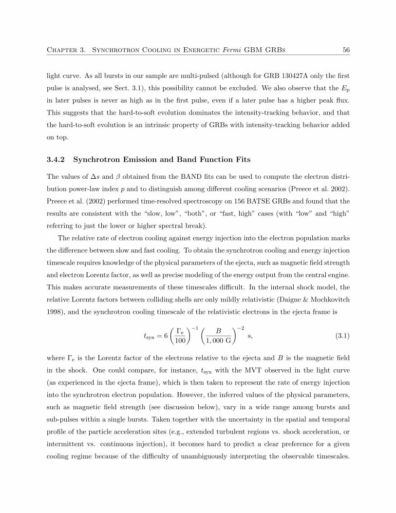
Chapter 3. Synchrotron Cooling in Energetic Fermi GBM GRBs 56
light curve. As all bursts in our sample are multi-pulsed (although for GRB 130427A only the first
pulse is analysed, see Sect. 3.1), this possibility cannot be excluded. We also observe that the Ep
in later pulses is never as high as in the first pulse, even if a later pulse has a higher peak flux.
This suggests that the hard-to-soft evolution dominates the intensity-tracking behavior, and that
the hard-to-soft evolution is an intrinsic property of GRBs with intensity-tracking behavior added
on top.
3.4.2 Synchrotron Emission and Band Function Fits
The values of ∆s and β obtained from the BAND fits can be used to compute the electron distri-
bution power-law index p and to distinguish among different cooling scenarios (Preece et al. 2002).
Preece et al. (2002) performed time-resolved spectroscopy on 156 BATSE GRBs and found that the
results are consistent with the “slow, low”, “both”, or “fast, high” cases (with “low” and “high”
referring to just the lower or higher spectral break).
The relative rate of electron cooling against energy injection into the electron population marks
the difference between slow and fast cooling. To obtain the synchrotron cooling and energy injection
timescale requires knowledge of the physical parameters of the ejecta, such as magnetic field strength
and electron Lorentz factor, as well as precise modeling of the energy output from the central engine.
This makes accurate measurements of these timescales difficult. In the internal shock model, the
relative Lorentz factors between colliding shells are only mildly relativistic (Daigne & Mochkovitch
1998), and the synchrotron cooling timescale of the relativistic electrons in the ejecta frame is
tsyn = 6
(Γe
100
)−1( B
1, 000 G
)−2
s, (3.1)
where Γe is the Lorentz factor of the electrons relative to the ejecta and B is the magnetic field
in the shock. One could compare, for instance, tsyn with the MVT observed in the light curve
(as experienced in the ejecta frame), which is then taken to represent the rate of energy injection
into the synchrotron electron population. However, the inferred values of the physical parameters,
such as magnetic field strength (see discussion below), vary in a wide range among bursts and
sub-pulses within a single bursts. Taken together with the uncertainty in the spatial and temporal
profile of the particle acceleration sites (e.g., extended turbulent regions vs. shock acceleration, or
intermittent vs. continuous injection), it becomes hard to predict a clear preference for a given
cooling regime because of the difficulty of unambiguously interpreting the observable timescales.
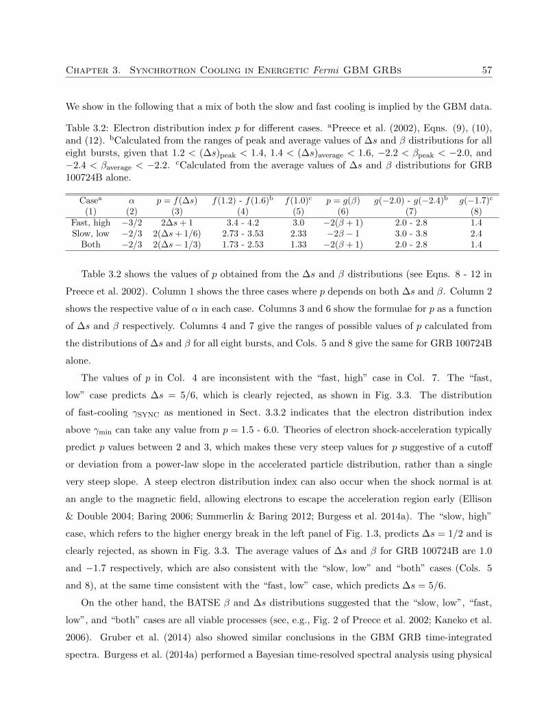
Chapter 3. Synchrotron Cooling in Energetic Fermi GBM GRBs 57
We show in the following that a mix of both the slow and fast cooling is implied by the GBM data.
Table 3.2: Electron distribution index p for different cases. aPreece et al. (2002), Eqns. (9), (10),and (12). bCalculated from the ranges of peak and average values of ∆s and β distributions for alleight bursts, given that 1.2 < (∆s)peak < 1.4, 1.4 < (∆s)average < 1.6, −2.2 < βpeak < −2.0, and−2.4 < βaverage < −2.2. cCalculated from the average values of ∆s and β distributions for GRB100724B alone.
Casea α p = f(∆s) f(1.2) - f(1.6)b f(1.0)c p = g(β) g(−2.0) - g(−2.4)b g(−1.7)c
(1) (2) (3) (4) (5) (6) (7) (8)Fast, high −3/2 2∆s+ 1 3.4 - 4.2 3.0 −2(β + 1) 2.0 - 2.8 1.4Slow, low −2/3 2(∆s+ 1/6) 2.73 - 3.53 2.33 −2β − 1 3.0 - 3.8 2.4
Both −2/3 2(∆s− 1/3) 1.73 - 2.53 1.33 −2(β + 1) 2.0 - 2.8 1.4
Table 3.2 shows the values of p obtained from the ∆s and β distributions (see Eqns. 8 - 12 in
Preece et al. 2002). Column 1 shows the three cases where p depends on both ∆s and β. Column 2
shows the respective value of α in each case. Columns 3 and 6 show the formulae for p as a function
of ∆s and β respectively. Columns 4 and 7 give the ranges of possible values of p calculated from
the distributions of ∆s and β for all eight bursts, and Cols. 5 and 8 give the same for GRB 100724B
alone.
The values of p in Col. 4 are inconsistent with the “fast, high” case in Col. 7. The “fast,
low” case predicts ∆s = 5/6, which is clearly rejected, as shown in Fig. 3.3. The distribution
of fast-cooling γSYNC as mentioned in Sect. 3.3.2 indicates that the electron distribution index
above γmin can take any value from p = 1.5 - 6.0. Theories of electron shock-acceleration typically
predict p values between 2 and 3, which makes these very steep values for p suggestive of a cutoff
or deviation from a power-law slope in the accelerated particle distribution, rather than a single
very steep slope. A steep electron distribution index can also occur when the shock normal is at
an angle to the magnetic field, allowing electrons to escape the acceleration region early (Ellison
& Double 2004; Baring 2006; Summerlin & Baring 2012; Burgess et al. 2014a). The “slow, high”
case, which refers to the higher energy break in the left panel of Fig. 1.3, predicts ∆s = 1/2 and is
clearly rejected, as shown in Fig. 3.3. The average values of ∆s and β for GRB 100724B are 1.0
and −1.7 respectively, which are also consistent with the “slow, low” and “both” cases (Cols. 5
and 8), at the same time consistent with the “fast, low” case, which predicts ∆s = 5/6.
On the other hand, the BATSE β and ∆s distributions suggested that the “slow, low”, “fast,
low”, and “both” cases are all viable processes (see, e.g., Fig. 2 of Preece et al. 2002; Kaneko et al.
2006). Gruber et al. (2014) also showed similar conclusions in the GBM GRB time-integrated
spectra. Burgess et al. (2014a) performed a Bayesian time-resolved spectral analysis using physical
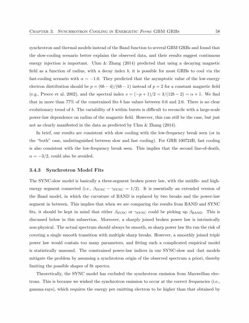
Chapter 3. Synchrotron Cooling in Energetic Fermi GBM GRBs 58
synchrotron and thermal models instead of the Band function to several GBM GRBs and found that
the slow-cooling scenario better explains the observed data, and their results suggest continuous
energy injection is important. Uhm & Zhang (2014) predicted that using a decaying magnetic
field as a function of radius, with a decay index b, it is possible for most GRBs to cool via the
fast-cooling scenario with α ∼ −1.0. They predicted that the asymptotic value of the low-energy
electron distribution should be p = (6b− 4)/(6b− 1) instead of p = 2 for a constant magnetic field
(e.g., Preece et al. 2002), and the spectral index s = (−p + 1)/2 = 3/(12b − 2) = α + 1. We find
that in more than 77% of the constrained fits b has values between 0.6 and 2.6. There is no clear
evolutionary trend of b. The variability of b within bursts is difficult to reconcile with a large-scale
power-law dependence on radius of the magnetic field. However, this can still be the case, but just
not as clearly manifested in the data as predicted by Uhm & Zhang (2014).
In brief, our results are consistent with slow cooling with the low-frequency break seen (or in
the “both” case, undistinguished between slow and fast cooling). For GRB 100724B, fast cooling
is also consistent with the low-frequency break seen. This implies that the second line-of-death,
α = −3/2, could also be avoided.
3.4.3 Synchrotron Model Fits
The SYNC-slow model is basically a three-segment broken power law, with the middle- and high-
energy segment connected (i.e., βSYNC − γSYNC = 1/2). It is essentially an extended version of
the Band model, in which the curvature of BAND is replaced by two breaks and the power-law
segment in between. This implies that when we are comparing the results from BAND and SYNC
fits, it should be kept in mind that either βSYNC or γSYNC could be picking up βBAND. This is
discussed below in this subsection. Moreover, a sharply joined broken power law is intrinsically
non-physical. The actual spectrum should always be smooth, so sharp power law fits run the risk of
covering a single smooth transition with multiple sharp breaks. However, a smoothly joined triple
power law would contain too many parameters, and fitting such a complicated empirical model
is statistically unsound. The constrained power-law indices in our SYNC-slow and -fast models
mitigate the problem by assuming a synchrotron origin of the observed spectrum a priori, thereby
limiting the possible shapes of fit spectra.
Theoretically, the SYNC model has excluded the synchrotron emission from Maxwellian elec-
trons. This is because we wished the synchrotron emission to occur at the correct frequencies (i.e.,
gamma-rays), which requires the energy per emitting electron to be higher than that obtained by
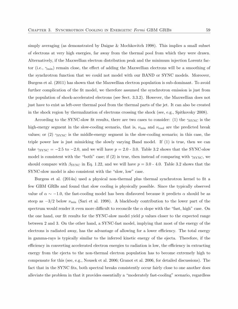
Chapter 3. Synchrotron Cooling in Energetic Fermi GBM GRBs 59
simply averaging (as demonstrated by Daigne & Mochkovitch 1998). This implies a small subset
of electrons at very high energies, far away from the thermal pool from which they were drawn.
Alternatively, if the Maxwellian electron distribution peak and the minimum injection Lorentz fac-
tor (i.e., γmin) remain close, the effect of adding the Maxwellian electrons will be a smoothing of
the synchrotron function that we could not model with our BAND or SYNC models. Moreover,
Burgess et al. (2011) has shown that the Maxwellian electron population is sub-dominant. To avoid
further complication of the fit model, we therefore assumed the synchrotron emission is just from
the population of shock-accelerated electrons (see Sect. 3.3.2). However, the Maxwellian does not
just have to exist as left-over thermal pool from the thermal parts of the jet. It can also be created
in the shock region by thermalization of electrons crossing the shock (see, e.g., Spitkovsky 2008).
According to the SYNC-slow fit results, there are two cases to consider: (1) the γSYNC is the
high-energy segment in the slow-cooling scenario, that is, νmin and νcool are the predicted break
values; or (2) γSYNC is the middle-energy segment in the slow-cooling scenario; in this case, the
triple power law is just mimicking the slowly varying Band model. If (1) is true, then we can
take γSYNC = −2.5 to −2.0, and we will have p = 2.0 - 3.0. Table 3.2 shows that the SYNC-slow
model is consistent with the “both” case; if (2) is true, then instead of comparing with γSYNC, we
should compare with βSYNC in Eq. 1.22, and we will have p = 3.0 - 4.0. Table 3.2 shows that the
SYNC-slow model is also consistent with the “slow, low” case.
Burgess et al. (2014a) used a physical non-thermal plus thermal synchrotron kernel to fit a
few GBM GRBs and found that slow cooling is physically possible. Since the typically observed
value of α ∼ −1.0, the fast-cooling model has been disfavored because it predicts α should be as
steep as −3/2 below νmin (Sari et al. 1998). A blackbody contribution to the lower part of the
spectrum would render it even more difficult to reconcile the α slope with the “fast, high” case. On
the one hand, our fit results for the SYNC-slow model yield p values closer to the expected range
between 2 and 3. On the other hand, a SYNC-fast model, implying that most of the energy of the
electrons is radiated away, has the advantage of allowing for a lower efficiency. The total energy
in gamma-rays is typically similar to the inferred kinetic energy of the ejecta. Therefore, if the
efficiency in converting accelerated electron energies to radiation is low, the efficiency in extracting
energy from the ejecta to the non-thermal electron population has to become extremely high to
compensate for this (see, e.g., Nousek et al. 2006; Granot et al. 2006, for detailed discussions). The
fact that in the SYNC fits, both spectral breaks consistently occur fairly close to one another does
alleviate the problem in that it provides essentially a “moderately fast-cooling” scenario, regardless
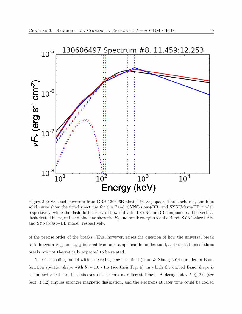
Chapter 3. Synchrotron Cooling in Energetic Fermi GBM GRBs 60
Figure 3.6: Selected spectrum from GRB 130606B plotted in νFν space. The black, red, and bluesolid curve show the fitted spectrum for the Band, SYNC-slow+BB, and SYNC-fast+BB model,respectively, while the dash-dotted curves show individual SYNC or BB components. The verticaldash-dotted black, red, and blue line show the Ep and break energies for the Band, SYNC-slow+BB,and SYNC-fast+BB model, respectively.
of the precise order of the breaks. This, however, raises the question of how the universal break
ratio between νmin and νcool inferred from our sample can be understood, as the positions of these
breaks are not theoretically expected to be related.
The fast-cooling model with a decaying magnetic field (Uhm & Zhang 2014) predicts a Band
function spectral shape with b ∼ 1.0 - 1.5 (see their Fig. 4), in which the curved Band shape is
a summed effect for the emissions of electrons at different times. A decay index b . 2.6 (see
Sect. 3.4.2) implies stronger magnetic dissipation, and the electrons at later time could be cooled
Chapter 3. Synchrotron Cooling in Energetic Fermi GBM GRBs 61
by slow cooling, thus the positions of νcool and νmin could reverse and move closer to each other, so
that the “both” case is possible. Uhm & Zhang (2014) showed that this is possible on a timescale
∼ 1.0 s, consistent with the typical Tbin used in this work (see Sect. 3.1). We find that the BAND
and SYNC model have very similar shapes (Fig. 3.6) that are consistent with this interpretation
and thus provide further support for the “both” case.
3.4.4 Thermal Origin of Prompt Emission
Recently, Beloborodov (2013) suggested that the evolution of Ep could be a manifestation of thermal
emission. As shown in Fig. 3.3, more than 90% of Ep values remain below 1 MeV. The observed
clustering of Ep ∼ few hundred keV, instead of a wide distribution, is hard to explain in the
SSM. The observed spectral width in the νFν space is log(E1/E2) ≈ 1.0 - 1.5 decades in photon
energy (Beloborodov 2013), where E2 − E1 is the width at half-maximum. This is narrower than
a synchrotron model would predict (Daigne et al. 2011).
Early photospheric models assumed a freely expanding radiation-dominated outflow with no
baryonic loading or magnetic field (Goodman 1986; Paczynski 1986). This predicts a sharply
defined peak with a Planck spectrum (Beloborodov 2011), which contradicts the observed non-
thermal spectra in most GRBs. Detailed radiation transfer simulations have shown that a thermal
origin of the Band function is possible (Pe’er et al. 2006; Giannios 2008; Beloborodov 2010; Vurm
et al. 2011), and Beloborodov (2013) computed that the maximum Ep of a spectrum from thermal
plasma is given by 30ΓP keV under high radiation efficiency, where ΓP is the Lorentz factor of the
Planckian photospheric shell. With the typical values of the Lorentz factor of GRBs to be ∼ 100,
Ep,max ∼ 3 MeV in the rest frame. This value is consistent with most of our observed Ep . 500 keV,
but only when assuming a redshift z . 0.83. Deng & Zhang (2014) also found that α ∼ −1.0 could
be achieved if the radiating photosphere has a constant or increasing luminosity. However, they
stated that it is difficult to reproduce the observed hard-to-soft evolution under natural conditions.
3.5 Conclusions
We performed time-resolved spectroscopy for eight energetic, long GRBs observed by Fermi GBM
during the first five years of its mission. We obtained well-constrained Band spectral parameters
and studied their theoretical implications. We showed that even in the bursts with good high-energy
statistics above 900 keV, most observed properties can be explained using the synchrotron shock
Chapter 3. Synchrotron Cooling in Energetic Fermi GBM GRBs 62
model. We also tested the observed spectra with a synchrotron plus blackbody model using slow-
and fast-cooling parametric constraints, and found that the “both” case is consistent with the data,
which requires a narrow distribution of the break ratio Eb,2/Eb,1 < 10 with a peak at 3.77+4.01−1.53.
The population of p is found to be 2 - 3, in accordance with the expected range. The picture of a
“moderately fast-cooling” scenario can also explain the narrow distribution of the break ratio and
relax the efficiency problem for the slow-cooling scenario.
Recently, Frontera et al. (2013) reported the result of the time-resolved spectral analysis of
four GRBs observed by BATSE and BeppoSAX. They found that a specially devised empirical
Comptonized model is the best-fit model to most of their time-resolved spectra. They also found
that using a simple power law plus blackbody model (PL + BB) does not give fit results better than
the conventional Band function. This is consistent with the results from the Fermi GBM GRB
time-resolved spectral catalog (Yu et al. submitted) that most of the time-resolved spectra are best
fit by the Comptonized model, and only very few spectra are best fit by PL + BB, although they
are generally acceptable fits. We showed that the spectral shape & 1 MeV could be harder than a
Comptonized model or simple power law.
Our results confirmed that while most properties of energetic GRBs can be explained in the
conventional theoretical models, the radiative process in GRB prompt emission is complicated and
cannot be fully explained by a single distribution of electrons (e.g., due to anisotropic distribution of
electron energies or continuous acceleration or photospheric emission). The possibility of a decaying
magnetic field that modifies the fast-cooling spectrum was also explored, yielding a magnetic field
decay index 0.6 < b < 2.6 for 77% of the constrained fits. However, it is difficult to reconcile the
variability of b within bursts with a mechanism where the spectra are shaped by a single large-scale
decaying magnetic field. Nevertheless, such a field might still exist, but its impact may be obscured
by more local conditions in the flow.
Chapter 4
The Sharpness of GRB Prompt
Emission Spectra
“Study hard what interests you the most in the most
undisciplined, irreverent and original manner
possible.”
- Richard Feynman
The prompt emission of gamma-ray bursts (GRBs) is one of the most puzzling observed astro-
nomical phenomena. Since the discovery of GRBs in 1967 (Klebesadel et al. 1973), many emission
models have been proposed in order to explain the prompt phase of gamma-ray emission. This
phase consists of gamma-rays mainly within tens to a few hundred keV, in some cases as high as a
few thousand keV, lasting from a few milliseconds to hundreds of seconds.
Gamma-ray bursts are distributed isotropically (Briggs et al. 1996; Hakkila et al. 1994; Tegmark
et al. 1996) and cosmologically (Metzger et al. 1997; Waxman 1997a) over the sky. Despite the
last 45 years of research efforts, the dominant emission mechanism of these cosmological sources is
still controversial. Synchrotron radiation from a simple electron population is one of the simplest
physical phenomena that may be able to produce the observed spectral slopes of the Band function
(Band et al. 1993) that is commonly used to describe the photon spectra of GRB prompt emission.
The Band function is an empirical mathematical function consisting of two segments of power
laws, described by the low- and high-energy photon indices α and β, connected at the peak energy
parameterized as Ep. This peak energy has been observed typically at hundreds of keV (Kaneko
et al. 2006; Nava et al. 2011; Goldstein et al. 2012, 2013; Gruber et al. 2014). In what is known as
63
Chapter 4. The Sharpness of GRB Prompt Emission Spectra 64
the fireball model (Goodman 1986; Meszaros et al. 1993; Meszaros & Rees 1993; Rees & Meszaros
1992, 1994; Tavani 1996; Piran 1999), there are ejected shells with different bulk Lorentz factors.
When the faster shells catch up with the slower shells, internal shock waves will be produced.
The electrons in the shocked region of the shells are accelerated and their energy is radiated via
synchrotron emission in the local magnetic field.
The Band function’s two power-law indices are usually compared to the slopes of various radi-
ation models, leading to the discovery of the so-called line-of-death problem (Katz 1994a; Crider
et al. 1998; Preece et al. 1998a, 2002; Tavani 1995) for the synchrotron theory. When a power-
law distribution of electron energies is combined with synchrotron radiation theory, the low-energy
power-law photon index is −2/3. The fact that a fraction of observed α > −2/3 indicates that,
at least in some cases, the synchrotron explanation of GRB prompt spectra can be problematic,
because the observed spectra rise faster. The observed violations of the line-of-death are typically
around 30%. Recently, Burgess et al. (2015) used the Band function to fit a large number of sim-
ulated slow-cooling synchrotron spectra (with spectral peak determined by injection energy of the
electrons rather than their energy losses, as in the fast-cooling case), concluding that, in practice,
the line-of-death may be steeper, α > −0.8, than the value of α > −2/3. Moreover, they found that
the Band function cannot recover the simulated synchrotron peaks and power-law indices. These
findings all question the validity of using the synchrotron theories to explain the Band parameters.
Instead of fitting the empirical Band function to the spectra, Burgess et al. (2014a) used a syn-
chrotron function in the fitting process, combining the slow-cooling scenario with thermal emission.
Yu et al. (Ch. 3, 2015a) used a double broken power law to fit eight bright GRBs, in which they
found that the line-of-death problem could be alleviated in a moderately fast-cooling scenario, in
which the fast- and slow-cooling electrons are mixed together, usually with a blackbody compo-
nent at tens of keV or in a varying magnetic field. However, no single synchrotron model could
completely explain all the spectral properties of GRB prompt emission.
In this work we study the sharpness of the synchrotron emission spectrum in comparison to time-
resolved spectra of GRBs, a question recently raised by Beloborodov (2013); Vurm & Beloborodov
(2015). Our approach focuses on the curvature of the region capturing the peak or break energy
in the GRB prompt spectra by re-fitting all the spectra in an energy domain depending on this
peak or break, using the burst sample from the Fermi GBM GRB time-resolved spectral catalog
(Ch. 2, Yu et al. submitted). By comparing the spectral sharpness of the observed spectra to
various physical emission models, we are able to directly determine whether a model is capable of
Chapter 4. The Sharpness of GRB Prompt Emission Spectra 65
accounting for the peak emission of the observed spectra. By concentrating on the spectral peak
or break, we avoid potential issues with interpretation of the asymptotes of the fit functions, which
might lie outside the observable domain or be contaminated by additional radiative processes or
instrumental effects.
Thanks to the high-quality gamma-ray data obtained by Fermi GBM (Meegan et al. 2009),
which provides wide energy coverage and fine temporal and spectral resolutions, this is the first
time that we can directly compare the curvature of a large number of time-resolved spectra to
that of physical models, so that statistically significant conclusions about the prompt emission
mechanism can be drawn.
This chapter is structured as follows. In Section 4.1, we describe our analysis method. The
results are presented in Section 4.2. In Section 4.3, we check the consistency of our analysis. In
Section 4.4, we discuss the theoretical implications. The summary and conclusions are given in
Section 4.5.
We note that a recent independent study of the peak-flux GRB spectra (Axelsson & Borgonovo
2015) shows that a synchrotron function could be too wide for the observed Band shape. They
measured the full-width-half-maximum in the νFν spectra obtained from the 4-years Fermi GBM
GRB time-integrated spectral catalog (Gruber et al. 2014; von Kienlin et al. 2014) and the BATSE
5B GRB spectral catalog (Goldstein et al. 2013).
4.1 Spectral Sharpness Analysis Method
We take the BEST sample from Ch. 2 (Yu et al. submitted). Only the spectra best fit by the
Comptonized model (COMP), the Band function (BAND), and the smoothly broken power law
(SBPL) are included in the analysis. The functional forms of these models are given in Sect. 1.4.
This is because we are interested in comparing the sharpness around the peak or break energies
of theoretical models to the observed spectra. Thus, the 194 spectra best fit by a simple power
law or the power law plus blackbody, are excluded. All the 1,297 spectra best fit by either COMP,
BAND, or SBPL have convex shape (i.e., α > −2 for COMP and α > β for BAND and SBPL).
The best-fit model parameters for the 1,297 spectra are obtained from the catalog. Using the
catalog values of Ep, every spectrum is re-fit (using the same best fit function as in the catalog) in a
narrower energy domain that covers Ep (or the break energy Eb if there is no peak in the spectrum).
We refer this energy domain as the “data domain”, which contains the “triangle domain” (described
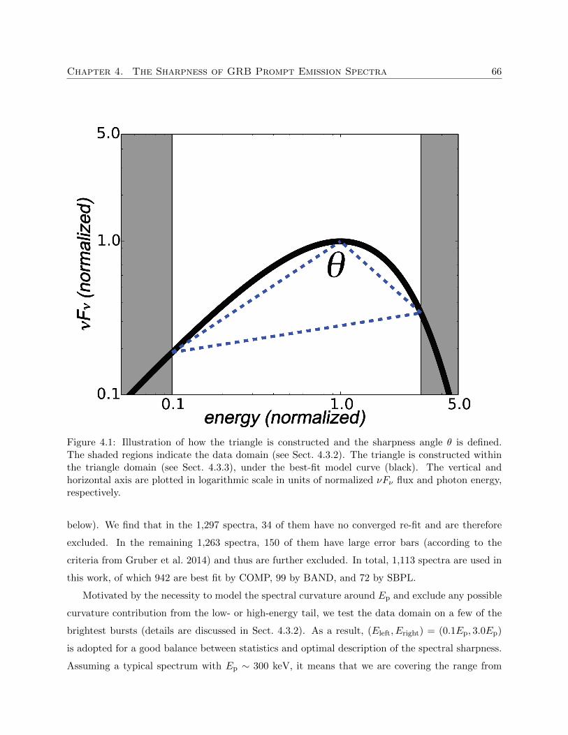
Chapter 4. The Sharpness of GRB Prompt Emission Spectra 66
Figure 4.1: Illustration of how the triangle is constructed and the sharpness angle θ is defined.The shaded regions indicate the data domain (see Sect. 4.3.2). The triangle is constructed withinthe triangle domain (see Sect. 4.3.3), under the best-fit model curve (black). The vertical andhorizontal axis are plotted in logarithmic scale in units of normalized νFν flux and photon energy,respectively.
below). We find that in the 1,297 spectra, 34 of them have no converged re-fit and are therefore
excluded. In the remaining 1,263 spectra, 150 of them have large error bars (according to the
criteria from Gruber et al. 2014) and thus are further excluded. In total, 1,113 spectra are used in
this work, of which 942 are best fit by COMP, 99 by BAND, and 72 by SBPL.
Motivated by the necessity to model the spectral curvature around Ep and exclude any possible
curvature contribution from the low- or high-energy tail, we test the data domain on a few of the
brightest bursts (details are discussed in Sect. 4.3.2). As a result, (Eleft, Eright) = (0.1Ep, 3.0Ep)
is adopted for a good balance between statistics and optimal description of the spectral sharpness.
Assuming a typical spectrum with Ep ∼ 300 keV, it means that we are covering the range from
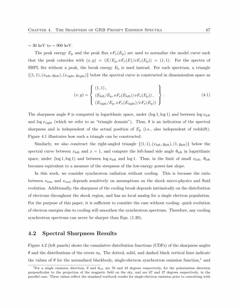
Chapter 4. The Sharpness of GRB Prompt Emission Spectra 67
∼ 30 keV to ∼ 900 keV.
The peak energy Ep and the peak flux νFν(Ep) are used to normalize the model curve such
that the peak coincides with (x, y) = (E/Ep, νFν(E)/νFν(Ep)) = (1, 1). For the spectra of
SBPL fits without a peak, the break energy Eb is used instead. For each spectrum, a triangle
(1, 1), (xleft, yleft), (xright, yright) below the spectral curve is constructed in dimensionless space as
(x, y) =
(1, 1) ,
(Eleft/Ep, νFν(Eleft)/νFν(Ep)) ,
(Eright/Ep, νFν(Eright)/νFν(Ep))
. (4.1)
The sharpness angle θ is computed in logarithmic space, under (log 1, log 1) and between log xleft
and log xright (which we refer to as “triangle domain”). Thus, θ is an indication of the spectral
sharpness and is independent of the actual position of Ep (i.e., also independent of redshift).
Figure 4.1 illustrates how such a triangle can be constructed.
Similarly, we also construct the right-angled triangle (1, 1), (xleft, yleft), (1, yleft) below the
spectral curve between xleft and x = 1, and compute the left-hand side angle θleft in logarithmic
space, under (log 1, log 1) and between log xleft and log 1. Thus, in the limit of small xleft, θleft
becomes equivalent to a measure of the steepness of the low-energy power-law slope.
In this work, we consider synchrotron radiation without cooling. This is because the ratio
between νmin and νcool depends sensitively on assumptions on the shock micro-physics and fluid
evolution. Additionally, the sharpness of the cooling break depends intrinsically on the distribution
of electrons throughout the shock region, and has no local analog for a single electron population.
For the purpose of this paper, it is sufficient to consider the case without cooling: quick evolution
of electron energies due to cooling will smoothen the synchrotron spectrum. Therefore, any cooling
synchrotron spectrum can never be sharper than Eqn. (1.20).
4.2 Spectral Sharpness Results
Figure 4.2 (left panels) shows the cumulative distribution functions (CDFs) of the sharpness angles
θ and the distributions of the errors σθ. The dotted, solid, and dashed black vertical lines indicate
the values of θ for the normalized blackbody, single-electron synchrotron emission function,1 and
1For a single emission direction, θ and θleft are 76 and 43 degrees respectively, for the polarization directionperpendicular to the projection of the magnetic field on the sky, and are 67 and 37 degrees respectively, in theparallel case. These values reflect the standard textbook results for single-electron emission prior to convolving with
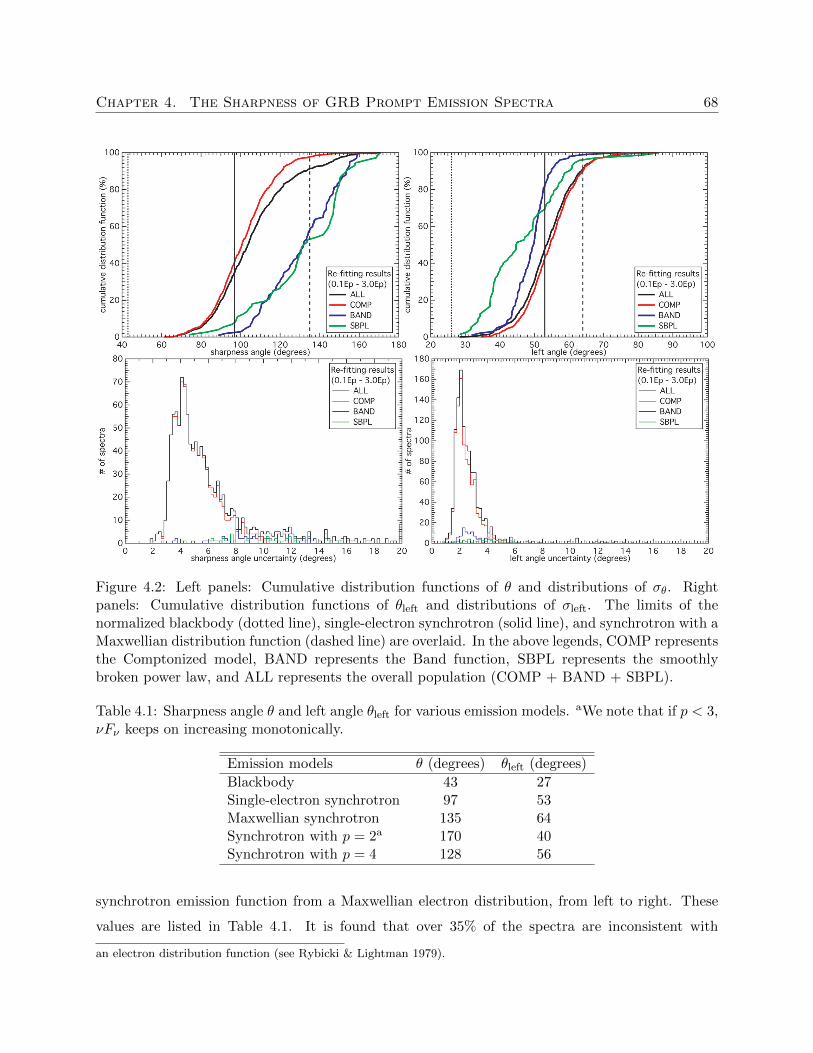
Chapter 4. The Sharpness of GRB Prompt Emission Spectra 68
Figure 4.2: Left panels: Cumulative distribution functions of θ and distributions of σθ. Rightpanels: Cumulative distribution functions of θleft and distributions of σleft. The limits of thenormalized blackbody (dotted line), single-electron synchrotron (solid line), and synchrotron with aMaxwellian distribution function (dashed line) are overlaid. In the above legends, COMP representsthe Comptonized model, BAND represents the Band function, SBPL represents the smoothlybroken power law, and ALL represents the overall population (COMP + BAND + SBPL).
Table 4.1: Sharpness angle θ and left angle θleft for various emission models. aWe note that if p < 3,νFν keeps on increasing monotonically.
Emission models θ (degrees) θleft (degrees)
Blackbody 43 27Single-electron synchrotron 97 53Maxwellian synchrotron 135 64Synchrotron with p = 2a 170 40Synchrotron with p = 4 128 56
synchrotron emission function from a Maxwellian electron distribution, from left to right. These
values are listed in Table 4.1. It is found that over 35% of the spectra are inconsistent with
an electron distribution function (see Rybicki & Lightman 1979).
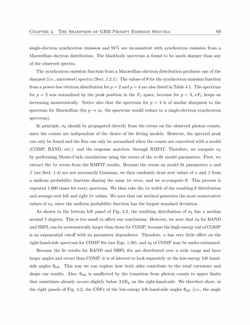
Chapter 4. The Sharpness of GRB Prompt Emission Spectra 69
single-electron synchrotron emission and 91% are inconsistent with synchrotron emission from a
Maxwellian electron distribution. The blackbody spectrum is found to be much sharper than any
of the observed spectra.
The synchrotron emission function from a Maxwellian electron distribution produces one of the
sharpest (i.e., narrowest) spectra (Sect. 1.2.1). The values of θ for the synchrotron emission function
from a power-law electron distribution for p = 2 and p = 4 are also listed in Table 4.1. The spectrum
for p = 2 was normalized by the peak position in the Fν space, because for p < 3, νFν keeps on
increasing monotonically. Notice also that the spectrum for p = 4 is of similar sharpness to the
spectrum for Maxwellian (for p→∞, the spectrum would reduce to a single-electron synchrotron
spectrum).
In principle, σθ should be propagated directly from the errors on the observed photon counts,
since the counts are independent of the choice of the fitting models. However, the spectral peak
can only be found and the flux can only be normalized when the counts are convolved with a model
(COMP, BAND, etc.) and the response matrices, through RMFIT. Therefore, we compute σθ
by performing Monte-Carlo simulations using the errors of the re-fit model parameters. First, we
extract the 1σ errors from the RMFIT results. Because the errors on model fit parameters α and
β (see Sect. 1.4) are not necessarily Gaussian, we then randomly draw new values of α and β from
a uniform probability function sharing the same 1σ error, and we re-compute θ. This process is
repeated 1,000 times for every spectrum. We then take the 1σ width of the resulting θ distribution
and average over left and right 1σ values. We note that our method generates the most conservative
values of σθ, since the uniform probability function has the largest standard deviation.
As shown in the bottom left panel of Fig. 4.2, the resulting distribution of σθ has a median
around 5 degrees. This is too small to affect our conclusions. However, we note that σθ for BAND
and SBPL can be systematically larger than those for COMP, because the high-energy tail of COMP
is an exponential cutoff with no parameter dependence. Therefore, α has very little effect on the
right-hand-side spectrum for COMP fits (see Eqn. 1.38), and σθ of COMP may be under-estimated.
Because the fit results for BAND and SBPL fits are distributed over a wide range and have
larger angles and errors than COMP, it is of interest to look separately at the low-energy left-hand-
side angles θleft. This way we can explore how both sides contribute to the total curvature and
shape our results. Also, θleft is unaffected by the transition from photon counts to upper limits
that sometimes already occurs slightly below 3.0Ep on the right-hand-side. We therefore show, in
the right panels of Fig. 4.2, the CDFs of the low-energy left-hand-side angles θleft (i.e., the angle
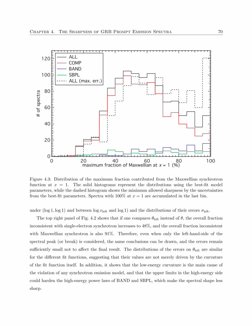
Chapter 4. The Sharpness of GRB Prompt Emission Spectra 70
120
100
80
60
40
20
0
# o
f sp
ectr
a
100806040200maximum fraction of Maxwellian at x = 1 (%)
ALL
COMP
BAND
SBPL
ALL (max. err.)
Figure 4.3: Distribution of the maximum fraction contributed from the Maxwellian synchrotronfunction at x = 1. The solid histograms represent the distributions using the best-fit modelparameters, while the dashed histogram shows the minimum allowed sharpness by the uncertaintiesfrom the best-fit parameters. Spectra with 100% at x = 1 are accumulated in the last bin.
under (log 1, log 1) and between log xleft and log 1) and the distributions of their errors σleft.
The top right panel of Fig. 4.2 shows that if one compares θleft instead of θ, the overall fraction
inconsistent with single-electron synchrotron increases to 48%, and the overall fraction inconsistent
with Maxwellian synchrotron is also 91%. Therefore, even when only the left-hand-side of the
spectral peak (or break) is considered, the same conclusions can be drawn, and the errors remain
sufficiently small not to affect the final result. The distributions of the errors on θleft are similar
for the different fit functions, suggesting that their values are not merely driven by the curvature
of the fit function itself. In addition, it shows that the low-energy curvature is the main cause of
the violation of any synchrotron emission model, and that the upper limits in the high-energy side
could harden the high-energy power laws of BAND and SBPL, which make the spectral shape less
sharp.
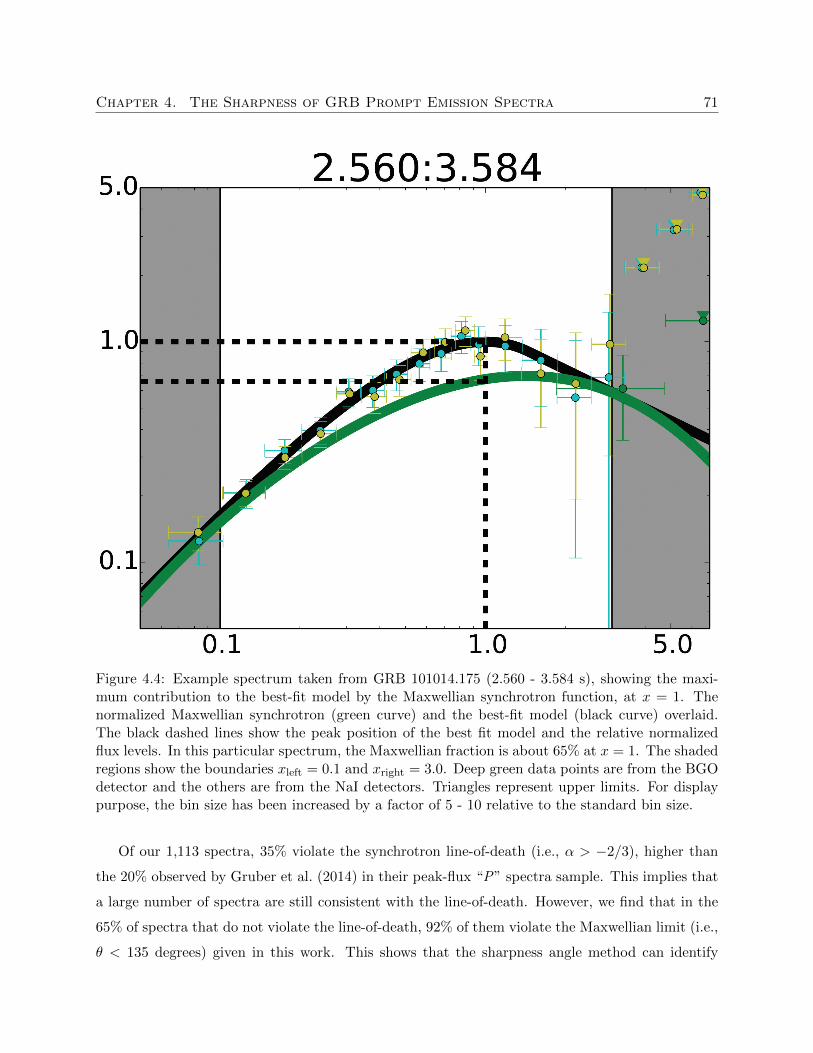
Chapter 4. The Sharpness of GRB Prompt Emission Spectra 71
Figure 4.4: Example spectrum taken from GRB 101014.175 (2.560 - 3.584 s), showing the maxi-mum contribution to the best-fit model by the Maxwellian synchrotron function, at x = 1. Thenormalized Maxwellian synchrotron (green curve) and the best-fit model (black curve) overlaid.The black dashed lines show the peak position of the best fit model and the relative normalizedflux levels. In this particular spectrum, the Maxwellian fraction is about 65% at x = 1. The shadedregions show the boundaries xleft = 0.1 and xright = 3.0. Deep green data points are from the BGOdetector and the others are from the NaI detectors. Triangles represent upper limits. For displaypurpose, the bin size has been increased by a factor of 5 - 10 relative to the standard bin size.
Of our 1,113 spectra, 35% violate the synchrotron line-of-death (i.e., α > −2/3), higher than
the 20% observed by Gruber et al. (2014) in their peak-flux “P” spectra sample. This implies that
a large number of spectra are still consistent with the line-of-death. However, we find that in the
65% of spectra that do not violate the line-of-death, 92% of them violate the Maxwellian limit (i.e.,
θ < 135 degrees) given in this work. This shows that the sharpness angle method can identify
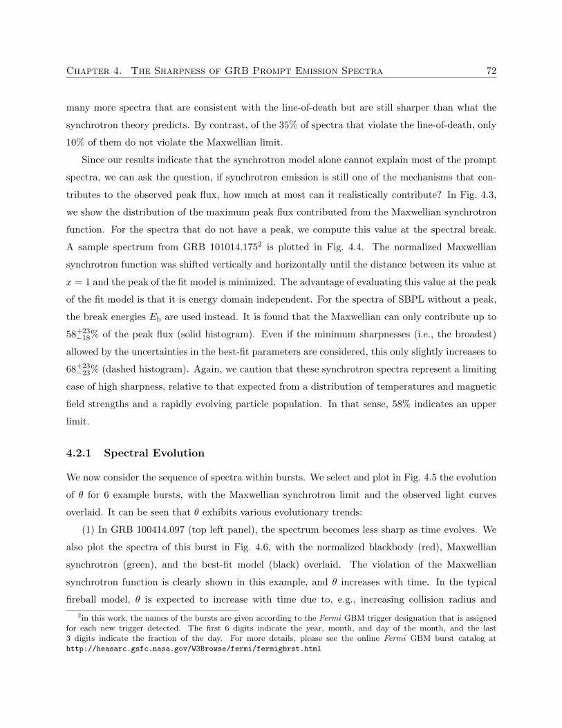
Chapter 4. The Sharpness of GRB Prompt Emission Spectra 72
many more spectra that are consistent with the line-of-death but are still sharper than what the
synchrotron theory predicts. By contrast, of the 35% of spectra that violate the line-of-death, only
10% of them do not violate the Maxwellian limit.
Since our results indicate that the synchrotron model alone cannot explain most of the prompt
spectra, we can ask the question, if synchrotron emission is still one of the mechanisms that con-
tributes to the observed peak flux, how much at most can it realistically contribute? In Fig. 4.3,
we show the distribution of the maximum peak flux contributed from the Maxwellian synchrotron
function. For the spectra that do not have a peak, we compute this value at the spectral break.
A sample spectrum from GRB 101014.1752 is plotted in Fig. 4.4. The normalized Maxwellian
synchrotron function was shifted vertically and horizontally until the distance between its value at
x = 1 and the peak of the fit model is minimized. The advantage of evaluating this value at the peak
of the fit model is that it is energy domain independent. For the spectra of SBPL without a peak,
the break energies Eb are used instead. It is found that the Maxwellian can only contribute up to
58+23−18% of the peak flux (solid histogram). Even if the minimum sharpnesses (i.e., the broadest)
allowed by the uncertainties in the best-fit parameters are considered, this only slightly increases to
68+23−23% (dashed histogram). Again, we caution that these synchrotron spectra represent a limiting
case of high sharpness, relative to that expected from a distribution of temperatures and magnetic
field strengths and a rapidly evolving particle population. In that sense, 58% indicates an upper
limit.
4.2.1 Spectral Evolution
We now consider the sequence of spectra within bursts. We select and plot in Fig. 4.5 the evolution
of θ for 6 example bursts, with the Maxwellian synchrotron limit and the observed light curves
overlaid. It can be seen that θ exhibits various evolutionary trends:
(1) In GRB 100414.097 (top left panel), the spectrum becomes less sharp as time evolves. We
also plot the spectra of this burst in Fig. 4.6, with the normalized blackbody (red), Maxwellian
synchrotron (green), and the best-fit model (black) overlaid. The violation of the Maxwellian
synchrotron function is clearly shown in this example, and θ increases with time. In the typical
fireball model, θ is expected to increase with time due to, e.g., increasing collision radius and
2in this work, the names of the bursts are given according to the Fermi GBM trigger designation that is assignedfor each new trigger detected. The first 6 digits indicate the year, month, and day of the month, and the last3 digits indicate the fraction of the day. For more details, please see the online Fermi GBM burst catalog athttp://heasarc.gsfc.nasa.gov/W3Browse/fermi/fermigbrst.html
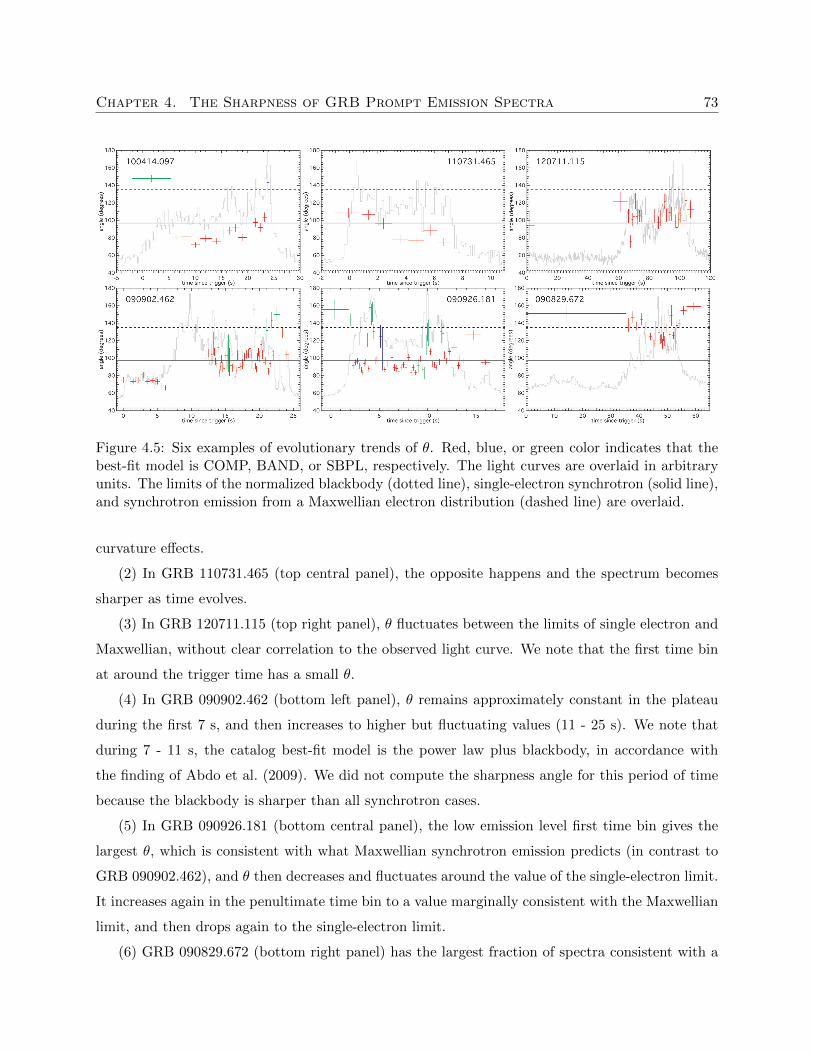
Chapter 4. The Sharpness of GRB Prompt Emission Spectra 73
Figure 4.5: Six examples of evolutionary trends of θ. Red, blue, or green color indicates that thebest-fit model is COMP, BAND, or SBPL, respectively. The light curves are overlaid in arbitraryunits. The limits of the normalized blackbody (dotted line), single-electron synchrotron (solid line),and synchrotron emission from a Maxwellian electron distribution (dashed line) are overlaid.
curvature effects.
(2) In GRB 110731.465 (top central panel), the opposite happens and the spectrum becomes
sharper as time evolves.
(3) In GRB 120711.115 (top right panel), θ fluctuates between the limits of single electron and
Maxwellian, without clear correlation to the observed light curve. We note that the first time bin
at around the trigger time has a small θ.
(4) In GRB 090902.462 (bottom left panel), θ remains approximately constant in the plateau
during the first 7 s, and then increases to higher but fluctuating values (11 - 25 s). We note that
during 7 - 11 s, the catalog best-fit model is the power law plus blackbody, in accordance with
the finding of Abdo et al. (2009). We did not compute the sharpness angle for this period of time
because the blackbody is sharper than all synchrotron cases.
(5) In GRB 090926.181 (bottom central panel), the low emission level first time bin gives the
largest θ, which is consistent with what Maxwellian synchrotron emission predicts (in contrast to
GRB 090902.462), and θ then decreases and fluctuates around the value of the single-electron limit.
It increases again in the penultimate time bin to a value marginally consistent with the Maxwellian
limit, and then drops again to the single-electron limit.
(6) GRB 090829.672 (bottom right panel) has the largest fraction of spectra consistent with a
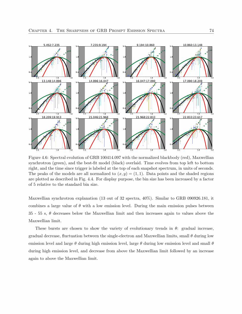
Chapter 4. The Sharpness of GRB Prompt Emission Spectra 74
Figure 4.6: Spectral evolution of GRB 100414.097 with the normalized blackbody (red), Maxwelliansynchrotron (green), and the best-fit model (black) overlaid. Time evolves from top left to bottomright, and the time since trigger is labeled at the top of each snapshot spectrum, in units of seconds.The peaks of the models are all normalized to (x, y) = (1, 1). Data points and the shaded regionsare plotted as described in Fig. 4.4. For display purpose, the bin size has been increased by a factorof 5 relative to the standard bin size.
Maxwellian synchrotron explanation (13 out of 32 spectra, 40%). Similar to GRB 090926.181, it
combines a large value of θ with a low emission level. During the main emission pulses between
35 - 55 s, θ decreases below the Maxwellian limit and then increases again to values above the
Maxwellian limit.
These bursts are chosen to show the variety of evolutionary trends in θ: gradual increase,
gradual decrease, fluctuation between the single-electron and Maxwellian limits, small θ during low
emission level and large θ during high emission level, large θ during low emission level and small θ
during high emission level, and decrease from above the Maxwellian limit followed by an increase
again to above the Maxwellian limit.
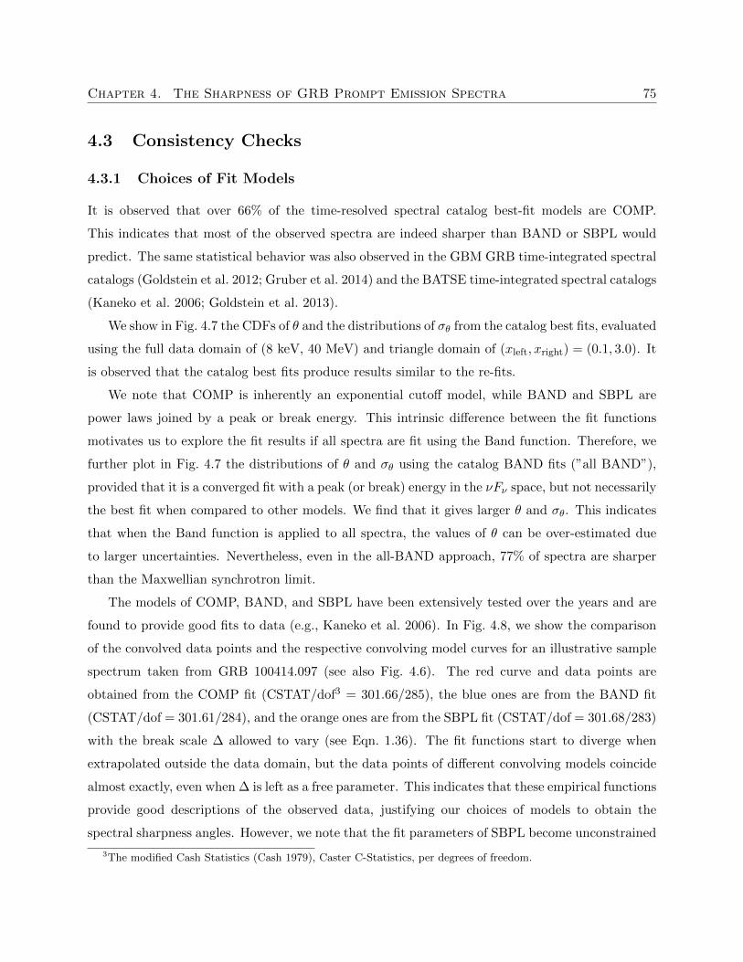
Chapter 4. The Sharpness of GRB Prompt Emission Spectra 75
4.3 Consistency Checks
4.3.1 Choices of Fit Models
It is observed that over 66% of the time-resolved spectral catalog best-fit models are COMP.
This indicates that most of the observed spectra are indeed sharper than BAND or SBPL would
predict. The same statistical behavior was also observed in the GBM GRB time-integrated spectral
catalogs (Goldstein et al. 2012; Gruber et al. 2014) and the BATSE time-integrated spectral catalogs
(Kaneko et al. 2006; Goldstein et al. 2013).
We show in Fig. 4.7 the CDFs of θ and the distributions of σθ from the catalog best fits, evaluated
using the full data domain of (8 keV, 40 MeV) and triangle domain of (xleft, xright) = (0.1, 3.0). It
is observed that the catalog best fits produce results similar to the re-fits.
We note that COMP is inherently an exponential cutoff model, while BAND and SBPL are
power laws joined by a peak or break energy. This intrinsic difference between the fit functions
motivates us to explore the fit results if all spectra are fit using the Band function. Therefore, we
further plot in Fig. 4.7 the distributions of θ and σθ using the catalog BAND fits (”all BAND”),
provided that it is a converged fit with a peak (or break) energy in the νFν space, but not necessarily
the best fit when compared to other models. We find that it gives larger θ and σθ. This indicates
that when the Band function is applied to all spectra, the values of θ can be over-estimated due
to larger uncertainties. Nevertheless, even in the all-BAND approach, 77% of spectra are sharper
than the Maxwellian synchrotron limit.
The models of COMP, BAND, and SBPL have been extensively tested over the years and are
found to provide good fits to data (e.g., Kaneko et al. 2006). In Fig. 4.8, we show the comparison
of the convolved data points and the respective convolving model curves for an illustrative sample
spectrum taken from GRB 100414.097 (see also Fig. 4.6). The red curve and data points are
obtained from the COMP fit (CSTAT/dof3 = 301.66/285), the blue ones are from the BAND fit
(CSTAT/dof = 301.61/284), and the orange ones are from the SBPL fit (CSTAT/dof = 301.68/283)
with the break scale ∆ allowed to vary (see Eqn. 1.36). The fit functions start to diverge when
extrapolated outside the data domain, but the data points of different convolving models coincide
almost exactly, even when ∆ is left as a free parameter. This indicates that these empirical functions
provide good descriptions of the observed data, justifying our choices of models to obtain the
spectral sharpness angles. However, we note that the fit parameters of SBPL become unconstrained
3The modified Cash Statistics (Cash 1979), Caster C-Statistics, per degrees of freedom.
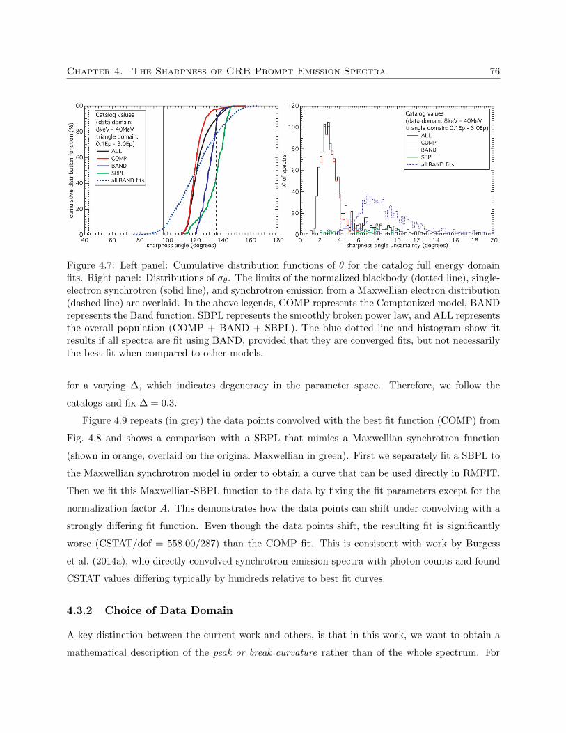
Chapter 4. The Sharpness of GRB Prompt Emission Spectra 76
Figure 4.7: Left panel: Cumulative distribution functions of θ for the catalog full energy domainfits. Right panel: Distributions of σθ. The limits of the normalized blackbody (dotted line), single-electron synchrotron (solid line), and synchrotron emission from a Maxwellian electron distribution(dashed line) are overlaid. In the above legends, COMP represents the Comptonized model, BANDrepresents the Band function, SBPL represents the smoothly broken power law, and ALL representsthe overall population (COMP + BAND + SBPL). The blue dotted line and histogram show fitresults if all spectra are fit using BAND, provided that they are converged fits, but not necessarilythe best fit when compared to other models.
for a varying ∆, which indicates degeneracy in the parameter space. Therefore, we follow the
catalogs and fix ∆ = 0.3.
Figure 4.9 repeats (in grey) the data points convolved with the best fit function (COMP) from
Fig. 4.8 and shows a comparison with a SBPL that mimics a Maxwellian synchrotron function
(shown in orange, overlaid on the original Maxwellian in green). First we separately fit a SBPL to
the Maxwellian synchrotron model in order to obtain a curve that can be used directly in RMFIT.
Then we fit this Maxwellian-SBPL function to the data by fixing the fit parameters except for the
normalization factor A. This demonstrates how the data points can shift under convolving with a
strongly differing fit function. Even though the data points shift, the resulting fit is significantly
worse (CSTAT/dof = 558.00/287) than the COMP fit. This is consistent with work by Burgess
et al. (2014a), who directly convolved synchrotron emission spectra with photon counts and found
CSTAT values differing typically by hundreds relative to best fit curves.
4.3.2 Choice of Data Domain
A key distinction between the current work and others, is that in this work, we want to obtain a
mathematical description of the peak or break curvature rather than of the whole spectrum. For
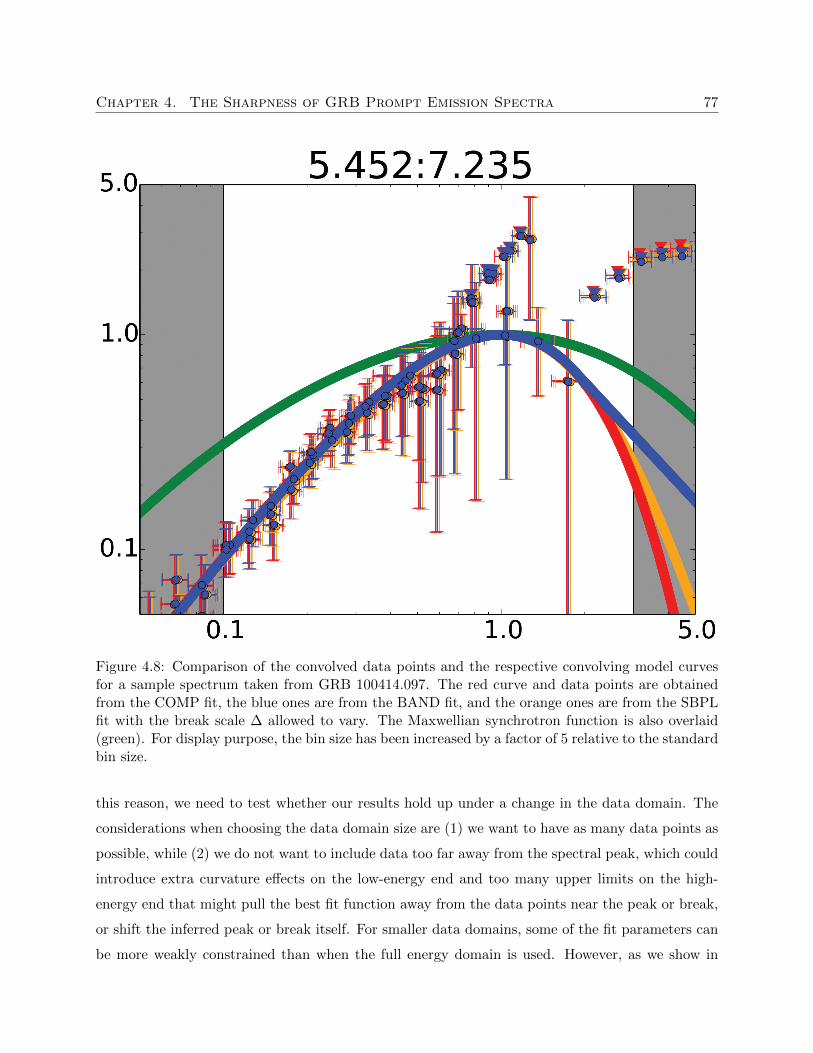
Chapter 4. The Sharpness of GRB Prompt Emission Spectra 77
Figure 4.8: Comparison of the convolved data points and the respective convolving model curvesfor a sample spectrum taken from GRB 100414.097. The red curve and data points are obtainedfrom the COMP fit, the blue ones are from the BAND fit, and the orange ones are from the SBPLfit with the break scale ∆ allowed to vary. The Maxwellian synchrotron function is also overlaid(green). For display purpose, the bin size has been increased by a factor of 5 relative to the standardbin size.
this reason, we need to test whether our results hold up under a change in the data domain. The
considerations when choosing the data domain size are (1) we want to have as many data points as
possible, while (2) we do not want to include data too far away from the spectral peak, which could
introduce extra curvature effects on the low-energy end and too many upper limits on the high-
energy end that might pull the best fit function away from the data points near the peak or break,
or shift the inferred peak or break itself. For smaller data domains, some of the fit parameters can
be more weakly constrained than when the full energy domain is used. However, as we show in
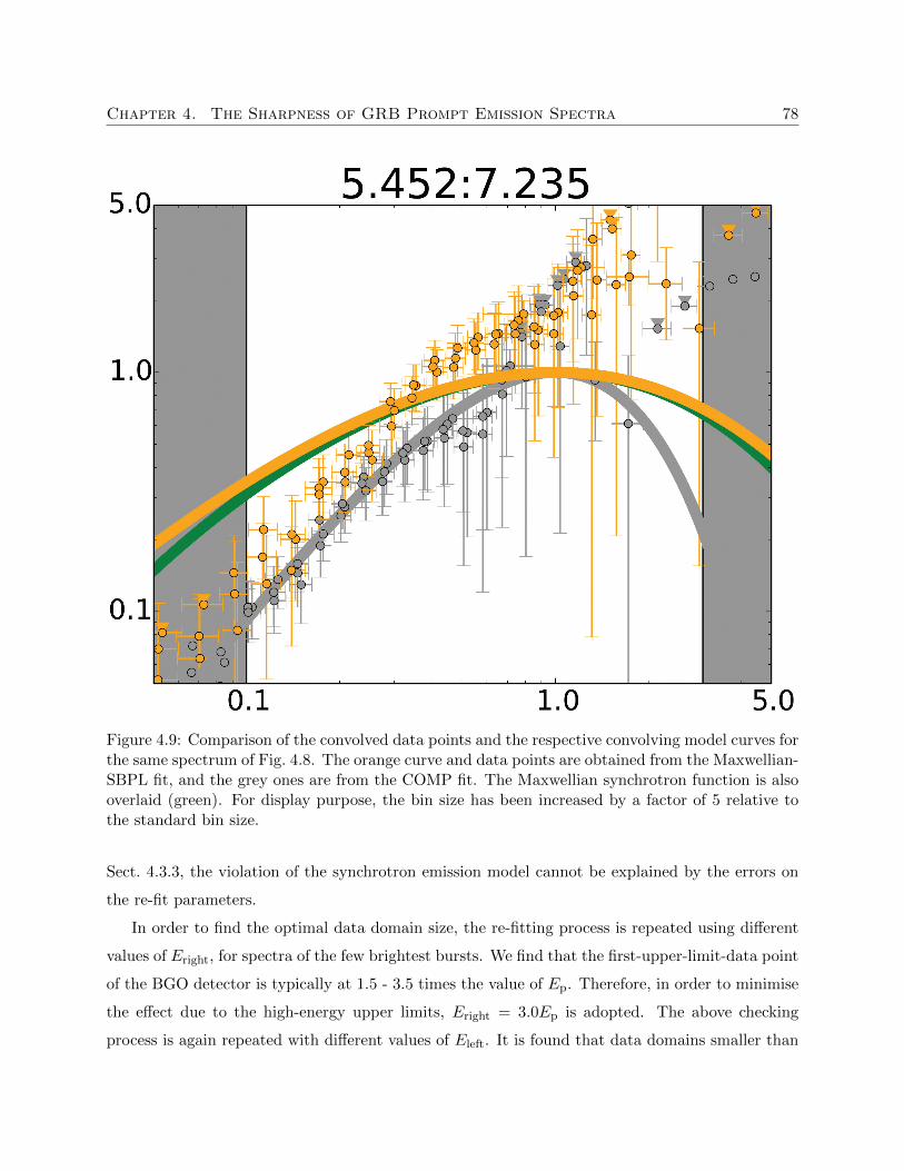
Chapter 4. The Sharpness of GRB Prompt Emission Spectra 78
Figure 4.9: Comparison of the convolved data points and the respective convolving model curves forthe same spectrum of Fig. 4.8. The orange curve and data points are obtained from the Maxwellian-SBPL fit, and the grey ones are from the COMP fit. The Maxwellian synchrotron function is alsooverlaid (green). For display purpose, the bin size has been increased by a factor of 5 relative tothe standard bin size.
Sect. 4.3.3, the violation of the synchrotron emission model cannot be explained by the errors on
the re-fit parameters.
In order to find the optimal data domain size, the re-fitting process is repeated using different
values of Eright, for spectra of the few brightest bursts. We find that the first-upper-limit-data point
of the BGO detector is typically at 1.5 - 3.5 times the value of Ep. Therefore, in order to minimise
the effect due to the high-energy upper limits, Eright = 3.0Ep is adopted. The above checking
process is again repeated with different values of Eleft. It is found that data domains smaller than
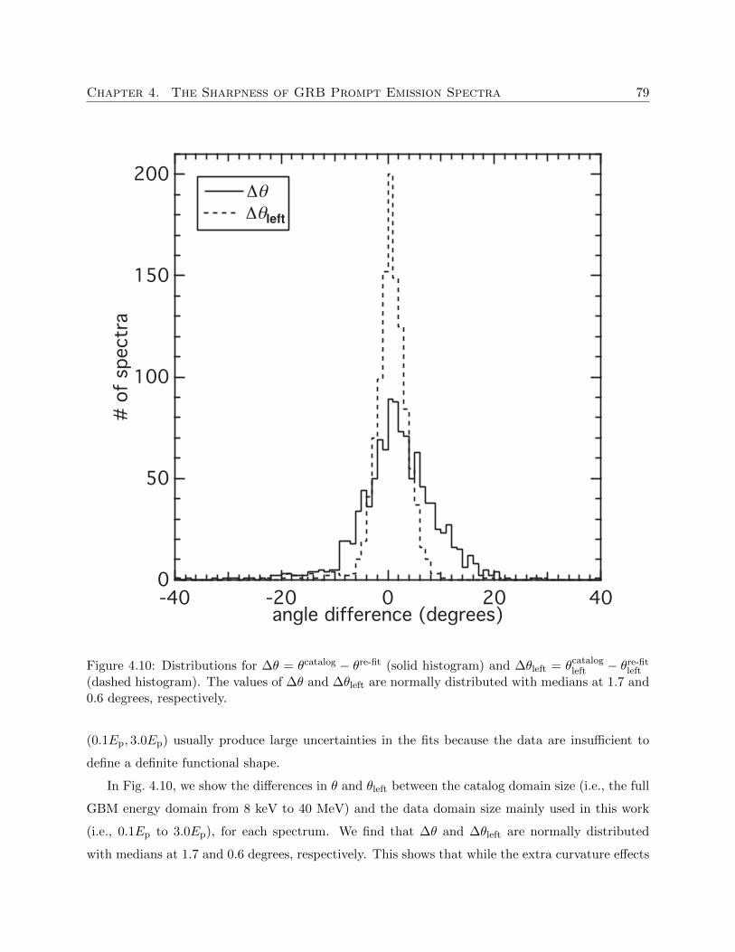
Chapter 4. The Sharpness of GRB Prompt Emission Spectra 79
200
150
100
50
0
# o
f sp
ectr
a
-40 -20 0 20 40angle difference (degrees)
Dq
Dqleft
Figure 4.10: Distributions for ∆θ = θcatalog − θre-fit (solid histogram) and ∆θleft = θcatalogleft − θre-fit
left
(dashed histogram). The values of ∆θ and ∆θleft are normally distributed with medians at 1.7 and0.6 degrees, respectively.
(0.1Ep, 3.0Ep) usually produce large uncertainties in the fits because the data are insufficient to
define a definite functional shape.
In Fig. 4.10, we show the differences in θ and θleft between the catalog domain size (i.e., the full
GBM energy domain from 8 keV to 40 MeV) and the data domain size mainly used in this work
(i.e., 0.1Ep to 3.0Ep), for each spectrum. We find that ∆θ and ∆θleft are normally distributed
with medians at 1.7 and 0.6 degrees, respectively. This shows that while the extra curvature effects
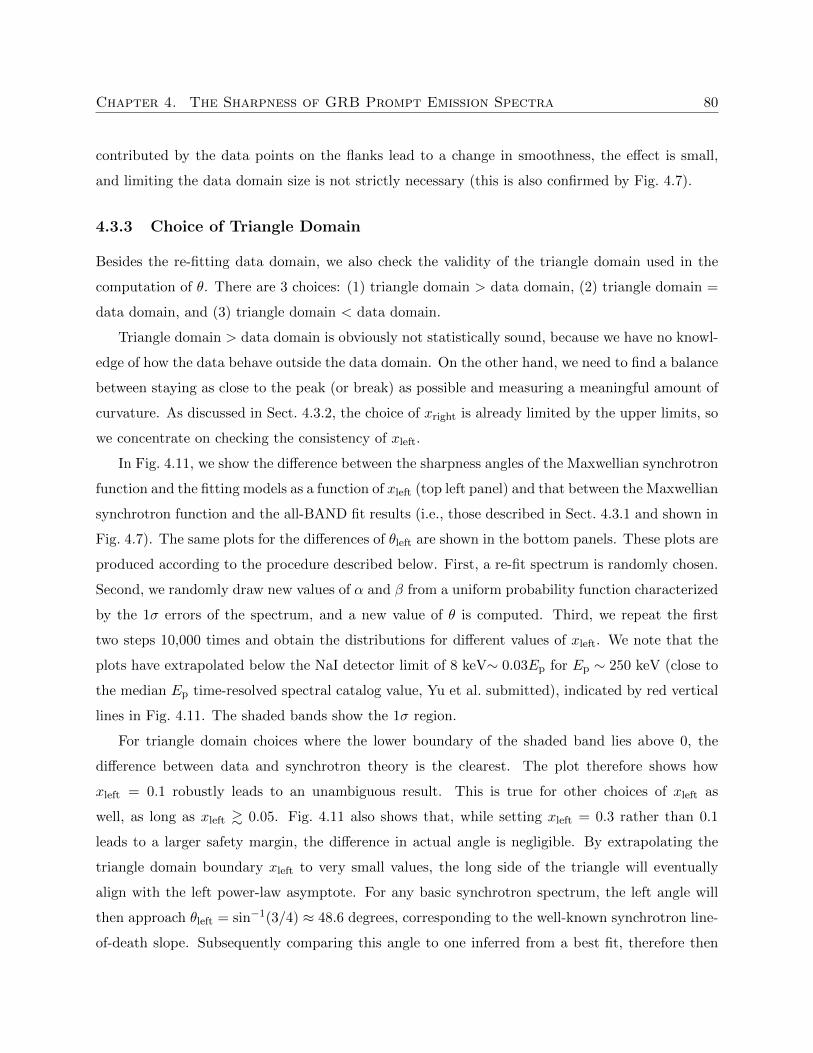
Chapter 4. The Sharpness of GRB Prompt Emission Spectra 80
contributed by the data points on the flanks lead to a change in smoothness, the effect is small,
and limiting the data domain size is not strictly necessary (this is also confirmed by Fig. 4.7).
4.3.3 Choice of Triangle Domain
Besides the re-fitting data domain, we also check the validity of the triangle domain used in the
computation of θ. There are 3 choices: (1) triangle domain > data domain, (2) triangle domain =
data domain, and (3) triangle domain < data domain.
Triangle domain > data domain is obviously not statistically sound, because we have no knowl-
edge of how the data behave outside the data domain. On the other hand, we need to find a balance
between staying as close to the peak (or break) as possible and measuring a meaningful amount of
curvature. As discussed in Sect. 4.3.2, the choice of xright is already limited by the upper limits, so
we concentrate on checking the consistency of xleft.
In Fig. 4.11, we show the difference between the sharpness angles of the Maxwellian synchrotron
function and the fitting models as a function of xleft (top left panel) and that between the Maxwellian
synchrotron function and the all-BAND fit results (i.e., those described in Sect. 4.3.1 and shown in
Fig. 4.7). The same plots for the differences of θleft are shown in the bottom panels. These plots are
produced according to the procedure described below. First, a re-fit spectrum is randomly chosen.
Second, we randomly draw new values of α and β from a uniform probability function characterized
by the 1σ errors of the spectrum, and a new value of θ is computed. Third, we repeat the first
two steps 10,000 times and obtain the distributions for different values of xleft. We note that the
plots have extrapolated below the NaI detector limit of 8 keV∼ 0.03Ep for Ep ∼ 250 keV (close to
the median Ep time-resolved spectral catalog value, Yu et al. submitted), indicated by red vertical
lines in Fig. 4.11. The shaded bands show the 1σ region.
For triangle domain choices where the lower boundary of the shaded band lies above 0, the
difference between data and synchrotron theory is the clearest. The plot therefore shows how
xleft = 0.1 robustly leads to an unambiguous result. This is true for other choices of xleft as
well, as long as xleft & 0.05. Fig. 4.11 also shows that, while setting xleft = 0.3 rather than 0.1
leads to a larger safety margin, the difference in actual angle is negligible. By extrapolating the
triangle domain boundary xleft to very small values, the long side of the triangle will eventually
align with the left power-law asymptote. For any basic synchrotron spectrum, the left angle will
then approach θleft = sin−1(3/4) ≈ 48.6 degrees, corresponding to the well-known synchrotron line-
of-death slope. Subsequently comparing this angle to one inferred from a best fit, therefore then
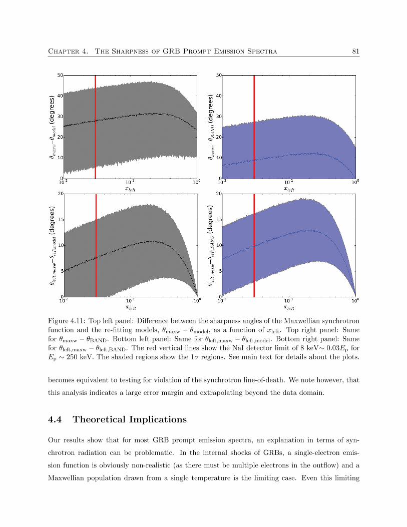
Chapter 4. The Sharpness of GRB Prompt Emission Spectra 81
Figure 4.11: Top left panel: Difference between the sharpness angles of the Maxwellian synchrotronfunction and the re-fitting models, θmaxw − θmodel, as a function of xleft. Top right panel: Samefor θmaxw − θBAND. Bottom left panel: Same for θleft,maxw − θleft,model. Bottom right panel: Samefor θleft,maxw − θleft,BAND. The red vertical lines show the NaI detector limit of 8 keV∼ 0.03Ep forEp ∼ 250 keV. The shaded regions show the 1σ regions. See main text for details about the plots.
becomes equivalent to testing for violation of the synchrotron line-of-death. We note however, that
this analysis indicates a large error margin and extrapolating beyond the data domain.
4.4 Theoretical Implications
Our results show that for most GRB prompt emission spectra, an explanation in terms of syn-
chrotron radiation can be problematic. In the internal shocks of GRBs, a single-electron emis-
sion function is obviously non-realistic (as there must be multiple electrons in the outflow) and a
Maxwellian population drawn from a single temperature is the limiting case. Even this limiting
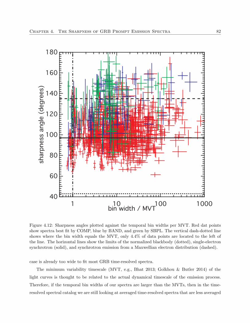
Chapter 4. The Sharpness of GRB Prompt Emission Spectra 82
180
160
140
120
100
80
60
40
sharp
ness
angle
(degre
es)
1 10 100 1000bin width / MVT
Figure 4.12: Sharpness angles plotted against the temporal bin widths per MVT. Red dat pointsshow spectra best fit by COMP, blue by BAND, and green by SBPL. The vertical dash-dotted lineshows where the bin width equals the MVT, only 4.4% of data points are located to the left ofthe line. The horizontal lines show the limits of the normalized blackbody (dotted), single-electronsynchrotron (solid), and synchrotron emission from a Maxwellian electron distribution (dashed).
case is already too wide to fit most GRB time-resolved spectra.
The minimum variability timescale (MVT, e.g., Bhat 2013; Golkhou & Butler 2014) of the
light curves is thought to be related to the actual dynamical timescale of the emission process.
Therefore, if the temporal bin widths of our spectra are larger than the MVTs, then in the time-
resolved spectral catalog we are still looking at averaged time-resolved spectra that are less averaged
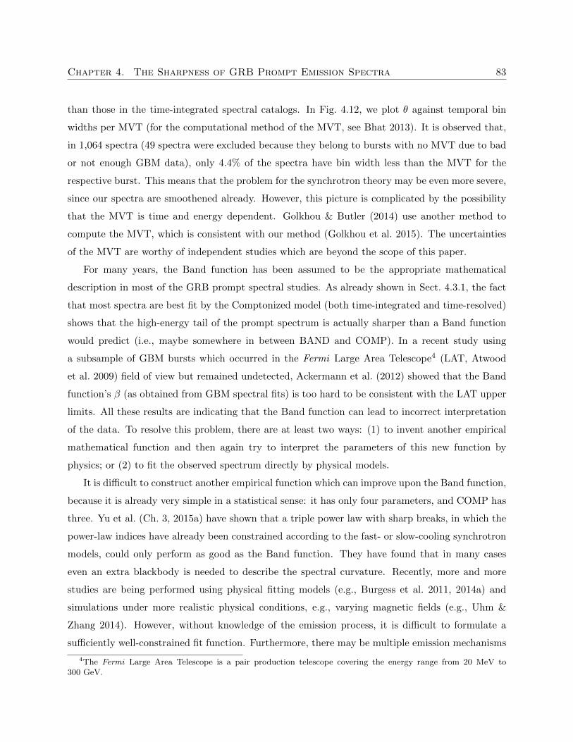
Chapter 4. The Sharpness of GRB Prompt Emission Spectra 83
than those in the time-integrated spectral catalogs. In Fig. 4.12, we plot θ against temporal bin
widths per MVT (for the computational method of the MVT, see Bhat 2013). It is observed that,
in 1,064 spectra (49 spectra were excluded because they belong to bursts with no MVT due to bad
or not enough GBM data), only 4.4% of the spectra have bin width less than the MVT for the
respective burst. This means that the problem for the synchrotron theory may be even more severe,
since our spectra are smoothened already. However, this picture is complicated by the possibility
that the MVT is time and energy dependent. Golkhou & Butler (2014) use another method to
compute the MVT, which is consistent with our method (Golkhou et al. 2015). The uncertainties
of the MVT are worthy of independent studies which are beyond the scope of this paper.
For many years, the Band function has been assumed to be the appropriate mathematical
description in most of the GRB prompt spectral studies. As already shown in Sect. 4.3.1, the fact
that most spectra are best fit by the Comptonized model (both time-integrated and time-resolved)
shows that the high-energy tail of the prompt spectrum is actually sharper than a Band function
would predict (i.e., maybe somewhere in between BAND and COMP). In a recent study using
a subsample of GBM bursts which occurred in the Fermi Large Area Telescope4 (LAT, Atwood
et al. 2009) field of view but remained undetected, Ackermann et al. (2012) showed that the Band
function’s β (as obtained from GBM spectral fits) is too hard to be consistent with the LAT upper
limits. All these results are indicating that the Band function can lead to incorrect interpretation
of the data. To resolve this problem, there are at least two ways: (1) to invent another empirical
mathematical function and then again try to interpret the parameters of this new function by
physics; or (2) to fit the observed spectrum directly by physical models.
It is difficult to construct another empirical function which can improve upon the Band function,
because it is already very simple in a statistical sense: it has only four parameters, and COMP has
three. Yu et al. (Ch. 3, 2015a) have shown that a triple power law with sharp breaks, in which the
power-law indices have already been constrained according to the fast- or slow-cooling synchrotron
models, could only perform as good as the Band function. They have found that in many cases
even an extra blackbody is needed to describe the spectral curvature. Recently, more and more
studies are being performed using physical fitting models (e.g., Burgess et al. 2011, 2014a) and
simulations under more realistic physical conditions, e.g., varying magnetic fields (e.g., Uhm &
Zhang 2014). However, without knowledge of the emission process, it is difficult to formulate a
sufficiently well-constrained fit function. Furthermore, there may be multiple emission mechanisms
4The Fermi Large Area Telescope is a pair production telescope covering the energy range from 20 MeV to300 GeV.
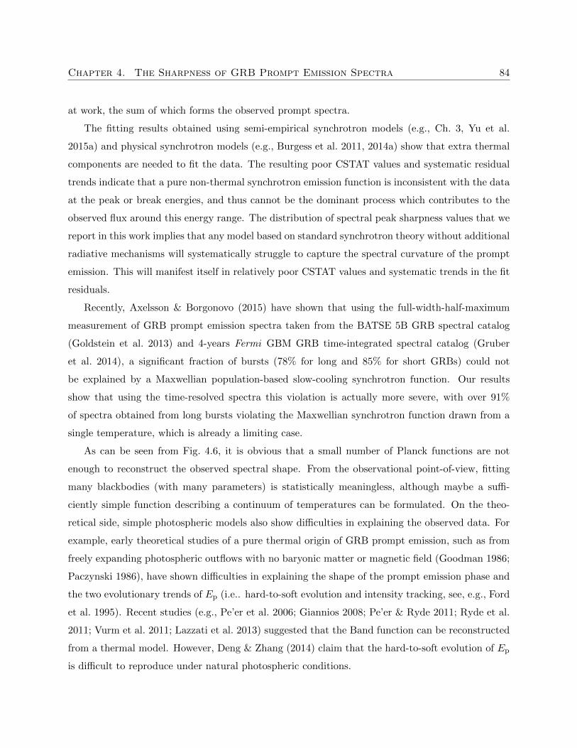
Chapter 4. The Sharpness of GRB Prompt Emission Spectra 84
at work, the sum of which forms the observed prompt spectra.
The fitting results obtained using semi-empirical synchrotron models (e.g., Ch. 3, Yu et al.
2015a) and physical synchrotron models (e.g., Burgess et al. 2011, 2014a) show that extra thermal
components are needed to fit the data. The resulting poor CSTAT values and systematic residual
trends indicate that a pure non-thermal synchrotron emission function is inconsistent with the data
at the peak or break energies, and thus cannot be the dominant process which contributes to the
observed flux around this energy range. The distribution of spectral peak sharpness values that we
report in this work implies that any model based on standard synchrotron theory without additional
radiative mechanisms will systematically struggle to capture the spectral curvature of the prompt
emission. This will manifest itself in relatively poor CSTAT values and systematic trends in the fit
residuals.
Recently, Axelsson & Borgonovo (2015) have shown that using the full-width-half-maximum
measurement of GRB prompt emission spectra taken from the BATSE 5B GRB spectral catalog
(Goldstein et al. 2013) and 4-years Fermi GBM GRB time-integrated spectral catalog (Gruber
et al. 2014), a significant fraction of bursts (78% for long and 85% for short GRBs) could not
be explained by a Maxwellian population-based slow-cooling synchrotron function. Our results
show that using the time-resolved spectra this violation is actually more severe, with over 91%
of spectra obtained from long bursts violating the Maxwellian synchrotron function drawn from a
single temperature, which is already a limiting case.
As can be seen from Fig. 4.6, it is obvious that a small number of Planck functions are not
enough to reconstruct the observed spectral shape. From the observational point-of-view, fitting
many blackbodies (with many parameters) is statistically meaningless, although maybe a suffi-
ciently simple function describing a continuum of temperatures can be formulated. On the theo-
retical side, simple photospheric models also show difficulties in explaining the observed data. For
example, early theoretical studies of a pure thermal origin of GRB prompt emission, such as from
freely expanding photospheric outflows with no baryonic matter or magnetic field (Goodman 1986;
Paczynski 1986), have shown difficulties in explaining the shape of the prompt emission phase and
the two evolutionary trends of Ep (i.e.. hard-to-soft evolution and intensity tracking, see, e.g., Ford
et al. 1995). Recent studies (e.g., Pe’er et al. 2006; Giannios 2008; Pe’er & Ryde 2011; Ryde et al.
2011; Vurm et al. 2011; Lazzati et al. 2013) suggested that the Band function can be reconstructed
from a thermal model. However, Deng & Zhang (2014) claim that the hard-to-soft evolution of Ep
is difficult to reproduce under natural photospheric conditions.
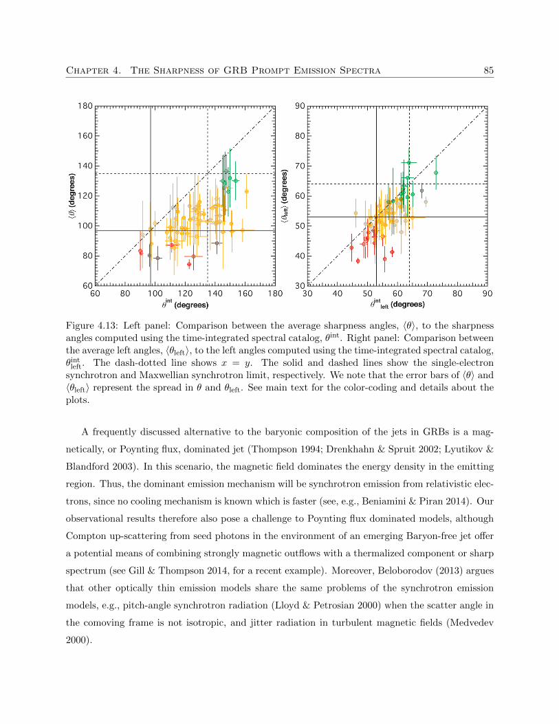
Chapter 4. The Sharpness of GRB Prompt Emission Spectra 85
Figure 4.13: Left panel: Comparison between the average sharpness angles, 〈θ〉, to the sharpnessangles computed using the time-integrated spectral catalog, θint. Right panel: Comparison betweenthe average left angles, 〈θleft〉, to the left angles computed using the time-integrated spectral catalog,θint
left. The dash-dotted line shows x = y. The solid and dashed lines show the single-electronsynchrotron and Maxwellian synchrotron limit, respectively. We note that the error bars of 〈θ〉 and〈θleft〉 represent the spread in θ and θleft. See main text for the color-coding and details about theplots.
A frequently discussed alternative to the baryonic composition of the jets in GRBs is a mag-
netically, or Poynting flux, dominated jet (Thompson 1994; Drenkhahn & Spruit 2002; Lyutikov &
Blandford 2003). In this scenario, the magnetic field dominates the energy density in the emitting
region. Thus, the dominant emission mechanism will be synchrotron emission from relativistic elec-
trons, since no cooling mechanism is known which is faster (see, e.g., Beniamini & Piran 2014). Our
observational results therefore also pose a challenge to Poynting flux dominated models, although
Compton up-scattering from seed photons in the environment of an emerging Baryon-free jet offer
a potential means of combining strongly magnetic outflows with a thermalized component or sharp
spectrum (see Gill & Thompson 2014, for a recent example). Moreover, Beloborodov (2013) argues
that other optically thin emission models share the same problems of the synchrotron emission
models, e.g., pitch-angle synchrotron radiation (Lloyd & Petrosian 2000) when the scatter angle in
the comoving frame is not isotropic, and jitter radiation in turbulent magnetic fields (Medvedev
2000).
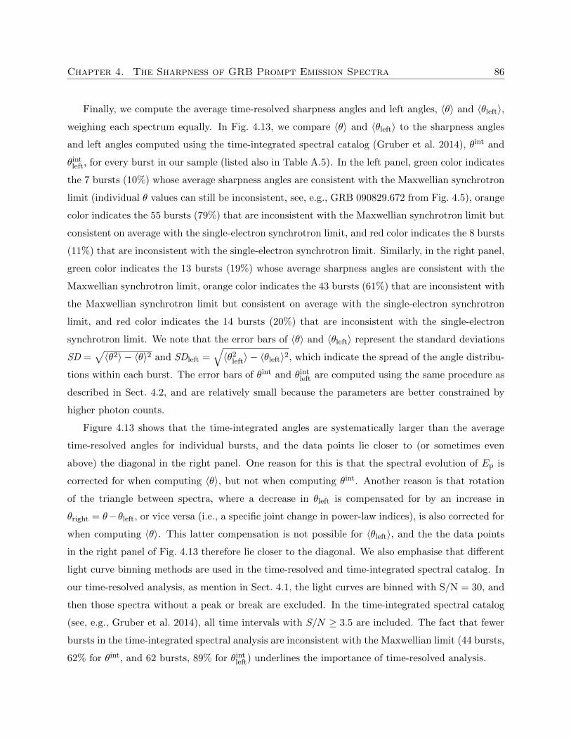
Chapter 4. The Sharpness of GRB Prompt Emission Spectra 86
Finally, we compute the average time-resolved sharpness angles and left angles, 〈θ〉 and 〈θleft〉,
weighing each spectrum equally. In Fig. 4.13, we compare 〈θ〉 and 〈θleft〉 to the sharpness angles
and left angles computed using the time-integrated spectral catalog (Gruber et al. 2014), θint and
θintleft, for every burst in our sample (listed also in Table A.5). In the left panel, green color indicates
the 7 bursts (10%) whose average sharpness angles are consistent with the Maxwellian synchrotron
limit (individual θ values can still be inconsistent, see, e.g., GRB 090829.672 from Fig. 4.5), orange
color indicates the 55 bursts (79%) that are inconsistent with the Maxwellian synchrotron limit but
consistent on average with the single-electron synchrotron limit, and red color indicates the 8 bursts
(11%) that are inconsistent with the single-electron synchrotron limit. Similarly, in the right panel,
green color indicates the 13 bursts (19%) whose average sharpness angles are consistent with the
Maxwellian synchrotron limit, orange color indicates the 43 bursts (61%) that are inconsistent with
the Maxwellian synchrotron limit but consistent on average with the single-electron synchrotron
limit, and red color indicates the 14 bursts (20%) that are inconsistent with the single-electron
synchrotron limit. We note that the error bars of 〈θ〉 and 〈θleft〉 represent the standard deviations
SD =√〈θ2〉 − 〈θ〉2 and SDleft =
√〈θ2
left〉 − 〈θleft〉2, which indicate the spread of the angle distribu-
tions within each burst. The error bars of θint and θintleft are computed using the same procedure as
described in Sect. 4.2, and are relatively small because the parameters are better constrained by
higher photon counts.
Figure 4.13 shows that the time-integrated angles are systematically larger than the average
time-resolved angles for individual bursts, and the data points lie closer to (or sometimes even
above) the diagonal in the right panel. One reason for this is that the spectral evolution of Ep is
corrected for when computing 〈θ〉, but not when computing θint. Another reason is that rotation
of the triangle between spectra, where a decrease in θleft is compensated for by an increase in
θright = θ−θleft, or vice versa (i.e., a specific joint change in power-law indices), is also corrected for
when computing 〈θ〉. This latter compensation is not possible for 〈θleft〉, and the the data points
in the right panel of Fig. 4.13 therefore lie closer to the diagonal. We also emphasise that different
light curve binning methods are used in the time-resolved and time-integrated spectral catalog. In
our time-resolved analysis, as mention in Sect. 4.1, the light curves are binned with S/N = 30, and
then those spectra without a peak or break are excluded. In the time-integrated spectral catalog
(see, e.g., Gruber et al. 2014), all time intervals with S/N ≥ 3.5 are included. The fact that fewer
bursts in the time-integrated spectral analysis are inconsistent with the Maxwellian limit (44 bursts,
62% for θint, and 62 bursts, 89% for θintleft) underlines the importance of time-resolved analysis.
Chapter 4. The Sharpness of GRB Prompt Emission Spectra 87
4.5 Conclusions
We have computed the sharpness angles θ of the observed time-resolved spectra of Fermi GRBs,
and compared the values to the sharpest cases of the synchrotron radiation theory, namely the
single-electron synchrotron and the Maxwellian distributed synchrotron emission function. We
find that over 91% of the observed spectra are sharper than the Maxwellian synchrotron model
predicts, indicating that synchrotron radiation cannot be responsible for the peaks or breaks of
GRB prompt emission spectra. No general evolutionary trend is observed for θ within bursts.
Moreover, the Maxwellian synchrotron function can only contribute up to 58+23−18% of the peak
flux. We conclude that the underlying prompt emission mechanism in GRBs must produce spectra
sharper than a Maxwellian synchrotron function but broader than a blackbody.
It is still possible for synchrotron emission to dominate the spectrum away from the peak or
break observed in the GBM energy range (e.g., at the LAT energy range). Also, a sub-dominant
synchrotron component can allow for a continuous connection to the afterglow phase, where syn-
chrotron emission is typically dominant (see, e.g., van Eerten 2015, for a recent review). The tran-
sition between prompt and afterglow is then marked by the disappearance of the non-synchrotron
(likely thermal) component. There are other theoretical possibilities to explain GRB prompt emis-
sion, such as the collisional model of electron-positron pairs (e.g., Beloborodov 2010). For recent
reviews on GRB prompt emission mechanisms, see, e.g., Zhang (2014) and Pe’er (2015).
A possibly similar inference can be made on the related phenomena of prompt optical emission
showing a similar temporal profile as the gamma-ray emission (e.g., Elliott et al. 2014; Greiner
et al. 2014) or very early X-ray flares (e.g., Pe’er et al. 2006; see also Hu et al. 2014 for a recent
large Swift sample study): if the prompt emission is not dominated by synchrotron emission, this
is likely the case for this longer wavelength emission as well (see, e.g., Starling et al. 2012; Peng
et al. 2014).
We demonstrated in this work a method to quantify the shape of the observed GRB spectra that
provides a clear tool for distinguishing between various standard emission functions. Ultimately, the
question as to the viability of any particular emission model can only be fully resolved if complete
spectral predictions for that model are tested directly against photon counts (see, e.g., Burgess
et al. 2014a). Our paper predicts that any model based on standard synchrotron theory without
additional radiative mechanisms will systematically struggle to capture the spectral curvature of
the prompt emission. This will manifest itself in relatively poor CSTAT values and trends in the
fit residuals.
Chapter 5
Summary and Future Directions
“It is scientific only to say what is more likely and
what less likely, and not to be proving all the time
the possible and impossible.”
- Richard Feynman
In this dissertation, I presented time-resolved spectroscopy on GRB prompt emission spectra.
The analysis results indicate that optically thin synchrotron emission is very unlikely to be the
dominant process in shaping the observed spectral shapes of GRBs, due to the following reasons:
(1) thought some brightest bursts can marginally be explained by a complex empirical
model of thermal + non-thermal emission, fine-tuned microphysics parameters and
varying magnetic fields are required;
(2) the peaks or breaks of more than 91% of time-resolved prompt spectra is sharper
than the sharpest possible pure optically thin synchrotron emission model would pre-
dict.
Some possible solutions, however, do exist. For instance a simple enough summation of black-
bodies (a “greybody”), absorbed synchrotron (i.e., optically thick), pitch-angle synchrotron, jitter
radiation, or collisional processes may be formulated to fit the data. Consequently, the answer to
“What is the true emission mechanism of GRB prompt emission?” is still unclear. This is very
true in science: falsifying is often easier than validating a hypothesis. Several research directions
are foreseeable in the near future. On one hand, “hard science” like to build the next generation of
gamma-ray space telescopes with unprecedented precision and resolution is of course necessary to
88
Chapter 5. Summary and Future Directions 89
constraint theoretical models. On the other hand, “soft science” like to analyze existing data using
advanced numerical methods can also help to pin-down the true emission mechanism of GRBs, e.g.,
precise background and spectral fitting techniques using physical models.
Gamma-ray burst prompt emission mechanism is a very important topic because the emission
process tells us information of, e.g., the environment of the jet and circum-burst medium, and the
nature of the central engine, which can be used to constraint galaxy properties and star formation
history. The hope of using GRBs as standard candles also makes them useful in cosmological
studies.
While the mission direction of the next generation gamma-ray space telescopes is unclear, the
existing data we have in hand are still highly unexplored. The next possible step is to develop an
automated time-resolved spectroscopy pipeline to fit these data using advanced Bayesian statistics.
This should be able to explain the GRB prompt spectra by fitting physical emission models directly
to data, which may lead to a full understanding of these cosmological gamma-ray transients.

Bibliography
Abdo, A. A., Ackermann, M., Ajello, M., et al. 2009, ApJL, 706, L138
Abdo, A. A., Ackermann, M., Ajello, M., et al. 2010, ApJ, 712, 558
Achterberg, A., Gallant, Y. A., Kirk, J. G., & Guthmann, A. W. 2001, MNRAS, 328, 393
Ackermann, M., Ajello, M., Asano, K., et al. 2014, Science, 343, 42
Ackermann, M., Ajello, M., Asano, K., et al. 2013, ApJS, 209, 11
Ackermann, M., Ajello, M., Baldini, L., et al. 2012, ApJ, 754, 121
Akerlof, C., Balsano, R., Barthelmy, S., et al. 2000, ApJL, 532, L25
Amati, L. 2010, arXiv:1002.2232
Amati, L., Frontera, F., Tavani, M., et al. 2002, A&A, 390, 81
Amati, L., Guidorzi, C., Frontera, F., et al. 2008, MNRAS, 391, 577
Atwood, W. B., Abdo, A. A., Ackermann, M., et al. 2009, ApJ, 697, 1071
Axelsson, M., Baldini, L., Barbiellini, G., et al. 2012, ApJL, 757, L31
Axelsson, M. & Borgonovo, L. 2015, MNRAS, 447, 3150
Band, D., Matteson, J., Ford, L., et al. 1993, ApJ, 413, 281
Baring, M. G. 2006, Advances in Space Research, 38, 1281
90
Bibliography 91
Baring, M. G. & Braby, M. L. 2004, ApJ, 613, 460
Barthelmy, S. D. 2000, in Society of Photo-Optical Instrumentation Engineers (SPIE) Conference
Series, Vol. 4140, X-Ray and Gamma-Ray Instrumentation for Astronomy XI, ed. K. A. Flanagan
& O. H. Siegmund, 50–63
Barthelmy, S. D., Barbier, L. M., Cummings, J. R., et al. 2005, Space Sci. Rev., 120, 143
Bednarz, J. & Ostrowski, M. 1998, Physical Review Letters, 80, 3911
Beloborodov, A. M. 2010, MNRAS, 407, 1033
Beloborodov, A. M. 2011, ApJ, 737, 68
Beloborodov, A. M. 2013, ApJ, 764, 157
Beniamini, P. & Piran, T. 2014, MNRAS, 445, 3892
Bhat, P. N. 2013, in ”Proc. 7th Huntsville GRB Symp.”, Huntsville, Apr. 2013, eConf Proc.
C1304143
Bissaldi, E., von Kienlin, A., Kouveliotou, C., et al. 2011, ApJ, 733, 97
Bissaldi, E., von Kienlin, A., Lichti, G., et al. 2009, Experimental Astronomy, 24, 47
Blumenthal, G. R. & Gould, R. J. 1970, Reviews of Modern Physics, 42, 237
Boella, G., Butler, R. C., Perola, G. C., et al. 1997, A&As, 122, 299
Briggs, M. S., Paciesas, W. S., Pendleton, G. N., et al. 1996, ApJ, 459, 40
Burgess, J. M., Preece, R. D., Baring, M. G., et al. 2011, ApJ, 741, 24
Burgess, J. M., Preece, R. D., Connaughton, V., et al. 2014a, ApJ, 784, 17
Burgess, J. M., Preece, R. D., Ryde, F., et al. 2014b, ApJL, 784, L43
Burgess, J. M., Ryde, F., & Yu, H.-F. 2015, MNRAS, 451, 6029
Burrows, D. N., Hill, J. E., Nousek, J. A., et al. 2000, in Society of Photo-Optical Instrumentation
Engineers (SPIE) Conference Series, Vol. 4140, X-Ray and Gamma-Ray Instrumentation for
Astronomy XI, ed. K. A. Flanagan & O. H. Siegmund, 64–75
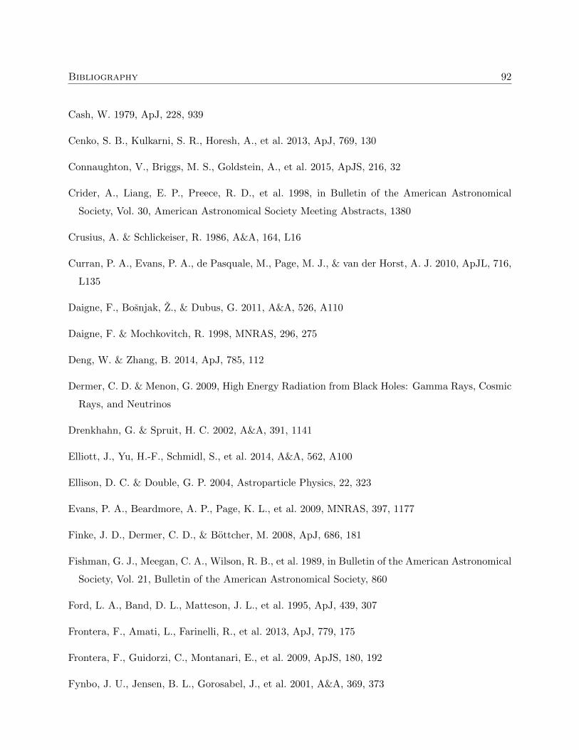
Bibliography 92
Cash, W. 1979, ApJ, 228, 939
Cenko, S. B., Kulkarni, S. R., Horesh, A., et al. 2013, ApJ, 769, 130
Connaughton, V., Briggs, M. S., Goldstein, A., et al. 2015, ApJS, 216, 32
Crider, A., Liang, E. P., Preece, R. D., et al. 1998, in Bulletin of the American Astronomical
Society, Vol. 30, American Astronomical Society Meeting Abstracts, 1380
Crusius, A. & Schlickeiser, R. 1986, A&A, 164, L16
Curran, P. A., Evans, P. A., de Pasquale, M., Page, M. J., & van der Horst, A. J. 2010, ApJL, 716,
L135
Daigne, F., Bosnjak, Z., & Dubus, G. 2011, A&A, 526, A110
Daigne, F. & Mochkovitch, R. 1998, MNRAS, 296, 275
Deng, W. & Zhang, B. 2014, ApJ, 785, 112
Dermer, C. D. & Menon, G. 2009, High Energy Radiation from Black Holes: Gamma Rays, Cosmic
Rays, and Neutrinos
Drenkhahn, G. & Spruit, H. C. 2002, A&A, 391, 1141
Elliott, J., Yu, H.-F., Schmidl, S., et al. 2014, A&A, 562, A100
Ellison, D. C. & Double, G. P. 2004, Astroparticle Physics, 22, 323
Evans, P. A., Beardmore, A. P., Page, K. L., et al. 2009, MNRAS, 397, 1177
Finke, J. D., Dermer, C. D., & Bottcher, M. 2008, ApJ, 686, 181
Fishman, G. J., Meegan, C. A., Wilson, R. B., et al. 1989, in Bulletin of the American Astronomical
Society, Vol. 21, Bulletin of the American Astronomical Society, 860
Ford, L. A., Band, D. L., Matteson, J. L., et al. 1995, ApJ, 439, 307
Frontera, F., Amati, L., Farinelli, R., et al. 2013, ApJ, 779, 175
Frontera, F., Guidorzi, C., Montanari, E., et al. 2009, ApJS, 180, 192
Fynbo, J. U., Jensen, B. L., Gorosabel, J., et al. 2001, A&A, 369, 373
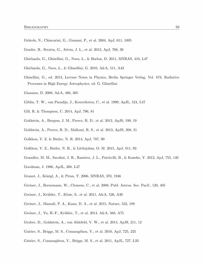
Bibliography 93
Gehrels, N., Chincarini, G., Giommi, P., et al. 2004, ApJ, 611, 1005
Gendre, B., Stratta, G., Atteia, J. L., et al. 2013, ApJ, 766, 30
Ghirlanda, G., Ghisellini, G., Nava, L., & Burlon, D. 2011, MNRAS, 410, L47
Ghirlanda, G., Nava, L., & Ghisellini, G. 2010, A&A, 511, A43
Ghisellini, G., ed. 2013, Lecture Notes in Physics, Berlin Springer Verlag, Vol. 873, Radiative
Processes in High Energy Astrophysics, ed. G. Ghisellini
Giannios, D. 2008, A&A, 480, 305
Giblin, T. W., van Paradijs, J., Kouveliotou, C., et al. 1999, ApJL, 524, L47
Gill, R. & Thompson, C. 2014, ApJ, 796, 81
Goldstein, A., Burgess, J. M., Preece, R. D., et al. 2012, ApJS, 199, 19
Goldstein, A., Preece, R. D., Mallozzi, R. S., et al. 2013, ApJS, 208, 21
Golkhou, V. Z. & Butler, N. R. 2014, ApJ, 787, 90
Golkhou, V. Z., Butler, N. R., & Littlejohns, O. M. 2015, ApJ, 811, 93
Gonzalez, M. M., Sacahui, J. R., Ramirez, J. L., Patricelli, B., & Kaneko, Y. 2012, ApJ, 755, 140
Goodman, J. 1986, ApJL, 308, L47
Granot, J., Konigl, A., & Piran, T. 2006, MNRAS, 370, 1946
Greiner, J., Bornemann, W., Clemens, C., et al. 2008, Publ. Astron. Soc. Pacif., 120, 405
Greiner, J., Kruhler, T., Klose, S., et al. 2011, A&A, 526, A30
Greiner, J., Mazzali, P. A., Kann, D. A., et al. 2015, Nature, 523, 189
Greiner, J., Yu, H.-F., Kruhler, T., et al. 2014, A&A, 568, A75
Gruber, D., Goldstein, A., von Ahlefeld, V. W., et al. 2014, ApJS, 211, 12
Guiriec, S., Briggs, M. S., Connaugthon, V., et al. 2010, ApJ, 725, 225
Guiriec, S., Connaughton, V., Briggs, M. S., et al. 2011, ApJL, 727, L33
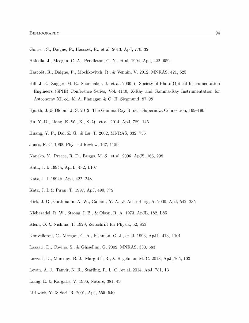
Bibliography 94
Guiriec, S., Daigne, F., Hascoet, R., et al. 2013, ApJ, 770, 32
Hakkila, J., Meegan, C. A., Pendleton, G. N., et al. 1994, ApJ, 422, 659
Hascoet, R., Daigne, F., Mochkovitch, R., & Vennin, V. 2012, MNRAS, 421, 525
Hill, J. E., Zugger, M. E., Shoemaker, J., et al. 2000, in Society of Photo-Optical Instrumentation
Engineers (SPIE) Conference Series, Vol. 4140, X-Ray and Gamma-Ray Instrumentation for
Astronomy XI, ed. K. A. Flanagan & O. H. Siegmund, 87–98
Hjorth, J. & Bloom, J. S. 2012, The Gamma-Ray Burst - Supernova Connection, 169–190
Hu, Y.-D., Liang, E.-W., Xi, S.-Q., et al. 2014, ApJ, 789, 145
Huang, Y. F., Dai, Z. G., & Lu, T. 2002, MNRAS, 332, 735
Jones, F. C. 1968, Physical Review, 167, 1159
Kaneko, Y., Preece, R. D., Briggs, M. S., et al. 2006, ApJS, 166, 298
Katz, J. I. 1994a, ApJL, 432, L107
Katz, J. I. 1994b, ApJ, 422, 248
Katz, J. I. & Piran, T. 1997, ApJ, 490, 772
Kirk, J. G., Guthmann, A. W., Gallant, Y. A., & Achterberg, A. 2000, ApJ, 542, 235
Klebesadel, R. W., Strong, I. B., & Olson, R. A. 1973, ApJL, 182, L85
Klein, O. & Nishina, T. 1929, Zeitschrift fur Physik, 52, 853
Kouveliotou, C., Meegan, C. A., Fishman, G. J., et al. 1993, ApJL, 413, L101
Lazzati, D., Covino, S., & Ghisellini, G. 2002, MNRAS, 330, 583
Lazzati, D., Morsony, B. J., Margutti, R., & Begelman, M. C. 2013, ApJ, 765, 103
Levan, A. J., Tanvir, N. R., Starling, R. L. C., et al. 2014, ApJ, 781, 13
Liang, E. & Kargatis, V. 1996, Nature, 381, 49
Lithwick, Y. & Sari, R. 2001, ApJ, 555, 540
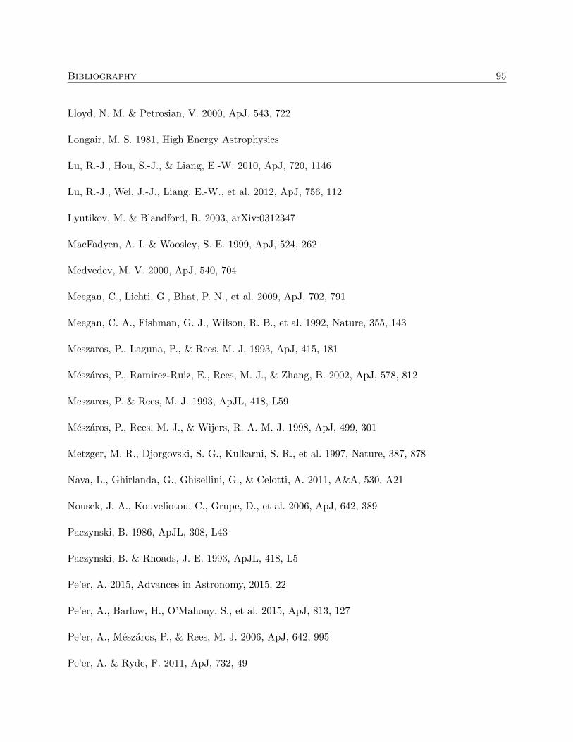
Bibliography 95
Lloyd, N. M. & Petrosian, V. 2000, ApJ, 543, 722
Longair, M. S. 1981, High Energy Astrophysics
Lu, R.-J., Hou, S.-J., & Liang, E.-W. 2010, ApJ, 720, 1146
Lu, R.-J., Wei, J.-J., Liang, E.-W., et al. 2012, ApJ, 756, 112
Lyutikov, M. & Blandford, R. 2003, arXiv:0312347
MacFadyen, A. I. & Woosley, S. E. 1999, ApJ, 524, 262
Medvedev, M. V. 2000, ApJ, 540, 704
Meegan, C., Lichti, G., Bhat, P. N., et al. 2009, ApJ, 702, 791
Meegan, C. A., Fishman, G. J., Wilson, R. B., et al. 1992, Nature, 355, 143
Meszaros, P., Laguna, P., & Rees, M. J. 1993, ApJ, 415, 181
Meszaros, P., Ramirez-Ruiz, E., Rees, M. J., & Zhang, B. 2002, ApJ, 578, 812
Meszaros, P. & Rees, M. J. 1993, ApJL, 418, L59
Meszaros, P., Rees, M. J., & Wijers, R. A. M. J. 1998, ApJ, 499, 301
Metzger, M. R., Djorgovski, S. G., Kulkarni, S. R., et al. 1997, Nature, 387, 878
Nava, L., Ghirlanda, G., Ghisellini, G., & Celotti, A. 2011, A&A, 530, A21
Nousek, J. A., Kouveliotou, C., Grupe, D., et al. 2006, ApJ, 642, 389
Paczynski, B. 1986, ApJL, 308, L43
Paczynski, B. & Rhoads, J. E. 1993, ApJL, 418, L5
Pe’er, A. 2015, Advances in Astronomy, 2015, 22
Pe’er, A., Barlow, H., O’Mahony, S., et al. 2015, ApJ, 813, 127
Pe’er, A., Meszaros, P., & Rees, M. J. 2006, ApJ, 642, 995
Pe’er, A. & Ryde, F. 2011, ApJ, 732, 49
Bibliography 96
Pe’er, A., Zhang, B.-B., Ryde, F., et al. 2012, MNRAS, 420, 468
Pendleton, G. N., Paciesas, W. S., Briggs, M. S., et al. 1994, ApJ, 431, 416
Peng, F.-K., Liang, E.-W., Wang, X.-Y., et al. 2014, ApJ, 795, 155
Peng, Z. Y., Yin, Y., Bi, X. W., et al. 2010, ApJ, 718, 894
Piran, T. 1999, Phys. Rep., 314, 575
Piran, T. 2004, Reviews of Modern Physics, 76, 1143
Preece, R., Burgess, J. M., von Kienlin, A., et al. 2014, Science, 343, 51
Preece, R. D., Briggs, M. S., Giblin, T. W., et al. 2002, ApJ, 581, 1248
Preece, R. D., Briggs, M. S., Mallozzi, R. S., et al. 1998a, ApJL, 506, L23
Preece, R. D., Briggs, M. S., Mallozzi, R. S., et al. 2000, ApJS, 126, 19
Preece, R. D., Briggs, M. S., Pendleton, G. N., et al. 1996, ApJ, 473, 310
Preece, R. D., Pendleton, G. N., Briggs, M. S., et al. 1998b, ApJ, 496, 849
Racusin, J. L., Karpov, S. V., Sokolowski, M., et al. 2008, Nature, 455, 183
Rees, M. J. & Meszaros, P. 1992, MNRAS, 258, 41P
Rees, M. J. & Meszaros, P. 1994, ApJL, 430, L93
Rhoads, J. E. 1997, ApJL, 487, L1
Ryan, G., van Eerten, H., MacFadyen, A., & Zhang, B.-B. 2015, ApJ, 799, 3
Rybicki, G. B. & Lightman, A. P. 1979, Radiative Processes in Astrophysics
Ryde, F. 1999, Astrophysical Letters and Communications, 39, 281
Ryde, F. 2005, ApJL, 625, L95
Ryde, F., Pe’er, A., Nymark, T., et al. 2011, MNRAS, 415, 3693
Bibliography 97
Sacahui, J. R., Gonzalez, M. M., Fraija, N., Ramirez, J. L., & Lee, W. H. 2013, in EAS Publications
Series, Vol. 61, EAS Publications Series, ed. A. J. Castro-Tirado, J. Gorosabel, & I. H. Park,
301–305
Sakamoto, T., Barthelmy, S. D., Barbier, L., et al. 2008, ApJS, 175, 179
Sakamoto, T., Barthelmy, S. D., Baumgartner, W. H., et al. 2011, ApJS, 195, 2
Sari, R., Piran, T., & Narayan, R. 1998, ApJL, 497, L17
Spearman, C. 1904, The American Journal of Psychology, 15, 72
Spitkovsky, A. 2008, ApJL, 682, L5
Starling, R. L. C., Page, K. L., Pe’Er, A., Beardmore, A. P., & Osborne, J. P. 2012, MNRAS, 427,
2950
Stratta, G., Gendre, B., Atteia, J. L., et al. 2013, ApJ, 779, 66
Summerlin, E. J. & Baring, M. G. 2012, ApJ, 745, 63
Tanvir, N. R. 2013, arXiv:1307.6156
Tavani, M. 1995, Ap&SS, 231, 181
Tavani, M. 1996, ApJ, 466, 768
Tegmark, M., Hartmann, D. H., Briggs, M. S., & Meegan, C. A. 1996, ApJ, 468, 214
Thompson, C. 1994, MNRAS, 270, 480
Uhm, Z. L. & Zhang, B. 2014, Nature Physics, 10, 351
van den Bergh, S. 1983, Ap. Space Sci., 97, 385
van Eerten, H. J. 2015, Journal of High Energy Astrophysics, 7, 23
van Eerten, H. J. & Wijers, R. A. M. J. 2009, MNRAS, 394, 2164
von Kienlin, A., Meegan, C. A., Paciesas, W. S., et al. 2014, ApJS, 211, 13
Vurm, I. & Beloborodov, A. M. 2015, arXiv:1506.01107
Bibliography 98
Vurm, I., Beloborodov, A. M., & Poutanen, J. 2011, ApJ, 738, 77
Waxman, E. 1997a, ApJL, 485, L5
Waxman, E. 1997b, ApJL, 489, L33
Wijers, R. A. M. J., Rees, M. J., & Meszaros, P. 1997, MNRAS, 288, L51
Woosley, S. E. 1993, ApJ, 405, 273
Woosley, S. E. 1996, in American Institute of Physics Conference Series, Vol. 384, American Insti-
tute of Physics Conference Series, ed. C. Kouveliotou, M. F. Briggs, & G. J. Fishman, 709–718
Yonetoku, D., Murakami, T., Nakamura, T., et al. 2004, ApJ, 609, 935
Yu, H.-F., Greiner, J., van Eerten, H., et al. 2015a, A&A, 573, A81
Yu, H.-F., Preece, R. D., Greiner, J., et al. submitted, A&A
Yu, H.-F., van Eerten, H. J., Greiner, J., et al. 2015b, A&A, 583, A129
Zhang, B. 2014, International Journal of Modern Physics D, 23, 1430002
Zhang, B.-B., Uhm, Z. L., Connaughton, V., Briggs, M. S., & Zhang, B. 2016, ApJ, 816, 72

Acknowledgements
I never believed I would be writing my Ph.D. dissertation here in Garching bei Munchen, Germany.
I was an ordinary kid grown up in an old small town, Sai Ying Pun in Hong Kong. I built up
my passion for physics only during the last two years in secondary school. I remember that day
I randomly read Richard Feynman’s book in a book store, when I didn’t even know who is this
guy. But he changed my life. This guy is so cool, I thought, I wanna be just like him. Of course,
I am not a magician nor a genius like him, but I feel happy and touched every time I think about
physics, and I know this is what I wanna do.
Time flies. Three years have passed since the day we arrived in Munich. Six years since I
graduated from university, and nine years since I left school. I cannot fully describe here the
supports I got from many people during this long and sometimes struggling journey. But I am
really thankful to my parents, Maria Ma and Barry Yu, who let me study and do whatever I like in
my own way, and never stop to show their unlimited loves and supports. I owe them for everything
they have sacrificed for me in the past twenty-eight years, for which I have nothing to return but
a “Thank You” from the deepest of my heart. I am lucky to have grown up under the loves of my
grandparents who will support me whatever happens. They may not understand physics, but that
is not the most important thing. Love is, and my family obviously understands love much more
than I do in physics.
But physics is important. I wish to express my most sincere gratitude to Priv.-Doz. Dr. Jochen
Greiner for his guidance in the past three years. Without his help and encouragements I cannot be
writing this dissertation today. He provided me with excellent physical insights about gamma-ray
bursts, guided me in my researches and writings, and gave me a lot of freedom to pursue the topics
that interest me. He is never parsimonious in providing learning chances for me, like bringing
and sending me to international conferences and giving me opportunities to join various research
projects. I am glad having him to be my Ph.D. advisor. I hope I did not cause too many troubles
99
Acknowledgements 100
to him.
I would also like to thank Dr. Hendrik van Eerten for explaining the physics of synchrotron
radiation theory to me, collaborated with me, corrected my English in our papers, and gave me
useful advices for my career with patience. He also drove me to meetings and let me sleep at the
backseat. Most importantly, without his initialization, I would not have written my paper on the
spectral sharpness of gamma-ray bursts, which leads to an advancement in the understanding of
gamma-ray burst prompt emission mechanism.
I must thank everyone from the Fermi GBM Team for their supports and professional knowl-
edge in working on the Fermi GBM data. Being a part of the team and working as a Burst
Advocate have strengthened my experience in collaboration with international research communi-
ties and broadened my knowledge on various high-energy astrophysical sources. My work at the
Max-Planck-Institut fur extraterrestrische Physik (MPE) is supported by the Deutsche Forschungs-
gemeinschaft (DFG) Cluster of Excellence “Origin and Structure of the Universe” (http://www.
universe-cluster.de). Especially I would like to thank Kilian Toelge and Dr. Andreas von Kien-
lin for the translation of Zusammenfassung. My German level is only A2(1) after three years of life
in Munich...
I must also give my heartfelt thanks to Prof. Sun Kwok from the University of Hong Kong, who
has provided me opportunities to conduct astronomical researches in his research group after my
M.Phil. degree, which helped me to stay in the academia before I continued my study in Germany.
His advices, both personal and academic, have been very encouraging and helpful, especially during
the times when I was confused and frustrated along the path of scientific research.
Special thanks to Prof. Albert Kong and Dr. Thomas Tam from the National Tsing Hua
University in Taiwan, Dr. David Hui from the Chungnam National University in Korea, and
Prof. K. S. Cheng from the University of Hong Kong. They provided me opportunities to do
observational high-energy astrophysics during my M.Phil. study, through the Fermi Asian Net-
work, which equipped me with experience and knowledge in gamma-ray astrophysics. I am grateful
to Prof. Kong who trusted my ability and recommended me to Priv.-Doz. Dr. Greiner. Without
his help and supports I could not have ended up as a professional astrophysicist.
I must take this opportunity to thank my best friends. My bros from the Star Punch Football
Team (I must spell this brilliant name out in this dissertation, for Nature cannot be fooled) always
support me by broken jokes, football games, watching the computer A.I. burning my city center in
Age of Empires, and the beers and midnight snacks and chats in Hong Kong. Thank you Physics
Acknowledgements 101
Guys, the crazy times we spent in the Physics Society Room, Room 522, Chemistry and Main
Library, and canteens are invaluable. Since this is obviously a serious academic publication, I
must specially thank Frank Chan for the good old days we studied together; Fanny Au, Sogo Lau,
and Kai-Yan Lee for the unforgettable all-nighters doing revisions for exams; Cyril Lee for his
professional guidance in beer selection; The Three Magi in Europe for killing time and exchanging
academic frustration; MPE/MPA guys for bouldering and climbing with me; everyone in the MPE
GRB group for the amazing (research meeting and beer crawling) trips to various European cities;
Dr. J. Michael Burgess for his bed and the fun time in Stockholm; Joseph Lit, Alex Cheng, Anny
Tsoi, Mr. & Mrs. Cheung, Frederick Fung, Keith Ng, Isaac “Kerry” Mok, Eric “Box” Ma, and
many others for just being there for me in my life. Sorry I can’t list all your names here but I am
really proud to have you guys to be my friends.
Finally, Peggy Chan, I love you. We came to Munich together, and I have many things yet to
say to you. I will save these words for the moment, but just end by quoting the first lines from the
first movie we watched at our home, Contact :
“CQ, this is W9GFO. CQ, this is W9GFO here. Come back?”

Appendix A
Long Tables
“I want to know how God created this world. I’m
not interested in this or that phenomenon, in the
spectrum of this or that element. I want to know
His thoughts, the rest are details.”
- Albert Einstein
102
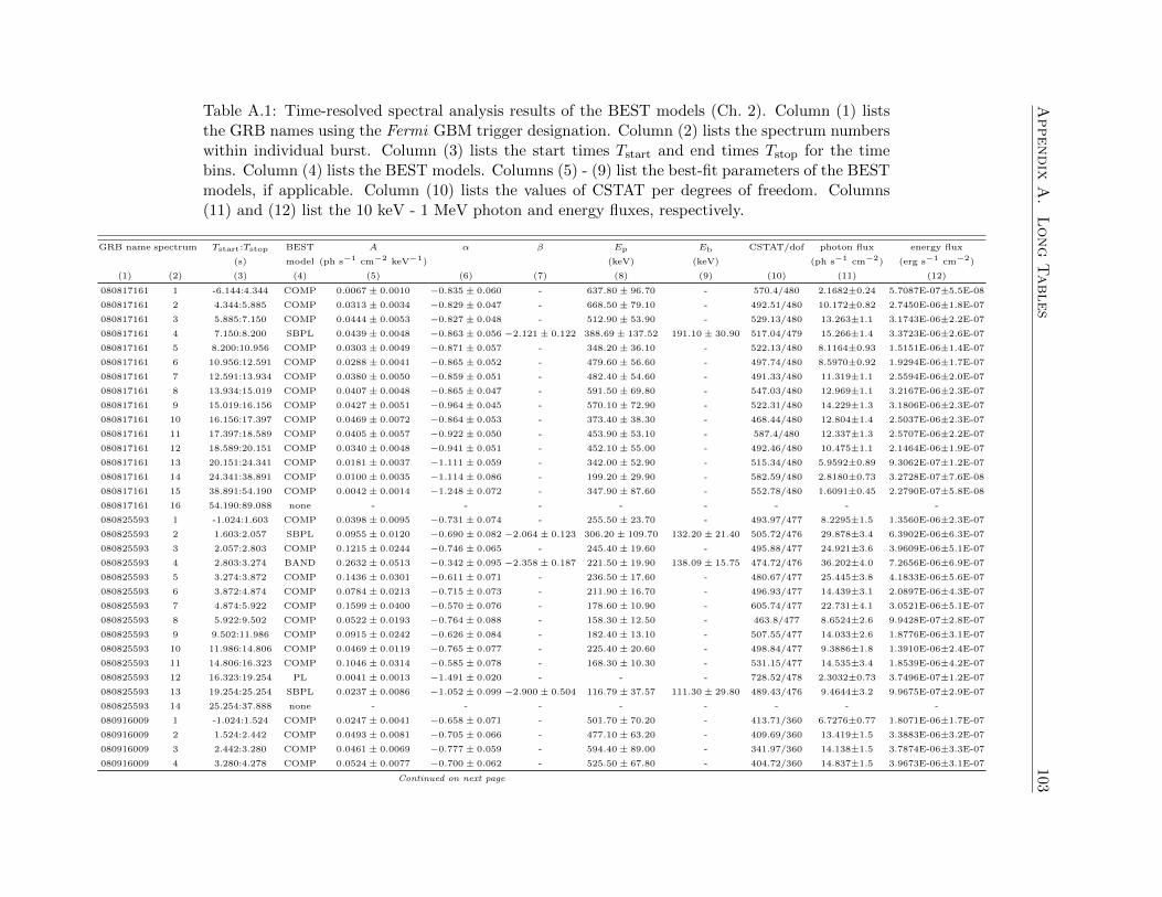
Appendix
A.
Long
Tables
103Table A.1: Time-resolved spectral analysis results of the BEST models (Ch. 2). Column (1) liststhe GRB names using the Fermi GBM trigger designation. Column (2) lists the spectrum numberswithin individual burst. Column (3) lists the start times Tstart and end times Tstop for the timebins. Column (4) lists the BEST models. Columns (5) - (9) list the best-fit parameters of the BESTmodels, if applicable. Column (10) lists the values of CSTAT per degrees of freedom. Columns(11) and (12) list the 10 keV - 1 MeV photon and energy fluxes, respectively.
GRB name spectrum Tstart:Tstop BEST A α β Ep Eb CSTAT/dof photon flux energy flux
(s) model (ph s−1 cm−2 keV−1) (keV) (keV) (ph s−1 cm−2) (erg s−1 cm−2)
(1) (2) (3) (4) (5) (6) (7) (8) (9) (10) (11) (12)
080817161 1 -6.144:4.344 COMP 0.0067± 0.0010 −0.835± 0.060 - 637.80± 96.70 - 570.4/480 2.1682±0.24 5.7087E-07±5.5E-08
080817161 2 4.344:5.885 COMP 0.0313± 0.0034 −0.829± 0.047 - 668.50± 79.10 - 492.51/480 10.172±0.82 2.7450E-06±1.8E-07
080817161 3 5.885:7.150 COMP 0.0444± 0.0053 −0.827± 0.048 - 512.90± 53.90 - 529.13/480 13.263±1.1 3.1743E-06±2.2E-07
080817161 4 7.150:8.200 SBPL 0.0439± 0.0048 −0.863± 0.056 −2.121± 0.122 388.69± 137.52 191.10± 30.90 517.04/479 15.266±1.4 3.3723E-06±2.6E-07
080817161 5 8.200:10.956 COMP 0.0303± 0.0049 −0.871± 0.057 - 348.20± 36.10 - 522.13/480 8.1164±0.93 1.5151E-06±1.4E-07
080817161 6 10.956:12.591 COMP 0.0288± 0.0041 −0.865± 0.052 - 479.60± 56.60 - 497.74/480 8.5970±0.92 1.9294E-06±1.7E-07
080817161 7 12.591:13.934 COMP 0.0380± 0.0050 −0.859± 0.051 - 482.40± 54.60 - 491.33/480 11.319±1.1 2.5594E-06±2.0E-07
080817161 8 13.934:15.019 COMP 0.0407± 0.0048 −0.865± 0.047 - 591.50± 69.80 - 547.03/480 12.969±1.1 3.2167E-06±2.3E-07
080817161 9 15.019:16.156 COMP 0.0427± 0.0051 −0.964± 0.045 - 570.10± 72.90 - 522.31/480 14.229±1.3 3.1806E-06±2.3E-07
080817161 10 16.156:17.397 COMP 0.0469± 0.0072 −0.864± 0.053 - 373.40± 38.30 - 468.44/480 12.804±1.4 2.5037E-06±2.3E-07
080817161 11 17.397:18.589 COMP 0.0405± 0.0057 −0.922± 0.050 - 453.90± 53.10 - 587.4/480 12.337±1.3 2.5707E-06±2.2E-07
080817161 12 18.589:20.151 COMP 0.0340± 0.0048 −0.941± 0.051 - 452.10± 55.00 - 492.46/480 10.475±1.1 2.1464E-06±1.9E-07
080817161 13 20.151:24.341 COMP 0.0181± 0.0037 −1.111± 0.059 - 342.00± 52.90 - 515.34/480 5.9592±0.89 9.3062E-07±1.2E-07
080817161 14 24.341:38.891 COMP 0.0100± 0.0035 −1.114± 0.086 - 199.20± 29.90 - 582.59/480 2.8180±0.73 3.2728E-07±7.6E-08
080817161 15 38.891:54.190 COMP 0.0042± 0.0014 −1.248± 0.072 - 347.90± 87.60 - 552.78/480 1.6091±0.45 2.2790E-07±5.8E-08
080817161 16 54.190:89.088 none - - - - - - - -
080825593 1 -1.024:1.603 COMP 0.0398± 0.0095 −0.731± 0.074 - 255.50± 23.70 - 493.97/477 8.2295±1.5 1.3560E-06±2.3E-07
080825593 2 1.603:2.057 SBPL 0.0955± 0.0120 −0.690± 0.082 −2.064± 0.123 306.20± 109.70 132.20± 21.40 505.72/476 29.878±3.4 6.3902E-06±6.3E-07
080825593 3 2.057:2.803 COMP 0.1215± 0.0244 −0.746± 0.065 - 245.40± 19.60 - 495.88/477 24.921±3.6 3.9609E-06±5.1E-07
080825593 4 2.803:3.274 BAND 0.2632± 0.0513 −0.342± 0.095 −2.358± 0.187 221.50± 19.90 138.09± 15.75 474.72/476 36.202±4.0 7.2656E-06±6.9E-07
080825593 5 3.274:3.872 COMP 0.1436± 0.0301 −0.611± 0.071 - 236.50± 17.60 - 480.67/477 25.445±3.8 4.1833E-06±5.6E-07
080825593 6 3.872:4.874 COMP 0.0784± 0.0213 −0.715± 0.073 - 211.90± 16.70 - 496.93/477 14.439±3.1 2.0897E-06±4.3E-07
080825593 7 4.874:5.922 COMP 0.1599± 0.0400 −0.570± 0.076 - 178.60± 10.90 - 605.74/477 22.731±4.1 3.0521E-06±5.1E-07
080825593 8 5.922:9.502 COMP 0.0522± 0.0193 −0.764± 0.088 - 158.30± 12.50 - 463.8/477 8.6524±2.6 9.9428E-07±2.8E-07
080825593 9 9.502:11.986 COMP 0.0915± 0.0242 −0.626± 0.084 - 182.40± 13.10 - 507.55/477 14.033±2.6 1.8776E-06±3.1E-07
080825593 10 11.986:14.806 COMP 0.0469± 0.0119 −0.765± 0.077 - 225.40± 20.60 - 498.84/477 9.3886±1.8 1.3910E-06±2.4E-07
080825593 11 14.806:16.323 COMP 0.1046± 0.0314 −0.585± 0.078 - 168.30± 10.30 - 531.15/477 14.535±3.4 1.8539E-06±4.2E-07
080825593 12 16.323:19.254 PL 0.0041± 0.0013 −1.491± 0.020 - - - 728.52/478 2.3032±0.73 3.7496E-07±1.2E-07
080825593 13 19.254:25.254 SBPL 0.0237± 0.0086 −1.052± 0.099 −2.900± 0.504 116.79± 37.57 111.30± 29.80 489.43/476 9.4644±3.2 9.9675E-07±2.9E-07
080825593 14 25.254:37.888 none - - - - - - - -
080916009 1 -1.024:1.524 COMP 0.0247± 0.0041 −0.658± 0.071 - 501.70± 70.20 - 413.71/360 6.7276±0.77 1.8071E-06±1.7E-07
080916009 2 1.524:2.442 COMP 0.0493± 0.0081 −0.705± 0.066 - 477.10± 63.20 - 409.69/360 13.419±1.5 3.3883E-06±3.2E-07
080916009 3 2.442:3.280 COMP 0.0461± 0.0069 −0.777± 0.059 - 594.40± 89.00 - 341.97/360 14.138±1.5 3.7874E-06±3.3E-07
080916009 4 3.280:4.278 COMP 0.0524± 0.0077 −0.700± 0.062 - 525.50± 67.80 - 404.72/360 14.837±1.5 3.9673E-06±3.1E-07
Continued on next page
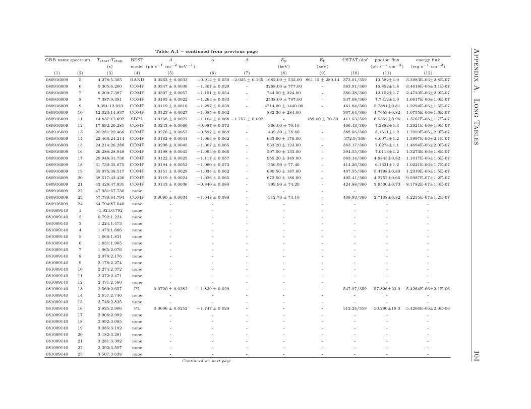
Appendix
A.
Long
Tables
104Table A.1 – continued from previous page
GRB name spectrum Tstart:Tstop BEST A α β Ep Eb CSTAT/dof photon flux energy flux
(s) model (ph s−1 cm−2 keV−1) (keV) (keV) (ph s−1 cm−2) (erg s−1 cm−2)
(1) (2) (3) (4) (5) (6) (7) (8) (9) (10) (11) (12)
080916009 5 4.278:5.305 BAND 0.0263± 0.0033 −0.914± 0.050 −2.025± 0.165 1682.00± 532.00 861.12± 280.14 373.01/359 10.582±1.0 3.3983E-06±2.8E-07
080916009 6 5.305:6.200 COMP 0.0347± 0.0036 −1.307± 0.029 - 3268.00± 777.00 - 383.91/360 16.852±1.8 3.4618E-06±3.1E-07
080916009 7 6.200:7.387 COMP 0.0307± 0.0057 −1.151± 0.054 - 744.50± 224.00 - 380.38/360 12.152±1.7 2.4723E-06±2.9E-07
080916009 8 7.387:9.391 COMP 0.0165± 0.0022 −1.264± 0.033 - 2538.00± 797.00 - 347.08/360 7.7312±1.0 1.6617E-06±1.9E-07
080916009 9 9.391:12.023 COMP 0.0119± 0.0016 −1.297± 0.030 - 4714.00± 1440.00 - 461.84/360 5.7881±0.81 1.2294E-06±1.5E-07
080916009 10 12.023:14.837 COMP 0.0123± 0.0027 −1.085± 0.062 - 832.30± 284.00 - 367.64/360 4.7653±0.82 1.0755E-06±1.6E-07
080916009 11 14.837:17.692 SBPL 0.0158± 0.0027 −1.104± 0.068 −1.757± 0.092 - 189.00± 70.30 411.53/359 6.5352±0.96 1.3767E-06±1.7E-07
080916009 12 17.692:20.281 COMP 0.0243± 0.0060 −0.987± 0.072 - 366.00± 70.10 - 406.43/360 7.2882±1.3 1.2921E-06±1.9E-07
080916009 13 20.281:22.466 COMP 0.0276± 0.0057 −0.897± 0.069 - 439.30± 78.60 - 388.05/360 8.1611±1.2 1.7059E-06±2.0E-07
080916009 14 22.466:24.214 COMP 0.0182± 0.0041 −1.064± 0.062 - 633.60± 176.00 - 372.9/360 6.6074±1.2 1.3997E-06±2.1E-07
080916009 15 24.214:26.288 COMP 0.0208± 0.0045 −1.007± 0.065 - 533.20± 123.00 - 363.17/360 7.0274±1.1 1.4694E-06±2.0E-07
080916009 16 26.288:28.948 COMP 0.0198± 0.0045 −1.093± 0.066 - 507.00± 133.00 - 394.55/360 7.0113±1.2 1.3273E-06±1.8E-07
080916009 17 28.948:31.730 COMP 0.0122± 0.0025 −1.117± 0.057 - 955.20± 349.00 - 363.14/360 4.8843±0.82 1.1017E-06±1.6E-07
080916009 18 31.730:35.075 COMP 0.0194± 0.0053 −1.060± 0.073 - 356.90± 77.40 - 414.26/360 6.1631±1.2 1.0221E-06±1.7E-07
080916009 19 35.075:38.517 COMP 0.0151± 0.0029 −1.034± 0.062 - 690.50± 187.00 - 407.55/360 5.4798±0.80 1.2319E-06±1.5E-07
080916009 20 38.517:43.426 COMP 0.0119± 0.0024 −1.026± 0.065 - 672.50± 186.00 - 405.41/360 4.2752±0.66 9.5987E-07±1.2E-07
080916009 21 43.426:47.931 COMP 0.0143± 0.0036 −0.840± 0.080 - 399.90± 74.20 - 424.88/360 3.9500±0.73 8.1782E-07±1.3E-07
080916009 22 47.931:57.730 none - - - - - - - -
080916009 23 57.730:64.794 COMP 0.0090± 0.0034 −1.048± 0.088 - 312.70± 74.10 - 409.93/360 2.7108±0.82 4.2255E-07±1.2E-07
080916009 24 64.794:87.040 none - - - - - - - -
081009140 1 -1.024:0.792 none - - - - - - - -
081009140 2 0.792:1.224 none - - - - - - - -
081009140 3 1.224:1.473 none - - - - - - - -
081009140 4 1.473:1.666 none - - - - - - - -
081009140 5 1.666:1.831 none - - - - - - - -
081009140 6 1.831:1.965 none - - - - - - - -
081009140 7 1.965:2.076 none - - - - - - - -
081009140 8 2.076:2.176 none - - - - - - - -
081009140 9 2.176:2.274 none - - - - - - - -
081009140 10 2.274:2.372 none - - - - - - - -
081009140 11 2.372:2.471 none - - - - - - - -
081009140 12 2.471:2.560 none - - - - - - - -
081009140 13 2.560:2.657 PL 0.0720± 0.0282 −1.839± 0.029 - - - 547.97/359 57.826±23.0 5.4264E-06±2.1E-06
081009140 14 2.657:2.746 none - - - - - - - -
081009140 15 2.746:2.825 none - - - - - - - -
081009140 16 2.825:2.906 PL 0.0696± 0.0252 −1.747± 0.028 - - - 512.24/359 50.290±19.0 5.4266E-06±2.0E-06
081009140 17 2.906:2.992 none - - - - - - - -
081009140 18 2.992:3.085 none - - - - - - - -
081009140 19 3.085:3.182 none - - - - - - - -
081009140 20 3.182:3.281 none - - - - - - - -
081009140 21 3.281:3.392 none - - - - - - - -
081009140 22 3.392:3.507 none - - - - - - - -
081009140 23 3.507:3.628 none - - - - - - - -
Continued on next page
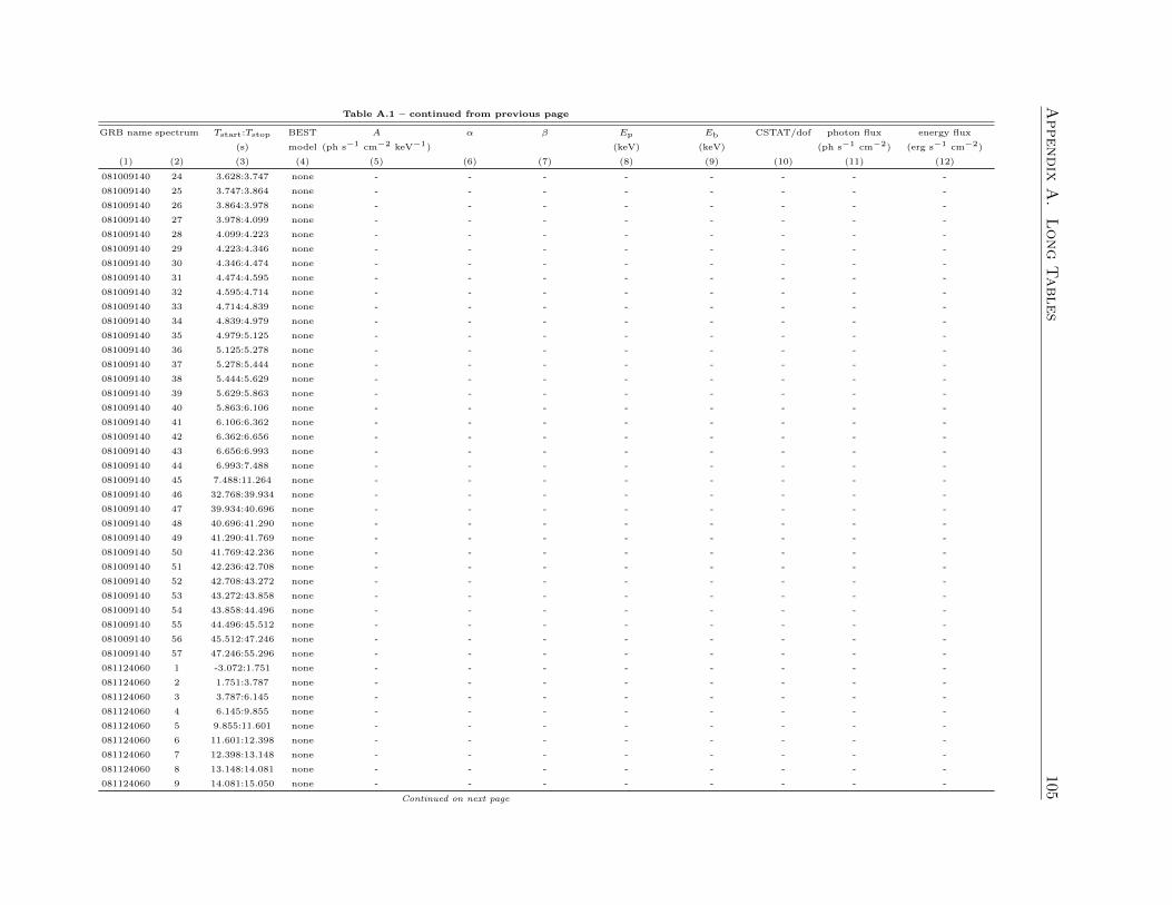
Appendix
A.
Long
Tables
105Table A.1 – continued from previous page
GRB name spectrum Tstart:Tstop BEST A α β Ep Eb CSTAT/dof photon flux energy flux
(s) model (ph s−1 cm−2 keV−1) (keV) (keV) (ph s−1 cm−2) (erg s−1 cm−2)
(1) (2) (3) (4) (5) (6) (7) (8) (9) (10) (11) (12)
081009140 24 3.628:3.747 none - - - - - - - -
081009140 25 3.747:3.864 none - - - - - - - -
081009140 26 3.864:3.978 none - - - - - - - -
081009140 27 3.978:4.099 none - - - - - - - -
081009140 28 4.099:4.223 none - - - - - - - -
081009140 29 4.223:4.346 none - - - - - - - -
081009140 30 4.346:4.474 none - - - - - - - -
081009140 31 4.474:4.595 none - - - - - - - -
081009140 32 4.595:4.714 none - - - - - - - -
081009140 33 4.714:4.839 none - - - - - - - -
081009140 34 4.839:4.979 none - - - - - - - -
081009140 35 4.979:5.125 none - - - - - - - -
081009140 36 5.125:5.278 none - - - - - - - -
081009140 37 5.278:5.444 none - - - - - - - -
081009140 38 5.444:5.629 none - - - - - - - -
081009140 39 5.629:5.863 none - - - - - - - -
081009140 40 5.863:6.106 none - - - - - - - -
081009140 41 6.106:6.362 none - - - - - - - -
081009140 42 6.362:6.656 none - - - - - - - -
081009140 43 6.656:6.993 none - - - - - - - -
081009140 44 6.993:7.488 none - - - - - - - -
081009140 45 7.488:11.264 none - - - - - - - -
081009140 46 32.768:39.934 none - - - - - - - -
081009140 47 39.934:40.696 none - - - - - - - -
081009140 48 40.696:41.290 none - - - - - - - -
081009140 49 41.290:41.769 none - - - - - - - -
081009140 50 41.769:42.236 none - - - - - - - -
081009140 51 42.236:42.708 none - - - - - - - -
081009140 52 42.708:43.272 none - - - - - - - -
081009140 53 43.272:43.858 none - - - - - - - -
081009140 54 43.858:44.496 none - - - - - - - -
081009140 55 44.496:45.512 none - - - - - - - -
081009140 56 45.512:47.246 none - - - - - - - -
081009140 57 47.246:55.296 none - - - - - - - -
081124060 1 -3.072:1.751 none - - - - - - - -
081124060 2 1.751:3.787 none - - - - - - - -
081124060 3 3.787:6.145 none - - - - - - - -
081124060 4 6.145:9.855 none - - - - - - - -
081124060 5 9.855:11.601 none - - - - - - - -
081124060 6 11.601:12.398 none - - - - - - - -
081124060 7 12.398:13.148 none - - - - - - - -
081124060 8 13.148:14.081 none - - - - - - - -
081124060 9 14.081:15.050 none - - - - - - - -
Continued on next page
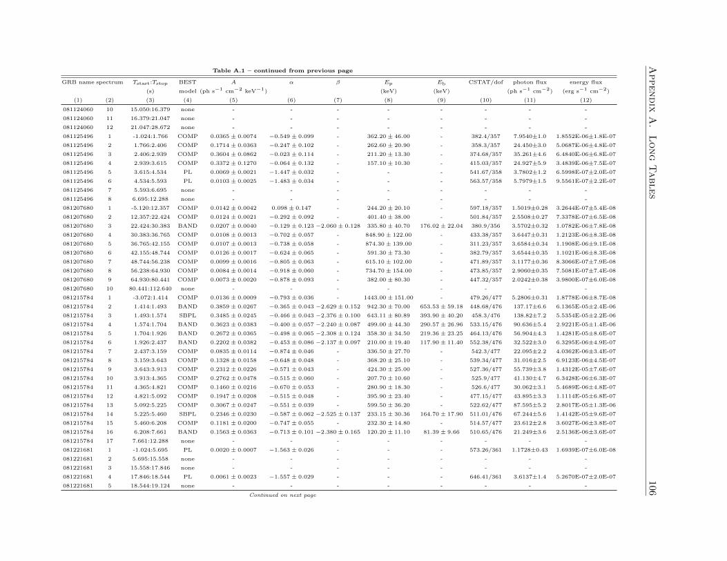
Appendix
A.
Long
Tables
106Table A.1 – continued from previous page
GRB name spectrum Tstart:Tstop BEST A α β Ep Eb CSTAT/dof photon flux energy flux
(s) model (ph s−1 cm−2 keV−1) (keV) (keV) (ph s−1 cm−2) (erg s−1 cm−2)
(1) (2) (3) (4) (5) (6) (7) (8) (9) (10) (11) (12)
081124060 10 15.050:16.379 none - - - - - - - -
081124060 11 16.379:21.047 none - - - - - - - -
081124060 12 21.047:28.672 none - - - - - - - -
081125496 1 -1.024:1.766 COMP 0.0365± 0.0074 −0.549± 0.099 - 362.20± 46.00 - 382.4/357 7.9540±1.0 1.8552E-06±1.8E-07
081125496 2 1.766:2.406 COMP 0.1714± 0.0363 −0.247± 0.102 - 262.60± 20.90 - 358.3/357 24.450±3.0 5.0687E-06±4.8E-07
081125496 3 2.406:2.939 COMP 0.3604± 0.0862 −0.023± 0.114 - 211.20± 13.30 - 374.68/357 35.261±4.6 6.4840E-06±6.8E-07
081125496 4 2.939:3.615 COMP 0.3372± 0.1270 −0.064± 0.132 - 157.10± 10.30 - 415.03/357 24.927±5.9 3.4839E-06±7.5E-07
081125496 5 3.615:4.534 PL 0.0069± 0.0021 −1.447± 0.032 - - - 541.67/358 3.7802±1.2 6.5998E-07±2.0E-07
081125496 6 4.534:5.593 PL 0.0103± 0.0025 −1.483± 0.034 - - - 563.57/358 5.7979±1.5 9.5561E-07±2.2E-07
081125496 7 5.593:6.695 none - - - - - - - -
081125496 8 6.695:12.288 none - - - - - - - -
081207680 1 -5.120:12.357 COMP 0.0142± 0.0042 0.098± 0.147 - 244.20± 20.10 - 597.18/357 1.5019±0.28 3.2644E-07±5.4E-08
081207680 2 12.357:22.424 COMP 0.0124± 0.0021 −0.292± 0.092 - 401.40± 38.00 - 501.84/357 2.5508±0.27 7.3378E-07±6.5E-08
081207680 3 22.424:30.383 BAND 0.0207± 0.0040 −0.129± 0.123 −2.060± 0.128 335.80± 40.70 176.02± 22.04 380.9/356 3.5702±0.32 1.0782E-06±7.8E-08
081207680 4 30.383:36.765 COMP 0.0108± 0.0013 −0.702± 0.057 - 848.90± 122.00 - 433.38/357 3.6447±0.31 1.2123E-06±8.3E-08
081207680 5 36.765:42.155 COMP 0.0107± 0.0013 −0.738± 0.058 - 874.30± 139.00 - 311.23/357 3.6584±0.34 1.1908E-06±9.1E-08
081207680 6 42.155:48.744 COMP 0.0126± 0.0017 −0.624± 0.065 - 591.30± 73.30 - 382.79/357 3.6544±0.35 1.1021E-06±8.3E-08
081207680 7 48.744:56.238 COMP 0.0099± 0.0016 −0.805± 0.063 - 615.10± 102.00 - 471.89/357 3.1177±0.36 8.3066E-07±7.9E-08
081207680 8 56.238:64.930 COMP 0.0084± 0.0014 −0.918± 0.060 - 734.70± 154.00 - 473.85/357 2.9060±0.35 7.5081E-07±7.4E-08
081207680 9 64.930:80.441 COMP 0.0073± 0.0020 −0.878± 0.093 - 382.00± 80.30 - 447.32/357 2.0242±0.38 3.9800E-07±6.0E-08
081207680 10 80.441:112.640 none - - - - - - - -
081215784 1 -3.072:1.414 COMP 0.0136± 0.0009 −0.793± 0.036 - 1443.00± 151.00 - 479.26/477 5.2806±0.31 1.8778E-06±8.7E-08
081215784 2 1.414:1.493 BAND 0.3859± 0.0267 −0.365± 0.043 −2.629± 0.152 942.30± 70.00 653.53± 59.18 448.68/476 137.17±6.6 6.1365E-05±2.4E-06
081215784 3 1.493:1.574 SBPL 0.3485± 0.0245 −0.466± 0.043 −2.376± 0.100 643.11± 80.89 393.90± 40.20 458.3/476 138.82±7.2 5.5354E-05±2.2E-06
081215784 4 1.574:1.704 BAND 0.3623± 0.0383 −0.400± 0.057 −2.240± 0.087 499.00± 44.30 290.57± 26.96 533.15/476 90.636±5.4 2.9221E-05±1.4E-06
081215784 5 1.704:1.926 BAND 0.2672± 0.0365 −0.498± 0.065 −2.308± 0.124 358.30± 34.50 219.36± 23.25 464.13/476 56.904±4.3 1.4281E-05±8.6E-07
081215784 6 1.926:2.437 BAND 0.2202± 0.0382 −0.453± 0.086 −2.137± 0.097 210.00± 19.40 117.90± 11.40 552.38/476 32.522±3.0 6.3295E-06±4.9E-07
081215784 7 2.437:3.159 COMP 0.0835± 0.0114 −0.874± 0.046 - 336.50± 27.70 - 542.3/477 22.095±2.2 4.0362E-06±3.4E-07
081215784 8 3.159:3.643 COMP 0.1328± 0.0158 −0.648± 0.048 - 368.20± 25.10 - 539.34/477 31.016±2.5 6.9123E-06±4.5E-07
081215784 9 3.643:3.913 COMP 0.2312± 0.0226 −0.571± 0.043 - 424.30± 25.00 - 527.36/477 55.739±3.8 1.4312E-05±7.6E-07
081215784 10 3.913:4.365 COMP 0.2762± 0.0478 −0.515± 0.060 - 207.70± 10.60 - 525.9/477 41.130±4.7 6.3428E-06±6.3E-07
081215784 11 4.365:4.821 COMP 0.1460± 0.0216 −0.670± 0.053 - 280.90± 18.30 - 526.6/477 30.062±3.1 5.4689E-06±4.8E-07
081215784 12 4.821:5.092 COMP 0.1947± 0.0208 −0.515± 0.048 - 395.90± 23.40 - 477.15/477 43.895±3.3 1.1114E-05±6.8E-07
081215784 13 5.092:5.225 COMP 0.3067± 0.0247 −0.551± 0.039 - 599.50± 36.20 - 522.62/477 87.595±5.2 2.8017E-05±1.3E-06
081215784 14 5.225:5.460 SBPL 0.2346± 0.0230 −0.587± 0.062 −2.525± 0.137 233.15± 30.36 164.70± 17.90 511.01/476 67.244±5.6 1.4142E-05±9.6E-07
081215784 15 5.460:6.208 COMP 0.1181± 0.0200 −0.747± 0.055 - 232.30± 14.80 - 514.57/477 23.612±2.8 3.6027E-06±3.8E-07
081215784 16 6.208:7.661 BAND 0.1563± 0.0363 −0.713± 0.101 −2.380± 0.165 120.20± 11.10 81.39± 9.66 510.65/476 21.249±3.6 2.5136E-06±3.6E-07
081215784 17 7.661:12.288 none - - - - - - - -
081221681 1 -1.024:5.695 PL 0.0020± 0.0007 −1.563± 0.026 - - - 573.26/361 1.1728±0.43 1.6939E-07±6.0E-08
081221681 2 5.695:15.558 none - - - - - - - -
081221681 3 15.558:17.846 none - - - - - - - -
081221681 4 17.846:18.544 PL 0.0061± 0.0023 −1.557± 0.029 - - - 646.41/361 3.6137±1.4 5.2670E-07±2.0E-07
081221681 5 18.544:19.124 none - - - - - - - -
Continued on next page
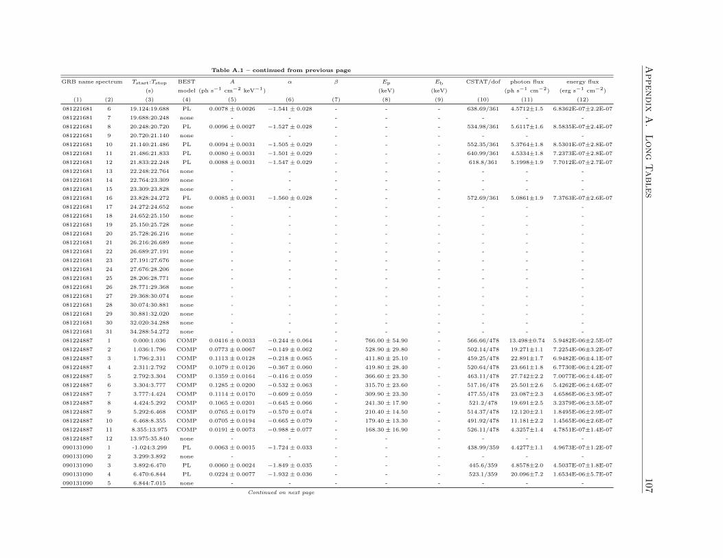
Appendix
A.
Long
Tables
107Table A.1 – continued from previous page
GRB name spectrum Tstart:Tstop BEST A α β Ep Eb CSTAT/dof photon flux energy flux
(s) model (ph s−1 cm−2 keV−1) (keV) (keV) (ph s−1 cm−2) (erg s−1 cm−2)
(1) (2) (3) (4) (5) (6) (7) (8) (9) (10) (11) (12)
081221681 6 19.124:19.688 PL 0.0078± 0.0026 −1.541± 0.028 - - - 638.69/361 4.5712±1.5 6.8362E-07±2.2E-07
081221681 7 19.688:20.248 none - - - - - - - -
081221681 8 20.248:20.720 PL 0.0096± 0.0027 −1.527± 0.028 - - - 534.98/361 5.6117±1.6 8.5835E-07±2.4E-07
081221681 9 20.720:21.140 none - - - - - - - -
081221681 10 21.140:21.486 PL 0.0094± 0.0031 −1.505± 0.029 - - - 552.35/361 5.3764±1.8 8.5301E-07±2.8E-07
081221681 11 21.486:21.833 PL 0.0080± 0.0031 −1.501± 0.029 - - - 640.99/361 4.5334±1.8 7.2373E-07±2.8E-07
081221681 12 21.833:22.248 PL 0.0088± 0.0031 −1.547± 0.029 - - - 618.8/361 5.1998±1.9 7.7012E-07±2.7E-07
081221681 13 22.248:22.764 none - - - - - - - -
081221681 14 22.764:23.309 none - - - - - - - -
081221681 15 23.309:23.828 none - - - - - - - -
081221681 16 23.828:24.272 PL 0.0085± 0.0031 −1.560± 0.028 - - - 572.69/361 5.0861±1.9 7.3763E-07±2.6E-07
081221681 17 24.272:24.652 none - - - - - - - -
081221681 18 24.652:25.150 none - - - - - - - -
081221681 19 25.150:25.728 none - - - - - - - -
081221681 20 25.728:26.216 none - - - - - - - -
081221681 21 26.216:26.689 none - - - - - - - -
081221681 22 26.689:27.191 none - - - - - - - -
081221681 23 27.191:27.676 none - - - - - - - -
081221681 24 27.676:28.206 none - - - - - - - -
081221681 25 28.206:28.771 none - - - - - - - -
081221681 26 28.771:29.368 none - - - - - - - -
081221681 27 29.368:30.074 none - - - - - - - -
081221681 28 30.074:30.881 none - - - - - - - -
081221681 29 30.881:32.020 none - - - - - - - -
081221681 30 32.020:34.288 none - - - - - - - -
081221681 31 34.288:54.272 none - - - - - - - -
081224887 1 0.000:1.036 COMP 0.0416± 0.0033 −0.244± 0.064 - 766.00± 54.90 - 566.66/478 13.498±0.74 5.9482E-06±2.5E-07
081224887 2 1.036:1.796 COMP 0.0773± 0.0067 −0.149± 0.062 - 528.90± 29.80 - 502.14/478 19.271±1.1 7.2254E-06±3.2E-07
081224887 3 1.796:2.311 COMP 0.1113± 0.0128 −0.218± 0.065 - 411.80± 25.10 - 459.25/478 22.891±1.7 6.9482E-06±4.1E-07
081224887 4 2.311:2.792 COMP 0.1079± 0.0126 −0.367± 0.060 - 419.80± 28.40 - 520.64/478 23.661±1.8 6.7730E-06±4.2E-07
081224887 5 2.792:3.304 COMP 0.1359± 0.0164 −0.416± 0.059 - 366.60± 23.30 - 463.11/478 27.742±2.2 7.0077E-06±4.4E-07
081224887 6 3.304:3.777 COMP 0.1285± 0.0200 −0.532± 0.063 - 315.70± 23.60 - 517.16/478 25.501±2.6 5.4262E-06±4.6E-07
081224887 7 3.777:4.424 COMP 0.1114± 0.0170 −0.609± 0.059 - 309.90± 23.30 - 477.55/478 23.087±2.3 4.6586E-06±3.9E-07
081224887 8 4.424:5.292 COMP 0.1065± 0.0201 −0.645± 0.066 - 241.30± 17.90 - 521.2/478 19.691±2.5 3.2379E-06±3.5E-07
081224887 9 5.292:6.468 COMP 0.0765± 0.0179 −0.570± 0.074 - 210.40± 14.50 - 514.37/478 12.120±2.1 1.8495E-06±2.9E-07
081224887 10 6.468:8.355 COMP 0.0705± 0.0194 −0.665± 0.079 - 179.40± 13.30 - 491.92/478 11.181±2.2 1.4565E-06±2.6E-07
081224887 11 8.355:13.975 COMP 0.0191± 0.0073 −0.988± 0.077 - 168.30± 16.90 - 526.11/478 4.3257±1.4 4.7851E-07±1.4E-07
081224887 12 13.975:35.840 none - - - - - - - -
090131090 1 -1.024:3.299 PL 0.0063± 0.0015 −1.724± 0.033 - - - 438.99/359 4.4277±1.1 4.9673E-07±1.2E-07
090131090 2 3.299:3.892 none - - - - - - - -
090131090 3 3.892:6.470 PL 0.0060± 0.0024 −1.849± 0.035 - - - 445.6/359 4.8578±2.0 4.5037E-07±1.8E-07
090131090 4 6.470:6.844 PL 0.0224± 0.0077 −1.932± 0.036 - - - 523.1/359 20.096±7.2 1.6534E-06±5.7E-07
090131090 5 6.844:7.015 none - - - - - - - -
Continued on next page
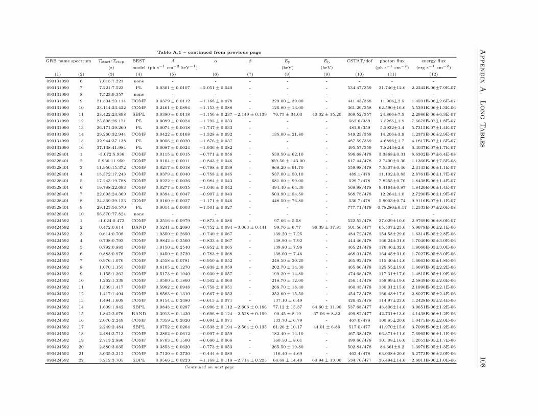
Appendix
A.
Long
Tables
108Table A.1 – continued from previous page
GRB name spectrum Tstart:Tstop BEST A α β Ep Eb CSTAT/dof photon flux energy flux
(s) model (ph s−1 cm−2 keV−1) (keV) (keV) (ph s−1 cm−2) (erg s−1 cm−2)
(1) (2) (3) (4) (5) (6) (7) (8) (9) (10) (11) (12)
090131090 6 7.015:7.221 none - - - - - - - -
090131090 7 7.221:7.523 PL 0.0301± 0.0107 −2.051± 0.040 - - - 534.47/359 31.746±12.0 2.2242E-06±7.9E-07
090131090 8 7.523:9.357 none - - - - - - - -
090131090 9 21.504:23.114 COMP 0.0379± 0.0112 −1.168± 0.078 - 229.00± 39.00 - 441.43/358 11.906±2.5 1.4591E-06±2.6E-07
090131090 10 23.114:23.422 COMP 0.2461± 0.0894 −1.153± 0.088 - 126.80± 13.00 - 361.29/358 62.590±16.0 5.5391E-06±1.3E-06
090131090 11 23.422:23.898 SBPL 0.0380± 0.0118 −1.156± 0.237 −2.149± 0.139 70.75± 34.03 40.02± 15.20 368.52/357 24.866±7.5 2.2986E-06±6.3E-07
090131090 12 23.898:26.171 PL 0.0099± 0.0024 −1.795± 0.033 - - - 562.6/359 7.5285±1.9 7.5678E-07±1.8E-07
090131090 13 26.171:29.260 PL 0.0074± 0.0018 −1.747± 0.033 - - - 481.9/359 5.2932±1.4 5.7315E-07±1.4E-07
090131090 14 29.260:32.944 COMP 0.0422± 0.0168 −1.328± 0.092 - 135.00± 21.80 - 549.23/358 14.206±3.9 1.2373E-06±2.9E-07
090131090 15 32.944:37.138 PL 0.0056± 0.0020 −1.876± 0.037 - - - 487.59/359 4.6896±1.7 4.1817E-07±1.5E-07
090131090 16 37.138:41.984 PL 0.0087± 0.0024 −1.936± 0.082 - - - 495.57/359 7.8243±2.6 6.4037E-07±1.7E-07
090328401 1 -3.072:5.936 COMP 0.0115± 0.0015 −0.771± 0.056 - 530.50± 62.10 - 596.68/478 3.3868±0.31 8.6302E-07±6.4E-08
090328401 2 5.936:11.950 COMP 0.0104± 0.0011 −0.843± 0.046 - 959.50± 143.00 - 617.44/478 3.7400±0.30 1.1366E-06±7.5E-08
090328401 3 11.950:15.372 COMP 0.0217± 0.0018 −0.798± 0.039 - 868.20± 91.70 - 559.98/478 7.5307±0.46 2.3145E-06±1.1E-07
090328401 4 15.372:17.243 COMP 0.0379± 0.0040 −0.758± 0.045 - 537.00± 50.10 - 489.1/478 11.102±0.83 2.8761E-06±1.7E-07
090328401 5 17.243:19.788 COMP 0.0222± 0.0026 −0.984± 0.043 - 681.00± 99.00 - 529.7/478 7.8255±0.70 1.8438E-06±1.4E-07
090328401 6 19.788:22.693 COMP 0.0277± 0.0035 −1.046± 0.042 - 494.40± 64.30 - 568.98/478 9.4164±0.87 1.8420E-06±1.4E-07
090328401 7 22.693:24.369 COMP 0.0394± 0.0047 −0.907± 0.043 - 503.90± 54.50 - 568.75/478 12.264±1.0 2.7290E-06±1.9E-07
090328401 8 24.369:29.123 COMP 0.0160± 0.0027 −1.171± 0.046 - 448.50± 76.80 - 530.7/478 5.9003±0.74 9.9116E-07±1.1E-07
090328401 9 29.123:56.570 PL 0.0014± 0.0003 −1.501± 0.027 - - - 777.71/479 0.78280±0.17 1.2533E-07±2.6E-08
090328401 10 56.570:77.824 none - - - - - - - -
090424592 1 -1.024:0.472 COMP 0.2516± 0.0979 −0.873± 0.086 - 97.66± 5.58 - 522.52/478 37.029±10.0 2.9769E-06±8.0E-07
090424592 2 0.472:0.614 BAND 0.5241± 0.2080 −0.752± 0.094 −3.063± 0.441 99.76± 6.77 96.39± 17.81 501.56/477 65.507±25.0 5.9679E-06±2.1E-06
090424592 3 0.614:0.708 COMP 1.0350± 0.2650 −0.740± 0.067 - 139.20± 7.25 - 484.72/478 154.58±29.0 1.6314E-05±2.8E-06
090424592 4 0.708:0.792 COMP 0.9842± 0.2560 −0.833± 0.067 - 138.90± 7.92 - 444.46/478 166.24±31.0 1.7040E-05±3.0E-06
090424592 5 0.792:0.883 COMP 1.0150± 0.2540 −0.852± 0.065 - 139.80± 7.96 - 465.21/478 176.46±32.0 1.8060E-05±3.0E-06
090424592 6 0.883:0.976 COMP 1.0450± 0.2720 −0.783± 0.068 - 138.00± 7.46 - 468.01/478 164.45±31.0 1.7027E-05±3.0E-06
090424592 7 0.976:1.070 COMP 0.4558± 0.0781 −0.950± 0.052 - 248.50± 20.20 - 465.92/478 115.40±14.0 1.6663E-05±1.8E-06
090424592 8 1.070:1.155 COMP 0.6105± 0.1270 −0.838± 0.059 - 202.70± 14.30 - 465.86/478 125.55±19.0 1.6697E-05±2.2E-06
090424592 9 1.155:1.262 COMP 0.5173± 0.1040 −0.930± 0.057 - 199.20± 14.80 - 474.68/478 117.31±17.0 1.4815E-05±1.9E-06
090424592 10 1.262:1.339 COMP 1.0500± 0.1860 −0.502± 0.060 - 218.70± 12.00 - 456.14/478 159.99±19.0 2.5849E-05±2.6E-06
090424592 11 1.339:1.417 COMP 0.5982± 0.0948 −0.758± 0.051 - 268.70± 18.40 - 460.43/478 130.01±15.0 2.1890E-05±2.1E-06
090424592 12 1.417:1.494 COMP 0.8583± 0.1310 −0.667± 0.052 - 252.60± 15.50 - 454.73/478 166.43±17.0 2.8027E-05±2.4E-06
090424592 13 1.494:1.609 COMP 0.9154± 0.2480 −0.615± 0.071 - 137.10± 6.49 - 426.42/478 114.97±23.0 1.2428E-05±2.4E-06
090424592 14 1.609:1.842 SBPL 0.0843± 0.0287 −0.996± 0.112 −2.606± 0.186 77.12± 15.37 64.60± 11.90 537.68/477 43.806±14.0 3.9651E-06±1.2E-06
090424592 15 1.842:2.076 BAND 0.3913± 0.1420 −0.696± 0.124 −2.528± 0.199 90.45± 8.19 67.06± 8.32 499.82/477 42.731±13.0 4.1438E-06±1.2E-06
090424592 16 2.076:2.249 COMP 0.7359± 0.2020 −0.694± 0.071 - 133.70± 6.79 - 467.0/478 100.85±20.0 1.0475E-05±2.0E-06
090424592 17 2.249:2.484 SBPL 0.0752± 0.0264 −0.538± 0.194 −2.564± 0.135 61.26± 10.17 44.01± 6.86 517.0/477 41.970±15.0 3.7099E-06±1.2E-06
090424592 18 2.484:2.713 COMP 0.2802± 0.0612 −0.997± 0.059 - 182.40± 14.10 - 467.38/478 66.371±11.0 7.6965E-06±1.1E-06
090424592 19 2.713:2.880 COMP 0.6703± 0.1500 −0.680± 0.066 - 160.50± 8.61 - 499.66/478 101.08±16.0 1.2053E-05±1.7E-06
090424592 20 2.880:3.035 COMP 0.3853± 0.0620 −0.773± 0.053 - 265.50± 19.80 - 502.84/478 84.361±9.2 1.3979E-05±1.3E-06
090424592 21 3.035:3.212 COMP 0.7130± 0.2730 −0.444± 0.080 - 116.40± 4.69 - 462.4/478 63.008±20.0 6.2773E-06±2.0E-06
090424592 22 3.212:3.705 SBPL 0.0566± 0.0223 −1.168± 0.118 −2.714± 0.225 64.68± 14.40 60.94± 13.00 534.76/477 36.494±14.0 2.8011E-06±1.0E-06
Continued on next page
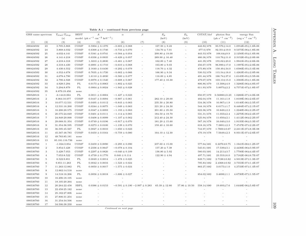
Appendix
A.
Long
Tables
109Table A.1 – continued from previous page
GRB name spectrum Tstart:Tstop BEST A α β Ep Eb CSTAT/dof photon flux energy flux
(s) model (ph s−1 cm−2 keV−1) (keV) (keV) (ph s−1 cm−2) (erg s−1 cm−2)
(1) (2) (3) (4) (5) (6) (7) (8) (9) (10) (11) (12)
090424592 23 3.705:3.868 COMP 0.5904± 0.1370 −0.603± 0.068 - 167.50± 9.22 - 442.82/478 83.576±14.0 1.0554E-05±1.6E-06
090424592 24 3.868:4.032 COMP 0.6368± 0.1740 −0.733± 0.070 - 134.70± 7.01 - 477.0/478 92.351±19.0 9.5375E-06±1.8E-06
090424592 25 4.032:4.141 COMP 0.5341± 0.0741 −0.584± 0.054 - 299.80± 19.00 - 443.53/478 106.64±9.9 2.1256E-05±1.6E-06
090424592 26 4.141:4.218 COMP 0.6336± 0.0935 −0.429± 0.057 - 289.90± 16.40 - 480.36/478 110.76±11.0 2.3152E-05±2.0E-06
090424592 27 4.218:4.318 COMP 1.3210± 0.2830 −0.461± 0.067 - 162.00± 7.40 - 441.39/478 155.02±23.0 1.9941E-05±2.6E-06
090424592 28 4.318:4.430 COMP 0.6891± 0.1710 −0.610± 0.068 - 163.80± 9.03 - 456.67/478 96.890±17.0 1.1997E-05±2.0E-06
090424592 29 4.430:4.552 COMP 2.1640± 0.6430 −0.292± 0.079 - 118.70± 4.32 - 475.89/478 158.49±34.0 1.6586E-05±3.4E-06
090424592 30 4.552:4.678 COMP 0.7635± 0.1720 −0.662± 0.066 - 166.90± 9.34 - 530.52/478 115.54±18.0 1.4263E-05±2.0E-06
090424592 31 4.678:4.790 COMP 1.6110± 0.4930 −0.560± 0.077 - 116.00± 4.85 - 491.44/478 166.74±37.0 1.6145E-05±3.5E-06
090424592 32 4.790:4.928 COMP 0.6978± 0.1540 −0.608± 0.067 - 177.40± 10.30 - 479.07/478 103.13±15.0 1.3583E-05±1.8E-06
090424592 33 4.928:5.294 PL 0.0173± 0.0063 −1.802± 0.025 - - - 806.86/479 13.308±4.9 1.3206E-06±4.8E-07
090424592 34 5.294:8.879 PL 0.0064± 0.0024 −1.943± 0.028 - - - 611.93/479 5.8975±2.2 4.7571E-07±1.8E-07
090424592 35 8.879:19.456 none - - - - - - - -
090528516 1 -6.144:8.064 PL 0.0011± 0.0004 −1.427± 0.023 - - - 850.97/479 0.56880±0.23 1.0266E-07±4.0E-08
090528516 2 8.064:10.077 COMP 0.0447± 0.0094 −0.887± 0.061 - 282.10± 29.00 - 492.04/478 11.161±1.8 1.8109E-06±2.6E-07
090528516 3 10.077:12.531 COMP 0.0495± 0.0112 −0.843± 0.063 - 235.30± 20.80 - 534.36/478 10.967±1.9 1.6140E-06±2.5E-07
090528516 4 12.531:16.200 COMP 0.0244± 0.0075 −1.049± 0.063 - 221.20± 24.30 - 544.18/478 6.6171±1.7 8.4484E-07±2.1E-07
090528516 5 16.200:20.575 COMP 0.0347± 0.0093 −1.193± 0.063 - 201.80± 25.50 - 622.36/478 10.849±2.2 1.2246E-06±2.2E-07
090528516 6 20.575:24.849 COMP 0.0401± 0.0111 −1.114± 0.065 - 184.50± 19.70 - 531.31/478 11.033±2.4 1.2270E-06±2.4E-07
090528516 7 24.849:29.068 COMP 0.0408± 0.0099 −1.107± 0.062 - 212.40± 24.30 - 525.94/478 11.650±2.1 1.4112E-06±2.2E-07
090528516 8 29.068:31.354 COMP 0.0749± 0.0196 −0.917± 0.070 - 181.20± 15.60 - 567.18/478 16.040±3.0 1.9135E-06±3.3E-07
090528516 9 31.354:36.595 COMP 0.0273± 0.0100 −1.139± 0.070 - 159.40± 16.60 - 618.16/478 7.3891±2.3 7.4747E-07±2.2E-07
090528516 10 36.595:45.567 PL 0.0027± 0.0010 −1.650± 0.023 - - - 744.97/479 1.7800±0.67 2.2411E-07±8.3E-08
090528516 11 45.567:48.783 COMP 0.0450± 0.0164 −0.759± 0.080 - 164.10± 12.30 - 470.19/478 7.5649±2.3 8.9311E-07±2.6E-07
090528516 12 48.783:85.181 none - - - - - - - -
090528516 13 85.181:116.736 none - - - - - - - -
090530760 1 -1.024:3.854 COMP 0.0459± 0.0090 −0.295± 0.090 - 237.60± 15.00 - 577.64/481 6.2276±0.75 1.1641E-06±1.2E-07
090530760 2 3.854:5.428 COMP 0.2336± 0.0647 −0.078± 0.104 - 157.20± 7.38 - 545.61/481 17.539±3.1 2.4436E-06±3.9E-07
090530760 3 5.428:7.053 COMP 0.2297± 0.0820 −0.040± 0.109 - 136.80± 5.92 - 580.03/481 14.211±3.7 1.7700E-06±4.4E-07
090530760 4 7.053:8.522 COMP 0.4739± 0.1770 0.040± 0.114 - 122.90± 4.94 - 497.71/481 23.553±6.0 2.7182E-06±6.7E-07
090530760 5 8.522:9.851 PL 0.0049± 0.0014 −1.478± 0.025 - - - 849.71/482 2.7188±0.82 4.5013E-07±1.3E-07
090530760 6 9.851:11.263 PL 0.0042± 0.0016 −1.523± 0.024 - - - 795.83/482 2.4368±0.92 3.7555E-07±1.4E-07
090530760 7 11.263:12.882 PL 0.0050± 0.0017 −1.575± 0.024 - - - 883.27/482 3.0175±1.0 4.2733E-07±1.4E-07
090530760 8 12.882:14.518 none - - - - - - - -
090530760 9 14.518:16.206 PL 0.0056± 0.0018 −1.606± 0.027 - - - 854.02/482 3.4698±1.1 4.6730E-07±1.5E-07
090530760 10 16.206:18.105 none - - - - - - - -
090530760 11 18.105:20.264 none - - - - - - - -
090530760 12 20.264:22.458 SBPL 0.0386± 0.0153 −0.591± 0.190 −2.997± 0.283 65.39± 12.80 57.86± 10.50 558.14/480 19.693±7.6 1.6448E-06±5.8E-07
090530760 13 22.458:25.182 none - - - - - - - -
090530760 14 25.182:27.806 none - - - - - - - -
090530760 15 27.806:31.254 none - - - - - - - -
090530760 16 31.254:34.506 none - - - - - - - -
090530760 17 34.506:38.230 none - - - - - - - -
Continued on next page
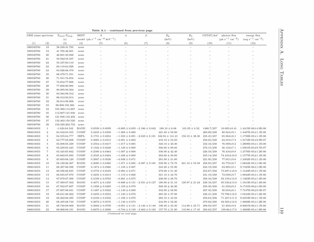
Appendix
A.
Long
Tables
110Table A.1 – continued from previous page
GRB name spectrum Tstart:Tstop BEST A α β Ep Eb CSTAT/dof photon flux energy flux
(s) model (ph s−1 cm−2 keV−1) (keV) (keV) (ph s−1 cm−2) (erg s−1 cm−2)
(1) (2) (3) (4) (5) (6) (7) (8) (9) (10) (11) (12)
090530760 18 38.230:41.795 none - - - - - - - -
090530760 19 41.795:46.001 none - - - - - - - -
090530760 20 46.001:50.922 none - - - - - - - -
090530760 21 50.922:55.337 none - - - - - - - -
090530760 22 55.337:60.110 none - - - - - - - -
090530760 23 60.110:64.928 none - - - - - - - -
090530760 24 64.928:68.479 none - - - - - - - -
090530760 25 68.479:71.551 none - - - - - - - -
090530760 26 71.551:74.654 none - - - - - - - -
090530760 27 74.654:77.868 none - - - - - - - -
090530760 28 77.868:80.995 none - - - - - - - -
090530760 29 80.995:84.364 none - - - - - - - -
090530760 30 84.364:88.312 none - - - - - - - -
090530760 31 88.312:92.914 none - - - - - - - -
090530760 32 92.914:98.808 none - - - - - - - -
090530760 33 98.808:105.360 none - - - - - - - -
090530760 34 105.360:112.867 none - - - - - - - -
090530760 35 112.867:121.936 none - - - - - - - -
090530760 36 121.936:132.402 none - - - - - - - -
090530760 37 132.402:150.320 none - - - - - - - -
090530760 38 150.320:202.752 none - - - - - - - -
090618353 1 -1.024:64.342 BAND 0.0539± 0.0039 −0.805± 0.033 −2.186± 0.042 168.10± 6.88 101.05± 4.52 1488.7/237 10.005±0.41 1.4415E-06±4.9E-08
090618353 2 64.342:64.555 COMP 0.2433± 0.0358 −1.068± 0.060 - 421.40± 56.60 - 260.66/238 80.944±9.1 1.4487E-05±1.1E-06
090618353 3 64.555:64.777 SBPL 0.1731± 0.0254 −1.033± 0.091 −2.049± 0.101 342.94± 141.21 150.10± 38.30 235.45/237 65.364±8.1 1.1758E-05±1.1E-06
090618353 4 64.777:65.008 COMP 0.2065± 0.0315 −0.991± 0.063 - 416.10± 53.50 - 250.05/238 64.310±7.3 1.2174E-05±9.9E-07
090618353 5 65.008:65.239 COMP 0.2554± 0.0417 −1.017± 0.065 - 340.10± 40.30 - 222.16/238 76.599±9.2 1.2808E-05±1.1E-06
090618353 6 65.239:65.445 COMP 0.1542± 0.0248 −1.129± 0.060 - 506.60± 90.60 - 272.15/238 56.134±7.1 1.0301E-05±9.7E-07
090618353 7 65.445:65.662 COMP 0.2580± 0.0464 −1.007± 0.068 - 336.00± 42.40 - 226.33/238 76.416±9.9 1.2776E-05±1.2E-06
090618353 8 65.662:65.893 COMP 0.2545± 0.0494 −1.028± 0.069 - 302.60± 39.00 - 233.14/238 74.410±10.0 1.1577E-05±1.1E-06
090618353 9 65.893:66.120 COMP 0.2907± 0.0526 −0.938± 0.071 - 291.60± 31.60 - 221.95/238 77.051±9.6 1.2402E-05±1.1E-06
090618353 10 66.120:66.367 BAND 0.2080± 0.0460 −1.071± 0.085 −2.387± 0.165 339.90± 73.70 241.16± 55.58 256.05/237 65.770±8.7 1.0824E-05±1.0E-06
090618353 11 66.367:66.598 COMP 0.1874± 0.0366 −1.150± 0.067 - 343.20± 55.90 - 223.19/238 63.905±9.1 9.7425E-06±1.0E-06
090618353 12 66.598:66.835 COMP 0.2776± 0.0523 −0.984± 0.071 - 278.90± 31.40 - 253.67/238 75.697±10.0 1.1540E-05±1.1E-06
090618353 13 66.835:67.070 COMP 0.2235± 0.0414 −1.110± 0.066 - 321.10± 44.70 - 231.19/238 72.039±9.7 1.0944E-05±1.1E-06
090618353 14 67.070:67.309 COMP 0.3199± 0.0703 −0.981± 0.075 - 238.00± 26.70 - 256.16/238 82.159±12.0 1.1383E-05±1.3E-06
090618353 15 67.309:67.562 BAND 0.4071± 0.1250 −0.888± 0.131 −2.331± 0.127 180.80± 31.10 120.97± 21.24 229.18/237 85.545±13.0 1.1813E-05±1.4E-06
090618353 16 67.562:67.807 COMP 0.1938± 0.0409 −1.103± 0.070 - 308.30± 46.20 - 256.39/238 61.350±9.3 9.1741E-06±1.0E-06
090618353 17 67.807:68.041 COMP 0.1487± 0.0322 −1.149± 0.069 - 342.00± 58.90 - 287.45/238 50.634±8.1 7.7107E-06±9.5E-07
090618353 18 68.041:68.262 COMP 0.2450± 0.0552 −1.120± 0.072 - 265.30± 37.80 - 236.41/238 75.798±12.0 1.0344E-05±1.2E-06
090618353 19 68.262:68.495 COMP 0.2102± 0.0452 −1.188± 0.070 - 283.10± 43.50 - 258.64/238 71.257±11.0 9.6353E-06±1.1E-06
090618353 20 68.495:68.740 COMP 0.2670± 0.0576 −1.140± 0.073 - 244.90± 32.20 - 279.82/238 82.565±12.0 1.0666E-05±1.2E-06
090618353 21 68.740:68.968 BAND 0.2602± 0.0799 −0.951± 0.131 −2.146± 0.140 196.40± 43.30 114.88± 25.71 268.93/237 61.403±9.6 8.9081E-06±1.1E-06
090618353 22 68.968:69.191 BAND 0.6670± 0.2090 −0.744± 0.139 −2.462± 0.183 157.70± 21.90 110.88± 17.45 256.63/237 109.86±17.0 1.4669E-05±1.8E-06
Continued on next page
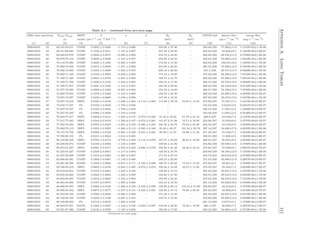
Appendix
A.
Long
Tables
111Table A.1 – continued from previous page
GRB name spectrum Tstart:Tstop BEST A α β Ep Eb CSTAT/dof photon flux energy flux
(s) model (ph s−1 cm−2 keV−1) (keV) (keV) (ph s−1 cm−2) (erg s−1 cm−2)
(1) (2) (3) (4) (5) (6) (7) (8) (9) (10) (11) (12)
090618353 23 69.191:69.411 COMP 0.2255± 0.0429 −1.173± 0.066 - 316.20± 47.40 - 256.46/238 77.209±11.0 1.1131E-05±1.1E-06
090618353 24 69.411:69.649 COMP 0.1536± 0.0311 −1.155± 0.067 - 351.30± 59.00 - 253.25/238 52.934±8.0 8.1283E-06±9.4E-07
090618353 25 69.649:69.879 COMP 0.2648± 0.0675 −0.996± 0.084 - 214.70± 24.90 - 228.48/238 66.535±11.0 8.5768E-06±1.2E-06
090618353 26 69.879:70.116 COMP 0.2626± 0.0598 −1.131± 0.075 - 233.80± 30.30 - 232.81/238 79.260±13.0 1.0033E-05±1.2E-06
090618353 27 70.116:70.389 COMP 0.4628± 0.1290 −0.966± 0.088 - 172.90± 17.30 - 262.04/238 102.83±18.0 1.1695E-05±1.7E-06
090618353 28 70.389:70.636 COMP 0.2575± 0.0659 −1.071± 0.082 - 213.00± 26.50 - 265.52/238 70.368±12.0 8.7084E-06±1.2E-06
090618353 29 70.636:70.909 COMP 0.2438± 0.0580 −1.084± 0.076 - 230.10± 29.20 - 231.1/238 69.417±11.0 8.9292E-06±1.1E-06
090618353 30 70.909:71.160 COMP 0.3129± 0.0992 −0.952± 0.093 - 174.10± 19.00 - 247.62/238 68.530±14.0 7.8724E-06±1.4E-06
090618353 31 71.160:71.430 COMP 0.2645± 0.0734 −1.047± 0.086 - 188.70± 21.70 - 269.36/238 67.268±13.0 7.8251E-06±1.2E-06
090618353 32 71.430:71.706 COMP 0.3940± 0.1210 −1.043± 0.090 - 160.10± 17.30 - 260.37/238 93.735±19.0 9.8682E-06±1.6E-06
090618353 33 71.706:71.977 COMP 0.3201± 0.1030 −1.110± 0.091 - 165.30± 20.30 - 286.42/238 84.164±18.0 8.8132E-06±1.5E-06
090618353 34 71.977:72.290 COMP 0.3209± 0.1020 −0.991± 0.094 - 164.70± 18.00 - 266.57/238 72.160±15.0 7.8790E-06±1.3E-06
090618353 35 72.290:72.655 COMP 0.1558± 0.0496 −1.163± 0.089 - 182.50± 25.30 - 260.32/238 45.389±10.0 4.9256E-06±9.3E-07
090618353 36 72.655:73.097 COMP 0.2439± 0.0869 −1.048± 0.098 - 147.20± 16.50 - 287.95/238 56.472±13.0 5.6373E-06±1.1E-06
090618353 37 73.097:73.618 SBPL 0.0596± 0.0136 −1.088± 0.204 −2.112± 0.064 114.08± 39.18 53.85± 14.50 274.69/237 31.367±7.0 3.4441E-06±6.8E-07
090618353 38 73.618:74.257 PL 0.0120± 0.0042 −1.720± 0.036 - - - 324.03/239 8.3443±3.0 9.4231E-07±3.3E-07
090618353 39 74.257:75.257 PL 0.0162± 0.0034 −1.769± 0.034 - - - 348.54/239 11.901±2.8 1.2469E-06±2.6E-07
090618353 40 75.257:76.463 PL 0.0088± 0.0030 −1.724± 0.034 - - - 334.58/239 6.1955±2.2 6.9548E-07±2.3E-07
090618353 41 76.463:77.317 SBPL 0.0402± 0.0141 −1.223± 0.175 −2.379± 0.223 81.42± 32.64 61.70± 21.10 260.8/237 23.540±7.8 2.1247E-06±6.3E-07
090618353 42 77.317:77.945 SBPL 0.0544± 0.0118 −1.236± 0.187 −2.072± 0.061 121.47± 51.98 53.71± 16.90 254.06/237 31.032±6.6 3.2797E-06±6.1E-07
090618353 43 77.945:78.482 SBPL 0.0707± 0.0219 −1.091± 0.150 −2.486± 0.261 100.30± 33.76 79.03± 23.20 262.33/237 33.139±9.5 3.3892E-06±8.4E-07
090618353 44 78.482:79.115 SBPL 0.1053± 0.0355 −1.294± 0.113 −2.920± 0.443 93.49± 30.57 101.40± 30.70 297.14/237 54.690±17.0 4.6635E-06±1.2E-06
090618353 45 79.115:79.706 SBPL 0.0560± 0.0122 −0.981± 0.349 −2.044± 0.061 90.98± 41.55 34.68± 11.50 271.49/237 34.133±7.4 3.4944E-06±6.6E-07
090618353 46 79.706:80.155 PL 0.0191± 0.0044 −1.614± 0.035 - - - 339.81/239 11.928±2.9 1.5945E-06±3.6E-07
090618353 47 80.155:80.538 SBPL 0.0755± 0.0174 −0.779± 0.259 −2.118± 0.070 107.57± 35.03 46.65± 10.90 268.21/237 36.585±8.2 4.2529E-06±8.4E-07
090618353 48 80.538:80.874 COMP 0.2180± 0.0693 −1.149± 0.089 - 169.60± 21.90 - 254.86/238 60.928±13.0 6.3788E-06±1.2E-06
090618353 49 80.874:81.227 SBPL 0.0681± 0.0171 −0.973± 0.252 −2.096± 0.070 102.95± 41.48 44.56± 12.10 273.86/237 37.049±9.1 4.0001E-06±8.7E-07
090618353 50 81.227:81.627 COMP 0.2328± 0.0815 −1.117± 0.094 - 146.30± 16.70 - 239.98/238 59.185±14.0 5.7550E-06±1.2E-06
090618353 51 81.627:82.008 COMP 0.1212± 0.0420 −1.285± 0.087 - 171.50± 27.10 - 234.73/238 40.813±10.0 4.0728E-06±9.0E-07
090618353 52 82.008:82.381 COMP 0.1806± 0.0581 −1.148± 0.090 - 169.10± 22.00 - 271.54/238 50.368±11.0 5.2667E-06±9.9E-07
090618353 53 82.381:82.788 BAND 0.1692± 0.0662 −0.871± 0.171 −2.100± 0.068 126.70± 24.30 73.16± 13.23 275.82/237 29.921±6.4 3.7820E-06±7.2E-07
090618353 54 82.788:83.219 SBPL 0.0659± 0.0150 −0.824± 0.285 −2.072± 0.072 109.46± 44.62 43.57± 11.60 270.59/237 33.433±7.4 3.8549E-06±7.5E-07
090618353 55 83.219:83.655 COMP 0.2152± 0.0854 −1.022± 0.105 - 138.30± 15.10 - 291.02/238 46.851±13.0 4.5374E-06±1.1E-06
090618353 56 83.655:84.062 COMP 0.2023± 0.0664 −1.202± 0.088 - 162.60± 21.90 - 250.61/238 59.910±13.0 6.0044E-06±1.1E-06
090618353 57 84.062:84.365 COMP 0.2216± 0.0605 −1.124± 0.083 - 193.00± 24.30 - 275.03/238 62.554±12.0 7.1274E-06±1.1E-06
090618353 58 84.365:84.696 COMP 0.3167± 0.0975 −1.085± 0.088 - 162.10± 18.50 - 281.14/238 80.049±16.0 8.3598E-06±1.4E-06
090618353 59 84.696:84.995 SBPL 0.0960± 0.0188 −1.268± 0.103 −2.162± 0.099 192.89± 69.13 110.10± 31.80 228.66/237 44.414±8.4 5.5703E-06±8.9E-07
090618353 60 84.995:85.352 SBPL 0.0872± 0.0177 −1.237± 0.141 −2.162± 0.061 130.82± 37.14 76.26± 20.40 255.93/237 43.899±8.8 4.9122E-06±8.7E-07
090618353 61 85.352:85.746 COMP 0.2790± 0.0958 −0.960± 0.099 - 151.50± 15.50 - 263.56/238 58.067±13.0 6.0743E-06±1.2E-06
090618353 62 85.746:86.166 COMP 0.3232± 0.1180 −0.887± 0.104 - 140.70± 13.30 - 278.96/238 58.939±14.0 6.0098E-06±1.3E-06
090618353 63 86.166:86.604 PL 0.0143± 0.0045 −1.662± 0.035 - - - 291.12/239 9.3577±3.1 1.1592E-06±3.6E-07
090618353 64 86.604:87.021 BAND 0.1464± 0.0557 −1.104± 0.166 −2.030± 0.087 133.60± 36.20 72.56± 18.58 286.1/237 36.680±7.3 4.3931E-06±7.6E-07
090618353 65 87.021:87.386 COMP 0.2149± 0.0709 −1.102± 0.093 - 156.40± 17.80 - 260.12/238 54.808±12.0 5.5716E-06±1.1E-06
Continued on next page
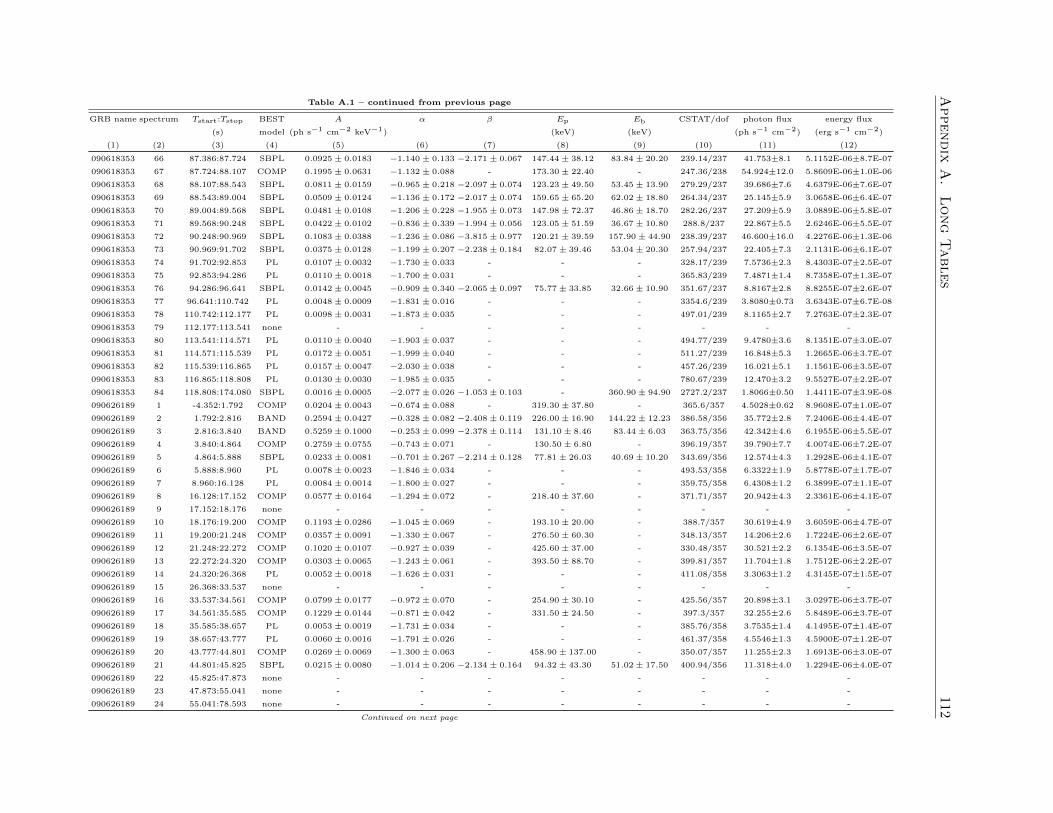
Appendix
A.
Long
Tables
112Table A.1 – continued from previous page
GRB name spectrum Tstart:Tstop BEST A α β Ep Eb CSTAT/dof photon flux energy flux
(s) model (ph s−1 cm−2 keV−1) (keV) (keV) (ph s−1 cm−2) (erg s−1 cm−2)
(1) (2) (3) (4) (5) (6) (7) (8) (9) (10) (11) (12)
090618353 66 87.386:87.724 SBPL 0.0925± 0.0183 −1.140± 0.133 −2.171± 0.067 147.44± 38.12 83.84± 20.20 239.14/237 41.753±8.1 5.1152E-06±8.7E-07
090618353 67 87.724:88.107 COMP 0.1995± 0.0631 −1.132± 0.088 - 173.30± 22.40 - 247.36/238 54.924±12.0 5.8609E-06±1.0E-06
090618353 68 88.107:88.543 SBPL 0.0811± 0.0159 −0.965± 0.218 −2.097± 0.074 123.23± 49.50 53.45± 13.90 279.29/237 39.686±7.6 4.6379E-06±7.6E-07
090618353 69 88.543:89.004 SBPL 0.0509± 0.0124 −1.136± 0.172 −2.017± 0.074 159.65± 65.20 62.02± 18.80 264.34/237 25.145±5.9 3.0658E-06±6.4E-07
090618353 70 89.004:89.568 SBPL 0.0481± 0.0108 −1.206± 0.228 −1.955± 0.073 147.98± 72.37 46.86± 18.70 282.26/237 27.209±5.9 3.0889E-06±5.8E-07
090618353 71 89.568:90.248 SBPL 0.0422± 0.0102 −0.836± 0.339 −1.994± 0.056 123.05± 51.59 36.67± 10.80 288.8/237 22.867±5.5 2.6246E-06±5.5E-07
090618353 72 90.248:90.969 SBPL 0.1083± 0.0388 −1.236± 0.086 −3.815± 0.977 120.21± 39.59 157.90± 44.90 238.39/237 46.600±16.0 4.2276E-06±1.3E-06
090618353 73 90.969:91.702 SBPL 0.0375± 0.0128 −1.199± 0.207 −2.238± 0.184 82.07± 39.46 53.04± 20.30 257.94/237 22.405±7.3 2.1131E-06±6.1E-07
090618353 74 91.702:92.853 PL 0.0107± 0.0032 −1.730± 0.033 - - - 328.17/239 7.5736±2.3 8.4303E-07±2.5E-07
090618353 75 92.853:94.286 PL 0.0110± 0.0018 −1.700± 0.031 - - - 365.83/239 7.4871±1.4 8.7358E-07±1.3E-07
090618353 76 94.286:96.641 SBPL 0.0142± 0.0045 −0.909± 0.340 −2.065± 0.097 75.77± 33.85 32.66± 10.90 351.67/237 8.8167±2.8 8.8255E-07±2.6E-07
090618353 77 96.641:110.742 PL 0.0048± 0.0009 −1.831± 0.016 - - - 3354.6/239 3.8080±0.73 3.6343E-07±6.7E-08
090618353 78 110.742:112.177 PL 0.0098± 0.0031 −1.873± 0.035 - - - 497.01/239 8.1165±2.7 7.2763E-07±2.3E-07
090618353 79 112.177:113.541 none - - - - - - - -
090618353 80 113.541:114.571 PL 0.0110± 0.0040 −1.903± 0.037 - - - 494.77/239 9.4780±3.6 8.1351E-07±3.0E-07
090618353 81 114.571:115.539 PL 0.0172± 0.0051 −1.999± 0.040 - - - 511.27/239 16.848±5.3 1.2665E-06±3.7E-07
090618353 82 115.539:116.865 PL 0.0157± 0.0047 −2.030± 0.038 - - - 457.26/239 16.021±5.1 1.1561E-06±3.5E-07
090618353 83 116.865:118.808 PL 0.0130± 0.0030 −1.985± 0.035 - - - 780.67/239 12.470±3.2 9.5527E-07±2.2E-07
090618353 84 118.808:174.080 SBPL 0.0016± 0.0005 −2.077± 0.026 −1.053± 0.103 - 360.90± 94.90 2727.2/237 1.8066±0.50 1.4411E-07±3.9E-08
090626189 1 -4.352:1.792 COMP 0.0204± 0.0043 −0.674± 0.088 - 319.30± 37.80 - 365.6/357 4.5028±0.62 8.9608E-07±1.0E-07
090626189 2 1.792:2.816 BAND 0.2594± 0.0427 −0.328± 0.082 −2.408± 0.119 226.00± 16.90 144.22± 12.23 386.58/356 35.772±2.8 7.2406E-06±4.4E-07
090626189 3 2.816:3.840 BAND 0.5259± 0.1000 −0.253± 0.099 −2.378± 0.114 131.10± 8.46 83.44± 6.03 363.75/356 42.342±4.6 6.1955E-06±5.5E-07
090626189 4 3.840:4.864 COMP 0.2759± 0.0755 −0.743± 0.071 - 130.50± 6.80 - 396.19/357 39.790±7.7 4.0074E-06±7.2E-07
090626189 5 4.864:5.888 SBPL 0.0233± 0.0081 −0.701± 0.267 −2.214± 0.128 77.81± 26.03 40.69± 10.20 343.69/356 12.574±4.3 1.2928E-06±4.1E-07
090626189 6 5.888:8.960 PL 0.0078± 0.0023 −1.846± 0.034 - - - 493.53/358 6.3322±1.9 5.8778E-07±1.7E-07
090626189 7 8.960:16.128 PL 0.0084± 0.0014 −1.800± 0.027 - - - 359.75/358 6.4308±1.2 6.3899E-07±1.1E-07
090626189 8 16.128:17.152 COMP 0.0577± 0.0164 −1.294± 0.072 - 218.40± 37.60 - 371.71/357 20.942±4.3 2.3361E-06±4.1E-07
090626189 9 17.152:18.176 none - - - - - - - -
090626189 10 18.176:19.200 COMP 0.1193± 0.0286 −1.045± 0.069 - 193.10± 20.00 - 388.7/357 30.619±4.9 3.6059E-06±4.7E-07
090626189 11 19.200:21.248 COMP 0.0357± 0.0091 −1.330± 0.067 - 276.50± 60.30 - 348.13/357 14.206±2.6 1.7224E-06±2.6E-07
090626189 12 21.248:22.272 COMP 0.1020± 0.0107 −0.927± 0.039 - 425.60± 37.00 - 330.48/357 30.521±2.2 6.1354E-06±3.5E-07
090626189 13 22.272:24.320 COMP 0.0303± 0.0065 −1.243± 0.061 - 393.50± 88.70 - 399.81/357 11.704±1.8 1.7512E-06±2.2E-07
090626189 14 24.320:26.368 PL 0.0052± 0.0018 −1.626± 0.031 - - - 411.08/358 3.3063±1.2 4.3145E-07±1.5E-07
090626189 15 26.368:33.537 none - - - - - - - -
090626189 16 33.537:34.561 COMP 0.0799± 0.0177 −0.972± 0.070 - 254.90± 30.10 - 425.56/357 20.898±3.1 3.0297E-06±3.7E-07
090626189 17 34.561:35.585 COMP 0.1229± 0.0144 −0.871± 0.042 - 331.50± 24.50 - 397.3/357 32.255±2.6 5.8489E-06±3.7E-07
090626189 18 35.585:38.657 PL 0.0053± 0.0019 −1.731± 0.034 - - - 385.76/358 3.7535±1.4 4.1495E-07±1.4E-07
090626189 19 38.657:43.777 PL 0.0060± 0.0016 −1.791± 0.026 - - - 461.37/358 4.5546±1.3 4.5900E-07±1.2E-07
090626189 20 43.777:44.801 COMP 0.0269± 0.0069 −1.300± 0.063 - 458.90± 137.00 - 350.07/357 11.255±2.3 1.6913E-06±3.0E-07
090626189 21 44.801:45.825 SBPL 0.0215± 0.0080 −1.014± 0.206 −2.134± 0.164 94.32± 43.30 51.02± 17.50 400.94/356 11.318±4.0 1.2294E-06±4.0E-07
090626189 22 45.825:47.873 none - - - - - - - -
090626189 23 47.873:55.041 none - - - - - - - -
090626189 24 55.041:78.593 none - - - - - - - -
Continued on next page
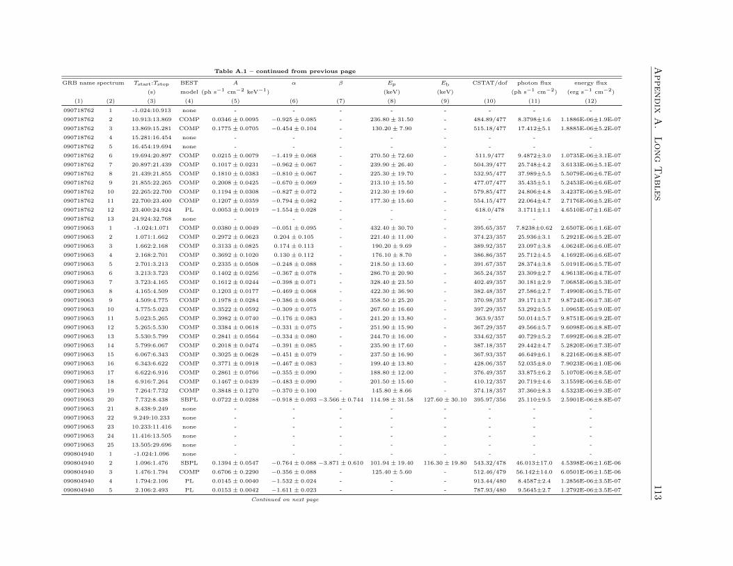
Appendix
A.
Long
Tables
113Table A.1 – continued from previous page
GRB name spectrum Tstart:Tstop BEST A α β Ep Eb CSTAT/dof photon flux energy flux
(s) model (ph s−1 cm−2 keV−1) (keV) (keV) (ph s−1 cm−2) (erg s−1 cm−2)
(1) (2) (3) (4) (5) (6) (7) (8) (9) (10) (11) (12)
090718762 1 -1.024:10.913 none - - - - - - - -
090718762 2 10.913:13.869 COMP 0.0346± 0.0095 −0.925± 0.085 - 236.80± 31.50 - 484.89/477 8.3798±1.6 1.1886E-06±1.9E-07
090718762 3 13.869:15.281 COMP 0.1775± 0.0705 −0.454± 0.104 - 130.20± 7.90 - 515.18/477 17.412±5.1 1.8885E-06±5.2E-07
090718762 4 15.281:16.454 none - - - - - - - -
090718762 5 16.454:19.694 none - - - - - - - -
090718762 6 19.694:20.897 COMP 0.0215± 0.0079 −1.419± 0.068 - 270.50± 72.60 - 511.9/477 9.4872±3.0 1.0735E-06±3.1E-07
090718762 7 20.897:21.439 COMP 0.1017± 0.0231 −0.962± 0.067 - 239.90± 26.40 - 504.39/477 25.748±4.2 3.6133E-06±5.1E-07
090718762 8 21.439:21.855 COMP 0.1810± 0.0383 −0.810± 0.067 - 225.30± 19.70 - 532.95/477 37.989±5.5 5.5079E-06±6.7E-07
090718762 9 21.855:22.265 COMP 0.2008± 0.0425 −0.670± 0.069 - 213.10± 15.50 - 477.07/477 35.435±5.1 5.2453E-06±6.6E-07
090718762 10 22.265:22.700 COMP 0.1194± 0.0308 −0.827± 0.072 - 212.30± 19.60 - 579.85/477 24.806±4.8 3.4237E-06±5.9E-07
090718762 11 22.700:23.400 COMP 0.1207± 0.0359 −0.794± 0.082 - 177.30± 15.60 - 554.15/477 22.064±4.7 2.7176E-06±5.2E-07
090718762 12 23.400:24.924 PL 0.0053± 0.0019 −1.554± 0.028 - - - 618.0/478 3.1711±1.1 4.6510E-07±1.6E-07
090718762 13 24.924:32.768 none - - - - - - - -
090719063 1 -1.024:1.071 COMP 0.0380± 0.0049 −0.051± 0.095 - 432.40± 30.70 - 395.65/357 7.8238±0.62 2.6507E-06±1.6E-07
090719063 2 1.071:1.662 COMP 0.2972± 0.0623 0.204± 0.105 - 221.40± 11.00 - 374.23/357 25.936±3.1 5.2921E-06±5.2E-07
090719063 3 1.662:2.168 COMP 0.3133± 0.0825 0.174± 0.113 - 190.20± 9.69 - 389.92/357 23.097±3.8 4.0624E-06±6.0E-07
090719063 4 2.168:2.701 COMP 0.3692± 0.1020 0.130± 0.112 - 176.10± 8.70 - 386.86/357 25.712±4.5 4.1692E-06±6.6E-07
090719063 5 2.701:3.213 COMP 0.2335± 0.0508 −0.248± 0.088 - 218.50± 13.60 - 391.67/357 28.374±3.8 5.0191E-06±5.7E-07
090719063 6 3.213:3.723 COMP 0.1402± 0.0256 −0.367± 0.078 - 286.70± 20.90 - 365.24/357 23.309±2.7 4.9613E-06±4.7E-07
090719063 7 3.723:4.165 COMP 0.1612± 0.0244 −0.398± 0.071 - 328.40± 23.50 - 402.49/357 30.181±2.9 7.0685E-06±5.3E-07
090719063 8 4.165:4.509 COMP 0.1203± 0.0177 −0.469± 0.068 - 422.30± 36.90 - 382.48/357 27.586±2.7 7.4990E-06±5.7E-07
090719063 9 4.509:4.775 COMP 0.1978± 0.0284 −0.386± 0.068 - 358.50± 25.20 - 370.98/357 39.171±3.7 9.8724E-06±7.3E-07
090719063 10 4.775:5.023 COMP 0.3522± 0.0592 −0.309± 0.075 - 267.60± 16.60 - 397.29/357 53.292±5.5 1.0965E-05±9.0E-07
090719063 11 5.023:5.265 COMP 0.3982± 0.0740 −0.176± 0.083 - 241.20± 13.80 - 363.9/357 50.014±5.7 9.8751E-06±9.2E-07
090719063 12 5.265:5.530 COMP 0.3384± 0.0618 −0.331± 0.075 - 251.90± 15.90 - 367.29/357 49.566±5.7 9.6098E-06±8.8E-07
090719063 13 5.530:5.799 COMP 0.2841± 0.0564 −0.334± 0.080 - 244.70± 16.00 - 334.62/357 40.729±5.2 7.6992E-06±8.2E-07
090719063 14 5.799:6.067 COMP 0.2018± 0.0474 −0.391± 0.085 - 235.90± 17.60 - 387.18/357 29.442±4.7 5.2820E-06±7.3E-07
090719063 15 6.067:6.343 COMP 0.3025± 0.0628 −0.451± 0.079 - 237.50± 16.90 - 367.93/357 46.649±6.1 8.2216E-06±8.8E-07
090719063 16 6.343:6.622 COMP 0.3771± 0.0918 −0.467± 0.083 - 199.40± 13.80 - 428.06/357 52.035±8.0 7.9023E-06±1.0E-06
090719063 17 6.622:6.916 COMP 0.2861± 0.0766 −0.355± 0.090 - 188.80± 12.00 - 376.49/357 33.875±6.2 5.1070E-06±8.5E-07
090719063 18 6.916:7.264 COMP 0.1467± 0.0439 −0.483± 0.090 - 201.50± 15.60 - 410.12/357 20.719±4.6 3.1559E-06±6.5E-07
090719063 19 7.264:7.732 COMP 0.3848± 0.1270 −0.370± 0.100 - 145.80± 8.66 - 374.18/357 37.360±8.3 4.5323E-06±9.3E-07
090719063 20 7.732:8.438 SBPL 0.0722± 0.0288 −0.918± 0.093 −3.566± 0.744 114.98± 31.58 127.60± 30.10 395.97/356 25.110±9.5 2.5901E-06±8.8E-07
090719063 21 8.438:9.249 none - - - - - - - -
090719063 22 9.249:10.233 none - - - - - - - -
090719063 23 10.233:11.416 none - - - - - - - -
090719063 24 11.416:13.505 none - - - - - - - -
090719063 25 13.505:29.696 none - - - - - - - -
090804940 1 -1.024:1.096 none - - - - - - - -
090804940 2 1.096:1.476 SBPL 0.1394± 0.0547 −0.764± 0.088 −3.871± 0.610 101.94± 19.40 116.30± 19.80 543.32/478 46.013±17.0 4.5398E-06±1.6E-06
090804940 3 1.476:1.794 COMP 0.6706± 0.2290 −0.356± 0.088 - 125.40± 5.60 - 512.46/479 56.142±14.0 6.0501E-06±1.5E-06
090804940 4 1.794:2.106 PL 0.0145± 0.0040 −1.532± 0.024 - - - 913.44/480 8.4587±2.4 1.2856E-06±3.5E-07
090804940 5 2.106:2.493 PL 0.0153± 0.0042 −1.611± 0.023 - - - 787.93/480 9.5645±2.7 1.2792E-06±3.5E-07
Continued on next page
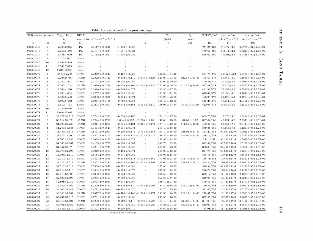
Appendix
A.
Long
Tables
114Table A.1 – continued from previous page
GRB name spectrum Tstart:Tstop BEST A α β Ep Eb CSTAT/dof photon flux energy flux
(s) model (ph s−1 cm−2 keV−1) (keV) (keV) (ph s−1 cm−2) (erg s−1 cm−2)
(1) (2) (3) (4) (5) (6) (7) (8) (9) (10) (11) (12)
090804940 6 2.493:2.965 PL 0.0117± 0.0036 −1.589± 0.023 - - - 751.95/480 7.1972±2.3 9.9707E-07±3.0E-07
090804940 7 2.965:3.488 PL 0.0104± 0.0034 −1.591± 0.024 - - - 760.61/480 6.3911±2.1 8.8227E-07±2.8E-07
090804940 8 3.488:4.070 PL 0.0112± 0.0041 −1.696± 0.026 - - - 836.02/480 7.6591±2.8 8.9418E-07±3.2E-07
090804940 9 4.070:4.651 none - - - - - - - -
090804940 10 4.651:5.569 none - - - - - - - -
090804940 11 5.569:7.879 none - - - - - - - -
090804940 12 7.879:11.264 none - - - - - - - -
090809978 1 -2.048:2.205 COMP 0.0240± 0.0043 −0.477± 0.086 - 397.60± 44.40 - 561.74/479 5.3192±0.62 1.3793E-06±1.4E-07
090809978 2 2.205:2.786 BAND 0.2072± 0.0442 −0.242± 0.112 −2.138± 0.128 229.00± 23.80 127.58± 13.81 475.67/478 27.466±3.0 6.1689E-06±5.6E-07
090809978 3 2.786:3.267 COMP 0.1164± 0.0204 −0.626± 0.065 - 331.00± 30.20 - 490.58/479 25.327±3.1 5.3084E-06±5.5E-07
090809978 4 3.267:3.764 BAND 0.1970± 0.0439 −0.538± 0.104 −2.114± 0.149 205.90± 26.00 114.51± 16.04 517.48/478 31.119±4.1 5.7865E-06±6.5E-07
090809978 5 3.764:4.286 COMP 0.1810± 0.0404 −0.664± 0.072 - 221.30± 17.50 - 491.37/479 32.453±4.9 4.9559E-06±6.5E-07
090809978 6 4.286:4.884 COMP 0.2257± 0.0659 −0.609± 0.083 - 168.90± 11.90 - 513.34/479 32.350±6.6 4.1018E-06±7.7E-07
090809978 7 4.884:5.590 COMP 0.1003± 0.0306 −0.964± 0.074 - 189.90± 20.00 - 496.93/479 23.198±5.4 2.7984E-06±5.9E-07
090809978 8 5.590:6.552 COMP 0.1081± 0.0408 −0.769± 0.085 - 155.40± 12.60 - 515.28/479 17.851±5.3 2.0196E-06±5.7E-07
090809978 9 6.552:7.733 SBPL 0.0205± 0.0077 −0.944± 0.161 −2.113± 0.140 108.05± 43.84 54.67± 14.50 512.04/478 9.8556±3.6 1.1562E-06±4.0E-07
090809978 10 7.733:9.646 none - - - - - - - -
090809978 11 9.646:27.648 none - - - - - - - -
090820027 1 28.672:30.712 COMP 0.0742± 0.0263 −0.723± 0.100 - 174.10± 17.60 - 369.73/359 12.370±3.0 1.5426E-06±3.3E-07
090820027 2 30.712:31.028 BAND 0.6224± 0.1790 0.004± 0.157 −2.275± 0.150 147.50± 13.60 87.60± 8.62 397.84/358 42.721±6.5 7.5879E-06±9.5E-07
090820027 3 31.028:31.263 BAND 0.5011± 0.1260 −0.195± 0.124 −2.371± 0.177 179.10± 16.50 111.51± 12.03 402.66/358 50.554±7.3 9.3144E-06±1.1E-06
090820027 4 31.263:31.434 COMP 0.3474± 0.0624 −0.505± 0.071 - 263.10± 18.40 - 389.38/359 60.155±7.4 1.1251E-05±1.2E-06
090820027 5 31.434:31.575 BAND 0.8441± 0.2000 −0.200± 0.113 −2.533± 0.188 193.40± 16.50 128.94± 13.43 313.29/358 90.913±12.0 1.7025E-05±1.8E-06
090820027 6 31.575:31.700 BAND 0.9801± 0.2370 −0.132± 0.113 −2.704± 0.216 198.50± 16.10 139.91± 14.49 356.14/358 101.19±13.0 1.9234E-05±2.0E-06
090820027 7 31.700:31.833 COMP 0.6098± 0.1170 −0.340± 0.074 - 238.90± 14.40 - 354.1/359 86.246±11.0 1.5929E-05±1.7E-06
090820027 8 31.833:31.957 COMP 0.4103± 0.0765 −0.608± 0.067 - 281.70± 22.50 - 322.91/359 80.515±10.0 1.5129E-05±1.6E-06
090820027 9 31.957:32.078 COMP 0.4201± 0.0735 −0.600± 0.065 - 296.90± 23.30 - 366.08/359 84.427±10.0 1.6566E-05±1.6E-06
090820027 10 32.078:32.195 COMP 0.5319± 0.0961 −0.454± 0.071 - 268.00± 18.30 - 371.75/359 89.626±11.0 1.7391E-05±1.7E-06
090820027 11 32.195:32.310 COMP 0.5584± 0.0995 −0.541± 0.066 - 265.90± 18.70 - 365.75/359 100.25±12.0 1.8596E-05±1.8E-06
090820027 12 32.310:32.417 SBPL 0.4421± 0.0616 −0.254± 0.118 −2.502± 0.162 173.04± 28.10 111.70± 14.30 336.78/358 109.56±14.0 2.1262E-05±2.2E-06
090820027 13 32.417:32.513 BAND 0.9351± 0.2180 −0.233± 0.109 −2.532± 0.191 208.60± 18.50 138.86± 15.15 315.23/358 110.89±14.0 2.1627E-05±2.2E-06
090820027 14 32.513:32.614 COMP 0.5500± 0.0958 −0.512± 0.066 - 275.80± 19.00 - 340.94/359 98.817±12.0 1.9112E-05±1.9E-06
090820027 15 32.614:32.710 COMP 0.8534± 0.1750 −0.364± 0.075 - 231.90± 14.60 - 296.74/359 120.14±16.0 2.1452E-05±2.3E-06
090820027 16 32.710:32.806 COMP 0.6300± 0.1090 −0.523± 0.067 - 267.50± 18.20 - 390.12/359 111.92±13.0 2.1028E-05±2.0E-06
090820027 17 32.806:32.898 COMP 0.8355± 0.1450 −0.512± 0.066 - 262.60± 17.10 - 319.05/359 145.29±17.0 2.7043E-05±2.4E-06
090820027 18 32.898:32.982 COMP 0.5663± 0.1040 −0.545± 0.067 - 288.50± 21.80 - 379.56/359 107.29±13.0 2.1171E-05±2.1E-06
090820027 19 32.982:33.066 BAND 1.3290± 0.3230 −0.239± 0.110 −2.648± 0.203 189.80± 16.00 133.27± 13.92 310.34/358 145.13±19.0 2.5902E-05±2.8E-06
090820027 20 33.066:33.148 COMP 0.8781± 0.1610 −0.492± 0.070 - 243.70± 15.80 - 312.45/359 142.84±17.0 2.5267E-05±2.5E-06
090820027 21 33.148:33.231 BAND 0.9817± 0.2330 −0.410± 0.106 −2.428± 0.171 198.50± 20.20 129.23± 14.80 279.57/358 131.61±17.0 2.3531E-05±2.5E-06
090820027 22 33.231:33.315 COMP 0.7701± 0.1440 −0.502± 0.068 - 246.50± 16.00 - 359.45/359 127.35±16.0 2.2635E-05±2.4E-06
090820027 23 33.315:33.401 BAND 1.3960± 0.3390 −0.212± 0.110 −2.718± 0.220 185.40± 14.70 133.37± 14.09 361.08/358 145.16±19.0 2.5422E-05±2.8E-06
090820027 24 33.401:33.486 SBPL 0.5732± 0.0870 −0.501± 0.089 −2.835± 0.227 164.34± 24.50 133.50± 17.40 342.99/358 151.15±21.0 2.5684E-05±2.9E-06
090820027 25 33.486:33.570 COMP 0.7321± 0.1460 −0.509± 0.072 - 234.60± 15.80 - 354.98/359 117.80±16.0 2.0068E-05±2.3E-06
Continued on next page
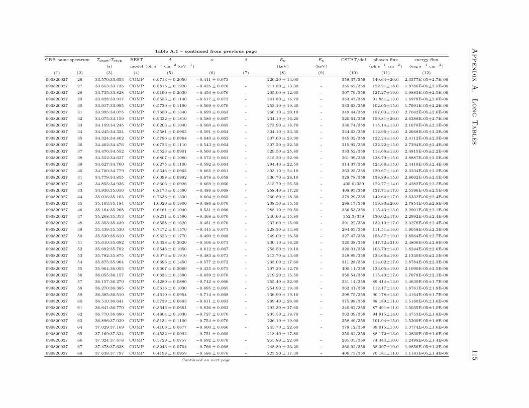
Appendix
A.
Long
Tables
115Table A.1 – continued from previous page
GRB name spectrum Tstart:Tstop BEST A α β Ep Eb CSTAT/dof photon flux energy flux
(s) model (ph s−1 cm−2 keV−1) (keV) (keV) (ph s−1 cm−2) (erg s−1 cm−2)
(1) (2) (3) (4) (5) (6) (7) (8) (9) (10) (11) (12)
090820027 26 33.570:33.653 COMP 0.9713± 0.2050 −0.441± 0.073 - 220.20± 14.00 - 358.37/359 140.64±20.0 2.3377E-05±2.7E-06
090820027 27 33.653:33.735 COMP 0.8816± 0.1920 −0.425± 0.076 - 211.80± 13.30 - 355.62/359 122.21±18.0 1.9786E-05±2.5E-06
090820027 28 33.735:33.828 COMP 0.9190± 0.2030 −0.450± 0.076 - 205.00± 12.60 - 307.79/359 127.27±19.0 1.9883E-05±2.5E-06
090820027 29 33.828:33.917 COMP 0.5553± 0.1140 −0.517± 0.072 - 241.80± 16.70 - 353.47/359 91.851±13.0 1.5978E-05±2.0E-06
090820027 30 33.917:33.995 COMP 0.5730± 0.1190 −0.569± 0.070 - 253.10± 19.40 - 333.63/359 102.05±15.0 1.7991E-05±2.2E-06
090820027 31 33.995:34.075 COMP 0.7650± 0.1340 −0.699± 0.063 - 266.10± 20.10 - 349.44/359 157.03±19.0 2.7042E-05±2.6E-06
090820027 32 34.075:34.159 COMP 0.9332± 0.1810 −0.580± 0.067 - 234.10± 16.20 - 320.64/359 159.81±20.0 2.6388E-05±2.7E-06
090820027 33 34.159:34.245 COMP 0.6203± 0.1040 −0.560± 0.065 - 273.90± 18.70 - 330.74/359 115.14±13.0 2.1670E-05±2.1E-06
090820027 34 34.245:34.324 COMP 0.5581± 0.0965 −0.591± 0.064 - 304.10± 23.30 - 334.63/359 112.96±14.0 2.2668E-05±2.2E-06
090820027 35 34.324:34.402 COMP 0.5786± 0.0964 −0.640± 0.062 - 307.60± 23.90 - 345.02/359 122.24±14.0 2.4112E-05±2.3E-06
090820027 36 34.402:34.476 COMP 0.6723± 0.1110 −0.543± 0.064 - 307.20± 22.50 - 315.92/359 132.22±15.0 2.7394E-05±2.4E-06
090820027 37 34.476:34.552 COMP 0.5523± 0.0901 −0.560± 0.063 - 329.50± 25.80 - 333.52/359 114.68±13.0 2.4815E-05±2.2E-06
090820027 38 34.552:34.627 COMP 0.6807± 0.1080 −0.572± 0.061 - 315.20± 22.90 - 361.99/359 138.79±15.0 2.8887E-05±2.5E-06
090820027 39 34.627:34.700 COMP 0.6275± 0.1100 −0.592± 0.064 - 294.40± 22.50 - 314.37/359 124.68±15.0 2.4419E-05±2.4E-06
090820027 40 34.700:34.779 COMP 0.5646± 0.0965 −0.665± 0.061 - 303.10± 24.10 - 363.25/359 120.67±14.0 2.3234E-05±2.2E-06
090820027 41 34.779:34.855 COMP 0.6098± 0.0982 −0.678± 0.059 - 336.70± 28.10 - 328.78/359 138.89±15.0 2.8602E-05±2.5E-06
090820027 42 34.855:34.936 COMP 0.5606± 0.0926 −0.669± 0.060 - 315.70± 25.50 - 405.0/359 122.77±14.0 2.4282E-05±2.2E-06
090820027 43 34.936:35.016 COMP 0.8173± 0.1490 −0.486± 0.068 - 258.40± 17.20 - 408.95/359 137.71±17.0 2.5596E-05±2.5E-06
090820027 44 35.016:35.103 COMP 0.7636± 0.1330 −0.604± 0.065 - 260.80± 18.30 - 379.29/359 142.64±17.0 2.5332E-05±2.4E-06
090820027 45 35.103:35.184 COMP 1.0020± 0.1900 −0.486± 0.070 - 238.50± 15.50 - 298.17/359 159.83±20.0 2.7854E-05±2.8E-06
090820027 46 35.184:35.268 COMP 0.6161± 0.1040 −0.531± 0.066 - 288.10± 20.50 - 336.53/359 115.43±13.0 2.2901E-05±2.1E-06
090820027 47 35.268:35.353 COMP 0.8231± 0.1590 −0.468± 0.070 - 240.60± 15.80 - 352.3/359 130.02±17.0 2.2992E-05±2.4E-06
090820027 48 35.353:35.439 COMP 0.8558± 0.1620 −0.451± 0.070 - 237.60± 15.00 - 391.22/359 132.10±17.0 2.3278E-05±2.4E-06
090820027 49 35.439:35.530 COMP 0.7472± 0.1570 −0.445± 0.073 - 228.30± 14.80 - 294.65/359 111.51±16.0 1.9058E-05±2.3E-06
090820027 50 35.530:35.610 COMP 0.9623± 0.1770 −0.490± 0.068 - 249.00± 16.50 - 327.47/359 158.57±19.0 2.8564E-05±2.7E-06
090820027 51 35.610:35.692 COMP 0.9328± 0.2020 −0.506± 0.073 - 230.10± 16.20 - 320.08/359 147.72±21.0 2.4806E-05±2.8E-06
090820027 52 35.692:35.782 COMP 0.5546± 0.1050 −0.612± 0.067 - 258.50± 19.10 - 320.01/359 103.79±14.0 1.8244E-05±2.0E-06
090820027 53 35.782:35.875 COMP 0.9073± 0.1910 −0.483± 0.073 - 213.70± 13.60 - 348.89/359 133.66±19.0 2.1340E-05±2.5E-06
090820027 54 35.875:35.964 COMP 0.6696± 0.1450 −0.577± 0.072 - 233.00± 17.60 - 311.28/359 114.02±17.0 1.8784E-05±2.3E-06
090820027 55 35.964:36.055 COMP 0.9667± 0.2060 −0.435± 0.075 - 207.30± 12.70 - 400.11/359 133.05±19.0 2.1090E-05±2.5E-06
090820027 56 36.055:36.157 COMP 0.6634± 0.1390 −0.639± 0.070 - 219.20± 15.50 - 350.54/359 115.43±17.0 1.7678E-05±2.1E-06
090820027 57 36.157:36.270 COMP 0.4280± 0.0880 −0.742± 0.066 - 255.40± 22.00 - 331.14/359 89.414±13.0 1.4630E-05±1.7E-06
090820027 58 36.270:36.385 COMP 0.5616± 0.1030 −0.695± 0.065 - 254.90± 19.40 - 362.41/359 112.17±14.0 1.8761E-05±1.9E-06
090820027 59 36.385:36.510 COMP 0.4610± 0.0954 −0.714± 0.068 - 236.90± 19.10 - 398.75/359 90.178±13.0 1.4164E-05±1.7E-06
090820027 60 36.510:36.641 COMP 0.3739± 0.0683 −0.811± 0.063 - 289.40± 26.90 - 375.98/359 88.189±11.0 1.5180E-05±1.6E-06
090820027 61 36.641:36.770 COMP 0.3646± 0.0661 −0.826± 0.062 - 292.30± 27.60 - 340.62/359 87.491±11.0 1.5035E-05±1.5E-06
090820027 62 36.770:36.896 COMP 0.4804± 0.1030 −0.727± 0.070 - 235.50± 19.70 - 362.09/359 94.915±14.0 1.4753E-05±1.8E-06
090820027 63 36.896:37.029 COMP 0.5134± 0.1100 −0.754± 0.070 - 226.10± 19.00 - 358.49/359 101.94±15.0 1.5200E-05±1.8E-06
090820027 64 37.029:37.169 COMP 0.4108± 0.0877 −0.800± 0.066 - 245.70± 22.60 - 378.12/359 89.015±13.0 1.3774E-05±1.6E-06
090820027 65 37.169:37.324 COMP 0.4532± 0.0992 −0.751± 0.069 - 218.40± 17.80 - 350.62/359 88.172±13.0 1.2830E-05±1.6E-06
090820027 66 37.324:37.478 COMP 0.3729± 0.0757 −0.692± 0.070 - 255.80± 22.00 - 285.05/359 74.444±10.0 1.2498E-05±1.4E-06
090820027 67 37.478:37.638 COMP 0.3243± 0.0704 −0.766± 0.068 - 248.80± 23.20 - 360.92/359 68.397±10.0 1.0856E-05±1.3E-06
090820027 68 37.638:37.797 COMP 0.4198± 0.0959 −0.586± 0.076 - 223.20± 17.30 - 406.73/359 70.181±11.0 1.1141E-05±1.4E-06
Continued on next page
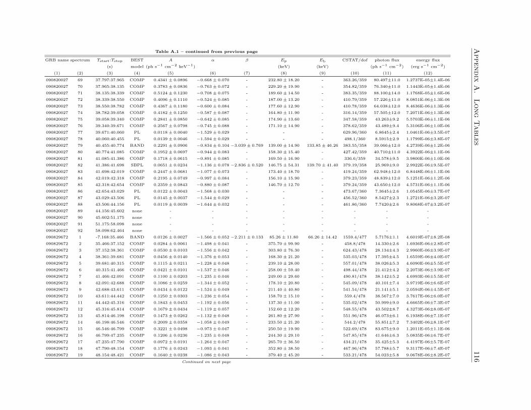
Appendix
A.
Long
Tables
116Table A.1 – continued from previous page
GRB name spectrum Tstart:Tstop BEST A α β Ep Eb CSTAT/dof photon flux energy flux
(s) model (ph s−1 cm−2 keV−1) (keV) (keV) (ph s−1 cm−2) (erg s−1 cm−2)
(1) (2) (3) (4) (5) (6) (7) (8) (9) (10) (11) (12)
090820027 69 37.797:37.965 COMP 0.4341± 0.0896 −0.668± 0.070 - 232.80± 18.20 - 363.26/359 80.497±11.0 1.2737E-05±1.4E-06
090820027 70 37.965:38.135 COMP 0.3783± 0.0836 −0.763± 0.072 - 229.20± 19.90 - 354.82/359 76.340±11.0 1.1443E-05±1.4E-06
090820027 71 38.135:38.339 COMP 0.5124± 0.1230 −0.708± 0.075 - 189.60± 14.50 - 383.35/359 88.100±14.0 1.1768E-05±1.6E-06
090820027 72 38.339:38.550 COMP 0.4096± 0.1110 −0.524± 0.085 - 187.00± 13.20 - 410.79/359 57.226±11.0 8.0851E-06±1.3E-06
090820027 73 38.550:38.782 COMP 0.4367± 0.1180 −0.600± 0.084 - 177.60± 12.90 - 410.78/359 64.038±12.0 8.4636E-06±1.3E-06
090820027 74 38.782:39.058 COMP 0.4182± 0.1250 −0.587± 0.087 - 164.80± 11.90 - 316.14/359 57.505±12.0 7.2071E-06±1.3E-06
090820027 75 39.058:39.340 COMP 0.2841± 0.0850 −0.642± 0.085 - 174.90± 13.60 - 347.58/359 43.263±9.2 5.5703E-06±1.1E-06
090820027 76 39.340:39.671 COMP 0.2567± 0.0798 −0.745± 0.088 - 171.10± 14.90 - 378.62/359 43.489±9.4 5.3106E-06±1.0E-06
090820027 77 39.671:40.060 PL 0.0118± 0.0040 −1.529± 0.029 - - - 629.96/360 6.8645±2.4 1.0461E-06±3.5E-07
090820027 78 40.060:40.455 PL 0.0139± 0.0046 −1.594± 0.029 - - - 498.1/360 8.5915±2.9 1.1799E-06±3.8E-07
090820027 79 40.455:40.774 BAND 0.2291± 0.0906 −0.834± 0.104 −3.039± 0.769 139.00± 14.90 133.85± 46.26 383.55/358 39.066±12.0 4.2739E-06±1.2E-06
090820027 80 40.774:41.085 COMP 0.1952± 0.0697 −0.944± 0.083 - 158.30± 15.40 - 427.42/359 40.710±11.0 4.3922E-06±1.1E-06
090820027 81 41.085:41.386 COMP 0.1718± 0.0615 −0.891± 0.085 - 169.50± 16.90 - 336.6/359 34.578±9.5 3.9800E-06±1.0E-06
090820027 82 41.386:41.698 SBPL 0.0651± 0.0234 −1.136± 0.078 −2.836± 0.520 146.75± 54.31 139.70± 41.40 379.19/358 25.969±9.0 2.9922E-06±9.5E-07
090820027 83 41.698:42.019 COMP 0.2447± 0.0681 −1.077± 0.073 - 173.40± 18.70 - 419.24/359 62.948±12.0 6.8448E-06±1.1E-06
090820027 84 42.019:42.318 COMP 0.2195± 0.0749 −0.997± 0.084 - 156.10± 15.90 - 379.23/359 48.839±12.0 5.1251E-06±1.2E-06
090820027 85 42.318:42.654 COMP 0.2359± 0.0843 −0.880± 0.087 - 146.70± 12.70 - 379.24/359 43.650±12.0 4.5731E-06±1.1E-06
090820027 86 42.654:43.029 PL 0.0122± 0.0043 −1.568± 0.030 - - - 473.67/360 7.3645±2.6 1.0545E-06±3.7E-07
090820027 87 43.029:43.506 PL 0.0145± 0.0037 −1.544± 0.029 - - - 456.52/360 8.5427±2.3 1.2721E-06±3.2E-07
090820027 88 43.506:44.156 PL 0.0119± 0.0039 −1.644± 0.032 - - - 461.86/360 7.7420±2.6 9.8068E-07±3.2E-07
090820027 89 44.156:45.602 none - - - - - - - -
090820027 90 45.602:51.175 none - - - - - - - -
090820027 91 51.175:58.098 none - - - - - - - -
090820027 92 58.098:62.464 none - - - - - - - -
090829672 1 -7.168:35.466 BAND 0.0126± 0.0027 −1.566± 0.052 −2.211± 0.133 85.26± 11.80 66.26± 14.42 1559.4/477 5.7176±1.1 4.6019E-07±8.2E-08
090829672 2 35.466:37.152 COMP 0.0284± 0.0061 −1.498± 0.041 - 375.70± 99.90 - 458.8/478 14.330±2.6 1.6936E-06±2.8E-07
090829672 3 37.152:38.361 COMP 0.0530± 0.0103 −1.556± 0.042 - 303.80± 76.30 - 624.43/478 28.134±4.3 2.9960E-06±3.9E-07
090829672 4 38.361:39.681 COMP 0.0456± 0.0140 −1.376± 0.053 - 168.30± 21.20 - 535.03/478 17.395±4.5 1.6559E-06±4.0E-07
090829672 5 39.681:40.315 COMP 0.1115± 0.0211 −1.228± 0.048 - 239.10± 28.00 - 557.01/478 38.026±5.3 4.6090E-06±5.5E-07
090829672 6 40.315:41.466 COMP 0.0421± 0.0101 −1.537± 0.046 - 258.00± 59.40 - 498.44/478 21.412±4.2 2.2073E-06±3.9E-07
090829672 7 41.466:42.091 COMP 0.1100± 0.0203 −1.235± 0.046 - 249.00± 29.60 - 490.81/478 38.142±5.2 4.6993E-06±5.5E-07
090829672 8 42.091:42.688 COMP 0.1086± 0.0259 −1.344± 0.052 - 178.10± 20.80 - 545.09/478 40.101±7.4 3.9719E-06±6.6E-07
090829672 9 42.688:43.611 COMP 0.0434± 0.0122 −1.524± 0.049 - 211.40± 40.80 - 541.54/478 21.141±5.1 2.0594E-06±4.5E-07
090829672 10 43.611:44.442 COMP 0.1250± 0.0303 −1.236± 0.054 - 158.70± 15.10 - 559.4/478 38.567±7.0 3.7617E-06±6.0E-07
090829672 11 44.442:45.316 COMP 0.1843± 0.0453 −1.192± 0.056 - 137.30± 11.00 - 535.02/478 50.999±9.0 4.6665E-06±7.3E-07
090829672 12 45.316:45.814 COMP 0.1679± 0.0434 −1.119± 0.057 - 152.60± 12.20 - 548.55/478 43.502±8.7 4.3273E-06±8.0E-07
090829672 13 45.814:46.198 COMP 0.1473± 0.0262 −1.132± 0.048 - 261.80± 27.90 - 551.96/478 46.073±6.1 6.1938E-06±7.1E-07
090829672 14 46.198:46.546 COMP 0.2009± 0.0358 −1.058± 0.049 - 233.50± 21.20 - 544.2/478 55.851±7.2 7.3402E-06±8.1E-07
090829672 15 46.546:46.799 COMP 0.3221± 0.0498 −0.973± 0.047 - 250.50± 19.90 - 522.69/478 83.675±9.0 1.2011E-05±1.1E-06
090829672 16 46.799:47.235 COMP 0.1206± 0.0236 −1.235± 0.048 - 244.30± 29.10 - 547.85/478 41.646±6.3 5.0835E-06±6.7E-07
090829672 17 47.235:47.790 COMP 0.0972± 0.0191 −1.264± 0.047 - 265.70± 36.50 - 434.21/478 35.425±5.3 4.4197E-06±5.7E-07
090829672 18 47.790:48.154 COMP 0.1776± 0.0243 −1.093± 0.041 - 352.80± 38.50 - 467.96/478 57.788±5.7 9.3117E-06±7.4E-07
090829672 19 48.154:48.421 COMP 0.1640± 0.0238 −1.086± 0.043 - 379.40± 45.20 - 533.21/478 54.023±5.8 9.0678E-06±8.2E-07
Continued on next page
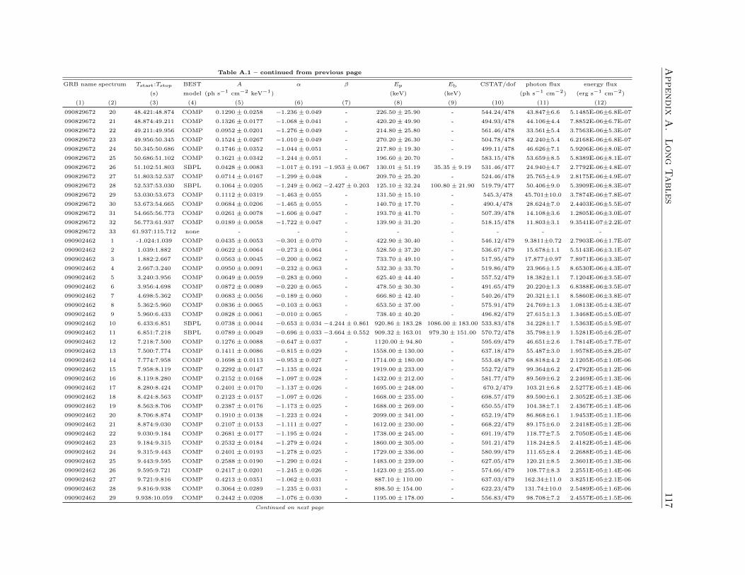
Appendix
A.
Long
Tables
117Table A.1 – continued from previous page
GRB name spectrum Tstart:Tstop BEST A α β Ep Eb CSTAT/dof photon flux energy flux
(s) model (ph s−1 cm−2 keV−1) (keV) (keV) (ph s−1 cm−2) (erg s−1 cm−2)
(1) (2) (3) (4) (5) (6) (7) (8) (9) (10) (11) (12)
090829672 20 48.421:48.874 COMP 0.1290± 0.0258 −1.236± 0.049 - 226.50± 25.90 - 544.24/478 43.847±6.6 5.1485E-06±6.8E-07
090829672 21 48.874:49.211 COMP 0.1326± 0.0177 −1.068± 0.041 - 420.20± 49.90 - 494.93/478 44.106±4.4 7.8852E-06±6.7E-07
090829672 22 49.211:49.956 COMP 0.0952± 0.0201 −1.276± 0.049 - 214.80± 25.80 - 561.46/478 33.561±5.4 3.7563E-06±5.3E-07
090829672 23 49.956:50.345 COMP 0.1524± 0.0267 −1.010± 0.049 - 270.20± 26.30 - 504.78/478 42.240±5.4 6.2168E-06±6.8E-07
090829672 24 50.345:50.686 COMP 0.1746± 0.0352 −1.044± 0.051 - 217.80± 19.30 - 499.11/478 46.626±7.1 5.9206E-06±8.0E-07
090829672 25 50.686:51.102 COMP 0.1621± 0.0342 −1.244± 0.051 - 196.60± 20.70 - 583.15/478 53.659±8.5 5.8389E-06±8.1E-07
090829672 26 51.102:51.803 SBPL 0.0428± 0.0083 −1.017± 0.191 −1.953± 0.067 130.01± 51.19 35.35± 9.19 531.46/477 24.940±4.7 2.7792E-06±4.8E-07
090829672 27 51.803:52.537 COMP 0.0714± 0.0167 −1.299± 0.048 - 209.70± 25.20 - 524.46/478 25.765±4.9 2.8175E-06±4.9E-07
090829672 28 52.537:53.030 SBPL 0.1064± 0.0205 −1.249± 0.062 −2.427± 0.203 125.10± 32.24 100.80± 21.90 519.79/477 50.406±9.0 5.3909E-06±8.3E-07
090829672 29 53.030:53.673 COMP 0.1112± 0.0319 −1.463± 0.055 - 131.50± 15.10 - 545.3/478 45.701±10.0 3.7874E-06±7.8E-07
090829672 30 53.673:54.665 COMP 0.0684± 0.0206 −1.465± 0.055 - 140.70± 17.70 - 490.4/478 28.624±7.0 2.4403E-06±5.5E-07
090829672 31 54.665:56.773 COMP 0.0261± 0.0078 −1.606± 0.047 - 193.70± 41.70 - 507.39/478 14.108±3.6 1.2805E-06±3.0E-07
090829672 32 56.773:61.937 COMP 0.0189± 0.0058 −1.722± 0.047 - 139.90± 31.20 - 518.15/478 11.803±3.1 9.3541E-07±2.2E-07
090829672 33 61.937:115.712 none - - - - - - - -
090902462 1 -1.024:1.039 COMP 0.0435± 0.0053 −0.301± 0.070 - 422.90± 30.40 - 546.12/479 9.3811±0.72 2.7903E-06±1.7E-07
090902462 2 1.039:1.882 COMP 0.0622± 0.0064 −0.273± 0.064 - 528.50± 37.20 - 536.67/479 15.678±1.1 5.5143E-06±3.1E-07
090902462 3 1.882:2.667 COMP 0.0563± 0.0045 −0.200± 0.062 - 733.70± 49.10 - 517.95/479 17.877±0.97 7.8971E-06±3.3E-07
090902462 4 2.667:3.240 COMP 0.0950± 0.0091 −0.232± 0.063 - 532.30± 33.70 - 519.86/479 23.966±1.5 8.6530E-06±4.3E-07
090902462 5 3.240:3.956 COMP 0.0649± 0.0059 −0.283± 0.060 - 625.40± 44.40 - 557.52/479 18.382±1.1 7.1204E-06±3.5E-07
090902462 6 3.956:4.698 COMP 0.0872± 0.0089 −0.220± 0.065 - 478.50± 30.30 - 491.65/479 20.220±1.3 6.8388E-06±3.5E-07
090902462 7 4.698:5.362 COMP 0.0683± 0.0056 −0.189± 0.060 - 666.80± 42.40 - 540.26/479 20.321±1.1 8.5860E-06±3.8E-07
090902462 8 5.362:5.960 COMP 0.0836± 0.0065 −0.103± 0.063 - 653.50± 37.00 - 575.91/479 24.769±1.3 1.0813E-05±4.3E-07
090902462 9 5.960:6.433 COMP 0.0828± 0.0061 −0.010± 0.065 - 738.40± 40.20 - 496.82/479 27.615±1.3 1.3468E-05±5.0E-07
090902462 10 6.433:6.851 SBPL 0.0738± 0.0044 −0.653± 0.034 −4.244± 0.861 920.86± 183.28 1086.00± 183.00 533.83/478 34.228±1.7 1.5363E-05±5.9E-07
090902462 11 6.851:7.218 SBPL 0.0789± 0.0049 −0.696± 0.033 −3.664± 0.552 909.32± 163.01 979.30± 151.00 570.72/478 35.798±1.9 1.5281E-05±6.2E-07
090902462 12 7.218:7.500 COMP 0.1276± 0.0088 −0.647± 0.037 - 1120.00± 94.80 - 595.69/479 46.651±2.6 1.7814E-05±7.7E-07
090902462 13 7.500:7.774 COMP 0.1411± 0.0086 −0.815± 0.029 - 1558.00± 130.00 - 637.18/479 55.487±3.0 1.9578E-05±8.2E-07
090902462 14 7.774:7.958 COMP 0.1698± 0.0113 −0.953± 0.027 - 1714.00± 180.00 - 553.48/479 68.818±4.2 2.1205E-05±1.0E-06
090902462 15 7.958:8.119 COMP 0.2292± 0.0147 −1.135± 0.024 - 1919.00± 233.00 - 552.72/479 99.364±6.2 2.4792E-05±1.2E-06
090902462 16 8.119:8.280 COMP 0.2152± 0.0168 −1.097± 0.028 - 1432.00± 212.00 - 581.77/479 89.569±6.2 2.2469E-05±1.3E-06
090902462 17 8.280:8.424 COMP 0.2401± 0.0170 −1.137± 0.026 - 1695.00± 248.00 - 670.2/479 103.21±6.8 2.5277E-05±1.4E-06
090902462 18 8.424:8.563 COMP 0.2123± 0.0157 −1.097± 0.026 - 1668.00± 235.00 - 698.57/479 89.590±6.1 2.3052E-05±1.3E-06
090902462 19 8.563:8.706 COMP 0.2387± 0.0176 −1.173± 0.025 - 1688.00± 269.00 - 650.55/479 104.38±7.1 2.4367E-05±1.4E-06
090902462 20 8.706:8.874 COMP 0.1910± 0.0138 −1.223± 0.024 - 2099.00± 341.00 - 652.19/479 86.868±6.1 1.9453E-05±1.1E-06
090902462 21 8.874:9.030 COMP 0.2107± 0.0153 −1.111± 0.027 - 1612.00± 230.00 - 668.22/479 89.175±6.0 2.2418E-05±1.2E-06
090902462 22 9.030:9.184 COMP 0.2681± 0.0177 −1.195± 0.024 - 1738.00± 245.00 - 691.19/479 118.77±7.5 2.7050E-05±1.4E-06
090902462 23 9.184:9.315 COMP 0.2532± 0.0184 −1.279± 0.024 - 1860.00± 305.00 - 591.21/479 118.24±8.5 2.4182E-05±1.4E-06
090902462 24 9.315:9.443 COMP 0.2401± 0.0193 −1.278± 0.025 - 1729.00± 336.00 - 580.99/479 111.65±8.4 2.2688E-05±1.4E-06
090902462 25 9.443:9.595 COMP 0.2588± 0.0190 −1.290± 0.024 - 1483.00± 239.00 - 627.05/479 120.21±8.5 2.3601E-05±1.3E-06
090902462 26 9.595:9.721 COMP 0.2417± 0.0201 −1.245± 0.026 - 1423.00± 255.00 - 574.66/479 108.77±8.3 2.2551E-05±1.4E-06
090902462 27 9.721:9.816 COMP 0.4213± 0.0351 −1.062± 0.031 - 887.10± 110.00 - 637.03/479 162.34±11.0 3.8251E-05±2.1E-06
090902462 28 9.816:9.938 COMP 0.3064± 0.0289 −1.235± 0.031 - 898.50± 154.00 - 622.23/479 131.74±10.0 2.5489E-05±1.6E-06
090902462 29 9.938:10.059 COMP 0.2442± 0.0208 −1.076± 0.030 - 1195.00± 178.00 - 556.83/479 98.708±7.2 2.4557E-05±1.5E-06
Continued on next page
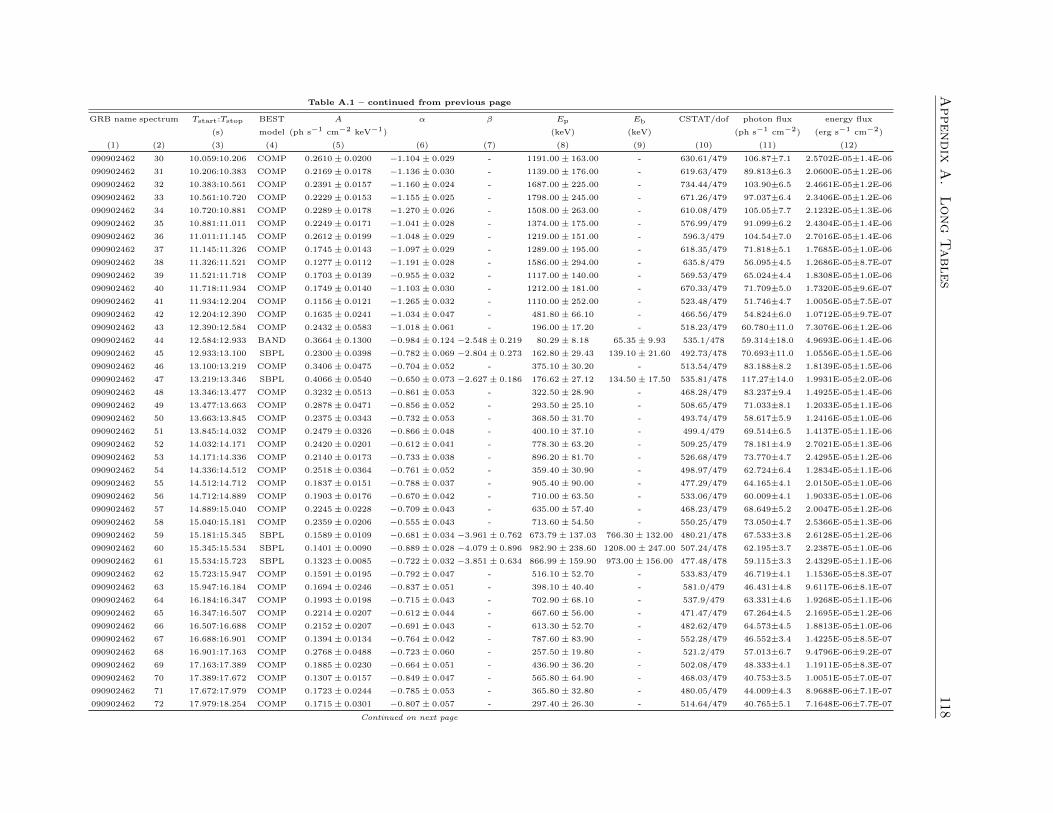
Appendix
A.
Long
Tables
118Table A.1 – continued from previous page
GRB name spectrum Tstart:Tstop BEST A α β Ep Eb CSTAT/dof photon flux energy flux
(s) model (ph s−1 cm−2 keV−1) (keV) (keV) (ph s−1 cm−2) (erg s−1 cm−2)
(1) (2) (3) (4) (5) (6) (7) (8) (9) (10) (11) (12)
090902462 30 10.059:10.206 COMP 0.2610± 0.0200 −1.104± 0.029 - 1191.00± 163.00 - 630.61/479 106.87±7.1 2.5702E-05±1.4E-06
090902462 31 10.206:10.383 COMP 0.2169± 0.0178 −1.136± 0.030 - 1139.00± 176.00 - 619.63/479 89.813±6.3 2.0600E-05±1.2E-06
090902462 32 10.383:10.561 COMP 0.2391± 0.0157 −1.160± 0.024 - 1687.00± 225.00 - 734.44/479 103.90±6.5 2.4661E-05±1.2E-06
090902462 33 10.561:10.720 COMP 0.2229± 0.0153 −1.155± 0.025 - 1798.00± 245.00 - 671.26/479 97.037±6.4 2.3406E-05±1.2E-06
090902462 34 10.720:10.881 COMP 0.2289± 0.0178 −1.270± 0.026 - 1508.00± 263.00 - 610.08/479 105.05±7.7 2.1232E-05±1.3E-06
090902462 35 10.881:11.011 COMP 0.2249± 0.0171 −1.041± 0.028 - 1374.00± 175.00 - 576.99/479 91.099±6.2 2.4304E-05±1.4E-06
090902462 36 11.011:11.145 COMP 0.2612± 0.0199 −1.048± 0.029 - 1219.00± 151.00 - 596.3/479 104.54±7.0 2.7016E-05±1.4E-06
090902462 37 11.145:11.326 COMP 0.1745± 0.0143 −1.097± 0.029 - 1289.00± 195.00 - 618.35/479 71.818±5.1 1.7685E-05±1.0E-06
090902462 38 11.326:11.521 COMP 0.1277± 0.0112 −1.191± 0.028 - 1586.00± 294.00 - 635.8/479 56.095±4.5 1.2686E-05±8.7E-07
090902462 39 11.521:11.718 COMP 0.1703± 0.0139 −0.955± 0.032 - 1117.00± 140.00 - 569.53/479 65.024±4.4 1.8308E-05±1.0E-06
090902462 40 11.718:11.934 COMP 0.1749± 0.0140 −1.103± 0.030 - 1212.00± 181.00 - 670.33/479 71.709±5.0 1.7320E-05±9.6E-07
090902462 41 11.934:12.204 COMP 0.1156± 0.0121 −1.265± 0.032 - 1110.00± 252.00 - 523.48/479 51.746±4.7 1.0056E-05±7.5E-07
090902462 42 12.204:12.390 COMP 0.1635± 0.0241 −1.034± 0.047 - 481.80± 66.10 - 466.56/479 54.824±6.0 1.0712E-05±9.7E-07
090902462 43 12.390:12.584 COMP 0.2432± 0.0583 −1.018± 0.061 - 196.00± 17.20 - 518.23/479 60.780±11.0 7.3076E-06±1.2E-06
090902462 44 12.584:12.933 BAND 0.3664± 0.1300 −0.984± 0.124 −2.548± 0.219 80.29± 8.18 65.35± 9.93 535.1/478 59.314±18.0 4.9693E-06±1.4E-06
090902462 45 12.933:13.100 SBPL 0.2300± 0.0398 −0.782± 0.069 −2.804± 0.273 162.80± 29.43 139.10± 21.60 492.73/478 70.693±11.0 1.0556E-05±1.5E-06
090902462 46 13.100:13.219 COMP 0.3406± 0.0475 −0.704± 0.052 - 375.10± 30.20 - 513.54/479 83.188±8.2 1.8139E-05±1.5E-06
090902462 47 13.219:13.346 SBPL 0.4066± 0.0540 −0.650± 0.073 −2.627± 0.186 176.62± 27.12 134.50± 17.50 535.81/478 117.27±14.0 1.9931E-05±2.0E-06
090902462 48 13.346:13.477 COMP 0.3232± 0.0513 −0.861± 0.053 - 322.50± 28.90 - 468.28/479 83.237±9.4 1.4925E-05±1.4E-06
090902462 49 13.477:13.663 COMP 0.2878± 0.0471 −0.856± 0.052 - 293.50± 25.10 - 508.65/479 71.033±8.1 1.2033E-05±1.1E-06
090902462 50 13.663:13.845 COMP 0.2375± 0.0343 −0.732± 0.053 - 368.50± 31.70 - 493.74/479 58.617±5.9 1.2416E-05±1.0E-06
090902462 51 13.845:14.032 COMP 0.2479± 0.0326 −0.866± 0.048 - 400.10± 37.10 - 499.4/479 69.514±6.5 1.4137E-05±1.1E-06
090902462 52 14.032:14.171 COMP 0.2420± 0.0201 −0.612± 0.041 - 778.30± 63.20 - 509.25/479 78.181±4.9 2.7021E-05±1.3E-06
090902462 53 14.171:14.336 COMP 0.2140± 0.0173 −0.733± 0.038 - 896.20± 81.70 - 526.68/479 73.770±4.7 2.4295E-05±1.2E-06
090902462 54 14.336:14.512 COMP 0.2518± 0.0364 −0.761± 0.052 - 359.40± 30.90 - 498.97/479 62.724±6.4 1.2834E-05±1.1E-06
090902462 55 14.512:14.712 COMP 0.1837± 0.0151 −0.788± 0.037 - 905.40± 90.00 - 477.29/479 64.165±4.1 2.0150E-05±1.0E-06
090902462 56 14.712:14.889 COMP 0.1903± 0.0176 −0.670± 0.042 - 710.00± 63.50 - 533.06/479 60.009±4.1 1.9033E-05±1.0E-06
090902462 57 14.889:15.040 COMP 0.2245± 0.0228 −0.709± 0.043 - 635.00± 57.40 - 468.23/479 68.649±5.2 2.0047E-05±1.2E-06
090902462 58 15.040:15.181 COMP 0.2359± 0.0206 −0.555± 0.043 - 713.60± 54.50 - 550.25/479 73.050±4.7 2.5366E-05±1.3E-06
090902462 59 15.181:15.345 SBPL 0.1589± 0.0109 −0.681± 0.034 −3.961± 0.762 673.79± 137.03 766.30± 132.00 480.21/478 67.533±3.8 2.6128E-05±1.2E-06
090902462 60 15.345:15.534 SBPL 0.1401± 0.0090 −0.889± 0.028 −4.079± 0.896 982.90± 238.60 1208.00± 247.00 507.24/478 62.195±3.7 2.2387E-05±1.0E-06
090902462 61 15.534:15.723 SBPL 0.1323± 0.0085 −0.722± 0.032 −3.851± 0.634 866.99± 159.90 973.00± 156.00 477.48/478 59.115±3.3 2.4329E-05±1.1E-06
090902462 62 15.723:15.947 COMP 0.1591± 0.0195 −0.792± 0.047 - 516.10± 52.70 - 533.83/479 46.719±4.1 1.1536E-05±8.3E-07
090902462 63 15.947:16.184 COMP 0.1694± 0.0246 −0.837± 0.051 - 398.10± 40.40 - 581.0/479 46.431±4.8 9.6117E-06±8.1E-07
090902462 64 16.184:16.347 COMP 0.1993± 0.0198 −0.715± 0.043 - 702.90± 68.10 - 537.9/479 63.331±4.6 1.9268E-05±1.1E-06
090902462 65 16.347:16.507 COMP 0.2214± 0.0207 −0.612± 0.044 - 667.60± 56.00 - 471.47/479 67.264±4.5 2.1695E-05±1.2E-06
090902462 66 16.507:16.688 COMP 0.2152± 0.0207 −0.691± 0.043 - 613.30± 52.70 - 482.62/479 64.573±4.5 1.8813E-05±1.0E-06
090902462 67 16.688:16.901 COMP 0.1394± 0.0134 −0.764± 0.042 - 787.60± 83.90 - 552.28/479 46.552±3.4 1.4225E-05±8.5E-07
090902462 68 16.901:17.163 COMP 0.2768± 0.0488 −0.723± 0.060 - 257.50± 19.80 - 521.2/479 57.013±6.7 9.4796E-06±9.2E-07
090902462 69 17.163:17.389 COMP 0.1885± 0.0230 −0.664± 0.051 - 436.90± 36.20 - 502.08/479 48.333±4.1 1.1911E-05±8.3E-07
090902462 70 17.389:17.672 COMP 0.1307± 0.0157 −0.849± 0.047 - 565.80± 64.90 - 468.03/479 40.753±3.5 1.0051E-05±7.0E-07
090902462 71 17.672:17.979 COMP 0.1723± 0.0244 −0.785± 0.053 - 365.80± 32.80 - 480.05/479 44.009±4.3 8.9688E-06±7.1E-07
090902462 72 17.979:18.254 COMP 0.1715± 0.0301 −0.807± 0.057 - 297.40± 26.30 - 514.64/479 40.765±5.1 7.1648E-06±7.7E-07
Continued on next page
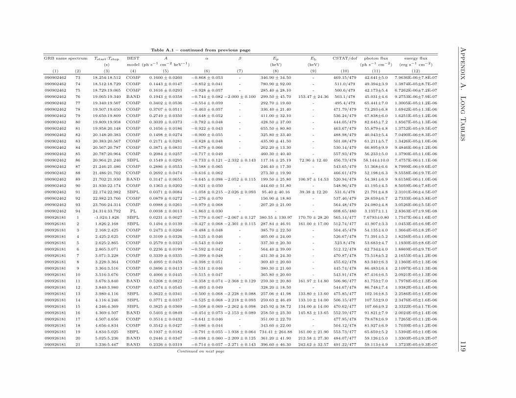
Appendix
A.
Long
Tables
119Table A.1 – continued from previous page
GRB name spectrum Tstart:Tstop BEST A α β Ep Eb CSTAT/dof photon flux energy flux
(s) model (ph s−1 cm−2 keV−1) (keV) (keV) (ph s−1 cm−2) (erg s−1 cm−2)
(1) (2) (3) (4) (5) (6) (7) (8) (9) (10) (11) (12)
090902462 73 18.254:18.512 COMP 0.1600± 0.0260 −0.868± 0.053 - 346.90± 34.50 - 469.15/479 42.641±5.0 7.9636E-06±7.8E-07
090902462 74 18.512:18.729 COMP 0.1443± 0.0147 −0.852± 0.041 - 780.90± 92.00 - 511.0/479 49.394±3.9 1.3874E-05±8.7E-07
090902462 75 18.729:19.065 COMP 0.1616± 0.0293 −0.928± 0.057 - 285.40± 28.10 - 500.6/479 42.173±5.4 6.7262E-06±7.2E-07
090902462 76 19.065:19.340 BAND 0.1943± 0.0358 −0.744± 0.082 −2.000± 0.100 299.50± 45.70 153.47± 24.36 503.1/478 45.031±4.6 9.2753E-06±7.9E-07
090902462 77 19.340:19.507 COMP 0.3402± 0.0536 −0.554± 0.059 - 292.70± 19.60 - 495.4/479 65.441±7.0 1.3005E-05±1.2E-06
090902462 78 19.507:19.650 COMP 0.3707± 0.0511 −0.463± 0.057 - 336.40± 21.40 - 471.79/479 73.293±6.8 1.6942E-05±1.3E-06
090902462 79 19.650:19.809 COMP 0.2749± 0.0350 −0.648± 0.052 - 411.00± 32.10 - 536.24/479 67.838±6.0 1.6251E-05±1.2E-06
090902462 80 19.809:19.958 COMP 0.3039± 0.0373 −0.782± 0.048 - 428.50± 37.00 - 444.05/479 82.645±7.2 1.8567E-05±1.3E-06
090902462 81 19.958:20.148 COMP 0.1656± 0.0186 −0.922± 0.043 - 655.50± 80.80 - 463.67/479 55.879±4.8 1.3752E-05±9.5E-07
090902462 82 20.148:20.383 COMP 0.1498± 0.0274 −0.900± 0.055 - 325.80± 33.40 - 488.98/479 40.043±5.4 7.0490E-06±8.3E-07
090902462 83 20.383:20.567 COMP 0.2171± 0.0281 −0.828± 0.048 - 435.90± 41.50 - 501.08/479 61.211±5.7 1.3426E-05±1.0E-06
090902462 84 20.567:20.787 COMP 0.3871± 0.0831 −0.679± 0.066 - 202.20± 13.30 - 530.14/479 66.895±9.9 9.4846E-06±1.2E-06
090902462 85 20.787:20.964 COMP 0.2084± 0.0257 −0.717± 0.049 - 460.30± 40.40 - 557.93/479 56.233±5.0 1.3790E-05±1.0E-06
090902462 86 20.964:21.246 SBPL 0.1549± 0.0295 −0.733± 0.121 −2.332± 0.143 117.16± 25.19 72.96± 12.40 456.73/478 58.144±10.0 7.4757E-06±1.1E-06
090902462 87 21.246:21.486 COMP 0.2886± 0.0553 −0.588± 0.065 - 246.40± 17.30 - 543.65/479 51.368±6.6 8.7999E-06±9.6E-07
090902462 88 21.486:21.702 COMP 0.2692± 0.0474 −0.616± 0.062 - 273.30± 19.90 - 466.61/479 52.198±6.3 9.5558E-06±9.7E-07
090902462 89 21.702:21.930 BAND 0.3147± 0.0655 −0.645± 0.098 −2.052± 0.115 199.50± 25.80 106.97± 14.53 520.94/478 54.381±6.9 9.6158E-06±1.0E-06
090902462 90 21.930:22.174 COMP 0.1363± 0.0202 −0.921± 0.050 - 444.60± 51.80 - 548.96/479 41.195±4.5 8.5059E-06±7.8E-07
090902462 91 22.174:22.982 SBPL 0.0371± 0.0084 −1.058± 0.215 −2.026± 0.093 95.40± 40.16 39.38± 12.20 531.6/478 21.791±4.8 2.3101E-06±4.5E-07
090902462 92 22.982:23.766 COMP 0.0879± 0.0272 −1.276± 0.070 - 156.90± 18.80 - 537.46/479 28.659±6.7 2.7333E-06±5.8E-07
090902462 93 23.766:24.314 COMP 0.0988± 0.0261 −0.979± 0.068 - 207.20± 21.00 - 564.48/479 24.080±4.8 3.0526E-06±5.5E-07
090902462 94 24.314:33.792 PL 0.0038± 0.0013 −1.863± 0.030 - - - 608.65/480 3.1357±1.1 2.8363E-07±9.9E-08
090926181 1 -1.024:1.826 SBPL 0.0231± 0.0027 −0.779± 0.067 −2.067± 0.127 380.55± 130.97 170.70± 28.20 565.14/477 7.6793±0.80 1.7547E-06±1.6E-07
090926181 2 1.826:2.168 SBPL 0.1494± 0.0139 −0.427± 0.068 −2.301± 0.115 287.84± 46.91 161.00± 17.00 512.74/477 41.907±3.3 1.0453E-05±6.9E-07
090926181 3 2.168:2.425 COMP 0.2473± 0.0266 −0.488± 0.048 - 385.70± 22.50 - 504.45/478 54.135±4.0 1.3664E-05±8.2E-07
090926181 4 2.425:2.625 COMP 0.3109± 0.0326 −0.525± 0.046 - 405.00± 24.00 - 526.67/478 71.391±5.2 1.8256E-05±1.0E-06
090926181 5 2.625:2.865 COMP 0.2579± 0.0323 −0.543± 0.049 - 337.30± 20.30 - 523.8/478 53.683±4.7 1.1930E-05±8.6E-07
090926181 6 2.865:3.071 COMP 0.2236± 0.0199 −0.592± 0.042 - 564.40± 39.00 - 512.12/478 62.734±4.0 1.8869E-05±9.7E-07
090926181 7 3.071:3.228 COMP 0.3339± 0.0335 −0.399± 0.048 - 431.30± 24.30 - 470.87/478 75.518±5.2 2.1655E-05±1.2E-06
090926181 8 3.228:3.364 COMP 0.4095± 0.0459 −0.398± 0.051 - 369.40± 20.60 - 455.62/478 83.340±6.3 2.1360E-05±1.3E-06
090926181 9 3.364:3.516 COMP 0.3896± 0.0413 −0.531± 0.046 - 380.30± 21.60 - 445.74/478 86.483±6.4 2.1097E-05±1.3E-06
090926181 10 3.516:3.676 COMP 0.4066± 0.0445 −0.515± 0.047 - 365.80± 20.60 - 543.91/478 87.416±6.5 2.0921E-05±1.3E-06
090926181 11 3.676:3.840 BAND 0.5208± 0.0822 −0.358± 0.074 −2.368± 0.129 259.30± 20.80 161.97± 14.80 506.96/477 81.753±7.0 1.7978E-05±1.3E-06
090926181 12 3.840:3.980 COMP 0.4374± 0.0545 −0.493± 0.049 - 328.20± 18.50 - 544.67/478 86.748±7.4 1.9382E-05±1.4E-06
090926181 13 3.980:4.116 SBPL 0.3622± 0.0341 −0.500± 0.068 −2.228± 0.088 257.06± 41.98 133.80± 13.60 475.85/477 102.16±8.5 2.2586E-05±1.6E-06
090926181 14 4.116:4.246 SBPL 0.3771± 0.0357 −0.525± 0.068 −2.218± 0.093 259.63± 46.49 133.10± 14.00 506.15/477 107.53±9.0 2.3476E-05±1.6E-06
090926181 15 4.246:4.369 SBPL 0.3825± 0.0369 −0.508± 0.069 −2.262± 0.098 245.92± 38.72 134.00± 14.00 470.62/477 107.66±9.2 2.3322E-05±1.7E-06
090926181 16 4.369:4.507 BAND 0.5403± 0.0849 −0.454± 0.073 −2.153± 0.089 258.50± 23.30 145.83± 13.65 552.59/477 91.821±7.9 2.0024E-05±1.4E-06
090926181 17 4.507:4.656 COMP 0.3514± 0.0432 −0.641± 0.046 - 351.00± 22.70 - 477.95/478 79.678±6.9 1.7265E-05±1.2E-06
090926181 18 4.656:4.834 COMP 0.3542± 0.0427 −0.686± 0.044 - 343.60± 22.00 - 504.12/478 81.927±6.9 1.7039E-05±1.2E-06
090926181 19 4.834:5.025 SBPL 0.1937± 0.0182 −0.791± 0.055 −1.938± 0.064 734.41± 264.88 161.00± 21.90 553.73/477 65.659±5.2 1.5394E-05±1.0E-06
090926181 20 5.025:5.236 BAND 0.2446± 0.0347 −0.698± 0.060 −2.209± 0.125 361.20± 41.90 212.58± 27.30 484.07/477 59.126±5.0 1.3303E-05±9.2E-07
090926181 21 5.236:5.447 BAND 0.2326± 0.0319 −0.714± 0.057 −2.271± 0.143 396.60± 46.30 242.62± 32.57 491.22/477 59.113±4.9 1.3723E-05±9.3E-07
Continued on next page
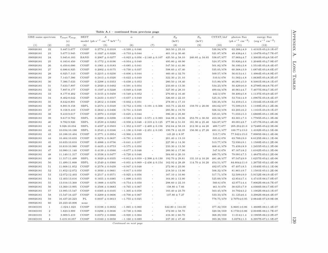
Appendix
A.
Long
Tables
120Table A.1 – continued from previous page
GRB name spectrum Tstart:Tstop BEST A α β Ep Eb CSTAT/dof photon flux energy flux
(s) model (ph s−1 cm−2 keV−1) (keV) (keV) (ph s−1 cm−2) (erg s−1 cm−2)
(1) (2) (3) (4) (5) (6) (7) (8) (9) (10) (11) (12)
090926181 22 5.447:5.677 COMP 0.2774± 0.0318 −0.599± 0.046 - 363.50± 23.10 - 536.94/478 62.388±4.9 1.4191E-05±9.1E-07
090926181 23 5.677:5.945 COMP 0.1927± 0.0226 −0.733± 0.044 - 401.10± 30.40 - 521.87/478 49.438±4.1 1.1047E-05±7.7E-07
090926181 24 5.945:6.183 BAND 0.2067± 0.0277 −0.823± 0.056 −2.140± 0.107 425.50± 58.10 240.85± 34.65 538.67/477 57.969±4.7 1.3003E-05±8.5E-07
090926181 25 6.183:6.450 COMP 0.1772± 0.0196 −0.934± 0.040 - 495.80± 49.90 - 524.37/478 55.826±4.6 1.2046E-05±7.9E-07
090926181 26 6.450:6.686 COMP 0.1961± 0.0183 −0.685± 0.041 - 547.50± 41.90 - 501.82/478 56.100±3.8 1.5514E-05±8.4E-07
090926181 27 6.686:6.925 COMP 0.2002± 0.0175 −0.730± 0.037 - 598.60± 47.40 - 535.05/478 60.368±3.9 1.6874E-05±8.6E-07
090926181 28 6.925:7.143 COMP 0.2215± 0.0230 −0.606± 0.044 - 460.40± 32.70 - 509.57/478 56.613±4.1 1.4984E-05±8.9E-07
090926181 29 7.143:7.386 COMP 0.2413± 0.0320 −0.622± 0.049 - 322.30± 21.10 - 510.0/478 51.582±4.8 1.0636E-05±8.3E-07
090926181 30 7.386:7.633 COMP 0.2298± 0.0353 −0.638± 0.053 - 280.50± 18.40 - 515.89/478 46.081±5.0 8.5081E-06±8.1E-07
090926181 31 7.633:7.897 COMP 0.2920± 0.0492 −0.591± 0.054 - 233.60± 13.30 - 534.23/478 50.429±6.0 8.2798E-06±8.7E-07
090926181 32 7.897:8.177 COMP 0.1597± 0.0248 −0.849± 0.048 - 327.00± 28.10 - 499.64/478 40.961±4.7 7.4677E-06±7.3E-07
090926181 33 8.177:8.402 COMP 0.3155± 0.0458 −0.549± 0.052 - 276.60± 16.40 - 442.3/478 58.400±5.8 1.1137E-05±9.4E-07
090926181 34 8.402:8.642 COMP 0.2433± 0.0317 −0.657± 0.049 - 326.60± 22.10 - 525.31/478 53.734±4.9 1.0967E-05±8.4E-07
090926181 35 8.642:8.891 COMP 0.2812± 0.0406 −0.602± 0.051 - 278.00± 17.10 - 530.35/478 54.459±5.4 1.0164E-05±8.6E-07
090926181 36 8.891:9.158 SBPL 0.2574± 0.0349 −0.752± 0.056 −3.191± 0.306 163.75± 22.83 159.70± 20.00 484.62/477 75.599±9.5 1.1189E-05±1.2E-06
090926181 37 9.158:9.410 COMP 0.2842± 0.0406 −0.751± 0.049 - 285.90± 19.70 - 506.52/478 63.205±6.2 1.1161E-05±9.1E-07
090926181 38 9.410:9.617 COMP 0.2970± 0.0320 −0.625± 0.044 - 396.20± 25.80 - 525.61/478 71.033±5.3 1.6869E-05±1.0E-06
090926181 39 9.617:9.782 SBPL 0.2889± 0.0298 −0.585± 0.048 −3.571± 0.393 244.98± 33.06 253.70± 30.50 453.58/477 83.301±7.3 1.7785E-05±1.3E-06
090926181 40 9.782:9.926 SBPL 0.2539± 0.0282 −0.938± 0.048 −2.319± 0.125 277.86± 51.03 181.90± 25.40 524.87/477 89.091±8.7 1.6717E-05±1.4E-06
090926181 41 9.926:10.034 SBPL 0.4337± 0.0503 −1.352± 0.037 −2.409± 0.156 252.64± 58.18 212.30± 44.20 489.7/477 205.29±21.0 2.7248E-05±2.3E-06
090926181 42 10.034:10.188 SBPL 0.2543± 0.0346 −1.136± 0.048 −2.451± 0.185 199.78± 42.35 156.90± 27.20 483.11/477 100.77±13.0 1.4182E-05±1.5E-06
090926181 43 10.188:10.404 COMP 0.3771± 0.0954 −0.966± 0.059 - 145.20± 8.97 - 513.7/478 77.942±15.0 7.8985E-06±1.4E-06
090926181 44 10.404:10.633 COMP 0.3276± 0.0637 −0.791± 0.055 - 201.40± 13.10 - 535.0/478 63.789±9.0 8.6125E-06±1.1E-06
090926181 45 10.633:10.810 COMP 0.4088± 0.0736 −0.641± 0.057 - 227.90± 14.30 - 513.77/478 72.930±9.1 1.1500E-05±1.2E-06
090926181 46 10.810:10.980 COMP 0.4435± 0.0753 −0.575± 0.056 - 233.30± 13.50 - 468.41/478 75.439±8.9 1.2455E-05±1.3E-06
090926181 47 10.980:11.140 COMP 0.4139± 0.0560 −0.677± 0.048 - 289.90± 17.90 - 547.9/478 87.167±8.2 1.6162E-05±1.3E-06
090926181 48 11.140:11.317 COMP 0.3538± 0.0477 −0.720± 0.046 - 304.60± 20.10 - 489.75/478 79.091±7.5 1.4847E-05±1.2E-06
090926181 49 11.317:11.499 SBPL 0.3029± 0.0335 −0.812± 0.059 −2.398± 0.130 192.70± 29.81 131.10± 16.20 481.48/477 97.547±9.9 1.6257E-05±1.4E-06
090926181 50 11.499:11.668 SBPL 0.2549± 0.0360 −0.831± 0.069 −2.436± 0.154 162.92± 28.49 114.70± 16.20 454.51/477 84.604±11.0 1.2675E-05±1.4E-06
090926181 51 11.668:11.852 COMP 0.2578± 0.0439 −0.947± 0.048 - 272.90± 23.00 - 492.07/478 67.407±8.5 1.0340E-05±1.1E-06
090926181 52 11.852:12.072 COMP 0.3930± 0.0661 −0.817± 0.050 - 218.50± 13.90 - 506.32/478 81.861±9.7 1.1581E-05±1.2E-06
090926181 53 12.072:12.403 COMP 0.2517± 0.0571 −0.925± 0.056 - 167.10± 10.80 - 517.71/478 52.509±9.0 5.9152E-06±9.4E-07
090926181 54 12.403:13.016 COMP 0.1655± 0.0385 −1.098± 0.055 - 164.00± 12.90 - 525.69/478 42.854±7.4 4.4741E-06±7.0E-07
090926181 55 13.016:13.360 COMP 0.1888± 0.0276 −0.754± 0.050 - 298.60± 22.10 - 560.6/478 42.977±4.4 7.8062E-06±6.7E-07
090926181 56 13.360:13.995 COMP 0.2506± 0.0683 −0.765± 0.067 - 138.80± 7.66 - 461.9/478 38.625±7.9 4.0366E-06±7.8E-07
090926181 57 13.995:15.547 COMP 0.0305± 0.0105 −1.305± 0.058 - 183.40± 23.70 - 563.45/478 10.792±3.2 1.1002E-06±3.1E-07
090926181 58 15.547:16.437 COMP 0.2209± 0.0606 −0.700± 0.067 - 137.80± 7.27 - 533.33/478 31.125±6.4 3.2982E-06±6.4E-07
090926181 59 16.437:23.223 PL 0.0037± 0.0013 −1.755± 0.025 - - - 778.75/479 2.7070±0.95 2.8844E-07±9.9E-08
090926181 60 23.223:43.008 none - - - - - - - -
091003191 1 -1.024:1.823 COMP 0.0188± 0.0032 −1.065± 0.060 - 642.80± 144.00 - 377.32/359 6.8681±0.86 1.4608E-06±1.4E-07
091003191 2 1.823:3.909 COMP 0.0296± 0.0046 −0.738± 0.066 - 472.00± 58.70 - 320.58/359 8.1750±0.86 2.0049E-06±1.7E-07
091003191 3 3.909:5.419 COMP 0.0372± 0.0068 −0.920± 0.064 - 416.30± 60.70 - 368.29/359 11.014±1.4 2.1995E-06±2.2E-07
091003191 4 5.419:10.057 COMP 0.0160± 0.0058 −1.160± 0.089 - 237.20± 47.40 - 393.26/359 5.0278±1.3 6.2957E-07±1.5E-07
Continued on next page
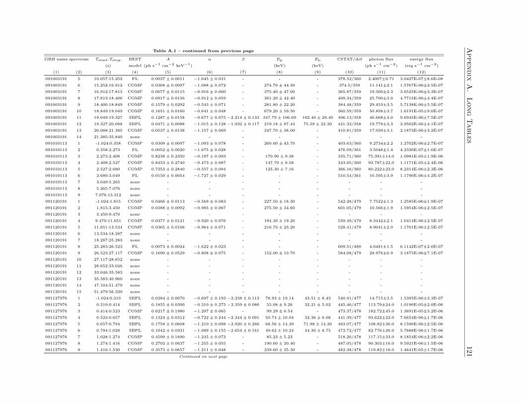
Appendix
A.
Long
Tables
121Table A.1 – continued from previous page
GRB name spectrum Tstart:Tstop BEST A α β Ep Eb CSTAT/dof photon flux energy flux
(s) model (ph s−1 cm−2 keV−1) (keV) (keV) (ph s−1 cm−2) (erg s−1 cm−2)
(1) (2) (3) (4) (5) (6) (7) (8) (9) (10) (11) (12)
091003191 5 10.057:15.252 PL 0.0037± 0.0011 −1.645± 0.031 - - - 378.52/360 2.4007±0.71 3.0427E-07±8.6E-08
091003191 6 15.252:16.912 COMP 0.0368± 0.0097 −1.088± 0.072 - 274.70± 44.30 - 374.5/359 11.141±2.1 1.5767E-06±2.5E-07
091003191 7 16.912:17.813 COMP 0.0677± 0.0115 −0.916± 0.060 - 375.40± 47.00 - 365.87/359 19.300±2.3 3.6525E-06±3.3E-07
091003191 8 17.813:18.406 COMP 0.0917± 0.0156 −0.912± 0.059 - 361.20± 42.40 - 409.34/359 25.700±3.0 4.7715E-06±4.4E-07
091003191 9 18.406:18.849 COMP 0.1579± 0.0292 −0.543± 0.071 - 281.80± 22.20 - 384.48/359 29.453±3.5 5.7138E-06±5.5E-07
091003191 10 18.849:19.049 COMP 0.1651± 0.0160 −0.641± 0.048 - 679.20± 59.50 - 360.59/359 50.858±3.7 1.6191E-05±9.0E-07
091003191 11 19.049:19.327 SBPL 0.1287± 0.0158 −0.677± 0.075 −2.214± 0.133 347.79± 106.69 182.40± 29.40 406.13/358 40.668±4.0 9.6945E-06±7.5E-07
091003191 12 19.327:20.088 SBPL 0.0471± 0.0088 −1.015± 0.128 −1.932± 0.117 219.18± 87.44 75.59± 22.30 421.32/358 19.779±3.3 2.9502E-06±4.1E-07
091003191 13 20.088:21.385 COMP 0.0537± 0.0138 −1.157± 0.069 - 247.70± 38.00 - 410.81/359 17.039±3.1 2.1873E-06±3.2E-07
091003191 14 21.385:35.840 none - - - - - - - -
091010113 1 -1.024:0.358 COMP 0.0309± 0.0097 −1.093± 0.078 - 260.60± 43.70 - 403.63/360 9.2734±2.2 1.2702E-06±2.7E-07
091010113 2 0.358:2.273 PL 0.0052± 0.0020 −1.675± 0.028 - - - 476.09/361 3.5048±1.4 4.2330E-07±1.6E-07
091010113 3 2.273:2.408 COMP 0.8238± 0.2350 −0.187± 0.093 - 170.90± 9.38 - 335.71/360 75.391±14.0 1.0981E-05±1.9E-06
091010113 4 2.408:2.527 COMP 0.8453± 0.2740 −0.473± 0.087 - 147.70± 8.58 - 343.65/360 93.787±22.0 1.1171E-05±2.4E-06
091010113 5 2.527:2.680 COMP 0.7353± 0.2840 −0.557± 0.094 - 125.30± 7.16 - 366.16/360 80.222±23.0 8.2314E-06±2.3E-06
091010113 6 2.680:3.049 PL 0.0150± 0.0054 −1.727± 0.029 - - - 510.54/361 10.595±3.9 1.1790E-06±4.2E-07
091010113 7 3.049:5.265 none - - - - - - - -
091010113 8 5.265:7.076 none - - - - - - - -
091010113 9 7.076:13.312 none - - - - - - - -
091120191 1 -1.024:1.815 COMP 0.0466± 0.0113 −0.569± 0.083 - 227.50± 18.30 - 542.28/479 7.7522±1.3 1.2585E-06±1.9E-07
091120191 2 1.815:3.450 COMP 0.0388± 0.0092 −0.985± 0.067 - 275.50± 34.60 - 601.05/479 10.566±1.9 1.5954E-06±2.5E-07
091120191 3 3.450:9.470 none - - - - - - - -
091120191 4 9.470:11.651 COMP 0.0377± 0.0121 −0.920± 0.076 - 194.30± 19.20 - 539.49/479 8.3442±2.1 1.0414E-06±2.5E-07
091120191 5 11.651:13.534 COMP 0.0365± 0.0106 −0.964± 0.071 - 216.70± 23.20 - 528.41/479 8.9041±2.0 1.1701E-06±2.5E-07
091120191 6 13.534:18.287 none - - - - - - - -
091120191 7 18.287:25.283 none - - - - - - - -
091120191 8 25.283:26.523 PL 0.0073± 0.0024 −1.622± 0.023 - - - 609.51/480 4.6481±1.5 6.1142E-07±2.0E-07
091120191 9 26.523:27.117 COMP 0.1690± 0.0529 −0.808± 0.075 - 152.00± 10.70 - 584.08/479 28.976±6.9 3.1875E-06±7.1E-07
091120191 10 27.117:28.652 none - - - - - - - -
091120191 11 28.652:33.046 none - - - - - - - -
091120191 12 33.046:35.583 none - - - - - - - -
091120191 13 35.583:40.960 none - - - - - - - -
091120191 14 47.104:51.479 none - - - - - - - -
091120191 15 51.479:56.320 none - - - - - - - -
091127976 1 -1.024:0.310 SBPL 0.0284± 0.0070 −0.697± 0.193 −2.238± 0.113 78.93± 19.14 43.51± 8.43 540.91/477 14.715±3.5 1.5395E-06±3.3E-07
091127976 2 0.310:0.414 SBPL 0.1855± 0.0390 −0.310± 0.275 −2.359± 0.086 55.08± 9.26 32.21± 5.02 445.46/477 113.79±24.0 1.0190E-05±2.0E-06
091127976 3 0.414:0.523 COMP 0.6217± 0.1980 −1.297± 0.065 - 99.29± 6.54 - 473.37/478 182.72±45.0 1.3691E-05±3.2E-06
091127976 4 0.523:0.657 SBPL 0.1324± 0.0312 −0.722± 0.244 −2.344± 0.091 50.74± 10.04 32.36± 6.08 441.39/477 93.622±22.0 7.6654E-06±1.7E-06
091127976 5 0.657:0.794 SBPL 0.1758± 0.0608 −1.210± 0.098 −2.920± 0.266 68.56± 14.39 71.98± 14.30 483.07/477 108.82±36.0 8.1590E-06±2.5E-06
091127976 6 0.794:1.028 SBPL 0.1042± 0.0331 −1.089± 0.155 −2.654± 0.161 49.62± 10.24 44.30± 8.75 473.72/477 82.776±26.0 5.7688E-06±1.7E-06
091127976 7 1.028:1.274 COMP 0.4599± 0.1690 −1.245± 0.073 - 85.23± 5.23 - 518.26/478 117.15±33.0 8.1854E-06±2.2E-06
091127976 8 1.274:1.416 COMP 0.2702± 0.0637 −1.255± 0.055 - 190.60± 20.40 - 487.05/478 90.303±16.0 9.5921E-06±1.5E-06
091127976 9 1.416:1.530 COMP 0.3573± 0.0657 −1.211± 0.048 - 239.60± 25.30 - 482.38/478 119.82±16.0 1.4641E-05±1.7E-06
Continued on next page
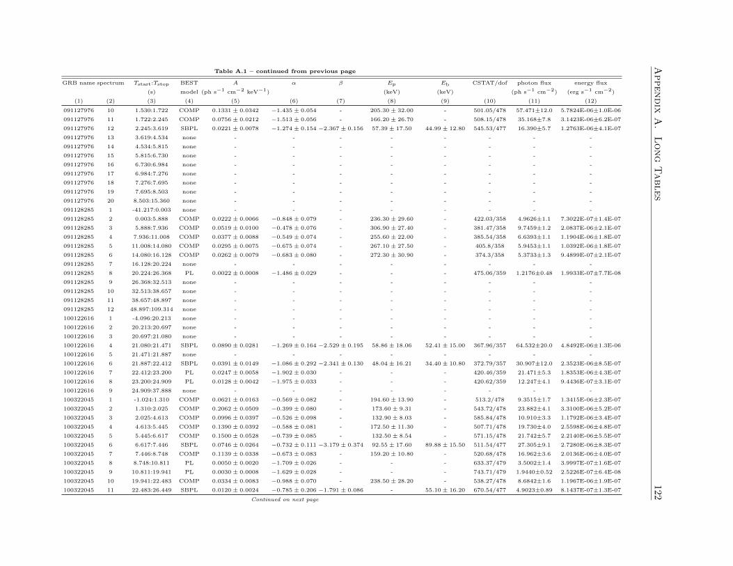
Appendix
A.
Long
Tables
122Table A.1 – continued from previous page
GRB name spectrum Tstart:Tstop BEST A α β Ep Eb CSTAT/dof photon flux energy flux
(s) model (ph s−1 cm−2 keV−1) (keV) (keV) (ph s−1 cm−2) (erg s−1 cm−2)
(1) (2) (3) (4) (5) (6) (7) (8) (9) (10) (11) (12)
091127976 10 1.530:1.722 COMP 0.1331± 0.0342 −1.435± 0.054 - 205.30± 32.00 - 501.05/478 57.471±12.0 5.7824E-06±1.0E-06
091127976 11 1.722:2.245 COMP 0.0756± 0.0212 −1.513± 0.056 - 166.20± 26.70 - 508.15/478 35.168±7.8 3.1423E-06±6.2E-07
091127976 12 2.245:3.619 SBPL 0.0221± 0.0078 −1.274± 0.154 −2.367± 0.156 57.39± 17.50 44.99± 12.80 545.53/477 16.390±5.7 1.2763E-06±4.1E-07
091127976 13 3.619:4.534 none - - - - - - - -
091127976 14 4.534:5.815 none - - - - - - - -
091127976 15 5.815:6.730 none - - - - - - - -
091127976 16 6.730:6.984 none - - - - - - - -
091127976 17 6.984:7.276 none - - - - - - - -
091127976 18 7.276:7.695 none - - - - - - - -
091127976 19 7.695:8.503 none - - - - - - - -
091127976 20 8.503:15.360 none - - - - - - - -
091128285 1 -41.217:0.003 none - - - - - - - -
091128285 2 0.003:5.888 COMP 0.0222± 0.0066 −0.848± 0.079 - 236.30± 29.60 - 422.03/358 4.9626±1.1 7.3022E-07±1.4E-07
091128285 3 5.888:7.936 COMP 0.0519± 0.0100 −0.478± 0.076 - 306.90± 27.40 - 381.47/358 9.7459±1.2 2.0837E-06±2.1E-07
091128285 4 7.936:11.008 COMP 0.0377± 0.0088 −0.549± 0.074 - 255.60± 22.00 - 385.54/358 6.6393±1.1 1.1904E-06±1.8E-07
091128285 5 11.008:14.080 COMP 0.0295± 0.0075 −0.675± 0.074 - 267.10± 27.50 - 405.8/358 5.9453±1.1 1.0392E-06±1.8E-07
091128285 6 14.080:16.128 COMP 0.0262± 0.0079 −0.683± 0.080 - 272.30± 30.90 - 374.3/358 5.3733±1.3 9.4899E-07±2.1E-07
091128285 7 16.128:20.224 none - - - - - - - -
091128285 8 20.224:26.368 PL 0.0022± 0.0008 −1.486± 0.029 - - - 475.06/359 1.2176±0.48 1.9933E-07±7.7E-08
091128285 9 26.368:32.513 none - - - - - - - -
091128285 10 32.513:38.657 none - - - - - - - -
091128285 11 38.657:48.897 none - - - - - - - -
091128285 12 48.897:109.314 none - - - - - - - -
100122616 1 -4.096:20.213 none - - - - - - - -
100122616 2 20.213:20.697 none - - - - - - - -
100122616 3 20.697:21.080 none - - - - - - - -
100122616 4 21.080:21.471 SBPL 0.0890± 0.0281 −1.269± 0.164 −2.529± 0.195 58.86± 18.06 52.41± 15.00 367.96/357 64.532±20.0 4.8492E-06±1.3E-06
100122616 5 21.471:21.887 none - - - - - - - -
100122616 6 21.887:22.412 SBPL 0.0391± 0.0149 −1.086± 0.292 −2.341± 0.130 48.04± 16.21 34.40± 10.80 372.79/357 30.907±12.0 2.3523E-06±8.5E-07
100122616 7 22.412:23.200 PL 0.0247± 0.0058 −1.902± 0.030 - - - 420.46/359 21.471±5.3 1.8353E-06±4.3E-07
100122616 8 23.200:24.909 PL 0.0128± 0.0042 −1.975± 0.033 - - - 420.62/359 12.247±4.1 9.4436E-07±3.1E-07
100122616 9 24.909:37.888 none - - - - - - - -
100322045 1 -1.024:1.310 COMP 0.0621± 0.0163 −0.569± 0.082 - 194.60± 13.90 - 513.2/478 9.3515±1.7 1.3415E-06±2.3E-07
100322045 2 1.310:2.025 COMP 0.2062± 0.0509 −0.399± 0.080 - 173.60± 9.31 - 543.72/478 23.882±4.1 3.3100E-06±5.2E-07
100322045 3 2.025:4.613 COMP 0.0996± 0.0397 −0.526± 0.098 - 132.90± 8.03 - 585.84/478 10.910±3.3 1.1792E-06±3.4E-07
100322045 4 4.613:5.445 COMP 0.1390± 0.0392 −0.588± 0.081 - 172.50± 11.30 - 507.71/478 19.730±4.0 2.5598E-06±4.8E-07
100322045 5 5.445:6.617 COMP 0.1500± 0.0528 −0.739± 0.085 - 132.50± 8.54 - 571.15/478 21.742±5.7 2.2140E-06±5.5E-07
100322045 6 6.617:7.446 SBPL 0.0746± 0.0264 −0.732± 0.111 −3.179± 0.374 92.55± 17.60 89.88± 15.50 511.54/477 27.305±9.1 2.7280E-06±8.3E-07
100322045 7 7.446:8.748 COMP 0.1139± 0.0338 −0.673± 0.083 - 159.20± 10.80 - 520.68/478 16.962±3.6 2.0136E-06±4.0E-07
100322045 8 8.748:10.811 PL 0.0050± 0.0020 −1.709± 0.026 - - - 633.37/479 3.5002±1.4 3.9997E-07±1.6E-07
100322045 9 10.811:19.941 PL 0.0030± 0.0008 −1.629± 0.028 - - - 743.71/479 1.9440±0.52 2.5226E-07±6.4E-08
100322045 10 19.941:22.483 COMP 0.0334± 0.0083 −0.988± 0.070 - 238.50± 28.20 - 538.27/478 8.6842±1.6 1.1967E-06±1.9E-07
100322045 11 22.483:26.449 SBPL 0.0120± 0.0024 −0.785± 0.206 −1.791± 0.086 - 55.10± 16.20 670.54/477 4.9023±0.89 8.1437E-07±1.3E-07
Continued on next page
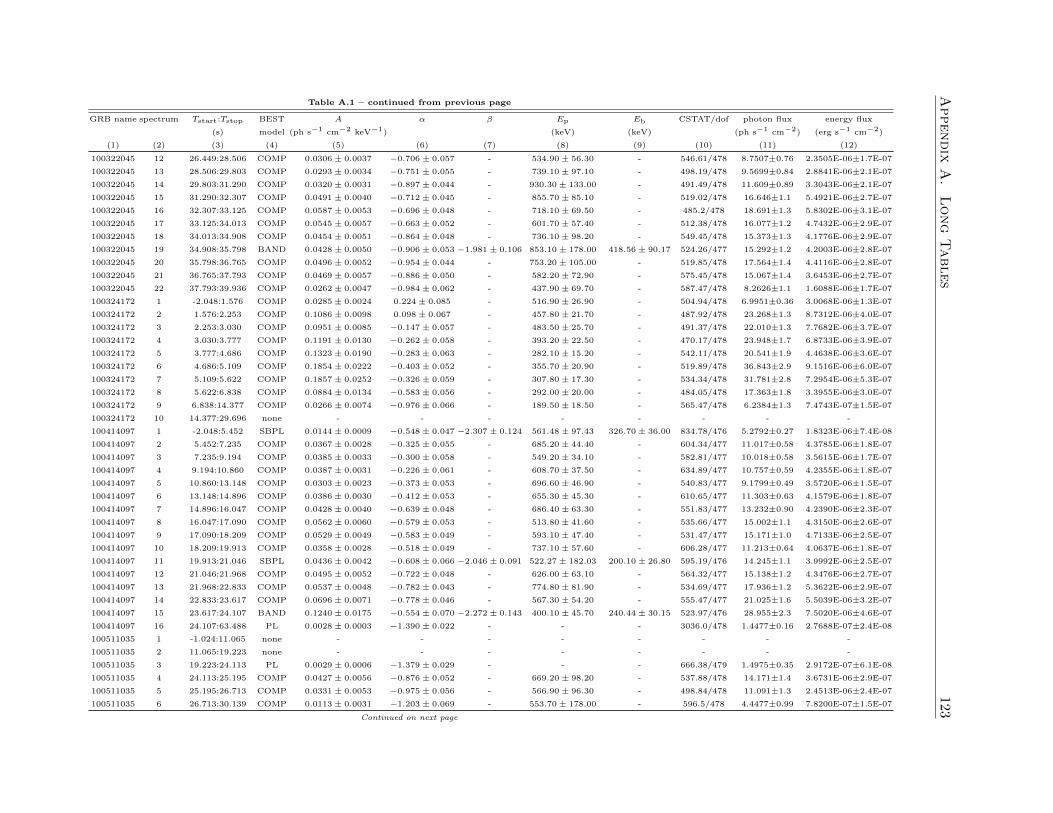
Appendix
A.
Long
Tables
123Table A.1 – continued from previous page
GRB name spectrum Tstart:Tstop BEST A α β Ep Eb CSTAT/dof photon flux energy flux
(s) model (ph s−1 cm−2 keV−1) (keV) (keV) (ph s−1 cm−2) (erg s−1 cm−2)
(1) (2) (3) (4) (5) (6) (7) (8) (9) (10) (11) (12)
100322045 12 26.449:28.506 COMP 0.0306± 0.0037 −0.706± 0.057 - 534.90± 56.30 - 546.61/478 8.7507±0.76 2.3505E-06±1.7E-07
100322045 13 28.506:29.803 COMP 0.0293± 0.0034 −0.751± 0.055 - 739.10± 97.10 - 498.19/478 9.5699±0.84 2.8841E-06±2.1E-07
100322045 14 29.803:31.290 COMP 0.0320± 0.0031 −0.897± 0.044 - 930.30± 133.00 - 491.49/478 11.609±0.89 3.3043E-06±2.1E-07
100322045 15 31.290:32.307 COMP 0.0491± 0.0040 −0.712± 0.045 - 855.70± 85.10 - 519.02/478 16.646±1.1 5.4921E-06±2.7E-07
100322045 16 32.307:33.125 COMP 0.0587± 0.0053 −0.696± 0.048 - 718.10± 69.50 - 485.2/478 18.691±1.3 5.8302E-06±3.1E-07
100322045 17 33.125:34.013 COMP 0.0545± 0.0057 −0.663± 0.052 - 601.70± 57.40 - 512.38/478 16.077±1.2 4.7432E-06±2.9E-07
100322045 18 34.013:34.908 COMP 0.0454± 0.0051 −0.864± 0.048 - 736.10± 98.20 - 549.45/478 15.373±1.3 4.1776E-06±2.9E-07
100322045 19 34.908:35.798 BAND 0.0428± 0.0050 −0.906± 0.053 −1.981± 0.106 853.10± 178.00 418.56± 90.17 524.26/477 15.292±1.2 4.2003E-06±2.8E-07
100322045 20 35.798:36.765 COMP 0.0496± 0.0052 −0.954± 0.044 - 753.20± 105.00 - 519.85/478 17.564±1.4 4.4116E-06±2.8E-07
100322045 21 36.765:37.793 COMP 0.0469± 0.0057 −0.886± 0.050 - 582.20± 72.90 - 575.45/478 15.067±1.4 3.6453E-06±2.7E-07
100322045 22 37.793:39.936 COMP 0.0262± 0.0047 −0.984± 0.062 - 437.90± 69.70 - 587.47/478 8.2626±1.1 1.6088E-06±1.7E-07
100324172 1 -2.048:1.576 COMP 0.0285± 0.0024 0.224± 0.085 - 516.90± 26.90 - 504.94/478 6.9951±0.36 3.0068E-06±1.3E-07
100324172 2 1.576:2.253 COMP 0.1086± 0.0098 0.098± 0.067 - 457.80± 21.70 - 487.92/478 23.268±1.3 8.7312E-06±4.0E-07
100324172 3 2.253:3.030 COMP 0.0951± 0.0085 −0.147± 0.057 - 483.50± 25.70 - 491.37/478 22.010±1.3 7.7682E-06±3.7E-07
100324172 4 3.030:3.777 COMP 0.1191± 0.0130 −0.262± 0.058 - 393.20± 22.50 - 470.17/478 23.948±1.7 6.8733E-06±3.9E-07
100324172 5 3.777:4.686 COMP 0.1323± 0.0190 −0.283± 0.063 - 282.10± 15.20 - 542.11/478 20.541±1.9 4.4638E-06±3.6E-07
100324172 6 4.686:5.109 COMP 0.1854± 0.0222 −0.403± 0.052 - 355.70± 20.90 - 519.89/478 36.843±2.9 9.1516E-06±6.0E-07
100324172 7 5.109:5.622 COMP 0.1857± 0.0252 −0.326± 0.059 - 307.80± 17.30 - 534.34/478 31.781±2.8 7.2954E-06±5.3E-07
100324172 8 5.622:6.838 COMP 0.0884± 0.0134 −0.583± 0.056 - 292.00± 20.00 - 484.05/478 17.363±1.8 3.3955E-06±3.0E-07
100324172 9 6.838:14.377 COMP 0.0266± 0.0074 −0.976± 0.066 - 189.50± 18.50 - 565.47/478 6.2384±1.3 7.4743E-07±1.5E-07
100324172 10 14.377:29.696 none - - - - - - - -
100414097 1 -2.048:5.452 SBPL 0.0144± 0.0009 −0.548± 0.047 −2.307± 0.124 561.48± 97.43 326.70± 36.00 834.78/476 5.2792±0.27 1.8323E-06±7.4E-08
100414097 2 5.452:7.235 COMP 0.0367± 0.0028 −0.325± 0.055 - 685.20± 44.40 - 604.34/477 11.017±0.58 4.3785E-06±1.8E-07
100414097 3 7.235:9.194 COMP 0.0385± 0.0033 −0.300± 0.058 - 549.20± 34.10 - 582.81/477 10.018±0.58 3.5615E-06±1.7E-07
100414097 4 9.194:10.860 COMP 0.0387± 0.0031 −0.226± 0.061 - 608.70± 37.50 - 634.89/477 10.757±0.59 4.2355E-06±1.8E-07
100414097 5 10.860:13.148 COMP 0.0303± 0.0023 −0.373± 0.053 - 696.60± 46.90 - 540.83/477 9.1799±0.49 3.5720E-06±1.5E-07
100414097 6 13.148:14.896 COMP 0.0386± 0.0030 −0.412± 0.053 - 655.30± 45.30 - 610.65/477 11.303±0.63 4.1579E-06±1.8E-07
100414097 7 14.896:16.047 COMP 0.0428± 0.0040 −0.639± 0.048 - 686.40± 63.30 - 551.83/477 13.232±0.90 4.2390E-06±2.3E-07
100414097 8 16.047:17.090 COMP 0.0562± 0.0060 −0.579± 0.053 - 513.80± 41.60 - 535.66/477 15.002±1.1 4.3150E-06±2.6E-07
100414097 9 17.090:18.209 COMP 0.0529± 0.0049 −0.583± 0.049 - 593.10± 47.40 - 531.47/477 15.171±1.0 4.7133E-06±2.5E-07
100414097 10 18.209:19.913 COMP 0.0358± 0.0028 −0.518± 0.049 - 737.10± 57.60 - 606.28/477 11.213±0.64 4.0637E-06±1.8E-07
100414097 11 19.913:21.046 SBPL 0.0436± 0.0042 −0.608± 0.066 −2.046± 0.091 522.27± 182.03 200.10± 26.80 595.19/476 14.245±1.1 3.9992E-06±2.5E-07
100414097 12 21.046:21.968 COMP 0.0495± 0.0052 −0.722± 0.048 - 626.00± 63.10 - 564.32/477 15.138±1.2 4.3476E-06±2.7E-07
100414097 13 21.968:22.833 COMP 0.0537± 0.0048 −0.782± 0.043 - 774.80± 81.90 - 534.69/477 17.936±1.2 5.3622E-06±2.9E-07
100414097 14 22.833:23.617 COMP 0.0696± 0.0071 −0.778± 0.046 - 567.30± 54.20 - 555.47/477 21.025±1.6 5.5039E-06±3.2E-07
100414097 15 23.617:24.107 BAND 0.1240± 0.0175 −0.554± 0.070 −2.272± 0.143 400.10± 45.70 240.44± 30.15 523.97/476 28.955±2.3 7.5020E-06±4.6E-07
100414097 16 24.107:63.488 PL 0.0028± 0.0003 −1.390± 0.022 - - - 3036.0/478 1.4477±0.16 2.7688E-07±2.4E-08
100511035 1 -1.024:11.065 none - - - - - - - -
100511035 2 11.065:19.223 none - - - - - - - -
100511035 3 19.223:24.113 PL 0.0029± 0.0006 −1.379± 0.029 - - - 666.38/479 1.4975±0.35 2.9172E-07±6.1E-08
100511035 4 24.113:25.195 COMP 0.0427± 0.0056 −0.876± 0.052 - 669.20± 98.20 - 537.88/478 14.171±1.4 3.6731E-06±2.9E-07
100511035 5 25.195:26.713 COMP 0.0331± 0.0053 −0.975± 0.056 - 566.90± 96.30 - 498.84/478 11.091±1.3 2.4513E-06±2.4E-07
100511035 6 26.713:30.139 COMP 0.0113± 0.0031 −1.203± 0.069 - 553.70± 178.00 - 596.5/478 4.4477±0.99 7.8200E-07±1.5E-07
Continued on next page
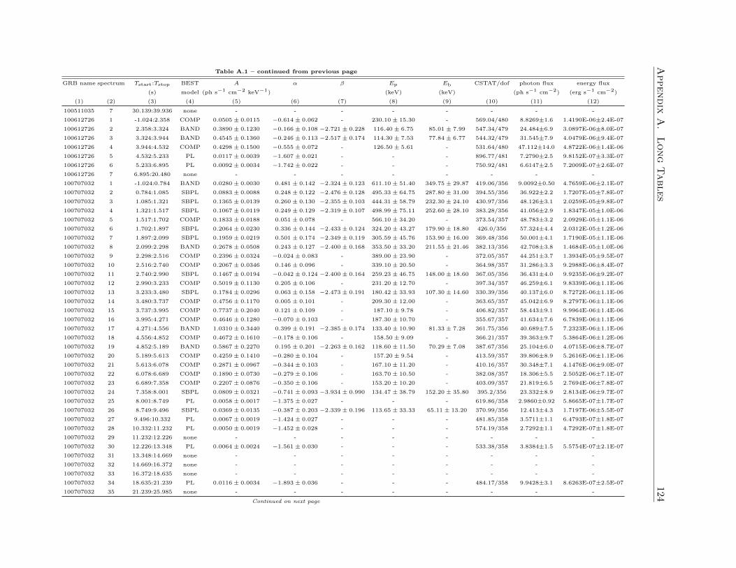
Appendix
A.
Long
Tables
124Table A.1 – continued from previous page
GRB name spectrum Tstart:Tstop BEST A α β Ep Eb CSTAT/dof photon flux energy flux
(s) model (ph s−1 cm−2 keV−1) (keV) (keV) (ph s−1 cm−2) (erg s−1 cm−2)
(1) (2) (3) (4) (5) (6) (7) (8) (9) (10) (11) (12)
100511035 7 30.139:39.936 none - - - - - - - -
100612726 1 -1.024:2.358 COMP 0.0505± 0.0115 −0.614± 0.062 - 230.10± 15.30 - 569.04/480 8.8269±1.6 1.4190E-06±2.4E-07
100612726 2 2.358:3.324 BAND 0.3890± 0.1230 −0.166± 0.108 −2.721± 0.228 116.40± 6.75 85.01± 7.99 547.34/479 24.484±6.9 3.0897E-06±8.0E-07
100612726 3 3.324:3.944 BAND 0.4545± 0.1360 −0.246± 0.113 −2.517± 0.174 114.30± 7.53 77.84± 6.77 544.32/479 31.545±7.9 4.0479E-06±9.4E-07
100612726 4 3.944:4.532 COMP 0.4298± 0.1500 −0.555± 0.072 - 126.50± 5.61 - 531.64/480 47.112±14.0 4.8722E-06±1.4E-06
100612726 5 4.532:5.233 PL 0.0117± 0.0039 −1.607± 0.021 - - - 896.77/481 7.2790±2.5 9.8152E-07±3.3E-07
100612726 6 5.233:6.895 PL 0.0092± 0.0034 −1.742± 0.022 - - - 750.92/481 6.6147±2.5 7.2009E-07±2.6E-07
100612726 7 6.895:20.480 none - - - - - - - -
100707032 1 -1.024:0.784 BAND 0.0280± 0.0030 0.481± 0.142 −2.324± 0.123 611.10± 51.40 349.75± 29.87 419.06/356 9.0092±0.50 4.7659E-06±2.1E-07
100707032 2 0.784:1.085 SBPL 0.0883± 0.0088 0.248± 0.122 −2.476± 0.128 495.33± 64.75 287.80± 31.00 394.55/356 36.922±2.2 1.7207E-05±7.8E-07
100707032 3 1.085:1.321 SBPL 0.1365± 0.0139 0.260± 0.130 −2.355± 0.103 444.31± 58.79 232.30± 24.10 430.97/356 48.126±3.1 2.0259E-05±9.8E-07
100707032 4 1.321:1.517 SBPL 0.1067± 0.0119 0.249± 0.129 −2.319± 0.107 498.99± 75.11 252.60± 28.10 383.28/356 41.056±2.9 1.8347E-05±1.0E-06
100707032 5 1.517:1.702 COMP 0.1833± 0.0188 0.051± 0.078 - 566.10± 34.20 - 373.54/357 48.783±3.2 2.0929E-05±1.1E-06
100707032 6 1.702:1.897 SBPL 0.2064± 0.0230 0.336± 0.144 −2.433± 0.124 324.20± 43.27 179.90± 18.80 426.0/356 57.324±4.4 2.0312E-05±1.2E-06
100707032 7 1.897:2.099 SBPL 0.1959± 0.0219 0.501± 0.174 −2.349± 0.119 305.59± 45.76 153.90± 16.00 369.48/356 50.001±4.1 1.7190E-05±1.1E-06
100707032 8 2.099:2.298 BAND 0.2678± 0.0508 0.243± 0.127 −2.400± 0.168 353.50± 33.20 211.55± 21.46 382.13/356 42.708±3.8 1.4684E-05±1.0E-06
100707032 9 2.298:2.516 COMP 0.2396± 0.0324 −0.024± 0.083 - 389.00± 23.90 - 372.05/357 44.251±3.7 1.3934E-05±9.5E-07
100707032 10 2.516:2.740 COMP 0.2067± 0.0346 0.146± 0.096 - 339.10± 20.50 - 364.98/357 31.286±3.3 9.2988E-06±8.4E-07
100707032 11 2.740:2.990 SBPL 0.1467± 0.0194 −0.042± 0.124 −2.400± 0.164 259.23± 46.75 148.00± 18.60 367.05/356 36.431±4.0 9.9235E-06±9.2E-07
100707032 12 2.990:3.233 COMP 0.5019± 0.1130 0.205± 0.106 - 231.20± 12.70 - 397.34/357 46.259±6.1 9.8339E-06±1.1E-06
100707032 13 3.233:3.480 SBPL 0.1784± 0.0296 0.063± 0.158 −2.473± 0.191 180.42± 33.93 107.30± 14.60 330.39/356 40.137±6.0 8.7272E-06±1.1E-06
100707032 14 3.480:3.737 COMP 0.4756± 0.1170 0.005± 0.101 - 209.30± 12.00 - 363.65/357 45.042±6.9 8.2797E-06±1.1E-06
100707032 15 3.737:3.995 COMP 0.7737± 0.2040 0.121± 0.109 - 187.10± 9.78 - 406.82/357 58.443±9.1 9.9964E-06±1.4E-06
100707032 16 3.995:4.271 COMP 0.4646± 0.1280 −0.070± 0.103 - 187.30± 10.70 - 355.67/357 41.634±7.6 6.7839E-06±1.1E-06
100707032 17 4.271:4.556 BAND 1.0310± 0.3440 0.399± 0.191 −2.385± 0.174 133.40± 10.90 81.33± 7.28 361.75/356 40.689±7.5 7.2323E-06±1.1E-06
100707032 18 4.556:4.852 COMP 0.4672± 0.1610 −0.178± 0.106 - 158.50± 9.09 - 366.21/357 39.363±9.7 5.3864E-06±1.2E-06
100707032 19 4.852:5.189 BAND 0.5867± 0.2270 0.195± 0.201 −2.263± 0.162 118.60± 11.50 70.29± 7.08 387.67/356 25.104±6.0 4.0715E-06±8.7E-07
100707032 20 5.189:5.613 COMP 0.4259± 0.1410 −0.280± 0.104 - 157.20± 9.54 - 413.59/357 39.806±8.9 5.2616E-06±1.1E-06
100707032 21 5.613:6.078 COMP 0.2871± 0.0967 −0.344± 0.103 - 167.10± 11.20 - 410.16/357 30.348±7.1 4.1476E-06±9.0E-07
100707032 22 6.078:6.689 COMP 0.1890± 0.0730 −0.279± 0.106 - 163.70± 10.50 - 382.08/357 18.306±5.5 2.5052E-06±7.1E-07
100707032 23 6.689:7.358 COMP 0.2207± 0.0876 −0.350± 0.106 - 153.20± 10.20 - 403.09/357 21.819±6.5 2.7694E-06±7.8E-07
100707032 24 7.358:8.001 SBPL 0.0809± 0.0321 −0.741± 0.093 −3.934± 0.990 134.47± 38.79 152.20± 35.80 395.2/356 23.332±8.9 2.8134E-06±9.7E-07
100707032 25 8.001:8.749 PL 0.0058± 0.0017 −1.375± 0.027 - - - 619.86/358 2.9860±0.92 5.8665E-07±1.7E-07
100707032 26 8.749:9.496 SBPL 0.0369± 0.0135 −0.387± 0.203 −2.339± 0.196 113.65± 33.33 65.11± 13.20 370.99/356 12.413±4.3 1.7197E-06±5.5E-07
100707032 27 9.496:10.332 PL 0.0067± 0.0019 −1.424± 0.027 - - - 481.85/358 3.5711±1.1 6.4793E-07±1.8E-07
100707032 28 10.332:11.232 PL 0.0050± 0.0019 −1.452± 0.028 - - - 574.19/358 2.7292±1.1 4.7292E-07±1.8E-07
100707032 29 11.232:12.226 none - - - - - - - -
100707032 30 12.226:13.348 PL 0.0064± 0.0024 −1.561± 0.030 - - - 533.38/358 3.8384±1.5 5.5754E-07±2.1E-07
100707032 31 13.348:14.669 none - - - - - - - -
100707032 32 14.669:16.372 none - - - - - - - -
100707032 33 16.372:18.635 none - - - - - - - -
100707032 34 18.635:21.239 PL 0.0116± 0.0034 −1.893± 0.036 - - - 484.17/358 9.9428±3.1 8.6263E-07±2.5E-07
100707032 35 21.239:25.985 none - - - - - - - -
Continued on next page
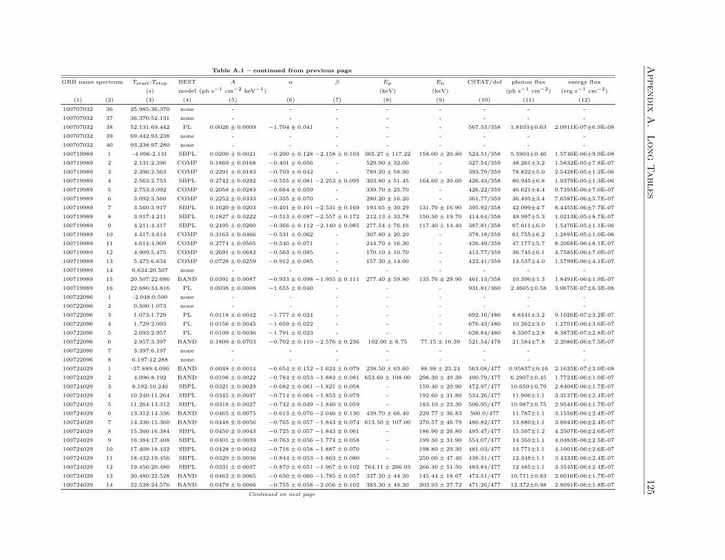
Appendix
A.
Long
Tables
125Table A.1 – continued from previous page
GRB name spectrum Tstart:Tstop BEST A α β Ep Eb CSTAT/dof photon flux energy flux
(s) model (ph s−1 cm−2 keV−1) (keV) (keV) (ph s−1 cm−2) (erg s−1 cm−2)
(1) (2) (3) (4) (5) (6) (7) (8) (9) (10) (11) (12)
100707032 36 25.985:36.370 none - - - - - - - -
100707032 37 36.370:52.131 none - - - - - - - -
100707032 38 52.131:69.442 PL 0.0026± 0.0009 −1.704± 0.041 - - - 567.53/358 1.8103±0.63 2.0911E-07±6.9E-08
100707032 39 69.442:93.238 none - - - - - - - -
100707032 40 93.238:97.280 none - - - - - - - -
100719989 1 -4.096:2.131 SBPL 0.0200± 0.0021 −0.290± 0.128 −2.158± 0.103 365.27± 117.22 158.00± 20.80 524.51/358 5.5903±0.46 1.5746E-06±9.9E-08
100719989 2 2.131:2.396 COMP 0.1869± 0.0168 −0.401± 0.056 - 529.90± 32.00 - 327.54/359 48.261±3.2 1.5832E-05±7.8E-07
100719989 3 2.396:2.563 COMP 0.2391± 0.0183 −0.703± 0.042 - 789.20± 58.90 - 393.79/359 78.822±5.0 2.5428E-05±1.2E-06
100719989 4 2.563:2.753 SBPL 0.2742± 0.0292 −0.555± 0.081 −2.253± 0.095 303.80± 51.45 164.60± 20.60 426.43/358 80.945±6.8 1.9379E-05±1.3E-06
100719989 5 2.753:3.092 COMP 0.2058± 0.0283 −0.664± 0.059 - 339.70± 25.70 - 426.22/359 46.621±4.4 9.7395E-06±7.0E-07
100719989 6 3.092:3.560 COMP 0.2252± 0.0333 −0.355± 0.070 - 280.20± 16.20 - 361.77/359 36.495±3.4 7.6587E-06±5.7E-07
100719989 7 3.560:3.917 SBPL 0.1620± 0.0203 −0.401± 0.101 −2.531± 0.169 193.65± 30.29 131.70± 16.90 395.92/358 42.099±4.7 8.4455E-06±7.7E-07
100719989 8 3.917:4.211 SBPL 0.1827± 0.0222 −0.513± 0.087 −2.557± 0.172 212.13± 33.78 150.30± 19.70 414.64/358 49.997±5.3 1.0213E-05±8.7E-07
100719989 9 4.211:4.417 SBPL 0.2495± 0.0260 −0.366± 0.112 −2.140± 0.085 277.54± 76.16 117.40± 14.40 387.81/358 67.611±6.0 1.5476E-05±1.1E-06
100719989 10 4.417:4.614 COMP 0.3163± 0.0466 −0.531± 0.062 - 307.80± 20.20 - 378.18/359 61.755±6.2 1.2895E-05±1.0E-06
100719989 11 4.614:4.909 COMP 0.2774± 0.0505 −0.540± 0.071 - 244.70± 16.30 - 436.49/359 47.177±5.7 8.2068E-06±8.1E-07
100719989 12 4.909:5.475 COMP 0.2691± 0.0682 −0.563± 0.085 - 170.10± 10.70 - 413.77/359 36.745±6.1 4.7585E-06±7.0E-07
100719989 13 5.475:6.634 COMP 0.0728± 0.0259 −0.912± 0.085 - 157.30± 14.00 - 423.41/359 14.537±4.0 1.5799E-06±4.1E-07
100719989 14 6.634:20.507 none - - - - - - - -
100719989 15 20.507:22.686 BAND 0.0391± 0.0087 −0.933± 0.098 −1.955± 0.111 277.40± 59.80 135.76± 29.90 461.13/358 10.396±1.3 1.8491E-06±1.9E-07
100719989 16 22.686:34.816 PL 0.0038± 0.0008 −1.655± 0.040 - - - 931.81/360 2.4605±0.58 3.0675E-07±6.3E-08
100722096 1 -2.048:0.500 none - - - - - - - -
100722096 2 0.500:1.073 none - - - - - - - -
100722096 3 1.073:1.729 PL 0.0118± 0.0042 −1.777± 0.024 - - - 692.16/480 8.8441±3.2 9.1026E-07±3.2E-07
100722096 4 1.729:2.093 PL 0.0156± 0.0045 −1.659± 0.022 - - - 676.43/480 10.262±3.0 1.2701E-06±3.6E-07
100722096 5 2.093:2.957 PL 0.0109± 0.0036 −1.791± 0.023 - - - 628.84/480 8.3307±2.8 8.3873E-07±2.8E-07
100722096 6 2.957:3.397 BAND 0.1809± 0.0703 −0.702± 0.110 −2.576± 0.236 102.00± 8.75 77.15± 10.39 521.54/478 21.584±7.8 2.2086E-06±7.5E-07
100722096 7 3.397:6.197 none - - - - - - - -
100722096 8 6.197:12.288 none - - - - - - - -
100724029 1 -37.889:4.096 BAND 0.0048± 0.0014 −0.654± 0.152 −1.624± 0.079 238.50± 63.60 88.98± 23.24 563.08/477 0.95837±0.16 2.1635E-07±3.0E-08
100724029 2 4.096:8.192 BAND 0.0198± 0.0022 −0.784± 0.053 −1.883± 0.081 653.60± 108.00 298.30± 49.39 490.79/477 6.2907±0.45 1.7724E-06±1.0E-07
100724029 3 8.192:10.240 SBPL 0.0321± 0.0029 −0.682± 0.061 −1.821± 0.058 - 159.40± 20.90 472.97/477 10.659±0.79 2.8408E-06±1.7E-07
100724029 4 10.240:11.264 SBPL 0.0345± 0.0037 −0.714± 0.064 −1.853± 0.079 - 192.60± 31.80 534.26/477 11.906±1.1 3.3137E-06±2.4E-07
100724029 5 11.264:13.312 SBPL 0.0318± 0.0027 −0.742± 0.049 −1.840± 0.059 - 183.10± 23.30 506.95/477 10.987±0.75 2.9541E-06±1.7E-07
100724029 6 13.312:14.336 BAND 0.0465± 0.0075 −0.613± 0.076 −2.046± 0.130 439.70± 66.40 229.77± 36.83 500.0/477 11.787±1.1 3.1556E-06±2.4E-07
100724029 7 14.336:15.360 BAND 0.0448± 0.0056 −0.765± 0.057 −1.843± 0.074 613.50± 107.00 270.57± 46.79 480.82/477 13.880±1.1 3.8943E-06±2.4E-07
100724029 8 15.360:16.384 SBPL 0.0450± 0.0043 −0.725± 0.057 −1.843± 0.061 - 186.90± 26.80 495.47/477 15.507±1.2 4.2507E-06±2.6E-07
100724029 9 16.384:17.408 SBPL 0.0401± 0.0039 −0.763± 0.056 −1.774± 0.058 - 199.30± 31.90 554.07/477 14.350±1.1 4.0483E-06±2.5E-07
100724029 10 17.408:18.432 SBPL 0.0428± 0.0042 −0.716± 0.058 −1.887± 0.070 - 198.80± 29.30 481.03/477 14.771±1.1 4.1001E-06±2.6E-07
100724029 11 18.432:19.456 SBPL 0.0329± 0.0036 −0.844± 0.053 −1.863± 0.080 - 250.00± 47.40 438.31/477 12.348±1.1 3.4333E-06±2.4E-07
100724029 12 19.456:20.480 SBPL 0.0331± 0.0037 −0.870± 0.051 −1.967± 0.102 764.11± 266.93 266.40± 51.50 483.84/477 12.485±1.1 3.3545E-06±2.4E-07
100724029 13 20.480:22.528 BAND 0.0462± 0.0065 −0.650± 0.066 −1.785± 0.057 337.20± 44.20 145.44± 18.67 473.51/477 10.711±0.83 2.6016E-06±1.7E-07
100724029 14 22.528:24.576 BAND 0.0479± 0.0066 −0.755± 0.058 −2.056± 0.102 383.30± 49.30 203.93± 27.72 471.26/477 12.372±0.98 2.8091E-06±1.8E-07
Continued on next page
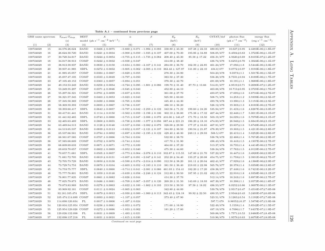
Appendix
A.
Long
Tables
126Table A.1 – continued from previous page
GRB name spectrum Tstart:Tstop BEST A α β Ep Eb CSTAT/dof photon flux energy flux
(s) model (ph s−1 cm−2 keV−1) (keV) (keV) (ph s−1 cm−2) (erg s−1 cm−2)
(1) (2) (3) (4) (5) (6) (7) (8) (9) (10) (11) (12)
100724029 15 24.576:26.624 BAND 0.0466± 0.0075 −0.660± 0.071 −1.984± 0.093 330.80± 43.30 167.28± 22.33 480.83/477 10.627±0.95 2.4293E-06±1.8E-07
100724029 16 26.624:30.720 BAND 0.0221± 0.0034 −0.900± 0.059 −1.935± 0.107 407.00± 70.30 193.86± 34.88 506.05/477 6.4584±0.63 1.3723E-06±1.1E-07
100724029 17 30.720:34.817 BAND 0.0224± 0.0054 −0.755± 0.115 −1.735± 0.084 208.40± 43.30 85.58± 17.22 456.31/477 4.5620±0.69 8.8105E-07±1.2E-07
100724029 18 34.817:38.913 COMP 0.0222± 0.0032 −0.938± 0.047 - 414.00± 48.40 - 436.74/478 6.6253±0.70 1.3022E-06±1.1E-07
100724029 19 38.913:39.937 BAND 0.0830± 0.0158 −0.634± 0.083 −2.167± 0.141 284.00± 36.70 162.39± 22.85 461.24/477 17.056±1.8 3.5444E-06±3.0E-07
100724029 20 39.937:41.985 SBPL 0.0272± 0.0032 −0.805± 0.062 −2.005± 0.110 362.42± 127.97 141.00± 22.10 434.0/477 9.0772±0.97 1.9193E-06±1.8E-07
100724029 21 41.985:45.057 COMP 0.0384± 0.0067 −0.829± 0.055 - 278.30± 24.90 - 504.23/478 9.0373±1.1 1.5017E-06±1.5E-07
100724029 22 45.057:47.105 COMP 0.0333± 0.0049 −0.797± 0.050 - 383.50± 37.30 - 556.26/478 8.7331±0.94 1.8189E-06±1.7E-07
100724029 23 47.105:49.153 COMP 0.0363± 0.0057 −0.894± 0.051 - 378.30± 42.70 - 491.69/478 10.191±1.1 1.9689E-06±1.8E-07
100724029 24 49.153:53.249 BAND 0.0258± 0.0054 −0.724± 0.095 −1.801± 0.086 199.70± 31.40 87.73± 13.66 514.81/477 4.9519±0.71 9.2690E-07±1.2E-07
100724029 25 53.249:55.297 COMP 0.0371± 0.0046 −0.845± 0.043 - 452.80± 44.10 - 463.06/478 10.713±0.95 2.3725E-06±1.7E-07
100724029 26 55.297:56.321 COMP 0.0761± 0.0099 −0.657± 0.051 - 361.00± 27.70 - 493.07/478 17.695±1.6 3.8716E-06±2.7E-07
100724029 27 56.321:57.345 COMP 0.0463± 0.0053 −0.823± 0.043 - 565.90± 60.60 - 506.71/478 14.253±1.2 3.5939E-06±2.5E-07
100724029 28 57.345:58.369 COMP 0.0490± 0.0066 −0.765± 0.050 - 445.40± 44.30 - 493.78/478 13.390±1.3 3.1155E-06±2.5E-07
100724029 29 58.369:59.393 COMP 0.0693± 0.0067 −0.736± 0.037 - 486.10± 36.20 - 526.12/478 19.303±1.3 4.8185E-06±2.7E-07
100724029 30 59.393:60.417 SBPL 0.0642± 0.0057 −0.797± 0.042 −2.259± 0.122 342.56± 71.22 199.60± 24.20 535.94/477 21.423±1.6 4.8267E-06±3.0E-07
100724029 31 60.417:61.441 BAND 0.1114± 0.0150 −0.562± 0.059 −2.198± 0.106 302.10± 26.80 175.38± 17.32 467.44/477 22.448±1.7 5.0011E-06±3.1E-07
100724029 32 61.441:62.465 SBPL 0.0743± 0.0060 −0.715± 0.047 −2.088± 0.078 416.06± 140.47 171.70± 18.50 503.19/477 24.029±1.6 5.7076E-06±3.1E-07
100724029 33 62.465:63.489 SBPL 0.0800± 0.0055 −0.738± 0.039 −1.977± 0.056 687.44± 221.21 186.20± 18.10 474.83/477 26.948±1.5 6.8841E-06±3.1E-07
100724029 34 63.489:64.513 BAND 0.1128± 0.0140 −0.557± 0.056 −2.082± 0.079 328.00± 29.90 177.27± 16.65 467.91/477 23.837±1.6 5.6749E-06±3.1E-07
100724029 35 64.513:65.537 BAND 0.0839± 0.0113 −0.652± 0.057 −2.121± 0.107 344.80± 36.50 190.94± 21.87 478.39/477 19.303±1.5 4.4211E-06±2.8E-07
100724029 36 65.537:66.561 BAND 0.0784± 0.0092 −0.697± 0.050 −2.195± 0.122 429.40± 46.30 249.11± 29.93 508.5/477 20.415±1.4 5.0252E-06±2.8E-07
100724029 37 66.561:67.585 COMP 0.0767± 0.0066 −0.764± 0.034 - 532.90± 38.70 - 538.78/478 22.468±1.4 5.7674E-06±2.9E-07
100724029 38 67.585:68.609 COMP 0.0702± 0.0078 −0.744± 0.041 - 417.70± 31.90 - 496.43/478 18.443±1.5 4.1937E-06±2.7E-07
100724029 39 68.609:69.633 COMP 0.0671± 0.0071 −0.772± 0.039 - 464.60± 37.20 - 513.37/478 18.735±1.4 4.4414E-06±2.7E-07
100724029 40 69.633:70.657 COMP 0.0602± 0.0069 −0.852± 0.040 - 475.30± 44.60 - 538.34/478 17.762±1.5 4.0123E-06±2.7E-07
100724029 41 70.657:71.681 SBPL 0.0505± 0.0057 −0.773± 0.064 −2.078± 0.110 332.87± 115.55 147.00± 21.70 537.22/477 16.447±1.6 3.4920E-06±2.9E-07
100724029 42 71.681:72.705 BAND 0.0619± 0.0131 −0.607± 0.091 −2.047± 0.141 252.20± 34.40 133.27± 20.08 454.75/477 11.759±1.5 2.3931E-06±2.7E-07
100724029 43 72.705:73.729 BAND 0.0850± 0.0138 −0.590± 0.074 −2.014± 0.090 312.50± 38.20 161.11± 20.04 462.41/477 17.929±1.6 4.1366E-06±2.9E-07
100724029 44 73.729:74.753 BAND 0.0870± 0.0104 −0.603± 0.052 −2.183± 0.110 381.50± 36.40 219.03± 22.98 565.76/477 20.378±1.4 5.0358E-06±2.8E-07
100724029 45 74.753:75.777 SBPL 0.0840± 0.0060 −0.714± 0.041 −2.081± 0.066 461.03± 154.41 182.20± 17.20 458.38/477 27.448±1.6 6.7421E-06±3.2E-07
100724029 46 75.777:76.801 BAND 0.1059± 0.0148 −0.639± 0.058 −2.246± 0.124 312.80± 30.50 187.95± 21.02 482.15/477 22.910±1.8 4.9358E-06±3.1E-07
100724029 47 76.801:77.825 COMP 0.0661± 0.0082 −0.826± 0.044 - 414.30± 37.70 - 512.14/478 18.243±1.6 3.8973E-06±2.7E-07
100724029 48 77.825:79.873 BAND 0.0486± 0.0081 −0.709± 0.067 −2.057± 0.120 269.20± 31.50 143.69± 18.93 467.39/477 10.398±1.1 2.0572E-06±1.8E-07
100724029 49 79.873:83.969 BAND 0.0278± 0.0063 −0.822± 0.100 −1.862± 0.103 213.50± 39.50 97.58± 18.02 496.53/477 6.0252±0.86 1.0697E-06±1.3E-07
100724029 50 83.969:92.161 COMP 0.0111± 0.0024 −0.865± 0.063 - 342.80± 44.00 - 539.78/478 2.9317±0.47 5.4516E-07±7.6E-08
100724029 51 92.161:105.474 SBPL 0.0079± 0.0013 −0.930± 0.089 −1.900± 0.113 342.43± 124.18 99.92± 22.50 490.55/477 2.9344±0.43 5.2493E-07±6.6E-08
100724029 52 105.474:114.690 COMP 0.0093± 0.0021 −1.107± 0.057 - 373.40± 67.90 - 523.51/478 3.1263±0.54 5.1192E-07±7.6E-08
100724029 53 114.690:120.834 PL 0.0017± 0.0006 −1.497± 0.024 - - - 597.7/479 0.98552±0.37 1.5879E-07±5.9E-08
100724029 54 120.834:125.954 COMP 0.0236± 0.0081 −0.953± 0.072 - 171.60± 16.90 - 522.49/478 5.1559±1.4 5.8542E-07±1.5E-07
100724029 55 125.954:129.026 COMP 0.0272± 0.0086 −1.033± 0.062 - 181.20± 17.80 - 497.19/478 6.7096±1.7 7.6437E-07±1.9E-07
100724029 56 129.026:132.098 PL 0.0031± 0.0009 −1.493± 0.021 - - - 569.88/479 1.7571±0.53 2.8480E-07±8.4E-08
100724029 57 132.098:137.218 PL 0.0031± 0.0010 −1.615± 0.030 - - - 510.96/479 1.9579±0.63 2.6070E-07±8.0E-08
Continued on next page
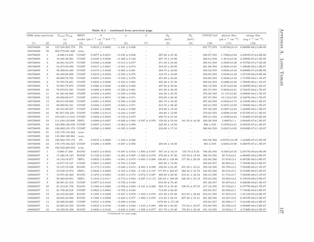
Appendix
A.
Long
Tables
127Table A.1 – continued from previous page
GRB name spectrum Tstart:Tstop BEST A α β Ep Eb CSTAT/dof photon flux energy flux
(s) model (ph s−1 cm−2 keV−1) (keV) (keV) (ph s−1 cm−2) (erg s−1 cm−2)
(1) (2) (3) (4) (5) (6) (7) (8) (9) (10) (11) (12)
100724029 58 137.218:203.779 PL 0.0010± 0.0002 −1.541± 0.028 - - - 627.77/479 0.58728±0.14 8.8066E-08±2.0E-08
100724029 59 203.779:231.428 none - - - - - - - -
100728095 1 -4.096:19.456 COMP 0.0077± 0.0015 −0.556± 0.092 - 387.20± 47.30 - 392.87/359 1.7386±0.22 4.2381E-07±4.2E-08
100728095 2 19.456:46.081 COMP 0.0109± 0.0039 −0.396± 0.122 - 207.70± 19.90 - 466.01/359 1.4514±0.36 2.3390E-07±5.3E-08
100728095 3 46.081:54.273 COMP 0.0166± 0.0028 −0.514± 0.077 - 371.30± 35.80 - 365.91/359 3.5939±0.38 8.7075E-07±7.5E-08
100728095 4 54.273:58.369 COMP 0.0317± 0.0051 −0.501± 0.074 - 344.00± 29.90 - 361.98/359 6.5000±0.65 1.4994E-06±1.2E-07
100728095 5 58.369:63.489 COMP 0.0176± 0.0032 −0.560± 0.081 - 384.70± 42.80 - 340.52/359 4.0030±0.48 9.6908E-07±9.6E-08
100728095 6 63.489:68.609 COMP 0.0210± 0.0032 −0.550± 0.075 - 416.70± 43.00 - 356.65/359 4.9538±0.49 1.2741E-06±9.8E-08
100728095 7 68.609:72.705 COMP 0.0255± 0.0034 −0.523± 0.070 - 451.90± 43.20 - 364.86/359 6.2348±0.54 1.7195E-06±1.1E-07
100728095 8 72.705:76.801 COMP 0.0233± 0.0028 −0.525± 0.065 - 505.20± 47.20 - 369.04/359 6.0486±0.48 1.7862E-06±1.1E-07
100728095 9 76.801:79.873 COMP 0.0380± 0.0046 −0.460± 0.062 - 407.00± 30.60 - 382.13/359 8.4714±0.66 2.2580E-06±1.4E-07
100728095 10 79.873:81.921 COMP 0.0408± 0.0050 −0.526± 0.061 - 451.90± 38.30 - 405.57/359 9.9638±0.81 2.7421E-06±1.7E-07
100728095 11 81.921:83.969 COMP 0.0459± 0.0053 −0.538± 0.058 - 443.30± 35.50 - 376.36/359 11.147±0.85 3.0089E-06±1.7E-07
100728095 12 83.969:86.017 COMP 0.0515± 0.0074 −0.390± 0.071 - 353.90± 26.40 - 337.97/359 10.112±0.90 2.5207E-06±1.7E-07
100728095 13 86.017:89.089 COMP 0.0381± 0.0050 −0.582± 0.058 - 391.70± 32.30 - 387.62/359 8.8332±0.75 2.1384E-06±1.4E-07
100728095 14 89.089:92.161 COMP 0.0403± 0.0070 −0.602± 0.071 - 312.70± 28.40 - 392.21/359 8.3321±0.92 1.7000E-06±1.5E-07
100728095 15 92.161:96.257 COMP 0.0405± 0.0082 −0.444± 0.080 - 254.80± 19.50 - 375.48/359 6.5287±0.84 1.2226E-06±1.3E-07
100728095 16 96.257:103.425 COMP 0.0380± 0.0114 −0.444± 0.097 - 184.80± 13.80 - 372.04/359 4.8398±0.98 6.9716E-07±1.3E-07
100728095 17 103.425:111.618 COMP 0.0204± 0.0045 −0.734± 0.075 - 266.70± 27.50 - 399.21/359 4.3198±0.64 7.3346E-07±9.2E-08
100728095 18 111.618:123.906 SBPL 0.0099± 0.0037 −0.848± 0.084 −3.567± 0.978 150.62± 53.94 161.50± 43.20 428.29/358 3.0687±1.1 3.9044E-07±1.2E-07
100728095 19 123.906:128.002 COMP 0.0407± 0.0101 −0.364± 0.090 - 222.90± 16.50 - 388.1/359 5.5476±0.91 9.5931E-07±1.4E-07
100728095 20 128.002:135.170 COMP 0.0360± 0.0085 −0.535± 0.083 - 216.60± 17.10 - 386.68/359 5.6247±0.85 8.9100E-07±1.1E-07
100728095 21 135.170:143.362 none - - - - - - - -
100728095 22 143.362:168.962 none - - - - - - - -
100728095 23 168.962:178.179 PL 0.0016± 0.0006 −1.543± 0.026 - - - 482.58/360 0.95701±0.38 1.4346E-07±5.5E-08
100728095 24 178.179:184.323 COMP 0.0290± 0.0090 −0.607± 0.093 - 200.00± 18.60 - 365.5/359 4.6204±0.98 6.6867E-07±1.3E-07
100728095 25 184.323:283.652 none - - - - - - - -
100826957 1 0.000:17.448 BAND 0.0457± 0.0032 −0.587± 0.034 −1.983± 0.037 307.10± 16.10 155.70± 8.25 786.28/356 9.5481±0.35 2.2017E-06±6.6E-08
100826957 2 17.448:18.143 BAND 0.1129± 0.0221 −0.481± 0.099 −1.929± 0.078 276.00± 37.20 135.58± 18.03 386.53/356 20.713±2.0 4.8688E-06±3.9E-07
100826957 3 18.143:18.677 SBPL 0.0835± 0.0094 −0.691± 0.070 −2.065± 0.096 430.66± 148.88 177.40± 26.50 442.96/356 27.019±2.4 6.6972E-06±4.8E-07
100826957 4 18.677:19.127 COMP 0.0847± 0.0093 −0.750± 0.048 - 665.00± 74.90 - 400.62/357 26.685±2.1 7.7003E-06±4.8E-07
100826957 5 19.127:19.558 BAND 0.1173± 0.0181 −0.628± 0.074 −2.063± 0.099 436.80± 64.40 231.39± 34.21 359.52/356 29.793±2.5 7.8530E-06±5.1E-07
100826957 6 19.558:19.975 SBPL 0.0848± 0.0092 −0.764± 0.056 −2.123± 0.107 577.95± 202.87 269.40± 45.70 345.56/356 30.516±2.5 8.5720E-06±5.4E-07
100826957 7 19.975:20.469 BAND 0.1270± 0.0203 −0.655± 0.074 −2.074± 0.097 408.60± 60.30 218.31± 32.54 349.41/356 31.716±2.7 7.9365E-06±5.1E-07
100826957 8 20.469:20.901 SBPL 0.1016± 0.0111 −0.712± 0.062 −2.207± 0.113 420.35± 106.09 220.40± 33.10 378.45/356 33.903±2.8 8.7391E-06±5.6E-07
100826957 9 20.901:21.312 COMP 0.0977± 0.0104 −0.739± 0.049 - 654.90± 70.40 - 391.26/357 30.487±2.4 8.8203E-06±5.3E-07
100826957 10 21.312:21.758 BAND 0.1569± 0.0266 −0.592± 0.082 −2.101± 0.098 363.70± 50.40 198.61± 27.55 417.12/356 35.732±3.1 8.7577E-06±5.7E-07
100826957 11 21.758:22.218 COMP 0.0823± 0.0085 −0.785± 0.046 - 714.60± 82.40 - 332.85/357 26.836±2.1 7.7484E-06±4.8E-07
100826957 12 22.218:22.605 BAND 0.1493± 0.0238 −0.597± 0.079 −1.959± 0.073 431.80± 67.00 213.55± 32.82 354.01/356 37.307±3.0 1.0111E-05±6.0E-07
100826957 13 22.605:23.088 BAND 0.1308± 0.0209 −0.622± 0.077 −1.990± 0.076 412.20± 62.10 207.26± 31.01 361.28/356 32.327±2.6 8.3947E-06±5.2E-07
100826957 14 23.088:23.685 COMP 0.0547± 0.0056 −0.939± 0.040 - 1070.00± 171.00 - 459.64/357 20.598±1.7 5.8416E-06±3.9E-07
100826957 15 23.685:24.359 BAND 0.0833± 0.0149 −0.680± 0.083 −1.910± 0.084 369.40± 62.00 175.04± 29.07 372.66/356 20.338±2.0 4.8928E-06±3.8E-07
100826957 16 24.359:25.236 BAND 0.0843± 0.0145 −0.639± 0.081 −1.928± 0.077 351.70± 53.40 170.23± 25.26 451.19/356 19.584±1.7 4.7196E-06±3.3E-07
Continued on next page
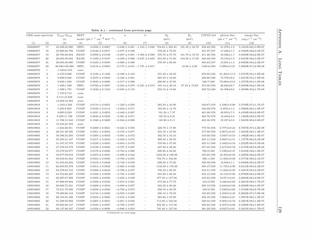
Appendix
A.
Long
Tables
128Table A.1 – continued from previous page
GRB name spectrum Tstart:Tstop BEST A α β Ep Eb CSTAT/dof photon flux energy flux
(s) model (ph s−1 cm−2 keV−1) (keV) (keV) (ph s−1 cm−2) (erg s−1 cm−2)
(1) (2) (3) (4) (5) (6) (7) (8) (9) (10) (11) (12)
100826957 17 25.236:25.890 SBPL 0.0592± 0.0067 −0.848± 0.061 −1.919± 0.082 794.83± 294.45 191.30± 34.70 358.42/356 21.078±1.9 5.1441E-06±3.9E-07
100826957 18 25.890:26.700 COMP 0.0542± 0.0071 −0.877± 0.048 - 578.20± 76.00 - 451.97/357 17.246±1.7 4.1945E-06±3.3E-07
100826957 19 26.700:28.004 BAND 0.0838± 0.0148 −0.697± 0.081 −1.994± 0.090 276.70± 37.70 141.79± 19.70 411.48/356 18.026±1.7 3.6939E-06±2.8E-07
100826957 20 28.004:29.063 BAND 0.1039± 0.0197 −0.589± 0.088 −2.037± 0.093 254.40± 31.80 134.29± 17.09 420.26/356 19.543±1.9 4.0453E-06±3.2E-07
100826957 21 29.063:30.680 COMP 0.0433± 0.0058 −0.968± 0.046 - 478.30± 60.60 - 456.64/357 13.801±1.3 2.8463E-06±2.3E-07
100826957 22 30.680:122.880 SBPL 0.0116± 0.0005 −0.775± 0.051 −1.781± 0.017 - 44.96± 2.90 1320.6/356 5.0894±0.21 7.9565E-07±2.9E-08
100829876 1 -1.024:0.472 none - - - - - - - -
100829876 2 0.472:0.688 COMP 0.4196± 0.1230 −0.409± 0.103 - 231.20± 22.50 - 253.05/240 61.202±11.0 1.0727E-05±1.6E-06
100829876 3 0.688:0.846 COMP 0.3570± 0.0659 −0.440± 0.081 - 365.30± 34.60 - 246.86/240 73.576±8.8 1.8315E-05±1.6E-06
100829876 4 0.846:1.030 COMP 0.3845± 0.0880 −0.517± 0.088 - 280.90± 27.60 - 248.7/240 70.080±10.0 1.3737E-05±1.6E-06
100829876 5 1.030:1.588 SBPL 0.0760± 0.0267 −0.294± 0.270 −2.321± 0.216 105.12± 40.18 57.43± 13.60 273.39/239 26.823±8.7 3.5839E-06±1.0E-06
100829876 6 1.588:1.755 COMP 0.5242± 0.1310 −0.083± 0.110 - 252.10± 19.60 - 238.72/240 64.398±9.6 1.3639E-05±1.7E-06
100829876 7 1.755:6.714 none - - - - - - - -
100829876 8 6.714:12.838 none - - - - - - - -
100829876 9 12.838:16.384 none - - - - - - - -
100910818 1 -1.024:5.293 COMP 0.0119± 0.0031 −1.229± 0.056 - 283.20± 45.90 - 549.87/478 4.2365±0.88 5.5759E-07±1.1E-07
100910818 2 5.293:8.805 COMP 0.0430± 0.0114 −0.834± 0.071 - 182.90± 14.70 - 540.68/478 8.3555±1.6 1.0380E-06±1.8E-07
100910818 3 8.805:9.239 COMP 0.4331± 0.0953 −0.448± 0.067 - 161.20± 7.27 - 461.68/478 49.852±7.5 6.4199E-06±8.8E-07
100910818 4 9.239:11.728 COMP 0.0640± 0.0236 −0.981± 0.071 - 123.50± 8.21 - 483.76/478 12.494±3.8 1.1402E-06±3.3E-07
100910818 5 11.728:13.343 COMP 0.1046± 0.0289 −0.844± 0.066 - 145.90± 9.11 - 462.38/478 18.357±3.8 1.9435E-06±3.8E-07
100910818 6 13.343:21.504 none - - - - - - - -
100918863 1 -1.024:26.551 COMP 0.0200± 0.0021 −0.424± 0.056 - 326.70± 17.80 - 779.76/358 3.7774±0.24 8.7057E-07±4.2E-08
100918863 2 26.551:30.596 COMP 0.0351± 0.0054 −0.476± 0.077 - 334.70± 27.80 - 377.98/358 6.9675±0.67 1.5945E-06±1.2E-07
100918863 3 30.596:35.293 COMP 0.0205± 0.0033 −0.661± 0.072 - 402.70± 44.10 - 443.68/358 5.0507±0.54 1.1862E-06±1.0E-07
100918863 4 35.293:41.547 COMP 0.0217± 0.0034 −0.629± 0.072 - 368.40± 36.50 - 465.11/358 4.9947±0.51 1.1277E-06±9.2E-08
100918863 5 41.547:47.578 COMP 0.0228± 0.0035 −0.663± 0.070 - 376.90± 37.90 - 425.51/358 5.4432±0.54 1.2222E-06±9.5E-08
100918863 6 47.578:53.579 COMP 0.0199± 0.0030 −0.727± 0.067 - 427.60± 48.80 - 357.45/358 5.2173±0.52 1.2176E-06±9.4E-08
100918863 7 53.579:58.077 COMP 0.0172± 0.0020 −0.764± 0.060 - 699.80± 94.60 - 393.0/358 5.5385±0.47 1.6165E-06±1.0E-07
100918863 8 58.077:59.618 COMP 0.0272± 0.0025 −0.886± 0.044 - 1222.00± 180.00 - 335.69/358 10.365±0.82 3.2205E-06±2.0E-07
100918863 9 59.618:61.043 COMP 0.0354± 0.0038 −0.796± 0.055 - 764.70± 102.00 - 396.1/358 11.832±0.96 3.4775E-06±2.1E-07
100918863 10 61.043:62.294 COMP 0.0418± 0.0048 −0.740± 0.059 - 628.30± 75.20 - 339.58/358 12.856±1.1 3.6506E-06±2.3E-07
100918863 11 62.294:63.378 COMP 0.0314± 0.0032 −0.869± 0.048 - 1132.00± 176.00 - 395.47/358 11.733±0.99 3.6415E-06±2.4E-07
100918863 12 63.378:64.752 COMP 0.0368± 0.0042 −0.766± 0.057 - 700.20± 89.50 - 344.51/358 11.840±0.99 3.4491E-06±2.2E-07
100918863 13 64.752:66.287 COMP 0.0322± 0.0039 −0.765± 0.059 - 655.90± 86.40 - 352.15/358 10.153±0.90 2.8796E-06±2.0E-07
100918863 14 66.287:67.868 COMP 0.0295± 0.0030 −0.922± 0.049 - 977.50± 157.00 - 435.83/358 10.871±0.91 3.0684E-06±2.0E-07
100918863 15 67.868:69.882 COMP 0.0306± 0.0040 −0.816± 0.061 - 573.60± 77.70 - 416.0/358 9.4284±0.89 2.4081E-06±1.7E-07
100918863 16 69.882:72.241 COMP 0.0268± 0.0034 −0.889± 0.057 - 643.20± 96.40 - 290.13/358 8.8443±0.82 2.2308E-06±1.6E-07
100918863 17 72.241:79.309 COMP 0.0248± 0.0046 −0.728± 0.073 - 298.50± 30.50 - 440.8/358 5.5269±0.66 1.0192E-06±9.7E-08
100918863 18 79.309:88.104 COMP 0.0134± 0.0020 −0.935± 0.060 - 506.10± 78.30 - 435.89/358 4.2529±0.46 9.2662E-07±7.8E-08
100918863 19 88.104:91.588 COMP 0.0218± 0.0025 −0.816± 0.058 - 684.60± 93.90 - 409.16/358 7.0823±0.61 1.9567E-06±1.2E-07
100918863 20 91.588:93.962 COMP 0.0267± 0.0031 −0.851± 0.056 - 714.80± 102.00 - 329.34/358 8.9021±0.76 2.4261E-06±1.6E-07
100918863 21 93.962:96.147 COMP 0.0243± 0.0027 −0.780± 0.057 - 822.20± 115.00 - 363.03/358 8.2575±0.68 2.5306E-06±1.6E-07
100918863 22 96.147:98.247 COMP 0.0258± 0.0030 −0.898± 0.054 - 791.60± 127.00 - 381.29/358 9.0237±0.81 2.4421E-06±1.7E-07
Continued on next page
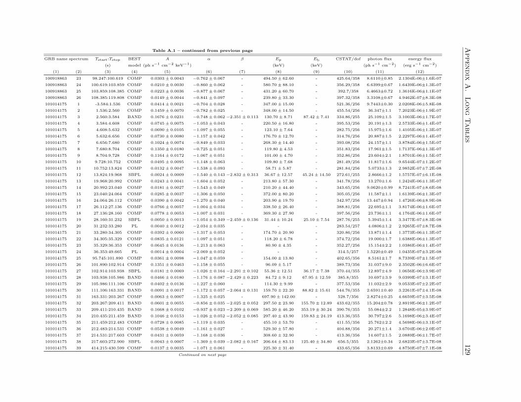
Appendix
A.
Long
Tables
129Table A.1 – continued from previous page
GRB name spectrum Tstart:Tstop BEST A α β Ep Eb CSTAT/dof photon flux energy flux
(s) model (ph s−1 cm−2 keV−1) (keV) (keV) (ph s−1 cm−2) (erg s−1 cm−2)
(1) (2) (3) (4) (5) (6) (7) (8) (9) (10) (11) (12)
100918863 23 98.247:100.619 COMP 0.0303± 0.0043 −0.762± 0.067 - 494.50± 62.60 - 425.64/358 8.6110±0.85 2.1304E-06±1.6E-07
100918863 24 100.619:103.859 COMP 0.0210± 0.0030 −0.860± 0.062 - 580.70± 88.10 - 356.29/358 6.6399±0.67 1.6439E-06±1.3E-07
100918863 25 103.859:108.385 COMP 0.0223± 0.0036 −0.877± 0.067 - 431.20± 60.70 - 392.7/358 6.4663±0.72 1.3616E-06±1.1E-07
100918863 26 108.385:119.808 COMP 0.0149± 0.0044 −0.841± 0.097 - 239.80± 33.30 - 397.32/358 3.3108±0.67 4.9462E-07±8.3E-08
101014175 1 -3.584:1.536 COMP 0.0414± 0.0021 −0.704± 0.028 - 347.00± 15.00 - 521.36/256 9.7443±0.30 2.0208E-06±5.8E-08
101014175 2 1.536:2.560 COMP 0.1459± 0.0070 −0.782± 0.025 - 348.00± 14.50 - 455.54/256 36.347±1.1 7.2023E-06±1.9E-07
101014175 3 2.560:3.584 BAND 0.1676± 0.0231 −0.748± 0.062 −2.351± 0.113 130.70± 8.71 87.42± 7.41 334.86/255 25.109±1.5 3.1003E-06±1.7E-07
101014175 4 3.584:4.608 COMP 0.0745± 0.0075 −1.053± 0.043 - 220.50± 16.80 - 395.53/256 20.191±1.3 2.5733E-06±1.4E-07
101014175 5 4.608:5.632 COMP 0.0690± 0.0105 −1.097± 0.055 - 123.10± 7.64 - 282.75/256 15.975±1.6 1.4105E-06±1.3E-07
101014175 6 5.632:6.656 COMP 0.0730± 0.0080 −1.157± 0.042 - 176.70± 12.70 - 314.76/256 20.887±1.5 2.2297E-06±1.4E-07
101014175 7 6.656:7.680 COMP 0.1024± 0.0074 −0.849± 0.033 - 268.30± 14.40 - 393.08/256 24.157±1.1 3.8784E-06±1.5E-07
101014175 8 7.680:8.704 COMP 0.1350± 0.0180 −0.725± 0.051 - 119.80± 4.53 - 351.83/256 17.961±1.5 1.7137E-06±1.3E-07
101014175 9 8.704:9.728 COMP 0.1164± 0.0172 −1.067± 0.051 - 101.00± 4.70 - 352.86/256 23.604±2.1 1.8701E-06±1.5E-07
101014175 10 9.728:10.752 COMP 0.0495± 0.0095 −1.148± 0.063 - 109.80± 7.68 - 281.49/256 11.817±1.6 9.6544E-07±1.2E-07
101014175 11 10.752:13.824 COMP 0.0132± 0.0047 −1.538± 0.093 - 58.71± 5.87 - 281.84/256 5.0733±1.3 2.9852E-07±7.2E-08
101014175 12 13.824:19.968 SBPL 0.0024± 0.0009 −1.540± 0.143 −2.832± 0.313 36.67± 12.57 45.24± 14.50 272.61/255 2.8666±1.2 1.5757E-07±6.1E-08
101014175 13 19.968:20.992 COMP 0.0243± 0.0041 −1.604± 0.052 - 213.80± 57.30 - 341.78/256 13.270±1.6 1.2424E-06±1.3E-07
101014175 14 20.992:23.040 COMP 0.0181± 0.0027 −1.543± 0.049 - 210.20± 44.40 - 343.65/256 9.0620±0.99 8.7241E-07±8.6E-08
101014175 15 23.040:24.064 COMP 0.0285± 0.0037 −1.306± 0.050 - 372.00± 80.20 - 305.05/256 11.587±1.1 1.6139E-06±1.3E-07
101014175 16 24.064:26.112 COMP 0.0390± 0.0042 −1.270± 0.040 - 203.90± 19.70 - 342.97/256 13.447±0.94 1.4726E-06±8.9E-08
101014175 17 26.112:27.136 COMP 0.0766± 0.0057 −1.004± 0.034 - 338.50± 26.40 - 388.81/256 22.695±1.1 3.8174E-06±1.6E-07
101014175 18 27.136:28.160 COMP 0.0778± 0.0053 −1.007± 0.031 - 369.30± 27.90 - 397.56/256 23.736±1.1 4.1764E-06±1.6E-07
101014175 19 28.160:31.232 SBPL 0.0050± 0.0013 −1.054± 0.349 −2.459± 0.136 31.44± 10.24 25.10± 7.54 287.76/255 5.3945±1.4 3.3477E-07±8.3E-08
101014175 20 31.232:33.280 PL 0.0040± 0.0012 −2.034± 0.035 - - - 283.54/257 4.0806±1.2 2.9265E-07±8.7E-08
101014175 21 33.280:34.305 COMP 0.0392± 0.0060 −1.317± 0.053 - 174.70± 20.90 - 320.86/256 13.871±1.4 1.3773E-06±1.3E-07
101014175 22 34.305:35.329 COMP 0.0835± 0.0121 −1.097± 0.051 - 118.20± 6.78 - 374.72/256 19.000±1.7 1.6388E-06±1.3E-07
101014175 23 35.329:36.353 COMP 0.0645± 0.0136 −1.213± 0.063 - 80.90± 4.35 - 352.27/256 15.154±2.2 1.0386E-06±1.4E-07
101014175 24 36.353:49.665 PL 0.0014± 0.0004 −2.069± 0.052 - - - 314.5/257 1.5220±0.49 1.0435E-07±3.2E-08
101014175 25 95.745:101.890 COMP 0.0361± 0.0098 −1.047± 0.059 - 154.00± 13.80 - 402.65/356 8.5161±1.7 8.7339E-07±1.5E-07
101014175 26 101.890:102.914 COMP 0.1351± 0.0463 −1.158± 0.055 - 96.09± 5.17 - 389.73/356 31.037±9.0 2.3502E-06±6.6E-07
101014175 27 102.914:103.938 SBPL 0.0181± 0.0069 −1.026± 0.164 −2.291± 0.102 55.36± 12.51 36.17± 7.38 370.44/355 12.897±4.9 1.0656E-06±3.9E-07
101014175 28 103.938:105.986 BAND 0.0466± 0.0180 −1.176± 0.087 −2.429± 0.223 84.72± 9.12 67.95± 12.59 385.8/355 10.697±3.9 9.0399E-07±3.1E-07
101014175 29 105.986:111.106 COMP 0.0402± 0.0136 −1.227± 0.060 - 114.30± 9.99 - 377.53/356 11.032±2.9 9.0533E-07±2.2E-07
101014175 30 111.106:163.331 BAND 0.0091± 0.0017 −1.172± 0.057 −2.064± 0.131 159.70± 22.20 88.82± 15.61 544.76/355 2.6591±0.40 3.2261E-07±4.1E-08
101014175 31 163.331:203.267 COMP 0.0063± 0.0007 −1.325± 0.025 - 697.90± 142.00 - 528.7/356 2.8274±0.25 4.6659E-07±3.5E-08
101014175 32 203.267:209.411 BAND 0.0601± 0.0055 −0.856± 0.035 −2.025± 0.052 297.50± 23.90 155.70± 12.89 433.62/355 15.204±0.78 2.8919E-06±1.2E-07
101014175 33 209.411:210.435 BAND 0.1668± 0.0102 −0.937± 0.023 −2.209± 0.069 585.20± 46.20 353.19± 30.24 390.76/355 55.084±2.2 1.2848E-05±3.9E-07
101014175 34 210.435:211.459 BAND 0.1046± 0.0153 −1.026± 0.052 −2.052± 0.085 297.40± 43.90 159.83± 24.19 413.36/355 30.797±2.6 5.1698E-06±3.4E-07
101014175 35 211.459:212.483 COMP 0.0728± 0.0085 −1.119± 0.035 - 455.10± 53.70 - 411.55/356 25.762±2.2 4.5698E-06±3.1E-07
101014175 36 212.483:214.531 COMP 0.0538± 0.0049 −1.161± 0.027 - 529.30± 57.80 - 404.88/356 20.271±1.4 3.6704E-06±2.0E-07
101014175 37 214.531:217.603 COMP 0.0431± 0.0059 −1.168± 0.036 - 308.60± 32.90 - 413.36/356 14.607±1.5 2.0889E-06±1.7E-07
101014175 38 217.603:272.900 SBPL 0.0043± 0.0007 −1.369± 0.039 −2.082± 0.167 206.64± 83.13 125.40± 34.80 656.5/355 2.1262±0.34 2.6823E-07±3.7E-08
101014175 39 414.215:430.599 COMP 0.0137± 0.0035 −1.071± 0.061 - 225.30± 31.40 - 433.65/356 3.8133±0.69 4.8750E-07±7.1E-08
Continued on next page
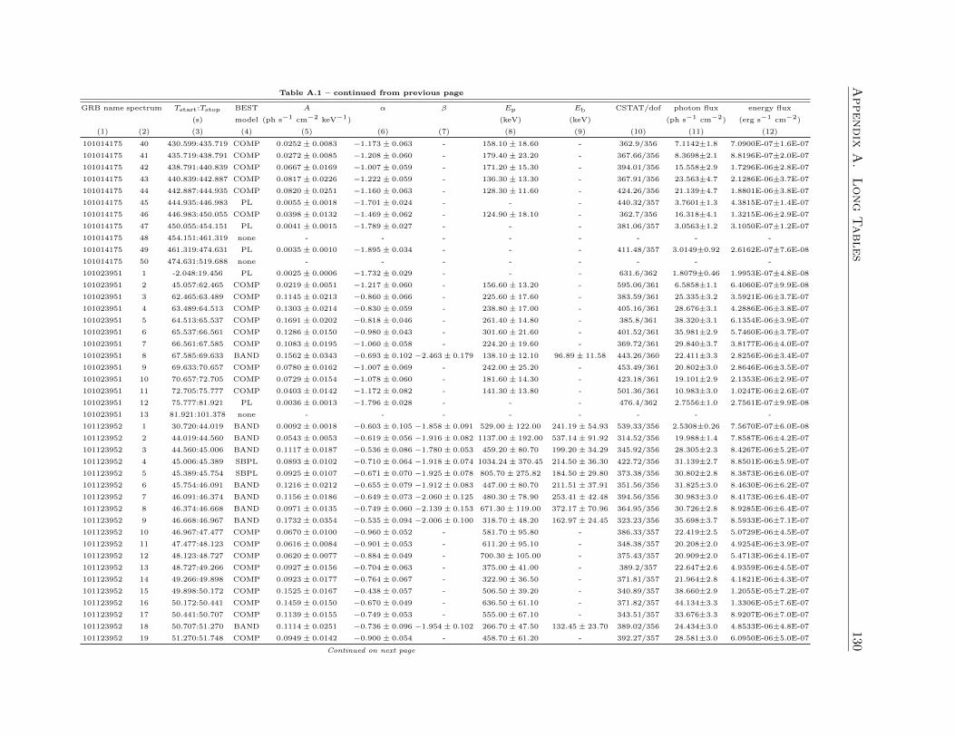
Appendix
A.
Long
Tables
130Table A.1 – continued from previous page
GRB name spectrum Tstart:Tstop BEST A α β Ep Eb CSTAT/dof photon flux energy flux
(s) model (ph s−1 cm−2 keV−1) (keV) (keV) (ph s−1 cm−2) (erg s−1 cm−2)
(1) (2) (3) (4) (5) (6) (7) (8) (9) (10) (11) (12)
101014175 40 430.599:435.719 COMP 0.0252± 0.0083 −1.173± 0.063 - 158.10± 18.60 - 362.9/356 7.1142±1.8 7.0900E-07±1.6E-07
101014175 41 435.719:438.791 COMP 0.0272± 0.0085 −1.208± 0.060 - 179.40± 23.20 - 367.66/356 8.3698±2.1 8.8196E-07±2.0E-07
101014175 42 438.791:440.839 COMP 0.0667± 0.0169 −1.007± 0.059 - 171.20± 15.30 - 394.01/356 15.558±2.9 1.7296E-06±2.8E-07
101014175 43 440.839:442.887 COMP 0.0817± 0.0226 −1.222± 0.059 - 136.30± 13.30 - 367.91/356 23.563±4.7 2.1286E-06±3.7E-07
101014175 44 442.887:444.935 COMP 0.0820± 0.0251 −1.160± 0.063 - 128.30± 11.60 - 424.26/356 21.139±4.7 1.8801E-06±3.8E-07
101014175 45 444.935:446.983 PL 0.0055± 0.0018 −1.701± 0.024 - - - 440.32/357 3.7601±1.3 4.3815E-07±1.4E-07
101014175 46 446.983:450.055 COMP 0.0398± 0.0132 −1.469± 0.062 - 124.90± 18.10 - 362.7/356 16.318±4.1 1.3215E-06±2.9E-07
101014175 47 450.055:454.151 PL 0.0041± 0.0015 −1.789± 0.027 - - - 381.06/357 3.0563±1.2 3.1050E-07±1.2E-07
101014175 48 454.151:461.319 none - - - - - - - -
101014175 49 461.319:474.631 PL 0.0035± 0.0010 −1.895± 0.034 - - - 411.48/357 3.0149±0.92 2.6162E-07±7.6E-08
101014175 50 474.631:519.688 none - - - - - - - -
101023951 1 -2.048:19.456 PL 0.0025± 0.0006 −1.732± 0.029 - - - 631.6/362 1.8079±0.46 1.9953E-07±4.8E-08
101023951 2 45.057:62.465 COMP 0.0219± 0.0051 −1.217± 0.060 - 156.60± 13.20 - 595.06/361 6.5858±1.1 6.4060E-07±9.9E-08
101023951 3 62.465:63.489 COMP 0.1145± 0.0213 −0.860± 0.066 - 225.60± 17.60 - 383.59/361 25.335±3.2 3.5921E-06±3.7E-07
101023951 4 63.489:64.513 COMP 0.1303± 0.0214 −0.830± 0.059 - 238.80± 17.00 - 405.16/361 28.676±3.1 4.2886E-06±3.8E-07
101023951 5 64.513:65.537 COMP 0.1691± 0.0202 −0.818± 0.046 - 261.40± 14.80 - 385.8/361 38.320±3.1 6.1354E-06±3.9E-07
101023951 6 65.537:66.561 COMP 0.1286± 0.0150 −0.980± 0.043 - 301.60± 21.60 - 401.52/361 35.981±2.9 5.7460E-06±3.7E-07
101023951 7 66.561:67.585 COMP 0.1083± 0.0195 −1.060± 0.058 - 224.20± 19.60 - 369.72/361 29.840±3.7 3.8177E-06±4.0E-07
101023951 8 67.585:69.633 BAND 0.1562± 0.0343 −0.693± 0.102 −2.463± 0.179 138.10± 12.10 96.89± 11.58 443.26/360 22.411±3.3 2.8256E-06±3.4E-07
101023951 9 69.633:70.657 COMP 0.0780± 0.0162 −1.007± 0.069 - 242.00± 25.20 - 453.49/361 20.802±3.0 2.8646E-06±3.5E-07
101023951 10 70.657:72.705 COMP 0.0729± 0.0154 −1.078± 0.060 - 181.60± 14.30 - 423.18/361 19.101±2.9 2.1353E-06±2.9E-07
101023951 11 72.705:75.777 COMP 0.0403± 0.0142 −1.172± 0.082 - 141.30± 13.80 - 501.36/361 10.983±3.0 1.0247E-06±2.6E-07
101023951 12 75.777:81.921 PL 0.0036± 0.0013 −1.796± 0.028 - - - 476.4/362 2.7556±1.0 2.7561E-07±9.9E-08
101023951 13 81.921:101.378 none - - - - - - - -
101123952 1 30.720:44.019 BAND 0.0092± 0.0018 −0.603± 0.105 −1.858± 0.091 529.00± 122.00 241.19± 54.93 539.33/356 2.5308±0.26 7.5670E-07±6.0E-08
101123952 2 44.019:44.560 BAND 0.0543± 0.0053 −0.619± 0.056 −1.916± 0.082 1137.00± 192.00 537.14± 91.92 314.52/356 19.988±1.4 7.8587E-06±4.2E-07
101123952 3 44.560:45.006 BAND 0.1117± 0.0187 −0.536± 0.086 −1.780± 0.053 459.20± 80.70 199.20± 34.29 345.92/356 28.305±2.3 8.4267E-06±5.2E-07
101123952 4 45.006:45.389 SBPL 0.0893± 0.0102 −0.710± 0.064 −1.918± 0.074 1034.24± 370.45 214.50± 36.30 422.72/356 31.139±2.7 8.8501E-06±5.9E-07
101123952 5 45.389:45.754 SBPL 0.0925± 0.0107 −0.671± 0.070 −1.925± 0.078 805.70± 275.82 184.50± 29.80 373.38/356 30.802±2.8 8.3873E-06±6.0E-07
101123952 6 45.754:46.091 BAND 0.1216± 0.0212 −0.655± 0.079 −1.912± 0.083 447.00± 80.70 211.51± 37.91 351.56/356 31.825±3.0 8.4630E-06±6.2E-07
101123952 7 46.091:46.374 BAND 0.1156± 0.0186 −0.649± 0.073 −2.060± 0.125 480.30± 78.90 253.41± 42.48 394.56/356 30.983±3.0 8.4173E-06±6.4E-07
101123952 8 46.374:46.668 BAND 0.0971± 0.0135 −0.749± 0.060 −2.139± 0.153 671.30± 119.00 372.17± 70.96 364.95/356 30.726±2.8 8.9285E-06±6.4E-07
101123952 9 46.668:46.967 BAND 0.1732± 0.0354 −0.535± 0.094 −2.006± 0.100 318.70± 48.20 162.97± 24.45 323.23/356 35.698±3.7 8.5933E-06±7.1E-07
101123952 10 46.967:47.477 COMP 0.0670± 0.0100 −0.960± 0.052 - 581.70± 95.80 - 386.33/357 22.419±2.5 5.0729E-06±4.5E-07
101123952 11 47.477:48.123 COMP 0.0616± 0.0084 −0.901± 0.053 - 611.20± 95.10 - 348.38/357 20.208±2.0 4.9254E-06±3.9E-07
101123952 12 48.123:48.727 COMP 0.0620± 0.0077 −0.884± 0.049 - 700.30± 105.00 - 375.43/357 20.909±2.0 5.4713E-06±4.1E-07
101123952 13 48.727:49.266 COMP 0.0927± 0.0156 −0.704± 0.063 - 375.00± 41.00 - 389.2/357 22.647±2.6 4.9359E-06±4.5E-07
101123952 14 49.266:49.898 COMP 0.0923± 0.0177 −0.764± 0.067 - 322.90± 36.50 - 371.81/357 21.964±2.8 4.1821E-06±4.3E-07
101123952 15 49.898:50.172 COMP 0.1525± 0.0167 −0.438± 0.057 - 506.50± 39.20 - 340.89/357 38.660±2.9 1.2055E-05±7.2E-07
101123952 16 50.172:50.441 COMP 0.1459± 0.0150 −0.670± 0.049 - 636.50± 61.10 - 371.82/357 44.134±3.3 1.3306E-05±7.6E-07
101123952 17 50.441:50.707 COMP 0.1139± 0.0155 −0.749± 0.053 - 555.00± 67.10 - 343.51/357 33.676±3.3 8.9207E-06±7.0E-07
101123952 18 50.707:51.270 BAND 0.1114± 0.0251 −0.736± 0.096 −1.954± 0.102 266.70± 47.50 132.45± 23.70 389.02/356 24.434±3.0 4.8533E-06±4.8E-07
101123952 19 51.270:51.748 COMP 0.0949± 0.0142 −0.900± 0.054 - 458.70± 61.20 - 392.27/357 28.581±3.0 6.0950E-06±5.0E-07
Continued on next page
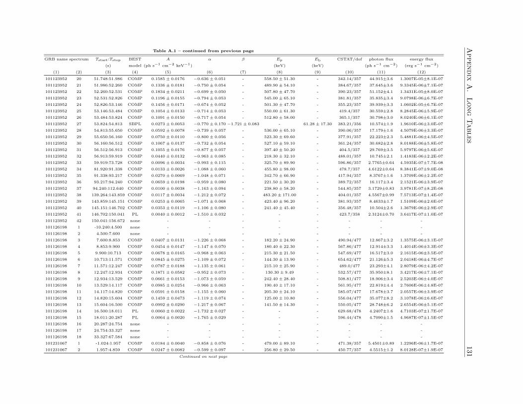
Appendix
A.
Long
Tables
131Table A.1 – continued from previous page
GRB name spectrum Tstart:Tstop BEST A α β Ep Eb CSTAT/dof photon flux energy flux
(s) model (ph s−1 cm−2 keV−1) (keV) (keV) (ph s−1 cm−2) (erg s−1 cm−2)
(1) (2) (3) (4) (5) (6) (7) (8) (9) (10) (11) (12)
101123952 20 51.748:51.986 COMP 0.1585± 0.0176 −0.636± 0.051 - 558.50± 51.30 - 342.14/357 44.915±3.6 1.3007E-05±8.1E-07
101123952 21 51.986:52.260 COMP 0.1336± 0.0181 −0.750± 0.054 - 489.90± 54.10 - 384.67/357 37.645±3.6 9.3345E-06±7.1E-07
101123952 22 52.260:52.531 COMP 0.1834± 0.0211 −0.699± 0.050 - 507.80± 47.70 - 390.23/357 51.152±4.1 1.3431E-05±8.0E-07
101123952 23 52.531:52.826 COMP 0.1196± 0.0155 −0.794± 0.053 - 545.00± 65.10 - 381.81/357 35.835±3.4 9.0798E-06±6.7E-07
101123952 24 52.826:53.146 COMP 0.1456± 0.0171 −0.674± 0.052 - 501.30± 47.70 - 355.23/357 39.939±3.3 1.0602E-05±6.7E-07
101123952 25 53.146:53.484 COMP 0.1054± 0.0133 −0.714± 0.053 - 550.00± 61.30 - 419.4/357 30.559±2.8 8.2845E-06±5.9E-07
101123952 26 53.484:53.824 COMP 0.1091± 0.0150 −0.717± 0.054 - 512.80± 58.00 - 365.1/357 30.798±3.0 8.0240E-06±6.1E-07
101123952 27 53.824:54.813 SBPL 0.0273± 0.0053 −0.770± 0.170 −1.721± 0.083 - 61.28± 17.30 383.21/356 10.574±1.9 1.9610E-06±3.0E-07
101123952 28 54.813:55.650 COMP 0.0592± 0.0078 −0.739± 0.057 - 536.00± 65.10 - 390.06/357 17.179±1.6 4.5079E-06±3.3E-07
101123952 29 55.650:56.160 COMP 0.0750± 0.0110 −0.800± 0.056 - 523.30± 69.60 - 377.91/357 22.223±2.3 5.4881E-06±4.5E-07
101123952 30 56.160:56.512 COMP 0.1067± 0.0137 −0.732± 0.054 - 527.10± 59.10 - 361.24/357 30.682±2.8 8.0188E-06±5.8E-07
101123952 31 56.512:56.913 COMP 0.1055± 0.0176 −0.877± 0.057 - 397.40± 50.20 - 404.5/357 29.769±3.5 5.9797E-06±5.6E-07
101123952 32 56.913:59.919 COMP 0.0440± 0.0132 −0.963± 0.085 - 218.30± 32.10 - 488.01/357 10.745±2.1 1.4183E-06±2.2E-07
101123952 33 59.919:73.728 COMP 0.0096± 0.0034 −0.993± 0.115 - 325.70± 89.90 - 596.86/357 2.7765±0.64 4.5935E-07±7.7E-08
101123952 34 81.920:91.338 COMP 0.0133± 0.0026 −1.088± 0.060 - 455.80± 98.00 - 478.7/357 4.6122±0.64 8.3841E-07±9.0E-08
101123952 35 91.338:93.217 COMP 0.0270± 0.0069 −1.048± 0.071 - 342.70± 66.90 - 417.94/357 8.3767±1.6 1.3709E-06±2.2E-07
101123952 36 93.217:94.240 COMP 0.0659± 0.0198 −0.959± 0.080 - 221.50± 30.20 - 389.72/357 16.117±3.4 2.1521E-06±3.9E-07
101123952 37 94.240:112.640 COMP 0.0100± 0.0038 −1.163± 0.094 - 238.80± 58.20 - 544.85/357 3.1729±0.83 3.9781E-07±8.2E-08
101123952 38 139.264:143.859 COMP 0.0117± 0.0034 −1.212± 0.072 - 483.20± 171.00 - 404.01/357 4.5567±0.99 7.5713E-07±1.4E-07
101123952 39 143.859:145.151 COMP 0.0253± 0.0065 −1.071± 0.068 - 423.40± 96.20 - 381.93/357 8.4633±1.7 1.5109E-06±2.6E-07
101123952 40 145.151:146.702 COMP 0.0353± 0.0119 −1.106± 0.080 - 241.40± 45.40 - 356.48/357 10.504±2.6 1.3679E-06±2.9E-07
101123952 41 146.702:150.041 PL 0.0040± 0.0012 −1.510± 0.032 - - - 423.7/358 2.3124±0.70 3.6417E-07±1.0E-07
101123952 42 150.041:156.672 none - - - - - - - -
101126198 1 -10.240:4.500 none - - - - - - - -
101126198 2 4.500:7.600 none - - - - - - - -
101126198 3 7.600:8.853 COMP 0.0407± 0.0131 −1.226± 0.068 - 182.20± 24.90 - 490.94/477 12.867±3.2 1.3575E-06±3.1E-07
101126198 4 8.853:9.900 COMP 0.0454± 0.0147 −1.147± 0.070 - 180.40± 22.30 - 567.86/477 12.914±3.3 1.4014E-06±3.3E-07
101126198 5 9.900:10.713 COMP 0.0678± 0.0165 −0.968± 0.063 - 215.30± 21.50 - 547.69/477 16.517±3.0 2.1615E-06±3.5E-07
101126198 6 10.713:11.571 COMP 0.0845± 0.0275 −1.109± 0.072 - 144.30± 13.90 - 654.62/477 21.126±5.3 2.0418E-06±4.7E-07
101126198 7 11.571:12.247 COMP 0.0787± 0.0188 −1.135± 0.061 - 215.10± 25.90 - 489.0/477 23.293±4.1 2.8079E-06±4.2E-07
101126198 8 12.247:12.934 COMP 0.1871± 0.0582 −0.952± 0.073 - 130.30± 9.49 - 532.57/477 35.950±8.1 3.4217E-06±7.1E-07
101126198 9 12.934:13.529 COMP 0.0661± 0.0153 −1.073± 0.059 - 242.40± 28.40 - 508.81/477 18.906±3.4 2.5203E-06±4.0E-07
101126198 10 13.529:14.117 COMP 0.0985± 0.0254 −0.966± 0.063 - 190.40± 17.10 - 561.95/477 22.819±4.4 2.7606E-06±4.8E-07
101126198 11 14.117:14.820 COMP 0.0591± 0.0158 −1.155± 0.060 - 205.30± 24.10 - 585.07/477 17.678±3.7 2.0557E-06±3.9E-07
101126198 12 14.820:15.604 COMP 0.1459± 0.0473 −1.119± 0.074 - 125.00± 10.80 - 556.04/477 35.077±8.2 3.1078E-06±6.6E-07
101126198 13 15.604:16.500 COMP 0.0992± 0.0290 −1.217± 0.067 - 141.50± 14.30 - 550.05/477 28.748±6.2 2.6554E-06±5.1E-07
101126198 14 16.500:18.011 PL 0.0060± 0.0022 −1.732± 0.027 - - - 629.68/478 4.2407±1.6 4.7103E-07±1.7E-07
101126198 15 18.011:20.287 PL 0.0064± 0.0020 −1.765± 0.029 - - - 596.44/478 4.7090±1.5 4.9687E-07±1.5E-07
101126198 16 20.287:24.754 none - - - - - - - -
101126198 17 24.754:33.327 none - - - - - - - -
101126198 18 33.327:67.584 none - - - - - - - -
101231067 1 -1.024:1.957 COMP 0.0184± 0.0040 −0.858± 0.076 - 479.00± 89.10 - 471.38/357 5.4501±0.89 1.2296E-06±1.7E-07
101231067 2 1.957:4.859 COMP 0.0247± 0.0082 −0.599± 0.097 - 256.80± 29.50 - 450.77/357 4.5515±1.2 8.0128E-07±1.9E-07
Continued on next page
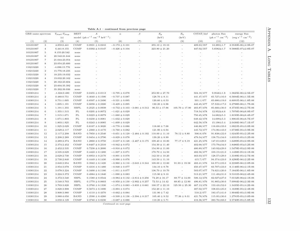
Appendix
A.
Long
Tables
132Table A.1 – continued from previous page
GRB name spectrum Tstart:Tstop BEST A α β Ep Eb CSTAT/dof photon flux energy flux
(s) model (ph s−1 cm−2 keV−1) (keV) (keV) (ph s−1 cm−2) (erg s−1 cm−2)
(1) (2) (3) (4) (5) (6) (7) (8) (9) (10) (11) (12)
101231067 3 4.859:6.441 COMP 0.0931± 0.0210 −0.172± 0.101 - 255.10± 19.10 - 409.63/357 12.289±1.7 2.5530E-06±2.9E-07
101231067 4 6.441:8.155 COMP 0.0392± 0.0147 −0.426± 0.104 - 223.80± 21.20 - 447.02/357 5.6582±1.7 9.5886E-07±2.8E-07
101231067 5 8.155:20.542 none - - - - - - - -
101231067 6 20.542:21.644 none - - - - - - - -
101231067 7 21.644:23.054 none - - - - - - - -
101231067 8 23.054:25.600 none - - - - - - - -
110213220 1 -4.096:15.776 none - - - - - - - -
110213220 2 15.776:18.235 none - - - - - - - -
110213220 3 18.235:19.032 none - - - - - - - -
110213220 4 19.032:20.162 none - - - - - - - -
110213220 5 20.162:23.604 none - - - - - - - -
110213220 6 23.604:35.392 none - - - - - - - -
110213220 7 35.392:39.936 none - - - - - - - -
110301214 1 -1.024:0.480 COMP 0.0455± 0.0113 −0.795± 0.078 - 253.90± 27.70 - 504.18/477 9.9546±1.8 1.5825E-06±2.5E-07
110301214 2 0.480:0.751 COMP 0.4640± 0.1590 −0.737± 0.087 - 128.70± 8.11 - 441.47/477 65.727±16.0 6.5694E-06±1.5E-06
110301214 3 0.751:1.005 COMP 0.6507± 0.2490 −0.521± 0.095 - 120.60± 6.53 - 501.1/477 65.680±19.0 6.6091E-06±1.8E-06
110301214 4 1.005:1.191 COMP 0.6058± 0.2300 −0.429± 0.095 - 130.20± 6.96 - 442.45/477 57.532±17.0 6.2798E-06±1.7E-06
110301214 5 1.191:1.355 SBPL 0.2525± 0.0939 −0.732± 0.103 −3.681± 0.512 96.53± 17.96 105.70± 17.90 483.87/476 85.666±30.0 8.3735E-06±2.7E-06
110301214 6 1.355:1.515 PL 0.0205± 0.0072 −1.621± 0.029 - - - 718.54/478 12.952±4.6 1.7076E-06±6.0E-07
110301214 7 1.515:1.671 PL 0.0223± 0.0079 −1.660± 0.029 - - - 750.45/478 14.682±5.3 1.8193E-06±6.4E-07
110301214 8 1.671:1.803 PL 0.0230± 0.0081 −1.632± 0.029 - - - 649.42/478 14.699±5.3 1.9061E-06±6.7E-07
110301214 9 1.803:1.925 PL 0.0243± 0.0085 −1.609± 0.029 - - - 642.58/478 15.198±5.4 2.0436E-06±7.1E-07
110301214 10 1.925:2.029 COMP 0.8167± 0.3020 −0.778± 0.086 - 118.80± 7.06 - 446.88/477 116.69±33.0 1.0921E-05±3.0E-06
110301214 11 2.029:2.117 COMP 1.2360± 0.4170 −0.760± 0.082 - 121.90± 6.94 - 445.72/477 174.96±43.0 1.6738E-05±3.9E-06
110301214 12 2.117:2.208 BAND 0.7850± 0.2540 −0.651± 0.129 −2.484± 0.192 110.00± 11.10 78.12± 9.80 506.8/476 91.838±22.0 1.0243E-05±2.2E-06
110301214 13 2.208:2.289 COMP 0.9454± 0.2790 −0.829± 0.078 - 139.20± 8.99 - 479.54/477 158.75±34.0 1.6331E-05±3.2E-06
110301214 14 2.289:2.374 BAND 1.2860± 0.3750 −0.637± 0.128 −2.467± 0.175 109.40± 10.80 77.17± 9.19 421.25/476 147.01±29.0 1.6499E-05±2.9E-06
110301214 15 2.374:2.452 COMP 0.8467± 0.2310 −0.942± 0.072 - 154.30± 11.40 - 402.68/477 173.79±34.0 1.8486E-05±3.2E-06
110301214 16 2.452:2.535 COMP 0.7238± 0.2000 −0.916± 0.072 - 154.90± 11.00 - 480.89/477 143.92±29.0 1.5479E-05±2.9E-06
110301214 17 2.535:2.629 COMP 0.4422± 0.1200 −1.007± 0.071 - 170.70± 14.50 - 482.56/477 103.15±21.0 1.1436E-05±2.1E-06
110301214 18 2.629:2.730 COMP 0.6953± 0.2170 −0.891± 0.078 - 142.50± 10.20 - 463.03/477 128.57±29.0 1.3189E-05±2.7E-06
110301214 19 2.730:2.840 COMP 0.4449± 0.1430 −0.990± 0.076 - 143.50± 11.10 - 415.7/477 94.374±23.0 9.4290E-06±2.2E-06
110301214 20 2.840:2.954 BAND 0.3562± 0.1420 −0.960± 0.116 −2.643± 0.344 109.00± 12.80 91.93± 19.58 483.41/476 64.571±23.0 6.2238E-06±2.0E-06
110301214 21 2.954:3.078 COMP 0.4316± 0.1480 −0.948± 0.077 - 134.10± 9.78 - 450.47/477 83.707±23.0 8.1146E-06±2.1E-06
110301214 22 3.078:3.224 COMP 0.3490± 0.1180 −1.011± 0.077 - 136.70± 10.70 - 503.07/477 74.621±20.0 7.1843E-06±1.8E-06
110301214 23 3.224:3.372 COMP 0.4984± 0.1840 −1.090± 0.083 - 115.90± 9.10 - 513.21/477 111.49±31.0 9.5101E-06±2.4E-06
110301214 24 3.372:3.540 SBPL 0.1580± 0.0544 −0.984± 0.132 −2.814± 0.256 74.29± 16.17 68.77± 14.00 506.12/476 82.027±27.0 7.0152E-06±2.1E-06
110301214 25 3.540:3.703 SBPL 0.1770± 0.0603 −0.950± 0.130 −2.902± 0.257 72.53± 14.42 68.85± 12.90 496.81/476 91.885±30.0 7.6994E-06±2.3E-06
110301214 26 3.703:3.820 SBPL 0.3760± 0.1330 −1.074± 0.083 −3.833± 0.661 100.57± 22.10 125.50± 25.30 467.13/476 153.43±52.0 1.3435E-05±4.2E-06
110301214 27 3.820:3.908 COMP 0.5673± 0.1690 −0.894± 0.074 - 152.20± 11.10 - 487.02/477 108.65±25.0 1.1639E-05±2.4E-06
110301214 28 3.908:3.980 COMP 1.4110± 0.4370 −0.662± 0.084 - 131.90± 7.42 - 510.2/477 183.47±41.0 1.9046E-05±3.9E-06
110301214 29 3.980:4.050 BAND 1.2590± 0.4280 −0.509± 0.136 −2.594± 0.217 105.40± 9.52 77.36± 9.31 421.76/476 115.95±30.0 1.2791E-05±3.0E-06
110301214 30 4.050:4.129 COMP 2.3740± 0.8230 −0.687± 0.088 - 110.20± 5.71 - 416.36/477 283.76±68.0 2.5740E-05±5.8E-06
Continued on next page
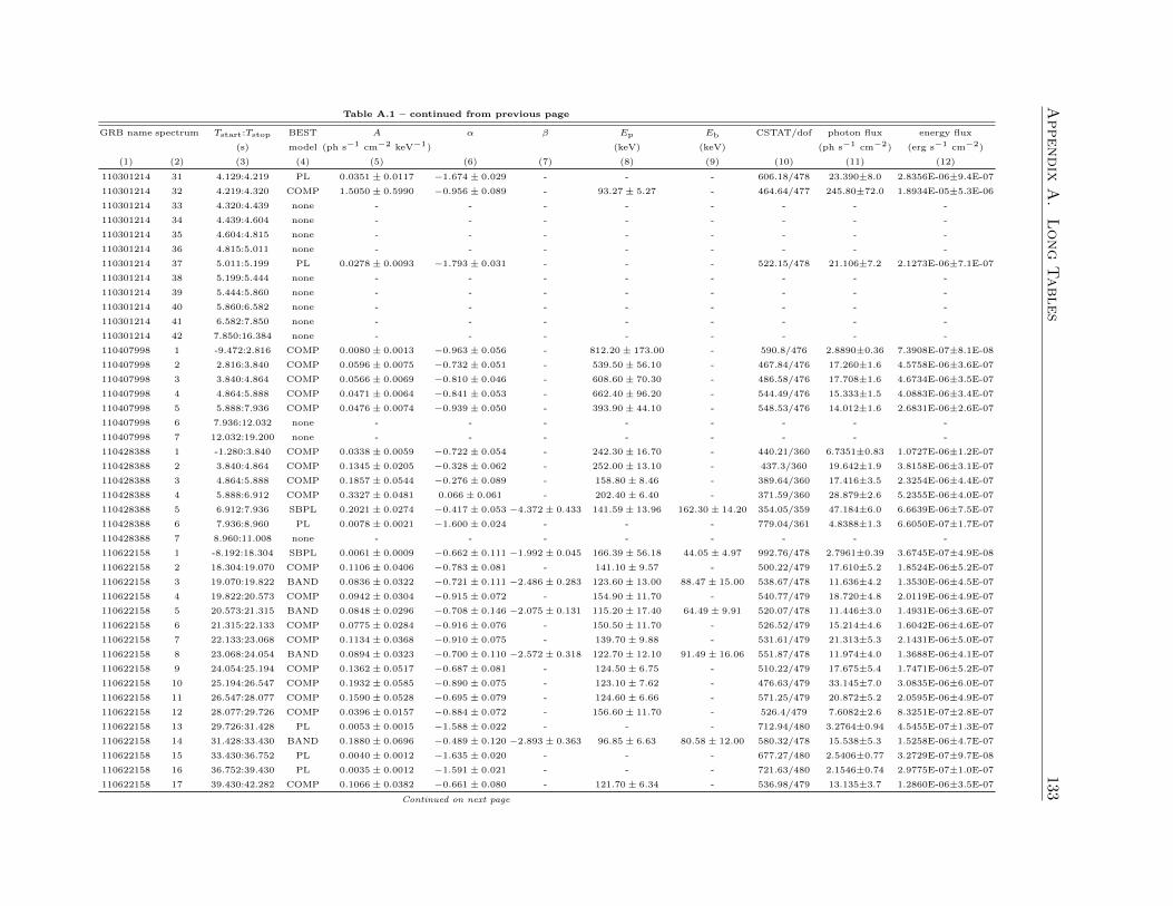
Appendix
A.
Long
Tables
133Table A.1 – continued from previous page
GRB name spectrum Tstart:Tstop BEST A α β Ep Eb CSTAT/dof photon flux energy flux
(s) model (ph s−1 cm−2 keV−1) (keV) (keV) (ph s−1 cm−2) (erg s−1 cm−2)
(1) (2) (3) (4) (5) (6) (7) (8) (9) (10) (11) (12)
110301214 31 4.129:4.219 PL 0.0351± 0.0117 −1.674± 0.029 - - - 606.18/478 23.390±8.0 2.8356E-06±9.4E-07
110301214 32 4.219:4.320 COMP 1.5050± 0.5990 −0.956± 0.089 - 93.27± 5.27 - 464.64/477 245.80±72.0 1.8934E-05±5.3E-06
110301214 33 4.320:4.439 none - - - - - - - -
110301214 34 4.439:4.604 none - - - - - - - -
110301214 35 4.604:4.815 none - - - - - - - -
110301214 36 4.815:5.011 none - - - - - - - -
110301214 37 5.011:5.199 PL 0.0278± 0.0093 −1.793± 0.031 - - - 522.15/478 21.106±7.2 2.1273E-06±7.1E-07
110301214 38 5.199:5.444 none - - - - - - - -
110301214 39 5.444:5.860 none - - - - - - - -
110301214 40 5.860:6.582 none - - - - - - - -
110301214 41 6.582:7.850 none - - - - - - - -
110301214 42 7.850:16.384 none - - - - - - - -
110407998 1 -9.472:2.816 COMP 0.0080± 0.0013 −0.963± 0.056 - 812.20± 173.00 - 590.8/476 2.8890±0.36 7.3908E-07±8.1E-08
110407998 2 2.816:3.840 COMP 0.0596± 0.0075 −0.732± 0.051 - 539.50± 56.10 - 467.84/476 17.260±1.6 4.5758E-06±3.6E-07
110407998 3 3.840:4.864 COMP 0.0566± 0.0069 −0.810± 0.046 - 608.60± 70.30 - 486.58/476 17.708±1.6 4.6734E-06±3.5E-07
110407998 4 4.864:5.888 COMP 0.0471± 0.0064 −0.841± 0.053 - 662.40± 96.20 - 544.49/476 15.333±1.5 4.0883E-06±3.4E-07
110407998 5 5.888:7.936 COMP 0.0476± 0.0074 −0.939± 0.050 - 393.90± 44.10 - 548.53/476 14.012±1.6 2.6831E-06±2.6E-07
110407998 6 7.936:12.032 none - - - - - - - -
110407998 7 12.032:19.200 none - - - - - - - -
110428388 1 -1.280:3.840 COMP 0.0338± 0.0059 −0.722± 0.054 - 242.30± 16.70 - 440.21/360 6.7351±0.83 1.0727E-06±1.2E-07
110428388 2 3.840:4.864 COMP 0.1345± 0.0205 −0.328± 0.062 - 252.00± 13.10 - 437.3/360 19.642±1.9 3.8158E-06±3.1E-07
110428388 3 4.864:5.888 COMP 0.1857± 0.0544 −0.276± 0.089 - 158.80± 8.46 - 389.64/360 17.416±3.5 2.3254E-06±4.4E-07
110428388 4 5.888:6.912 COMP 0.3327± 0.0481 0.066± 0.061 - 202.40± 6.40 - 371.59/360 28.879±2.6 5.2355E-06±4.0E-07
110428388 5 6.912:7.936 SBPL 0.2021± 0.0274 −0.417± 0.053 −4.372± 0.433 141.59± 13.96 162.30± 14.20 354.05/359 47.184±6.0 6.6639E-06±7.5E-07
110428388 6 7.936:8.960 PL 0.0078± 0.0021 −1.600± 0.024 - - - 779.04/361 4.8388±1.3 6.6050E-07±1.7E-07
110428388 7 8.960:11.008 none - - - - - - - -
110622158 1 -8.192:18.304 SBPL 0.0061± 0.0009 −0.662± 0.111 −1.992± 0.045 166.39± 56.18 44.05± 4.97 992.76/478 2.7961±0.39 3.6745E-07±4.9E-08
110622158 2 18.304:19.070 COMP 0.1106± 0.0406 −0.783± 0.081 - 141.10± 9.57 - 500.22/479 17.610±5.2 1.8524E-06±5.2E-07
110622158 3 19.070:19.822 BAND 0.0836± 0.0322 −0.721± 0.111 −2.486± 0.283 123.60± 13.00 88.47± 15.00 538.67/478 11.636±4.2 1.3530E-06±4.5E-07
110622158 4 19.822:20.573 COMP 0.0942± 0.0304 −0.915± 0.072 - 154.90± 11.70 - 540.77/479 18.720±4.8 2.0119E-06±4.9E-07
110622158 5 20.573:21.315 BAND 0.0848± 0.0296 −0.708± 0.146 −2.075± 0.131 115.20± 17.40 64.49± 9.91 520.07/478 11.446±3.0 1.4931E-06±3.6E-07
110622158 6 21.315:22.133 COMP 0.0775± 0.0284 −0.916± 0.076 - 150.50± 11.70 - 526.52/479 15.214±4.6 1.6042E-06±4.6E-07
110622158 7 22.133:23.068 COMP 0.1134± 0.0368 −0.910± 0.075 - 139.70± 9.88 - 531.61/479 21.313±5.3 2.1431E-06±5.0E-07
110622158 8 23.068:24.054 BAND 0.0894± 0.0323 −0.700± 0.110 −2.572± 0.318 122.70± 12.10 91.49± 16.06 551.87/478 11.974±4.0 1.3688E-06±4.1E-07
110622158 9 24.054:25.194 COMP 0.1362± 0.0517 −0.687± 0.081 - 124.50± 6.75 - 510.22/479 17.675±5.4 1.7471E-06±5.2E-07
110622158 10 25.194:26.547 COMP 0.1932± 0.0585 −0.890± 0.075 - 123.10± 7.62 - 476.63/479 33.145±7.0 3.0835E-06±6.0E-07
110622158 11 26.547:28.077 COMP 0.1590± 0.0528 −0.695± 0.079 - 124.60± 6.66 - 571.25/479 20.872±5.2 2.0595E-06±4.9E-07
110622158 12 28.077:29.726 COMP 0.0396± 0.0157 −0.884± 0.072 - 156.60± 11.70 - 526.4/479 7.6082±2.6 8.3251E-07±2.8E-07
110622158 13 29.726:31.428 PL 0.0053± 0.0015 −1.588± 0.022 - - - 712.94/480 3.2764±0.94 4.5455E-07±1.3E-07
110622158 14 31.428:33.430 BAND 0.1880± 0.0696 −0.489± 0.120 −2.893± 0.363 96.85± 6.63 80.58± 12.00 580.32/478 15.538±5.3 1.5258E-06±4.7E-07
110622158 15 33.430:36.752 PL 0.0040± 0.0012 −1.635± 0.020 - - - 677.27/480 2.5406±0.77 3.2729E-07±9.7E-08
110622158 16 36.752:39.430 PL 0.0035± 0.0012 −1.591± 0.021 - - - 721.63/480 2.1546±0.74 2.9775E-07±1.0E-07
110622158 17 39.430:42.282 COMP 0.1066± 0.0382 −0.661± 0.080 - 121.70± 6.34 - 536.98/479 13.135±3.7 1.2860E-06±3.5E-07
Continued on next page
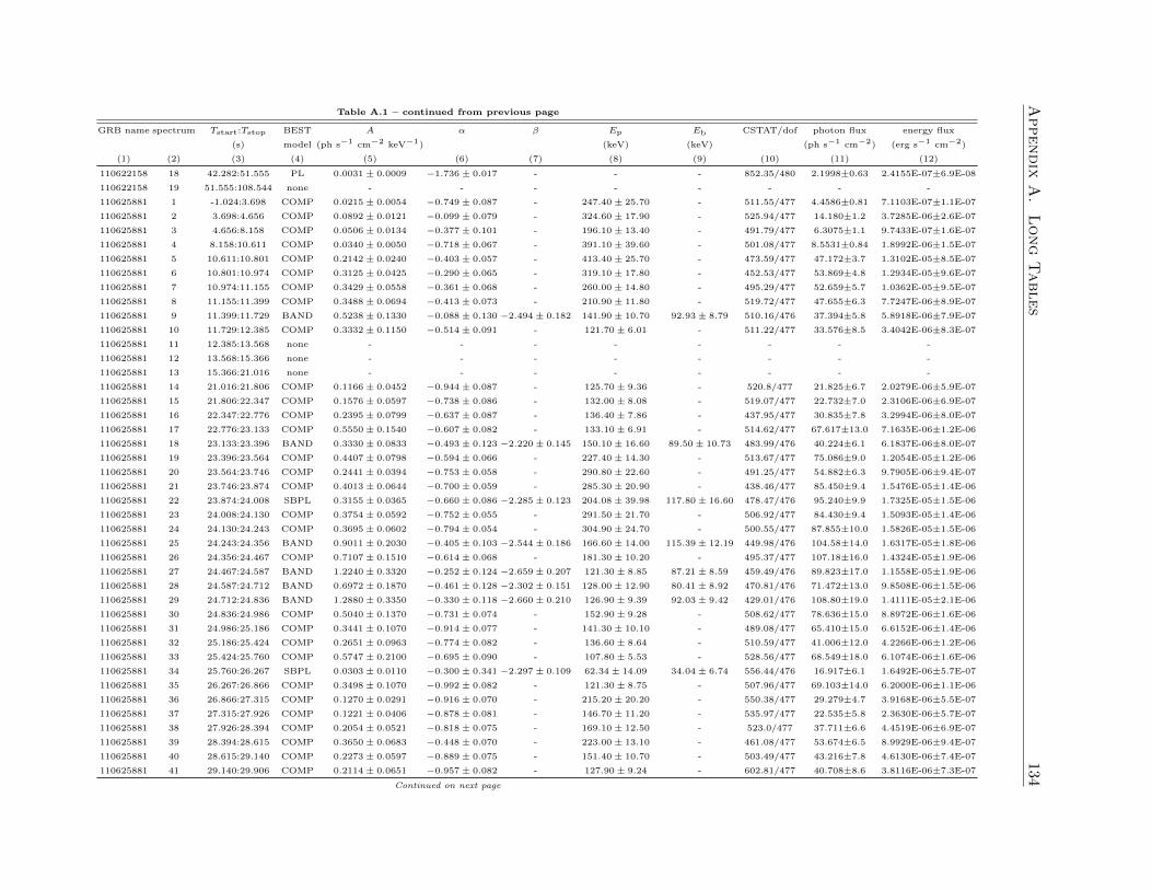
Appendix
A.
Long
Tables
134Table A.1 – continued from previous page
GRB name spectrum Tstart:Tstop BEST A α β Ep Eb CSTAT/dof photon flux energy flux
(s) model (ph s−1 cm−2 keV−1) (keV) (keV) (ph s−1 cm−2) (erg s−1 cm−2)
(1) (2) (3) (4) (5) (6) (7) (8) (9) (10) (11) (12)
110622158 18 42.282:51.555 PL 0.0031± 0.0009 −1.736± 0.017 - - - 852.35/480 2.1998±0.63 2.4155E-07±6.9E-08
110622158 19 51.555:108.544 none - - - - - - - -
110625881 1 -1.024:3.698 COMP 0.0215± 0.0054 −0.749± 0.087 - 247.40± 25.70 - 511.55/477 4.4586±0.81 7.1103E-07±1.1E-07
110625881 2 3.698:4.656 COMP 0.0892± 0.0121 −0.099± 0.079 - 324.60± 17.90 - 525.94/477 14.180±1.2 3.7285E-06±2.6E-07
110625881 3 4.656:8.158 COMP 0.0506± 0.0134 −0.377± 0.101 - 196.10± 13.40 - 491.79/477 6.3075±1.1 9.7433E-07±1.6E-07
110625881 4 8.158:10.611 COMP 0.0340± 0.0050 −0.718± 0.067 - 391.10± 39.60 - 501.08/477 8.5531±0.84 1.8992E-06±1.5E-07
110625881 5 10.611:10.801 COMP 0.2142± 0.0240 −0.403± 0.057 - 413.40± 25.70 - 473.59/477 47.172±3.7 1.3102E-05±8.5E-07
110625881 6 10.801:10.974 COMP 0.3125± 0.0425 −0.290± 0.065 - 319.10± 17.80 - 452.53/477 53.869±4.8 1.2934E-05±9.6E-07
110625881 7 10.974:11.155 COMP 0.3429± 0.0558 −0.361± 0.068 - 260.00± 14.80 - 495.29/477 52.659±5.7 1.0362E-05±9.5E-07
110625881 8 11.155:11.399 COMP 0.3488± 0.0694 −0.413± 0.073 - 210.90± 11.80 - 519.72/477 47.655±6.3 7.7247E-06±8.9E-07
110625881 9 11.399:11.729 BAND 0.5238± 0.1330 −0.088± 0.130 −2.494± 0.182 141.90± 10.70 92.93± 8.79 510.16/476 37.394±5.8 5.8918E-06±7.9E-07
110625881 10 11.729:12.385 COMP 0.3332± 0.1150 −0.514± 0.091 - 121.70± 6.01 - 511.22/477 33.576±8.5 3.4042E-06±8.3E-07
110625881 11 12.385:13.568 none - - - - - - - -
110625881 12 13.568:15.366 none - - - - - - - -
110625881 13 15.366:21.016 none - - - - - - - -
110625881 14 21.016:21.806 COMP 0.1166± 0.0452 −0.944± 0.087 - 125.70± 9.36 - 520.8/477 21.825±6.7 2.0279E-06±5.9E-07
110625881 15 21.806:22.347 COMP 0.1576± 0.0597 −0.738± 0.086 - 132.00± 8.08 - 519.07/477 22.732±7.0 2.3106E-06±6.9E-07
110625881 16 22.347:22.776 COMP 0.2395± 0.0799 −0.637± 0.087 - 136.40± 7.86 - 437.95/477 30.835±7.8 3.2994E-06±8.0E-07
110625881 17 22.776:23.133 COMP 0.5550± 0.1540 −0.607± 0.082 - 133.10± 6.91 - 514.62/477 67.617±13.0 7.1635E-06±1.2E-06
110625881 18 23.133:23.396 BAND 0.3330± 0.0833 −0.493± 0.123 −2.220± 0.145 150.10± 16.60 89.50± 10.73 483.99/476 40.224±6.1 6.1837E-06±8.0E-07
110625881 19 23.396:23.564 COMP 0.4407± 0.0798 −0.594± 0.066 - 227.40± 14.30 - 513.67/477 75.086±9.0 1.2054E-05±1.2E-06
110625881 20 23.564:23.746 COMP 0.2441± 0.0394 −0.753± 0.058 - 290.80± 22.60 - 491.25/477 54.882±6.3 9.7905E-06±9.4E-07
110625881 21 23.746:23.874 COMP 0.4013± 0.0644 −0.700± 0.059 - 285.30± 20.90 - 438.46/477 85.450±9.4 1.5476E-05±1.4E-06
110625881 22 23.874:24.008 SBPL 0.3155± 0.0365 −0.660± 0.086 −2.285± 0.123 204.08± 39.98 117.80± 16.60 478.47/476 95.240±9.9 1.7325E-05±1.5E-06
110625881 23 24.008:24.130 COMP 0.3754± 0.0592 −0.752± 0.055 - 291.50± 21.70 - 506.92/477 84.430±9.4 1.5093E-05±1.4E-06
110625881 24 24.130:24.243 COMP 0.3695± 0.0602 −0.794± 0.054 - 304.90± 24.70 - 500.55/477 87.855±10.0 1.5826E-05±1.5E-06
110625881 25 24.243:24.356 BAND 0.9011± 0.2030 −0.405± 0.103 −2.544± 0.186 166.60± 14.00 115.39± 12.19 449.98/476 104.58±14.0 1.6317E-05±1.8E-06
110625881 26 24.356:24.467 COMP 0.7107± 0.1510 −0.614± 0.068 - 181.30± 10.20 - 495.37/477 107.18±16.0 1.4324E-05±1.9E-06
110625881 27 24.467:24.587 BAND 1.2240± 0.3320 −0.252± 0.124 −2.659± 0.207 121.30± 8.85 87.21± 8.59 459.49/476 89.823±17.0 1.1558E-05±1.9E-06
110625881 28 24.587:24.712 BAND 0.6972± 0.1870 −0.461± 0.128 −2.302± 0.151 128.00± 12.90 80.41± 8.92 470.81/476 71.472±13.0 9.8508E-06±1.5E-06
110625881 29 24.712:24.836 BAND 1.2880± 0.3350 −0.330± 0.118 −2.660± 0.210 126.90± 9.39 92.03± 9.42 429.01/476 108.80±19.0 1.4111E-05±2.1E-06
110625881 30 24.836:24.986 COMP 0.5040± 0.1370 −0.731± 0.074 - 152.90± 9.28 - 508.62/477 78.636±15.0 8.8972E-06±1.6E-06
110625881 31 24.986:25.186 COMP 0.3441± 0.1070 −0.914± 0.077 - 141.30± 10.10 - 489.08/477 65.410±15.0 6.6152E-06±1.4E-06
110625881 32 25.186:25.424 COMP 0.2651± 0.0963 −0.774± 0.082 - 136.60± 8.64 - 510.59/477 41.006±12.0 4.2266E-06±1.2E-06
110625881 33 25.424:25.760 COMP 0.5747± 0.2100 −0.695± 0.090 - 107.80± 5.53 - 528.56/477 68.549±18.0 6.1074E-06±1.6E-06
110625881 34 25.760:26.267 SBPL 0.0303± 0.0110 −0.300± 0.341 −2.297± 0.109 62.34± 14.09 34.04± 6.74 556.44/476 16.917±6.1 1.6492E-06±5.7E-07
110625881 35 26.267:26.866 COMP 0.3498± 0.1070 −0.992± 0.082 - 121.30± 8.75 - 507.96/477 69.103±14.0 6.2000E-06±1.1E-06
110625881 36 26.866:27.315 COMP 0.1270± 0.0291 −0.916± 0.070 - 215.20± 20.20 - 550.38/477 29.279±4.7 3.9168E-06±5.5E-07
110625881 37 27.315:27.926 COMP 0.1221± 0.0406 −0.878± 0.081 - 146.70± 11.20 - 535.97/477 22.535±5.8 2.3630E-06±5.7E-07
110625881 38 27.926:28.394 COMP 0.2054± 0.0521 −0.818± 0.075 - 169.10± 12.50 - 523.0/477 37.711±6.6 4.4519E-06±6.9E-07
110625881 39 28.394:28.615 COMP 0.3650± 0.0683 −0.448± 0.070 - 223.00± 13.10 - 461.08/477 53.674±6.5 8.9929E-06±9.4E-07
110625881 40 28.615:29.140 COMP 0.2273± 0.0597 −0.889± 0.075 - 151.40± 10.70 - 503.49/477 43.216±7.8 4.6130E-06±7.4E-07
110625881 41 29.140:29.906 COMP 0.2114± 0.0651 −0.957± 0.082 - 127.90± 9.24 - 602.81/477 40.708±8.6 3.8116E-06±7.3E-07
Continued on next page
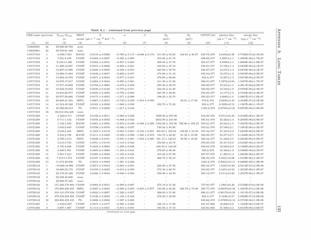
Appendix
A.
Long
Tables
135Table A.1 – continued from previous page
GRB name spectrum Tstart:Tstop BEST A α β Ep Eb CSTAT/dof photon flux energy flux
(s) model (ph s−1 cm−2 keV−1) (keV) (keV) (ph s−1 cm−2) (erg s−1 cm−2)
(1) (2) (3) (4) (5) (6) (7) (8) (9) (10) (11) (12)
110625881 42 29.906:38.793 none - - - - - - - -
110625881 43 38.793:61.440 none - - - - - - - -
110717319 1 -4.096:7.051 BAND 0.0118± 0.0028 −0.760± 0.117 −2.048± 0.174 311.00± 63.80 162.85± 36.07 639.73/476 2.8109±0.36 5.7790E-07±6.1E-08
110717319 2 7.051:9.156 COMP 0.0462± 0.0097 −0.590± 0.083 - 253.90± 21.70 - 498.89/477 8.3897±1.1 1.4695E-06±1.7E-07
110717319 3 9.156:11.290 COMP 0.0302± 0.0051 −0.957± 0.063 - 368.00± 47.70 - 504.57/477 8.8498±1.1 1.6082E-06±1.6E-07
110717319 4 11.290:12.697 COMP 0.0515± 0.0080 −0.862± 0.061 - 349.60± 37.10 - 546.81/477 13.706±1.4 2.5830E-06±2.1E-07
110717319 5 12.697:13.986 COMP 0.0406± 0.0056 −0.946± 0.055 - 465.90± 59.70 - 536.27/477 12.675±1.3 2.6270E-06±2.1E-07
110717319 6 13.986:15.084 COMP 0.0440± 0.0057 −0.800± 0.057 - 474.80± 51.10 - 559.24/477 12.575±1.2 2.9553E-06±2.2E-07
110717319 7 15.084:16.078 COMP 0.0471± 0.0054 −0.877± 0.051 - 576.60± 68.80 - 534.5/477 15.007±1.3 3.6474E-06±2.5E-07
110717319 8 16.078:17.817 COMP 0.0264± 0.0044 −0.885± 0.061 - 411.30± 51.20 - 488.91/477 7.5872±0.94 1.5457E-06±1.7E-07
110717319 9 17.817:18.602 COMP 0.0703± 0.0085 −0.679± 0.058 - 439.40± 38.70 - 529.08/477 18.215±1.5 4.4611E-06±2.9E-07
110717319 10 18.602:19.853 COMP 0.0630± 0.0128 −0.779± 0.071 - 244.40± 21.40 - 529.92/477 13.316±1.9 2.0750E-06±2.5E-07
110717319 11 19.853:20.977 COMP 0.0593± 0.0094 −0.759± 0.063 - 327.90± 29.80 - 576.23/477 14.177±1.5 2.7349E-06±2.4E-07
110717319 12 20.977:29.680 COMP 0.0175± 0.0055 −1.071± 0.089 - 188.20± 24.70 - 594.25/477 4.6082±1.0 5.2807E-07±1.0E-07
110717319 13 29.680:41.524 SBPL 0.0067± 0.0013 −0.740± 0.236 −1.810± 0.095 - 58.01± 17.90 576.8/476 2.6236±0.45 4.4546E-07±6.5E-08
110717319 14 41.524:45.569 COMP 0.0181± 0.0030 −1.080± 0.059 - 452.70± 75.50 - 550.4/477 6.2209±0.74 1.1367E-06±1.1E-07
110717319 15 45.569:88.612 PL 0.0011± 0.0003 −1.617± 0.045 - - - 1156.2/478 0.67934±0.21 9.0078E-08±2.6E-08
110717319 16 88.612:104.448 none - - - - - - - -
110721200 1 -1.024:0.711 COMP 0.0198± 0.0011 −0.980± 0.020 - 7409.00± 597.00 - 554.56/478 8.8715±0.50 3.0120E-06±1.3E-07
110721200 2 0.711:1.132 COMP 0.0556± 0.0034 −0.889± 0.024 - 2632.00± 216.00 - 585.61/478 23.424±1.4 8.2636E-06±4.0E-07
110721200 3 1.132:1.633 BAND 0.0601± 0.0050 −0.834± 0.036 −2.388± 0.206 1182.00± 165.00 782.80± 138.22 550.21/477 22.521±1.5 7.3227E-06±3.9E-07
110721200 4 1.633:2.043 COMP 0.0788± 0.0076 −0.926± 0.037 - 749.40± 85.90 - 533.31/478 27.548±2.1 7.1061E-06±4.5E-07
110721200 5 2.043:2.434 SBPL 0.1219± 0.0118 −0.662± 0.067 −2.104± 0.091 305.63± 102.84 130.80± 16.30 537.44/477 37.445±3.2 7.9245E-06±5.6E-07
110721200 6 2.434:2.798 BAND 0.2111± 0.0422 −0.588± 0.098 −1.925± 0.078 184.70± 23.00 91.30± 10.98 508.08/477 33.377±3.7 6.1246E-06±5.7E-07
110721200 7 2.798:3.213 SBPL 0.0826± 0.0101 −0.947± 0.081 −1.933± 0.085 331.13± 120.61 93.68± 18.00 530.44/477 31.348±3.5 5.2842E-06±5.0E-07
110721200 8 3.213:3.745 COMP 0.0761± 0.0119 −1.118± 0.044 - 354.00± 42.70 - 476.65/478 25.417±3.0 4.0182E-06±4.1E-07
110721200 9 3.745:4.430 COMP 0.0434± 0.0064 −1.299± 0.039 - 640.50± 144.00 - 458.65/478 18.940±2.3 3.1388E-06±3.2E-07
110721200 10 4.430:5.561 COMP 0.0403± 0.0060 −1.256± 0.041 - 479.60± 86.40 - 528.2/478 16.302±1.9 2.5908E-06±2.5E-07
110721200 11 5.561:7.413 COMP 0.0305± 0.0049 −1.183± 0.045 - 419.20± 67.30 - 587.07/478 11.265±1.4 1.8202E-06±1.8E-07
110721200 12 7.413:11.074 COMP 0.0187± 0.0034 −1.128± 0.051 - 366.70± 56.10 - 596.45/478 6.3621±0.88 1.0149E-06±1.2E-07
110721200 13 11.074:39.936 PL 0.0010± 0.0002 −1.381± 0.026 - - - 1349.2/479 0.50612±0.11 9.8288E-08±1.9E-08
110729142 1 -19.808:18.080 COMP 0.0074± 0.0019 −0.804± 0.081 - 248.90± 27.90 - 683.33/477 1.6165±0.29 2.5214E-07±3.9E-08
110729142 2 18.080:22.176 COMP 0.0165± 0.0022 −0.913± 0.050 - 572.40± 80.70 - 550.82/477 5.3451±0.53 1.2552E-06±1.0E-07
110729142 3 22.176:25.248 COMP 0.0246± 0.0044 −0.848± 0.063 - 356.90± 42.30 - 503.12/477 6.5114±0.82 1.2547E-06±1.3E-07
110729142 4 25.248:40.609 none - - - - - - - -
110729142 5 40.609:75.425 none - - - - - - - -
110729142 6 151.202:176.803 COMP 0.0064± 0.0015 −0.899± 0.067 - 274.10± 31.20 - 737.05/477 1.5881±0.30 2.5120E-07±4.4E-08
110729142 7 176.803:200.355 SBPL 0.0027± 0.0010 −0.998± 0.085 −2.845± 0.877 193.89± 92.28 186.70± 74.00 585.77/476 0.95079±0.36 1.4367E-07±4.9E-08
110729142 8 319.141:379.558 COMP 0.0024± 0.0007 −1.226± 0.057 - 298.00± 51.90 - 890.21/477 0.86170±0.23 1.1611E-07±2.9E-08
110729142 9 379.558:393.894 COMP 0.0126± 0.0023 −1.160± 0.049 - 276.20± 33.90 - 562.4/477 4.1238±0.57 5.5992E-07±6.6E-08
110729142 10 393.894:459.431 PL 0.0008± 0.0002 −1.597± 0.025 - - - 839.68/478 0.47959±0.14 6.5753E-08±1.9E-08
110731465 1 -1.024:0.897 COMP 0.0475± 0.0177 −0.985± 0.093 - 164.10± 17.90 - 401.07/360 10.608±3.0 1.1549E-06±3.0E-07
110731465 2 0.897:1.807 COMP 0.1114± 0.0331 −0.815± 0.091 - 183.00± 17.10 - 423.65/360 21.220±4.2 2.6510E-06±4.6E-07
Continued on next page
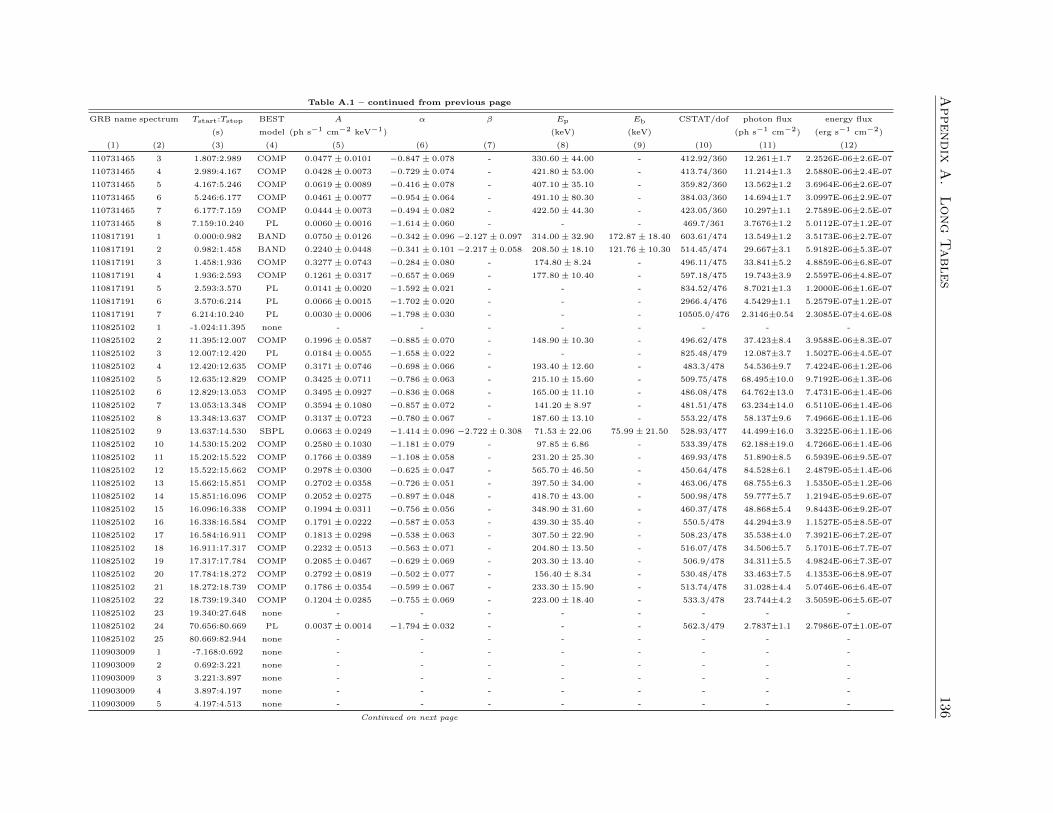
Appendix
A.
Long
Tables
136Table A.1 – continued from previous page
GRB name spectrum Tstart:Tstop BEST A α β Ep Eb CSTAT/dof photon flux energy flux
(s) model (ph s−1 cm−2 keV−1) (keV) (keV) (ph s−1 cm−2) (erg s−1 cm−2)
(1) (2) (3) (4) (5) (6) (7) (8) (9) (10) (11) (12)
110731465 3 1.807:2.989 COMP 0.0477± 0.0101 −0.847± 0.078 - 330.60± 44.00 - 412.92/360 12.261±1.7 2.2526E-06±2.6E-07
110731465 4 2.989:4.167 COMP 0.0428± 0.0073 −0.729± 0.074 - 421.80± 53.00 - 413.74/360 11.214±1.3 2.5880E-06±2.4E-07
110731465 5 4.167:5.246 COMP 0.0619± 0.0089 −0.416± 0.078 - 407.10± 35.10 - 359.82/360 13.562±1.2 3.6964E-06±2.6E-07
110731465 6 5.246:6.177 COMP 0.0461± 0.0077 −0.954± 0.064 - 491.10± 80.30 - 384.03/360 14.694±1.7 3.0997E-06±2.9E-07
110731465 7 6.177:7.159 COMP 0.0444± 0.0073 −0.494± 0.082 - 422.50± 44.30 - 423.05/360 10.297±1.1 2.7589E-06±2.5E-07
110731465 8 7.159:10.240 PL 0.0060± 0.0016 −1.614± 0.060 - - - 469.7/361 3.7676±1.2 5.0112E-07±1.2E-07
110817191 1 0.000:0.982 BAND 0.0750± 0.0126 −0.342± 0.096 −2.127± 0.097 314.00± 32.90 172.87± 18.40 603.61/474 13.549±1.2 3.5173E-06±2.7E-07
110817191 2 0.982:1.458 BAND 0.2240± 0.0448 −0.341± 0.101 −2.217± 0.058 208.50± 18.10 121.76± 10.30 514.45/474 29.667±3.1 5.9182E-06±5.3E-07
110817191 3 1.458:1.936 COMP 0.3277± 0.0743 −0.284± 0.080 - 174.80± 8.24 - 496.11/475 33.841±5.2 4.8859E-06±6.8E-07
110817191 4 1.936:2.593 COMP 0.1261± 0.0317 −0.657± 0.069 - 177.80± 10.40 - 597.18/475 19.743±3.9 2.5597E-06±4.8E-07
110817191 5 2.593:3.570 PL 0.0141± 0.0020 −1.592± 0.021 - - - 834.52/476 8.7021±1.3 1.2000E-06±1.6E-07
110817191 6 3.570:6.214 PL 0.0066± 0.0015 −1.702± 0.020 - - - 2966.4/476 4.5429±1.1 5.2579E-07±1.2E-07
110817191 7 6.214:10.240 PL 0.0030± 0.0006 −1.798± 0.030 - - - 10505.0/476 2.3146±0.54 2.3085E-07±4.6E-08
110825102 1 -1.024:11.395 none - - - - - - - -
110825102 2 11.395:12.007 COMP 0.1996± 0.0587 −0.885± 0.070 - 148.90± 10.30 - 496.62/478 37.423±8.4 3.9588E-06±8.3E-07
110825102 3 12.007:12.420 PL 0.0184± 0.0055 −1.658± 0.022 - - - 825.48/479 12.087±3.7 1.5027E-06±4.5E-07
110825102 4 12.420:12.635 COMP 0.3171± 0.0746 −0.698± 0.066 - 193.40± 12.60 - 483.3/478 54.536±9.7 7.4224E-06±1.2E-06
110825102 5 12.635:12.829 COMP 0.3425± 0.0711 −0.786± 0.063 - 215.10± 15.60 - 509.75/478 68.495±10.0 9.7192E-06±1.3E-06
110825102 6 12.829:13.053 COMP 0.3495± 0.0927 −0.836± 0.068 - 165.00± 11.10 - 486.08/478 64.762±13.0 7.4731E-06±1.4E-06
110825102 7 13.053:13.348 COMP 0.3594± 0.1080 −0.857± 0.072 - 141.20± 8.97 - 481.51/478 63.234±14.0 6.5110E-06±1.4E-06
110825102 8 13.348:13.637 COMP 0.3137± 0.0723 −0.780± 0.067 - 187.60± 13.10 - 553.22/478 58.137±9.6 7.4966E-06±1.1E-06
110825102 9 13.637:14.530 SBPL 0.0663± 0.0249 −1.414± 0.096 −2.722± 0.308 71.53± 22.06 75.99± 21.50 528.93/477 44.499±16.0 3.3225E-06±1.1E-06
110825102 10 14.530:15.202 COMP 0.2580± 0.1030 −1.181± 0.079 - 97.85± 6.86 - 533.39/478 62.188±19.0 4.7266E-06±1.4E-06
110825102 11 15.202:15.522 COMP 0.1766± 0.0389 −1.108± 0.058 - 231.20± 25.30 - 469.93/478 51.890±8.5 6.5939E-06±9.5E-07
110825102 12 15.522:15.662 COMP 0.2978± 0.0300 −0.625± 0.047 - 565.70± 46.50 - 450.64/478 84.528±6.1 2.4879E-05±1.4E-06
110825102 13 15.662:15.851 COMP 0.2702± 0.0358 −0.726± 0.051 - 397.50± 34.00 - 463.06/478 68.755±6.3 1.5350E-05±1.2E-06
110825102 14 15.851:16.096 COMP 0.2052± 0.0275 −0.897± 0.048 - 418.70± 43.00 - 500.98/478 59.777±5.7 1.2194E-05±9.6E-07
110825102 15 16.096:16.338 COMP 0.1994± 0.0311 −0.756± 0.056 - 348.90± 31.60 - 460.37/478 48.868±5.4 9.8443E-06±9.2E-07
110825102 16 16.338:16.584 COMP 0.1791± 0.0222 −0.587± 0.053 - 439.30± 35.40 - 550.5/478 44.294±3.9 1.1527E-05±8.5E-07
110825102 17 16.584:16.911 COMP 0.1813± 0.0298 −0.538± 0.063 - 307.50± 22.90 - 508.23/478 35.538±4.0 7.3921E-06±7.2E-07
110825102 18 16.911:17.317 COMP 0.2232± 0.0513 −0.563± 0.071 - 204.80± 13.50 - 516.07/478 34.506±5.7 5.1701E-06±7.7E-07
110825102 19 17.317:17.784 COMP 0.2085± 0.0467 −0.629± 0.069 - 203.30± 13.40 - 506.9/478 34.311±5.5 4.9824E-06±7.3E-07
110825102 20 17.784:18.272 COMP 0.2792± 0.0819 −0.502± 0.077 - 156.40± 8.34 - 530.48/478 33.463±7.5 4.1353E-06±8.9E-07
110825102 21 18.272:18.739 COMP 0.1786± 0.0354 −0.599± 0.067 - 233.30± 15.90 - 513.74/478 31.028±4.4 5.0746E-06±6.4E-07
110825102 22 18.739:19.340 COMP 0.1204± 0.0285 −0.755± 0.069 - 223.00± 18.40 - 533.3/478 23.744±4.2 3.5059E-06±5.6E-07
110825102 23 19.340:27.648 none - - - - - - - -
110825102 24 70.656:80.669 PL 0.0037± 0.0014 −1.794± 0.032 - - - 562.3/479 2.7837±1.1 2.7986E-07±1.0E-07
110825102 25 80.669:82.944 none - - - - - - - -
110903009 1 -7.168:0.692 none - - - - - - - -
110903009 2 0.692:3.221 none - - - - - - - -
110903009 3 3.221:3.897 none - - - - - - - -
110903009 4 3.897:4.197 none - - - - - - - -
110903009 5 4.197:4.513 none - - - - - - - -
Continued on next page
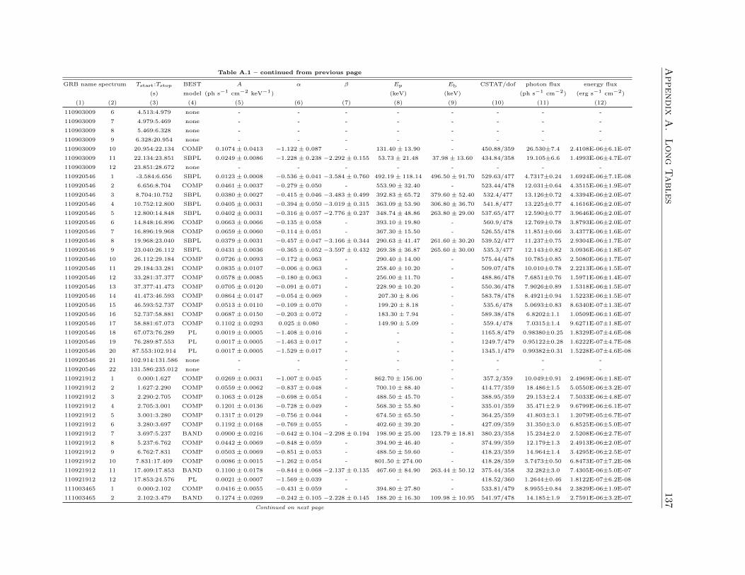
Appendix
A.
Long
Tables
137Table A.1 – continued from previous page
GRB name spectrum Tstart:Tstop BEST A α β Ep Eb CSTAT/dof photon flux energy flux
(s) model (ph s−1 cm−2 keV−1) (keV) (keV) (ph s−1 cm−2) (erg s−1 cm−2)
(1) (2) (3) (4) (5) (6) (7) (8) (9) (10) (11) (12)
110903009 6 4.513:4.979 none - - - - - - - -
110903009 7 4.979:5.469 none - - - - - - - -
110903009 8 5.469:6.328 none - - - - - - - -
110903009 9 6.328:20.954 none - - - - - - - -
110903009 10 20.954:22.134 COMP 0.1074± 0.0413 −1.122± 0.087 - 131.40± 13.90 - 450.88/359 26.530±7.4 2.4108E-06±6.1E-07
110903009 11 22.134:23.851 SBPL 0.0249± 0.0086 −1.228± 0.238 −2.292± 0.155 53.73± 21.48 37.98± 13.60 434.84/358 19.105±6.6 1.4993E-06±4.7E-07
110903009 12 23.851:28.672 none - - - - - - - -
110920546 1 -3.584:6.656 SBPL 0.0123± 0.0008 −0.536± 0.041 −3.584± 0.760 492.19± 118.14 496.50± 91.70 529.63/477 4.7317±0.24 1.6924E-06±7.1E-08
110920546 2 6.656:8.704 COMP 0.0461± 0.0037 −0.279± 0.050 - 553.90± 32.40 - 523.44/478 12.031±0.64 4.3515E-06±1.9E-07
110920546 3 8.704:10.752 SBPL 0.0380± 0.0027 −0.415± 0.046 −3.483± 0.499 392.83± 65.72 379.60± 52.40 532.4/477 13.126±0.72 4.3394E-06±2.0E-07
110920546 4 10.752:12.800 SBPL 0.0405± 0.0031 −0.394± 0.050 −3.019± 0.315 363.09± 53.90 306.80± 36.70 541.8/477 13.225±0.77 4.1616E-06±2.0E-07
110920546 5 12.800:14.848 SBPL 0.0402± 0.0031 −0.316± 0.057 −2.776± 0.237 348.74± 48.86 263.80± 29.00 537.65/477 12.590±0.77 3.9646E-06±2.0E-07
110920546 6 14.848:16.896 COMP 0.0663± 0.0066 −0.135± 0.058 - 393.10± 19.80 - 560.9/478 12.769±0.78 3.8793E-06±2.0E-07
110920546 7 16.896:19.968 COMP 0.0659± 0.0060 −0.114± 0.051 - 367.30± 15.50 - 526.55/478 11.851±0.66 3.4377E-06±1.6E-07
110920546 8 19.968:23.040 SBPL 0.0379± 0.0031 −0.457± 0.047 −3.166± 0.344 290.63± 41.47 261.60± 30.20 539.52/477 11.237±0.75 2.9304E-06±1.7E-07
110920546 9 23.040:26.112 SBPL 0.0431± 0.0036 −0.365± 0.052 −3.597± 0.432 269.38± 36.87 265.60± 30.00 535.3/477 12.143±0.82 3.0936E-06±1.8E-07
110920546 10 26.112:29.184 COMP 0.0726± 0.0093 −0.172± 0.063 - 290.40± 14.00 - 575.44/478 10.785±0.85 2.5080E-06±1.7E-07
110920546 11 29.184:33.281 COMP 0.0835± 0.0107 −0.006± 0.063 - 258.40± 10.20 - 509.07/478 10.010±0.78 2.2213E-06±1.5E-07
110920546 12 33.281:37.377 COMP 0.0578± 0.0085 −0.180± 0.063 - 256.00± 11.70 - 488.86/478 7.6851±0.76 1.5971E-06±1.4E-07
110920546 13 37.377:41.473 COMP 0.0705± 0.0120 −0.091± 0.071 - 228.90± 10.20 - 550.36/478 7.9026±0.89 1.5318E-06±1.5E-07
110920546 14 41.473:46.593 COMP 0.0864± 0.0147 −0.054± 0.069 - 207.30± 8.06 - 583.78/478 8.4921±0.94 1.5223E-06±1.5E-07
110920546 15 46.593:52.737 COMP 0.0513± 0.0110 −0.109± 0.070 - 199.20± 8.18 - 535.6/478 5.0693±0.83 8.6340E-07±1.3E-07
110920546 16 52.737:58.881 COMP 0.0687± 0.0150 −0.203± 0.072 - 183.30± 7.94 - 589.38/478 6.8202±1.1 1.0509E-06±1.6E-07
110920546 17 58.881:67.073 COMP 0.1102± 0.0293 0.025± 0.080 - 149.90± 5.09 - 559.4/478 7.0315±1.4 9.6271E-07±1.8E-07
110920546 18 67.073:76.289 PL 0.0019± 0.0005 −1.408± 0.016 - - - 1165.8/479 0.98380±0.25 1.8329E-07±4.6E-08
110920546 19 76.289:87.553 PL 0.0017± 0.0005 −1.463± 0.017 - - - 1249.7/479 0.95122±0.28 1.6222E-07±4.7E-08
110920546 20 87.553:102.914 PL 0.0017± 0.0005 −1.529± 0.017 - - - 1345.1/479 0.99382±0.31 1.5228E-07±4.6E-08
110920546 21 102.914:131.586 none - - - - - - - -
110920546 22 131.586:235.012 none - - - - - - - -
110921912 1 0.000:1.627 COMP 0.0269± 0.0031 −1.007± 0.045 - 862.70± 156.00 - 357.2/359 10.049±0.91 2.4969E-06±1.8E-07
110921912 2 1.627:2.290 COMP 0.0559± 0.0062 −0.837± 0.048 - 700.10± 88.40 - 414.77/359 18.486±1.5 5.0550E-06±3.2E-07
110921912 3 2.290:2.705 COMP 0.1063± 0.0128 −0.698± 0.054 - 488.50± 45.70 - 388.95/359 29.153±2.4 7.5033E-06±4.8E-07
110921912 4 2.705:3.001 COMP 0.1201± 0.0136 −0.728± 0.049 - 568.30± 55.80 - 335.01/359 35.471±2.9 9.6799E-06±6.1E-07
110921912 5 3.001:3.280 COMP 0.1317± 0.0129 −0.756± 0.044 - 674.50± 65.50 - 364.25/359 41.803±3.1 1.2079E-05±6.7E-07
110921912 6 3.280:3.697 COMP 0.1192± 0.0168 −0.769± 0.055 - 402.60± 39.20 - 427.09/359 31.350±3.0 6.8525E-06±5.0E-07
110921912 7 3.697:5.237 BAND 0.0900± 0.0216 −0.642± 0.104 −2.298± 0.194 198.90± 25.00 123.79± 18.81 380.23/358 15.234±2.0 2.5208E-06±2.7E-07
110921912 8 5.237:6.762 COMP 0.0442± 0.0069 −0.848± 0.059 - 394.90± 46.40 - 374.99/359 12.179±1.3 2.4913E-06±2.0E-07
110921912 9 6.762:7.831 COMP 0.0503± 0.0069 −0.851± 0.053 - 488.50± 59.60 - 418.23/359 14.964±1.4 3.4295E-06±2.5E-07
110921912 10 7.831:17.409 COMP 0.0086± 0.0015 −1.262± 0.054 - 801.50± 274.00 - 418.28/359 3.7473±0.50 6.8473E-07±7.2E-08
110921912 11 17.409:17.853 BAND 0.1100± 0.0178 −0.844± 0.068 −2.137± 0.135 467.60± 84.90 263.44± 50.12 375.44/358 32.282±3.0 7.4305E-06±5.0E-07
110921912 12 17.853:24.576 PL 0.0021± 0.0007 −1.569± 0.039 - - - 418.52/360 1.2644±0.46 1.8122E-07±6.2E-08
111003465 1 0.000:2.102 COMP 0.0416± 0.0055 −0.431± 0.059 - 394.80± 27.80 - 533.81/479 8.9955±0.84 2.3829E-06±1.9E-07
111003465 2 2.102:3.479 BAND 0.1274± 0.0269 −0.242± 0.105 −2.228± 0.145 188.20± 16.30 109.98± 10.95 541.97/478 14.185±1.9 2.7591E-06±3.2E-07
Continued on next page
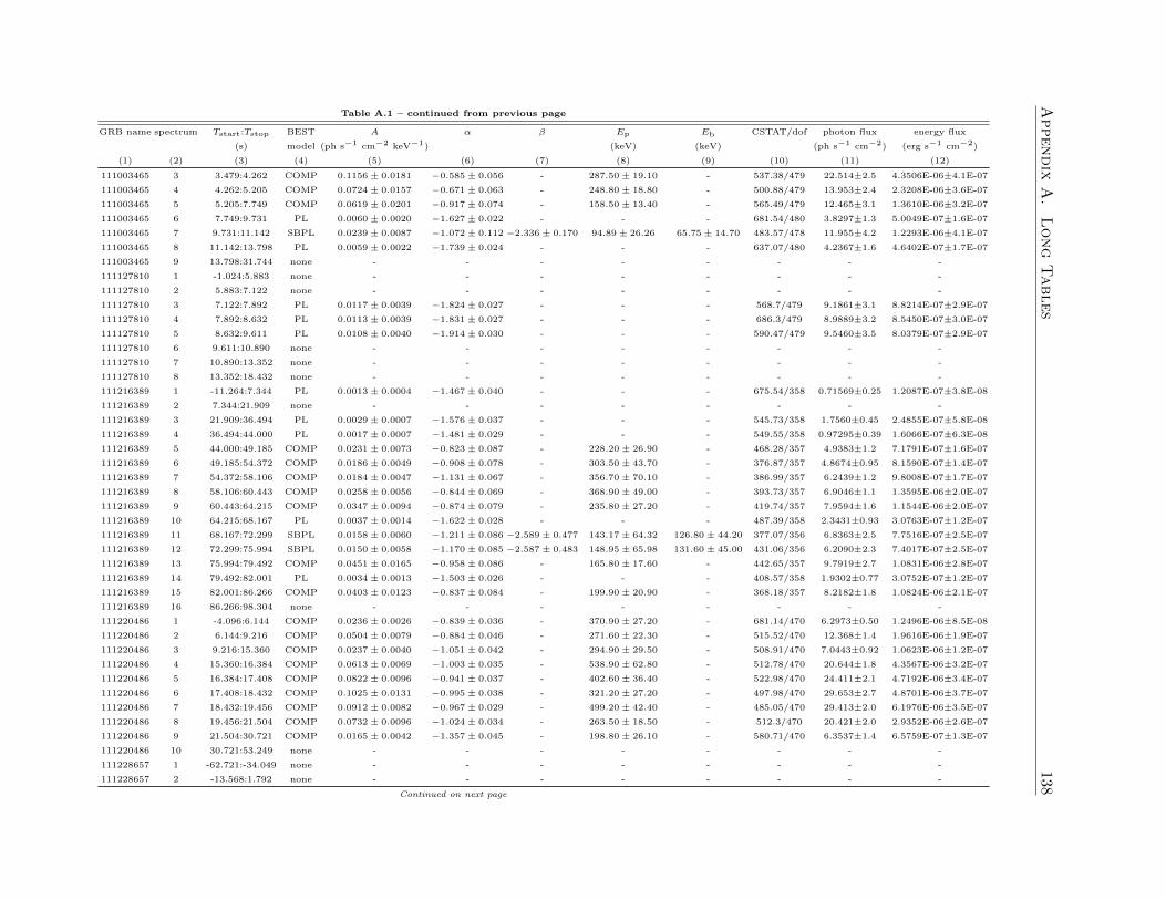
Appendix
A.
Long
Tables
138Table A.1 – continued from previous page
GRB name spectrum Tstart:Tstop BEST A α β Ep Eb CSTAT/dof photon flux energy flux
(s) model (ph s−1 cm−2 keV−1) (keV) (keV) (ph s−1 cm−2) (erg s−1 cm−2)
(1) (2) (3) (4) (5) (6) (7) (8) (9) (10) (11) (12)
111003465 3 3.479:4.262 COMP 0.1156± 0.0181 −0.585± 0.056 - 287.50± 19.10 - 537.38/479 22.514±2.5 4.3506E-06±4.1E-07
111003465 4 4.262:5.205 COMP 0.0724± 0.0157 −0.671± 0.063 - 248.80± 18.80 - 500.88/479 13.953±2.4 2.3208E-06±3.6E-07
111003465 5 5.205:7.749 COMP 0.0619± 0.0201 −0.917± 0.074 - 158.50± 13.40 - 565.49/479 12.465±3.1 1.3610E-06±3.2E-07
111003465 6 7.749:9.731 PL 0.0060± 0.0020 −1.627± 0.022 - - - 681.54/480 3.8297±1.3 5.0049E-07±1.6E-07
111003465 7 9.731:11.142 SBPL 0.0239± 0.0087 −1.072± 0.112 −2.336± 0.170 94.89± 26.26 65.75± 14.70 483.57/478 11.955±4.2 1.2293E-06±4.1E-07
111003465 8 11.142:13.798 PL 0.0059± 0.0022 −1.739± 0.024 - - - 637.07/480 4.2367±1.6 4.6402E-07±1.7E-07
111003465 9 13.798:31.744 none - - - - - - - -
111127810 1 -1.024:5.883 none - - - - - - - -
111127810 2 5.883:7.122 none - - - - - - - -
111127810 3 7.122:7.892 PL 0.0117± 0.0039 −1.824± 0.027 - - - 568.7/479 9.1861±3.1 8.8214E-07±2.9E-07
111127810 4 7.892:8.632 PL 0.0113± 0.0039 −1.831± 0.027 - - - 686.3/479 8.9889±3.2 8.5450E-07±3.0E-07
111127810 5 8.632:9.611 PL 0.0108± 0.0040 −1.914± 0.030 - - - 590.47/479 9.5460±3.5 8.0379E-07±2.9E-07
111127810 6 9.611:10.890 none - - - - - - - -
111127810 7 10.890:13.352 none - - - - - - - -
111127810 8 13.352:18.432 none - - - - - - - -
111216389 1 -11.264:7.344 PL 0.0013± 0.0004 −1.467± 0.040 - - - 675.54/358 0.71569±0.25 1.2087E-07±3.8E-08
111216389 2 7.344:21.909 none - - - - - - - -
111216389 3 21.909:36.494 PL 0.0029± 0.0007 −1.576± 0.037 - - - 545.73/358 1.7560±0.45 2.4855E-07±5.8E-08
111216389 4 36.494:44.000 PL 0.0017± 0.0007 −1.481± 0.029 - - - 549.55/358 0.97295±0.39 1.6066E-07±6.3E-08
111216389 5 44.000:49.185 COMP 0.0231± 0.0073 −0.823± 0.087 - 228.20± 26.90 - 468.28/357 4.9383±1.2 7.1791E-07±1.6E-07
111216389 6 49.185:54.372 COMP 0.0186± 0.0049 −0.908± 0.078 - 303.50± 43.70 - 376.87/357 4.8674±0.95 8.1590E-07±1.4E-07
111216389 7 54.372:58.106 COMP 0.0184± 0.0047 −1.131± 0.067 - 356.70± 70.10 - 386.99/357 6.2439±1.2 9.8008E-07±1.7E-07
111216389 8 58.106:60.443 COMP 0.0258± 0.0056 −0.844± 0.069 - 368.90± 49.00 - 393.73/357 6.9046±1.1 1.3595E-06±2.0E-07
111216389 9 60.443:64.215 COMP 0.0347± 0.0094 −0.874± 0.079 - 235.80± 27.20 - 419.74/357 7.9594±1.6 1.1544E-06±2.0E-07
111216389 10 64.215:68.167 PL 0.0037± 0.0014 −1.622± 0.028 - - - 487.39/358 2.3431±0.93 3.0763E-07±1.2E-07
111216389 11 68.167:72.299 SBPL 0.0158± 0.0060 −1.211± 0.086 −2.589± 0.477 143.17± 64.32 126.80± 44.20 377.07/356 6.8363±2.5 7.7516E-07±2.5E-07
111216389 12 72.299:75.994 SBPL 0.0150± 0.0058 −1.170± 0.085 −2.587± 0.483 148.95± 65.98 131.60± 45.00 431.06/356 6.2090±2.3 7.4017E-07±2.5E-07
111216389 13 75.994:79.492 COMP 0.0451± 0.0165 −0.958± 0.086 - 165.80± 17.60 - 442.65/357 9.7919±2.7 1.0831E-06±2.8E-07
111216389 14 79.492:82.001 PL 0.0034± 0.0013 −1.503± 0.026 - - - 408.57/358 1.9302±0.77 3.0752E-07±1.2E-07
111216389 15 82.001:86.266 COMP 0.0403± 0.0123 −0.837± 0.084 - 199.90± 20.90 - 368.18/357 8.2182±1.8 1.0824E-06±2.1E-07
111216389 16 86.266:98.304 none - - - - - - - -
111220486 1 -4.096:6.144 COMP 0.0236± 0.0026 −0.839± 0.036 - 370.90± 27.20 - 681.14/470 6.2973±0.50 1.2496E-06±8.5E-08
111220486 2 6.144:9.216 COMP 0.0504± 0.0079 −0.884± 0.046 - 271.60± 22.30 - 515.52/470 12.368±1.4 1.9616E-06±1.9E-07
111220486 3 9.216:15.360 COMP 0.0237± 0.0040 −1.051± 0.042 - 294.90± 29.50 - 508.91/470 7.0443±0.92 1.0623E-06±1.2E-07
111220486 4 15.360:16.384 COMP 0.0613± 0.0069 −1.003± 0.035 - 538.90± 62.80 - 512.78/470 20.644±1.8 4.3567E-06±3.2E-07
111220486 5 16.384:17.408 COMP 0.0822± 0.0096 −0.941± 0.037 - 402.60± 36.40 - 522.98/470 24.411±2.1 4.7192E-06±3.4E-07
111220486 6 17.408:18.432 COMP 0.1025± 0.0131 −0.995± 0.038 - 321.20± 27.20 - 497.98/470 29.653±2.7 4.8701E-06±3.7E-07
111220486 7 18.432:19.456 COMP 0.0912± 0.0082 −0.967± 0.029 - 499.20± 42.40 - 485.05/470 29.413±2.0 6.1976E-06±3.5E-07
111220486 8 19.456:21.504 COMP 0.0732± 0.0096 −1.024± 0.034 - 263.50± 18.50 - 512.3/470 20.421±2.0 2.9352E-06±2.6E-07
111220486 9 21.504:30.721 COMP 0.0165± 0.0042 −1.357± 0.045 - 198.80± 26.10 - 580.71/470 6.3537±1.4 6.5759E-07±1.3E-07
111220486 10 30.721:53.249 none - - - - - - - -
111228657 1 -62.721:-34.049 none - - - - - - - -
111228657 2 -13.568:1.792 none - - - - - - - -
Continued on next page
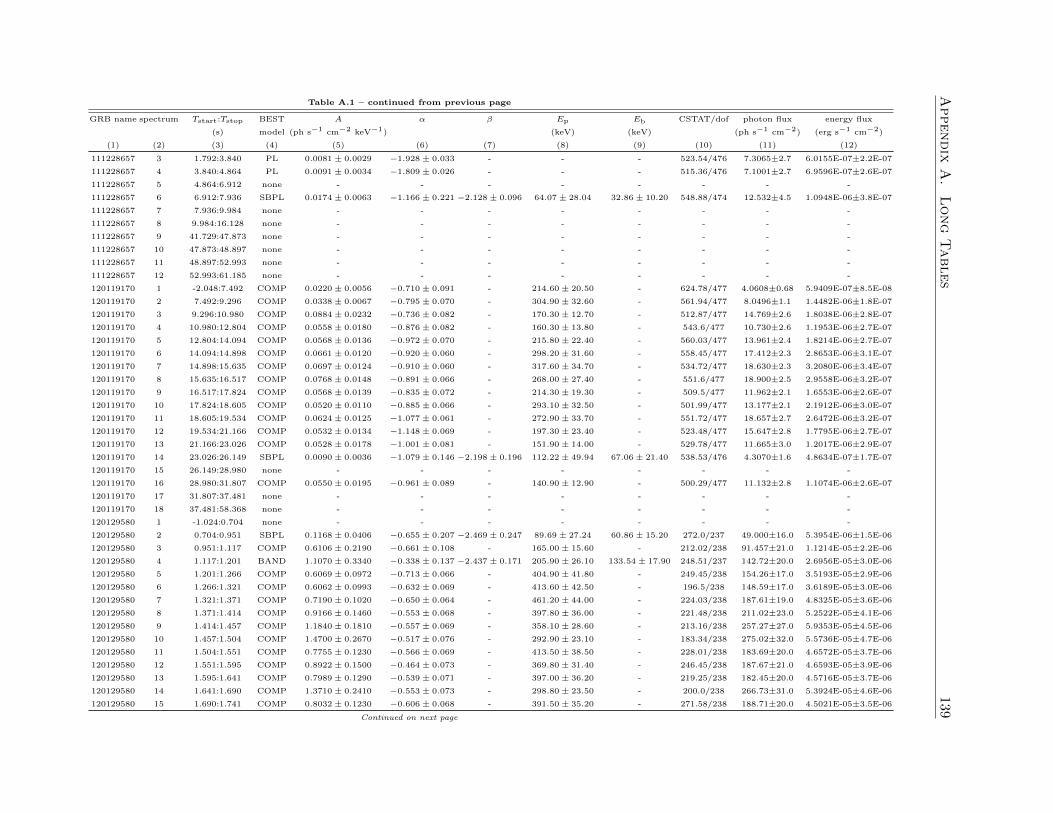
Appendix
A.
Long
Tables
139Table A.1 – continued from previous page
GRB name spectrum Tstart:Tstop BEST A α β Ep Eb CSTAT/dof photon flux energy flux
(s) model (ph s−1 cm−2 keV−1) (keV) (keV) (ph s−1 cm−2) (erg s−1 cm−2)
(1) (2) (3) (4) (5) (6) (7) (8) (9) (10) (11) (12)
111228657 3 1.792:3.840 PL 0.0081± 0.0029 −1.928± 0.033 - - - 523.54/476 7.3065±2.7 6.0155E-07±2.2E-07
111228657 4 3.840:4.864 PL 0.0091± 0.0034 −1.809± 0.026 - - - 515.36/476 7.1001±2.7 6.9596E-07±2.6E-07
111228657 5 4.864:6.912 none - - - - - - - -
111228657 6 6.912:7.936 SBPL 0.0174± 0.0063 −1.166± 0.221 −2.128± 0.096 64.07± 28.04 32.86± 10.20 548.88/474 12.532±4.5 1.0948E-06±3.8E-07
111228657 7 7.936:9.984 none - - - - - - - -
111228657 8 9.984:16.128 none - - - - - - - -
111228657 9 41.729:47.873 none - - - - - - - -
111228657 10 47.873:48.897 none - - - - - - - -
111228657 11 48.897:52.993 none - - - - - - - -
111228657 12 52.993:61.185 none - - - - - - - -
120119170 1 -2.048:7.492 COMP 0.0220± 0.0056 −0.710± 0.091 - 214.60± 20.50 - 624.78/477 4.0608±0.68 5.9409E-07±8.5E-08
120119170 2 7.492:9.296 COMP 0.0338± 0.0067 −0.795± 0.070 - 304.90± 32.60 - 561.94/477 8.0496±1.1 1.4482E-06±1.8E-07
120119170 3 9.296:10.980 COMP 0.0884± 0.0232 −0.736± 0.082 - 170.30± 12.70 - 512.87/477 14.769±2.6 1.8038E-06±2.8E-07
120119170 4 10.980:12.804 COMP 0.0558± 0.0180 −0.876± 0.082 - 160.30± 13.80 - 543.6/477 10.730±2.6 1.1953E-06±2.7E-07
120119170 5 12.804:14.094 COMP 0.0568± 0.0136 −0.972± 0.070 - 215.80± 22.40 - 560.03/477 13.961±2.4 1.8214E-06±2.7E-07
120119170 6 14.094:14.898 COMP 0.0661± 0.0120 −0.920± 0.060 - 298.20± 31.60 - 558.45/477 17.412±2.3 2.8653E-06±3.1E-07
120119170 7 14.898:15.635 COMP 0.0697± 0.0124 −0.910± 0.060 - 317.60± 34.70 - 534.72/477 18.630±2.3 3.2080E-06±3.4E-07
120119170 8 15.635:16.517 COMP 0.0768± 0.0148 −0.891± 0.066 - 268.00± 27.40 - 551.6/477 18.900±2.5 2.9558E-06±3.2E-07
120119170 9 16.517:17.824 COMP 0.0568± 0.0139 −0.835± 0.072 - 214.30± 19.30 - 509.5/477 11.962±2.1 1.6553E-06±2.6E-07
120119170 10 17.824:18.605 COMP 0.0520± 0.0110 −0.885± 0.066 - 293.10± 32.50 - 501.99/477 13.177±2.1 2.1912E-06±3.0E-07
120119170 11 18.605:19.534 COMP 0.0624± 0.0125 −1.077± 0.061 - 272.90± 33.70 - 551.72/477 18.657±2.7 2.6472E-06±3.2E-07
120119170 12 19.534:21.166 COMP 0.0532± 0.0134 −1.148± 0.069 - 197.30± 23.40 - 523.48/477 15.647±2.8 1.7795E-06±2.7E-07
120119170 13 21.166:23.026 COMP 0.0528± 0.0178 −1.001± 0.081 - 151.90± 14.00 - 529.78/477 11.665±3.0 1.2017E-06±2.9E-07
120119170 14 23.026:26.149 SBPL 0.0090± 0.0036 −1.079± 0.146 −2.198± 0.196 112.22± 49.94 67.06± 21.40 538.53/476 4.3070±1.6 4.8634E-07±1.7E-07
120119170 15 26.149:28.980 none - - - - - - - -
120119170 16 28.980:31.807 COMP 0.0550± 0.0195 −0.961± 0.089 - 140.90± 12.90 - 500.29/477 11.132±2.8 1.1074E-06±2.6E-07
120119170 17 31.807:37.481 none - - - - - - - -
120119170 18 37.481:58.368 none - - - - - - - -
120129580 1 -1.024:0.704 none - - - - - - - -
120129580 2 0.704:0.951 SBPL 0.1168± 0.0406 −0.655± 0.207 −2.469± 0.247 89.69± 27.24 60.86± 15.20 272.0/237 49.000±16.0 5.3954E-06±1.5E-06
120129580 3 0.951:1.117 COMP 0.6106± 0.2190 −0.661± 0.108 - 165.00± 15.60 - 212.02/238 91.457±21.0 1.1214E-05±2.2E-06
120129580 4 1.117:1.201 BAND 1.1070± 0.3340 −0.338± 0.137 −2.437± 0.171 205.90± 26.10 133.54± 17.90 248.51/237 142.72±20.0 2.6956E-05±3.0E-06
120129580 5 1.201:1.266 COMP 0.6069± 0.0972 −0.713± 0.066 - 404.90± 41.80 - 249.45/238 154.26±17.0 3.5193E-05±2.9E-06
120129580 6 1.266:1.321 COMP 0.6062± 0.0993 −0.632± 0.069 - 413.60± 42.50 - 196.5/238 148.59±17.0 3.6189E-05±3.0E-06
120129580 7 1.321:1.371 COMP 0.7190± 0.1020 −0.650± 0.064 - 461.20± 44.00 - 224.03/238 187.61±19.0 4.8325E-05±3.6E-06
120129580 8 1.371:1.414 COMP 0.9166± 0.1460 −0.553± 0.068 - 397.80± 36.00 - 221.48/238 211.02±23.0 5.2522E-05±4.1E-06
120129580 9 1.414:1.457 COMP 1.1840± 0.1810 −0.557± 0.069 - 358.10± 28.60 - 213.16/238 257.27±27.0 5.9353E-05±4.5E-06
120129580 10 1.457:1.504 COMP 1.4700± 0.2670 −0.517± 0.076 - 292.90± 23.10 - 183.34/238 275.02±32.0 5.5736E-05±4.7E-06
120129580 11 1.504:1.551 COMP 0.7755± 0.1230 −0.566± 0.069 - 413.50± 38.50 - 228.01/238 183.69±20.0 4.6572E-05±3.7E-06
120129580 12 1.551:1.595 COMP 0.8922± 0.1500 −0.464± 0.073 - 369.80± 31.40 - 246.45/238 187.67±21.0 4.6593E-05±3.9E-06
120129580 13 1.595:1.641 COMP 0.7989± 0.1290 −0.539± 0.071 - 397.00± 36.20 - 219.25/238 182.45±20.0 4.5716E-05±3.7E-06
120129580 14 1.641:1.690 COMP 1.3710± 0.2410 −0.553± 0.073 - 298.80± 23.50 - 200.0/238 266.73±31.0 5.3924E-05±4.6E-06
120129580 15 1.690:1.741 COMP 0.8032± 0.1230 −0.606± 0.068 - 391.50± 35.20 - 271.58/238 188.71±20.0 4.5021E-05±3.5E-06
Continued on next page
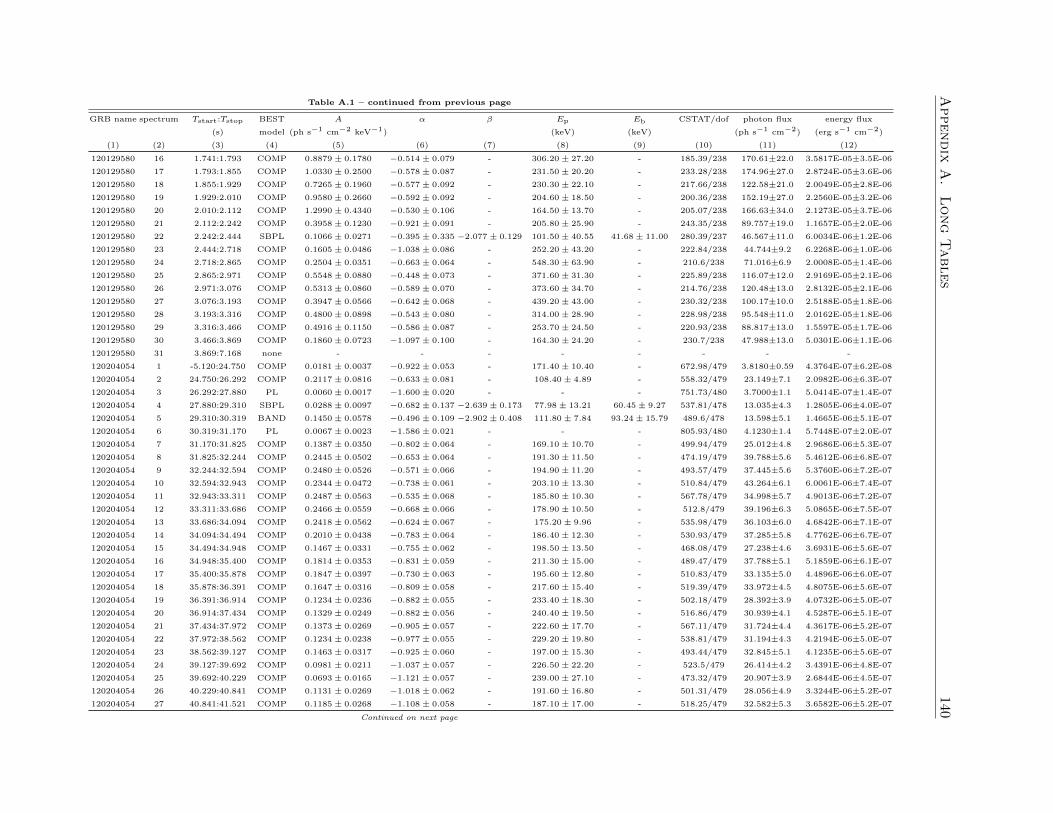
Appendix
A.
Long
Tables
140Table A.1 – continued from previous page
GRB name spectrum Tstart:Tstop BEST A α β Ep Eb CSTAT/dof photon flux energy flux
(s) model (ph s−1 cm−2 keV−1) (keV) (keV) (ph s−1 cm−2) (erg s−1 cm−2)
(1) (2) (3) (4) (5) (6) (7) (8) (9) (10) (11) (12)
120129580 16 1.741:1.793 COMP 0.8879± 0.1780 −0.514± 0.079 - 306.20± 27.20 - 185.39/238 170.61±22.0 3.5817E-05±3.5E-06
120129580 17 1.793:1.855 COMP 1.0330± 0.2500 −0.578± 0.087 - 231.50± 20.20 - 233.28/238 174.96±27.0 2.8724E-05±3.6E-06
120129580 18 1.855:1.929 COMP 0.7265± 0.1960 −0.577± 0.092 - 230.30± 22.10 - 217.66/238 122.58±21.0 2.0049E-05±2.8E-06
120129580 19 1.929:2.010 COMP 0.9580± 0.2660 −0.592± 0.092 - 204.60± 18.50 - 200.36/238 152.19±27.0 2.2560E-05±3.2E-06
120129580 20 2.010:2.112 COMP 1.2990± 0.4340 −0.530± 0.106 - 164.50± 13.70 - 205.07/238 166.63±34.0 2.1273E-05±3.7E-06
120129580 21 2.112:2.242 COMP 0.3958± 0.1230 −0.921± 0.091 - 205.80± 25.90 - 243.35/238 89.757±19.0 1.1657E-05±2.0E-06
120129580 22 2.242:2.444 SBPL 0.1066± 0.0271 −0.395± 0.335 −2.077± 0.129 101.50± 40.55 41.68± 11.00 280.39/237 46.567±11.0 6.0034E-06±1.2E-06
120129580 23 2.444:2.718 COMP 0.1605± 0.0486 −1.038± 0.086 - 252.20± 43.20 - 222.84/238 44.744±9.2 6.2268E-06±1.0E-06
120129580 24 2.718:2.865 COMP 0.2504± 0.0351 −0.663± 0.064 - 548.30± 63.90 - 210.6/238 71.016±6.9 2.0008E-05±1.4E-06
120129580 25 2.865:2.971 COMP 0.5548± 0.0880 −0.448± 0.073 - 371.60± 31.30 - 225.89/238 116.07±12.0 2.9169E-05±2.1E-06
120129580 26 2.971:3.076 COMP 0.5313± 0.0860 −0.589± 0.070 - 373.60± 34.70 - 214.76/238 120.48±13.0 2.8132E-05±2.1E-06
120129580 27 3.076:3.193 COMP 0.3947± 0.0566 −0.642± 0.068 - 439.20± 43.00 - 230.32/238 100.17±10.0 2.5188E-05±1.8E-06
120129580 28 3.193:3.316 COMP 0.4800± 0.0898 −0.543± 0.080 - 314.00± 28.90 - 228.98/238 95.548±11.0 2.0162E-05±1.8E-06
120129580 29 3.316:3.466 COMP 0.4916± 0.1150 −0.586± 0.087 - 253.70± 24.50 - 220.93/238 88.817±13.0 1.5597E-05±1.7E-06
120129580 30 3.466:3.869 COMP 0.1860± 0.0723 −1.097± 0.100 - 164.30± 24.20 - 230.7/238 47.988±13.0 5.0301E-06±1.1E-06
120129580 31 3.869:7.168 none - - - - - - - -
120204054 1 -5.120:24.750 COMP 0.0181± 0.0037 −0.922± 0.053 - 171.40± 10.40 - 672.98/479 3.8180±0.59 4.3764E-07±6.2E-08
120204054 2 24.750:26.292 COMP 0.2117± 0.0816 −0.633± 0.081 - 108.40± 4.89 - 558.32/479 23.149±7.1 2.0982E-06±6.3E-07
120204054 3 26.292:27.880 PL 0.0060± 0.0017 −1.600± 0.020 - - - 751.73/480 3.7000±1.1 5.0414E-07±1.4E-07
120204054 4 27.880:29.310 SBPL 0.0288± 0.0097 −0.682± 0.137 −2.639± 0.173 77.98± 13.21 60.45± 9.27 537.81/478 13.035±4.3 1.2805E-06±4.0E-07
120204054 5 29.310:30.319 BAND 0.1450± 0.0578 −0.496± 0.109 −2.902± 0.408 111.80± 7.84 93.24± 15.79 489.6/478 13.598±5.1 1.4665E-06±5.1E-07
120204054 6 30.319:31.170 PL 0.0067± 0.0023 −1.586± 0.021 - - - 805.93/480 4.1230±1.4 5.7448E-07±2.0E-07
120204054 7 31.170:31.825 COMP 0.1387± 0.0350 −0.802± 0.064 - 169.10± 10.70 - 499.94/479 25.012±4.8 2.9686E-06±5.3E-07
120204054 8 31.825:32.244 COMP 0.2445± 0.0502 −0.653± 0.064 - 191.30± 11.50 - 474.19/479 39.788±5.6 5.4612E-06±6.8E-07
120204054 9 32.244:32.594 COMP 0.2480± 0.0526 −0.571± 0.066 - 194.90± 11.20 - 493.57/479 37.445±5.6 5.3760E-06±7.2E-07
120204054 10 32.594:32.943 COMP 0.2344± 0.0472 −0.738± 0.061 - 203.10± 13.30 - 510.84/479 43.264±6.1 6.0061E-06±7.4E-07
120204054 11 32.943:33.311 COMP 0.2487± 0.0563 −0.535± 0.068 - 185.80± 10.30 - 567.78/479 34.998±5.7 4.9013E-06±7.2E-07
120204054 12 33.311:33.686 COMP 0.2466± 0.0559 −0.668± 0.066 - 178.90± 10.50 - 512.8/479 39.196±6.3 5.0865E-06±7.5E-07
120204054 13 33.686:34.094 COMP 0.2418± 0.0562 −0.624± 0.067 - 175.20± 9.96 - 535.98/479 36.103±6.0 4.6842E-06±7.1E-07
120204054 14 34.094:34.494 COMP 0.2010± 0.0438 −0.783± 0.064 - 186.40± 12.30 - 530.93/479 37.285±5.8 4.7762E-06±6.7E-07
120204054 15 34.494:34.948 COMP 0.1467± 0.0331 −0.755± 0.062 - 198.50± 13.50 - 468.08/479 27.238±4.6 3.6931E-06±5.6E-07
120204054 16 34.948:35.400 COMP 0.1814± 0.0353 −0.831± 0.059 - 211.30± 15.00 - 489.47/479 37.788±5.1 5.1859E-06±6.1E-07
120204054 17 35.400:35.878 COMP 0.1847± 0.0397 −0.730± 0.063 - 195.60± 12.80 - 510.83/479 33.135±5.0 4.4896E-06±6.0E-07
120204054 18 35.878:36.391 COMP 0.1647± 0.0316 −0.809± 0.058 - 217.60± 15.40 - 519.39/479 33.972±4.5 4.8075E-06±5.6E-07
120204054 19 36.391:36.914 COMP 0.1234± 0.0236 −0.882± 0.055 - 233.40± 18.30 - 502.18/479 28.392±3.9 4.0732E-06±5.0E-07
120204054 20 36.914:37.434 COMP 0.1329± 0.0249 −0.882± 0.056 - 240.40± 19.50 - 516.86/479 30.939±4.1 4.5287E-06±5.1E-07
120204054 21 37.434:37.972 COMP 0.1373± 0.0269 −0.905± 0.057 - 222.60± 17.70 - 567.11/479 31.724±4.4 4.3617E-06±5.2E-07
120204054 22 37.972:38.562 COMP 0.1234± 0.0238 −0.977± 0.055 - 229.20± 19.80 - 538.81/479 31.194±4.3 4.2194E-06±5.0E-07
120204054 23 38.562:39.127 COMP 0.1463± 0.0317 −0.925± 0.060 - 197.00± 15.30 - 493.44/479 32.845±5.1 4.1235E-06±5.6E-07
120204054 24 39.127:39.692 COMP 0.0981± 0.0211 −1.037± 0.057 - 226.50± 22.20 - 523.5/479 26.414±4.2 3.4391E-06±4.8E-07
120204054 25 39.692:40.229 COMP 0.0693± 0.0165 −1.121± 0.057 - 239.00± 27.10 - 473.32/479 20.907±3.9 2.6844E-06±4.5E-07
120204054 26 40.229:40.841 COMP 0.1131± 0.0269 −1.018± 0.062 - 191.60± 16.80 - 501.31/479 28.056±4.9 3.3244E-06±5.2E-07
120204054 27 40.841:41.521 COMP 0.1185± 0.0268 −1.108± 0.058 - 187.10± 17.00 - 518.25/479 32.582±5.3 3.6582E-06±5.2E-07
Continued on next page

Appendix
A.
Long
Tables
141Table A.1 – continued from previous page
GRB name spectrum Tstart:Tstop BEST A α β Ep Eb CSTAT/dof photon flux energy flux
(s) model (ph s−1 cm−2 keV−1) (keV) (keV) (ph s−1 cm−2) (erg s−1 cm−2)
(1) (2) (3) (4) (5) (6) (7) (8) (9) (10) (11) (12)
120204054 28 41.521:42.064 COMP 0.0710± 0.0148 −1.154± 0.050 - 264.30± 30.40 - 465.44/479 22.848±3.7 3.0393E-06±4.4E-07
120204054 29 42.064:42.483 COMP 0.1826± 0.0397 −1.025± 0.059 - 192.50± 16.20 - 522.82/479 45.708±7.0 5.4162E-06±7.2E-07
120204054 30 42.483:42.921 COMP 0.1496± 0.0322 −1.051± 0.057 - 202.70± 18.20 - 500.66/479 39.407±6.1 4.7629E-06±6.4E-07
120204054 31 42.921:43.379 COMP 0.1190± 0.0268 −1.145± 0.056 - 201.50± 19.80 - 472.86/479 35.078±5.9 4.0432E-06±6.0E-07
120204054 32 43.379:43.831 COMP 0.1650± 0.0361 −1.069± 0.057 - 196.80± 17.50 - 489.61/479 43.983±6.9 5.1783E-06±7.0E-07
120204054 33 43.831:44.239 COMP 0.0843± 0.0169 −1.267± 0.048 - 282.10± 38.50 - 541.93/479 31.338±4.9 3.9995E-06±5.5E-07
120204054 34 44.239:44.721 COMP 0.1113± 0.0215 −1.093± 0.051 - 242.30± 23.70 - 545.86/479 32.626±4.7 4.2895E-06±5.4E-07
120204054 35 44.721:45.197 COMP 0.1086± 0.0235 −1.139± 0.056 - 217.60± 22.50 - 545.14/479 32.525±5.3 3.9263E-06±5.6E-07
120204054 36 45.197:45.784 COMP 0.0896± 0.0239 −1.132± 0.059 - 178.70± 16.70 - 484.59/479 25.003±5.2 2.7060E-06±5.2E-07
120204054 37 45.784:46.518 COMP 0.0850± 0.0209 −1.169± 0.058 - 185.50± 18.60 - 548.58/479 25.188±4.7 2.7408E-06±4.6E-07
120204054 38 46.518:47.264 COMP 0.0997± 0.0282 −1.220± 0.063 - 149.70± 14.20 - 467.0/479 29.660±6.4 2.8111E-06±5.5E-07
120204054 39 47.264:48.128 COMP 0.0926± 0.0267 −1.272± 0.062 - 142.70± 13.70 - 435.4/479 29.279±6.4 2.6588E-06±5.3E-07
120204054 40 48.128:48.904 COMP 0.1114± 0.0313 −1.289± 0.062 - 136.30± 12.80 - 560.85/479 35.604±7.5 3.1425E-06±6.0E-07
120204054 41 48.904:49.693 COMP 0.0565± 0.0194 −1.416± 0.061 - 142.20± 17.10 - 516.77/479 22.074±6.3 1.9121E-06±5.1E-07
120204054 42 49.693:50.510 COMP 0.0588± 0.0201 −1.419± 0.061 - 135.20± 15.50 - 502.18/479 22.818±6.4 1.9311E-06±5.1E-07
120204054 43 50.510:51.325 COMP 0.0541± 0.0207 −1.539± 0.063 - 113.40± 13.80 - 535.69/479 24.488±7.8 1.8706E-06±5.7E-07
120204054 44 51.325:52.033 COMP 0.1402± 0.0556 −1.442± 0.070 - 86.17± 7.11 - 553.21/479 50.497±16.0 3.4743E-06±1.0E-06
120204054 45 52.033:52.791 COMP 0.0740± 0.0272 −1.558± 0.066 - 103.10± 12.30 - 561.73/479 33.908±9.9 2.4870E-06±6.7E-07
120204054 46 52.791:53.653 PL 0.0102± 0.0037 −1.850± 0.023 - - - 580.88/480 8.3396±3.1 7.6916E-07±2.8E-07
120204054 47 53.653:54.450 BAND 0.0524± 0.0209 −1.511± 0.117 −2.282± 0.202 73.81± 15.10 60.45± 18.57 447.04/478 20.852±7.5 1.5993E-06±5.3E-07
120204054 48 54.450:55.497 PL 0.0105± 0.0039 −1.927± 0.024 - - - 562.58/480 9.4565±3.6 7.8024E-07±2.9E-07
120204054 49 55.497:56.823 PL 0.0114± 0.0036 −1.945± 0.025 - - - 542.85/480 10.438±3.3 8.3888E-07±2.6E-07
120204054 50 56.823:58.727 none - - - - - - - -
120204054 51 58.727:60.943 none - - - - - - - -
120204054 52 60.943:65.566 none - - - - - - - -
120204054 53 65.566:82.944 none - - - - - - - -
120226871 1 -5.120:6.315 COMP 0.0092± 0.0017 −0.845± 0.066 - 440.20± 63.30 - 948.81/479 2.6461±0.35 5.7700E-07±6.6E-08
120226871 2 6.315:7.973 COMP 0.0350± 0.0066 −0.777± 0.066 - 356.10± 40.60 - 555.65/479 8.8034±1.2 1.7732E-06±2.0E-07
120226871 3 7.973:9.516 COMP 0.0409± 0.0067 −0.760± 0.062 - 381.70± 41.90 - 563.13/479 10.452±1.2 2.2241E-06±2.1E-07
120226871 4 9.516:10.871 COMP 0.0363± 0.0058 −0.848± 0.058 - 442.90± 55.70 - 546.28/479 10.423±1.2 2.2752E-06±2.2E-07
120226871 5 10.871:12.645 COMP 0.0389± 0.0076 −0.776± 0.065 - 307.90± 31.30 - 611.62/479 9.1540±1.3 1.6768E-06±2.0E-07
120226871 6 12.645:14.504 COMP 0.0427± 0.0085 −0.795± 0.066 - 283.10± 28.30 - 619.78/479 9.8214±1.4 1.6813E-06±2.0E-07
120226871 7 14.504:16.138 COMP 0.0434± 0.0073 −0.905± 0.057 - 367.50± 44.20 - 627.94/479 12.175±1.4 2.2940E-06±2.2E-07
120226871 8 16.138:17.727 COMP 0.0394± 0.0067 −0.829± 0.061 - 374.70± 43.20 - 600.93/479 10.513±1.3 2.1115E-06±2.1E-07
120226871 9 17.727:18.981 BAND 0.0742± 0.0150 −0.589± 0.090 −2.183± 0.162 257.10± 32.00 147.76± 21.12 592.19/478 13.943±1.6 2.8074E-06±2.7E-07
120226871 10 18.981:20.915 SBPL 0.0192± 0.0032 −0.592± 0.183 −1.743± 0.070 - 58.77± 13.10 594.56/478 6.9714±1.1 1.3403E-06±1.8E-07
120226871 11 20.915:24.363 SBPL 0.0119± 0.0022 −0.664± 0.182 −1.727± 0.074 - 58.38± 14.40 651.07/478 4.4776±0.75 8.4773E-07±1.3E-07
120226871 12 24.363:26.893 SBPL 0.0146± 0.0025 −0.556± 0.206 −1.704± 0.066 - 54.17± 12.70 654.76/478 5.3799±0.85 1.0508E-06±1.5E-07
120226871 13 26.893:30.008 BAND 0.0270± 0.0071 −0.683± 0.136 −1.705± 0.074 197.80± 42.50 80.55± 16.63 790.11/478 5.0236±0.77 1.0042E-06±1.4E-07
120226871 14 30.008:31.641 BAND 0.0369± 0.0071 −0.799± 0.081 −2.010± 0.133 355.40± 64.00 181.29± 33.81 582.89/478 9.5682±1.1 2.0495E-06±2.0E-07
120226871 15 31.641:34.131 BAND 0.0369± 0.0081 −0.858± 0.095 −1.945± 0.102 230.90± 40.60 113.16± 19.88 707.55/478 8.5162±1.2 1.4825E-06±1.8E-07
120226871 16 34.131:36.820 SBPL 0.0168± 0.0024 −1.030± 0.058 −1.946± 0.100 546.42± 205.86 183.70± 39.60 706.97/478 6.4954±0.82 1.3280E-06±1.5E-07
120226871 17 36.820:46.150 PL 0.0030± 0.0004 −1.414± 0.021 - - - 1346.3/480 1.6244±0.25 2.9927E-07±4.0E-08
Continued on next page
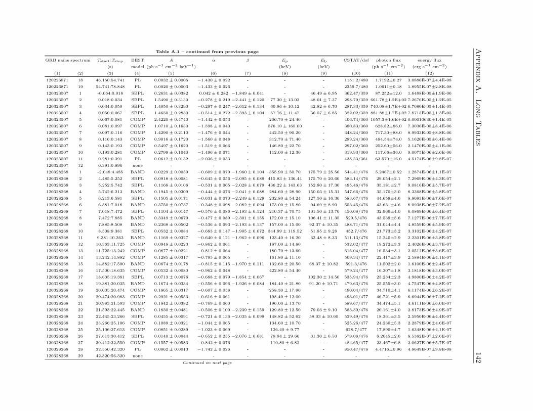
Appendix
A.
Long
Tables
142Table A.1 – continued from previous page
GRB name spectrum Tstart:Tstop BEST A α β Ep Eb CSTAT/dof photon flux energy flux
(s) model (ph s−1 cm−2 keV−1) (keV) (keV) (ph s−1 cm−2) (erg s−1 cm−2)
(1) (2) (3) (4) (5) (6) (7) (8) (9) (10) (11) (12)
120226871 18 46.150:54.741 PL 0.0032± 0.0005 −1.430± 0.022 - - - 1151.2/480 1.7192±0.27 3.0880E-07±4.4E-08
120226871 19 54.741:78.848 PL 0.0020± 0.0003 −1.433± 0.026 - - - 2359.7/480 1.0611±0.18 1.8955E-07±2.8E-08
120323507 1 -0.064:0.018 SBPL 0.2631± 0.0382 0.042± 0.282 −1.849± 0.041 - 46.49± 6.95 362.47/359 87.252±12.0 1.6488E-05±1.9E-06
120323507 2 0.018:0.034 SBPL 1.5490± 0.3130 −0.278± 0.219 −2.441± 0.120 77.30± 13.03 48.01± 7.37 298.79/359 661.78±1.2E+02 7.2676E-05±1.2E-05
120323507 3 0.034:0.050 SBPL 1.4050± 0.3290 −0.297± 0.247 −2.612± 0.134 60.86± 10.12 42.82± 6.70 287.33/359 740.08±1.7E+02 6.7080E-05±1.4E-05
120323507 4 0.050:0.067 SBPL 1.4650± 0.2830 −0.514± 0.272 −2.393± 0.104 57.76± 11.47 36.57± 6.85 322.02/359 881.88±1.7E+02 7.8715E-05±1.3E-05
120323507 5 0.067:0.081 COMP 2.4220± 0.4740 −1.442± 0.053 - 206.70± 24.40 - 406.74/360 1057.3±1.6E+02 0.00010630±1.4E-05
120323507 6 0.081:0.097 COMP 1.0710± 0.1630 −1.598± 0.040 - 576.10± 165.00 - 380.83/360 628.82±86.0 7.3036E-05±8.4E-06
120323507 7 0.097:0.116 COMP 1.4290± 0.2110 −1.476± 0.044 - 442.50± 90.20 - 348.24/360 717.30±88.0 8.9933E-05±8.8E-06
120323507 8 0.116:0.143 COMP 0.9016± 0.1720 −1.560± 0.048 - 312.70± 71.40 - 289.24/360 484.54±74.0 5.1620E-05±6.4E-06
120323507 9 0.143:0.193 COMP 0.5497± 0.1620 −1.519± 0.066 - 146.80± 22.70 - 297.02/360 252.60±56.0 2.1470E-05±4.1E-06
120323507 10 0.193:0.281 COMP 0.2799± 0.1040 −1.496± 0.071 - 112.00± 12.30 - 319.93/360 117.66±36.0 9.0075E-06±2.6E-06
120323507 11 0.281:0.391 PL 0.0612± 0.0132 −2.036± 0.033 - - - 438.33/361 63.570±16.0 4.5174E-06±9.8E-07
120323507 12 0.391:0.896 none - - - - - - - -
120328268 1 -2.048:4.485 BAND 0.0229± 0.0039 −0.609± 0.079 −1.960± 0.104 355.90± 50.70 175.79± 25.56 544.41/476 5.2467±0.52 1.2874E-06±1.1E-07
120328268 2 4.485:5.252 SBPL 0.0918± 0.0081 −0.645± 0.056 −2.095± 0.089 415.83± 136.44 175.70± 20.60 583.14/476 29.054±2.1 7.2969E-06±4.3E-07
120328268 3 5.252:5.742 SBPL 0.1168± 0.0106 −0.531± 0.065 −2.028± 0.079 436.22± 143.63 152.80± 17.30 495.46/476 35.181±2.7 9.0816E-06±5.7E-07
120328268 4 5.742:6.213 BAND 0.1945± 0.0309 −0.444± 0.076 −2.041± 0.088 284.60± 28.90 150.03± 15.31 547.66/476 35.170±3.0 8.3368E-06±5.8E-07
120328268 5 6.213:6.581 SBPL 0.1505± 0.0171 −0.631± 0.070 −2.249± 0.129 232.80± 54.24 127.50± 16.30 583.67/476 44.659±4.6 8.8083E-06±7.6E-07
120328268 6 6.581:7.018 BAND 0.3750± 0.0737 −0.348± 0.098 −2.082± 0.094 173.00± 15.80 94.69± 8.90 553.45/476 43.631±4.6 8.0938E-06±7.2E-07
120328268 7 7.018:7.472 SBPL 0.1104± 0.0147 −0.576± 0.086 −2.183± 0.124 210.37± 70.75 101.50± 13.70 450.08/476 32.966±4.0 6.0869E-06±6.4E-07
120328268 8 7.472:7.885 BAND 0.3349± 0.0679 −0.477± 0.089 −2.301± 0.155 172.00± 15.10 106.41± 11.35 529.5/476 43.539±5.6 7.1277E-06±7.7E-07
120328268 9 7.885:8.508 BAND 0.2368± 0.0502 −0.536± 0.093 −2.193± 0.137 157.00± 15.00 92.37± 10.35 488.71/476 31.044±4.4 4.8559E-06±5.9E-07
120328268 10 8.508:9.381 SBPL 0.0532± 0.0084 −0.683± 0.147 −1.905± 0.072 344.99± 119.52 51.85± 9.28 452.7/476 21.773±3.2 3.3102E-06±4.2E-07
120328268 11 9.381:10.363 BAND 0.1169± 0.0327 −0.640± 0.121 −1.962± 0.096 123.40± 16.20 63.48± 8.33 511.13/476 15.240±2.9 2.2301E-06±3.8E-07
120328268 12 10.363:11.725 COMP 0.0948± 0.0223 −0.862± 0.061 - 187.00± 14.80 - 532.02/477 19.272±3.3 2.4026E-06±3.7E-07
120328268 13 11.725:13.242 COMP 0.0877± 0.0221 −0.812± 0.064 - 180.70± 13.60 - 616.04/477 16.534±3.1 2.0512E-06±3.6E-07
120328268 14 13.242:14.882 COMP 0.1285± 0.0317 −0.795± 0.065 - 161.80± 11.10 - 509.34/477 22.417±3.9 2.5884E-06±4.1E-07
120328268 15 14.882:17.500 BAND 0.0674± 0.0178 −0.815± 0.115 −1.970± 0.111 132.60± 20.50 68.37± 10.82 591.3/476 11.502±2.0 1.6100E-06±2.4E-07
120328268 16 17.500:18.635 COMP 0.0532± 0.0080 −0.962± 0.048 - 422.80± 54.40 - 579.24/477 16.307±1.8 3.1818E-06±3.0E-07
120328268 17 18.635:19.381 SBPL 0.0713± 0.0076 −0.688± 0.079 −1.854± 0.067 - 102.30± 14.50 535.94/476 23.234±2.3 4.9800E-06±4.2E-07
120328268 18 19.381:20.035 BAND 0.1674± 0.0334 −0.556± 0.096 −1.926± 0.084 184.40± 21.80 91.20± 10.71 479.63/476 25.555±3.0 4.7547E-06±4.8E-07
120328268 19 20.035:20.474 COMP 0.1865± 0.0317 −0.607± 0.058 - 258.30± 17.90 - 490.04/477 34.710±4.1 6.1174E-06±6.2E-07
120328268 20 20.474:20.983 COMP 0.2921± 0.0553 −0.616± 0.061 - 198.40± 12.00 - 493.01/477 46.721±5.9 6.6944E-06±7.2E-07
120328268 21 20.983:21.593 COMP 0.1842± 0.0382 −0.769± 0.060 - 196.00± 13.70 - 589.67/477 34.474±5.1 4.6111E-06±6.0E-07
120328268 22 21.593:22.445 BAND 0.1830± 0.0481 −0.506± 0.109 −2.239± 0.159 129.80± 12.50 79.03± 9.10 583.39/476 20.161±4.0 2.8173E-06±4.9E-07
120328268 23 22.445:23.266 SBPL 0.0455± 0.0091 −0.721± 0.136 −2.035± 0.099 148.82± 52.62 58.03± 10.60 529.49/476 18.361±3.5 2.5950E-06±4.4E-07
120328268 24 23.266:25.106 COMP 0.1089± 0.0321 −1.044± 0.065 - 134.60± 10.70 - 525.26/477 24.230±5.3 2.2879E-06±4.6E-07
120328268 25 25.106:27.613 COMP 0.0851± 0.0289 −1.023± 0.069 - 126.40± 9.77 - 628.7/477 17.890±4.7 1.6348E-06±4.1E-07
120328268 26 27.613:30.412 SBPL 0.0140± 0.0044 −0.652± 0.255 −2.076± 0.081 79.94± 29.60 31.30± 6.50 579.08/476 8.2045±2.6 8.5382E-07±2.6E-07
120328268 27 30.412:32.550 COMP 0.1557± 0.0583 −0.842± 0.076 - 110.80± 6.82 - 484.65/477 23.467±6.8 2.0627E-06±5.7E-07
120328268 28 32.550:42.320 PL 0.0062± 0.0013 −1.742± 0.026 - - - 850.47/478 4.4716±0.96 4.8649E-07±9.8E-08
120328268 29 42.320:56.320 none - - - - - - - -
Continued on next page
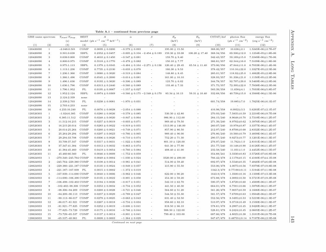
Appendix
A.
Long
Tables
143Table A.1 – continued from previous page
GRB name spectrum Tstart:Tstop BEST A α β Ep Eb CSTAT/dof photon flux energy flux
(s) model (ph s−1 cm−2 keV−1) (keV) (keV) (ph s−1 cm−2) (erg s−1 cm−2)
(1) (2) (3) (4) (5) (6) (7) (8) (9) (10) (11) (12)
120426090 1 -2.048:0.501 COMP 0.0699± 0.0200 −0.579± 0.093 - 195.00± 15.50 - 368.06/357 10.638±2.1 1.5245E-06±2.7E-07
120426090 2 0.501:0.638 SBPL 0.2352± 0.0457 −0.605± 0.104 −2.454± 0.189 159.36± 33.08 106.20± 17.40 368.34/356 69.506±12.0 1.1234E-05±1.8E-06
120426090 3 0.638:0.800 COMP 0.4610± 0.1450 −0.547± 0.081 - 159.70± 9.40 - 342.43/357 59.189±15.0 7.3349E-06±1.7E-06
120426090 4 0.800:0.975 COMP 0.5518± 0.1770 −0.478± 0.082 - 150.10± 7.77 - 366.81/357 62.344±16.0 7.5109E-06±1.8E-06
120426090 5 0.975:1.113 SBPL 0.1378± 0.0345 −0.484± 0.164 −2.271± 0.136 120.40± 29.45 65.54± 11.40 373.06/356 47.844±11.0 6.7033E-06±1.4E-06
120426090 6 1.113:1.236 COMP 0.7735± 0.2130 −0.633± 0.078 - 160.30± 9.53 - 378.42/357 110.16±22.0 1.3327E-05±2.5E-06
120426090 7 1.236:1.366 COMP 1.0080± 0.3020 −0.519± 0.084 - 148.80± 8.45 - 285.01/357 118.92±25.0 1.4062E-05±2.8E-06
120426090 8 1.366:1.496 COMP 0.6545± 0.2000 −0.614± 0.081 - 161.00± 10.10 - 328.93/357 91.338±21.0 1.1150E-05±2.3E-06
120426090 9 1.496:1.636 COMP 0.9192± 0.3620 −0.506± 0.089 - 123.70± 6.02 - 344.78/357 92.797±29.0 9.5469E-06±2.9E-06
120426090 10 1.636:1.796 COMP 0.6313± 0.2440 −0.560± 0.089 - 133.40± 7.33 - 371.75/357 72.395±22.0 7.7838E-06±2.3E-06
120426090 11 1.796:1.952 PL 0.0195± 0.0067 −1.557± 0.027 - - - 583.39/358 11.658±4.1 1.7033E-06±5.8E-07
120426090 12 1.952:2.124 SBPL 0.0974± 0.0369 −0.566± 0.175 −2.548± 0.170 83.34± 16.13 59.31± 10.40 332.68/356 40.739±15.0 4.3568E-06±1.5E-06
120426090 13 2.124:2.339 none - - - - - - - -
120426090 14 2.339:2.703 PL 0.0238± 0.0081 −1.870± 0.031 - - - 601.74/358 19.885±7.0 1.7825E-06±6.1E-07
120426090 15 2.703:4.233 none - - - - - - - -
120426090 16 4.233:10.240 PL 0.0076± 0.0028 −2.054± 0.088 - - - 416.98/358 8.0932±3.5 5.6293E-07±2.1E-07
120526303 1 -1.024:6.385 COMP 0.0280± 0.0026 −0.578± 0.085 - 530.30± 42.80 - 270.93/240 7.5835±0.59 2.2218E-06±9.7E-08
120526303 2 6.385:11.512 COMP 0.0248± 0.0020 −0.847± 0.064 - 986.90± 112.00 - 284.15/240 8.9648±0.70 2.7318E-06±1.2E-07
120526303 3 11.512:16.215 COMP 0.0257± 0.0019 −0.603± 0.071 - 969.40± 79.50 - 271.39/240 8.9792±0.62 3.3976E-06±1.2E-07
120526303 4 16.215:20.014 COMP 0.0283± 0.0022 −0.919± 0.055 - 1313.00± 146.00 - 260.07/240 10.978±0.87 3.3377E-06±1.4E-07
120526303 5 20.014:25.264 COMP 0.0260± 0.0021 −0.749± 0.071 - 857.90± 86.50 - 212.97/240 8.8708±0.68 2.8332E-06±1.2E-07
120526303 6 25.264:29.294 COMP 0.0297± 0.0023 −0.766± 0.065 - 989.40± 96.00 - 276.86/240 10.560±0.79 3.4839E-06±1.4E-07
120526303 7 29.294:33.708 COMP 0.0306± 0.0026 −0.710± 0.074 - 752.20± 71.30 - 290.57/240 9.9273±0.77 3.1201E-06±1.3E-07
120526303 8 33.708:37.347 COMP 0.0317± 0.0031 −1.022± 0.063 - 801.10± 120.00 - 276.97/240 11.762±1.0 2.8101E-06±1.5E-07
120526303 9 37.347:41.384 COMP 0.0312± 0.0032 −0.863± 0.074 - 641.30± 77.90 - 251.77/240 10.148±0.90 2.6126E-06±1.4E-07
120526303 10 41.384:45.460 COMP 0.0419± 0.0054 −0.760± 0.084 - 408.40± 41.00 - 232.58/240 11.031±1.0 2.4452E-06±1.5E-07
120526303 11 45.460:66.560 PL 0.0046± 0.0009 −1.752± 0.059 - - - 354.88/241 3.3330±0.83 3.5726E-07±6.8E-08
120624933 1 -270.340:-245.764 COMP 0.0049± 0.0004 −1.030± 0.024 - 3320.00± 490.00 - 766.42/478 2.1178±0.15 6.4160E-07±4.1E-08
120624933 2 -245.764:-229.380 COMP 0.0108± 0.0014 −0.981± 0.041 - 514.00± 59.40 - 692.97/478 3.5540±0.35 7.4840E-07±6.6E-08
120624933 3 -229.380:-221.187 COMP 0.0135± 0.0024 −0.949± 0.057 - 415.90± 55.50 - 553.06/478 4.0675±0.56 7.9379E-07±9.8E-08
120624933 4 -221.187:-167.939 PL 0.0015± 0.0002 −1.372± 0.019 - - - 1342.3/479 0.77190±0.11 1.5194E-07±1.9E-08
120624933 5 -167.939:-114.690 COMP 0.0040± 0.0006 −0.962± 0.046 - 622.00± 90.20 - 1643.9/478 1.3500±0.16 3.1339E-07±3.3E-08
120624933 6 -114.690:-106.498 COMP 0.0135± 0.0022 −0.891± 0.058 - 454.30± 59.20 - 672.88/478 4.0092±0.50 8.5721E-07±9.3E-08
120624933 7 -106.498:-102.402 COMP 0.0194± 0.0026 −0.817± 0.051 - 542.10± 62.70 - 590.37/478 5.8720±0.60 1.4569E-06±1.3E-07
120624933 8 -102.402:-98.306 COMP 0.0253± 0.0034 −0.734± 0.052 - 441.50± 40.30 - 664.01/478 6.7591±0.66 1.5976E-06±1.3E-07
120624933 9 -98.306:-94.209 COMP 0.0269± 0.0028 −0.721± 0.046 - 564.60± 51.20 - 561.26/478 7.9057±0.59 2.1606E-06±1.3E-07
120624933 10 -94.209:-90.113 COMP 0.0257± 0.0029 −0.789± 0.047 - 544.50± 55.30 - 581.57/478 7.6709±0.63 1.9504E-06±1.3E-07
120624933 11 -90.113:-86.017 COMP 0.0278± 0.0025 −0.663± 0.043 - 631.40± 52.50 - 552.56/478 8.3495±0.53 2.5219E-06±1.3E-07
120624933 12 -86.017:-81.921 COMP 0.0267± 0.0018 −0.734± 0.034 - 958.60± 82.10 - 510.97/478 9.3718±0.49 3.1530E-06±1.3E-07
120624933 13 -81.921:-77.825 COMP 0.0252± 0.0019 −0.606± 0.041 - 818.50± 66.10 - 578.81/478 8.2997±0.45 2.9420E-06±1.3E-07
120624933 14 -77.825:-73.729 COMP 0.0175± 0.0016 −0.766± 0.044 - 988.50± 122.00 - 528.81/478 6.2424±0.45 2.0605E-06±1.2E-07
120624933 15 -73.729:-65.537 COMP 0.0137± 0.0014 −0.891± 0.041 - 799.40± 103.00 - 687.66/478 4.8025±0.38 1.3101E-06±8.7E-08
120624933 16 -65.537:-40.961 PL 0.0009± 0.0003 −1.364± 0.029 - - - 947.67/479 0.48755±0.14 9.7197E-08±2.5E-08
Continued on next page
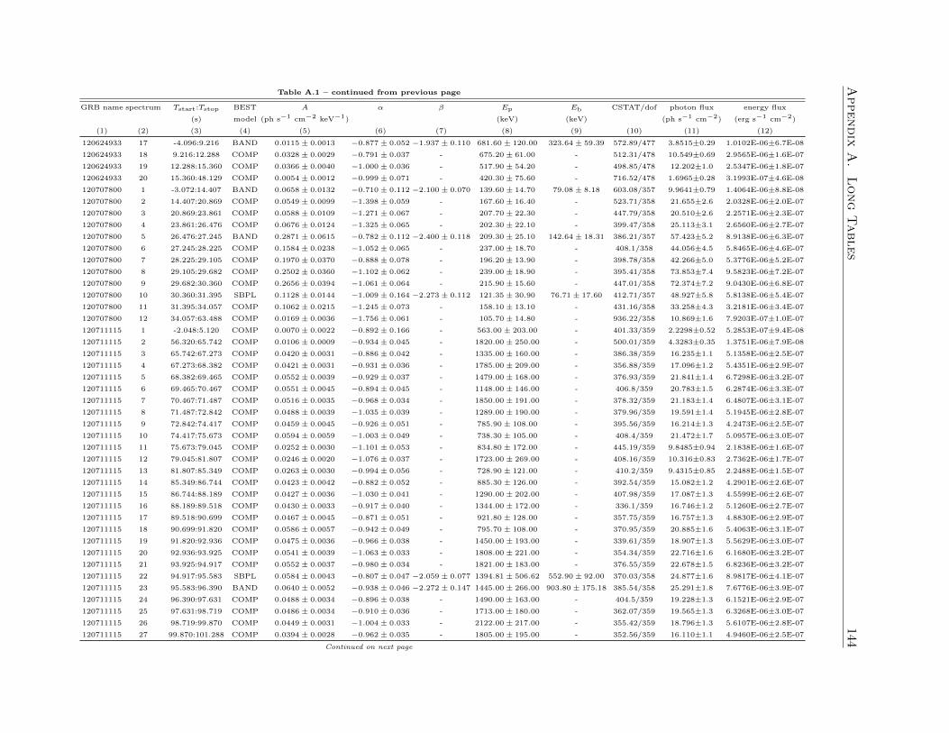
Appendix
A.
Long
Tables
144Table A.1 – continued from previous page
GRB name spectrum Tstart:Tstop BEST A α β Ep Eb CSTAT/dof photon flux energy flux
(s) model (ph s−1 cm−2 keV−1) (keV) (keV) (ph s−1 cm−2) (erg s−1 cm−2)
(1) (2) (3) (4) (5) (6) (7) (8) (9) (10) (11) (12)
120624933 17 -4.096:9.216 BAND 0.0115± 0.0013 −0.877± 0.052 −1.937± 0.110 681.60± 120.00 323.64± 59.39 572.89/477 3.8515±0.29 1.0102E-06±6.7E-08
120624933 18 9.216:12.288 COMP 0.0328± 0.0029 −0.791± 0.037 - 675.20± 61.00 - 512.31/478 10.549±0.69 2.9565E-06±1.6E-07
120624933 19 12.288:15.360 COMP 0.0366± 0.0040 −1.000± 0.036 - 517.90± 54.20 - 498.85/478 12.202±1.0 2.5347E-06±1.8E-07
120624933 20 15.360:48.129 COMP 0.0054± 0.0012 −0.999± 0.071 - 420.30± 75.60 - 716.52/478 1.6965±0.28 3.1993E-07±4.6E-08
120707800 1 -3.072:14.407 BAND 0.0658± 0.0132 −0.710± 0.112 −2.100± 0.070 139.60± 14.70 79.08± 8.18 603.08/357 9.9641±0.79 1.4064E-06±8.8E-08
120707800 2 14.407:20.869 COMP 0.0549± 0.0099 −1.398± 0.059 - 167.60± 16.40 - 523.71/358 21.655±2.6 2.0328E-06±2.0E-07
120707800 3 20.869:23.861 COMP 0.0588± 0.0109 −1.271± 0.067 - 207.70± 22.30 - 447.79/358 20.510±2.6 2.2571E-06±2.3E-07
120707800 4 23.861:26.476 COMP 0.0676± 0.0124 −1.325± 0.065 - 202.30± 22.10 - 399.47/358 25.113±3.1 2.6560E-06±2.7E-07
120707800 5 26.476:27.245 BAND 0.2871± 0.0615 −0.782± 0.112 −2.400± 0.118 209.30± 25.10 142.64± 18.31 386.21/357 57.423±5.2 8.9138E-06±6.3E-07
120707800 6 27.245:28.225 COMP 0.1584± 0.0238 −1.052± 0.065 - 237.00± 18.70 - 408.1/358 44.056±4.5 5.8465E-06±4.6E-07
120707800 7 28.225:29.105 COMP 0.1970± 0.0370 −0.888± 0.078 - 196.20± 13.90 - 398.78/358 42.266±5.0 5.3776E-06±5.2E-07
120707800 8 29.105:29.682 COMP 0.2502± 0.0360 −1.102± 0.062 - 239.00± 18.90 - 395.41/358 73.853±7.4 9.5823E-06±7.2E-07
120707800 9 29.682:30.360 COMP 0.2656± 0.0394 −1.061± 0.064 - 215.90± 15.60 - 447.01/358 72.374±7.2 9.0430E-06±6.8E-07
120707800 10 30.360:31.395 SBPL 0.1128± 0.0144 −1.009± 0.164 −2.273± 0.112 121.35± 30.90 76.71± 17.60 412.71/357 48.927±5.8 5.8138E-06±5.4E-07
120707800 11 31.395:34.057 COMP 0.1062± 0.0215 −1.245± 0.073 - 158.10± 13.10 - 431.16/358 33.258±4.3 3.2181E-06±3.4E-07
120707800 12 34.057:63.488 COMP 0.0169± 0.0036 −1.756± 0.061 - 105.70± 14.80 - 936.22/358 10.869±1.6 7.9203E-07±1.0E-07
120711115 1 -2.048:5.120 COMP 0.0070± 0.0022 −0.892± 0.166 - 563.00± 203.00 - 401.33/359 2.2298±0.52 5.2853E-07±9.4E-08
120711115 2 56.320:65.742 COMP 0.0106± 0.0009 −0.934± 0.045 - 1820.00± 250.00 - 500.01/359 4.3283±0.35 1.3751E-06±7.9E-08
120711115 3 65.742:67.273 COMP 0.0420± 0.0031 −0.886± 0.042 - 1335.00± 160.00 - 386.38/359 16.235±1.1 5.1358E-06±2.5E-07
120711115 4 67.273:68.382 COMP 0.0421± 0.0031 −0.931± 0.036 - 1785.00± 209.00 - 356.88/359 17.096±1.2 5.4351E-06±2.9E-07
120711115 5 68.382:69.465 COMP 0.0552± 0.0039 −0.929± 0.037 - 1479.00± 168.00 - 376.93/359 21.841±1.4 6.7298E-06±3.2E-07
120711115 6 69.465:70.467 COMP 0.0551± 0.0045 −0.894± 0.045 - 1148.00± 146.00 - 406.8/359 20.783±1.5 6.2874E-06±3.3E-07
120711115 7 70.467:71.487 COMP 0.0516± 0.0035 −0.968± 0.034 - 1850.00± 191.00 - 378.32/359 21.183±1.4 6.4807E-06±3.1E-07
120711115 8 71.487:72.842 COMP 0.0488± 0.0039 −1.035± 0.039 - 1289.00± 190.00 - 379.96/359 19.591±1.4 5.1945E-06±2.8E-07
120711115 9 72.842:74.417 COMP 0.0459± 0.0045 −0.926± 0.051 - 785.90± 108.00 - 395.56/359 16.214±1.3 4.2473E-06±2.5E-07
120711115 10 74.417:75.673 COMP 0.0594± 0.0059 −1.003± 0.049 - 738.30± 105.00 - 408.4/359 21.472±1.7 5.0957E-06±3.0E-07
120711115 11 75.673:79.045 COMP 0.0252± 0.0030 −1.101± 0.053 - 834.80± 172.00 - 445.19/359 9.8485±0.94 2.1838E-06±1.6E-07
120711115 12 79.045:81.807 COMP 0.0246± 0.0020 −1.076± 0.037 - 1723.00± 269.00 - 408.16/359 10.316±0.83 2.7362E-06±1.7E-07
120711115 13 81.807:85.349 COMP 0.0263± 0.0030 −0.994± 0.056 - 728.90± 121.00 - 410.2/359 9.4315±0.85 2.2488E-06±1.5E-07
120711115 14 85.349:86.744 COMP 0.0423± 0.0042 −0.882± 0.052 - 885.30± 126.00 - 392.54/359 15.082±1.2 4.2901E-06±2.6E-07
120711115 15 86.744:88.189 COMP 0.0427± 0.0036 −1.030± 0.041 - 1290.00± 202.00 - 407.98/359 17.087±1.3 4.5599E-06±2.6E-07
120711115 16 88.189:89.518 COMP 0.0430± 0.0033 −0.917± 0.040 - 1344.00± 172.00 - 336.1/359 16.746±1.2 5.1260E-06±2.7E-07
120711115 17 89.518:90.699 COMP 0.0467± 0.0045 −0.871± 0.051 - 921.80± 128.00 - 357.75/359 16.757±1.3 4.8830E-06±2.9E-07
120711115 18 90.699:91.820 COMP 0.0586± 0.0057 −0.942± 0.049 - 795.70± 108.00 - 370.95/359 20.885±1.6 5.4063E-06±3.1E-07
120711115 19 91.820:92.936 COMP 0.0475± 0.0036 −0.966± 0.038 - 1450.00± 193.00 - 339.61/359 18.907±1.3 5.5629E-06±3.0E-07
120711115 20 92.936:93.925 COMP 0.0541± 0.0039 −1.063± 0.033 - 1808.00± 221.00 - 354.34/359 22.716±1.6 6.1680E-06±3.2E-07
120711115 21 93.925:94.917 COMP 0.0552± 0.0037 −0.980± 0.034 - 1821.00± 183.00 - 376.55/359 22.678±1.5 6.8236E-06±3.2E-07
120711115 22 94.917:95.583 SBPL 0.0584± 0.0043 −0.807± 0.047 −2.059± 0.077 1394.81± 506.62 552.90± 92.00 370.03/358 24.877±1.6 8.9817E-06±4.1E-07
120711115 23 95.583:96.390 BAND 0.0640± 0.0052 −0.938± 0.046 −2.272± 0.147 1445.00± 266.00 903.80± 175.18 385.54/358 25.291±1.8 7.6776E-06±3.9E-07
120711115 24 96.390:97.631 COMP 0.0488± 0.0034 −0.896± 0.038 - 1490.00± 163.00 - 404.5/359 19.228±1.3 6.1521E-06±2.9E-07
120711115 25 97.631:98.719 COMP 0.0486± 0.0034 −0.910± 0.036 - 1713.00± 180.00 - 362.07/359 19.565±1.3 6.3268E-06±3.0E-07
120711115 26 98.719:99.870 COMP 0.0449± 0.0031 −1.004± 0.033 - 2122.00± 217.00 - 355.42/359 18.796±1.3 5.6107E-06±2.8E-07
120711115 27 99.870:101.288 COMP 0.0394± 0.0028 −0.962± 0.035 - 1805.00± 195.00 - 352.56/359 16.110±1.1 4.9460E-06±2.5E-07
Continued on next page
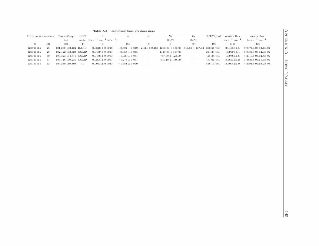
Appendix
A.
Long
Tables
145Table A.1 – continued from previous page
GRB name spectrum Tstart:Tstop BEST A α β Ep Eb CSTAT/dof photon flux energy flux
(s) model (ph s−1 cm−2 keV−1) (keV) (keV) (ph s−1 cm−2) (erg s−1 cm−2)
(1) (2) (3) (4) (5) (6) (7) (8) (9) (10) (11) (12)
120711115 28 101.288:102.122 BAND 0.0618± 0.0048 −0.807± 0.049 −2.414± 0.163 1263.00± 183.00 849.68± 137.94 366.67/358 23.403±1.5 7.9374E-06±3.7E-07
120711115 29 102.122:103.323 COMP 0.0469± 0.0041 −0.965± 0.045 - 1117.00± 167.00 - 354.33/359 17.990±1.4 5.0084E-06±2.9E-07
120711115 30 103.323:104.716 COMP 0.0488± 0.0053 −1.023± 0.051 - 767.30± 123.00 - 415.34/359 17.988±1.6 4.2310E-06±2.8E-07
120711115 31 104.716:109.230 COMP 0.0205± 0.0037 −1.275± 0.061 - 535.10± 139.00 - 471.01/359 8.5653±1.2 1.3835E-06±1.5E-07
120711115 32 109.230:119.808 PL 0.0053± 0.0013 −1.681± 0.060 - - - 518.13/360 3.6005±1.0 4.2991E-07±9.2E-08
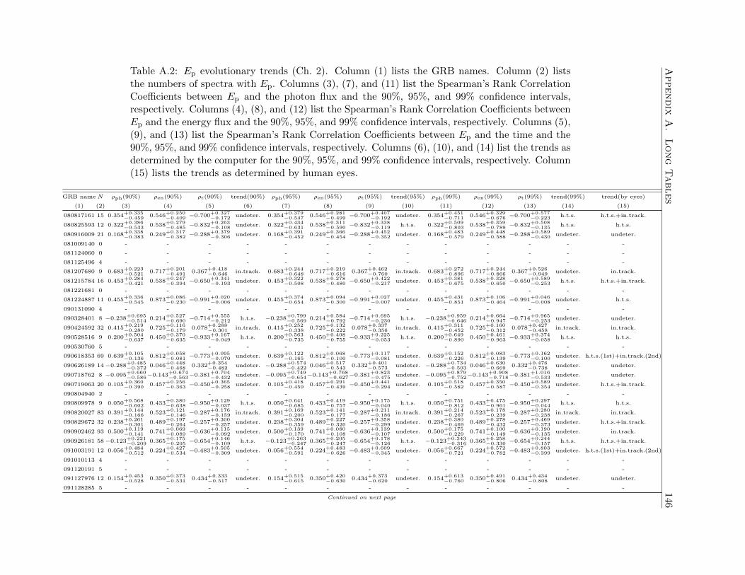
Appendix
A.
Long
Tables
146Table A.2: Ep evolutionary trends (Ch. 2). Column (1) lists the GRB names. Column (2) liststhe numbers of spectra with Ep. Columns (3), (7), and (11) list the Spearman’s Rank CorrelationCoefficients between Ep and the photon flux and the 90%, 95%, and 99% confidence intervals,respectively. Columns (4), (8), and (12) list the Spearman’s Rank Correlation Coefficients betweenEp and the energy flux and the 90%, 95%, and 99% confidence intervals, respectively. Columns (5),(9), and (13) list the Spearman’s Rank Correlation Coefficients between Ep and the time and the90%, 95%, and 99% confidence intervals, respectively. Columns (6), (10), and (14) list the trends asdetermined by the computer for the 90%, 95%, and 99% confidence intervals, respectively. Column(15) lists the trends as determined by human eyes.
GRB nameN ρph(90%) ρen(90%) ρt(90%) trend(90%) ρph(95%) ρen(95%) ρt(95%) trend(95%) ρph(99%) ρen(99%) ρt(99%) trend(99%) trend(by eyes)
(1) (2) (3) (4) (5) (6) (7) (8) (9) (10) (11) (12) (13) (14) (15)
080817161 15 0.354+0.335−0.459 0.546+0.250
−0.409 −0.700+0.327−0.172 undeter. 0.354+0.379
−0.547 0.546+0.281−0.499 −0.700+0.407
−0.192 undeter. 0.354+0.451−0.711 0.546+0.329
−0.676 −0.700+0.577−0.223 h.t.s. h.t.s.+in.track.
080825593 12 0.322+0.386−0.533 0.538+0.279
−0.485 −0.832+0.263−0.108 undeter. 0.322+0.434
−0.631 0.538+0.311−0.590 −0.832+0.338
−0.119 h.t.s. 0.322+0.509−0.803 0.538+0.359
−0.789 −0.832+0.508−0.135 h.t.s. h.t.s.
080916009 21 0.168+0.338−0.383 0.249+0.317
−0.382 −0.288+0.379−0.306 undeter. 0.168+0.391
−0.452 0.249+0.366−0.454 −0.288+0.452
−0.352 undeter. 0.168+0.483−0.579 0.249+0.448
−0.588 −0.288+0.589−0.430 undeter. undeter.
081009140 0 - - - - - - - - - - - - -
081124060 0 - - - - - - - - - - - - -
081125496 4 - - - - - - - - - - - - -
081207680 9 0.683+0.223−0.521 0.717+0.201
−0.491 0.367+0.418−0.646 in.track. 0.683+0.244
−0.648 0.717+0.219−0.616 0.367+0.462
−0.760 in.track. 0.683+0.272−0.896 0.717+0.244
−0.866 0.367+0.526−0.949 undeter. in.track.
081215784 16 0.453+0.284−0.421 0.538+0.247
−0.394 −0.650+0.341−0.193 undeter. 0.453+0.322
−0.508 0.538+0.278−0.480 −0.650+0.422
−0.217 undeter. 0.453+0.381−0.675 0.538+0.328
−0.650 −0.650+0.589−0.253 h.t.s. h.t.s.+in.track.
081221681 0 - - - - - - - - - - - - -
081224887 11 0.455+0.336−0.545 0.873+0.086
−0.230 −0.991+0.020−0.006 undeter. 0.455+0.374
−0.654 0.873+0.094−0.300 −0.991+0.027
−0.007 undeter. 0.455+0.431−0.851 0.873+0.106
−0.464 −0.991+0.046−0.008 undeter. h.t.s.
090131090 4 - - - - - - - - - - - - -
090328401 8 −0.238+0.695−0.514 0.214+0.527
−0.690 −0.714+0.555−0.212 h.t.s. −0.238+0.799
−0.569 0.214+0.584−0.792 −0.714+0.695
−0.230 h.t.s. −0.238+0.959−0.646 0.214+0.664
−0.947 −0.714+0.965−0.253 undeter. undeter.
090424592 32 0.415+0.219−0.280 0.725+0.116
−0.179 0.078+0.288−0.301 in.track. 0.415+0.252
−0.338 0.725+0.132−0.222 0.078+0.337
−0.356 in.track. 0.415+0.311−0.452 0.725+0.160
−0.312 0.078+0.427−0.458 in.track. in.track.
090528516 9 0.200+0.504−0.637 0.450+0.370
−0.635 −0.933+0.167−0.049 h.t.s. 0.200+0.563
−0.735 0.450+0.408−0.755 −0.933+0.225
−0.053 h.t.s. 0.200+0.649−0.890 0.450+0.461
−0.963 −0.933+0.374−0.058 h.t.s. h.t.s.
090530760 5 - - - - - - - - - - - - -
090618353 69 0.639+0.105−0.136 0.812+0.058
−0.081 −0.773+0.095−0.070 undeter. 0.639+0.122
−0.165 0.812+0.068−0.100 −0.773+0.117
−0.081 undeter. 0.639+0.152−0.226 0.812+0.083
−0.139 −0.773+0.162−0.100 undeter. h.t.s.(1st)+in.track.(2nd)
090626189 14−0.288+0.485−0.372 0.046+0.448
−0.468 0.332+0.354−0.482 undeter. −0.288+0.574
−0.422 0.046+0.517−0.543 0.332+0.401
−0.573 undeter. −0.288+0.734−0.503 0.046+0.630
−0.669 0.332+0.476−0.738 undeter. undeter.
090718762 8 −0.095+0.660−0.586−0.143+0.674
−0.563−0.381+0.704−0.432 undeter. −0.095+0.749
−0.654−0.143+0.768−0.627−0.381+0.823
−0.475 undeter. −0.095+0.879−0.752−0.143+0.908
−0.718−0.381+1.016−0.533 undeter. undeter.
090719063 20 0.105+0.360−0.390 0.457+0.256
−0.363 −0.450+0.365−0.258 undeter. 0.105+0.418
−0.459 0.457+0.291−0.439 −0.450+0.441
−0.294 undeter. 0.105+0.518−0.582 0.457+0.350
−0.587 −0.450+0.589−0.354 undeter. h.t.s.+in.track.
090804940 2 - - - - - - - - - - - - -
090809978 9 0.050+0.568−0.602 0.433+0.380
−0.638 −0.950+0.129−0.037 h.t.s. 0.050+0.641
−0.685 0.433+0.419−0.757 −0.950+0.175
−0.040 h.t.s. 0.050+0.751−0.812 0.433+0.475
−0.961 −0.950+0.297−0.044 h.t.s. h.t.s.
090820027 83 0.391+0.144−0.166 0.523+0.121
−0.146 −0.287+0.176−0.159 in.track. 0.391+0.169
−0.200 0.523+0.141−0.177 −0.287+0.211
−0.186 in.track. 0.391+0.214−0.267 0.523+0.178
−0.239 −0.287+0.280−0.238 in.track. in.track.
090829672 32 0.238+0.261−0.301 0.489+0.197
−0.264 −0.257+0.300−0.257 undeter. 0.238+0.304
−0.359 0.489+0.227−0.320 −0.257+0.358
−0.299 undeter. 0.238+0.380−0.469 0.489+0.278
−0.432 −0.257+0.469−0.373 undeter. h.t.s.+in.track.
090902462 93 0.500+0.119−0.141 0.741+0.069
−0.089 −0.636+0.115−0.092 undeter. 0.500+0.139
−0.170 0.741+0.080−0.108 −0.636+0.139
−0.107 undeter. 0.500+0.175−0.229 0.741+0.100
−0.149 −0.636+0.190−0.135 undeter. in.track.
090926181 58−0.123+0.221−0.209 0.365+0.175
−0.205 −0.654+0.146−0.109 h.t.s. −0.123+0.263
−0.247 0.365+0.205−0.247 −0.654+0.178
−0.126 h.t.s. −0.123+0.343−0.316 0.365+0.258
−0.330 −0.654+0.244−0.157 h.t.s. h.t.s.+in.track.
091003191 12 0.056+0.484−0.512 0.224+0.427
−0.534 −0.483+0.505−0.309 undeter. 0.056+0.554
−0.591 0.224+0.483−0.626 −0.483+0.609
−0.345 undeter. 0.056+0.667−0.721 0.224+0.572
−0.782 −0.483+0.803−0.399 undeter. h.t.s.(1st)+in.track.(2nd)
091010113 4 - - - - - - - - - - - - -
091120191 5 - - - - - - - - - - - - -
091127976 12 0.154+0.453−0.528 0.350+0.373
−0.531 0.434+0.333−0.517 undeter. 0.154+0.515
−0.615 0.350+0.420−0.630 0.434+0.373
−0.620 undeter. 0.154+0.613−0.760 0.350+0.491
−0.806 0.434+0.434−0.808 undeter. undeter.
091128285 5 - - - - - - - - - - - - -
Continued on next page

Appendix
A.
Long
Tables
147Table A.2 – continued from previous page
GRB nameN ρph(90%) ρen(90%) ρt(90%) trend(90%) ρph(95%) ρen(95%) ρt(95%) trend(95%) ρph(99%) ρen(99%) ρt(99%) trend(99%) trend(by eyes)
(1) (2) (3) (4) (5) (6) (7) (8) (9) (10) (11) (12) (13) (14) (15)
100122616 2 - - - - - - - - - - - - -
100322045 19−0.263+0.404−0.329 0.672+0.169
−0.289 0.668+0.171−0.291 in.track. −0.263+0.480
−0.378 0.672+0.191−0.359 0.668+0.193
−0.361 in.track. −0.263+0.621−0.460 0.672+0.225
−0.503 0.668+0.228−0.506 in.track. in.track.(2nd)
100324172 9 0.200+0.504−0.637 0.367+0.418
−0.646 −0.883+0.267−0.085 h.t.s. 0.200+0.563
−0.735 0.367+0.462−0.760 −0.883+0.353
−0.092 h.t.s. 0.200+0.649−0.890 0.367+0.526
−0.949 −0.883+0.556−0.102 h.t.s. h.t.s.
100414097 15−0.200+0.466−0.390−0.025+0.447
−0.437−0.093+0.457−0.421 undeter. −0.200+0.548
−0.446−0.025+0.519−0.505−0.093+0.533
−0.485 undeter. −0.200+0.693−0.538−0.025+0.641
−0.621−0.093+0.665−0.591 undeter. undeter.
100511035 3 - - - - - - - - - - - - -
100612726 4 - - - - - - - - - - - - -
100707032 25 0.406+0.248−0.326 0.770+0.109
−0.185 −0.936+0.061−0.032 undeter. 0.406+0.284
−0.393 0.770+0.123−0.231 −0.936+0.078
−0.036 undeter. 0.406+0.347−0.524 0.770+0.147
−0.331 −0.936+0.116−0.042 undeter. h.t.s.
100719989 14 0.332+0.354−0.482 0.499+0.280
−0.447 −0.776+0.284−0.135 h.t.s. 0.332+0.401
−0.573 0.499+0.315−0.542 −0.776+0.359
−0.150 h.t.s. 0.332+0.476−0.738 0.499+0.369
−0.724 −0.776+0.523−0.172 h.t.s. in.track.
100722096 1 - - - - - - - - - - - - -
100724029 47 0.397+0.187−0.227 0.455+0.173
−0.217 −0.245+0.243−0.216 undeter. 0.397+0.217
−0.273 0.455+0.201−0.262 −0.245+0.290
−0.252 undeter. 0.397+0.272−0.365 0.455+0.251
−0.353 −0.245+0.382−0.319 undeter. in.track.
100728095 21 0.474+0.244−0.347 0.741+0.131
−0.229 −0.537+0.328−0.219 undeter. 0.474+0.278
−0.421 0.741+0.147−0.286 −0.537+0.400
−0.249 undeter. 0.474+0.334−0.565 0.741+0.174
−0.408 −0.537+0.544−0.299 in.track. in.track.
100826957 21 0.165+0.339−0.383 0.318+0.297
−0.376 0.031+0.365−0.373 undeter. 0.165+0.392
−0.452 0.318+0.341−0.450 0.031+0.426
−0.437 undeter. 0.165+0.484−0.579 0.318+0.415
−0.589 0.031+0.532−0.551 undeter. in.track.
100829876 5 - - - - - - - - - - - - -
100910818 5 - - - - - - - - - - - - -
100918863 26 0.762+0.111−0.185 0.843+0.075
−0.133 0.162+0.305−0.340 in.track. 0.762+0.125
−0.230 0.843+0.085−0.167 0.162+0.355
−0.402 in.track. 0.762+0.150−0.329 0.843+0.101
−0.242 0.162+0.443−0.519 in.track. in.track.
101014175 43 0.236+0.227−0.256 0.506+0.168
−0.217 0.090+0.247−0.258 in.track. 0.236+0.265
−0.305 0.506+0.194−0.264 0.090+0.290
−0.306 in.track. 0.236+0.334−0.401 0.506+0.240
−0.357 0.090+0.370−0.397 in.track. h.t.s.+in.track.
101023951 10 0.709+0.197−0.451 0.818+0.126
−0.333 −0.285+0.602−0.439 in.track. 0.709+0.216
−0.566 0.818+0.137−0.429 −0.285+0.705
−0.491 in.track. 0.709+0.243−0.797 0.818+0.154
−0.642 −0.285+0.877−0.568 in.track. in.track.
101123952 39 0.369+0.210−0.256 0.496+0.178
−0.233 −0.521+0.226−0.171 h.t.s. 0.369+0.244
−0.308 0.496+0.206−0.282 −0.521+0.275
−0.197 h.t.s. 0.369+0.304−0.411 0.496+0.254
−0.382 −0.521+0.373−0.243 h.t.s. h.t.s.+in.track.
101126198 11−0.536+0.519−0.291−0.273+0.566
−0.424−0.264+0.566−0.428 undeter. −0.536+0.630
−0.323−0.273+0.664−0.477−0.264+0.663
−0.482 undeter. −0.536+0.838−0.370−0.273+0.831
−0.558−0.264+0.829−0.564 undeter. undeter.
101231067 4 - - - - - - - - - - - - -
110213220 0 - - - - - - - - - - - - -
110301214 27−0.042+0.328−0.319 0.031+0.320
−0.327 −0.315+0.325−0.265 undeter. −0.042+0.385
−0.373 0.031+0.375−0.384 −0.315+0.389
−0.306 undeter. −0.042+0.491−0.472 0.031+0.475
−0.489 −0.315+0.512−0.377 undeter. h.t.s.+in.track.
110407998 5 - - - - - - - - - - - - -
110428388 5 - - - - - - - - - - - - -
110622158 14−0.086+0.474−0.438−0.042+0.467
−0.450−0.459+0.459−0.299 undeter. −0.086+0.552
−0.504−0.042+0.542−0.518−0.459+0.554
−0.337 undeter. −0.086+0.684−0.612−0.042+0.668
−0.632−0.459+0.732−0.395 undeter. undeter.
110625881 38−0.007+0.272−0.271 0.311+0.226
−0.267 −0.439+0.248−0.196 undeter. −0.007+0.320
−0.319 0.311+0.263−0.321 −0.439+0.300
−0.226 undeter. −0.007+0.411−0.408 0.311+0.328
−0.424 −0.439+0.403−0.280 undeter. in.track.
110717319 13 0.363+0.354−0.502 0.615+0.229
−0.421 −0.011+0.480−0.475 in.track. 0.363+0.399
−0.598 0.615+0.256−0.518 −0.011+0.554
−0.548 in.track. 0.363+0.469−0.772 0.615+0.295
−0.712 −0.011+0.677−0.667 undeter. in.track.
110721200 12−0.538+0.485−0.279 0.049+0.486
−0.511 −0.490+0.502−0.305 undeter. −0.538+0.590
−0.311 0.049+0.557−0.589 −0.490+0.607
−0.341 undeter. −0.538+0.789−0.359 0.049+0.671
−0.718 −0.490+0.802−0.394 undeter. h.t.s.
110729142 7 0.571+0.329−0.743 0.607+0.303
−0.725 −0.107+0.721−0.623 undeter. 0.571+0.355
−0.890 0.607+0.326−0.876 −0.107+0.810
−0.689 undeter. 0.571+0.388−1.135 0.607+0.356
−1.132 −0.107+0.935−0.777 undeter. undeter.
110731465 7 −0.036+0.692−0.660 0.643+0.277
−0.702 0.929+0.057−0.251 undeter. −0.036+0.773
−0.732 0.643+0.298−0.856 0.929+0.061
−0.345 undeter. −0.036+0.884−0.832 0.643+0.325
−1.124 0.929+0.066−0.583 undeter. undeter.
110817191 4 - - - - - - - - - - - - -
110825102 20 0.087+0.364−0.389 0.720+0.143
−0.251 0.421+0.269−0.371 in.track. 0.087+0.423
−0.457 0.720+0.161−0.313 0.421+0.307
−0.447 in.track. 0.087+0.525−0.578 0.720+0.191
−0.444 0.421+0.370−0.595 in.track. in.track.
110903009 2 - - - - - - - - - - - - -
110920546 17 0.583+0.220−0.359 0.848+0.086
−0.179 −0.968+0.043−0.019 undeter. 0.583+0.248
−0.441 0.848+0.096−0.228 −0.968+0.056
−0.021 undeter. 0.583+0.292−0.604 0.848+0.111
−0.339 −0.968+0.089−0.024 undeter. h.t.s.
110921912 11−0.187+0.560−0.460−0.027+0.531
−0.516−0.437+0.550−0.345 undeter. −0.187+0.652
−0.521−0.027+0.609−0.590−0.437+0.658
−0.384 undeter. −0.187+0.805−0.613−0.027+0.735
−0.707−0.437+0.852−0.443 undeter. undeter.
111003465 6 0.086+0.690−0.784 0.714+0.237
−0.768 −0.829+0.599−0.144 h.t.s. 0.086+0.753
−0.866 0.714+0.252−0.946 −0.829+0.777
−0.152 h.t.s. 0.086+0.832−0.971 0.714+0.269
−1.245 −0.829+1.123−0.162 undeter. h.t.s.+in.track.
111127810 0 - - - - - - - - - - - - -
111216389 9 −0.167+0.631−0.519 0.483+0.350
−0.627 −0.600+0.578−0.277 h.t.s. −0.167+0.726
−0.581 0.483+0.385−0.750 −0.600+0.707
−0.304 undeter. −0.167+0.875−0.673 0.483+0.435
−0.964 −0.600+0.944−0.341 undeter. in.track.
111220486 9 0.483+0.350−0.627 0.650+0.245
−0.547 −0.317+0.647−0.445 in.track. 0.483+0.385
−0.750 0.650+0.268−0.675 −0.317+0.757
−0.494 undeter. 0.483+0.435−0.964 0.650+0.299
−0.919 −0.317+0.936−0.564 undeter. in.track.
111228657 1 - - - - - - - - - - - - -
120119170 15 0.475+0.283−0.433 0.743+0.149
−0.295 −0.450+0.440−0.294 in.track. 0.475+0.319
−0.524 0.743+0.166−0.371 −0.450+0.531
−0.332 in.track. 0.475+0.376−0.698 0.743+0.193
−0.533 −0.450+0.703−0.392 in.track. in.track.
120129580 29 0.390+0.236−0.301 0.600+0.168
−0.246 −0.083+0.318−0.302 in.track. 0.390+0.272
−0.363 0.600+0.192−0.301 −0.083+0.375
−0.353 in.track. 0.390+0.335−0.483 0.600+0.233
−0.414 −0.083+0.481−0.446 in.track. in.track.
120204054 44 0.216+0.227−0.253 0.547+0.155
−0.204 −0.136+0.255−0.239 in.track. 0.216+0.266
−0.302 0.547+0.179−0.249 −0.136+0.304
−0.280 in.track. 0.216+0.336−0.397 0.547+0.222
−0.338 −0.136+0.395−0.356 in.track. in.track.
Continued on next page
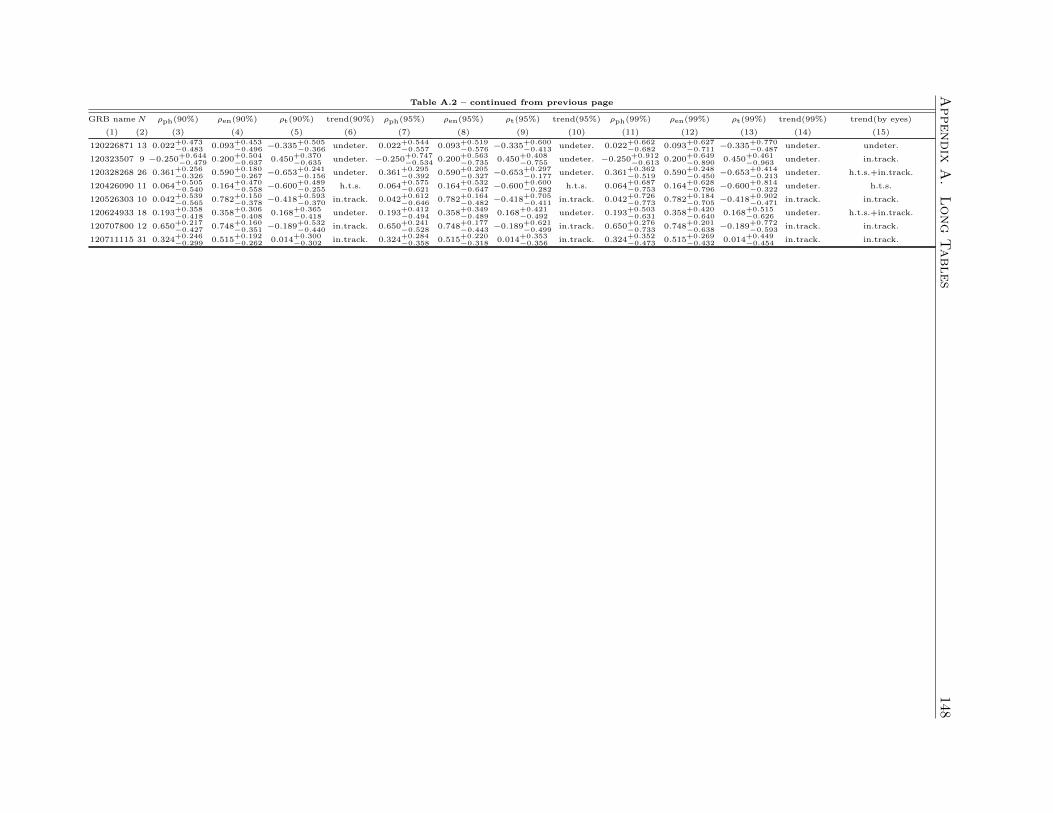
Appendix
A.
Long
Tables
148Table A.2 – continued from previous page
GRB nameN ρph(90%) ρen(90%) ρt(90%) trend(90%) ρph(95%) ρen(95%) ρt(95%) trend(95%) ρph(99%) ρen(99%) ρt(99%) trend(99%) trend(by eyes)
(1) (2) (3) (4) (5) (6) (7) (8) (9) (10) (11) (12) (13) (14) (15)
120226871 13 0.022+0.473−0.483 0.093+0.453
−0.496 −0.335+0.505−0.366 undeter. 0.022+0.544
−0.557 0.093+0.519−0.576 −0.335+0.600
−0.413 undeter. 0.022+0.662−0.682 0.093+0.627
−0.711 −0.335+0.770−0.487 undeter. undeter.
120323507 9 −0.250+0.644−0.479 0.200+0.504
−0.637 0.450+0.370−0.635 undeter. −0.250+0.747
−0.534 0.200+0.563−0.735 0.450+0.408
−0.755 undeter. −0.250+0.912−0.613 0.200+0.649
−0.890 0.450+0.461−0.963 undeter. in.track.
120328268 26 0.361+0.256−0.326 0.590+0.180
−0.267 −0.653+0.241−0.156 undeter. 0.361+0.295
−0.392 0.590+0.205−0.327 −0.653+0.297
−0.177 undeter. 0.361+0.362−0.519 0.590+0.248
−0.450 −0.653+0.414−0.213 undeter. h.t.s.+in.track.
120426090 11 0.064+0.505−0.540 0.164+0.470
−0.558 −0.600+0.489−0.255 h.t.s. 0.064+0.575
−0.621 0.164+0.532−0.647 −0.600+0.600
−0.282 h.t.s. 0.064+0.687−0.753 0.164+0.628
−0.796 −0.600+0.814−0.322 undeter. h.t.s.
120526303 10 0.042+0.539−0.565 0.782+0.150
−0.378 −0.418+0.593−0.370 in.track. 0.042+0.612
−0.646 0.782+0.164−0.482 −0.418+0.705
−0.411 in.track. 0.042+0.726−0.773 0.782+0.184
−0.705 −0.418+0.902−0.471 in.track. in.track.
120624933 18 0.193+0.358−0.418 0.358+0.306
−0.408 0.168+0.365−0.418 undeter. 0.193+0.412
−0.494 0.358+0.349−0.489 0.168+0.421
−0.492 undeter. 0.193+0.503−0.631 0.358+0.420
−0.640 0.168+0.515−0.626 undeter. h.t.s.+in.track.
120707800 12 0.650+0.217−0.427 0.748+0.160
−0.351 −0.189+0.532−0.440 in.track. 0.650+0.241
−0.528 0.748+0.177−0.443 −0.189+0.621
−0.499 in.track. 0.650+0.276−0.733 0.748+0.201
−0.638 −0.189+0.772−0.593 in.track. in.track.
120711115 31 0.324+0.246−0.299 0.515+0.192
−0.262 0.014+0.300−0.302 in.track. 0.324+0.284
−0.358 0.515+0.220−0.318 0.014+0.353
−0.356 in.track. 0.324+0.352−0.473 0.515+0.269
−0.432 0.014+0.449−0.454 in.track. in.track.
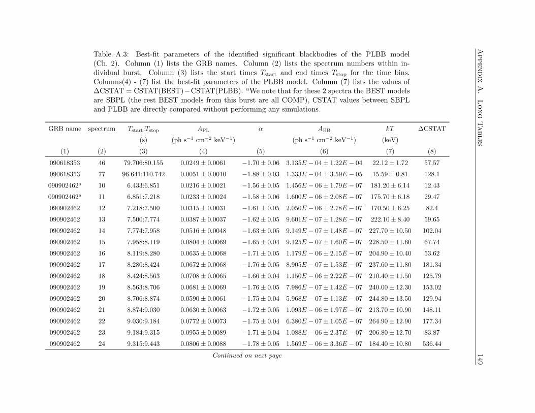
Appendix
A.
Long
Tables
149Table A.3: Best-fit parameters of the identified significant blackbodies of the PLBB model(Ch. 2). Column (1) lists the GRB names. Column (2) lists the spectrum numbers within in-dividual burst. Column (3) lists the start times Tstart and end times Tstop for the time bins.Columns(4) - (7) list the best-fit parameters of the PLBB model. Column (7) lists the values of∆CSTAT = CSTAT(BEST)−CSTAT(PLBB). aWe note that for these 2 spectra the BEST modelsare SBPL (the rest BEST models from this burst are all COMP), CSTAT values between SBPLand PLBB are directly compared without performing any simulations.
GRB name spectrum Tstart:Tstop APL α ABB kT ∆CSTAT
(s) (ph s−1 cm−2 keV−1) (ph s−1 cm−2 keV−1) (keV)
(1) (2) (3) (4) (5) (6) (7) (8)
090618353 46 79.706:80.155 0.0249± 0.0061 −1.70± 0.06 3.135E − 04± 1.22E − 04 22.12± 1.72 57.57
090618353 77 96.641:110.742 0.0051± 0.0010 −1.88± 0.03 1.333E − 04± 3.59E − 05 15.59± 0.81 128.1
090902462a 10 6.433:6.851 0.0216± 0.0021 −1.56± 0.05 1.456E − 06± 1.79E − 07 181.20± 6.14 12.43
090902462a 11 6.851:7.218 0.0233± 0.0024 −1.58± 0.06 1.600E − 06± 2.08E − 07 175.70± 6.18 29.47
090902462 12 7.218:7.500 0.0315± 0.0031 −1.61± 0.05 2.050E − 06± 2.78E − 07 170.50± 6.25 82.4
090902462 13 7.500:7.774 0.0387± 0.0037 −1.62± 0.05 9.601E − 07± 1.28E − 07 222.10± 8.40 59.65
090902462 14 7.774:7.958 0.0516± 0.0048 −1.63± 0.05 9.149E − 07± 1.48E − 07 227.70± 10.50 102.04
090902462 15 7.958:8.119 0.0804± 0.0069 −1.65± 0.04 9.125E − 07± 1.60E − 07 228.50± 11.60 67.74
090902462 16 8.119:8.280 0.0635± 0.0068 −1.71± 0.05 1.179E − 06± 2.15E − 07 204.90± 10.40 53.62
090902462 17 8.280:8.424 0.0672± 0.0068 −1.76± 0.05 8.905E − 07± 1.53E − 07 237.60± 11.80 181.34
090902462 18 8.424:8.563 0.0708± 0.0065 −1.66± 0.04 1.150E − 06± 2.22E − 07 210.40± 11.50 125.79
090902462 19 8.563:8.706 0.0681± 0.0069 −1.76± 0.05 7.986E − 07± 1.42E − 07 240.00± 12.30 153.02
090902462 20 8.706:8.874 0.0590± 0.0061 −1.75± 0.04 5.968E − 07± 1.13E − 07 244.80± 13.50 129.94
090902462 21 8.874:9.030 0.0630± 0.0063 −1.72± 0.05 1.093E − 06± 1.97E − 07 213.70± 10.90 148.11
090902462 22 9.030:9.184 0.0772± 0.0073 −1.75± 0.04 6.380E − 07± 1.05E − 07 264.90± 12.90 177.34
090902462 23 9.184:9.315 0.0955± 0.0089 −1.71± 0.04 1.088E − 06± 2.37E − 07 206.80± 12.70 83.87
090902462 24 9.315:9.443 0.0806± 0.0088 −1.78± 0.05 1.569E − 06± 3.36E − 07 184.40± 10.80 536.44
Continued on next page
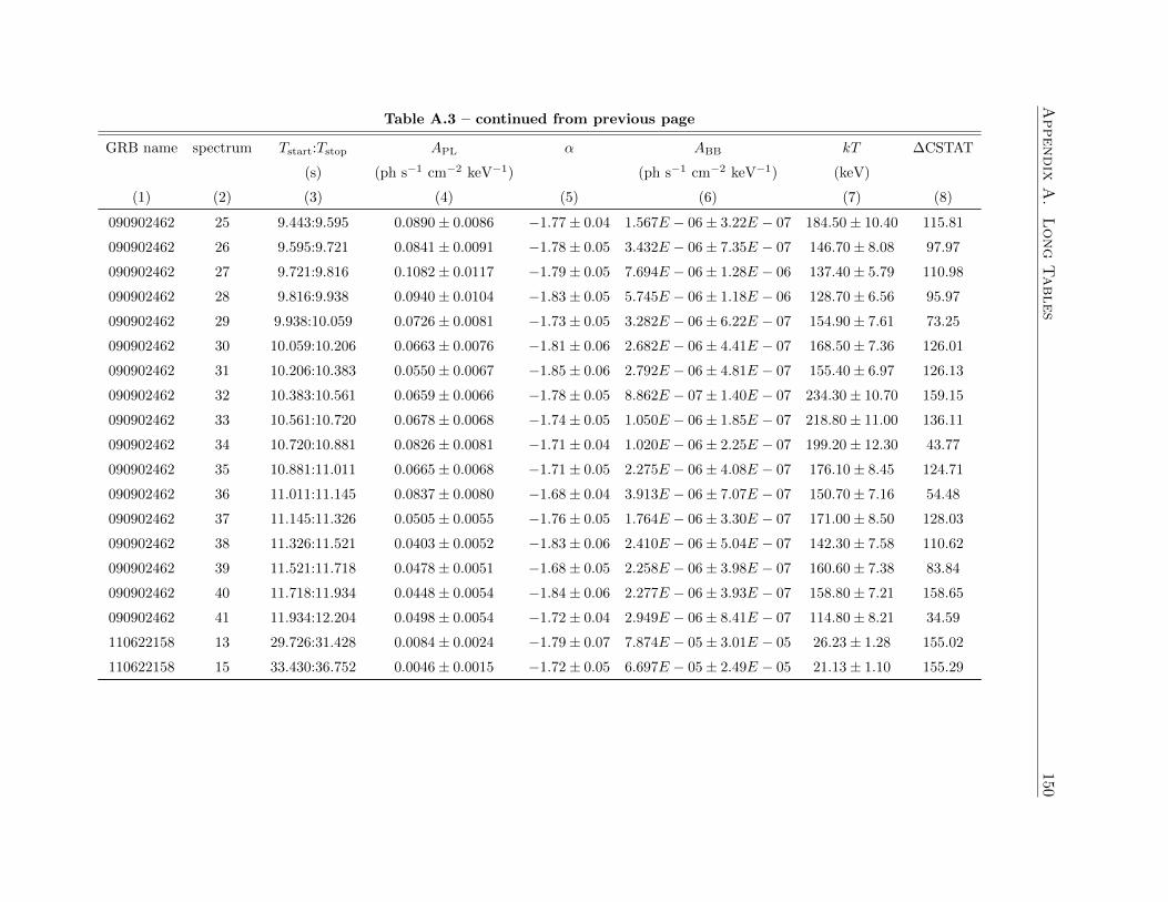
Appendix
A.
Long
Tables
150Table A.3 – continued from previous page
GRB name spectrum Tstart:Tstop APL α ABB kT ∆CSTAT
(s) (ph s−1 cm−2 keV−1) (ph s−1 cm−2 keV−1) (keV)
(1) (2) (3) (4) (5) (6) (7) (8)
090902462 25 9.443:9.595 0.0890± 0.0086 −1.77± 0.04 1.567E − 06± 3.22E − 07 184.50± 10.40 115.81
090902462 26 9.595:9.721 0.0841± 0.0091 −1.78± 0.05 3.432E − 06± 7.35E − 07 146.70± 8.08 97.97
090902462 27 9.721:9.816 0.1082± 0.0117 −1.79± 0.05 7.694E − 06± 1.28E − 06 137.40± 5.79 110.98
090902462 28 9.816:9.938 0.0940± 0.0104 −1.83± 0.05 5.745E − 06± 1.18E − 06 128.70± 6.56 95.97
090902462 29 9.938:10.059 0.0726± 0.0081 −1.73± 0.05 3.282E − 06± 6.22E − 07 154.90± 7.61 73.25
090902462 30 10.059:10.206 0.0663± 0.0076 −1.81± 0.06 2.682E − 06± 4.41E − 07 168.50± 7.36 126.01
090902462 31 10.206:10.383 0.0550± 0.0067 −1.85± 0.06 2.792E − 06± 4.81E − 07 155.40± 6.97 126.13
090902462 32 10.383:10.561 0.0659± 0.0066 −1.78± 0.05 8.862E − 07± 1.40E − 07 234.30± 10.70 159.15
090902462 33 10.561:10.720 0.0678± 0.0068 −1.74± 0.05 1.050E − 06± 1.85E − 07 218.80± 11.00 136.11
090902462 34 10.720:10.881 0.0826± 0.0081 −1.71± 0.04 1.020E − 06± 2.25E − 07 199.20± 12.30 43.77
090902462 35 10.881:11.011 0.0665± 0.0068 −1.71± 0.05 2.275E − 06± 4.08E − 07 176.10± 8.45 124.71
090902462 36 11.011:11.145 0.0837± 0.0080 −1.68± 0.04 3.913E − 06± 7.07E − 07 150.70± 7.16 54.48
090902462 37 11.145:11.326 0.0505± 0.0055 −1.76± 0.05 1.764E − 06± 3.30E − 07 171.00± 8.50 128.03
090902462 38 11.326:11.521 0.0403± 0.0052 −1.83± 0.06 2.410E − 06± 5.04E − 07 142.30± 7.58 110.62
090902462 39 11.521:11.718 0.0478± 0.0051 −1.68± 0.05 2.258E − 06± 3.98E − 07 160.60± 7.38 83.84
090902462 40 11.718:11.934 0.0448± 0.0054 −1.84± 0.06 2.277E − 06± 3.93E − 07 158.80± 7.21 158.65
090902462 41 11.934:12.204 0.0498± 0.0054 −1.72± 0.04 2.949E − 06± 8.41E − 07 114.80± 8.21 34.59
110622158 13 29.726:31.428 0.0084± 0.0024 −1.79± 0.07 7.874E − 05± 3.01E − 05 26.23± 1.28 155.02
110622158 15 33.430:36.752 0.0046± 0.0015 −1.72± 0.05 6.697E − 05± 2.49E − 05 21.13± 1.10 155.29
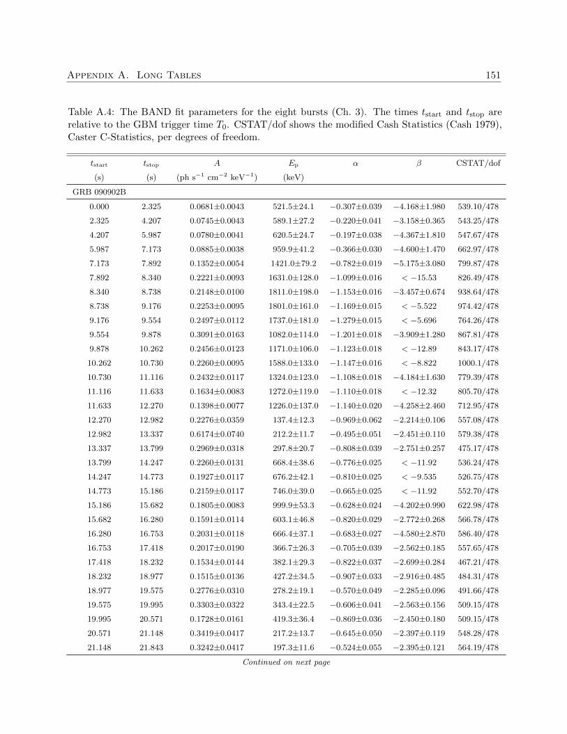
Appendix A. Long Tables 151
Table A.4: The BAND fit parameters for the eight bursts (Ch. 3). The times tstart and tstop arerelative to the GBM trigger time T0. CSTAT/dof shows the modified Cash Statistics (Cash 1979),Caster C-Statistics, per degrees of freedom.
tstart tstop A Ep α β CSTAT/dof
(s) (s) (ph s−1 cm−2 keV−1) (keV)
GRB 090902B
0.000 2.325 0.0681±0.0043 521.5±24.1 −0.307±0.039 −4.168±1.980 539.10/478
2.325 4.207 0.0745±0.0043 589.1±27.2 −0.220±0.041 −3.158±0.365 543.25/478
4.207 5.987 0.0780±0.0041 620.5±24.7 −0.197±0.038 −4.367±1.810 547.67/478
5.987 7.173 0.0885±0.0038 959.9±41.2 −0.366±0.030 −4.600±1.470 662.97/478
7.173 7.892 0.1352±0.0054 1421.0±79.2 −0.782±0.019 −5.175±3.080 799.87/478
7.892 8.340 0.2221±0.0093 1631.0±128.0 −1.099±0.016 < −15.53 826.49/478
8.340 8.738 0.2148±0.0100 1811.0±198.0 −1.153±0.016 −3.457±0.674 938.64/478
8.738 9.176 0.2253±0.0095 1801.0±161.0 −1.169±0.015 < −5.522 974.42/478
9.176 9.554 0.2497±0.0112 1737.0±181.0 −1.279±0.015 < −5.696 764.26/478
9.554 9.878 0.3091±0.0163 1082.0±114.0 −1.201±0.018 −3.909±1.280 867.81/478
9.878 10.262 0.2456±0.0123 1171.0±106.0 −1.123±0.018 < −12.89 843.17/478
10.262 10.730 0.2260±0.0095 1588.0±133.0 −1.147±0.016 < −8.822 1000.1/478
10.730 11.116 0.2432±0.0117 1324.0±123.0 −1.108±0.018 −4.184±1.630 779.39/478
11.116 11.633 0.1634±0.0083 1272.0±119.0 −1.110±0.018 < −12.32 805.70/478
11.633 12.270 0.1398±0.0077 1226.0±137.0 −1.140±0.020 −4.258±2.460 712.95/478
12.270 12.982 0.2276±0.0359 137.4±12.3 −0.969±0.062 −2.214±0.106 557.08/478
12.982 13.337 0.6174±0.0740 212.2±11.7 −0.495±0.051 −2.451±0.110 579.38/478
13.337 13.799 0.2969±0.0318 297.8±20.7 −0.808±0.039 −2.751±0.257 475.17/478
13.799 14.247 0.2260±0.0131 668.4±38.6 −0.776±0.025 < −11.92 536.24/478
14.247 14.773 0.1927±0.0117 676.2±42.1 −0.810±0.025 < −9.535 526.75/478
14.773 15.186 0.2159±0.0117 746.0±39.0 −0.665±0.025 < −11.92 552.70/478
15.186 15.682 0.1805±0.0083 999.9±53.3 −0.628±0.024 −4.202±0.990 622.98/478
15.682 16.280 0.1591±0.0114 603.1±46.8 −0.820±0.029 −2.772±0.268 566.78/478
16.280 16.753 0.2031±0.0118 666.4±37.1 −0.683±0.027 −4.580±2.870 586.40/478
16.753 17.418 0.2017±0.0190 366.7±26.3 −0.705±0.039 −2.562±0.185 557.65/478
17.418 18.232 0.1534±0.0144 382.1±29.3 −0.822±0.037 −2.699±0.284 467.21/478
18.232 18.977 0.1515±0.0136 427.2±34.5 −0.907±0.033 −2.916±0.485 484.31/478
18.977 19.575 0.2776±0.0310 278.2±19.1 −0.570±0.049 −2.285±0.096 491.66/478
19.575 19.995 0.3303±0.0322 343.4±22.5 −0.606±0.041 −2.563±0.156 509.15/478
19.995 20.571 0.1728±0.0161 419.3±36.4 −0.869±0.036 −2.450±0.180 509.15/478
20.571 21.148 0.3419±0.0417 217.2±13.7 −0.645±0.050 −2.397±0.119 548.28/478
21.148 21.843 0.3242±0.0417 197.3±11.6 −0.524±0.055 −2.395±0.121 564.19/478
Continued on next page
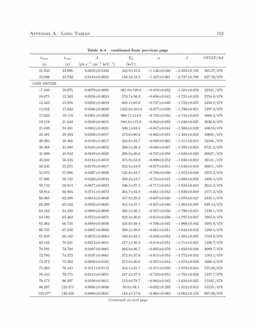
Appendix A. Long Tables 152
Table A.4 – continued from previous page
tstart tstop A Ep α β CSTAT/dof
(s) (s) (ph s−1 cm−2 keV−1) (keV)
21.843 23.098 0.0832±0.0103 342.9±45.0 −1.146±0.040 −2.283±0.192 565.37/478
23.098 33.792 0.0184±0.0055 134.3±19.5 −1.427±0.061 −2.727±0.780 627.70/478
GRB 100724B
-7.168 10.075 0.0079±0.0005 961.0±129.0 −0.878±0.032 −1.581±0.032 22341./478
10.075 12.503 0.0358±0.0024 570.7±56.3 −0.698±0.043 −1.721±0.035 2558.6/478
12.503 15.016 0.0292±0.0019 662.1±65.9 −0.727±0.040 −1.722±0.037 2459.2/478
15.016 17.022 0.0306±0.0020 1222.0±161.0 −0.877±0.030 −1.790±0.051 1297.9/478
17.022 19.118 0.0301±0.0020 968.7±114.0 −0.793±0.034 −1.744±0.043 1608.2/478
19.118 21.649 0.0249±0.0015 940.3±115.0 −0.882±0.033 −1.648±0.035 3636.6/478
21.649 24.481 0.0262±0.0021 580.1±83.4 −0.847±0.044 −1.580±0.029 4363.6/478
24.481 29.293 0.0208±0.0017 473.6±80.8 −0.862±0.051 −1.494±0.022 10681./478
29.293 38.468 0.0150±0.0017 282.6±49.7 −0.888±0.065 −1.511±0.015 53566./478
38.468 41.089 0.0445±0.0052 286.5±38.3 −0.688±0.067 −1.595±0.024 6721.3/478
41.089 45.942 0.0249±0.0025 298.9±36.6 −0.787±0.058 −1.628±0.020 20827./478
45.942 50.235 0.0184±0.0018 375.9±52.8 −0.890±0.052 −1.636±0.022 20121./478
50.235 55.075 0.0179±0.0017 352.5±44.9 −0.877±0.051 −1.646±0.019 20911./478
55.075 57.006 0.0397±0.0030 525.8±43.7 −0.780±0.039 −1.872±0.030 2355.2/478
57.006 58.742 0.0420±0.0034 499.2±43.7 −0.754±0.041 −1.888±0.028 3499.4/478
58.742 59.914 0.0677±0.0053 436.5±37.5 −0.717±0.044 −1.934±0.043 2615.2/478
59.914 60.965 0.0751±0.0072 364.7±34.8 −0.661±0.052 −1.936±0.049 2171.3/478
60.965 62.298 0.0613±0.0040 457.8±29.2 −0.687±0.040 −1.978±0.021 2335.1/478
62.298 63.162 0.0950±0.0095 454.5±47.1 −0.657±0.048 −1.903±0.050 829.13/478
63.162 64.192 0.0869±0.0099 368.5±38.1 −0.587±0.056 −1.796±0.031 1239.1/478
64.192 65.463 0.0752±0.0075 323.4±30.0 −0.615±0.056 −1.797±0.027 1907.0/478
65.463 66.735 0.0689±0.0056 434.0±39.4 −0.706±0.045 −1.906±0.042 1695.8/478
66.735 67.858 0.0807±0.0082 389.2±38.6 −0.661±0.051 −1.844±0.032 1289.5/478
67.858 69.182 0.0672±0.0064 349.3±32.5 −0.649±0.053 −1.805±0.025 1703.0/478
69.182 70.591 0.0474±0.0051 417.1±56.2 −0.819±0.051 −1.714±0.031 1498.7/478
70.591 72.794 0.0487±0.0061 262.8±30.7 −0.605±0.070 −1.650±0.026 3089.7/478
72.794 74.372 0.0597±0.0061 372.9±37.6 −0.615±0.054 −1.772±0.032 1165.1/478
74.372 75.362 0.0950±0.0105 373.0±36.6 −0.587±0.054 −1.874±0.038 1090.3/478
75.362 76.443 0.1011±0.0112 334.1±31.7 −0.571±0.056 −1.879±0.044 725.08/478
76.443 78.171 0.0513±0.0051 347.2±37.5 −0.759±0.053 −1.791±0.029 1247.7/478
78.171 86.297 0.0109±0.0011 513.8±78.7 −0.982±0.043 −1.634±0.025 15102./478
86.297 123.477 0.0056±0.0038 93.0±49.1 −0.692±0.292 −1.312±0.015 15525./478
123.477 130.458 0.0080±0.0041 143.4±17.6 −0.864±0.083 −2.062±0.134 907.00/478
Continued on next page
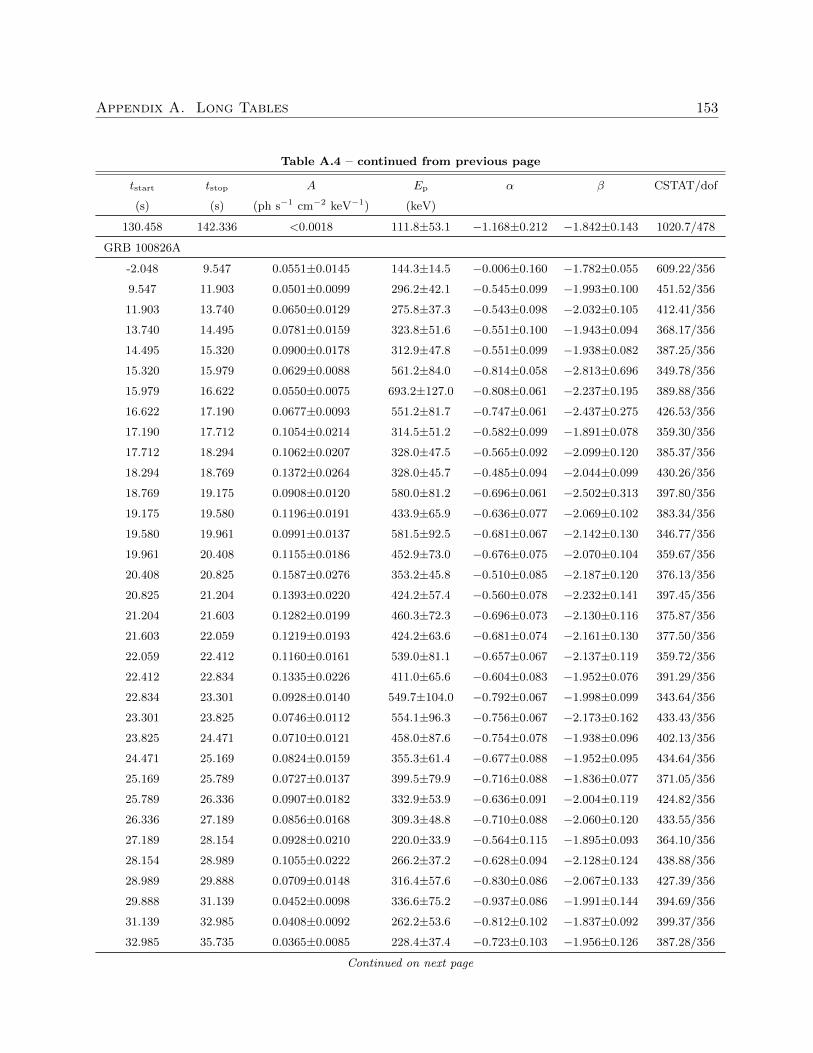
Appendix A. Long Tables 153
Table A.4 – continued from previous page
tstart tstop A Ep α β CSTAT/dof
(s) (s) (ph s−1 cm−2 keV−1) (keV)
130.458 142.336 <0.0018 111.8±53.1 −1.168±0.212 −1.842±0.143 1020.7/478
GRB 100826A
-2.048 9.547 0.0551±0.0145 144.3±14.5 −0.006±0.160 −1.782±0.055 609.22/356
9.547 11.903 0.0501±0.0099 296.2±42.1 −0.545±0.099 −1.993±0.100 451.52/356
11.903 13.740 0.0650±0.0129 275.8±37.3 −0.543±0.098 −2.032±0.105 412.41/356
13.740 14.495 0.0781±0.0159 323.8±51.6 −0.551±0.100 −1.943±0.094 368.17/356
14.495 15.320 0.0900±0.0178 312.9±47.8 −0.551±0.099 −1.938±0.082 387.25/356
15.320 15.979 0.0629±0.0088 561.2±84.0 −0.814±0.058 −2.813±0.696 349.78/356
15.979 16.622 0.0550±0.0075 693.2±127.0 −0.808±0.061 −2.237±0.195 389.88/356
16.622 17.190 0.0677±0.0093 551.2±81.7 −0.747±0.061 −2.437±0.275 426.53/356
17.190 17.712 0.1054±0.0214 314.5±51.2 −0.582±0.099 −1.891±0.078 359.30/356
17.712 18.294 0.1062±0.0207 328.0±47.5 −0.565±0.092 −2.099±0.120 385.37/356
18.294 18.769 0.1372±0.0264 328.0±45.7 −0.485±0.094 −2.044±0.099 430.26/356
18.769 19.175 0.0908±0.0120 580.0±81.2 −0.696±0.061 −2.502±0.313 397.80/356
19.175 19.580 0.1196±0.0191 433.9±65.9 −0.636±0.077 −2.069±0.102 383.34/356
19.580 19.961 0.0991±0.0137 581.5±92.5 −0.681±0.067 −2.142±0.130 346.77/356
19.961 20.408 0.1155±0.0186 452.9±73.0 −0.676±0.075 −2.070±0.104 359.67/356
20.408 20.825 0.1587±0.0276 353.2±45.8 −0.510±0.085 −2.187±0.120 376.13/356
20.825 21.204 0.1393±0.0220 424.2±57.4 −0.560±0.078 −2.232±0.141 397.45/356
21.204 21.603 0.1282±0.0199 460.3±72.3 −0.696±0.073 −2.130±0.116 375.87/356
21.603 22.059 0.1219±0.0193 424.2±63.6 −0.681±0.074 −2.161±0.130 377.50/356
22.059 22.412 0.1160±0.0161 539.0±81.1 −0.657±0.067 −2.137±0.119 359.72/356
22.412 22.834 0.1335±0.0226 411.0±65.6 −0.604±0.083 −1.952±0.076 391.29/356
22.834 23.301 0.0928±0.0140 549.7±104.0 −0.792±0.067 −1.998±0.099 343.64/356
23.301 23.825 0.0746±0.0112 554.1±96.3 −0.756±0.067 −2.173±0.162 433.43/356
23.825 24.471 0.0710±0.0121 458.0±87.6 −0.754±0.078 −1.938±0.096 402.13/356
24.471 25.169 0.0824±0.0159 355.3±61.4 −0.677±0.088 −1.952±0.095 434.64/356
25.169 25.789 0.0727±0.0137 399.5±79.9 −0.716±0.088 −1.836±0.077 371.05/356
25.789 26.336 0.0907±0.0182 332.9±53.9 −0.636±0.091 −2.004±0.119 424.82/356
26.336 27.189 0.0856±0.0168 309.3±48.8 −0.710±0.088 −2.060±0.120 433.55/356
27.189 28.154 0.0928±0.0210 220.0±33.9 −0.564±0.115 −1.895±0.093 364.10/356
28.154 28.989 0.1055±0.0222 266.2±37.2 −0.628±0.094 −2.128±0.124 438.88/356
28.989 29.888 0.0709±0.0148 316.4±57.6 −0.830±0.086 −2.067±0.133 427.39/356
29.888 31.139 0.0452±0.0098 336.6±75.2 −0.937±0.086 −1.991±0.144 394.69/356
31.139 32.985 0.0408±0.0092 262.2±53.6 −0.812±0.102 −1.837±0.092 399.37/356
32.985 35.735 0.0365±0.0085 228.4±37.4 −0.723±0.103 −1.956±0.126 387.28/356
Continued on next page
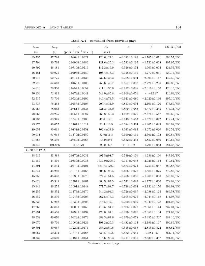
Appendix A. Long Tables 154
Table A.4 – continued from previous page
tstart tstop A Ep α β CSTAT/dof
(s) (s) (ph s−1 cm−2 keV−1) (keV)
35.735 37.794 0.0868±0.0321 126.6±21.1 −0.321±0.199 −1.765±0.071 393.57/356
37.794 40.792 0.0496±0.0189 121.6±25.3 −0.542±0.195 −1.722±0.068 407.95/356
40.792 46.181 0.0710±0.0216 117.2±15.9 −0.526±0.154 −1.963±0.094 424.55/356
46.181 60.975 0.0493±0.0150 108.4±13.3 −0.328±0.159 −1.777±0.051 520.17/356
60.975 62.775 0.0614±0.0135 232.6±35.3 −0.768±0.094 −2.094±0.147 442.50/356
62.775 64.610 0.0456±0.0105 258.6±45.7 −0.951±0.082 −2.221±0.236 402.38/356
64.610 70.330 0.0254±0.0057 211.1±35.6 −0.917±0.088 −2.016±0.150 426.15/356
70.330 72.515 0.0279±0.0041 549.0±85.8 −0.968±0.051 < −12.27 410.69/356
72.515 73.736 0.0520±0.0106 346.4±73.5 −0.941±0.080 −2.020±0.136 395.10/356
73.736 76.263 0.0455±0.0106 209.4±31.9 −0.813±0.094 −2.101±0.170 375.69/356
76.263 78.063 0.0561±0.0134 231.3±34.0 −0.889±0.083 −2.472±0.365 377.34/356
78.063 80.235 0.0354±0.0087 263.8±56.3 −1.199±0.070 −2.476±0.547 392.60/356
80.235 83.975 0.1548±0.2100 45.8±12.1 −0.143±0.553 −1.672±0.042 412.44/356
83.975 89.057 0.1167±0.1011 51.3±10.5 −0.384±0.364 −1.805±0.049 386.98/356
89.057 90.011 0.0838±0.0258 169.4±21.9 −1.043±0.082 −3.072±1.090 380.52/356
90.011 91.665 0.1179±0.0450 82.9±11.8 −0.950±0.151 −2.301±0.192 400.87/356
91.665 98.549 0.0659±0.0566 46.9±9.6 −0.552±0.343 −1.857±0.050 440.67/356
98.549 121.856 <1.5170 29.0±6.8 < −1.102 −1.791±0.053 581.38/356
GRB 101123A
38.912 43.589 0.0179±0.0033 497.5±98.7 −0.549±0.101 −1.926±0.100 447.95/356
43.589 44.391 0.0380±0.0033 1635.0±295.0 −0.717±0.048 −2.026±0.114 370.62/356
44.391 44.844 0.0770±0.0104 683.7±129.0 −0.583±0.073 −1.753±0.057 380.88/356
44.844 45.250 0.1016±0.0166 506.6±90.5 −0.606±0.077 −1.884±0.075 372.85/356
45.250 45.628 0.1530±0.0276 374.4±54.5 −0.486±0.088 −1.989±0.086 345.89/356
45.628 45.949 0.1407±0.0267 380.9±67.5 −0.541±0.093 −1.777±0.060 372.09/356
45.949 46.255 0.1001±0.0148 577.7±98.7 −0.728±0.064 −2.132±0.150 399.98/356
46.255 46.552 0.1173±0.0179 544.2±94.3 −0.726±0.067 −2.088±0.125 366.58/356
46.552 46.836 0.1243±0.0206 467.8±75.3 −0.605±0.076 −2.044±0.118 414.08/356
46.836 47.262 0.1339±0.0303 278.5±47.1 −0.702±0.095 −2.040±0.128 404.28/356
47.262 47.831 0.0808±0.0155 416.5±84.7 −0.825±0.077 −2.061±0.144 337.31/356
47.831 48.538 0.0739±0.0137 423.0±84.1 −0.826±0.076 −2.059±0.134 374.63/356
48.538 49.070 0.0923±0.0173 388.3±61.6 −0.679±0.078 −2.255±0.207 382.10/356
49.070 49.701 0.1666±0.0424 198.2±25.3 −0.482±0.114 −2.196±0.167 396.86/356
49.701 50.067 0.1229±0.0174 453.2±50.6 −0.515±0.068 −2.815±0.522 368.62/356
50.067 50.332 0.1673±0.0188 533.5±49.6 −0.582±0.055 −3.884±2.3 364.11/356
50.332 50.600 0.1184±0.0151 616.6±83.3 −0.711±0.056 −2.630±0.367 394.00/356
Continued on next page
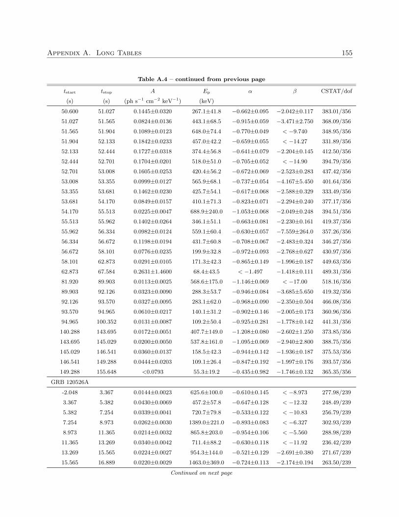
Appendix A. Long Tables 155
Table A.4 – continued from previous page
tstart tstop A Ep α β CSTAT/dof
(s) (s) (ph s−1 cm−2 keV−1) (keV)
50.600 51.027 0.1445±0.0320 267.1±41.8 −0.662±0.095 −2.042±0.117 383.01/356
51.027 51.565 0.0824±0.0136 443.1±68.5 −0.915±0.059 −3.471±2.750 368.09/356
51.565 51.904 0.1089±0.0123 648.0±74.4 −0.770±0.049 < −9.740 348.95/356
51.904 52.133 0.1842±0.0233 457.0±42.2 −0.659±0.055 < −14.27 331.89/356
52.133 52.444 0.1727±0.0318 374.4±56.8 −0.641±0.079 −2.204±0.145 412.50/356
52.444 52.701 0.1704±0.0201 518.0±51.0 −0.705±0.052 < −14.90 394.79/356
52.701 53.008 0.1605±0.0253 420.4±56.2 −0.672±0.069 −2.523±0.283 437.42/356
53.008 53.355 0.0999±0.0127 565.9±68.1 −0.737±0.054 −4.167±5.450 401.64/356
53.355 53.681 0.1462±0.0230 425.7±54.1 −0.617±0.068 −2.588±0.329 333.49/356
53.681 54.170 0.0849±0.0157 410.1±71.3 −0.823±0.071 −2.294±0.240 377.17/356
54.170 55.513 0.0225±0.0047 688.9±240.0 −1.053±0.068 −2.049±0.248 394.51/356
55.513 55.962 0.1402±0.0264 346.1±51.1 −0.663±0.081 −2.230±0.161 419.37/356
55.962 56.334 0.0982±0.0124 559.1±60.4 −0.630±0.057 −7.559±264.0 357.26/356
56.334 56.672 0.1198±0.0194 431.7±60.8 −0.708±0.067 −2.483±0.324 346.27/356
56.672 58.101 0.0776±0.0235 199.9±32.8 −0.972±0.093 −2.768±0.627 430.97/356
58.101 62.873 0.0291±0.0105 171.3±42.3 −0.865±0.149 −1.996±0.187 449.63/356
62.873 67.584 0.2631±1.4600 68.4±43.5 < −1.497 −1.418±0.111 489.31/356
81.920 89.903 0.0113±0.0025 568.6±175.0 −1.146±0.069 < −17.00 518.16/356
89.903 92.126 0.0323±0.0090 288.3±53.7 −0.946±0.084 −3.685±5.650 419.32/356
92.126 93.570 0.0327±0.0095 283.1±62.0 −0.968±0.090 −2.350±0.504 466.08/356
93.570 94.965 0.0610±0.0217 140.1±31.2 −0.902±0.146 −2.005±0.173 360.96/356
94.965 100.352 0.0131±0.0087 109.2±50.4 −0.925±0.281 −1.778±0.142 441.31/356
140.288 143.695 0.0172±0.0051 407.7±149.0 −1.208±0.080 −2.602±1.250 373.85/356
143.695 145.029 0.0200±0.0050 537.8±161.0 −1.095±0.069 −2.940±2.800 388.75/356
145.029 146.541 0.0360±0.0137 158.5±42.3 −0.944±0.142 −1.936±0.187 375.53/356
146.541 149.288 0.0444±0.0203 109.1±26.4 −0.847±0.192 −1.997±0.176 393.57/356
149.288 155.648 <0.0793 55.3±19.2 −0.435±0.982 −1.746±0.132 365.35/356
GRB 120526A
-2.048 3.367 0.0144±0.0023 625.6±100.0 −0.610±0.145 < −8.973 277.98/239
3.367 5.382 0.0430±0.0069 457.2±57.8 −0.647±0.128 < −12.32 248.49/239
5.382 7.254 0.0339±0.0041 720.7±79.8 −0.533±0.122 < −10.83 256.79/239
7.254 8.973 0.0262±0.0030 1389.0±221.0 −0.893±0.083 < −6.327 302.93/239
8.973 11.365 0.0214±0.0032 865.8±203.0 −0.954±0.106 < −5.560 288.98/239
11.365 13.269 0.0340±0.0042 711.4±88.2 −0.630±0.118 < −11.92 236.42/239
13.269 15.565 0.0224±0.0027 954.3±144.0 −0.521±0.129 −2.691±0.380 271.67/239
15.565 16.889 0.0220±0.0029 1463.0±369.0 −0.724±0.113 −2.174±0.194 263.50/239
Continued on next page
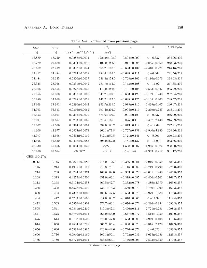
Appendix A. Long Tables 156
Table A.4 – continued from previous page
tstart tstop A Ep α β CSTAT/dof
(s) (s) (ph s−1 cm−2 keV−1) (keV)
16.889 18.729 0.0288±0.0034 1224.0±198.0 −0.894±0.090 < −6.337 264.96/239
18.729 20.182 0.0334±0.0042 1100.0±236.0 −0.911±0.098 −2.885±0.660 248.03/239
20.182 22.412 0.0302±0.0044 683.2±132.0 −0.693±0.134 −2.410±0.271 214.16/239
22.412 24.484 0.0214±0.0028 984.4±163.0 −0.698±0.117 < −6.364 241.56/239
24.484 26.325 0.0300±0.0037 936.3±158.0 −0.768±0.109 −3.186±0.976 234.93/239
26.325 28.016 0.0331±0.0042 781.7±114.0 −0.743±0.108 < −11.92 247.35/239
28.016 29.555 0.0278±0.0035 1119.0±238.0 −0.791±0.108 −2.533±0.347 285.22/239
29.555 30.980 0.0337±0.0052 640.2±109.0 −0.653±0.129 −3.159±1.240 257.64/239
30.980 33.168 0.0298±0.0039 746.7±117.0 −0.695±0.125 −3.105±0.903 285.57/239
33.168 34.993 0.0280±0.0042 853.7±219.0 −0.918±0.112 −2.499±0.407 246.47/239
34.993 36.553 0.0366±0.0062 697.4±204.0 −0.994±0.115 −2.269±0.253 255.41/239
36.553 37.691 0.0362±0.0079 475.6±109.0 −0.991±0.120 < −9.537 246.99/239
37.691 39.667 0.0253±0.0037 821.6±166.0 −0.825±0.115 −3.497±2.140 215.69/239
39.667 41.306 0.0374±0.0061 532.0±86.7 −0.813±0.119 < −14.64 242.91/239
41.306 42.977 0.0404±0.0074 466.1±77.8 −0.757±0.131 −3.940±4.880 204.96/239
42.977 44.596 0.0452±0.0110 342.3±56.5 −0.771±0.141 < −5.606 240.63/239
44.596 46.530 0.0407±0.0083 395.0±62.2 −0.781±0.132 < −14.90 253.36/239
46.530 56.166 0.0064±0.0047 <227.1 −1.568±0.307 −1.966±0.374 298.50/239
56.166 67.584 <0.0052 <21.2 < −1.847 −1.963±0.212 301.17/239
GRB 130427A
-0.064 0.145 0.0821±0.0080 1246.0±126.0 −0.386±0.081 −2.916±0.359 1489.3/357
0.145 0.214 0.1936±0.0197 918.8±73.1 −0.116±0.089 −3.719±0.799 1275.0/357
0.214 0.268 0.3744±0.0374 764.6±62.0 −0.363±0.074 −4.031±1.280 1246.8/357
0.268 0.313 0.4275±0.0506 657.9±63.1 −0.319±0.085 −3.400±0.702 1168.7/357
0.313 0.358 0.5104±0.0558 569.5±42.7 −0.332±0.078 −4.889±3.570 1163.6/357
0.358 0.398 0.4528±0.0510 734.1±75.3 −0.560±0.070 −3.750±1.090 1169.3/357
0.398 0.434 0.7357±0.1020 486.6±47.5 −0.593±0.075 −3.979±1.580 1115.3/357
0.434 0.472 0.5783±0.0660 617.0±60.7 −0.610±0.066 < −11.92 1119.4/357
0.472 0.505 0.5876±0.0804 572.7±69.1 −0.676±0.072 −3.286±0.834 1090.3/357
0.505 0.541 0.9841±0.2210 319.3±42.3 −0.466±0.111 −2.721±0.281 1098.2/357
0.541 0.575 0.6740±0.1011 465.0±53.0 −0.647±0.077 −3.512±1.050 1100.0/357
0.575 0.614 0.8132±0.1500 379.0±47.8 −0.593±0.089 −2.949±0.408 1113.6/357
0.614 0.656 0.4534±0.0718 505.2±65.4 −0.800±0.070 −3.815±2.120 1107.9/357
0.656 0.696 0.5599±0.0885 423.0±44.6 −0.726±0.072 < −6.620 1089.5/357
0.696 0.736 0.5940±0.1160 366.3±50.1 −0.762±0.087 −3.075±0.656 1123.8/357
0.736 0.780 0.4775±0.1011 383.8±65.1 −0.746±0.095 −2.593±0.350 1170.2/357
Continued on next page
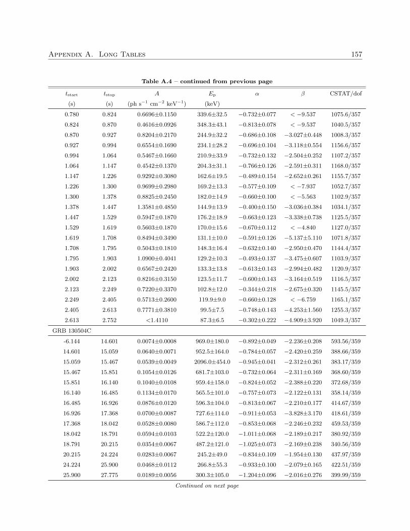
Appendix A. Long Tables 157
Table A.4 – continued from previous page
tstart tstop A Ep α β CSTAT/dof
(s) (s) (ph s−1 cm−2 keV−1) (keV)
0.780 0.824 0.6696±0.1150 339.6±32.5 −0.732±0.077 < −9.537 1075.6/357
0.824 0.870 0.4616±0.0926 348.3±43.1 −0.813±0.078 < −9.537 1040.5/357
0.870 0.927 0.8204±0.2170 244.9±32.2 −0.686±0.108 −3.027±0.448 1008.3/357
0.927 0.994 0.6554±0.1690 234.1±28.2 −0.696±0.104 −3.118±0.554 1156.6/357
0.994 1.064 0.5467±0.1660 210.9±33.9 −0.732±0.132 −2.504±0.252 1107.2/357
1.064 1.147 0.4542±0.1370 204.3±31.1 −0.766±0.126 −2.591±0.311 1168.0/357
1.147 1.226 0.9292±0.3080 162.6±19.5 −0.489±0.154 −2.652±0.261 1155.7/357
1.226 1.300 0.9699±0.2980 169.2±13.3 −0.577±0.109 < −7.937 1052.7/357
1.300 1.378 0.8825±0.2450 182.0±14.9 −0.660±0.100 < −5.563 1102.9/357
1.378 1.447 1.3581±0.4850 144.9±13.9 −0.400±0.150 −3.036±0.384 1034.1/357
1.447 1.529 0.5947±0.1870 176.2±18.9 −0.663±0.123 −3.338±0.738 1125.5/357
1.529 1.619 0.5603±0.1870 170.0±15.6 −0.670±0.112 < −4.840 1127.0/357
1.619 1.708 0.8494±0.3490 131.1±10.0 −0.591±0.126 −5.137±5.110 1071.8/357
1.708 1.795 0.5043±0.1810 148.3±16.4 −0.632±0.140 −2.950±0.470 1144.4/357
1.795 1.903 1.0900±0.4041 129.2±10.3 −0.493±0.137 −3.475±0.607 1103.9/357
1.903 2.002 0.6567±0.2420 133.3±13.8 −0.613±0.143 −2.994±0.482 1120.9/357
2.002 2.123 0.8216±0.3150 123.5±11.7 −0.600±0.143 −3.164±0.519 1116.5/357
2.123 2.249 0.7220±0.3370 102.8±12.0 −0.344±0.218 −2.675±0.320 1145.5/357
2.249 2.405 0.5713±0.2600 119.9±9.0 −0.660±0.128 < −6.759 1165.1/357
2.405 2.613 0.7771±0.3810 99.5±7.5 −0.748±0.143 −4.253±1.560 1255.3/357
2.613 2.752 <1.4110 87.3±6.5 −0.302±0.222 −4.909±3.920 1049.3/357
GRB 130504C
-6.144 14.601 0.0074±0.0008 969.0±180.0 −0.892±0.049 −2.236±0.208 593.56/359
14.601 15.059 0.0640±0.0071 952.5±164.0 −0.784±0.057 −2.420±0.259 388.66/359
15.059 15.467 0.0539±0.0049 2096.0±454.0 −0.945±0.041 −2.312±0.261 383.17/359
15.467 15.851 0.1054±0.0126 681.7±103.0 −0.732±0.064 −2.311±0.169 368.60/359
15.851 16.140 0.1040±0.0108 959.4±158.0 −0.824±0.052 −2.388±0.220 372.68/359
16.140 16.485 0.1134±0.0170 565.5±101.0 −0.757±0.073 −2.122±0.131 358.14/359
16.485 16.926 0.0876±0.0120 596.3±104.0 −0.813±0.067 −2.210±0.177 414.67/359
16.926 17.368 0.0700±0.0087 727.6±114.0 −0.911±0.053 −3.828±3.170 418.61/359
17.368 18.042 0.0528±0.0080 586.7±112.0 −0.853±0.068 −2.246±0.232 459.53/359
18.042 18.791 0.0594±0.0103 522.2±120.0 −1.011±0.068 −2.189±0.217 380.92/359
18.791 20.215 0.0354±0.0067 487.2±121.0 −1.025±0.073 −2.169±0.238 340.56/359
20.215 24.224 0.0283±0.0067 245.2±49.0 −0.834±0.109 −1.954±0.130 437.97/359
24.224 25.900 0.0468±0.0112 266.8±55.3 −0.933±0.100 −2.079±0.165 422.51/359
25.900 27.775 0.0189±0.0056 300.3±105.0 −1.204±0.096 −2.016±0.276 399.99/359
Continued on next page
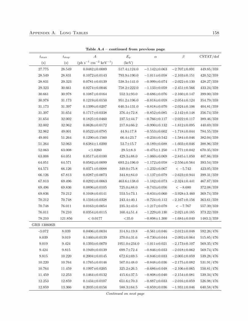
Appendix A. Long Tables 158
Table A.4 – continued from previous page
tstart tstop A Ep α β CSTAT/dof
(s) (s) (ph s−1 cm−2 keV−1) (keV)
27.775 28.549 0.0482±0.0089 517.4±124.0 −1.142±0.063 −2.707±0.891 449.85/359
28.549 28.831 0.1072±0.0143 793.9±190.0 −1.011±0.058 −2.103±0.151 420.52/359
28.831 29.323 0.0781±0.0139 538.3±141.0 −0.999±0.074 −2.022±0.130 428.27/359
29.323 30.661 0.0274±0.0046 758.2±222.0 −1.133±0.059 −2.451±0.566 433.24/359
30.661 30.978 0.1087±0.0164 552.3±93.0 −0.686±0.076 −2.160±0.147 399.00/359
30.978 31.173 0.1219±0.0150 951.2±196.0 −0.818±0.059 −2.054±0.124 354.79/359
31.173 31.397 0.1399±0.0207 640.3±131.0 −0.818±0.070 −2.024±0.106 404.81/359
31.397 31.654 0.1717±0.0338 376.4±72.8 −0.852±0.085 −2.142±0.148 356.74/359
31.654 32.002 0.1825±0.0460 237.5±44.7 −0.766±0.117 −2.022±0.117 389.46/359
32.002 32.962 0.0626±0.0172 217.8±66.2 −0.990±0.132 −1.812±0.095 440.69/359
32.962 49.001 0.0522±0.0785 44.9±17.8 −0.553±0.602 −1.718±0.044 784.55/359
49.001 51.264 0.1290±0.1560 66.4±23.7 −0.234±0.542 −1.584±0.046 382.04/359
51.264 52.063 0.6384±1.0200 53.7±15.7 −0.189±0.688 −1.603±0.046 388.96/359
52.063 63.008 <1.0260 29.5±8.3 −0.475±1.250 −1.771±0.042 670.35/359
63.008 64.051 0.0517±0.0100 429.3±88.0 −1.060±0.069 −2.845±1.050 407.86/359
64.051 64.571 0.0582±0.0099 693.2±196.0 −1.172±0.058 −2.556±0.564 393.54/359
64.571 66.126 0.0371±0.0088 349.0±75.8 −1.232±0.067 < −5.742 423.05/359
66.126 67.813 0.0287±0.0073 344.8±84.0 −1.137±0.079 −2.623±0.944 399.31/359
67.813 69.496 0.0292±0.0063 463.6±138.0 −1.182±0.073 −2.324±0.441 467.87/359
69.496 69.836 0.0896±0.0105 725.0±88.0 −0.743±0.056 < −8.680 372.08/359
69.836 70.212 0.1048±0.0141 553.5±73.1 −0.834±0.060 −3.928±3.460 369.74/359
70.212 70.748 0.1316±0.0328 243.4±40.1 −0.724±0.112 −2.167±0.156 363.61/359
70.748 76.011 0.0163±0.0054 235.3±43.6 −1.217±0.078 < −7.767 557.39/359
76.011 78.210 0.0354±0.0115 160.4±51.4 −1.229±0.130 −2.021±0.185 373.22/359
78.210 121.856 < 0.0177 <35.0 −0.898±1.300 −1.684±0.040 1483.3/359
GRB 130606B
-3.072 8.039 0.0406±0.0034 314.8±19.8 −0.561±0.046 −2.012±0.048 592.26/476
8.039 9.019 0.1460±0.0139 370.0±31.6 −0.730±0.044 −2.092±0.064 515.85/476
9.019 9.424 0.1393±0.0070 1951.0±234.0 −1.011±0.021 −2.173±0.107 569.35/476
9.424 9.815 0.1949±0.0139 699.7±72.4 −0.846±0.033 −2.018±0.062 569.74/476
9.815 10.220 0.2004±0.0145 672.6±69.5 −0.846±0.033 −2.005±0.059 539.28/476
10.220 10.764 0.1765±0.0146 507.0±48.0 −0.848±0.036 −2.175±0.082 531.91/476
10.764 11.459 0.1997±0.0205 325.2±26.5 −0.686±0.048 −2.106±0.065 550.81/476
11.459 12.253 0.1464±0.0132 415.6±37.5 −0.808±0.040 −2.154±0.081 539.34/476
12.253 12.859 0.1434±0.0107 651.6±70.3 −0.887±0.033 −2.016±0.059 526.98/476
12.859 13.366 0.2035±0.0156 588.3±64.5 −0.859±0.036 −1.931±0.046 640.58/476
Continued on next page
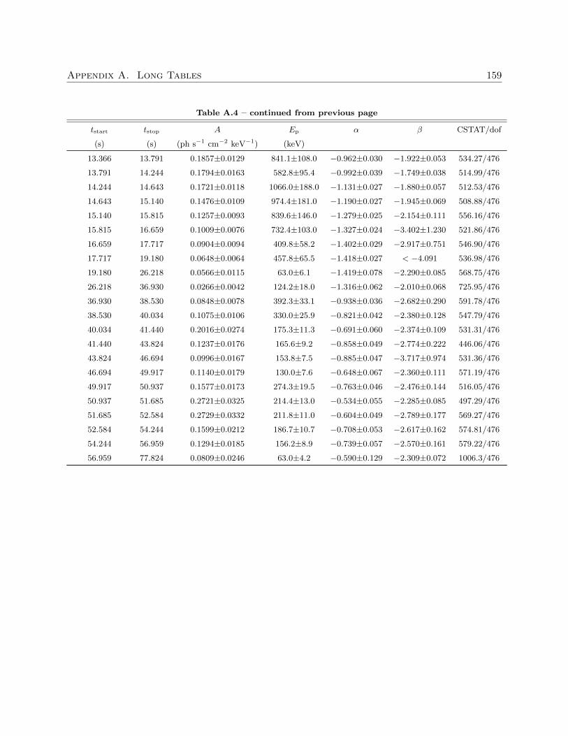
Appendix A. Long Tables 159
Table A.4 – continued from previous page
tstart tstop A Ep α β CSTAT/dof
(s) (s) (ph s−1 cm−2 keV−1) (keV)
13.366 13.791 0.1857±0.0129 841.1±108.0 −0.962±0.030 −1.922±0.053 534.27/476
13.791 14.244 0.1794±0.0163 582.8±95.4 −0.992±0.039 −1.749±0.038 514.99/476
14.244 14.643 0.1721±0.0118 1066.0±188.0 −1.131±0.027 −1.880±0.057 512.53/476
14.643 15.140 0.1476±0.0109 974.4±181.0 −1.190±0.027 −1.945±0.069 508.88/476
15.140 15.815 0.1257±0.0093 839.6±146.0 −1.279±0.025 −2.154±0.111 556.16/476
15.815 16.659 0.1009±0.0076 732.4±103.0 −1.327±0.024 −3.402±1.230 521.86/476
16.659 17.717 0.0904±0.0094 409.8±58.2 −1.402±0.029 −2.917±0.751 546.90/476
17.717 19.180 0.0648±0.0064 457.8±65.5 −1.418±0.027 < −4.091 536.98/476
19.180 26.218 0.0566±0.0115 63.0±6.1 −1.419±0.078 −2.290±0.085 568.75/476
26.218 36.930 0.0266±0.0042 124.2±18.0 −1.316±0.062 −2.010±0.068 725.95/476
36.930 38.530 0.0848±0.0078 392.3±33.1 −0.938±0.036 −2.682±0.290 591.78/476
38.530 40.034 0.1075±0.0106 330.0±25.9 −0.821±0.042 −2.380±0.128 547.79/476
40.034 41.440 0.2016±0.0274 175.3±11.3 −0.691±0.060 −2.374±0.109 531.31/476
41.440 43.824 0.1237±0.0176 165.6±9.2 −0.858±0.049 −2.774±0.222 446.06/476
43.824 46.694 0.0996±0.0167 153.8±7.5 −0.885±0.047 −3.717±0.974 531.36/476
46.694 49.917 0.1140±0.0179 130.0±7.6 −0.648±0.067 −2.360±0.111 571.19/476
49.917 50.937 0.1577±0.0173 274.3±19.5 −0.763±0.046 −2.476±0.144 516.05/476
50.937 51.685 0.2721±0.0325 214.4±13.0 −0.534±0.055 −2.285±0.085 497.29/476
51.685 52.584 0.2729±0.0332 211.8±11.0 −0.604±0.049 −2.789±0.177 569.27/476
52.584 54.244 0.1599±0.0212 186.7±10.7 −0.708±0.053 −2.617±0.162 574.81/476
54.244 56.959 0.1294±0.0185 156.2±8.9 −0.739±0.057 −2.570±0.161 579.22/476
56.959 77.824 0.0809±0.0246 63.0±4.2 −0.590±0.129 −2.309±0.072 1006.3/476
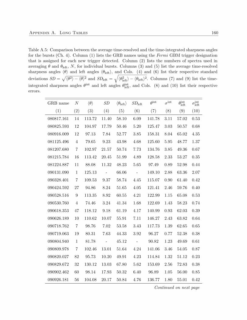
Appendix A. Long Tables 160
Table A.5: Comparison between the average time-resolved and the time-integrated sharpness anglesfor the bursts (Ch. 4). Column (1) lists the GRB names using the Fermi GBM trigger designationthat is assigned for each new trigger detected. Column (2) lists the numbers of spectra used inaveraging θ and θleft, N , for individual bursts. Columns (3) and (5) list the average time-resolvedsharpness angles 〈θ〉 and left angles 〈θleft〉, and Cols. (4) and (6) list their respective standard
deviations SD =√〈θ2〉 − 〈θ〉2 and SDleft =
√〈θ2
left〉 − 〈θleft〉2. Columns (7) and (9) list the time-
integrated sharpness angles θint and left angles θintleft, and Cols. (8) and (10) list their respective
errors.
GRB name N 〈θ〉 SD 〈θleft〉 SDleft θint σint θintleft σint
left
(1) (2) (3) (4) (5) (6) (7) (8) (9) (10)
080817.161 14 113.72 11.40 58.10 6.09 141.78 3.11 57.02 0.53
080825.593 12 104.97 17.79 50.46 5.20 125.47 3.03 50.57 0.68
080916.009 12 97.13 7.84 52.77 3.85 158.31 8.04 65.02 4.35
081125.496 4 79.65 9.23 43.98 4.68 125.60 5.95 48.77 1.37
081207.680 7 102.97 21.57 50.74 7.73 134.76 3.85 49.36 0.67
081215.784 16 113.42 20.45 51.99 4.89 128.58 2.33 53.27 0.35
081224.887 11 88.08 11.32 48.23 5.65 97.49 0.89 52.98 0.44
090131.090 1 125.13 - 66.06 - 149.10 2.88 63.36 2.07
090328.401 7 109.53 9.37 58.74 4.45 115.07 0.90 61.40 0.42
090424.592 27 94.86 8.24 51.65 4.05 121.41 2.46 59.76 0.40
090528.516 9 113.35 8.92 60.55 4.21 122.99 1.15 65.08 0.53
090530.760 4 74.46 3.24 41.34 1.68 122.69 1.43 58.23 0.74
090618.353 47 118.12 9.18 61.19 4.17 140.99 0.93 62.03 0.39
090626.189 10 110.62 10.07 55.91 7.11 146.27 2.43 63.82 0.64
090718.762 7 98.76 7.02 53.58 3.43 117.73 1.39 62.65 0.65
090719.063 19 80.31 7.63 44.33 3.92 96.27 0.77 52.38 0.38
090804.940 1 81.78 - 45.12 - 90.82 1.23 49.69 0.61
090809.978 7 102.46 13.01 51.64 4.24 141.06 3.46 54.05 0.87
090820.027 82 95.73 10.20 49.91 4.23 114.84 1.32 51.12 0.23
090829.672 32 130.12 13.03 67.80 5.62 153.69 2.56 72.83 0.38
090902.462 60 98.14 17.93 50.32 6.40 96.89 1.05 56.00 0.85
090926.181 56 104.08 20.17 50.84 4.76 136.77 1.80 55.01 0.42
Continued on next page
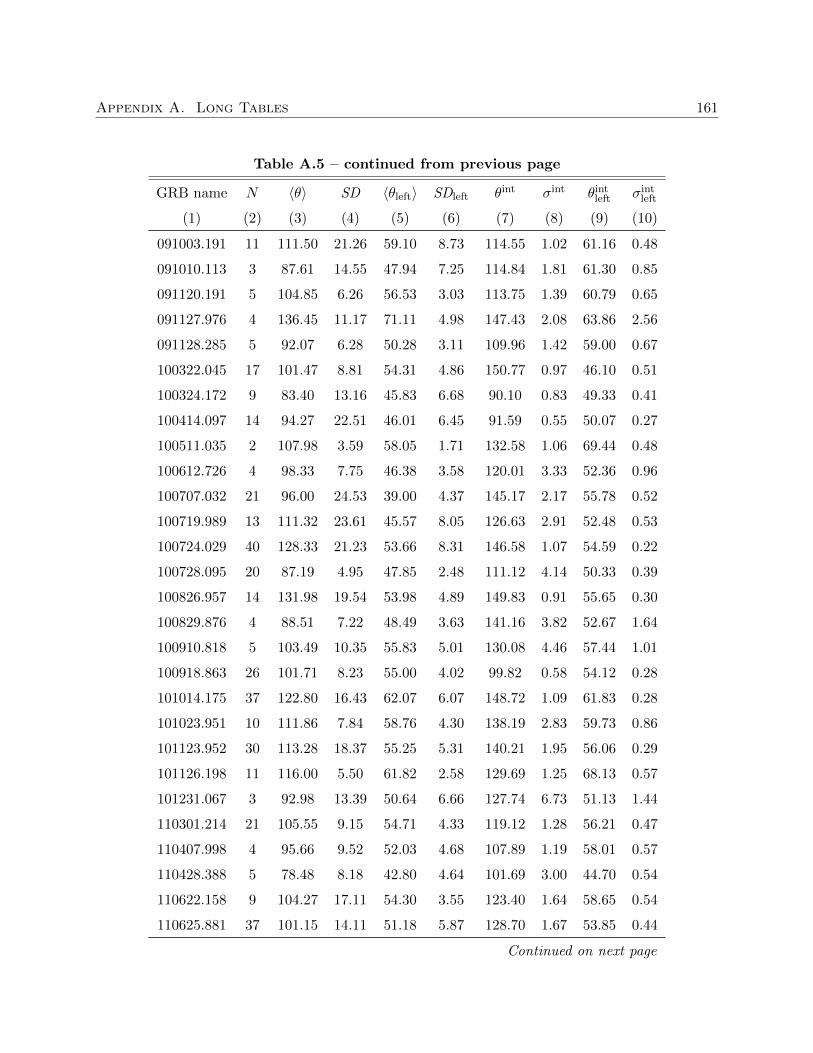
Appendix A. Long Tables 161
Table A.5 – continued from previous page
GRB name N 〈θ〉 SD 〈θleft〉 SDleft θint σint θintleft σint
left
(1) (2) (3) (4) (5) (6) (7) (8) (9) (10)
091003.191 11 111.50 21.26 59.10 8.73 114.55 1.02 61.16 0.48
091010.113 3 87.61 14.55 47.94 7.25 114.84 1.81 61.30 0.85
091120.191 5 104.85 6.26 56.53 3.03 113.75 1.39 60.79 0.65
091127.976 4 136.45 11.17 71.11 4.98 147.43 2.08 63.86 2.56
091128.285 5 92.07 6.28 50.28 3.11 109.96 1.42 59.00 0.67
100322.045 17 101.47 8.81 54.31 4.86 150.77 0.97 46.10 0.51
100324.172 9 83.40 13.16 45.83 6.68 90.10 0.83 49.33 0.41
100414.097 14 94.27 22.51 46.01 6.45 91.59 0.55 50.07 0.27
100511.035 2 107.98 3.59 58.05 1.71 132.58 1.06 69.44 0.48
100612.726 4 98.33 7.75 46.38 3.58 120.01 3.33 52.36 0.96
100707.032 21 96.00 24.53 39.00 4.37 145.17 2.17 55.78 0.52
100719.989 13 111.32 23.61 45.57 8.05 126.63 2.91 52.48 0.53
100724.029 40 128.33 21.23 53.66 8.31 146.58 1.07 54.59 0.22
100728.095 20 87.19 4.95 47.85 2.48 111.12 4.14 50.33 0.39
100826.957 14 131.98 19.54 53.98 4.89 149.83 0.91 55.65 0.30
100829.876 4 88.51 7.22 48.49 3.63 141.16 3.82 52.67 1.64
100910.818 5 103.49 10.35 55.83 5.01 130.08 4.46 57.44 1.01
100918.863 26 101.71 8.23 55.00 4.02 99.82 0.58 54.12 0.28
101014.175 37 122.80 16.43 62.07 6.07 148.72 1.09 61.83 0.28
101023.951 10 111.86 7.84 58.76 4.30 138.19 2.83 59.73 0.86
101123.952 30 113.28 18.37 55.25 5.31 140.21 1.95 56.06 0.29
101126.198 11 116.00 5.50 61.82 2.58 129.69 1.25 68.13 0.57
101231.067 3 92.98 13.39 50.64 6.66 127.74 6.73 51.13 1.44
110301.214 21 105.55 9.15 54.71 4.33 119.12 1.28 56.21 0.47
110407.998 4 95.66 9.52 52.03 4.68 107.89 1.19 58.01 0.57
110428.388 5 78.48 8.18 42.80 4.64 101.69 3.00 44.70 0.54
110622.158 9 104.27 17.11 54.30 3.55 123.40 1.64 58.65 0.54
110625.881 37 101.15 14.11 51.18 5.87 128.70 1.67 53.85 0.44
Continued on next page
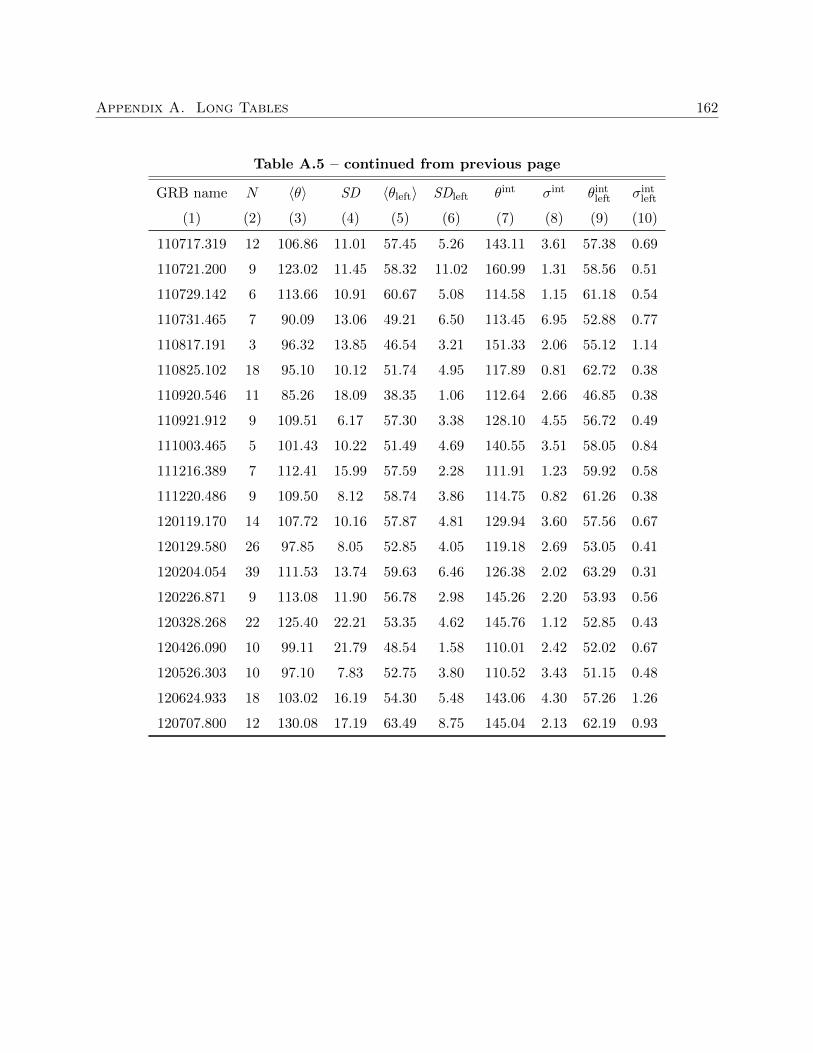
Appendix A. Long Tables 162
Table A.5 – continued from previous page
GRB name N 〈θ〉 SD 〈θleft〉 SDleft θint σint θintleft σint
left
(1) (2) (3) (4) (5) (6) (7) (8) (9) (10)
110717.319 12 106.86 11.01 57.45 5.26 143.11 3.61 57.38 0.69
110721.200 9 123.02 11.45 58.32 11.02 160.99 1.31 58.56 0.51
110729.142 6 113.66 10.91 60.67 5.08 114.58 1.15 61.18 0.54
110731.465 7 90.09 13.06 49.21 6.50 113.45 6.95 52.88 0.77
110817.191 3 96.32 13.85 46.54 3.21 151.33 2.06 55.12 1.14
110825.102 18 95.10 10.12 51.74 4.95 117.89 0.81 62.72 0.38
110920.546 11 85.26 18.09 38.35 1.06 112.64 2.66 46.85 0.38
110921.912 9 109.51 6.17 57.30 3.38 128.10 4.55 56.72 0.49
111003.465 5 101.43 10.22 51.49 4.69 140.55 3.51 58.05 0.84
111216.389 7 112.41 15.99 57.59 2.28 111.91 1.23 59.92 0.58
111220.486 9 109.50 8.12 58.74 3.86 114.75 0.82 61.26 0.38
120119.170 14 107.72 10.16 57.87 4.81 129.94 3.60 57.56 0.67
120129.580 26 97.85 8.05 52.85 4.05 119.18 2.69 53.05 0.41
120204.054 39 111.53 13.74 59.63 6.46 126.38 2.02 63.29 0.31
120226.871 9 113.08 11.90 56.78 2.98 145.26 2.20 53.93 0.56
120328.268 22 125.40 22.21 53.35 4.62 145.76 1.12 52.85 0.43
120426.090 10 99.11 21.79 48.54 1.58 110.01 2.42 52.02 0.67
120526.303 10 97.10 7.83 52.75 3.80 110.52 3.43 51.15 0.48
120624.933 18 103.02 16.19 54.30 5.48 143.06 4.30 57.26 1.26
120707.800 12 130.08 17.19 63.49 8.75 145.04 2.13 62.19 0.93