constraint network approach to the design and manufacture of labels in a high-variety label-printing...
TRANSCRIPT
Journal o f Intelligent Manufacturing (1996) 7, 499-514
Constraint network approach to the design and manufacture of labels in a high-variety label-printing environment
A. O. AWOFALA and N. SINGH*
Department of Industrial and Manufacturing Engineering, Wayne State University, Detroit, MI 48202, USA
Received October 1995 and accepted April 1996
This paper presents a constraint network approach to the design and manufacture of high-variety labels. The existing approach to label printing in the industry is essentially a sequential approach. In this approach, layout sheet utilization is optimized based on label attributes only. Production then attempts to meet delivery date of the labels by first processing high-priority labels from the layout sheet, and others later. This results in huge work-in-process inventory and high production cost. In this paper, we propose a constraint network approach to the design and manufacture of labels on layout sheets. Mathematical models of the various manufacturing stages are considered in the design process. Thus the emerging optimal layout design minimizes the work-in-process inventory and production cost, and maximizes production efficiency. The algorithm is an application of artificial intelligence techniques in a system domain. An example application of the algorithm results in an efficient production schedule and greater product delivery performance.
Keywords: Concurrent engineering, constraint network, cutting stocks, design and manufacturing
1. Introduction
Today's competitive market requires that manufacturing companies react quickly to volatile market demands and growing product complexity through efficient design processes that ensure a product's quality, competitive price, prompt availability, and delivery to consumers. Success stories (Ardayfio et al., 1992; Wheeler et al., 1991) have shown that this can be achieved by adopting a manufacturing philosophy termed concurrent engineering. Concurrent engineering (CE) is an approach in which all elements of a product life cycle, such as manufacturing, quality, assembly, inspection, repair and disposal, are considered at the design stage. Creese and Moore (1990) have defined CE as a management philosophy for improving quality, reducing costs and lead time from product conception to development for new products and product modifications. Researchers have focused on a variety of methods to reduce life-cycle costs and time-to- market of new products. A multifunctional team approach has been proposed in which experts in various phases of the product life cycle work together as a team to manage
*Author to whom all correspondence should be addressed.
0956-5515 © 1996 Chapman & Hall
all phases of the life cycle (Evans, 1988; Hartley, 1992; Turino, 1991). O'Grady et al. (O'Grady and Young, 1991; O'Grady et al., 1992; Fohn et al., 1994) developed a constraint network approach to concurrent engineering. In their approach, constraints are interconnected by virtue of sharing variables in a logical form. A set of variables that satisfy all constraints depicts a feasible solution. Okogbaa and Vaiyapuri (1993) describe a design approach by which the product design is decomposed to represent its basic functional features. Axiomatic design principles are used in identifying product features. Information sharing between design and manufacturing is based on finite element analysis techniques. In this paper, we apply the constraint network approach to a non-traditional area: the high-variety label-printing environment.
In this environment, labels are arranged on a large layout sheet to minimize the trim loss. The production of labels starts with an optical image copy of the label arrangement onto films to develop printing plates. The required quantity of sheets is printed using the printing plates, followed by jogging the printed sheets in blocks of 1000 sheets (jogging is the process of removing air between the layout sheets). The cutting department cuts individual labels from the block of sheets. The labels are
500 Awofala and Singh
packed into cartons and sealed. This environment has other objectives as well as minimizing trim loss, including satisfying customer due dates, improving production efficiency, and minimizing work-in-process inventory.
Most of the research work in this area has focused on the cutting stock problem (Golden, 1976; Albano and Sappupo, 1980; Agrawal, 1993; Arbel, 1993). The task is to find a way of cutting smaller order pieces from a large stock sheet that will minimize the trim loss. The broad applications in industry range from the stamping of metal plates from large sheet metal in stamping operations and boards in furniture building to the placement of sewing patterns on sheets of material.
Christofides and Whitlock (1977) presented a tree- search alogrithm, where each node on the tree repre- sented a cut. They placed the guillotine restriction upon the problem. A guillotine cut is one that is made from one edge of a rectangular sheet to the opposite edge. Using a branch-and-bound method, they were able to generate feasible cutting patterns.
Wang (1983) used a combinational algorithm to find guillotine cutting patterns by successively adding the rectangles to each other. Undesirable additions were rejected to reduce the number of such combinations by a choice of parameters.
Adamowicz and Albano (1986) used their observation that when an experienced person lays out rectangles on a sheet, he or she usually tries to group them into sets having at least one dimension in common. They called these sets 'strips', and avoided having exhaustive search procedures by generating these strips and employing a constrained dynamic programming algorithm to fill the sheet with them.
Israni and Sanders (1982) used a problem reduction algorithm that allows human intervention during the run to fill in possible resultant gaps. A simulation model to arrange lable patterns on a layout was developed by Bookbinder and Higginson (1986).
In the above methods, no consideration is given to important factors such as customer order due date, colour constraints, printing capacity constraints, or cutting capacity constraints, thus making the application of such approaches impractical. Singh and Wang (1994) investi- gated the interaction between layout design and manu- facture. The result of their work showed that the layout design affects cutting time as well as work-in-process inventory. A predictive equation was developed to determine the forecast cutting time as a function of the number of cuts and quantity of layout sheets. Their work focused on the cutting stage of the label production process while ignoring the effect of layout design on, and the interaction between, other stages such as printing, jogging and packing. In their approach, the labels are arranged in order of due dates. The first label in the collection is assigned to the layout sheet with the same
special colour. The layout sheet is then evaluated for cutting capacity requirement and layout utilization. Having satisfied capacity constraint, the layout sheet is recorded as a feasible solution. The next label is assigned accordingly and the process is repeated. The cycle ends when the cutting capacity constraint is violated or all labels are assigned to layout sheets. The layout sheet with maximum utilization from the set of feasible layout sheets is considered optimal. The labels on the selected layout sheet are removed from the collection and the cycle starts again.
This approach significantly restricts the search space, which may result in a suboptimal solution. When the cutting capacity constraint is not satisifed, changing the last assigned label on the layout may satisfy this constraint and increase the layout utilization. Optimiza- tion of layout utilization requires a systematic search of the list of labels to obtain feasible alternative layout designs. An applicable approach to the design of labels onto layout sheets must also provide some advice to the designer on possible changes to the label parameters. To meet these requirements, we propose a rule-based constraint network approach.
In this paper, we develop a predictive equation to determine the number of cuts required for a given layout design. The equation gives a precise estimate of the number of cuts required to cut out labels on a layout sheet. We apply a constraint network approach to the design of labels onto layout sheets with all design and manufacturing constraints. These include customer order due date, special colour requirements, opti-copy, printing, jogging, cutting, packing and sealing constraints. Pre- dictive equations were developed to estimate the forecast completion time at each production stage. By considering all stages of the manufacturing process, the interaction between various stages is analysed to obtain an efficient production schedule. To implement this model, we develop a heuristic algorithm that permits human involvement in some of the decision-making process. This results in practical layout designs and high computational efficiency.
The rest of this paper is organized as follows: Section 2 provides a brief review of the layout development and production process. The constraint network model and the development of predictive equations for each phase of production is described in Section 3. Section 4 explains an AI formalization of the model. The algorithm is described in Section 5 with an illustrative example, followed by the conclusion and references.
2. Review of label production process
The label production process involves a number of stages including customer orders, design, printing, jogging,
Design and manufacture o f labels
cutting, and packing. Customers' orders are received over the phone, during which label information such as size, special colour, time of delivery, quantity required and cost estimates are determined. Often customers may need labels urgently, in which case special consideration is given to completing their order on time.
2.1. Design stage
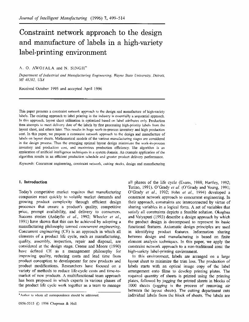
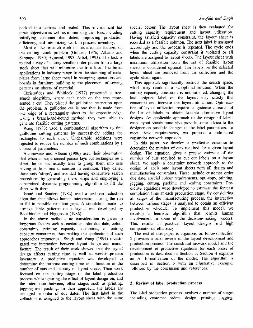
The design of label sheets starts with retrieval of customers' orders from inventory. The inventory of orders contains many variations of printing requirements and processing requirements. Layouts are divided into two basic categories: combination (combo)jobs (Fig. 1) and straight jobs (Fig. 2). Combo jobs consist of a combination of different customer orders printed on the same sheet, while straight runs have only one customer's order on a sheet. Straight orders require special consideration: hence enough labels are usually ordered to produce an adequately long run to achieve a good price. Combo jobs are more standard in nature, and result in five standard colours with dark blue, brown or black as the sixth colour.
C C C C C C D C C D C C D
A
B
A
B
Fig. 1. Layout of a combination job.
E E
E E
E
Fig. 2. Layout of a straight job.
501
To design a layout, rush orders are taken aside for consideration. Using colour, quantity of labels required and run length of sheets as constraints, rush labels that could be printed together are selected. Existing presses have six-colour printing units, and the various jobs have only four or five colours in common: hence jobs must be split into separate runs. The sixth colour of a label is usually referred to as the special colour. Once the rush orders are satisfied, orders from inventory can be taken to fill the remaining portion of the sheet, provided the constraints for colour and quantity are met. Other parameters considered when filling the sheet are paper utilization, label positioning, and maximization of run lengths.
When the layout is completed, a computer check is done to ensure that the correct tolerances and fit are achieved. The opti-copy machine copies all the individual film negatives of the labels desired on that layout sheet to one large film sheet. Six such sheets are produced, one for each colour needed in the final label, and then used to burn printing plates. Plates are stored until needed by the press operators.
2.2. Production stage
The production starts in the pressroom. The printing plates are used to print the required number of sheets. Printed material is weighed into blocks of 1000 sheets, and cardboard is inserted on the bottom of the block. The blocks are then jogged to square up all comers, and the air is removed from between the sheets. The blocks are then slid on the air board and stacked, with the air board between blocks, on skids, ready for cutting.
Cutter programming takes place based on the layout and information contained within the sales docket regarding the label dimensions. The blocks of 1000 sheets are slid off the air board and onto the cutter table, where they are cut. The cut labels are then passed down the table to the next person, who inserts the bundle into the string-tying machine. The machine binds the bundle together and sends it through the shrink-wrap machine and down to the packing line.
The cut labels travel down a conveyor to the boxing station, where pre-made boxes are waiting. The labels are sorted into paper boxes and then sealed using the sealing maching. The warehouse handles both raw materials and finished products. The warehouse also stores any overflow material from the rest of the plant, and approximately 10-20% of floor area is used to store the overflow material. The layout design and manufacturing process explained above results in high WIP inventory and late delivery to customers (Singh and Wang, 1994). In the next section, we describe a constraint network model for optimal design of labels onto layout, and efficient production.
502
3. The model
The following assumptions were made in the model and alogrithm:
(1) Transportation time between production stages is negligible;
(2) Satisfying all production capacity constraints corresponds to meeting the due date requirement;
(3) Each stage of the manufacturing process handles one layout sheet at any give time.
3.1. Opti-copy
The opti-copy machine first checks the layout sheet for tolerance and accuracy, then copies film negatives of labels onto a large film sheet. Six such sheets are produced, one for each colour needed in the final label. The computer checking and opti-copy time is a function of the number of labels, N, to copy. The film sheets are used to burn printing plates, which are stored in a buffer until required by the printing department. The time to produce printing plates is also a function of the number of labels on the layout. The forecast production time at the opti-copy department is defined as
OC= HI +¢ZlN
where OC = total opti-copy and plating time; H1 = machine set-up time; N = number of labels on the layout; al --constant, estimated from real-life data.
3.2. Printing
At the printing department the plates and stock of plain sheets are input to the printing machine. The printing time is a function of the quantity of sheets, QS, to print. The printed sheets are stored as WIP inventory until required by the jogging department. The forecast production time at this department is modelled as
PT = H2 + a2 QS
where PT=to ta l printing time; H2 =machine set-up time; QS = quantity of sheets to produce; a2 = constant, estimated from real-life data.
3.3 Jogging
At this stage, the sheets are jogged in blocks of 1000 sheets. The jogging process involves evacuating air between the sheets. The jogging machine handles one block at a time. The jogging time is a function of the number of layout blocks, and is defined as
JT = H3 + a3NB
where JT = total jogging time; H 3 = machine set-up time;
Awofala and Singh
NB ---- number of layout blocks = QS/IO00; a2 = constant, estimated from real-life data.
3.4. Cutting
The cutting time was determined from previous work (Singh and Wang, 1994) as
CT = A 1 QS Az N C A3
where CT = total cutting time; NC = number of cuts; A1, A2, A3 are constants and exponents estimated from real- life data.
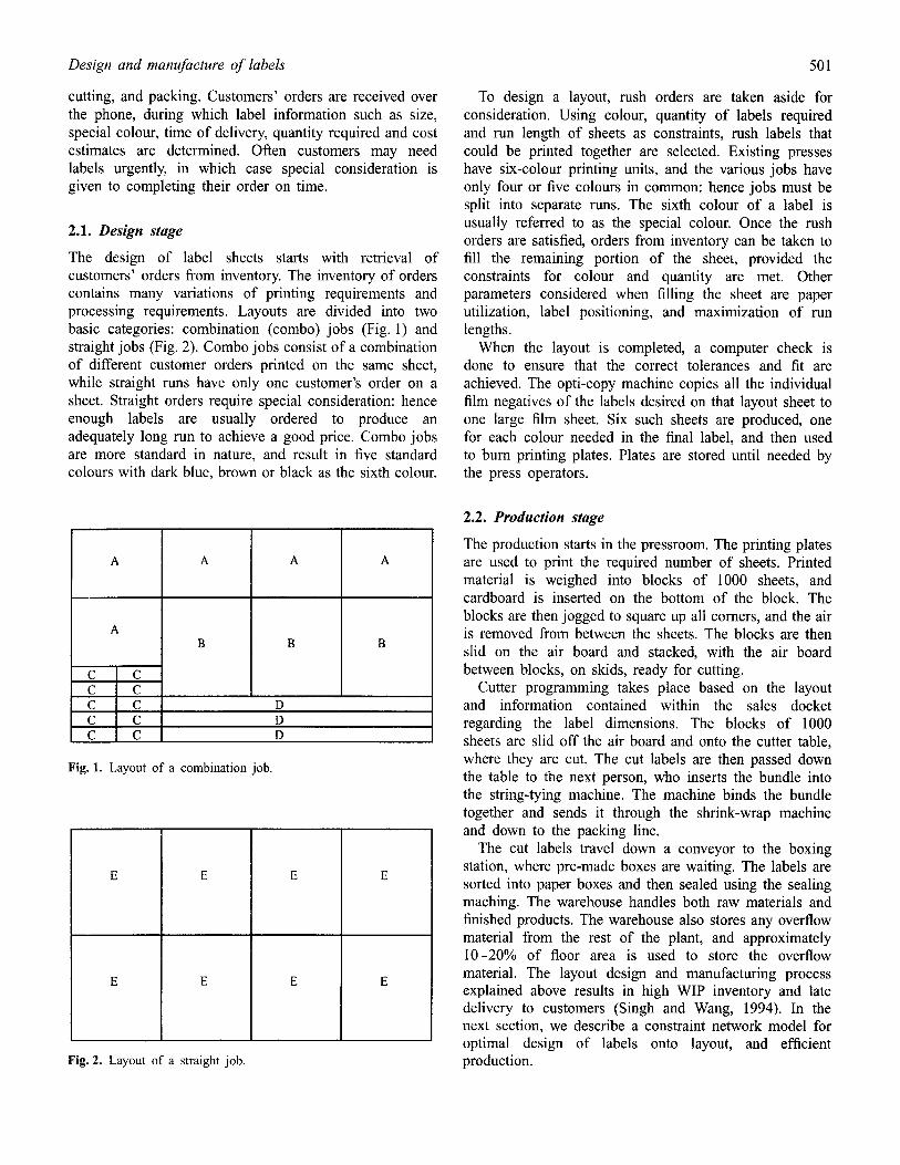
In this research, a predictive equation is developed to determine the number of cuts, NC, required for a layout. Consider the layout in Fig. 3, which has six labels. First, the layout has to be trimmed on all four sides (four cuts) to obtain the correct tolerance and fit on label edges. Then a cut along boundary line 1 separates the layout into two parts. Two cuts (2 and 3) are needed to obtain labels A, B and C. Cutting along lines 4 and 5 on the second part produces labels D, E and E Thus, a total of 9 cuts (5 + 4) are required for this layout.
The proposed equation is:
NC = ( n - 1 ) + 4
where n = number of labels on the layout sheet.
3.5. Packing and sealing
In this department, bundles of labels are manually packed into boxes and sealed by a sealing machine. The packing and sealing time is modelled as
N
PS = Z ( a 4 / + asi)(AiNB)/BXi i=1
where PS = total packing and sealing time of all labels on a layout sheet; BXi = number of label blocks of type i per box; Ai = number of label type i on the layout sheet; o~4i = time to pack label type i in a box (determined from standard timetable); asi = time to seal one box of label type i (estimated from real-life data).
A
D
(21
(41
B
E
(3' C
F (51
(1)
Fig. 3. Detailed layout of labels.
Design and manufacture of labels
3 . 6 . Total production time
The total production time of layout sheet j is not the sum of all production times at the various stages described ab ov e:
Tj 7 ~ OCj + PTj + JTj + CTj + PSj
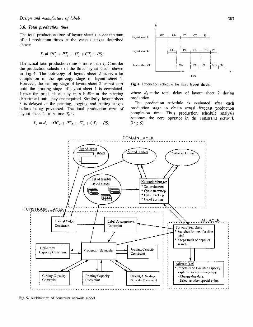
The actual total production time is more than Tj. Consider the production schedule of the three layout sheets shown in Fig. 4. The opti-copy of layout sheet 2 starts after completion of the opti-copy stage of layout sheet 1. However, the printing stage of layout sheet 2 cannot start until the printing stage of layout sheet 1 is completed. Hence the print plates stay in a buffer at the printing department until they are required. Similarly, layout sheet 3 is delayed at the printing, jogging and cutting stages before being processed. The total production time of layout sheet 2 from time To is
T2 = d2 + 0C2 + PT2 + JT2 + CT2 + PS2
503
To
Layout sheet #1
Layout sheet #2
Layout sheet #3
O G PTI JT~ CT~ PS~ I I
OC: P% JT2 CT: PS~
O G I PT, I JT3 I CT'~ [PS , [
Time
Fig. 4. Production schedule for three layout sheets.
where de = the total delay of layout sheet 2 during production.
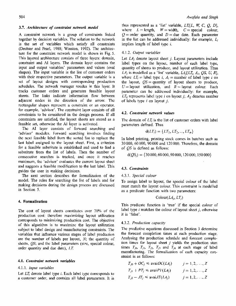
The production schedule is evaluated after each production stage to obtain actual forecast production completion time. Thus production schedule analysis becomes the core operator in the constraint network (Fig. 5).
DOMAIN LAYER . . . . . . . . . . . . . . . . . . . . . . . . . . . . . . . . . . . . . . . . . . . . . . . . . . . . . . . . . . . . . . . . . . . . . . . . . . . . . . . . •
Orders
CONSTRAINT LAYER
of feasible layout sheets Network Manager
[
~ ~ _ _ . _ ~ * Set evaluation • Cycle start/stop • Cycle tracking • Label Sorting
/ Label Arrangement Constraint ] / " Cons2raint
Opti-Copy ~ ~ Jogging Capacity Capacity Constraint Production Scheduler Constraint
lcuttn Capacty I Print n Capacty I [Pack ng Seaing Constraint Constraint Capacity Constraint
ER.. Forward Searching * Searches for next feasible
label * Keeps track of depth of
search.
Advisor (e.g) * If there is no available capacity.
- split order into two orders. - Change due date. - Select another special color.
4 . . . . . . . . . . . . . . . . . . . . . . . . . . . . . . . . . . . .
Fig. 5. Architecture of constraint network model.
504
3.7. Architecture of constraint network model
A constraint network is a group of constraints linked together by decision variables. The solution to the network is the set of variables which satisfy all constraints (Dechter and Pearl, 1988; Winston, 1992). The architec- ture for the constraint network model is shown in Fig. 5. This layered architecture consists of three layers: domain, constraint and AI layers. The domain layer contains the input and output variables' parameters and values (oval shapes). The input variable is the list of customer orders with their respective parameters. The output variable is a set of layout designs with corresponding production schedules. The network manager resides in this layer. It tracks customer orders and generates feasible layout sheets. The links indicate information flow between adjacent nodes in the direction of the arrow. The rectangular shapes represent a constraint or an operator, for example, 'advisor'. The constraint layer consists of all constraints to be considered in the design process. If all constraints are satisfied, the layout sheets are stored as a feasible set, otherwise the AI layer is activated.
The AI layer consists of forward searching and 'advisor' modules. Forward searching involves finding the next feasible label from the sorted list to replace the last label assigned to the layout sheet. First, a criterion for a feasible substitute is established and used to find a substitute from the list of labels. Then the number of consecutive searches is tracked, and once it reaches maximum, the 'advisor' evaluates the current layout sheet and suggests a feasible modification to the last label. This guides the user in making decisions.
The next section describes the formalization of the model. The rules for searching the list of labels and for making decisions during the design process are discussed in Section 5.
4. Formalization
The cost of layout sheets constitutes over 70% of the production cost: therefore maximizing layout utilization corresponds to minimizing production cost. The objective of this algorithm is to maximize the layout utilization subject to label design and manufacturing constraints. The variables that influence various stages of label production are the number of labels per layout, N; the quantity of sheets, QS; and the label parameters (size, special colour, order quantity and due date), LT.
4.1. Constraint network variables
4.1.1. Input variables Let LT/denote label type i. Each label type corresponds to a customer order, and contains all label parameters. It is
Awofala and Singh
thus represented as a 'list' variable, LTi[L, W, C, Q, D], where L = length, W = width, C = special colour, Q = order quantity, and D = due date. Each parameter in the list can be addressed individually: for example, Li implies length of label type i.
4.1.2. Output variables Let LAj denote layout sheet j. Layout parameters include label types on the layout, number of each label type, quantity of sheets to produce, and layout utilization. Thus LAj is modelled as a 'list' variable, LAj[LTi, Ai, QS, U, R], where LT/= label type i, Ai = number of label type i on the layout, QS = quantity of layout sheets to produce, U--layout utilization, and R=layout colour. Each parameter can be addressed individually: for example, LTij represents label type i on layout j; A/j denotes number of labels type i on layout j.
4.2. Constraint network values
The domain of LT/is the list of customer orders with label parameters defined. Thus
d(LTi) = {LT1, LT2, ..., LTm}
In label printing, printing stock comes in batches such as 30 000, 60 000, 90 000 and 120 000. Therefore, the domain of QS is defined as follows:
d(QSj) = {30 000, 60 000, 90 000, 120 000, 150 000}
4.3. Constraints
4.3.1. Special colour To assign label to layout, the special colour of the label must match the layout colour. This constraint is modelled as a predicate function with two parameters:
Colour( LAj, LTj)
This predicate function is 'true' if the special colour of label type i matches the colour of layout sheet j, otherwise it is 'false'.
4.3.2. Production capacity The predictive equations discussed in Section 3 determine the forecast completion times at each production stage. Analysing the production schedule and forecast comple- tion times for layout sheet j yields the production start times TjO , Tjl , Tj2 , Tj3 and Tj4 at each stage of label manufacturing. The formalization of each capacity con- straint is as follows:
Tjo + OCj ~ avaiOC(LAj)
Tjl + PT/ ~ avaiPT(LAj)
Tj2 + JTj ~ avaiJT(LAj)
j---- 1 , 2 , . . . , Z
j - - 1 , 2 , . . . , Z
j - - 1 , 2 , . . . , Z

Design and manufacture o f labels 505
Tj3 .-t.- CTj ~- avaiCT(LAj) j = 1 ,2 , . . . , Z
Tj4 + PSi <~ avaiPS(LAj) j = 1 ,2 , . . . , Z
where OCj, PTj, JTj, C~, PSi represent the forecast opti- copy, printing, jogging, cutting and packing completion times of layout sheet j respectively; avaiOC (LAj) is a predicate function that returns the available opti-copy capacity (from time To) within the minimum due date of labels on layout sheet LAj; similar functions (avaiPT, avaiJT, avaiCT, avaiPS) apply to the printing, jogging, cutting and packing stages of the production cycle respectively.
4.3.3. Label arrangement on layout
The layout sheet utilization is determined after the labels have been arranged on the layout. The arrangement of the labels on the layout sheet is an important factor in minimizing trim loss. Dietrich and Yakowitz (1991) developed a rule-based approach to the trim-loss problem. In their algorithm, a set of rules is used to place labels on the layout sheet from one edge to the opposite edge to minimize the trim loss. We adopt this approach in this paper to determine the optimal label arrangement. It is modelled as a function that returns the layout sheet utilization, or zero if the label arrangement exceeds the layout sheet area:
Arrang(L Tj, LCj)
The output of this function is the LTj parameters and location coordinates of each label on the layout sheet, where LCj is a list variable of the location coordinates of labels on layout sheet j. For example,
LCj[1, (0, O, L), (0, 12, L), 2, (0, 24, W)]
me an s:
label type 1: label 1 locates at (0, 0) with its length parallel to the layout sheet length; label 1 locates at (0, 12) with its length parallel to the layout sheet length;
label type 2: label 2 locates at (0, 24) with its length parallel to the layout sheet length.
The next section describes the algorithm with an illustrative example. The criteria for searching the list of labels and rules for selecting the optimal layout plan are discussed.
5.1. The algorithm
Step 0
Given m customer orders, LT1, LTz, . . . LTm (LTi C ~V) with their parameters, i.e. due date, special colour, quantity and size, arrange the m orders in an ascending sequence according to their due dates:
D1 <~ D2 <~ Dj .... ~ DM
Step 1
Define a set of k printing sheets LS, where each sheet LAs in the set corresponds to a special colour in the k colour group:
LS[ LA 1, LA2, ..., LAk].
Step 2
Define AD = 0, V = 0. Assign ~p --- ~p'. If ~p' = q~, go to step 9, ELSE go to step 3; where AD = program control variable, V = counter variable.
Step 3
Select the first label LTj in 9 ' . IF the label is marked 'previously assigned and replaced', THEN select the next label. ELSE continue. Find layout sheet LAj that satisfies the colour constraint
Colour(LAj, LT/)
IF the layout sheet is an optimal sheet (i.e. utilization ~>99%), THEN select the next label.
Step 4
Arrange the labels assigned to the layout sheet using the rule-based approach (Dietrich and Yakowitz, 1991) and the domain of printing sheets d(QSj).
Step 5
Calculate the forecast completion times for all the sheets in LS at each stage of production. Estimate the production schedule for the set of layout sheets. For each layout sheet in the set, determine if all production capacity constraints are satisfied. IF steps 4 and 5 are 'true' go to step 8, ELSE go to step 6.
5. The algorithm
In this section, we describe the heuristic alogrithm developed for implementing the constraint network model. First we describe the alogrithm, then we describe an illustrative example to explain the algorithm.
Step 6
IF AD = 1, go to step 9. If V = max., go to step 7, ELSE Determine the search criterion. Set V = V + 1. Search through ~p' to find the next feasible label Lf. Replace the previous label with Lf. (The number of labels in ~p' remains the same.) Mark the prior label 'previously assigned and replaced'. Go to step 4.
506
Step 7
Evaluate the current layout set and make suggestions on possible modifications to the label. Set AD = 1. IF the domain user makes any changes to the label go to step 4. ELSE go to step 9.
Step 8
Set AD = 0. Store this label-on-layout set LS as a feasible layout plan. Go to step 3.
Step 9
Select the layout plan with the highest paper utilization from all the feasible plans generated.
Step 10
Stop.
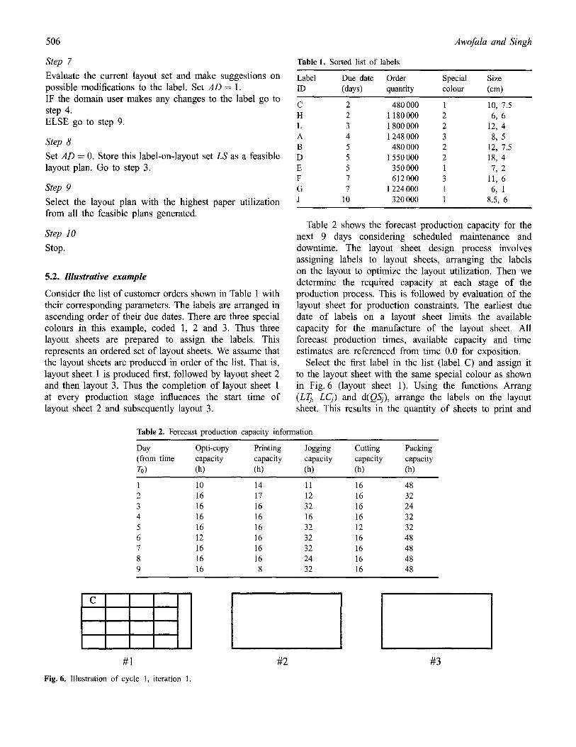
5.2. Illustrative example
Consider the list of customer orders shown in Table 1 with their corresponding parameters. The labels are arranged in ascending order of their due dates. There are three special colours in this example, coded 1, 2 and 3. Thus three layout sheets are prepared to assign the labels. This represents an ordered set of layout sheets. We assume that the layout sheets are produced in order of the list. That is, layout sheet 1 is produced first, followed by layout sheet 2 and then layout 3. Thus the completion of layout sheet 1 at every production stage influences the start time of layout sheet 2 and subsequently layout 3.
Awofala and Singh
Table 1. Sorted list of labels
Label Due date Order Special Size ID (days) quantity colour (cm)
C 2 480000 1 10, 7.5 H 2 1 180 000 2 6, 6 L 3 1 800 000 2 12, 4 A 4 1 248000 3 8, 5 B 5 480000 2 12, 7.5 D 5 1550000 2 18, 4 E 5 350000 1 7, 2 F 7 612 000 3 11, 6 G 7 1 224 000 1 6, 1 J 10 320 000 1 8.5, 6
Table 2 shows the forecast production capacity for the next 9 days considering scheduled maintenance and downtime. The layout sheet design process involves assigning labels to layout sheets, arranging the labels on the layout to optimize the layout utilization. Then we determine the required capacity at each stage of the production process. This is followed by evaluation of the layout sheet for production constraints. The earliest due date of labels on a layout sheet limits the available capacity for the manufacture of the layout sheet. All forecast production times, available capacity and time estimates are referenced from time 0.0 for exposition.
Select the first label in the list (label C) and assign it to the layout sheet with the same special colour as shown in Fig. 6 (layout sheet 1). Using the functions Arrang (LTj, LCj) and d(QSfl, arrange the labels on the layout sheet. This results in the quantity of sheets to print and
Table 2. Forecast production capacity information
Day Opti-copy Printing Jogging Cutting Packing (from t ime capacity capacity capac i ty capac i ty capacity To) (h) (h) (h) (h) (h)
1 10 14 11 16 48 2 16 17 12 16 32 3 16 16 32 16 24 4 16 16 16 16 32 5 16 16 32 12 32 6 12 16 32 16 48 7 16 16 32 16 48 8 16 16 24 16 48 9 16 8 32 16 48
C
#1
Fig. 6. Illustration of cycle 1, iteration 1.
#2 #3
Design and manufacture of labels
the number of each label on the layout. As mentioned earlier, the layout sheets come in batches, with a minimum of 30 000 sheets and an increment of 30 000 sheets. To obtain 480 000 labels, the number of labels per layout sheet, A1, is 480000/30000, which equals 16. If 16 labels can be arranged optimally on the layout sheet, then the layout sheet is accepted. Otherwise, the number of sheets increases to 60 000. From this arrangement, the layout sheet utilization is 88%. The number of label type C per layout sheet, A1, is 16.
The next step is to determine whether layout sheet 1 satisfies all production constraints. Using the layout parameters, the forecast completion time at each stage of production is determined, i.e. 0C1, PT1, JTI, CT1 and KT~. To determine the forecast start time for layout sheet 1, we evaluate the production schedule for the current layout in production or the prior layout sheet. The forecast completion time of the prior label sheet indicates the start of the next layout sheet at each production stage, i.e. 7'1o, Tll, TI2, 7"13, T14. If no previous layout sheet exists or is scheduled (e.g. at the start of a new production shift) then
Tll = To + OC1
TI2 = Tll + PT1
T13 ~- T12 + JT1
T14 -- T13 + CTI
The forecast completion time is compared with the available production time at each production stage. Label C is due in 2 days. From Table 2 there are 21 h of printing time available in the next 2 days: therefore layout sheet 1 can be printed if
T11 + PTa <~ 21
There are only 23 h for sheet jogging within the next 2 days. This layout sheet satisfies the jogging capacity constraint if
T12 + JT1 <~ 23
The same analogy is used at the other production stages, as described in Fig. 6. Because packing and sealing is the last manufacturing process, it is assumed that satisfying the packing and sealing constraints corresponds to meeting the due date. Layout sheet 1 is
507
the first sheet at the start of production. Therefore the start of printing, Tll, succeeds the completion of opti- copy operation. Jogging operation start time T12 occurs after the completion of printing operation, and so on. Because layout sheet 1 satisfies all production constraints, the layout set is stored as a feasible layout plan.
Iteration 1
QS = 30 000
A1 = 16
U = 88%
To = 0, OCl = 3.5 h, PTl = 5.0 h, JTl = 4.5 h, CT1
= 5.8 h, PS1 = 6.5 h
T10 = 0, Tll = 3.5, T12 = 8.5, T13 = 13, T14 = 18.8
T~o + OCI ~ 0 + 3.5 = 3.5 < 2 6
(opti-copy capacity for next 2 days)
Tll + PT1 =~ 3 . 5 + 5 . 0 = 8 .5<21
(printing capacity for next 2 days)
TI2 + JT1 =~ 8.5 + 4.5 = 13.0 < 64
(jogging capacity for next 2 days)
T13 + CT1 =:k 13 + 5.8 = 18.8 < 32
(cutting capacity for next 2 days)
T14 + PS1 =~ 18.8 + 6.5 = 25.3 < 80
(packing capacity for next 2 days)
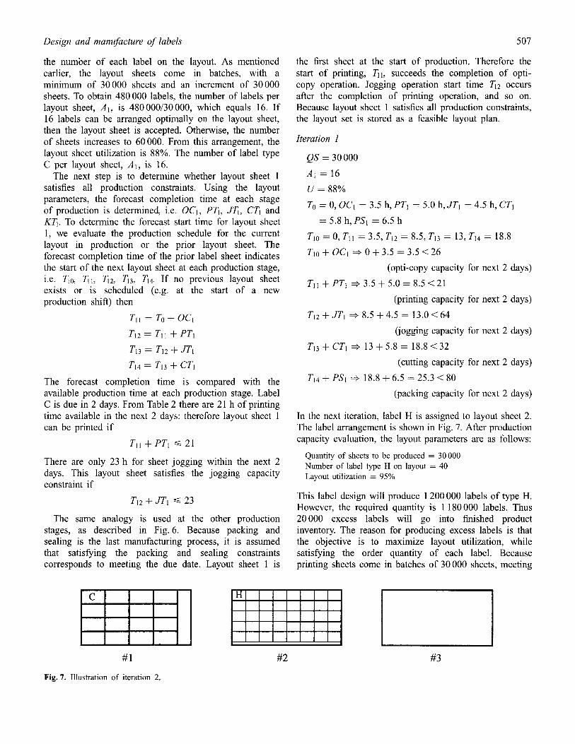
In the next iteration, label H is assigned to layout sheet 2. The label arrangement is shown in Fig. 7. After production capacity evaluation, the layout parameters are as follows:
Quantity of sheets to be produced = 30 000 Number of label type H on layout = 40 Layout utilization = 95%
This label design will produce 1 200 000 labels of type H. However, the required quantity is 1 180 000 labels. Thus 20000 excess labels will go into finished product inventory. The reason for producing excess labels is that the objective is to maximize layout utilization, while satisfying the order quantity of each label. Because printing sheets come in batches of 30 000 sheets, meeting
C H
#1 #2 #3
Fig. 7. Illustration of iteration 2.

508
the order quantity of one label on the layout may result in excess labels for another label on the layout. As mentioned earlier, 9 out of 10 orders are repeat orders. Demand for the excess labels will occur within a short time.
Layout sheet 2 follows label sheet 1 in the production schedule. The opti-copy operation for sheet 2 starts after completing opti-copy operation for sheet 1. Printing of layout sheet 2 starts after the completion of opti-copy operation for sheet 2 or printing operation of sheet 1, whichever is later. Column 4 of Table 3 shows the starting time to manufacture layout sheet 2. The forecast capacity for layout sheet 2 is determined by using model formulations. The completion time results from the addition of forecast capacity to the start time at each stage. Compared with the available production capacities, layout sheet 2 satisfies all production constraints. This layout set is stored as a feasible layout plan (Fig. 7, Table 3).
Iteration 2
QS = 30 000 QS = 30 000
AI = 16 A2 = 40
U = 88% U = 95%
0C2 = 4.5 h, PT2 = 5.0 h, JT2 ---- 4.5 h, CT2 = 6.5 h,
PS2 ---- 6.0 h
Iteration 3
QS = 30 000
AI = 16
U = 88%
O C 2 = 7.0 h, PT2 = 9.0 h,
Awofala and Singh
QS = 90 000
A2 = 16, A3 =- 20,
U = 99%
JT2 = 6.5, CT2 = 7.8 h,
PSa = 7.0 h
In the third iteration, label L is assigned to layout sheet 2. After arranging the labels on the layout sheet, the obtained layout parameters are as shown in Fig. 8. However, the layout sheet cannot satisfy jogging capacity constraint. The required quantity of sheets has increased to 90 000, which results in a forecast jogging completion time greater than the available jogging capacity. Table 4 shows the production capacity requirements for layout sheet 2, which consists of labels B and L. Intuitively, a label with a smaller order quantity will probably satisfy the jogging capacity constraint. Thus, the criterion for searching through the list of labels for a feasible substitute is 'same special colour but smaller order quantity'.
Mathematically, we defined this criterion for a feasible substitute label LT~ as
LTf[C] = LT1[C] and LTf[Q] < LT1 [Q]
where LT1[C] denotes the special colour of label type L, and LT1[Q] denotes the order quantity of label type L.
Table 3. Production capacity requirement for layout sheet 2, label H
Completion Forecast Production time of capacity for stage layout 1 layout 2
Start Available time of Completion capacity layout 2, time of for next ~/2j layout 2 2 days
Opti-copy, OC 3.5 4.5 3.5 8.0 26.0 Printing, PT 8.5 5.0 8.5 13.5 31.0 Jogging, JT 13.0 4.5 13.5 18.0 23.0 Cutting, CT 18.8 6.5 18.8 25.3 32.0 Packing, PS 25.3 6.0 25.3 31.3 80.0
Table 4. Production capacity requirement for layout sheet 2, labels H and L
Start Completion Forecast time of
Production time of capacity for layout 2, stage layout 1 layout 2 T2j
Completion time of layout 2
Available capacity for next 2 days
Opti-copy, OC 3.5 7.0 3.5 10.5 26.0 Printing, PT 8.5 9.0 8.5 17.5 31.0 Jogging, JT 13.0 6.5 17.5 24.0 23.0 Cutting, CT 18.8 7.8 19.5 27.3 32.0 Packing, PS 25.3 7.0 26.6 33.6 80.0
Note that jogging capacity is violated, i.e. 24.0 > 23.0 (the available capacity).

Design and manufacture of labels
C HI ] I I I I I I
509
#1
Fig. 8. Illustration of iteration 3.
e,¢
L #2 #3
Label B meets this requirement. It has the same speical colour and a smaller order quantity, and hence replaces label L on layout sheet 2. After executing the label arrangement function, the required quantity of sheets reduces to 60 000. The forecast jogging completion time is now 20 h from time To. This satisfies the jogging capacity constraint, i.e. T22 q-JT2 ~ 23. Having satisfied all other constraints, this layout set (Fig. 9) is stored as a feasible layout plan.
Iteration 4
QS = 30 000
Al = 16
U = 88%
0 C 2 = 6.0 h, P T 2 = 7.0 h,
QS= 60000
A2 = 24, A4 = 8
U = 99%
JT2 = 5.5 h, CT2 = 6.5 h,
PS2 = 6.0 h
Tz0 = 3.5, T21 = 9.5, T22 = 15.5, Tz3 = 18.8,/124 = 25.3
7"22 + JT2 ~ 15.5 + 5.5 = 21.0 < 23
(jogging capacity for next 2 days)
C H
Jogging capacity constraint is satisfied, as well as the other production capacity constraints.
The list of remaining labels is [L', A, D, E, F, G, J]. The first label in the list is label L. We cannot assign this label because it has been marked, which means that it has been assigned and replaced in the current layout set. Layout sheet 2 has attained maximum utilization (i.e. U ~ > 99%). Therefore this layout sheet is optimal. The following rule provides a guideline for making the next label assignment:
(1) Assign the next label only if it does not have the same special colour as layout sheet 2.
(2) Process the label on the layout sheet. Accept the layout design if all subsequent layout sheets in the set can be completed within their available production capacity.
Using the above rules, the next label assignment in this example is label A. The special colour for the label matches that of layout sheet 3. Thus we assign label A to layout sheet 3. Figure 10 shows the layout sheet design. Constraint network analysis indicates that layout sheet 3 can be produced within the available production capacity. Hence the layout set becomes a feasible layout plan.
B
#1
Fig. 9. Illustration of iteration 4.
#2 #3
C H A
B
#1 #2 #3
Fig. 10. Illustration of iteration 5.
510 Awofala and Singh
C Iil III HI III
H
B
A
#1 #2 #3
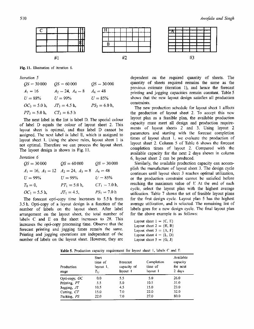
Fig. 11. Illustration of iteration 6.
Iteration 5 QS = 30 000 OS = 60 000
A1 = 16 A2 = 24, A4 = 8
U = 88% U = 99%
0C3 = 5.0 h, JT3 = 4.5 h,
PT3 = 5.0 h, CT3 = 6.5 h
QS = 30 000
A6 = 48
U = 85%
PS3 = 6.0 h,
The next label in the list is label D. The special colour of label D equals the colour of layout sheet 2. This layout sheet is optimal, and thus label D cannot be assigned. The next label is label E, which is assigned to layout sheet 1. Using the above rules, layout sheet 1 is not optimal. Therefore we can process the layout sheet. The layout design is shown in Fig. 11.
Iteration 6 QS = 30 000 QS --- 60 000 QS = 30 000
AI ---- 16, A5 = 12 A2 = 24, A3 = 8 A6 = 48
U = 99% U = 99% U -- 85%
To = O, PT1 = 5.0 h, CT1 = 7.0 h,
0C1 = 5.5 h, JT1 = 4.5, PS1 = 7.0 h
The forecast opti-copy time increases to 5.5 h from 3.5 h. Opti-copy of a layout design is a function of the number of labels on the layout sheet. After label arrangement on the layout sheet, the total number of labels C and E on the sheet increases to 28. This increases the opti-copy processing time. Observe that the forecast printing and jogging times remain the same. Printing and jogging operations are independent of the number of labels on the layout sheet. However, they are
dependent on the required quantity of sheets. The quantity of sheets required remains the same as the previous estimate (iteration 1), and hence the forecast printing and jogging capacities remain constant. Table 5 shows that the new layout design satisfies all production constraints.
The new production schedule for layout sheet 1 affects the production of layout sheet 2. To accept this new layout plan as a feasible plan, the available production capacity must meet all design and production require- ments of layout sheets 2 and 3. Using layout 2 parameters and starting with the forecast completion times of layout sheet 1, we evaluate the production of layout sheet 2. Column 5 of Table 6 shows the forecast completion times of layout 2. Compared with the available capacity for the next 2 days shown in column 6, layout sheet 2 can be produced.
Similarly, the available production capacity can accom- plish the manufacture of layout sheet 3. The design cycle continues until layout sheet 3 reaches optimal utilization, or the production constraint cannot be satisfied before reaching the maximum value of V. At the end of each cycle, select the layout plan with the highest average utilization. Table 7 shows the set of feasible layout plans for the first design cycle. Layout plan 5 has the highest average utilization, and is selected. The remaining list of labels goes for a new design cycle. The final layout plan for the above example is as follows:
Layout sheet 1 = {C, E} Layout sheet 2 = {H, B} Layout sheet 3 = {A, F} Layout sheet 4 = {L, D} Layout sheet 5 = {G, J}
Table 5. Production capacity requirement for layout sheet 1, labels C and E
Opti-copy, OC 0.0 5.5 5.0 26.0 Printing, PT 5.5 5.0 10.5 31.0 Jogging, JT 10.5 4.5 15.0 23.0 Cutting, CT 15.0 7.0 22.0 32.0 Packing, PS 22.0 7.0 27.0 80.0
Start Available time of Forecast Completion capacity
Production layout 1, capacity of time of for next stage T U layout 1 layout 1 2 days
Design and manufacture of labels
Table 6. Revised production capacity requirement for layout sheet 2, labels H and B
511
Start Completion Forecast time of
Production time of capacity for layout 2, stage layout 1 layout 2 T2j
Available Completion capacity time of for next layout 2 2 days
Opti-copy, OC 5.0 6.0 5.0 11.0 26.0 Printing, PT 10.5 7.0 11.0 18.0 31.0 Jogging, JT 15.0 5.5 17.5 23.0 23.0 Cutting, CT 22.0 6.5 22.0 23.0 32.0 Packing, PS 27.0 6.0 28.5 34.5 80.0
Table 7. Parameters of feasible layout plans
Layout Average Layout Layout utilization utilization plan set (%) (%)
1 Sheet 1: {C} 88.0 88.0
2 Sheet 1: {C} 88.0 91.5 Sheet 2: {H} 95.0
3 Sheet 1: {C} 88.0 93.5 Sheet 2: {H, B} 99.0
4 Sheet 1: {C} 88.0 92.3 Sheet 2: {H, B} 99.0 Sheet 3: {A} 90.0
5 Sheet 1: {C, E} 99.0 96.0 Sheet 2: {H, B} 99.0 Sheet 3: {A} 90.0
6 Sheet 1: {C, E} 99.0 98.0 Sheet 2: {H, B} 99.0 Sheet 3: {A, F} 96.0
5.3. Heuristic definitions
Search criterion
When a label is assigned to a layout sheet, first we find the optimal arrangement of labels on the layout sheet. Then the order quantity and number of labels on the layout determine the quantity of layout sheets. The design objective is to maximize layout utilization and attain the maximum order quantity for each label on the layout. As mentioned earlier, any excess labels produced will be demanded in subsequent orders. The forecast completion times at various stages of production are functions of layout sheet quantity (QS). Hence increasing the produc- tion quantity of layout sheets may result in a violation of the production constraints. This implies that the quantity of layout sheets should be reduced. The quantity of layout sheets is a function of label size and order quantity. A
substitute label with a smaller order quantity and/or label size may result in a smaller quantity of layout sheets for production. The following describes the rules for selecting feasible substitutes.
It is worth noting that a substitute label must result in greater layout sheet utilization. Otherwise, the constraint network is considered not satisfied for that iteration.
Order quantity:
(1) Select a label with smaller label area and smaller order quantity than the current label;
(2) Select a label with smaller label area and approximately equal order quantity as the current label;
(3) Select a label with smaller label area and larger order quantity than the current label.
Label area:
(1) Select a label with smaller order quantity and approximately equal label area as the current label;
(2) Select a label with smaller order quantity and larger label area than the current label.
The most effective set of rules can be determined through experiments with a variety of layout sheet sizes and order pieces.
Selecting the optimal layout sheets
The layout development cycle ends when one of the following occurs:
(1) Every label has been assigned to a layout sheet; (2) The constraint network is not satisfied after
acknowledging suggestions from the advisor module; (3) All layout sheets have attained maximum utiliza-
tion.
Each cycle generates a number of feasible layout plans. The question arises as to how to select the optimal layout plan from a list of possible candidates. As mentioned earlier, a layout sheet may result in excess labels. Thus there is the question of how to minimize the excess finished product inventory. Intuitively, the layout set with
512
the minimum excess labels should be selected. However, this may result in suboptimal layout sheet utilization. The following rules describe the strategy for selecting optimal layout design from possible candidates:
Priority 1: Select the layout plan with the maximum average utilization;
Priority 2: Select the layout plan with the minimum average excess labels;
Priority 3: Select the layout plan containing the maximum number of label types;
Priority 4: Select the layout plan with the minimum average quantity of layout sheets.
Layout sheets are selected from the list of feasible sets using priority 1 as criterion. If there is more than one unique set of layout sheets, priority 2 is applied to the candidate sets. Next, select layout sets using priority 3 and 4 respectively until a unique solution is obtained.
The advisor module
The advisor module enables the designer to be involved in some of the decision-making process. In some situations, changing the order quantity or due date may improve the layout sheet utilization and/or reduce the excess finished labels. The label parameters are defined when a customer places a order. Therefore changes cannot be made to the label parameters without consulting with the customer. Moreover, frequent changes to label parameters may be detrimental to customer satisfaction. Thus the domain expert makes the decision whether to effect any changes. During the design cycle, the constraint network attempts to replace inapplicable labels by searching the list for a feasible substitute. Upon reaching the maximum number of searches, the advisor evaluates the layout sheets and label, and makes suggestions on feasible changes to the last label assigned. The following describes the guidelines used by the advisor in making suggestions:
(1) Reduce the order quantity of the label by splitting the order into two separate orders (same size and special colour but different due dates and order quantities);
(2) Extend the due date of the label; (3) Change the special colour of the label.
5.4. Decision tree
A cycle starts with a list of labels to be designed on layout sheets. A layout set is prepared depending on the number of special colours. A given cycle uses one set of layout sheets. An iteration starts with a label assigned to a layout sheet in the set with the same special colour in the set. The layout set is propagated through the constraint network. After satisfying all constraints in the network, the layout set is recorded as a feasible layout set. Then the next label is assigned to the corresponding layout sheet in
Awofala and Singh
the set and the constraint network evaluation process is repeated. Every iteration results in one of three possible outcomes, as follows:
(1) No more labels in the list; (2) All layout sheets are optimal; (3) All constraints are satisfied; (4) One or more constraints is violated.
If the list is empty, or all layout sheets are optimal, the cycle ends. If all constraints are satisfied, the layout set is stored as a feasible layout plan. The next label is assigned, and the next iteration starts: i.e. the cycle continues. However, if after an iteration one or more constraints is violated - termed a constraint fault - the AI module is activated to search for a feasible substitute. After a maximum of V consecutive searches, the advisor is invoked. Suggestions are generated on possible modifications to the current label. If any change is made, the iteration is repeated; otherwise the cycle ends. At the end of every cycle, the optimal layout is selected using the rules stated earlier, and the list of labels is updated. The decision subtree is shown in Fig. 12.
O
/ ~ ~ I T E R A T I O N
END NEXT LABEL CONSTRAINT FAULT 9
INCt FORWARD SEARCHING SEAl COU
END NEXT LABEL ADVISOR
END NEXT LABEL
Fig. 12. Decision subtree in the algorithm.
EMENT CH ~T'V'
Design and manufacture of labels
5.5 Computation time vs number of consecutive searches
When a constraint fault occurs, the criterion of a feasible substitute is determined. This criterion is used to search the list of labels for a feasible substitute. The new label replaces the last assigned label, which resulted in the constraint fault. The next iteration through the constraint network may result in another fault. In this case, the search process is repeated, followed by constraint evalua- tion. Therefore the system may go in a cycle of search and constraint evaluation, called consecutive searches, until the end of the list is reached. The computation time increases with increase in the number of consecutive searches, as shown in Fig. 13. The average layout sheet utilization increases with increase in the number of consecutive searches, because the probability of finding a feasible substitute down the list increases. However, the increase in average layout sheet utilization becomes negligible after a certain number V of consecutive searches. On the other hand, the increase in computation time still remains significant. Moreover, searching deep into the list of labels may result in layout sheet designs that do not make intuitive sense to the designer, because the designer generally seeks to process labels that are due in the next few days. A practical balance between computation time, average layout sheet utilization and layout sheet design is established at V by experimentation, as shown in Fig. 13.
In Fig. 13, the average layout utilization has increased to 98% at V= 5, from 95% at V : 4. The computation time increases form 74s to 85 s. The increase in computation time justifies the increase in average layout
100
90
80
70 60 5o 5 4O
30
20
10
: ~ 12o
, , : 1 2 3 4 5 8 12 20
No of Consecutive S~rehes
i e Computation Time (see) ! Utilization (%) ;
Fig. 13. Graph of average layout utilization vs number of con- secutive searches.
513
utilization. However, at V= 12, the average layout utilization increases slightly to 99%, while the computa- tion time has jumped to 105 s. The selection of V depends on the domain user. Where computation time and cost are negligible, V can be eliminated. The network then searches the list until the end of the list, before invoking the advisor module. In applications where communication between computers at different depart- ments is required to obtain the necessary label, produc- tion and layout information, the computation time and cost can be significant. Thus limiting the number of consecutive searches with little or no reduction in average layout utilization may be reasonable.
5.6. Production planning
In this section, we describe a potential benefit of the constraint network approach beyond optimal layout sheet design. Without any interaction between design and manufacturing, accurate estimation of production capacity requirement for the layout sheets is not possible. Equipment and labour requirements at each production stage have to be determined ahead of time. Currently, the production department uses past records to forecast their future needs. This approach results in greater capacity than required. Past records do not indicate future needs, because no two layout sheets are the same in design and production time. This results in low system efficiency and high production variable cost. The variable cost includes labour and equipment operating costs, such as electricity and gas.
Using the constraint network approach, we can obtain production capacity requirements at the design stage. Thus the production department can assign labour and equipment for the exact needs of upcoming layout sheets. In the example problem, 80 h is made available in the next 2 days for packing and sealing. This is equivalent to two operators, working 10 h per shift, at 2 shifts per day. However, the layout plan selected (Fig. 11) requires only 40 h for packing and sealing in the next 2 days. Thus only one operator is required per shift. The labour cost reduces by half as well as the variable cost. Extending this approach to other production stages will result in high efficiency and low production variable cost.
6. Conclusions
In this paper, a constraint network modelling approach in a high-variety label-printing environment was presented. A mathematical model of the forecast completion times at various stages of the production was proposed. A constraint network architecture was developed in which an advisor module guides the designer in making decisions on possible changes to label parameters during
514
the design process. This ensures that the final layout plan is both optimal and feasible for production. Search criteria were developed for selecting the best substitute label from the collection when required. This systematic search technique eliminates exhaustive search, yet leads to optimal solutions. With this approach, only the required production capacity is made available, thus increasing production efficiency and reducing production variable cost. The relationship between computational time and number of consecutive searches was explored. An algorithm based on the architecture was developed which helps to reduce WIP, provide an efficient production schedule and assure marketability by meeting customer order due dates.
References
Adamowicz, M. and Albano, A. (1986) A solution for the rectangular cutting-stock problem. IEEE Transactions on Systems, Man, and Cybernetics, 6, 302-310.
Agrawal, P. K. (1993) Minimizing trim loss in cutting rectangular blocks of a single size from a rectangular sheet using orthogonal guillotine cuts. European Journal of Operational Research, 64(3), 410-422.
Albano, A. and Sappupo, G. (1980) Optimal allocation of two- dimensional irregular shapes using heuristic search method. IEEE Transactions on System, Man, and Cybernetics, 10, 242.
Arbel, A. (1993) Large-scale optimization methods applied to the cutting stocks problem of irregular shapes. International Journal of Production Research, 31(2), 483-500.
Ardayfio, D. D., Carlson, A. C. and Marcell, R. P. (1992) Application of DFMA in automotive vehicle development, in Proceedings of the National Design Engineering Conference, 92-DE-7. ASME, New York.
Bookbinder, J. H. and Higginson, J. K. (1986) Customer service vs trim waste in corrugated box manufacture. Journal of Operations Research Society, 37(11), 1061-1071.
Christofides, N. and Whitlock, C. (1977) An algorithm for two- dimensional cutting problems. Operations Research, 25, 30-34.
Creese, R. C. and Moore, L. T. (1990) Cost modeling for concurrent engineering, Cost Engineering, 32(6), 23-27.
Awofala and Singh
Dechter, R. and Pearl, J. (1988) Network-based heuristics for constraint-satisfaction problems. Artificial Intelligence, 34.
Dietrich, R. D. and Yakowitz, S. J. (1991) A rule-based approach to the trim-loss problem. International Journal of Production Research, 29(2), 401-415.
Evans, B. (1988) Simultaneous engineering. Mechanical Engineering, 110(4), 38-40.
Fohn, S. M., Greef, A., Young, R. E. and O'Grady, P. (1994) A constraint-based approach to AS/RS design, in Proceedings of 3rd Industrial Engineering Research Conference, pp. 473-478. IIE, Norcross, GA.
Golden, B. (1976) Approaches to cutting stock problem. AIIE Transactions, 8, 265-274.
Hartley, J. R. (1992) Concurrent Engineering: Shortening Lead Times, Raising Quality and Lowering Costs. Productivity Press, Cambridge, MA.
Israni, S. and Sanders, J. (1982) Two-dimensional cutting-stock problem research: a review and a new rectangular layout algorithm. Journal of Manufacturing Systems, 1, 169-182.
O'Grady, P., Young, R. E. and Greef, A. (1992) An artificial intelligence-based constraint network system for concurrent engineering. International Journal of Production Research, 30(7), 1715-1735.
O'Grady, R and Young, R. E. (1991) Issues in concurrent engineering systems. Journal of Design and Manufacturing, 1, 27-34.
Okogbaa, O. G. and Vaiyapuri, V. (1993) An integrated design approach for feature based manufacturing using concurrent engineering, in Proceedings of the 2nd Industrial Engineering Conference, pp. 16-20. IIE, Norcross, GA.
Singh, N. and Wang, M. H. (1994) Concurrent engineering in a high variety label printing environment. International Journal of Production Research, 32(7), 1675-1691.
Singh, N. and Sushi (1990) A physical system theory framework for modeling manufacturing systems. International Journal of Production Research, 28(6) 1067-1082.
Turino, J. (1991) Making it work calls for input from everyone. Concurrent Engineering: special issue, IEEE Spectrum, July, pp. 22-37.
Wang, R (1983) Two algorithms for constrained two-dimensional cutting stock problems. Operations Research, 31, 573-586.
Wheeler, R., Burnett, R. W and Rosenblatt, A. (1991) Concurrent engineering: success stories in instrumentation, communi- cations. IEEE Spectrum, 28(7), 32-37.
Winston, P. H. (1992) Artificial Intelligence, 3rd edn, Addison- Wesley, Reading, MA.