confocal laser scanning microscopy - hcbiconfocal laser scanning microscopy confocal laser scanning...

Carl Zeiss

Confocal Laser Scanning Microscopy

Co

nfo

cal La

ser

Sca

nn

ing

Mic

rosc

op

yC

arl Z

eiss

This monograph comprehensively

deals with the quality parameters

of resolution, depth discrimination,

noise and digitization, as well as

their mutual interaction.

The set of equations presented

allows in-depth theoretical

investigations into the feasibility of

carrying out intended experiments

with a confocal LSM.


Stefan Wilhelm

Carl Zeiss Microscopy GmbH · Carl-Zeiss-Promenade 10 · 07745 Jena · Germany

2

� Page

Introduction� 4

Optical�Image�Formation�

Part 1 deals with the purely optical conditions

in a confocal LSM and the influence of the pin -

hole on image formation. From this, ideal

values for resolution and optical slice thickness

are derived.

Point�Spread�Function� 8

Resolution�and�Confocality� 10

Resolution 11

Geometric optic confocality 13

Wave-optical confocality 14

Overview 17

Signal�Processing

Part 2 limits the idealized view, looking at the

digitizing process and the noise introduced by

the light as well as by the optoelectronic

components of the system.

Sampling�and�Digitization� 18

Types of A/D conversion 19

Nyquist theorem 20

Pixel size 21

Noise� 22

Resolution and shot noise – 23

resolution probability

Possibilities to improve SNR 25

Glossary� 27

Details

Part 3 deals with special aspects of Part 1

and 2 from a more physical perspective.

Pupil�Illumination� I

Optical�Coordinates� II

Fluorescence� III

Sources�of�Noise� V

Literature

PART 1

PART 2

PART 3

In recent years, the confocal Laser Scanning Microscope (LSM)

has become widely established as a research instrument.

The present brochure aims at giving a scientifically sound survey

of the special nature of image formation in a confocal LSM.

3

4

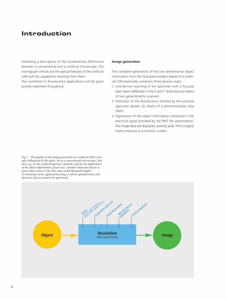
Fig. 1 The quality of the image generated in a confocal LSM is not only influenced by the optics (as in a conventional microscope), but also, e.g., by the confocal aperture (pinhole) and by the digitization of the object information (pixel size). Another important factor is noise (laser noise, or the shot noise of the fluorescent light). To minimize noise, signal-processing as well as optoelectronic and electronic devices need to be optimized.

Introduction

Following a description of the fundamental differences

between a conventional and a confocal microscope, this

monograph will set out the special features of the confocal

LSM and the capabilities resulting from them.

The conditions in fluorescence applications will be given

priority treatment throughout.

Image�generation

The complete generation of the two-dimensional object

information from the focal plane (object plane) of a confo-

cal LSM essentially comprises three process steps:

1. Line-by-line scanning of the specimen with a focused

laser beam deflected in the X and Y directions by means

of two galvanometric scanners.

2. Detection of the fluorescence emitted by the scanned

specimen details, by means of a photomultiplier tube

(PMT).

3. Digitization of the object information contained in the

electrical signal provided by the PMT (for presentation,

the image data are displayed, pixel by pixel, from a digital

matrix memory to a monitor screen).

Object ResolutionIdeal optical theory Image

Digitizati

on pixel si

ze

Pupil illuminati

on

Resudial

optical

abera

tions

Confocal ap

erture

Noise

Detecto

r, lase

r, elec

tronics

,

photons (light; q

uantum noise

)

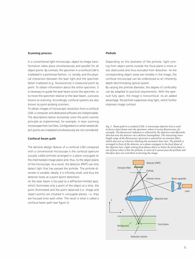
Scanning�process

In a conventional light microscope, object-to-image trans-

formation takes place simultaneously and parallel for all

object points. By contrast, the specimen in a confocal LSM is

irradiated in a pointwise fashion, i.e. serially, and the physi-

cal inter action between the laser light and the specimen

detail irradiated (e.g. fluorescence) is measured point by

point. To obtain information about the entire specimen, it

is necessary to guide the laser beam across the specimen, or

to move the specimen relative to the laser beam, a process

known as scanning. Accordingly, confocal systems are also

known as point-probing scanners.

To obtain images of microscopic resolution from a confocal

LSM, a computer and dedicated software are indispensable.

The descriptions below exclusively cover the point scanner

principle as implemented, for example, in laser scanning

microscopes from Carl Zeiss. Configurations in which several ob-

ject points are irradiated simultaneously are not considered.

Confocal�beam�path

The decisive design feature of a confocal LSM compared

with a conventional microscope is the confocal aperture

(usually called pinhole) arranged in a plane conjugate to

the intermediate image plane and, thus, to the object plane

of the microscope. As a result, the detector (PMT) can only

detect light that has passed the pinhole. The pinhole di-

ameter is variable; ideally, it is infinitely small, and thus the

detector looks at a point (point detection).

As the laser beam is focused to a diffraction-limited spot,

which illuminates only a point of the object at a time, the

point illuminated and the point observed (i.e. image and

object points) are situated in conjugate planes, i.e. they

are focused onto each other. The result is what is called a

confocal beam path (see figure 2).

5

Fig. 2 Beam path in a confocal LSM. A microscope objective lens is used to focus a laser beam onto the specimen, where it excites fluorescence, for example. The fluorescent radiation is collected by the objective and efficiently directed onto the detector via a dichroic beamsplitter. The interesting wave-length range of the fluorescence spectrum is selected by an emission filter, which also acts as a barrier, blocking the excitation laser line. The pinhole is arranged in front of the detector, on a plane conjugate to the focal plane of the objective lens. Light coming from planes above or below the focal plane is out of focus when it hits the pinhole, so most of it cannot pass the pinhole and therefore does not contribute to forming the image.

Pinhole

Depending on the diameter of the pinhole, light com-

ing from object points outside the focal plane is more or

less obstructed and thus excluded from detection. As the

corresponding object areas are invisible in the image, the

confocal microscope can be understood as an inherently

depth-discriminating optical system.

By varying the pinhole diameter, the degree of confocality

can be adapted to practical requirements. With the aper-

ture fully open, the image is nonconfocal. As an added

advantage, the pinhole suppresses stray light, which further

improves image contrast.

X

Z

Detector (PMT)

PinholeEmission filter

Dichroic mirror

Focal plane

Objective lens

Detection volume

Background

Beam expander

Laser

6

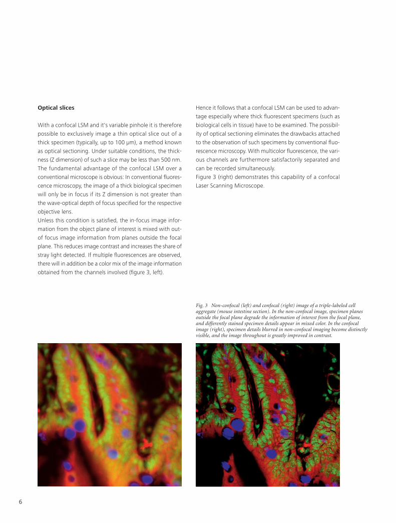
Fig. 3 Non-confocal (left) and confocal (right) image of a triple-labeled cell aggregate (mouse intestine section). In the non-confocal image, specimen planes outside the focal plane degrade the information of interest from the focal plane, and differently stained specimen details appear in mixed color. In the confocal image (right), specimen details blurred in non-confocal imaging become distinctly visible, and the image throughout is greatly improved in contrast.

Optical�slices

With a confocal LSM and it's variable pinhole it is therefore

possible to exclusively image a thin optical slice out of a

thick specimen (typically, up to 100 µm), a method known

as optical sectioning. Under suitable conditions, the thick-

ness (Z dimension) of such a slice may be less than 500 nm.

The fundamental advantage of the confocal LSM over a

conventional microscope is obvious: In conventional fluores-

cence microscopy, the image of a thick biological specimen

will only be in focus if its Z dimension is not greater than

the wave-optical depth of focus specified for the respective

objective lens.

Unless this condition is satisfied, the in-focus image infor-

mation from the object plane of interest is mixed with out-

of focus image information from planes outside the focal

plane. This reduces image contrast and increases the share of

stray light detected. If multiple fluorescences are observed,

there will in addition be a color mix of the image information

obtained from the channels involved (figure 3, left).

Hence it follows that a confocal LSM can be used to advan-

tage especially where thick fluorescent specimens (such as

biological cells in tissue) have to be examined. The possibil-

ity of optical sectioning eliminates the drawbacks attached

to the obser vation of such specimens by conventional fluo-

rescence microscopy. With multicolor fluorescence, the vari-

ous channels are furthermore satisfactorily separated and

can be recorded simultaneously.

Figure 3 (right) demonstrates this capability of a confocal

Laser Scanning Microscope.

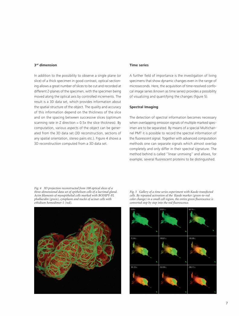
3rd�dimension

In addition to the possibility to observe a single plane (or

slice) of a thick specimen in good contrast, optical section-

ing allows a great number of slices to be cut and recorded at

different Z-planes of the specimen, with the specimen being

moved along the optical axis by controlled increments. The

result is a 3D data set, which provides information about

the spatial structure of the object. The quality and accuracy

of this information depend on the thickness of the slice

and on the spacing between successive slices (optimum

scanning rate in Z direction = 0.5x the slice thickness). By

computation, various aspects of the object can be gener-

ated from the 3D data set (3D reconstruction, sections of

any spatial orientation, stereo pairs etc.). Figure 4 shows a

3D reconstruction computed from a 3D data set.

7

Fig. 4 3D projection reconstructed from 108 optical slices of a three-dimensional data set of epithelium cells of a lacrimal gland. Actin filaments of myoepithelial cells marked with BODIPY-FL phallacidin (green), cytoplasm and nuclei of acinar cells with ethidium homodimer-1 (red).

Fig. 5 Gallery of a time series experiment with Kaede-transfected cells. By repeated activation of the Kaede marker (green-to-red color change) in a small cell region, the entire green fluorescence is converted step by step into the red fluorescence.

Time�series

A further field of importance is the investigation of living

specimens that show dynamic changes even in the range of

microseconds. Here, the acquisition of time-resolved confo-

cal image series (known as time series) provides a possibility

of visualizing and quantifying the changes (figure 5).

Spectral�Imaging

The detection of spectral information becomes necessary

when overlapping emission signals of multiple marked spec-

imen are to be separated. By means of a special Multichan-

nel PMT it is possible to record the spectral information of

the fluorescent signal. Together with advanced computation

methods one can separate signals which almost overlap

completely and only differ in their spectral signature. The

method behind is called ‘’linear unmixing’’ and allows, for

example, several fluorescent proteins to be distinguished.

0.00 s 28.87 s 64.14 s

72.54 s 108.81 s 145.08 s

181.35 s 253.90 s 290.17 s

8

Point Spread Function

In order to understand the optical performance charac-

teristics of a confocal LSM in detail, it is necessary to have

a closer look at the fundamental optical phenomena re-

sulting from the geometry of the confocal beam path. As

mentioned before, what is most essential about a confocal

LSM is that both illumination and observation (detection)

are limited to a point.

Not even an optical system of diffraction-limited design

can image a truly point-like object as a point. The image

of an ideal point object will always be somewhat blurred,

or “spread” corresponding to the imaging properties of

the optical system. The image of a point can be described

in quantitative terms by the point spread function (PSF),

which maps the intensity distribution in the image space.

Where the three-dimensional imaging properties of a con-

focal LSM are concerned, it is necessary to consider the

3D-PSF.

In the ideal, diffraction-limited case (no optical aberrations,

and homogeneous illumination at all lens cross sections –

see Part 3 “Pupil Illumination”), the 3D-PSF is of comet-like,

rotationally symmetrical shape.

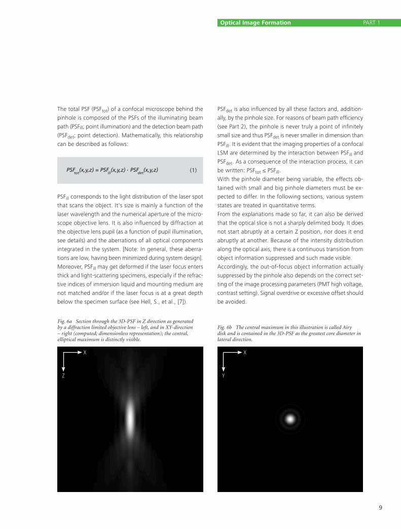
For illustration, Figure 6 shows two-dimensional sections

(XZ and XY) through an ideal 3D-PSF.

From the illustration it is evident that the central maximum

of the 3D-PSF, in which 86.5% of the total energy available

in the pupil of the objective lens are concentrated, can be

described as an ellipsoid of rotation. For considerations of

resolution and optical slice thickness it is useful to define

the half-maximum area of the ellipsoid, i.e. the well-defined

area in which the intensity of the 3D PSF in axial and lateral

direction has dropped to half of the central maximum.

Any reference to the PSF in the following discussion exclu-

sively refers to the half-maximum area.

As said before the confocal LSM system as a whole gen-

erates two point images: one by projecting a point light

source into the object space, the other by projecting a point

detail of the object into the image space.

The total PSF (PSFtot) of a confocal microscope behind the

pinhole is composed of the PSFs of the illuminating beam

path (PSFill; point illumination) and the detection beam path

(PSFdet; point detection). Mathematically, this relationship

can be described as follows:

PSFill corresponds to the light distribution of the laser spot

that scans the object. It's size is mainly a function of the

laser wavelength and the numerical aperture of the micro-

scope objective lens. It is also influenced by diffraction at

the objective lens pupil (as a function of pupil illumination,

see details) and the aberrations of all optical components

integrated in the system. [Note: In general, these aberra-

tions are low, having been minimized during system design].

Moreover, PSFill may get deformed if the laser focus enters

thick and light-scattering specimens, especially if the refrac-

tive indices of immersion liquid and mounting medium are

not matched and/or if the laser focus is at a great depth

below the specimen surface (see Hell, S., et al., [7]).

9

Fig. 6a Section through the 3D-PSF in Z direction as generated by a diffraction limited objective lens – left, and in XY-direction – right (computed; dimensionless representation); the central, elliptical maximum is distinctly visible.

Optical�Image�Formation PART 1

seite 7

PSFtot

(x,y,z) = PSFill

(x,y,z) . PSFdet

(x,y,z)

seite 9

FWHMill,axial =

seite 11

FWHMdet,axial =0.88 . em

n- n2-NA2+

2 . n . PHNA

2 2

0.88 . exc

(n- n2-NA2)

1.77 . n . exc

NA2

FWHMill,lateral = 0.51 exc

NA

seite 12

PSFtot

(x,y,z) = (PSFill

(x,y,z))2

em .

exc2exc + 2

em

2

FWHMtot,axial = 0.64 .

(n- n2-NA2)

1.28 . n .

NA2

FWHMtot,lateral = 0.37NA

(1)

X

Z

X

Y

PSFdet is also influenced by all these factors and, addition-

ally, by the pinhole size. For reasons of beam path efficiency

(see Part 2), the pinhole is never truly a point of infinitely

small size and thus PSFdet is never smaller in dimension than

PSFill. It is evident that the imaging properties of a confocal

LSM are determined by the interaction between PSFill and

PSFdet. As a consequence of the interaction process, it can

be written: PSFtot ≤ PSFill.

With the pinhole diameter being variable, the effects ob-

tained with small and big pinhole diameters must be ex-

pected to differ. In the following sections, various system

states are treated in quantitative terms.

From the explanations made so far, it can also be derived

that the optical slice is not a sharply delimited body. It does

not start abruptly at a certain Z position, nor does it end

abruptly at another. Because of the intensity distribution

along the optical axis, there is a continuous transition from

object information suppressed and such made visible.

Accordingly, the out-of-focus object information actually

suppressed by the pinhole also depends on the correct set-

ting of the image processing parameters (PMT high voltage,

contrast setting). Signal overdrive or excessive offset should

be avoided.

Fig. 6b The central maximum in this illustration is called Airy disk and is contained in the 3D-PSF as the greatest core diameter in lateral direction.

10

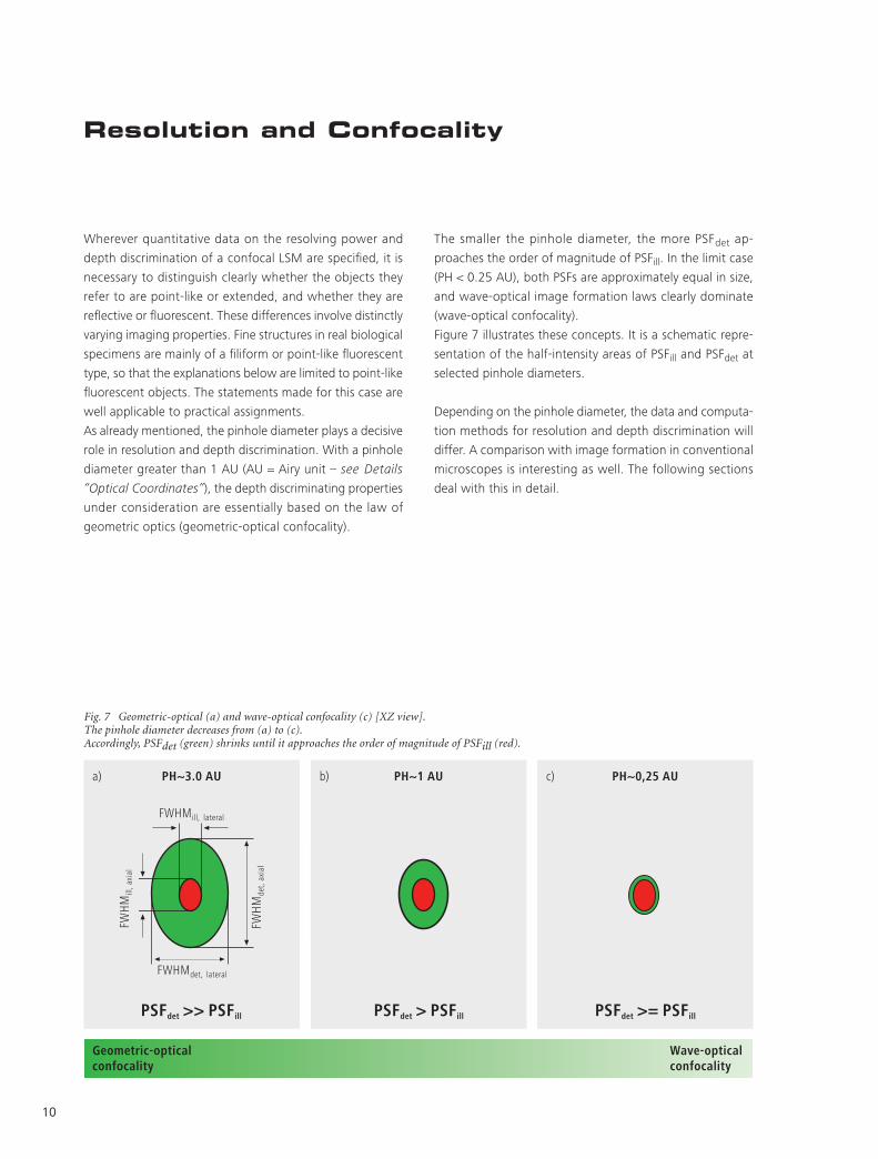
Fig. 7 Geometric-optical (a) and wave-optical confocality (c) [XZ view]. The pinhole diameter decreases from (a) to (c).Accordingly, PSFdet (green) shrinks until it approaches the order of magnitude of PSFill (red).

Resolution and Confocality

Wherever quantitative data on the resolving power and

depth discrimination of a confocal LSM are specified, it is

necessary to distinguish clearly whether the objects they

refer to are point-like or extended, and whether they are

reflective or fluorescent. These differences involve distinctly

varying imaging properties. Fine structures in real biological

specimens are mainly of a filiform or point-like fluorescent

type, so that the explanations below are limited to point-like

fluorescent objects. The statements made for this case are

well applicable to practical assignments.

As already mentioned, the pinhole diameter plays a decisive

role in resolution and depth discrimination. With a pinhole

diameter greater than 1 AU (AU = Airy unit – see Details

“Optical Coordinates”), the depth discriminating properties

under consideration are essentially based on the law of

geometric optics (geometric-optical confocality).

The smaller the pinhole diameter, the more PSFdet ap-

proaches the order of magnitude of PSFill. In the limit case

(PH < 0.25 AU), both PSFs are approximately equal in size,

and wave-optical image formation laws clearly dominate

(wave-optical confocality).

Figure 7 illustrates these concepts. It is a schematic repre-

sentation of the half-intensity areas of PSFill and PSFdet at

selected pinhole diameters.

Depending on the pinhole diameter, the data and computa-

tion methods for resolution and depth discrimination will

differ. A comparison with image formation in conventional

microscopes is interesting as well. The following sections

deal with this in detail.

a) PH~3.0 AU

PSFdet > PSFill

b)

PSFdet >= PSFill

c)

Geometric-opticalconfocality

Wave-opticalconfocality

PH~1 AU PH~0,25 AU

FWH

Mde

t, ax

ial

FWHMill, lateral

FWH

Mill

, axi

al

PSFdet >> PSFill

FWHMdet, lateral

Resolution

Resolution, in case of large pinhole diameters (PH >1AU),

is meant to express the separate visibility, both laterally

and axially, of points during the scanning process. Imagine

an object consisting of individual points: all points spaced

closer than the extension of PSFill are blurred (spread), i.e.

they are not resolved.

Quantitatively, resolution results from the axial and lateral

extension of the scanning laser spot, or the elliptical half-

intensity area of PSFill. On the assumption of homogeneous

pupil illumination, the following equations apply:

11

At first glance, equations (2a) and (3) are not different from

those known for conventional imaging (see Beyer, H., [1]).

It is striking, however, that the resolving power in the con-

focal microscope depends only on the wavelength of the

illuminating light, rather than exclusively on the emission

wavelength as in the conventional case.

Compared to the conventional fluorescence microscope,

confocal fluorescence with large pinhole diameters leads to

a gain in resolution by the factor (λem/λexc) via the stokes

shift.

If NA < 0.5, equation (2) can be approximated by:

seite 7

PSFtot

(x,y,z) = PSFill

(x,y,z) . PSFdet

(x,y,z)

seite 9

FWHMill,axial =

seite 11


n- n2-NA2+

2 . n . PHNA

2 2

0.88 . exc

(n- n2-NA2)

1.77 . n . exc

NA2


NA

seite 12

PSFtot

(x,y,z) = (PSFill

(x,y,z))2

em .

exc2exc + 2

em

2


(n- n2-NA2)

1.28 . n .

NA2


(2a)

Lateral:

seite 7

PSFtot

(x,y,z) = PSFill

(x,y,z) . PSFdet

(x,y,z)

seite 9

FWHMill,axial =

seite 11


n- n2-NA2+

2 . n . PHNA

2 2

0.88 . exc

(n- n2-NA2)

1.77 . n . exc

NA2


NA

seite 12

PSFtot

(x,y,z) = (PSFill

(x,y,z))2

em .

exc2exc + 2

em

2


(n- n2-NA2)

1.28 . n .

NA2


(3)

Axial:

seite 7

PSFtot

(x,y,z) = PSFill

(x,y,z) . PSFdet

(x,y,z)

seite 9

FWHMill,axial =

seite 11


n- n2-NA2+

2 . n . PHNA

2 2

0.88 . exc

(n- n2-NA2)

1.77 . n . exc

NA2


NA

seite 12

PSFtot

(x,y,z) = (PSFill

(x,y,z))2

em .

exc2exc + 2

em

2


(n- n2-NA2)

1.28 . n .

NA2


(2)

n = refractive index of immersion liquid NA = numerical aperture of the objectiveλexc = wavelength of the excitation light


12

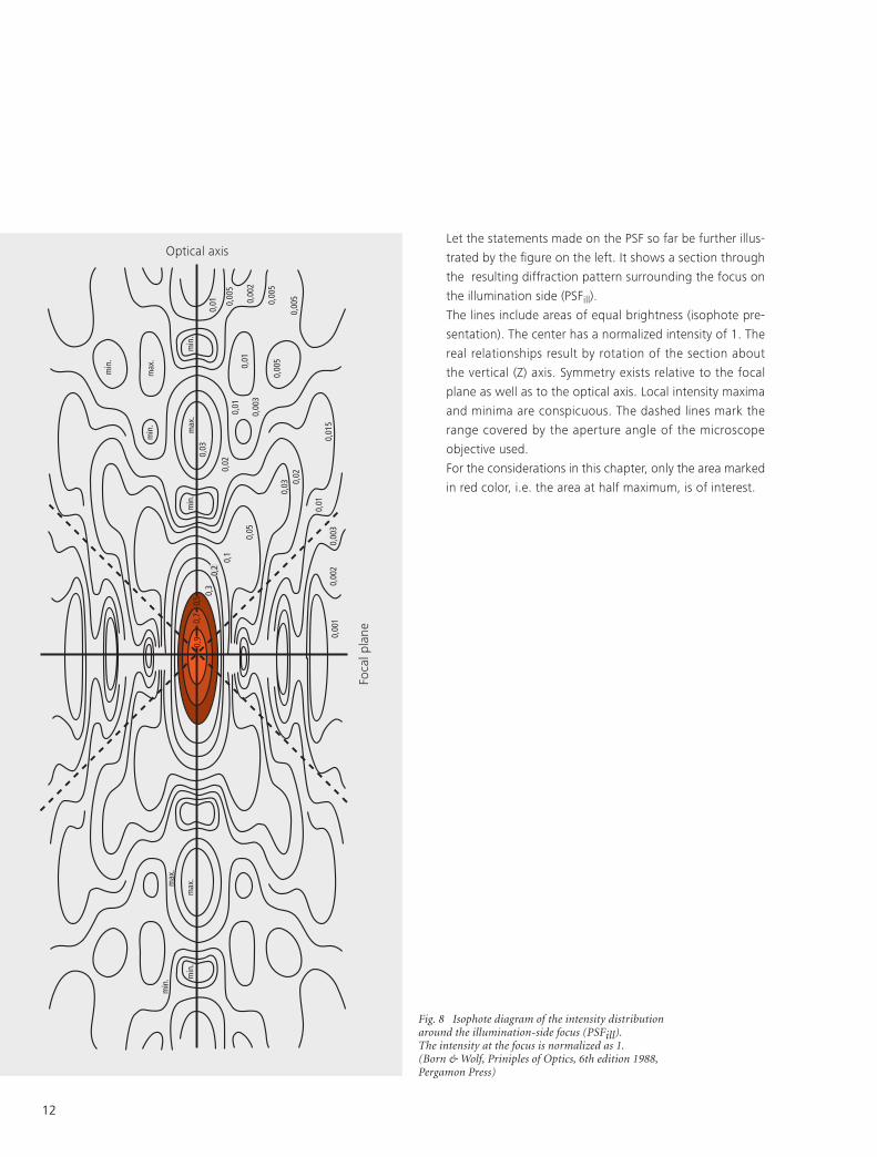
Fig. 8 Isophote diagram of the intensity distribution around the illumination-side focus (PSFill). The intensity at the focus is normalized as 1.(Born & Wolf, Priniples of Optics, 6th edition 1988, Pergamon Press)

Let the statements made on the PSF so far be further illus-

trated by the figure on the left. It shows a section through

the resulting diffraction pattern surrounding the focus on

the illumination side (PSFill).

The lines include areas of equal brightness (isophote pre-

sentation). The center has a normalized intensity of 1. The

real relationships result by rotation of the section about

the vertical (Z) axis. Symmetry exists relative to the focal

plane as well as to the optical axis. Local intensity maxima

and minima are conspicuous. The dashed lines mark the

range covered by the aperture angle of the microscope

objective used.

For the considerations in this chapter, only the area marked

in red color, i.e. the area at half maximum, is of interest.

min

.m

ax.

min

.m

ax.

0,9

0,7

0,5

0,3

0,2

0,1

0,05

0,03 0,

02

0,01

50,

01

0,00

30,

002

0,00

1

min

.m

ax.

min

.

min

.

min

.

max

.

0,03

0,01

0,00

3

0,02

0,00

5

0,01

0,00

50,00

5

0,00

2

0,00

5

0,01

Optical axis

Foca

l pla

ne

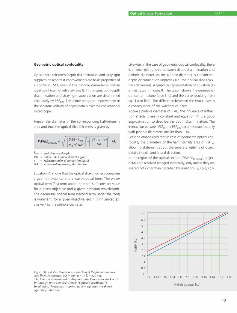
Geometric�optical�confocality

Optical slice thickness (depth discrimination) and stray light

suppression (contrast improvement) are basic properties of

a confocal LSM, even if the pinhole diameter is not an

ideal point (i.e. not infinitely small). In this case, both depth

discrimination and stray light suppression are determined

exclusively by PSFdet. This alone brings an improvement in

the separate visibility of object details over the conventional

microscope.

Hence, the diameter of the corresponding half-intensity

area and thus the optical slice thickness is given by:

Equation (4) shows that the optical slice thickness comprises

a geometric-optical and a wave-optical term. The wave-

optical term (first term under the root) is of constant value

for a given objective and a given emission wavelength.

The geometric-optical term (second term under the root)

is dominant; for a given objective lens it is influenced ex-

clusively by the pinhole diameter.

13

Fig.9 Optical slice thickness as a function of the pinhole diameter (red line). Parameters: NA = 0.6; n = 1; λ = 520 nm. The X axis is dimensioned in Airy units, the Y axis (slice thickness) in Rayleigh units (see also: Details “Optical Coordinates”). In addition, the geometric-optical term in equation 4 is shown separately (blue line).

λem = emission wavelength PH = object-side pinhole diameter [µm] n = refractive index of immersion liquid NA = numerical aperture of the objective

Likewise, in the case of geometric-optical confocality, there

is a linear relationship between depth discrimination and

pinhole diameter. As the pinhole diameter is constricted,

depth discrimination improves (i.e. the optical slice thick-

ness decreases). A graphical representation of equation (4)

is illustrated in figure 9. The graph shows the geometric-

optical term alone (blue line) and the curve resulting from

eq. 4 (red line). The difference between the two curves is

a consequence of the waveoptical term.

Above a pinhole diameter of 1 AU, the influence of diffrac-

tion effects is nearly constant and equation (4) is a good

approximation to describe the depth discrimination. The

interaction between PSFill and PSFdet becomes manifest only

with pinhole diameters smaller than 1 AU.

Let it be emphasized that in case of geometric optical con-

focality the diameters of the half-inten sity area of PSFdet

allow no statement about the separate visibility of object

details in axial and lateral direction.

In the region of the optical section (FWHMdet,axial), object

details are resolved (imaged separately) only unless they are

spaced not closer than described by equations (2) / (2a) / (3).

seite 7

PSFtot

(x,y,z) = PSFill

(x,y,z) . PSFdet

(x,y,z)

seite 9

FWHMill,axial =

seite 11


n- n2-NA2+

2 . n . PHNA

2 2

0.88 . exc

(n- n2-NA2)

1.77 . n . exc

NA2


NA

seite 12

PSFtot

(x,y,z) = (PSFill

(x,y,z))2

em .

exc2exc + 2

em

2


(n- n2-NA2)

1.28 . n .

NA2


(4)

FWH

M [R

U]

Pinhole diameter [AU]

7.0

6.3

5.6

4.9

4.2

3.5

2.8

2.1

1.4

0.7

01.2 1.48 1.76 2.04 2.32 2.6 2.88 3.16 3.44 3.72 4.0


Thus, equations (2) and (3) for the widths of the axial and

lateral half-intensity areas are transformed into:

14

1 For rough estimates, the expression λ ≈ √λem·λexc suffices.

Wave-optical�confocality

If the pinhole is closed down to a diameter of <0.25 AU (vir-

tually “infinitely small”), the character of the image changes.

Additional diffraction effects at the pinhole have to be taken

into account, and PSFdet (optical slice thickness) shrinks

to the order of magnitude of PSFill (Z resolution) (see also

figure 7c).

In order to achieve simple formulae for the range of smallest

pinhole diameters, it is practical to regard the limit of PH = 0

at first, even though it is of no practical use. In this case,

PSFdet and PSFill are identical. The total PSF can be written as:

In fluorescence applications it is furthermore necessary to

consider both the excitation wavelength λexc and the emis-

sion wavelength λem. This is done by specifying a mean

wavelength1:

seite 7

PSFtot

(x,y,z) = PSFill

(x,y,z) . PSFdet

(x,y,z)

seite 9

FWHMill,axial =

seite 11


n- n2-NA2+

2 . n . PHNA

2 2

0.88 . exc

(n- n2-NA2)

1.77 . n . exc

NA2


NA

seite 12

PSFtot

(x,y,z) = (PSFill

(x,y,z))2

em .

exc2exc + 2

em

2


(n- n2-NA2)

1.28 . n .

NA2


(5)

seite 7

PSFtot

(x,y,z) = PSFill

(x,y,z) . PSFdet

(x,y,z)

seite 9

FWHMill,axial =

seite 11


n- n2-NA2+

2 . n . PHNA

2 2

0.88 . exc

(n- n2-NA2)

1.77 . n . exc

NA2


NA

seite 12

PSFtot

(x,y,z) = (PSFill

(x,y,z))2

em .

exc2exc + 2

em

2


(n- n2-NA2)

1.28 . n .

NA2


(6)

Note:

With�the�object�being�a�mirror,�the�factor�in�equa-

tion�7�is�0.45�(instead�of�0.64),�and�0.88�(instead�of�

1.28)�in�equation�7a.�For�a�fluorescent�plane�of�finite�

thickness,�a�factor�of�0.7�can�be�used�in�equation�7.�

This�underlines�that�apart�from�the�parameters�(NA,�

λ,�n)�influencing�the�optical�slice�thickness,�the�type�

of�specimen�also�affects�the�measurement�result.

seite 7

PSFtot

(x,y,z) = PSFill

(x,y,z) . PSFdet

(x,y,z)

seite 9

FWHMill,axial =

seite 11


n- n2-NA2+

2 . n . PHNA

2 2

0.88 . exc

(n- n2-NA2)

1.77 . n . exc

NA2


NA

seite 12

PSFtot

(x,y,z) = (PSFill

(x,y,z))2

em .

exc2exc + 2

em

2


(n- n2-NA2)

1.28 . n .

NA2


(7)

seite 7

PSFtot

(x,y,z) = PSFill

(x,y,z) . PSFdet

(x,y,z)

seite 9

FWHMill,axial =

seite 11


n- n2-NA2+

2 . n . PHNA

2 2

0.88 . exc

(n- n2-NA2)

1.77 . n . exc

NA2


NA

seite 12

PSFtot

(x,y,z) = (PSFill

(x,y,z))2

em .

exc2exc + 2

em

2


(n- n2-NA2)

1.28 . n .

NA2

FWHMtot,lateral = 0.37NA (8)

seite 7

PSFtot

(x,y,z) = PSFill

(x,y,z) . PSFdet

(x,y,z)

seite 9

FWHMill,axial =

seite 11


n- n2-NA2+

2 . n . PHNA

2 2

0.88 . exc

(n- n2-NA2)

1.77 . n . exc

NA2


NA

seite 12

PSFtot

(x,y,z) = (PSFill

(x,y,z))2

em .

exc2exc + 2

em

2


(n- n2-NA2)

1.28 . n .

NA2


(7a)

Axial:

If NA < 0.5, equation (2) can be approximated by:

Lateral:

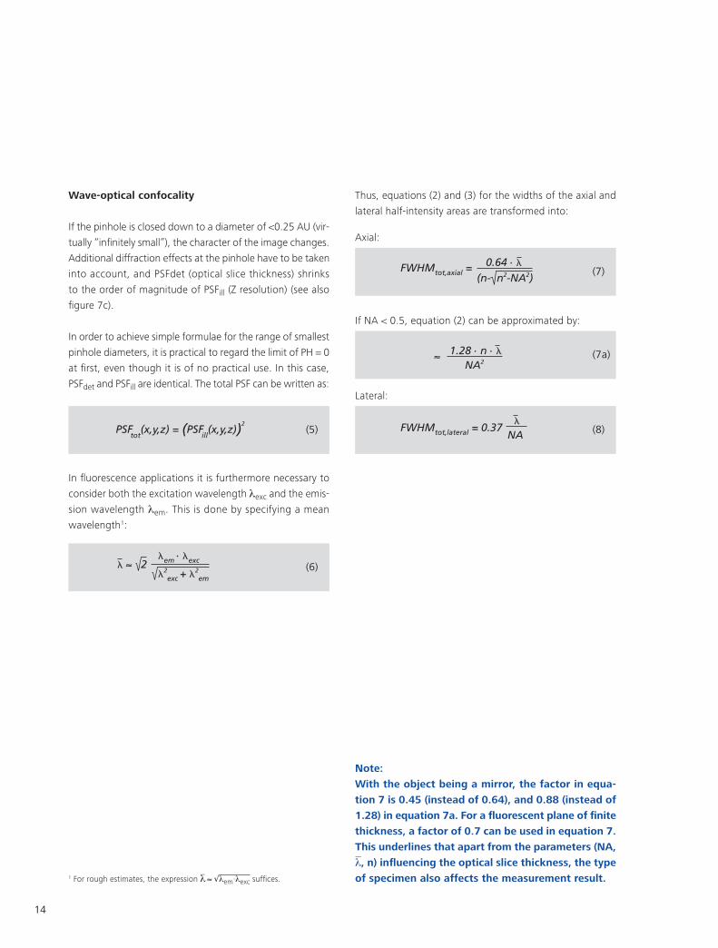
From equations (7) and (7a) it is evident that depth resolu-

tion varies linearly with the refractive index n of the immer-

sion liquid and with the square of the inverse value of the

numerical aperture of the objective lens {NA = n · sin(α)}.

To achieve high depth discrimination, it is important, above

all, to use objective lenses with the highest possible numeri-

cal aperture.

As an NA > 1 can only be obtained with an immersion liquid,

confocal fluorescence microscopy is usually performed with

immersion objectives (see also figure 11).

A comparison of the results stated before shows that axial

and lateral resolution in the limit case of PH=0 can be im-

proved by a factor of 1.4. Furthermore it should be noted

that, because of the wave-optical relationships discussed,

the optical performance of a confocal LSM cannot be en-

hanced infinitely. Equations (7) and (8) supply the minimum

possible slice thickness and the best possible resolution,

respectively.

15

From the applications point of view, the case of strictly

wave-optical confocality (PH=0) is irrelevant (see also Part 2).

By merely changing the factors in equations (7) and (8) it

is possible, though, to transfer the equations derived for

PH=0 to the pinhole diameter range up to 1 AU, to a good

approximation. The factors applicable to particular pinhole

diameters can be taken from figure 10.

It must also be noted that with PH <1AU, a distinction be-

tween optical slice thickness and resolution can no longer

be made. The thickness of the optical slice at the same time

specifies the resolution properties of the system. That is why

in the literature the term of depth resolution is frequently

used as a synonym for depth discrimination or optical slice

thickness. However, this is only correct for pinhole diam-

eters smaller than 1 AU.

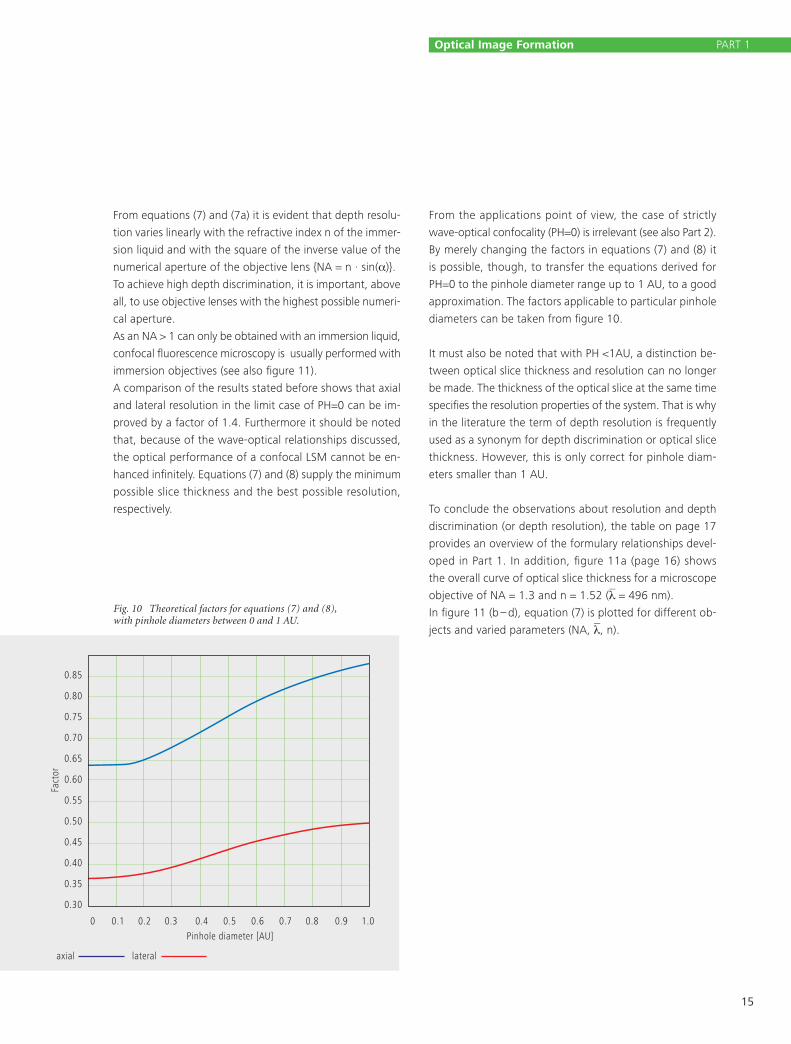
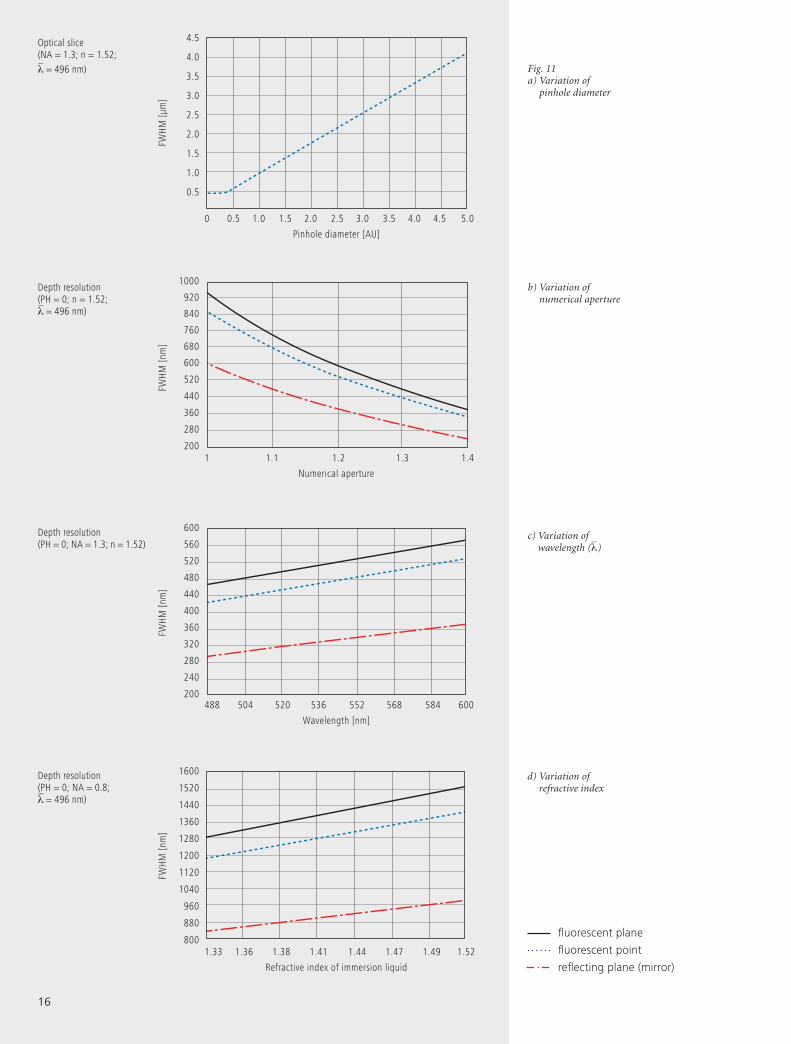
To conclude the observations about resolution and depth

discrimination (or depth resolution), the table on page 17

provides an overview of the formulary relationships devel-

oped in Part 1. In addition, figure 11a (page 16) shows

the overall curve of optical slice thickness for a microscope

objective of NA = 1.3 and n = 1.52 (λ = 496 nm).

In figure 11 (b – d), equation (7) is plotted for different ob-

jects and varied parameters (NA, λ, n).


Fact

or

0.85

0.80

0.75

0.70

0.65

0.60

0.55

0.50

0.45

0.40

0.35

0.30

0 0.1 0.2 0.3 0.4 0.5 0.6 0.7 0.8 0.9 1.0

axial lateral

Fig. 10 Theoretical factors for equations (7) and (8), with pinhole diameters between 0 and 1 AU.


16

Fig. 11a) Variation of

pinhole diameter

b) Variation of numerical aperture

d) Variation of refractive index

c) Variation of wavelength (λ)

fluorescent plane

fluorescent point

reflecting plane (mirror)

Optical slice(NA = 1.3; n = 1.52; λ = 496 nm)

4.5

4.0

3.5

3.0

2.5

2.0

1.5

1.0

0.5

0 0.5 1.0 1.5 2.0 2.5 3.0 3.5 4.0 4.5 5.0


FWH

M [µ

m]

Depth resolution(PH = 0; n = 1.52; λ = 496 nm)

1000

920

840

760

680

600

520

440

360

280

200

600

560

520

480

440

400

360

320

280

240

200

1 1.1 1.2 1.3 1.4

Numerical aperture

FWH

M [n

m]

Depth resolution(PH = 0; NA = 1.3; n = 1.52)

488 504 520 536 552 568 584 600

Wavelength [nm]

FWH

M [n

m]

Depth resolution(PH = 0; NA = 0.8; λ = 496 nm)

1600

1520

1440

1360

1280

1200

1120

1040

960

880

8001.33 1.36 1.38 1.41 1.44 1.47 1.49 1.52

Refractive index of immersion liquid

FWH

M [n

m]

17

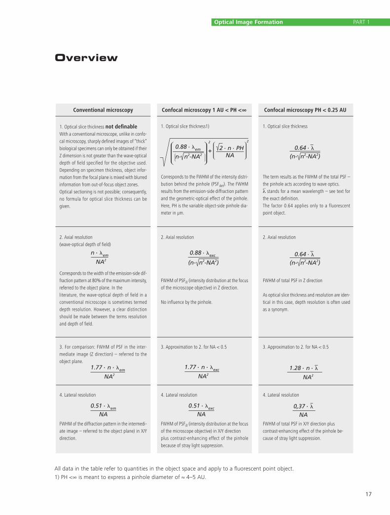
Overview

All data in the table refer to quantities in the object space and apply to a fluorescent point object.

1) PH <∞ is meant to express a pinhole diameter of ≈ 4–5 AU.

Conventional microscopy

1. Optical slice thickness not definableWith a conventional microscope, unlike in confo-cal microscopy, sharply defined images of “thick” biological specimens can only be obtained if their Z dimension is not greater than the wave-optical depth of field specified for the objective used. Depending on specimen thickness, object infor-mation from the focal plane is mixed with blurred information from out-of-focus object zones.Optical sectioning is not possible; consequently, no formula for optical slice thickness can be given.

1. Optical slice thickness1)

Corresponds to the FWHM of the intensity distri-bution behind the pinhole (PSFdet). The FWHM results from the emission-side diffraction pattern and the geometric- optical effect of the pinhole. Here, PH is the variable object-side pinhole dia-meter in µm.

1. Optical slice thickness

The term results as the FWHM of the total PSF – the pinhole acts according to wave optics.λ stands for a mean wavelength – see text for the exact definition.The factor 0.64 applies only to a fluorescent point object.

2. Axial resolution (wave-optical depth of field)

Corresponds to the width of the emission-side dif-fraction pattern at 80% of the maximum intensity, referred to the object plane. In the literature, the wave-optical depth of field in a conventional microscope is sometimes termed depth resolution. However, a clear distinction should be made between the terms resolution and depth of field.

2. Axial resolution

FWHM of PSFill (intensity distribution at the focus of the microscope objective) in Z direction.

No influence by the pinhole.

2. Axial resolution

FWHM of total PSF in Z direction

As optical slice thickness and resolution are iden-tical in this case, depth resolution is often used as a synonym.

3. For comparison: FWHM of PSF in the inter-mediate image (Z direction) – referred to the object plane.

3. Approximation to 2. for NA < 0.5 3. Approximation to 2. for NA < 0.5

4. Lateral resolution

FWHM of the diffraction pattern in the intermedi-ate image – referred to the object plane) in X/Y direction.


FWHM of PSFill (intensity distribution at the focus of the microscope objective) in X/Y direction plus contrast-enhancing effect of the pinhole because of stray light suppression.


FWHM of total PSF in X/Y direction plus contrast-enhancing effect of the pinhole be-cause of stray light suppression.

Confocal microscopy 1 AU < PH <∞ Confocal microscopy PH < 0.25 AU


seite 15

0.88 . �em

n- n2-NA2+ 2 . n . PH

NA

2 2 0.64 . �

(n- n2-NA2)

0.64 . �

(n- n2-NA2)

0.88 . �exc

(n- n2-NA2)

n . �em

NA2

1.77 . n . �em

NA2

0.51 . �em

NA

1.77 . n . �exc

NA2

1.28 . n . �NA2

0,37 . �NA

0.51 . �exc

NA

seite 19

system constant

number of pixels . zoomfactor . magnificationobj

dpix =

3.92 . NA . system constant

number of pixels .magnificationobj . �exc

Z ≥

seite 15

0.88 . �em

n- n2-NA2+ 2 . n . PH

NA

2 2 0.64 . �

(n- n2-NA2)

0.64 . �

(n- n2-NA2)

0.88 . �exc

(n- n2-NA2)

n . �em

NA2

1.77 . n . �em

NA2

0.51 . �em

NA

1.77 . n . �exc

NA2

1.28 . n . �NA2

0,37 . �NA

0.51 . �exc

NA

seite 19

system constant


dpix =



Z ≥

seite 15

0.88 . �em

n- n2-NA2+ 2 . n . PH

NA

2 2 0.64 . �

(n- n2-NA2)

0.64 . �

(n- n2-NA2)

0.88 . �exc

(n- n2-NA2)

n . �em

NA2

1.77 . n . �em

NA2

0.51 . �em

NA

1.77 . n . �exc

NA2

1.28 . n . �NA2

0,37 . �NA

0.51 . �exc

NA

seite 19

system constant


dpix =



Z ≥

seite 15

0.88 . �em

n- n2-NA2+ 2 . n . PH

NA

2 2 0.64 . �

(n- n2-NA2)

0.64 . �

(n- n2-NA2)

0.88 . �exc

(n- n2-NA2)

n . �em

NA2

1.77 . n . �em

NA2

0.51 . �em

NA

1.77 . n . �exc

NA2

1.28 . n . �NA2

0,37 . �NA

0.51 . �exc

NA

seite 19

system constant


dpix =



Z ≥

seite 15

0.88 . �em

n- n2-NA2+ 2 . n . PH

NA

2 2 0.64 . �

(n- n2-NA2)

0.64 . �

(n- n2-NA2)

0.88 . �exc

(n- n2-NA2)

n . �em

NA2

1.77 . n . �em

NA2

0.51 . �em

NA

1.77 . n . �exc

NA2

1.28 . n . �NA2

0,37 . �NA

0.51 . �exc

NA

seite 19

system constant


dpix =



Z ≥

seite 15

0.88 . �em

n- n2-NA2+ 2 . n . PH

NA

2 2 0.64 . �

(n- n2-NA2)

0.64 . �

(n- n2-NA2)

0.88 . �exc

(n- n2-NA2)

n . �em

NA2

1.77 . n . �em

NA2

0.51 . �em

NA

1.77 . n . �exc

NA2

1.28 . n . �NA2

0,37 . �NA

0.51 . �exc

NA

seite 19

system constant


dpix =



Z ≥

seite 15

0.88 . �em

n- n2-NA2+ 2 . n . PH

NA

2 2 0.64 . �

(n- n2-NA2)

0.64 . �

(n- n2-NA2)

0.88 . �exc

(n- n2-NA2)

n . �em

NA2

1.77 . n . �em

NA2

0.51 . �em

NA

1.77 . n . �exc

NA2

1.28 . n . �NA2

0,37 . �NA

0.51 . �exc

NA

seite 19

system constant


dpix =



Z ≥

seite 15

0.88 . �em

n- n2-NA2+ 2 . n . PH

NA

2 2 0.64 . �

(n- n2-NA2)

0.64 . �

(n- n2-NA2)

0.88 . �exc

(n- n2-NA2)

n . �em

NA2

1.77 . n . �em

NA2

0.51 . �em

NA

1.77 . n . �exc

NA2

1.28 . n . �NA2

0,37 . �NA

0.51 . �exc

NA

seite 19

system constant


dpix =



Z ≥

seite 15

0.88 . �em

n- n2-NA2+ 2 . n . PH

NA

2 2 0.64 . �

(n- n2-NA2)

0.64 . �

(n- n2-NA2)

0.88 . �exc

(n- n2-NA2)

n . �em

NA2

1.77 . n . �em

NA2

0.51 . �em

NA

1.77 . n . �exc

NA2

1.28 . n . �NA2

0,37 . �NA

0.51 . �exc

NA

seite 19

system constant


dpix =



Z ≥

seite 15

0.88 . �em

n- n2-NA2+ 2 . n . PH

NA

2 2 0.64 . �

(n- n2-NA2)

0.64 . �

(n- n2-NA2)

0.88 . �exc

(n- n2-NA2)

n . �em

NA2

1.77 . n . �em

NA2

0.51 . �em

NA

1.77 . n . �exc

NA2

1.28 . n . �NA2

0,37 . �NA

0.51 . �exc

NA

seite 19

system constant


dpix =



Z ≥

seite 15

0.88 . �em

n- n2-NA2+ 2 . n . PH

NA

2 2 0.64 . �

(n- n2-NA2)

0.64 . �

(n- n2-NA2)

0.88 . �exc

(n- n2-NA2)

n . �em

NA2

1.77 . n . �em

NA2

0.51 . �em

NA

1.77 . n . �exc

NA2

1.28 . n . �NA2

0,37 . �NA

0.51 . �exc

NA

seite 19

system constant


dpix =



Z ≥

18

Sampling andDigitization

After the optical phenomena have been discussed in Part

1, Part 2 takes a closer look at how the digitizing process

and system-inherent sources of noise limit the performance

of the system .

As stated in Part 1, a confocal LSM scans the specimen

surface point by point. This means that an image of the

total specimen is not formed simultaneously, with all points

imaged in parallel (as, for example, in a CCD camera), but

consecutively as a series of point images. The resolution

obtainable depends on the number of points probed in a

feature to be resolved.

Confocal microscopy, especially in the fluorescence mode, is

affected by noise of light. In many applications, the number

of light quanta (photons) contributing to image formation is

extremely small. This is due to the efficiency of the system

as a whole and the influencing factors involved, such as

quantum yield, bleaching and saturation of fluoro chromes,

the transmittance of optical elements etc. (see Details “Fluo-

rescence”). An additional factor of influence is the energy

loss connected with the reduction of the pinhole diameter.

In the following passages, the influences of scanning and

noise on resolution are illustrated by practical examples and

with the help of a two-point object. This is meant to be an

object consisting of two self-luminous points spaced at 0.5

AU (see Details “Optical Coordinates”). The diffraction pat-

terns generated of the two points are superimposed in the

image space, with the maximum of one pattern coinciding

with the first minimum of the other. The separate visibility

of the points (resolution) depends on the existence of a dip

between the two maxima (see figure 13, page 20).

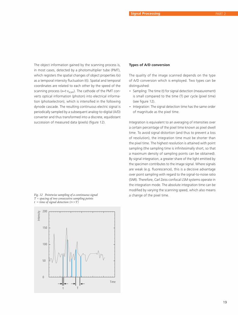
The object information gained by the scanning process is,

in most cases, detected by a photomultiplier tube (PMT),

which registers the spatial changes of object properties I(x)

as a temporal intensity fluctuation I(t). Spatial and temporal

coordinates are related to each other by the speed of the

scanning process (x=t·vscan). The cathode of the PMT con-

verts optical information (photon) into electrical informa-

tion (photoelectron), which is intensified in the following

dynode cascade. The resulting continuous electric signal is

periodically sampled by a subsequent analog-to-digital (A/D)

converter and thus transformed into a discrete, equidistant

succession of measured data (pixels) (figure 12).

19

Types�of�A/D�conversion

The quality of the image scanned depends on the type

of A/D conversion which is employed. Two types can be

distinguished:

• Sampling: The time (t) for signal detection (measurement)

is small compared to the time (T) per cycle (pixel time)

(see figure 12).

• Integration: The signal detection time has the same order

of magnitude as the pixel time.

Integration is equivalent to an averaging of intensities over

a certain percentage of the pixel time known as pixel dwell

time. To avoid signal distortion (and thus to prevent a loss

of resolution), the integration time must be shorter than

the pixel time. The highest resolution is attained with point

sampling (the sampling time is infinitesimally short, so that

a maximum density of sampling points can be obtained).

By signal integration, a greater share of the light emitted by

the specimen contributes to the image signal. Where signals

are weak (e.g. fluorescence), this is a decisive advantage

over point sampling with regard to the signal-to-noise ratio

(SNR). Therefore, Carl Zeiss confocal LSM systems operate in

the integration mode. The absolute integration time can be

modified by varying the scanning speed, which also means

a change of the pixel time.Fig. 12 Pointwise sampling of a continuous signal T = spacing of two consecutive sampling points t = time of signal detection (t<<T)

t T

Time

Inte

nsity 200

150

100

50

0

PART 2Signal�Processing

20

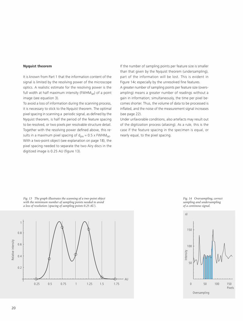
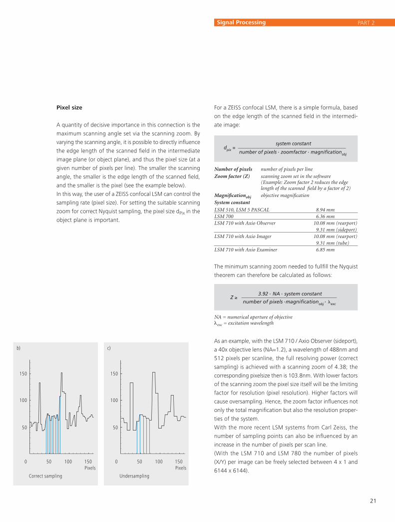
If the number of sampling points per feature size is smaller

than that given by the Nyquist theorem (undersampling),

part of the information will be lost. This is evident in

Figure 14c especially by the unresolved fine features.

A greater number of sampling points per feature size (overs-

ampling) means a greater number of readings without a

gain in information; simultaneously, the time per pixel be-

comes shorter. Thus, the volume of data to be processed is

inflated, and the noise of the measurement signal increases

(see page 22).

Under unfavorable conditions, also artefacts may result out

of the digitization process (aliasing). As a rule, this is the

case if the feature spacing in the specimen is equal, or

nearly equal, to the pixel spacing.

Fig. 13 The graph illustrates the scanning of a two-point object with the minimum number of sampling points needed to avoid a loss of resolution (spacing of sampling points 0.25 AU).

Fig. 14 Oversampling, correct sampling and undersampling of a continous signal.

Nyquist�theorem

It is known from Part 1 that the information content of the

signal is limited by the resolving power of the microscope

optics. A realistic estimate for the resolving power is the

full width at half maximum intensity (FWHMlat) of a point

image (see equation 3).

To avoid a loss of information during the scanning process,

it is necessary to stick to the Nyquist theorem. The optimal

pixel spacing in scanning a periodic signal, as defined by the

Nyquist theorem, is half the period of the feature spacing

to be resolved, or two pixels per resolvable structure detail.

Together with the resolving power defined above, this re-

sults in a maximum pixel spacing of dpix = 0.5 x FWHMlat.

With a two-point object (see explanation on page 18), the

pixel spacing needed to separate the two Airy discs in the

digitized image is 0.25 AU (figure 13).

Rela

tive

inte

nsity

1

0.8

0.6

0.4

0.2

0.25 0.5 0.75 1 1.25 1.5 1.75

AU

Inte

nsity

0 50 100 150

Oversampling

Pixels

a)

150

100

50

Pixel�size

A quantity of decisive importance in this connection is the

maximum scanning angle set via the scanning zoom. By

varying the scanning angle, it is possible to directly influence

the edge length of the scanned field in the intermediate

image plane (or object plane), and thus the pixel size (at a

given number of pixels per line). The smaller the scanning

angle, the smaller is the edge length of the scanned field,

and the smaller is the pixel (see the example below).

In this way, the user of a ZEISS confocal LSM can control the

sampling rate (pixel size). For setting the suitable scanning

zoom for correct Nyquist sampling, the pixel size dPix in the

object plane is important.

21

For a ZEISS confocal LSM, there is a simple formula, based

on the edge length of the scanned field in the intermedi-

ate image:

As an example, with the LSM 710 / Axio Observer (sideport),

a 40x objective lens (NA=1.2), a wavelength of 488nm and

512 pixels per scanline, the full resolving power (correct

sampling) is achieved with a scanning zoom of 4.38; the

corresponding pixelsize then is 103.8nm. With lower factors

of the scanning zoom the pixel size itself will be the limiting

factor for resolution (pixel resolution). Higher factors will

cause oversampling. Hence, the zoom factor influences not

only the total magnification but also the resolution proper-

ties of the system.

With the more recent LSM systems from Carl Zeiss, the

number of sampling points can also be influenced by an

increase in the number of pixels per scan line.

(With the LSM 710 and LSM 780 the number of pixels

(X/Y) per image can be freely selected between 4 x 1 and

6144 x 6144).

Number of pixels number of pixels per line

Zoom factor (Z) scanning zoom set in the software (Example: Zoom factor 2 reduces the edge length of the scanned field by a factor of 2)

Magnificationobj objective magnification

System constant

LSM 510, LSM 5 PASCAL 8.94 mm LSM 700 6.36 mm LSM 710 with Axio Observer 10.08 mm (rearport)

9.31 mm (sideport)LSM 710 with Axio Imager 10.08 mm (rearport)

9.31 mm (tube)LSM 710 with Axio Examiner 6.85 mm

0 50 100 150

Correct sampling

Pixels

b)

0 50 100 150

Undersampling

Pixels

c)

seite 15

0.88 . �em

n- n2-NA2+ 2 . n . PH

NA

2 2 0.64 . �

(n- n2-NA2)

0.64 . �

(n- n2-NA2)

0.88 . �exc

(n- n2-NA2)

n . �em

NA2

1.77 . n . �em

NA2

0.51 . �em

NA

1.77 . n . �exc

NA2

1.28 . n . �NA2

0,37 . �NA

0.51 . �exc

NA

seite 19

system constant


dpix =



Z ≥

The minimum scanning zoom needed to fullfill the Nyquist

theorem can therefore be calculated as follows:

NA = numerical aperture of objectiveλexc = excitation wavelength

seite 15

0.88 . �em

n- n2-NA2+ 2 . n . PH

NA

2 2 0.64 . �

(n- n2-NA2)

0.64 . �

(n- n2-NA2)

0.88 . �exc

(n- n2-NA2)

n . �em

NA2

1.77 . n . �em

NA2

0.51 . �em

NA

1.77 . n . �exc

NA2

1.28 . n . �NA2

0,37 . �NA

0.51 . �exc

NA

seite 19

system constant


dpix =



Z ≥

150

100

50

150

100

50


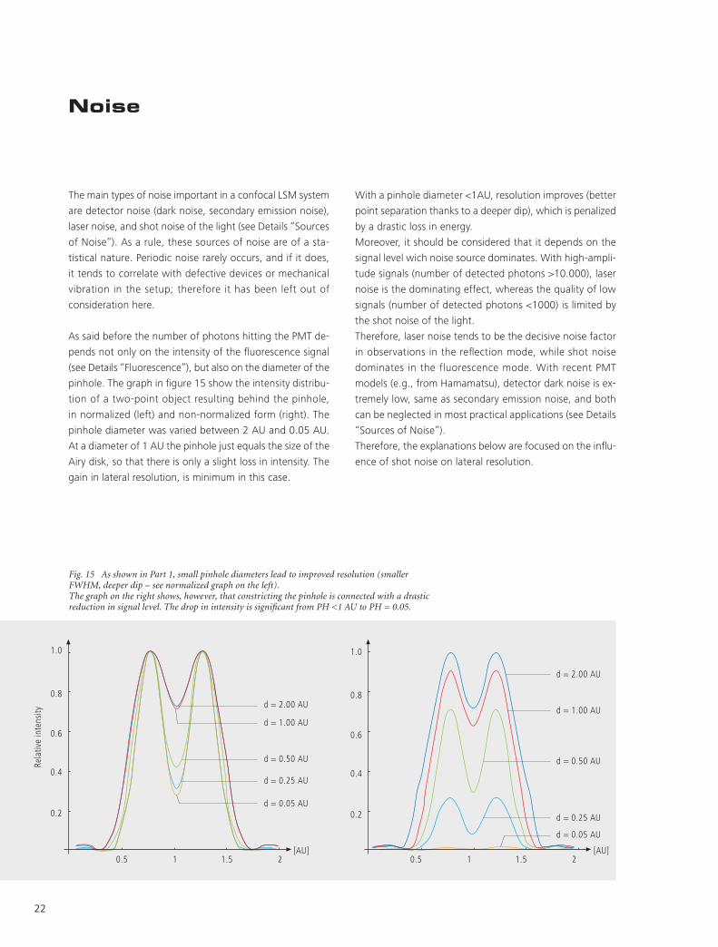
With a pinhole diameter <1AU, resolution improves (better

point separation thanks to a deeper dip), which is penalized

by a drastic loss in energy.

Moreover, it should be considered that it depends on the

signal level wich noise source dominates. With high-ampli-

tude signals (number of detected photons >10.000), laser

noise is the dominating effect, whereas the quality of low

signals (number of detected photons <1000) is limited by

the shot noise of the light.

Therefore, laser noise tends to be the decisive noise factor

in observations in the reflection mode, while shot noise

dominates in the fluorescence mode. With recent PMT

models (e.g., from Hamamatsu), detector dark noise is ex-

tremely low, same as secondary emission noise, and both

can be neglected in most practical applications (see Details

“Sources of Noise”).

Therefore, the explanations below are focused on the influ-

ence of shot noise on lateral resolution.

22

The main types of noise important in a confocal LSM system

are detector noise (dark noise, secondary emission noise),

laser noise, and shot noise of the light (see Details “Sources

of Noise”). As a rule, these sources of noise are of a sta-

tistical nature. Periodic noise rarely occurs, and if it does,

it tends to correlate with defective devices or mechanical

vibration in the setup; therefore it has been left out of

consideration here.

As said before the number of photons hitting the PMT de-

pends not only on the intensity of the fluorescence signal

(see Details “Fluorescence”), but also on the diameter of the

pinhole. The graph in figure 15 show the intensity distribu-

tion of a two-point object resulting behind the pinhole,

in normalized (left) and non-normalized form (right). The

pinhole diameter was varied between 2 AU and 0.05 AU.

At a diameter of 1 AU the pinhole just equals the size of the

Airy disk, so that there is only a slight loss in intensity. The

gain in lateral resolution, is minimum in this case.

Noise

1.0

0.8

0.6

0.4

0.2

0.5 1 1.5 2

d = 2.00 AU

d = 1.00 AU

d = 0.50 AU

d = 0.25 AU

d = 0.05 AU

[AU]

1.0

0.8

0.6

0.4

0.2

0.5 1 1.5 2

d = 2.00 AU

d = 1.00 AU

d = 0.50 AU

d = 0.25 AU

d = 0.05 AU

[AU]

Rela

tive

inte

nsity

Fig. 15 As shown in Part 1, small pinhole diameters lead to improved resolution (smaller FWHM, deeper dip – see normalized graph on the left). The graph on the right shows, however, that constricting the pinhole is connected with a drastic reduction in signal level. The drop in intensity is significant from PH <1 AU to PH = 0.05.

Resolution�and�shot�noise�–�

resolution�probability

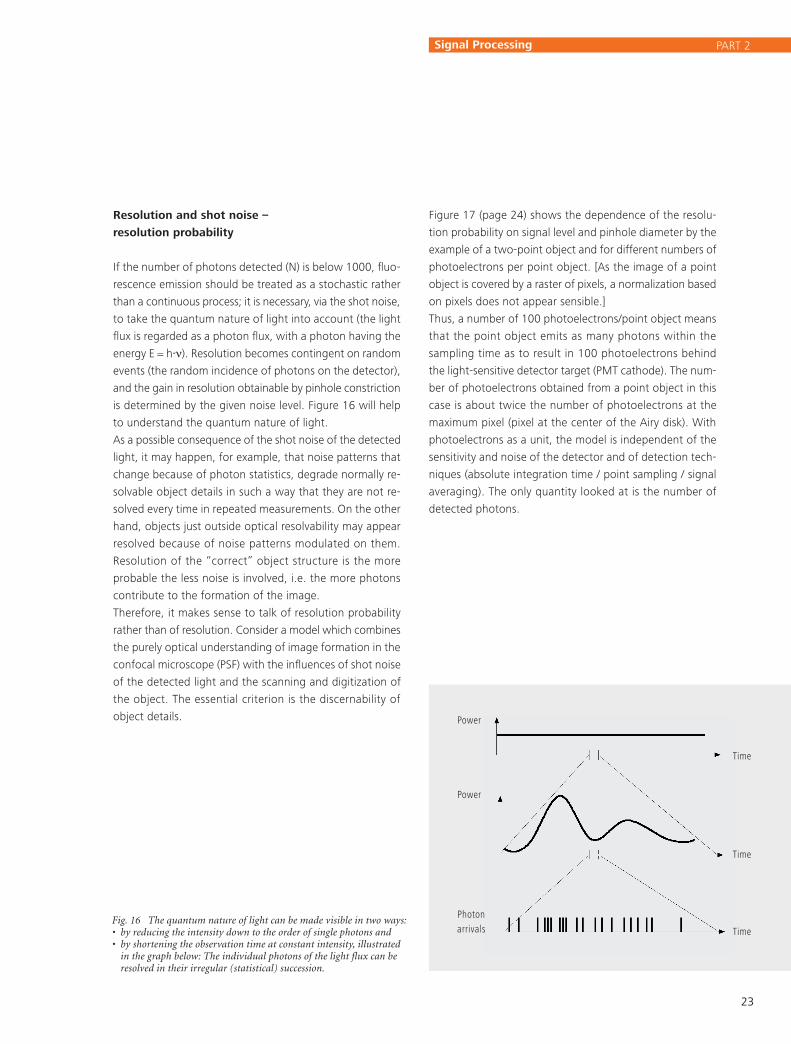
If the number of photons detected (N) is below 1000, fluo-

rescence emission should be treated as a stochastic rather

than a continuous process; it is necessary, via the shot noise,

to take the quantum nature of light into account (the light

flux is regarded as a photon flux, with a photon having the

energy E = h⋅ν). Resolution becomes contingent on random

events (the random incidence of photons on the detector),

and the gain in resolution obtainable by pinhole constriction

is determined by the given noise level. Figure 16 will help

to understand the quantum nature of light.

As a possible consequence of the shot noise of the detected

light, it may happen, for example, that noise patterns that

change because of photon statistics, degrade normally re-

solvable object details in such a way that they are not re-

solved every time in repeated measurements. On the other

hand, objects just outside optical resolvability may appear

resolved because of noise patterns modulated on them.

Resolution of the “correct” object structure is the more

probable the less noise is involved, i.e. the more photons

contribute to the formation of the image.

Therefore, it makes sense to talk of resolution probability

rather than of resolution. Consider a model which combines

the purely optical understanding of image formation in the

confocal microscope (PSF) with the influences of shot noise

of the detected light and the scanning and digitization of

the object. The essential criterion is the discernability of

object details.

23

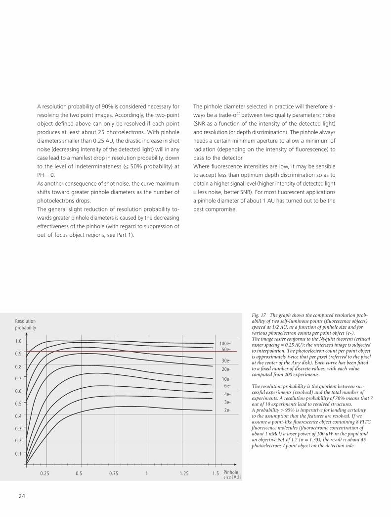
Figure 17 (page 24) shows the dependence of the resolu-

tion probability on signal level and pinhole diameter by the

example of a two-point object and for different numbers of

photoelectrons per point object. [As the image of a point

object is covered by a raster of pixels, a normalization based

on pixels does not appear sen sible.]

Thus, a number of 100 photoelectrons/point object means

that the point object emits as many photons within the

sampling time as to result in 100 photoelectrons behind

the light-sensitive detector target (PMT cathode). The num-

ber of photoelectrons obtained from a point object in this

case is about twice the number of photoelectrons at the

maximum pixel (pixel at the center of the Airy disk). With

photoelectrons as a unit, the model is independent of the

sensitivity and noise of the detector and of detection tech-

niques (absolute integration time / point sampling / signal

averaging). The only quantity looked at is the number of

detected photons.

Fig. 16 The quantum nature of light can be made visible in two ways:• by reducing the intensity down to the order of single photons and• by shortening the observation time at constant intensity, illustrated

in the graph below: The individual photons of the light flux can be resolved in their irregular (statistical) succession.

Power

Power

Photonarrivals

Time

Time

Time


The pinhole diameter selected in practice will therefore al-

ways be a trade-off between two quality parameters: noise

(SNR as a function of the intensity of the detected light)

and resolution (or depth discrimination). The pinhole always

needs a certain minimum aperture to allow a minimum of

radiation (depending on the intensity of fluorescence) to

pass to the detector.

Where fluorescence intensities are low, it may be sensible

to accept less than optimum depth discrimination so as to

obtain a higher signal level (higher intensity of detected light

= less noise, better SNR). For most fluorescent applications

a pinhole diameter of about 1 AU has turned out to be the

best compromise.

24

Fig. 17 The graph shows the computed resolution prob-ability of two self-luminous points (fluorescence objects) spaced at 1/2 AU, as a function of pinhole size and for various photoelectron counts per point object (e-).The image raster conforms to the Nyquist theorem (critical raster spacing = 0.25 AU); the rasterized image is subjected to interpolation. The photoelectron count per point object is approximately twice that per pixel (referred to the pixel at the center of the Airy disk). Each curve has been fitted to a fixed number of discrete values, with each value computed from 200 experiments.

The resolution probability is the quotient between suc-cessful experiments (resolved) and the total number of experiments. A resolution probability of 70% means that 7 out of 10 experiments lead to resolved structures.A probability > 90% is imperative for lending certainty to the assumption that the features are resolved. If we assume a point-like fluorescence object containing 8 FITC fluorescence molecules (fluorochrome concentration of about 1 nMol) a laser power of 100 µW in the pupil and an objective NA of 1.2 (n = 1.33), the result is about 45 photoelectrons / point object on the detection side.

A resolution probability of 90% is considered ne cessary for

resolving the two point images. Accordingly, the two-point

object defined above can only be resolved if each point

produces at least about 25 photoelectrons. With pinhole

diameters smaller than 0.25 AU, the drastic increase in shot

noise (decreasing intensity of the detected light) will in any

case lead to a manifest drop in resolution probability, down

to the level of indeterminateness (≤ 50% probability) at

PH = 0.

As another consequence of shot noise, the curve maximum

shifts toward greater pinhole diameters as the number of

photoelectrons drops.

The general slight reduction of resolution probability to-

wards greater pinhole diameters is caused by the decreasing

effectiveness of the pinhole (with regard to suppression of

out-of-focus object regions, see Part 1).

1.0

0.9

0.8

0.7

0.6

0.5

0.4

0.3

0.2

0.1

100e-50e-

30e-

20e-

10e-6e-

4e-

3e-

2e-

Pinholesize [AU]

Resolutionprobability

0.25 0.5 0.75 1 1.25 1.5

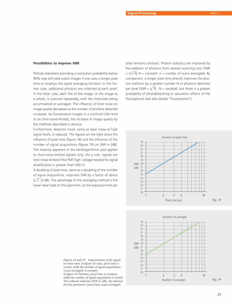
Possibilities�to�improve�SNR

Pinhole diameters providing a resolution probability below

90% may still yield useful images if one uses a longer pixel

time or employs the signal averaging function. In the for-

mer case, additional photons are collected at each pixel;

in the latter case, each line of the image, or the image as

a whole, is scanned repeatedly, with the intensities being

accumulated or averaged. The influence of shot noise on

image quality decreases as the number of photons detected

increases. As fluorescence images in a confocal LSM tend

to be shot-noise-limited, the increase in image quality by

the methods described is obvious.

Furthermore, detector noise, same as laser noise at high

signal levels, is reduced. The figures on the right show the

influence of pixel time (figure 18) and the influence of the

number of signal acquisitions (figure 19) on SNR in [dB].

The linearity apparent in the semilogarithmic plot applies

to shot-noise-limited signals only. (As a rule, signals are

shot-noise-limited if the PMT high vol tage needed for signal

amplification is greater than 500 V).

A doubling of pixel time, same as a doubling of the number

of signal acquisitions, improves SNR by a factor of about

2 (3 dB). The advantage of the averaging method is the

lower laser load on the specimen, as the exposure time per

25

pixel remains constant. Photon statistics are improved by

the addition of photons from several scanning runs (SNR

= n·N; N = constant, n = number of scans averaged). By

comparison, a longer pixel time directly improves the pho-

ton statistics by a greater number N of photons detected

per pixel (SNR = N , N = variable), but there is a greater

probability of photobleaching or saturation effects of the

fluorophores (see also details “Fluorescence”).

Figures 18 and 19 Improvement of the signal-to-noise ratio. In figure 18 (top), pixel time is varied, while the number of signal acquisitions (scans averaged) is constant. In figure 19 (bottom), pixel time is constant, while the number of signal acquisitions is varied. The ordinate indicates SNR in [dB], the abscissa the free parameter (pixel time, scans averaged).

343332313029282726252423222120

1 10

Variation of pixel time

Pixel time [�s]

SNR[dB]

2 3 4

343332313029282726252423222120

1 10

Variation of averages

Number of averages

SNR[dB]

2 3 4


Pixel time [µs] Fig. 18

SNR[dB]

343332313029282726252423222120

343332313029282726252423222120

1 10


Pixel time [�s]

SNR[dB]

2 3 4

343332313029282726252423222120

1 10


Number of averages

SNR[dB]

2 3 4


Number of averages Fig. 19

SNR[dB]

343332313029282726252423222120


The pictures on the left demonstrate the influence of pixel

time and averaging on SNR; object details can be made

out much better if the pixel time increases or averaging is

employed.

Another sizeable factor influencing the SNR of an image

is the efficiency of the detection beam path. This can be

directly influenced by the user through the selection of ap-

propriate filters and dichroic beamsplitters. The SNR of a

FITC fluorescence image, for example, can be improved

by a factor of about 2 (6dB) if the element separating the

excitation and emission beam paths is not a neutral 80/20

beamsplitter1 but a dichroic beamsplitter optimized for the

particular fluorescence.

The difficult problem of quantifying the interaction between

resolution and noise in a confocal LSM is solved by way of

the concept of resolution proba bility; i.e. the unrestricted

validity of the findings described in Part 1 is always de-

pendent on a sufficient number of photons reaching the

detector.

Therefore, most applications of confocal fluorescence mi-

croscopy tend to demand pinhole diameters greater than

0.25 AU; a diameter of 1 AU is a typical setting.

26

Fig. 20 Three confocal images of the same fluorescence specimen (mouse kidney section, glomeruli labeled with Alexa488 in green and actin labelled with Alexa 564 phalloidin in red). All images were recorded with the same parameters, except pixel time and average. The respective pixel times were 0.8 µs in a), 6.4 µs (no averaging) in b), and 6.4 µs plus 4 times line-wise averaging in c).

a)

b)

c)

1 An 80/20 beamsplitter reflects 20% of the laser light onto the specimen and transmits 80% of the emitted fluorescence to the detector.

27

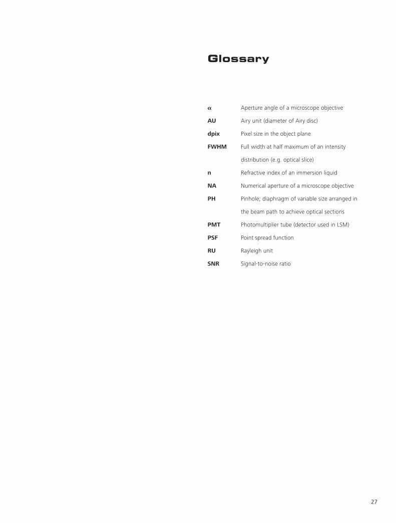
Glossary

a Aperture angle of a microscope objective

AU Airy unit (diameter of Airy disc)

dpix Pixel size in the object plane

FWHM Full width at half maximum of an intensity

distribution (e.g. optical slice)

n Refractive index of an immersion liquid

NA Numerical aperture of a microscope objective

PH Pinhole; diaphragm of variable size arranged in

the beam path to achieve optical sections

PMT Photomultiplier tube (detector used in LSM)

PSF Point spread function

RU Rayleigh unit

SNR Signal-to-noise ratio

To give some further insight into Laser Scanning Microscopy,

the following pages treat several aspects of particular importance

for practical work with a Laser Scanning Microscope.

Pupil Illumination

Optical Coordinates

Fluorescence

Sources of Noise

PART 3Details

I

Pupil Illumination

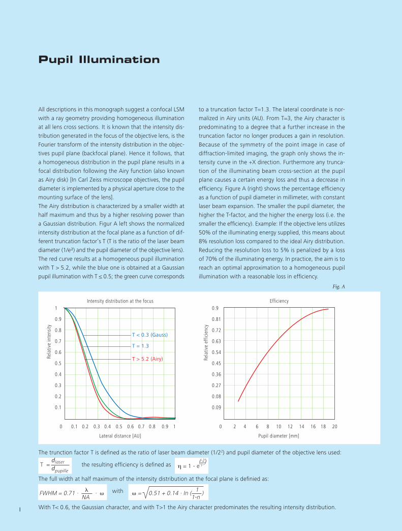
to a truncation factor T=1.3. The lateral coordinate is nor-

malized in Airy units (AU). From T=3, the Airy character is

predominating to a degree that a further increase in the

truncation factor no longer produces a gain in resolution.

Because of the symmetry of the point image in case of

diffraction-limited imaging, the graph only shows the in-

tensity curve in the +X direction. Furthermore any trunca-

tion of the illuminating beam cross-section at the pupil

plane causes a certain energy loss and thus a decrease in

efficiency. Figure A (right) shows the percentage efficiency

as a function of pupil diameter in millimeter, with constant

laser beam expansion. The smaller the pupil diameter, the

higher the T-factor, and the higher the energy loss (i.e. the

smaller the efficiency). Example: If the objective lens utilizes

50% of the illuminating energy supplied, this means about

8% resolution loss compared to the ideal Airy distribution.

Reducing the resolution loss to 5% is penalized by a loss

of 70% of the illumina ting energy. In practice, the aim is to

reach an optimal approximation to a homogeneous pupil

illumination with a reasonable loss in efficiency.

All descriptions in this monograph suggest a confocal LSM

with a ray geometry providing homogeneous illumination

at all lens cross sections. It is known that the intensity dis-

tribution generated in the focus of the objective lens, is the

Fourier transform of the intensity distribution in the objec-

tives pupil plane (backfocal plane). Hence it follows, that

a homogeneous distribution in the pupil plane results in a

focal distribution following the Airy function (also known

as Airy disk) [In Carl Zeiss microscope objectives, the pupil

diameter is implemented by a physical aperture close to the

mounting surface of the lens].

The Airy distribution is characterized by a smaller width at

half maximum and thus by a higher resolving power than

a Gaussian distribution. Figur A left shows the normalized

intensity distribution at the focal plane as a function of dif-

ferent truncation factor’s T (T is the ratio of the laser beam

diameter (1/e²) and the pupil diameter of the objective lens).

The red curve results at a homogeneous pupil illumination

with T > 5.2, while the blue one is obtained at a Gaussian

pupil illumination with T ≤ 0.5; the green curve corresponds

1

0.9

0.8

0.7

0.6

0.5

0.4

0.3

0.2

0.1

0.9

0.81

0.72

0.63

0.54

0.45

0.36

0.27

0.08

0.09

Lateral distance [AU]

T < 0.3 (Gauss)

T = 1.3

T > 5.2 (Airy)

Pupil diameter [mm]

Intensity distribution at the focus

Rela

tive

inte

nsity

Rela

tive

effic

ienc

y

Efficiency

0 0.1 0.2 0.3 0.4 0.5 0.6 0.7 0.8 0.9 1 0 2 4 6 8 10 12 14 16 18 20

Fig. A

The trunction factor T is defined as the ratio of laser beam diameter (1/22) and pupil diameter of the objective lens used:

T = the resulting efficiency is defined as The full width at half maximum of the intensity distribution at the focal plane is definied as:

with

With T< 0.6, the Gaussian character, and with T>1 the Airy character predominates the resulting intensity distribution.

dlaser

dpupille

(-2) T2h = 1 - e

FWHM = 0.71 · NA

· = 0.51 + 0.14 · In (

1-n1

)

II

Optical Coordinates

Analogously, a sensible way of normalization in the axial

direction is in terms of multiples of the wave-optical depth

of field. Proceeding from the Rayleigh criterion, the follow-

ing expression is known as Rayleigh unit (RU):

The RU is used primarily for a generally valid repre sentation

of the optical slice thickness in a confocal LSM.

In order to enable a representation of lateral and axial quan-

tities independent of the objective lens used, let us intro-

duce optical coordinates oriented to microscopic imaging.

Given the imaging conditions in a confocal microscope,

it suggests itself to express all lateral sizes as multiples

of the Airy disk diameter. Accordingly, the Airy unit (AU)

is defined as:

The AU is primarily used for normalizing the pinhole

diameter.

Thus, when converting a given pinhole diameter into AUs,

we need to consider the system’s total magnification; which

means that the Airy disk is projected onto the plane of the

pinhole (or vice versa).

n = refractive index of immersion liquidwith NA = 1.3, λ = 496 nm and n = 1.52 → 1RU = 0.446 µm

n . NA2

1AU =seite II 1.22 .

NA

1RU =

seite VSNR NPoisson = N

N =photons

QE( ) . pixel time

N = se . (N+Nd) (1+q2)

SNR = N2

se2 (N+Nd) (1+q2)SNR =

10002

1.22 (1000+100) (1+0.052)= 25.1

n . NA2


NA

1RU =


N =photons

QE( ) . pixel time

N = se . (N+Nd) (1+q2)

SNR = N2


10002

1.22 (1000+100) (1+0.052)= 25.1

PART 3Details

NA = numerical aperture of the objective λ = mean wavelength with NA = 1.3 and λ = 496 nm → 1AU = 0.465 µm

III

Fluorescence

In principle, the number of photons emitted increases with

the intensity of excitation. However, the limiting parameter

is the maximum emission rate of the fluorochrome mole-

cule, i.e. the number of photons emittable per unit of time.

The maximum emission rate is determined by the lifetime

(= radiation time) of the excited state. For fluorescein this

is about 4.4 nsec (subject to variation according to the

ambient conditions). On average, the maximum emission

rate of fluorescein is 2.27·108 photons/sec. This corresponds

to an excitation photon flux of 1.26·1024 photons/cm2 sec.

At rates greater than 1.26·1024 photons/cm2 sec, the

fluorescein molecule becomes saturated. An increase in

the excitation photon flux will then no longer cause an

increase in the emission rate; the number of photons ab-

sorbed remains constant. In our example, this case occurs

if the laser power in the pupil is increased from 500 µW

to roughly 1mW. Figure B (top) shows the relationship be-

tween the excitation photon flux and the laser power in the

pupil of the stated objective for a wavelength of 488 nm.

Figure B (bottom) illustrates the excited-state saturation of

fluorescein molecules. The number of photons absorbed

is approximately proportional to the number of photons

emitted (logarithmic scaling).

The table below lists the characteristics of some important

fluorochromes:

Source: Handbook of Biological Confocal Microscopy, p. 268/WaggonerIn the example chosen, F = 1.15·108 photons/sec or 115 photons/µsec

Fluorescence is one of the most important contrasting

methods in biological confocal microscopy.

Cellular structures can be specifically labeled with dyes

(fluorescent dyes = fluorochromes or fluorophores) in vari-

ous ways. Let the mechanisms involved in confocal fluores-

cence microscopy be explained by taking fluorescein as an

example of a fluorochrome. Fluorescein has its absorption

maximum at 490 nm. It is common to equip a confocal LSM

with an argon laser with an output of 15–20 mW at the

488 nm line. Let the system be adjusted to provide a laser

power of 500 µW in the pupil of the microscope objective.

Let us assume that the microscope objective has the ideal

transmittance of 100%.

With a C-Apochromat 63x/1.2W, the power density at the

focus, referred to the diameter of the Airy disk, then is

2.58·105 W/cm2. This corresponds to an excitation photon

flux of 6.34·1023 photons/cm2 sec. In conventional fluores-

cence microscopy, with the same objective, comparable

lighting power (xenon lamp with 2 mW at 488 nm) and a

visual field diameter of 20 mm, the excitation photon flux

is only 2.48·1018 photons/cm2 sec, i.e. lower by about five

powers of ten.

This is understandable by the fact that the laser beam in a

confocal LSM is focused into the specimen, whereas the

specimen in a conventional microscope is illuminated by

parallel light.

The point of main interest, however, is the fluorescence

(F) emitted.

The emission from a single molecule (F) depends on the

molecular cross-section (σ), the fluorescence quantum yield

(Qe) and the excitation photon flux (I) as follows:

F = σ · Qe · I [photons/sec]

Absorpt. σ/10–16 Qe σ*Q/10–16

max.(nm)

Rhodamine 554 3.25 0.78 0.91

Fluorescein 490 2.55 0.71 1.81

Texas Red 596 3.3 0.51 1.68

Cy 3.18 550 4.97 0.14 0.69

Cy 5.18 650 7.66 0.18 1.37

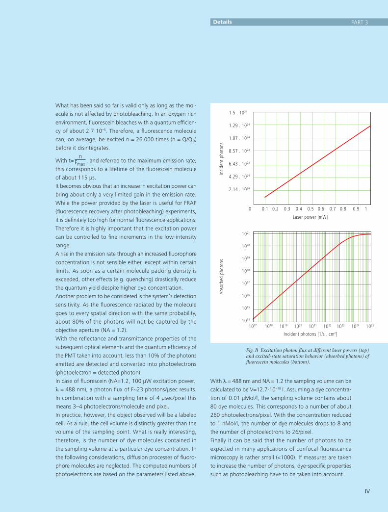
IV

With λ = 488 nm and NA = 1.2 the sampling volume can be

calculated to be V=12.7·10–18 l. Assuming a dye concentra-

tion of 0.01 µMol/l, the sampling volume contains about

80 dye molecules. This corresponds to a number of about

260 photoelectrons/pixel. With the concentration reduced

to 1 nMol/l, the number of dye molecules drops to 8 and

the number of photoelectrons to 26/pixel.

Finally it can be said that the number of photons to be

expected in many applications of confocal fluorescence

microscopy is rather small (<1000). If measures are taken

to increase the number of photons, dye-specific properties

such as photobleaching have to be taken into account.

What has been said so far is valid only as long as the mol-

ecule is not affected by photobleaching. In an oxygen-rich

environment, fluorescein bleaches with a quantum efficien-

cy of about 2.7·10–5. Therefore, a fluorescence molecule

can, on average, be excited n = 26.000 times (n = Q/Qb)

before it disintegrates.

With t= , and referred to the maximum emission rate,

this corresponds to a lifetime of the fluorescein molecule

of about 115 µs.

It becomes obvious that an increase in excitation power can

bring about only a very limited gain in the emission rate.

While the power provided by the laser is useful for FRAP

(fluorescence recovery after photobleaching) experiments,

it is definitely too high for normal fluorescence applications.

Therefore it is highly important that the excitation power

can be controlled to fine increments in the low-intensity

range.

A rise in the emission rate through an increased fluorophore

concentration is not sensible either, except within certain

limits. As soon as a certain molecule packing density is

exceeded, other effects (e.g. quenching) drastically reduce

the quantum yield despite higher dye concentration.

Another problem to be considered is the system’s detection

sensitivity. As the fluorescence radiated by the molecule

goes to every spatial direction with the same probability,

about 80% of the photons will not be captured by the

objective aperture (NA = 1.2).

With the reflectance and transmittance properties of the

subsequent optical elements and the quantum efficiency of

the PMT taken into account, less than 10% of the photons

emitted are detected and converted into photoelectrons

(photoelectron = detected photon).

In case of fluorescein (NA=1.2, 100 µW excitation power,

λ = 488 nm), a photon flux of F~23 photons/µsec results.

In combination with a sampling time of 4 µsec/pixel this

means 3–4 photoelectrons/molecule and pixel.

In practice, however, the object observed will be a labeled

cell. As a rule, the cell volume is distinctly greater than the

volume of the sampling point. What is really interesting,

therefore, is the number of dye molecules contained in

the sampling volume at a particular dye concentration. In

the following considerations, diffusion processes of fluoro-

phore molecules are neglected. The computed numbers of

photoelectrons are based on the parameters listed above.

Fmax

n

Fig. B Excitation photon flux at different laser powers (top)and excited-state saturation behavior (absorbed photons) of fluorescein molecules (bottom).

PART 3Details

1.5 . 1024

1.29 . 1024

1.07 . 1024

8.57 . 1024

6.43 . 1024

4.29 . 1024

2.14 . 1024

Laser power [mW]In

cide

nt p

hoto

ns

0 0.1 0.2 0.3 0.4 0.5 0.6 0.7 0.8 0.9 1

1021

1020

1019

1018

1017

1016

1015

1014

Incident photons [1/s . cm2]

Abso

rbed

pho

tons

1017 1018 1019 1020 1021 1022 1023 1024 1025

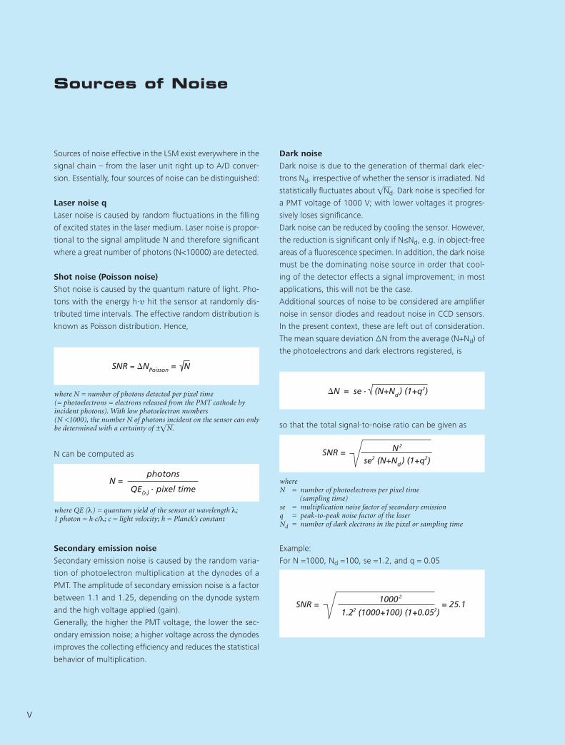
V

Sources of Noise

Dark�noise

Dark noise is due to the generation of thermal dark elec-

trons Nd, irrespective of whether the sensor is irradiated. Nd

statistically fluctuates about Nd. Dark noise is specified for

a PMT voltage of 1000 V; with lower voltages it progres-

sively loses significance.

Dark noise can be reduced by cooling the sensor. However,

the reduction is significant only if N≤Nd, e.g. in object-free

areas of a fluorescence specimen. In addition, the dark noise

must be the dominating noise source in order that cool-

ing of the detector effects a signal improvement; in most

applications, this will not be the case.

Additional sources of noise to be considered are amplifier

noise in sensor diodes and readout noise in CCD sensors.

In the present context, these are left out of consideration.

The mean square deviation ∆N from the average (N+Nd) of

the photoelectrons and dark electrons registered, is

so that the total signal-to-noise ratio can be given as

where N = number of photoelectrons per pixel time (sampling time)se = multiplication noise factor of secondary emissionq = peak-to-peak noise factor of the laserNd = number of dark electrons in the pixel or sampling time

Example:

For N =1000, Nd =100, se =1.2, and q = 0.05

Sources of noise effective in the LSM exist everywhere in the

signal chain – from the laser unit right up to A/D conver-

sion. Essentially, four sources of noise can be distinguished:

Laser�noise�q

Laser noise is caused by random fluctuations in the filling

of excited states in the laser medium. Laser noise is propor-

tional to the signal amplitude N and therefore significant

where a great number of photons (N<10000) are detected.

Shot�noise�(Poisson�noise)

Shot noise is caused by the quantum nature of light. Pho-

tons with the energy h·υ hit the sensor at randomly dis-

tributed time intervals. The effective random distribution is

known as Poisson distribution. Hence,

where N = number of photons detected per pixel time(= photoelectrons = electrons released from the PMT cathode by incident photons). With low photoelectron numbers (N <1000), the number N of photons incident on the sensor can only be determined with a certainty of ±N.

N can be computed as

where QE (λ) = quantum yield of the sensor at wavelength λ; 1 photon = h·c/λ; c = light velocity; h = Planck’s constant

Secondary�emission�noise

Secondary emission noise is caused by the random varia-

tion of photoelectron multiplication at the dynodes of a

PMT. The amplitude of secondary emission noise is a factor

between 1.1 and 1.25, depending on the dynode system

and the high voltage applied (gain).

Generally, the higher the PMT voltage, the lower the sec-

ondary emission noise; a higher voltage across the dynodes

improves the collecting efficiency and reduces the statistical

behavior of multiplication.

n . NA2


NA

1RU =


N =photons

QE( ) . pixel time

N = se . (N+Nd) (1+q2)

SNR = N2


10002

1.22 (1000+100) (1+0.052)= 25.1

n . NA2


NA

1RU =


N =photons

QE( ) . pixel time

N = se . (N+Nd) (1+q2)

SNR = N2


10002

1.22 (1000+100) (1+0.052)= 25.1

n . NA2


NA

1RU =


N =photons

QE( ) . pixel time

N = se . (N+Nd) (1+q2)

SNR = N2


10002

1.22 (1000+100) (1+0.052)= 25.1

n . NA2


NA

1RU =


N =photons

QE( ) . pixel time

N = se . (N+Nd) (1+q2)

SNR = N2


10002

1.22 (1000+100) (1+0.052)= 25.1

n . NA2


NA

1RU =


N =photons

QE( ) . pixel time

N = se . (N+Nd) (1+q2)

SNR = N2


10002

1.22 (1000+100) (1+0.052)= 25.1

Literature

1.�Beyer,�H.,�

Handbuch der Mikroskopie, 2nd Edition,

VEB Verlag Technik Berlin, (1985)

2.�Born�&�Wolf,�

Priniples of Optics,

6th edition 1988, Pergamon Press

3.�Brismar,�H.,�Trepte,�O.,�Ulfhake,�B.:�

Spectra and Fluorescence Lifetimes of Lissamine,

Rhodamine etc....: Influences of Some

Environmental Factors Recorded with a Confocal

Laser Scanning Microscope, The Journal of

Histochemistry and Cytochemistry, Vol. 43,

pp. 699-707, (7/1995)

4.�Cox,�G.,

Optical Imaging Techniques in Cell Biology,

CRC Press (2007)

5.�Keller,�H.E.,�

Objective Lens for Confocal Microscopy,

Handbook of Biological Confocal Microscopy,

pp. 111-125, Plenum Press, 2nd Edition (1995)

6.�Gröbler,�B.,�

Untersuchungen zur Bildübertragung in ab-

tastenden Mikroskopen unter besonderer

Berücksichtigung der 3D-Abbildung, PhD thesis,

University of Potsdam, (1995)

7.�Hell,�S.,�et�al.,�

Aberrations in confocal fluorescence microscopy

induced by mismatches in refractive index,

Journal of Microscopy, Vol. 169, pp. 391-405

(3/1993)

8.�Hibbs,�A.�H.,

Confocal Microscopy for Biologists, Kluwer Aca-

demic / Plenum Publishers (2004)

9.�Nitschke,�R.,Wilhelm,�S.,�et�al.,�

A modified confocal laser scanning microscope

allows fast ultraviolet ratio imaging of intracellular

Ca2+ activity using Fura 2, Euro. J. Physiologie,

Vol. 433: pp. 653-663, (1997)

10.�Oldenbourg,�R.�et�al.,�

Image sharpness and contrast transfer in coherent

confocal microscopy, Journal of Microscopy

Vol. 172, pp. 31-39, (10/1993)

11.�Pawley,�J.,�


Springer, 3rd Edition (2006)

12.�Stelzer,�E.H.K.,�

The intermediate optical system of laser scanning

confocal microscopes; Handbook of Biological

Confocal Microscopy, pp. 207-220. Springer, 3rd

Edition (2006)

13.�Stelzer,�E.H.K.,�et.�al.,�

Nondestructive sectioning of fixed and living

specimens using a confocal scanning laser

fluores cence microscope: Microtomoscopy; SPIE,

Vol. 809, pp. 130-136, (1987)

14.�Tanke,�H.J.,�van�Oostveldt,�P.,�et�al.,�

A parameter for the distribution of fluorophores

in cells derived from measurements of inner filter

effect and reabsorption phenomenon,

Cytometry Vol. 2, pp. 359-369 (6/1982)

15.�Tsien,�R.Y.,�Waggoner,�A.,�

Fluorophores for Confocal Microscopy,


pp. 338-352. Springer, 3rd Edition (2006)

16.�Webb,�R.H.,�Dorey,�C.K.,�

The Pixelated Image, Handbook of Biological Confocal

Microscopy, pp. 55-66, Plenum Press, 2nd Edition

(1995)

17.�Wilson,�T.,�Carlini,�A.R.,�

Three dimensional imaging in confocal imaging

systems with finite sized detectors; Journal of

Microscopy, Vol. 149, pp. 51-66, (1/1988)

18.�Wilson,�T.,�Carlini,�A.R.,�

Size of detector in confocal imaging systems;

Optical Letters Vol. 12, pp. 227-229, (4/1987)

19.�Wilson,�T.,�Sheppard‚�C.J.R.,�

Theory and Practice of Scanning Optical Microscopy,

Academic Press, 2nd Edition (1985)

20.�Yuste,�R.,�Konnerth,�a.,

Imaging in Neuroscience and Development,

CSHL Press (2005)

We gratefully acknowledge the assistance of Bernhard Gröbler,

Hartmut Heinz and all other staff members who contributed

to this brochure.

Carl Zeiss MicroImaging GmbH 07740 Jena, Germany

BioSciences | Jena Location Phone: +49 3641 64 3400 Telefax: +49 3641 64 3144 E-Mail: [email protected]

www.zeiss.de/lsm Info

rmat

ion

subj

ect t

o ch

ange

.Pr

inte

d on

env

ironm

enta

lly fr

iend

ly p

aper

blea

ched

wit

hout

chl

orin

e.

60-1

-003

0/e

– pr

inte

d 11

.10

ISBN

: 978

-3-9

4088

5-02

-9

Carl Zeiss Microscopy GmbH07745 Jena, [email protected]/lsm

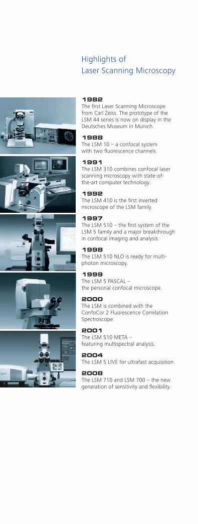
Carl Zeiss

Confocal Laser Scanning MicroscopyThis monograph comprehensively deals with the quality parameters of resolution,

depth discrimination, noise and digitization, as well as their mutual interaction.

The set of equations presented allows in-depth theoretical investigations into the

feasibility of carrying out intended experiments with a confocal LSM.

Co

nfo

cal La

ser

Sca

nn

ing

Mic

rosc

op

yC

arl Z

eiss

Highlights of Laser Scanning Microscopy

1982 The first Laser Scanning Microscope from Carl Zeiss. The prototype of the LSM 44 series is now on display in the Deutsches Museum in Munich.

1988 The LSM 10 – a confocal system with two fluorescence channels.

1991 The LSM 310 combines confocal laser scanning microscopy with state-of- the-art computer technology.

1992 The LSM 410 is the first inverted micro scope of the LSM family.

1997 The LSM 510 – the first system of the LSM 5 family and a major breakthrough in confocal imaging and analysis.

1998 The LSM 510 NLO is ready for multi - photon microscopy.

1999 The LSM 5 PASCAL – the personal confocal microscope.

2000 The LSM is combined with the ConfoCor 2 Fluorescence Correlation Spectroscope.

2001 The LSM 510 META – featuring multispectral analysis.

2004 The LSM 5 LIVE for ultrafast acquisition.

2008 The LSM 710 and LSM 700 – the new generation of sensitivity and flexibility.

Carl Zeiss


Co

nfo

cal La

ser

Sca

nn

ing

Mic

rosc

op

yC

arl Z

eiss

This monograph comprehensively

deals with the quality parameters

of resolution, depth discrimination,

noise and digitization, as well as

their mutual interaction.

The set of equations presented

allows in-depth theoretical

investigations into the feasibility of

carrying out intended experiments

with a confocal LSM.

confocal laser scanning microscopy - hcbiconfocal laser scanning microscopy confocal laser scanning...

Documents