LIBRARY RESEARCH REPORTS DIVISION NAVAL POSTGRADUATE SCHOOL

NSWC TR 83-205 MONTEREY. CAUFORNIA 93943

ff-lXIr ifl fr<

CONFIDENCE INTERVALS FOR CEP WHEN THE ERRORS ARE ELLIPTICAL NORMAL

BY AUDREY E. TAUB MARLIN A. THOMAS

STRATEGIC SYSTEMS DEPARTMENT

NOVEMBER 1983

Approved for public release; distribution unlimited.

NAVAL SURFACE WEAPONS CENTER Dahlgren, Virginia 22448 • Silver Spring, Maryland 20910

UWCLASSiFlED

'JECU.'-.ITY CLASSIFICATION QF THIS PAGE fWh«n Data Entered)

REPORT DOCUMENTATION PAGE 1. REPORT NUMBER NSWC TR 83-205

2. GOVT ACCESSION NO.

4. TITLE rand S(jbf/((9;

CONFIDENCE INTERVALS FOR CEP WHEN THE ERRORS ARE ELLIPTICAL NORMAL

7, AUTHORCJ;

Audrey E. Taub Marlin A. Thomas

3- PERFORMING ORGANIZATION NAME AND AOORESS

Naval Surface Weapons Center Code K106 Dahlgren, Virginia 22448

11. CONTROLLING OFFICE NAME AND ADDRESS

Strategic Systems Project Office Washington, D.C. 20376

U. MONITORING AGENCY NAME 4 ADDRESS^// d///er«n( Iron, Controlling Offlco)

READ INSTRUCTIONS BEFORE COMPLETING FORM

3. RECIPIENT'S CATALOG NUMBER

5. TYPE OF REPORT 4 PERIOD COVERED

Final

S. PERFORMING ORG. REPORT NUMBER

8. CONTRACT OR GRANT NUMSERrsj

10. PROGRAM ELEMENT. PROJECT TASK AREA 4 WORK UNIT NUMBERS

63371N B0951-SB

12. REPORT DATE

November 1983 13. NUMBER OF PAGES

44 IS. SECURITY CLASS, (ol Ihia report)

UNCLASSIFIED

15«. DECLASSIFl CATION/ DOWNGRADING SCHEDULE

16. DISTRIBUTION ST ATEMEN T fo/ (hi 3 ReporlJ

Approved for public release; distribution unlimited

17. DISTRIBUTION STATEMENT (ol the abmtract entered In Block 20, It dllterent Irom Report)

18. SUPPLEMENTARY NOTES

19. KEY WORDS (Continue on reverse aide II neceeetay and Identity by block number)

CEP Estimators CEP Approximations CEP Confidence Intervals Elliptical Normal Errors

20. ABSTRACT (Continue on reverse tide It neceaeary and identity by block number)

Approximate confidence intervals are developed for CEP when the delivery errors are elliptical normal. Their accuracies are determined through Monte Carlo sampling. The procedures for confidence interval computation are illu- strated via numerical examples.-

DD 1 JAN 73 1473 EDITION OF 1 NOV 65 IS OBSOLETE UNCLASSIFIED S/N 01 02-LF-OI 4-6601

SECURITY CLASSIFICATION OF THIS PAGE (When Data Bnlarad)

UNCLASSIFIED SECURITY CLASSIFICATION OF THIS PACE (Wtan Datm Enfred)

UNCLASSIFIED SECURITY CLASSIFICATION OF THIS PAGErWiM Data Bnlarad)

NSWC TR 83-205

FOREWORD

The work documented in this technical report was performed at the Naval Surface Weapons Center (NSWC) by the Mathematical Statistics Staff (K106), Space and Surface Systems Division, Strategic Systems Department. The date of com- pletion was October 1983.

This report was reviewed by Carlton W. Duke, Jr., Head, Space and Surface Systems Division.

^. Approved by:

THOMAS A. CLARE, Head Strategic Systems Department

111

NSWC TR 83-205

CONTENTS

Chapter Page

1 INTRODUCTION 1-1

2 REVIEW OF CIRCULAR CASE 2-1

3 CEP DERIVATION AND APPROXIMATIONS FOR ELLIPTICAL ERRORS ... 3-1

4 APPROXIMATE DISTRIBUTIONS OF CEP ESTIMATORS 4-1

5 APPROXIMATE CEP CONFIDENCE INTERVALS 5-1

6 MONTE CARLO VERIFICATION 6-1

BIBLIOGRAPHY 7-1

Appendix Page

A TABLE OF r(n) AND r(n + ^-j) FOR n = 1, ...,100 A-1 B TABLES OF X AND H(x) FOR x = . 1 TO 400 B-1 C THE CHI DISTRIBUTION C-1

DISTRIBUTION (1)

ILLUSTRATIONS

Figure Page

3-1 CEPi APPROXIMATION VERSUS TRUE CEP 3-3 3-2 CEPg APPROXIMATION VERSUS TRUE CEP 3-3 3-3 CEPs APPROXIMATION VERSUS TRUE CEP 3-4 3-4 CEP4 APPROXIMATION VERSUS TRUE CEP 3-4 3-5 CEP5 APPROXIMATION VERSUS TRUE CEP 3-5

NSWC TR 83-205

TABLES

Table Page

2-1 10 HYPOTHETICAL MISS DISTANCES (FEET) 2-3 5-1 12 HYPOTHETICAL MISS DISTANCES (FEET) 5-1

5-2 MULTIPLYING FACTORS OF I ^ ^ ^ j FOR CEP3 APPROXIMATION ... 5-2

6-1 SIMULATED CONFIDENCE LEVELS . . ..... 6-3 6-2 AVERAGE CONFIDENCE INTERVAL LENGTHS 6-4

VI

NSWC TR 83-205

CHAPTER 1

INTRODUCTION

A common parameter for describing the accuracy of a weapon is the circular probable error, generally referred to as CEP. CEP is simply the bivariate analog of the univariate probable error and measures the radius of a mean-centered circle which includes 50% of the bivariate probability. In the case of circular normal errors where the error variances are the same in both directions, CEP can be expressed as a function of the common miss distance standard deviation. Also, CEP estimators based on observed miss distances are easily formulated and can be used to construct confidence intervals for CEP. In the case of elliptical normal errors, CEP cannot be expressed explicitly as a function of the miss distance standard deviations. Here, one must obtain CEP by numerical methods or by re- ferring to tabular values. This has led to the development of a number of approximations by which CEP can be expressed as a function of the miss distance standard deviations. While CEP estimators based on observed miss distances are easily formulated from these approximations, their probability distributions are too complicated to be useful for CEP confidence intervals. In this report, these probability distributions are approximated with distributions which are more practical for the formulation and application of CEP confidence intervals. Ap- proximate CEP confidence intervals are then formulated and their accuracy deter- mined through Monte Carlo sampling.

The first part of this report is tutorial in the development of CEP and discusses the commonly used approximations for the elliptical case. The develop- ment of approximate confidence intervals begins with Chapter 4.

1-1

NSWC TR 83-205

CHAPTER 2

REVIEW OF CIRCULAR CASE

In general, it will be assumed that the errors in the X and Y directions

are independent with mean zero and variances a^ and a^, respectively. Under the X y circular normal assumption, a2 = QZ = Q:2 ^^^^ ^^^ bivariate distribution of errors is given by ^

f,(x,y) = 5^ e^"' * y'y^"' , - . < X, y < » (2.1)

where the subscript c denotes circular. The distribution of the radial miss distance is derived by first obtaining the distribution of the polar variables (R, 0) where

X = R cos e

Y = R sin e.

This is found to be

gj,(r,e) = 2^^ e ^ '^"^ , 0 < r < OS, 0 < e < 2n. (2.2)

The distribution of R = (X^ + Y^)"^ is now obtained from (2.2) by using the mar- ginal rule; i.e.,

27t 2/9 2

^^^^ = / 8r(^'6)de ^^ ^' ^ ' , r > 0. (2.3)

This is the well-known Rayleigh distribution (see Lindgren (1968)) with cumulative distribution function

P(R < r) = Gjr) = 1 - e -'^^/2'7^ (2.4)

By definition, G (CEP) = .5 and the solution of (2.4) yield the frequently used expression

CEP = [-2 £n(.50)]^ a = 1.1774 a. (2.5)

2-1

NSWC TR 83-205

Consider now that a (and hence, CEP) is unknown and is estimated from n observed miss distances. These miss distances will be designated as (x.,y.),

i = 1, ..., n in the X and Y directions, respectively. Moranda (1959) has shown that the maximum likelihood estimator for a is

^ = E (^i + yi)/2n [ (2.6)

and the corresponding estimator for CEP is simply CEP = 1.1774 a. This estimator

is biased for CEP, i.e., the expectation of CEP is not equal to CEP. However, the bias is small and the unbiasing factor is cumbersome. Therefore, it will be retained in its slightly biased form.

To place confidence limits on CEP, it will be necessary to examine the

probability distribution of CEP. It is well-known under normal theory (see Mood

and Graybill (1963)) that if {W.], i = 1, . . . , n is a random sample from a normal

population with mean |J and variance o^, then I(W. - \j)^/o^ has a chi-square

distribution with n degrees of freedom. One can consider {x.], i = 1, ..., n

and {y.}, i = 1, . . . , n to be a random sample of size 2n from a normal popula-

tion with mean zero and variance o^. Therefore,

n (^1 + YI) ^ 2na2 ^ 2nCEP^ 2 .■^, a^ a^ CEP^ ^2n 1=1

(2.7)

2 where "~" designates "is distributed as" and x^ designates a chi-square proba-

bility distribution with 2n degrees of freedom. The 100 (1 - a)% confidence limits are now easily constructed using the probability statement

P-^{4,a/2<^<^2n,l-a/2}=l -" • (^.8)

In this expression, x'^ designates the lOOa percentage point for a chi-square

with u degrees of freedom. Tabular values for integral u can be found in the back of most statistics texts. A more complete table is found in Hald (1952). Manipulating the inequality in (2.8) leads to the following 100 (1 - a)% con- fidence limits for CEP:

CEP CEP

(>^2n,l-a/2/2^)'' '(^2n,./2/20'^

(2.9)

The interpretation here is that one is 100 (1 - a)% confident that the interval in (2.9) contains the population CEP. This formula is valid only for the case

where the errors are known to be circular, i.e., the case where o^ = o^ = o^. ' ' X y

2-2

NSWC TR 83-205

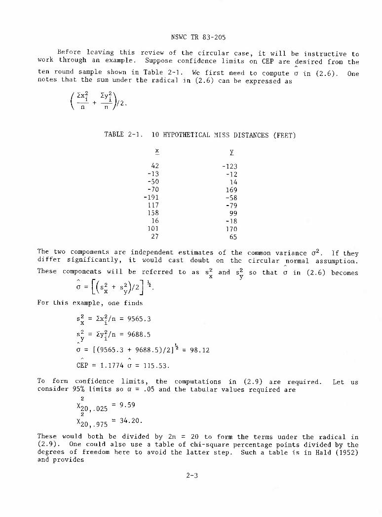
Before leaving this review of the circular case, it will be instructive to work through an example. Suppose confidence limits on CEP are desired from the

ten round sample shown in Table 2-1. We first need to compute a in (2.6). One notes that the sum under the radical in (2.6) can be expressed as

Zx2 Zy2

TABLE 2-1. 10 HYPOTHETICAL MISS DISTANCES (FEET)

42 -123 -13 -12 -50 14 -70 169

-191 -58 117 -79 158 99 16 -18

101 170 27 65

The two components are independent estimates of the common variance o^. If they differ significantly, it would cast doubt on the circular normal assumption.

These components will be referred to as s^ and s^ so that a in (2.6) becomes X y

For this example, one finds

s2 = Zx^/n = 9565.3 X 1

s^ = Zy2/n = 9688.5

a = [(9565.3 + 9688.5)/2]^' = 98.12

CEP = 1.1774 a = 115.53.

To form confidence limits, the computations in (2.9) are required. Let us consider 95% limits so a = .05 and the tabular values required are

2

^20,.025 = ^-^^ 2

^20,.975 ^ 34.20.

These would both be divided by 2n = 20 to form the terms under the radical in (2.9). One could also use a table of chi-square percentage points divided by the degrees of freedom here to avoid the latter step. Such a table is in Hald (1952) and provides

2-3

NSWC TR 83-205

^20,.025^^^ 2

X^

.4796

110 = 1.7085 '20,.975'

The 95% confidence limits on CEP can now be completed and are found to be

115.53 115.53 1, » r) = (88.39, 166.82)

(1.7085)' (.4796)'

The units are feet, the same as the miss distance units in Table 2-1. The interpretation is that one is 95% confident that the true (or population) CEP lies in the interval (88.39, 166.82). The result is valid only if the probability distribution of miss distances follows a circular normal distribution. Applica- tion of (2.9) when the probability distribution is elliptical can lead to serious errors. A discussion of the elliptical case begins with Chapter 3.

2-4

NSWC TR 83-205

CHAPTER 3

CEP DERIVATION AND APPROXIMATIONS FOR ELLIPTICAL ERRORS

In the elliptical case, the error variances are unequal and the bivariate distribution of errors is given by

1 -h[i-lo,)' + (y/a )2] » < x,y < »

x'y

where the subscript E denotes elliptical. The distribution of the radial error R for this case was derived by Chew and Boyce (1961). They proceeded, as in the circular case, by first obtaining the distribution of the polar variables (R,0). This was found to be

X y 0 < e < 27t

where

a^ + a^ a^ - a^ - y X K - y X

^ - (2a a Y ' " (2a a Y ' ^ X y/ V X y/

Using the marginal rule, the distribution of R was obtained by integrating g_(r,e) E

in (3.1) with respect to 6 between 0 and In. This integration cannot be expressed in tractable form, so they expressed their result in terms of a modified Bessel function as

2 ggCr) = —^ e ~ ^^ lo(br2), 0 < r < * . (3.2)

X y

In this expression, the subscript E denotes elliptical and IQ is a modified Bessel function of the first kind and zero order, i.e.,

-r / N _ 1 r -XCOSO j„ Io(x) = - / e de. n -'o

The cumulative distribution function for R is denoted by

P(R < r) = Gj,(r) = ^ gg(t) dt. (3.3)

3-1

NSWC TR 83-205

However, Gj,(r) cannot be expressed in tractable form because gp(t) cannot be so

expressed. This means that the radius of the 50% circle for the elliptical case cannot be expressed by a simple formula as it was in the circular case. One has to solve G„(CEP) = .5 by numerical methods or by referring to tables prepared by

Harter (1960), DiDonato and Jarnagin (1962), and others. To avoid using these tables or numerical procedures for CEP evaluation, a number of approximations have been developed over the years. Five of the most common are shown below; they are designated as CEPi through CEP5:

CEPi = 1.1774 ' ^

(j2 + (j2 \ -§

CEP2 = 1.1774 0+0 _^ y

^^P3M2xS^.5o/o^^^ g2 + (j2 \ -^

2

X V

CEP4 = .565 a + .612 o . , o . /a > .25 max min mm max ~

= .667 o + .206 o . , o . /o < .25 max min' mm max 1

CEP5 = 2Y1 - ^ 3 - - 1.

2 ^x g2 + (j2 \ 2

CEPx and CEP2 were taken from Groves (1961); CEP3 was formulated using the chi-

square approximation for calculating hit probabilities provided by Grubbs (1964). It was also derived independent of the Grubbs approximation by Thomas and Taub (1978). CEP4 is a piece-wise linear combination of standard deviations which is

commonly used in the missile community; CEP5 was formulated by Terzian (1974)

using the Wilson-Hilferty approximation for calculating hit probabilities provided by Grubbs (1964). Plots of each approximation versus the true CEP as a function of a . /o are shown in Figures 3-1 through 3-5. These give a fairly good mm max * * ^ ^ *■ indication of how well each performs. It is seen that CEP^ deteriorates rapidly

as we depart from the circular case (for which CEPi degenerates to 1.1774 a),

CEPo is reasonably good if the ratio o . la is not less than about .2; CEPQ ^ ^ * mm max ' "^

appears good for all ratios, and CEP4 and CEP5 appear good to a lesser extent

for all ratios.

3-2

NSWC TR 83-205

a- CEP, = 1.1774 j 2 ' 1

VI-

r^ LO-

i 0- § ■ ——^^ .•••• UJ

... • •

07-

.••• ...•••• C£P 1

at-

OJ- 0.0 0.1 (u aj 0.4 0.5 OJ 0 7 «J 0« 10

FIGURE 3-1. CEPj APPROXIMATION VERSUS TRUE CEP

CEP, =1.1774 1 2 J u-

^y' M-

^ ̂ «,J ^ ̂

i a.. ^i<<^

^.<^ CN

a o*- U

^ ^"

CCP 2 0.7-

0^'

..•••; .^ TRUC CEP

/^

oi) 0.1 a» 0.3 0.4 0 5 OJ 0 7 Q min/O" mo"

»M • • to

FIGURE 3-2. CEPg APPROXIMATION VERSUS TRUE CEP

3-3

NSWC TR 83-205

•J-

CEP3 = ,^ 2 , '/: (a 2 +a 2)'/^

11- y^ LO- ^^

o E ot- ^^

HI ^>^ a M^ UJ o ^ -^

ot-

■ "

CEP 3

TRUC CEP

AO ai 02 a3 a4 0.} oj a7 oa 0 m'in/O nx»

U 10

FIGURE 3-3. CEP3 APPROXIMATION VERSUS TRUE CEP

CEP^ 4 = •565a„„+.612a,,„ . ^ ^.25

"max

u- = .667 a„3, + .206a„j„ . "max v^

11- ^^

10- ^y"''^

fc 0.9- /^

D ^^ ^^

a. 04- UJ 0 ^^

0.7- -x^^*"

rrr**^"*^'^ CEP 4 r^

..TRyE_CEP_

ai-

0.0 0.1 (U 0L3 0.4 0.& 04 G min/G max

0 7 04 44 to

FIGURE 3-4. CEP4 APPROXIMATION VERSUS TRUE CEP

3-4

NSWC TR 83-205

CEP, -\}H\-^V ^ ' '

E a»-

CEP 5

TRUE CEP

0.4 0.S OJ O min/O ma*

FIGURE 3-5. CEPs APPROXIMATION VERSUS TRUE CEP

To recap the elliptical case thus far, for known values of a and a , one X y'

can compute the exact CEP by solving G (CEP) = .50 or compute an approximate CEP

by using an approximation such as CEPi to CEPQ. Consider now that a and o (and X y

hence CEP) are unknown and are to be estimated from n observed miss distances.

These miss distances will be designated as before, as (x.,y.), i = 1, ..., n in

the X and Y directions, respectively. The maximum likelihood estimators for a

and a pose no problem. They are given by

(3.4)

as shown in Lindgren (1968). These estimators are slightly biased and as before, they will not be corrected due to the cumbersome nature of the correction factor. They can now be substituted for the unknown a's in (3.3) to obtain a numerical estimate of CEP by solving G„(CEP) = .50 or they can be substituted into CEPj to

CEP5 to obtain estimates of the approximate CEP. These latter estimators will

be referred to as CEP^ to CEP5 and have the appeal of being explicitly expres-

sible. Hence, estimates of CEP for the elliptical case can be rather easily obtained.

3-5

NSWC TR 83-205

The problem of obtaining confidence limits for CEP in this case is more complex. The complexity is based on the fact that to find confidence limits for a parameter, one needs information regarding the probability distribution of the

estimator for the parameter. As previously noted, CEP can be obtained by solving

G„(CEP) = .50. Symbolically, we can write

CEP = Gg "^ (.50) (3.5)

but to obtain it requires recursive numerical integration or the use of previously noted tables. Hence, the formulation of confidence limits based on this esti- mator holds little promise for a practical solution. Therefore, we shall consider the formulation of confidence limits based on the estimators of the approximate CEP. The distributions of these estimators are extremely complicated since they involve radicals and linear combinations of sample variances and standard devi- ations. Hence, these distributions were approximated and confidence limits formulated on the basis of the approximate distributions. This development is provided in Chapter 4.

3-6

NSWC TR 83-205

CHAPTER 4

APPROXIMATE DISTRIBUTIONS OF CEP ESTIMATORS

The five estimators for CEP fall into two classes. One class involves the square root of linear combinations of sample variances and the other involves

linear combinations of sample standard deviations. CEPi, CEP3, and CEP5 fall into the first class and can be written in the form

(s2 + s2\ '"^ CEP. = K. ^% y^ , i = 1, 3, 5 (4.1)

where

Ki = 1.1774

\

K5 = [2^/^ (1 - 2/9u)] ^/^ .

CEP2 and CEP4 fall into the second class and can be written in the form

CEP. = ai s + ao s . , i = 2, 4 (4.2) 1 ^ max ^ min ' ' ^~<-'-)

where for i = 2, ai = a2 = \.\llkll

and for i = 4, ai = .565 and 32 = .612 when s . /s > .25 min max -

ai = .667 and a2 = .206 when s . /s < .25. mm max

The distribution of the square of each estimator can be approximated by a chi-square distribution with appropriate degrees of freedom. The following is the

rationale for these approximations. The squares of CEPi, CEP3, and CEP5 are

linear combinations of sample variances. Satterthwaite (1946) has shown that one can approximate the distribution of such linear combinations with a chi-square distribution with degrees of freedom chosen so the approximate distribution has a variance equal to that of the exact distribution. Here, one is approximating the distribution of a linear combination of sample variances with a chi-square. A natural extension is to approximate the distribution of a linear combination of sample standard deviations with a chi-distribution (see Appendix C). Hence,

the distributions of CEP2 and CEP4 were approximated by a chi-distribution with

degrees of freedom chosen so the approximate distribution has a variance equal

4-1

NSWC TR 83-205

to that of the exact distribution. Since the square of a chi-variable has a

chi-square distribution, the squares of CEP2 and CEP4 also have approximate chi-

square distributions. The major task is to find the appropriate degrees of free- dom for each class of estimator.

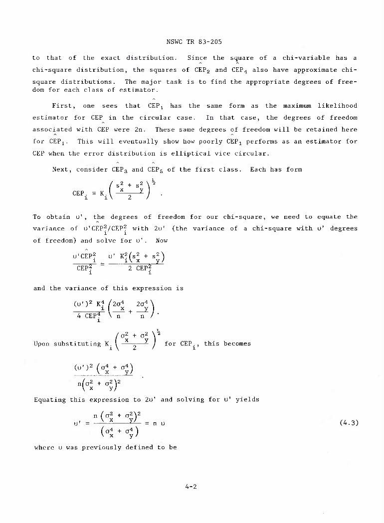
First, one sees that CEP]^ has the same form as the maximum likelihood

estimator for CEP in the circular case. In that case, the degrees of freedom

associated with CEP were 2n. These same degrees of freedom will be retained here

for CEPj. This will eventually show how poorly CEP;^ performs as an estimator for

CEP when the error distribution is elliptical vice circular.

Next, consider CEP3 and CEP5 of the first class. Each has form

g2 + s^ \ ^

CEP. = K. 1 1

To obtain u' , the degrees of freedom for our chi-square, we need to equate the

variance of u'CEP?/CEP? with 2u' (the variance of a chi-square with u' degrees

of freedom) and solve for u'. Now

U'CEP2 u' K^fs^ + s2^ 1 1 \ X V /

CEP2 2 CEP2 1

and the variance of this expression is

(u')2 K^ /2a'* 20^ \ ^[^^ + —^ . 4 CEP"* \ n n /

1

(j2 + (j2 N-^

Upon substituting K. I ^ j for CEP., this becomes

(^■)2 (^4 ^ ^4-)

V X y/

Equating this expression to 2u' and solving for u' yields

n (a^ + o^Y u- = ^ ^^ = n u (4.3)

(a4 + a*)

where U was previously defined to be

4-2

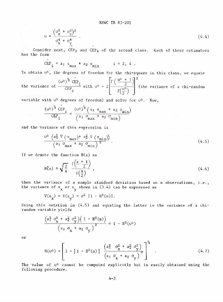
NSWC TR 83-205

a* + a^ X y

(4.4)

Consider next, CEP2 and CEP4 of the second class. Each of these estimators has the form

CEP. = ai s + ao s . i = 2, 4 . 1 max ^ min '

To obtain U", the degrees of freedom for the chi-square in this class, we equate

(0")"^ CEP. the variance of

CEP. — with U" - 2

fr ( ^" "■ - '1 ' "v 2

L r(r) (the variance of a chi-random

variable with u^'^ degrees of freedom) and solve for U". Now,

(U-^)''' CEP. (u^V)^ /ai s + 32 s . ") 1 _ V max ^ mm/

CEP. /ai a + ao cj . \ (^ max min )

and the variance of this expression is

U" faf V (^s ^+ a§ V /s . )") V V max/ ^ \ mm// /ai o + ao a . Y~^ ■ \ max min ^

If we denote the function H(x) as

^x + 1

(4.5)

Htx) = VI r

Kl) ' (4.6)

then the variance of a sample standard deviation based on n observations, i.e., the variance of s or s shown in (3.4) can be expressed as

X y ^

V(s ) = V(s ) = aMl - H2(n)]. X y

Using this notation in (4.5) and equating the latter to the variance of a chi- random variable yields

(a? o2 + ai a2)(l - H2(n))

ai a + ao X y ^ ) V /

= 1 - H2(U")

or

H(U") = 1 - |l - H2(n)[ fa? a^ + a| a^ ") V ^ X y \.

(ai a^ + ^2 a ) (4.7)

The value of U" cannot be computed explicitly but is easily obtained using the following procedure.

4-3

NSWC TR 83-205

Evaluate the right-hand side of (4.7) using estimates of a and o obtained X y

from n sample data points and values of aj and a2 determined by (4.2). Call

this value w. Refer to Appendix B which contains tabled values of x and H(x). Enter the table and find the value of x for which H(x) = w. This value of x is U". An example which incorporates this procedure begins in Chapter 5.

Clearly, u' and U" may take on fractional (non-integral) values. However, this poses no problem. Although the question of fractional degrees of freedom is rarely addressed in standard statistics texts, an extensive table of chi- square percentage points with fractional degrees of freedom has been generated by DiDonato and Hageman (1977). Also, one can obtain such percentage points using the MDCHl subroutine available in IMSL (1982).

For each of the five CEP estimators, it has been shown that the distribution of

u. CEP2

CEP'-^ i = 1, 2, ... 5 (4.8) i

can be approximated by a chi-square distribution with u. degrees of freedom where

u^ is either 2n, u' , or U" defined previously. Since the form of a confidence

interval for a chi-square random variable is well-known, construction of con- fidence intervals for CEP, using (4.8), is straightforward.

4-4

NSWC TR 83-205

CHAPTER 5

APPROXIMATE CEP CONFIDENCE INTERVALS

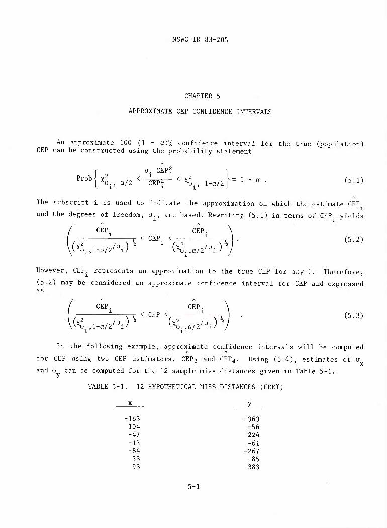
An approximate 100 (1 - oi)% confidence interval for the true (population) CEP can be constructed using the probability statement

r u. CEP2 ^

P'^^^l^^u^, a/2 < ilPf^ < ^l, l-a/2|= ^ " « " (5.1)

1 The subscript i is used to indicate the approximation on which the estimate CEP.

and the degrees of freedom, u., are based. Rewriting (5.1) in terms of CEP. yields

CEP. CEP. T < CEP. <^ TT 1 • (5.2)

X^u.,l-a/2/^)'' ' (>'u.,a/2/"i)

However, CEP represents an approximation to the true CEP for any i. Therefore,

(5.2) may be considered an approximate confidence interval for CEP and expressed as

CEP. CEP. ^ -^ < CEP < . i -p I . (5.3)

.(^u.,l-a/2/"x)'^ (x5.,a/2/"x)'^

In the following example, approximate confidence intervals will be computed

for CEP using two CEP estimators, CEP3 and CEP4. Using (3.4), estimates of a

and a can be computed for the 12 sample miss distances given in Table 5-1.

TABLE 5-1. 12 HYPOTHETICAL MISS DISTANCES (FEET)

X y

-163 -363 104 -56 -47 224 -13 -61 -84 -267 53 -85 93 383

5-1

NSWC TR 83-205

TABLE 5-1. (Cont.)

X y

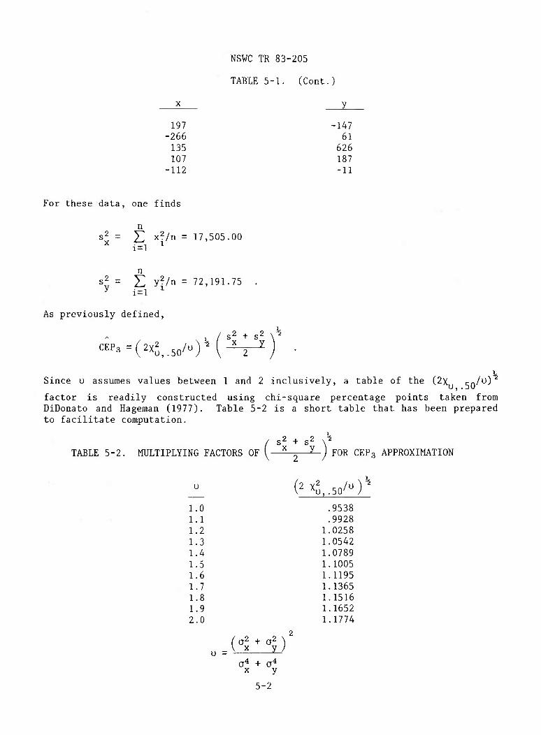
197 -147 -266 61 135 626 107 187

-112 -11

For these data, one finds

n s2 = ^ x2/n = 17,505.00 ^ i=l ^

s^ = X! y^/n = 72,191.75 .2

'y

1

, / s2 + s2 N^

i=l

As previously defined,

Since u assumes values between 1 and 2 inclusively, a table of the (2x so^^^

factor is readily constructed using chi-square percentage points taken from DiDonato and Hageman (1977). Table 5-2 is a short table that has been prepared to facilitate computation.

g2 + g2 ,^

TABLE 5-2. MULTIPLYING FACTORS OF V^—^j FOR CEP3 APPROXIMATION

^ (^^o,.50/")

1.0 .9538 1.1 .9928 1.2 1.0258 1.3 1.0542 1.4 1.0789 1.5 1.1005 1.6 1.1195 1.7 1.1365 1.8 1.1516 1.9 1.1652 2.0 1.1774

_KJL1) u = a"* + t

y

5-2

NSWC TR 83-205

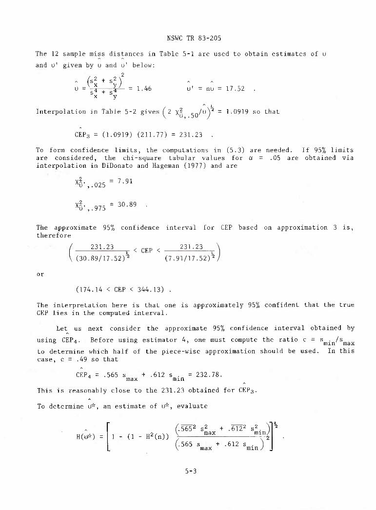
The 12 sample miss distances in Table 5-1 are used to obtain estimates of u

and u' given by u and u' below:

^s2 + s2 X yy _

s"* + s' 1.46 nu = 17.52

Interpolation in Table 5-2 gives (2 x- so^^)^ ~ 1.0919 so that

CEPs = (1.0919) (211.77) = 231.23 .

To form confidence limits, the computations in (5.3) are needed. If 95% limits are considered, the chi-square tabular values for a = .05 are obtained via interpolation in DiDonato and Hageman (1977) and are

^u' ,.025 ^ ''■^^

X^,^.975- 30.89 .

The approximate 95% confidence interval for CEP based on approximation 3 is, therefore

231.23 / .„!, ^ 231.23 i~ < CEP < r

(30.89/17.52)' (7.91/17.52)'

or

(174.14 < CEP < 344.13) .

The interpretation here is that one is approximately 95% confident that the true CEP lies in the computed interval.

Let us next consider the approximate 95% confidence interval obtained by

using CEP4. Before using estimator 4, one must compute the ratio c = s . /s

to determine which half of the piece-wise approximation should be used. In this case, c = .49 so that

CEP4 = .565 s + .612 s . = 232.78. ^ max min

This is reasonably close to the 231.23 obtained for CEP3.

To determine O", an estimate of U", evaluate

H(u>V) = 1 - (1 - H2(n)) 565 2 s2 + .6122 s2

max min

.565 s + .612 s . max min

5-3

NSWC TR 83-205

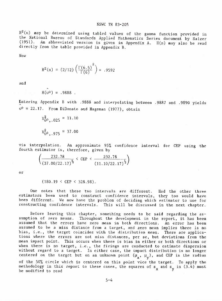
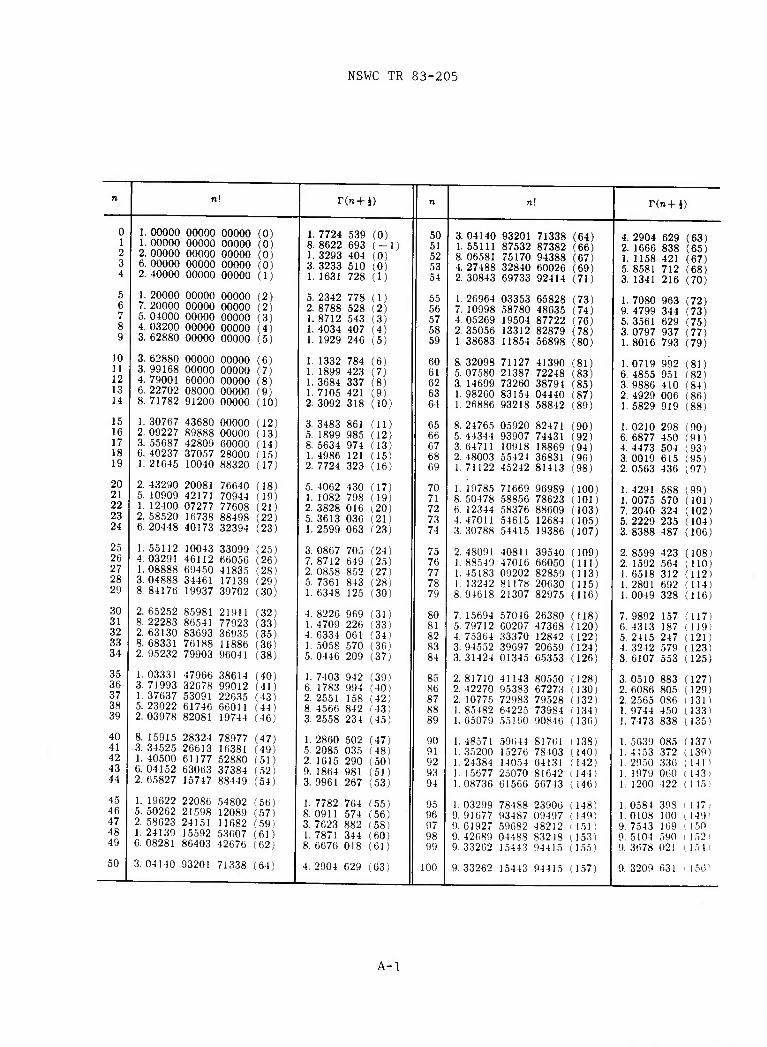
H (n) may be determined using tabled values of the gamma function provided in the National Bureau of Standards Applied Mathematics Series document by Salzer (1951). An abbreviated version is given in Appendix A. H(n) may also be read directly from the table provided in Appendix B.

Now

H2(n) = (2/12) [^J^ ) = .9592

and

H(u^V) = .9888 .

Entering Appendix B with .9888 and interpolating between .9887 and .9890 yields

U" = 22.17. From DiDonato and Hageman (1977), obtain

^G*,.975= 37.00

via interpolation. An approximate 95% confidence interval for CEP using the fourth estimator is, therefore, given by

232.78 ^ ^j,p ^ 232.78

(37.00/22.17)^ (11.10/22.17) 17)0 or

(180.19 < CEP < 328.98).

One notes that these two intervals are different. Had the other three estimators been used to construct confidence intervals, they too would have been different. We now have the problem of deciding which estimator to use for constructing confidence intervals. This will be discussed in the next chapter.

Before leaving this chapter, something needs to be said regarding the as- sumption of zero means. Throughout the development in the report, it has been assumed that the errors have zero mean in both directions. An error has been assumed to be a miss distance from a target, and zero mean implies there is no bias, i.e., the target coincides with the distribution mean. There are applica- tions where the errors are not miss distances, per se, but deviations from the mean impact point. This occurs when there is bias in either or both directions or when there is no target, i.e., the firings are conducted to estimate dispersion without regard to a target. In either case, the impact distribution is no longer centered on the target but on an unknown point (|j , |J ), and CEP is the radius

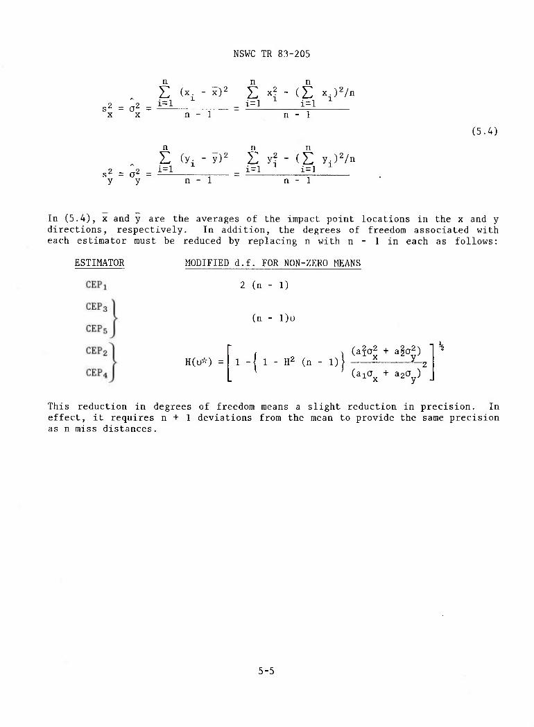
X y of the 50% circle which is centered on this point vice the target. To apply the methodology in this report to these cases, the squares of s and s in (3.4) must be modified to read ^

5-4

NSWC TR 83-205

n

s2 = a2 X X

s2 = a2

i=l n - 1

E (y. - y)= i=l

n - 1

E x2 - (E x.)2/n i=l i=l

n - 1

(5.4)

E yf - (E ypVn i=l i=l

n - 1

In (5.4), X and y are the averages of the impact point locations in the x and y directions, respectively. In addition, the degrees of freedom associated with each estimator must be reduced by replacing n with n - 1 in each as follows:

ESTIMATOR MODIFIED d.f. FOR NON-ZERO MEANS

2 (n - 1)

(n - l)u

H(U") = 1 -I 1 - H2 (n - 1)} ^ (aiQ + aoO )

^ X ^ y

This reduction in degrees of freedom means a slight reduction in precision. In effect, it requires n + 1 deviations from the mean to provide the same precision as n miss distances.

5-5

NSWC TR 83-205

CHAPTER 6

MONTE CARLO VERIFICATION

To ascertain if the formulated approximations produced confidence intervals with confidence close to 1 - a, a Monte Carlo simulation was written for the CDC 6700. This would also provide a means of comparing the estimators with respect to their confidence level and their expected confidence interval length. One replicate of the simulation entailed generating a sample of n miss distances from a bivariate normal distribution with zero mean and variances o^ and o^

X y' These n values were then used to compute a CEP confidence interval using the

five estimators CEPi to CEP5. The length of each interval was computed, and for

each interval, it was determined whether the interval contained the true (popula- tion) CEP. This process was replicated N = 10,000 times. The proportion of replicates in which the confidence interval contained the true CEP provided an estimate of the confidence associated with each estimator, and the average interval length for each provided an estimate of the expected length.

The values of the parameters used in the simulation are:

n = number of miss distances = sample size = 5, 10, 20

N = number of replicates = 10,000

1 - a = nominal confidence level = .95

' = %in/^max= ^'O' ■^^' '^O, -35, .20, .05.

It was necessary to run a large number of replicates to ensure results with reasonable precision. The 10,000 replicates used provided estimates of confidence with an error of less than .01 with probability .95. Because of the large N, the sample sizes were restricted to small values to keep the computer time within bounds. A nominal value of a = .05 ( > a nominal confidence level of .95) was used in the construction of all confidence intervals within the simula- tion. It follows that if the confidence intervals were exact (vice approximate), the Monte Carlo confidence estimates should be within .01 of .95 or .95 ± .01 with probability .95. Hence, any confidence estimate which departs seriously from .95 ± .01 will reflect poorly on the estimator which produced it. One additional comment is required before discussing the results. The simulated confidence levels depend only on the ratio of the sigmas so that it was not neces- sary to vary both standard deviations. The larger was designated a and set equal

to unity while the smaller was designated a and set equal to the ratio c. While

the average confidence interval lengths are dependent on both sigmas, they were

6-1

NSWC TR 83-205

only constructed for a^ = c, a = 1. This is all that is required for comparison

purposes. If such lengths are needed for values of a and a other than c and 1, X y '

they can be obtained by multiplying the tabled entry for appropriate c by a = a . y max

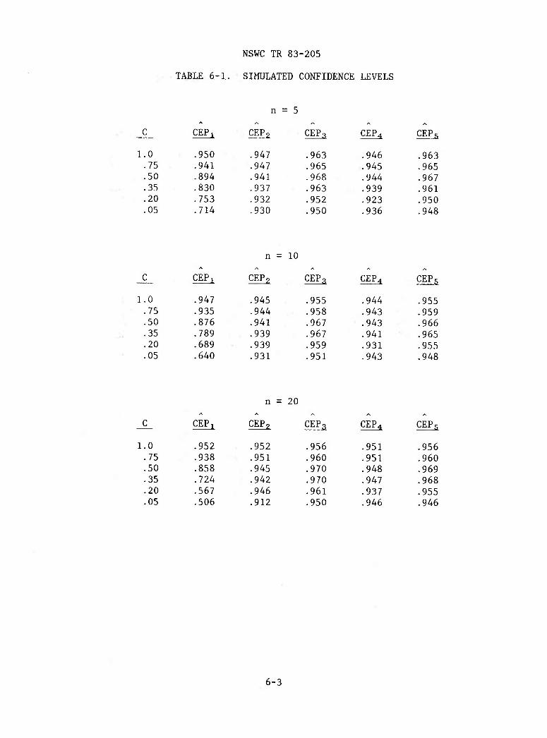
The results of the simulations are set out in Tables 6-1 and 6-2. Let us first discuss the simulated confidence levels shown in Table 6-1. One first notes that all five estimators provide confidence within (or nearly within) the sampling variations (±.01) of .95 when c = 1. This is the circular case and

all the estimators except CEP5 degenerate properly to the maximum likelihood

estimator for CEP. Hence, the result that all do well for c = 1 is not unex- pected. Next, one notes that as c departs from unity (that is, as the impact

distribution departs from circularity), the confidence associated with CEPi

departs seriously from .95. For example, with n = 10 and c = .20 (5 to 1 ratio

of the sigmas) the confidence associated with CEPi is only .689. This means that if one were to use circular theory to construct a 95% confidence interval for CEP when the distribution was elliptical with a 5 to 1 ratio of the sigmas, his

interval would have confidence of less than .7! This rules out CEPi unless one

is nearly certain that the impact distribution is circular normal. This result is also not unexpected, but it does quantify how poorly the circular estimator performs in the elliptical case.

In general, the others do reasonably well unless c is small. One notes this

especially for CEP2 when c = .05; the confidence falls from .930 for n = 5 to

.912 for n = 20. It would continue to decrease as n increases due, to the error

in CEP approximation for small c (see Figure 3-2). The distribution of CEP2 becomes more concentrated about the approximate CEP as n increases. If the approximation is in serious error (which it is for small c), then the distribution is concentrated about the wrong value. The simulation was run for n = 100 at c = .05 with a resulting confidence estimate of only .714. We see the same behavior at larger c values but to a lesser extent. For example, at c =; .35, the confidence estimate is .942 for n = 20 but dips to .922 for n = 100. The

upshot here is that CEP2 would be a problem for small c or even moderate c if

the sample is large enough. With regard to CEP3, one sees that small values of

c pose no problem. In fact, the confidence for CEP3 is asymptotic to .95 at

c = 0. Also, for values of c around .5, the confidence estimates are slightly higher than .95. It tends to peak out at about .97. Selected runs for n = 100 show that this result changes very little with n. There is a slight price to pay for this extra confidence, and this will be addressed when Table 6-2 is

discussed. CEP4 provides confidence close to .95 for all values of c except

those where CEP4 departs from CEP (see Figure 3-4). At those values, there is

a reduction in confidence which increases with n but not as severely as for

CEP2. The performance of CEP5 is not poor with respect to confidence. However,

6-2

NSWC TR 83-205

TABLE 6-1. SIMULATED CONFIDENCE LEVELS

c CEPi CEPj> CEP3 CEP4 CEP,s

1.0 .950 .947 .963 .946 .963 .75 .941 .947 .965 .945 .965 .50 .894 .941 .968 .944 .967 .35 .830 .937 .963 .939 .961 .20 .753 .932 .952 .923 .950 .05 .714 .930 .950 .936 .948

10

c CEP^ CEPj> CEP 3 CEP4 CEP,s

1.0 .947 .945 .955 .944 .955 .75 .935 .944 .958 .943 .959 .50 .876 .941 .967 .943 .966 .35 .789 .939 .967 .941 .965 .20 .689 .939 .959 .931 .955 .05 .640 .931 .951 .943 .948

20

C CEPi CEP5, CEP3 CEP4 CEPs

1.0 .952 .952 .956 .951 .956 .75 .938 .951 .960 .951 .960 .50 .858 .945 .970 .948 .969 .35 .724 .942 .970 .947 .968 .20 .567 .946 .961 .937 .955 .05 .506 .912 .950 .946 .946

6-3

NSWC TR 83-205

TABLE 6-2. AVERAGE CONFIDENCE INTERVAL LENGTHS

n = 5

CEPi CEPc CEPc CEP, CEPr

;

.0

.75

.50

.35

.20

.05

1.213 1.071 .950 .897 .856 .841

1.160 1.028 .923 .889 .876 .912

305 175 118 129 149 176

1.145 1.014

.918

.917

.985 1.054

317 186 131 144 168 196

= 10

.0

.75

.50

.35

.20

.05

CEPi

.792

.698

.622

.587

.564

.553

CEP2

.776

.685

.614

.586

.573

.579

CEPa

.817

.735

.697

.693

.694

.695

CEP^

.768

.676

.601

.586

.636

.662

CEPs

.823

.741

.705

.702

.706

.707

n = 20

1.0 .75 .50 .35 .20 .05

CEPi

.537

.475

.423

.400

.384

.378

CEP^

.533

.472

.421

.401

.388

.387

CEP.-,

.5^5

.492

.465

.460

.455

.453

CEP^

.531

.467

.411

.393

.429

.441

CEPs

.549

.496

.470

.466

.462

.461

6-4

NSWC TR 83-205

there is little rationale for its use in constructing confidence intervals. The Wilson-Hilferty approximation avoids the use of chi-square percentage points for

fractional degrees of freedom in forming CEP4. However, they are needed in the

computation of the interval, so little effort is saved.

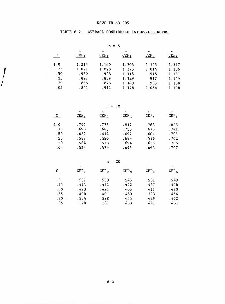
Let us now discuss the average confidence interval lengths in Table 6-2. As

previously noted, these lengths depend on both a and o but were computed only X y

for values of the ratio of a to a for comparison purposes. However, we need X y

not compare all five since some were eliminated as viable candidates in our

discussions of Table 6-1. CEPj was eliminated because its confidence eroded

seriously as c departed from unity. CEP2 had a less serious but similar problem,

and CEP5 was eliminated because it offered no improvement over CEP3 and only

a slight reduction in computation. This leaves only CEP3 and CEP4 to discuss

here. One notes that the average lengths are uniformly less for CEP4 than for

CEP3. At mid values of c, this is due in part to the inflated confidence

inherent in the approximation of the distribution of CEP3, i.e., the higher the

confidence, the longer the confidence length. However, not all of the difference in length can be attributed to higher confidence. A study by Taub and Thomas

(1982) shows that the variance of CEP4 is less than the variance of CEP3, and

this is the primary reason for the difference in length. Even so, CEP4 suffers

from the bias caused by the error in approximation shown in Figure 3-4. This has

an effect on the confidence level associated with CEP4 for some values of c, but

it would not be appreciable for small n.

In summary, we can state that the logical choice lies between CEP3 and

CEP4. The third holds for all values of c, regardless of n, and is easy to imple-

ment. The fourth offers somewhat shorter confidence lengths but it is cumbersome to implement and would provide a reduced confidence level for some values of n and c.

It would be highly desirable to have a CEP estimator with a variance as

small or smaller than CEP4 which would have negligible bias for all 0 < c < 1,

and which would avoid the cumbersomeness of a piece-wise linear function. The authors have several ideas along this line and hope to explore their merits in the near future.

6-5

NSWC TR 83-205

BIBLIOGRAPHY

Chew, Victor and Boyce, Ray, 1962, "Distribution of Radial Error in the Bivariate Elliptical Normal Distribution," Technometrics, Vol. 4, 138-140.

DiDonato, A. R. and Jarnagin, M. P., 1962, A Method for Computing the Generalized Circular Error Function and the Circular Coverage Function, NWL R^^^rt 1768" Naval Weapons Laboratory, Dahlgren, VA. '

DiDonato, A. R. and Hageman, R. K. , 1977, Computation of the Percentage Points of the Chi-Square Distribution. NSWC/DL TR-3569, Naval Surface Weapons Center Dahlgren, VA.

Groves, A. D., 1961, "Handbook on the Use of the Bivariate Normal Distribution in Describing Weapon Accuracy," BRL Memorandum Report No. 1372, Aberdeen, MD.

Grubbs, Frank E., 1964, "Approximate Circular and Non-Circular Offset Probabilities of Hitting," Operations Research, Vol. 12, No. 1.

Hald, A., 1952, Statistical Tables and Formulas, John Wiley and Sons, Inc New York, N.Y. '

Barter, H. Leon, I960, "Circular Error Probabilities," JASA, 55:723-731.

IMSL Reference Manual, MDCHI-1 1982, Volume 2, Chapter M, Edition 9, (ISML LIB-

Krutchkoff, Richard G. , 1970, Probability and Statistical Inference, Gordon and Breach Science Publishers, New York, N.Y.

Lindgren, B. W. , 1968, Statistical Theory, The MacMillan Company, New York, N.Y.

Mood, Alexander M. and Graybill, Franklin A., 1963, Introduction to the Theory of Statistics, McGraw Hill Book Company, Inc., New York, N.Y.

Moranda, P. B. , 1959, "Comparison of Estimates of Circular Probable Error," JASA 54:795-800.

Satterthwaite, F. E., 1946, "An Approximate Distribution of Estimates of Variance Components," Biometrices, Vol. 2, 110-114.

Salzer,^Herbert E., 1951, "Tables of n! and r(n + k) for the First Thousand Values of n," National Bureau of Standards Applied Mathematics Series 16, Washington DC.

7-1

NSWC TR 83-205

Terzian, R. C, 1974, Discussion of "A Note on CEP's," IEEE Transactions on Aero- space and Electronic Systems.

Taub, A. E., and Thomas, M. A., 1982, "Comparison of CEP Estimators for Elliptical Normal Errors," Proceeding of the Twenty-Eighth Conference on the Design of Ex- periments in Army Research, Development and Testing.

Thomas, M. A. and Taub, A. E., 1978, Weapon Accuracy Assessment for Elliptical Normal Miss Distances, NSWC/DL TR-3777, Naval Surface Weapons Center, Dahlgren, VA.

7-2

NSWC TR 83-205

APPENDIX A

TABLE OF r(n) AND r(n + %) FOR n = 1, ... 100

Excerpted from National Bureau of Standards

Applied Mathematics Series - 16

by

Herbert E. Salzer

NSWC TR 83-205

10 II 12 13 14

15 16 17 18 19

20 21 22 23 24

25 26 27 28 29

30 31 32 33 34

35 36 37 38 39

40 41 42 43 44

46 47 48 49

50

1. 00000 00000 00000 (0) 1. 00000 00000 00000 (0) 2. 00000 00000 00000 (0) 6. 00000 00000 00000 (0) 2. 40000 00000 00000 (1)

1. 20000 00000 00000 (2) 7. 20000 00000 00000 (2) 5. 04000 00000 00000 (3) 4. 03200 00000 00000 (4) 3. 62880 00000 00000 (5)

3. 62880 00000 00000 (6) 3. 99168 00000 00000 (7) 4. 79001 60000 00000 (8) 6. 22702 08000 00000 (9) 8. 71782 91200 00000 (10)

1. 30767 43680 00000 2. 09227 89888 00000 3. 55687 42809 60000

(12) (13)

(14) 6. 40237 37057 28000 (15) 1. 21645 10040 88320 (17)

2. 43290 20081 76640 (18) 5. 10909 42171 70944 (19) 1. 12400 07277 77608 (21) 2. 58520 16738 88498 (22) 6. 20448 40173 32394 (23)

1. 55112 10043 33099 (25) 4. 03291 46112 66056 1. 08888 69450 41835 3. 04888 34461 17139

(26) (28)

(29) 8. 84176 19937 39702 (30)

2. 65252 8. 22283 2. 63130 8. 68331 2. 95232

1. 03331 3. 71993 1. 37637 5. 23022 2. 03978

85981 86541 83693 76188 79903

47966 32678 53091 61746 82081

21911 77923 36935 11886 96041

38614 99012 22635 66011 19744

(32) (33) (35) (36) (38)

(40) (41) (43) (44) (46)

8. 15915 28324 78977 (47) (49) (51) (52)

2. 65827 15747 88449 (54)

3. 34525 26613 16381 1. 40500 61177 52880 6. 04152 63063 37384

1. 19622 22086 54802 5. 50262 21598 12089 2. 58623 24151 1. 24139 6. 08281

(56) (57)

11682 (59)

r(n+J)

15592 53607 86403 42676

(61, (62)

3. 04140 93201 71338 (64)

1. 7724 539 (0) 8. 8622 693 ( - 1) 1. 3293 404 (0) 3. 3233 510 (0) 1. 1631 728 (1)

5. 2342 778 (1) 2. 8788 528 (2) 1. 8712 543 (3) 1. 4034 407 (4) 1. 1929 246 (5)

1. 1332 784 (6) 1. 1899 423 (7) 1. 3684 337 (8) 1. 7105 421 (9) 2. 3092 318 (10)

3. 3483 861 (11) 5. 1899 985 (12) 8. 5634 974 (13) 1. 4986 121 (15) 2. 7724 323 (16)

5. 4062 430 (17) 1. 1082 798 (19) 2. 3828 016 (20) 5. 3613 036 (21) 1. 2599 063 (23)

3. 0867 705 (24) 7. 8712 649 (25) 2. 0858 852 (27) 5^ 7361 843 (28) 1. 6348 125 (30)

4. 8226 969 (31) 1. 4709 226 (33) 4. 6334 061 (34) 1. 5058 570 (36) 5. 0446 209 (37)

1. 7403 942 (39) 6. 1783 994 (40) 2. 2551 158 (42) 8. 4566 842 C43) 3. 2558 234 (45)

1. 2860 502 (47) 5. 2085 035 f48) 2. 1615 290 (50) 9. 1864 981 (51) 3. 9961 267 (53)

1. 7782 764 (55) 8, 0911 574 (56) 3. 7623 882 (58) 1. 7871 344 (60) 8. 6676 018 (61)

4. 2904 629 (63)

50 51 52 53 54

55 56 57 58 59

60 61 62 63 64

65 66 67 68 69

70 71 72 73 74

75 76 77 78 79

80 81 82 83 84

85 86 87 88 89

90 91 92 93 94

95 96 97 98 99

100

3. 04140 93201 71338 1. 55111 87532 87382 8. 06581 75170 94388 4. 27488 32840 60026 2 30843 69733 92414

1. 26964 03353 65828 7 10998 58780 48635 4. 05269 19504 87722 2 35056 13312 82879 1, 38683 11854 56898

8. 32098 71127 41390 5. 07580 21387 72248 3. 14699 73260 38794 1, 98260 83154 04440 1, 26886 93218 58842

8. 24765 05920 82471 5. 44344 93907 74431 3^ 64711 10918 18869 2. 48003 55424 36831 1. 71122 45242 81413

1. 19785 71669 96989 8. 50478 58856 78623 6. 12344 58376 88609 4.47011 54615 12684 3. 30788 54415 19386

2. 48091 40811 39540 1. 88549 47016 66050 1. 45183 09202 82859 1. 13242 81178 20630 8. 94618 21307 82975

7. 15694 57046 26380 5. 79712 60207 47368 4, 75364 33370 12842 3. 94552 39697 20659 3. 31424 01345 65353

2. 81710 41143 80550 2. 42270 95383 67273 2. 10775 72983 79528 1. 85482 64225 73984 1. 65079 55160 90846

1. 48571 59644 8)761 1.35200 15276 78403 1. 24384 14054 64131 1, 15677 25070 81642 1. 08736 61566 56713

1.03299 78488 23906 9, 91677 93487 09497 9 61927 59682 48212 9. 42689 04488 83218 9. 33262 15443 94415

64) 66) 67) 69) 71)

73) 74) 76) 78) 80)

81) 83) 85) 87) 89)

90) 92) 94) 96) 98)

100) 101) 103) 105) 107)

109) 111) 113) 115) 116)

118) 120) 122) 124) 126)

128) 130) 132) 134) 136)

138) HO) 142) 144) 146)

148) 149) 151) 1 53) 155)

r(n+J)

9. 33262 15443 94415 (157)

4, 2904 629 2. 1666 838 1. 1158 421 5. 8581 712 3. 1341 216

1. 7080 963 9. 4799 344 5. 3561 629 3. 0797 937 1. 8016 793

1. 0719 992 6. 4855 951 3. 9886 410 2. 4929 006 1. 5829 919

1. 0210 298 6. 6877 450 4. 4473 504 3. 0019 615 2. 0563 436

1. 4291 588 1. 0075 570 7. 2040 324 5. 2229 235 3. 8388 487

2. 8599 423 2. 1592 564 1. 6518 312 1. 2801 692 1. 0049 328

7. 9892 157 6. 4313 187 5. 2415 247 4. 3242 579 3. 6107 553

3. 0510 883 2. 6086 805 2. 2565 086 1. 9744 450 1. 7473 838

1. 5639 085 I. 4153 372 i. 2950 336 1. 1979 060 1. 1200 422

1. 0584 398 1. 0108 100 9. 7543 169 9. 5104 590 9. 3678 021

63) 65) 67) 68) 70)

72) 73) 75) 77) 79)

81) 82) 84) 86) 88)

90) 91) 93) 95) 97)

99) 101) 102) 104) 106)

108) 110) 112) 114) 116)

117) 119) 121) 123) 125)

127) 129) 131) 133) 135)

137) 139) 141 ) 143 1 1151

147) 1491 150; 1 52 • 151;

9. 3209 631 i 156^

A-1

NSWC TR 83-205

APPENDIX B

TABLES OF X AND H(x) FOR x = .1 TO 400

NSWC TR 83-205

(DP5h-0^t~-o^i^oniDOinmoo'^'<tt^OcMiniDOcoinooOt>jir)t^OtN"<j'r~oi»- /-^ (Of^t-oooooooioioiOOOO-^'-'^cNtNCMroncoro'a-'cfTr'rininininujcoiDicioi^

^.^ CT>o>oiCT)o>oioio>c7)CTiaia>cjicnoia>o^(j^c7ic7>o^CJicr)oiCTioicTJO^0^^cioo^aicr»oiC) I

inoinoinoinoinoinoinoinoinoinoinoinoinoinoinoinoinoinoin iDr-f-oooooicrOO'^'^cNtNrom'TTj-iniriocct^t^oooocnoiOO'-'-CMOitnco^rf

•-^ 0<omcr)Or--i'^r-'<ioiDc\ioO'rcnir)OiD'-iD'-iO'^ir)Of<JinoocNi£)0^oocN<o

O IT O in o in oinOinOinoinoinoinoinoinoinoinoinoinoinoinoino ooa)OiO>00*^'^cNCMroco^^ininiDii)r^r^ooooC7iCT>00'^'*~wc>ic^f*5^^tninu)

coc*5coco^^^^^n^^^'^^^'<r^^^^^^^inininininmininininminin

^ r~cMr--^ninu)(DmTrrNiC7)<ocMoorot^'-inoo'^cnint--oooiOOOOOO)ot)r~in^cN X cotooo'^coinr-cn'-05in(£)ooO'^co^iDt^aiO-^<Nt^'>'inr~oooiO'-'^c>(co'jiniD ^-' oooooooicncnoicnOOOOO'^'^'^'^'^'"'^tMCNCNCMcscNCMCN04roncoP3tncot»3n X 00000000000000C00>CJ101C>0>Cn(J)CyidOCT)010^Cncy)010101C7>O>01CTl010>010101CTtCD

inoinoinoinoinoinOLnOinoinoinoinoinoinoinoinoinoinoinoin cnoO'^'-tNCMnt^^^ininiO(or-r~ooooo)CT)00'-'-cMoicon'}-i-ininioiDr~f- »-csoicNCMcMCMCNC>icNCNCNCMCNCMCMCMcscNcsrjcoc»)ronronnP3P3P5P3corororon

«'-0«3ooiCCMLnooiinrjinh-t-oicMcncncocNi^t~Trr~r-'ro-^-^C7i'^(D'-cN'-0 ■^'-incOTj-incMinuJfOinooO'^'-'-oit^inMoO'j-Oinoinoii-oO'-inoocMiroO'- t^vO)<ot^ocoint-0)'-cMr>in(or~oooocjiO'--^oinro'«t^"<rininiDU)(Ot^r~i^oo t»)vvinin<oiptDU)U>r~r-r--t^r-t-r~r~t~-oooooooo<Doo<noooooooooooooooooooooo

OinoinoinoinoinoinoinoinoinQinOinoinoinoinoinoinoinoino '-'-ojo((»)r)'VTrinin(DiDi-t~-oocDO)<jiOO'-'-cMCNncon^ininicioi^t^<nooo)

B-1

NSWC TR 83-205

X I

Ooiinh-cn'-n'TiDooci'-cMniniDt-ajaiOoo'toicMini^o-^rgroiDooaiOcMnTr

0)0)CT)a)0>oia)Oio)cno<ncncnoio)crcia)CTiaiaioioiaiCT)<Jiaio)oia)0)cnoiaicnoi

8888888888888888888888888888888888888 ■^cscoWinior-oocnO-^cMn'Viniot^ooaioOOOOOOOOOOinOinOOOO (onnP3tOP5r3c^n^t^f'r'ri'f^Tin(or~ootJiO'^(NP)Trini-ocMinoino

'^ inr^OtN*(OooOtS'<rioooCT)'^P5^U3aicM'tr^OcMTru3a>'^CNiiiDooO'-n^^r^ >< ^^ininini^intocotctotccDr^t^r^r^r^rooooooioiCTicncDOOOOO*^'-'^'^'^'" s^ ooooooo)oooooooocooooocDGOoooooooooooooooomooooooroCT)CT><7>o>oiCTio^cnoioioi

<

O in O 1X1 I O c^J in r^ '

in O in oi in r-

t in o in I I (N in r^ I

I in o in 1 CN in r-

O O O ' in O in

oooooooooooooooo inoinotnoinoinoinoinoino

(OtDtDtDr--r^h-h-ooooooooo^CTioiaiOO**"*^ojcNnr)n^inin(ntDr^r^QooooioiO ^.-^•.-■^•.-^^-■.-■.-•.-■^■.-•.-■^■r-CNMCSOJCNOJCNCSCNCNCMCNOJOJrMCMCMCMCMrMCO

-^ r-oooi'-cMninior-o)0'-tNf05inoiD'^inO'»<DtNiooroi^Ocou)0>o>iinooOn X nnnt'fl-'fl-'r'rfl-'fl-inininininiDi^t^ooooCTioiaiOO'-^'-oicNCMoinnn'a-'r I o>a)CT)OioiCT)O>oic7iCT>oic^oia)a)a)OioicT)aiaiaicD(T>cno>0>oio>aiaj(T)dOioioio

inoinoinOinoinoinOini convininiD(or-r-oooooio>i

in o in I cN in t^

in O in o in O in ' oj in t^ O oj in t^

inoinOinoinoinOin • cNint^OcNinr^OcNint^

moiooiooiaiCTiaiaiooioioOOO'^'-'^'^cNojcNCNnconniTf'j-'^rinininin

>< I

nini^oi'-foinr-o)'-nini^o)C)cMTfioi-o)-^«^(Di--oiOcMtinf~ooo--cMTfin t^r-t-i-~oooooooooooioioiO)OioOOOOO'-'^'^'"'^'^t^t^f^cMo(CNCOcoropjn o)aioiaio)o>a>aioioioioioioioicj)(T)<7ioioicDCTii7)Oicpoicr(7>cxioicic7)OicpaiCT)0^

OinoifiOinoinoinoinOinoinoinoinoinoinoinoinoinoinoinoino ininioioi~-i~-eooooioioO'--^c>icMtnt»)T)-vininiciot-t-ooooaiO)00'-'-c^cNco t^r-r-r~t-r-t-f--t--r-oooooooooooooooooooooooooooooooooooooooooioiaicnoiO)(n

B-2

NSWC TR 83-205

APPENDIX C

THE CHI DISTRIBUTION

NSWC TR 83-205

A discussion of the chi-square probability distribution can be found in most probability and statistics textbooks. It is a special case of the more general gamma distribution and its density function is given by

f^(x) . n/2

tl n/2 e , 0 < X < w

Rarely, however, is the CHI distribution discussed in detail. Because this dis- tribution i^s critical to the development of the approximate distributions for

CEP2 and CEP4, the following is a brief introduction to the CHI distribution.

If X is defined as a chi-square random variable, then Y =Vx is distributed as a CHI random variable whose density function is written as

fy^y) = n -

n .2

1 2 e

r(H)2-

The mean of Y is given by

0 < X < 00

rrs_±J)2^ E(Y)

and the variance of Y is given by

2

V(Y) = n - 2

th

\ 2

L r(j) J In general, the r moment of Y is given by

ECY'') <^,

,r/2

r(l)

C-1

NSWC TR 83-205

If s is the sample standard deviation with u degrees of freedom, then the previous results can be used to establish that

E(s) _^ K^) and

These results are needed to determine the degrees of freedom associated with

CEP2 and CEP4. Additional information on the CHI distribution may be found in

Krutchkoff (1970).

C-2

NSWC TR 83-205

DISTRIBUTION

Chief of Naval Operations Department of the Navy Attn: OP-62

OP-603 OP-21 0P-21T OP-983

Washington, D.C. 20350

Director of Defense Research & Engineering

Attn: Weapons Systems Evaluation Group

Deputy Director, Strategic Systems

Washington, D.C. 20390

Commander Naval Air Systems Command Attn: AIR-03

AIR-03P24 Washington, D.C. 20360

Commander Naval Sea Systems Command Attn: SEA-62Z Washington, D.C. 20362

President Naval War College Newport, RI 02840

Commander Pacific Missile Test Center Point Mugu, CA 93041

Commander Naval Air Development Center Warminster, PA 18974

The Rand Corporation 1600 Main Street Santa Monica, CA 90406

Copies

1 1 1 1 1

Copies

Commander U.S. Army Missile Research and Development Command

Redstone Arsenal, AL 35809

Sandia Corporation P.O. Box 5800 Albuquerque, NM 78115

Director, Strategic Systems Projects

Department of the Navy Attn: SP-23

SP-24 SP-25 SP-27 SP-114 SP-203 SP-205

Washington, D.C. 20376

Director Naval Research Laboratory Attn: Technical Information

Division (2600) ; Washington, D.C. 20390

Commander David W. Taylor Attn: Technical Library < Naval Ship Research and Development Center Bethesda, MB 20034

Director Command and Control Technical Center

Washington, D.C. 20301

(1)

NSWC TR 83-205

DISTRIBUTION (Cont.)

Copies Copies

Director, Joint Strategic Target Planning Staff

Offutt Air Force Base Attn: JL

JP CINCLANTREP/DSTP

Omaha, NE 68113

Office of Naval Research Department of the Navy Attn: 0NR-411S&P Washington, D.C. 20360

Center for Naval Analysis 1401 Wilson Boulevard Arlington, VA 22209

Commanding Officer Picatinny Arsenal Dover, NJ 07801

Commanding Officer U.S. Army Aberdeen R&D Center Attn: AMXRD-AT Aberdeen, MD 21005

Commanding Officer U.S. Air Force Armament Laboratory

Eglin Air Force Base, FL 32542

Commanding Officer Harry Diamond Laboratories Washington, D.C. 20438

Commanding Officer Naval Weapons Center Attn: Technical Library

Code 324C (Kurotori) China Lake, CA 93555

Weapon System Analysis Office Quantico Marine Corps Quantico, VA 22134

The Johns Hopkins University Applied Physics Laboratory Attn: Document Library

Dr. Larry J. Levy Johns Hopkins Road Laurel, MD 20707

Air Force Weapons Laboratory Kirtland Air Force Base, Albuquerque, NM 87116

Commanding General White Sands Missile Range Attn: Technical Library Las Cruces, NM 88002

Director U.S. Army TRASANA Attn: ATAA-TGI (Shugart)

STEWS-TE-OA (Maher) White Sands Missile Range Las Cruces, NM 88002

Systems Engineering Group Wright-Patterson Air Force Base, OH 45433

Superintendent U.S. Naval Postgraduate School Attn: Technical Library Monterey, CA 93940

Lockheed Missiles & Space Company

Attn: Technical Information Center

3251 Hanover Street Palo Alto, CA 94304

U.S. Army Mathematics Research Center

University of Wisconsin Attn: Technical Library Madison, WI 54306

(2)

NSWC TR 83-205

DISTRIBUTION (Cont.)

Copies

Commanding Officer U.S. Army CM Attn: Carl B. Bates 8120 Woodmont Avenue Bethesda, MD 20814

Commanding Officer U.S. Army Research Office Attn: Dr. Robert Launer

Dr. Francis Dressel P.O. Box 12211 Durham, NC 27709

Library of Congress Attn: Gift and Exchange

Division Washington, D.C. 20540

The Analytical Science Corporation

Attn: Robert Brammer 6 Jacob Way Reading, MA 01867

Business and Technological Systems, Inc.

Attn: Dr. Dave Porter Aerospace Bldg., Suite 440 Seabrook, MD 20706

EG&G Washington Analytical Services Center, Inc.

Attn: Library P.O. Box 552 Dahlgren, VA 22448

Internal Distribution: D Dl E31 (GIDEP) E431 K K04 K06 K07 KIO K104 (DiDonato)

1 1 1 9 1 1 1 1 1 1

K106 K106 (Taub) K106 (Gemmill) K106 (Crigler) Kll Kll (Mitchell) K40 K40 (Alexander) K4021 (Horton) K41

(Fondren) (Harkins)

K41 K41 K43 K43 K43 K43 K44 K50 P06 G102 Gil Gil (Goswick) G12 G25 (Jennings)

(Coppola) (Glass) (Klochak)

(Farr)

Copies

30 1 1 1 1 2 1 2 1 2 1 1 2 1 1 1 4 2 1 1 1 1 1 1

(3)