confidence intervals and contingency tables -...

Quantitative Understanding in Biology Module I: Statistics Lecture III: Confidence Intervals and Contingency Tables Reporting the confidence interval of the mean of a univariate distribution is an intuitive way of conveying how sure you are about the mean. CIs are especially useful when reporting derived quantities, such as the difference between two means. For example, you can report the difference in the mean blood pressures of a treated and untreated group as a confidence interval. If this CI includes zero, you could not conclude that your treatment was effective.

You can also test hypotheses (such as “treatment influences blood pressure”) by performing formal statistical tests that compute p-values; this will be the subject of the next session.

Confidence Interval of a Mean We begin by considering the CI of a simple mean. We saw earlier:

95% CI: �̅�𝑥 ± 1.96 𝑆𝑆𝑆𝑆𝑆𝑆 for large N

More generally,

(1 – α) CI: �̅�𝑥 ± 𝑡𝑡∗ ∙ 𝑆𝑆𝑆𝑆𝑆𝑆

Where t* is a function of α and N. In the literature, t* is known as the Student’s t distribution. It is expressed as a function of α and a number of degrees of freedom (df). In the case of a single, univariate distribution, df = N – 1.

The following function in R will compute t* for a univariate distribution:

> t.star <- function(n, confidence = 0.95) { + qt(0.5 * (1 + confidence), n-1) + } > t.star(c(5, 50, 1000)) [1] 2.776445 2.009575 1.962341 > t.star(c(5, 50, 1000), confidence = 0.99) [1] 4.604095 2.679952 2.580760

As you might expect, as the confidence that you require increases, t* increases: the more sure you want to be of your answer, the wider a CI you need. Also, as N increases, t* decreases: the more data you

Confidence Intervals and Contingency Tables

© Copyright 2008, 2011 – J Banfelder, Weill Cornell Medical College

have, the less uncertainty in your results. For α = 0.05 (i.e., 95% confidence) and large N, t* = 1.96. For α = 0.05 and moderate N, t* ≈ 2.

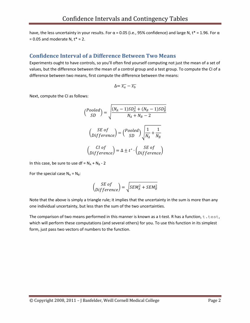
Confidence Interval of a Difference Between Two Means Experiments ought to have controls, so you’ll often find yourself computing not just the mean of a set of values, but the difference between the mean of a control group and a test group. To compute the CI of a difference between two means, first compute the difference between the means:

∆= 𝑥𝑥𝑎𝑎�� − 𝑥𝑥𝑏𝑏��

Next, compute the CI as follows:

�𝑃𝑃𝑃𝑃𝑃𝑃𝑃𝑃𝑃𝑃𝑃𝑃𝑆𝑆𝑆𝑆 � = �(𝑁𝑁𝐴𝐴 − 1)𝑆𝑆𝑆𝑆𝐴𝐴2 + (𝑁𝑁𝐵𝐵 − 1)𝑆𝑆𝑆𝑆𝐵𝐵2

𝑁𝑁𝐴𝐴 +𝑁𝑁𝐵𝐵 − 2

� 𝑆𝑆𝑆𝑆 𝑃𝑃𝑜𝑜𝑆𝑆𝐷𝐷𝑜𝑜𝑜𝑜𝑃𝑃𝐷𝐷𝑃𝑃𝐷𝐷𝐷𝐷𝑃𝑃� = �𝑃𝑃𝑃𝑃𝑃𝑃𝑃𝑃𝑃𝑃𝑃𝑃𝑆𝑆𝑆𝑆 ��

1𝑁𝑁𝐴𝐴

+1𝑁𝑁𝐵𝐵

� 𝐶𝐶𝐶𝐶 𝑃𝑃𝑜𝑜𝑆𝑆𝐷𝐷𝑜𝑜𝑜𝑜𝑃𝑃𝐷𝐷𝑃𝑃𝐷𝐷𝐷𝐷𝑃𝑃� = ∆ ± 𝑡𝑡∗ ∙ � 𝑆𝑆𝑆𝑆 𝑃𝑃𝑜𝑜

𝑆𝑆𝐷𝐷𝑜𝑜𝑜𝑜𝑃𝑃𝐷𝐷𝑃𝑃𝐷𝐷𝐷𝐷𝑃𝑃�

In this case, be sure to use df = NA + NB - 2

For the special case NA = NB:

� 𝑆𝑆𝑆𝑆 𝑃𝑃𝑜𝑜𝑆𝑆𝐷𝐷𝑜𝑜𝑜𝑜𝑃𝑃𝐷𝐷𝑃𝑃𝐷𝐷𝐷𝐷𝑃𝑃� = �𝑆𝑆𝑆𝑆𝑆𝑆𝐴𝐴

2 + 𝑆𝑆𝑆𝑆𝑆𝑆𝐵𝐵2

Note that the above is simply a triangle rule; it implies that the uncertainty in the sum is more than any one individual uncertainty, but less than the sum of the two uncertainties.

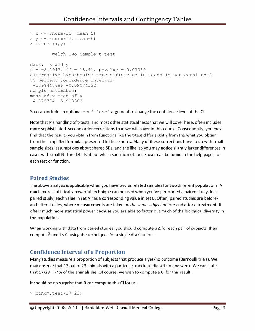
The comparison of two means performed in this manner is known as a t-test. R has a function, t.test, which will perform these computations (and several others) for you. To use this function in its simplest form, just pass two vectors of numbers to the function.



> x <- rnorm(10, mean=5) > y <- rnorm(12, mean=6) > t.test(x,y) Welch Two Sample t-test data: x and y t = -2.2943, df = 18.91, p-value = 0.03339 alternative hypothesis: true difference in means is not equal to 0 95 percent confidence interval: -1.98447686 -0.09074122 sample estimates: mean of x mean of y 4.875774 5.913383

You can include an optional conf.level argument to change the confidence level of the CI.

Note that R’s handling of t-tests, and most other statistical tests that we will cover here, often includes more sophisticated, second order corrections than we will cover in this course. Consequently, you may find that the results you obtain from functions like the t-test differ slightly from the what you obtain from the simplified formulae presented in these notes. Many of these corrections have to do with small sample sizes, assumptions about shared SDs, and the like, so you may notice slightly larger differences in cases with small N. The details about which specific methods R uses can be found in the help pages for each test or function.

Paired Studies The above analysis is applicable when you have two unrelated samples for two different populations. A much more statistically powerful technique can be used when you’ve performed a paired study. In a paired study, each value in set A has a corresponding value in set B. Often, paired studies are before-and-after studies, where measurements are taken on the same subject before and after a treatment. It offers much more statistical power because you are able to factor out much of the biological diversity in the population.

When working with data from paired studies, you should compute a Δ for each pair of subjects, then compute ∆� and its CI using the techniques for a single distribution.

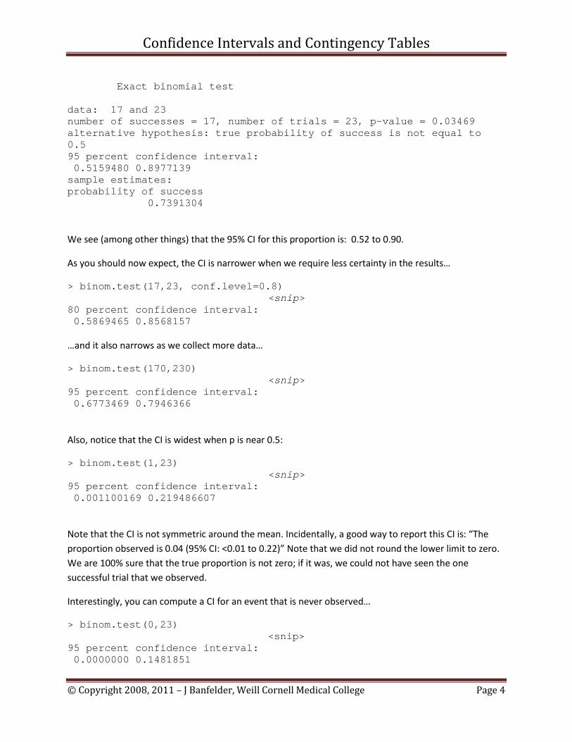
Confidence Interval of a Proportion Many studies measure a proportion of subjects that produce a yes/no outcome (Bernoulli trials). We may observe that 17 out of 23 animals with a particular knockout die within one week. We can state that 17/23 = 74% of the animals die. Of course, we wish to compute a CI for this result.

It should be no surprise that R can compute this CI for us:

> binom.test(17,23)



Exact binomial test data: 17 and 23 number of successes = 17, number of trials = 23, p-value = 0.03469 alternative hypothesis: true probability of success is not equal to 0.5 95 percent confidence interval: 0.5159480 0.8977139 sample estimates: probability of success 0.7391304

We see (among other things) that the 95% CI for this proportion is: 0.52 to 0.90.

As you should now expect, the CI is narrower when we require less certainty in the results…

> binom.test(17,23, conf.level=0.8) <snip>

80 percent confidence interval: 0.5869465 0.8568157 …and it also narrows as we collect more data…

> binom.test(170,230) <snip>

95 percent confidence interval: 0.6773469 0.7946366

Also, notice that the CI is widest when p is near 0.5:



Note that the CI is not symmetric around the mean. Incidentally, a good way to report this CI is: “The proportion observed is 0.04 (95% CI: <0.01 to 0.22)” Note that we did not round the lower limit to zero. We are 100% sure that the true proportion is not zero; if it was, we could not have seen the one successful trial that we observed.

Interestingly, you can compute a CI for an event that is never observed…





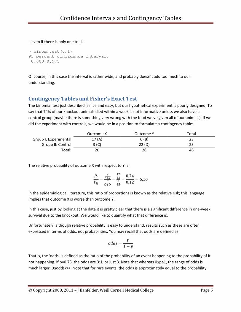
…even if there is only one trial…

> binom.test(0,1) 95 percent confidence interval: 0.000 0.975

Of course, in this case the interval is rather wide, and probably doesn’t add too much to our understanding.

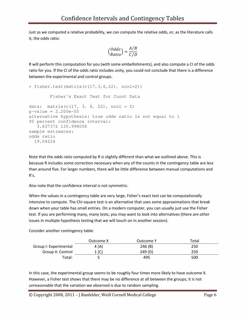
Contingency Tables and Fisher’s Exact Test The binomial test just described is nice and easy, but our hypothetical experiment is poorly designed. To say that 74% of our knockout animals died within a week is not informative unless we also have a control group (maybe there is something very wrong with the food we’ve given all of our animals). If we did the experiment with controls, we would be in a position to formulate a contingency table:

Outcome X Outcome Y Total Group I: Experimental 17 (A) 6 (B) 23

Group II: Control 3 (C) 22 (D) 25 Total: 20 28 48

The relative probability of outcome X with respect to Y is:

𝑃𝑃𝐶𝐶𝑃𝑃𝐶𝐶𝐶𝐶

=𝐴𝐴

𝐴𝐴+𝐵𝐵𝐶𝐶

𝐶𝐶+𝑆𝑆=

17233

25=

0.740.12

= 6.16

In the epidemiological literature, this ratio of proportions is known as the relative risk; this language implies that outcome X is worse than outcome Y.

In this case, just by looking at the data it is pretty clear that there is a significant difference in one-week survival due to the knockout. We would like to quantify what that difference is.

Unfortunately, although relative probability is easy to understand, results such as these are often expressed in terms of odds, not probabilities. You may recall that odds are defined as:

𝑃𝑃𝑃𝑃𝑃𝑃𝑜𝑜 =𝑝𝑝

1 − 𝑝𝑝

That is, the ‘odds’ is defined as the ratio of the probability of an event happening to the probability of it not happening. If p=0.75, the odds are 3:1, or just 3. Note that whereas 0≤p≤1, the range of odds is much larger: 0≤odds<∞. Note that for rare events, the odds is approximately equal to the probability.



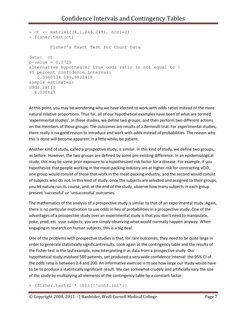
Just as we computed a relative probability, we can compute the relative odds, or, as the literature calls it, the odds ratio:

�𝑂𝑂𝑃𝑃𝑃𝑃𝑜𝑜𝑅𝑅𝑎𝑎𝑡𝑡𝐷𝐷𝑃𝑃� =𝐴𝐴 𝐵𝐵⁄𝐶𝐶 𝑆𝑆⁄

R will perform this computation for you (with some embellishments), and also compute a CI of the odds ratio for you. If the CI of the odds ratio includes unity, you could not conclude that there is a difference between the experimental and control groups.

> fisher.test(matrix(c(17,3,6,22), ncol=2)) Fisher's Exact Test for Count Data data: matrix(c(17, 3, 6, 22), ncol = 2) p-value = 2.200e-05 alternative hypothesis: true odds ratio is not equal to 1 95 percent confidence interval: 3.837372 135.998058 sample estimates: odds ratio 19.04224

Note that the odds ratio computed by R is slightly different than what we outlined above. This is because R includes some correction necessary when any of the counts in the contingency table are less than around five. For larger numbers, there will be little difference between manual computations and R’s.

Also note that the confidence interval is not symmetric.

When the values in a contingency table are very large, Fisher’s exact test can be computationally intensive to compute. The Chi-square test is an alternative that uses some approximations that break down when your table has small entries. On a modern computer, you can usually just use the Fisher test. If you are performing many, many tests, you may want to look into alternatives (there are other issues in multiple hypothesis testing that we will touch on in another session).

Consider another contingency table:

Outcome X Outcome Y Total Group I: Experimental 4 (A) 246 (B) 250

Group II: Control 1 (C) 249 (D) 250 Total: 5 495 500

In this case, the experimental group seems to be roughly four times more likely to have outcome X. However, a Fisher test shows that there may be no difference at all between the groups; it is not unreasonable that the variation we observed is due to random sampling.



> ct <- matrix(c(4,1,246,249), ncol=2) > fisher.test(ct) Fisher's Exact Test for Count Data data: ct p-value = 0.3725 alternative hypothesis: true odds ratio is not equal to 1 95 percent confidence interval: 0.3960534 199.9822418 sample estimates: odds ratio 4.038627

At this point, you may be wondering why we have elected to work with odds ratios instead of the more natural relative proportions. Thus far, all of our hypothetical examples have been of what are termed ‘experimental studies’. In these studies, we define two groups, and then perform two different actions on the members of those groups. The outcomes are results of a Bernoulli trial. For experimental studies, there really is no good reason to introduce and work with odds instead of probabilities. The reason why this is done will become apparent in a little while; be patient.

Another kind of study, called a prospective study, is similar. In this kind of study, we define two groups, as before. However, the two groups are defined by some pre-existing difference. In an epidemiological study, this may be some prior exposure to a hypothesized risk factor for a disease. For example, if you hypothesize that people working in the meat-packing industry are at higher risk for contracting vCJD, one group would consist of those that work in the meat-packing industry, and the second would consist of subjects who do not. In this kind of study, once the subjects are selected and assigned to their groups, you let nature run its course, and, at the end of the study, observe how many subjects in each group present ‘successful’ or ‘unsuccessful’ outcomes.

The mathematics of the analysis of a prospective study is similar to that of an experimental study. Again, there is no particular motivation to use odds in lieu of probabilities in a prospective study. One of the advantages of a prospective study over an experimental study is that you don’t need to manipulate, poke, prod, etc. your subjects; you are simply observing what would normally happen anyway. When engaging in research on human subjects, this is a big deal.

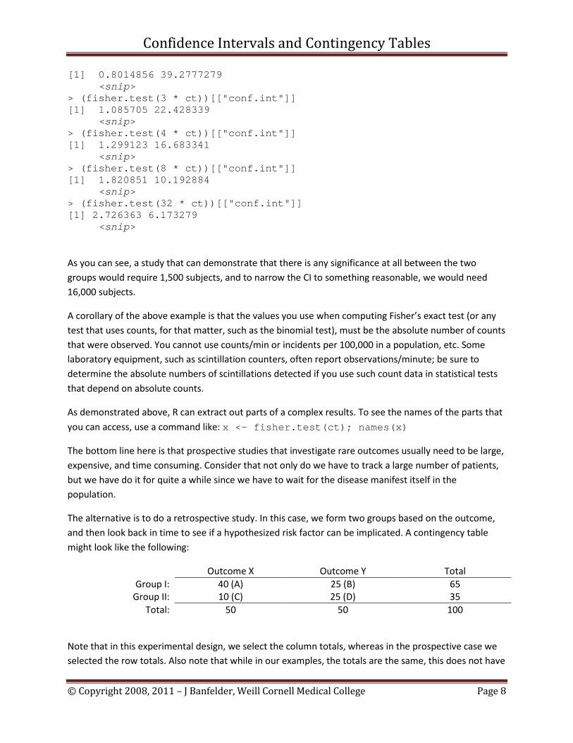
One of the problems with prospective studies is that, for rare outcomes, they need to be quite large in order to generate statistically significant results. Look again at the contingency table and the results of the Fisher test in the last example, now interpreting it as data from a prospective study. Our hypothetical study involved 500 patients, yet produced a very wide confidence interval: the 95% CI of the odds ratio is between 0.4 and 200. An informative exercise is to see how large our study would have to be to produce a statistically significant result. We can somewhat crudely and artificially vary the size of the study by multiplying all elements of the contingency table by a constant factor:

> (fisher.test(2 * ct))[["conf.int"]]



[1] 0.8014856 39.2777279 <snip> > (fisher.test(3 * ct))[["conf.int"]] [1] 1.085705 22.428339 <snip> > (fisher.test(4 * ct))[["conf.int"]] [1] 1.299123 16.683341 <snip> > (fisher.test(8 * ct))[["conf.int"]] [1] 1.820851 10.192884 <snip> > (fisher.test(32 * ct))[["conf.int"]] [1] 2.726363 6.173279 <snip>

As you can see, a study that can demonstrate that there is any significance at all between the two groups would require 1,500 subjects, and to narrow the CI to something reasonable, we would need 16,000 subjects.

A corollary of the above example is that the values you use when computing Fisher’s exact test (or any test that uses counts, for that matter, such as the binomial test), must be the absolute number of counts that were observed. You cannot use counts/min or incidents per 100,000 in a population, etc. Some laboratory equipment, such as scintillation counters, often report observations/minute; be sure to determine the absolute numbers of scintillations detected if you use such count data in statistical tests that depend on absolute counts.

As demonstrated above, R can extract out parts of a complex results. To see the names of the parts that you can access, use a command like: x <- fisher.test(ct); names(x)

The bottom line here is that prospective studies that investigate rare outcomes usually need to be large, expensive, and time consuming. Consider that not only do we have to track a large number of patients, but we have do it for quite a while since we have to wait for the disease manifest itself in the population.

The alternative is to do a retrospective study. In this case, we form two groups based on the outcome, and then look back in time to see if a hypothesized risk factor can be implicated. A contingency table might look like the following:

Outcome X Outcome Y Total Group I: 40 (A) 25 (B) 65

Group II: 10 (C) 25 (D) 35 Total: 50 50 100

Note that in this experimental design, we select the column totals, whereas in the prospective case we selected the row totals. Also note that while in our examples, the totals are the same, this does not have



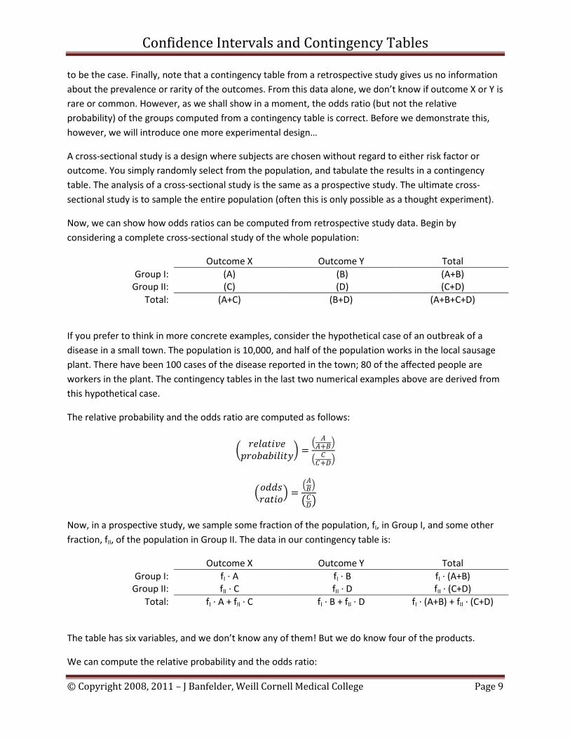
to be the case. Finally, note that a contingency table from a retrospective study gives us no information about the prevalence or rarity of the outcomes. From this data alone, we don’t know if outcome X or Y is rare or common. However, as we shall show in a moment, the odds ratio (but not the relative probability) of the groups computed from a contingency table is correct. Before we demonstrate this, however, we will introduce one more experimental design…

A cross-sectional study is a design where subjects are chosen without regard to either risk factor or outcome. You simply randomly select from the population, and tabulate the results in a contingency table. The analysis of a cross-sectional study is the same as a prospective study. The ultimate cross-sectional study is to sample the entire population (often this is only possible as a thought experiment).

Now, we can show how odds ratios can be computed from retrospective study data. Begin by considering a complete cross-sectional study of the whole population:

Outcome X Outcome Y Total Group I: (A) (B) (A+B)

Group II: (C) (D) (C+D) Total: (A+C) (B+D) (A+B+C+D)

If you prefer to think in more concrete examples, consider the hypothetical case of an outbreak of a disease in a small town. The population is 10,000, and half of the population works in the local sausage plant. There have been 100 cases of the disease reported in the town; 80 of the affected people are workers in the plant. The contingency tables in the last two numerical examples above are derived from this hypothetical case.

The relative probability and the odds ratio are computed as follows:

� 𝐷𝐷𝑃𝑃𝑃𝑃𝑎𝑎𝑡𝑡𝐷𝐷𝑟𝑟𝑃𝑃𝑝𝑝𝐷𝐷𝑃𝑃𝑏𝑏𝑎𝑎𝑏𝑏𝐷𝐷𝑃𝑃𝐷𝐷𝑡𝑡𝑝𝑝� =

� 𝐴𝐴𝐴𝐴+𝐵𝐵�

� 𝐶𝐶𝐶𝐶+𝑆𝑆�

�𝑃𝑃𝑃𝑃𝑃𝑃𝑜𝑜𝐷𝐷𝑎𝑎𝑡𝑡𝐷𝐷𝑃𝑃� =�𝐴𝐴𝐵𝐵�

�𝐶𝐶𝑆𝑆�

Now, in a prospective study, we sample some fraction of the population, fI, in Group I, and some other fraction, fII, of the population in Group II. The data in our contingency table is:

Outcome X Outcome Y Total Group I: fI ∙ A fI ∙ B fI ∙ (A+B)

Group II: fII ∙ C fII ∙ D fII ∙ (C+D) Total: fI ∙ A + fII ∙ C fI ∙ B + fII ∙ D fI ∙ (A+B) + fII ∙ (C+D)

The table has six variables, and we don’t know any of them! But we do know four of the products.

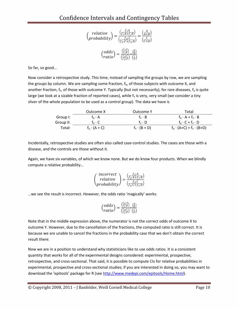
We can compute the relative probability and the odds ratio:



� 𝐷𝐷𝑃𝑃𝑃𝑃𝑎𝑎𝑡𝑡𝐷𝐷𝑟𝑟𝑃𝑃𝑝𝑝𝐷𝐷𝑃𝑃𝑏𝑏𝑎𝑎𝑏𝑏𝐷𝐷𝑃𝑃𝐷𝐷𝑡𝑡𝑝𝑝� =

� 𝑜𝑜𝐶𝐶𝐴𝐴𝑜𝑜𝐶𝐶𝐴𝐴+𝑜𝑜𝐶𝐶𝐵𝐵

�

� 𝑜𝑜𝐶𝐶𝐶𝐶 𝐶𝐶𝑜𝑜𝐶𝐶𝐶𝐶𝐶𝐶+𝑜𝑜𝐶𝐶𝐶𝐶𝑆𝑆

�=

� 𝐴𝐴𝐴𝐴+𝐵𝐵�

� 𝐶𝐶𝐶𝐶+𝑆𝑆�

�𝑃𝑃𝑃𝑃𝑃𝑃𝑜𝑜𝐷𝐷𝑎𝑎𝑡𝑡𝐷𝐷𝑃𝑃� =�𝑜𝑜𝐶𝐶𝐴𝐴𝑜𝑜𝐶𝐶𝐵𝐵

�

�𝑜𝑜𝐶𝐶𝐶𝐶𝐶𝐶𝑜𝑜𝐶𝐶𝐶𝐶𝑆𝑆�=�𝐴𝐴𝐵𝐵�


So far, so good…

Now consider a retrospective study. This time, instead of sampling the groups by row, we are sampling the groups by column. We are sampling some fraction, fX, of those subjects with outcome X, and another fraction, fY, of those with outcome Y. Typically (but not necessarily), for rare diseases, fX is quite large (we look at a sizable fraction of reported cases), while fY is very, very small (we consider a tiny sliver of the whole population to be used as a control group). The data we have is

Outcome X Outcome Y Total Group I: fX ∙ A fY ∙ B fX ∙ A + fY ∙ B

Group II: fX ∙ C fY ∙ D fX ∙ C + fY ∙ D Total: fX ∙ (A + C) fY ∙ (B + D) fX ∙ (A+C) + fY ∙ (B+D)

Incidentally, retrospective studies are often also called case-control studies. The cases are those with a disease, and the controls are those without it.

Again, we have six variables, of which we know none. But we do know four products. When we blindly compute a relative probability…

�𝐷𝐷𝐷𝐷𝐷𝐷𝑃𝑃𝐷𝐷𝐷𝐷𝑃𝑃𝐷𝐷𝑡𝑡𝐷𝐷𝑃𝑃𝑃𝑃𝑎𝑎𝑡𝑡𝐷𝐷𝑟𝑟𝑃𝑃

𝑝𝑝𝐷𝐷𝑃𝑃𝑏𝑏𝑎𝑎𝑏𝑏𝐷𝐷𝑃𝑃𝐷𝐷𝑡𝑡𝑝𝑝� =

� 𝑜𝑜𝑋𝑋 𝐴𝐴𝑜𝑜𝑋𝑋 𝐴𝐴+𝑜𝑜𝑌𝑌𝐵𝐵

�

� 𝑜𝑜𝑋𝑋𝐶𝐶𝑜𝑜𝑋𝑋𝐶𝐶+𝑜𝑜𝑌𝑌𝑆𝑆

�

…we see the result is incorrect. However, the odds ratio ‘magically’ works:

�𝑃𝑃𝑃𝑃𝑃𝑃𝑜𝑜𝐷𝐷𝑎𝑎𝑡𝑡𝐷𝐷𝑃𝑃� =�𝑜𝑜𝑋𝑋 𝐴𝐴𝑜𝑜𝑌𝑌𝐵𝐵

�

�𝑜𝑜𝑋𝑋 𝐶𝐶𝑜𝑜𝑌𝑌𝑆𝑆�=�𝐴𝐴𝐵𝐵�


Note that in the middle expression above, the numerator is not the correct odds of outcome X to outcome Y. However, due to the cancellation of the fractions, the computed ratio is still correct. It is because we are unable to cancel the fractions in the probability case that we don’t obtain the correct result there.

Now we are in a position to understand why statisticians like to use odds ratios. It is a consistent quantity that works for all of the experimental designs considered: experimental, prospective, retrospective, and cross-sectional. That said, it is possible to compute CIs for relative probabilities in experimental, prospective and cross-sectional studies; if you are interested in doing so, you may want to download the ‘epitools’ package for R (see http://www.medepi.com/epitools/Home.html).

http://www.medepi.com/epitools/Home.html



Recall that for rare diseases, the odds are approximately the same as the probability. So, for rare diseases, as a bonus, you can use the odds ratio from a retrospective study as a good approximation for a relative probability (aka relative risk).

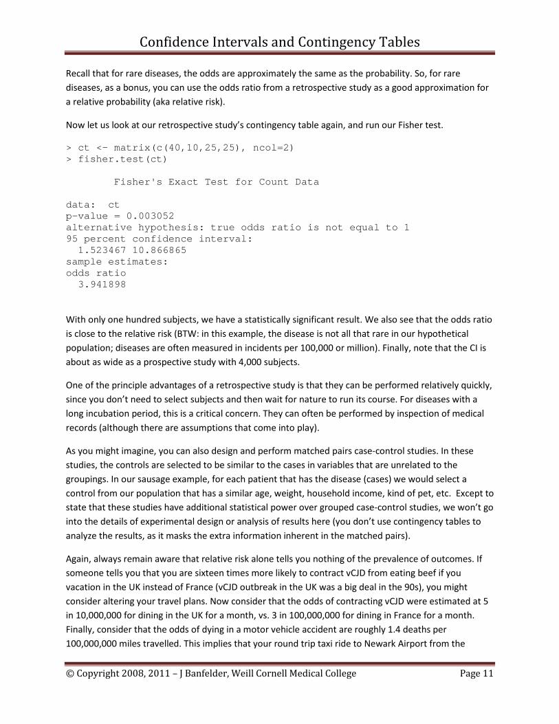
Now let us look at our retrospective study’s contingency table again, and run our Fisher test.

> ct <- matrix(c(40,10,25,25), ncol=2) > fisher.test(ct) Fisher's Exact Test for Count Data data: ct p-value = 0.003052 alternative hypothesis: true odds ratio is not equal to 1 95 percent confidence interval: 1.523467 10.866865 sample estimates: odds ratio 3.941898

With only one hundred subjects, we have a statistically significant result. We also see that the odds ratio is close to the relative risk (BTW: in this example, the disease is not all that rare in our hypothetical population; diseases are often measured in incidents per 100,000 or million). Finally, note that the CI is about as wide as a prospective study with 4,000 subjects.

One of the principle advantages of a retrospective study is that they can be performed relatively quickly, since you don’t need to select subjects and then wait for nature to run its course. For diseases with a long incubation period, this is a critical concern. They can often be performed by inspection of medical records (although there are assumptions that come into play).

As you might imagine, you can also design and perform matched pairs case-control studies. In these studies, the controls are selected to be similar to the cases in variables that are unrelated to the groupings. In our sausage example, for each patient that has the disease (cases) we would select a control from our population that has a similar age, weight, household income, kind of pet, etc. Except to state that these studies have additional statistical power over grouped case-control studies, we won’t go into the details of experimental design or analysis of results here (you don’t use contingency tables to analyze the results, as it masks the extra information inherent in the matched pairs).

Again, always remain aware that relative risk alone tells you nothing of the prevalence of outcomes. If someone tells you that you are sixteen times more likely to contract vCJD from eating beef if you vacation in the UK instead of France (vCJD outbreak in the UK was a big deal in the 90s), you might consider altering your travel plans. Now consider that the odds of contracting vCJD were estimated at 5 in 10,000,000 for dining in the UK for a month, vs. 3 in 100,000,000 for dining in France for a month. Finally, consider that the odds of dying in a motor vehicle accident are roughly 1.4 deaths per 100,000,000 miles travelled. This implies that your round trip taxi ride to Newark Airport from the



Medical College is a bit more risky than your exposure to vCJD would have been in the UK. This is not to say that we shouldn’t protect our food supply (left unchecked, the odds may have gotten a lot worse) or avoid risky behaviors, but it is important to keep things in perspective.

Further Reading Harvey Mutolsky’s excellent book, Intuitive Biostatistics, has been the inspiration for much of the material in this section (http://www.amazon.com/Intuitive-Biostatistics-Harvey-Motulsky/dp/0195086074/).

http://www.amazon.com/Intuitive-Biostatistics-Harvey-Motulsky/dp/0195086074/

http://www.amazon.com/Intuitive-Biostatistics-Harvey-Motulsky/dp/0195086074/

confidence intervals and contingency tables -...

Documents