Journal of Hydrology 486 (2013) 321–333

Contents lists available at SciVerse ScienceDirect

Journal of Hydrology

journal homepage: www.elsevier .com/ locate / jhydrol

Conditions for lateral downslope unsaturated flow and effects of slope angleon soil moisture movement

Meixia Lv a,⇑, Zhenchun Hao a, Zhen Liu a, Zhongbo Yu a,b

a State Key Laboratory of Hydrology-Water Resources and Hydraulic Engineering, Hohai University, Nanjing 210098, Chinab Department of Geoscience, University of Nevada, Las Vegas, NV, United States

a r t i c l e i n f o s u m m a r y

Article history:Received 27 November 2012Received in revised form 29 January 2013Accepted 2 February 2013Available online 18 February 2013This manuscript was handled by CorradoCorradini, Editor-in-Chief, with theassistance of Rao S. Govindaraju, AssociateEditor

Keywords:Lateral downslope flowUnsaturated zoneSlope anglesSoil moisture movement

0022-1694/$ - see front matter � 2013 Elsevier B.V. Ahttp://dx.doi.org/10.1016/j.jhydrol.2013.02.013

⇑ Corresponding author. Address: State Key LabResources and Hydraulic Engineering, Hohai Univer210098, China. Tel.: +86 18710186950; fax: +86 25 8

E-mail address: MeixiaLv22@gmail.com (M. Lv).

The necessary conditions for lateral downslope flow in the unsaturated zone in hillslopes have not beenclearly identified, and the effects of different slope angles on soil moisture movement are rarely studied.These questions were investigated through drying processes in a homogeneous and isotropic sloping soiltank in this study. Three experiments with different slope angles were conducted. The results showedthat the flow direction in the unsaturated zone gradually rotates counterclockwise from the verticaldirection to the lateral downslope direction parallel to the slope surface during the drying phase. The lat-eral downslope flow parallel to the slope surface first appears at the surface (0–5 cm) and the bottom ofthe sandy loam in the tank. The lateral downslope flow parallel to the slope surface at the surface is dueto the state of drying rather than the no-flow upper boundary condition. The lateral downslope flow par-allel to the slope surface at the bottom of the sandy loam is also caused by the state of drying. Moreimportantly, the results of this study showed that the rate at which the lateral downslope flow turnsto be parallel to the slope surface is affected by the drainage rate. In contrast to the lateral downslopeflow component parallel to the slope surface, the flow component normal to the slope surface is less sen-sitive to changes in the slope angle. The influence of the slope angle on the flow component normal to theslope surface is greatest in the middle layer.

� 2013 Elsevier B.V. All rights reserved.

1. Introduction

Lateral downslope water flows in both saturated and unsatu-rated zones, which could affect the redistribution of soil moisture,are important (Genereux and Hemond, 1990). Perry and Niemann(2007) found that two important factors influence soil moisturespatial patterns whose individual effects vary with time: lateralredistribution of soil moisture and evapotranspiration. Graysonet al. (1997) found that lateral flow is the controlling factor inthe wet state of soil moisture, while vertical flow is the controllingfactor for the dry state. Among the factors affecting the variabilityof soil moisture in the Southern Great Plains 1997 (SGP97) fieldcampaign, Jawson and Niemann (2007) found that there weremoderate correlations between slope angle and the primary pat-terns from empirical orthogonal function analysis (EOFs), whileno correlations were found between the topographic curvatureand EOFs. However, a clear relation remains to be determined.Yoo and Kim (2004) claimed that topography-related factors weresignificantly correlated with EOFs at a smaller scale in the same

ll rights reserved.

oratory of Hydrology-Watersity, 1 Xikang Road, Nanjing3786614.

region. Jawson and Niemann (2007) suspected that the oppositeresults were most likely due to lateral flow, whose effect on soilmoisture redistribution was unlikely to be observed at the finestscales in their research.

Hillslope hydrology has been a topic of much research interestin the past few decades (e.g., Bronstert, 1999; Kirkby, 1978; Wes-tern and Grayson, 1998). Studies have shown that lateral unsatu-rated flow does occur in hillslopes (Kim et al., 2005; McCordet al., 1991), even though the soil is homogeneous and isotropic(Jackson, 1992; Lu et al., 2011; Ridolfi et al., 2003; Sinai and Dirk-sen, 2006). For instance, McCord and Stephens (1987) found thatsubsurface lateral flow in the unsaturated zone can occur even ina sandy hillslope without low-permeability sublayers. Many stud-ies have demonstrated that lateral downslope unsaturated flow oc-curs during the drying phase (e.g., Pan et al., 1997; Sinai andDirksen, 2006).

However, the necessary conditions for lateral downslope unsat-urated flow in hillslopes still have not been clearly identified. Jack-son (1992) noted that it is the no-flow boundary condition at thesoil surface that forces soil moisture to move in the direction par-allel to the boundary. It has been well established that anisotropyand layering can promote the occurrence of lateral downslope flow(Miyazaki, 1988; Warrick et al., 1997). In contrast, Sinai and Dirk-sen (2006) suggested that the necessary condition for lateral

322 M. Lv et al. / Journal of Hydrology 486 (2013) 321–333

downslope flow is decreasing rain intensity rather than the no-flow boundary condition, anisotropy or layering. However, Luet al. (2011) commented that Sinai and Dirksen’s (2006) attributionof the necessary condition to rainfall at the surface was unreason-able, and they proposed a new mechanism, according to which ‘‘atany point within a homogeneous and isotropic hillslope, down-slope lateral unsaturated flow will occur if that point is in the stateof drying.’’ The viewpoints of Sinai and Dirksen (2006) and Lu et al.(2011) have something in common concerning when lateral down-slope flow occurs: under the two conditions, decreasing rain inten-sity or a drying state, the same pattern for the vertical soil waterpotential gradient is formed, i.e., ow/oz < 0. Kim et al. (2011) foundthat vertical infiltration is mainly responsible for the hydrologicprocesses in the upper soil layer and that the soil moisture behav-ior in the lower soil layer is likely to be controlled by lateral redis-tribution. However, Kim et al. (2011) found that the moisturevariation with time were similar at depths of 10 cm, 30 cm and60 cm below the surface, i.e., decreasing slightly. It should be notedthat Kim et al. (2011) did not divide the study period into during-rainfall and after-rainfall sub-periods but rather treated it as awhole. On the other hand, after rainfalls ceased, soil moisture rap-idly fell to its original level, and thus the soil moisture trend did notvary throughout the observation period in their research.

There are two commonly used definitions of upslope and down-slope soil moisture flows. One takes the direction normal to theslope surface as the divide (Philip, 1991), and the other uses thevertical direction as the divide (Jackson, 1992), which is consideredto be more reasonable (Lu et al., 2011). Therefore, we use the ver-tical direction as the divide in this paper, i.e., the direction ofdownslope flow is from the vertical direction to the slope surface,and the direction normal to the slope surface belongs to the ups-lope (Fig. 1).

Several studies have shown that the slope angle plays an impor-tant role in the distribution of soil moisture (Kim, 2009; Svetlitch-nyi et al., 2003). The influence of slope angle on the soil moisturedistribution has been examined in many studies (e.g., Pat andEltahir, 1998; Philip, 1991; Tromp-van Meerveld and McDonnell,2006). Kim and Kim (2007) employed the topographic wetness in-dex (ln (a/tanb)) to explore the stochastic structure of soil mois-ture on a steep hillside, but they did not investigate how theslope angle affects the distribution of soil moisture. AlthoughSvetlitchnyi et al. (2003) proposed a scheme to explain the effectof slope angle on evaporation and hence soil moisture, they didnot describe the direct relationship between slope angle and soilmoisture distribution, and they paid little attention to the effectsof different slope angles. Penna et al. (2009) analyzed soil moisturevariability in three natural hillslopes with slope ranges of 21–84%,21–90% and 25–90%. However, these hillslopes had remarkablydistinct relief shapes, so the effect of slope angles was not isolatedin their study. Morbidelli et al. (2008) investigated the infiltrationof surface water running downslope from upstream at slope anglesof 1�, 5� and 10�. Essig et al. (2009) found that surface flowincreases with increasing slope angle on the sloping surface. These

Fig. 1. Definition of downslope and upslope flow directions.

two studies did not offer much discussion of the lateral movementof soil moisture.

Therefore, the primary objectives of this study were to investi-gate the following: (1) the necessary conditions for lateral down-slope flow in the unsaturated zone and (2) the effects of differentslope angles on soil moisture movement. The study was conductedvia laboratory experiments at three slope angles 9�, 19� and 28�,which were selected to cover all possible angles of hillslopes innature to the greatest extent possible. Numerical modeling wasalso conducted because of the lack of observations in the shallowsoil layers at 0–5 cm. This paper is organized as follows: first, thedesign of the laboratory experiments, numerical modeling andanalysis methods are briefly described. Then, the dynamics of theflow direction are examined based on the soil water potential mea-sured in the laboratory experiments and the microscopic processessimulated with HYDRUS-2D. Finally, comparisons are presented forthe different slope angles considered based on the experimentalresults.

2. Materials and methods

2.1. Laboratory experiments

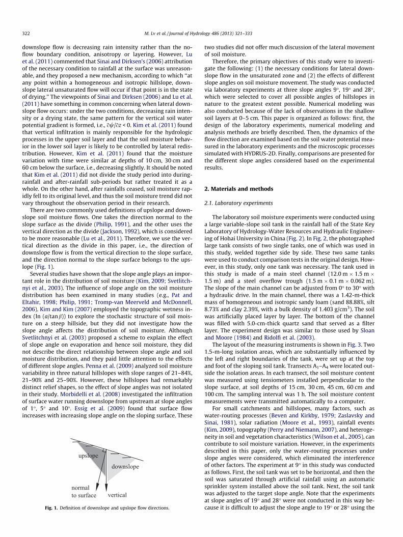
The laboratory soil moisture experiments were conducted usinga large variable-slope soil tank in the rainfall hall of the State KeyLaboratory of Hydrology-Water Resources and Hydraulic Engineer-ing of Hohai University in China (Fig. 2). In Fig. 2, the photographedlarge tank consists of two single tanks, one of which was used inthis study, welded together side by side. These two same tankswere used to conduct comparison tests in the original design. How-ever, in this study, only one tank was necessary. The tank used inthis study is made of a main steel channel (12.0 m � 1.5 m �1.5 m) and a steel overflow trough (1.5 m � 0.1 m � 0.062 m).The slope of the main channel can be adjusted from 0� to 30� witha hydraulic drive. In the main channel, there was a 1.42-m-thickmass of homogeneous and isotropic sandy loam (sand 88.88%, silt8.73% and clay 2.39%, with a bulk density of 1.403 g/cm3). The soilwas artificially placed layer by layer. The bottom of the channelwas filled with 5.0-cm-thick quartz sand that served as a filterlayer. The experiment design was similar to those used by Sloanand Moore (1984) and Ridolfi et al. (2003).

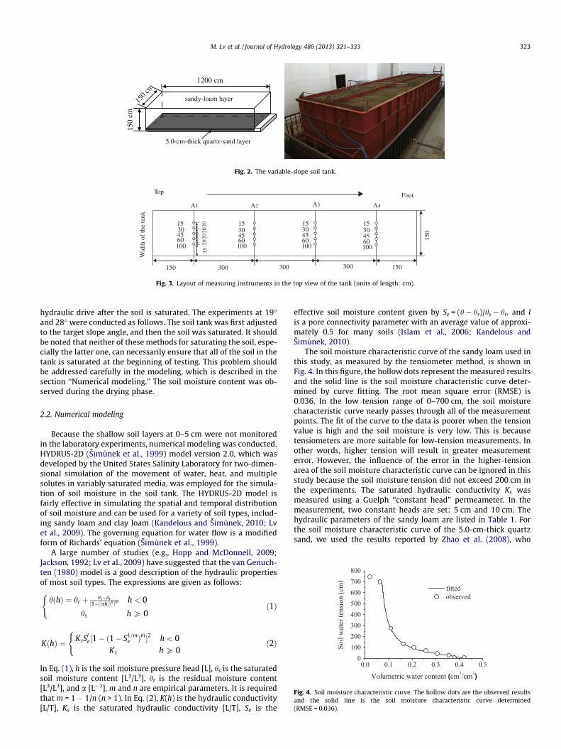
The layout of the measuring instruments is shown in Fig. 3. Two1.5-m-long isolation areas, which are substantially influenced bythe left and right boundaries of the tank, were set up at the topand foot of the sloping soil tank. Transects A1–A4 were located out-side the isolation areas. In each transect, the soil moisture contentwas measured using tensiometers installed perpendicular to theslope surface, at soil depths of 15 cm, 30 cm, 45 cm, 60 cm and100 cm. The sampling interval was 1 h. The soil moisture contentmeasurements were transmitted automatically to a computer.

For small catchments and hillslopes, many factors, such aswater-routing processes (Beven and Kirkby, 1979; Zaslavsky andSinai, 1981), solar radiation (Moore et al., 1993), rainfall events(Kim, 2009), topography (Perry and Niemann, 2007), and heteroge-neity in soil and vegetation characteristics (Wilson et al., 2005), cancontribute to soil moisture variation. However, in the experimentsdescribed in this paper, only the water-routing processes underslope angles were considered, which eliminated the interferenceof other factors. The experiment at 9� in this study was conductedas follows. First, the soil tank was set to be horizontal, and then thesoil was saturated through artificial rainfall using an automaticsprinkler system installed above the soil tank. Next, the soil tankwas adjusted to the target slope angle. Note that the experimentsat slope angles of 19� and 28� were not conducted in this way be-cause it is difficult to adjust the slope angle to 19� or 28� using the

1200 cm

150 c

m

150

cm

sandy-loam layer

5.0-cm-thick quartz-sand layer

Fig. 2. The variable-slope soil tank.

15304560100

1530

6045

100

153045

100

153045

10060 60

2020

2020

35

150

150

150300 300300

A1 A4A3A2

Top Foot

Wid

th o

f th

e ta

nk

Fig. 3. Layout of measuring instruments in the top view of the tank (units of length: cm).

M. Lv et al. / Journal of Hydrology 486 (2013) 321–333 323

hydraulic drive after the soil is saturated. The experiments at 19�and 28� were conducted as follows. The soil tank was first adjustedto the target slope angle, and then the soil was saturated. It shouldbe noted that neither of these methods for saturating the soil, espe-cially the latter one, can necessarily ensure that all of the soil in thetank is saturated at the beginning of testing. This problem shouldbe addressed carefully in the modeling, which is described in thesection ‘‘Numerical modeling.’’ The soil moisture content was ob-served during the drying phase.

2.2. Numerical modeling

Because the shallow soil layers at 0–5 cm were not monitoredin the laboratory experiments, numerical modeling was conducted.HYDRUS-2D (Šimunek et al., 1999) model version 2.0, which wasdeveloped by the United States Salinity Laboratory for two-dimen-sional simulation of the movement of water, heat, and multiplesolutes in variably saturated media, was employed for the simula-tion of soil moisture in the soil tank. The HYDRUS-2D model isfairly effective in simulating the spatial and temporal distributionof soil moisture and can be used for a variety of soil types, includ-ing sandy loam and clay loam (Kandelous and Šimunek, 2010; Lvet al., 2009). The governing equation for water flow is a modifiedform of Richards’ equation (Šimunek et al., 1999).

A large number of studies (e.g., Hopp and McDonnell, 2009;Jackson, 1992; Lv et al., 2009) have suggested that the van Genuch-ten (1980) model is a good description of the hydraulic propertiesof most soil types. The expressions are given as follows:

hðhÞ ¼ hr þ hs�hr½1þðjahjÞn �m h < 0

hs h P 0

(ð1Þ

Fig. 4. Soil moisture characteristic curve. The hollow dots are the observed resultsand the solid line is the soil moisture characteristic curve determined(RMSE = 0.036).

KðhÞ ¼ KsSle½1� ð1� S1=m

e Þm�2 h < 0Ks h P 0

(ð2Þ

In Eq. (1), h is the soil moisture pressure head [L], hs is the saturatedsoil moisture content [L3/L3], hr is the residual moisture content[L3/L3], and a [L�1], m and n are empirical parameters. It is requiredthat m = 1 � 1/n (n > 1). In Eq. (2), K(h) is the hydraulic conductivity[L/T], Ks is the saturated hydraulic conductivity [L/T], Se is the

effective soil moisture content given by Se = (h � hr)/hs � hr, and lis a pore connectivity parameter with an average value of approxi-mately 0.5 for many soils (Islam et al., 2006; Kandelous andŠimunek, 2010).

The soil moisture characteristic curve of the sandy loam used inthis study, as measured by the tensiometer method, is shown inFig. 4. In this figure, the hollow dots represent the measured resultsand the solid line is the soil moisture characteristic curve deter-mined by curve fitting. The root mean square error (RMSE) is0.036. In the low tension range of 0–700 cm, the soil moisturecharacteristic curve nearly passes through all of the measurementpoints. The fit of the curve to the data is poorer when the tensionvalue is high and the soil moisture is very low. This is becausetensiometers are more suitable for low-tension measurements. Inother words, higher tension will result in greater measurementerror. However, the influence of the error in the higher-tensionarea of the soil moisture characteristic curve can be ignored in thisstudy because the soil moisture tension did not exceed 200 cm inthe experiments. The saturated hydraulic conductivity Ks wasmeasured using a Guelph ‘‘constant head’’ permeameter. In themeasurement, two constant heads are set: 5 cm and 10 cm. Thehydraulic parameters of the sandy loam are listed in Table 1. Forthe soil moisture characteristic curve of the 5.0-cm-thick quartzsand, we used the results reported by Zhao et al. (2008), who

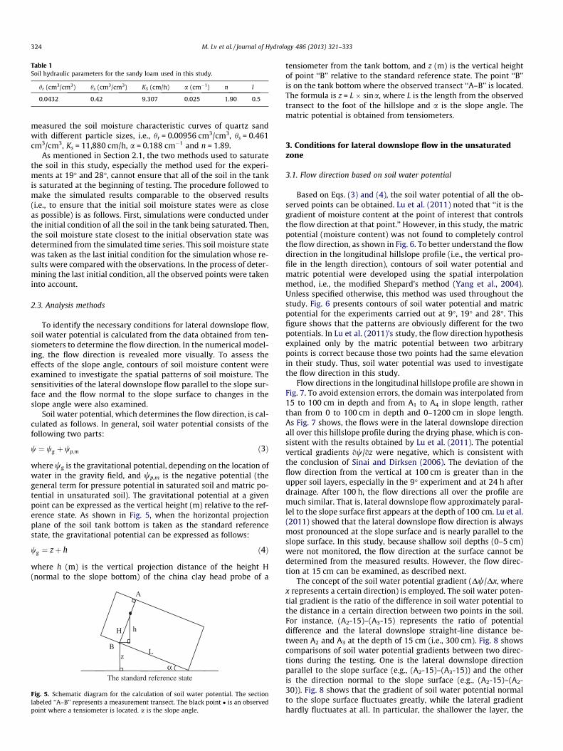
Table 1Soil hydraulic parameters for the sandy loam used in this study.

hr (cm3/cm3) hs (cm3/cm3) KS (cm/h) a (cm�1) n l

0.0432 0.42 9.307 0.025 1.90 0.5

324 M. Lv et al. / Journal of Hydrology 486 (2013) 321–333

measured the soil moisture characteristic curves of quartz sandwith different particle sizes, i.e., hr = 0.00956 cm3/cm3, hs = 0.461cm3/cm3, Ks = 11,880 cm/h, a = 0.188 cm�1 and n = 1.89.

As mentioned in Section 2.1, the two methods used to saturatethe soil in this study, especially the method used for the experi-ments at 19� and 28�, cannot ensure that all of the soil in the tankis saturated at the beginning of testing. The procedure followed tomake the simulated results comparable to the observed results(i.e., to ensure that the initial soil moisture states were as closeas possible) is as follows. First, simulations were conducted underthe initial condition of all the soil in the tank being saturated. Then,the soil moisture state closest to the initial observation state wasdetermined from the simulated time series. This soil moisture statewas taken as the last initial condition for the simulation whose re-sults were compared with the observations. In the process of deter-mining the last initial condition, all the observed points were takeninto account.

2.3. Analysis methods

To identify the necessary conditions for lateral downslope flow,soil water potential is calculated from the data obtained from ten-siometers to determine the flow direction. In the numerical model-ing, the flow direction is revealed more visually. To assess theeffects of the slope angle, contours of soil moisture content wereexamined to investigate the spatial patterns of soil moisture. Thesensitivities of the lateral downslope flow parallel to the slope sur-face and the flow normal to the slope surface to changes in theslope angle were also examined.

Soil water potential, which determines the flow direction, is cal-culated as follows. In general, soil water potential consists of thefollowing two parts:

w ¼ wg þ wp;m ð3Þ

where wg is the gravitational potential, depending on the location ofwater in the gravity field, and wp,m is the negative potential (thegeneral term for pressure potential in saturated soil and matric po-tential in unsaturated soil). The gravitational potential at a givenpoint can be expressed as the vertical height (m) relative to the ref-erence state. As shown in Fig. 5, when the horizontal projectionplane of the soil tank bottom is taken as the standard referencestate, the gravitational potential can be expressed as follows:

wg ¼ zþ h ð4Þ

where h (m) is the vertical projection distance of the height H(normal to the slope bottom) of the china clay head probe of a

A

Bz

hH

α

The standard reference state

L

Fig. 5. Schematic diagram for the calculation of soil water potential. The sectionlabeled ‘‘A–B’’ represents a measurement transect. The black point � is an observedpoint where a tensiometer is located. a is the slope angle.

tensiometer from the tank bottom, and z (m) is the vertical heightof point ‘‘B’’ relative to the standard reference state. The point ‘‘B’’is on the tank bottom where the observed transect ‘‘A–B’’ is located.The formula is z = L � sina, where L is the length from the observedtransect to the foot of the hillslope and a is the slope angle. Thematric potential is obtained from tensiometers.

3. Conditions for lateral downslope flow in the unsaturatedzone

3.1. Flow direction based on soil water potential

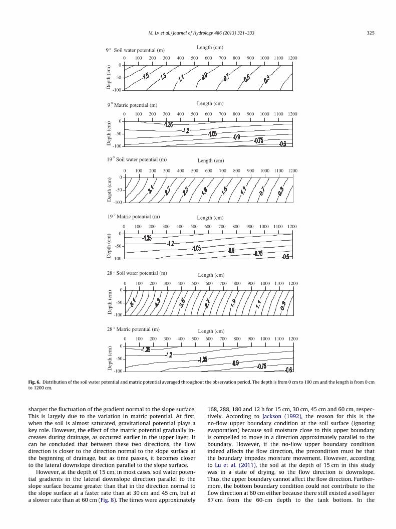
Based on Eqs. (3) and (4), the soil water potential of all the ob-served points can be obtained. Lu et al. (2011) noted that ‘‘it is thegradient of moisture content at the point of interest that controlsthe flow direction at that point.’’ However, in this study, the matricpotential (moisture content) was not found to completely controlthe flow direction, as shown in Fig. 6. To better understand the flowdirection in the longitudinal hillslope profile (i.e., the vertical pro-file in the length direction), contours of soil water potential andmatric potential were developed using the spatial interpolationmethod, i.e., the modified Shepard’s method (Yang et al., 2004).Unless specified otherwise, this method was used throughout thestudy. Fig. 6 presents contours of soil water potential and matricpotential for the experiments carried out at 9�, 19� and 28�. Thisfigure shows that the patterns are obviously different for the twopotentials. In Lu et al. (2011)’s study, the flow direction hypothesisexplained only by the matric potential between two arbitrarypoints is correct because those two points had the same elevationin their study. Thus, soil water potential was used to investigatethe flow direction in this study.

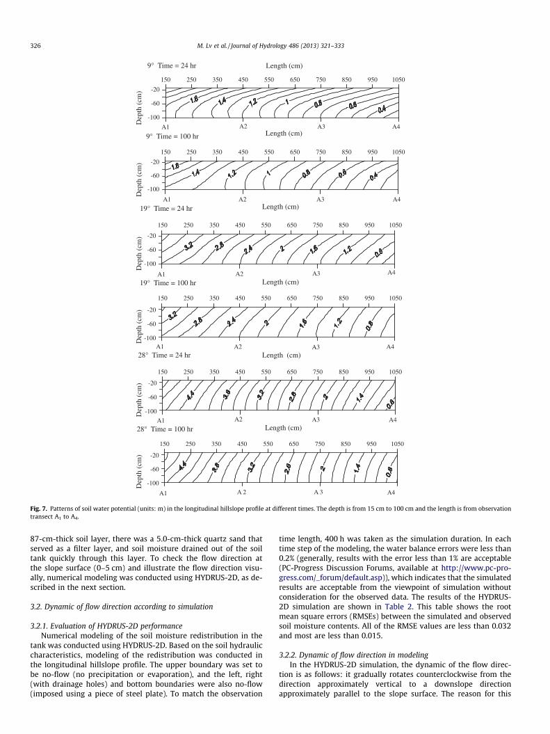
Flow directions in the longitudinal hillslope profile are shown inFig. 7. To avoid extension errors, the domain was interpolated from15 to 100 cm in depth and from A1 to A4 in slope length, ratherthan from 0 to 100 cm in depth and 0–1200 cm in slope length.As Fig. 7 shows, the flows were in the lateral downslope directionall over this hillslope profile during the drying phase, which is con-sistent with the results obtained by Lu et al. (2011). The potentialvertical gradients ow/oz were negative, which is consistent withthe conclusion of Sinai and Dirksen (2006). The deviation of theflow direction from the vertical at 100 cm is greater than in theupper soil layers, especially in the 9� experiment and at 24 h afterdrainage. After 100 h, the flow directions all over the profile aremuch similar. That is, lateral downslope flow approximately paral-lel to the slope surface first appears at the depth of 100 cm. Lu et al.(2011) showed that the lateral downslope flow direction is alwaysmost pronounced at the slope surface and is nearly parallel to theslope surface. In this study, because shallow soil depths (0–5 cm)were not monitored, the flow direction at the surface cannot bedetermined from the measured results. However, the flow direc-tion at 15 cm can be examined, as described next.

The concept of the soil water potential gradient (Dw/Dx, wherex represents a certain direction) is employed. The soil water poten-tial gradient is the ratio of the difference in soil water potential tothe distance in a certain direction between two points in the soil.For instance, (A2-15)–(A3-15) represents the ratio of potentialdifference and the lateral downslope straight-line distance be-tween A2 and A3 at the depth of 15 cm (i.e., 300 cm). Fig. 8 showscomparisons of soil water potential gradients between two direc-tions during the testing. One is the lateral downslope directionparallel to the slope surface (e.g., (A2-15)–(A3-15)) and the otheris the direction normal to the slope surface (e.g., (A2-15)–(A2-30)). Fig. 8 shows that the gradient of soil water potential normalto the slope surface fluctuates greatly, while the lateral gradienthardly fluctuates at all. In particular, the shallower the layer, the

0 100 200 300 400 500 600 700 800 900 1000 1100 1200

0 100 200 300 400 500 600 700 800 900 1000 1100 1200

0 100 200 300 400 500 600 700 800 900 1000 1100 1200

0 100 200 300 400 500 600 700 800 900 1000 1100 1200

0 100 200 300 400 500 600 700 800 900 1000 1100 1200

0 100 200 300 400 500 600 700 800 900 1000 1100 1200

Length (cm)

-100

-50

0

Dep

th (

cm)

9 Soil water potential (m)

Length (cm)

-100

-50

0

Dep

th (

cm)

9 Matric potential (m)

Length (cm)

-100

-50

0

Dep

th (

cm)

19 Soil water potential (m)

Length (cm)

-100

-50

0

Dep

th (

cm)

19 Matric potential (m)

Length (cm)

-100

-50

0

Dep

th (

cm)

28 Soil water potential (m)

Length (cm)

-100

-50

0

Dep

th (

cm)

28 Matric potential (m)

°

°

°

°

°

°

Fig. 6. Distribution of the soil water potential and matric potential averaged throughout the observation period. The depth is from 0 cm to 100 cm and the length is from 0 cmto 1200 cm.

M. Lv et al. / Journal of Hydrology 486 (2013) 321–333 325

sharper the fluctuation of the gradient normal to the slope surface.This is largely due to the variation in matric potential. At first,when the soil is almost saturated, gravitational potential plays akey role. However, the effect of the matric potential gradually in-creases during drainage, as occurred earlier in the upper layer. Itcan be concluded that between these two directions, the flowdirection is closer to the direction normal to the slope surface atthe beginning of drainage, but as time passes, it becomes closerto the lateral downslope direction parallel to the slope surface.

However, at the depth of 15 cm, in most cases, soil water poten-tial gradients in the lateral downslope direction parallel to theslope surface became greater than that in the direction normal tothe slope surface at a faster rate than at 30 cm and 45 cm, but ata slower rate than at 60 cm (Fig. 8). The times were approximately

168, 288, 180 and 12 h for 15 cm, 30 cm, 45 cm and 60 cm, respec-tively. According to Jackson (1992), the reason for this is theno-flow upper boundary condition at the soil surface (ignoringevaporation) because soil moisture close to this upper boundaryis compelled to move in a direction approximately parallel to theboundary. However, if the no-flow upper boundary conditionindeed affects the flow direction, the precondition must be thatthe boundary impedes moisture movement. However, accordingto Lu et al. (2011), the soil at the depth of 15 cm in this studywas in a state of drying, so the flow direction is downslope.Thus, the upper boundary cannot affect the flow direction. Further-more, the bottom boundary condition could not contribute to theflow direction at 60 cm either because there still existed a soil layer87 cm from the 60-cm depth to the tank bottom. In the

Length (cm)

-100

-60

-20

Dep

th (

cm)

19° Time = 24 hr

A1 A2 A3 A4

Length (cm)

-100

-60

-20

Dep

th (

cm)

19° Time = 100 hr

A1 A2 A3 A428° Time = 24 hr

28° Time = 100 hr

Length (cm)

-100

-60

-20

Dep

th (

cm)

9° Time = 100 hr

A1 A2 A3 A4

150 250 350 450 550 650 750 850 950 1050

150 250 350 450 550 650 750 850 950 1050

150 250 350 450 550 650 750 850 950 1050

150 250 350 450 550 650 750 850 950 1050

150 250 350 450 550 650 750 850 950 1050

150 250 350 450 550 650 750 850 950 1050

Length (cm)

-100

-60

-20

Dep

th (

cm)

A1 A2 A3 A4

9° Time = 24 hr

Length (cm)

-100

-60

-20

Dep

th (

cm)

A1 A2 A3 A4Length (cm)

-100

-60

-20

Dep

th (

cm)

A1 A 2 A 3 A4

Fig. 7. Patterns of soil water potential (units: m) in the longitudinal hillslope profile at different times. The depth is from 15 cm to 100 cm and the length is from observationtransect A1 to A4.

326 M. Lv et al. / Journal of Hydrology 486 (2013) 321–333

87-cm-thick soil layer, there was a 5.0-cm-thick quartz sand thatserved as a filter layer, and soil moisture drained out of the soiltank quickly through this layer. To check the flow direction atthe slope surface (0–5 cm) and illustrate the flow direction visu-ally, numerical modeling was conducted using HYDRUS-2D, as de-scribed in the next section.

3.2. Dynamic of flow direction according to simulation

3.2.1. Evaluation of HYDRUS-2D performanceNumerical modeling of the soil moisture redistribution in the

tank was conducted using HYDRUS-2D. Based on the soil hydrauliccharacteristics, modeling of the redistribution was conducted inthe longitudinal hillslope profile. The upper boundary was set tobe no-flow (no precipitation or evaporation), and the left, right(with drainage holes) and bottom boundaries were also no-flow(imposed using a piece of steel plate). To match the observation

time length, 400 h was taken as the simulation duration. In eachtime step of the modeling, the water balance errors were less than0.2% (generally, results with the error less than 1% are acceptable(PC-Progress Discussion Forums, available at http://www.pc-pro-gress.com/_forum/default.asp)), which indicates that the simulatedresults are acceptable from the viewpoint of simulation withoutconsideration for the observed data. The results of the HYDRUS-2D simulation are shown in Table 2. This table shows the rootmean square errors (RMSEs) between the simulated and observedsoil moisture contents. All of the RMSE values are less than 0.032and most are less than 0.015.

3.2.2. Dynamic of flow direction in modelingIn the HYDRUS-2D simulation, the dynamic of the flow direc-

tion is as follows: it gradually rotates counterclockwise from thedirection approximately vertical to a downslope directionapproximately parallel to the slope surface. The reason for this

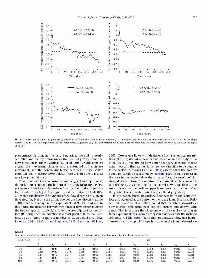
Fig. 8. Comparisons of soil water potential gradients in different directions of 19� experiment, i.e., lateral downslope parallel to the slope surface and normal to the slopesurface. ‘‘(A2-15)–(A3-15)’’ represents the soil water potential gradient (Dw/Dx) in the lateral downslope direction parallel to the slope surface between A2 and A3 at the depthof 15 cm.

M. Lv et al. / Journal of Hydrology 486 (2013) 321–333 327

phenomenon is that, at the very beginning, the soil is nearlysaturated and mainly drains under the force of gravity; thus theflow direction is almost vertical (Lu et al., 2011). With ongoingdrying, the movement changes into unsaturated soil moisturemovement, and the controlling factor becomes the soil waterpotential. Soil moisture always flows from a high-potential areato a low-potential area.

Consistent with the conclusions concerning soil water potential,the surface (0–5 cm) and the bottom of the sandy loam are the firstplaces to exhibit lateral downslope flow parallel to the slope sur-face, as shown in Fig. 9. The figure is a direct output of HYDRUS-2D, which can display the dynamic of the flow direction at a giventime step. Fig. 9 shows the distribution of the flow direction at the100th hour of drainage in the experiments at 9�, 19�, and 28�. Inthis figure, the distance between two lines of flow direction alongthe slope is approximately 5.0 cm. For the area adjacent to the sur-face (0–5 cm), the flow direction is almost parallel to the soil sur-face, as also found in quite a number of studies (Jackson, 1992;Lu et al., 2011; McCord and Stephens, 1987; Sinai and Dirksen,

Table 2Root mean square errors (RMSEs) between simulated and observed volumetric soil moistu

Depth (cm) 9� 19�

A1 A2 A3 A4 A1 A2

15 0.007 0.006 0.007 0.008 0.005 0.030 0.008 0.009 0.010 0.010 0.004 0.045 0.011 0.012 0.011 0.009 0.002 0.060 0.011 0.009 0.011 0.013 0.002 0.0

100 0.014 0.017 0.015 0.022 0.014 0.0

2006). Downslope flows with deviations from the vertical greaterthan (90� � a) do not appear in this paper or in the study of Luet al. (2011). Thus, the no-flow upper boundary does not impedewater flow and thus cannot force the flow direction to be parallelto the surface. Although Lu et al. (2011) asserted that the no-flowboundary condition identified by Jackson (1992) is only correct inthe area immediately below the slope surface, the results of thisstudy do not confirm this assertion. Therefore, it can be concludedthat the necessary condition for the lateral downslope flow at thesoil surface is not the no-flow upper boundary condition but ratherthe gradient of soil water potential (i.e., the drying state).

In this paper, lateral downslope flow parallel to the slope sur-face also occurred at the bottom of the sandy loam. Sinai and Dirk-sen (2006) and Lu et al. (2011) found that the lateral downslopeflow is most significant near the soil surface and decays withdepth. This is because the slope angle at the sandbox bottom intheir experiments was zero, so they could not examine the inclinedsoil bottom. Tóth (1963) found that groundwater flow in a homo-geneous and isotropic hillslope is always in the lateral downslope

re contents for different experiments.

28�

A3 A4 A1 A2 A3 A4

07 0.009 0.013 0.004 0.004 0.006 0.01304 0.007 0.016 0.006 0.004 0.006 0.01305 0.008 0.008 0.008 0.006 0.006 0.00807 0.007 0.017 0.009 0.008 0.007 0.01216 0.017 0.031 0.016 0.021 0.018 0.011

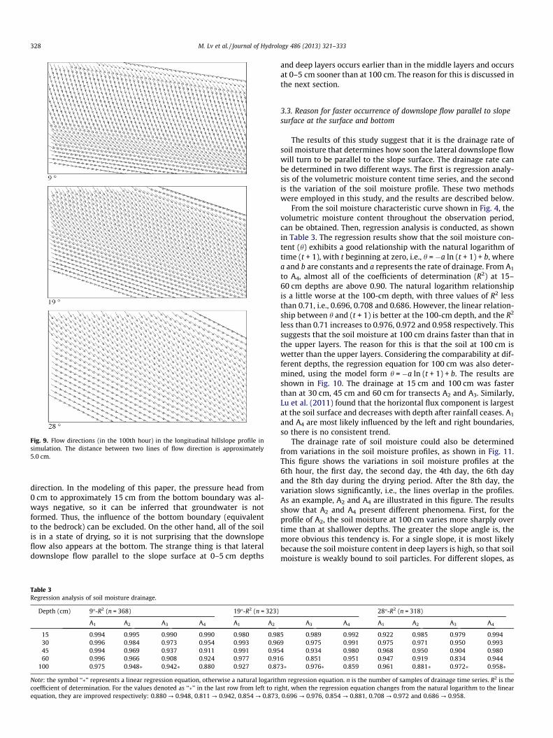
Fig. 9. Flow directions (in the 100th hour) in the longitudinal hillslope profile insimulation. The distance between two lines of flow direction is approximately5.0 cm.

328 M. Lv et al. / Journal of Hydrology 486 (2013) 321–333

direction. In the modeling of this paper, the pressure head from0 cm to approximately 15 cm from the bottom boundary was al-ways negative, so it can be inferred that groundwater is notformed. Thus, the influence of the bottom boundary (equivalentto the bedrock) can be excluded. On the other hand, all of the soilis in a state of drying, so it is not surprising that the downslopeflow also appears at the bottom. The strange thing is that lateraldownslope flow parallel to the slope surface at 0–5 cm depths

Table 3Regression analysis of soil moisture drainage.

Depth (cm) 9�-R2 (n = 368) 19�-R2 (n = 323)

A1 A2 A3 A4 A1 A2

15 0.994 0.995 0.990 0.990 0.980 0.9830 0.996 0.984 0.973 0.954 0.993 0.9645 0.994 0.969 0.937 0.911 0.991 0.9560 0.996 0.966 0.908 0.924 0.977 0.91

100 0.975 0.948� 0.942� 0.880 0.927 0.87

Note: the symbol ‘‘�’’ represents a linear regression equation, otherwise a natural logarithcoefficient of determination. For the values denoted as ‘‘�’’ in the last row from left to riequation, they are improved respectively: 0.880 ? 0.948, 0.811 ? 0.942, 0.854 ? 0.873

and deep layers occurs earlier than in the middle layers and occursat 0–5 cm sooner than at 100 cm. The reason for this is discussed inthe next section.

3.3. Reason for faster occurrence of downslope flow parallel to slopesurface at the surface and bottom

The results of this study suggest that it is the drainage rate ofsoil moisture that determines how soon the lateral downslope flowwill turn to be parallel to the slope surface. The drainage rate canbe determined in two different ways. The first is regression analy-sis of the volumetric moisture content time series, and the secondis the variation of the soil moisture profile. These two methodswere employed in this study, and the results are described below.

From the soil moisture characteristic curve shown in Fig. 4, thevolumetric moisture content throughout the observation period,can be obtained. Then, regression analysis is conducted, as shownin Table 3. The regression results show that the soil moisture con-tent (h) exhibits a good relationship with the natural logarithm oftime (t + 1), with t beginning at zero, i.e., h = �a ln (t + 1) + b, wherea and b are constants and a represents the rate of drainage. From A1

to A4, almost all of the coefficients of determination (R2) at 15–60 cm depths are above 0.90. The natural logarithm relationshipis a little worse at the 100-cm depth, with three values of R2 lessthan 0.71, i.e., 0.696, 0.708 and 0.686. However, the linear relation-ship between h and (t + 1) is better at the 100-cm depth, and the R2

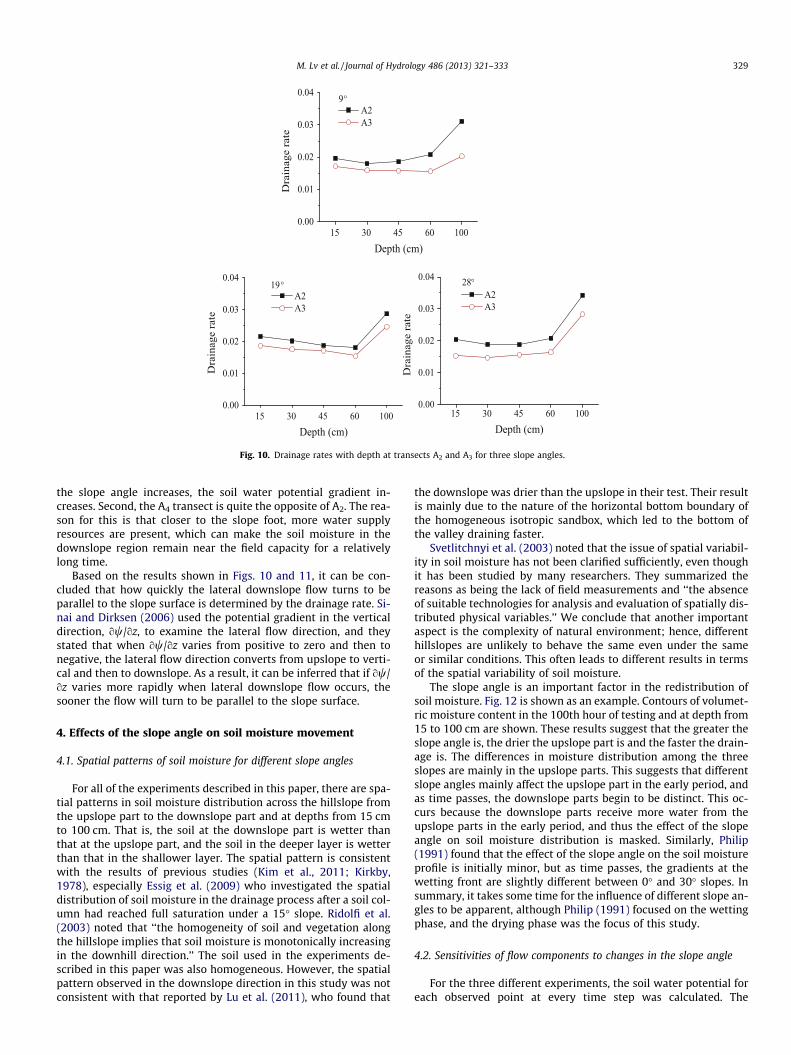
less than 0.71 increases to 0.976, 0.972 and 0.958 respectively. Thissuggests that the soil moisture at 100 cm drains faster than that inthe upper layers. The reason for this is that the soil at 100 cm iswetter than the upper layers. Considering the comparability at dif-ferent depths, the regression equation for 100 cm was also deter-mined, using the model form h = �a ln (t + 1) + b. The results areshown in Fig. 10. The drainage at 15 cm and 100 cm was fasterthan at 30 cm, 45 cm and 60 cm for transects A2 and A3. Similarly,Lu et al. (2011) found that the horizontal flux component is largestat the soil surface and decreases with depth after rainfall ceases. A1

and A4 are most likely influenced by the left and right boundaries,so there is no consistent trend.

The drainage rate of soil moisture could also be determinedfrom variations in the soil moisture profiles, as shown in Fig. 11.This figure shows the variations in soil moisture profiles at the6th hour, the first day, the second day, the 4th day, the 6th dayand the 8th day during the drying period. After the 8th day, thevariation slows significantly, i.e., the lines overlap in the profiles.As an example, A2 and A4 are illustrated in this figure. The resultsshow that A2 and A4 present different phenomena. First, for theprofile of A2, the soil moisture at 100 cm varies more sharply overtime than at shallower depths. The greater the slope angle is, themore obvious this tendency is. For a single slope, it is most likelybecause the soil moisture content in deep layers is high, so that soilmoisture is weakly bound to soil particles. For different slopes, as

28�-R2 (n = 318)

A3 A4 A1 A2 A3 A4

5 0.989 0.992 0.922 0.985 0.979 0.9949 0.975 0.991 0.975 0.971 0.950 0.9934 0.934 0.980 0.968 0.950 0.904 0.9806 0.851 0.951 0.947 0.919 0.834 0.9443� 0.976� 0.859 0.961 0.881� 0.972� 0.958�

m regression equation. n is the number of samples of drainage time series. R2 is theght, when the regression equation changes from the natural logarithm to the linear, 0.696 ? 0.976, 0.854 ? 0.881, 0.708 ? 0.972 and 0.686 ? 0.958.

°

°°

Fig. 10. Drainage rates with depth at transects A2 and A3 for three slope angles.

M. Lv et al. / Journal of Hydrology 486 (2013) 321–333 329

the slope angle increases, the soil water potential gradient in-creases. Second, the A4 transect is quite the opposite of A2. The rea-son for this is that closer to the slope foot, more water supplyresources are present, which can make the soil moisture in thedownslope region remain near the field capacity for a relativelylong time.

Based on the results shown in Figs. 10 and 11, it can be con-cluded that how quickly the lateral downslope flow turns to beparallel to the slope surface is determined by the drainage rate. Si-nai and Dirksen (2006) used the potential gradient in the verticaldirection, ow/oz, to examine the lateral flow direction, and theystated that when ow/oz varies from positive to zero and then tonegative, the lateral flow direction converts from upslope to verti-cal and then to downslope. As a result, it can be inferred that if ow/oz varies more rapidly when lateral downslope flow occurs, thesooner the flow will turn to be parallel to the slope surface.

4. Effects of the slope angle on soil moisture movement

4.1. Spatial patterns of soil moisture for different slope angles

For all of the experiments described in this paper, there are spa-tial patterns in soil moisture distribution across the hillslope fromthe upslope part to the downslope part and at depths from 15 cmto 100 cm. That is, the soil at the downslope part is wetter thanthat at the upslope part, and the soil in the deeper layer is wetterthan that in the shallower layer. The spatial pattern is consistentwith the results of previous studies (Kim et al., 2011; Kirkby,1978), especially Essig et al. (2009) who investigated the spatialdistribution of soil moisture in the drainage process after a soil col-umn had reached full saturation under a 15� slope. Ridolfi et al.(2003) noted that ‘‘the homogeneity of soil and vegetation alongthe hillslope implies that soil moisture is monotonically increasingin the downhill direction.’’ The soil used in the experiments de-scribed in this paper was also homogeneous. However, the spatialpattern observed in the downslope direction in this study was notconsistent with that reported by Lu et al. (2011), who found that

the downslope was drier than the upslope in their test. Their resultis mainly due to the nature of the horizontal bottom boundary ofthe homogeneous isotropic sandbox, which led to the bottom ofthe valley draining faster.

Svetlitchnyi et al. (2003) noted that the issue of spatial variabil-ity in soil moisture has not been clarified sufficiently, even thoughit has been studied by many researchers. They summarized thereasons as being the lack of field measurements and ‘‘the absenceof suitable technologies for analysis and evaluation of spatially dis-tributed physical variables.’’ We conclude that another importantaspect is the complexity of natural environment; hence, differenthillslopes are unlikely to behave the same even under the sameor similar conditions. This often leads to different results in termsof the spatial variability of soil moisture.

The slope angle is an important factor in the redistribution ofsoil moisture. Fig. 12 is shown as an example. Contours of volumet-ric moisture content in the 100th hour of testing and at depth from15 to 100 cm are shown. These results suggest that the greater theslope angle is, the drier the upslope part is and the faster the drain-age is. The differences in moisture distribution among the threeslopes are mainly in the upslope parts. This suggests that differentslope angles mainly affect the upslope part in the early period, andas time passes, the downslope parts begin to be distinct. This oc-curs because the downslope parts receive more water from theupslope parts in the early period, and thus the effect of the slopeangle on soil moisture distribution is masked. Similarly, Philip(1991) found that the effect of the slope angle on the soil moistureprofile is initially minor, but as time passes, the gradients at thewetting front are slightly different between 0� and 30� slopes. Insummary, it takes some time for the influence of different slope an-gles to be apparent, although Philip (1991) focused on the wettingphase, and the drying phase was the focus of this study.

4.2. Sensitivities of flow components to changes in the slope angle

For the three different experiments, the soil water potential foreach observed point at every time step was calculated. The

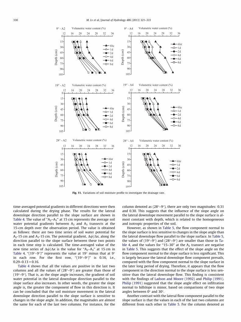
Fig. 11. Variations of soil moisture profile to investigate the drainage rate.

330 M. Lv et al. / Journal of Hydrology 486 (2013) 321–333

time-averaged potential gradients in different directions were thencalculated during the drying phase. The results for the lateraldownslope direction parallel to the slope surface are shown inTable 4. The value of ‘‘A2–A3’’ at 15 cm represents the average soilwater potential gradients between A2 and A3 transects at the15-cm depth over the observation period. The value is obtainedas follows: there are two time series of soil water potential forA2-15 cm and A3-15 cm. The potential gradient, Dw/Dx, along thedirection parallel to the slope surface between these two pointsin each time step is calculated. The time-averaged value of thenew time series of Dw/Dx is the value for ‘‘A2–A3’’ at 15 cm inTable 4. ‘‘(19�–9�)’’ represents the value at 19� minus that at 9�in each row. For the first row, ‘‘(19�–9�)’’ is 0.16, i.e.,0.29–0.13 = 0.16.

Table 4 shows that all the values are positive in the last twocolumns and all the values of (28�–9�) are greater than those of(19�–9�). That is, as the slope angle increases, the gradient of soilwater potential in the lateral downslope direction parallel to theslope surface also increases. In other words, the greater the slopeangle is, the greater the component of flow in this direction is. Itcan be concluded that the soil moisture movement in the lateraldownslope direction parallel to the slope surface is sensitive tochanges in the slope angle. In addition, the magnitudes are almostthe same for each of the last two columns. For instance, for the

column denoted as (28�–9�), there are only two magnitudes: 0.31and 0.30. This suggests that the influence of the slope angle onthe lateral downslope movement parallel to the slope surface is al-most constant with depth, which is related to the homogeneousand isotropic properties of the soil.

However, as shown in Table 5, the flow component normal tothe slope surface is less sensitive to changes in the slope angle thanthe lateral downslope flow parallel to the slope surface. In Table 5,the values of (19�–9�) and (28�–9�) are smaller than those in Ta-ble 4, and the values for ‘‘15–30’’ at the A2 transect are negativein Table 5. This suggests that the effect of the slope angle on theflow component normal to the slope surface is less significant. Thisis largely because the lateral downslope flow component prevails,compared with the flow component normal to the slope surface inthe later long period of drying. Therefore, it appears that the flowcomponent in the direction normal to the slope surface is less sen-sitive than the lateral downslope flow. This finding is consistentwith the findings of Ladson and Moore (1992) and Philip (1991).Philip (1991) suggested that the slope angle effect on infiltrationnormal to hillslope is minor, based on comparisons of two slopeangles between 0� and 30�.

Another contrast with the lateral flow component parallel to theslope surface is that the values in each of the last two columns aredifferent from each other in Table 5. For the column denoted as

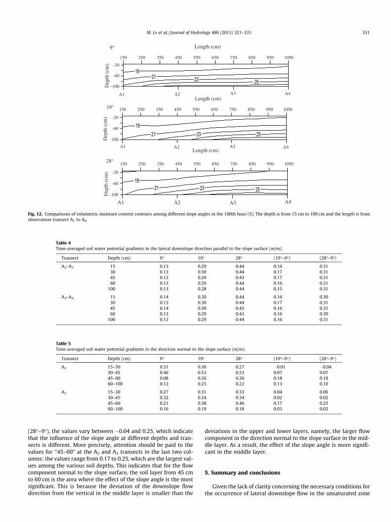
Table 4Time-averaged soil water potential gradients in the lateral downslope direction parallel to the slope surface (m/m).

Transect Depth (cm) 9� 19� 28� (19�–9�) (28�–9�)

A2–A3 15 0.13 0.29 0.44 0.16 0.3130 0.13 0.30 0.44 0.17 0.3145 0.12 0.29 0.43 0.17 0.3160 0.13 0.29 0.44 0.16 0.31

100 0.13 0.28 0.44 0.15 0.31

A3–A4 15 0.14 0.30 0.44 0.16 0.3030 0.13 0.30 0.44 0.17 0.3145 0.14 0.30 0.45 0.16 0.3160 0.13 0.29 0.43 0.16 0.30

100 0.13 0.29 0.44 0.16 0.31

Table 5Time-averaged soil water potential gradients in the direction normal to the slope surface (m/m).

Transect Depth (cm) 9� 19� 28� (19�–9�) (28�–9�)

A2 15–30 0.31 0.30 0.27 �0.01 �0.0430–45 0.46 0.53 0.53 0.07 0.0745–60 0.08 0.26 0.26 0.18 0.1860–100 0.12 0.25 0.22 0.13 0.10

A3 15–30 0.27 0.31 0.33 0.04 0.0630–45 0.32 0.34 0.34 0.02 0.0245–60 0.21 0.38 0.46 0.17 0.2560–100 0.16 0.19 0.18 0.03 0.02

150 250 350 450 550 650 750 850 950 1050

150 250 350 450 550 650 750 850 950 1050

150 250 350 450 550 650 750 850 950 1050

Length (cm)

-100

-60

-20

Dep

th (

cm)

9°

Length (cm)

-100

-60

-20

Dep

th (

cm)

19°

Length (cm)

-100

-60

-20

Dep

th (

cm)

28°

A1 A2 A3 A4

A2 A3 A4

A1

A1

A2 A3 A4

Fig. 12. Comparisons of volumetric moisture content contours among different slope angles in the 100th hour (%). The depth is from 15 cm to 100 cm and the length is fromobservation transect A1 to A4.

M. Lv et al. / Journal of Hydrology 486 (2013) 321–333 331

(28�–9�), the values vary between �0.04 and 0.25, which indicatethat the influence of the slope angle at different depths and tran-sects is different. More precisely, attention should be paid to thevalues for ‘‘45–60’’ at the A2 and A3 transects in the last two col-umns: the values range from 0.17 to 0.25, which are the largest val-ues among the various soil depths. This indicates that for the flowcomponent normal to the slope surface, the soil layer from 45 cmto 60 cm is the area where the effect of the slope angle is the mostsignificant. This is because the deviation of the downslope flowdirection from the vertical in the middle layer is smaller than the

deviations in the upper and lower layers, namely, the larger flowcomponent in the direction normal to the slope surface in the mid-dle layer. As a result, the effect of the slope angle is more signifi-cant in the middle layer.

5. Summary and conclusions

Given the lack of clarity concerning the necessary conditions forthe occurrence of lateral downslope flow in the unsaturated zone

332 M. Lv et al. / Journal of Hydrology 486 (2013) 321–333

and the effects of different slope angles on soil moisture move-ment, laboratory experiments of soil moisture distribution werecarried out using a large variable-slope soil tank. In addition,numerical modeling was conducted using HYDRUS-2D. The con-clusions are as follows:

The flow direction of soil moisture gradually rotates counter-clockwise from the vertical direction to the lateral downslopedirection parallel to the slope surface. Lateral downslope flow par-allel to the slope surface first appeared at the surface (0–5 cm) andat the bottom of the sandy loam used in the experiments. The for-mation of lateral downslope flow parallel to the slope surface atthe surface is due to the state of drying rather than the no-flowupper boundary condition, which is consistent with the conclusionreached by Lu et al. (2011) rather than with that reached by Jack-son (1992). In this study, the upper boundary was not found to im-pede soil moisture movement at the surface. At the bottom, lateraldownslope flow also occurs due to the state of drying rather thanthe bottom boundary. The drainage rate dictates the rate at whichlateral downslope flow turns to be parallel to the slope surface,which has not been reported previously. In the surface and bottomareas, drainage was faster than in the middle layers. Specifically, atthe depth of 0–5 cm, lateral flow parallel to the slope surface oc-curred earlier than at the depth of 100 cm, while flow at the depthof 15 cm occurred later than at the depth of 100 cm. The formationof lateral downslope flow is due to the state of drying, but the rateat which lateral downslope flow turns to be parallel to the slopesurface is due to the drainage rate. The results of this study alsoshow that the flow component in the lateral downslope directionparallel to the slope surface is more sensitive to changes in theslope angle than is the flow component normal to the slope sur-face. The influence of the slope angle on the flow component nor-mal to the slope surface is greatest in the middle layer.

[38] Based on the drainage rate of soil moisture in the dryingphase, it can be conjectured which soil layer is the most likely toexhibit lateral downslope unsaturated flow parallel to the slopesurface. The results of this study may have some significance forcontaminant transport. For other soil types, the spatial patternsof soil moisture distribution would most likely be similar to thesandy loam investigated in this paper, but the rates of drainagewould be different because of the different specific retentionsand specific yields of different soils. Many factors contribute to soilmoisture variation. In this study, only water-routing processes un-der slope angles were isolated and considered. If several other fac-tors of influence were also taken into account, the situation wouldbe more complicated, and the results may be different from thoseobtained in this study. It may be worthwhile to conduct experi-ments to examine the multiple factors that influence soil moisturevariation, along with different soil types and more diverse slopeangles.

Acknowledgements

This research was supported by National Natural Science Foun-dation of China (Grant Nos. 41101015, 40830639 and 50879016),the National Basic Research Program of China (Grant No.2010CB951101) and the Special Fund of State Key Laboratory ofHydrology-Water Resources and Hydraulic Engineering (1069-50985512). We appreciate anonymous reviewers, whose com-ments and ideas improved the original manuscript.

References

Beven, K., Kirkby, M., 1979. A physically based variable contributing area model ofbasin hydrology. Hydrol. Sci. J. 24 (1), 43–69.

Bronstert, A., 1999. Capabilities and limitations of detailed hillslope hydrologicalmodelling. Hydrol. Process. 13 (1), 21–48.

Essig, E.T., Corradini, C., Morbidelli, R., Govindaraju, R.S., 2009. Infiltration and deepflow over sloping surfaces: comparison of numerical and experimental results. J.Hydrol. 374 (1), 30–42. http://dx.doi.org/10.1016/j.jhydrol.2009.05.017.

Genereux, D.P., Hemond, H.F., 1990. Naturally occurring radon 222 as a tracer forstreamflow generation: steady state methodology and field example. WaterResour. Res. 26 (12), 3065–3075. http://dx.doi.org/10.1029/WR026i012p03065.

Grayson, R.B., Western, A.W., Chiew, F.H.S., Blöschl, G., 1997. Preferred states inspatial soil moisture patterns: local and nonlocal controls. Water Resour. Res.33 (12), 2897–2908.

Hopp, L., McDonnell, J.J., 2009. Connectivity at the hillslope scale: identifyinginteractions between storm size, bedrock permeability, slope angle and soildepth. J. Hydrol. 376 (3–4), 378–391. http://dx.doi.org/10.1016/j.jhydrol.2009.07.047.

Islam, N., Wallender, W., Mitchell, J., Wicks, S., Howitt, R., 2006. Performanceevaluation of methods for the estimation of soil hydraulic parameters and theirsuitability in a hydrologic model. Geoderma 134 (1–2), 135–151. http://dx.doi.org/10.1016/j.geoderma.2005.09.004.

Jackson, C.R., 1992. Hillslope infiltration and lateral downslope unsaturated flow.Water Resour. Res. 28 (9), 2533–2539.

Jawson, S.D., Niemann, J.D., 2007. Spatial patterns from EOF analysis of soil moistureat a large scale and their dependence on soil, land-use, and topographicproperties. Adv. Water Resour. 30 (3), 366–381. http://dx.doi.org/10.1016/j.advwatres.2006.05.006.

Kandelous, M., Šimunek, J., 2010. Numerical simulations of water movement in asubsurface drip irrigation system under field and laboratory conditions usingHYDRUS-2D. Agric. Water Manage. 97 (7), 1070–1076. http://dx.doi.org/10.1016/j.agwat.2010.02.012.

Kim, H.J., Sidle, R.C., Moore, R.D., 2005. Shallow lateral flow from a forestedhillslope: influence of antecedent wetness. Catena 60 (3), 293–306. http://dx.doi.org/10.1016/j.catena.2004.12.005.

Kim, S., 2009. Multivariate analysis of soil moisture history for a hillslope. J. Hydrol.374 (3–4), 318–328. http://dx.doi.org/10.1016/j.jhydrol.2009.06.025.

Kim, S., Kim, H., 2007. Stochastic analysis of soil moisture to understand spatial andtemporal variations of soil wetness at a steep hillside. J. Hydrol. 341, 1–11.http://dx.doi.org/10.1016/j.jhydrol.2007.04.012.

Kim, S., Sun, H., Jung, S., 2011. Configuration of the relationship of soil moistures forvertical soil profiles on a steep hillslope using a vector time series model. J.Hydrol. 399 (3–4), 353–363. http://dx.doi.org/10.1016/j.jhydrol.2011.01.012.

Kirkby, M., 1978. Hillslope Hydrology. Wiley Chichester.Ladson, A., Moore, I., 1992. Soil water prediction on the Konza Prairie by

microwave remote sensing and topographic attributes. J. Hydrol. 138 (3–4),385–407.

Lu, N., Kaya, B.S., Godt, J.W., 2011. Direction of unsaturated flow in a homogeneousand isotropic hillslope. Water Resour. Res. 47, W02519. http://dx.doi.org/10.1029/2010WR010003.

Lv, H., Zhu, Y., Skaggs, T., Yu, Z., 2009. Comparison of measured and simulated waterstorage in dryland terraces of the Loess Plateau, China. Agric. Water Manage. 96(2), 299–306. http://dx.doi.org/10.1016/j.agwat.2008.08.010.

McCord, J., Stephens, D., 1987. Lateral moisture flow beneath a sandy hillslopewithout an apparent impeding layer. Hydrol. Process. 1 (3), 225–238.

McCord, J.T., Stephens, D.B., Wilson, J.L., 1991. Hysteresis and state-dependentanisotropy in modeling unsaturated hillslope hydrologic processes. WaterResour. Res. 27 (7), 1501–1518.

Miyazaki, T., 1988. Water flow in unsaturated soil in layered slopes. J. Hydrol. 102(1–4), 201–214.

Moore, I.D., Norton, T., Williams, J.E., 1993. Modelling environmental heterogeneityin forested landscapes. J. Hydrol. 150 (2–4), 717–747. http://dx.doi.org/10.1016/0022-1694(93)90133-T.

Morbidelli, R., Corradini, C., Saltalippi, C., Govindaraju, R.S., 2008. Laboratoryexperimental investigation of infiltration by the run-on process. ASCE J. Hydrol.Eng. 13 (12), 1187–1192. http://dx.doi.org/10.1061/(ASCE)1084-0699(2008)13:12(1187.

Pan, L., Warrick, A., Wierenga, P., 1997. Downward water flow through slopinglayers in the vadose zone: time-dependence and effect of slope length. J. Hydrol.199 (1), 36–52.

Pat, J.F.Y., Eltahir, E.A.B., 1998. Stochastic analysis of the relationship betweentopography and the spatial distribution of soil moisture. Water Resour. Res. 34(5), 1251–1263.

Penna, D., Borga, M., Norbiato, D., Dalla Fontana, G., 2009. Hillslope scale soilmoisture variability in a steep alpine terrain. J. Hydrol. 364 (3–4), 311–327.http://dx.doi.org/10.1016/j.jhydrol.2008.11.009.

Perry, M.A., Niemann, J.D., 2007. Analysis and estimation of soil moisture at thecatchment scale using EOFs. J. Hydrol. 334 (3–4), 388–404. http://dx.doi.org/10.1016/j.jhydrol.2006.10.014.

Philip, J.R., 1991. Hillslope infiltration: planar slopes. Water Resour. Res. 27 (1),109–117.

Ridolfi, L., D’Odorico, P., Porporato, A., Rodriguez-Iturbe, I., 2003. Stochastic soilmoisture dynamics along a hillslope. J. Hydrol. 272 (1–4), 264–275. http://dx.doi.org/10.1016/s0022-1694(02)00270-6.

Šimunek, J., Šejna, M. and Van Genuchten, M., 1999. The HYDRUS-2D softwarepackage for simulating two-dimensional movement of water, heat, andmultiple solutes in variably saturated media. Version 2.0. US SalinityLaboratory, Riverside, CA.

Sinai, G., Dirksen, C., 2006. Experimental evidence of lateral flow in unsaturatedhomogeneous isotropic sloping soil due to rainfall. Water Resour. Res. 42,W12402. http://dx.doi.org/10.1029/2005WR004617.

M. Lv et al. / Journal of Hydrology 486 (2013) 321–333 333

Sloan, P.G., Moore, I.D., 1984. Modeling subsurface stormflow on steeply slopingforested watersheds. Water Resour. Res. 20 (12), 1815–1822.

Svetlitchnyi, A., Plotnitskiy, S., Stepovaya, O., 2003. Spatial distribution of soilmoisture content within catchments and its modelling on the basis oftopographic data. J. Hydrol. 277 (1–2), 50–60. http://dx.doi.org/10.1016/S0022-1694(03)00083-0.

Tromp-van Meerveld, H.J., McDonnell, J.J., 2006. On the interrelations betweentopography, soil depth, soil moisture, transpiration rates and speciesdistribution at the hillslope scale. Adv. Water Resour. 29 (2), 293–310. http://dx.doi.org/10.1016/j.advwatres.2005.02.016.

Tóth, J., 1963. A theoretical analysis of groundwater flow in small drainage basins. J.Geophys. Res. 68 (16), 4795–4812.

Van Genuchten, M.T., 1980. A closed-form equation for predicting the hydraulicconductivity of unsaturated soils. Soil Sci. Soc. Am. J. 44 (5), 892–898.

Warrick, A., Wierenga, P., Pan, L., 1997. Downward water flow through slopinglayers in the vadose zone: analytical solutions for diversions. J. Hydrol. 192 (1),321–337.

Western, A., Grayson, R., 1998. The Tarrawarra data set: soil moisture patterns, soilcharacteristics, and hydrological flux measurements. Water Resour. Res. 34(10), 2765–2768.

Wilson, D.J., Western, A.W., Grayson, R.B., 2005. A terrain and data-based methodfor generating the spatial distribution of soil moisture. Adv. Water Resour. 28(1), 43–54. http://dx.doi.org/10.1016/j.advwatres.2004.09.007.

Yang, C.S., Kao, S.P., Lee, F.B., Hung, P.S., 2004. Twelve different interpolationmethods: a case study of Surfer 8.0. Proceedings of the XXth ISPRS Congress.Istanbul. Turkey, pp. 778–785.

Yoo, C., Kim, S., 2004. EOF analysis of surface soil moisture field variability. Adv.Water Resour. 27 (8), 831–842. http://dx.doi.org/10.1016/j.advwatres.2004.04.003.

Zaslavsky, D., Sinai, G., 1981. Surface hydrology: I. Explanation of phenomena. J.Hydraul. Div. 107 (1), 1–16.

Zhao, S., Liu, J., Yang, G., Huo, L., Qian, T., 2008. Impact of particle size on soilmoisture characteristic curve. J. Taiyuan Univ. Sci. Technol. 29, 332–334 (inChinese).