concentration indicators: assessing the gap between ... · concentration indicators: assessing the...

Concentration indicators: Assessing the gap between aggregate and detailed data 1

Concentration indicators:

Assessing the gap between aggregate and detailed data

Fernando Ávila1, Emilio Flores1, Fabrizio López-Gallo1,2, and Javier Márquez3

Abstract

Risk analysis depends to a large extent on the type of data. Aggregate data can serve as a useful surrogate for individual data. However, in practice, there is uncertainty on the reliability and adequacy of aggregated data. In this paper we estimate the Herfindahl-Hirschman Index (HHI) for a loan portfolio using both aggregate data and individual data. Then, we compare both estimates to assess the reliability of the aggregated data. Concentration is a key driver of a portfolio credit risk and the HHI is a reliable standard for measuring concentration risk. Results for the Mexican banking system suggest that the estimated HHI based on aggregate data is a fairly good proxy for the actual concentration. This result suggests that aggregate data are useful to evaluate the underlying risk of the portfolio for regulatory purposes.

Keywords: Credit risk, Concentration risk, HHI index Data adequacy.

JEL Classification: C13, C18, G21, G32.

Introduction

Banks and other financial intermediaries tend to specialize in market segments where they exercise a competitive advantage. Whereas specialization facilitates banks to benefit from market conditions or their expertise, specialization may be accompanied by concentration of resources in counterparties, regions, industry sectors, or business products, compromising banks’ diversification of their sources of business or income. This lack of diversification increases a bank’s exposure to losses arising from the concentrated portfolio. Therefore, Concentration could work as a magnifying mechanism of financial shocks which may lead an institution to insolvency In fact, the Basel Committee on Banking Supervision (2006) affirms that “concentration is arguably the most important cause of large losses on banks’ portfolios”. The BCBS exhorts financial authorities to supervise and measure the risks of the portfolios of their financial institutions, including concentration risk.

The BCBS made an important effort at the beginning of the last decade to establish risk sensitive capital requirements for credit risk under Pillar I. It included a proposal to recognize concentration risk in a consistent manner. The main idea was to incorporate a Granularity Adjustment to the Asymptotic Single Risk Factor Model (ASRF) which is the base model for the IRB approach to compute capital requirements for credit risk. The ASRF computes the

1 Financial Stability Division at Banco de México. 2 Corresponding autor: [email protected] 3 Banorte

2

asymptotic loss distribution of loans portfolios, which is based on the model proposed by Vasicek (1987). The ASFR assumes that all credits in the portfolios are of equal size, and hence, credit VaR is asymptotically a linear function of the exposures in the portfolio. Evidently, real portfolios are not perfectly granular, so Gordy (2002) proposed to add a Granularity Adjustment factor to the ASRF, to include the diversification effect in the credit risk capital requirements of Basel II. Many authors further explore this approach: Gürtler et al. (2009), Bonollo et al. (2009), Lütkebohmert (2009), and Ebert and Lütkerbohmert (2010).

However, as Pillar I capital requirements for credit risk were intended to be derived from individual positions, the granularity adjustment introduced to capture concentration risk, dependent on the characteristics of the whole portfolio, was not compatible with the way overall capital requirements were computed. Indeed, credit risk capital requirements are obtained as the sum of the capital requirements applied to each exposure within the portfolio (see BCBS (2006b)).

As concentration risk, which is portfolio-based, is not yet considered under pillar I, Basel II permits additional capital requirements under Pillar II, subject to the discretion of local authorities. Pillar II explicitly states that regional authorities as well as banking institutions themselves “should supervise, measure, and control concentration risk in their credit portfolios” (see BCBS (2006), paragraph 773). To accomplish this task, banking supervisors and authorities should have their own models or estimates to monitor and measure the risk of banks’ portfolios. Hence, models used by supervisors should be sensitive to concentration, either implicitly or explicitly.

To include concentration risk, supervisors may need information on the full set of exposures of banks. This information is rarely available for supervisors around the world, especially for those of financial systems with a large number of banks where reporting the whole portfolios to the authorities may be complicated. Such supervisors may be provided only with information of the largest counterparties of the banks, but not with the full detail of small credits in the banks’ portfolios, and thus, risks may be neglected. Even if small credits may not contribute individually in a large extent to the bank’s risks, these credits may be generating concentrations in a single sector, such as small and medium size enterprises (SMEs), consumer loans and credit cards, or mortgages.

However supervisors may not need the full set of exposures of the banks: estimates of concentration may be enough. If, as in the case given above, supervisors are provided with aggregate information on the exposures of a bank, they will be able to compute estimates of the concentration, and then, additional capital requirements.

Few studies in the literature have proposed measures of concentration. The most popular ones have been the Herfindahl-Hirschman Index (HHI) and the Gini-Coefficient (GC is an inequality measure rather than a concentration one). Most of these measures where proposed to study industry concentration and market competition during the 70’s and 80’s4. At the end of the 80’s and during the 90’s, some of these measures were extended to measure concentration risk on portfolios.

Some methodologies to estimate concentration measures from aggregate data have been proposed in the literature. The main purpose of this paper is to review some of these methodologies and to assess their accuracy. To this end, information on the overall credit exposures of banks operating in Mexico is considered. This information is provided periodically by financial institutions to Mexican authorities and banking supervisors since the middle of the last decade. Before that, financial authorities and supervisors were only provided with information on the largest credits of each banks’ portfolios. Loans below a given threshold (200 thousand pesos or approximately 15 thousand US dollars) were

4 See Jacquemin and Berry (1979) and Clarke and Davis (1983).


aggregated in sector-buckets, and only the total amount of the bucket was reported: not even the number of credits in the bucket was known by supervisors. Thus, using the overall credit exposures of the banks, the exact concentration measures can be computed and compared to the estimates furnished by approximation methodologies, assuming that small-size loans are aggregated and only limited information is available.

The article proceeds as follows. Section 1 reviews some of the most popular measures of concentration proposed in the literature. From data on the portfolios of corporate loans and mortgages of banks operating in Mexico, these measures are estimated. Section 2 reviews some methodologies to estimate concentration measures, especially the HHI, when aggregate data is furnished. These methodologies are applied to the portfolios considered in section 1. Section 3 concludes.

1. Review of Concentration and Inequality Measures proposed in the literature

Concentration and Inequality are related concepts which have been historically confused. In a credit portfolio context, inequality refers to the distribution of the loans’ exposures within a portfolio, while concentration is related to the value of the portfolio which is held by a small number of debtors, as defined by Hoffman (1984). Both concepts are related as concentration incorporates both the size inequality of the exposures and the number of loans within the portfolio5,6.

The most common measure of concentration has historically been the Herfindhal-Hirschman Index (HHI), which is defined as:

∑=

=n

iiHHI

1

2ξ

1

where n is the number of credits in the portfolio and ξi is the exposure of credit i relative to the portfolio’s total value. Meanwhile, the most popular measure of inequality has been the Concentration Ratio (CR) defined as the aggregate share of the k-largest credits on the portfolio:

∑−

=−=

1

0)(

k

iin

kCR ξ

2

where ξ(1),… , ξ(n) are the relative exposures of the credits ordered from the smallest to the largest.

Hall and Tideman (1967) compare estimates of concentration from both measures and found that they produce similar results. However, they remarked that, even if the CR may be a good proxy for concentration and inequality, it has the main issue that it depends only on the k largest firms, neglecting the contribution of the smaller credits, and hence, changing k changes the accuracy of the CR. Moreover, given that when k→n the CR tends to 1, the value of k which provides more information should be estimated; but there is not a universal optimal value of k, because it depends on the structure of the portfolio.

5 See Bajo and Salas (1999). 6 In the case of concentration risk in credit portfolios, regulators should monitor concentration rather than

inequality. Actually, as will be shown later, there may be banks with highly unequal portfolios but well diversified, for example a bank which allocates a few credits to large size enterprises but a large number of loans to small debtors may have low concentration but high inequality.

4

A solution was given by the Gini-Coefficient (GC) which is the area between the Lorenz Curve7 of the portfolio and the Lorenz Curve of a perfectly diversified portfolio, represented by a 45 degree line. Further studies stress the idea that the CR and the GC are in fact measures of inequality and not measures of concentration. This last point becomes evident for the case where all credits are of equal size, then the GC is zero independently of the number of credits in the portfolio, while it is known that the more credits are on the portfolio, the more diversified it will be.

Other alternative measures of concentration were proposed during the 60’s and 70’s. Among those we have the one proposed by Hall and Tideman (1967) and defined as:

1

1)( 12

−

=

−= ∑

n

iiiTHI ξ

3

and the Entropy Concentration Index (ECI) proposed by Jacquemin (1975) and defined as8:

= ∑

=

n

iiiECI

1lnexp ξξ

4

According to their proponents, these two measures are not different from the popular HHI, but the THI has the property of emphasizing the absolute number of credits composing the portfolio, while the ECI is more sensitive to small credits.

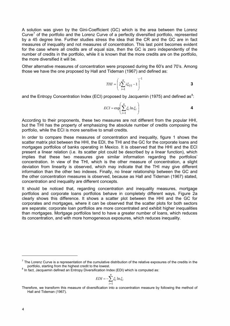
In order to compare these measures of concentration and inequality, figure 1 shows the scatter matrix plot between the HHI, the EDI, the THI and the GC for the corporate loans and mortgages portfolios of banks operating in Mexico. It is observed that the HHI and the ECI present a linear relation (i.e. its scatter plot could be described by a linear function), which implies that these two measures give similar information regarding the portfolios’ concentration. In view of the THI, which is the other measure of concentration, a slight deviation from linearity is observed, which may indicate that the THI may give different information than the other two indexes. Finally, no linear relationship between the GC and the other concentration measures is observed, because as Hall and Tideman (1967) stated, concentration and inequality are different concepts.

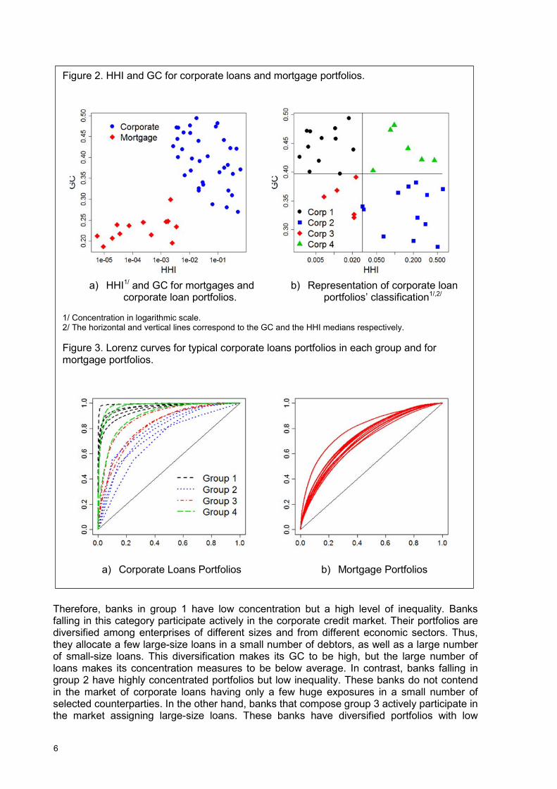
It should be noticed that, regarding concentration and inequality measures, mortgage portfolios and corporate loans portfolios behave in completely different ways. Figure 2a clearly shows this difference. It shows a scatter plot between the HHI and the GC for corporates and mortgages, where it can be observed that the scatter plots for both sectors are separate; corporate loan portfolios are more concentrated and exhibit higher inequalities than mortgages. Mortgage portfolios tend to have a greater number of loans, which reduces its concentration, and with more homogeneous exposures, which reduces inequality.

7 The Lorenz Curve is a representation of the cumulative distribution of the relative exposures of the credits in the

portfolio, starting from the highest credit to the lowest. 8 In fact, Jacquemin defined an Entropy Diversification Index (EDI) which is computed as:

∑=

−=n

iiiEDI

1lnξξ

Therefore, we transform this measure of diversification into a concentration measure by following the method of Hall and Tideman (1967).


On the other hand, corporate loans tend to have more heterogeneous exposures due to the different sectors and sizes of the enterprises and may differ significantly between banks, depending on the sectors and the size of the enterprises to which they allocate credits. The differences between banks when allocating credits impact directly their measures of concentration and inequality. In fact, banks’ portfolios may be classified into 4 groups depending on whether they are more or less concentrated, and whether they have high or low inequality. This is shown in figure 2b which plots the HHI against the GC for corporate loan portfolios. In this figure, the vertical-black line represents the median of the HHI, so that portfolios at the left side of the line are less concentrated, while portfolios at the right side are more concentrated. Similarly, the horizontal-black line represents the median of the GC: portfolios below the line have a lower measure of inequality, while portfolios over this line have higher levels of inequality.

Figure 1. Comparison between concentration measures – Herfindahl-Hirschman Index (HHI), Entropy Concentration Index (ECI), Tideman-Hall Index (THI) – and inequality measures – Gini Coefficient (GC).

* Concentration and inequality measures calculated for all Banks in the Mexican Financial System.

6

Therefore, banks in group 1 have low concentration but a high level of inequality. Banks falling in this category participate actively in the corporate credit market. Their portfolios are diversified among enterprises of different sizes and from different economic sectors. Thus, they allocate a few large-size loans in a small number of debtors, as well as a large number of small-size loans. This diversification makes its GC to be high, but the large number of loans makes its concentration measures to be below average. In contrast, banks falling in group 2 have highly concentrated portfolios but low inequality. These banks do not contend in the market of corporate loans having only a few huge exposures in a small number of selected counterparties. In the other hand, banks that compose group 3 actively participate in the market assigning large-size loans. These banks have diversified portfolios with low

Figure 2. HHI and GC for corporate loans and mortgage portfolios.

a) HHI1/ and GC for mortgages and

corporate loan portfolios. b) Representation of corporate loan

portfolios’ classification1/,2/ 1/ Concentration in logarithmic scale. 2/ The horizontal and vertical lines correspond to the GC and the HHI medians respectively. Figure 3. Lorenz curves for typical corporate loans portfolios in each group and for mortgage portfolios.

a) Corporate Loans Portfolios b) Mortgage Portfolios


inequality levels as well. As to group 4, banks in this category do not participate in this market. They assign few small-size loans, with the corresponding high concentration and inequality measures.

To go deeper in this analysis, figure 3 shows the Lorenz Curves for some representative banks of each group. It is observed that banks in group 1, which have the least concentrated portfolios, also have the highest inequality; in contrast, banks in group 4 which are the most concentrated, locate their Lorenz curves the closest to the 45 degree line, implying a lower inequality. This result may be counter intuitive, but is explained by the fact that more concentrated portfolios tend to have fewer numbers of loans.

2. Estimating Concentration under aggregate data

In order to compute any of the measures presented in last section, the complete credit portfolio is required. This may be an important limitation because in most cases, only aggregate data is available; the detail of the portfolio is unknown. This was the case for banking supervisors in Mexico in the past decade, when they only had access to detailed information on credits allocated by banks operating around the country, that were greater than a certain threshold, while credits below the threshold were aggregated and only the total exposure of the bucket was reported.

During the 80’s, many studies on industry concentration and market competition were confronted with similar problems: researchers only had access to listings of the largest firms in a given industry so that calculation of the HHI (or other measures) was not possible.

One of the first attempts to overcome this situation was due to Cowell and Mehta (1982) who proposed a “rule of thumb” derived by interpolating the histogram of the industry’s participants. Their main idea was to estimate upper and lower bounds of the tail of the Lorenz Curve from the Concentration Ratio at different levels, and then, to take a linear combination of these bounds to estimate the Gini-Coefficient of the industry. Hoffmann (1984) and Michelini and Pickford (1985) extended this approach to estimate concentration measures, especially the HHI. Mathematically, assume that the portfolio is divided in m buckets. Denote by Fk the total amount of bucket k relative to the total value of the portfolio, and by Hk the HHI in each bucket. Then, the HHI in equation 1 can be written as:

∑=

=m

kkk HFHHI

1

2

5

Now, we can compute two bounds for the HHI of the portfolio in terms of the bounds of the HHI of each bucket9. The lower bound for the HHI is, then:

∑=

=m

kk

kF

nHHI

1

2_

1

6

where nk is the number of credits in each bucket; and the upper bound is:

∑=

+ =m

kkFHHI

1

2

7

Then, the HHI of the portfolio should be a convex combination of the lower and upper bounds:

9 We know that, for a bucket composed of n credits, the HHI of the bucket is bounded between 1/n and 1.

8

( ) +− −+= HHIHHIHHI γγ 1 8

for γ∈[0, 1]. The problem now becomes to estimate the real weight γ which is an unknown parameter10. Cowell and Mehta (1982) proposed as a “rule of thumb”, to establish γ=1/3. Hoffman (1984) and Michelini and Pickford (1985) showed that this rule of thumb worked pretty well on their studies of industry concentration.

Some recent studies suggest probabilistic approaches to estimate concentration. These methods are more accurate than the rule of thumb proposed by Cowell and Mehta. Two of these methodologies are presented: one proposed by McCloughan and Abounoori (2003), and another one proposed by Kanagala et al. (2005).

The methodology proposed by McCloughan and Abounoori (2003) assumes that the portfolio is divided in size-buckets11 and that the number of credits on each bucket and its total size is provided. This information provides some points on the Lorenz Curve of the portfolio. The authors proposed to interpolate a distribution over these points, and then, to distribute the credits uniformly among the range of its bucket. The method would provide estimates of the size of each credit on the portfolio and then, it would be possible to estimate concentration12.

As for the methodology of Kanagala et al. (2005), the authors suggest to assume that the relative exposure of each credit on a given bucket (equation 5) follows a Gaussian random variable. Then, the HHI in the bucket would be a Chi-Square random variable. The main disadvantage of these methods is that it requires information on the number of credits and the standard deviation of the relative exposures in the bucket13; this information is rarely available.

Two more methodologies to estimate the HHI were suggested by Márquez (2006). The first approach assumes that the only available information on a bucket is the size of the largest credit in the bucket. Then, an upper bound for the HHI in equation 5 is:

∑=

≤m

kkk FHHI

1

2*ξ

9

where ξk* is the maximum exposure in bucket k relative to the bucket total exposure. It should

be noted that this upper bound is more accurate than the upper bound defined by equation 7. If information on the number of credits in each bucket is also available, the estimator on equation 8 could be improved using this upper bound proposed by Márquez.

The second estimator suggested by Márquez (2006), as the one proposed by Kanagala et al., is founded on the knowledge of the number of credits in a bucket and the standard deviation of the relative exposures, σX. Márquez derived an exact expression for computing the variance of the relative exposures in terms of the HHI:

∑ ∑= =

−

−=

+−

−=

−

−=

n

i

n

i

iiiX n

HHInnnnnn 1 1

22

22 1

1112

111

11 ξ

ξξσ

and then:

10 As Michelini and Pickford (1985) stated, to estimate γ we must know the real HHI, but in this case, computing

the linear combination is redundant. 11 The original method of McCloughan and Abounoori estimates the CR for different levels of k. This is why the

methodology requires the portfolio to be divided in size buckets. The approach we describe here is slightly different as our interest is in estimating concentration measures, especially the HHI.

12 Appendix A better describes this approach. 13 The average relative exposure is not required as it is the inverse of the number of credits.


( )n

nHHI X11 2 +−= σ

10

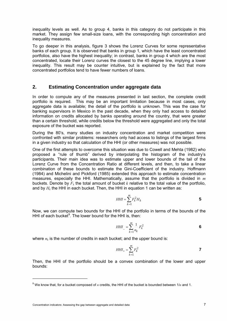
This equation shows that there is a linear relation between the portfolio HHI and the variance of the exposures in the portfolio. Thus, unbiased estimators for the HHI may be computed from unbiased estimators of the variance of the exposures and the approach of Márquez is better than that of Kanagala et al. However, the second approach may be useful for making predictions on the future concentration of the portfolio, but this is not the purpose of this paper.

Table 1 summarizes these methodologies and the information required to estimate the HHI. To assess the accuracy of these methodologies to estimate concentration when aggregate data is provided, it is assumed, as in the case of the information reported to Mexican supervisors, that loans below a given threshold are not reported in detail, but only some information is provided. Different thresholds will be considered to show how, the more information is provided, the more reliable are the concentration estimators.

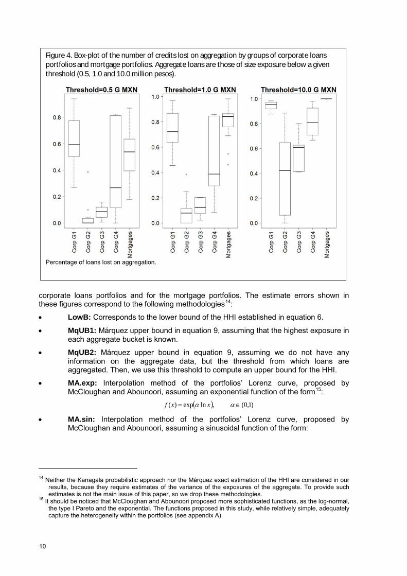
Figure 4 illustrates the number of loans that are lost on aggregation for each group of loans’ portfolios considered in last section. The thresholds that are considered are 0.5, 1.0 and 10 million pesos. It is observed that the higher the threshold is the more information is lost. The portfolios for which more information is lost are corporates in group 1 and mortgages.

The results on the estimates of the HHI are presented in figures 5, 6 and 7, for the thresholds 0.5, 1.0 and 10 million pesos, respectively. These figures show box-plots for the relative errors on the estimation of the HHI using different methodologies, for each group of

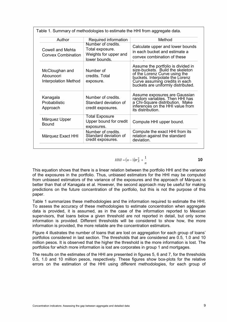
Table 1. Summary of methodologies to estimate the HHI from aggregate data.

Author Required information Method

Cowell and Mehta Convex Combination

Number of credits. Total exposure. Weights for upper and lower bounds.

Calculate upper and lower bounds in each bucket and estimate a convex combination of these b d

McCloughan and Abounoori Interpolation Method

Number of credits. Total exposure.

Assume the portfolio is divided in size-buckets. Build the skeleton of the Lorenz Curve using the buckets. Interpolate the Lorenz Curve assuming credits in each buckets are uniformly distributed.

Kanagala Probabilistic Approach

Number of credits. Standard deviation of credit exposures.

Assume exposures are Gaussian random variables. Then HHI has a Chi-Square distribution. Make inferences on the HHI value from its distribution.

Márquez Upper Bound

Total Exposure Upper bound for credit exposures.

Compute HHI upper bound.

Márquez Exact HHI Number of credits. Standard deviation of credit exposures.

Compute the exact HHI from its relation against the standard deviation.

10

corporate loans portfolios and for the mortgage portfolios. The estimate errors shown in these figures correspond to the following methodologies14:

• LowB: Corresponds to the lower bound of the HHI established in equation 6.

• MqUB1: Márquez upper bound in equation 9, assuming that the highest exposure in each aggregate bucket is known.

• MqUB2: Márquez upper bound in equation 9, assuming we do not have any information on the aggregate data, but the threshold from which loans are aggregated. Then, we use this threshold to compute an upper bound for the HHI.

• MA.exp: Interpolation method of the portfolios’ Lorenz curve, proposed by McCloughan and Abounoori, assuming an exponential function of the form15:

( ) )1,0( ,lnexp)( ∈= αα xxf • MA.sin: Interpolation method of the portfolios’ Lorenz curve, proposed by

McCloughan and Abounoori, assuming a sinusoidal function of the form:

14 Neither the Kanagala probabilistic approach nor the Márquez exact estimation of the HHI are considered in our

results, because they require estimates of the variance of the exposures of the aggregate. To provide such estimates is not the main issue of this paper, so we drop these methodologies.

15 It should be noticed that McCloughan and Abounoori proposed more sophisticated functions, as the log-normal, the type I Pareto and the exponential. The functions proposed in this study, while relatively simple, adequately capture the heterogeneity within the portfolios (see appendix A).

Figure 4. Box-plot of the number of credits lost on aggregation by groups of corporate loans portfolios and mortgage portfolios. Aggregate loans are those of size exposure below a given threshold (0.5, 1.0 and 10.0 million pesos).

Percentage of loans lost on aggregation.


)1,0( ,2

sin)( ∈

= απ αxxf

• CM.RT: “Rule of thumb” proposed by Cowell and Mehta, which is a linear combination of the HHI lower and upper bounds, equation 8 with γ=1/3.

• CM.MRT: Modified “Rule of thumb” proposed by Cowell and Mehta, changing the upper bound of the HHI to the upper bound proposed by Márquez (MqUB2), and fixing γ=1/3.

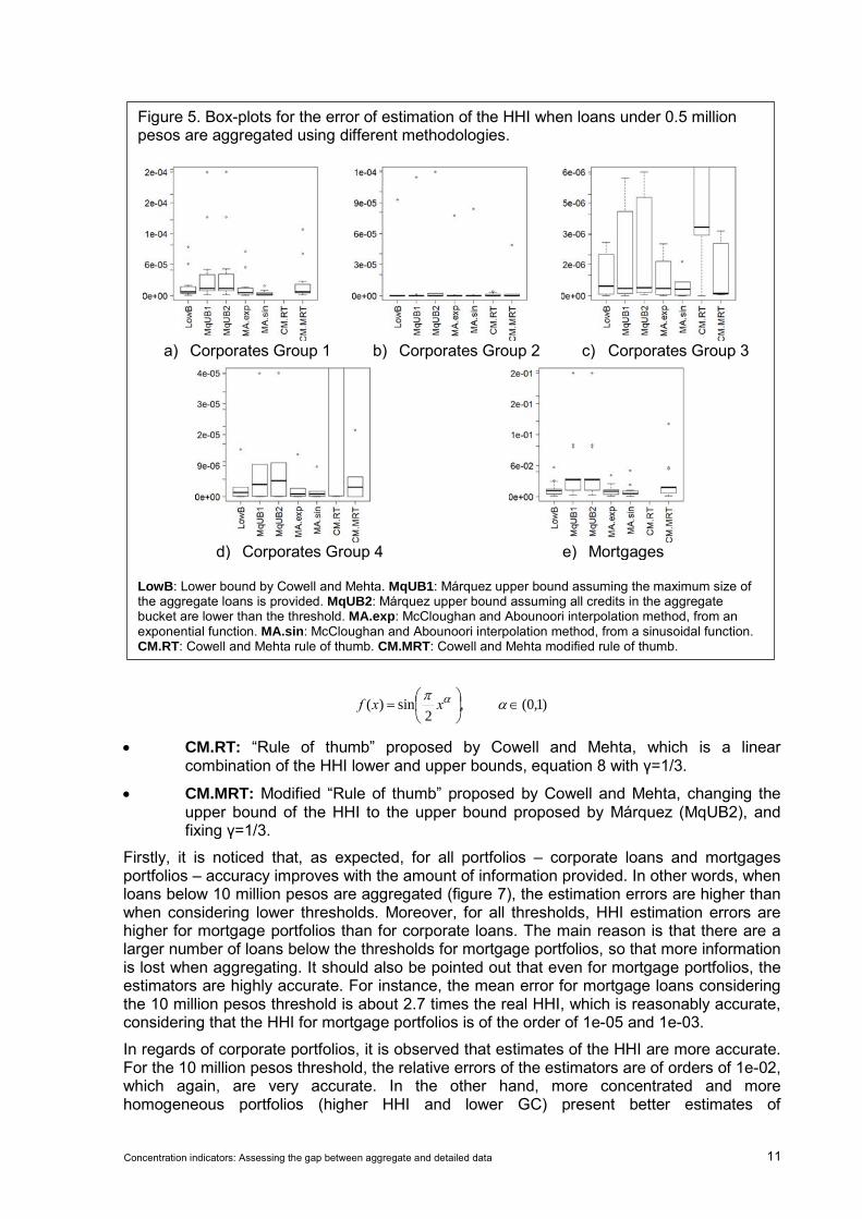
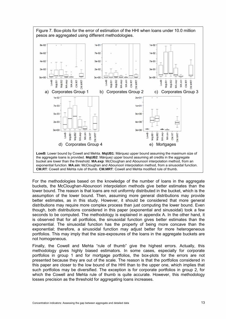
Firstly, it is noticed that, as expected, for all portfolios – corporate loans and mortgages portfolios – accuracy improves with the amount of information provided. In other words, when loans below 10 million pesos are aggregated (figure 7), the estimation errors are higher than when considering lower thresholds. Moreover, for all thresholds, HHI estimation errors are higher for mortgage portfolios than for corporate loans. The main reason is that there are a larger number of loans below the thresholds for mortgage portfolios, so that more information is lost when aggregating. It should also be pointed out that even for mortgage portfolios, the estimators are highly accurate. For instance, the mean error for mortgage loans considering the 10 million pesos threshold is about 2.7 times the real HHI, which is reasonably accurate, considering that the HHI for mortgage portfolios is of the order of 1e-05 and 1e-03.

In regards of corporate portfolios, it is observed that estimates of the HHI are more accurate. For the 10 million pesos threshold, the relative errors of the estimators are of orders of 1e-02, which again, are very accurate. In the other hand, more concentrated and more homogeneous portfolios (higher HHI and lower GC) present better estimates of

Figure 5. Box-plots for the error of estimation of the HHI when loans under 0.5 million pesos are aggregated using different methodologies.

a) Corporates Group 1 b) Corporates Group 2 c) Corporates Group 3

d) Corporates Group 4 e) Mortgages

LowB: Lower bound by Cowell and Mehta. MqUB1: Márquez upper bound assuming the maximum size of the aggregate loans is provided. MqUB2: Márquez upper bound assuming all credits in the aggregate bucket are lower than the threshold. MA.exp: McCloughan and Abounoori interpolation method, from an exponential function. MA.sin: McCloughan and Abounoori interpolation method, from a sinusoidal function. CM.RT: Cowell and Mehta rule of thumb. CM.MRT: Cowell and Mehta modified rule of thumb.

12

concentration. Indeed, group 2 portfolios, which are highly concentrated and homogeneous, have the lowest estimation errors (except for an outlier bank). As already mentioned, the reason is that these banks allocate large size credits in a few selected counterparts.

For group 1 of corporate loan portfolios, which comprises the most active banks in this sector, it is observed that the average estimation error is of the order of 1e-05 for the 0.5 million pesos threshold and 1e-02 for the 10 million pesos threshold.

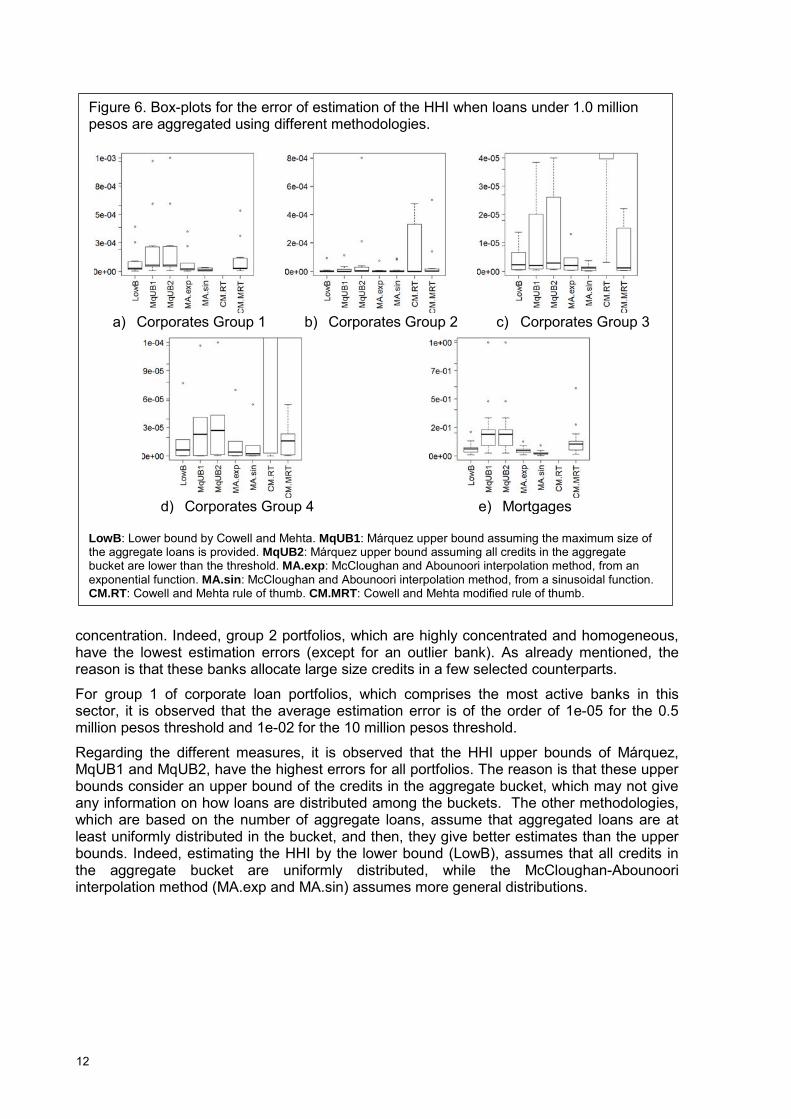
Regarding the different measures, it is observed that the HHI upper bounds of Márquez, MqUB1 and MqUB2, have the highest errors for all portfolios. The reason is that these upper bounds consider an upper bound of the credits in the aggregate bucket, which may not give any information on how loans are distributed among the buckets. The other methodologies, which are based on the number of aggregate loans, assume that aggregated loans are at least uniformly distributed in the bucket, and then, they give better estimates than the upper bounds. Indeed, estimating the HHI by the lower bound (LowB), assumes that all credits in the aggregate bucket are uniformly distributed, while the McCloughan-Abounoori interpolation method (MA.exp and MA.sin) assumes more general distributions.






For the methodologies based on the knowledge of the number of loans in the aggregate buckets, the McCloughan-Abounoori interpolation methods give better estimates than the lower bound. The reason is that loans are not uniformly distributed in the bucket, which is the assumption of the lower bound. Then, assuming more general distributions may provide better estimates, as in this study. However, it should be considered that more general distributions may require more complex process than just computing the lower bound. Even though, both distributions considered in this paper (exponential and sinusoidal) took a few seconds to be computed. The methodology is explained in appendix A. In the other hand, it is observed that for all portfolios, the sinusoidal function gives better estimates than the exponential. The sinusoidal function has the property of being more concave than the exponential; therefore, a sinusoidal function may adjust better for more heterogeneous portfolios. This may imply that the size-exposures of the loans in the aggregate buckets are not homogeneous.

Finally, the Cowell and Mehta “rule of thumb” give the highest errors. Actually, this methodology gives highly biased estimators. In some cases, especially for corporate portfolios in group 1 and for mortgage portfolios, the box-plots for the errors are not presented because they are out of the scale. The reason is that the portfolios considered in this paper are closer to the low bound of the HHI than to the upper one, which implies that such portfolios may be diversified. The exception is for corporate portfolios in group 2, for which the Cowell and Mehta rule of thumb is quite accurate. However, this methodology losses precision as the threshold for aggregating loans increases.





14

Even though, the Cowell and Mehta “rule of thumb” can be modified to create more accurate estimates of the HHI. This “modified rule of thumb” (CM.MRT), rather than considering as upper bound the one given in equation 7, it considers the upper bound proposed by Márquez (MqUB2). Then, the estimator proposed by this “modified rule of thumb” is given by:

232

31 MqUBLowBHHI +=

This modified rule of thumb gives better estimates than the simple rule of thumb of Cowell and Mehta, because the upper bound of Márquez is much closer to the real HHI than the upper bound used by Cowell and Mehta. Furthermore, more accurate estimates can be proposed by changing the weight γ. Actually, the real value of γ lies between 0.6 and 0.8 for most cases, and hence, proposing γ=2/3 may increase considerably the accuracy of the estimates of the HHI. However, computing the best value of γ may not be possible a priori, and the error of this “rule of thumb” may not be controlled.

3. Conclusions

As concentration is presumably one of the most important causes of large losses in the banks’ portfolios, banking supervisors and authorities are encouraged to monitor and evaluate the concentration risks of their financial institutions. To this end, they should have their own models to assess the capital adequacy of the banks, and furthermore, such models should be sensitive to concentration measures.

If concentration is explicitly incorporated in those models, supervisors and authorities may not need the full set of exposures of the banks’ portfolios. Instead, accurate estimates on the portfolios’ concentration may be sufficient to properly assess the capital adequacy of banks.

The paper presented some methodologies that properly fulfill this task. By comparing estimates on the HHI – one of the most popular measures of concentration – from aggregate data, against the actual index, for the credit portfolios of the Mexican banking institutions, we were able to properly assess the accuracy of some methodologies that have been proposed in the literature. Depending on the structure of the portfolios and the available information on the aggregate data, the mean relative error of the estimates lies between 1e-07 and 1e-02, which is quite accurate. Therefore, even if banking supervisors and authorities are provided with aggregate data on the credit exposures of a bank, they are able to compute estimates of concentration measures, and thus monitor the risk of banks’ portfolios and to assess their capital adequacy.

However, we should remark that concentration is not the only source of large losses in a credit portfolio, there are sources of risk that supervisors and authorities should consider, for example common exposure to the same risk factors in a single portfolio, have a direct influence on the concentration of risk, which is really the issue. In other words, even If concentration in terms of number and size of credits can be accurately estimated from aggregate data, other risk factors such as how defaults are correlated within a portfolio, may require supervisors to have access the full set of exposures of banks and its characteristics. Even though, the proper measurement of concentration is one step forward on the assessment of banks’ capital adequacy.


A. The McCloughan-Abounoori interpolation method o estimate concentration under aggregate data

This appendix is concerned on the mathematical description of the McCloughan and Abounoori (2003) interpolation method, its implementation for the cases presented in this paper, and some comments on its accuracy.

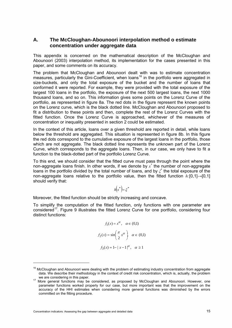
The problem that McCloughan and Abounoori dealt with was to estimate concentration measures, particularly the Gini-Coefficient, when loans16 in the portfolio were aggregated in size-buckets, and only the total exposure of the bucket and the number of loans that conformed it were reported. For example, they were provided with the total exposure of the largest 100 loans in the portfolio, the exposure of the next 500 largest loans, the next 1000 thousand loans, and so on. This information gives some points on the Lorenz Curve of the portfolio, as represented in figure 8a. The red dots in the figure represent the known points on the Lorenz curve, which is the black dotted line. McCloughan and Abounoori proposed to fit a distribution to these points and then, complete the rest of the Lorenz Curves with the fitted function. Once the Lorenz Curve is approached, whichever of the measures of concentration or inequality presented in section 2 could be estimated.

In the context of this article, loans over a given threshold are reported in detail, while loans below the threshold are aggregated. This situation is represented in figure 8b. In this figure the red dots correspond to the cumulative exposure of the largest loans in the portfolio, those which are not aggregate. The black dotted line represents the unknown part of the Lorenz Curve, which corresponds to the aggregate loans. Then, in our case, we only have to fit a function to the black-dotted part of the portfolio Lorenz Curve.

To this end, we should consider that the fitted curve must pass through the point where the non-aggregate loans finish. In other words, if we denote by x* the number of non-aggregate loans in the portfolio divided by the total number of loans, and by ξ* the total exposure of the non-aggregate loans relative to the portfolio value, then the fitted function h:[0,1]→[0,1] should verify that:

( ) ** ξ=xh

Moreover, the fitted function should be strictly increasing and concave.

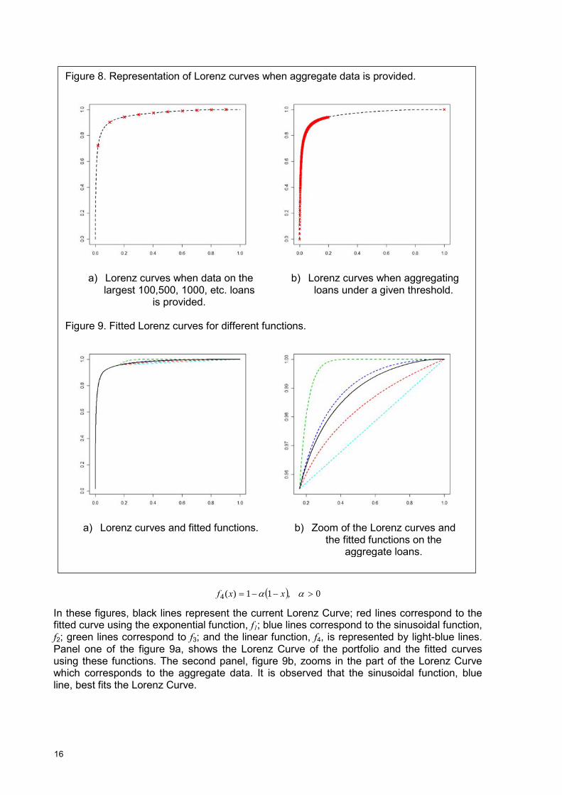
To simplify the computation of the fitted function, only functions with one parameter are considered17. Figure 9 illustrates the fitted Lorenz Curve for one portfolio, considering four distinct functions:

)1,0(,)(1 ∈= ααxxf

)1,0(,2

sin)(2 ∈

= απ αxxf

1,|1|1)(3 ≥−−= ααxxf

16 McCloughan and Abounoori were dealing with the problem of estimating industry concentration from aggregate

data. We describe their methodology in the context of credit risk concentration, which is, actually, the problem we are considering in this paper.

17 More general functions may be considered, as proposed by McCloughan and Abounoori. However, one parameter functions worked properly for our case, but more important was that the improvement on the accuracy of the HHI estimates when considering more general functions was diminished by the errors committed on the fitting procedure.

16

( ) 0,11)(4 >−−= αα xxf

In these figures, black lines represent the current Lorenz Curve; red lines correspond to the fitted curve using the exponential function, f1; blue lines correspond to the sinusoidal function, f2; green lines correspond to f3; and the linear function, f4, is represented by light-blue lines. Panel one of the figure 9a, shows the Lorenz Curve of the portfolio and the fitted curves using these functions. The second panel, figure 9b, zooms in the part of the Lorenz Curve which corresponds to the aggregate data. It is observed that the sinusoidal function, blue line, best fits the Lorenz Curve.

Figure 8. Representation of Lorenz curves when aggregate data is provided.

a) Lorenz curves when data on the

largest 100,500, 1000, etc. loans is provided.

b) Lorenz curves when aggregating loans under a given threshold.

Figure 9. Fitted Lorenz curves for different functions.

a) Lorenz curves and fitted functions. b) Zoom of the Lorenz curves and

the fitted functions on the aggregate loans.


We remark that the McCloughan-Abounoori interpolation method using the linear function, light blue line, corresponds to the HHI lower bound, where loans in the aggregate bucket are assumed to be equally distributed.

References

Bailey, D., and Boyle, S. (1971). “The Optimal Measure of Concentration”. Journal of the American Statistical Association, Vol. 66, pp.702-706.

Bajo, O., and Salas, R. (1999). “Inequality foundations of concentration measures: An application to the Hannah-Kay Indices”. Working paper.

Basel Committee on Banking Supervision (2006). “International Convergence of Capital Measurement and Capital Standards”. Bank for International Settlements.

Basel Committee on Banking Supervision (2006b). “Studies on Credit Risk Concentration: An overview of the issues and synopsis of the results from the Research Task Force project”. Bank for International Settlements, Working Paper.

Bonollo, M., Mosconi, P., and Mercurio, F. (2009). “Basel II Second Pillar: an Analytical VaR with Contagion and Sectorial Risks”. Available at SSRN: http://ssrn.com/abstract=1334953 or http://dx.doi.org/10.2139/ssrn.1334953

Clarke, R., and Davis, S. W. (1983). “Aggregate concentration, Market concentration and diversification”. The Economic Journal, Vol. 93, pp. 182-192.

Cowell, F., and Mehta, F. (1982). “The Estimation and Interpolation of Inequality Measures”. The Review of Economic Studies, Vol. 49, pp. 273-290.

Deutsche Bundesbank (2006). “Concentration risk in credit portfolios”. Deutsche Bundesbank Monthly Report: June.

Ebert, S., and Lütkebohmert, E. (2010). “Treatment of Double Default Effects within the Granularity Adjustment for Basel II”. Discussion paper.

Gordy, M. (2002). “A Risk-Factor Model Foundation for Rating-Based Bank Capital Rules”. Board of Governors of the Federal Reserve System Working Paper.

Gürtler, M., Hibbeln, M., and Vöhringer, C. (2009). “Measuring Concentration Risk for Regulatory Purposes”. Available at SSRN: http://ssrn.com/abstract=1101323 or http://dx.doi.org/10.2139/ssrn.1101323

Hall, M., and Tideman, N., (1967). “Measures of concentration”. Journal of the American Statistical Association, Vol. 62, pp. 162-168.

Hoffmann, R. (1984). “Estimation of Inequality and Concentration measures from grouped observations”. Brazilian Review of Econometrics, Vol. 04, pp. 7-21.

Jacquemin, A. (1975). “Une mesure entropique de la diversification des Enterprise”. Revue Économique, Vol. 66, pp. 834-838.

Jacquemin, A. and Berry, C. (1979). “Entropy measure of diversification and corporate growth”. The Journal of Industrial Economics, Vol. 27, pp. 359-369.

Kanagala, A., Sahni, M., Sharma, S., Gou, B., and Yu, J. (2004). “A Probabilistic Approach of Hirschman-Herfindahn Index (HHI) to Determine Possibility of Market Power Acquisition”. Power Systems Conference and Exposition, IEEE PES, Vol. 3, pp. 1277-1282.

Lütkebohmert, E. (2009). “Concentration Risk in Credit Portfolios”. EEA Lecture Note, Springer.

18

Márquez, J. (2005). “A simplified credit risk model for supervisory purposes in emerging markets”. Bank for International Settlements. Research paper.

Márquez, J. (2006). “Una nueva visión del riesgo de crédito”. Ed. Limusa, 2nd Edition.

McCloughan, P., and Abounoori, E. (2003). “How to estimate market concentration given grouped data”. Applied Economics, Vol. 35, pp. 973-983.

Michelini, C., and Pickford, M. (1985). “Estimating the Herfindahl Index from concentration ratio data”. Journal of the American Statistical Association, Vol. 80, pp. 301-305.

Vasicek, O. (1987). “Probability of Loss on Loan Portfolio”. KMV Corporation.

concentration indicators: assessing the gap between ... · concentration indicators: assessing the...

Documents