computing geodesic paths on manifolds r. kimmel j.a. sethian department of mathematics lawrence...

CComputing omputing GGeodesic eodesic PPaths on aths on MManifoldsanifolds

R. KimmelR. KimmelJ.A. SethianJ.A. Sethian

Department of MathematicsDepartment of MathematicsLawrence Berkeley Laboratory Lawrence Berkeley Laboratory

University of California, BerkeleyUniversity of California, BerkeleyProc. National. Academy of Sciences 1997Proc. National. Academy of Sciences 1997

AbstractAbstract The The Fast Marching MethodFast Marching Method is a numerical algorithm for is a numerical algorithm for

solving the solving the Eikonal equationEikonal equation on a on a rectangular rectangular orthogonal meshorthogonal mesh in in OO((MMloglogMM)) steps. steps.

MM : total number of grid points : total number of grid points We extend the We extend the Fast Marching MethodFast Marching Method to to triangular triangular

domainsdomains with the same with the same computational complexitycomputational complexity.. We provide an We provide an optimal time algorithmoptimal time algorithm for for computing computing

geodesic distancegeodesic distance and thereby extracting and thereby extracting shortest shortest pathspaths on on triangulated manifoldstriangulated manifolds..

1. Abstract2. Introduction3. The FM Method on Orthogonal Grid4. FM on a Particular Triangulated Planar Domain5. Construction of Minimal Geodesics

IntroductionIntroduction First, we review the First, we review the Fast Marching MethodFast Marching Method for for

orthogonal gridsorthogonal grids.. Then, for motivational reasons, we analyze Then, for motivational reasons, we analyze the the

structurestructure of this method of this method onon a triangulated planar grida triangulated planar grid constructed directlyconstructed directly from from an an orthogonal gridorthogonal grid..

We then We then follow withfollow with a general procedure for computing a general procedure for computing the solution of the Eikonal equationthe solution of the Eikonal equation on on arbitrary acute arbitrary acute triangulated domainstriangulated domains, followed by an extension to , followed by an extension to general (non-acute) triangulatesgeneral (non-acute) triangulates..

As an application, we compute As an application, we compute geodesic distancegeodesic distance and and minimal geodesic pathsminimal geodesic paths on on manifoldsmanifolds..

1. Abstract2. Introduction3. The FM Method on Orthogonal Grid4. FM on a Particular Triangulated Planar Domain5. Construction of Minimal Geodesics

The Fast Marching The Fast Marching Method on Orthogonal Method on Orthogonal

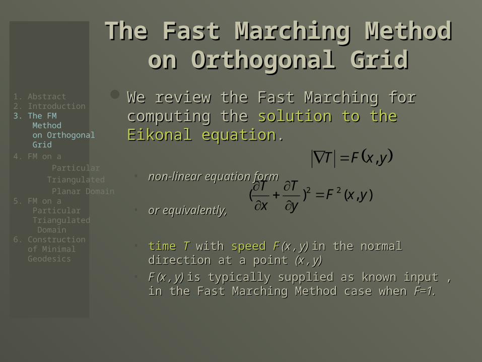
GridGrid We review the Fast Marching for computing We review the Fast Marching for computing

the the solution to the Eikonal equationsolution to the Eikonal equation..

• non-linear equation formnon-linear equation form

• or equivalently,or equivalently,

• time time TT with with speed speed FF ( (xx , y) , y) in the normal direction at a in the normal direction at a point point ((xx , y) , y)

• F (F (xx , y) , y) is typically supplied as known input , in the Fast is typically supplied as known input , in the Fast Marching Method case whenMarching Method case when F=1.F=1.

1. Abstract2. Introduction3. The FM Method on Orthogonal Grid4. FM on a • Particular • Triangulated • Planar Domain5. FM on a Particular Triangulated Domain6. Construction of Minimal Geodesics

),()( 22 yxFy

T

x

T

yxFT ,


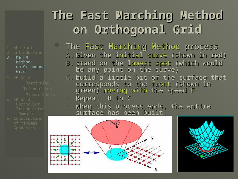
GridGrid The The Fast Marching MethodFast Marching Method process process

A.A. Given the Given the initial curveinitial curve (shown in red) (shown in red)B.B. stand on the stand on the lowest spotlowest spot (which would be any point (which would be any point

on the curve)on the curve)C.C. build a little bit of the surface that corresponds to build a little bit of the surface that corresponds to

the the frontfront (shown in green) (shown in green) moving withmoving with the speed the speed FF• Repeat B to CRepeat B to C• When this process ends, the entire surface has When this process ends, the entire surface has

been built. been built.



GridGrid The key idea is to build an a The key idea is to build an a approximation approximation to to

thethe gradient term gradient term which correctly which correctly dealsdeals with with the development of the development of corners and cuspscorners and cusps in the in the solution.solution.

The Fast Marching Method considers the The Fast Marching Method considers the nature of nature of upwindupwind , ,entropy-satisfyingentropy-satisfying approximations to the Eikonal equation (non-approximations to the Eikonal equation (non-differentiable)differentiable)..



GridGrid Entropy-satisfyingEntropy-satisfying approximations to the Eikonal approximations to the Eikonal

equation equation • Closed initial curveClosed initial curve T (T (00) ) inin

• LetLet T (t) T (t) be the one parameter family of curves, where be the one parameter family of curves, where tt is is time time

• generated by generated by movingmoving in the in the initial initial curve curve alongalong its normal its normal vector field ( vector field ( front front ))with with speedspeed FF

• Let be the Let be the position vectorposition vector which, at time which, at time t , t , parameterizesparameterizes T (t) T (t) by by ss ,,0 s S ,≦ ≦0 s S ,≦ ≦

• Travel along the curve in the direction of Travel along the curve in the direction of increasingincreasing s s

• Written in Written in term of the coordinatesterm of the coordinates• The The equationsequations of of motionmotion

,0t

tsx ,

2R

tSt xx ,,0

),(),(),,(, tsTtsytsxtsx

SssssysxTttsyttsx

SssysxTtyx

xyt

yx

yx

ss

s

ss

s

ss

st

ss

st

0;))(),(())0,(),0,((0,)(

),()(

),(

0;))0,(),0,((0,)()(

21222122

21222122



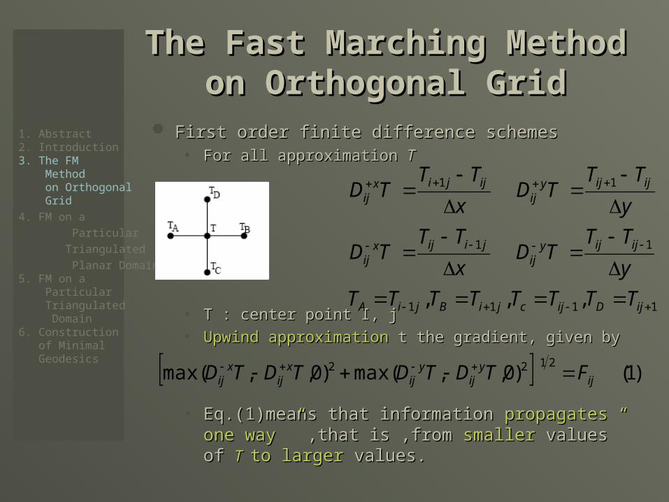
GridGrid First order finite difference schemesFirst order finite difference schemes

• For all approximation For all approximation T T

• T : center point I, j T : center point I, j

• Upwind approximationUpwind approximation t the gradient, given by t the gradient, given by

• Eq.(1)means that information Eq.(1)means that information propagates “ one propagates “ one way ”way ” ,that is ,from ,that is ,from smallersmaller values of values of T T to largerto larger values.values.

1. Abstract2. Introduction3. The FM Method on Orthogonal Grid4. FM on a • Particular • Triangulated • Planar Domain5. FM on a Particular Triangulated Domain6. Construction of Minimal Geodesics )1()0,,max()0,,max(

2122ij

yij

yij

xij

xij FTDTDTDTD

1111

11

11

,,,

ijDijcjiBjiA

ijijyij

jiijxij

ijijyij

ijjixij

TTTTTTTT

y

TTTD

x

TTTD

y

TTTD

x

TTTD


GridGrid The algorithm rests on ” solving ” Eq.(1) by building the The algorithm rests on ” solving ” Eq.(1) by building the

solution solution outward outward from the from the smallest smallest TT value. value. The algorithm is made fast by confining the “The algorithm is made fast by confining the “building building

zonezone” to a ” to a narrow bandnarrow band around the around the frontfront.. The The Fast Marching Method algorithmFast Marching Method algorithm is as follow : is as follow :

• tag points in the tag points in the initialinitial conditions as conditions as AliveAlive• tag astag as CloseClose all points all points one grid pointone grid point away away

• Tag as Tag as FarFar all all other grid pointsother grid points



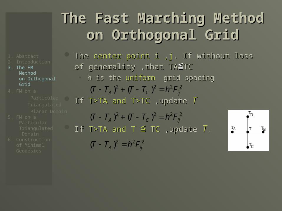
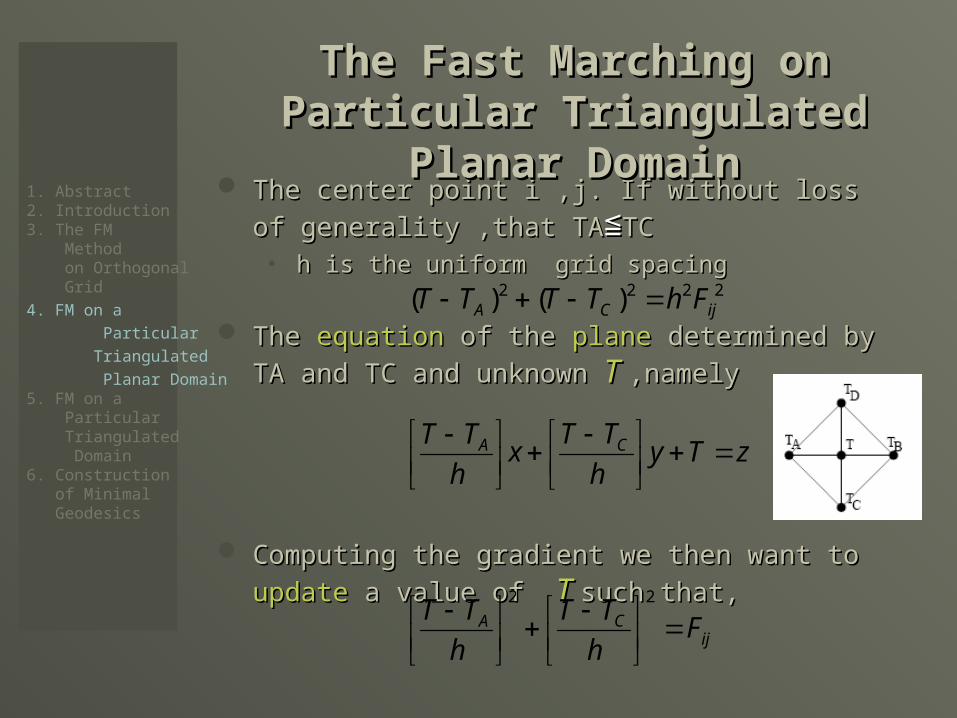
GridGrid The The center point i ,jcenter point i ,j. If without loss of generality . If without loss of generality

,that TA,that TA≦≦TC TC • h is the h is the uniformuniform grid spacing grid spacing

If If T>TA and T>TCT>TA and T>TC ,update ,update TT

If If T>TA and T T>TA and T ≦≦ TC TC ,update ,update TT..

222

2222

2222

)(

)()(

)()(

ijA

ijCA

ijCA

FhTT

FhTTTT

FhTTTT



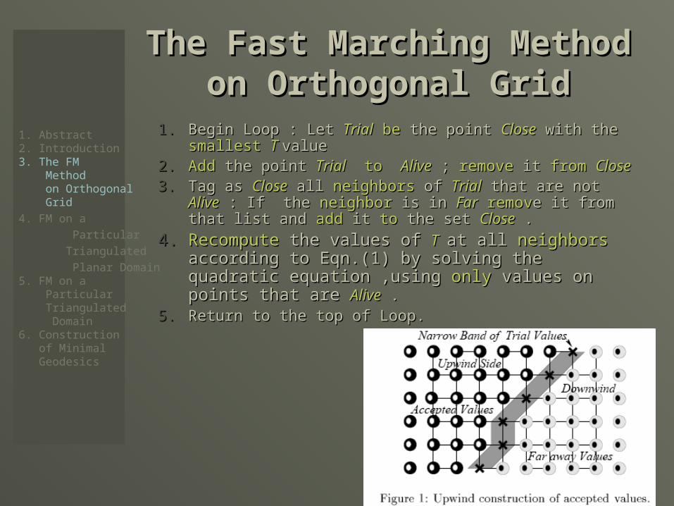
GridGrid1.1. Begin Loop : Let Begin Loop : Let TrialTrial be be the point the point CloseClose with the with the smallest smallest TT

valuevalue2.2. AddAdd the point the point TrialTrial to to AliveAlive ; ; removeremove it it from from CloseClose 3.3. Tag as Tag as CloseClose all all neighbors neighbors ofof TrialTrial that are not that are not AliveAlive : If the : If the

neighborneighbor is in is in FarFar removremove it from that list and e it from that list and addadd it it toto the the set set CloseClose . .

4.4. RecomputeRecompute the values of the values of TT at all at all neighborsneighbors according to Eqn.(1) by solving the quadratic according to Eqn.(1) by solving the quadratic equation ,using equation ,using onlyonly values on points that are values on points that are AliveAlive . .

5.5. Return to the top of Loop.Return to the top of Loop.



GridGrid This algorithm works because the process of This algorithm works because the process of

recomputingrecomputing the the TT values at values at upwind upwind neighboringneighboring points points can’tcan’t yields a value yields a value smaller thansmaller than any of the any of the AliveAlive points. points.

M total pointsM total points• The speed of the algorithm comes from a The speed of the algorithm comes from a heapsortheapsort

techniquetechnique to efficiently locate the to efficiently locate the smallest elementsmallest element in in the set the set TrialTrial. The complexity : . The complexity : OO((MMloglogMM))

• Dijkstra’s methodDijkstra’s method complexity : complexity : OO((MMloglogMM) ) , but two , but two points on the graph produces the points on the graph produces the network network minimum lengthminimum length , which may , which may notnot be optimal. be optimal.


The center point i ,j. If without loss of generality The center point i ,j. If without loss of generality ,that TA,that TA≦≦TC TC • h is the uniform grid spacingh is the uniform grid spacing

The The equationequation of the of the planeplane determined by TA determined by TA and TC and unknown and TC and unknown T T ,namely,namely

Computing the gradient we then want to Computing the gradient we then want to updateupdate a a

value of value of T T such that,such that,

ijCA

CA

ijCA

Fh

TT

h

TT

zTyh

TTx

h

TT

FhTTTT

22

2222 )()(


The Fast Marching on The Fast Marching on Particular Triangulated Particular Triangulated

Planar DomainPlanar Domain

A Construction for Acute A Construction for Acute TriangulatedTriangulated

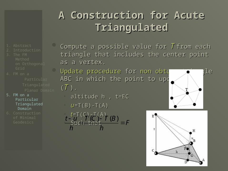
Compute a possible value for Compute a possible value for T T from each triangle that from each triangle that includes the center point as a vertex.includes the center point as a vertex.

Update procedure Update procedure forfor non obtuse non obtuse triangle ABC in triangle ABC in

which the point to update is C (which the point to update is C (T T ).).• altitude h , t=ECaltitude h , t=EC

• uu=T(B)-T(A)=T(B)-T(A)

• tt=T(C)-T(A)=T(C)-T(A)

• Such thatSuch that

1. Abstract2. Introduction3. The FM Method on Orthogonal Grid4. FM on a • Particular • Triangulated • Planar Domain5. FM on a Particular Triangulated Domain6. Construction of Minimal Geodesics F

h

BTCT

h

ut

)()(


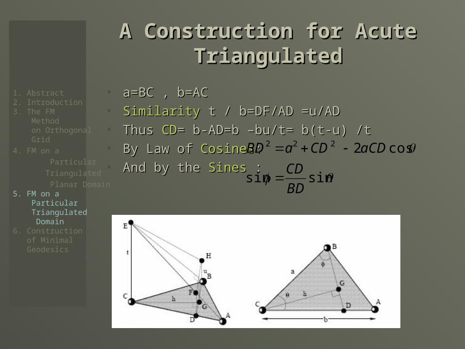
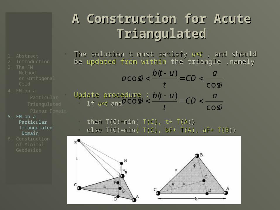
• a=BC , b=ACa=BC , b=AC• SimilaritySimilarity t / b=DF/AD =u/AD t / b=DF/AD =u/AD• Thus Thus CDCD= b-AD=b –bu/t= b(t-u) /t= b-AD=b –bu/t= b(t-u) /t• By Law of By Law of CosinesCosines: : • And by the And by the SinesSines : :

sinsin

cos2222

BD

CD

aCDCDaBD



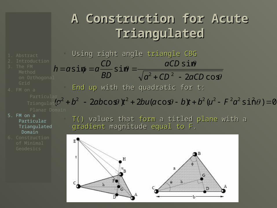
• Using right angle Using right angle triangle CBGtriangle CBG

• End upEnd up with the quadratic for t: with the quadratic for t:

• T()T() values that values that formform a titled a titled planeplane with a with a gradientgradient magnitude magnitude equal to Fequal to F..

0)sin()cos(2)cos2(

cos2

sinsinsin

22222222

22

aFubtbabutabba

aCDCDa

aCD

BD

CDaah



• The solution t must satisfy The solution t must satisfy u<tu<t , and should be , and should be updated from withinupdated from within the triangle ,namely the triangle ,namely

• Update procedure :Update procedure :• If If u<tu<t and and

• then T(C)=min{ then T(C)=min{ T(C), t+ T(AT(C), t+ T(A)})}• else T(C)=minelse T(C)=min{ T(C), bF+ T(A), aF+ T(B{ T(C), bF+ T(A), aF+ T(B)})}

cos

)(cos

cos

)(cos

aCD

t

utba

aCD

t

utba


Extension to General Extension to General TriangulationsTriangulations

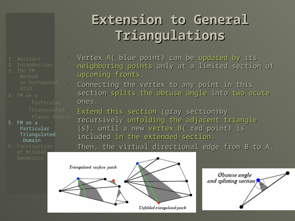
• Vertex Vertex AA( blue point) can be ( blue point) can be updated byupdated by its its neighboring pointsneighboring points only at a limited section of only at a limited section of upcoming frontsupcoming fronts..

• Connecting the vertex to any point in this section Connecting the vertex to any point in this section splits the obtuse anglesplits the obtuse angle into into two acutetwo acute ones. ones.

• Extend this sectionExtend this section (gray section)by recursively (gray section)by recursively unfolding the adjacent triangleunfolding the adjacent triangle (s), until a new (s), until a new vertex Bvertex B( red point) is included ( red point) is included in the extended in the extended sectionsection..

• Then, the virtual directional edge from B to A. Then, the virtual directional edge from B to A.



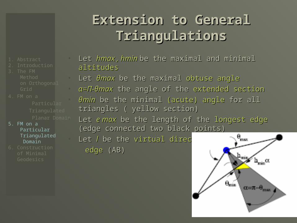
• Let Let hmax , hmin hmax , hmin be the maximal and minimal be the maximal and minimal altitudesaltitudes• Let Let θmaxθmax be the maximal be the maximal obtuse angleobtuse angle

• α=Π-θmaxα=Π-θmax the angle of the the angle of the extended sectionextended section• θminθmin be the minimal be the minimal (acute) angle(acute) angle for all triangles for all triangles

( yellow section)( yellow section)• Let Let e maxe max be the length of the be the length of the longest edgelongest edge (edge (edge

connected two black points) connected two black points) • Let Let ll be the be the virtual directionalvirtual directional

edgeedge (AB) (AB)



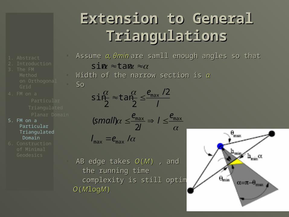
• Assume Assume α, θmin α, θmin are samll enough angles so thatare samll enough angles so that

• Width of the narrow section is Width of the narrow section is αα• SoSo

• AB edge takes AB edge takes OO((MM)) , and , and the running time the running time complexity is still optimal complexity is still optimal OO((MMloglogMM))

/2

)(

2/

2tan

2sin

tansin

maxmax

maxmax

max

el

el

l

esmall

l

e


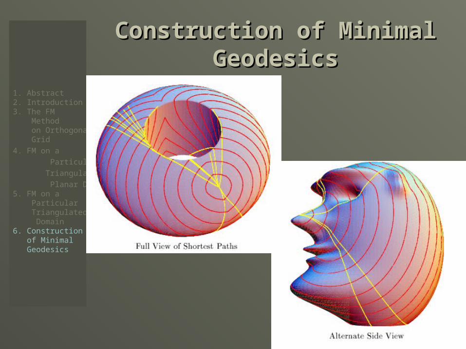
Construction of Minimal Construction of Minimal GeodesicsGeodesics

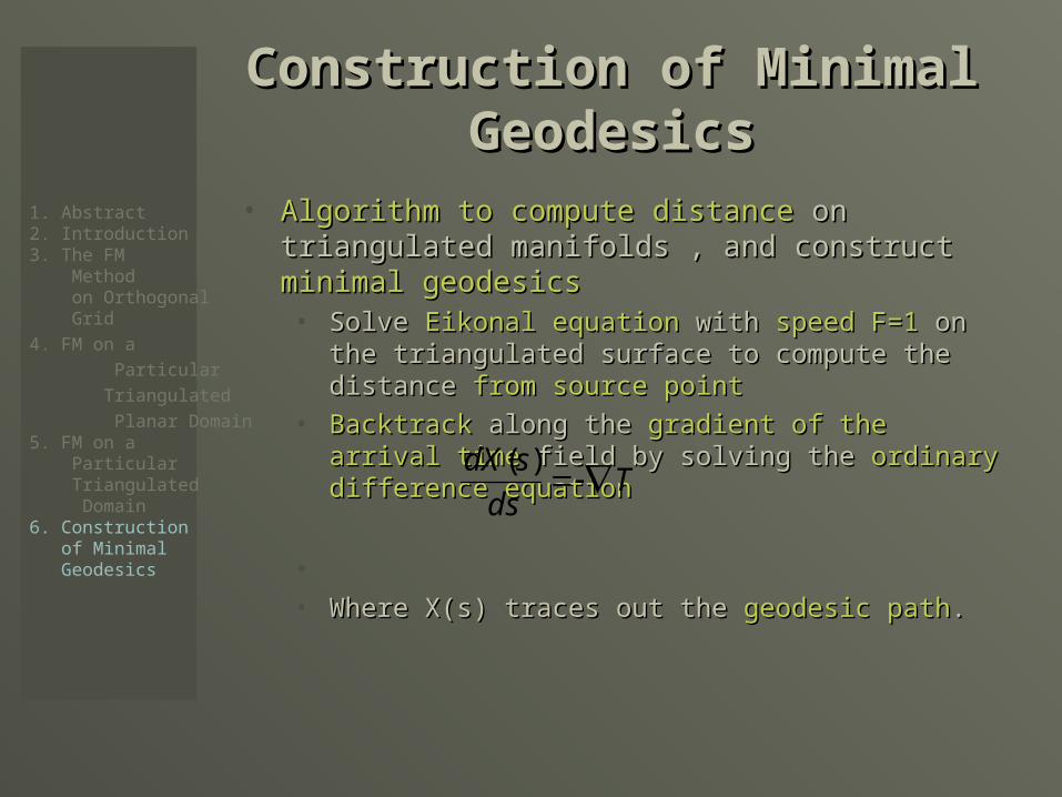
• Algorithm to compute distanceAlgorithm to compute distance on triangulated on triangulated manifolds , and construct manifolds , and construct minimal geodesicsminimal geodesics• Solve Solve Eikonal equationEikonal equation with with speed F=1speed F=1 on the on the

triangulated surface to compute the distance triangulated surface to compute the distance from from source pointsource point

• BacktrackBacktrack along the along the gradient of the arrival timegradient of the arrival time field by solving the field by solving the ordinary difference equationordinary difference equation

•

• Where X(s) traces out the Where X(s) traces out the geodesic pathgeodesic path. .

Tds

sdX

)(


Construction of Minimal Construction of Minimal GeodesicsGeodesics


computing geodesic paths on manifolds r. kimmel j.a. sethian department of mathematics lawrence...

Documents